1
Integration and Validation of Flow Image
Quantification (Flow-IQ) System
Jason Bradley Carneal
A thesis submitted to the Faculty of the Virginia Polytechnic
Institute and State University in partial fulfillment of the
requirements for the degree of
Master of Science
in
Engineering Mechanics
September 2004
Approved by ___________________________________________________
Dr. Pavlos Vlachos, Chairperson of Supervisory Committee
__________________________________________________
Dr. Demetri Telionis
__________________________________________________
Dr. Marty Johnson
Keywords: DPIV, Wall Shear, Spray, Particle Sizing, Elliptical Gaussian Profile
Copyright 2004, Jason B. Carneal
ABSTRACT
Integration and Validation of Flow Image
Quantification (Flow-IQ) System
Jason B. Carneal
The first aim of this work was to integrate, validate, and document, a digital particle image quantification
(Flow-IQ) software package developed in conjunction with and supported by Aeroprobe Corporation. The
system is tailored towards experimental fluid mechanics applications. The second aim of this work was to
test the performance of DPIV algorithms in wall shear flows, and to test the performance of several particle
sizing algorithms for use in spray sizing and average diameter calculation. Several particle sizing algorithms
which assume a circular particle profile were tested with DPIV data on spray atomization, including three
point Guassian, four point Gaussian, and least squares algorithms. A novel elliptical diameter estimation
scheme was developed which does not limit the measurement to circular patterns. The elliptic estimator
developed in this work is able to estimate the diameter of a particle with an elliptic shape, and assumes that
the particle is axisymmetric about the x or y axis. Two elliptical schemes, the true and averaged elliptical
estimators, were developed and compared to the traditional three point Gaussian diameter estimator using
theoretical models.
If elliptical particles are theoretically used, the elliptical sizing schemes perform
drastically better than the traditional scheme, which is limited to diameter measurements in the x-direction.
The error of the traditional method in determining the volume of an elliptical particle increases dramatically
with the eccentricity. Monte Carlo Simulations were also used to characterize the error associated with wall
shear measurements using DPIV. Couette flow artificial images were generated with various shear rates at
the wall. DPIV analysis was performed on these images using PIV algorithms developed by other
researchers, including the traditional multigrid method, a dynamically-adaptive DPIV scheme, and a control
set with no discrete window offset. The error at the wall was calculated for each data set. The dynamically
adaptive scheme was found to estimate the velocity near the wall with less error than the no discrete
window offset and traditional multigrid algorithms. The shear rate was found to be the main factor in the
error in the velocity measurement. In wall shear velocity measurement, the mean (bias) error was an order
of magnitude greater than the RMS (random) error. A least squares scheme was used to correct for this bias
error with favorable results. The major contribution of this effort stems from providing a novel elliptical
particle sizing scheme for use in DPIV, and quantifies the error associated with wall shear measurements
using several DPIV algorithms. A test bed and comprehensive user’s manual for Flow-IQ v2.2 was also
developed in this work.
ii
ACKNOWLEDGMENTS
The author is truly at a loss when it comes to thanks in relation to this work. The reason for this
loss is the difficulty of imagining anyone who would want to be associated with a pile of paper that
will never make any real or imaginary difference in the world as we know it. However, the one
saving grace of the acknowledgements section is that of all the theses I have picked up, the
acknowledgements are the only section I have bothered to read. So, therefore, for people like me
reading this now, I must submit:
My deepest thanks to my parents for raising me with a healthy disrespect for all those in authority.
I also owe them the need for people to earn their respect from me, rather than simply respecting
them for their shiny titles, medals, and pieces of paper. Thank you again, mom and dad, for
teaching me to be my own person, and to hell with anyone who would have me any other way.
Thank you to my precious wife, Catherine, whose example of unending kindness inspires me every
day to be more understanding and accepting of the world around me. You truly are my anchor.
Thank you to my brother, for his inspiring zest for life, and the affirmation that family and friends
must always take a front burner on the stove of life.
Thank you my friends, both at home and at school, for making this appalling waste of time, if
anything, more enjoyable and memorable. To Yaz, Ali, Jose, and Jagibbs for many hours of
support, venting time, and comradery. To Schwartz, for keeping the dream alive.
And finally, to anyone who is reading this thesis now, for putting it down before continuing on
and wasting any more of your precious time on this earth.
Dream out loud.
iii
Everything you know is wrong.
-interference from zoo tv
iv
TABLE OF CONTENTS
CHAPTER 1 ..................................................................................................................................1
1
BACKGROUND AND INTRODUCTION.......................................................................1
1.1
1.2
1.2.1
1.2.2
1.2.3
1.2.4
1.3
1.4
MOTIVATION ...................................................................................................................1
PARTICLE IMAGE VELOCIMETRY ....................................................................................1
METHOD ..........................................................................................................................1
IMAGE PROCESSING AND MAXIMUM RESOLVABLE DISPLACEMENT ..............................6
TRADITIONAL MULTIGRID TECHNIQUE ..........................................................................7
DISCRETE WINDOW OFFSET ...........................................................................................7
PARTICLE TRACKING VELOCIMETRY ............................................................................10
ERROR ANALYSIS ..........................................................................................................10
CHAPTER 2 ................................................................................................................................12
2
PIV SIZING OF SPRAY DATA, ANALYSIS AND COMPARISON TO PDA........12
2.1
2.1.1
2.1.1.1
2.1.1.2
2.1.1.3
2.1.1.4
2.1.1.5
2.2
2.2.1
2.2.2
2.2.3
2.2.4
2.2.5
2.3
2.3.1
2.3.2
2.4
2.4.1
2.4.2
2.4.3
2.4.4
2.5
2.6
INTRODUCTION ..............................................................................................................12
CONVENTIONAL PARTICLE SIZING TECHNIQUES ..........................................................14
AXIS-SYMMETRIC GAUSSIAN SHAPE ........................................................................14
THREE POINT GAUSSIAN FIT .....................................................................................15
FOUR POINT GAUSSIAN ESTIMATOR .........................................................................16
CONTINUOUS FOUR POINT FIT ..................................................................................17
CONTINUOUS LEAST SQUARES GAUSSIAN FIT .........................................................18
EXPERIMENTAL METHODS AND MATERIALS ................................................................18
SPRAY GENERATION .....................................................................................................18
DPIV SYSTEM ...............................................................................................................18
DPIV SOFTWARE ..........................................................................................................20
PDA SYSTEM ................................................................................................................20
COMPUTATIONAL AND COMPUTER RESOURCES ...........................................................24
SPRAY DPIV/PDA COMPARISON .................................................................................24
HISTOGRAM ANALYSIS .................................................................................................25
AVERAGE DIAMETER ANALYSIS ...................................................................................26
PARTICLE SIZING RESULTS ...........................................................................................26
FULL-RANGE RESULTS .................................................................................................26
LIMITED-RANGE RESULTS ............................................................................................27
AVERAGE DIAMETER ....................................................................................................35
PTV-CORRECTED HISTOGRAMS ...................................................................................40
CONCLUSIONS AND FUTURE WORK ..............................................................................44
SUMMARY OF ORIGINAL CONTRIBUTION......................................................................45
CHAPTER 3 ................................................................................................................................47
3
ELLIPTICAL PARTICLE SIZING METHOD ............................................................47
v
3.1
3.2
3.3
3.3.1
3.3.2
3.4
3.4.1
3.4.2
3.5
INTRODUCTION ..............................................................................................................47
ELLIPTICAL PARTICLE SIZING SCHEME METHODS AND MATERIALS ...........................51
ELLIPTICAL PARTICLE SIZING RESULTS ........................................................................51
THEORETICAL FOUNDATIONS .......................................................................................52
EXPERIMENTAL ANALYSIS ............................................................................................56
CONCLUSIONS AND FUTURE WORK. .............................................................................65
LOG NORMAL / NORMAL INDEPENDENT (LNNI) PDF. ................................................66
RAYLEIGH NORMAL INDEPENDENT (RNI) PDF. ..........................................................67
SUMMARY OF ORIGINAL CONTRIBUTION......................................................................70
CHAPTER 4 ................................................................................................................................71
4
WALL SHEAR EXPERIMENTS ....................................................................................71
4.1
4.2
4.3
4.3.1
4.3.1.1
4.3.1.2
4.3.2
4.4
4.5
INTRODUCTION ..............................................................................................................71
WALL SHEAR METHODS AND MATERIALS ...................................................................72
WALL SHEAR RESULTS .................................................................................................73
LOW SHEAR RATE STUDY .............................................................................................73
COMPARISON TO UNIFORM DISPLACEMENT MEASUREMENTS .................................77
TRACKING RESULTS ..................................................................................................78
HIGH SHEAR RATE STUDY ............................................................................................79
CONCLUSIONS AND FUTURE WORK ..............................................................................90
SUMMARY OF ORIGINAL CONTRIBUTION......................................................................90
CHAPTER 5 ................................................................................................................................92
5
DPIV DOCUMENTATION AND TEST BED ...............................................................92
5.1
5.2
5.2.1
5.2.1.1
5.2.1.2
5.3
DPIV VERSION 1.0 DOCUMENTATION ..........................................................................92
TEST BED FOR DPIV SOFTWARE, METHODS ..............................................................177
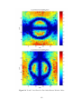
TEST BED FOR FLOW-IQ V2.2 RESULTS......................................................................177
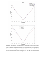
UNIFORM DISPLACEMENT RESULTS. ......................................................................178
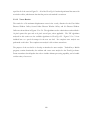
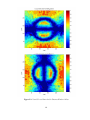
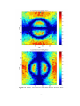
VORTEX RESULTS. ..................................................................................................180
SUMMARY OF ORIGINAL CONTRIBUTION....................................................................184
REFERENCES..........................................................................................................................185
VITA ...........................................................................................................................................188
vi
LIST OF FIGURES
FIGURE 1.1: ILLUSTRATION OF INTERROGATION WINDOWS AND OVERLAP ...................................3
FIGURE 1.2: CROSS-CORRELATION PROCEDURE ............................................................................4
FIGURE 1.3: GENERIC EXPERIMENTAL SETUP ................................................................................5
FIGURE 1.4: BLOCK DIAGRAM FOR THE ESTIMATION OF VELOCITY VECTORS ..............................6
FIGURE 1.5: TRADITIONAL MULTIGRID METHOD..........................................................................7
FIGURE 1.6: FIRST ORDER DISCRETE WINDOW OFFSET ................................................................8
FIGURE 1.7: SECOND ORDER DISCRETE WINDOW OFFSET PIV ....................................................9
FIGURE 2.1: ESM FLUID MECHANICS LABORATORY DPIV SYSTEM..........................................20
FIGURE 2.2: EXPERIMENTAL SETUP FOR THE SPRAY PIV AND PDPA EXPERIMENT ...................23
FIGURE 2.3: EXAMPLE DIGITAL PARTICLE IMAGE VELOCIMETRY SPRAY DATA, 0MM PLANE ..25
FIGURE 2.4: FULL RESULTS FOR ALL SIZING METHODS AND PDA, 0MM PLANE .......................27
FIGURE 2.5: RESULTS FOR ALL SIZING METHODS AND PDA, 100 TO 150 MICRONS, 0MM PLANE
...............................................................................................................................................28
FIGURE 2.6: HISTOGRAM RESULTS FOR - 4MM SPRAY PLANE, ALL SIZING METHODS ...............29
FIGURE 2.7: HISTOGRAM RESULTS FOR + 4MM SPRAY PLANE, ALL SIZING METHODS ..............30
FIGURE 2.8: HISTOGRAM RESULTS FOR +/- 8MM SPRAY PLANE, ALL SIZING METHODS. ..........31
FIGURE 2.9: PLANE-AVERAGED HISTOGRAM RESULTS FOR ALL PIV SIZING METHODS ...........32
FIGURE 2.10: PLANE-AVERAGED RESULTS FOR 3 POINT GAUSSIAN METHOD AND PDA. .........33
TABLE 2.1: PARTICLE POPULATION FOR EACH METHOD, 0MM PLANE .......................................34
TABLE 2.2: PARTICLE POPULATION FOR EACH METHOD, 0MM PLANE .......................................34
FIGURE 2.11: CORRELATION COEFFICIENT VS. PLANE FOR CONVENTIONAL SIZING METHODS. 35
FIGURE 2.12: 3-D ISOSURFACE PLOT OF AVERAGE DIAMETER...................................................36
FIGURE 2.13: CORRESPONDING SLICE HEIGHT IN 3-D. ...............................................................37
FIGURE 2.14: PDA AND 3 POINT GAUSSIAN PIV AVERAGE DIAMETER, Z = 15.4MM.................39
FIGURE 2.15: TOTAL POPULATION HISTOGRAMS FOR 3 POINT GUASSIAN, TRACKING, AND PTVCOMPENSATED METHODS, SPRAY 0MM PLANE......................................................................40
FIGURE 2.16: PDA, 3 POINT GAUSSIAN, PTV, AND PTV-COMPENSATED PDF’S, 0MM PLANE ..41
TABLE 2.3: PTV CORRELATION COEFFICIENTS FOR FULL RANGE RESULTS, 0 MM PLANE ........42
FIGURE 2.17: PTV-COMPENSATED AND PDA HISTOGRAMS, 0MM PLANE ..................................42
FIGURE 2.18: POPULATION FOR PIV/PTV METHODS AND PDF’S FOR PIV, PDA, AND PTV ......43
TABLE 2.4: PTV CORRELATION COEFFICIENTS FOR 100 TO 150 UM RANGE, 0 MM PLANE ........44
FIGURE 2.19: TRACKING COMPENSATION AND PDA FOR 100 TO 150 MICRON RANGE. .............44
FIGURE 3.1: DIAGRAM OF AN ELLIPSE. .........................................................................................48
FIGURE 3.2: JOINTLY GAUSSIAN IIRV’S WITH σX = σY. .............................................................49
FIGURE 3.3: JOINTLY GAUSSIAN IIIRV’S WITH VARIOUS VALUES OF σX AND σY.......................51
FIGURE 3.4: THEORETICAL AREA CALCULATION ERROR VS. ECCENTRICITY FOR
CONVENTIONAL SIZING METHOD .........................................................................................53
FIGURE 3.5: THEORETICAL ERROR VS. AXIS RATIO FOR 3 POINT GAUSSIAN SIZING METHOD...54
FIGURE 3.6: THEORETICAL PERCENT ERROR FOR 3 POINT GAUSSIAN, AVERAGED ELLIPTIC, AND
TRUE ELLIPTIC SIZING METHODS .........................................................................................55
vii
FIGURE 3.7: THEORETICAL PERCENT ERROR FOR 3 POINT GAUSSIAN, AVERAGED ELLIPTIC, AND
TRUE ELLIPTIC SIZING METHODS .........................................................................................56
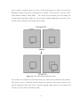
FIGURE 3.8: SAMPLE MONTE CARLO SIMULATION IMAGES........................................................57
FIGURE 3.9: ALL DATA POINTS FOR ECCENTRICITY = 0, DIAMETER RANGE 2.8 TO 5.6 PIXELS ..58
FIGURE 3.10: AVERAGED TOTAL ERROR OVER 250 POINTS, ECCENTRICITY = 0. .......................59
FIGURE 3.11: ERROR IN THE X AND Y DIAMETER MEASUREMENTS VS. X DIAMETER ...................61
FIGURE 3.12: X AND Y DIAMETER VS. ECCENTRICITY FOR EACH SIZING METHOD......................62
FIGURE 3.13: AREA ABSOLUTE AND PERCENT ERROR FOR ALL SIZING METHODS ........................64
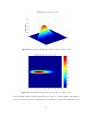
FIGURE 3.14: LOG-NORMAL SURFACE PLOT FOR σX = 0.80, σY = 0.30, µX = 1.00 , µY = 0.00 ...67
FIGURE 3.15: LOG-NORMAL CONTOUR PLOT FOR σX = 0.80, σY = 0.30, µX = 1.00 , µY = 0.00 ..67
FIGURE 3.16: LOG-NORMAL SURFACE PLOT FOR σY = 0.20, µY = 0.00, S = 6.00 ........................69
FIGURE 3.17: LOG-NORMAL CONTOUR PLOT FOR σY = 0.20, µY = 0.00, S = 6.00 .......................69
FIGURE 4.1: ARTIFICIAL IMAGE DIAGRAM FOR WALL SHEAR EXPERIMENTS ............................72
FIGURE 4.2: TOTAL ERROR FOR ALL DPIV METHODS, WINDOW 64 ...........................................74
FIGURE 4.3: TOTAL ERROR FOR ALL DPIV METHODS, WINDOW 32 ...........................................75
FIGURE 4.4: TOTAL ERROR FOR ALL DPIV METHODS, STARTING WINDOW 16..........................76
FIGURE 4.5: WALL SHEAR ERROR COMPARED TO UNIFORM DISPLACEMENT ERROR................77
TABLE 4. 1: TRACKED PARTICLE POPULATIONS FOR EACH SHEAR RATE ...................................78
FIGURE 4.6: TOTAL ERROR FOR ALL PIV METHODS AND PTV....................................................79
FIGURE 4.7: MEAN, RMS, AND TOTAL ERROR FOR NO DISCRETE WINDOW OFFSET. ...............81
FIGURE 4.8: MEAN, RMS, AND TOTAL ERROR FOR MULTIGRID DPIV ALGORITHM. ................83
FIGURE 4.9: MEAN, RMS, AND TOTAL ERROR FOR DADPIV ALGORITHM. ..............................85
FIGURE 4.10: ERROR FOR MULTIGRID, DADPIV, AND NDWO FOR VARIOUS SHEAR RATE, 64
WINDOW................................................................................................................................87
FIGURE 4.11: ERROR FOR MULTIGRID, DADPIV, AND NDWO FOR VARIOUS SHEAR RATE, 32
WINDOW................................................................................................................................89
FIGURE 5.1: MEAN, RMS, AND TOTAL ERRORS FOR ULTIMATE AND FLOW-IQ V2.2 NDWO
AND FODWO ......................................................................................................................179
FIGURE 5.2: X AND Y LOCAL ERROR FOR NO DISCRETE WINDOW OFFSET .............................181
FIGURE 5.3: X AND Y LOCAL ERROR FOR FIRST ORDER DISCRETE WINDOW OFFSET .............182
FIGURE 5.4: X AND Y LOCAL ERROR FOR FIRST ORDER DISCRETE WINDOW OFFSET .............183
viii
CHAPTER 1
1
1.1
BACKGROUND AND INTRODUCTION
Motivation
The purpose of this work is to expand the usability and accuracy of Digital Particle Image
Velocimetry (DPIV) in several significant applications. These applications include whole-field
particle diameter and mass flux calculations in sprays, the measurement of wall shear, and the
performance of novel sizing techniques on DPIV velocity measurement accuracy. The first focus
of this work is the analysis of errors associated with particle diameter and velocity measurements
using DPIV in conjunction with novel particle sizing techniques.
PIV allows a full two-
dimensional analysis of particle diameter as compared to the traditional Phase Doppler
Anemometry (PDA) measurements. This paper explores the application and performance of
novel particle sizing techniques to the measurement of particle diameter and mass flux in sprays.
The second focus of this paper is the performance of traditional and novel PIV algorithms in the
measurement of wall shear.
Wall shear, especially in boundary layer analyses, contributes
significant error to velocity measurements using DPIV. This work explores the errors involved in
the measurement of shear rate with DPIV and provides some novel methods for correcting these
errors. The third portion of this work explores the application of novel sizing techniques to
displacement estimation algorithms used in DPIV, and the errors associated with each method.
1.2
1.2.1
Particle Image Velocimetry
Method
Particle Image Velocimetry (PIV) is the process of analyzing consecutive digital images of data
using cross correlation in regions of interest to estimate a displacement in the image. This
displacement is then converted to a velocity using the frame rate of the camera, which is a known
experimental parameter.
A great deal of study has been performed on PIV and methods to
improve the accuracy of the method. Digital Particle Image Velocimetry (DPIV) has emerged as a
1
standard in global flow measurements. In this technique, a fluid is seeded with neutrally buoyant,
reflective microparticles and interrogated with a sheet of light expanded from a high-power laser
(Willert and Gharib, 1991)). Reflected light from the particles is recorded using a digital CMOS
camera with high frame rate (generally 30 Hz). Time-resolved systems (TRDPIV) such as the one
developed and employed by our group use CMOS cameras with kHz sampling rates (Abiven and
Vlachos, 2002). Images of the seeded flow are captured successively within a very short time
interval, so that the particles in a single frame appear in the previous and subsequent frames as
well. Velocity is obtained by measuring the displacement between particles in successive frames
through cross-correlation (Westerweel, 1997). The two accepted ways of resolving displacement
are DPIV and DPTV.
DPIV applications typically use digital imaging technology, since it is possible to acquire and store
a large amount of data on a computer. Digital images are characterized by their intensity pixel
values corresponding to the ones given by the camera sensors. One pixel thus defines the smallest
element of a digital image. In DPIV, images are usually coded in an 8-bit grayscale, with each pixel
taking a value between 0 and 255. An intensity value of 0 represents a black pixel, and an intensity
value of 255 represents a white pixel (Abiven and Vlachos, 2002).
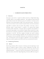
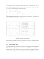
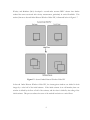
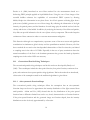
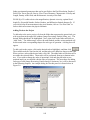
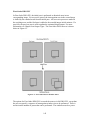
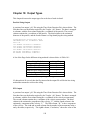
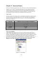
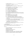
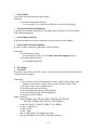
In DPIV, the target image pair is divided into subdivisions called interrogation windows. Each
subdivision is processed independently to calculate a local velocity vector. The subdivisions are
determined by the grid spacing and interrogation window size. Grid spacing is the space between
measurements in the image. For example, a grid spacing of 4 pixels means that the final output
will have a velocity every 4 pixels in the image, or a 64 X 64 grid of velocity measurements for an
image size of 256 pixels. Typically, interrogation window sizes range from 8 to 128 pixels,
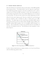
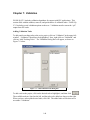
depending on the size of the digital image and the seed particle size and seeding density. Figure 1.1
below illustrates an image broken down into four interrogation windows with no overlap on the
left. This case represents no overlap between the velocity measurements. On the right, the 50%
overlap case is shown, along with the resulting measurement grid (Abiven and Vlachos, 2002).
2
Figure 1.1: Illustration of interrogation windows and overlap
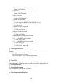
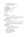
In order to get a displacement out of each interrogation window, a process called cross-correlation
is performed. Typically, fast-Fourier transforms (FFT’s) are used to calculate the cross-correlation
between two corresponding interrogation windows from successive images. However, direct
correlation and normalized methods have also been used in the past. Figure 1.2 illustrates the
DPIV process. In essence, the cross-correlation shifts the second window across the first, and
sums the matching values. At the point where the images match best, the correlation is at its peak
value. This peak is located and provides the best estimate for the displacement of the particles in
the window (Abiven and Vlachos, 2002).
There are several sources of error in DPIV that prevent the deterministic evaluation of the flow
field. Particles are moving in and out of a frame, and the particles within the same window do not
necessarily have diverse velocities. Also, particles might appear differently from one frame to the
other in terms of light intensity or shape as they move within the light sheet. The combination of
3
all these phenomena coupled with noise from the recording media constitute a random process
that introduces significant error levels to the measurement (Abiven and Vlachos, 2002).
Figure 1.2: Cross-correlation procedure
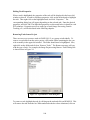
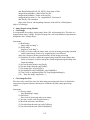
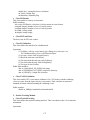
Both DPIV and DPTV use digital images as an input. A typical experimental setup for DPIV is
shown below in Figure 1.3.
4
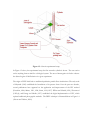
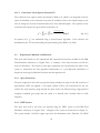
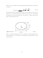
Figure 1.3: Generic experimental setup
In Figure 1.3 above, the experimental setup for flow around a cylinder is shown. The test section
can be anything from an airfoil to a biological system. The area of interrogation is fixed to observe
the desired region of fluid behavior in a given experiment.
The origin of DPIV hails back to traditional qualitative particle-flow visualizations. The early work
of Meynard (1983) established the foundations of its present form. Over the past two decades,
several publications have appeared on the application and improvement of the PIV method
(Hasselinc, 1988; Adrian, 1991, 1996; Grant, 1994, 1997). Willert and Gharib (1991), Westerweel
(1993a,b), and Huang and Gharib (1997) established the digital implementation of PIV, which
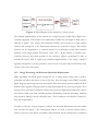
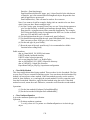
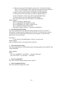
replaced traditional photographic methods. The DPIV technique is illustrated below in Figure 1.4
(Abiven and Vlachos, 2002).
5
Figure 1.4: Block Diagram for the estimation of velocity vectors
The standard implementation of the method uses a single-exposure, double-frame, digital crosscorrelation approach. CCD cameras are commercially available that can sample at frame rates of
1000 fps or higher. The velocity field calculated in DPIV can be treated as a linear transfer
function that corresponds to the displacement between two consecutive images. This transfer
function can be interpreted in a statistical manner by incorporating second-order statistical
moments of the image patterns (Westerweel, 1993a, 1997). In this manner, a statistical crosscorrelation between the particle patterns of two successive images is performed in order to
calculate the velocity field. A typical cross-correlation implementation of the velocity evaluation
algorithm will produce a velocity grid with a vector every 8 to 16 pixels with an uncertainty of the
velocity on the order of 0.1 pixels.
1.2.2
Image Processing and Maximum Resolvable Displacement
DPIV algorithms can benefit greatly through the use of image pre-processing tasks to remove
boundaries and reduce the effects of noise in the data. Since the images used in DPIV are purely
digital, image pre-processing tools were developed to allow direct phase separation within the flow.
Khalitov and Longmire (1999) presented an image-based approach for resolving two-phase flows
between a flow tracer and a solid phase. In this work, previously implemented methods by Abiven
and Vlachos (2002) were used, including dynamic thresholding, Gaussian smoothing, Laplacian
edge detection, filtering, erosion, and many more. These techniques are included in Chapter 5,
Flow-IQ documentation.
In order to satisfy the Nyquist frequency criterion, the measured displacement must be smaller
than one-half the length of the interrogation window in order to prevent aliasing effects..
However, previous work (Keane and Adrian, 1990) illustrated that the statistical cross correlation
6
velocity evaluation has the maximum confidence levels when the displacement is less than one
quarter of the interrogation window size. In this work, one quarter of the interrogation window
size is referred to as the maximum resolvable displacement.
1.2.3
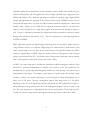
Traditional Multigrid Technique
The tradidtional iterative multigrid DPIV employs a first cross-correlation pass in order to
generate an initial predictor of the velocity-field. On the subsequent passes, the size of the
interrogation window is dynamically allocated, based on the results from the previous step
(Scarano & Rieuthmuller, 1999) as shown by figure 1.5.
Figure 1.5: Traditional Multigrid Method
Each initial window is broken down into several windows. The size of the consecutive windows
depends on the velocity obtained from the first pass.
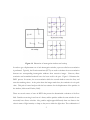
1.2.4
Discrete Window Offset
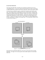
The window offset feature introduced by Westerweel (1997) represented a real breakthrough in
DPIV. This feature significantly improves the accuracy of the DPIV method. Using the first
estimate obtained from the initial DPIV pass, a second pass is applied by shifting the interrogation
window in the second image by the rounded displacement found during the first pass. The first
7
pass is subject to particles going in and out of the interrogation area, while the second pass
dramatically reduces this effect, as illustrated by the Figure 1.6. This process is known as First
Order Discrete Window Offset DPIV.
The second cross-correlation pass after shifting the
second image interrogation window by the previously estimated displacement provides a more
accurate velocity evaluation (Abiven and Vlachos, 2002).
Figure 1.6: First Order Discrete Window Offset
The second cross-correlation is preformed between two windows that contain the same particles.
The signal to noise is drastically increased during this operation. The iterative nature of this
process significantly reduces the effects of spatial averaging, which improves the resolution and
accuracy of system (Abiven and Vlachos, 2002).
8
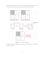
Wereley and Meinhart (2001) developed a second-order accurate DPIV scheme that further
reduced the errors associated with velocity measurement, particularly in vertical flowfields. This
method, known as Second Order Discrete Window Offset PIV, is illustrated below in Figure 1.7.
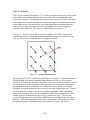
Figure 1.7: Second Order Discrete Window Offset PIV
In Second Order Discrete Window Offset PIV, the interrogation windows are shifted in both
images by a value half of the initial estimate. If the initial estimate is an odd number, then one
window is shifted by the floor of half of the estimate, and the other is shifted by the ceiling of the
initial estimate. This process reduces the error of the method in relation to vortical flows.
9
1.3
Particle Tracking Velocimetry
Digital Particle Tracking Velocimetry is defined as the tracking of particles as they progress in
DPIV data. The DPTV method used in this work utilizes the output from particle sizing and PIV
algorithms to track particles. The particles in two consecutive frames are detected, and the local
velocity from PIV is used to search for a particle within a given radius of the expected velocity. If
a particle is found, this particle is used to estimate the displacement between this particle and the
particle from the original frame . Other developed methods use size, shape, brightness, or
closeness criteria for particle differentiation and identification. The difference in particle position
serves as the displacement estimation in DPTV. The major difficulty in DPTV is the ability to
distinguish unique particles. However, DPTV eliminates the averaging effect seen in DPIV results.
The Hybrid DPTV method (Abiven and Vlachos, 2002) is used in this work.
DPTV is classified in the same general category as DPIV, since they are similar methods based on
similar fundamentals (Dracos and Gruen, 1998; Adrian et. al., 1995; Prasad and Adrian, 1993;
Adrian, 1996). In DPTV, the velocity is determined from the displacement of particles within a
fixed time interval. The major experimental difference between the methods is that the DPTV
algorithms need low seeding density, whereas PIV algorithms require relatively high seeding
density. Seeding density is the number of tracer particles in a given frame or window. DPTV is
limited to slower flows than PIV (Abiven and Vlachos, 2002).
Guezennec and Kiritsis (1990) developed the first DPTV algorithms based on DPIV, which uses
the DPIV output as a priori knowledge for the search of particles. The estimation of the
displacement is uncomplicated. A simple search radius is input by the user in order to define the
search area around the predicted velocity from DPIV results. Most particles will be detected by a
correctly-designed DPTV algorithm, given optimal experimental conditions (Abiven and Vlachos,
2002).
1.4
Error Analysis
The major error analysis technique used in this work is the Monte Carlo Simulation. In a Monte
Carlo Simulation for PIV, artificial data with a known displacement field are generated. Then, the
PIV method in question is performed on the artificial data. Errors are calculated by comparing the
10
PIV output with the known input. The major error sources are bias error and random error. Bias
error, or mean error, represents a true bias in the measurement and indicates a consistent error in
the measurement. Random error, or RMS error, quantifies the expected error in the measurement
that does not fit a specific pattern. Total error is the complete error of the measurement, and
consists of the random and bias errors summed in quadrature. The equations for total, bias, and
random error are given below in equations 1.4.1 to 1.4.3. The reliability of this error analysis
increases with the number of measurements performed in the simulation.
E total
(j)
⎡1
=⎢
⎣⎢ N
E mb (j) = D r (i,
⎡1
E rms (j) = ⎢
⎢N
⎣
∑
D r (i,
n =1
j) −
⎛
⎜ Dm (i,
∑
⎜
n =1 ⎝
N
2
N
1
N
j) − D m (i, j)
⎤
⎥
⎦⎥
1/ 2
(Eq. 1.4.1)
N
∑ D (i, j)
n =1
⎞
j) - ∑ Dm (i, j) ⎟⎟
N n =1
⎠
1
N
(Eq. 1.4.2)
m
2
⎤
⎥
⎥
⎦
1
2
(Eq. 1.4.3)
In equations 1.4.1 through 1.4.3, Dm is the measured displacement, Dr is the real (known)
displacement, N is the number of measurements performed in the simulation, Etotal is the total
error of the measurement, Emb is the bias error of the measurement, and Erms is the random error
of the measurement.
11
Chapter 2
2
PIV SIZING OF SPRAY DATA, ANALYSIS AND COMPARISON TO PDA
The purpose of this chapter was to explore the performance of the conventional sizing techniques
developed by Brady et al. (2002) in a real-world spray atomization experiment. DPIV analysis was
performed on a 60-degree conical, high-pressure spray that generated a poly-dispersed droplet
distribution. Measurements were preformed for five planes parallel to the spray axis, and separated
by 4mm. A CMOS camera recorded the DPIV images at sampling rate of 10 KHz. Advanced
image processing techniques were employed to identify the droplets and calculate their diameter
using the novel Flow-IQ software. Subsequently, the size distribution of each droplet was
quantified using geometric optics theory to convert the droplet image information to the true
droplet size. The droplet sizes from our direct imaging DPIV system were validated using a Phase
Doppler Particle Analyzer (PDPA). The calculated sizes from the direct imaging methodology
were found to agree with the measured PDPA results for droplets images larger than 3 to 4 pixels.
Resolution limitations introduced inaccuracy for smaller droplets.
This preliminary effort
illustrates the potential of performing global time resolved size measurements using a simple
DPIV configuration based on CMOS imaging technology.
2.1
Introduction
Simultaneous time resolved velocity and size measurements are limited to single point
methodologies using Phase-Doppler Particle Analyzer (PDPA). Although these methods can
measure with high accuracy the particle velocity and size they are limited by the requirement of
spherical particles (Kim et al. 1999). In the case of spay atomization this requirement is not
satisfied since the droplets deform, forming ellipsoids. In addition, single point methodologies do
not reveal the global temporal variation of the flow. The above limitations generate the need for
alternative, global measurement methodologies based on visualization techniques.
The dynamics of spray-droplet break-up, and the accurate measurement of droplet sizes and
velocities in high-pressure sprays is an increasingly important problem in fluid mechanics. During
12
the past decade there has been a wide spread use of DPIV techniques employed on the analysis of
single phase or multi-phase flow systems. DPIV measurements provide global instantaneous
velocity distributions revealing the internal structure of the flow. However, despite the numerous
advances of the method in polydispersed multi-phase flows, very few attempts have been made to
deliver simultaneous velocity, size, and shape quantification of the dispersed phase (Abiven et al.,
2002).
Simultaneous time resolved velocity and size measurements are limited to single point
methodologies using Phase-Doppler Particle Analyzer (PDPA). Although these methods can
measure with high accuracy the particle velocity and size they are limited by the requirement of
spherical particles (Kim et al. 1999). In the case of spay atomization this requirement is not
satisfied since the droplets deform, forming ellipsoids. In addition, single point methodologies do
not reveal the global temporal variation of the flow. The above limitations generate the need for
alternative, global measurement methodologies based on visualization techniques.
Khalitov and Longmire (2002) presented an image-based approach for resolving two-phase flows
between a flow tracer and a solid phase. In their approach they were able to successfully
discriminate the coexisting phases in the flow by employing image-processing principles. However,
they did not carry out any size quantification. Recent efforts combine size measurements with
DPIV using either fluorescence-Mie scattering ratio (Boedec and Simoens 2001) or interferometry
principles (Damaschke et el. 2002) to carry out the sizing tasks. Boedec and Simoens (2001) by
employing a fluorescence-Mie scattering ratio methodology were able to accurately measure the
velocity and size distribution in a high-pressure spray. However, such implementations require
complicated experimental setups, multiple cameras, optical filters and calibration for the
fluorescence intensity quantification. Damaschke et el. (2002) use Global Phase Doppler (GPD)
which is an interferometry based methodology where the particle/droplet diameter is proportional
to the number of fringes formed by out of focus particle images. Despite the high accuracy and the
global character of the method, the optical resolution of the system can be a limiting parameter
soon generating overlapping particle images because of the out of focus effects while it is limited
to small interrogation areas.
13
Pereira et al. (2000) introduced an out-of-focus method for size measurements based on a
defocusing DPIV principle applied on liquid bubble flows. Using the out of focus images of the
recorded bubbles enhances the capabilities of conventional DPIV systems by allowing
bubble/droplet size information in two-phase flows. An off-axis aperture collecting light from a
point source (bubble) generates an out-of-focus image. By collecting the information of the light
intensity, the particle pattern, and the blurriness for each image pair, the method resolves both the
velocity and the size of the bubble. In addition, by analyzing the intensity of the defocused particle,
Airy disks can provide information for the out-of-plane velocity component. This method requires
a minimum of three cameras in order to overcome measurements ambiguities.
This discussion although not comprehensive, represents some of the most recent and significant
contributions in simultaneous global velocity and size quantification methods. However, all of the
above methods do not resolve the time depended characteristics of the flow since they are limited
to sampling rates in the order of 15-30Hz. Especially in the case of spray atomization where the
natural unsteadiness of the flow is the dominant parameter that governs the break-up dynamics
sampling rates in the order of KHz are necessary.
2.1.1
Conventional Particle Sizing Techniques
The conventional particle sizing techniques used in this work were developed by Brady et al.
(2002). These techniques include the three point Gaussian, four point Gaussian, continuous four
point, and continuous least squares particle sizing algorithms. Before the methods are introduced,
a discussion of the assumptions made in the traditional algorithms is given below.
2.1.1.1
Axis-symmetric Gaussian Shape
The conventional particle sizing techniques follow the assumption that an axis-symmetric
Gaussian shape can be used to approximate the intensity distribution of the light scattered from
small particles. Adrian and Yao (1985) showed that the Airy distribution of the point spread
function from a diffraction limited lens can be very closely characterized as a Gaussian function.
If the point spread function and the geometric image are Gaussian shaped, then the intensity
distribution can also be closely approximated by a Gaussian.
14
In a PIV data set, the recorded particle image, dt can be expressed in terms of the particle diameter,
d, the diffraction limited spot diameter, ds, and the resolution of the recording medium, dr. This
relationship is shown below in Equations 2.1 to 2.3.
dt = de + d r
2
2
2
(Eq. 2.1)
ds = 2.44(M +1) f # λ
2 12
de = (M 2d 2 + d s )
(Eq. 2.2)
(Eq. 2.3)
In these equations, M is the magnification, f# is the numerical aperture of the lens, and λ is the
wavelength of a coherent monochromatic light source. Equation 1.4.3 includes the combined
effects of the optical system’s magnification and diffraction on the particle image when optical
aberrations are not present.
Gaussian fitting schemes such as the three-point estimator and local-least squares estimator reduce
the error associated with particle center estimation of a geometric image when compared to more
traditional methods such as center of mass (Udrea et al. 1996; Marxen et al. 2000, Willert and
Gharib 1991). In addition, these techniques also decrease the peak locking effect in the bias-error
when compared to centroid analysis (Willert and Gharib, 1991).
The use of the conventional Gaussian sizing schemes for finding particle positions has been
documented further in Brady et al. (2002). Other studies, such as Marxen et al. (2000), have also
investigated the use of the three point fit as a sizing algorithm. The conventional Gaussian sizing
techniques developed by Brady et al. (2002) are given in the following sections.
2.1.1.2
Three Point Gaussian Fit
The traditional three-point Gaussian estimator is a simple one-dimensional approximation of the
geometric particle image.
ai = I oe
−
( xi − xc ) 2
15
2σ 2
(Eq. 2.4)
The three independent variables Io, σ , and xc represent the maximum intensity, the Gaussian
distribution standard deviation and the center position, respectively. If the three points chosen to
solve these equations are the maximum intensity pixel, and the two neighboring pixels along the xaxis, then the standard three-point Gaussian estimator can be derived (Willert and Gharib 1991).
xc = xo +
ln ao−1 −ln ao+1
2(ln ao−1 +ln ao+1 −2 ln ao )
(Eq. 2.5)
The equation for finding the y center position is identical to equation 2.5 above. The diameter
measurement is directly related to the variance. The variance is given below in equation 2.6.
σ2 =
ln ao +1 − ln ao
( xo − xc ) 2 − ( xo +1 − xc ) 2
(Eq 2.6)
The three point estimator is computationally fast, and very easy to implement (Brady et al., 2002).
The major limitation of the diameter measurements made in Brady et al. are the use of a single
dimension as the diameter measurement and the assumption that the particles are, in fact, circular
in profile.
2.1.1.3
Four Point Gaussian Estimator
The four point Gaussian estimator was developed in order to overcome the limitations of the
three-point Gaussian fit and allow determining the center and diameter of a particle when it
contains saturated pixels. In this scheme, saturated particles do not contribute to the measurement
of diameter. The removal of saturated pixels from the calculation allows for a more accurate
estimation of the Gaussian shape of the particle, and reduces the error of the method (Brady et al.,
2002).
In order to derive the four point Gaussian estimator, Brady et al. (2002) considered the twodimensional intensity distribution given below in equation 2.7.
−
a = Ioe
( xi − xc ) 2 + ( yi − yc ) 2
i
2σ 2
(Eq. 2.7)
Four independent intensities were solved in order to arrive at the following set of equations.
These intensities were used to derive equation 1.4.8 below, which is the equation used for variance
in the four point Gaussian scheme.
16
α1 = x4 2 ( y2 − y3 ) + ( x2 2 + ( y2 − y3 )( y2 − y4 ))( y3 − y4 ) + x3 2 ( y4 − y2 )
α 2 = x4 2 ( y3 − y1 ) + x3 2 ( y1 − y4 ) − ( x12 + ( y1 − y3 )( y1 − y4 ))( y3 − y4 )
α 3 = x4 2 ( y2 − y1 ) + x2 2 ( y1 − y4 ) − ( x12 + ( y1 − y2 )( y1 − y4 ))( y2 − y4 )
α 4 = x3 2 ( y2 − y1 ) + x2 2 ( y1 − y3 ) − ( x12 + ( y1 − y2 )( y1 − y3 ))( y2 − y3 )
σ2 =
( x4 − xc ) 2 + ( y 4 − y c ) 2 − ( x3 − xc ) 2 − ( y3 − y c ) 2
2(ln( a 3 ) − ln( a 4 ))
(Eq. 2.8)
If the points selected are the same as the three point estimator, then equation 2.8 reduces to
equation 2.6. The points selected for the four-point Gaussian estimation are by no means arbitrary
and will not always yield a unique solution. Two conditions must be met for the method to
produce a solution. Firstly, a3 cannot be equal to a4, or the denominator in equation 2.8 will go to
zero. The second criterion is that the four selected points cannot all lie in a circle of any arbitrary
center or radius (Brady et al., 2002).
2.1.1.4
Continuous Four Point Fit
The three and four point fits will contain an error even without the presence of noise sources due
to the digital medium pixel discretization. In order to address this error, Brady et al. (2002)
developed a continuous four point scheme.
The continuous four point fit eliminates the
systematic error introduced by pixel descretization. The continuous four point scheme corrects
for pixel discretization through equating an integrated Gaussian profile over each pixel with the
discrete gray value (Brady et al., 2002).
ai = ∫∫ I o e
−
( xi − xc ) 2 + ( yi − yc ) 2
2σ 2
dydx
(Eq. 2.9)
Equation 2.9 cannot be solved in closed-form, and the expanded equations are shown below in
Equation 2.10 where Erf is the error function. In this equation, xi and yi represent the position of
the lower corner of each pixel (Brady et al., 2002).
ai =
(x − x )
(x + 1 − x )
(y −y )
(y + 1 − y )
π Ioσ2
c ]) (Erf[ i c ] − Erf[ i
c ])
(Erf[ i c ] − Erf[ i
2
2σ
2σ
2σ
2σ
(Eq. 2.10)
Brady et al. (2002) used a form of the Powell dogleg optimization routine to solve these nonlinear
equations. The same point selection criteria in the four point Gaussian fit apply to the continuous
four point fit.
17
2.1.1.5
Continuous Least Squares Gaussian Fit
The continuous least squares scheme, developed by Brady et al. (2002) is an integrated local least
square fit. Similarly to the continuous four point fit, introduced above, this scheme improves the
error by taking into account the discretization error of the individual pixels. The equation for the
continuous least squares fit is given below in equation 2.11
χ = ∑ (ai − ∫∫ I o e
2
−
( xi − xc ) 2 + ( yi − yc ) 2
2σ 2
dydx) 2
(Eq. 2.11)
In equation 2.11, χ2 was minimized using a Gauss-Newton algorithm. Point selection was
determined by the 3X3 area surrounding the peak intensity pixel (Brady et al, 2002).
2.2
Experimental Methods and Materials
This work relied heavily on the experimental and computational resources available in the ESM
Fluid Mechanics Laboratory at Virginia Tech. A summary of the major resources used in this
work is found below. The objective of this pilot experiment was to demonstrate the ability of the
system to characterize the time depended characteristics of a poly-dispersed distribution of
droplets by resolving the individual velocities and their apparent size.
2.2.1
Spray Generation
The spray employed in this study was generated using a 60deg cone angle nozzle and a pressure of
approximately 10Psi was applied. A low-speed, annular co-flow was introduced but was not
seeded. The water pressure going through the spray nozzle was delivered using a high-precision
computer controlled gear pump and was varied as a sinusoid with a desired offset at 10Hz
frequency.
2.2.2
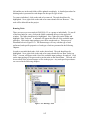
DPIV System
The spray data used in this work was acquired using the DPIV system in the ESM Fluid
Mechanics Laboratory at Virginia Tech. A diagram of the system is shown below in Figure 2.1.
The system includes a 60-Watt copper-vapor laser for illumination and a Phantom V4 CMOS
18
digital camera for data acquisition. This system allows data acquisition up to a frame rate of 1kHz.
The camera has a resolution of 512X512 pixels. The spray data used in this work was taken at a
resolution of 256X256 pixels.
A 10KHz pulsing Copper Vapor Laser was used to deliver a sheet of light with illumination energy
of 5 mJ. The laser sheet was passed through a cylindrical lens and focused into a vertical plane
parallel to the axis of the spray. A Phantom-V CMOS camera placed normal of the laser sheet
captured the water droplets with pixel resolution of 256x256 and a frame rate of 10 KHz and total
sampling time of 1 sec. A second Phantom–IV CMOS camera with resolution of 128x128 and
sampling rate of 10KHz was employed in order to record off-axis-images in a stereo DPIV
configuration. A calibration target was used to assure that the interrogation areas of the two
cameras overlap and subsequently used for the reconstruction of the images. Due to space
limitations in this paper and the preliminary nature of this study, we will not elaborate on the
three-dimensional measurements.
The laser and the camera were synchronized in order to operate in a single pulse per frame mode.
The camera is equipped with an internal shutter, which was set at 10microsecs in order to reduce
the ambient background light thus increasing the signal to noise ratio of the images. The laser
pulse and the shutter trigger to the camera were synchronized and controlled with a
PC/workstation. A multifunction National Instruments 6025E board was used to control the data
acquisition. Two 20MHz digital counters with timing resolution of 50nsecs were used to generate
the sequence of pulses necessary to accurately trigger the laser and the camera. Once the laser and
the camera received the trigger pulses, a feedback signal was recorded in order to assure the
accurate timing of the process. The overall timing uncertainly of the control system accounting
also for the laser pulse jitter was estimated in the order of 1nsec which is negligible for the velocity
ranges of approximately 10m/s measured during this experiment.
19
Figure 2.1: ESM Fluid Mechanics Laboratory DPIV system.
2.2.3
DPIV Software
The DPIV software used throughout this work consisted of in-house software. For the spray
particle sizing results with tradtitional sizing algorithms, DPIV version 1.0 was used. DPIV version
1.0 is a DPIV software package developed by Aeroprobe, Inc. This software includes DPIV
algorithms, sizing algorithms, particle tracking velocimetry, image pre-processing, and postprocessing options for DPIV in a single Windows-based platform. The user’s manual for DPIV
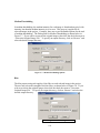
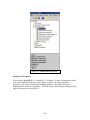
version 1.0, written by the author of this work, can be found in Appendix A.
DOS-based DPIV software was also used in this work in the wall shear studies. This software
gives the user the ability to select several processing algorithms not yet available in DPIV v1.0, and
allows processing at high speed in a DOS environment. This software is known as “Ultimate,”
and was developed by Claude Abiven and Dr. Pavlos Vlachos in the ESM Fluid Mechanics
Laboratory at Virginia Tech.
2.2.4
PDA System
To confirm the feasibility of this method and quantify the accuracy of our system, a validation
experiment comparing our system and a PDA system was performed. A one-dimensional Phase
Doppler Particle Analyzer (PDPA) was used to measure the spray droplet size and velocity in the
axial direction. It was a commercial system consisting of an integrated optical unit, a signal
20
processor, and software for system setup, data acquisition and data analysis. The integrated optical
unit encompassed a 10-mW He-Ne laser as the laser source (λ = 632.8 nm). Transmition was via
a fiber optic probe, 60-mm in diameter, which encompassed necessary optics to transmit the red
laser beams with an initial beam separation of 38mm. The focal length of the lens used for the
transmitting probe was 400-mm. The PDA receiver was another fiber optical probe, 60-mm in
diameter, with a focal length of 160-mm. It was positioned in the forward scatter mode, at a
scattering angle of 35 degrees, to allow measurements of droplet size in the reflection mode.
Given this arrangement, the fringe spacing was 6.67 µm with probe volume dimensions of
approximately 250 µm in all directions. The PDA receiver probe was configured for a maximum
particle diameter of 147 µm. A refractive index of n = 1.334 was assumed for the water spray
droplets.
Sampling at a point was performed for 60 seconds or 100,000 particle counts. The average data
rate in the core of the spray was approximately 1 kHz, this rate decreasing as the probe volume
interrogated the edges of the spray. Autocorrelations at various points in the spray (near the core)
gave an integral time scale of approximately 2.5 ms. Consequently, the statistical uncertainty of the
mean PDA data (velocity and particle size) was estimated at less than 1%.
The signal processor used FFT technology to determine the velocity and phase difference. Three
detectors were used to extend the diameter range without compromising resolution.
The
resolution of the system was 16 bits on the selected bandwidth (typically 3.75 MHz), thus yielding
negligible velocity and phase resolution uncertainty.
The location of the PDA probe volume was fixed in space while the spray was traversed relative to
it so that measurement data can be obtained over several points along a cross-plane located
approximately 15-mm from the nozzle.
A total of 189 measurement points within a plane approximately 15mm above the spray with a
total sampling time of 1min were acquired.
21
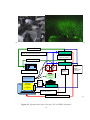
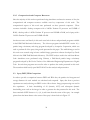
Figure 2 below shows (a) the experimental setup employed in this study including the two cameras
and the Dantec PDA system, (b) a view of the high-pressure conical spray illuminated by the laser
sheet, and (c) a schematic overview of the timing, synchronization and control arrangement.
The experiment involved the acquisition of several planes parallel to the center plane of the spray.
A total of five planes placed at -8, -4, 0, 4, and 8 mm with respect to the center plane were
acquired reconstructing a volume of the flow. The volumetric data were subsequently used to
generate the statistical distributions of the droplet sizes for horizontal planes (normal to the spray
axis). These statistics were compared with the corresponding PDA measurements
22
(a)
(b)
Transferring Images
Camera 2 (Phantom IV)
Green Lines Transferring Images to PC
Synch Signal from
Camera 1 to Camera 2
Transferring Images
Camera 1 (Phantom V)
Particle Image
Sequence
Data Processing Workstation
Synch
Signal to
Camera 2
Blue Line:
Trigger
Signal to
Camera 1 and
Camera 2
Light Sheet
Delivery
Closed Loop Positioning
Control for Laser Sheet and
Cameras Field of View
Control PC
Synchronizin
g
Laser/Camer
a
System
Synch
Signal
to
Laser
Laser 1 (ACL 45)
Black Lines: Synch Signal to
Laser and Camera
Red Lines Feedback Signal into DA Board
Figure 2.2: Experimental Setup for the Spray PIV and PDPA experiment
23
(c)
2.2.5
Computational and Computer Resources
Since the majority of this work was performed using simulations and massive amounts of data, the
computational and computer resources available were key components of this work.
computational aspects of this work were performed on three personal computers.
The
These
resources included a desktop computer with a 2.8GHz Pentium IV processor and 512MB of
RAM, a desktop with a 1.8GHz Pentium IV processor and 256MB of RAM, and a laptop with a
2.4GHz Pentium IV processor and 512MB of RAM.
Another resource used heavily in this work were both in-house and purchased programs available
in the ESM Fluid Mechanics Laboratory. The in-house programs included DPIV version 1.0, a
particle image velocimetry and sizing program developed by Aeroprobe Corporation, which was
used to perform all of the spray sizing results presented in this paper. The artificial images used in
this work were created using in-house artificial image generation software developed by Claude
Abiven in the ESM Fluid Mechanics laboratory. The DPIV analyses used in the wall shear Monte
Carlo simulations were performed using Ultimate, a DOS-based particle image velocimetry
program developed by Dr. Pavlos Vlachos of the Mechanical Engineering Department at Virginia
Tech. Several other programs were used in order to produce the results presented in this work.
The researcher relied heavily upon MATLAB 6.5 for data analysis and presentation.
2.3
Spray DPIV/PDA Comparison
In order to provide a comparison between DPIV and PDA data, the particle size histogram and
average diameter for each method was calculated and compared. Spray data from a previous
experiment was analyzed using our DPIV version 1.0b software. Image preprocessing was used in
this experiment.
A basic thresholding of 20 (intensity 0-255) and subsequent dynamic
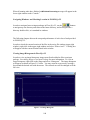
thresholding were used on the images in order to generate the data presented in this work. The
data contained a DPIV dataset at -8, -4, 0, 4, and 8 mm from the center of the spray. An example
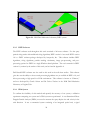
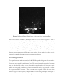
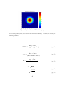
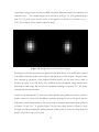
picture from the 0mm dataset at the center of the spray is shown below in Figure 2.3.
24
Figure 2.3: Example Digital Particle Image Velocimetry Spray Data, 0mm Plane
Each of these datasets included 16,304 images similar to the one shown in Figure 2.2. Each of
these frames was analyzed using each method studied in this work. The methods used in this
work were the three-point Gaussian, four-point Gaussian, continuous four-point Gaussian, and
continuous least-squares sizing methods. A total of 81,520 images were processed using each
method, combining to a total of 326,080 images processed. The experimental magnification in this
experiment was approximately 24 microns per pixel. Diffraction terms were included in all of the
diameter conversions and analysis. Bin ranges were matched for each method in order to provide
completely comparable histograms between measurement techniques.
2.3.1
Histogram Analysis
The output from each method was analyzed in MATLAB to produce histograms for each method.
Histograms were created for each plane of data. The total volume and total method histograms
were also calculated. In order to account for multiply-counted particles in the histogram, particle
tracking was run on the complete set of images, and tracked particles were removed to produce
the compensated DPIV histograms. These histograms were compared to PDA data over various
diameter ranges in order to quantify the performance of DPIV sizing techniques with respect to
25
traditional particle sizing techniques. All histograms were normalized with the total particle
population in order to produce probability density functions (pdf’s) for analysis.
2.3.2
Average diameter Analysis
In order to calculate the average diameter in the DPIV data, a volume was constructed with userdefinable resolution. The volume was constructed such that the z component moved across
planes of data with the x and y direction in the plane of the DPIV data. The output from each
method was scanned and each particle was added to a region of the volume. If the x and y
position of a particle was in a particular region, the average diameter was updated assuming the
particle to be a perfect sphere.
2.4
Particle Sizing Results
This section presents the results for the traditional sizing algorithms used in this experiment and
their histogram comparison to PDA measurements, and the average diameter analysis performed
in this work.
2.4.1
Full-Range Results
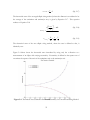
The full theoretical range of the PIV sizing methods extends to less than one pixel diameter.
However, at these low diameters, the error in the PIV measurement increases dramatically. It is,
however, important to characterize the behavior of the PIV sizing methodologies on real data at
these diameters. The magnification in this experiment was approximately 24 microns per pixel
(diffraction terms were included in the calculation of the magnification factor). Therefore, the
approximate lower limit of detectable diameter in this experiment is approximately 15 to 20
microns. The PDA system used in this experiment could resolve diameters as low as 0.5 microns.
Therefore, in this particular experimental setup, the PIV method could not resolve diameters at the
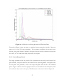
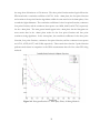
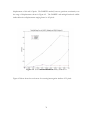
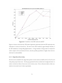
lower range of the PDA data. The full results from the 0mm plane are shown below in Figure 2.4.
26
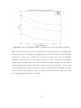
Figure 2.4: Full Results for All Sizing Methods and PDA, 0mm Plane
The results in Figure 2.4 show that there is a significant locking on particles in the 20 to 30 micron
range for all of the PIV sizing algorithms. The correlation coefficients for the three point
Gaussian, four point Gaussian, continuous four point Gaussian, and the continuous least squares
are 0.1465 , 0.2762, 0.2465, and 0.5882, respectively for this plane
2.4.2
Limited-Range Results
The sizing algorithms used in this portion of the experiment were the three point Gaussian, four
point Gaussian, four point continuous, and continuous least squares algorithms. Histogram results
for each plane were generated, as well as an average histogram results for all of the combined
planes. Figure 2.5 below shows the single plane results for each method in the 0mm plane, which
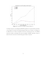
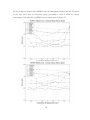
is located in the direct center of the spray. The PDA results are also shown below in Figure 2.5.
27
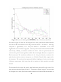
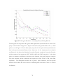
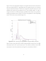
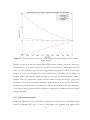
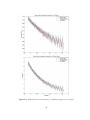
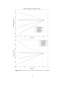
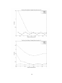
Figure 2.5: Results for All Sizing Methods and PDA, 100 to 150 microns, 0mm Plane
The results in Figure 2.5 show that the histogram for the three point Gaussian method matches
best with the PDA measurements in the range from 100 microns to 150 microns. This range
corresponds to approximately 4.2 to 6.25 pixels diameter in consideration of the overall
magnification factor of 24 microns per pixel. The three point Gaussian method follows the PDA
trend closely, exhibiting a correlation coefficient of 0.9571.
The four point Gaussian and
continuous four point Gaussian algorithms exhibit a bias toward higher diameters as compared to
PDA measurement. The correlation coefficients for the four point Gaussian, continuous four
point Gaussian, and the continuous least squares are 0.7916, 0.4130, and 0.4144, respectively for
the 0mm plane. The continuous least squares pdf exhibits a high degree of noise over this range
of diameter measurement, which stems from the low number of relative particles successfully
detected.
The histograms for the positive and negative 4mm displacement (measured from the center of the
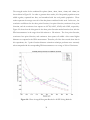
spray) are shown below in Figures 2.6 and 2.7. The results in Figures 2.6 and 2.7 also show that
the histogram for the three point Gaussian method matches best with the PDA measurements in
28
the range from 100 microns to 150 microns. The three point Gaussian method again follows the
PDA trend with a correlation coefficient of 0.9728. In the +4mm plane, the four point Gaussian
and continuous four point Gaussian algorithms exhibit the same trend as in the 0mm plane, a bias
towards the higher diameters. The correlation coefficients for the four point Gaussian, continuous
four point Gaussian, and the continuous least squares are 0.8904, 0.6692, and 0.5745, respectively
for the +4mm plane. The same general trends appear in the -4mm plane. but the histograms are
more erratic than in the +4mm plane results for the four point Gaussian and four point
continuous sizing algorithms. In the -4mm plane, the correlation coefficients for the three point
Gaussian, four point Gaussian, continuous four point Gaussian, and the continuous least squares
are 0.9761, 0.5558, 0.1957, and 0.5496, respectively. These results show that the 3 point Gaussian
performs much better in comparison to the PDA measurements than all of the other PIV sizing
methods.
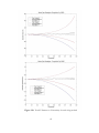
Figure 2.6: Histogram Results for - 4mm Spray Plane, All Sizing Methods
29
Figure 2.7: Histogram Results for + 4mm Spray Plane, All Sizing Methods
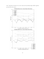
The histograms for the positive and negative 8mm displacement (measured from the center of the
spray) are shown below in Figure 2.8. Figure 2.8 shows the same general trends in the +/- 8mm
planes as seen in Figure 2.5 for the 0mm plane, except that the four point method performs better
than in the previously analyzed frames in the +8mm case. In the +8mm plane, the correlation
coefficients for the three point Gaussian, four point Gaussian, continuous four point Gaussian,
and the continuous least squares are 0.9697, 0.9642, 0.6892, and 0.3265, respectively. In the -8mm
plane, the correlation coefficients for the three point Gaussian, four point Gaussian, continuous
four point Gaussian, and the continuous least squares are 0.9699, 0.7605, 0.1798, and 0.3060,
respectively. The discrepancies between the 4 point, 4 point continuous, and least squares
methods are most likely due to the absence of sufficient points in the data to arrive at a solution
for diameter.
30
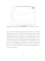
Figure 2.8: Histogram Results for +/- 8mm Spray Plane, All Sizing Methods.
31
The averaged results for the combined five planes (0mm, -4mm, -8mm, +4mm, and +8mm) are
shown below in Figure 2.9. In order to generate these results, all of the particle populations were
added together, separated into bins, and normalized with the total particle population. These
results represent the average across all of the data planes considered in this work. In this case, the
correlation coefficients for the three point Gaussian, four point Gaussian, continuous four point
Gaussian, and the continuous least squares are 0.9728, 0.8915, 0.5658, and 0.5883, respectively.
Figure 2.9 shows that the histogram for the three point Gaussian method matches best with the
PDA measurements in the range from 100 microns to 150 microns. The four point Gaussian,
continuous four point Gaussian, and continuous least squares all exhibit a bias toward higher
diameters as compared to the PDA measurement. Therefore, all of the above results show that in
this experiment, the 3 point Gaussian diameter estimation technique performs most accurately
when compared with the corresponding PDA measurements over a range of 100 to 150 microns.
Figure 2.9: Plane-Averaged Histogram Results for All PIV Sizing Methods
32
The performance of the three point Gaussian estimator is shown in more detail below in Figure
2.10.
Figure 2.10: Plane-Averaged Results for 3 Point Gaussian Method and PDA.
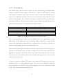
The particle population is also an important factor in this experiment. Table 2.1 below lists the
particle populations detected using the DPIV software for the 0mm plane. Table 2.1 shows that
the 3 point Gaussian produces a result at a rate approximately 99.71 percent of the detected
particle population, while the four point Guassian scheme produces results at approximately 19.40
percent. The 4 point continuous algorithm and the continuous least squares produce the lowest
success rates, at approximately 3.187 and 3.280 percent, respectively. Each method was performed
33
on the same images with identical image preprocessing procedures, and therefore the number of
particles fed to each algorithm for diameter estimation was identical.
Sizing Method
Particle
Population
(Number of
Successes)
554,497
107,868
17,726
21,187
Average
Successes Per
Frame
Total
Number of
Particle
Detected
556,111
556,111
556,111
556,111
3 point Gaussian
34.7
4 point Gaussian
6.7
4 point Continuous
1.1
Continuous Least
1.3
Squares
Table 2.1: Particle Population for Each Method, 0mm Plane
Success Rate
(%)
99.71
19.40
3.187
3.810
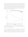
Table 2.2 below shows the correlation coefficient for each of the methods in tabulated form.
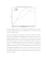
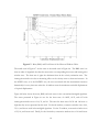
Figure 2.11 shows the results in Table 2.2 in graphical form.
Correlation Coefficient for Each Plane, Each Sizing Method
Plane (mm)
-8
-4
0
4
8
Plane Averaged
3 point
0.9699
0.9761
0.9571
0.9728
0.9697
4 point
0.7605
0.5558
0.7916
0.8904
0.9642
4 mod
0.1798
0.1957
0.413
0.6692
0.6892
0.9728
0.8915
0.5658
Table 2.2: Particle Population for Each Method, 0mm Plane
lsvl
0.306
0.5496
0.4144
0.5745
0.3265
0.5883
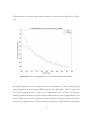
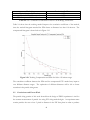
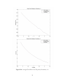
The results from Tables 2.1 and 2.2, along with Figure 2.11, show that only the 3 point method
succeeds at a reliable rate above 99 percent and exhibits a high value of the correlation coefficient
when compared to the PDA measurement over a diameter range from 100 to 150 microns. The
other conventional sizing methods did not perform adequately in this experiment, exhibiting
success rates ranging from 3 to 20 percent. The other methods also exhibited low values for the
correlation coefficient throughout the planes. The plane averaged correlation coefficient was
0.8915 for the 4 point Gaussian, 0.5658 for the continuous 4 point Gaussian, and 0.5883 for the
continuous least squares fit.
34
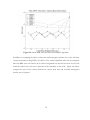
Correlation Coefficient vs. Plane for Conventional Sizing Methods
1.2
1
Correlation Coefficient
0.8
3 point Gaussian
4 Point Gaussian
Cont. 4 Point
Cont. LS
0.6
0.4
0.2
0
-10
-8
-6
-4
-2
0
2
4
6
8
10
Plane (mm)
Figure 2.11: Correlation Coefficient vs. Plane for Conventional Sizing Methods.
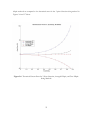
2.4.3
Average Diameter
In addition to histogram analyses, average diameter calculations provide another comparison tool
between the PIV and PDA diameter measurement techniques. The 3-D isosurface plot for the
average diameter for all of the spray planes is shown below in Figure 2.12. Figure 2.12 was
generated using the 0mm, +4mm, and +8mm results for the 3 point Gaussian sizing scheme and
reconstructing a volume using Tecplot 10. The data from each plane was scanned and counted
into 16 pixel bins with 50 percent overlap. The grid spacing in Figure 2.12 is 8 pixels, which allows
a grid of 32X32X5 for the entire volume. The average diameter was calculated assuming spherical
particles. Figure 2.12 was generated in Tecplot using isosurfaces between values of 54, 63, and 72.
The results in Figure 2.12 were smoothed for 3 passes using the built-in smoothing functionality of
Tecplot 10.
35
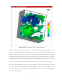
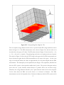
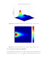
Figure 2.12: 3-D Isosurface Plot of Average Diameter
In Figure 2.12, the spray is located at (X,Y,Z) = (120,0,256). Figure 2.12 shows clearly shows the
volume reconstruction of the spray. The ligament can be clearly seen at in the bright green area.
Figure 2.12 shows that the larger particles are located near the ligament, and the average particle
diameter decreases as the distance from the spray increases. Since this analysis allows the complete
reconstruction of the entire volume, y plane slices may be extracted from the volume in order to
compare the average diameter at a certain height above the spray with the PDA measurements.
The slice of the reconstructed volume at an exact height of 15.4 mm is shown below in Figure
2.13. This elevation was located at 61.3097 pixels below the top of the spray images, or at an
elevation in the z plane of 194.69 pixels. The magnification used to find the corresponding region
was 79.1 microns per pixel.
36
Figure 2.13: Corresponding Slice Height in 3-D.
The out-of-plane average diameter results for the 3 point Gaussian PIV sizing method are shown
below in Figure 2.14. The PDA measurement is also shown in Figure 2.14, and was taken at an
elevation above the spray of 15.4mm. The PIV planes shown in Figure 2.14 are located at z = 16,
z = 32, z = 48, and z = 64 pixels. The grid spacing used in the out-of-plane results was 16 pixels.
The results in Figure 2.14 show that the PIV sizing results agree with the PDA measurement, are
about 40 microns higher than the PDA measurement in the center of the spray. On the outer
edge of the analyzed domain, the values are approximately 10 to 20 percent higher than the PDA
measurement. This discrepancy can be explained by the design of the experiment, which did not
allow the PIV system to detect particles smaller than 2 pixels. The previous histogram analysis
shows that the 3 point Gaussian method detects no particles below the 44 micron range.
Therefore, the average diameter detected by the 3 point Gaussian cannot be less than 44 pixels.
On the other hand, the PDA can resolve down to 1.4 microns in diameter.
The PDA
measurement accounts for all particles above 2 microns in diameter, while the PIV system used in
37
this experiment could only resolve 24 micron particles or greater. The mismatch between the
resolvable diameters results in the discrepancy between the two systems. The units in Figure 2.14
are average diameter in microns.
Figure 2.14 shows that the 3 point Gaussian fit overestimates the average diameter in comparison
to the PDA measurement. In the matching ranges, the PDA reaches a maximum level of 40
microns. The PIV values do not drop below 50 microns. Therefore, the PIV error ranges from
25% of the PDA to around 1000% in the center of the flow. The reason for this discrepancy,
again, is the inability of the PIV 3 point method to resolve diameters below 25 microns in
diameter. Even though a population of 25 micron particles exists in the data, the data shown in
Figure 2.14 is the average particle diameter passing through bins of 16 pixels square, or 1.6 square
millimeters. A bin size of 1.6 square millimeters is more than enough to capture particles of
several sizes in this experiment. This means that for every 25 micron particle that passes through
the center at 15.4mm above the spray, a larger particle traverses the same area within the entire
data set. Therefore, the PIV method cannot produce results in this analysis for diameters less than
25 pixels at the minimum under ideal bin selection criteria, while the PDA measurement can
resolve down to 1.4 microns. Therefore, due to the limitations of the PIV method, this analysis
cannot produce a viable comparison between the PDA and PIV methods for this data set.
38
Figure 2.14: PDA and 3 Point Gaussian PIV Average Diameter, z = 15.4mm
39
2.4.4
PTV-Corrected Histograms
PTV was performed on the spray data for the 0mm plane case using the 3 point Gaussian sizing
method. The PTV method used in this portion of the work was the Basic Trajectory option in
Flow-IQ v2.2. Histograms were generated for the tracking, the 3 point fit, and the compensated
tracking algorithm. The PTV compensated histogram was obtained by subtracting the tracking
algorithm from the overall 3 point Gaussian results. The tracking histogram was generated by
histogramming the average diameter of each tracked particle. The average diameter for a tracked
particle was calculated by using all of the occurrences of the particle throughout the data files.
Most of the particles in this study were tracked through only two frames. The results for the 3
point Gaussian fit, the particle tracking, and the PTV compensated histograms are shown below in
Figure 2.15.
Figure 2.15: Total Population Histograms for 3 Point Guassian, Tracking, and PTVcompensated methods, Spray 0mm plane.
40
Figure 2.15 shows that approximately 80 percent of the particles detected at the 25 and 44 micron
points were tracked using PTV. Approximately half of the particles from the 50 to 90 micron
range were tracked between frames. Therefore, the compensation using PTV decreases the overall
population bias towards the lower diameters for the 3 point Gaussian method. In order to
compare the methods to the PDA measurement, probability density functions were generated by
dividing the populations shown in Figure 2.15 with the total population for each corresponding
method. These results are shown below in Figure 2.16.
Figure 2.16: PDA, 3 point Gaussian, PTV, and PTV-compensated PDF’s, 0mm plane
Figure 2.16 above shows that the PTV and PTV-compensated pdf’s are much closer to the PDA
measurement than the full 3 point Guassian results. The correlation coefficients with the PDA
measurement for each of the methods shown in Figure 2.16 are listed below in Table 2.3.
41
Method
Correlation Coefficient
3 Point Guassian (Full Results)
0.1465
Tracked 3 Point Gaussian
0.1099
PTV-Compensated 3 Point Gaussian
0.1677
Table 2.3: PTV Correlation Coefficients for Full Range Results, 0 mm Plane
The correlation coefficient for the PTV-compensated algorithm is 14.5% higher than the
correlation coefficient of the 3 point Gaussian sizing method alone. The PTV-compensated
comparison with the PDA sizing method is shown in greater detail in Figure 2.17.
Figure 2.17: PTV-compensated and PDA histograms, 0mm plane
Figure 2.17 shows that the PTV compensated method significantly improves the estmation of
diameter population at the lower diameters. However, the correlation coefficient is still very low,
due to the inability of the 3 point method to resolve diameters smaller than 25 microns.
Therefore, the methods were also analyzed over the 100 to 150 micron range, as in the previous
sections. The histogram results for the 100 to 150 micron diameter range are shown below in
Figure 2.18. Figure 2.18 shows the total population for the PIV/PTV methods and the probability
density functions for the PIV, PDA, and PTV methods. Figure 2.18 suggests that the PTV 3 point
42
Gaussian method improves the correlation of the PIV method with the PDA measurement. A list
of the correlation coefficients over the 100 to 150 micron range is given in Table 2.4.
Figure 2.18: Population for PIV/PTV methods and PDF’s for PIV, PDA, and PTV
43
Method
Correlation Coefficient
3 Point Guassian (Full Results)
0.9571
Tracked 3 Point Gaussian
0.9759
PTV-Compensated 3 Point Gaussian
0.9558
Table 2.4: PTV Correlation Coefficients for 100 to 150 um Range, 0 mm Plane
Table 2.4 shows that the tracking method improves the correlation coefficient of the method,
since the tracked histogram matched the PDA better at diameters less than 110 microns. The
compensated histogram is shown below in Figure 2.19.
Figure 2.19: Tracking Compensation and PDA for 100 to 150 micron range.
The correlation coefficient between the PDA and the compensated PTV method may improve
over different diameter ranges. The exploration of different diameters will be left to future
researcher in the particle sizing arena.
2.5
Conclusions and Future Work
The particle sizing portion of this work showed that the design of DPIV experiments is vital for
the accurate measurement of particle size using PIV sizing methodologies. An experiment must
contain particles that are at least 3 pixels in diameter in the PIV data plane in order to produce
44
accurate results. Therefore, the minimum suggested particle diameter for sizing with PIV methods
is approximately 3 pixels. This conclusion is in agreement with the errors reported in Brady et al.
(2002), which showed that at diameters less than 3 pixels, the conventional PIV sizing methods
exhibit increasing error as particle diameter decreases. The spray results analyzed in this work did
not take this criterion into consideration at the time of data acquisition, and only portions of the
analyzed data were accurate. Therefore, it is the conclusion of this work that PIV experiments that
include sizing as a project goal should be designed with sufficient magnification to provide a
minimum of 3 pixels diameter for all particles the experimenters wish to size. This means that the
burden of producing accurate sizing results depends heavily on the appropriate setup and design of
the PIV experiment. New spray experiments are underway to test this criterion, and preliminary
results show that experiments with sufficient magnification produce results that match closely with
PDA measurements across the entire range of particle diameters. The PTV method has shown
initial promise in improving the correlation coefficient of PIV sizing methodologies with the
traditional PDA methods. Future work should focus on the improvement of the PTV-corrected
method for PIV particle sizing.
The spray sizing analysis completed in this work should be extended to further experiments with
adequate optical design to perform PIV average diameter analysis. This work showed that the
optimal design should magnify all desired particles to a minimum of three pixels diameter in order
to provide accurate spray sizing results. The new elliptical sizing methods should also be tested on
real data in order to determine their performance in real-world experiments.
2.6
Summary of Original Contribution
The original contribution of this work is the application of the sizing methods developed by
previous researchers to an entire set of spray atomization data. No new sizing methods were
developed or used in the spray sizing portion of this work. The histogram analysis found that the
3 point Gaussian sizing method exhibited a correlation coefficient of up to 0.9728 when compared
to the PDA method over a range of 100 to 150 microns in diameter (4 to 7 pixels in diameter).
Although the PIV average diameter results in this section do not agree with the PDA
measurement, several important observations were made from this analysis. The PIV experiment
must be designed to have sufficient magnification, such that the particles the experimentor(s) wish
45
to size are greater than 3 pixels in diameter in the PIV data. Over the detectable range of PIV
sizing (greater than 3 pixels in diameter), the PIV sizing method performed with a correlation
coefficient of up to 0.9728 when compared statistically to the PDA sizing method. Therefore, the
major finding of this work is the conclusion that PIV sizing experiments must be carefully
designed to provide the necessary particle size for comparable results to PDA measurements. This
work was performed as a validation of the particle sizing methodologies as an application of the
new sizing software in a real experiment. The only original algorithm in this work is the PTVcorrected method for particle sizing, which will be further developed by future researchers.
46
Chapter 3
3
ELLIPTICAL PARTICLE SIZING METHOD
The purpose of this chapter is to explore the development of a novel elliptical sizing algorithm
developed by the author. Previous sizing methodologies have made the assumption that particles
are spherical in shape, and present a circular profile in DPIV data. In some applications, this
assumption can be justified. However, in several applications, such as spray atomization, droplets
or seed particles deform and may present elliptical profiles in DPIV data. Therefore, this work
explores the development of an elliptical sizing method that is not limited to circular profiles.
Monte Carlo simulations were also performed in order to validate the performance of the method
on simulated DPIV data.
3.1
Introduction
In this work, an elliptical particle sizing technique was developed in order to overcome the
assumption that all particles in a flow field are spherical. The assumption of spherical particles
introduces error into the measurement of diameter using the conventional PIV sizing schemes
presented above in Chapter 2. In order to create an elliptical particle, the intensity in the x and y
directions were assumed to be jointly Gaussian, identically independent random variables.
Two random variables x and y are considered Jointly Gaussian is their joint pdf is defined as (Stark
and Woods, 1986):
f XY ( x, y ) =
1
2πσ xσ y 1 − ρ 2
2
⎛
⎧
&⎞ 2
(x − X&&&)( y −Y&&&)+⎛⎜ y −Y&&&⎞⎟ ⎫⎪ ⎞⎟
⎜
−1 ⎪ ⎛ x − X&
⎜
⎟
ρ
2
−
⎨
⎜
⎜
⎟
2
⎜ σ y ⎟ ⎬ ⎟⎟
σ xσ y
⎜ 2 (1− ρ ) ⎪ ⎝ σ x ⎠
⎠ ⎪⎭ ⎠
⎝
⎩
⎝
e
(Eq. 3.1)
where σx is the standard deviation in the x direction, σy is the standard deviation in the y direction,
µx is the mean of the x variable , µy is the mean of the y variable, and ρ is the correlation
coefficient between the x and y random variables.
47
When the x and y are considered to by identically independent random variables (ρ = 0), equation
3.1 reduces to:
f XY ( x, y ) =
1
2πσ xσ y
2
⎛ ⎧
&⎞2 ⎛ y −Y
&
&
&⎞ ⎫⎪ ⎞⎟
⎜ −1⎪ ⎛ x − X&
⎟
⎜
⎟
⎜
+
⎬⎟
⎜ ⎨⎜
⎟
⎜ 2 ⎪ ⎝ σ x ⎠ ⎜⎝ σ y ⎟⎠ ⎪ ⎟
⎭⎠
⎝ ⎩
e
(Eq. 3.2)
This equation describes an elliptical Gaussian curvature, whose semimajor axis is related to the
greater of σx or σy, and whose simeminor axis is related to the lesser of σx or σy. The semimajor
and semiminor axes are the particle width in the x and y direction. An ellipse is shown below in
Figure 3.1 (Harris and Stocker, 1998).
Figure 3.1: Diagram of
an ellipse.
Brady et. al. (2004) examined particles using the assumption that particle distributions were
normally distributed i.i.r.v.’s with σx equal to σy, which produces a circular distribution as shown
below in Figure 3.2.
48
Figure 3.2: Jointly Gaussian IIRV’s with σx = σy.
For a circular particle, Brady et. al. showed that for circular particles, σx and σy are given by the
following equations.
xc = xo +
ln ao −1 −ln ao +1
2(ln ao −1 +ln ao +1 −2 ln ao )
(Eq. 3.3)
yc = yo +
ln ao −1 −ln ao +1
2(ln ao −1 +ln ao +1 −2 ln ao )
(Eq. 3.4)
σ2 =
ln ao +1 − ln ao
( xo − xc ) 2 − ( xo +1 − xc ) 2
(Eq. 3.5)
d = 2σ
ai = I oe
−
( xi − xc ) 2
2σ 2
49
(Eq. 3.6)
(Eq. 3.7)
Where a0 and a0+1 are the intensities at the center pixel and the pixel to the right of the center pixel,
x0 and x0+1 are the pixel positions of the center and right pixel, x0 and x0+1 are the pixel positions of
the center and right pixel, respectively, and d is the estimated diameter of the particle.
For an elliptical particle the above equations are reduced to the following equations for σx, σy, b,
and c, where b and c are the semimajor and semiminor axes.
σ x2 =
σ y2 =
ln a xo +1 − ln a xo
( x xo − xc ) 2 − ( x xo +1 − xc ) 2
ln a yo +1 − ln a yo
( y yo − yc ) 2 − ( y yo +1 − yc ) 2
(Eq. 3.8)
(Eq. 3.9)
b = 2σ x
(Eq. 3.10)
c = 2σ y
(Eq. 3.11)
Figure 3.3 below shows some example plots of jointly Gaussian i.i.r.v.’s with various values of σx
and σy. Using these equations, elliptical particles can be accurately sized. This distribution can be
used to size particles that do not exhibit a circular shape, such as elliptical droplets, streaked
particles, particles detected in regions of high background noise or non-symmetric crosscorrelation distribution peaks.
50
Figure 3.3: Jointly Gaussian IIIRV’s with various values of σx and σy.
Errors were calculated in this work as the difference between the actual area of the particle and the
measured area of the particle. The area of an ellipse is simply πbc, where b is the semimajor axis
of the ellipse, and c is the semiminor axis of the ellipse. The eccentricity of an ellipse, which
describes the shape of the ellipse, is defined below in equation 3.11.
b2
e = 1− 2
c
(Eq. 3.12)
The eccentricity varies from 0 to 1 for an ellipse, since the semiminor axis is by definition less than
the semimajor axis.
3.2
Elliptical Particle Sizing Scheme Methods and Materials
A theoretical analysis of the elliptical sizing method was performed. Monte Carlo simulations of
the performance of the method will be left to future research.
3.3
Elliptical Particle Sizing Results
The theoretical advantages of using an elliptical particle sizing algorithm are explored in the
following section. These results provide the basis for future work in the development of elliptical
51
sizing techniques. Section 3.3.2 presents the experimental portion of this work, which consists of
Monte Carlo simulations in order to determine the performance of the elliptical sizing method in
simulated data.
3.3.1
Theoretical Foundations
The conventional 3 point sizing method takes only the x direction into account when sizing
particle. This procedure can certainly be improved by the addition of a y component to the
diameter measurement. The particle may either as a true ellipse, or as a sphere by averaging the x
and y diameter measurements. This analysis assumes that the ellipse is axisymmetric around the x
and y axes.
The error associated with the measurement, in this work, is considered as the percent difference in
area of the measured particle as compared to the actual area of the particle. The percent difference
is defined below in Equation 3.12.
% err =
Ameas − Atrue
Atrue
(Eq. 3.13)
The area of the conventional method is simply πd2, where d is the measured diameter of the
particle in the x direction. The theoretical error of the traditional method when x is the semimajor
axis of the ellipse is given by Equation 3.13, which reduces to Equation 3.14.
e% xmaj =
πb 2 − πbc
πbc
e% xmaj =
b
−1
c
(Eq. 3.14)
(Eq. 3.15)
The theoretical error of the traditional method when x is the semiminor axis of the ellipse is given
by Equation 3.15, which reduces to Equation 3.16.
e% x min =
πc 2 − πbc
πbc
52
(Eq. 3.16)
e% x min =
c
−1
b
(Eq. 3.17)
The theoretical error of the averaged elliptic sizing method, where the diameter is considered to be
the average of the semiminor and semimajor axes, is given by Equation 3.17. This equation
reduces to Equation 3.18.
⎛b+c⎞
π⎜
⎟ − πbc
2 ⎠
⎝
=
πbc
2
e% xavg
e% xavg =
b
c 1
+
−
4c 4b 2
(Eq. 3.18)
(Eq. 3.19)
The theoretical error of the true elliptic sizing method, where the area is defined as πbc, is
identically zero.
Figure 3.4 below shows the theoretical error introduced by using only the x direction as a
measurement of an ellipse with varying eccentricity. Eccentricity is defined as the square root of
one minus the square of the ratio of the semiminor axis to the semimajor axis.
Figure 3.4: Theoretical Area Calculation Error vs. Eccentricity for Conventional Sizing Method
53
Figure 3.4 above shows that, theoretically, the error introduced by measuring the diameter with
only the x information diverges as the eccentricity increases. At an eccentricity of 0.866, the error
is 100 percent for the case of an x semimajor axis, and -50 percent for the case of a y semimajor
axis. This analysis was performed in order to demonstrate the need for improvement in the three
point Gaussian sizing method. Another presentation of the theoretical error introduced by the 3
point Gaussian sizing method is shown below in Figure 3.5. These errors are plotted as a function
of axis ratio for the case of x and y semimajor axes.
Figure 3.5: Theoretical Error vs. Axis Ratio for 3 point Gaussian Sizing Method
Figure 3.5 above is more intuitively obvious, as the error diverges when the discrepancy between
the semimajor and semiminor axes increases.
The novel sizing methods presented in this work are the averaged elliptic and true elliptic sizing
methods.
The averaged elliptic method uses the average of the two axes to arrive at a
measurement diameter. The true elliptic method sizes a particle using the two independent
measurements, thus forming a true ellipse. The theoretical error for the averaged elliptic and true
54
elliptic methods are compared to the theoretical error for the 3 point Gaussian sizing method in
Figures 3.6 and 3.7 below.
Figure 3.6: Theoretical Percent Error for 3 Point Gaussian, Averaged Elliptic, and True Elliptic
Sizing Methods
55
Figure 3.7: Theoretical Percent Error for 3 Point Gaussian, Averaged Elliptic, and True Elliptic
Sizing Methods
The above results show that the averaged elliptic sizing method, in theory, reduces the error in the
measurement by 5 to 10 times, maxing at 12.5 percent at an eccentricity of 0.866 and an axis ratio
of 0.5. It is also interesting to note that the averaged elliptic sizing method exhibits the same error
whether the x-axis is the semimajor axis or the semiminor axis. Therefore, the true elliptic and
averaged elliptic sizing methods exhibit the ability to correct for non-spherical particles within a
flowfield, while the conventional 3 point Gaussian exhibits an error that diverges greatly with
eccentricity. However, the theoretical calculations presented above do not account for the error
introduced by pixel discretization. Future work in this area will include Monte Carlo Simulations
of the elliptical sizing algorithm and its performance comparison to traditional Gaussian particle
sizing methodologies.
3.3.2
Experimental Analysis
Monte Carlo Simulations were used in order to characterize the performance of the elliptical sizing
method on simulated PIV data. A total of 5000 images were generated with particles with
56
eccentricities varying from 0 (circular) to 0.8660 (50 percent difference between the semimajor and
semiminor axes).
Two example images are shown below in Figure 3.8. The generated images
were 32 X 32 pixels square and the center of the particle was forced to be located at (x,y) =
(7.25,7.25) in order to fix the particles within the image.
Figure 3.8: Sample Monte Carlo Simulation Images.
The images used in this experiment were generated using MatLAB 6.0. The profiles were assumed
to be elliptical Gaussian profiles as developed in the introduction of this chapter. The pixel values
were obtained by integration of the elliptical Gaussian profile over the pixel area in order to
simulate the optics of a CCD device. The traditional and novel elliptical sizing methods were
performed on each image, and the error was calculated according to Equation 3.13. The results
obtained from this analysis follow.
In order to test the methods on a basic level, circular particles were generated in order to provide a
baseline method to ensure that the different methods developed in this work agreed with the
traditional 3 point Gaussian method. The total error in the diameter measurement is shown below
in Figures 3.9 and 3.10. To generate Figure 3.10, the error values shown in Figure 3.9 were
averaged over 250 measurements, which generated 20 data points over the data range from 2.8
pixels to 5.6 pixels in steps of 0.14 pixels.
57
Figure 3.9: All Data Points for Eccentricity = 0, Diameter range 2.8 to 5.6 pixels
58
Figure 3.10: Averaged Total Error over 250 points, Eccentricity = 0.
59
Figures 3.9 and 3.10 above show that the 3 point Gaussian, averaged elliptic, and true elliptic sizing
methods perform with a correlation coefficient of 1.00. The correlation coefficient is unity
between all of the methods for the case of no eccentricity. The absolute and percent error shown
in Figures 3.9 and 3.10 agree with previous results obtained by Brady et al. (2002) in their study of
the 3 point Gaussian sizing scheme. Since the zero eccentricity case has been established, the
performance of the various sizing methods are explored in the following paragraphs.
There are several ways to present the error analysis in this section. The first approach used to
determine the errors associated with the diameter measurement was to calculate the error in the x
and y diameters. For the 3 point Gaussian fit, the x diameter is the only calculated diameter, and
therefore this diameter is used as a comparison to the actual y diameter in this simulation. The
averaged elliptic method assumes a spherical shape with the average of the diameter in the two
directions. Therefore, for the averaged elliptic method, the average diameter was compared to the
actual diameter in the x and y directions. For the true elliptic fit, the corresponding diameters were
compared. The results from this analysis are shown below in Figure 3.11 and 3.12. The same
procedure for Figures 3.9 and 3.10 were used to generate these graphs. Figure 3.11 shows the
comparative absolute and percentage error in the x and y diameter measurements versus x
diameter, and Figure 3.12 shows the comparative errors in the x and y diameter measurements
versus eccentricity. For the images used to obtain these results, the x diameter was chosen at
random in a range from 2.8 to 5.6 pixels in diameter. The y diameter was held constant at 5.6
pixels in order to fix the eccentricity range from 0 to 0.8660.
60
Figure 3.11: Error in the x and y diameter measurements vs. x diameter
61
Figure 3.12: X and Y diameter vs. Eccentricity for each sizing method
62
Figures 3.11 and 3.12 above shows that the true elliptical sizing method exhibits a correlation
coefficient of 1.00 with the 3 point Gaussian in relation to x diameter. The averaged elliptic
method exhibits diverging error in the x and y diameter measurement as eccentricity increases.
This phenomenon should be expected, since the averaged elliptic method uses the average of the
two diameters and assumes a spherical particle profile. Therefore, when the x diameter is less than
the y diameter, the averaged elliptic method will overestimate the x diameter and underestimate the
y diameter. This behavior is clearly visible in Figures 3.11 and 3.12. The true elliptic sizing
method exhibits the lowest error in the y direction, since the true elliptic method is the only
method that performs a true sizing scheme in the y direction.
Figures 3.11 and 3.12 show the
behavior of each sizing method with respect to diameter and eccentricity. Figure 3.12 shows that
the true elliptical sizing method performs identically with the traditional 3 point Gaussian sizing
scheme in the x direction. However, the 3 point Gaussian method exhibits error that reaches a
level of -50% at an eccentricity of 0.8660, which corresponds to an axis ratio x/y of 0.50.
Another method for calculating the error associated with the various sizing methods is the area
estimation. In this section, the actual area was compared to the estimated area by the various
sizing schemes. Therefore, this section deals with the area in the projected area of a particle image
in DPIV data. The area error results from the Monte Carlo Simulations are shown below in
Figure 3.13. The error was plotted as a function of eccentricity. For the data shown in Figure
3.13, the x axis was considered to be the semimajor axis.
63
Figure 3.13: Area absolute and percent error for all sizing methods
64
Figure 3.13 shows that the pixel intensity discretization introduces significant error into the
measurement of particle area. The errors are higher than the theoretical errors by approximately
10 to 20 percent. However, the trends in Figure 3.9 agree with the theoretical findings in Section
3.3.1 for the averaged elliptic method. The true elliptic method exhibits higher error than the
traditional 3 point method for eccentricities less than 0.60. The error for the averaged elliptic
method is lower than the traditional 3 point Gaussian method by approximately 5% at an
eccentricity of 0.03. The error is decreased by using the averaged elliptic method by approximately
80 percent when compared to the traditional 3 point Gaussian method. These results show that
the averaged elliptic method performs the best out of the three methods tested in this section.
3.4
Conclusions and Future Work.
In this chapter, an elliptical sizing methodology was introduced and tested using Monte Carlo
simulations. These studies found that for particles of elliptical profile, the averaged elliptic method
performs the best in the measurement of particle area. The trends seen in the Monte Carlo
Simulations agree with the trends predicted by theory. Therefore, the elliptical sizing method has
been theoretically introduced and validated experimentally using Monte Carlo Simulations.
Future work in the particle sizing area should concentrate on the development of more adaptive
sizing algorithms that can dynamically adapt to size a given particle based on its intensity profile.
Monte Carlo simulations should be performed in order to confirm the theoretically-improved
performance of the elliptical sizing method. The next step in the evolution of the Gaussian sizing
methods is the development of a rotation for the elliptic Gaussian profile and conversion from the
pixel domain to a rotated pixel domain. This rotated elliptic Gaussian profile could accurately
detect particles that are deformed and not restricted to the normal Cartesian coordinate system.
This sizing scheme could either perform a brute force axis rotation, or utilize the assumption that
the intensity is jointly Gaussian and dependent with correlation coefficient ρ. New profiles could
also be explored for future sizing value with streaked particles. Two profiles of particular interest
are the log-normal normal independent (LNNI) and the Rayleight normal independent (RNI)
probability density functions. These functions are summarized below. These profiles, along with
rotation techniques, could provide a powerful tool for the estimation of diameter and particle
shape using PIV.
65
3.4.1
Log Normal / Normal Independent (LNNI) PDF.
For the LNNI probability density function, two random variables x and y were considered to be
independent random variables. The x r.v. was considered to be log-normally distributed with
standard deviation σx and mean value µx. The y r.v. was considered to be normally distributed
with standard deviation σy and mean value µy. For a log-normally distributed variable x, the pdf is
defined as follows:
f X ( x) =
1
σx
&⎞
⎛ ln( x ) − X&
⎟⎟
⎜⎜
⎝ 2σ x ⎠
2
e
2π
(Eq. 3.20)
For a normally distributed variable y, the pdf is defined as follows:
f Y ( y) =
1
σ y 2π
&
&⎞
⎛ y −Y&
⎟
⎜
⎜ 2σ y ⎟
⎠
⎝
2
e
(Eq. 3.21)
For independent r.v.’s, the joint pdf can be expressed as (Stark and Woods, 1986):
f XY ( x, y ) = f X ( x) * gY ( y )
Therefore, the joint pdf for an LNNI system can be written as:
f XY ( x, y ) =
1
2πσ xσ y
2
⎛ ⎧
&⎞ 2 ⎛ y −Y&
&
&⎞ ⎫⎪ ⎞⎟
⎜ ⎪ ⎛ ln( x ) − X&
⎟
⎜
⎟
⎜
+
−
⎬⎟
⎜ ⎨⎜
⎟
⎜ ⎪ ⎝ 2σ x ⎠ ⎜⎝ 2σ y ⎟⎠ ⎪ ⎟
⎭⎠
⎝ ⎩
e
(Eq. 3.22)
(Eq. 3.23)
where σx is the standard deviation of r.v. x, σy is the standard deviation for r.v. y direction, µx is the
mean of r.v. x , and µy is the mean of r.v. y.
Figures 3.14 and 3.15 below show the a 2-D probability density function with x as a log-normal
random variable with σx = 0.80 and µx = 1.00, and y as a Gaussian random variable with σy =
0.30 and µy = 0.00. The variables in these plots are assumed to be independent random variables x
and y. This pdf may prove to be extremely useful in simulating streaked particles. The parameters
σx and µx determine the skewness and length of the pdf’s “tail.” The parameters σy and µy can be
manipulated to simulate particles of larger diameter. This probability density function allows the
simulation of particles that exhibit skewness and streaking characteristics.
66
Figure 3.14: Log-Normal Surface Plot for σx = 0.80, σy = 0.30, µx = 1.00 , µy = 0.00
Figure 3.15: Log-Normal Contour Plot for σx = 0.80, σy = 0.30, µx = 1.00 , µy = 0.00
3.4.2
Rayleigh Normal Independent (RNI) PDF.
For the RNI probability density function, two random variables x and y were considered to be
independent random variables. The x r.v. was considered to be Rayleigh distributed with skewness
67
factor s. The y r.v. was considered to be normally distributed with standard deviation σy and mean
value µy. For a Rayleigh distributed variable x, the pdf is defined as follows:
x
f X ( x) = 2
s
⎛ x2
−⎜⎜ 2
⎝ 2s
e
⎞
⎟
⎟
⎠
(Eq. 3.24)
For a normally distributed variable y, the pdf is defined as follows:
f Y ( y) =
&
&⎞
⎛ y −Y&
⎜
⎟
⎜ 2σ y ⎟
⎝
⎠
1
2
(Eq. 3.25)
e
σ y 2π
For independent r.v.’s, the joint pdf can be expressed as (Stark and Woods, 1986):
f XY ( x, y ) = f X ( x) * gY ( y )
(Eq. 3.26)
Therefore, the joint pdf for an RNI system can be written as:
f XY ( x, y ) =
1
s 2σ y 2π
⎛ ⎧ 2
⎜ ⎪⎛ x
⎜ − ⎨⎜⎜ 2
⎜ ⎪⎝ 2 s
⎝ ⎩
e
2
&
&⎞ ⎫⎪ ⎞⎟
⎞ ⎛ y −Y&
⎟ ⎬⎟
⎟ +⎜
⎟ ⎜ 2σ ⎟ ⎟
y ⎠ ⎪
⎠ ⎝
⎭⎠
(Eq. 3.27)
Figures 3.16 and 3.17 below show the a 2-D probability density function with x as a log-normal
random variable with s = 6.00, and y as a Gaussian random variable with σy = 0.20 and µy = 0.00.
The variables in these plots are assumed to be independent random variables x and y. This
distribution may be useful in quantifying particles that are slightly streaked or skewed. The
parameter s determines the skewness of this distribution The parameters σy and µy can be
manipulated to simulate particles of larger diameter. This probability density function allows the
simulation of particles that exhibit noncircular or skewed profiles.
68
Figure 3.16: Log-Normal Surface Plot for σy = 0.20, µy = 0.00, s = 6.00
Figure 3.17: Log-Normal Contour Plot for σy = 0.20, µy = 0.00, s = 6.00
These probability density functions approximate the shape of a streaked particle, and therefore
may be of use in data recovery and high speed flow experiments. Future work should also include
69
the application of the elliptical sizing technique to the other methods, including the four point
Gaussian, continuous four point Gaussian, and least squares sizing methods.
3.5
Summary of Original Contribution
In this Chapter, the major original contribution is the development of a Gaussian particle sizing
method that is not limited to spherical particles.
experimental Monte Carlo simulations.
The method was confirmed with initial
The potential of this method is apparent from the
theoretical and experimental analysis presented in this chapter. The work on the development of
the elliptical sizing method opens a door for the application of the sizing methods to elliptical and
deformed seed particles in DPIV data sets, which represents a first next step in the development
of advanced particle sizing methods. The work presented in this chapter is intended as an initial
step for the continuation of the development of elliptical sizing algorithms.
70
Chapter 4
4
4.1
WALL SHEAR EXPERIMENTS
Introduction
A major aim of this work is to quantify the accuracy of wall velocity estimation using DPIV.
Velocity measurement error for DPIV has been quantified in the past (Huang et al., 1997). Even in
the presence of strong velocity gradients the accuracy of the velocity measurements is better than
0.1 pixels (px) for state-of-the-art systems. However, in the case of wall-bounded flows, crosscorrelation induced spatial averaging effects can significantly affect the measurement due to very
strong localized shear rates. The particle pattern displacements are determined with sub-pixel
resolution from the cross-correlation peak for each interrogation window, using a Gaussian fit that
is applied to the correlation coefficient matrix. Detailed analyses of these methods can be found in
several of the referenced papers in this work (Marxen et al., 2000, Meunier and Leweke, 2003,
Raffel et al., 1998, Wereley and Meinhart, 2001, Nogueira et al., 1999). For near wall measurements
the cross-correlation signal to noise ratio is often compromised by reduced seeding density
compared to the outer flow.
Evaluation of near-wall velocities from experimentally determined DPIV flow fields is most
affected by the effect of spatial averaging due to window interrogation size. This is particularly true
as the shear rate increases, which effectively skews the correlation matrix, the consequence of
which is the inability of the conventionally utilized Gaussian three-point estimator to accurately
determine the true displacement at the center of the window (Marxen et al., 2000). The signal is
dominated by the flow away from the boundary due to higher velocities and better seeding, density
causing a biasing of the displacement estimation. Only the effect of velocity gradient on the
measurement accuracy will be considered here, as the near wall seeding is a system-dependent
parameter.
71
4.2
Wall Shear Methods and Materials
Monte Carlo Simulations were performed in order to test the accuracy of several DPIV algorithms
when measuring wall shear.
One hundred artificial Couette flow images were created using in-
house artificial image generation software for each shear rate studied in this work. In order to
compare the error associated with DPIV measurements of velocity under velocity gradients, low
shear rate images were generated in order to create centerline displacements of 0.1 to 0.5 pixels in
0.1 pixel increments. The shear rates used to produce these centerline displacements were 0.025,
0.050, 0.075, 0.100, and 0.125 pixels per pixel. Shear rates of 0.0625, 0.125, and 0..25 pixels per
pixel were examined in order to determine the effects of increased shear rate on DPIV
performance. The artificial images were then analyzed using several different DPIV methods.
The methods tested in this work were no discrete window offset DPIV (single-pass DPIV), multigrid DPIV (traditional DPIV algorithm), and a novel ultra-DPIV method developed in our
laboratory. After the artificial data was analyzed using each DPIV method, the mean, RMS, and
total errors were calculated for each case. The flow-field used in these experiments is shown
below in Figure 4.1.
Figure 4.1: Artificial Image Diagram for Wall Shear Experiments
In order to obtain the desired shear rates, maximum velocities of 16, 32, 64, 128, and 256 were
used in the artificial image generation software.
72
For the low shear portion of this work, maximum velocities of 6.4, 12.8, 19.2, 25.6, and 32 were
used to yield shear rates of 0.025, 0.050, 0.075, 0.100, and 0.125. These shear rates were targeted
in order to produce centerline displacements ranging from 0.1 to 0.5 pixels for error analysis and
comparison to traditional PIV error uniform displacement results.
The tracking portion of this work utilized the Hybrid PTV algorithm available in Flow-IQ v2.2 to
calculate the error associated with particle tracking in a shear flow. A search radius of 3 pixels was
used in conjunction with No Discrete Window Offset PIV and 3 point Guassian sizing to track
the particles in the artificial Couette images. The velocities from PTV were then compared to the
known velocity at the particle’s y postion obtained from the sizing algorithm and errors were
plotted as a function of displacement for the low shear rates discussed above.
4.3
Wall Shear Results
The first goal of the wall shear portion of this work was to characterize the expected error
associated with wall velocity measurements using DPIV.
The wall shear characterization
performed in this work was divided into two sections, a high shear section and a low shear section.
The high shear section studied Couette flows with velocity gradients up to 1 pixel per pixel. The
low shear section targeted shear rates that would produce centerline displacements of 0 to 0.5
pixels in 0.1 pixel increments.
4.3.1
Low Shear Rate Study
The shear rates examined in the high shear portion of this work were 0, 0.025, 0.05, 0.075, and
0.100, and 0.125 pixels per pixel shear rate. These shear rates produced the desired centerline
displacement of 0 to 0.5 pixels at the first measurement point. The images generated for this work
had zero background noise in order to isolate the effects of shear rate on the velocity error.
Procedures identical to the high shear rates were used for the analysis of the low shear images.
Errors were plotted to compare the performance of the various methods at different window
sizes. Figure 4.2 below shows the total error for all methods studied in this work with a starting
interrogation window of 64 pixels.
Figure 4.2 shows that the NDWO method has the highest error at a starting interrogation window
of 64. The conventional multigrid method exhibits a spike in bias and rms error at centerline
73
displacements of 0.4 and 0.5 pixels. The DADPIV method, however, performs consistently over
the range of displacements shown in Figure 4.2. The DADPIV and multigrid methods exhibit
similar behavior at displacements ranging from 0 to 0.3 pixels.
Figure 4.2: Total Error for all DPIV methods, Window 64
Figure 4.3 below shows the total errors for a starting interrogation window of 32 pixels.
74
Figure 4.3: Total Error for all DPIV methods, Window 32
According to Figure 4.3, the multigrid and DADPIV algorithms have nearly identical performance
over the range 0 to 0.5 pixels for an initial interrogation window size of 32 pixels. As in Figure 4.2,
the RMS errors are an order of magnitude less than the associated mean errors. The NDWO
method also exhibits a much higher error than the multigrid or DADPIV algorithms. Figure 4.4
below shows the total errors for an initial interrogation window of 16 pixels.
75
Figure 4.4: Total Error for all DPIV methods, Starting Window 16.
For an initial interrogation window size of 16, the multigrid and DADPIV methods have a higher
error than the NDWO method, except at the displacements of 0.4 and 0.5, where all three
methods have similar performance.
The above results suggest that for measurement of wall velocity in shear flows that exhibit
relatively low velocity gradients, the initial interrogation window size plays a major role in the error
associated with the measurement.
The NDWO offset case represents the first pass in the
multigrid and DADPIV methods. The errors shown in Figures 4.2 through 4.4 were calculated
without taking the absolute value. Therefore, as initial interrogation window size increases, the
first pass of all of the DPIV algorithms studied in this work overestimates. At an interrogation
window size of 64, this overestimation reaches the level of 2 pixels. Since the multigrid and
DADPIV methods exhibit a lower true error than the NDWO method, the refining passes in both
the multigrid and the DADPIV methods must correct for the overestimation in some manner.
The multiple pass methods can only correct by 0.5 pixels in each successive pass.
If the
overestimation is greater than 0.5 pixels, the multiple pass algorithms may not be able to correct
for such an overestimation.
76
4.3.1.1
Comparison to Uniform Displacement Measurements
The wall shear results were compared to uniform displacement results in order to determine the
difference between the measurement error in wall shear and the error associated with uniform
displacement, which has been well documented.
Figure 4.5 below shows the uniform
displacement error in comparison to the wall shear velocity error for a starting interrogation
window size of 32 pixels.
Figure 4.5: Wall Shear Error Compared to Uniform Displacement Error.
Figure 4.5 shows that the error for the shear flows studied in this work are much higher than the
error associated with uniform displacement. The errors for uniform displacement agree with the
error reported by Huang et al. (1997). Therefore, the introduction of velocity gradients into a flow
significantly increases the error associated with DPIV velocity measurements.
77
4.3.1.2 Tracking Results
The artificial images used in the above analyses were also processed using the Hybrid Particle
Tracking Velocimetry routine available in Flow-IQ v2.2. Unlike the PIV results, the tracking
results produce a continuous velocity field. The errors at each y location were computed from the
output of the Hybrid PTV algorithm. The shear rates analyzed were 0.025, 0.050, 0.075, 0.100,
and 0.125 pixels per pixel. The total number of particles successfully tracked for each shear rate is
listed below in Table 4.1. These results were obtained using a starting interrogation window of 16,
which yielded approximately 5 to 6 particles per interrogation window.
Shear Rate (px/px)
Number of Particles Tracked (per 100 frames)
0.025
7068
0.050
4017
0.075
2748
0.100
1952
0.125
1667
Table 4. 1: Tracked Particle Populations for Each Shear Rate
The 16 starting interrogation window can only reliably resolve up to approximately 4 pixels
displacement. For the higher shear rates, an increasing number of particles are in regions where
accurate PIV measurement is impossible with a starting window of 16 pixels. Therefore, the
number of tracked particles decreases with increasing shear rate.
Since the particle tracking process produces a continuous velocity field, the error can be plotted as
a function of the centerline velocity. In order to compute this error, the velocity calculated by the
algorithm was compared to the known velocity at the particles distance from the top of the image.
The absolute value of the difference between the calculated and expected velocity values was used
as the local error in this study.
In order to compare the Hybrid PTV results to the traditional PIV methods, the errors were
calculated for the 0 to 1 pixel displacement range. The total error was defined by setting bins
around pixel markers for the PTV method, and averaging the error for the measurements within
the bin. The results are shown below in Figure 4.6.
78
Figure 4.6: Total Error for all PIV methods and PTV
Figure 4.11 above shows that the PTV method performs much better than the PIV methods in the
estimation of velocity in shear flows. The error for the PTV method is approximately half that of
the PIV methods at corresponding displacements. A larger number of images must be analyzed in
order to improve this assessment, however, since the particle populations at higher shear rates are
relatively low and unreliable.
4.3.2
High Shear Rate Study
The shear rates examined in the high shear portion of this work were 0.0625, 0.125, 0.25, 0.50, and
1.00 pixels per pixel shear rate. The images generated for this work had zero background noise in
order to isolate the effects of shear rate on the velocity error. The no discrete window offset case
stands as the control case for these experiments.
79
For the no discrete window offset (NDWO) case, the interrogation windows were 64, 32, and 16.
In this case, there were no consecutive passes performed in order to refine the velocity
measurement. The results for the NDWO case are shown below in Figure 4.7.
80
Figure 4.7: Mean, RMS, and Total Error for No Discrete Window Offset.
The trends seen in Figure 4.7 are the same as the trends seen in Figure 4.6. The RMS error is at
least an order of magnitude less than the mean error at corresponding shear rates and interrogation
window sizes. The shear rate is again the dominant factor in the velocity estimation error. The
interrogation window size has an increasing effect on the velocity error as shear rate increases. In
the NDWO case, as in the DADPIV case, the error associated with the measurement increases
dramatically for every shear rate when the 16 window nears the maximum resolvable displacement
of 4 pixels displacement.
Figure 4.8 below shows the mean, RMS, and total error for the conventional multigrid algorithm.
The errors presented in Figure 4.6 are for the shear rates of 0.0625, 0.125, and 0.25 with
interrogation window sizes of 64, 32, and 16. The error for shear rates of 0.50 and 1.00 were so
high that they are not presented in this work. For the 64 window, consecutive window sizes of 64,
32, 16, and 8 were used in the multigrid algorithm. For the 32 window, consecutive window sizes
of 32, 16, and 8 were used. Finally, for the 16 window, consecutive window sizes of 16 and 8 were
81
used. This pattern of window sizes was also used with the dynamically-adaptive DPIV algorithm
presented later in this section.
82
Figure 4.8: Mean, RMS, and Total Error for Multigrid DPIV Algorithm.
There are several important observations to make from Figure 4.6. Firstly, the RMS error is
approximately one to two orders of magnitude less than the mean error at corresponding shear
rates and interrogation window sizes. Therefore, the total error is almost identical to the bias
error. The shear rate (represented as different line types) is clearly the dominant factor in the
velocity estimation error. The interrogation window size has a marked effect on the velocity error
at the higher shear rates. However, at low shear rates, the interrogation window size does not
significantly affect the error associated with the measurement. It should also be noted that as the
16 window nears the maximum resolvable displacement (1/4 window rule) of 4 pixels
displacement, the error associated with the measurement increases at shear rates of 0.125 and 0.25.
Figure 4.9 below shows the mean, RMS, and total error for the dynamically adaptive DPIV, or
DADPIV, algorithm. Figure 4.7 exhibits many of the same phenomena seen in Figure 4.8. The
RMS error is at least an order of magnitude less than the mean error at corresponding shear rates
and interrogation window sizes. The shear rate is again the dominant factor in the velocity
estimation error. The interrogation window size has an increasing effect on the velocity error as
83
shear rate increases. In the DADPIV case, the error associated with the measurement increases
dramatically for every shear rate when the 16 window nears the maximum resolvable displacement
of 4 pixels displacement.
84
Figure 4.9: Mean, RMS, and Total Error for DADPIV Algorithm.
In addition to comparing the effects of shear rate and interrogation window size on the wall shear
velocity measurement using DPIV, the effects of the various algorithms must also be compared.
Since the RMS error was found to be an order of magnitude less than the bias error for all of the
methods studied, only total error is presented in the remainder of this work. Figure 4.10 below
compares the error of the various methods for various shear rates and an initial interrogation
window size of 64 pixels.
85
86
Figure 4.10: Error for Multigrid, DADPIV, and NDWO for Various Shear Rate, 64 Window.
Figure 4.10 shows that for the shear rates of 0.0625, 0.125, and 0.25 pixels/pixel, the NDWO case
has the highest error. The traditional multigrid approach has comparable error to the DADPIV
approach for a shear rate of 0.0625 pixels per pixel, but higher errors than the DADPIV
algorithms for shear rates of 0.125 and 0.25 pixels per pixel. For the 0.25 shear rate, the DADPIV
algorithm performs significantly better than the traditional multigrid algorithm and the NDWO
method, averaging approximately 2 pixels less total error than the other methods. There appears
to be a significant peak locking phenomenon occurring in the multigrid and DADPIV algorithms
for a shear rate of 0.0625 and 0.125. Figure 4.11 below shows similar results as Figure 4.10, except
for a starting interrogation window of 32 pixels.
87
88
Figure 4.11: Error for Multigrid, DADPIV, and NDWO for Various Shear Rate, 32 Window.
Figure 4.11 hows that for the shear rates of 0.0625, 0.125, and 0.25 pixels per pixel, the NDWO
case has the highest error close to the wall, but the peak locking phenomenon causes the multigrid
and DADPIV algorithms to have a much higher oscillatory error at greater centerline velocities.
The traditional multigrid approach has comparable error to the DADPIV approach for shear rates
of 0.0625 and 0.125 pixels per pixel, but higher errors than the DADPIV algorithms for a shear
rate of 0.25 pixels per pixel. For the 0.25 shear rate, the DADPIV algorithm performs better than
the traditional multigrid algorithm and the NDWO method, averaging approximately 0.12 pixels
less total error than the multigrid method and approximately 1 pixel less total error than the
NDWO case. The peak locking phenomenon appears again at shear rates of 0.0625 and 0.125.
There may be peak locking at the 0.25 shear rate, but the measurement increments may be too
coarse to detect the phenomenon.
89
4.4
Conclusions and Future Work
The wall shear results presented in this work show that velocity gradients produce significant error
in PIV measurements. The error associated with PIV measurements increases dramatically with
shear rate. Increased interrogation window size also increases the error associated with the
measurement because of the inclusion of higher-velocity particles in the interrogation area. The
dominant factor in the error is the shear rate, however. This work also showed that the DADPIV
method developed in the ESM Fluid Mechanics Laboratory performed better than other PIV
algorithms currently in use. The bias error associated with shear flows was shown to be the largest
contribution to the error. Methods for the reduction of velocity measurement error in shear flows
were introduced, including the power law correction, which reduced the measurement error
substantially. Therefore, this work succeeded in characterizing the performance of several PIV
algorithms in the measurement of wall shear velocities with a wide range of velocity gradients.
In the wall shear area, more intense methods for correcting the error due to velocity gradients in
the flow should be developed. A power law compensation should be explored, and novel
correlation peak detection algorithms should be tested in an attempt to improve these errors.
Another idea is the development of a correction scheme that will estimate the velocity at the
centroid of the linear velocity profile. For a linear profile, the centroid is located at 2/3 of the
window size from the top of the window, if the velocity profile is in accordance with Figure 4.1.
This and other correction methods will be explored in future efforts.
4.5
Summary of Original Contribution
The major contribution of this chapter was the characterization of the performance of previouslydeveloped PIV methods (multigrid, DADPIV, NDWO PIV) in the measurement of velocity in
the presence of a velocity gradient. No new PIV methods or compensation methods were
developed in the course of this work.
The development of correction schemes for the
measurement of wall shear error is left to future researchers in this area. To the knowledge of the
author, no other researcher has performed this type of analysis on the error of DPIV
measurements in the presence of velocity gradients. Therefore, this chapter comprises the most
original and significant contribution contained in this work. This chapter also provides a basic
90
foundation for more work in the area of wall shear velocity measurement. The programs and
algorithms developed in the course of this work will serve to quicken further research in this area.
91
Chapter 5
5
5.1
DPIV DOCUMENTATION AND TEST BED
DPIV Version 1.0 Documentation
A comprehensive user’s manual for DPIV version 2.2 was developed in this work. The
full user’s manual is included below.
Flow-IQ Version 2.2
Documentation and Help
9/7/2004
Jason B. Carneal
Aeroprobe Corporation
92
Table of Contents
Introduction....................................................................................................................... 96
Chapter 1: Program Installation....................................................................................... 97
Chapter 2: Basic Operations .......................................................................................... 100
Creating a New Project: .............................................................................................. 100
Saving a Project .......................................................................................................... 100
Loading a Project ........................................................................................................ 100
Adding an Input Package to a Project......................................................................... 101
Deleting an Input Package From a Project ................................................................. 102
Modifying Input Package Properties .......................................................................... 102
Adding Images, File Sequences, and Directories to an Input Package....................... 102
Removing Images, File Sequences, and Directories from an Input Package ............. 104
Setting Project Parameters .......................................................................................... 104
Adding Tasks to the Project........................................................................................ 105
Editing Task Properties............................................................................................... 106
Removing Tasks from a Project.................................................................................. 106
Running Tasks ............................................................................................................ 107
Navigating Windows and Checking Location in FLOW-IQ v2.2 ............................. 108
Viewing Image Histograms in Flow-IQ v2.2 ............................................................. 108
Chapter 3: Preprocessing Tasks..................................................................................... 109
Adding Preprocessing Tasks....................................................................................... 109
Editing Task Properties............................................................................................... 110
Removing Preprocessing Tasks .................................................................................. 111
Running Preprocessing Tasks ..................................................................................... 111
Basic Thresholding ..................................................................................................... 112
Dynamic Thresholding................................................................................................ 112
Histogram Thresholding ............................................................................................. 113
Median Thresholding .................................................................................................. 114
Blur ............................................................................................................................. 114
Smooth AGW.............................................................................................................. 115
Edge Detection............................................................................................................ 115
Binarize Area .............................................................................................................. 116
Smooth 3X3 ................................................................................................................ 116
Zero Boundary ............................................................................................................ 117
Dewarp........................................................................................................................ 117
Boundary Removal ..................................................................................................... 118
Combo Processing ...................................................................................................... 119
Chapter 4: Image Math Tasks........................................................................................ 120
Adding Image Math Tasks.......................................................................................... 120
Editing Task Properties............................................................................................... 121
Removing Image Math Tasks ..................................................................................... 121
Running Math Tasks ................................................................................................... 122
Max Task .................................................................................................................... 123
Min Task ..................................................................................................................... 123
93
Median Task................................................................................................................ 124
Mean Task................................................................................................................... 124
STD Task .................................................................................................................... 124
MAD Task .................................................................................................................. 124
Add.............................................................................................................................. 124
Subtract Task .............................................................................................................. 125
And Task..................................................................................................................... 125
Or Task........................................................................................................................ 126
Chapter 5: Particle Sizing Tasks.................................................................................... 127
Adding Particle Sizing Tasks...................................................................................... 127
Editing Task Properties............................................................................................... 128
Removing Particle Sizing Tasks ................................................................................. 129
Running Particle Sizing Tasks .................................................................................... 130
Nomenclature for Fitting Schemes ............................................................................. 131
Centroid Fit ................................................................................................................. 131
Three Point Gaussian Fit............................................................................................. 132
Four Point Gaussian Fit .............................................................................................. 132
Least Squares Fit......................................................................................................... 134
Modified (Continuous) Four Point Gaussian Fit ........................................................ 135
Least Squares Volume Fit........................................................................................... 135
Hierarchical Fit ........................................................................................................... 135
Chapter 6: Particle Image Velocimetry (PIV) Tasks ..................................................... 137
Adding PIV Tasks....................................................................................................... 137
Editing Task Properties............................................................................................... 138
Removing PIV Tasks .................................................................................................. 138
Running PIV Tasks ..................................................................................................... 139
No Discrete Window Offset (DWO) PIV................................................................... 140
First-Order DWO PIV................................................................................................. 142
Second-Order DWO PIV ............................................................................................ 144
Hybrid PTV................................................................................................................. 145
Chapter 7: Validation..................................................................................................... 146
Adding Validation Tasks ............................................................................................ 146
Editing Task Properties............................................................................................... 147
Removing Validation Tasks........................................................................................ 147
Running Validation Tasks........................................................................................... 148
3X3 PIV Validation .................................................................................................... 149
Chapter 8: Stereo-PIV Tasks ......................................................................................... 151
Adding Stereo-PIV Tasks ........................................................................................... 151
Editing Task Properties............................................................................................... 152
Removing STEREO-PIV Tasks.................................................................................. 152
Running Stereo-PIV Tasks ......................................................................................... 153
Basic Stereo PIV ......................................................................................................... 153
Chapter 9: Trajectory Tasks........................................................................................... 154
Adding Particle Tracking Tasks.................................................................................. 154
Editing Task Properties............................................................................................... 155
Removing Particle Tracking Tasks............................................................................. 155
94
Running Particle Tracking Tasks................................................................................ 156
Basic Trajectory .......................................................................................................... 157
Chapter 10: Output Types.............................................................................................. 158
Particle Sizing Output ................................................................................................. 158
PIV Output .................................................................................................................. 158
Hybrid PTV Output..................................................................................................... 159
Particle Trajectory Output........................................................................................... 159
Chapter 11: Advanced Topics........................................................................................ 160
Copy Feature............................................................................................................... 160
Copy Feature Example................................................................................................ 160
Chapter 12: FLOW-IQ APIs Documentation ................................................................ 161
1. Utility Module................................................................................................. 161
2. Image Preprocessing Module.......................................................................... 167
3. Particle Sizing Module.................................................................................... 168
4. PIV Module..................................................................................................... 171
5. Particle Tracking Module ............................................................................... 173
References for DPIV Documentation ............................................................................. 175
95
Introduction
The purpose of this manual is to familiarize the user with the functions of FLOW-IQ
version 2.2. FLOW-IQ v2.2 is Digital Particle Image Velocimetry program with built-in
image preprocessing, particle sizing, and post-processing tasks. FLOW-IQ v2.2 provides
the user with several options not found in other packaged software currently on the
market. The program provides excellent functionality in a user-friendly and easy-to-use
windows-based environment. FLOW-IQ v2.2 also provides the user with many
processing and task options that are novel in nature. This manual presents the functions
available in FLOW-IQ v2.2, reviews the use of each function, and provides basic
theoretical foundations for the algorithms used in FLOW-IQ v2.2. For more information
on the algorithms used in FLOW-IQ v2.2, please review the References section of this
manual.
This manual also includes Documentation relating to the test bed supplied with FLOWIQ v2.2.
96
Chapter 1: Program Installation
In order to install FLOW-IQ 2.2 on your system, double-click on the Setup.exe in
the root directory of the provided CD. The following dialog box will appear:
Use ALT+TAB to switch to other running programs in Windows, and shut them down.
Then click on NEXT. The license agreement will appear. After reading through the
license agreement, click on NEXT. The following dialog box will appear:
Enter your name, company, and serial number provided with your copy of FLOW-IQ 2.2
in the fields provided. Then click NEXT. Now, the destination folder dialog box will
appear:
97
The default directory for installation is C:\Program Files\Aeroprobe\FLOW-IQ. If you
wish to install the program to a different folder, click on Browse and find the desired
destination folder. Once you have selected the destination folder, click NEXT. Now, the
FLOW-IQ 2.2 program is ready to install. If you wish to install the software at this time,
Click on NEXT in the following dialog box:
The files for FLOW-IQ will be copied to your computer. When installation is complete,
the following dialog box appears:
98
You may select to view the Read Me file and/or launch FLOW-IQ 2.2 when you are
finished installing. Choose the options, and click FINISH to complete the installation of
FLOW-IQ 2.2 on your computer.
The installation program automatically creates a shortcut in your Start menu under Start
Æ Programs Æ FLOW-IQ. Click on FLOW-IQ to start FLOW-IQ 2.2 on your computer.
99
Chapter 2: Basic Operations
Creating a New Project:
In order to create a new project, either click on FileÆNew, Press Ctrl+N, or click the
New icon in the top left corner of the FLOW-IQ GUI. A new project will initialize, as
illustrated in Figure 2.1 below.
Figure 2.1: New Project Screen
This screen is the main GUI for the operation of FLOW-IQ 2.2. The upper-left box
shows the project tasks. The lower-left shows the properties of selected tasks. The
upper-right window displays images, directories, and file sequences included in the
project. The lower-right window displays console commands, images, and output from
the FLOW-IQ software.
Saving a Project
In order to save a project, click on FileÆSave, press Ctrl+S, or click on FileÆSave As.
Browse for the directory in which you would like to save your project settings, provide a
filename for your project, and click SAVE. All project settings, tasks, images,
directories, and file sequences in the project will be saved. The directory in which the
project is saved is the default directory for the output of files.
Loading a Project
To load a saved project, click on FileÆOpen. Browse to the directory containing the
saved project, click on the saved project, and click OPEN. The project will be loaded
into the FLOW-IQ GUI.
100
Adding an Input Package to a Project
In FLOW-IQ v2.2, you must add an input package in order to process files. Images,
Directories, and File Sequences can be added to the Input Package once it is created.
This setup allows the user to process separate sets of files without interfering with saved
work. To add an input package, either click on “I” in the toolbar or click on
ProjectÆAddÆInput Package as shown below in Figure 2.2.
Figure 2. 2: Adding an Input Package
After clicking on “Input Package,” the Input Package Dialog box, shown in Figure 2.3,
will appear. In this box you can specify the desired name of the input package.
Figure 2. 3: Input Package Dialog Box
An icon will appear in the upper right box in the FLOW-IQ v2.2 window with the name
inputted, as shown above in Figure 2.2. This icon is the created input package. All
output will be stored in the base directory (where the project is saved) in a folder with the
same title as the input package.
101
Deleting an Input Package From a Project
To delete an input package from the workspace, simply highlight the desired input
package and press “Delete” on the keyboard. You may also right-click on the desired
input package and click on “Delete” to delete the input package.
Modifying Input Package Properties
In order to modify the name of an input package, right-click on the input package and
click on “Properties.” The Input Package Dialog Box will appear again, and you will be
able to input a new name for the input package.
Adding Images, File Sequences, and Directories to an Input Package
To add files, directories, or file sequences to an input package, simply double-click on the
icon for the input package you wish to modify. Then, follow the instructions below for
adding images, file sequences, or directories.
The FLOW-IQ program reads 8-bit .tif images with intensities ranging from 0 to 255. In
order to add images to the project, either click on “I” in the toolbar or click on
ProjectÆAddÆFiles. Browse for and select the desired images to be added to the
project, and click OK. The images will be displayed in the upper-right box in the FLOWIQ software, as shown below in Figure 2.4.
Figure 2. 4: Adding Images, Directories, and File Sequences to an Input Package
If you wish to perform tasks on a large number of images or data files, it is best to add
directories or file sequences to the project instead of images.
In order to add a directory to the project, either click on “D” in the toolbar or click on
ProjectÆAdd ÆDirectory. The Directory Dialog box will appear as shown in Figure 2.5
below. Browse for the desired directory to be added to the project, and click OK.
102
Specify the extension of the files to be used in the directory, either .tif or .plt. The
directory will be displayed in the upper-right box in the FLOW-IQ software.
Figure 2. 5: Directory Dialog Box
For file sequences, the procedure is the same as images and directories, except that the
file sequence requires input from the user to run the desired file sequence. To add a file
sequence, either click on “F” in the toolbar or click on ProjectÆAdd AddÆFile
Sequence. Browse for the desired directory containing the images you wish to analyze,
and click OK. The File Sequence Dialog Box, shown below in Figure 2.6, will appear.
Figure 2.6: File Sequence Dialog Box
The program will automatically select the base filename, file extension, and precision.
The user must select the start and end indices. The files must be numbered with the same
basename. For example, the files for the options shown in Figure 2.6 would be named
imagefilename0000.tif, imagefilename0001.tif, etc. Precision is the number of digits the
integer in the filename is forced to have. If the integer is not forced to have a certain
103
number of digits, use 1 for precision. This will cause the program to look for filenames
listed with only the integer value (no padding zeros).
Removing Images, File Sequences, and Directories from an Input Package
To remove files, directories, or file sequences from an input package, highlight the items
to be deleted and press “Delete” on the keyboard, or right-click on the desired item and
click on “Delete.”
Setting Project Parameters
To set the experimental parameters, click on Project Æ SetÆExperiment. The Project
Settings Dialog Box, shown below in Figure 2.7, will appear. In this dialog box, you can
specify the experimental parameters for the data you will process.
Figure 2. 7: Project Settings Dialog Box
The parameters specified in the Project Settings Dialog Box are used to convert the
results from the tasks to the physical domain. The options include system aperature,
magnification, camera pixel size, laser source wavelength, sampling time, and exposure
time. Sampling time is the inverse of the frame rate of the data collection camera, and
camera pixel size is the physical size of a single pixel in the data to be analyzed.
104
Other experimental parameters that can be specified are the Pixel Resolution, Depth of
Field, Flow Tracer Specific Gravity, Flow Tracer Diameter, Characteristic Velocity and
Length, Density of the fluid, and the kinematic viscosity of the fluid.
FLOW-IQ v2.2 is able to derive the magnification, dynamic viscosity, optimal focal
length Fopt, Reynolds Number, Stokes Number, and diffraction-limited diameter Ds. If
you wish to keep all measurements in the pixel domain, click on “Use Pixel Unit” in
order to halt conversion to the physical domain.
Adding Tasks to the Project
To add tasks to the active project, click on the folder that represents the general task you
wish to perform in the upper-left window (Image Processing, Particle Sizing, etc.). The
desired folder should now be highlighted. Now, right-click on the folder and click on
“Add Tasks.” The Add message varies with each method, and the various methods will
be discussed in the corresponding chapter for each type of operation. A dialog box will
appear.
To add a task to the project, click on the desired task to highlight it, and then click
The available tasks are listed on the left, and the tasks to be added are shown on the right.
When you have selected the desired tasks, click OK. The added tasks will be shown in a
tree under the selected folder. These tasks will be performed from top to bottom in the
tree. If you wish to change the order of operations, click and drag the tasks to new
positions until you are satisfied with the order of operations. The procedures for adding
each type of task (Image Processing, Particle Image Velocimetry, etc.) will be discussed
in the following chapters. An example dialog box for this process is shown below in
Figure 2.8.
Figure 2. 8: Example Add Task Dialog Box
105
Editing Task Properties
When a task is highlighted, the properties of the task will be displayed in the lower-left
window as shown. In order to edit these properties, click on the desired task to highlight
the task. Then right-click on the highlighted task, and click “Properties.” The
corresponding dialog box will appear depending on the selected task. Enter the desired
properties, and click OK. The individual properties are discussed below in detail for each
PIV technique. Properties specific to each type of task (Image Processing, Particle
Tracking, etc.) will be discussed in the following chapters.
Removing Tasks from a Project
There are two ways to remove tasks in FLOW-IQ 2.2, as a group or individually. To
remove several tasks from the active project, click on the folder containing the tree you
wish to modify in the upper-left window. The folder should now be highlighted. Now,
right-click on the folder and click on “Remove Tasks.” The Remove message will vary
with the type of task. For example, the Image Preprocessing Remove Tasks Dialog Box
is shown below in Figure 2.9.
Figure 2. 9: Typical Remove Tasks Dialog Box
To remove a task, highlight the task by clicking on the task and click on REMOVE. This
will remove the task from the list. When undesired tasks have been eliminated, click on
106
OK and the tree in the task folder will be updated accordingly. A detailed procedure for
deleting tasks is presented in each chapter for the specific type of task.
To remove individual , click on the task to be removed. The task should now be
highlighted. Now, right-click on the task to be removed and click on “Remove.” The
task will be deleted from the project.
Running Tasks
There are two ways to run tasks in FLOW-IQ 2.2, as a group or individually. To run all
of the listed tasks in a tree, click on the folder containing the tree in the upper-left
window. The folder should now be highlighted. Now, right-click on the folder and
highlight “Run Tasks on.” A submenu will appear that lists all of the available input
packages. Click on the input package you wish to run the task on. This process is
illustrated below in Figure 2.10. The Run message will vary with the type of task
performed, and specific properties of each type of task are presented in the following
chapters.
In order to run individual tasks, click on the desired task. The task should now be
highlighted. Now, right-click on the task to be removed and click on “Run Task(s) on
Data.” A menu will appear with a list of the available input packages for analysis. Click
on the input package to be processed to run the tasks on the desired data. The task will
be run on all of the selected images or files in the project. Any task-specific procedures
are covered in the following chapters.
Figure 2. 10: Running a Task
107
When all running tasks have finished, a ##Finished Processing message will appear in the
lower-right window under “Console.”
Navigating Windows and Checking Location in FLOW-IQ v2.2
In order to navigate between input packages in Flow-IQ v2.2, use the
buttons
to navigate up one directory and return to the home directory, and to navigate into a
directory double-click, as is standard in windows.
The following chapters discuss the setup and performance of each class of task provided
in FLOW-IQ 2.2.
In order to check the current location of the files in the active file window (upper right
window), right click in the upper-right window and select “Where Am I?” A dialog box
will appear with the current location listed in the window.
Viewing Image Histograms in Flow-IQ v2.2
In order to view an image histogram, images must first be added as files to an input
package. See Adding Images to an Input Package for more information. To view an
image histogram, right-click on the image and select “Histogram.” The image histogram
will appear as shown in Figure 2.11 below. You may zoom in on an area by creating a
box around the desired area with the mouse. The selected area will be enlarged to fit the
full view.
Figure 2. 11: Image Histogram
108
Chapter 3: Preprocessing Tasks
Several preprocessing tasks are included in Flow-IQ v2.2 to aid the user in producing
quality results. The available preprocessing tasks and corresponding user-definable
options are briefly summarized in this section. This section also deals with the addition,
removal, and performance of preprocessing tasks. Preprocessing tasks may be run alone
or in conjunction with other tasks. The input files for Preprocessing are 8 bit “.tif”
images.
Adding Preprocessing Tasks
To add preprocessing tasks to the active project, click on “Image Processing” in the
upper-left window. “Image Processing” should now be highlighted. Now, right-click on
“Image Processing” and click on “Add ImagePro Tasks.” The Image Preprocessing Add
Task Dialog Box will appear. This process is shown in Figure 3.1 below.
Figure 3. 1: Adding Image Preprocessing Tasks
To add a task to the project, click on the desired task to highlight it, and then click
109
The available tasks are listed on the left, and the tasks to be added are shown on the right.
When you have selected the desired tasks, click OK. The added tasks will be shown in a
tree under “Image Processing,” as shown below in Figure 3.2. These tasks will be
performed from top to bottom in the tree. If you wish to change the order of operations,
click and drag the tasks to new positions until you are satisfied with the order of
operations.
Figure 3. 2: Added Preprocessing Tasks
Editing Task Properties
When a task is highlighted, as “Basic Thresholding” is in Figure 3.2 above, the properties
of the task will be displayed in the lower-left window as shown. In order to edit these
properties, click on the desired task to highlight the task. Then right-click on the
highlighted task, and click “Properties.” The corresponding dialog box will appear
depending on the selected task. Enter the desired properties, and click OK. You may
also define the output directory for each task in the dialog box for the image processing
tasks.
110
Removing Preprocessing Tasks
There are two ways to remove preprocessing tasks in FLOW-IQ V2.2, as a group or
individually. To remove several preprocessing tasks from the active project, click on
“Image Processing” in the upper-left window. “Image Processing” should now be
highlighted. Now, right-click on “Image Processing” and click on “Remove ImagePro
Tasks.” The Image Preprocessing Remove Tasks Dialog Box will appear, as shown
below in Figure 3.3.
Figure 3. 3: Removing Preprocessing Tasks
To remove a task, highlight the task by clicking on the task and click on REMOVE. This
will remove the task from the list. When undesired tasks have been eliminated, click on
OK and the preprocessing tree will be updated accordingly.
To remove individual preprocessing tasks, click on the task to be removed. The task
should now be highlighted. Now, right-click on the task to be removed and click on
“Remove.” The task will be deleted from the Image Preprocessing Task Tree.
Running Preprocessing Tasks
There are two ways to run preprocessing tasks in FLOW-IQ V2.2, as a group or
individually. To run all of the listed preprocessing tasks in the tree, click on “Image
Processing” in the upper-left window. “Image Processing” should now be highlighted.
Now, right-click on “Image Processing” and click on “Run Task(s) on Data.” A menu
111
will appear with a list of the available input packages for analysis. Click on the input
package to be processed to run the tasks on the desired data. A list of the available input
packages will appear. Click on the desired input package to be processed with the
preprocessing tasks. The processed images will be saved in the ouput directory specified
in the task. The input images will not be overwritten.
In order to run individual preprocessing tasks, click on the desired task. The task should
now be highlighted. Now, right-click on the task to be removed and click on “Run
Task(s) on.” A list of the available input packages will appear. Click on the desired
input package to be processed with the preprocessing task. The task will be run on all of
the selected images in the project. The processed images will be saved in the ouput
directory specified in the task. The input images will not be overwritten.
When the preprocessing tasks have finished processing, a ##Finished Processing message
will appear in the lower-right window under “Console.” A description of each available
preprocessing task follows.
Basic Thresholding
Basic thresholding eliminates integer intensity values in the selected images that are less
than the user-specified threshold level, as shown in Figure 3.4 below. Fore example, in
the case shown in Figure 3.4, the selected images, images in selected directories, or
images in selected file sequences included in the project will be screened and any value
less than 120 will be set to 0. If you wish to overwrite the original images, then click the
check-box next to “Overwrite Original Image File.” To specify an output directory, click
on “Browse” and select the desired output directory.
Figure 3. 4: Basic Thresholding Options
Dynamic Thresholding
112
The dynamic thresholding task performs a dynamic threshold on the images included in
the project. The user-definable attributes of this task are shown below in Figure 3.5. The
“Coefficient” determines the strength of the dynamic thresholding. If you wish to
overwrite the original images, then click the check-box next to “Overwrite Original
Image File.” To specify an output directory, click on “Browse” and select the desired
output directory.
Figure 3. 5: Dynamic Thresholding Properties
Histogram Thresholding
Histogram thresholding creates a histogram of the intensities contained in an image, and
sets a threshold based on this histogram. Any pixel intensity values less than this value
are set to zero. This process is applied to all selected images in the project. Currently,
there are no user-definable options for the task of histogram thresholding. The Dialog
Box for Histogram Thresholding is shown below in Figure 3.6. If you wish to overwrite
the original images, then click the check-box next to “Overwrite Original Image File.”
To specify an output directory, click on “Browse” and select the desired output directory.
Figure 3. 6: Histogram Thresholding Options
113
Median Thresholding
In median thresholding, the median intensity for each image is found and any pixel with
intensity less than the median intensity is set to zero. This process is applied to all
selected images in the project. Currently, there are no user-definable options for the task
of median thresholding. The Dialog Box for Median Thresholding is shown below in
Figure 3.7. If you wish to overwrite the original images, then click the check-box next to
“Overwrite Original Image File.” To specify an output directory, click on “Browse” and
select the desired output directory.
Figure 3. 7: Median Thresholding Options
Blur
The blur preprocessing task applies a blur filter to each selected image in the project.
The user may select the strength of the blur filter, as shown below in Figure 3.8. If you
wish to overwrite the original images, then click the check-box next to “Overwrite
Original Image File.” To specify an output directory, click on “Browse” and select the
desired output directory.
Figure 3.8: Blur Dialog Box
114
Smooth AGW
This task applies a smoothing Adaptive Gaussian Window filter to the selected project
images. The user may select the strength of the Smooth AGW filter, as shown below in
Figure 3.9. If you wish to overwrite the original images, then click the check-box next to
“Overwrite Original Image File.” To specify an output directory, click on “Browse” and
select the desired output directory.
Figure 3. 9: Smooth AGW Strength
Edge Detection
The edge detection task uses an edge detection algorithm to detect and remove
boundaries in the selected images. Currently, there are no user-definable attributes for
the edge detection task. The Dialog Box for Edge Detection is shown below in Figure
3.10. If you wish to overwrite the original images, then click the check-box next to
“Overwrite Original Image File.” To specify an output directory, click on “Browse” and
select the desired output directory.
Figure 3. 10: Edge Detection Options
115
Binarize Area
The binarize area task identifies regions of interest in the image. Any intensity greater
than the median threshold is set to 255, and any intensity less than the threshold is set to
0. This process binarizes the image into “on” and “off” regions. The strength of the
Binarize Area algorithm may be defined by entering a number in the “Coefficient” box.
The Dialog Box for Edge Detection is shown below in Figure 3.11. If you wish to
overwrite the original images, then click the check-box next to “Overwrite Original
Image File.” To specify an output directory, click on “Browse” and select the desired
output directory.
Figure 3.11: Binarize Area Options
Smooth 3X3
The smooth 3X3 task uses 3X3 blocks of the selected image to apply a smoothing filter to
the image. Currently, there are no user-definable attributes for the smooth 3X3 filter.
The Dialog Box for Edge Detection is shown below in Figure 3.12. If you wish to
overwrite the original images, then click the check-box next to “Overwrite Original
Image File.” To specify an output directory, click on “Browse” and select the desired
output directory.
Figure 3. 12: Smooth 3X3 Options
116
Zero Boundary
The zero boundary task zeros the boundary of the image, as specified by the user. The
variables m and n stand for the boundary width (in pixels) for the boundary to be zeroed
in the x and y directions, respectively. The Dialog Box for Zero Boundary is shown
below in Figure 3.13. If you wish to overwrite the original images, then click the checkbox next to “Overwrite Original Image File.” To specify an output directory, click on
“Browse” and select the desired output directory.
Figure 3. 13: Zero Boundary Options
Dewarp
The Dewarp task zeros is for use with Stereo-PIV images. The Dialog Box for Zero
Boundary is shown below in Figure 3.14. The template file is the file that contains the
template. It is an unwarped (orthogonal) image that shows the calibration target, which is
usually rows and columns of circles or crosses. To specify the template file, click on
“Browse” next to “Template File” and find the template image. The calibration file is a
picture of the calibration target at the angle at which data was collected, which is warped.
To specify the calibration file, click on “Browse” next to “Calibration File” and find the
calibration image. Spacing is the approximate spacing of the markers on the calibration
image, in pixels. Once these parameters are set, click on “Generate” to generate the
necessary coefficients for dewarping. The “Calibration Matrix” will be updated
according to the calculated values. You may either define a calibration matrix yourself,
generate a new matrix as above, or import a calibration matrix. To export a calibration
matrix, click on the “Export” button and save the file to the desired directory. You may
now import this file for other projects, if necessary. If you wish to overwrite the original
117
images, then click the check-box next to “Overwrite Original Image File.” To specify an
output directory, click on “Browse” and select the desired output directory.
Figure 3. 14: Dewarp Function Options
Boundary Removal
The boundary removal task removes the boundaries in the image, as specified by the user.
The strength of the algorithm can be increased by increasing the value of “Coefficient.”
The Dialog Box for Boundary Removal is shown below in Figure 3.15. If you wish to
overwrite the original images, then click the check-box next to “Overwrite Original
Image File.” To specify an output directory, click on “Browse” and select the desired
output directory.
Figure 3. 15: Boundary Removal Dialog
118
Combo Processing
The Combo Pro task allows the user to do a variety of image preprocessing tasks in a
single task. The Dialog Box for Combo Processing is shown below in Figure 3.16. To
add a list of processing tasks, click on “Add” and add the tasks in the same manner
described in Figure 3.1. To remove tasks from the list, simply click on “Delete” and
remove the tasks as shown in Figure 3.3. To edit the properties of a specific task,
highlight the task under “Image Preprocessing Task” and click on “Properties.” The
properties of each task will appear as shown above for each individual task. You may
also select a blanket output directory for the combo processing by clicking on “Browse”
and selecting the desired output directory.
Figure 3. 16: Combo Processing Options
119
Chapter 4: Image Math Tasks
In addition to the Image Preprocessing tasks available in Flow-IQ v2.2, several image
mathematics tasks are included to aid the user in producing superior results. The
available image mathematical tasks and corresponding user-definable options are briefly
summarized in this section. This section also deals with the addition, removal, and
performance of the image math tasks. Image math tasks may be run alone or in
conjunction with other tasks. The input files for these tasks are 8 bit “.tif” images.
Adding Image Math Tasks
To add preprocessing tasks to the active project, click on “Image Math” in the upper-left
window. “Image Math” should now be highlighted. Now, right-click on “Image Math”
and click on “Add Image Math Tasks.” The Image Preprocessing Add Task Dialog Box
will appear. This process is shown in Figure 4.1 below.
Figure 4. 1: Task Add Dialog Box
To add a task to the project, click on the desired task to highlight it, and then click
The available tasks are listed on the left, and the tasks to be added are shown on the right.
When you have selected the desired tasks, click OK. The added tasks will be shown in a
tree under “Image Math,” as shown below in Figure 4.2. These tasks will be performed
from top to bottom in the tree. If you wish to change the order of operations, click and
drag the tasks to new positions until you are satisfied with the order of operations.
120
Figure 4. 2: Added Preprocessing Tasks
Editing Task Properties
When a task is highlighted, as “Max” is in Figure 4.2 above, the properties of the task
will be displayed in the lower-left window as shown. In order to edit these properties,
click on the desired task to highlight the task. Then right-click on the highlighted task,
and click “Properties.” The corresponding dialog box will appear depending on the
selected task. Enter the desired properties, and click OK. You may also define the
output directory for each task in the dialog box for the Image Math tasks.
Removing Image Math Tasks
There are two ways to remove image mathematics tasks in FLOW-IQ V2.2, as a group or
individually. To remove several image mathematics tasks from the active project, click
on “Image Math” in the upper-left window. “Image Math” should now be highlighted.
121
Now, right-click on “Image Math” and click on “Remove Image Math Tasks.” The
Image Math Remove Tasks Dialog Box will appear, as shown below in Figure 4.3.
Figure 4. 3: Removing Preprocessing Tasks
To remove a task, highlight the task by clicking on the task and click on REMOVE. This
will remove the task from the list. When undesired tasks have been eliminated, click on
OK and the image math tree will be updated accordingly.
To remove individual image math tasks, click on the task to be removed. The task should
now be highlighted. Now, right-click on the task to be removed and click on “Remove.”
The task will be deleted from the Image Math Task Tree.
Running Math Tasks
There are two ways to run image mathematics tasks in FLOW-IQ V2.2, as a group or
individually. To run all of the listed image mathematics tasks in the tree, click on “Image
Math” in the upper-left window. “Image Math” should now be highlighted. Now, rightclick on “Image Math” and click on “Run Task(s) on Data.” A menu will appear with a
list of the available input packages for analysis. Click on the input package to be
processed to run the tasks on the desired data. A list of the available input packages will
appear. Click on the desired input package to be processed with the image mathematics
tasks. The processed images will be saved in the ouput directory specified in the task.
The input images will not be overwritten.
122
In order to run individual image mathematics tasks, click on the desired task. The task
should now be highlighted. Now, right-click on the task to be removed and click on
“Run Task(s) on.” A list of the available input packages will appear. Click on the
desired input package to be processed with the image mathematics task. The task will be
run on all of the selected images in the project. The processed images will be saved in
the ouput directory specified in the task. The input images will not be overwritten.
When the image mathematics tasks have finished processing, a ##Finished Processing
message will appear in the lower-right window under “Console.” A description of each
available image mathematics task follows.
Max Task
The Max task creates an array and stores the maximum value across the input set of
images at each location. The algorithms searches from (x,y) = (0,0) to (x,y) = (255,255)
and finds the maximum for each point in the input image set. Currently, there are no
options available for the Max task algorithm. The Dialog box for the Max task is shown
below in Figure 4.4. The output directory may be specified by clicking “Browse” and
selecting the desired output directory.
Figure 4. 4: Max Task Options
Min Task
The Min task creates a 256X256 array and stores the minimum value across the input set
of images at each location. The algorithms searches from (x,y) = (0,0) to (x,y) =
(255,255) and finds the minimum for each point in the input image set. Currently, there
are no options available for the Min task algorithm. The Dialog box for the Min task is
shown below in Figure 4.5. The output directory may be specified by clicking “Browse”
and selecting the desired output directory.
123
Figure 4. 5: Min Task Properties
Median Task
The Median task creates a 256X256 array and stores the median value across the input set
of images at each location. The algorithms searches from (x,y) = (0,0) to (x,y) =
(255,255) and finds the median for each point in the input image set. Currently, there are
no options available for the Median task algorithm. The output directory may be
specified by clicking “Browse” and selecting the desired output directory.
Mean Task
The Mean task creates a 256X256 array and stores the mean intensity value across the
input set of images at each location. The algorithms searches from (x,y) = (0,0) to (x,y) =
(255,255) and finds the Mean for each point in the input image set. Currently, there are
no options available for the Mean task algorithm. The output directory may be specified
by clicking “Browse” and selecting the desired output directory.
STD Task
The STD task creates a 256X256 array and stores the standard deviation of the intensity
value across the input set of images at each location. The algorithms searches from (x,y)
= (0,0) to (x,y) = (255,255) and finds the standard deviation for each point in the input
image set. Currently, there are no options available for the standard deviation task
algorithm. The output directory may be specified by clicking “Browse” and selecting
the desired output directory.
MAD Task
The MAD task creates a 256X256 array and stores the mad values in an 8-bit ‘.tif’
format. Currently, there are no options available for the standard deviation task
algorithm. The output directory may be specified by clicking “Browse” and selecting
the desired output directory.
Add
The Add task adds an object image to the images in the input package. The Dialog Box
for the Add task is shown below in Figure 4.6. The user may select the object file by
clicking “Browse” and selecting the desired image to be added to the images in the input
package. The output directory may be specified by clicking “Browse” and selecting the
desired output directory.
124
Figure 4. 6: Add Task Dialog Box
Subtract Task
The Subtract task subtracts an object image from the images in the input package. The
Dialog Box for the Subtract task is shown below in Figure 4.7. The user may select the
object file by clicking “Browse” and selecting the desired image to be subtracted from the
images in the input package. The output directory may be specified by clicking
“Browse” and selecting the desired output directory.
Figure 4. 7: Subtract Task Dialog Box
And Task
The And task performs an AND operation between an object image and the images in the
input package. The Dialog Box for the And task is shown below in Figure 4.8. The user
may select the object file by clicking “Browse” and selecting the desired image to be
subtracted from the images in the input package. The output directory may be specified
by clicking “Browse” and selecting the desired output directory.
125
Figure 4. 8: And Task Dialog Box
Or Task
The Or task performs an OR operation between an object image and the images in the
input package. The Dialog Box for the Or task is shown below in Figure 4.9. The user
may select the object file by clicking “Browse” and selecting the desired image to be
subtracted from the images in the input package. The output directory may be specified
by clicking “Browse” and selecting the desired output directory.
Figure 4. 9: Or Task Dialog Box
126
Chapter 5: Particle Sizing Tasks
Several particle sizing techniques are included in Flow-IQ v2.2 to aid the user in
producing quality results. This section deals with the addition, removal, and performance
of preprocessing tasks. The available particle sizing tasks are briefly summarized in this
section. Preprocessing tasks can be run alone or in conjunction with other tasks. The
input files for Particle Sizing tasks are 8 bit “.tif” images.
Adding Particle Sizing Tasks
To add particle sizing tasks to the active project, click on “Particle Sizing” in the upperleft window. “Particle Sizing” should now be highlighted. Now, right-click on “Particle
Sizing” and click on “Add Sizing Tasks.” The Particle Sizing Dialog Box will appear, as
shown in Figure 5.1 below.
Figure 5. 1: Add Particle Sizing Task Dialog Box
To add a task to the project, click on the desired task to highlight it, and then click
The available tasks are listed on the left, and the tasks to be added are shown on the right.
When you have selected the desired tasks, click OK. The added tasks will be shown in a
tree under “Particle Sizing,” as shown below in Figure 5.2. These tasks will be
performed from top to bottom in the tree. If you wish to change the order of operations,
click and drag the tasks to new positions until you are satisfied with the order of
operations.
127
Figure 5. 2: Added Particle Sizing Tasks
Editing Task Properties
When a task is highlighted, as “Centroid Fit” is in Figure 5.2 above, the properties of the
task will be displayed in the lower-left window as shown. In order to edit these
properties, click on the desired task to highlight the task. Then right-click on the
highlighted task, and click “Properties.” The Edit Sizing Task Properties Dialog Box will
appear, as shown below in Figure 5.3.
128
Figure 5. 3: Editing Particle Sizing Task
“Maximum Pixel Selection Intensity” is the minimum intensity a local maximum pixel
intensity in the image must have to be considered a particle by the algorithm. Around
this local maximum, every pixel greater than “Picking Intensity” will be considered part
of this particle. All pixels with intensity less than “Picking Intensity” surrounding the
peak pixel will be ignored.
Image preprocessing tasks may be added, and will be performed before the particle sizing
algorithm is run. Clicking the ADD button brings up the Add Preprocessing Task Dialog
Box (See Figure 3.1). Select the desired tasks, and click OK. To change the properties
of the preprocessing tasks, click on the desired task and then click on “PROPERTIES”.
The properties can then be modified as discussed in Chapter 2.
To set the output directory, click on BROWSE and select the desired destination
directory. The default output type is Tecplot “.plt” format.
The rest of the particle sizing tasks are edited in a manner similar to that discussed above.
Removing Particle Sizing Tasks
There are two ways to remove particle sizing tasks in FLOW-IQ V2.2, as a group or
individually. To remove several sizing tasks from the active project, click on “Particle
Sizing” in the upper-left window. “Particle Sizing” should now be highlighted. Now,
129
right-click on “Particle Sizing” and click on “Remove Sizing Tasks.” The Particle Sizing
Remove Tasks Dialog Box will appear, as shown below in Figure 5.4.
Figure 5. 4: Removing Particle Sizing Tasks
To remove a task, highlight the task by clicking on the task and click on REMOVE. This
will remove the task from the list. When undesired tasks have been eliminated, click on
OK and the preprocessing tree will be updated accordingly.
To remove individual particle sizing tasks, click on the task to be removed. The task
should now be highlighted. Now, right-click on the task to be removed and click on
“Remove.” The task will be deleted from the Particle Sizing Tree.
Running Particle Sizing Tasks
There are two ways to run particle sizing tasks in FLOW-IQ V2.2, as a group or
individually. To run all of the listed particle sizing tasks in the tree, click on “Particle
Sizing” in the upper-left window. “Particle Sizing” should now be highlighted. Now,
right-click on “Particle Sizing” and click on “Run Task(s) on Data.” A menu will appear
with a list of the available input packages for analysis. Click on the input package to be
processed to run the tasks on the desired data. A menu will appear with a list of the
available input packages for analysis. Click on the input package to be processed to run
the tasks on the desired data. This will run the specified particle sizing tasks on the
selected images in the project.
130
In order to run individual particle sizing tasks, click on the desired task. The task should
now be highlighted. Now, right-click on the task to be removed and click on “Run
Task(s) on Data.” A menu will appear with a list of the available input packages for
analysis. Click on the input package to be processed to run the tasks on the desired data.
The individual task will be run on all of the selected images in the project.
When the particle sizing tasks have finished processing, a ##Finished Processing
message will appear in the lower-right window under “Console.” A theoretical
description of each available particle sizing task follows.
Nomenclature for Fitting Schemes
The nomenclature for the description of each fitting scheme is listed below.
ai = discrete intensity value
d = particle diameter
dr= pixel resolution of recording medium
dt = geometric image diameter
ds =diffraction limited spot diameter
Dr(i,j) = true particle position
Dm(i,j) = measured particle position
Etrue = RMS error with respect to true value
Emb = mean bias error
Erms = RMS error with respect to mean
f# = f-number of the lens
Io = maximum intensity
M = magnification of image
(xc,yc) = particle center
(xi,yi) = pixel location
λ = illumination wavelength
σ = standard deviation of gaussian curve
σn = standard deviation of added noise level
Centroid Fit
The Centroid Fit uses pixel counting and center-of-mass estimation algorithms to
determine the centroid and diameter of a particle. A center-of-mass (intensity weighted
centroid) estimator provides the simplest approach for estimating the center and area of a
particle. Although not limited by the size of a particle the accuracy of this method is
significantly compromised by saturation and noise. Moreover, it is subject to severe peak
locking effects for particles with small diameters.
Pixel Counting gives an estimate of the apparent diameter of a particle with a easy to
implement algorithm. The image is first preprocessed with a basic threshold filter. Each
pixel is then sorted by its distance from an estimated center (using centroid method). The
intensity of each pixel from the sorted list is summed until it is equal to four standard
deviations (defined as the particle diameter as explained below). Pixel counting is
computationally fast, however the method is very sensitive to the preprocessing task as
will be shown.
131
Three Point Gaussian Fit
The three-point Gaussian estimator is a simple one-dimensional approximation of the
geometric particle image.
−
( x i − xc )2
a i = I oe 2σ (1)
The three independent variables: Io, σ , and xc represent the maximum intensity, the
Gaussian distribution standard deviation and the center position, respectively. If the three
points chosen to solve these equations are the maximum intensity pixel, and the two
neighboring pixels along the x-axis, then the standard three-point Gaussian estimator can
be derived (Willert and Gharib 1991).
xc = xo +
2
ln ao −1 −ln ao +1
(2)
2(ln ao −1 + ln ao +1 −2 ln ao )
The equation for finding yc is equivalent, therefore five points are actually needed. The
diameter measurement is directly related to the variance,
σ2 =
ln a o +1 − ln a o
(x o − x c ) 2 − (x o +1 − x c ) 2
(3)
The three point estimator is computationally fast and easy to implement. Its limitations
are that it is a one-dimensional approximation thus when employed in 2-D it is practically
a five point scheme that restricts the selection of points to the highest intensity pixel and
its four neighbors along the rows and columns of the image. In addition, the diagonal
pixels do not contribute to the measurement. Because of its nature, the three-point
Gaussian fit does not allow discarding any pixels on the basis of their intensity, thus
saturated pixels do contribute to the measurement. Finally, one more limitation stems
from the fact that the center pixel which is the one with the highest intensity, is an upper
bound for the maximum intensity value of the particle thus always constraining its
calculation. Although this is not significant for the position estimation, it is of great
importance for the diameter measurement, since it adjusts the height and spread of the
Gaussian distribution and can be more detrimental when pixels are saturated. The three
point fit is also very susceptible to high errors for particles larger than three pixels in
diameter.
Four Point Gaussian Fit
A four point estimator is now presented. The motivation behind this method was
to overcome the limitations of the three-point Gaussian fit and allow determining the
center and diameter of a particle when it contains saturated pixels. For this scheme, if
132
saturated pixels exist, it is enforced that they do not contribute to the measurements. They
are discarded and the measurements are then performed from the adjacent un-saturated
pixels. This is significant in the case of the maximum intensity pixel that is the one most
likely to be saturated. By removing the saturated high intensity pixels from the
calculation we allow the accurate estimation of the particle maximum intensity value and
the Gaussian spread, thus reducing the overall error of the method. Finally, the method is
truly two-dimensional and accounts for the diagonal pixels.
Consider the two-dimensional intensity distribution:
−
ai = Ioe
(xi −xc )2+(yi −yc )2
2σ2
(4)
We can solve for the four independent variables using the unsaturated intensities and
coordinates at four points. The solutions for the center and variance are shown in
Equations 6-8, and depend upon twelve constants defined as:
α1
α2
α3
α4
= x 4 (y 2
2
= x 4 (y 3
2
= x 4 (y 2
2
= x 3 (y 2
γ1
γ2
γ3
γ4
= − x 3 x 4 + x 2 ( x 4 − x 3 ) + x 4 ( y 2 − y 3 )( y 2 + y 3 ) + x 2 ( x 3 − x 4 + y 3 − y 4 ) + x 3 ( x 4 − y 2 + y 4 )
2
2
2
2
2
2
2
2
2
2
2
= x1 (x 3 − x 4 ) + x 3 x 4 + x 4 (y 3 − y 1 ) − x 3 (x 4 − y 1 + y 4 ) + x1 (− x 3 + x 4 − y 3 + y 4 )
2
2
2
2
2
2
2
2
2
2
2
= x1 (x 2 − x 4 ) + x 2 x 4 + x 4 (y 2 − y 1 ) − x 2 (x 4 − y 1 + y 4 ) + x1 (− x 2 + x 4 − y 2 + y 4 )
2
2
2
2
2
2
2
2
2
2
2
= x1 (x 2 − x 3 ) + x 2 x 3 + x 3 (y 2 − y 1 ) − x 2 (x 3 − y 1 + y 3 ) + x1 (− x 2 + x 3 − y 2 + y 3 )
β1
β2
β3
β4
= x 4 (y 2 − y 3 ) + x 2 (y 3 − y 4 ) + x 3 (y 4 − y 2 )
= x 4 (y 3 − y 1 ) + x 3 (y 1 − y 4 ) + x1 (y 4 − y 3 )
= x 4 (y 1 − y 2 ) + x1 (y 2 − y 4 ) + x 2 (y 4 − y 1 )
= x 3 (y 2 − y 1 ) + x 2 (y 1 − y 3 ) + x1 (y 3 − y 2 )
2
2
− y 3 ) + ( x 2 + ( y 2 − y 3 )( y 2 − y 4 ))( y 3 − y 4 ) + x 3 ( y 4 − y 2 )
2
2
− y 1 ) + x 3 ( y 1 − y 4 ) − ( x 1 + ( y 1 − y 3 )( y 1 − y 4 ))( y 3 − y 4 )
2
2
− y 1 ) + x 2 ( y 1 − y 4 ) − ( x 1 + ( y 1 − y 2 )( y 1 − y 4 ))( y 2 − y 4 )
2
2
− y 1 ) + x 2 ( y 1 − y 3 ) − ( x 1 + ( y 1 − y 2 )( y 1 − y 3 ))( y 2 − y 3 )
2
2
2
2
xc =
ln(a1)α1 + ln(a 2 )α2 + ln(a 3 )α3 + ln(a 4 )α 4
2(ln(a1)β1 + ln(a 2 )β2 + ln(a 3 )β3 + ln(a 4 )β4 )
yc =
ln(a1)γ1 + ln(a 2 )γ 2 + ln(a 3 )γ3 + ln(a 4 )γ 4
2(ln(a1)β1 + ln(a 2 )β2 + ln(a 3 )β3 + ln(a 4 )β4 )
σ2 =
( x 4 − x c )2 + ( y 4 − yc )2 − ( x 3 − x c )2 − ( y3 − yc )2
2(ln(a 3 ) − ln(a 4 ))
2
2
2
2
2
(5)
(6)
(7)
It is interesting to note that if any three points used in the four-point fit are the same as
the ones used in the three point fit for the x-axis, then the solution to xc, Equation 6,
reduces to the three point estimator (Equation 3), and similarly for the y-axis. It is also
important to emphasize that the points selected for the four-point Gaussian estimation are
not arbitrary and do not always yield a unique solution. The topology of the chosen points
is paramount for the accuracy of the methodology and is determined by two additional
133
conditions. The first condition depends upon the pixel coordinates (xi,yi) only and is
independent of the intensities. Assuming that the previously stated requirement of
unsaturated pixels is satisfied, by observation of equations 5 and 6, it is obvious that if the
denominators of xc and yc go to zero, a solution cannot be determined. It is possible to
have the entire sum in the denominator go to zero, but each term in the sum is
independent and that solution is trivial. Therefore each term must individually go to zero.
Solving for βi=0 yields:
x3 y1 − x 4 y1 + x 4 y 3 − x3 y 4
y3 − y4
x3y 2 − x 4y 2 + x 4y 3 − x3 y 4
x2 =
y3 − y4
x1 =
(8)
Equation 8 represents the condition for all four points lying on the same line, which does
not result to a solution in the four point fit and therefore must be avoided.
The second combination of points that does not yield a unique solution occurs if
the four selected points all lie in a circle of any arbitrary center or radius. Assume any
four points randomly located on a gaussian shaped particle as shown in Figure 2 (left). If
the fourth point belongs on the circle determined by the first three, then it can be shown
that the solution to the particle center, Equation 6 and 7 reduce to the solution of the
center of the circle intersecting the four points, and is independent of any intensity values.
In addition, the variance in Equation 8 goes to zero. The mathematical proof of the above
condition is apparent by inspection. However, defining a circle using the first three
points, and then inspect if the fourth point satisfies the equation of the circle can be used
as a criterion for the point selection. Figure 2 shows examples of a acceptable (left) and
unacceptable (center, right) groups of points.
The four-point Gaussian fit has the advantage over the three-point fit in that it is
more flexible in selecting virtually any four of the pixels that satisfy the above
conditions. Our practice showed that it is desirable to select pixels with high intensity
and as close as possible to the maximum intensity pixel in order to reduce noise effects
and minimize the error.
Least Squares Fit
Local least-squares (LLS) have been used in the past as alternatives to the three
point Gaussian fit. The position and the diameter can be estimated with sub-resolution
accuracy using a number of pixels greater than or equal to four. The local least squares
fit is employed in this study by minimizing χ2 described by Equation 10.
χ2 = ∑(a i −Ioe
−
( x i − x c )2 +( y i − y c )2
2σ 2
)2
(9)
The minimization was performed using a Gauss-Newton algorithm. The least
squares fit allow for selecting certain points while leaving others out with no topological
constrains. Two methods of point selection were investigated in the Monte Carlo
simulations presented later. First, the conventional 3x3 pixel area around the one with
highest intensity similarly to the standard three point Gaussian fit. This scheme was also
134
investigated by (Marxen and Sullivan 2000). Second, all the available points with
intensity over a certain threshold value are accounted for. This is the equivalent of a high
pass threshold filter and it is employed only for the larger particles in order to reduce
excessive computational time.
Modified (Continuous) Four Point Gaussian Fit
Based on the above, an improved implementation of the four-point fit is now
proposed. This is an integrated four point fit that eliminates the systematic error
introduced by the pixel descretization. The integrated four point fit simply corrects for
the pixel discretization by equating the integrated Gaussian profile over each pixel to the
discrete gray value.
(xi −xc )2 +(y i −yc )2
−
2σ2
ai = Ioe
dydx
(10)
∫∫
Equation 9 cannot be solved in a closed-form, the expanded equations are shown in
Equation 10 where Erf is the error function. Here xi and yi represent the position of the
lower corner of each pixel, not the midpoint as in the Gaussian fits described above.
(x − x )
(x + 1− x )
(y −y )
(y + 1− y )
π I σ2
c ])
c ]) (Erf[ i c ] − Erf[ i
(11)
ai = o (Erf[ i c ] − Erf[ i
2
2σ
2σ
2σ
2σ
The nonlinear equations were solved using a form of the Powell dogleg optimization
routine as described by Powell (1970). The same rules for point selection used in the
Four Point fit were employed to the Integrated Four Point fit.
Least Squares Volume Fit
The third novel sub-resolution scheme developed during this study is the integrated local
least square fit. Similarly to the integrated four point fit, introduced above, this scheme
improves the error by taking into account the discretization error of the individual pixels.
χ2 = ∑ (ai − ∫∫
( xi −xc ) 2 +(y i −y c ) 2
2σ2
Ioe
dydx)2
−
(12)
As with the standard least squares, χ2 was minimized using a Gauss-Newton algorithm.
The same analysis as the standard least square for the point selection was performed on
the integrated least square.
Hierarchical Fit
The hierarchical fit allows the user to select a series of sizing methods to perform. The
options for the hierarchical fit are shown below in Figure 5.5. The setup for this method
is the same as all of the other methods, except that the user may select a third method to
perform after the Centroid and Three Point Gaussian Fit.
135
Figure 5. 5: Hierarchical Sizing Properties
The user may select the third method with the pull-down menu under “Particle Sizing
Method Hierarchy.” The methods will be performed in order 1 to 3, and the output will
contain the last method that succeeds. For instance, if the Least Squares Volume Fit
produces no result in this hierarchy, the results from the Three Point Gaussian Fit will be
outputted to the destination file.
136
Chapter 6: Particle Image Velocimetry (PIV) Tasks
Several Particle Image Velocimetry techniques are included in Flow-IQ v2.2. This
section deals with the addition, removal, and performance of PIV tasks. The available
PIV techniques are briefly summarized in this section. PIV tasks can be run alone or in
conjunction with particle tracking. The input files for PIV tasks are 8 bit “.tif” images.
Adding PIV Tasks
To add PIV tasks to the active project, click on “PIV” in the upper-left window. “PIV”
should now be highlighted. Now, right-click on “PIV” and click on “Add PIV Tasks.”
The PIV Dialog Box will appear, as shown in Figure 6.1 below.
Figure 6. 1: Add PIV Task Dialog Box
To add a task to the project, click on the desired task to highlight it, and then click
The available tasks are listed on the left, and the tasks to be added are shown on the right.
When you have selected the desired tasks, click OK. The added tasks will be shown in a
tree under “PIV,” as shown below in Figure 6.2. These tasks will be performed from top
to bottom in the tree. If you wish to change the order of operations, click and drag the
tasks to new positions until you are satisfied with the order of operations.
137
Figure 6. 2: Added PIV Tasks
Editing Task Properties
When a task is highlighted, as “No Discrete Window Offset” is in Figure 6.2 above, the
properties of the task will be displayed in the lower-left window as shown. In order to
edit these properties, click on the desired task to highlight the task. Then right-click on
the highlighted task, and click “Properties.” The corresponding dialog box will appear
depending on the selected task. Enter the desired properties, and click OK. The
individual properties are discussed below in detail for each PIV technique.
Removing PIV Tasks
There are two ways to remove PIV tasks in FLOW-IQ V2.2, as a group or individually.
To remove several sizing tasks from the active project, click on “PIV” in the upper-left
window. “PIV” should now be highlighted. Now, right-click on “PIV” and click on
“Remove PIV Tasks.” The PIV Remove Tasks Dialog Box will appear, as shown below
in Figure 6.3.
138
Figure 6. 3: Removing PIV Tasks
To remove a task, highlight the task by clicking on the task and click on REMOVE. This
will remove the task from the list. When undesired tasks have been eliminated, click on
OK and the preprocessing tree will be updated accordingly.
To remove individual PIV tasks, click on the task to be removed. The task should now
be highlighted. Now, right-click on the task to be removed and click on “Remove.” The
task will be deleted from the PIV Tree.
Running PIV Tasks
There are two ways to run PIV tasks in FLOW-IQ V2.2, as a group or individually. To
run all of the listed PIV tasks in the tree, click on “PIV” in the upper-left window. “PIV”
should now be highlighted. Now, right-click on “PIV” and click on “Run Task(s) on
Data.” A menu will appear with a list of the available input packages for analysis. Click
on the input package to be processed to run the tasks on the desired data. This will run
the specified PIV tasks on the selected images in the project.
In order to run individual PIV tasks, click on the desired task. The task should now be
highlighted. Now, right-click on the task to be removed and click on “Run Task(s) on
Data.” A menu will appear with a list of the available input packages for analysis. Click
on the input package to be processed to run the tasks on the desired data. The individual
task will be run on all of the selected images in the project. A message similar to the
following will appear in the lower-right window under “Console:”
Name: No Discrete Window Offset
139
Method: No discrete window offset PIV
Sizing method: Three Points Fit
Correlation: FFT based
Output dir: C:\Documents and Settings \My Documents
Ext: plt
Window sizes: [(16 16)]
X grids: 16
Y grids: 16
</piv>
Processing Frames 0~1 . . .
[16.320000000 seconds]
Processing Frames 0~1 . . .
[16.320000000 seconds]
##Finished Processing
When the PIV tasks have finished processing and all the frames have been completed, a
##Finished Processing message will appear in the lower-right window under “Console.”
A description of each available PIV task follows.
No Discrete Window Offset (DWO) PIV
In No Discrete Window Offset (DWO) PIV, only a single interrogation pass is made.
Regions within the two consecutive images undergoing PIV analysis will have the same
coordinates in No Discrete Window Offset PIV. The user selects the interrogation
window size as shown in Figure 6.4 below. The available window sizes are 8,16,32, and
64 pixels.
Figure 6. 4: No Discrete Window Offset Task Dialog Box
140
Peak Detection Method controls the method used to estimate displacement on the
correlation. Window Size 1 determines the window size to use initially. Window Size 2
specifies a second try, which allows the user to specify a smaller window for attempting
the NDWO PIV algorithm. X Grid Spacing and Y Grid Spacing specify the x and y grid
spacing in the final output, and can take any value specified by the user. Boundary
specifies whether boundary detection should be used to detect and remove the boundaries
in the image. Zero padding, if clicked, forces the algorithm to pad the interrogation
window sizes with zeros near the boundary in order to allow measurements very close to
the wall. The user may add a validation task to the PIV algorithm in order to perform
validation during PIV analysis by clicking on “Add” under “Validation Task.” The
properties of the validation task can be modified by highlighting the task and clicking
“Properties.” The user may specify the output directory by clicking BROWSE, selecting
the desired output directory, and clicking OK. The user may also specify the output file
extension, which defaults to Tecplot “.plt” format. Input Filter Type Specifies the
sequence for the input files in the input package to be read, whether single-frame, doubleframe, or sequence frames. Skip determines the desired skip between the input files,
which defaults to 0 (no skip).
Correlation allows the user to select between FFT based and direct correlation and a
variety of other options, which are listed below.
FFT Based – Fast Fourier Transform (FFT) correlation.
FFT Based + Normalize – Normalized Fast Fourier Transform (FFT) correlation.
FFT Based + Fast – Efficient Fourier Transform (FFT) correlation.
FFT Based + Normalize + Fast – Normalized and Efficient FFT correlation.
Direct – Direct correlation.
Direct + Normalize – Normalized Direct correlation.
Direct+ Fast – Efficient Direct correlation.
Direct + Normalize + Fast – Normalized and Efficient Direct correlation.
These options are available in all of the PIV algorithms used in Flow-IQ v2.2.
141
First-Order DWO PIV
In First Order DWO PIV, the initial pass is performed on identical areas in two
corresponding image. For successive passes, the interrogation area in the second image
is shifted by the rounded result from the initial pass. All successive passes are made on
the resulting areas, and the final pass is added to the rounded integer initial estimate. If a
pass fails, the previous pass is used to update the estimated displacement. For more
information, see Chapter 9 on Output Types. The First Order DWO Process is shown
below in Figure 6.5.
Figure 6. 5: First Order Discrete Window Offset
The options for First Order DWO PIV are much the same as in No DWO PIV, except that
the user can specify a sequence of interrogation window sizes to be performed. There is
no limit on the number of passes that can be performed. The windows must be a power
142
of 2 in order to use the FFT based correlation. If a non-power of 2 window is entered, the
user will be prompted and direct correlation will be used for correlating regions of
interest. The task option dialog box for First Order DWO PIV is shown below in Figure
6.6. Another feature added to the First Order DWO PIV is the Aggressive Multiple Pass,
which is the dynamically-adaptive algorithm developed by Claude Abiven and Dr. Pavlos
Vlachos in the ESM Fluid Mechanics Laboratory.
Figure 6. 6: First Order DWO PIV Options
To enter a series of interrogation window sizes, enter the desired sequence as shown in
Figure 6.6, with commas separating the window sizes. In this example, FLOW-IQ V2.2
will perform PIV with 3 interrogation passes of 32, 16, and 8 pixels in that order.
143
Second-Order DWO PIV
In Second Order DWO PIV, the initial pass is performed on identical areas in two
corresponding image. For successive passes, the interrogation area in the second image
is shifted by half of the rounded result from the initial pass, and the interrogation window
in the first image is shifted by negative one-half of the rounded result from the initial
pass. If the rounded result is an odd number, then the second window is shifted by the
ceiling of the rounded result from the initial pass, and the first window is shifted by the
floor of the rounded result from the initial pass. All successive passes are made on the
resulting interrogation areas, and the final pass is added to the rounded integer initial
estimate. If a pass fails, the previous pass is used to update the estimated displacement.
For more information, see Chapter 9 on Output Types. The Second Order DWO Process
is shown below in Figure 6.7.
Figure 6. 7: Second Order Discrete Window Offset
The options for Second Order DWO PIV are the same as the options for First Order
DWO PIV. See Figure 6.6 for a description of the available options in Second Order
DWO PIV.
144
Hybrid PTV
In hybrid Particle Tracking Velocimetry (PTV), the results from PIV output are used to
track particles using the local velocity field. The options for Hybrid PTV are shown
below in Figure 6.8. The algorithm uses the output from particle sizing and PIV to
produce the hybrid PTV results. The user must select a Particle Sizing method under
“Particle Sizing” by clicking on “Add” and adding the desired sizing tasks. The
properties of the sizing tasks can be modified by highlighting the desired task and
clicking on “Properties” under “Particle Sizing.” The user must also select a PIV method
under “PIV” by clicking on “Add” and adding the desired sizing tasks. The properties of
the sizing tasks can be modified by highlighting the desired task and clicking on
“Properties” under “PIV.” Distance specifies the search radius the algorithm uses to
determine tracked particles, and is in pixel units. In the example shown in Figure 6.8,
three point Gaussian sizing and First Order Discrete Window Offset PIV will be used
with a search radius of 3 pixels to produce hybrid PTV results. The user may also specify
an output directory for the PTV results by clicking on “Browse” and selecting the desired
output directory. The default output type is Tecplot “.plt” format.
Figure 6. 8: Hybrid PTV Properties Dialog
145
Chapter 7: Validation
FLOW-IQ V2.2 includes validation algorithms for support with PIV applications. This
section deals with the addition, removal, and performance of validation tasks. FLOW-IQ
V2.2 includes several validation options to the user. Validation must be run on the “.plt”
output from PIV tasks.
Adding Validation Tasks
To add particle tracking tasks to the active project, click on “Validation” in the upper-left
window. “Validation” should now be highlighted. Now, right-click on “Validation” and
click on “Add Tracking Tasks.” The Validation Dialog Box will appear, as shown in
Figure 7.1 below.
Figure 7. 1: Add Validation Task Dialog Box
To add a task to the project, click on the desired task to highlight it, and then click
The available tasks are listed on the left, and the tasks to be added are shown on the right.
When you have selected the desired tasks, click OK. The added tasks will be shown in a
tree under “Validation.”
146
Editing Task Properties
When a task is highlighted, the properties of the task will be displayed in the lower-left
window as shown. In order to edit these properties, click on the desired task to highlight
the task. Then right-click on the highlighted task, and click “Properties.” The
corresponding dialog box will appear depending on the selected task. Enter the desired
properties, and click OK. The individual properties are discussed below in detail for each
Validation technique.
Removing Validation Tasks
There are two ways to remove Validation tasks in FLOW-IQ V2.2, as a group or
individually. To remove several sizing tasks from the active project, click on
“Validation” in the upper-left window. “Validation” should now be highlighted. Now,
right-click on “Validation” and click on “Remove Tracking Tasks.” The Validation
Remove Tasks Dialog Box will appear, as shown below in Figure 7.2.
Figure 7. 2: Removing Validation Tasks
To remove a task, highlight the task by clicking on the task and click on REMOVE. This
will remove the task from the list. When undesired tasks have been eliminated, click on
OK and the preprocessing tree will be updated accordingly.
To remove individual Validation tasks, click on the task to be removed. The task should
now be highlighted. Now, right-click on the task to be removed and click on “Remove.”
The task will be deleted from the Validation Task tree.
147
Running Validation Tasks
There are two ways to run Validation tasks in FLOW-IQ V2.2, as a group or individually.
To run all of the listed Validation tasks in the tree, click on “Validation” in the upper-left
window. “Validation” should now be highlighted. Now, right-click on “Validation” and
click on “Run Task(s) on Data.” A menu will appear with a list of the available input
packages for analysis. Click on the input package to be processed to run the tasks on the
desired data. This will run the specified Validation tasks on the selected images in the
project.
In order to run individual Validation tasks, click on the desired task. The task should
now be highlighted. Now, right-click on the task to be removed and click on “Run
Task(s) on Data.” A menu will appear with a list of the available input packages for
analysis. Click on the input package to be processed to run the tasks on the desired data.
The individual task will be run on all of the selected images in the project. A message
similar to the following will appear in the lower-right window under “Console:”
<vld>
Name: 3X3 PIV Validation
Method: 3X3 PIV Validation
Output dir: C:\Documents and Settings\jcarneal\Desktop
Ext: plt
Standard deviation threshold: 0.100
</vld>
##Finished Processing
When the Validation tasks have finished processing and all the frames have been
completed, a ##Finished Processing message will appear in the lower-right window
under “Console.” A description of each available Validation task follows.
148
3X3 PIV Validation
The 3X3 PIV Validation task takes a 3 X 3 window centered around each velocity vector,
and calculates the standard deviation and mean of the vectors surrounding the center
vector to be validated. The algorithm then compares the center vector to the mean of the
surrounding vectors, and if the difference between the center vector and the mean of the
surrounding vectors is greater than the user-defined standard deviation threshold, the
center vector is replaced by the mean of the surrounding vectors and is flagged as
“invalid” in the output file. This process is illustrated below in Figure 7.3.
In Figure 7.3, the red vector is the vector to be validated. The black vectors are the
surrounding vectors for which the mean and standard deviation are calculated. In this
case, the center vector would most likely be flagged as invalid.
Figure 7. 3: 3X3 PIV Validation Scheme
The options for 3X3 PIV Validation are shown below in Figure 7.4. Standard Deviation
Threshold High is the upper threshold the algorithm uses to flag vectors as valid or
invalid. Low is the lower threshold value used to flag vectors as valid or invalid. Nx and
Ny are the number of measurements in the x and y direction to use in the calculation of
the standard deviation in a validation area. Filter can be set to “Mean” or “Median,”
depending on which parameter the user wishes to use in the validation analysis. The user
can also check the “Adaptive” box to use an adaptive algorithm, which sequentially
decreases the threshold values for the validation by half for each validation pass. The
number of passes is determined by the value in “Number of Loops.” The user can
specify the output directory by Clicking on BROWSE and selecting the desired output
directory. When the desired options have been selected, press OK to update the task to
the specified options. The default output file extension is Tecplot “.plt” format.
149
Figure 7. 4: 3X3 PIV Validation Options
150
Chapter 8: Stereo-PIV Tasks
FLOW-IQ V2.2 includes algorithms for the performance of Stereo-PIV. This section
deals with the addition, removal, and performance of Stereo-PIV tasks.
Adding Stereo-PIV Tasks
To add STEREO-PIV tasks to the active project, click on “STEREO-PIV” in the upperleft window. “STEREO-PIV” should now be highlighted. Now, right-click on
“STEREO-PIV” and click on “Add STEREO-PIV Tasks.” The STEREO-PIV Dialog
Box will appear, as shown in Figure 8.1 below.
Figure 8. 1: Add Stereo-PIV Task Dialog Box
To add a task to the project, click on the desired task to highlight it, and then click
The available tasks are listed on the left, and the tasks to be added are shown on the right.
When you have selected the desired tasks, click OK. The added tasks will be shown in a
tree under “STEREO-PIV.” These tasks will be performed from top to bottom in the
tree. If you wish to change the order of operations, click and drag the tasks to new
positions until you are satisfied with the order of operations.
151
Editing Task Properties
When a task is highlighted, the properties of the task will be displayed in the lower-left
window. In order to edit these properties, click on the desired task to highlight the task.
Then right-click on the highlighted task, and click “Properties.” The corresponding
dialog box will appear depending on the selected task. Enter the desired properties, and
click OK. The individual properties are discussed below in detail for each STEREO-PIV
technique.
Removing STEREO-PIV Tasks
There are two ways to remove STEREO-PIV tasks in FLOW-IQ V2.2, as a group or
individually. To remove several sizing tasks from the active project, click on “STEREOPIV” in the upper-left window. “STEREO-PIV” should now be highlighted. Now, rightclick on “STEREO-PIV” and click on “Remove STEREO-PIV Tasks.” The STEREOPIV Remove Tasks Dialog Box will appear, as shown below in Figure 8.2.
Figure 8. 2: Removing Stereo-PIV Tasks
To remove a task, highlight the task by clicking on the task and click on REMOVE. This
will remove the task from the list. When undesired tasks have been eliminated, click on
OK and the preprocessing tree will be updated accordingly.
To remove individual Stereo-PIV tasks, click on the task to be removed. The task should
now be highlighted. Now, right-click on the task to be removed and click on “Remove.”
The task will be deleted from the Stereo-PIV Tree.
152
Running Stereo-PIV Tasks
There are two ways to run Stereo-PIV tasks in FLOW-IQ V2.2, as a group or
individually. To run all of the listed PIV tasks in the tree, click on “Stereo PIV” in the
upper-left window. “Stereo PIV” should now be highlighted. Now, right-click on
“Stereo PIV” and click on “Run Task(s) on Data.” A menu will appear with a list of the
available input packages for analysis. Click on the input package to be processed to run
the tasks on the desired data. This will run the specified Stereo-PIV tasks on the
selected images in the project.
In order to run individual Stereo-PIV tasks, click on the desired task. The task should
now be highlighted. Now, right-click on the task to be removed and click on “Run
Task(s) on Data.” A menu will appear with a list of the available input packages for
analysis. Click on the input package to be processed to run the tasks on the desired data.
When the Stereo-PIV tasks have finished processing and all the frames have been
completed, a ##Finished Processing message will appear in the lower-right window
under “Console.” A description of each available Stereo-PIV task follows.
Basic Stereo PIV
In Basic Stereo PIV, the user must input the angles used in the Stereo-PIV experiment.
The user must define Alpha left, Alpha Right, Beta Left, and Beta Right. The user may
also select the output directory for the results by clicking on “Browse” and selecting the
desired output directory. Figure 8.3 below shows the available options for the Basic
Stereo PIV task in Flow-IQ v2.2.
Figure 8. 3: No Discrete Window Offset Task Dialog Box
153
Chapter 9: Trajectory Tasks
In addition to Particle Image Velocimetry, FLOW-IQ V2.2 also includes particle tracking
algorithms. This section deals with the addition, removal, and performance of particle
tracking tasks. FLOW-IQ V2.2 includes basic tracking and Particle Tracking
Velocimetry (PTV) tasks. As with the other available tasks, particle tracking can be run
alone or in conjunction with particle tracking. The input files for particle tracking tasks
are the output files from the Particle Sizing and PIV processes, which are Tecplot format
“.plt” files (See Chapter 11 on Output Types).
Adding Particle Tracking Tasks
To add particle tracking tasks to the active project, click on “Particle Tracking” in the
upper-left window. “Particle Tracking” should now be highlighted. Now, right-click on
“Particle Tracking” and click on “Add Tracking Tasks.” The Particle Tracking Dialog
Box will appear, as shown in Figure 9.1 below.
Figure 9. 1: Add Particle Tracking Task Dialog Box
To add a task to the project, click on the desired task to highlight it, and then click
The available tasks are listed on the left, and the tasks to be added are shown on the right.
When you have selected the desired tasks, click OK. The added tasks will be shown in a
tree under “Particle Tracking.”
154
Editing Task Properties
When a task is highlighted, the properties of the task will be displayed in the lower-left
window as shown. In order to edit these properties, click on the desired task to highlight
the task. Then right-click on the highlighted task, and click “Properties.” The
corresponding dialog box will appear depending on the selected task. Enter the desired
properties, and click OK. The individual properties are discussed below in detail for each
Particle Tracking technique.
Removing Particle Tracking Tasks
There are two ways to remove Particle Tracking tasks in FLOW-IQ V2.2, as a group or
individually. To remove several sizing tasks from the active project, click on “Particle
Tracking” in the upper-left window. “Particle Tracking” should now be highlighted.
Now, right-click on “Particle Tracking” and click on “Remove Tracking Tasks.” The
Particle Tracking Remove Tasks Dialog Box will appear, as shown below in Figure 9.2.
Figure 9. 2: Removing Tracking Tasks
To remove a task, highlight the task by clicking on the task and click on REMOVE. This
will remove the task from the list. When undesired tasks have been eliminated, click on
OK and the preprocessing tree will be updated accordingly.
155
To remove individual Particle Tracking tasks, click on the task to be removed. The task
should now be highlighted. Now, right-click on the task to be removed and click on
“Remove.” The task will be deleted from the Particle Tracking Task tree.
Running Particle Tracking Tasks
There are two ways to run Particle Tracking tasks in FLOW-IQ V2.2, as a group or
individually. To run all of the listed Particle Tracking tasks in the tree, click on “Particle
Tracking” in the upper-left window. “Particle Tracking” should now be highlighted.
Now, right-click on “Particle Tracking” and click on “Run Task(s) on Data.” A menu
will appear with a list of the available input packages for analysis. Click on the input
package to be processed to run the tasks on the desired data. This will run the specified
Particle Tracking tasks on the selected images in the project.
In order to run individual Particle Tracking tasks, click on the desired task. The task
should now be highlighted. Now, right-click on the task to be removed and click on
“Run Task(s) on Data.” A menu will appear with a list of the available input packages
for analysis. Click on the input package to be processed to run the tasks on the desired
data. The individual task will be run on all of the selected images in the project. A
message similar to the following will appear in the lower-right window under “Console:”
<ptk>
Name: Velocity based Tracking
Method: Velocity Based Tracking
Distance limit: 0.000000
Step count: 2
Output dir: none
Ext:plt
</ptk>
##Finished Processing
When the Particle Tracking tasks have finished processing and all the frames have been
completed, a ##Finished Processing message will appear in the lower-right window
under “Console.” A description of each available Particle Tracking task follows.
156
Basic Trajectory
The basic trajectory algorithm simply searches for particles in consecutive images within
a user-defined search radius. Particles must be identified in each frame using the Particle
Sizing tasks in Chapter 4 before running basic trajectory. The basic trajectory algorithm
reads the Particle Sizing “.plt” files consecutively, and searches for particles within a
certain radius. If a particle is found within the search radius, the algorithm assigns this
particle as tracked and continues the trajectory until no particle is found in the search
radius. Each tracked particle is assigned a number, and is stored in the corresponding
output “.plt” file for particle trajectory in the destination directory. The options screen
for Basic Trajectory is shown below in Figure 9.3.
Figure 9. 3: Basic Tracking Options
Distance is the search radius, in pixels, that the algorithm will use to search for particles
in successive frames. Step count is the incremental step between frames, in case the user
wishes to skip a certain number of frames for processing. Output directory can be
specified by clicking BROWSE and selecting the desired output directory. The output
type for particle trajectory is Tecplot format “.plt.”
157
Chapter 10: Output Types
This chapter discusses the output types for each class of tasks in detail.
Particle Sizing Output
A portion of an output “.plt” file using the Three Point Gaussian Fit is shown below. The
first three lines are the header required by the Tecplot “.plt” format. The data is arranged
in columns, with the first column listing the x coordinate of the particle. The second
column contains the y coordinate of the particle. The third column is the estimated
diameter of the particle, and the fourth column is a flag identifying the sizing method.
TITLE="Particle Sizing Data File"
VARIABLES="X" "Y" "Diameter" "MID"
Zone I=6
135.493496 253.628721 2.848859 1
239.724143 253.009294 2.850054 1
125.454566 252.157295 2.839976 1
223.564297 252.016439 2.846193 1
48.457762 249.068571 2.844447 1
89.926630 249.042028 2.889702 1
A list of the flags for the different sizing methods is shown below in Table 10.1.
Sizing Method
Centroid
Three Point Gaussian
Four Point Gaussian
Modified Four Point Gaussian
Least Squares Volume
Least Squares Mid
Output Flag
0
1
2
3
4
5
Table 10. 1: Output Flags for Sizing Methods
If a hierarchical fit is used, then the flag inserted in the output file will be the last sizing
method that returned a result on the sizing.
PIV Output
A portion of an output “.plt” file using the Three Point Gaussian Fit is shown below. The
first three lines are the header required by the Tecplot “.plt” format. The data is arranged
in columns, with the first column listing the x coordinate of the velocity measurement.
The second column contains the y coordinate of the velocity measurement. The third
column is the estimated x component of the velocity “U”, and the fourth column is the
estimated y component of the velocity “V.” The fifth column, “W,” is the z component
of the velocity. The sixth and seventh columns list the number of measurements in the x
and y directions, respectively. The eighth column, “Correlation,” shows the value of the
158
normalized correlation peak. The ninth column, “Valid,” lists a valid vector as “1,” and
invalid vector as “-1,” and an unvalidated vector as “0.”
TITLE="FLOW-IQ Data File"
VARIABLES="X" "Y" "U" "V" "W" "Wx" "Wy" "Correlation" "Valid"
"Boundary"
Zone I=16 J=16
15.000000 241.000000 0.544723 3.497631 0.000000 16 16 0.481796 0 0
31.000000 241.000000 2.900743 1.608065 0.000000 16 16 0.496196 0 0
47.000000 241.000000 0.868580 -0.099177 0.000000 16 16 0.386605 0 0
63.000000 241.000000 -2.261536 -0.880877 0.000000 16 16 0.325937 0 0
79.000000 241.000000 1.252156 6.046097 0.000000 16 16 0.359740 0 0
95.000000 241.000000 -2.127558 0.524451 0.000000 16 16 0.391176 0 0
111.000000 241.000000 1.755754 -0.549097 0.000000 16 16 0.389217 0 0
127.000000 241.000000 2.095121 1.906425 0.000000 16 16 0.418114 0 0
143.000000 241.000000 0.000000 0.000000 0.000000 0 0 0.000000 -1 0
Hybrid PTV Output
Particle Trajectory Output
A portion of an output “.plt” file using Velocity-Based Tracking is shown below. The
first three lines are the header required by the Tecplot “.plt” format. The data is arranged
in columns, with the first column listing the x coordinate of the tracked particle. The
second column contains the y coordinate of the tracked particle. The third column is the
diameter of the tracked particle. The fourth column is the “FID” or Frame ID of the
tracked particle. The fifth column is the Particle ID or “PID” of the tracked particle.
Each time a new particle is found for tracking, it is assigned a sequentially increasing PID
starting with 0. Then, the particle is tracked through the successive frames and FID is
updated if the particle is tracked. For example, the first particle, PID 0, in this data set
was tracked from frame 0 to frame 1 from (x,y) = (135.493496, 253.628721) in frame 0
to (x,y) = (140.790380, 248.332298) in frame 1, but not beyond.
TITLE="Particle Tracking Data File"
VARIABLES="X" "Y" "Diameter" "FID" "PID"
Zone I=168
135.493496 253.628721 2.848859 0 0
140.790380 248.332298 2.866822 1 0
239.724143 253.009294 2.850054 0 1
245.026787 247.708276 2.859587 1 1
125.454566 252.157295 2.839976 0 2
130.746163 246.854155 2.844657 1 2
159
Chapter 11: Advanced Topics
Flow-IQ v2.2 has been updated to allow more efficient use of the provided algorithms by
using the “Copy” Feature. This feature allows the user to copy properties between
classes of tasks. For instance, the user may select a image preprocessing task that is
already set up and copy its properties to a particle sizing task. This feature allows the
user to quickly set up new tasks with saved properties from other projects.
Copy Feature
In order to use the Copy Feature, click on a task that has already been set up by the user.
The task may then be copied into the same tree, or the copied task can be dragged to
another tree that uses the features of the copied task. A list of the compatible tasks is
shown below in Table 11.1.
Task Type
Image Processing
Image Math
Particle Sizing
PIV
Validation
Stereo-PIV
Trajectory
Compatible With (Can be copied and dragged to)
Particle Sizing
None
Hybrid PTV
Hybrid PTV
PIV tasks
None
None
Table 11. 1: Copy Feature Compatibility
Copy Feature Example
In this example, the workspace has been set up by adding an Input Package named
“Input,” a Basic Thresholding Image Processing Task, and a Centroid Fit Sizing Task.
The Basic Thresholding was updated using the procedures outline in Chapter 3. In order
to copy the feature to the Centroid Sizing Tasks, the user simply clicks on the Basic
Thresholding tasks and drags it to the Centroid task, as shown below in Figure 11.1. If
the task is successfully copied, the following message appears in the console window.
##Image Pro Task "Basic Thresholding" Added to Sizing Task "Centroid Fit"
Figure 11.1: Copy Example 1
160
Chapter 12: FLOW-IQ APIs Documentation
The purpose of the document is to describe in details how to use the FLOW-IQ APIs.
At the time the document is written, FLOW-IQ is composed of image preprocessing,
particle sizing, particle tracking, and PIV modules. Each module is a Win32 DLL that
can be used by any Win32 application. We don’t include any MFC stuff in these DLLs in
order to make it work with any Win32 application. All of them share the same utility
module that is also a DLL. Particle sizing, particle tracking and PIV modules work
depending on the existence of image preprocessing module. PIV module also depends on
particle sizing module. Particle tracking module depends on both particle sizing and PIV
modules.
The document is organized as follows: section 1 describes utility module; image
preprocessing module is given in section 2; section 3 illustrate particle sizing module;
PIV is demonstrated in section 4; next section is particle tracking module.
1. Utility Module
The purpose of the module provides functionality common to other modules. It is
reusable across projects.
• Class Matrix<T>
As a first-class template class, it provides basic matrix operations such as ‘+’, ‘-’, ‘*’, etc.
Although it is a user-defined type, it can be used in the similar way to the basic types (i.e.
int). It can be used with any first-class class as its template type that has constructor T(int
value).
Operations:
(1) Matrix construction
- Create a m*n double matrix: Matrix<double> mat(m,n);
- Create a m*n double matrix based on a one dimension array X:
Matrix<double> mat(m,n,X);
- Create a m*n double matrix based on a two dimension array Y:
Matrix<double> mat(m,n,Y);
Note: X and Y must have longer life than mat.
(2) Subscript operator: m(0,0) represents the first row, first column element. If m
is a double matrix and z is a double, then you can do
- m(0,0) = 10.3;
- z=m(0,0);
(3) ‘+’ unary operator: positive matrix, i.e. +m
(4) ‘-‘ unary operator: negative matrix, i.e. –m
(5) ‘=’ assignment operator: m1 = m2
161
(6) Arithmetic operators “+=”, “-=”, “*=”, “/=”, “^=” : m1+=m2, m1-=m2,
m1*=3, m1/=3, m1^=5 (power)
(7) Logic operators “==”, “!=”: m1 == m2, m1 != m2
(8) Friend arithmetic operators “+”, “-“, “*”, “^”, “~”(transpose): m1=m2+m3,
m1=m2-m3, m1=m2*3, m1=m2^5, m1=~m2
(9) I/O stream operators “<<”, “>>”: cout<<m, cin>>m, fout<<m, fin>>m
(10) Set all elements to a certain value: m.Value(0)
(11) Change the size of the matrix: m.SetSize(3,3)
(12) Change the values of a row: m.SetRow()
(13) Change the values of a column: m.SetColumn()
(14) Get a copy of a row: m.GetRow()
(15) Get a copy of a column: m.GetColumn()
(16) Get sub matrix: m.GetSubMatrix(0,0,2,2)
(17) Get sub matrix: m.GetSubMatrixEx(-1,-1,3,3)
Note: GetSubMatrixEx allows index out of left-to-right or top-to-bottom range of
matrix m. And set those unavailable elements from m as T(0). You cannot do this
using GetsubMatrix().
(18) Flip the matrix from left to right: m.FlipLR()
(19) Flip the matrix from top to down: m.FlipUD()
(20) Check if the matrix is square: m.IsSquare()
(21) Get the dimension of the matrix: m.GetRowNo(), m.GetColNo()
(22) A matrix can be accessed in the way like an way by using operator [ ]:
suppose m is a 2x3 matrix, then m[2] means m(0,3), m[4] means m(1,0), m[6]
means m(1,2).
(23) Get the address of a row: m.GetRowAddr(2). This operation is provided
for efficiency. Use it only to get values of the row elements.
(24) Element by element matrix multiplication: Matrix<double> x(2,2), y(2,2);
- x.DotMultiply(y); result is saved to matrix x.
- Matrix<double> z = x^y; result is saved to matrix z.
(25) Treat a matrix as one dimension array: Matrix<double> x(2,2); Then x[0] is
the same as x(0,0); x[1] is the same as x(0,1),…
• Class RealMatrix<T>
The class is a wrapper of class Matrix<T>. It only accepts Matrix<T> where T is real
type. So it will not work properly if user passes it a std::complex matrix.
Operations:
(1) Creation: RealMatrix<double> rm(m), where m is Matrix<double>
(2) Matrix norm: rm.Norm()
(3) Matrix mean: rm.Mean()
(4) Matrix standard deviation: rm.StdDev()
(5) Find the max value: rm.Max()
(6) Find the min value: rm.min()
(7) Find the max value and return its indices: rm.Max(rowIndex, colIndex)
(8) Find the min value and return its indices: rm.Min(rowIndex, colIndex)
(9) Convert to a rounded matrix: Matrix<int> rounded = rm.Round()
162
(10) Convert to a double type matrix: Matrix<double> d=rm.ToDouble()
(11) Count the number of elements whose values greater than or equal to some
value: rm.CountGEs(20.0)
(12) Count the number of elements whose values less than or equal to some
value: rm.CountLEs(2.0)
(13) Set the elements, whose values greater than or equal to some value x, to
x: rm.ThreshHigh(20.0)
(14) Set the elements, whose values less than or equal to some value x, to x:
rm.ThreshLow(5)
(15)
Set the elements, whose values less than or equal to some value x, to 0:
rm.ThreshLow(5, true)
(16)
Sort elements from left to right, top to bottom: m.Sort();
• Class RealSquareMatrix<T>
The class is derived from class RealMatrix<T>. It only accepts Matrix<T> where T is
real type
and the matrix is square. All of its operations are supposed to work with a real square
matrix.
Operations:
(1) Creation: RealSquareMatrix<double> rm(m), where m is Matrix<double>
(2) Determinant: m.Det()
(3) Inversion: m.Inv()
(4) Cofactor: m.Cofact()
(5) Adjoin: m.Adj()
(6) Condition number: m.Cond()
(7) Set to identity matrix: m.Unit()
(8) Find eigen values/vectors: m.eig()
(9) Solve linear equation by LU factorization: for AX=B, call A.solve(B) to get X
(10) Check if the matrix is singular: m.IsSingular()
(11) Check if the matrix is diagonal: m.IsDiagonal()
(12) Check if the matrix is scalar: m.IsScalar ()
(13) Check if the matrix is unit: m.IsUnit()
(14) Check if the matrix is symmetric: m.IsSymmetric()
(15) Check if the matrix is skew symmetric: m.IsSkewSymmetric()
(16) Check if the matrix is upper triangular: m.IsUpperTriangular()
(17) Check if the matrix is lower triangular: m.isLowerTriangular()
• Class DSP
The responsibility of this class is to provide digital signal processing routines.
Operations:
(1) 1D FFT
Matrix<std::complex<double> > min, mout;
mout = DSP::fft(min);
(2) 1D inverse FFT
163
Matrix<std::complex<double> > min, mout;
mout = DSP::ifft(min);
(3) 2D FFT
Matrix<std::complex<double> > min, mout;
mout = DSP::fft2d(min);
(4) 2D inverse FFT
Matrix<std::complex<double> > min, mout;
mout = DSP::ifft2d(min);
(5) direct 2D convolution
Matrix<double> A, B, C;
C=DSP::conv2d(A,B, DSP::CONV_SHAPE_FULL);
(6) fft-based 2D convolution
C=conv2(A,B);
(7) direct 2D cross correlation
Matrix<double> A, B, C;
C=DSP::xcorr2d(A,B);
(8) direct 2D auto correlation
Matrix<double> A, C;
C=DSP::xcorr2d(A);
(9) normalized direct 2D cross correlation
C=DSP::xcorr2_norm(A,B);
(10) fft-based 2D cross correlation
C=DSP::xcorr2(A,B);
(11) fft-based 2D auto cross correlation
C=DSP::xcorr2(A);
(12) normalized fft-based cross correlation
C=DSP::xcorr2_norm(A,B);
• Class EigenValueVector
This class is used to realize the algorithm for finding eigen values/vectors.
Example:
RealSquareMatrix<double> t(m);
EigenValueVector evv=t.eig();
std::vector<double> r=evv.GetRealEigenValues();
std::vector<double> imag=evv.GetImagEigenValues();
• Class SVD
This class is used to do singular value decomposition. We just use part of its
implementation to calculate the norm of a matrix. User should not use it directly.
• Class BaseException
This is the base class for all exception classes in this project
• Class MatrixException
This is the generic exception class for matrix.
•
Class SingularMatrixException
164
It is derived from class MatrixException. It is thrown when there is a singular matrix
exception.
• Class IOException
It is thrown when there is error in reading/wriging file
• Class UnsupportedDataFormat
It is thrown when file contains bad data
• Class UnsupportedImageFormat
It is thrown when a file has unsupported image format.
• Class ExperimentConfig
This class models experiment configuration. It provides info about number of apertures,
magnification, camera pixel size, etc. It is used to convert pixel unit to physical unit
Operations:
(1) Get particle diameter in physical unit:
ecf. GetTrueParticleDiameter(x), where x is particle diameter in pixel unit, ecf
is an ExperimentConfig object.
(2) Get veleocity in physical unit:
ecf.GetTrueVelocity(x), where x is velocity in pixel unit per sampling time
(3) Convert to physical unit: ecf.Pixel2PhysicalUnit(x);
(4) Get the number of apertures: ecf.GetNumberOfApertures();
(5) Set the number of apertures: ecf.SetNumberOfApertures(x);
(6) Get magnification factor: ecf.GetMagnificationFactor();
(7) Set magnification factor: efc.SetMagnificationFactor(x);
(8) Get camera pixel size: ecf.GetCameraPixelSize();
(9) Set camera pixel size: ecf.SetCameraPixelSize(x);
(10) Get sampling time: ecf.GetSamplingTime();
(11) Set sampling time: ecf.SetSamplingTime(x);
(12) Get exposure time: ecf.GetExposureTime();
(13) Set exposure time: ecf.SetExposureTime(x);
(14) Get wave length: ecf.GetWaveLength();
(15) Set wave length: ecf.SetWaveLength(x);
• Class Mathematics
This class provides some mathematical utility used by this application.
Operations:
(1) test if a double is zero: Mathematics::IsZero(x); where x is double
(2) round a double: Mathematics::Round(x);
(3) get the max value from two doubles: Mathematics::Max(a,b);
(4) get the min value from two doubles: Mathematics::Min(a,b);
(5) integrate a one dimension function: Mathematics::Integral(low,high,func);
where low is lower limit, high is upper limit, func is the function.
(6) Solve nonlinear equation:
Mathemtaics::fsolve(n,x,calfun,dstep,dmax,acc,maxfun);
Where,
n is the number of variables in the equations
x is the initial value of the variables (note, it's an array starts from 1 not 0)
calfun is the function used to evaluate the equations
dstep is step length
165
dmax is the change in the vector x at each iteration does not exceed dmax
dmax must be greater than dstep
acc is the required accuracy
maxfun is the maximum number of iterations
(7) Levenburg Marquardt Least Squares: Mathematics::LMLeastSquare(x, na, a,
ny, y, s, f,lambda, termepsilon, maxiter);
where,
x is the matrix contains input variables (x1,x2,...) data. Each column of the
matrix represents an input variable
na is the dimension of 'a'
a is the estimated paramters(ex: Io, belta, xc, yc)
ny is the dimension of 'y' and 's'
y is the output variable data, y=f(x1,x2,...,a1,a2,...)
s is normally set to 1.0
f is the function y=f(x1,x2,...,a1,a2,...)
lambda is blend between steepest descent (lambda high) and
jump to bottom of quadratic (lambda zero).
termepsilon is termination accuracy
maxiter is max iterations
public member:
static const double pi; //3.1415926
• Class PltFile
This class is the base class for any other format of plt file. Don’t use this class directly.
Design and use a class that derives from it.
Operations:
(1) Get the number of lines in the plt file: pltfile.GetNumOfLines(); where pltfile
is a PltFile object.
(2) Get file name: pltfile.GetFileName();
• Class FileSequence
This class models a sequence of files. For example: spray0000.tif, spray0001.tif,
spray0002.tif,… If a FileSequence object has accessory directory and extension (.plt),
then that means it not only represent a sequence of tif files but also plt files. In fact, there
are two sequences with same base name, sequence no but different extension or location.
Operations:
(1) Get full file name of the ith file: fs.GetFullFileNameOfIndex(i, filename);
where fs is a FileSequence object, filename is the returned file name.
(2) Convert to a string: fs.ToString(aString); where aString is the returned string.
(3) GetAccessoryDir()
(4) GetAccessoryExt()
(5) SetAccessories()
Public members:
char Dir[MAX_FN_SIZE]; //location of files
166
char BaseFileName[MAX_FN_SIZE]; //base name of files
unsigned int StartIndex; //index of the first file
unsigned int EndIndex; //index of the last file
unsigned int Precision;//i.e. for “spray0000.tif”, Precision=4.
char Ext[8]; //file extension
static const char id; //the beginning character of the info for a FileSequence
object. fs.ToString()
2. Image Preprocessing Module
• Class Image
It is responsible for reading, writing image from a file, and storing pixels. This class is a
wrapper about class CxImage. Except raw image file, read, write and draw operations are
delegated to the CxImage object.
Operations:
(1) Read image
Image img(“test.bmp”);
(2) Write image
Img.Save(“test1.bmp”);
(3) Fork() is used to clone the image, then you can do image processing operation
on the cloned image. In this way, original image is not affected.
Note: don’t forget to do this operation before do any image processing.
(4) Join(false) is used to update the original image using the cloned image then
delete it. Join(true) is used to merge the cloned image and original image and
forget the change.
(5) Access the pixel matrix: img.Pixel();
(6) Get the image full path: img.GetID();
(7) Get image type: img.GetType();
(8) Get dimension: img.GetHeight(); img.GetWidth();
(9) Test if a file is supported image file: img.IsSupportedImage();
(10) Draw the image: img.Draw(…);
• Class ImageProTask
The class is the virtual base class for other image processing task classes. It defines the
image processing task interface that must be conformed by other image processing
classes.
Operations:
(1) Process image
bool Run(Image* imag);
(2) DoTasks()
Does a set of processing tasks on an image.
(3) Accept a visitor: task.Accept(aVisitor);
(4) Reset the task state: task.Reset();
(5) Get info about the task type: task.GetDesc()
(6) Get info aobut the task: task.GetHelpInfo()
167
(7) Get type id: task.GetID();
Public member:
char m_Name[MAX_FN_SIZE];//task name
• Class ThresholdImageTask
Basic thresholding
Public members:
UBYTE m_Low,m_High;//low and high threshold values
• Class DynamicThresholdImageTask
Dynamic thresholding
• Class HistogramThresholdImageTask
Histogram thresholding
• Class BlurImageTask
Blur mage
Pubic member:
unsigned int strength;
• Class SmoothAGWTask
Smooth image
Pubic member:
unsigned int strength;
• Class EdgeDetectionTask
Edge detection
• Class BinarizeAreaTask
Binarize area
3. Particle Sizing Module
• Class Particle
The responsibility of this class is to implement particle detection and various particlesizing methods.
Operations:
(1) Creation
There are two methods to create a Particle object:
a) Particle::MapParticles()
It extracts Particle objects from an image. Keep in mind that this function
returns a vector of pointers. So delete them after use.
168
b) Particle(label, left, top, right, bottom, pixels)
If you have a matrix of pixels in hand, use this method to create a Particle
object. ‘label’ is the particle id; ‘left’, ‘top’, ‘right’ and ‘bottom’ are the
location of the particle in its container image.
(2) Least squares fit method to detect particle size and position
p. LeastSquaresFit(), where p is a Particle object. By passing
maptype=VOLUME or MID, one of the two least squares method is used.
(3) Four points gaussian fit method
p. FourPointsGaussFit()
(4) Modified four points gaussian fit method
p.ModifiedFourPointsGaussFit()
(5) Three points gaussian fit method
p.ThreePointsGaussFit()
(6) Centroid method
p. CentroidDiamFun()
Note: to use (2) to (5), you must supply reasonable initial values for function
arguments Io, beta, diam, xc and yc. If you don’t want to bother giving good initial
values, then use (7)
(7) Sizing() method that takes a method id as first argument. For example, if you
want to use Three points gaussian fit method, do this: p.Sizing(ParticleBase::
THREE_POINTS_FIT, minint, Io,beta,xc,yc);
(8) Add noise: Particle::AddNoise()
(9) Conversion between beta and diameter: Particle::btod(), Particle::dtob()
(10) Filter particles: FilterParticles(particles,selint); where, ‘particles’ is a
vector of particles, ‘selint’ means a particle has at least one pixel with value
greater or equal to selint. If a particle cannot meet this requirement, it is
filtered out.
(11) Destroy the particle list generated from MapParticles:
Particle::Destroy(particles)
Public members:
Matrix<UBYTE> pixels; //the pixel matrix
• Class ParticleT<T>
A template class cannot be exported. And we don’t need it is exported. We only need
ParticleT<double> is exported, which is used in PIV to find particle displacement.
• Class PzMethod
This class models a particle sizing task. Given an image, it can return you a
ParticleSizingResults object (see class ParticleSizingResults). It implements a standard
particle sizing workflow including image preprocessing, particle extraction, filtering and
sizing. If you do have special workflow, you can design a new class derive the class.
Operations:
(1) Run in one step: pzm.Run(image, results); where, pzm is a PzMethod object,
image is an Image object, results is the returned ParticleSizingResults object.
(2) Run in multiple steps:
169
Particles = Pzm.Start(image);
Pzm.RunAParticle(ParticleI, image, psr); //where ParticleI is the ith element
of Particles, psr is the returned ParticleSizingResult object. Repeat this class
until all particles are processsed.
Pzm.End(Particles); //this call must be made to free resources.
Note if you want to do sth for example, display info on console to let user know
what’s going on, then “Run in multiple steps”.
(3) Accept a visitor: pzm.Accept(aVisitor); here we user Visitor design pattern to
give user the flexibility to modify pzm attributes through dialog, serialize
them into file, or implement any other extensible functionality. For example,
PzUIVisitor and PzSrlzvisitor are implemented in DPIV.exe, so that we don’t
have any GUI and MFC stuff in the dll.
(4) Get description about the type of current task: pzm.GetDesc();
(5) Get detailed description about the task: pzm.GetHelpInfo(Info, Size); where
Info is an array at least 1024 bytes, Size is the array size.
(6) Get the task type id: pzm.GetID();
(7) Reset the state of the task: pzm.Reset(); It is recommended to call this
function before calling Run().
Public members:
char m_Name[MAX_FN_SIZE];//task name
UBYTE minint;//minimum intensity
UBYTE selint;//selection intensity
std::vector<ImageProTask*> m_ImgProTasks;
char m_OFDir[MAX_FN_SIZE];//output file directory
char m_OFExt[8]; //output file extension
ExperimentConfig m_ExpCfg;//experiment configuration
• Class HrkPzMethod
This class models hierarchical sizing method. There are three levels of methods. The first
two are fixed. They are centroid fit and three point. User can choose the third method. By
default it is least square volume method. If the first method succeeds, use the result as
initial Io, beta, diameter, xc,yc and apply the second method. If it fails, return the result
from the first method. Otherwise, apply the third method using the result. If the third
method succeeds, return the result. Otherwise, return the result from the second method.
Operations:
(1) Get the last method id: hrkpzm.GetLastMethodID();
(2) Set the last method id: hrkpzm.SetLastMethodID();
• Class NonlinearEquation
It gives the nonlinear equation specification.
Operation:
(1) Evaluate nonlinear equations
f->eval(), where is f is a pointer to a NonlinearEquation or its derived type
object
170
• Class LMfunc
It gives the least square function specification.
Operation:
(1) Evaluate least square functions
f->eval(),where is f is a pointer to a LMfunc or its derived type object
• Class FourPointGaussFitEquation
It specifies the nonlinear equations for four points gauss fit method. It is derived from
class NonlinearEquation.
• Class LMParticleSizing
It specifies nonlinear least squares functions. It is derived from class LMfunc.
• Class LabelConnectedComponent
It is used to label connected components in a binary image.
Operations:
(8) Label the input image.
lcc.doLabel(img), where lcc is a LabelConnectedComponent object
(9) Get the number of labels
lcc.getNumberOfLabels()
4. PIV Module
• Class CPIV
This class is the base for other PIV classes. As an abstract class, it cannot be instantiated.
It defines the PIV interface.
Operations:
(1) Get velocity vector: piv.Run(image1, image2, results); where image1 and
image2 are consecutive images, results are the returned velocity vector.
(2) Accept a visitor: task.Accept(aVisitor);
(3) Reset the task state: task.Reset();
(4) Get info about the task type: task.GetDesc()
(5) Get info aobut the task: task.GetHelpInfo()
(6) Get type id: task.GetID();
Public members:
enum{NODMO_MULTIPASS, FIRST_ORDER_MULTIPASS,
SECOND_ORDER_MULTIPASS, N_METHODS};
enum CorrType{FFT_BASED, DIRECT, N_CORRS};
m_Wss;// window size
m_Mx;// x grid
m_My;// ygrid
char m_Name[MAX_FN_SIZE];//task name
char m_OFDir[MAX_FN_SIZE];//output file directory
171
char m_OFExt[8]; //output file extension
int m_PzMethod;//particle sizing method
ExperimentConfig m_ExpCfg;//experiment configuration
int m_CorrType;//cross correlation type
• Class NoDWOPIV
This class models no discrete window offset PIV method.
• Class FirstOrderPIV
This class models the first order PIV method.
• Class SecondOrderPIV
This class models the second order PIV method.
• Class WinSize
This class models a window dimension.
Public members:
int x, y;
• Class PIVPltFile
This class models a PIV plt file for writing purpose only.
Operations:
(1) Creation: PIVPltFile pltfile(filename, nI, nJ); where nI is the number of rows,
nJ is the number of columns of a velocity vector matrix.
(2) Output a velocity to file: pltfile.WriteVelocity(pivresults); where pivresults is
a velcocity vector.
• Class PIVFileReader
This class is used to read velocity vectors from a plt file.
Operations:
(1) Creation: PIVFileReader reader(filename); if the file ‘filename’ doesn’t exist,
IOException is thrown.
(2) Read velocity vectors: reader.ReadAll(pivrs); where pivrs is a PIVResults
object. If the file is not in correct format, this function returns false. As a user,
check the return value to make sure reading is completed successfully.
• Class PIVResult
This class models a velocity vector.
Public members:
enum {INVALID=-1, PARTIAL_VALID=0, VALID=1};
INVALID – the vector is invalid
PARTIAL_VALID – the vector is not validated yet
VALID – the vector is validated and valid
double X;// X coordinate of position
double Y;// Y corrdinate of position
double U;// U component of velocity vector
double V;// V component of velocity vector
double W;// W component of velocity vector
int Wsx;//window size in x
int Wsy;//window size in y
172
double Ncc; //normalized cross correlation
int Valid;//validity flag
int Boundary;//boundary flag
• Class PIVResults
This class models a velocity vector matrix.
Public members:
std::vector<PIVResult> velocities;//velocity matrix in vector format
unsigned long nI;//number of row of velocity matrix
unsigned long nJ;//number of row of velocity matrix
int width; //image width
int height;//image height
• Class PIVTaskVisitor
The base class for PIV task visitors.
• Class PivValidation
This class defines the interface for validation task.
Operations:
(1) Validate a velocity vector matrix: pivv.Run(pivrs); where pivv is a
PivValidation object, pivrs is a PIVResults object.
(2) Accept a visitor: task.Accept(aVisitor);
(3) Reset the task state: task.Reset();
(4) Get info about the task type: task.GetDesc()
(5) Get info aobut the task: task.GetHelpInfo()
(6) Get type id: task.GetID();
Public data members:
char m_Name[MAX_FN_SIZE];//task name
char m_OFDir[MAX_FN_SIZE];//output file directory
char m_OFExt[8]; //output file extension
• Class C3x3PivValidation
This class models 3X3 vector matrix validation. Get a 3X3 matrix with the validating
vector as center from the input velocity vector matrix. Then calculate its mean and
standard deviation without including the validating vector.
Public member:
double m_SdHigh;//standard deviation threshold
5. Particle Tracking Module
• Class CParticleTracking
This class defines the particle-tracking interface. This is an abstract class. So it cannot be
instantiated.
Operations:
173
(1) Run next step: task.GoNextStep(fs); where task is an CParticleTracking
object, fs is a FileSequence object. Each derived particle-tracking class has a
step size. Some class allows its modification, but others does not.
(2) Query if the current file sequence is finished:: task.IsFinished(fs);
(3) Get start frame for current step: task.GetCurrentStartFrame(fs);
(4) Get end frame for current step: task.GetCurrentEndFrame(fs);
(5) Prepare for the next step: task.PrepareForNextStep();
Note: once finish or give up a file sequence, call task.Reset();
Public members:
double m_Distance;//distance limit
char m_Name[MAX_FN_SIZE];//task name
char m_OFDir[MAX_FN_SIZE];//output file dir
char m_OFExt[8];//output file extension
ExperimentConfig m_ExpCfg; //experiment configuration
• Class BasicParticleTracking
This class implements the basic particle-tracking method. It doesn’t use any PIV
information. Its input is particle sizing results in a plt file. It can be run in two modes:
one-step-one-processing-unit and All-steps-one-processing-unit. In the first mode,
particle list is reset at each step.
Operations:
(1) Set step size: task.SetStepNo(x); where x is new step size.
Public member:
bool m_MultiSeg;//if true, reset particle list at each step
• Class VbParticleTracking
This class implements the velocity-based particle-tracking method. It uses both PIV and
sizing information.
Pubic members:
public:
std::vector<PzMethod*> m_PzTasks; //particle-sizing tasks
std::vector<CPIV*> m_PIVTasks; //PIV tasks
• Class TrackingPltFile
This class is used to output tracking result to a plt file.
• Class TrackingTaskVisitor
This class models a tracking task visitor.
174
References for DPIV Documentation
Adrian, R., Yao, C. Pulse laser technique application to liquid and gaseous flows
and the scattering power of seed materials, Applied Optics, 24 (1985).
Adrian R.J.; Yao C.S., “Development of Pulsed Laser Velocimetry for
Measurement of Fluid Flow,” Proceedings, Eight Biennial Symposium on Turbulence, G.
Patterson and J. L. Zakin, Eds. (University of Missouri, Rolla, 1983).
Bachalo WD, Experimental methods in multiphase flows. Int J Multiphase Flow,
20, pp. 261-295. (1994).
Black, D.L.; Mcquay, M.Q.; Bonin, M.P. Laser-based techniques for particlesizing measurement: a review of sizing methods and their industrial applications. Prog
Energy Combust Sci. 22. pp. 267-306 (1996).
Boedec, T; Simoens, S. Instantaneous and simultaneous planar velocity field
measurements of tow phases for turbulent mixing of high pressure sprays. Experiments in
Fluids, 31, pp. 506-518 (2001).
Cowen, E., Monismith, S., A hybrid digital particle tracking velocimetry
technique. Experiments in Fluids, 22, pp. 199-211 (1997).
Fan, L.S.; Zhu, C., Principles of Gas-Solid Flows, Cambridge University Press,
(1997).
Fincham AM; Spedding G. Low cost, high resolution DPIV for measure3ment of
turbulent flow. Experiments in Fluids, 23 (1997).
Guezennec, Y.G.; Kiritsis, N. Statistical Investigation of Errors in Particle Image
Velocimetry, Experiments in Fluids, 10 pp.138-146 (1990).
Hardalupas, Y.; Pantelides, K.; Whitelaw, J.H., Particle Tracking Velocimetry in
Swirl-stabilized Burners, Experiments in Fluids, 29, pp. S220-S226 (2000).
Hassan, A.; Blanchat, T., Experiments in Fluids, 11, pp. 293 (1991).
Hassan, Y.; Blanchat, T.; Seeley, C.; Canaan, R., Simultaneous Velocity
Measurements of Both Components of a Two-phase Flow Using Particle Image
Velocimetry, Int. J. Multiphase Flow, 18, pp. 371-395, (1992).
Herpfer, D.C.; Jeng, S.M., Planar Measurements of Droplet Velocities and Sizes
within a Simplex Atomizer, AIAA J., 35, pp. 127-132 (1997).
Huang H; Dabiri D; Gharib M. On errors of digital particle image velocimetry.
Measurement Science and Technology 8, pp. 1427-1440 (1997).
Jones, A.R., Light scattering for particle characterization. Prog. Energy. Sombust.
Sci. 25, pp. 1-53 (1999).
Kadambi, J.R.; Martin, W.T.; Amirthaganesh, S.; Wernet, M.P. Particle Sizing
Using Particle Image Velocimetry for Two Phase Flows, Powder Technology, 100, pp.
251-259 (1998).
Kato, H.; Nishino, A.; Shinshi, A.; Torii, K., Flow Visualization and Image
Processing of Multiphase systems, FED-Vol. 209, ASME New York, pp. 115-122
(1995).
Keane, R.D.; Adrian, R.J. Optimization of Particle Image Velocimeters. Part 1:
Double Pulsed Systems, . Measurement Science and Technology 1, pp. 1202-1215
(1990).
175
Keane, R.D.; Adrian, R.J. Optimization of Particle Image Velocimeters. Part 2:
Multiple Pulsed Systems, Measurement Science and Technology 2, pp. 963-974 (1991).
Khalitov, D.A.; Longmire, E.K. Simultaneous two-phase PIV measurements for
high speed flows. Third International Workshop on Particle Image Velocimetry. Santa
Barbara. Sept. 16-18 (1999).
Lindken, R.; Gui, L.; Merzkirch, W., Velocity Measurements in Multiphase Flow
by Means of Particle Image Velocimetry, Chem. Eng. Technol., 22, pp. 202-206 (1999).
Marxen, M., Sullivan, P., Loewen, M.,Jahne, B. Comparison of Gaussian particle
center estimators and the achievagble measurement density for particle tracking
velocimetry. Experiments in Fluids, 29 (2000).
Nishino, K; Kato, H; Torii, K. Stereo imaging for simultaneous measurement of
size and velocity of particles in dispersed two-phase flow. Meas. Sci. Tech. 11 pp. 633645 (2000)
Powell, M. J. D., "A Fortran Subroutine for Solving Systems of Nonlinear
Algebraic Equations," Numerical Methods for Nonlinear Algebraic Equations, P.
Rabinowitz, ed., Ch.7, (1970).
Sakakibara, J; Wicker, R.B.; Eaton, J.K., Measurements of the particle-fluid
Velocity Correlation and the Extra Dissipation in a Round Jet, Int. J. Multiphase Flow.
22, pp. 863-881, (1996)
Udrea, D., Bryanston-Cross, P., Lee, W., Funes-Gallanzi, M. Two sub-pixel
processing algorithms for high accuracy particle centre estimation in low seeding density
particle image velocimetry. Optics & Laser Technology, Vol 28, no 5 (1996).
Wang X.S., Wu X.P., Liao G.X., Wei Y.X., Qin J.. Characterization of a water
mist based on digital particle images. Experiments in Fluids, 33 (2002).
Willert, C.E.; Gharib, M. Experiments in Fluids. 10 pp. 181 (1991).
176
5.2
Test Bed for DPIV Software, Methods
Artificial and real PIV data were gathered and tested using the DPIV version 2.2 software. Eleven
sets of 50 256X256 pixel uniform displacement images were generated using the existing software
for image generation. The uniform displacement images ranged in displacement from -0.5 pixels
to 0.5 pixels in 0.1 pixel increments. These images were analyzed using the DPIV version 2.2
software and the original ultimate software. Errors were calculated and plotted in order to compare
the performance of the two systems. The output files from both tests were saved, and a
comparison program was developed in C++ to characterize output by comparison with the
original systems.
Several test cases were included in the test bed. PIV data from the IMP experiment, cylindrical
vortex shedding (mining experiment), and spray data are included in the test bed, along with
artificial Couette flow images and Osceen vortex images. The artificial image software generated
by Claude Abiven (2002) was used for all artificial images in this work. All of the images in the test
bed were analyzed with Flow-IQ v2.2 and ultimate. In the case of artificial input images, the errors
were calculated and plotted. In the case of real PIV data, the results are compared directly to each
other, using the ultimate output as the base for comparison.
The test bed was developed in C++ for data analysis and MATLAB for data visualization in order
to provide ease of use for future participants in the analysis of DPIV software performance.
5.2.1
Test Bed for Flow-IQ v2.2 Results.
A test bed was developed in addition to the user’s manual provided in this work. The basic error
analysis portion of the test bed is included here. Uniform displacement images were generated in
order to provide a test bed for the basic accuracy testing of Flow-IQ v2.2. Programs were
developed for the analysis of the output “.plt” files from both Flow-IQ v2.2 and Ultimate. A
comparison program was also developed to compare the output from the two programs. A set of
basic images was constructed in order to provide a wide range of situational testing.
177
5.2.1.1
Uniform Displacement Results.
A set of uniform displacement images, with displacements ranging from -0.5 to 0.5 pixels, were
created and analyzed using various options in Flow-IQ v2.2. Figure 5.1 below shows the mean,
RMS, and total error for the ultimate code as compared to the Flow-IQ v2.2 No Discrete Window
Offset, First Order Discrete Window Offset, and Second Order Discrete Window Offset
algorithms with interrogation window sizes of 16 pixels square. Only a single pass was used, in
order to check the accuracy of the first pass in all of the algorithms presented in the uniform case.
178
Figure 5.1: Mean, RMS, and Total Errors for Ultimate and Flow-IQ v2.2 NDWO and FODWO
Figure 5.1 shows that the mean error for Flow-IQ v2.2 is approximately 28% higher than the error
for the ultimate code at a displacement of 0.5 pixels, and the total error for the Flow-IQ v2.2
program is approximately 20% higher than the ultimate code. The RMS errors are approximately
179
equal for all of the cases in Figure 5.1. All of the Flow-IQ v2.2 methods performed the same with
no window offset, which means that the first pass in each method is consistent.
5.2.1.2 Vortex Results.
The results for a 3.0 maximum displacement vortex in the x and y direction for the First Order
Discrete Window Offset, Second Order Discrete Window Offset, and No Discrete Window
Offset are shown below in Figures 5.2 to 5.4. The algorithms used to obtain these results utilized a
16 pixel square first pass and an 8 pixel second pass, when applicable. The PIV algorithms
analyzed in this section are the available algorithms in Flow-IQ v2.2. Figures 5.2 to 5.4 are
included here as a proof-of-concept for the new test bed. No complete error analysis was
performed on this data. The complete error analysis is left to future researchers.
The purpose of the test bed is to develop an interface for error analysis. Testbed2.m, a Matlab
program, contains functionality for uniform and vortex error analysis for the Flow-IQ software.
Future researchers should update the code to include ultimate processing capability, and to handle
a wider variety of test cases.
180
Figure 5.2: X and Y Local Error for No Discrete Window Offset
181
Figure 5.3: X and Y Local Error for First Order Discrete Window Offset
182
Figure 5.4: X and Y Local Error for First Order Discrete Window Offset
183
5.3
Summary of Original Contribution
The original contribution in this work is a complete and comprehensive user’s manual for FlowIQ software. All of the documented methods were developed by previous researchers. The
document is a portion of the work completed in the course of this work. The other contribution
in this chapter is a test bed that allows the comparison of .plt PIV output files and a base program
for the execution of error analysis. This program will need to be modified by future researchers in
order to handle multiple frames and multiple data sets.
184
REFERENCES
Abiven C., Vlachos P. P. (2002): Super spatio-temporal resolution, digital PIV system for multiphase flows with phase differentiation and simultaneous shape and size quantification, Int. Mech.
Eng. Congress, Nov. 17-22, 2002, New Orleans, LA
Abiven, C. Vlachos P. P. and. Papadopoulos G (2002): DPIV Strategies for resolving high shear
and vortical flows, Int. Mech. Eng. Congress, Nov. 17-22, 2002, New Orleans, LA
Adrian, R., Yao, C. (1985), Pulse laser technique application to liquid and gaseous flows and the
scattering power of seed materials, Applied Optics, 24.
Adrian RJ (1991): Particle-Imaging techniques for experimental fluid mechanics. ARFM, 23, 261304.
Adrian RJ, Meinhart CD, Barnhart DH and Papen GC (1995): An HPIV System for turbulence
research. EP Rood (ed.), ASME FED, 148,17-21.
Adrian, R. J. (1996): Strategies for Imaging Flow Fields with PIV. AIAA 96-1988
Black, D.L.; Mcquay, M.Q.; Bonin, M.P. (1996), Laser-based techniques for particle-sizing
measurement: a review of sizing methods and their industrial applications. Prog Energy Combust Sci.
22. pp. 267-306.
Brady, M., and Vlachos, P. (2003). “Novel Particle Sizing and Centroid Estimation Techniques.”
Proceedings of IMECE 2003.
Brady, M., Abiven, C., Vlachos, P., and Papadopoulos, G. (2002). “Time–Resolved Spray–Droplet
Velocity and Size Measurements via Single Camera Laser Sheet Imaging and Planar DPIV.”
Proceedings of IMECE 2002.
Boedec, T; Simoens, S. (2001), “Instantaneous and simultaneous planar velocity field
measurements of tow phases for turbulent mixing of high pressure sprays.” Experiments in Fluids,
31, pp. 506-518.
Cowen, E., Monismith, S. (1997), A hybrid digital particle tracking velocimetry technique.
Experiments in Fluids, 22, pp. 199-211.
Damaschke N, Nobach H, Tropea C (2002): Optical limits of particle concentration for multidimensional particle sizing techniques in fluid mechanics. Experiments in fluids, 32, 143-152
Derou, D., and Herault, L., “A new paradigm for Particle Tracking Velocimetry, based on graphtheory and pulsed neural networks.”
185
Dracos Th. and A. Gruen (1998): Videogrammetric methods in velocimetry. Appl. Mech. Rev. vol.
51, no. 6 1998.
Etebari, A, Carneal, J. B., Vlachos, P, 2004, “On the Accuracy of Wall Shear Stress Using DPIV,”
Proceedings of the ASME HTFE Summer Conference 2003.
Gharib, M. and Willert, C. “Particle Tracing: Revisisted.” Review Paper.
Grant I (1997): Particle Image Velocimetry: A Review. Proceedings Institute of Mechanical
Engineers
Grant I (1994): Selected papers on Particle Image Velocimetry. SPIE Milestone Series MS99, SPIE
Optical Engineering Press, Bellingham, Washington
Guezennec, Y.G., and Kiritsis, N. (1990). “Statistical investigation of errors in particle image
velocimetry.” Exp Fluids, 10, pp. 138-146.
Harris, J. W. and Stocker, H. "Ellipse." §3.8.7 in Handbook of Mathematics and Computational Science.
New York: Springer-Verlag, p. 93, 1998.
Hasselinc L. (1988): Digital Image Processing in Flow Visualization. ARFM 20:421 85
Huang, H., Dabiri, D., Gharib, M., 1997, “On errors of digital particle image velocimetry,” Meas.
Sci. Technol. 8, pp. 1427-1440.
Huang H. T. and Gharib M. (1997): Processing Error in Digital Particle Image Velocimetry.
FEDSM97-3068.
Keane, R.D, Adrian, R.J., and Zhang, Y. (1995). “Super-resolution particle imaging velocimetry.”
Meas. Sci. Tech., 6, pp. 754-68.
Keane R. D. and Adrian R. J. (1990): Optimization of particle image velocimeters . Part I: Double
pulsed systems. Meas. Sci. Tech. 1 1202-1205.
Khalitov, D.A.; Longmire, E.K. (1999).Simultaneous two-phase PIV measurements for high speed
flows. Third International Workshop on Particle Image Velocimetry. Santa Barbara. Sept. 16-18.
Marxen, M., Sullivan, P., Loewen, M.,Jahne, B. (2000), Comparison of Gaussian particle center
estimators and the achievagble measurement density for particle tracking velocimetry. Experiments
in Fluids, 29.
Meynard R. (1983): Measure de champs de vitesse d’ ecoulements fluids par analyse de suites
d’images obteneues par diffusion d’un fueillet lumineux. Ph.D Dissertation, Faculte des Science
Appliquees, Universite Libre de Bruxelles.
McKenna, S.P., and McGillis, W.R., (2002). “Performance of digital image velocimetry processing
techniques.” Exp. Fluids, 32, pp. 106-115.
186
Mayer, S. (2002). “A generalized processing technique in digital particle image velocimetry with
direct estimation of velocity gradients.” Exp. Fluids, 33, pp. 443-457.
Meunier, P., Leweke, T., 2003, “Analysis and treatment of errors due to high velocity gradients in
particle image velocimetry,” Exp. in Fluids, 35, pp 408-421
Nogueira, J., Lecuona, A., Rodriguez, P. A., 1999, “Local field correction PIV: on the increase of
accuracy of digital PIV systems,” Exp. in Fluids, 27, pp. 107-116
Pereira, F., Gharib, M., Dabiri, D., and Modarress, D. (2000): Defocusing digital particle image
velocimetry: a 3-component 3-dimensional DPIV measurement technique. Application to bubbly
flows. Experiments in Fluids 29(7), S078-S084.
Prasad A.K. and Adrian R J (1993): Stereoscopic particle image velocimetry applied to liquid flows.
Experiments in Fluids 15, 49-60.
Raffel M. Willert C. E. Kompnhans, J., 1998, “Particle image velocimetry: a practical guide,”
Springer, Berlin Heidelberg, New York
Song, X., Yamamoto, F., (1999). “A new tracking algorithm of PIV and removal of spurious
vectors using Delaunay tessellation.” Exp. Fluids, 26, pp. 371-80.
Stark, H. and Woods, J.W. (1994) Probability, Random Processes, and Estimation Theory for Engineers. 2nd
ed., Prentice Hall, Upper Saddle River, NJ.
Scarano, F. and Rieuthmuller, M. L. (1999): Iterative multigrid approach in PIV image processing
with discrete window offset. Experiments in Fluids, 26, 513-523.
Udrea, D., Bryanston-Cross, P., Lee, W., Funes-Gallanzi, M. (1996), Two sub-pixel processing
algorithms for high accuracy particle centre estimation in low seeding density particle image
velocimetry. Optics & Laser Technology, Vol 28, no 5.
Wereley ST, Meinhart CD (2001): Second-order accurate particle image velocimetry. Experiments in
Fluids, 31, 258-268
Westerweel, J (1997), “Fundamentals of particle image velocimetry,” Meas. Sci. & Technol. 8, pp.
1379-1392
Westerweel J. (1993a): Digital Particle Image Velocimetry, Theory and Application. Delft
University Press
Westerweel J. (1993b):Optical Diagnostics in fluid and thermal flow. SPIE 2005 624-35
Willert C.E., Gharib, M., 1991, “Digital particle image velocimetry,” Exp. in Fluids 10, pp 181-193
187
VITA
Jason Bradley Carneal was born in Richmond, Virginia on July 20, 1979. He enjoyed a happy
upbringing due to the generosity and kindness of his parents, James H. and Joan G. Carneal, and
his grandparents, who lived next door. He lived in Ashland, VA, until his valedictory graduation
from Patrick Henry High School and his matriculation at Virginia Tech in August of 1997. His
early college years were marked by confusion, exhibited by his three major changes in a single year,
from Physics, to Biology, to Aerospace Engineering, and finally to Engineering Science and
Mechanics. This final decision of major reflected his natural inability to make rational decisions.
During his senior year, he met and started dating the love of his life, Catherine Orifici, whom he
married on July 31, 2004. He graduated Summa Cum Laude with a Bachelor of Science in
Engineering Science and Mechanics and a Minor in Mathematics in May of 2001. In a fit of utter
madness, he matriculated at the University of Michigan, Ann-Arbor in the Biomedical Engineering
for a masters degree in August, 2002. One year, 50 pounds, and one Grave’s Disease later, he
returned to Virginia Tech for a masters degree in Engineering Mechanics, the culmination of
which is this document. During his masters education, Jason developed an interest in shooting,
and now owns five firearms. Perhaps his crowning achievement during graduate school was
taking and passing a motorcycle class and the subsequent purchase of a 1998 Kawasaki Vulcan.
All of this aside, he still doesn’t know what he wants to do with his life, and he isn’t quite sure that
he should know at all. His life could easily meander into medicine, defense research, law, or real
estate. Out of all the ambiguity the only certainty is that he hates engineering, or at least the
engineering to which he has been exposed to date. With any luck, his career decisions in the future
will reflect his desires, and not the desires of those around him.
188