Download ProteoLens in - Discovery Informatics and Computing Group

10
ProteoLens in
MINUTES
ProteoLens: A Biological Network Visual Data Exploration, Annotation, and Data Mining Tool
http://bio.informatics.iupui.edu/proteolens/
FOR PROTEOLENS VERSION 1.1
DOCUMENT LAST MODIFIED
NOVEMBER 2008
Your Very Own Quick 10-Minute Guide to Doing
Almost Everything
Table of Contents
Introduction to ProteoLens...........................................................................1
Getting the ProteoLens Software............................................................................ 1
Before Installing......................................................................................................... 1
Installing ProteoLens and Launching the Application........................................... 2
Example Data: Diseases and their Genes ............................................................ 2
Optional: Installing and Configuring Oracle XE ..................................................... 3
Viewing the database....................................................................................................................3
Creating a non-administration level user ...................................................................................4
Uploading File-based Data with SQL*Loader (sqlldr).............................................................4
Connecting to Database and File-based Input ..........................................5
Connecting to Database Input ................................................................................ 5
Connecting to File-based Input ............................................................................... 7
The Fine Art of Data Associations...............................................................9
A special note about data associations................................................................ 10
Viewing and Annotating a Network.......................................................... 10
Visualization - Showing the Network .................................................................... 10
Annotating the Network.......................................................................................... 14
Managing your Workflow: Sessions, Saving, Export and Printing ........ 18
Sessions and Saving.............................................................................................. 18
Saving Network Files with GML Files ......................................................................................18
Export and Printing ................................................................................................. 18
Important Notes on Usage ....................................................................... 19
PROTEOLENS IN 10 MINUTES - A QUICK GUIDE
Introduction to ProteoLens
Installing ProteoLens is a breeze. All it requires is a java runtime
environment. To achieve its maximal range of performance, you
may also want to install the free Oracle XE database application
onto your system. You are encouraged to print out this guide before
getting started.
B
iological networks often reveal a wide variety of structures and functions that,
when constructed for analysis, may be used to study the development and
phenotype of organisms. A challenge has been to find tools that enable multiscale analyses of biological networks with the right kind of architecture to
smoothly and quickly handle diverse types and associations among heterogeneous
biological data. ProteoLens has been built as a next-generation biological network
visual data exploration, annotation, and mining tool. It has many advanced features
that support expert bioinformaticians to perform large-scale network-based integrated
data analysis.
This guide has been written to present first-time users with an accelerated experience
tour through the features and power of ProteoLens. This guide assumes installation
and usage of ProteoLens on a Windows 95/98/ME/2000/XP/Vista operating system.
For more information, you may also want to consult the more extensive user manual
available at: http://bio.informatics.iupui.edu/proteolens/usermanual1.0.pdf.
Getting the ProteoLens Software
ProteoLens can be downloaded in a ready-to-install executable from the website
http://bio.informatics.iupui.edu/proteolens/.
Before Installing
To run ProteoLens, you must have Java Runtime Environment version 1.42 or higher
installed on your computer. You can get the Java Runtime Environment from
http://java.sun.com.
In order to complete the 10-minute case study exercise described in the following
pages, it is also recommended to install Oracle XE on your computer. Oracle XE is
a basic entry-level database, free for download and usage. Oracle XE can be accessed
from http://www.oracle.com/technology/products/database/xe/index.html. As an
alternative to Oracle XE, you can also install and use PostgreSQL with ProteoLens.
1
Installing ProteoLens and Launching the Application
ProteoLens is released as a standard Windows software installation package. After
downloading the ProteoLens installation executable, double-click on the executable,
and simply click “OK” to install.
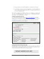
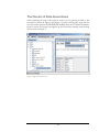
Figure 1 shows the ProteoLens interface. You can navigate both database and filebased input choices from the filesystems window as will be described in subsequent
sections. For visualization, a new network window can be opened in the right of the
interface through use of the Window menu accessed from the top menu bar of the
interface.
Figure 1. ProteoLens interface. This is what a user sees when first launching the ProteoLens application.
Example Data: Diseases and their Genes
The ProteoLens application comes with various example data sets. In this tutorial
guide, the file gene_disease.txt is a two-column tab-separated flat file containing
content structured in the manner below (based on data from Goh et al. 2007):
DISEASE_NAME
GENE_SYMBOL
Bladder_cancer FGFR3
Bladder_cancer KRAS
Bladder_cancer RB1
Bladder_cancer HRAS
Breast_cancer CHEK2
Breast_cancer PIK3CA
.
.
.
.
.
.
Pancreatic_cancer
RBBP8
Renal_cell_carcinoma FLCN
Renal_cell_carcinoma RNF139
Renal_cell_carcinoma OGG1
Renal_cell_carcinoma PRCC
Renal_cell_carcinoma TFE3
Renal_cell_carcinoma MET
Renal_cell_carcinoma VHL
Stomach_cancer KRAS
2
Optional: Installing and Configuring Oracle XE
A principal advantage of ProteoLens is how it directly connects with a database. To
help you get started, brief instructions are provided here for downloading and installing
Oracle XE, a free, basic entry-level database. This optional step of installing Oracle XE
is a task separate from, but strongly complementary to, the 10-minute tour in this
guide.
Oracle XE can be downloaded from:
http://www.oracle.com/technology/products/database/xe/index.html
You will want to install from the OracleXE.exe or the OracleXEUniv.exe file.
You will need to specify three parameters during the installation. The values used for
the examples in this manual are indicated.
1) Destination Folder: C:\oraclexe
2) HTTP Listener Port: 8081
3) System administrator password (for both SYS and SYSTEM): your choice
Note, the database SID (db_name) for OracleXE is set to “XE” by default.
Viewing the database
A default installation of Oracle XE places the application, Oracle Database 10g
Express Edition, in your main start menu list of programs. Selecting the Oracle
Database menu item provides you with a link: “Go to Database Home Page.” The web
interface to Oracle XE is a simple-to-use interface providing a range of options from
administration (including the creation and management of non-administrative users),
browsing of database objects (such as tables and views), creation and launching of SQL
scripts, and utilities that include options for loading external data into the database
system.
During installation, configuration, and uploading of content, it is important to make
note of five basic parameters:
1) the database user that has permissions to the content you wish to access from
ProteoLens – after installation, you may ideally wish to create a nonadministrative level user Oracle XE account for connecting to ProteoLens
application (you will need to remember the password associated with this
account);
2) the SID containing content you wish to connect to – by default this is set to
“XE”;
3) the table name with content you wish to access and query from ProteoLens;
3
4) the port number to the Oracle XE application – default value is 1521; and
5) the IP address hosting the Oracle XE application – this will probably be
127.0.0.1 unless you are installing Oracle XE on a computer separate from the
one you are using ProteoLens.
This manual presumes the following values for connecting to Oracle XE:
user name = MYTESTUSER; SID = XE; table name = GENEDISEASETABLE;
port number = 1521; and IP address = 127.0.0.1.
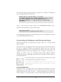
Creating a non-administration level user
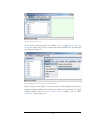
Go to the database web interface page (e.g., http://127.0.0.1:8081/apex) and, after
logging in with the SYSTEM user, use the Administration link and select the Database
UsersCreate User option. You may then create a non-administration level user
from the provided interface as shown in Figure 2.
Figure 2. Creating a non-administration level user for Oracle XE.
Uploading File-based Data with SQL*Loader (sqlldr)
You first need to create the table structure you want to load data into. Login as
MYTESTUSER and, through the SQL link on the Oracle XE web application, open
an SQL command window and enter the following command:
CREATE TABLE "GENEDISEASETABLE"
("DISEASE_NAME" VARCHAR2(100) NOT NULL ENABLE,
"GENE_SYMBOL" VARCHAR2(100) NOT NULL ENABLE)
4
The following file, gene_disease_load.ctl, is provided as an example of loading data
from a tab-separated file into Oracle XE:
OPTIONS (SKIP=1) LOAD DATA INFILE 'C:\Program
Files\IUPUI\ProteoLens_1.1.1\examples\gene_disease.txt' REPLACE
INTO TABLE GENEDISEASETABLE FIELDS TERMINATED BY x'09'
OPTIONALLY ENCLOSED BY '"' TRAILING NULLCOLS (DISEASE_NAME,
GENE_SYMBOL)
After you have created the table structure for GENEDISEASETABLE, open a
Windows command prompt, and type the following:
sqlldr control=C:\Program
Files\IUPUI\ProteoLens_1.1.1\examples\gene_disease_load.ctl
After entering this command, you will be prompted to enter the appropriate username
(e.g., MYTESTUSER) and password.
Connecting to Database and File-based Input
When using ProteoLens, the general form of input is either a two or three-column
relational format.
In the ProteoLens user application, this form of input can be accessed from either a
flat file or a supported database type. Supported database types are Oracle and
PostgreSQL. Databases can be accessed across the network or hosted on the same
computer running the ProteoLens application. The advantage of connecting to a
database for input is that you can quickly iterate through different relational
associations based on sending SQL queries from the ProteoLens interface directly to
the backend database.

A connection begins with using the Filesystems window and viewing
a file or database object (right-click with mouse).
It is at this point of the manual that the 10-minute exercise begins. This exercise
assumes that you have installed Oracle XE on your system with a user named
MYTESTUSER.
Connecting to Database Input
In order to connect to a database object, you must first mount the database. To mount
the database, you need to right-click on the root Filesystems node in the Filesystems
window and select the Mount database… option that appears in the submenu as
shown in Figure 3. As shown in Figure 4, use the Thin connection type and enter the
5
parameters as described in the previous section in this manual on installing and
configuring Oracle XE.
Figure 3. Right-clicking on the root-level Filesystem node presents the Mount Database option.
Figure 4. Specifying connection parameters for mounting a database. The settings shown are based on a default installation of Oracle
XE and the existence of a username MYTESTUSER.
6
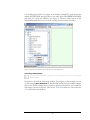
Use the Filesystem window to navigate to the database (named XE), open the schema
named MYTESTUSER and right-click on the table object GENEDISEASETABLE
and select View from the submenu (see Figure 5). The next major section of this
manual will describe how you convert the resulting view into a data association.
Figure 5. Using the ProteoLens interface to select a table object from an OracleXE database.
Connecting to File-based Input
You may choose to skip this step since the rest of the tutorial exercise relies on the database
input connection.
Navigate to a file with the Filesystems window. For purposes of this example, you can
use the example gene_disease.txt file bundled with the ProteoLens installation. Rightclick on the file that contains data you wish to input into ProteoLens, and a submenu
will emerge as shown in Figure 6. Click on the Table data check box. Then select the
View option from the submenu.
7
Figure 6. Using a Filesystems submenu to view the table data of a file.
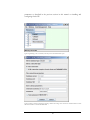
A window then appears as shown in Figure 7 and appropriate options are selected. For
this exercise, you should select Tab for the field separator and click on the checkbox
for the first row containing column names.
Figure 7. Previewing flat file data for import into the ProteoLens application.
After you have completed the View action on your input file, the next step would be
to create a data association as described in the next section.
8
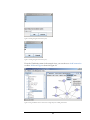
The Fine Art of Data Associations
After completing the steps in the previous section, you can proceed to make a data
association as shown in Figure 8 and Figure 9. For this tutorial guide, work with the
view that comes from the GENEDISEASETABLE object in the OracleXE database.
Figure 8 shows the window that appears in the ProteoLens interface after selecting
View as shown in Figure 5.
Figure 8. Creating a data association (part 1).
9
Figure 9. Creating a data association (part 2).
A special note about data associations
Data associations in ProteoLens are the architectural layer that wraps external data
from flat files or database tables in a uniform way. Importantly, as described in the user
manual:
The [ProteoLens] application makes no domain-specific assumptions about the
nature and meaning of the provided data, which leaves the user with responsibility of
using right data at the right place, but also allows for very high flexibility.
As will be described in the next section, data associations can be used for either
visualization or annotation.
Viewing and Annotating a Network
Visualizations and annotations are created from data associations. A visualization is the
graphical layout of nodes and edges in the network. An annotation is the modification
of nodes (e.g., labels, sizes, colors) or edges (e.g., labels, line widths, colors) based on
input that links to the identities of the nodes or edges.
Visualization - Showing the Network
Visualization starts with opening a network view through the Window menu as shown
in Figure 10.
10
Figure 10. Opening a new network view.
In the newly opened Network View window, the LoadNetwork from data
association option can be used to construct the network based on the uploaded data
association (see Figure 11).
Figure 11. Beginning the process of loading a network from a data association.
Figure 12, Figure 13 and Figure 14 show the process of selecting the network source,
specifying loading conditions and receiving the output view respectively. To specify
loading conditions from the Select network source interface, click on either
Condition… button (Figure 12).
11
Figure 12. Select network source interface. From this interface, you will need to specify loading conditions using the Condition
buttons, prior to clicking on the OK button.
Figure 13. Interface for specifying loading conditions. A basic set of steps for using this interface is: 1) select genedisease from the list
of available data associations (upper left); 2) highlight all values that appear in the data values window (lower right); and 3) click the OK
button. Upon returning to the „Select network source” interface shown in Figure 12, click the OK button there also.
After completing the steps of selecting the network source and specifying loading
conditions, a network view will appear similar to the network shown on the front cover
of this instruction manual. Note however that, as you repeat the exact same procedure,
the node-to-node associations will remain the same, but the physical layout of the
network on the screen will be somewhat random. The network shown presents how
genes link to each other through association with the same disease.
To construct a network that connects diseases directly together based on having a
common gene, you can substitute with the following SQL when viewing the
12
GENEDISEASETABLE object (Figure 5), create a data association, and repeat the
steps in Figure 12, Figure 13 and Figure 14:
SELECT A.DISEASE_NAME AA, B.DISEASE_NAME BB from
MYTESTUSER.GENEDISEASETABLE
a,MYTESTUSER.GENEDISEASETABLE b
where a.GENE_SYMBOL=B.GENE_SYMBOL and
A.DISEASE_NAME!=B.DISEASE_NAME
group by A.DISEASE_NAME, B.DISEASE_NAME
The resulting network view based on the substituted SQL is shown in Figure 14.
Figure 14. Output view of disease-to-disease associations shown only with defaults for node and edge annotations.
13
Annotating the Network
Annotating the network also utilizes data associations. For annotating nodes, the
specified data association takes the form of an ordered pair: {node_name,
annotation_value}. For annotating edges, the specified data association takes the form
of an ordered triplet (where node1 and node2 indicate the edge): {node1_name,
node2_name, annotation_value}.
With SQL, you can build these annotation tables from your original annotation table
(without uploading new tables into your database environment). Follow the steps
described in Figure 8 and Figure 9, and use the SQL commands below to define data
associations: diseasecount and edgecount.
SQL command for diseasecount:
SELECT DISEASE_NAME, count(GENE_SYMBOL) m
FROM MYTESTUSER.GENEDISEASETABLE
GROUP BY DISEASE_NAME
For annotating edges, a 3-column table is specified, typically with SQL. Typical usage is
to have the first two columns specify the identity of each edge, and the third value
(third column) is the annotation for that edge. Here is an example of building an
annotation table for edges with SQL as shown in Figure 15, Figure 16 and Figure 17.
SQL command for edgecount:
SELECT A.DISEASE_NAME AA, B.DISEASE_NAME BB,
count(B.DISEASE_NAME) M from MYTESTUSER.GENEDISEASETABLE
a,MYTESTUSER.GENEDISEASETABLE b
where a.GENE_SYMBOL=B.GENE_SYMBOL and
A.DISEASE_NAME!=B.DISEASE_NAME
group by A.DISEASE_NAME, B.DISEASE_NAME
Figure 15. Creating the edgecount annotation (part 1).
14
Figure 16. Creating the edgecount annotation (part 2).
Figure 17. Creating the edgecount annotation (part 3).
From the Visualization menu in the network view, you can choose to Add annotation
to either Nodes or Edges as shown in Figure 18.
Figure 18. Using Visualization menu of a network view to begin the process of adding an annotation.
15
Figure 19 and Figure 20 show the specification of a new node annotation and a new
edge annotation.
Figure 19. Specifiying a new node annotation with the diseasecount data association.
Figure 20. Specifying a new edge annotation with the edgecount annotation.
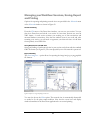
The resulting, annotated disease-to-disease network is shown in Figure 21.
16
Figure 21. Final output view of annotated nodes and edges of a disease-to-disease network. The thicker lines represent a greater
number of genes in common between the corresponding pair of diseases. The enlarged nodes represent those diseases that occur most
often in the disease-to-disease association.
From Figure 21, we observe that the colon cancer and leukemia have the highest
numbers of listed genes, and that stomach cancer and mesothelioma have the lowest
numbers of listed genes.
We can also infer that ovarian cancer has a greater percentage of its listed genes in
common with colon cancer than the percentage of listed colon cancer genes that are in
common with ovarian cancer.
17
Managing your Workflow: Sessions, Saving, Export
and Printing
Options for exporting and printing network views are provided in the Network menu
of the Network window as shown in Figure 22.
Sessions and Saving
From the File menu of the ProteoLens interface, you can save your session. You can
then close ProteoLens and reload your session at a later time. Sessions are saved in
XML format. A saved session contains your working set of data associations and
mounted database connections. Note that the window layout is not saved and, after
restarting your session, you will need to regenerate your network views or load them
from separately saved GML files.
Saving Network Files with GML Files
Saving and loading of each network view in your session can be done with the standard
GML file format (see Figure 22). The exact physical layout of the network is preserved.
Export and Printing
The Save image as… option allows for exporting the image into jpeg or png graphical
file formats.
Figure 22. Options for saving and printing network views.
You can also choose the Print option. The network view is automatically downscaled
as needed to fit the print output medium. Note that the zoom level and display
window boundaries in the ProteoLens application do not control printing.
18
Important Notes on Usage
At the time of this writing, to ensure the highest amount of compatibility between
database and java resources, we make the following recommendations for character
sets used in table names, column names, and data field values:

Use capital characters and underscores for table names and column names.

Do not use spaces inside data field values (instead of “Retinal cell carcinoma”,
use “Retinal_cell_carcinoma”).

Be aware of the 30 character length limitation on table names and column
names in Oracle XE.

In order to avoid appending spaces to data field values, use VARCHAR2 as a
column type and not CHAR.
The example data files in the ProteoLens installation and the contents of this guide are
consistent with the above recommendations.
19