Download User manual - Latent variable models handled with optimization

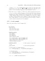
10
CHAPTER 2. THE LANGUAGE AND THE PROGRAM
declaring xi to be of type random effects vector. But, more important is that
random effects can be used also in non-Gaussian (nonlinear) models where we are
unable to derive an analytical expression for the distribution of (X, Y ).
5. Why didn’t we try to estimate σe ? Well, let us count the parameters in the model:
a, b, µ, σ, σx and σe ; totally six parameters. We know that the bivariate Gaussian
distribution has only five parameters (two means and three free parameters in the
covariate matrix). Thus, our model is not identifiable if we also try to estimate
σe . Instead, we pretend that we have estimated σe from some external data source.
This, example illustrates a general point in random effects modelling: you must be
careful to make sure that the model is identifiable!
2.2.1
A code example
Here is the random effects version of simple.tpl:
DATA_SECTION
init_int nobs
init_vector Y(1,nobs)
init_vector X(1,nobs)
PARAMETER_SECTION
init_number a
init_number b
init_number mu
vector pred_Y(1,nobs)
init_bounded_number sigma_Y(0.000001,10)
init_bounded_number sigma_x(0.000001,10)
random_effects_vector x(1,nobs)
objective_function_value f
PROCEDURE_SECTION
f = 0;
pred_Y=a*x+b;
// This section is pure C++
// Vectorized operations
// Prior part for random effects x
f += -nobs*log(sigma_x) - 0.5*norm2((x-mu)/sigma_x);
// Likelihood part
f += -nobs*log(sigma_Y) - 0.5*norm2((pred_Y-Y)/sigma_Y);
f += -0.5*norm2((X-x)/0.5);
f *= -1;
// ADMB does minimization!