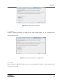
1
CrysAlisPro Data Collection and Processing Software for Agilent X-ray Diffractometers User Manual Read the main diffractometer user manual, in particular the Health and Safety information, before operating CrysAlisPro with the diffractometer. Revision 5.2, January 2013 Agilent Technologies, XRD Products 10 Mead Road, Yarnton, Oxfordshire. OX5 1QU, UK Tel: Fax: +44 (0)1865 291600 +44 (0)1865 291601 http://www.agilent.com/chem DOCUMENT REVISION LOG Document revision log Revision Date Person(s) responsible Approval Reason for update 5.2 18/01/13 Daniel Baker Adrian Jones Update of new features from software release 171.36.24 CrysAlisPro USER MANUAL Contents 1 Introduction.......................................................................................................................................................... 1 1.1 Contacts List............................................................................................................................................... 1 2 Installation ........................................................................................................................................................... 2 2.1 2.1.1 3 Open CrysAlisPro ......................................................................................................................................... 2 Select experiment ................................................................................................................................. 3 2.2 Close CrysAlisPro......................................................................................................................................... 4 2.3 2.4 GUI interface guide.................................................................................................................................... 4 Software updates....................................................................................................................................... 5 Hardware Control ................................................................................................................................................ 6 3.1 Device Control ............................................................................................................................................ 6 3.1.1 Shutter Closed/Open ........................................................................................................................... 6 4 3.1.2 X-ray Mo/Cu .......................................................................................................................................... 6 3.1.3 CCD .......................................................................................................................................................... 6 3.1.4 Cryo.......................................................................................................................................................... 6 3.1.5 Xray.......................................................................................................................................................... 6 3.1.6 Level ........................................................................................................................................................ 8 3.1.7 IO .............................................................................................................................................................. 8 3.2 3.3 Status Display ............................................................................................................................................ 8 Command (CMD) Shell: ............................................................................................................................ 8 3.4 Service ....................................................................................................................................................... 10 Standard small molecule experiment ............................................................................................................ 12 4.1 Screening .................................................................................................................................................. 12 4.1.1 CellCheckCSD ...................................................................................................................................... 14 4.1.2 Local database..................................................................................................................................... 15 4.2 4.3 Pre-experiment ......................................................................................................................................... 15 Strategy calculation................................................................................................................................. 16 4.4 4.5 Data collection ......................................................................................................................................... 17 Data reduction .......................................................................................................................................... 18 4.5.1 Automatic data processing ............................................................................................................... 18 4.5.2 Data reduction with options .............................................................................................................. 19 4.6 Structure solution .................................................................................................................................... 20 4.6.1 AutoChem2.0 ......................................................................................................................................... 20 CONTENTS 5 6 4.6.2 WinGX launcher .................................................................................................................................. 20 4.6.3 Olex2 launcher...................................................................................................................................... 20 4.6.4 Crystals launcher................................................................................................................................. 21 4.6.5 Jana launcher ...................................................................................................................................... 21 Data collection for protein crystallography .................................................................................................. 22 5.1 5.2 Data collection: screening...................................................................................................................... 22 Data collection: Full experiment............................................................................................................ 24 5.3 Data reduction .......................................................................................................................................... 24 5.4 5.5 Exporting files........................................................................................................................................... 24 Advanced data collection modes .......................................................................................................... 24 Other data collections ...................................................................................................................................... 26 6.1 Special/Append data collection............................................................................................................ 26 6.2 Powder diffraction ................................................................................................................................... 26 6.2.1 Powder experiment ............................................................................................................................. 26 6.2.2 6.3 Powder pattern creation .................................................................................................................... 27 Variable temperature/wavelength experiments ................................................................................ 27 6.4 Single image ............................................................................................................................................. 28 7 Lattice Wizard.................................................................................................................................................... 30 7.1 7.2 7.3 8 Peak hunting............................................................................................................................................. 30 Unit cell finding ........................................................................................................................................ 31 EwaldPro ..................................................................................................................................................... 31 7.3.1 Tool Bar ................................................................................................................................................ 31 7.3.2 Lattice viewer window ....................................................................................................................... 32 7.3.3 Crystal tab ............................................................................................................................................ 32 7.3.4 Filters Tab ............................................................................................................................................. 33 7.3.5 Selection Tab ....................................................................................................................................... 34 7.3.6 Groups ................................................................................................................................................... 35 7.4 7.5 7.6 Refine instrument model ........................................................................................................................ 36 Lattice transformation ............................................................................................................................ 36 Twinning / multi-crystals ....................................................................................................................... 36 7.7 7.8 Incommensurates / Quasi-crystals ...................................................................................................... 37 Precession photo reconstruction .......................................................................................................... 37 7.9 Log window .............................................................................................................................................. 38 Inspection and Manipulation of Data ............................................................................................................ 39 8.1 Refinalization ............................................................................................................................................ 39 8.2 Twin data finalization .............................................................................................................................. 41 CrysAlisPro USER MANUAL CONTENTS 9 8.3 Running GRAL in interactive mode ...................................................................................................... 42 8.4 8.5 Filtering data ............................................................................................................................................. 43 Crystal shape modelling (face indexing).............................................................................................. 43 Appendix............................................................................................................................................................. 45 9.1 Layout and controls ................................................................................................................................. 45 9.1.1 Image list .............................................................................................................................................. 45 9.1.2 Predictions ........................................................................................................................................... 45 9.1.3 Pixel/area information ....................................................................................................................... 46 9.1.4 Header information/K (goniometer angles) ................................................................................... 46 9.1.5 Find hkl.................................................................................................................................................. 46 9.1.6 Look up table ....................................................................................................................................... 47 9.1.7 Colour table .......................................................................................................................................... 47 9.1.8 Zoom in ................................................................................................................................................. 47 9.1.9 Zoom out............................................................................................................................................... 47 9.1.10 Zoom localiser ................................................................................................................................. 47 9.1.11 Resolution rings .............................................................................................................................. 47 9.1.12 2D Peak profile ................................................................................................................................ 48 9.1.13 3D Peak profile (Rocking Curve) .................................................................................................. 48 9.1.14 Help ................................................................................................................................................... 48 9.1.15 View .................................................................................................................................................. 48 9.2 9.3 Key to power tool icons .......................................................................................................................... 49 External detector frame formats ........................................................................................................... 49 9.3.1 Dectris ................................................................................................................................................... 49 9.3.2 Rigaku ................................................................................................................................................... 50 9.3.3 SAXI ....................................................................................................................................................... 50 9.3.4 MAR....................................................................................................................................................... 51 9.4 File structure............................................................................................................................................. 51 9.4.1 Directory file structure ....................................................................................................................... 51 9.4.2 Experiment file structure ................................................................................................................... 52 9.5 9.6 CellCheckCSD installation ...................................................................................................................... 53 AutoChem2.0 installation ......................................................................................................................... 53 CrysAlisPro USER MANUAL CONTENTS FIGURES Figure 1: The experiment list window ...................................................................................................................... 3 Figure 2: Main window of CrysAlisPro software. Note that some icons are greyed out (inactive) during data collection, and can only be accessed in the offline mode of the software. ............................................. 4 Figure 3: Device control for the Xcalibur/Gemini system (left) and the Supernova system (right) .............. 6 Figure 4: Example of SuperNova device control window ...................................................................................... 7 Figure 5: Status display ............................................................................................................................................... 8 Figure 6: Command shell window ............................................................................................................................. 9 Figure 7: CCD options window................................................................................................................................... 9 Figure 8: Full calibration experiment window ....................................................................................................... 11 Figure 9: Pre-experiment screening window for small-molecule experiment ................................................. 12 Figure 10: Full screening window with strategy options highlighted ............................................................... 13 Figure 11: Check CSD window ................................................................................................................................. 14 Figure 12: Experiment strategy window, with each information section labelled .......................................... 16 Figure 13: Crystal screening window for PX experiment .................................................................................... 22 Figure 14: Crystal screening tab .............................................................................................................................. 23 Figure 15: Multi-temperature/wavelength experiment window ........................................................................ 27 Figure 16: Window showing temperature list for multi-temperature/wavelength experiment ................... 28 Figure 17: Main lattice wizard window .................................................................................................................. 30 Figure 18: Ewald Explorer tool bar (part 1) ............................................................................................................ 31 Figure 19: Ewald Explorer tool bar (part 2) ............................................................................................................ 32 Figure 20: Crystal tab in EwaldPro ............................................................................................................................ 32 Figure 21: Filters tab in the Ewald Explorer ........................................................................................................... 34 Figure 22: Selection/Lattice-lt tab in Ewald Explorer .......................................................................................... 34 Figure 23: Example of Lattice-lt function in Ewald Explorer ............................................................................... 35 Figure 24: Groups window in Ewald Explorer........................................................................................................ 36 Figure 25: Data reduction finalizing window ......................................................................................................... 40 Figure 26: Twin data finalisation window .............................................................................................................. 41 Figure 27: Abs display window showing crystal image and face-indexing details......................................... 44 Figure 28: Run list generator for Dectris ................................................................................................................ 50 Figure 29: Run list generator for d*trek image format ......................................................................................... 50 Figure 30: Run list generator for SAXI .................................................................................................................... 51 Figure 31: Run list generator for MAR.................................................................................................................... 51 Tables Table 1: Control buttons in CrysAlisPro ................................................................................................................... 45 Table 2: Power tool icons ......................................................................................................................................... 49 CrysAlisPro USER MANUAL INTRODUCTION 1 Introduction CrysAlisPro has been designed to provide a user friendly, simple to use, graphical user interface for data collection and data reduction of single crystal X-ray diffraction data. Based on the CrysAlis CCD and RED programs the CrysAlisPro software provides greatly increased automatic functionality. CrysAlisPro provides direct visual access to data collection and reduction as well as other functions, all of which, in a single multi-threaded program, can be performed in parallel. This manual is designed to be a brief introduction to CrysAlisPro and its features. For more, in-depth information the „on-line help,‟ which is embedded into the CrysAlisPro software or the XRD forum (www.agilentxrdforum.com) should be consulted. The use of CrysAlisPro is limited to owners/users of Agilent Technologies/Oxford Diffraction equipment and their collaborators. If you are interested in using CrysAlisPro but are not an existing Agilent equipment user, please contact [email protected]. 1.1 Contacts List CrysAlisPro users are greatly encouraged to report any software bugs by sending details to [email protected]. Only by receiving bug reports from experienced users can these be successfully identified and repaired. Ideas for software improvement are also very much welcomed, and all are considered when creating new features for future editions of CrysAlis Pro. For specific crystallographic enquiries, use the [email protected] e-mail address and for general queries, try the forum www.agilentxrdforum.com. Hardware support: [email protected] Software support: [email protected] Crystallographic queries: [email protected] General information and resources: www.agilentxrdforum.com CrysAlisPro USER MANUAL 1 INSTALLATION 2 Installation To install CrysAlisPro you will first need to obtain a copy of the CrysAlisPro executable file and the 'Corrections' folder from your diffractometer PC. The executable comes in the following form: CrysAlisPro171_XX_YY.exe where XX = current version number and YY = the current release number. Step 1. Double click on the CrysAlisPro171_XX_YY.exe program. Follow the on screen instructions. Step 2. When asked to select the program elements required for installation click on the box next to PRO and HELP only (a tick appears in the box) and click on Next. Step 3. Once installation is complete double click on the CrysAlisPro icon which has been installed on the desktop. Step 4. If this is first installation of CrysAlisPro on your computer the user has to choose between two scenarios of first use: There will be a message box saying 'Choose start-up mode' - 'Do you want to set this application for Data Collection?' Yes: The computer is a data collection machine connected to Oxford Diffraction/Agilent Technologies hardware. This will open the "CrysAlisPro setup par file" generator. The dialog will guide you through a multi-step procedure to collect all system relevant information. It will require you to have the media with all correction files ready. No: Your computer is intended for data reduction only, you will need to have an Oxford Diffraction/Agilent Technologies data set situated on your machine (in the absence of data, locate the file ideal_small.zip from within the help folder of this installation - this will contain a dummy experiment allowing you to start). The program will present a message box 'Red fatal system start-up' asking you locate the *.par file of the aforementioned experiment. Click on Yes and locate the par file. 2.1 Open CrysAlisPro To start CrysAlisPro either double click on the icon on the windows desktop or navigate to Start -> All Programs-> Xcalibur (Agilent Technologies) -> CrysAlisPro (for Windows XP/7). Please note that there are two icons on your desktop for CrysAlisPro; one 'online' and one 'offline' (data reduction only). When the program is started on a PC connected to an Oxford Diffraction/Agilent Technologies diffractometer, CrysAlisPro will start-up in 'online' mode. This means the program will connect to the diffractometer, CCD and other devices. On start-up, the software initialises the hardware. Commands cannot be accepted until all hardware initialisation procedures are complete. Wait until the CCD status is shown as Ready before issuing commands. The windows header carries the text 'online'. CrysAlisPro USER MANUAL 2 INSTALLATION When a second version of CrysAlisPro is started or, if CrysAlisPro is opened on a standalone PC, this 'offline' version will open in data reduction mode only (without control of the devices and diffractometer control) and will ask the user to select the 'experiment' that they want to work on from the experiment database. 2.1.1 Select experiment Opening CrysAlisPro in the offline mode opens a window which allows browsing within a list of experiments (Figure 1). Figure 1: The experiment list window The list may be refined by using the tick boxes for Hide pre-experiments and Hide screenings. The lists may be defined for an individual or over a set time period: using the >> button in Name of list will open a window which will allow parameters to be selected so only certain experiments appear in the defined list. These lists may be deleted or removed. More experiments may be added to the list by selecting the Multiple addition option or an individual experiment may be found by clicking Browse experiment. The displayed information may be changed to one of the pre-set views (choose between Standard, or Volume, laue, wavelength, Rint, redundancy or Protein screening) or Custom columns may be set. CrysAlisPro USER MANUAL 3 INSTALLATION 2.2 Close CrysAlisPro To close CrysAlisPro, click on the X icon in the top right corner of the CrysAlisPro screen. When in CCD mode, a prompt will appear regarding generator ramping control. For micro-focus systems in particular, it is recommended that users ramp the generator down when the diffractometer is not in use. This will leave the generator running in stand-by mode with minimal power settings to help extend the lifespan of the X-ray tube. For all other systems it is up to the users individual preferences as to the power settings used when the system is not in use. 2.3 GUI interface guide Figure 2 highlights the features of the main software window. These are covered in greater detail throughout this document. D A B E C F Figure 2: Main window of CrysAlisPro software. Note that some icons are greyed out (inactive) during data collection, and can only be accessed in the offline mode of the software. The main features include: A. Power tools: access to the lattice wizard, command shell, refinalisation features, as well as links to structure solution software (for full list of icons see Section 9.2). CrysAlisPro USER MANUAL 4 INSTALLATION B. Main window: shows current frame in online mode, and selected frame or precession unwarp image in offline mode. C. Layout and controls: allows user to scroll through frames, get peak information, change brightness, and use peak profile tools (for full list of features see Section 9.1). D. Device control: Only shown in the online mode of the software, and shows status of shutter, which source is in use, and provides access to CCD/cryo device/X-ray tube information. E. Information tabs: Provide information about the current unit cell, data collection progress, and a summary of the data reduction. Additional features can be accessed via the > buttons. F. SM/PX button: allows the user to switch the software between small molecule and protein modes. 2.4 Software updates CrysAlisPro is continually updated with new features and bug fixes. Beta-test versions of the software are in constant use by Agilent Technologies employees, and the most stable of these is released for customer use approximately every six months. Releases can be downloaded from the XRD forum. Each new edition of CrysAlisPro is released with details of bug fixes and additions since the previous issue. This information can be found in the Help menus under Reference section/Version news. It is possible to install a new version of CrysAlisPro without having to uninstall the previous release. If required, older versions may be uninstalled using the standard windows „remove programs‟ procedure. CrysAlisPro USER MANUAL 5 HARDWARE CONTROL 3 Hardware Control 3.1 Device Control The Device control is only available when CrysAlisPro is in online mode. In offline mode, only the status area is shown. Figure 3: Device control for the Xcalibur/Gemini system (left) and the Supernova system (right) 3.1.1 Shutter Closed/Open This icon indicates the current status of the X-ray shutter; this can either be Open (red) meaning the sample is exposed to X-rays or Closed (green) meaning the sample is not exposed to X-rays. 3.1.2 X-ray Mo/Cu This button is only visible on a dual wavelength system. The source is automatically selected (according to the machine defaults) upon system start-up. Clicking on this button switches between sources. Selecting Yes on the pop up window will switch wavelength and force ramping up of the generator to the standard data collection power; selecting No will switch wavelength but keep the generator at the standby values; selecting Cancel will stop any wavelength changing. 3.1.3 CCD This opens the software device controller for the CCD head. The display will show the running temperature of the CCD and the % power being used to maintain this temperature. 3.1.4 Cryo Clicking this icon will open the device controller window for cryodevices (if there is one installed). Right clicking this icon allows the appropriate cryodevice to be selected. Devices supported include: Cobra, Cryojet, Cryostream (600 and 700), Helijet and Hotjet. Within this menu it is possible to display the current sample temperature in the image window by selecting Display current sample temp. 3.1.5 Xray Clicking the X-ray generator controller icon opens a window to display and control generator settings. The Read Values box displays the actual Voltage (kV), Current (mA), Power (kW) and Temperature (°C) of the system. The Set values box displays the target power of the source and its on/off status. CrysAlisPro USER MANUAL 6 HARDWARE CONTROL Figure 4: Example of SuperNova device control window The Emergency X-RAY OFF button quickly shuts the generator down and stops the production of X-rays in an emergency. After such an event, the hardware interface needs to be reinitialised (switched off and on) before setting the next Voltage and Current. In dual source systems, the Second lamp button displays the status of the non-active source. The Start/Stop button initiates or ends communication between the software interface and the generator. Use the Set kV and mA X-ray button to alter the power of the tubes. Typical settings for both Molybdenum and Copper fine-focus tubes (Xcalibur and Gemini systems) are 50 kV and 40 mA (although some users prefer 40kV and 40mA for Copper). For Micro-focus systems (Mova and Nova), standard generator settings are 50kV and 0.8mA. The generator will reach the desired values in a stepwise and controlled manner. NOTE: If you close the window before the ramp process is complete then only the values at closure will be reached. The Fault and Status indicators provide feedback for the state of the generator. In normal operation only the Status indicators should be active. The Fault indicators can be used as guides for investigating hardware issues should there be any trouble with the generator. A log file for the generator output is automatically recorded from the beginning of the experiment and this can be viewed at any time by clicking the Plot button. For automatic generator ramping control go to CMD > CCD options and click on the Generator tab (see section 3.3). CrysAlisPro USER MANUAL 7 HARDWARE CONTROL 3.1.6 Level The liquid nitrogen level controller icon brings up a window panel indicating the level of liquid nitrogen in the tank (if there is an autofill connection). The level is expressed as a percentage, with 100% indicating that the tank is full. 3.1.7 IO This IO device control button brings up a window with access to software control of the cabinet lights, and resetting of the emergency stop button. 3.2 Status Display The status display, located underneath the device control, provides information on the activity of the instrument and software processing (see Figure 5). Figure 5: Status display CCD status: gives feedback of the current status of the data collection CCD thread (only in online mode) RED status: gives feedback of the current status of the data reduction RED thread. Progress bar: shows the progress of the current process, for example, the percentage completeness of the pre-experiment or data collection. 3.3 Command (CMD) Shell: This button on the left-hand side of the main screen opens a history window with an attached command line. CrysAlisPro may be run „automatically‟ through the GUI (menus and buttons) or „manually‟ using commands entered into this command line. The user can access all existing (and historical) functions using “manual” commands. Either the entire experiment may be run completely in this mode or the window may be opened simply to issue specific commands. A list of commands and their functions are available in the online help (or type COMMAND HELP into the command line). The main part of the window contains a history terminal, which is always active (continuously updated) and can be referred to by the user for further information. This history window can be viewed in either CCD or RED modes and it is possible to toggle between these using the tabs at the top of the window. (The CCD tab is only available when CrysAlisPro is in the „online‟ mode). When issuing commands, it is important that the correct mode is chosen. The command shell window can be opened or closed at any CrysAlisPro USER MANUAL 8 HARDWARE CONTROL time and can be resized. Close the command shell by clicking on the button located in the bottom right hand corner of the window. Figure 6: Command shell window Options CCD/RED: This button provides access to the machine and software setup. There are many tabs which control the functions of the hardware and software. It is not generally necessary to change any settings however, listed below are some usful options which may be employed. Figure 7: CCD options window CrysAlisPro USER MANUAL 9 HARDWARE CONTROL Fonts: use this tab to change the displayed font size in specific windows of CrysAlisPro. Beam stop: allows adjustment of the beamstop mask. Reflections that fall under the mask are rejected. This is set up during installation but can be adjusted here. Decreasing the size may help retrieve low angle reflections and can also improve the quailty of the extracted powder patterns. Goniometer: allows acivation of de-icing runs at the end or during data collections. This is useful when using a low temperature device coulped with long exposure times. Generator: here it is possible to set the time for automated generator ramping. This will help preserve the tube life by lowering the voltage and current settings to stand-by values after a period of non-use. Programs: direct CrysAlisPro to the location of your favourite structure solution program. E-mail: set-up hardware, software and experiment status notifications, emailed directly from your system. e.g. low N2 level, generator trip, Laue group change, end of experiment. 3.4 Service This power tool collects those service commands most commonly accessed by the user into one defined area. It is recommended that they are only used under guidance from Agilent employees. These commands include: Shutter: to manually control the opening and closing of the shutter. CCD options: to reinitialise or reset the CCD, or remove the dark images. Goniometer: for direct goniometer control and home flag search*. Image control (CCD pars): to change any CCD parameters and record diffraction images. Configuration file paths: points the software to specific CCD setup file (.par file) and Correction files (.geo, .ffi,.ffinf and .ccd files). Instrument calibration: to start new or resume calibration experiments. This facility should not be needed other than during installation and service visits, but if persistent problems are encountered, the user may be advised to recalibrate the instrument. Align SuperNova optics: - should not be used unless the user has been appropriately trained. Tools: the „Make zip‟ is a useful feature for zipping up complete experiments into a single file for easier archiving or to send to the software team for problem resolution. *WARNING: It is advisable to contact a service engineer or e-mail [email protected] before attempting manual goniometer control, as no collision protection is provided in this mode. Calibration: Generally calibrations are run for three purposes: Instrument model calibration Instrument model calibration at specific detector distances (useful for powder experiments) CrysAlisPro USER MANUAL 10 HARDWARE CONTROL Instrument model calibration with additional flood calibration If required, an automated procedure is normally used, with data collected at two different detector distances (near and far) on a test crystal (an ylid test crystal is provided with the system). With dual wavelength systems, the procedure is carried out for both sources. In order to save time, calibration experiments are often run without frame correlation or overflow re-measurements, both of which can be switched on/off in the Calibration Experiments window. The experiment can be further optimised by changing the resolution and exposure times (Figure 8). The calibration can be monitored in the Command Window and an output message is generated upon finishing which details the instrument parameters, test crystal unit cell dimensions and the percentage fit for indexed reflections As the amount of data required for a system calibration is typically less than that required for a structure determination, an option is included to collect additional frames for those users who wish to refine structures from calibration data for system benchmarking. Figure 8: Full calibration experiment window CrysAlisPro USER MANUAL 11 STANDARD SMALL MOLECULE EXPERIMENT 4 Standard small molecule experiment This section explains the main features involved in performing a single-crystal diffraction experiment for small molecule samples, from the initial screening of samples, to analysing the data from the preexperiment, devising a suitable data collection strategy, and finally to the data collection, reduction and structure solution. Before beginning an experiment, it is useful to have some knowledge of the chemical composition of the sample, to select the appropriate system parameters, e.g. wavelength, temperature, detector distance. 4.1 Screening 1. Check that the appropriate X-ray source is selected (if using a dual source system) and that the generator settings are correct (see section 3.1.5). 2. Ensure the software is running in “small molecule” mode by checking that the CrysAlisPro icon on the bottom right of the screen has the suffix SM. If not then click on this icon and select small molecule mode in the SM/PX window. 3. Click on Start/Stop and select Start new experiment. The pre-experiment window will appear (see Figure 9). Figure 9: Pre-experiment screening window for small-molecule experiment 4. In the Path and user/Sample section input the sample name and path for storing the data files. If known, enter the Expected chemical formula (which is used for absorption corrections and assisting in structure-solution) and add a comment about the sample. The last used formula can be recalled with the Get Last used formula button. The user running the experiment can be set with CrysAlisPro USER MANUAL 12 STANDARD SMALL MOLECULE EXPERIMENT the Set user button, and additional details about the sample can be recorded using the Sample 5. description button. The user now has three options, to proceed to the Mount sample screen to align the crystal, to go straight on to Fast Screening of the sample (with setup options configurable from the >> button), or to setup the pre-experiment manually via the Configure Pre Manually button. The default choice for most users will be Mount sample. 6. Clicking on Mount sample opens up a new window which activates the video camera, and is used to align the crystal in the beam (more details can be found in Section 8.5). From that window the Exit & Screen button starts the screening experiment. 7. By default ten images of the sample will be recorded, which can be used to check sample quality, and determine the details of the pre-experiment (see Figure 10). If the crystal quality is too poor, the user can simply click on Mount sample again and repeat the process to quickly check through several candidate crystals. Information about crystal quality and suggested unit cell parameters is shown next to the accumulated diffraction image. Figure 10: Full screening window with strategy options highlighted 8. There are three details to consider when deciding whether a crystal is suitable for data collection: Peaks: The number of peaks that fit the proposed unit cell is shown. Unit Cell: Details of the point group and lattice parameters are given based on the screening data collection. The user has the option to access the CSD module at this time to compare the unit cell with other structures present in the database (see Section 4.1.1 for further details). Quality: Estimates of the I/sigma values are given out to various resolution values, and a guide is given as to how well the sample diffracts. The diffraction limit and mosaicity of the sample is also estimated. CrysAlisPro USER MANUAL 13 STANDARD SMALL MOLECULE EXPERIMENT 9. Details of the calculated pre-experiment are shown at the bottom of the screen, with the option for the user to define what strategy they would like to aim for with regards to the actual experiment (Figure 10). To override the suggested settings the slider allows for a manual adjustment of the exposure time, and the drop-down menu offers different types of experiments, such as complete, redundant, or time-limited collections. Select Start to begin the pre-experiment. 4.1.1 CellCheckCSD The Cambridge Structural Database (CSD) is a database containing many molecular crystal structures and is populated by structures submitted to the Cambridge Crystallographic Data Centre (CCDC). Developed in collaboration with the CCDC, CellCheckCSD is a freely available plug-in (via www.ccdc.cam.ac.uk) for CrysAlisPro. Every time a cell is found or updated, CellCheckCSD searches for „hits‟ or structures closely related in unit cell parameters to the found unit cell. The CSD link appears in various places in CrysAlisPro software and is a useful tool for spotting structures which are already in the public domain. It is particularly useful during the screening process to check that the crystal isn‟t an unwanted starting reagent. The number of hits is displayed within the link and clicking this link, opens a window as shown in Figure 11. Figure 11: Check CSD window The window may be re-sized to view the data more easily. The drop down menu allows various cells (current, constrained, average, and final) to be used as the search. Two buttons can be used to start or stop manual or automatic searching of the CSD and alongside these is an Options button. Clicking Options opens a window to allow the search parameters to be altered according to your requirements. The window displays the hits which are most closely matched to the cell and the most likely has the highest cell match % value. The formula, symmetry and Refcode are displayed but are not used as search parameters. Individual hits may be deselected using the tick boxes or the Select all and Deselect all buttons may be used CrysAlisPro USER MANUAL 14 STANDARD SMALL MOLECULE EXPERIMENT It is possible to view the selected hits, either in Mercury* (if you have a CSD license installed locally on the PC) by clicking View in Mercury or on the WebCSD (again a license is required) by clicking Go To WebCSD. *Mercury is a program distributed by the CCDC. Visit www.ccdc.cam.ac.uk for more information. 4.1.2 Local database It is also now possible to create your own local database of structures to search against when using the CellCheckCSD feature. To activate, simply click on the Options button in the Check CSD window, and tick Enable local database search. Clicking on the Create from lists button will search through all previous experiments that have been run on the PC and then add the results to the database. It is also possible to browse any folder containing .res/.ins/.cif files. Databases from other PCs can be merged using the Import xml button. Any previous experiment (or stored .res/.ins/.cif file) that matches the current unit cell settings will now appear in the drop-down list. Green entries are local experiments, and can be accessed by doubleclicking on them, which brings up a new offline instance of CrysAlisPro. A red entry indicates an experiment which is currently open in CrysAlisPro. Any local entries that are black indicate that the original experiment is not available. 4.2 Pre-experiment Before the main data collection a pre-experiment is run to better determine the unit cell parameters, diffraction symmetry and the other properties of the diffraction pattern required to calculate a suitable collection strategy. During the pre-experiment an information card will appear on the right-hand side of the screen displaying the user defined settings from the previous dialog and the unit cell of the crystal being measured. By default, 15 frames are recorded when using molybdenum, and 30 with copper radiation (15 low-angle and 15 high-angle). Once the first frame has been measured, the software will attempt to find the unit cell, crystal lattice, and evaluate the average I/sigma spread to a set resolution. This information will be updated after every frame. Using this information a suitable strategy will be calculated. The Start experiment button will become active, and the user can choose to start the main experiment using the information present in the preexperiment card. The default action is to wait for the completion of the pre-experiment and for the user to check the details of the experiment in the strategy window. If the Interactive strategy after pre box is not checked the software will automatically launch the full experiment. CrysAlisPro USER MANUAL 15 STANDARD SMALL MOLECULE EXPERIMENT 4.3 Strategy calculation On completion of the pre-experiment a strategy window opens automatically. Note that this can also be accessed directly by clicking on Start/Stop and selecting Start New (no pre-experiment) if no preexperiment is required. The window has several different components: A B D C G E F Figure 12: Experiment strategy window, with each information section labelled A. Unit cell for Strategy Calculation: contains the proposed unit cell, calculated from the preexperiment. The user has the option to analyse the pre-experiment data and change the unit cell by clicking on the Lattice Wizard button. Full details on the features within the Lattice Wizard can be found in Section 7. B. Strategy parameters: it is possible to set the maximum resolution of the data collection, choose how the strategy is collected (by Laue symmetry or by the sphere of reciprocal space) and set the detector distance. If the sample is suspected to be of chiral nature the Friedel mates box should be un-checked. The Advanced button allows for greater control over the experiment setup, and is discussed further in the online help. C. Strategy mode: includes options such as complete, redundant, and time-limited collections. Clicking on the IUCr limit button reduces the coverage to 98.5%, which is the minimum required for publication in an IUCr journal. CrysAlisPro USER MANUAL 16 STANDARD SMALL MOLECULE EXPERIMENT D. Time prediction: shows the predicted exposure times, based on the pre-experiment data and desired I/sigma value (usually set to 15 for good quality data). These values can be overridden by the user. The strategy can be optimized based either on achieving a relevant I/sigma level or time constraint. When collecting with copper radiation, it is usually necessary to collect for a longer time at higher angles (a ratio of 1:4 is recommended). If this is the case the user can select Different time for each theta position. It is also possible to change the scan width, which is useful for collecting weak reflections, or to help separate out close/overlapping peaks. E. Current Strategy: details the number of frames and length of the experiment. If any changes are made to sections A, B, C or D the user will need to click on the Calculate New Strategy button to update the experiment details. Advanced users may wish to create their own run list, which can be accessed via the Manually Edit Run List button the online help for more details). F. Coverage: graphs or tabulated views of the proposed data collection, showing the completeness and redundancy values for the chosen Laue group and for the full sphere of reciprocal space (P1). G. Settings/Options: there are three buttons in this section. The Data collection/Dark button lets the user change settings regarding correlation (prevents problems with zingers at long exposure) and dark current measurements. The CCD processing button allows the correction and binning mode of the CCD to be changed. The Autochem/Movie/Cryo/Red button lets the user choose to record a movie of the crystal, input the expected chemical formula, set AutoChem to attempt automatic structure solution (if the relevant license has been purchased). There is also a useful feature that will automatically shut down any hot/cryo device being used, once the experiment is finished. Click on Start Experiment to begin. By default, a „movie‟ is taken of the crystal for later reference or for face-indexing (see Section 8.5) and after reference dark images are recorded the experiment will start. 4.4 Data collection During the data collection it is possible to stop the experiment at any point by clicking on the Start/Stop button and selecting Stop All. The experiment can be resumed from this point at a later time, assuming the crystal has not been taken off the goniometer head, by clicking on Start/Stop and selecting Resume All. Whilst the experiment is running access is available to three information cards on the right-hand side of the screen: Crystal, Data Collection, and Data Reduction. A fourth card, named AutoChem, will appear if the relevant software has been installed and license purchased (see Section 9.6). The different cards can be maximized by clicking on the relevant card name. Additional options for the cards are found by clicking on either the card name when maximized or the > buttons. The Crystal card displays the current unit cell information, the sample chemical formula, Z value, and machine model parameters. Also displayed will be the Average unit cell from Proffit (CrysAlisPro‟s cell CrysAlisPro USER MANUAL 17 STANDARD SMALL MOLECULE EXPERIMENT refinement algorithm) and the Final unit cell for selected space group. Clicking on the arrow symbol at the top of the card gives access to several extra options, including editing of the chemical formula. If the formula is edited here during a data collection, the user must wait for the next cycle of data reduction (this occurs every 25 frames) in order for the changes to take effect. If the formula is changed at any other time, the data must be refinalized to impose the change (see Section 8). The Data Collection card provides real time progress feedback, displaying the current positions of the omega, theta, kappa, phi axes and the detector distance. A progress bar and the expected end time for the data collection are also shown. The end time is updated during the data collection to take into account required frame re-measures, the percentage of which is approximated during the early part of the experiment but then continuously updated. Other information such as the CCD Peltier chiller parameters, generator settings, max and min exposure times etc. are recorded here. The Data Reduction card displays top level feedback of the progress and results of data reduction and space group determination. The feedback contains information regarding: Absorption correction Scaling Space group Information of face indexed absorption corrections Multi-component information from twin data reduction Results (in terms of Rint, I/sig, Redundancy, Completeness etc.) Mosaicity During the automatic data collection and reduction process this window will only display feedback after the first 25 frames have been collected, since data reduction will not start until this point. This is so that a good estimate of the average background can be established, requiring 25 consecutive frames. The automatic data reduction will process newly collected data in batches of 25 frames and will update the feedback area accordingly. This behaviour is the default setting of the auto mode, however, should the user need to re-evaluate the data, they can at a later stage. If AutoChem is installed, structure solution will also be attempted every 25 frames. 4.5 Data reduction 4.5.1 Automatic data processing To reprocess data after data collection with automatically determined settings, first open a second (offline) version of CrysAlisPro. Click on the Start/Stop button and select Load Experiment. Select the experiment you are interested in from the experiment database list. Click on the Start/Stop button again and select Full auto analysis (cell, red). The program will peak hunt and find the unit cell parameters before processing and scaling the data. It will then determine the space group and output the *.ins and CrysAlisPro USER MANUAL 18 STANDARD SMALL MOLECULE EXPERIMENT *.hkl files. If the user has found the unit cell by hand using the Lattice wizard, click on Start/Stop and select Automatic data reduction. 4.5.2 Data reduction with options For problematic data sets it is often useful to process data with some manual influence over the settings used. The data reduction will be performed using the current unit cell settings, so the user must make sure they are happy with the cell before continuing. To change the settings used by the profile fitting data reduction, click on Start/Stop and select Data reduction with options. There are six windows, and the most commonly used settings are discussed below: 1. Orientation Matrix: the user can choose which lattice extinctions to filter out. There are also options to choose unit cells from any twin components that have been assigned, or to use any qvectors determined for incommensurate structures via EwaldPro (Section 7.3). These will be automatically highlighted when these features are used. 2. Experiment run list: by default the full run list is used during data reduction, but entire runs or individual frames can be removed using this window (with good reason, as removing too many will reduce completeness of data). 3. Basic algorithm parameters: there are three levels for following crystal movement during a run: moderate sample wobble, significant sample wobble, and discontinuous jumps. This window also gives the user the option to clear any data generated from previous data reduction runs and also to edit several special sample movement parameters: Auto select optimal prediction approach on run basis Follow significant sample wobbling (2-cycle 3D peak analysis) Follow sudden (discontinuous) changes in sample orientation 4. Background evaluation: the method for determining the background correction can be changed from the standard “Average” method, to a “Smart” correction. For datasets in which the background is non-uniform, using the “Smart” method is often beneficial since it additionally takes into account the local environment of each reflection. This however is more computationally expensive so may not be desirable for routine samples on older computers. Typical starting values are to set the frame range to 5, but will be dataset-dependant. 5. Outlier rejection: the choice of outlier rejection is usually based on the chosen Laue group of the crystal, but can be altered. 6. Output: details about the output, including: CrysAlisPro USER MANUAL 19 STANDARD SMALL MOLECULE EXPERIMENT re-naming the output files (useful if performing several data reductions on the same data) the choice of automatic or manual space group determination via GRAL (see Section 8.2) the option to perform structure determination (if AutoChem is installed) whether to perform completeness calculations automatic generation of unwarp (precession) images NOTE: there is the option to refinalize a dataset if the user wishes to improve the data further without having to re-process the images. This is significantly faster than repeating the whole data reduction procedure, and is covered in Section 8. 4.6 Structure solution Once the user is happy with the data reduction results there is a choice of structure-solution and refinement plugin programs to run. If installed correctly, corresponding icons will appear on the lefthand side of the main screen. 4.6.1 AutoChem2.0 AutoChem2.0 is an updated integrated feature designed specifically for CrysAlisPro version 171.36.20 and higher. Developed exclusively for Agilent Technologies by the authors of Olex2 (OlexSys, UK), AutoChem2.0 represents a significant advancement over the original AutoChem program, and is seamlessly integrated into CrysAlisPro for automated, real-time structure solution and refinement during data collection experiments. AutoChem2.0 is not included in CrysAlisPro as standard, and must be installed as a separate software plugin. If you have purchased AutoChem2.0 as part of a new system installation, an applications scientist will install AutoChem2.0 for you or provide instructions. For all other installations, including trial licences (limited to 30 structures), please refer to the guide on the XRD forum. 4.6.2 WinGX launcher This icon sends a command to launch the crystallographic structure solution and refinement software WinGX, where installed. The current experiment name and folder defined in CrysAlisPro are automatically loaded. Assuming the data has been processed, the *.ins, *.hkl and *.cif_od (machine cif) files will be imported into a directory within the main data directory with the path \struct\wingx_samplename. The user can then solve the structure using a choice of solution programs within WinGX. 4.6.3 Olex2 launcher This button launches the crystallographic structure solution and refinement software Olex2, where installed. Assuming the data have been processed, the *.ins, *.hkl and *.cif_od files will be imported into a directory within the main data directory with the path \struct\olex2_samplename. These files are CrysAlisPro USER MANUAL 20 STANDARD SMALL MOLECULE EXPERIMENT imported directly into the program and the structure can then be solved using the tools on the righthand side of the screen. The new Olex2 version 1.2 is fully supported by CrysAlisPro. The user can also install several versions in parallel. The version which is currently used is selected in the CCD/RED Options panel in the Programs tab. 4.6.4 Crystals launcher When installed, this button launches Crystals (structure solution and refinement software from the University of Oxford). 4.6.5 Jana launcher When installed, this button launches Jana (a crystallographic program focused on solution, refinement and interpretation of difficult, especially modulated structures). Developed at the Institute of Physics in Prague, this software is the industry standard when working with incommensurate/modulated structure data sets. CrysAlisPro USER MANUAL 21 DATA COLLECTION FOR PROTEIN CRYSTALLOGRAPHY 5 Data collection for protein crystallography The logo in the bottom right-hand corner allows the user to switch between protein and small molecule mode. Once the PX tick box has been selected, the default settings are shown in the SM\PX window. The Edit options button allows default settings to be optimised to meet the user‟s requirements. For example: checking the MTZ export for use in CCP4 allows automatic generation of the correct MTZ output file. Other settings are discussed in more detail in the online help. 5.1 Data collection: screening To begin a new experiment press START/STOP and select New experiment. This opens a screening tool which allows sample mounting, screening and if required full data collection and automatic data reduction. Once New experiment is selected, a screening window appears as in Figure 13. The window is comprised of five sections. A. In the Compound/Sample Description section it is possible to enter the sample name in the Compound box and a description about the sample in Comment. The user can change the root folder, experiment list or experiment performer in the Edit description box. B. In the Control section, use Mount sample to activate the video camera and controls for mounting and centring the crystal on the goniometer head. Video snap takes one image of the sample and saves it as a .jpg file for future reference. A B C D E Figure 13: Crystal screening window for PX experiment CrysAlisPro USER MANUAL 22 DATA COLLECTION FOR PROTEIN CRYSTALLOGRAPHY C. The Screening Experiment section allows the choice of one scan, two scans or custom scans. The Single scan option consists of two frames each scanning 0.5° in omega at phi=0. The Two scans option consists of four frames (for fast screening) or eight frames (for Reliable resolution limit and exp. time prediction). Half the frames are collected at phi = 0 and the other half at phi = 90. Custom scans has an Edit orientation(s) button which allows the user to select any phi value and number of frames. The user may also select the closest allowed distance, the desired resolution, the scan width, the exposure time and any frame multiplier. Using the above information, a total experiment time will be displayed. D. The Options section allows the user to decide if the software should remeasure frames with overflow, correlate the images, and whether or not or use dark images. For typical screening experiments, with exposure times less than 60 seconds none of these options are required. The Edit exp. options button contains some advanced settings which are further discussed in the online help. E. The Export in other formats section allows the user to export images from the screening experiments in formats suitable for external programs. The options here are XDS, Mosflm and Denzo (HKL 2000). Once the screening experiment has been optimised, press Start. The data will be collected and the sample will be automatically evaluated and displayed in the Crystal Screening tab (Figure 14). Figure 14: Crystal screening tab CrysAlisPro USER MANUAL 23 DATA COLLECTION FOR PROTEIN CRYSTALLOGRAPHY There are three sections to be considered: Peaks, Unit Cell and Quality. Peaks: shows the percentage of the „found‟ peaks or spots which fit the unit cell. Selecting the Peaks link opens up a Peak search window. For more difficult samples, it is possible to tune the peak search parameters to obtain a better indication of the unit cell. This is described in more detail in the online help manual. Unit Cell: This section contains information about the Laue class and symmetry of the system. Clicking on the Unit Cell link opens a window where the unit cell parameters may be modified, for example, in the case of a twin. This is described in more detail in the online help manual. Quality: The diffraction power and mosaicity of the crystal is examined here. The information contained in here will influence the parameters for the full data collection. Please note that the suggested resolution is sometimes underestimated and exposure times overestimated, especially for the Single scan and Fast screening options. If a full data collection is not required, the Next crystal button may be selected, which opens up the screening window again. If data collection is required, select Go to strategy. 5.2 Data collection: Full experiment The strategy window has many parameters which may be altered to optimise the data collection. This is discussed in more detail in Section 4.3. 5.3 Data reduction Once the strategy has been optimised, selecting Start Experiment will begin the automatic data collection and reduction. The default option for the automatic data reduction in CrysAlis Pro means that data reduction begins after 25 frames and is updated after every subsequent 25 frames. The output files are in hkl format (and also in CCP4 .mtz format if this option has been selected in the SM\PX window). 5.4 Exporting files If other programs are preferred for data processing, using the Export button on the left-hand tool bar opens a window with option to generate image files suitable for mosFLM, XDS, Denzo (HKL 2000) or in an Esperanto portable format. 5.5 Advanced data collection modes Other data collection modes are accessible from the Start/Stop button which are summarised below: CrysAlisPro USER MANUAL 24 DATA COLLECTION FOR PROTEIN CRYSTALLOGRAPHY Resume all – prompts user to locate a specific .run file to continue collecting data and the automatic data reduction. This uses both the CCD and RED threads. Resume data collection only – prompts the user to locate a specific .run file to continue collecting data. This uses the CCD thread only. Append data collection – prompts the user to locate a .run file relating to the completed experiment. Once selected a strategy window appears allowing the user to add additional runs to the experiment to expand the data collection. CrysAlisPro USER MANUAL 25 OTHER DATA COLLECTIONS 6 Other data collections 6.1 Special/Append data collection On completing an experiment, in certain cases it can be useful to collect some extra data. Providing the crystal has not been removed from the diffractometer, frames can be added to the existing data set. This facility is particularly useful in cases where a crystal is unexpectedly non-centrosymmetric, and the original strategy was calculated so that the Friedel pairs were considered to be equivalent. In order to obtain a complete data set (to publish such data), it may be necessary to collect more of the Friedel pairs. 1. On completing the experiment, click on the Start/Stop button and choose Append data collection. 2. Select the run list used for the experiment you want to add to (*.run file). 3. In the resulting strategy window, select the Advanced button and make sure the Lock State says Locked. This means that the frames already collected are still part of the strategy but are considered done and locked. Any new strategy calculation will take these into account, and then add any necessary frames. 4. The user can then change the strategy details to collect more data, either by increasing the resolution, redundancy, or by changing the coverage. 5. Click Calculate new strategy. The software will then provide the user with a suitable experiment to collect the extra data required. 6. If further changes are required, Undo Strategy must be selected before the extra changes are applied (and Calculate new strategy selected). This avoids overwriting the previously collected data. 7. Click Start Experiment to collect the extra frames. 6.2 Powder diffraction The Powder power tool icon on the left-hand side of the main screen allows (in online mode) a powder diffraction experiment to be performed, or (in offline mode) the ability to convert a collection into a 2D powder pattern. 6.2.1 Powder experiment Load a powder sample onto the diffractometer and align using the standard method. Samples may be mounted on a loop using a small amount of mineral oil, or in a capillary. Click on the Powder power tool icon. A window will appear with various options: Path: change the output file name Options: choose to export the data in .XYE or .GSAS format if required Experiment Movements: add constraints for the scans to be used CrysAlisPro USER MANUAL 26 OTHER DATA COLLECTIONS Target: set the detector distance and resolution to collect to Exposure Time: set the exposure of the frames There is also an option to use a cryodevice for the experiment When all options have been configured, press the Start with analysis button to begin the experiment. A new window will appear which shows the powder diffraction graph for the sample. Left-clicking on the graph zooms in, and right-clicking zooms out. NOTE: when collecting a powder pattern it is important that the machine parameters are well calibrated at the exact detector distance used. More information on collecting powder patterns can be found on the XRD forum. 6.2.2 Powder pattern creation It is possible to extract a 2D pattern from powder data or generate a powder pattern from a singlecrystal data collection: open up the relevant experiment in an offline window, and click on the Powder power tool icon. Click OK in the pop-up window and a powder diffraction graph will be generated. The Options button allows various output files to be selected and a range of correction to be applied to the data. 6.3 Variable temperature/wavelength experiments This facility allows the user to queue up experiments for collection at a variety of temperatures and wavelengths (if using a dual-source system). It is best used with a pre-defined strategy and so it is recommended that the user carries out a pre-experiment beforehand. Figure 15: Multi-temperature/wavelength experiment window 1. Conduct a pre-experiment as normal. CrysAlisPro USER MANUAL 27 OTHER DATA COLLECTIONS 2. Define up to two strategies to collect as much data required for full evaluation at the different temperatures. 3. Save the strategies as *.run files by clicking Export in the Edit runs window and then close the strategy window. 4. Click on the Multi-temperature/wavelength icon on the left-hand side of the main screen. 5. For either Mo or Cu (or both), click on either the Strategy 1 or Strategy 2 button. Select Edit runs and then import the generated strategy (Figure 16). 6. Select the installed cryodevice and click Settings. Clicking on the Add button allows the user to input each temperature point separately, and define which strategy to use. Each experiment will be stored in clearly labelled folders, with a temperature suffix. Figure 16: Window showing temperature list for multi-temperature/wavelength experiment 7. For the last temperature it is useful to tick the Is end point box, which allows for automatic warmup and shutdown of the cryodevice after all data has been collected. 8. The data is processed concurrently, but it is often useful to reprocess data in order to help correctly identify any changes in cell parameters over the given temperature range. 6.4 Single image The single image tool allows manual collection of images, with goniometer movements controlled by the user. Clicking on the Single images icon on the left-hand side of the screen displays a box with options to: Record a still image Make a phi scan Make an omega scan Make a rotation photo CrysAlisPro USER MANUAL 28 OTHER DATA COLLECTIONS Axial photographs Screening data collection Only the axial photographs option is clickable when working off-line. It allows you to calculate the position at which you might take a photograph. Click on an option to select it, and then click on the Start button. CrysAlisPro USER MANUAL 29 LATTICE WIZARD 7 Lattice Wizard The lattice wizard contains all the tools necessary for finding the unit cell and Laue group (Figure 17). The tools within the lattice wizard group are discussed in turn below. Figure 17: Main lattice wizard window 7.1 Peak hunting Click on the Peak hunting icon to automatically search through all frames and select peaks above a threshold level. Once finished it will return to the main lattice wizard screen where there will be a report on how many peaks have been extracted. To access advanced peak hunting options, press the arrow button to the right of the main peak hunting icon. The menu options are: Peak hunting with user settings Auto analyse unit cell Under the peak hunting with user settings menu, the Smart peak hunting option is particularly useful. This will generally find 20-30% more peaks, but without picking up too much background noise. CrysAlisPro USER MANUAL 30 LATTICE WIZARD 7.2 Unit cell finding Click the unit cell finding icon to automatically determine the unit cell. The best fit unit cell and associated errors will appear in the top left of the window. More options are accessible by pressing the arrow button to the right of the main unit cell finding icon. These include: Unit cell finding with options: allows the user to set search limits on the minimum and maximum axis lengths Selecting unit cell from list of found cells: gives a list of cells considered by automatic unit cell finding. If looking for a specific cell which is not output by automatic cell finding, it can often be found in this list. Brute force indexation of known cell: allows the user to input cell dimensions and search using a specified number of reflections. The Stop if % > figure should be set to no greater than 30-50% for the best chance of success. Set orientation matrix by hand: using prior knowledge about the unit cell and matrix, it is possible to manually adjust the orientation matrix Search for smaller unit cell volume: forces the search to look only for cells with a smaller volume 7.3 EwaldPro EwaldPro has been designed as a replacement for the existing reciprocal lattice viewer, Ewald explorer as of v36.20. The new interface has been designed to provide easier access to peak manipulation and indexing tools whilst adding some new features, such as groups. This tool is useful for indexing difficult diffraction patterns such as twins or incommensurates, but describing its use for this purpose is beyond the scope of this user manual. These features will be shown using examples in the online help and XRD forum. The small arrow next to Ewald Explorer in the Lattice Wizard allows access to – Peak table editing, control over Peak table flags, Axial photo generation and the Old Ewald explorer. The large Ewald Explorer button opens a window containing the features described below. 7.3.1 Tool Bar Figure 18: Ewald Explorer tool bar (part 1) The three X, Y and Z buttons rotate the lattice around each axis (axes of rotation are denoted by the arrows). The magnifying glass button resets the zoom and the slider allows zooming in or out. The CrysAlisPro USER MANUAL 31 LATTICE WIZARD compass button calculates „nice views of the lattice‟ i.e. views where most empty space can be seen. Movement of the slider scrolls through all of the „nice views‟ (Figure 18). Figure 19: Ewald Explorer tool bar (part 2) The a*, b*and c* buttons show views along directions of the lattice. The R/R* switches between the regular and reciprocal axes. Selecting the unit cell button toggles the unit cell in the lattice view window. The arrow next to this allows selection of different, or more than one, unit cells in the case of twinning. The spanner or wrench button allows editing of the visual settings within Ewald Explorer and the views button changes between orthogonal, stereographical and gnomic projections (Figure 19). 7.3.2 Lattice viewer window This window displays the peaks found during the peak hunting process. It is possible to rotate the view by holding down the left hand mouse button and moving the mouse. To zoom, hold down the right hand mouse button and move the mouse. To rotate the display in the plane of the page, hold down the left hand mouse button and with the Ctrl key. 7.3.3 Crystal tab The crystal tab allows control of the lattice. Here you are able re-index peaks, carry out lattice transformations, and also search for and index both twinned and incommensurate samples. The distribution histograms provide a visual plot for determining the quality of indexation (Figure 20). Figure 20: Crystal tab in EwaldPro CrysAlisPro USER MANUAL 32 LATTICE WIZARD Lattice: opens a menu giving the following options: Auto unit cell finding in shown peaks Refine unit cell Custom unit cell finding in shown peaks Lattice improvement with tolerance Modify lattice type Modify lattice type with user matrix CSD: opens up the CellCheckCSD window to check your cell against database entries (see Section 4.1.1). Overlay off: – Toggles on/off the unit cell lattice in the viewer window. Activate multi-crystal: – Selecting this link shows a menu with the following options: Automatic twin finding Custom twin finding Find next component in wrong peaks Find next component in shown peaks Custom component in wrong peaks Custom component in shown peaks Go to UM TWIN: UB matrix setup for twins Twinning and the use of the multi-crystal tools are described in more detail in the online help and XRD forum. Activate incommensurate peaks: This link allows the addition of modulation vectors. Incommensurate indexation tools are described in more detail in the online help and XRD forum. 7.3.4 Filters Tab The Filters tab is a feature which controls the reflections used for indexing. There are three ways to filter your data: by intensity, d-value or run number (see Figure 21). The intensity and d-value filters are controlled by firstly ticking the appropriate check box and then selecting a range by dragging the mouse whilst holding down the left-hand button. The peaks in the selected range turn green and are marked as „hidden‟. If a mistake is made, use the Undo or Clear buttons. To filter using the run list, simply de-select or „hide‟ the runs which are not required. CrysAlisPro USER MANUAL 33 LATTICE WIZARD Figure 21: Filters tab in the Ewald Explorer It is possible to then move either the hidden or visible peaks into a different group. Groups are discussed in section 7.3.6. 7.3.5 Selection Tab The Selection or Lattice-It tools allow easy selection of peaks in the lattice viewer. The three buttons allow for different modes of selecting the peaks in the viewer: Select All, Invert selection and Deselect all (Figure 22). Figure 22: Selection/Lattice-lt tab in Ewald Explorer CrysAlisPro USER MANUAL 34 LATTICE WIZARD The Selection tools offer three options which relate to the function of the mouse in the viewer window: None – The mouse defaults to rotating and zooming of the lattice Rubber band – Using the LH mouse button, it is possible to put a rectangle around a section of lattice peaks. Lattice peaks will become green once selected Lattice-It – This option allows the user to select lattice peaks which appear in evenly spaced parallel lines (Figure 23). Figure 23: Example of Lattice-lt function in Ewald Explorer Hovering over the lattice viewer will adjust the angle and distance from the centre of the lattice. Pausing at a particular place forces the viewer to calculate all parallel positions at a regular period. The type of calculation can be controlled by using one of the three options in the drop-down box; find period, refine angle, refine period or give me period where I click. Once a good position has been found, a LH mouse click confirms the position and the lattice peaks may be selected using the three buttons at the top of the tab. Once selected, lattice peaks may be moved into a specific group (see section 7.3.6). 7.3.6 Groups CrysAlisPro USER MANUAL 35 LATTICE WIZARD Figure 24: Groups window in Ewald Explorer The groups box can be populated with up to 20 different groups. Within these groups, lattice peaks may be either Indexed or Wrong. Wrong indicated that they are un-indexed by the lattice (Figure 24). Lattice peaks belonging to each group will be displayed when the tick boxes are selected. To hide specific groups or indexed/wrong reflections, deselect the relevant tick boxes. Once assigned to a group, the lattice peaks will take on the colour designated by the Color box. To change the colour, click on the group colour and choose the appropriate shade. 7.4 Refine instrument model This facility enables the user to manually calibrate the diffractometer‟s instrument model. However, this tool should only be operated by specifically trained personnel. CAUTION: Manual calibration of the instrument should only be carried out by an expert. The calibration of the diffractometer may be lost if an invalid model exists. 7.5 Lattice transformation Click on the Lattice transformation button to open the lattice reduction window. It is possible to select the particular cell settings and Bravais lattice from a list of likely cells. The arrow button to the right of the main button gives the lattice transformation with user matrix option, so that the user can manually enter and apply a matrix to apply to transform the unit cell. 7.6 Twinning / multi-crystals The options available in this button are now also included in the EwaldPro > Activate multi-crystal. It is recommended that the twinning tools are used from within this window. CrysAlisPro USER MANUAL 36 LATTICE WIZARD 7.7 Incommensurates / Quasi-crystals As with the Twinning tools, the incommensurate tools are now best implemented from within the Ewald Explorer > Activate incommensurate peaks. 7.8 Precession photo reconstruction This power tool allows the user to reconstruct precession photographs. This is achieved via a wizard that guides you through the process and can utilise either the complete data set or specific runs and frames. 1. The guided wizard is started by clicking on the icon Unwarping - Precession images in the lattice wizard. 2. The current orientation matrix is loaded. Click on the Next button to proceed to the next step. If required adjust the number of runs / frames used in the unwarp reconstruction by clicking on the relevant run in the main text box. The whole line occupied by that run should be highlighted in blue. Now click on Edit start num of selected run or Edit end num of selected run. Enter the desired parameters. Setting the start number of a selected run to zero will prevent that run being used in the reconstruction. Click on Next. NOTE: The greater the number of runs / data employed the longer the reconstruction will take 3. Click on the Browse for output dir button and create a new folder where the reconstructed images will be stored. 4. To generate the three most common layers (hk0, h0l and 0kl), click on Generate layers. Changing the order to 1 will also generate the -1 and +1 layers, giving 9 in total. Set the resolution and click OK. 5. To generate a specific layer, click the New layer button. The user can then define the required layer for reconstruction using the 3 vectors. Select 2D Laue symmetry averaging if required. Use 2D Laue symmetry averaging when the symmetry of the crystal is known. This will enable faster and more complete layer reconstruction. Only the data required to define the unique part of the layer need be present in the data collection. Click on OK to accept the details for the layer. To set up the layer to reconstruct, define the plane using the L1 and L2 boxes. L1 1 0 0 defines the h direction and L2 0 1 0 defines the k direction, so both together define the hk0 layer. Define a name for the image in the Output name box, and then click OK. It is possible to define several layers to be generated as part of the same process. 6. If required click on the tick box marked background subtraction. Click on Next. 7. Apply any data corrections, including a scale factor by clicking on the Edit user scale. 8. Click on Finish. CrysAlisPro USER MANUAL 37 LATTICE WIZARD 9. The defined layer or layers will now be reconstructed. A process box appears and the reconstruction can be seen in the image area when you press the layer radio button. The process box disappears when the process is complete. Images can be opened for viewing in the image list menu on the image control icon bar. A reciprocal lattice grid can be overlaid on procession images by clicking on Unwarp reciprocal lattice grid in the drop-down menu next to the CCD/RED/USER button in the image control icon bar. 7.9 Log window Additional information about the calculations being performed can be seen by clicking on the Log window button. The arrow next to the button gives the option to always show the log during computations. CrysAlisPro USER MANUAL 38 INSPECTION AND MANIPULATION OF DATA 8 Inspection and Manipulation of Data On completion of an experiment, the data reduction tab within the main CrysAlisPro window displays key data processing statistics. For more detailed information use the Inspect data reduction results and refinalize with user corrections button on the left-hand side of the screen. 1. The Data reduction File contents area contains a summary of cell dimensions and the orientation matrix used for integration along with a run by run listing of scan type, angle ranges, exposure time, detector distance and the number of reflections collected in each run. 2. The Data reduction output tab contains the full log of the automatic data reduction process. Starting with the generator settings and data collection temperature, information is provided on any re-measured frames, profile fitting parameters, outlier rejection, scaling, space group determination and final merging statistics, allowing for a thorough inspection of all aspects of the data reduction process. 3. The Data collection output tab gives information obtained during the experiment, specifically relating to remeasured frames and overflows. Any problems encountered during the experiment will also be displayed in this log. 4. The Red Graphs window area displays a run-by-run visual summary of the data scaling coefficients (absscale), a frame-by-frame plot of Rint and a number of comparisons regarding the coverage and or completeness of the data. 5. The Devices Plots tab contains graphical hardware information. This includes Spellman/SuperN (a log of voltage and current values for users with a software controlled generator), CCDSCAM (a plot of CCD temperature for Eos, Atlas and Titan detectors, FIP60 (the same plot for Sapphire, Ruby and Onyx detectors), Cryo device (a plot of temperature and flow rates against frame number) and two further charts for XrayChiller and CCDChiller. If data reduction has been carried out several times and saved under different filenames, statistics for each can be observed by locating the appropriate file in the drop-down menu at the bottom of the window. 8.1 Refinalization The data reduction procedure generates a *.rrpprof file, which contains all integrated data (unmerged and unscaled). The last step of the data reduction process is finalization, in which a *.hkl and *.mtz file is generated from the *.rrpprof file by applying the Laue symmetry, space group, multiscan absorption correction and frame scaling (both using the ABSPACK module). Data can be refinalized repeatedly using differing parameters, generating several *.hkl and *.mtz files. If the user wishes to re-process the data, the Refinalize button will activate a new window through which many aspects of the data reduction process can be fine-tuned. 1. Chemical Formula: edit the proposed chemical formula and Z value for the sample 2. Outlier Rejection: change the outlier rejection method used during refinalization, based on Laue groups CrysAlisPro USER MANUAL 39 INSPECTION AND MANIPULATION OF DATA 3. Absorption Correction: A face-indexed absorption correction can be applied (provided the crystal shape has already been determined by ticking the Apply absorption correction box in the top right corner of the window. A spherical absorption correction can also be applied by ticking Apply next to the Spherical abs button and then entering a suitable value for μ*r, where r is the average radius of the crystal. 4. Sigma calculation control: Possible to change the sigma error model and rejection criteria for overlapped reflections 5. Limits, filters & lattice extinction filters: set a negative intensity sigma limit, change the resolution limits, and apply filters used for discarding outlier peaks and images. 6. Data items in *.hkl file: Alter beam path information (this can help with absorption correction). It is possible to apply this to specific batches or runs. 7. User modifications: various data export items, as well as the option to edit the absorption correction package via the Edit ABSPACK button. The user can also choose whether to perform space group determination via GRAL (see Section 8.2) and structure solution (via AutoChem if installed). The resolution for completeness can also be adjusted. Any re-finalized data can be saved under a different name with the Change output name button. Clicking on OK will refinalize the data. NOTE: The best way of maintaining consistency between all files (*.hkl, *.mtz, *.ins, *.cif) for a given experiment is to use the Refinalization menu to impose any changes Figure 25: Data reduction finalizing window CrysAlisPro USER MANUAL 40 INSPECTION AND MANIPULATION OF DATA 8.2 Twin data finalization As with standard data sets, twinned data can be altered by changing the settings in the Twin finalization module (Figure 26). This button is only available if twin data reduction has been carried out. All the standard features are available here, including; Chemical formula editing Laue symmetry and Friedel mates manipulation Multi-scan absorption and scaling Application of face-indexed absorption corrections Filters and merging Space group determination (including specific control using the space group options window) Figure 26: Twin data finalisation window One feature here which is unique to twin data finalization is the full overlap threshold setting. The Full Overlap Threshold defines the overlap level below which partially-overlapped reflections of twins are partitioned into their component contributions. The parameter can be set to anything between 0 and 1 (with 0.8 as the default value). CrysAlisPro USER MANUAL 41 INSPECTION AND MANIPULATION OF DATA The Separate scales for all twin components option allows for the application of different scaling models for each set of twin reflections. The Output multi HKLF4 file option will attempt to produce a complete data set by combining reflections from the twin components. The reflection intensities are suitably scaled so as to reflect differences in the volume fraction of each twin. The options Remove lattice absent reflections from output HKL file and Remove space-group-absent reflections from output HKL file will help assure that you have more complete data in your hklf4 file, provided your sample has space group extinctions that are detectable. 8.3 Running GRAL in interactive mode The space group determination module, GRAL, can be run in interactive mode. This is very helpful in cases where the X-ray data are weak and the automated procedure fails. Interactive GRAL is enabled by clicking on the Options button next to the Space group determination tick box. When interactive GRAL launches, the user is presented with a series of windows showing data relevant to space-group determination, and various options relating to the space group determination. The program will automatically choose appropriate options at each stage, but the user can override these at any time. Clicking on Apply accepts the selection and the user is moved to the next window. 0. Settings: not automatically shown, the user can change limits for identical lattice parameters, systematic absence test, centring selections and space group preferences. 1. Load: displays the *.hkl file to be used, and the unit cell parameters. 2. Centring: statistics on lattice exceptions for each centring option 3. Niggli: a Niggli reduction is applied to the data and the user is provided the opportunity to apply a transformation matrix to the original cell. 4. Lattice: a selection of Bravais lattices are shown, with corresponding Rint values 5. Centring: the centring statistics are re-examined after the Niggli reduction 6. <E2-1>: E-statistics are shown to help determine whether the structure is centrosymmetric (centric) or non-centrosymmetric (acentric). The numbers in each theoretical list are highlighted with <> to show the closest match to the experimental data. 7. Space group: systematic absence exception statistics are shown to help the user decide on an appropriate space group from the list below. By default only the most likely space groups are shown, but all can be shown. 8. Ins-file: input the Z value and chemical formula for the *.ins file creation. Data on the formula weight, density etc. is given on the right hand side. CrysAlisPro USER MANUAL 42 INSPECTION AND MANIPULATION OF DATA 8.4 Filtering data The Filters menu enables the user to omit specific runs, frames, intensities, theta values, I/σ values and a variety of other measures from the refinalized data. It is accessed from the data reduction finalizing window. In the filters menu, click Add and then set up a filter using the rejection condition and specific value. The most useful and commonly used filters are for Run, Run-frame, d-value and Rint. To omit a particular run, simply use the equals (=) condition and choose the run number that you would like to remove. Severe data scaling problems may be the reason for removing an outlier run and so the run number can simply be read from the absscale plot. To omit a single frame, use the run-frame filter (= run number frame number). To omit blocks of frames (perhaps due to icing problems), use the same filter with two conditions. For example, to omit frames 11 to 20 of run 2, use the condition (> 2 10) but then add a second condition (<= 2 20). NOTE: Filtering data will inevitably lead to a loss of completeness. For this reason, filters should only be used when absolutely necessary 8.5 Crystal shape modelling (face indexing) The Abs display button opens the crystal movie window display (provided that a movie of the crystal has been previously recorded). The crystal image can be rotated by pressing the Page Up or Page Down keys. Figure 27 shows the window with an example of a modelled crystal shape. The crystal shape is defined with respect to both hkl and xyz values. The hkl indices relate to the cell defined at the time of face-indexing. However, as the cell is also defined by standard xyz coordinates, if the cell is changed in any way, the orientation of the model will not change. However, the hkl indices of the faces will change according to the new cell and may no longer be integer values. Initially, the crystal centre must be defined by right clicking in the appropriate place and choosing Define center. The faces may be indexed either by using the Drag or Point methods. Drag: click and hold the left mouse button; moving the mouse will drag out two vectors (for principle and mirror faces). The vector needs to be dropped so that it is coincident with a face, with the face perpendicular to the screen. The hkl values for the drawn vector are displayed at the bottom of the window. The face can be added to the list by right clicking on the window and selecting the Add face (or add mirror faces) option in the pop-up window. Point: click on the outer corners of the crystal shape. The first point will be a red cross, and subsequent points will be yellow crosses. To finish outlining this view of the crystal, click again on the red cross. Rotate the crystal and repeat until a suitable shape is defined. CrysAlisPro USER MANUAL 43 INSPECTION AND MANIPULATION OF DATA The user can manually edit the face list as well as control more aspects of the indexing process within the Faces tab of the Crystal movie configuration window. Once enough faces have been added to define a 3D shape, the shape model will appear superimposed over the movie image. Clicking on a face in the Faces tab will highlight it in red on the image, allowing for simple identification and editing. Any face marked with an * are redundant and may be deleted. Refinement of the defined crystal shape can be carried out by clicking on the Scale3 abs button in the Data reduction results window. A movie which clearly demonstrates the face indexing process with a worked example is available to download from the XRD forum. Figure 27: Abs display window showing crystal image and face-indexing details CrysAlisPro USER MANUAL 44 APPENDIX 9 Appendix 9.1 Layout and controls Image list Find hkl Previous run Look up table Jump back 10 frames Colour table Previous image Zoom in Play/stop image movie Zoom out Next image Zoom localiser window Jump forward 10 images Resolution rings Next run 2D Peak profile (a line profile) Predictions 3D Peak profile (rocking curve) Pixel / area information Help Image header information View (CCD/RED/USER) Table 1: Control buttons in CrysAlisPro 9.1.1 Image list The image list allows the user to open and save diffraction images. Options include: Open image with explorer, Save image (to save the current diffraction image), Save image as (to save the current diffraction image under a new name), Save jpg (to save a jpeg graphic image of the currently displayed diffraction image) and Save bitmap (to save a bitmap format graphic image of the currently displayed diffraction image). Bitmaps and jpegs can be saved with resolution rings and/or predictions displayed. Zoomed areas of the images can be saved by choosing Save visible part of image as bitmap or jpeg. 9.1.2 Predictions Once the unit cell has been determined, sensible predictions can be overlaid on the diffraction image. Clicking on the predictions icon (in the image control tool bar) switches predictions on and off. Note that these may take a few seconds to display especially when this function is used in conjunction with the CrysAlisPro USER MANUAL 45 APPENDIX movie control buttons such as „play‟ where the calculations are all done in advance. If in doubt check the status area in the top right hand corner of the CrysAlisPro GUI. The predictions overlay a „cross‟, „rhombus or diamond‟ and „square‟ to show positions where the software expects reflections to be if the unit cell is correct. It is therefore used as a visual check of the unit cell and crystal quality. The „cross‟ highlights positions where a reflection would be expected to be „centred‟ in this frame, the „rhombus or diamond‟ shows reflections centred in the previous frame and the „square‟ reflections centred in the next frame. (Warning: if a peak search and indexation have not been carried out yet, a default unit cell will be displayed which is obviously not correct.) 9.1.3 Pixel/area information The pixel/area information icon switches on and off a semi-transparent information display window which appears on the main diffraction window. This window tracks the cursor about the diffraction image highlighting information about the image at the current cursor position. This information includes, the current X and Y pixel position, the Int(ensity) at that position, the H K L indices, the L(orentz), T(heta) and R(esolution) values. If the left mouse button is depressed and held a wire box can be drawn around an area/object in the diffraction image window and a semi-transparent window displays the following information about the enclosed area: window start position in pixels, window size end position and dimensions in pixels, maximum and minimum intensity and sigma values for the image and the background. 9.1.4 Header information/K (goniometer angles) The Header information/K (goniometer angles) icon switches on a window at the top of the diffraction image. This window displays different information depending on whether the computer is offline or online (with goniometer). When the computer is offline the window displays the current image name and the angles at which it was collected. When the computer is online the window displays the image name (and its collection angles) and also the current angles of the goniometer. The window provides real-time feedback of what is happening on the machine. 9.1.5 Find hkl Once you have an indexed unit cell click on the Find hkl icon. A dialog box will open. Input the desired H K L in the box at the top of the dialog. Click on Search. If the current run list contains this HKL then the frame(s) on which this reflection occur will be listed in the box at the bottom of the dialog. By clicking on a particular line item in this bottom box the main diffraction window will update with the relevant frame image, where the HKL in question is marked with a “+” on the image. If the “+” is difficult to see, use the xy pixel position to help. CrysAlisPro USER MANUAL 46 APPENDIX 9.1.6 Look up table The look up table affects the main diffraction image display. This is the viewing level above, or intensity threshold above which reflections (or image information) are displayed. Going to a higher look up level displays higher intensity objects and removes lower, background effects from the displayed image. The look up table can be changed to increasing levels by repeatedly clicking on the icon (which will cycle around to level 1 again after level 13) or by clicking on the arrow to the right of the icon. This will activate a pop-up menu from which the desired look up level can be selected. The currently selected look up table is denoted with a tick mark on the left of the list. 9.1.7 Colour table The colour table icon allows the user to select from the 11 different colour schemes used to display the diffraction image. Repeated clicking on the colour table icon will cycle through the 11 options or the arrow to the right of the icon can be clicked on to provide a pop-up menu for selection of a particular colour table. The current colour table is highlighted with a tick to the left of the list entry. 9.1.8 Zoom in This option magnifies the main diffraction image. Repeated clicking on this icon magnifies the diffraction image in x2 steps to a maximum of x8 magnification. By default the image zooms to the top left hand corner of the image. Use in combination with the zoom localiser. 9.1.9 Zoom out This option de-magnifies the main diffraction image. Repeated clicking on this icon de-magnifies the diffraction image in x2 steps to a maximum of x1/8 magnification. Use in combination with the zoom localiser. 9.1.10 Zoom localiser The zoom localiser is a floating semi-transparent window which displays the full diffraction image (regardless of the zoom used in the main diffraction image). The zoom localiser window can be switched on and off by repeated clicking on the icon in the image control icon bar. Within the zoom localiser window the zoomed area of the main diffraction window is outlined by a wire frame box which can be moved over the zoom localiser window. As the wire frame box is moved over the image the zoomed area in the main diffraction image window is updated. Use in combination with the zoom in and zoom out. 9.1.11 Resolution rings Resolution rings can be switched on/off by clicking on the button in the image control icon bar. This displays lines of constant d-value on the diffraction image to enable a quick visual check of diffraction limits/angular resolution. The default is with resolution rings switched off. Additional settings can be accessed by clicking on the arrow to the right of the resolution ring icon. These settings include the selection of a greater number of rings of constant d-value (selectable between the default 3 and the maximum of 12), the display of labels on the rings and the display of rings in black or white. CrysAlisPro USER MANUAL 47 APPENDIX 9.1.12 2D Peak profile Peak profile allows the user to drag a line through an object in the main diffraction window and obtain a 2D plot of the object. In this way a profile of a reflection (peak) can be obtained to aid the user in the evaluation of the quality of the crystal. Ideal peaks should have a narrow sharp profile with no obvious humps on the side. The profile is displayed in a separate semi-transparent window which defaults to display in the top left corner of the diffraction window. This window can be resized by dragging out/in the bottom right corner of the window. It can be closed by clicking on the X in the top right corner and it can be moved by holding down the right mouse button with the cursor over the window and moving the mouse. The profile can be saved as a bitmap or jpeg via the floppy disc image in the top right corner of the semi-transparent window. The data can also be saved as a text file or copied to the clipboard by clicking on the arrow symbol. The semi-transparent window means the profile of peaks can be drawn through the window (i.e. of peaks on the diffraction image behind). 9.1.13 3D Peak profile (Rocking Curve) This is similar to the 2D peak profile but with the profile taken through consecutive frames. The user needs to define the box size and range around the peak. The box size and range are accessed through the arrows to the right of the icon. The box size needs to be fitted to the size of the reflection. A data file can be saved, or data copied to the clipboard by clicking on the arrow symbol. 9.1.14 Help The Help icon gives access to online help features, version news and the command reference list. 9.1.15 View The View icon switches between views. Press the view icon repeatedly to cycle through the CCD, RED and USER displays. The header window bar is updated to show which view is being displayed. In CCD view the images coming off the machine are displayed, but it is not possible to do anything with them when collecting data. In RED view visual feedback of the data reduction is displayed, but it is not possible to do anything with the images when collecting or reducing data. In USER view you can read in an individual image, or play through a movie, and perform various analysis tasks whilst data collection and reduction are being performed and updated. If the computer is not connected to the diffractometer, then only RED and USER are available. Reference frames (if collected), the beamstop mask, a reciprocal lattice grid overlay for precession images and background subtraction options can be viewed by clicking on the arrow to the right of the CCD/RED/USER icon. CrysAlisPro USER MANUAL 48 APPENDIX 9.2 Key to power tool icons Lattice Wizard Single images Command line Shell launcher Strategy tool WinGX launcher (if installed) Data finalisation CCP4 launcher (if installed) Twin data finalisation Olex2 launcher (if installed) Second instance of CrysAlisPro Crystals launcher (if installed) Service utility Jana launcher (if installed) Powder diffraction AutoChem (if installed) Multi-Temperature/Wavelength Table 2: Power tool icons 9.3 External detector frame formats It is possible to process external detector frame formats in CrysAlisPro, and this is done via commands in the command shell. When loading any external frame formats, the first and last frames need to be provided, and some additional information about the setup (some parameters are taken from frame headers where possible). We do not offer full support for this feature since it relies on data formats and detector parameters which are outside of our control. For any queries with these features contact [email protected]. 9.3.1 Dectris CrysAlisPro supports processing of Dectris detector frames via the command dectris createrunlist. At the moment only the detector for Swiss Light Source instrument 6M is implemented. The detector gaps of the Dectris detector are automatically handled (Figure 28). CrysAlisPro USER MANUAL 49 APPENDIX Figure 28: Run list generator for Dectris 9.3.2 Rigaku CrysAlisPro supports processing of Rigaku d*trek image format frames via the command dtrek createrunlist (Figure 29). Figure 29: Run list generator for d*trek image format 9.3.3 SAXI Data from Bruker AXS-SAXI formats can also be processed with CrysAlisPro via the command saxi createrunlist (Figure 30). CrysAlisPro USER MANUAL 50 APPENDIX Figure 30: Run list generator for SAXI 9.3.4 MAR Data from MAR image plates and some MAR CCD detectors (e.g. MARCCD 165) may be processed with CrysAlisPro via the command mar createrunlist (Figure 31). Figure 31: Run list generator for MAR 9.4 File structure The correction files and experiment data are stored in different locations on the PC 9.4.1 Directory file structure The CrysAlisPro program system is installed in the following directory structure: CrysAlisPro USER MANUAL 51 APPENDIX Xcalibur root (typically C:\Xcalibur) Corrections directory (\corrections) Site directory (\sitename) contains *.ffi, *.par, *.ccd and *.geo correction files. These files describe the machine setup Log directory (\log) *.log contains the applications error logs, which are important to trace application errors. Macro directory (\macro) *.mac contains the CrysAlis macros for task automation. Applications root (\CrysAlisXXX) contains the CrysAlis executables and drivers (*.exe, *.dll, *.vxd/*.sys). Darkimages directory (\darkimages) contains the CrysAlis *.img dark images, which are acquired during a CrysAlis CCD session. Initialisation and user defined setup files directory (\CrysAlisINI) contains initialisation, user defined setup files for CrysAlis, ODBench and ODShell programs. ODShel software directory (\ODshelEXE) is an executable folder which contains the ODShel software. This is a shell program for structure solution and refinement. 9.4.2 Experiment file structure A typical experiment folder will have the following directory structure: Experiment root (C:\Xcaliburdata\expname) contains important experiment definition files such as *.par, *.run, *.ffiinffit, *.ffi, *.tab, *.rrpprof, *.ccd, *.geo, *.gon*.sum, *.cif, *.ins, *.hkl etc. all of which are required in order for the experiment to open and function properly. Expinfo directory (\expinfo) contains *.ini files with information regarding some of the unique settings for this experiment. Frames directory (\frames) contains all the frames in *.img format. Log directory (\log) contains logs for CCD, RED and USER threads in *.txt format. Movie directory (\movie) contains *.jpg images collected as a rotated movie of the crystal. Plots_dc directory (\plots_dc) contains information logged from the various hardware components of the system (*.dat files). Plots_red directory (\plots_red) contains information on scaling, Rint and other integrated data output functions (*.dat files). Struct directory (\struct) is set aside for storing structure solution and refinement files. CrysAlisPro USER MANUAL 52 APPENDIX 9.5 CellCheckCSD installation CellCheckCSD works during the Pre-experiment and data collection, and automatically provides close unit cell matches from the Cambridge Structural Database (CSD). A variety of information is freely available, and if you have a local CSD or WebCSD license, you can view the full details directly in Mercury or WebCSD. To make use of this tool, you need CrysAlisPro version 35 or later and download CellCheckCSD from the CCDC website (www.ccdc.cam.ac.uk/free_services/cellcheckcsd). Here you will need to register, which is free for anyone, and download the licence and CellCheckCSD files. Once installed, direct CrysAlisPro to the installed location by clicking on CCD/RED Options > Programs and browsing for the correct file. 9.6 AutoChem2.0 installation Please follow the below procedure for all computers covered by your licence*: 1. CrysAlisPro v171.36.20 or higher must be installed in order to interface with AutoChem 2.0. If not already installed, the latest version of CrysAlisPro can be downloaded from the Current Release section under Software Downloads and user manuals on the XRD forum. 2. Install the AutoChem2.0 version of Olex2: Go to the XRD forum and download the 32bit or 64bit installer depending on your operating system version. If you don‟t know which you have, you may use the 32 bit version or help can be found here: http://windows.microsoft.com/enGB/windows7/32-bit-and-64-bit-Windows-frequently-asked-questions Run the installer by double-clicking on it and following the on-screen prompts. 3. Open Olex2 by selecting the Olex2-1.2-ac2 icon from the Start Menu. 4. Your licence code should already have been emailed to you, please paste this code into Olex 2 command line at the bottom of the screen under the molecular viewer and press return. Olex 2 will now verify your licence online and download some additional files. When it has finished, follow the prompt to restart Olex2. This may take a few minutes depending on your internet connection speed. 5. Open or restart CrysAlisPro and the AutoChem icon should appear on the left hand side of the main window. This indicates successful installation. For systems where an older version of Olex2 or AutoChem has been in use, it may be necessary to update the AutoChem program location in CrysAlisPro to point to the correct version of Olex2, namely Olex2-1.2-ac2. This is accessible by opening the CMD window, pressing the Options CCD button and selecting the Programs tab. * N.B. A standard licence code covers 2 computers CrysAlisPro USER MANUAL 53 © Agilent Technologies, Inc. Printed in Poland, January 2013