1
MICRO PHOTON DEVICES SPC2 Single Photon Counting Camera © Micro Photon Devices S.r.l. Via Stradivari, 4 39100 Bolzano (BZ), Italy email info@micro-‐‑photon-‐‑devices.com Phone +39 0471 051212 • Fax +39 0471 501524 SPC2 User Manual Version 3.2.2 -‐‑ February 2014 Micro Photon Devices S.r.l. – Italy All Rights Reserved 2 SPC : Single Photon Counting Camera Table of Contents INTRODUCTION 3 SINGLE PHOTON AVALANCHE DIODE 4 FURTHER READINGS 6 SPC2 HARDWARE CHARACTERISTICS 7 Electrical connections 7 Camera mechanical dimensions 9 SPC2 OPERATION 10 Acquisition modes 10 Gated operation 11 Camera configuration Integration time Subarray selection Hold-‐off time and hold-‐off time correction 12 13 14 15 Additional information Calculation of the Snap size and the CA_Data rate Background subtraction Camera autoprotection 17 17 18 18 SPC2 SOFTWARE INTERFACE – VISUALSPC2 (WINDOWS ONLY) 18 Installation 18 Software Interface Control Panel Plot settings and Live Viewer Control Buttons Acquisition Parameters Summary 19 19 21 23 24 SPC2 SDK AND IMAGEJ PLUGIN 24 SYSTEM REQUIREMENTS 25 COPYRIGHT AND DISCLAIMER 25 Micro Photon Devices S.r.l. – Italy All Rights Reserved Page 2 2 SPC : Single Photon Counting Camera Introduction SPC2 is a single photon counting camera based on a 2-‐D imaging array of 32 x 32 smart pixels. Each pixel comprises a single-‐photon avalanche diode (SPAD) detector, an analogue front-‐end and a digital processing electronics. This on-‐chip integrated device provides single-‐photon sensitivity, high electronic noise immunity, and fast readout speed. The imager can be operated at full resolution with a maximum frame rate of about 50.000 frames per second with negligible blind time. Higher frame rates are achievable if a sub-‐array is selected. SPC2 features high photon-‐detection efficiency (PDE) in the visible spectral region, and low dark-‐counting rates, even at room temperature. The imager is easily integrated into common optical setups thanks to the c-‐mount mechanical adapter and a high-‐speed USB 2.0 computer interface. The camera is shown in Figure 1. The camera differs from conventional Charge-‐Coupled Devices (CCD) or CMOS sensors because it performs a “fully digital” acquisition of the light signal. Each pixel effectively counts the number of photons which are detected by the sensor during the acquisition time. Figure 1. SPC2: Single photon Counting Camera. Micro Photon Devices S.r.l. – Italy All Rights Reserved Page 3 2 SPC : Single Photon Counting Camera Single Photon Avalanche Diode The SPAD is a p–n junction which is reverse-‐biased well above its breakdown voltage. Under this operating condition, the absorption of a single photon generates an electron-‐hole pair, which is accelerated by the high electric field across the junction. The energy of the charge carriers is eventually sufficient to trigger a macroscopic avalanche current of few milliamperes through the device. The SPAD biasing electronics, namely the Active Quenching Circuit (AQC), is integrated on the same silicon chip. The AQC senses the avalanche current, quenches it and resets the diode to its initial state. The avalanche is quenched by decreasing the voltage across the SPAD junction below breakdown for an adjustable time (hold-‐off), that ranges from few tens to few hundreds of nanoseconds. The SPAD bias voltage is then restored to the initial state, and thus the diode is ready to detect the next photon. The total time, which is required to restore the initial state of the SPAD after the detection of a photon, is named dead-‐time. During the dead-‐time, no photons can be detected. The AQC provides, additionally, a voltage pulse to an associated counter, which is integrated in each pixel. The measurement of light signals by a SPAD has several advantages concerning the signal to noise ratio. No analogue measurement of voltage or current is needed, since the detector acts like a digital “Geiger-‐like” counter. It follows that no electronic noise is added by analogue to digital converters or amplifiers while measuring the signal. Additionally, the detector is less sensitive to the electromagnetic interference or the electrical noise generated by external equipment, differently from charge coupled devices. The primary noise sources for SPADs are: 1) Dark counts. This noise source comprises all processes which can start an avalanche across the SPAD junction but which are not caused by the detection of a photon. The typical source of dark counts is the thermal carrier generation process. Dark counts are the dominant noise source for the SPADs of the SPC2. 2) Afterpulsing. The detection of a photon can trigger, with a certain probability, an additional detection event within few microseconds. This spurious event is caused by charge carriers, that flew through the junction during the avalanche, remained trapped and are then subsequently released. These carriers are accelerated by the high electric field across the junction and might trigger another avalanche like the photo-‐generated electron-‐hole pairs, when released after the dead-‐time. The afterpulsing probability depends on the detector dead-‐time and it is usually reduced to about 5% at the normal operating conditions. Longer dead-‐times decrease the afterpulsing probability. Micro Photon Devices S.r.l. – Italy All Rights Reserved Page 4 2 SPC : Single Photon Counting Camera 3) Cross-‐talk. During the avalanche process, photons are emitted by hot carriers. These can propagate through the silicon and trigger a detection event in SPADs which are placed in close proximity. Practically, the Cross-‐talk probability is very low among the pixels of the SPC2 (about 10-‐5), due to the large distance between the SPADs. Its contribution to the total noise is mostly negligible. Since the read-‐out noise of CCD or CMOS cameras is normally slightly higher than one electron (per integration time) and since the dark counting rates of the SPAD pixels of the SPC2 is about few thousands per second, it follows that the optimal operating condition for the camera is at fast frame-‐rates. Particularly, the dark-‐counts contribution is low with exposure times of about 1 ms. By reducing even further the integration time, the dark count noise becomes negligible. Due to the dead time the SPAD has a linear working range, which means that the number of detection events within a defined time period (T) depends linearly on the illumination intensity, only at low or moderate photon fluxes. At large photon fluxes the number of detected photons deviates from linearity and saturates to a constant value, which is the reciprocal of the dead-‐time (Tdead). As a matter of fact, since the diode is off for a period equal to Tdead every time it detects a photon, the maximum count rate happens when the detector oscillates with a period of Tdead. Supposing Nimp the number of impinging photons on a SPAD active area during an integration time T, Ncounted the photons counted by the detector, and taking into account the PDE, Ncounted is equal to Nimp reduced by the PDE and multiplied by the ratio of the actual integration time divided by the set integration time T : 𝑁!"#$%&' = 𝑁!"# ∗ 𝑃𝐷𝐸 ∗ 𝑇 − 𝑁!"#$%&' ∗ 𝑇!"#! 𝑇!"#! = 𝑁!"# ∗ 𝑃𝐷𝐸 ∗ (1 − 𝑁!"#$%&' ) 𝑇 𝑇 𝑁!"#$%&' = 𝑃𝐷𝐸 ∗ 𝑁!"# 1 + 𝑃𝐷𝐸 ∗ 𝑁!"# ∗ 𝑇!"#! 𝑇 𝑒𝑞. 1 By expressing Nimp as a function of Ncounted one obtains also: 𝑁!"# = 1 𝑁!"#$%&' ∗ 𝑒𝑞. 2 𝑇!"#! 𝑃𝐷𝐸 1 − 𝑁 ∗ !"#$%&' 𝑇 The total number of detected events is thus smaller than the total number of photons which cross the p-‐n junction, because of the saturation effect and the PDE. When 𝑁!"# ∗ PDE = ! !!"#! , the number of counted events is already reduced of 50%. A simple numerical example is: exposure time T = 1 ms, dead-‐time Tdead = 500 ns, the non-‐linearity induced by dead-‐time is strongly present when 4.000.000 photons/s cross the detector active area. Micro Photon Devices S.r.l. – Italy All Rights Reserved Page 5 2 SPC : Single Photon Counting Camera Figure 2. Number of measured photons in an image of 1 ms exposure and dead-‐time of 500 ns as a function of the number of incoming photons. In this case only 2.000 photons could be detected, during the integration time, due to the PDE (PDE = 50% for simplicity), but only 1.000 events are, on average, measured because of saturation. A dead-‐time of 500 ns allows the detection of maximum 2.000.000 events per second or 2000 photons during the integration time T. See Figure 2 in order to see the number of counted photons as a function of the number of the impinging photons. Further readings Ghioni, M., Gulinatti, A., Rech, I., Zappa, F. and Cova, S. Progress in Silicon Single-‐Photon Avalanche Diodes, IEEE Journal of Selected Topics in Quantum Electronics, 2007, 13, 852-‐862 Guerrieri, F., Tisa, S., Tosi, A. and Zappa, F. Two-‐Dimensional SPAD Imaging Camera for Photon Counting, IEEE Photonics Journal, 2010, 2, 759-‐774 Guerrieri, F., Tisa, S. and Zappa, F. Fast single-‐photon imager acquires 1024 pixels at 100 kframe/s. SPIE: Sensors, Cameras, and Systems for Industrial/Scientific Applications X, 2009 Tisa, S., Tosi, A. and Zappa, F. Fully-‐integrated CMOS single photon counter. Opt Express, 2007, 15, 2873-‐ 2887 Micro Photon Devices S.r.l. – Italy All Rights Reserved Page 6 2 SPC : Single Photon Counting Camera SPC2 hardware characteristics Electrical connections The SPC2 has all the hardware interface connections on one side as shown in Figure 3. The Electrical specifications of the inputs and outputs are reported in Table 1. USB High-‐speed USB 2.0 connector. It is recommended to use short USB cables (< 2 m). +5VDC Jack for connecting the provided +5V power supply. SYNC OUT SMA output which can drive 50 Ohm terminated transmission lines. A 50 Ohm DC load termination is required. Electric pulses of 3.3V LVCMOS are generated at this output for synchronizing the camera with any external device. The SPC2 can be configured by the user to output the internal 50 MHz reference clock for synchronizing any external instrument (such a laser) with the internal generated gate. The same output can be configured also to generate a signal (pulse) synchronous with the start of each hardware integration frame. The delay between the actual start of the integration frame and the rising edge of this pulse is shown in Table 1. For more details on gated operation, see the corresponding paragraph in the SPC2 Operation section. GATE IN Active-‐low input, 50 Ohm input impedance. When GATE IN is ‘1’, the incoming photons are not counted by the measuring electronics. 3.3V LVCMOS signals are accepted but the input is 5V tolerant. The minimum duration of a GATE IN pulse is 5 ns. The actual internal gate is delayed by about 15ns. TRIG IN This SMA input requires a 3.3V pulse (5V tolerated) of minimum duration of 40 ns to start the camera acquisition using a signal from an external device (e.g. a shutter, a laser, etc.). The first frame starts within 40 ns after the TRIG IN pulse. The input impedance is 50 Ohm. See Figure 4 for reference. Figure 3. Camera side-‐view: hardware connections. Micro Photon Devices S.r.l. – Italy All Rights Reserved Page 7 2 SPC : Single Photon Counting Camera Figure 4. Timing of TRIG IN and SYNC OUT signals with respect to the actual start of the acquisition. Table 1. Electrical Characteristics of the SPC2 measured at room temperature (25°C) Symbol Parameter Signal Min Typ Max Unit VIH Input logic-‐high voltage (5V tolerant) TRIG IN, GATE 2.4 3.3 V VIL Input logic-‐low voltage TRIG IN, GATE 0 0.8 V VOH Output logic-‐high voltage (50Ω load) SYNC OUT 2.7 V VOL Output logic-‐low voltage (50Ω load) SYNC OUT 0 V tPI Propagation delay from TRIG IN to acquisition start TRIG IN 20 40 ns tIN TRIG IN pulse duration TRIG IN 40 ns tPO Propagation delay from acquisition start to SYNC OUT SYNC OUT 5 10 ns tOUT SYNC OUT pulse duration (frame sync mode) SYNC OUT 40 ns tir Input rise time (10%-‐90%) TRIG IN, GATE 5 ns tif Input fall time (10%-‐90%) TRIG IN, GATE 5 ns tor Output rise time SYNC OUT 1 ns tof Output fall time SYNC OUT 1 ns tgate GATE pulse duration GATE 5 ns tgate_delay GATE delay GATE 10 20 ns -‐ Internal reference clock -‐ frequency SYNC OUT, internal 50 MHz -‐ Internal reference clock -‐ duty SYNC OUT, internal 50 % Micro Photon Devices S.r.l. – Italy All Rights Reserved Page 8 2 SPC : Single Photon Counting Camera Camera mechanical dimensions Figure 5. SPC2 mechanical dimensions. All dimensions in mm. Micro Photon Devices S.r.l. – Italy All Rights Reserved Page 9 2 SPC : Single Photon Counting Camera SPC2 Operation SPC2 camera features different acquisition modes, operation modes and several working parameters, all controllable from a computer using either the delivered SDK library or the Windows® PC software provided. The following paragraphs enter in detail of all these features. Acquisition modes Three different acquisition modes are possible: • Live acquisition: single images from the camera are acquired and downloaded to the computer. Since in this mode it is the PC that continuously asks for new images, the time between two images can not be precise and strongly depends on how the PC software behaves and on the PC’s current work load. This mode should not be used for actual scientific acquisition, but it is instead useful for acquiring a low frame rate “live” movie (i.e. real-‐time), for instance when aligning the camera in the optical setup or adjusting the acquisition parameters with the current illumination conditions. Considering the practical limitations of the USB connection when transferring small data blocks, typical achievable frame-‐rates are in the range of 50-‐100 fps (actual values depend on the performance of both the PC hardware and the software employed). As a consequence, the PC requests of live images should be limited to a maximum of 1 every 10 ms or longer time. • Snap: a sequence of images is acquired and stored into the internal memory of the camera. The dead period between subsequent frames is about 20 ns, and the frames’ timing is accurately determined by the internal clock. Once the required number of frames is measured, the electronic interface transfers the data to the computer. The images can then be displayed and saved on the hard-‐drive. This mode can not be used for live acquisition, since all data will be downloaded to the PC only at the end of the entire snap, which can last few seconds. Instead, this approach allows data acquisitions at the maximum frame-‐rate possible, since it does not depend on the actual throughput of the USB link or PC save speed. Snap size is limited by the capacity of the internal memory (128 MiB). For more details on how to calculate snap size, see the paragraph on Camera Configuration. If you need to acquire more data you should use Continuous Acquisition mode, as described below. • Continuous Acquisition: a continuous acquisition of data between a START command and a STOP command from the PC is performed. Once the acquisition is started, the internal memory is used as a buffer, and data should be continuously read by a PC. In case the internal memory gets full Micro Photon Devices S.r.l. – Italy All Rights Reserved Page 10 2 SPC : Single Photon Counting Camera because the PC fails to download the data swiftly enough, data loss occurs and an error is issued. The maximum achievable frame rate strongly depends on PC performance (specially on the HDD write speed). A typical achievable frame-‐rate is ~10 kfps, in case the full array is acquired. Note that in any case the USB 2.0 link is limited to about 30 MB/s (see the paragraph on Camera Configuration for more details on how to calculate actual data rates). This means, for instance, that it is not at all possible to continuously acquire the full array at the maximum frame-‐rate of 48 kfps. If you need such a high speed you must resort to the Snap mode, at the expense of the experiment duration. In both Snap mode and Continuous Acquisition mode it is possible to trigger the actual start of the acquisition with an external signal. In all three modes it is possible to output a pulse synchronous with the start of each integration time. It is also possible to internally subtract a background image previously stored into the camera. Gated operation Normally, the counters of each pixel of the SPC2 will just continuously count all the pulses generated by the SPADs. This operating mode is called free-‐running and it is the default operation mode. Anyway, the integrated binary counters which register the detected number of photons in each pixel can be enabled or disabled by a gate signal. This operating mode is called time-‐gating. The gate signal is the logical OR between two independent digital signals: GATE IN, i.e. one of the camera’s SMA inputs, and Software gate, generated internally by the SPC2 electronics, which can be set by the user through the provided software. The GATE IN signal can be periodic or aperiodic and it will be applied asynchronously and directly (through the OR gate) to the SPADs. The Software Gate is a periodic digital signal, which is synchronized with the internal Reference clock (20 ns period). The user can set the Delay, i.e. the time shift between the rising edge of the Reference clock and the high-‐to-‐low transition of Software gate, and the parameter Width, which defines the duration of the on-‐time Software gate pulse. Essentially, the Software gate generates a periodic gate signal of a given Width and Delay from the reference clock. Note that the Width is the duration of the Software Gate’s low state as shown in Figure 6. The Width of the Software Gate, which is generated by the control electronics, can be varied in the range 0 ÷ 100% of the reference clock, in steps of 1%. Actually, during a factory calibration, the Gate width has been internally discretized with 1000 points over the full range. Micro Photon Devices S.r.l. – Italy All Rights Reserved Page 11 2 SPC : Single Photon Counting Camera Figure 6. Hardware gating example: Delay = 5 ns and Width = 5ns (both of 25% of the Reference Clock period). The reference clock has been sent to the SYNC OUT output of the camera. Additionally, a GATE IN signal was provided by the user. Only the photons, which are detected when the “Gate signal” is on, are counted. In this way, whenever one of the 100 selectable values is input by the user, the SPC2 camera is set to the one with the smallest possible error. Note that, however, values below 2 ns could be unreliable. Particularly the minimum achievable Gate signal is about 1.5ns. The actual set value can be reported to the user by the software. The Delay can be varied in the range -‐50% ÷ +50% of the Software Gate period, in steps of 1%, corresponding to 200 ps. The gate delay has an accuracy better than +/-‐ 200ps plus a constant offset. This delay-‐offset depends on the actual used camera and can be evaluated only through optical measurements employing a short-‐pulse laser (i.e. less than 100ps pulse width). Camera configuration SPC2 camera allows for the configuration of several parameters: Integration Time, Sub-‐array Selection, Internal gate, Dead-‐time Setting and Correction. Micro Photon Devices S.r.l. – Italy All Rights Reserved Page 12 2 SPC : Single Photon Counting Camera Integration time Each pixel of the SPC2 camera integrates an 8-‐bit binary counter, which measures the number of photons detected during a specified Hardware Integration Time (HIT). The HIT, is thus the time during which the impinging photons are counted without resetting the integrated counters, i.e. the time from when these counters are cleared and started to the time when they are latched and read. It can range from the Hardware Readout Time (HRT) of the array to about 1.3 ms. The Hardware Readout Time of the array is proportional to the number of pixels in use (see the paragraph on Sub-‐array Selection) and it always corresponds to the inverse of the frame-‐rate. In other words the HRT is the minimum time needed to read the counters of all the pixels in use: in case the array is the full 32x32 matrix, this time is equal to the time necessary to read all the 1024 pixels and is 20.74 µs (see the paragraph on Sub-‐array Selection). It is also possible to increase the total integration time by internally (inside the camera’s internal FPGA) accumulating several Hardware Integration Time, in order to obtain the so called Frame Exposure Time. This is a viable solution since the SPC2 has no readout noise, thus there is no penalty in repeating the readout, apart for a negligible dead-‐time (or inter-‐frame dead-‐time) of about 20 ns between adjacent Hardware Integration Time. The number of Hardware Integration Times that are accumulated to obtain a Frame Exposure Time can range from 1 to 65534. A beneficial side effect of accumulating several Hardware Integration Times instead of using a longer Hardware Integration Time is that the equivalent dynamics of the internal counter is increased. In fact, since each Hardware Integration Time can accommodate up to 255 photon detections, 2 Hardware Integration Time can hold 510 detections, 10 Hardware Integration Time can hold 2550 and so on. Finally, it is possible to employ the internal detector gating capability in order to achieve Equivalent Hardware Integration Time smaller than the Hardware Readout Time. This is possible by gating-‐off the detector during a portion of Hardware Integration Time. Equivalent Hardware Integration Time can be as short as 200 ns when using the PC software or 40 ns when using the SDK. Please note however, that using an Equivalent Hardware Integration Time shorter than the Hardware Readout Time results in a corresponding increase in the inter-‐frame dead-‐time, by an amount equal to the difference between the Hardware Readout Time and the chosen Equivalent Hardware Integration Time. Since in this particular working mode the gate is controlled directly either by the PC software or special DLL procedures, provided in the SDK, it is also strongly not recommended to apply any external gate signal or to change the internal gate settings, either with the PC software or with the standard gate-‐control procedures, provided also in the SDK. Particularly the new gate settings will overwrite the already applied ones thus interfering with the Equivalent Hardware Integration Time generation process. Micro Photon Devices S.r.l. – Italy All Rights Reserved Page 13 2 SPC : Single Photon Counting Camera In order to configure these three parameters, the SPC2 can be set into two different modes. In normal mode the camera settings are constrained to avoid the overflow of the integrated photon counters. In fact, the internal 8-‐bit binary counter can overflow at long Hardware Integration Time and thus induce artefacts in the detected image. For this reason, in normal mode, Hardware Integration Time is fixed to 20.74 µs. This acquisition time is sufficiently short to avoid any counter overflow. As a matter of fact, Nmax, i.e. the maximum counted photons per second, given a dead time of Tdead, is: 𝑁!"# = 1 𝑇!"#! (𝑐𝑜𝑢𝑛𝑡𝑠/𝑠𝑒𝑐𝑜𝑛𝑑) thus the maximum counted photons in the Hardware Integration Time equal to T is: 𝑁!"#!!"# = 1 𝑇!"#! 𝑇 Given a T of 20.74 µs and a minimum Tdead of 200 ns the maximum counted photons is : 𝑁!"#!!"# = 𝑇 𝑇!"#! = 20.74 µμ𝑠 ≅ 104 < 256 200 𝑛𝑠 Longer Frame Exposure Times are obtained by accumulating more Hardware Integration Time, each of 20.74 µs integration time, directly in the electronic interface. Due to the moderate inter-‐frame dead-‐time of ~20 ns, in which the incoming photons are not registered, this operating mode induces only limited signal losses and does not increase the noise (since read-‐out noise is not present in the SPC2 Camera). In advanced mode, both Hardware Integration Time and Frame Exposure Times are user adjustable, thus particular care must be taken by the user in order to avoid artefacts due to the overflow of the integrated 8-‐bit counters. In addition, also the ability to achieve shorter Equivalent Hardware Integration Time by using the internal gate generation is enabled. Internal gate is automatically enabled when the user select a Hardware Integration Time shorter than the Hardware Readout Time. It is up to the user calculating the actual inter-‐frame dead-‐time (for this purpose, since the Hardware Readout Time is equal to the inverse of the frame-‐rate in Snap or Continuous Acquisition modes, it could be useful to have a look at the actual frame-‐rate by enabling and checking the Sync Out output). Figure 7 summarizes the relationship between Hardware Integration Time, Readout Time, Frame Exposure Time in the two working mode. Sub-‐array selection In order to reduce the Hardware Readout Time, and thus increase the frame rate, it is possible to select a sub-‐array of the full imager. When a sub-‐array is selected the Hardware Readout Time is proportionally reduced according to the following equation: Micro Photon Devices S.r.l. – Italy All Rights Reserved Page 14 2 SPC : Single Photon Counting Camera Figure 7. Integration time and working modes. 𝐻𝑎𝑟𝑑𝑤𝑎𝑟𝑒_𝑅𝑒𝑎𝑑𝑜𝑢𝑡_𝑇𝑖𝑚𝑒 = 20 𝑛𝑠 ∗ 𝑁!"#$% + 260 𝑛𝑠 Every contiguous sub-‐array down to 2x2 is acceptable, in any position of the imager. Hold-‐off time and hold-‐off time correction SPAD dead-‐time can be selected between 200ns and 600ns both in normal and in advanced mode. There are about 60 discrete values that can be assumed over the full range, thus whenever a value is input by the user, SPC2 camera is set to the closest possible value, according to factory calibration. The actual value can be reported to the user by the software. Hold-‐off strongly affects the image quality. It limits the after-‐pulses generated in each single pixel when set at high values, e.g. 600 ns. However it introduces a limitation on the total number of photons per second that each pixel can detect. This induces a non-‐linearity, when bright spots are observed (see the introductory section for further details). It is possible to improve the quality of the image by correcting for the non-‐linearity introduced by the dead-‐ time (see section “Single-‐Photon Avalanche Diode”). In fact, a simple operation as background subtraction might perform incorrectly when large numbers of photons per second are detected by the pixels. Micro Photon Devices S.r.l. – Italy All Rights Reserved Page 15 2 SPC : Single Photon Counting Camera For example, the sum of a signal of 1000 photons per integration window and an optical background of 1000 photons per integration window may result in less than 2000 detected photons when acquired during a short exposure time of 1 ms. This occurs because the cumulated signal of 2000 photons suffers of a larger non-‐linearity in the detection than a signal of only 1000 photons, as predicted by Eq. 1. By enabling the embedded dead-‐time correction, the effect of the non-‐linearity is mostly removed and a better and faster processing of the data becomes possible. The following figure shows the improvement of the image quality of two “white” frames with automatic background subtraction enabled. The reference image shows a noisier pattern compared to the dead-‐time corrected one. This is due to an “over-‐ subtraction” of the background, caused by dead-‐time induced non-‐linearity. The effect is even more visible in the intensity histogram on the right of the image. The histogram of the reference image deviates from an expected Gauss-‐like profile and shows a remarked shoulder for lower number of photons (green curve). Conversely, the corrected image is closer to the ideal Gauss distribution (blue curve). It must be observed that the dead-‐time correction is only effective under a moderate illumination of the sensor. When a strong illumination is applied, the corrected values will saturate to the expected saturation level given by the current hold-‐off time. In other words, the dead-‐time correction does compensate the non-‐linearity shown in Figure 2 but it does not in any case expand the counting range beyond the natural limit imposed by the hold-‐off time, as shown in Figure 9. Figure 8. Improvement of the image quality by using the dead-‐time correction algorithm. The intensity histograms of the two images are plot on the right. Micro Photon Devices S.r.l. – Italy All Rights Reserved Page 16 2 SPC : Single Photon Counting Camera Figure 9. Effect of the dead-‐time corrector in an image of 1 ms exposure and dead-‐time of 500 ns as a function of the number of incoming photons. Additional information Calculation of the Snap size and the CA_Data rate Integration Time and Sub-‐array directly influence the data size of a single Snap mode acquisition and the data rate in Continuous Acquisition mode. Snap mode data size, in bytes, is given by: 𝑆𝑛𝑎𝑝_𝑆𝑖𝑧𝑒 = 𝑁!!"#$ ∗ 𝑁!"#$%& ∗ 𝐵𝑃𝑃 8 where Nframes is the number of frames in the Snap and bit-‐per-‐pixel (BPP) is 8 if there is no internal accumulation of several Hardware Integration Times and both dead-‐time correction and background subtraction are off, 16 otherwise. Continuous Acquisition mode data rate, in bytes-‐per-‐second, is given by: 𝐶𝐴_𝐷𝑎𝑡𝑎𝑅𝑎𝑡𝑒 = 𝑁!"#$% ∗ 𝐵𝑃𝑃 ∗ 𝐹𝑟𝑎𝑚𝑒𝑅𝑎𝑡𝑒 8 where Micro Photon Devices S.r.l. – Italy All Rights Reserved Page 17 2 SPC : Single Photon Counting Camera 𝐹𝑟𝑎𝑚𝑒𝑅𝑎𝑡𝑒 = 1 𝐻𝑎𝑟𝑑𝑤𝑎𝑟𝑒_𝑅𝑒𝑎𝑑𝑜𝑢𝑡_𝑇𝑖𝑚𝑒 ∗ 𝑁!"#! being Nsums the number of internal accumulation. Background subtraction SPC2 can perform in-‐camera background subtraction. For this purpose the user must have previously acquired a dark image (i.e. with the shutter close) with the same parameters of the actual acquisition (i.e. the same integration time, hold-‐off and gate), and then has to enable the background subtraction. Camera auto-‐protection The SPC2 has a protection mechanism which shuts down the SPAD high voltage when too much current is flowing through the array, for example when really high photon fluxes are impinging on the camera. Solution: Reduce the amount of light which falls on the sensor, disconnect and reconnect the camera to the host PC and restart the software. SPC2 Software interface – VisualSPC2 (Windows only) The camera is provided with a basic acquisition and control software, which is running on Microsoft Windows operating systems: VisualSPC2. This software provides a direct access to all the camera functions and it is a basic tool to display images. It is recommended to use the Software Development Kit for a more flexible camera control. Due to the start-‐up time needed by the internal firmware to be fully working, the VisualSPC2 should be started at least 15 seconds after having powered the SPC2. Failing to do so will generate an error by the software. Simply close and restart the software. Installation Double-‐click the desired installer (32-‐bit or 64-‐bit) and follow the guided installation procedure. During the installation, a command window will appear for device driver installation. Wait for a command line window to be opened and wait for the following sentence to appear: “The driver was successfully installed” message appears. Then press Enter to complete the installation. Micro Photon Devices S.r.l. – Italy All Rights Reserved Page 18 2 SPC : Single Photon Counting Camera Figure 10. Screenshot of the graphic user interface. Software Interface The VisualSPC2 interface is composed by several sections as showed in Figure 10. Control Panel This panel allows to set of all the camera hardware parameters. In the Exposure Parameters subsection it is possible to set the image integration parameters (exposure time, number of frames for Snap mode and hardware binning). Either normal or advanced modes are available. There are four numeric fields (see Table 2 for an example of settings), which can be either editable or automatically adjusted by the software depending of the selected mode, namely: ü Frame exposure time (Normal only): integration time for each frame required by the user. The possible values range between 20.74 µs and 4.79 ms. This value does not correspond to the Hardware Integration Time of the sensor, which is fixed to 20.74 µs. Longer exposure times are obtained by binning a variable number of frames. Micro Photon Devices S.r.l. – Italy All Rights Reserved Page 19 2 SPC : Single Photon Counting Camera ü Hardware Integration time: physical integration time of the SPC2 sensor. This value is fixed to 20.74 µs in normal mode. In advanced mode, it can range from 200 ns to 1.31 ms. ü Hardware binning: number of frames of duration equal to Hardware Integration time which are summed-‐up before being stored in the computer memory. In Advanced mode this field can be changed by the user, in Normal mode it is adjusted by the software depending on the chosen Frame Exposure Time ü Number of frames: number of frames which are acquired during a Snap event. This number ranges from 1 to 65536 for 16 bit images and to 131072 for 8 bit images. Table 2. Possible configurations of the Exposure Parameters subsection (Normal and Advanced mode) Normal Acquisition Control Box The duration of a frame is obtained by binning a sequence of frames of shorter exposure times (Hardware Integration Time = 20.74 µs). In this example, a 103.7 µs Frame exposure is obtained by summing 5 frames of 20.74 µs. This acquisition is then repeated 1000 times and the data are transferred to the host computer. Practically, 5000 frames of 20.74 µs are acquired and binned by a factor of 5. This acquisition mode does not degrade the signal-‐to-‐noise ratio of the images because no read-‐out noise is present. Additionally, no overflow of the integrated counters is possible. Advanced Acquisition Control Box The user has a full control on the frame acquisition. In the example, each frame has an effective duration of 103.7 µs and no binning of the frames is performed (Hardware binning = 1). The acquisition is then repeated 1000 times and the data are transferred to the host computer. Frame exposures down to 200 ns can be obtained. WARNING the integrated counters can overflow at long exposure times. Table 3. Gating section configuration explained. Update the hardware gating settings Enable Gate Enable/Disable the hardware gating Delay Change the delay of the gate signal respect to the internal reference clk. The delay value is expressed as a percentage of the reference clock period (20 ns). E.g. Delay = 50% è 10 ns delay Width Duration of the low gating signal. This is expressed as a percentage of the internal reference clock period (20 ns). E.g. Delay = +20% è +4 ns delay Micro Photon Devices S.r.l. – Italy All Rights Reserved Page 20 2 SPC : Single Photon Counting Camera In the SubArray Selection subsection it is possible to select a portion of the entire array. The resulting enabled area and the total number of pixels are immediately reflected in the small proxy. In the Software Gating subsection it is possible to configure the internal gate generation, as explained in Table 3. In the Deadtime subsection it is possible to adjust the hold-‐off time (in the range 200 ÷ 600 ns) and enable the embedded dead-‐time correction. In the Synchronization Output subsection it is possible to enable the generation of voltage pulses on the SYNC OUT output. Two possible synchronization signals are available: ü Frame sync: a 40 ns pulse at the beginning of each frame ü Ref. Clock: the internal 50 MHz clock is replicated to this output. Finally, outside any particular section, there are two additional settings: Wait for external trigger The camera waits for an external trigger on the TRIG IN input before starting the acquisition of an image sequence. Enable background subtraction The acquired dark frame is subtracted by the output image. A dark frame acquisition must have been previously performed (see the Control Buttons paragraph). Plot settings and Live Viewer The plot settings apply only to the images displayed on the screen. No changes are introduced to the data in the memory buffer. Therefore, these parameters do not affect the saved images. All this settings can be changed in real-‐time during display. The plot settings can be adjusted as explained in Table 4. In addition to settings shown in Table 4, it is possible to manually adjust the black and white levels of the image and its contrast by using the controls on the colour-‐bar at the left of the image. After a Live or Snap mode acquisition is stopped, it is possible to directly read the number of photons detected by each pixel by simply moving the mouse pointer over the image (available only if Zoom is set to the maximum value of 14). After a Snap has been acquired, it is possible to review the images by using the controls shown in Table 5. It is also possible to move along the data using the scrollbar. The current frame number is also shown. Micro Photon Devices S.r.l. – Italy All Rights Reserved Page 21 2 SPC : Single Photon Counting Camera Table 4. Plot settings and control buttons. Automatically sets the black and white levels of the image according to the present frame: the black level is assigned to the pixel with the minimum number of detected photons in the frame while the white level is assigned to the ones with the maximum count. This setting will remain applied also for the following frames. Since it is possible to have in the following frames pixels with values lower than black or higher than white, they will be respectively indicated in blue or red. Resets black and white levels to default values: 0 ÷ 255 for 8-‐bit images, and 0 ÷ 65535 for 16-‐bit images. Refresh time Set a delay between the acquisitions of different frames in Live mode. During the replay of a previously acquired Snap, it controls the refresh time of the frames. Zoom Change the magnification factor of the displayed images. Flip X Flip the image along the X-‐axis. Flip Y Flip the image along the Y-‐axis. Rotate 90 °CW Rotate the image by 90° clockwise. Table 5. Live viewer control buttons. Go to the first acquired frame Go to the previous frame Go to the next frame Go to the last acquired frame Play the image sequence backward Continuous rewind. When the last (first) acquired frame is displayed, it restarts from the first (last) frame Play the image sequence forward Micro Photon Devices S.r.l. – Italy All Rights Reserved Page 22 2 SPC : Single Photon Counting Camera Control Buttons Table 6. Camera control buttons for starting, recording and saving frame acquisitions. Start the live-‐mode acquisition. Once the acquisition has been started, the button becomes a red box. Press it again to stop the acquisition. Starts the acquisition of a sequence of frames (Snap mode). If no external trigger is requested, the acquisition starts immediately and the button becomes a red box. If an external trigger is required, the button turns first in an orange box, then in a red one only when the trigger is detected and the acquisition really starts. When the box is orange, a click on the button stops the waiting for a trigger. When the box is red, the user must wait for the end of the acquisition. Starts the continuous acquisition of frames. If no external trigger is requested, the acquisition starts immediately and the button becomes a red box. If an external trigger is required, the button turns first in an orange box, then in a red one only when the trigger is detected and the acquisition really starts. For interrupting the waiting for the external trigger signal or the acquisition, once it has been started, press the button. WARNING: Continuous mode acquisition may generate huge amount of data in short time, depending on acquisition settings. Check “Total saved data” in the Acquisition Parameters Summary box for the actual size of data saved on the HDD. Performs the acquisition of a background frame. Once the light is prevented to reach the detector, only dark counts are measured. A dark frame is generated by averaging the number of frames acquired. This frame is then sent to the acquisition electronics to perform hardware background subtraction. The acquisition of the background frame must be performed using the same parameters that will be used for the actual measurement. Any change in the acquisition parameters, including the gate parameters and the dead-‐time correction settings, REQUIRES a new acquisition of the background frame. The background frame is not stored inside the camera and is lost when the camera is switched off. Saves the acquired data by a Snap into a SPC2 format file. Saves the data acquired by a Snap into a multipage TIFF file. 2 Exits VisualSPC Micro Photon Devices S.r.l. – Italy All Rights Reserved Page 23 2 SPC : Single Photon Counting Camera Acquisition Parameters Summary In this section, the information on the acquisition, based on the actual parameters, is reported. The explanation of all the shown parameters is reported in Table 7. Table 7. Explanation of the parameters shown in the Acquisition Parameters Summary panel. Frame rate This is the actual frame rate of a Snap or Continuous Acquisition Total Frame Time This is the actual frame exposure time (i.e. the real Hardware Integration Time, multiplied by the number of internal sums) Total acquisition time This is the total time required to conclude the Snap acquisition of Nframes Interframe dead-‐time This is the actual inter-‐frame dead-‐time. Normally is 20ns long, but may increase in Advanced mode if very short Hardware Integration Times are selected. Bit per pixel Number of bit per pixel (8 or 16) Snap file size File dimension for a Snap acquisition with the current parameters Total saved data (only visible during Continuous Acquisition) This is the actual size of data so far saved to the disk. The number is updated in real-‐time after every write operation. SPC2 SDK and ImageJ Plugin SPC2 is provided with a Software Development Kit (SDK), composed by a shared library and few example projects. The SDK allows the user acquire data from the SPC2 and to change operating parameter directly from their own application. It is available for Windows, Mac OS X and Linux operating systems, both in 32-‐ and 64-‐bit versions. In order to easily visualize and elaborate data stored in the proprietary .spc2 file format (described in the included SDK documentation), a plugin for ImageJ software (http://rsb.info.nih.gov/ij/) is also provided. Please read the related documentation (included in the provided USB key) for more information about installing and using the SDK and the ImageJ plugin. Micro Photon Devices S.r.l. – Italy All Rights Reserved Page 24 2 SPC : Single Photon Counting Camera System requirements • High-‐speed USB 2.0 interface • Host computer (minimum requirements) o • 300 MHz processor and 256 MB of RAM Supported operating systems o VisualSPC2 § o Microsoft Windows XP, Vista, 7, 8, 32 or 64 bit versions SDK and ImageJ Plugin § Microsoft Windows XP, Vista, 7, 8, 32 or 64 bit versions § Linux Ubuntu 12.04 LTS, Fedora Core 15 or compatible distributions, 32 or 64 bit versions. Different distributions should work, but were not tested. § Mac OS X 10.7.5 and above Copyright and disclaimer No part of this manual, including the products and software described in it, may be reproduced, transmitted, transcribed, stored in a retrieval system, or translated into any language in any form or by any means, except for the documentation kept by the purchaser for backup purposes, without the express written permission of Micro Photon Devices S.r.l. . All trademarks mentioned herein are property of their respective companies. Micro Photon Devices S.r.l. reserves the right to modify or change the design and the specifications the products described in this document without notice. Micro Photon Devices S.r.l. – Italy All Rights Reserved Page 25