Download 20 Computer procedures for finite element analysis

20
Computer procedures for finite
element analysis
20.1 Introduction
In this chapter we consider some of the steps that are involved in the development of a
finite element computer program to carry out analyses for the theory presented in
previous chapters. The computer program discussed here may be used to solve any
one-, two-, or three-dimensional linear steady-state or transient problem. The program
may also be used to solve non-linear problems as will be discussed in Volume 2.
Source listings are not included in the book but may be obtained at no charge from
the publisher’s internet web site (http://www.bh.com/companions/fem).
Any errors
reported by readers will be corrected frequently so that up-to-date versions will be
available.
The program is an extension of the work presented in the 4th edition.’>2The version
discussed here is called FEAPpv to distinguish the current program from that presented
earlier. The program name is an acronym for Finite Element Analysis Program personal version. It is intended mainly for use in learning finite element programming
methodologies and in solving small to moderate size problems on single processor
computers. A simple memory management scheme is employed to permit efficient
use of main memory with limited need to read and write information to disk.
The current version of FEAPpv permits both ‘batch‘ and ‘interactive’ problem
solution. The finite element model of the problem is given as an input file and may
be prepared using any text editor capable of writing ASCII file output. A simple
graphics capability is also included to display the mesh and results from one- and
two-dimensional models in either their undeformed or reference configuration. The
available versions for graphics is limited to X-window applications and compilers
compatible with the current Compac Fortran 95 compiler for Windows based systems.
Experienced programmers should be able to easily adapt the routines to other systems.
Finite element programs can be separated into three basic parts:
1. data input module and preprocessor
2. solution module
3. results module
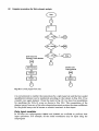
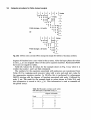
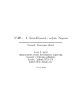
Figure 20.1 shows a simplified schematic for a typical finite element program
system. Each of the modules can in practice be very complex. In the subsequent
introduction 577
Data Input Module
(Preprocessor)
I
Solution and
Output Module
(Postprocessor)
(*)
Fig. 20.1 Simplified schematic of finite element program.
sections we shall discuss in some detail the programming aspects for each of the
modules. It is assumed that the reader is familiar with the finite element principles
presented in this book, linear algebra, and programming in either Fortran or C.
Readers who merely intend to use the program may find information in this chapter
useful for understanding the solution process; however, for this purpose it is only
necessary to read the user instructions available from the web site where the program
is downloaded.
This chapter is divided into seven sections. Section 20.2 describes the procedure
adopted for data input, necessary to define a finite element problem and basic instructions for data file preparation. The data to be provided consists of nodal quantities
(e.g., coordinates, boundary condition data, loading, etc.) and element quantities
(e.g., connection data, material properties, etc.).
Section 20.3 describes the memory management routines.
Section 20.4 discusses solution algorithms for various classes of finite element
analyses. In order to have a computer program that can solve many types of finite
element problems a command language strategy is adopted. The command language
is associated with a set of compact subprograms, each designed to compute one or
at most a few basic steps in a finite element process. Examples in the language are
commands to form a global stiffness matrix, as well as commands to solve equations,
display results, enter graphics mode, etc. The command language concept permits
inclusion of a wide range of solution algorithms useful in solving steady-state and
transient problems in either a linear or non-linear mode.
In Section 20.5 we discuss a methodology commonly used to develop element
arrays. In particular, numerical integration is used to derive element ‘stiffness’,
‘mass’ and ‘residual’ (load) arrays for problems in linear heat transfer and elasticity.
The concept of using basic shape function routines is exploited in these developments
(Chapters 8 and 9).
In Section 20.6 we summarize methods for solving the large set of linear algebraic
equations resulting from the finite element formulation. The methods may be
divided into direct and iterative categories. In a direct solution a variant of Gaussian
578 Computer procedures for finite element analysis
elimination is used to factor the problem coefficient matrix (e.g., stiffness matrix)
into the product of a lower triangular, diagonal and upper triangular form. A solution (or indeed subsequent resolutions) may then be easily obtained. A direct
solution has the advantage that an a priori calculation may be made on the
number of numerical operations which need to be performed to obtain a solution.
On the other hand, a direct solution results in fill-in of the initial, sparse finite
element coefficient array - this is especially significant in three-dimensional solutions
and results in very large storage and compute times. In the second category.iterative
strategies are used to systematically reduce a residual equation to zero, and thus
yield an acceptable solution to the set of linear algebraic equations. The scheme
discussed in this chapter is limited to solution of symmetric equations by a preconditioned conjugate gradient method.
20.2 Data input module
The data input module shown in Fig. 20.1 must obtain sufficient information to
permit the definition and solution of each problem by the other modules. In the
program discussed in this book the data input module is used to read the necessary
geometric, material, and loading data from a file or from information specified by
the user using the computer keyboard or mouse. In the program a set of dynamically
dimensioned arrays is established which store nodal coordinates, element connection
lists, material properties, boundary condition indicators, prescribed nodal forces and
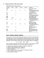
displacements, etc. Table 20.1 lists the names of variables which are used in assigning
array sizes for mesh data and Table 20.2 indicates some of the main arrays used to
store mesh data.
Table 20.1 Control parameters
Variable name
Description
Default
NUMNP
Number of nodal points in mesh
Number of elements in mesh
Number of material sets in mesh
Spatial dimension of mesh
Number of degrees of freedom per node (maximum)
Number of nodes per element (maximum)
Number of material property values per set
0
0
0
none
none
none
200
NUMEL
NUMMAT
NDM
NDF
NEN
NDD
Table 20.2 Variable names used for data storage
Variable name (dimension)
Type
Description
ID (NDF ,NUMNP , 2 )
IE(NIE,NUMMAT)
Integer
Integer
IX(NEN1,NIIMEL)
D (NDD ,NUMMAT)
F (NDF,"PI
2)
X(NDM, "P)
Integer
Real
Real
Real
(I) Boundary codes; (2) Equation numbers
Element pointers for degrees of freedom, history
pointers, material set type, etc.
Element connections, set flag, etc.
Material property data sets
(I) Nodal forces; (2) and displacements
Nodal coordinates
Data input module 579
The notation used for the arrays often differs from that used in the text. For
example, in the text it was found convenient to refer to nodal coordinates as x i , yi,
zi,whereas in the program these are called X( 1, i ) , X(2, i), X ( 3 , i) , respectively.
This change is made so that all arrays used in the program can be dynamically
allocated. Thus, if a two-dimensional problem is analysed, space will not be reserved
for the X ( 3 , i ) coordinates. Similarly the nodal displacements in the text were
commonly named ai; in the program these are called U ( 1 , i ) , U(2, i ) , etc., where
the first subscript refers to the degrees of freedom at a node (from I to NDF).
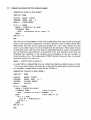
20.2.1 Control data and storage allocation
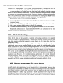
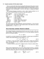
The allocation of the major arrays for storage of mesh and solution variables is
performed in a control program as indicated in Fig. 20.2. Since a dynamic
memory allocation is used it is not possible to establish absolute values for the
maximum number of nodes, elements or material sets. The value for the parameter
NUM-MR defines the amount of memory available to solve a given problem and is
assigned to the main program module; however, if this is not sufficient an error
message is given and the program stops execution.
To facilitate the allocation of all the arrays data defining the size of the problem is
input by the control program as shown schematically in Fig. 20.2. The required data is
shown in Table 20.1; however, the number of nodes, elements and material sets may
be omitted and FEAPpv. f will use the subsequent input data to determine the actual
size required. Using the size data the remaining mesh storage requirements are
determined and allocated by the control program.
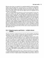
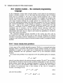
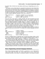
20.2.2 Element and coordinate data
After a user has determined the mesh layout for a problem solution the data must be
transmitted to the analysis program. As an example consider the specification of the
nodal coordinate and element connection data for the simple two-dimensional (NDM =
2) rectangular region shown in Fig. 20.3, where a mesh of nine four-node rectangular
elements (NUMEL = 9 and NEN =4) and 16 nodes (NUMNP = 16) has been indicated. To
describe the nodal and element data, values must be assigned to each X ( i , j) for
i = 1,2 a n d j = 1 to 16 and to each IX(k,n) for k = 1 to 4 and n = 1 to 9. In the
definition of the coordinate array X, the subscript i indicates the coordinate direction
and the subscriptj the node number. Thus, the value of X ( 1 , 3 ) is the x coordinate for
node 3 and the value of X(2,3) is the y coordinate for node 3. Similarly for the
element connection array IX the subscript k is the local node number of the element
and n is the element number. The value of any IX(k,n) (for k less than or equal to
NEN) is the number of a global node. Values of k larger than NEN are used to store
other data. The convention for the first local node number is somewhat arbitrary.
The local node number 1 for element 3 in Fig. 20.3 could be associated with global
node 3, 4, 7, or 8. Once the first local node is established the others must follow
according to the convention adopted for each particular element type. For example,
580 Computer procedures for finite element analysis
Fig. 20.2 Control program flow chart.
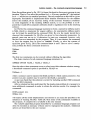
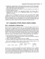
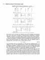
it is conventional to number the connections by a right-hand rule and the four-noded
quadrilateral element can be numbered according to that shown in Fig. 20.4. If we
consider once again element 3 from the mesh in Fig. 20.3 we have four possibilities
for specifying the IX(k,3) array as shown in Fig. 20.4. The computation of the
element arrays from any of the above descriptions must produce the same coefficients
for the global arrays and is known as element invariance to data input.
Data input modules
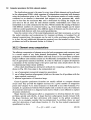
In FEAPpv two subprograms PINPUT and TINPUT are available to perform data
input operations. For example, all the nodal coordinates may be input using the
subprogram
Data input module
Fig. 20.3 Simple two-dimensional mesh.
Fig. 20.4 Typical four-noded element and numbering options.
581
582
Computer procedures for finite element analysis
SUBROUTINE XDATA (X ,NDM,NUMNP)
IMPLICIT NONE
LOGICAL ERRCK, PINPUT
INTEGER NUMNP, NDM , N
REAL*8 X (NDM,NUMNP)
DO N = 1,NUMNP
ERRCK = PINPUT(X(1,N) ,NDM)
IF(ERRCK) THEN
STOP ' Coordinate error: Node:',N
ENDIF
END DO ! N
END
The above use of the PINPUT routine obtains NDM values from each record and assigns
them to the coordinate components of node N. The data input routines obtain their
information from the current input file specified by a user. The routines are also
used in cases where input is to be provided from the keyboard. These input all data
in character mode, and parse the data for embedded function names or parameters
(use of functions and parameters is described in the user manual). Users who are
extending the capability of the program are encouraged to use the routines to
avoid possible errors. The subprogram TINPUT permits character data to precede
numerical values use is given as
ERRCK
=
TINPUT(TEXT,M,DATA,N)
in which TEXT is a CHARACTER*15 array of size M and DATA is a REAL*8 array of size N.
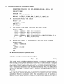
For cases where integer information is to be input the information must be moved.
For example, a simple input routine for the IX data is
SUBROUTINE IXDATA(IX,NENl ,NUMEL)
IMPLICIT
NONE
LOGICAL
INTEGER
INTEGER
REAL*8
ERRCK, PINPUT
NUMEL, NENI , N, I
IX(NEN1,NUMEL)
RIX ( 16)
DO N = 1,NUMEL
ERRCK = PINPUT(RIX,NENI)
IF(ERRCK) THEN
! Stop on error
STOP ' Connection error: ELEMENT:',N
! Move data to IX
ELSE
DO I = 1,NENl
IX(1,N) = NINT(RIX(1))
END DO ! I
ENDIF
END DO ! N
END
Data input module 583
While the above form is not optimal it is an expedient method to permit the arbitrary
mixing of real and integer data on the same record. In the above two examples the
node and element numbers are associated with the record number read. The form
used in the routines supplied with FEAPpv include the node and element numbers
as part of the data record. In this form the inputs need not be sequential nor all
data input at one instance.
For a very large problem the preparation of each node and element record for the
mesh data would be very tedious; consequently, some methods are provided in
FEAPpv to generate missing data. These include simple interpolation between missing
numbers of nodes or elements, use of super-elements to perform generation of blocks
of nodes and elements, and use of blending function methods. Even with these aids
the preparation of the mesh data for nodes and coordinates can be time consuming
and users should consider the use of mesh generation programs such as GiD3 to
assist in this task. Generally, however, the data input scheme included in the program
is sufficient to solve academic and test examples. Moreover the organization of the
mesh input module (subprogram PMESH) is data driven and permits users to interface
their own program directly if desired (see below for more information on adding
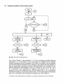
features). The data-driven format of the mesh input routine is controlled by keywords
which direct the program to the specific segment of code to be used. In this form each
input segment does not interact with any of the others as shown schematically in the
flow chart in Fig. 20.5.
20.2.3 Material property specification - multiple element
routines
The above discussion considered the data arrays for nodal coordinates and element
connections. It is also necessary to specify the material properties associated with
each element, loadings, and the restraints to be applied to each node.
Each element has associated property sets, for example in linear isotropic elastic
materials Young’s modulus E and Poisson’s ratio Y describe the material parameters
for an isotropic state. In most situations several elements have the same property
sets and it is unnecessary to specify properties for each element individually. In
the data structure used in FEAPpv an element is associated with a material set by
a number on the data record for each element. The material properties are then
given once for each number. For example, if the region shown in Fig. 20.3 is all
the same material, only one material set is required and each element would reference this set. To accommodate the storage of the material set numbers the IX
array is increased in size to NENl entries and the material set number is stored in
the entry IX(NEN1,n) for element n. In FEAPpv the material properties are stored
in the array D (NDD,NUMMAT), where NUMMAT is the number of different material
sets and NDD is the number of allowable properties for each material set (the default
for NDD is 200).
Each material set defines the element type to which the properties are to be assigned.
In realistic engineering problems several element types may be needed to define the
problem to be solved. A simple example involving different element types is shown in
584 Computer procedures for finite element analysis
Fig. 20.5 Flow chart for mesh data input.
Fig. 1.4(a) in Chapter 1 where elements 1, 2, 4, and 5 are plane stress elastic elements
and element 3 is a truss element. In this case at least two different types of element
stiffness formulations must be computed. In FEAPpv it is possible to use ten different
user provided element formulations in any ana1ysis.t The program has been designed so
that all computations associated with each individual element are performed in one
element subprogram called ELMTnn, where M is between 01 and 10 (see Sec. 20.5.3
for a discussion on the organization of ELMTnn). Each element type to be used is
specified as part of the material set data. Thus if element type 1, e.g., computations
performed by ELMTO1,is a plane linear elastic three- or four-noded element and element
type 4 is a truss element, the data given for example Fig. 1.4(a) would be:
t In addition, some standard element formulations are provided as described in the user instructions.
Data input module 585
(a) Material properties
Material
set number
Element
type
Material property
data
(b) Element connections
Element
Material set
Connection
1
2
2
2
134
3
1
2
4
5
2
142
25
3614
4185
where E is Young’s modulus, v is Poisson’s ratio and A is area. Thus, elements 1,2,4,
and 5 have material property set 2 which is associated with element type 1 and element
3 has a material property set 1 which is associated with element type 4.It will be seen
later that the above scheme leads to a simple organization of an element routine which
can input material property sets and perform all the necessary computations for the
finite element arrays.
More sophisticated schemes could be adopted; however, for the educational and
research type of program described here this added complexity is not warranted.
20.2.4 Boundary conditions - equation numbers
The process of specifying the boundary conditions at nodes and the procedure for
imposing specified nodal displacements is closely associated with the method adopted
to store the global solution matrix, e.g., the stiffness matrix. In FEAPpv the direct
solution procedure included uses a variable band (profile) storage for the global
solution matrix. Accordingly, only those coefficients within the non-zero profiles
are stored.
While the nodal displacements associated with boundary restraints may be
imposed using the ‘penalty’ method described in Chapter 1, a more efficient direct
solution results if the rows and columns for these equations are deleted. As an
example consider the stiffness matrix corresponding to the problem shown in
Fig. 1.1; storing all terms within the upper profile leads to the result shown in
Fig. 20.6(a) and requires 54 words, whereas if the equations corresponding to the
restrained nodes 1 and 6 are deleted the profile shown in Fig. 20.6(b) results and
requires only 32 words. In addition to a reduction in storage requirements, the
computer time to solve the equations is also reduced.
To facilitate a compact storage operation in forming the global arrays, a boundary
condition array is used for each node. The array is named I D and is dimensioned as
shown in Table 20.2. During input of data, degrees of freedom with known value or
where no unknown exists have a non-zero value assigned to I D (i ,j ,1>.All active
586 Computer procedures for finite element analysis
Fig. 20.6 Stiffness matrix: (a) total stiffness storage; (b) storage after deletion of boundary conditions.
degrees of freedom have a zero value in the I D array. After the input phase the values
in I D (i,j ,2) are assigned values of the active equation numbers. Restrained DOFs
have zero (or negative) values.
Table 20.3 shows the I D values for the example shown in Fig. l.l(a), where it is
evident that nodes 1 and 6 are fully restrained.
The numbers for the equations associated with unknowns are constructed from
Table 20.3 by replacing each non-zero value with a zero and each zero value by
the appropriate equation number. In FEAPpv this is performed by subprogram
PROFIL starting with the degrees of freedom associated with node 1 followed by
node 2, etc. The result for the example leads to values shown in Table 20.4, and
this information is stored in I D ( i , j ,2). This information is used to assemble all
the global arrays.
Table 20.3 Boundary restraint code values
after data input of problem in Fig. 1 . 1
Degree of freedom
Node
1
2
1
2
3
5
1
0
0
0
0
1
0
0
0
0
6
1
1
4
Data input module 587
Table 20.4 Compacted equation numbers
for problem in Fig. 1.1
Degree of freedom
Node
1
2
1
0
2
3
1
0
2
3
4
4
5
5
7
0
6
8
0
6
The above scheme may be modified in a number of ways for either efficiency or to
accommodate more general problems. For problems in which the node numbers are
input in an order which creates a very large profile it is advisable to employ a program
to renumber the nodes for better efficiency (often called bandwidth minimization
schemes). Using the renumbered node order the equation numbers may then be
constructed.
The solution of mixed formulations which have matrices with zero diagonals
requires special care in solving for the parameters. For example in the q, formulation discussed in Sec. 11.2 it is necessary to eliminate all qi parameters associated
with each & parameter when a direct method of solution without pivoting is used
(e.g., those discussed in Sec. 20.6.1). This may be achieved by numbering the
I D ( i , j ,2) entries so that qi have smaller equation numbers than the one for the
associated &.
The equation number scheme may be further exploited to handle repeating boundaries (see Chapter 9, Sec. 9.18) where nodes on two boundaries are required to have
the same displacement but the value is unknown. This is accomplished by setting the
equation numbers to the same value (and discard the unused ones). Similarly, regions
may be joined by assigning nodes with the same coordinate values the same equation
numbers.
All modifications of the above type must be performed prior to computing the
profile of the global matrix.
20.2.5 Loading - nodal forces and displacements
In FEAPpv the specified nodal forces and displacements associated with each degree
of freedom are stored in the array F (NDF, NUMNP ,2). The specified force values for
degree of freedom i at node j are retained in F ( i , j , I ) and specified values for the
corresponding specified displacements in F ( i ,j ,2). The actual value to be used
during each phase of an analysis depends on the current value stored in
I D ( i , j ,1). Thus if the value of the I D ( i , j ,1) is zero a force value is taken from
F ( i , j ,1) whereas if the value is non-zero a displacement value is taken from
F ( i ,j ,2). For the example of Fig. 1.1, an 0.01 settlement of the node 1 can be
input by setting F(1,2,2) = -0.01, where it is assumed that the second degree of
588 Computer procedures for finite element analysis
freedom is a displacement in the vertical direction. Similarly, a horizontal force at
node 4 can be specified by setting F ( 1 , 4 , 1 > = 5, (i.e., X4 in the figure).
In many problems the loading may be distributed and in these cases the loading
must first be converted to nodal forces. In FEAPpv there are some provisions included
to perform the computation automatically. Users may develop additional schemes for
their own problems and add a new input command in the subprogram PMESH.Other
options could also be added to compute necessary nodal quantities.
The necessary steps to add a feature in PMESH are:
1. Increase the dimensioned size of the array WD which is a character array to store the
command names.
2. Set the value of LIST in the DATA statement to the new number of entries in WD.
3. Add a new statement label entries to the GO TO statement.
4. For each statement label entry add the program statements for the new feature.
The specific instructions to prepare data for FEAPpv are contained in the user
manual available at the publisher’s web site.
20.2.6 Mesh data checking
Once all the data for the geometric, material and loading conditions are supplied
FEAPpv is ready to initiate execution of the solution module; however prior to this
step it is usually preferable to perform some checks on the input data (and any
generated values).
After the mesh is input the program will pass to solution mode. During solution
additional arrays may be required which can also exceed the available space in the
blank common. The most intensive storage requirement is for the global coefficient
matrix for the set of linear algebraic equations defining the nodal solution parameters.
In direct solution mode a variable band, profile solution scheme is used for simplicity.
The solver has the capability of solving both symmetric and unsymmetric coefficient
arrays and this is generally adequate for one- and two-dimensional problems of
moderate size. However, for three-dimensional applications the storage demands
for the coefficient matrix can exceed the capabilities of even the largest computers
available at the time of writing this volume. Thus, an alternative iterative scheme is
included in FEAPpv using a simple preconditioned conjugate gradient solver.
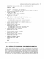
20.3 Memory management for array storage
A single array is partitioned to store all the main data arrays, as well as other arrays
needed during the solution and output phases. This is accomplished using a data
management system which can define, resize or destroy an integer or real array. Depending on the computer system used real arrays may be defined in the main program
module FEAPpv. F in either single precision or double precision form. Using the data
management system each array indicated in Table 20.2 is dynamically dimensioned to
the size and precision required for each problem. The result is a set of pointers defining
Memory management for array storage
the location in a single array located in blank common. Blank common is defined as
REAL*8 HR
INTEGER
MR
COMMON
HR(1) ,MR(NUM-MR)
and pointers are assigned into the array NP stored in the named common POINTERS
given by
INTEGER
NP
COMMON /POINTERS/ NP (NUM-NP)
The size of each array is defined by parameters NUM-MR and “M-NP. While not
strictly defined by programming standards the above size for HR is not limited to 1.
By working outside the array bound real arrays may be defined up to size NUM_MR/2
for the double precision indicated. Using this artifice of pointers subroutines may be
called as
CALL SUBX(MR(NP(5)),
HR(NP(3311,
.. .
1
where the first argument is integer and the second real. The subroutine would then
read
SUBROUTINE SUBX(I1, R1,
. .. .
and real names associated with each array as determined by a programmer. At this
stage the missing ingredient is assignment of values to each specific pointer. In
FEAPpv this is accomplished by the subprogram PALLOC. This logical function
subprogram associates a number with a name for each variable to be defined,
changed or deleted. Each programmer must use a listing of this routine to understand
which variable is being defined and whether the variable is to be real or integer. A
specification of an array action is accomplished using the assignment statement
SETVAL
=
PALLOCC NUM , NAME , LENGTH , PRECISION )
For example the statement
SETVAL
=
PALLOCC 43 , ‘X’ , NDM*NUMNP , 2 )
defines the real array for the nodal coordinates to have a size as indicated in Table
20.2. Similarly, the statement
SETVAL = PALLOCC 33 , ‘IX’ , NENI*NUMEL , 1 )
defines an integer array for the element connection array. Repeating the use of the
allocation statement with a different size (either larger or smaller) will redefine
the size of the array. Similarly, use of the statement with a zero (0) size deletes the
array from the allocation table. Accordingly, use of
SETVAL
=
PALLOCC 33 , ‘IX’ , 0 , I
)
would destroy the storage (and values) for the connection data. Thus, using the
memory management scheme above it is possible to redefine a mesh in an adaptive
solution scheme to add or delete specific element data. Alternatively, data may be
used in a temporary manner by allocating and then deleting after use.
589
590 Computer procedures for finite element analysis
20.4 Solution module
language
- the command programming
At the completion of data input and any checks on the mesh we are prepared to
initiate a problem solution. It is at this stage that the particular type of solution
mode must be available to the user. In many existing programs only a small
number of solution modes are generally included. For example, the program may
only be able to solve linear steady-state problems, or in addition it may be able to
solve linear transient problems for a single method. In a research mode or indeed
in practical engineering problems fixed algorithm programs are often too restrictive
and continual modification of the program is necessary to solve specific problems
that arise - often at the expense of features needed by another user. For this
reason it is desirable to have a program that has modules for various algorithm
capabilities and, if necessary, can be modified without affecting other users’
capabilities. The program form that we discuss here is basic and the reader can
undoubtedly find many ways to improve and extend the capabilities to be able to
solve other classes of problems.
The command language concept described in this section has been used by
the authors for more than 20 years and, to date, has not inhibited our research
activities by becoming outdated. Applications are routinely conducted on personal
computers and workstations using an identical program except for graphical display
modules.
20.4.1 Linear steady-state problems
A basic aspect of the variable algorithm program FEAPpv is a command instruction
language which is associated with specific program solution modules for specific
algorithms as needed. A user needs only to understand the association between
specific commands and the operations carried out by the associated solution
modules.
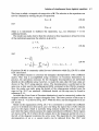
In a steady-state problem we are required to solve the problem given, for example,
by
r(k) = f - Ka(k)
(20.1)
where k is an index related to the solution iteration number. We call
the residual of
the problem for iteration k and note that a solution results when it is zero. In a datadriven solution mode using the command language of FEAPpv the formulation of
Eq. (20.1) is given by the command FORM, which is a mnemonic for form residual.
In addition an incremental form of the solution of Eq. (20.1) is adopted in
FEAPpv. Accordingly we let
= a(k) + Aa(k)
(20.2)
(20.3)
Solution module - the command programming language 591
Since the problem given by Eq. (20.1) is linear this iterative form must converge in one
iteration. That is, if we solve the problem fork = 0 for any specified a('), the residual
fork = 1 will be zero (to machine precision). The only exceptions to this will be: (a) an
improperly formulated or implemented finite element formulation for the stiffness
and/or the residual; (b) an incorrect setting of the necessary boundary conditions
to avoid singularity of the resulting stiffness matrix; or (c) the problem is so illposed that round-off in computer arithmetic leads to significant error in the resulting
solution.
In FEAPpv the command language statement to form a symmetric stiffness matrix
is TANG, which is a mnemonic for tangent stzflness. An unsymmetric stiffness matrix
can be formed by specifying the command UTAN. By now the reader should have
observed that commands for FEAPpv are given by four-character mnemonics. In
general, users can use up to 14 characters to issue any command, however, only
the first four are interpreted by the program. Thus, if a user desires, the command
to form the tangent may be given as TANGENT. Finally, to solve the systems of
equations given by Eq. (20.3)the command SOLV is used. Thus to solve a steadystate problem the three commands issued are:
TANGent
FORM
SOLVe
The first two commands can be reversed without affecting the algorithm.
The basic structure for all command language statements is:
COMMAND OPTION VALUE-I VALUE-2 VALUE-3
Since the above three statements occur so often in any finite element solution strategy
a shorthand command option is provided in FEAPpv as
TANGent,,l
where a comma is used to separate the fields and leave a blank option parameter. Any
positive non-zero number may be used for the VALUE-I parameter.
A user can check that the solution is correct by including another FORM command
after the SOLV statement.
After a solution has been performed for the steady-state problem it is necessary to
issue additional commands in order to obtain the solution results. For example, the
commands
DISPlacement ALL
STRESS ALL
will output all the nodal displacements and stresses in an outputjle specified at the
initiation of running FEAPpv. Table 20.5 lists some of the commands available in
the program. A complete list is available in the user manual.
The variable algorithm program described by a command language program can
often be extended as necessary without need to reprogram the modules. Additional
options are described in the user manual.
592
Computer procedures for finite element analysis
Table 20.5 Partial list of solutions commands
Command
Option
Value-1
Value2
Value-3
CHECk
Description
Perform check of mesh
(ISW = 2)'
DISP
ALL
N1
N2
N3
v1
DT
FORM
Output displacement for nodes
N 1 to N 2 at increments of N 3
A L L outputs all
Set time increment to V 1
Form equation residual
(ISW = 6)
LOOP
N
MESH
NEXT
PLOT
OPTION
REAC
ALL
N1
N2
N3
Loop N times all instructions
to a matching NEXT command
Input changes to mesh
End of LOOP instruction
Enter graphical mode
or perform command O P T I O N
Output reactions at nodes
N1 to N 2 at increments of N 3
A L L outputs all
(ISW = 6)
SOLV
STRE
ALL
N1
N2
N3
Solve for new solution
increment (after FORM)
Output element variables
N 1 to N 2 at increments of N 3
ALL outputs all
(ISW = 4)
TANGent
N1
Form symmetric tangent
Solve if N 1 positive
(ISW = 3)
TIME
TOL
UTAN
Advance time by D T value
Set solution tolerance to V i
Form unsymmetric tangent
v1
N1
(ISW = 3)
20.4.2 Transient solution methods
The integration of second-order differential equations of motion for time-dependent
structural systems can be treated using the command language program. The firstorder differential equations resulting from the heat equation may also be similarly
integrated. For the transient second-order case the residual equation is modified to
r(k) = f - Ka(k)- Ci(&)-
(20.4)
where C and M are damping and mass matrices, respectively, and a and a are velocity
and acceleration, respectively. To solve this problem it is necessary to:
1. specify the time integration method to be used (see Chapter 18);
2. specify the time increment for the integration;
3. specify the number of time steps to perform;
4. form the residual
5 . form the tangent matrix for the specific time integration method;
6 . solve the equation for each time step;
7. report answers as needed.
Solution module - the command programming language 593
As an example we consider the Newmark method (GN22) as described in Chapter
18, Sec. 18.33. Using Eq. (18.12) we can define the updates at iteration k as
(20.5)
(20.6)
where a,,, and an+, are expressed in terms of solution variables at time n. These
equations may also be written in an incremental form as
(20.7)
(20.8)
Comparing Eq. (20.7) with Eq. (20.3) we obtain
Aafl
= ip2At2Aafi
(20.9)
Similarly
(20.10)
Thus, selecting the incremental nodal displacements as the primary unknown, the
residual equation for k 1 may be written as
+
,dk+l)
= r(k)- K*Aan+
( k )1
(20.11)
where
K* = c ~ K
+ c ~ +C c ~ M
(20.12)
with
c, =
I
(20.13)
2
c3 = -
P2At2
obtained from the relations between the incremental displacement, velocity and
acceleration vectors. As we have noted in Chapter 18 the changing of the primary
unknown from displacement to acceleration or velocity or, indeed, changing the
integration algorithm from Newmark to any other method only changes the residual
equation by the parameters ciwhich define the tangent matrix K*. The other changes
from different integration algorithms appear in the number of vectors required for the
algorithm and the way they are initialized and updated within each time increment.
In program FEAPpv the parameters ci are passed to each element routine as
CTAN ( i > together with the values of the localized nodal displacement, velocity and
acceleration vectors. This permits an element module to be programmed in a general
manner without knowing which integration method will be used during the solution
specified in the command language instructions. In Sec. 20.5 we will discuss the steps
needed to program the residual terms, as well as the stiffness and mass terms needed to
form the global tangent matrix.
594 Computer procedures for finite element analysis
Here we note also that the steady-state algorithm discussed in the previous section
merely requires that the velocity and acceleration vectors and the parameters c2 and c3
be set to zero before calling an element module. Similarly, for a first-order system the
acceleration vector and parameter c3 are set to zero prior to entering the element
module.
The command language instructions to solve a linear transient problem over 50
time steps in which all results are reported at each time is given as
TRANS,NEWMark
DT, ,0.024
TANG
LOOP,time,50
FORM
SOLVe
DISP,ALL
STRE,ALL
NEXT,time
Selects Newmark Method
Sets time increment to 0.024
Form tangent matrix
Loop 50 times to NEXT
Form residual
Solve equations
Output nodal displacements
Output element variables
End of LOOP
The issuing of the instructions TRANsient causes the parameters ci to be set for the
Newmark method. The default for the transient option is the steady-state solution
algorithm with c1 = 1 and c2 = c3 = 0.
20.4.3 Non-linear solutions: Newton's methods
The command language programming instructions may also be used to solve nonlinear problems. For example, the steady-state set of non-linear algebraic equations
given by the residual equation
r(') = f - P(a('))
(20.14)
in which P is a non-linear function of a is considered. A solution may be obtained by
writing a linear approximation for the residual at k 1 as
+
r(k+l)
- K (T~ ) A ~ ( W = 0
(20.15)
in which KT is some non-singular coefficient matrix used to obtain the increments
Aa,,).. Now the update for a('+]) using Eq. (20.2) will not in general make r('+l)
zero in one iteration.
A common method to generate the coefficient matrix is Newton's method where
(20.16)
When properly implemented the norm of the residual should converge at a quadratic
asymptotic rate. Thus if Ilrl( is the norm of the residual then for an approximation
close to the solution the ratios for two successive iterations should be
(20.17)
Solution module - the command programming language 595
In general, this is the best one can obtain with the type of algorithm given by Eq.
(20.15).
In FEAPpv a norm of the solution is computed for each iteration and a check of the
current norm versus the initial value is performed as indicated in Eq. (20.17). Once the
value of the ratio of the norm is below a specified tolerance, convergence is assumed.
The solution tolerance is set using the command language instruction TOL as indicated
in Table 20.5 (the default value for the norm is
The instructions to perform a
solution using the algorithm indicated in Eq. (20.15) is given by
LOOP,iteration,lO
TANG, ,I
NEXT,iteration
! Perform a maximum of IO iterations
! Compute tangent, residual and s o l v e
! End for LOOP instruction
Once the ratio of the norms is reached, FEAPpv will exit the iteration loop and
execute the instruction following the NEXT statement. If the element module used
has a tangent matrix computed using Eq. (20.16) the asymptotic behaviour of
Newton’s method should be attained. Failure to achieve a quadratic rate of
convergence during the last few iterations indicates an incorrect implementation in
the element module, a data input error, or extreme sensitivity in the formulation
such that round-off prevents the asymptotic rate being reached. One can never
achieve convergence beyond that where the round-off limit is reached.
An alternative to the above program is the modified solution method in which the
tangent is used from an earlier state. For example, the command language instruction
set
TANG
LOOP,iteration,10
FORM
SOLVe
NEXT,iteration
!
!
!
!
!
Compute tangent
Perform a maximum of 10 iterations
Compute residual
Solve equations
End for LOOP instruction
executes a modified Newton’s algorithm and, for general non-linear systems, results
in less than a quadratic asymptotic rate of convergence (generally linear or less, so
that if iteration k gives a ratio of order
iteration k 1 gives about
The execution of each TANG, W A N , FORM, etc. instruction uses the current problem
type and time increment to define the parameters ci along with the current solution
values for a@),a@)and a@)to calculate a tangent, residual, etc., respectively.
Many additional solution algorithms may be established using the commands
available in the program. Some of these are discussed in the user manual where
topics ranging from time-dependent loading to general transient, non-linear solution
strategies included in FEAPpv are described. Authors may be found in Volume 2.
+
20.4.4 Programming command language statements
The command language module for FEAPpv is contained in a set of subprograms
whose names begin with PMAC. The routine PMACR calls the other routines and
establishes the limits on the number of commands available to the program. Included
596 Computer procedures for finite element analysis
SUBROUTINE UMACRl(LCT,CTL,PRT)
IMPLICIT NONE
C
C
C
C
Inputs:
LCT
- Command character parameters
CTL(3) - Command numerical parameters
- Flag, output if true
PRT
c
outputs:
N.B. Users are responsible for command actions.
C
IMPLICIT NONE
LOGICAL PCOMP,PRT
CHARACTER LCT*15
REAL*8
CTL(3)
CHARACTER
UCT*4
COMMON /UMACl/ UCT
C
C
Set command word to user selected name
IF(PCOMP(UCT,’MACI’,4)) THEN
UCT = ‘xxxx’
RETURN
ELSE
Implement user solution step
ENDIF
END
Fig. 20.7 Structure of a user command subprogram.
in the current command list is an option to access a set of user subprograms named
UMACRn where n ranges from 1 to 5. Each user subprogram has a structure as shown in
Fig. 20.7. A user is required to select a four character name for xxxx which does not
already exist in the command list in PMACR and to program the desired solution step.
It should be noted that all arrays identified in the subprogram PALLOC can be
accessed directly using the data management system described in Sec. 20.3. In
addition data may be assigned to space in memory using the TEMPn array names
that are also available in PALLOC. Thus it is not necessary to pass the names of
arrays through the argument list of the subprograms UMACRn.Quite general routines
can be created using these routines; however, if a more involved command is deemed
necessary by a user the routines PMACRn may be modified to add additional instructions. This is not an option which should be considered without a thorough study
of the new solution option needed, as well as, options already available in the
commands included.
If it is decided to modify the PMACRn routines it is necessary to:
1. Increase the size of the WD array in subprogram PMACR by the number of commands
to be added.
Computation of finite element solution modules 597
2. Add the new command name to the list in the data statement for WD in subprogram
PMACR noting which of the routines PMACRn will have the solution module added
(the continue labels indicate the value of n).
3. Increase the value of the variable NWDn in the data statement by the number of
commands added for each n.
4. Add the solution module to the subprograms PMACRn. This requires either a
modification of a GO TO or an IF-THEN-ELSE program form in addition to
adding the statements.
Again users are reminded that extreme care must be exercised when adding
commands in this way. Despite the fact that each command involves a specific
solution step or steps there are some interactions between instructions that exist. If
these are changed in any way the program may not function properly after new
commands are added. This is particularly true for setting the parameters NWDn since
if these are not correct transfer to incorrect locations in the list can occur.
20.5 Computation of finite element solution modules
20.5.1 Localization of element data
When we want to compute an element array, e.g., an element stiffness matrix, S , or an
element load or residual vector, P, we only need those quantities associated with the
one element in question. The nodal and material quantities that are required can be
determined from the node and material set numbers stored in the IX array for each
element. In the program FEAPpv the necessary values are moved from each global
array to a set of local arrays before the appropriate element routine, ELMTnn, is
called. The process will be called localization. The quantities that are localized are:
1. nodal coordinates which are stored in the local array XL (NDM,NEN) ;
2. nodal displacements, displacement increments, velocity and acceleration which are
stored in the array UL (NDF,NEN , 5 ) ;
3. nodal T-variables which are stored in the array TL(NEN1;
4. equation numbers for assembly which are stored in the destination array LD(NEN) .
The LD array described in Step 4 above is used to map the element arrays to the
global arrays. Accordingly, for the following element array:
the term S (i ,j) would be assembled into the global coefficient array (e.g., stiffness
matrix) in the position corresponding to row LD(i) and column LD(j). Similarly,
P ( i ) would be assembled into the position corresponding to the LD(i) value. That
is, the LD array contains the equation numbers of the global arrays. The LD(i) assignment of the degrees of freedom for each node is made using the data stored in the
ID(j ,k,2) array as shown in Table 20.2.
598 Computer procedures for finite element analysis
The localization process is the same for every type of finite element and is performed
in the subprogram PFORM, which organizes all computations associated with elements
using the connections given in the IX array. The maximum number of nodes actually
connected to an element is determined and assigned to the parameter NEL, which
may be less than the maximum NEN, and is determined by finding the largest nonzero entry in the IX array for each element number. Intermediate zero values are
interpreted as no node connected. In this way FEAPpv permits the mixing of elements
with different numbers of connected nodes, e.g., three-noded triangles can be mixed
with four-noded quadrilaterals. Also different types of elements can be mixed such as
two-noded shell elements with four-noded quadrilaterals.
Since the current value of the nodal displacements and their increments, as well as
the nodal velocities and accelerations for transient problems, is localized for all
element computations, the program can be used to solve non-linear problems. This
is, in fact, the only additional information required over that needed to solve linear
problems and will be discussed further in Volume 2.
20.5.2 Element array computations
The efficient computation of element arrays (in both programmer and computer time)
is a crucial aspect of any finite element development. The development of subprograms to evaluate element stiffness and load arrays (or for non-linear problems
tangent stiffness and residual arrays) can be efficiently accomplished by a combination of appropriate numerical methods. In order to illustrate a typical development
a statement of the essential steps is first given and then some details shown for the
two-dimensional linear elastic problem.
A flow chart describing two alternative methods for computing a stiffness matrix is
shown in Fig. 20.8. Key steps in the computation are:
1. use of appropriate numerical integration procedures;
2. use of shape function subprograms (which are the same for all problems with the
same required continuity);
3. efficient organization of numerical steps.
Gauss-Legendre quadrature formulae are usually utilized to compute element
arrays since they provide the highest accuracy for a given number of integration
points (see Chapter 9). In some instances it is desirable to use other formulae. For
example, if a quadrature formula which samples only at nodes is used, the evaluation
of an inertial term leads to a diagonal mass matrix which is more efficient in explicit
dynamics calculations.
Shape function subprograms allow a programmer to develop elements for many
problems quickly and reliably. A shape function subprogram should evaluate both
the shape functions and their derivatives with respect to the global coordinate
frame. As an example consider the two-dimensional C, problem where we need
only first derivatives of each shape function Ni.For the four-noded isoparametric
quadrilateral we have
N i = $ ( l +tiO(l +qiq)
(20.18)
Computation of finite element solution modules 599
Fig. 20.8 Element stiffness matrix computation: (a) general form; (b) form for constant material properties.
<,
where 77 are natural coordinates on the bi-unit square parent element and ti,
vitheir
values at the four nodes.
Using the isoparametric concept we have
x = Nixi
(20.19)
Y = NiYi
600 Computer procedures for finite element analysis
with derivatives given by
(20.20)
(20.21)
where J is the jacobian determinant and ( ),x denotes the partial derivative
a( )/ax,etc. The above relations define the steps for the shape function subprogram
given in Fig. 20.9 where it is assumed that the nodal coordinates have been transferred
to the local coordinate array XL.
This shape function routine can be used for all two-dimensional C, problems which
use the four-noded element (e.g., two-dimensional plane and axisymmetric elasticity,
heat conduction, flow in porous media, fluid flow, etc.). Shape function subprograms
can also be used for the generation of mesh data.4 It is a simple task to extend the
shape function routine to higher order elements (e.g., see the listing for subprogram
SHAP2 in FEAPpv which includes options for up to nine-node quadrilaterals). Using
such routines permits the use of elements which have individual edges with either
linear or quadratic interpolation.
The generation of the matrix products occurring in the stiffness matrix of elasticity
problems deserves special attention since zeros often exist in the B and D matrices.
Several methods can be used to reduce the number of operations performed. The
first is to form explicitly the matrix products. While this involves extra hand computations it is in fact elementary if performed on a nodal basis. For example, consider
the two-dimensional axisymmetric linear elastic problem where
(20.22)
A two-dimensional plane problem may be considered by replacing r , z by x, y and
setting the constant c to zero. For axisymmetry the constant c is unity. For an
isotropic linear elastic material the moduli are given by
(20.23)
where D33is the shear modulus given by (Dll - D12)/2.Thus for a typical nodal pair i
a n d j a contribution to the element stiffness Kij may be computed using
QJ. = DBj
(20.24)
and
K~~=
BTQ~
(20.25)
Computation of finite element solution modules 601
SUBROUTINE SHAPE(SS,XL, J,SHP)
Shape f u n c t i o n r o u t i n e f o r 4-node q u a d r i l a t e r a l
IMPLICIT NONE
INTEGER
REAL*8
DATA
DATA
I1
SS(2)
SI /
TI /
,JJ
,KK
,XL(2,4), J,SHP(3,4) ,SI(4) ,TI@) ,XS(2,2) ,TEMP
-0.5D0, 0.5D0, 0.5D0, -0.5DO/
-0.5D0, -0.5D0, 0.5D0, 0.5DO/
Compute shape f u n c t i o n s and n a t u r a l coordinate d e r i v a t i v e s
DO I1 = 1,4
SHP(1,II) = SI(II)*(0.5DO + TI(II)*SS(2))
SHP(2,II) = TI(II)*(0.5DO + SI(II)*SS(l))
SHP(3,II) = (0.5DO + SI(II)*SS(1))*(0.5DO
END DO ! I1
+ TI(II)*SS(2))
Compute Jacobian and Jacobian determinant
DO I1 = 1,2
DO JJ = 1,2
XS(I1,JJ) = O.ODO
DO KK = 1,4
XS(I1,JJ) = XS(I1,JJ) + XL(II,KK)*SHP(JJ,KK)
END DO ! KK
END DO ! JJ
END DO ! I1
J = XS(l,l)*XS(2,2) - XS(1,2)*XS(2,1)
Transform t o X,Y d e r i v a t i v e s
DO I1 = 1,4
TEMP = ( XS(2,2)*SHP(l,II) - XS(2,1)*SHP(2,II))/J
SHP(2,II) = (-XS(l, 2)*SHP(l, 11) + XS(1,l) *SHP(2,11) )/J
SHP(1,II) = TEMP
END DO ! I1
END
Fig. 20.9 Shape function subprogram for four-noded element.
Thus, using Eqs (20.22) and (20.23) and setting
n . - -CN J.
(20.26)
we obtain
(20.27)
602 Computer procedures for finite element analysis
and finally the stiffness as
Accordingly,for each nodal pair it is required to perform 21 multiplications to form each
K,, whereas formal multiplication of BTDBj including all zero operations would require
48 multiplications. When the element stiffnessmatrix is symmetricit is only necessary to
form the upper or lower triangular parts of K (the other half is formed from the symmetry condition). A typical routine for the stiffness computation is given in Figs 20.10
and 20.11 where it is assumed that the quadrature points are available as SG(1 ,L)
equal to tL,SG(2,L) equal to qL, and SG(3,L) equal to the quadrature weight.
The increments by NDF are to keep the stiffness array stored in nodal order with
NDFxNDF submatrix blocks. This is required by FEAPpv to maintain proper compatibility with the routine used to assemble the global arrays.
SUBROUTINE ELSTIF(D, XL, AXI, NDF,NDM,NST, S)
IMPLICIT NONE
LOGICAL
INTEGER
REAL*8
REAL*8
REAL*8
AX1
II,Il, JJ,Jl, L, LINT, NDF,NDM,NST
DV, Dll,Dl2,D33, J, R
D(*), XL(NDM,4), S(NST,NST)
SG(3,4), SHP(3,4), Q(4,2), N(4)
CALL INT2D(2,LINT, SG) ! Set up 2x2 quadrature points
c
Do numerical integration
DO L = 1,LINT
CALL SHAPE(SG(1,L) ,XL, J,SHP)
DV = J*SG(3,L)
! SG(3,L)
D11 = D(l)*DV
! D(1) is
D12 = D(2)*DV
! D(2) is
D33 = D(3)*DV
! D(3) is
c
is quadrature weight
D-11 modulus
D-12 modulus
shear modulus
Compute n-i = c*N-i/r
R = O.ODO
! R is radius
DO I1 = 1,4
R = R + SHP(3,II)*XL(l,II)
END DO ! I1
DO I1 = 1,4
IF(AX1) THEN
N(I1) = SHP(S,II)/R
ELSE
N(I1) = O.ODO
ENDIF
END DO ! I1
Fig. 20.10 Element stiffness calculation. Part 1
Computation of finite element solution modules 603
c
Compute Q-j
=
D
*
B-j
Jl = 1
DO JJ = 1,4
Q(1,l) = Dll*SHP(l,JJ) + D12*N(JJ)
Q(2,l) = D12*SHP(l,JJ) + Dl2*N(JJ)
Q(3,l) = D12*SHP(l,JJ) + Dll*N(JJ)
Q(4,l) = D33*SHP(2, JJ)
Q(1,2) = Dl2*SHP(2,JJ)
Q(2,2) = Dll*SHP(2,JJ)
Q(3,2) = D12*SHP(2, JJ)
Q(4,2) = D33*SHP(l,JJ)
Compute stiffness term: k - i j
C
I1 = I
DO I1 = l,JJ
S(I1 ,J1 )
,J1 ) + SHP(1,II)*Q(l,l)+N(II)*Q(3,1)
+ SHP(2,111*Q (4,l)
S(I1 ,JI+l) = S(I1 ,JI+l) + SHP(l,II)*Q(l,2)+N(II)*Q(3,2)
t
+ SHP(2,II) *Q(4,2)
S(Il+l,Jl ) = S(Il+l,Jl ) + SHP(2,II)*Q(2,1)
t
+ SHP(l,II)*Q(4,1)
S(Il+l,Jl+l) = S(Il+l,J1+1) + SHP(2,II)*Q(2,2)
&
+ SHP( 1,111*Q(4,2)
I1 = I1 + NDF
END DO ! I1
Jl = Jl + NDF
END DO ! JJ
END DO ! L
=
S(I1
&
c
Compute lower part by symmetry
DO I1 = 1,NST
DO JJ = 1,11
S(I1,JJ) = S(JJ,II)
END DO ! JJ
END DO ! I1
END
Fig. 20.11 Element stiffness calculation. Part 2.
An extension to anisotropic problems can be made by replacing the isotropic D
matrix by the appropriate anisotropic one and then recomputing the Qj matrix.
The computation of element stiffness matrices for two-dimensional plane and
three-dimensional problems which have constant material properties within an
element can be made more efficient than that given above. This is obtained by
604 Computer procedures for finite element analysis
noting from Appendix B that the internal energy may be written in indicia1 form as
(20.29)
where a, b, c, d are indices from the elasticity equations and range over the space
dimension of the problem and i, j are nodal indices which range from 1 to NEL in
each element. The element stiffness for the nodal pair i, j may be written as
Ki{ = WiDabcd
(20.30)
where
(20.31)
For isotropic materials
(20.32)
where X and p are the Lamk elastic constants which are related to the usual elastic
constants E and p as
vE
E
(l+v)(l-2v)’
2( 1 v)
Thus, the stiffness matrix for an isotropic material is given as
A=
p = -~
+
Using this approach the steps to compute the element stiffness matrix for plane
elasticity are given in Fig. 20.8(b). This procedure for computing stiffness matrices
was noted in reference 5 and for plane problems results in about 25% fewer numerical
operations than the procedure shown in Fig. 20.8(a). In three dimensions the savings
are even greater.
The computation of other element arrays can also be performed using a shape
function routine. For example, the computation of the element consistent and
diagonal mass matrices by the row sum method (see Appendix I) for transient or
eigenvalue computations can be easily constructed. The consistent mass matrix for
two- and three-dimensional problems is obtained from
whereas the diagonal mass is computed from
Mjj=II
p$dV
(20.35 )
ve
In the above I is an identity matrix of size NDM and p is the mass density. A set of
statements to compute the mass matrix for these cases is shown in Fig. 20.12 where
the element consistent mass is stored in the square matrix S and the diagonal mass
matrix is stored in the rectangular array P.
The shape function routine may also be used to compute strains, stresses and
internal forces in an element. The strains at each point in an element may be
Computation of finite element solution modules 605
C
C
S(NST,NST) : Consistent mass array
P(NDM,NEL) : Diagonal mass array
C
Numerical integration loop
DO L = 1,LINT
CALL SHAPE(SG(l,L), XL, J, SHP)
DMASS = RHO* J*SG (3,L)
JI = 1
DO JJ = 1,NEL
JMASS = DMASS*SHP (3, JJ)
P(1,JJ) = P(1,JJ) + JMASS
I1 = I
DO I1 = 1,NEL
S(I1,JI) = S(I1,JI) + SHP((3,II)*JMASS
I1
= I1 + NDF
END DO ! I1
JI = J1 + NDF
END DO ! JJ
END DO ! L
C
Copy using identity matrix
J1 = 0
DO JJ = 1,NEL
DO KK = 2,NDM
P(KK,JJ) = P(1,JJ)
END DO ! KK
I1 = 0
DO I1 = 1,NEL
DO KK = 2,NDM
S(Il+KK,Jl+KK) = S(Il+I,Jl+l)
END DO ! KK
I1 = I1 + NDF
END DO ! I1
JI = JI + NDF
END DO ! JJ
Fig. 20.12 Diagonal (lumped) and consistent mass matrix for an isoparametric element.
computed from
E = B,(C)iUj
(20.36)
where 6 is the set of local natural coordinates and Uiare the nodal displacements at
node i. A subprogram to compute the strains for the two-dimensional case given
by Eq. (20.22) is shown in Fig. 20.13. Stresses are now computed as usual from
CT
= DE
(20.37)
or any other relationship expressed in terms of the strains. The above form is
more general and efficient than saving the values in the Qimatrices during stiffness
606 Computer procedures for finite element analysis
SUBROUTINE STRAIN(XL, UL, SHF', NDM,NDF,NEN,NEL,EPS,R, AXI)
IMPLICIT NONE
LOGICAL AX1
INTEGER NDM,NDF,NEN,NEL,I1
REAL*8 XL(NDM,*) ,UL(NDF,NEN,*) ,SHP(3,*), EPS(4) ,R
C
Initialize strains and radius
DO I1 = 1,4
EPS(I1) = O.ODO
END DO ! I1
R = O.ODO
C
Sum strains from shape functions and nodal values
DO I1 = 1,NEL
EPS(1) = EPS(1)
EPS(2) = EPS(2)
EPS(3) = EPS(3)
EPS(4) = EPS(4)
R
= R
END DO ! I1
C
+ SHP(l,II)*UL(l,II,l)
+ SHP(2,1I)*UL(2,11,1)
+ SHP(3,II)*UL(l,II,l)
+ SHP(l,II)*UL(2,11,1)
+ SHP(3,II) *XL(l ,11)
+ SHP(2,1I)*UL(l,II,l)
Modify hoop strain if axisymmetric; zero for plane problem
IF(AX1) THEN
EPS(3) = EPS(3)/R
ELSE
EPS(3) = O.ODO
ENDIF
END
Fig. 20.13 Strain calculation for isoparametric element.
evaluation and then computing the stresses from
B
= DBjiij
Qiiii
(20.38)
This would require significant additional storage or saving and retrieving the Qi
from backing store as given in reference 6. Moreover, it is often desirable to compute
the stresses at points other than those used to compute the stiffness matrix as
indicated in Chapter 14 for recovery processes. In non-linear problems the computation of strains and stresses must also be performed directly. Thus, for all the above
reasons it is desirable to compute strains as necessary using the technique given in
Fig. 20.13.
In FEAPpv the stresses must also be determined to compute element residuals.
One of the main terms in the element residual is the internal stress term and here
again shape function routines are useful. The internal force term for problems in
elasticity (and, as will be shown in the Volume 2, also for finite deformation inelastic
Computation of finite element solution modules 607
C
quadrature loop
DO L = 1,LINT
C
Compute shape functions
CALL SHAPE(SG(1 ,L), XL, J, SHP)
DV = J*SG(3,L)
C
Compute strains
CALL STRAIN(xL, UL , SHF' , NDM,NDF ,NEN ,NEL, EPS ,R , AXI)
DO I1 = 1,NEL
IF(AX1) THEN
N(I1) = SHP(3,II)/R
ELSE
N(I1) = O.ODO
ENDIF
END DO ! I1
C
Compute stresses
CALL STRESS(EPS , SIG)
C
Compute internal forces
DO I1 = 1,NEL
P(1,II) = P(1,II) - (SHP(l,II)*SIG(l, + SHF'(2,II)*SIG
t
+ N (11)*SIG(3) *DV
P(2,II) = P(2,II) - (SHF'(2,II)*SIG(2) + SHP(lYII)*SIG(4))*DV
END DO ! I1
END DO ! L
Fig. 20.14 Internal force computation.
problems) is given by
p. = -
BTcdV
(20.39)
ve
The programming steps to compute are given in Fig. 20.14.
The generality of an isoparametric Coshape function routine can be exploited to
program element routines for other problems. For example, Fig. 20.15 gives the
necessary program instructions to compute the 'stiffness' matrix for problems of
the quasi-harmonic equation discussed in Chapters 3 and 7.
20.5.3 Organization of element routines
The previous discussion has focused on procedures for determining element arrays.
The reader will note that the element square matrices for stiffness and mass were
608 Computer procedures for finite element analysis
C
Quadrature loop
DO L
C
=
1,LINT
Compute shape functions
CALL SHAPE(SG(l,L),
XL, J, SHP)
DV = J*SG(3,L)
! Conductivity times volume
KK = D(l)*DV
C
For each JJ-node compute the D*B
DO JJ = 1,NEL
DO KK = 1,NDM
Q(KK) = Dl*SHP(KK, JJ)
END DO ! KK
C
For each 11-node compute the coefficient matrix
DO I1 = 1,JJ
DO KK = 1,NDM
S(I1, JJ) = S(I1, JJ) + SHP(KK,II)*Q(KK)
END DO ! KK
END DO ! I1
END DO ! JJ
END DO ! L
Fig. 20.1 5 Coefficient matrix for quasi-harmonic operator.
both stored in the square array S while element vectors were stored in the rectangular array P. This was intentional since all aspects of computing element arrays
for the program are to be consolidated into a single subprogram called the element
routine. An element routine is called by the element library subprogram ELMLIB.As
given here, the element library provides space for ten element subprograms at any
one time, where as noted previously these are named ELMTnn with nn ranging
from 01 to 10. This can easily be increased by modifying the subprogram ELMLIB.
The subprogram ELMLIB is, in turn, called from the subprogram PFORM which is
the routine to loop through all elements and perform the localization step to set
up local coordinates XL, displacements, etc., UL and equation numbers for global
assembly LD. The subprogram PFORM also uses subprogram DASBLE to assemble
element arrays into global arrays and uses subprogram MODIFY to perform appropriate modifications for prescribed non-zero displacements. When an element routine is
accessed the value of a parameter ISW is given a value between 1 and 10. The parameter specifies what action is to be performed in the element routine. Each element
routine must provide appropriate transfers for each value of ISW. A mock element
routine for FEAPpv is shown in Fig. 20.16.
Solution of simultaneous linear algebraic equations 609
SUBROUTINE ELMTnn(D,UL,XL,IX,TL, S,P, NDF,NDM,NST, ISW)
IMPLICIT
NONE
INTEGER
REAL*8
NDF,NDM,NST, ISW, IX(NENl,*)
D(*) ,UL(NDF,NEN,*) ,XL(NDM,*) ,TL(*) , S(NST,*) ,P(NDF,*)
Input and output material set data
IF(ISW.EQ .1) THEN
Use D(*) to store input parameters
Check element for errors
ELSEIF(ISW.EQ.2) THEN
Check element for negative jacobians, etc.
Form element coefficient matrix and residual vector
ELSEIF(ISW.EQ.3 .OR. ISW.EQ.6) THEN
The S(NST,NST) array stores coefficient matrix
The P(NDF,NEL) array stores residual vector
Output element results (e.g., stress, strain, etc.)
ELSEIF (ISW.EQ .4) THEN
Compute element mass arrays
ELSEIF(ISW.EQ.5) THEN
The S(NST,NST) array stores consistent mass
The P(NDF,NEL) array stores lumped mass
Compute element error estimates
ELSEIF(ISW.EQ.7) THEN
Project element results to nodes
ELSEIF(ISW.EQ.8) THEN
Project element error estimator
ELSEIF(ISW.EQ.9) THEN
Augmented lagragian update
ELSEIF(ISW.EQ.10) THEN
ENDIF
END
Fig. 20.16 Mock element routine functions.
20.6 Solution of simultaneous linear algebraic equations
A finite element problem leads to a large set of simultaneous linear algebraic
equations whose solution provides the nodal and element parameters in the formulation. For example, in the analysis of linear steady-state problems the direct assembly
of the element coefficient matrices and load vectors leads to a set of linear algebraic
equations. In this section methods to solve the simultaneous algebraic equations
are summarized. We consider both direct methods where an a priori calculation of
610 Computer procedures for finite element analysis
the number of numerical operations can be made, and indirect or iterative methods
where no such estimate can be made.
20.6.1 Direct solution
Consider first the general problem of direct solution of a set of algebraic equations
given by
(20.40)
Ka=b
where K is a square coefficient matrix, a is a vector of unknown parameters and b is a
vector of known values. The reader can associate these with the quantities described
previously: namely, the stiffness matrix, the nodal unknowns, and the specified forces
or residuals.
In the discussion to follow it is assumed that the coefficient matrix has properties
such that row and/or column interchanges are unnecessary to achieve an accurate
solution. This is true in cases where K is symmetric positive (or negative) definite.t
Pivoting may or may not be required with unsymmetric, or indefinite, conditions
which can occur when the finite element formulation is based on some weighted
residual methods. In these cases some checks or modifications may be necessary to
ensure that the equations can be solved
For the moment consider that the coefficient matrix can be written as the product
of a lower triangular matrix with unit diagonals and an upper triangular matrix.
Accordingly,
(20.41)
K=LU
where
r
1
o
...
o
(20.42)
and
(20.43)
t For mixed methods which lead to forms of the type given in Eq. (1 1,14) the solution is given in terms of a
positive definite part for q followed by a negative definite part for $. Thus, interchanges are not needed
providing the ordering of the equation is defined as described in Sec. 20.2.4.
Solution of simultaneous linear algebraic equations 61 1
This form is called a triangular decomposition of K. The solution to the equations can
now be obtained by solving the pair of equations
Ly = b
(20.44)
Ua=y
(20.45)
and
where y is introduced to facilitate the separation, e.g., see references 7-1 1 for
additional details.
The reader can easily observe that the solution to these equations is trivial. In terms
of the individual equations the solution is given by
Yl
=b1
i- 1
y 1. = b 1. -
Lijyj
i = 2,3,. . . , n
(20.46)
j= 1
and
(20.47)
Equation (20.46) is commonly called forward elimination while Eq. (20.47) is called
back substitution.
The problem remains to construct the triangular decomposition of the coefficient
matrix. This step is accomplished using variations on Gaussian elimination. In
practice, the operations necessary for the triangular decomposition are performed
directly in the coefficient array; however, to make the steps clear the basic steps are
shown in Fig. 20.17 using separate arrays. The decomposition is performed in the
same way as that used in the subprogram DATRI contained in the FEAPpv program;
thus, the reader can easily grasp the details of the subprograms included once the
steps in Fig. 20.17 are mastered. Additional details on this step may be found in
references 9- 11.
In DATRI the Crout form of Gaussian elimination is used to successively reduce the
original coefficient array to upper triangular form. The lower portion of the array is
used to store L - I as shown in Fig. 20.17. With this form, the unit diagonals for L are
not stored.
Based on the organization of Fig. 20.17 it is convenient to consider the coefficient
array to be divided into three parts: part one being the region that is fully reduced;
part two the region which is currently being reduced (called the active zone); and
part three the region which contains the original unreduced coefficients.These regions
are shown in Fig. 20.18 where thejth column above the diagonal and thejth row to
the left of the diagonal constitute the active zone. The algorithm for the triangular
decomposition of an n x n square matrix can be deduced from Fig. 20.17 and
612 Computer procedures for finite element analysis
[
6Active zone
K11
K12
K13
K21
K22
K23
K31
K32
K33
y---:
1
L - 1 ' i'
:
U11
_ _ _
=_K_11
_I _
;_I
S f e p 7 . Active zone. First row and column to principaldiagonal.
6 Reduced zone
6 Active zone
y 2!2
K31
K32
;
0
__________
p.......................
:l/ull
k2=' :
y
U12=K12
i
_ _ _ _ _ _ 4_ _ 2_ _=_ _K22
_ _ _-_ _L21
_ _ _4_ _ 2_ _ _
K33
Step 2. Active zone. Second row and column to principal diagonal. Use first row of K to
,, Ul. The active zone uses only values of K from the active zone and
eliminate L
values of L and U which have already been computed in steps 1 and 2.
1 ;:;1 I:2:11 : 1'. ol:
r Reduced
zone
6 Active zone
u
- 51- - !53K - K 3 3
-:
-LY - 32-- 5 3
L31 = K311u11
L32
= (K32
u
u
u13=K13
%3
= K23
- k1 u13
u33
K33
L31 u13
2i -0-- - - - - - - - - - -=- - - - --- - - - - - - - --- - - - - - - - :I
L32 u23
- L31 u12)/u22
Step 3. Active zone. Third row and column to principal diagonal. Use first row to
eliminate L31 Ull; use second row of reduced terms to eliminate L3* UZ2(reduced
coefficient K32). Reduce column 3 to reflect eliminations below diagonal.
Fig. 20.17 Triangular decomposition of K.
Fig. 20.18 Reduced, active and unreduced parts.
Solution of simultaneous linear algebraic equations 613
Fig. 20.19 Terms used to construct Ujj and Ljj.
Fig. 20.19 as follows:
UII = KI1;
L11 = 1
(20.48)
For each active zonej from 2 to n,
Ljl
=u;
41
Uij
= Klj
(20.49)
II
i- I
L..-K . . - C LJm. UM I. )
J' - Uii J l
1
m=l
(
i- 1
u..= K 1.J . - C L
1J
(20.50)
~i = 2,3,.
u ~. . ,j ~1
~
m= I
and finally
LJJ. . = 1
j - 1
uJJ. . = KJJ . . - x L Jm
. umJ .
(20.51)
m=l
The ordering of the reduction process and the terms used are shown in Fig. 20.19. The
results from Fig. 20.17 and Eqs (20.48)-(20.5 1) can be verified by the reader using the
matrix given in the example shown in Table 20.6.
Once the triangular decomposition of the coefficient matrix is computed, several
solutions for different right-hand sides b can be computed using Eqs (20.46) and
(20.47). This process is often called a resolution since it is not necessary to recompute
614 Computer procedures for finite element analysis
Table 20.6 Example: triangular decomposition of 3 x 3 matrix
Step 1. LI1= 1, UII = 4
Step 2. LZl = = 0.5, Ul2 = 2,
U22 =
1,
U22 = 4 - 0.5 x
I
1 2 4
Step 3. L3l
U23
0.25 0.5
=a = 0.25, U13= 1,
2 - 0.5 x 1
2 =3
:.5
1
L32 =
3
2-0.25~2
3
15
= -= 0.5
3
1.5, L33 = 1, U33 = 4 - 0.25 x 1 - 0.5 x 1.5 = 3
the L and U arrays. For large size coefficient matrices the triangular decomposition
step is very costly while a resolution is relatively cheap; consequently, a resolution
capability is necessary in any finite element solution system using a direct method.
The above discussion considered the general case of equation solving (without row
or column interchanges). In coefficient matrices resulting from a finite element formulation some special properties are usually present. Often the coefficient matrix is
symmetric (Kij = Kji) and it is easy to verify in this case that
Uij = LjiUii
(20.52)
For this problem class it is not necessary to store the entire coefficient matrix. It is
sufficient to store only the coefficients above (or below) the principal diagonal and
the diagonal coefficients. Equation (20.52) may be used to construct the missing
part. This reduces by almost half the required storage for the coefficient array as
well as the computational effort to compute the triangular decomposition.
The required storage can be further reduced by storing only those rows and
columns which lie within the region of non-zero entries of the coefficient array.
Problems formulated by the finite element method and the Galerkin process normally
have a symmetric profile which further simplifies the storage form. Storing the upper
and lower parts in separate arrays and the diagonal entries of U in a third array is used
in DATRI. Figure 20.20 shows a typical projile matrix and the storage order adopted
Solution of simultaneous linear algebraic equations 61 5
Half band width
f
Half band width
Profile
Kll
_ - - ,-
K12
K13
K14
:
I----
K22
K23
K24
K33
K34
K35
i
i
Banded storage array
AUj
ALj
J
JDj
1
4 2
K21
1
0
2
3
K13
K31
K23
K32
I
1
I
-
2
3
. 4
4
4
5
6
7
8
Diagonals
r
1
Profile
K14
K41
5
8
5
6
K24
K42
6
10
K34
yQ3
7
11
7
K35
8
18
K53
8
K45
K !
9
4 6
&4
10
K56
&5
11
&7
K76
12
Kl8
K81
0
0
0
0
0
0
K78
K87
18
Storage of
arrays
Fig. 20.20 Profile storage for coefficient matrix.
3
6
616 Computer procedures for finite element analysis
for the upper array AU, the lower array AL and the diagonal array AD. An integer array
J D is used to locate the start and end of entries in each column. With this scheme it is
necessary to store and compute only within the non-zero profile of the equations. This
form of storage does not severely penalize the presence of a few large columns/rows
and is also an easy form to program a resolution process (e.g., see subprogram DASOL
in FEAPpv and reference 10).
The routines included in FEAPpv are restricted to problems for which the
coefficient matrix can fit within the space allocated in the main storage array. In
two-dimensional formulations, problems with several thousand degrees of freedom
can be solved on today’s personal computers. In three-dimensional cases however
problems are restricted to a few thousand equations. To solve larger size problems
there are several options. The first is to retain only part of the coefficient matrix in
the main array with the rest saved on backing store (e.g., hard disk). This can be
quite easily achieved but the size of problem is not greatly increased due to the
very large solve times required and the rapid growth in the size of the profile-stored
coefficient matrix in three-dimensional problems.
A second option is to use sparse solution schemes. These lead to significant
program complexity over the procedure discussed above but can lead to significant
savings in storage demands and compute time - especially for problems in three
dimensions. Nevertheless, capacity in terms of storage and compute time is again
rapidly encountered and alternatives are needed.
20.6.2 Iterative solution
One of the main problems in direct solutions is that terms within the coefficient matrix
which are zero from a finite element formulation become non-zero during the
triangular decomposition step. While sparse methods are better at limiting this fill
than profile methods they still lead to a very large increase in the number of nonzero terms in the factored coefficient matrix. To be more specific consider the case
of a three-dimensional linear elastic problem solved using eight-node isoparametric
hexahedron elements. In a regular mesh each interior node is associated with 26
other nodes, thus, the equation of such a node has 81 non-zero coefficients - three
for each of the 27 associated nodes. On the other hand, for a rectangular block of elements with n nodes on each of the sides the typical column height is approximately
proportional to n2 and the number of equations to n3. In Table 20.7 we show the
size and approximate number of non-zero terms in K from a finite formulation for
linear elasticity (i.e., with three degrees of freedom per node). The table also indicates
the size growth with column height and storage requirements for a direct solution
based on a profile solution method.
From the table it can be observed that the demands for a direct solution are
growing very rapidly (storage is approximately proportional to n5) while at the
same time the demands for storing the non-zero terms in the stiffness matrix grows
proportional to the number of equations (i.e., proportional to n3 for the block).
Iterative solution methods use the terms in the stiffness matrix directly and thus for
large problems have the potential to be very efficient for large three-dimensional
problems. On the other hand, iterative methods require the resolution of a set of
Solution of simultaneous linear algebraic equations 617
Table 20.7
Side
nodes
5
10
20
40
80
Non-zeros in K
Number of
equations
375
3000
24000
192000
1536000
Profile storage data
Words (x
Mbytes
Col. Ht.
Words ( x
Mbytes
0.02
0.12
0.96
7.68
61.44
0.12
0.96
7.68
61.44
491.52
90
330
1260
4920
18440
0.03
0.99
30.24
944.64
28323.84
0.27
7.92
241.82
1551.12
226584.72
equations until the residual of the linear equations, given by
(20.53)
becomes less than a specified tolerance.
In order to be effective the number of iterations i to achieve a solution must be quite
small - generally no larger than a few hundred. Otherwise, excessive solution costs
will result. At the time of writing this book the subject of iterative solution for general
finite element problems remains a topic of intense research. There are some impressive
results available for the case where K is symmetric positive (or negative) definite;
however, those for other classes (e.g., unsymmetric or indefinite forms) are generally
not efficient enough for reliable use in the solution of general problems.
For the symmetric positive definite case methods based on a preconditioned
conjugate gradient method have been particularly effective.12-14 The convergence
of the method depends on the condition number of the matrix K - the larger the
condition number, the slower the convergence (see reference 9 for more discussion).
The condition number for a finite element problem with a symmetric positive definite
stiffness matrix K is defined as
(20.54)
where X1 and A, are the smallest and largest eigenvalue from the solution of the
eigenproblem (viz. Chapter 17)
K8
=8
A
(20.55)
in which A is a diagonal matrix containing the individual eigenvalues Xi and the
columns of @ are the eigenvectors associated with each of the eigenvalues.
Usually, the condition number for an elasticity problem modelled by the finite
element method is too large to achieve rapid convergence and a preconditioned
conjugate gradient (PCG) is used.” A symmetric form of preconditioned system is
written as
Kpz = PKPTz= Pb
(20.56)
PT z = a
(20.57)
where
Now the convergence of the PCG algorithm depends on the condition number of
Kp. The problem remains to construct a preconditioner which adequately reduces
618 Computer procedures for finite element analysis
the condition number. In FEAPpv the diagonal of K is used, however, more
efficient schemes incorporating also multigrid methods are discussed in references
13 and 14.
20.7 Extension and modification of computer program
F€APpv
The previous sections briefly discussed the basis for the program FEAPpv which is
available from the publishers web site at no cost. The capabilities of the program
are quite significant - mainly due to the flexibility of the command language solution
strategy. However, the program can be improved in many ways. Improvements to
increase the size of problems which can be solved have already been mentioned.
Other improvements include additional command language statements to handle
special needs of each user, preprocessors to assist in preparation of input data and
postprocessors to permit a wider range of graphical output options. In the latter
two instances the program GiD3 provides features which can greatly assist users in
the preparation of mesh data and the display of resultst.
In order to facilitate the addition of new input features and/or new command
language statements the program FEAPpv includes a number of options for users
to add subprograms without the need to modify the PMESH or the PMACRn routines.
References
1. O.C. Zienkiewicz and R.L. Taylor. The Finite Element Method, volume 1. McGraw-Hill,
London, 4th edition, 1989.
2. O.C. Zienkiewicz and R.L. Taylor. The Finite Element Method, volume 2. McGraw-Hill,
London, 4th edition, 1991.
3. GiD - The Personal Pre/Postprocesor (Version 5.0). Barcelona, Spain, 1999.
4. O.C. Zienkiewicz. The Finite Element Method in Engineering Science. McGraw-Hill,
London, 2nd edition, 1971.
5 . A.K. Gupta and B. Mohraz. A method of computing numerically integrated stiffness
matrices. Internat. J. Num. Meth. Eng., 5, 83-9, 1972.
6. E.L. Wilson. SAP - a general structural analysis program for linear systems. Nucl. Engr.
Des., 25, 257-74, 1973.
7. A. Ralston. A First Course in Numerical Analysis. McGraw-Hill, New York, 1965.
8. J.H. Wilkinson and C . Reinsch. Linear Algebra. Handbook for Automatic Computation,
volume 11. Springer-Verlag, Berlin, 1971.
9. J. Demmel. Applied Numerical Linear Algebra. Society for Industrial and Applied Mathematics, 1997.
10. R.L. Taylor. Solution of linear equations by a profile solver. Eng. Comp., 2,344-50, 1985.
11. G. Strang. Linear Algebra and its Application. Academic Press, New York, 1976.
12. R.M. Ferencz. Element-by-element preconditioning techniques for large-scale, vectorized
finite element analysis in nonlinear solid and structural mechanics. Ph.D thesis, Stanford
University, Stanford, California, 1989.
t Options to acquire GiD are also provided at the publishers web sit.
References 619
13. M. Adams. Heuristics for automatic construction of coarse grids in multigrid solvers for
finite element matrices. Technical Report UCB//CSD-98-994, University of California,
Berkeley, 1998.
14. M. Adams. Parallel muiltigrid algorithms for unstructured 3D large deformation elasticity
and plasticity finite element problems. Technical Report UCB//CSD-99- 1036, University
of California, Berkeley, 1999.