Download HiQLab: Programmer`s Manual

HiQLab: Programmer’s Manual
David Bindel
July 20, 2006
Contents
1 Introduction
1.1 HiQLab description and rationale . . . . . . . . . . . . . . . . . .
1.2 System architecture . . . . . . . . . . . . . . . . . . . . . . . . .
2
2
3
2 Mesh container
2.1 Mesh geometry data . . . . . . . . . . . . . . . . . . .
2.2 Force, displacement, and boundary data . . . . . . . .
2.3 Describing the geometry . . . . . . . . . . . . . . . . .
2.4 Initializing the mesh . . . . . . . . . . . . . . . . . . .
2.5 Manipulating force, displacement, and boundary data
2.6 Global assembly loops . . . . . . . . . . . . . . . . . .
2.7 Ownership management . . . . . . . . . . . . . . . . .
3
3
4
5
6
6
7
8
.
.
.
.
.
.
.
.
.
.
.
.
.
.
.
.
.
.
.
.
.
.
.
.
.
.
.
.
.
.
.
.
.
.
.
.
.
.
.
.
.
.
3 Element interface
8
4 Numerical routines
4.1 Coordinate matrices and assembly
4.2 Sparse matrices and linear solves .
4.3 Modal analysis with ARPACK . .
4.4 Gaussian quadrature routines . . .
.
.
.
.
.
.
.
.
.
.
.
.
.
.
.
.
.
.
.
.
.
.
.
.
.
.
.
.
.
.
.
.
.
.
.
.
.
.
.
.
.
.
.
.
.
.
.
.
.
.
.
.
.
.
.
.
.
.
.
.
.
.
.
.
.
.
.
.
8
8
9
10
11
5 Helper routines
11
5.1 Output to OpenDX . . . . . . . . . . . . . . . . . . . . . . . . . . 11
6 Element library
6.1 Quad and brick node
6.2 PML elements . . .
6.3 Laplace elements . .
6.4 Elastic elements . . .
ordering
. . . . .
. . . . .
. . . . .
.
.
.
.
1
.
.
.
.
.
.
.
.
.
.
.
.
.
.
.
.
.
.
.
.
.
.
.
.
.
.
.
.
.
.
.
.
.
.
.
.
.
.
.
.
.
.
.
.
.
.
.
.
.
.
.
.
.
.
.
.
.
.
.
.
.
.
.
.
.
.
.
.
.
.
.
.
.
.
.
.
12
12
13
14
15
1
7 Lua
7.1
7.2
7.3
7.4
7.5
7.6
7.7
7.8
interfaces
Automatic binding . . . . . . . . . . . . .
Modifying automatically bound interfaces
Error handling in Lua callbacks . . . . . .
Using Lua with MATLAB . . . . . . . . .
Automatically bound interfaces . . . . . .
Transformed block generation in Lua . . .
Dense matrices in Lua . . . . . . . . . . .
Sparse matrices in Lua . . . . . . . . . . .
8 MATLAB interfaces
8.1 Automatic binding . . . . . . .
8.2 Automatically bound interfaces
8.3 Eigencomputations . . . . . . .
8.4 Energy flux computations . . .
8.5 Model reduction . . . . . . . .
8.6 Plotting . . . . . . . . . . . . .
1
.
.
.
.
.
.
.
.
.
.
.
.
.
.
.
.
.
.
.
.
.
.
.
.
.
.
.
.
.
.
.
.
.
.
.
.
INTRODUCTION
.
.
.
.
.
.
.
.
.
.
.
.
.
.
.
.
.
.
.
.
.
.
.
.
.
.
.
.
.
.
.
.
.
.
.
.
.
.
.
.
.
.
.
.
.
.
.
.
.
.
.
.
.
.
.
.
.
.
.
.
.
.
.
.
.
.
.
.
.
.
.
.
.
.
.
.
.
.
.
.
.
.
.
.
.
.
.
.
.
.
.
.
.
.
.
.
.
.
.
.
.
.
.
.
15
16
17
17
18
18
18
19
19
.
.
.
.
.
.
.
.
.
.
.
.
.
.
.
.
.
.
.
.
.
.
.
.
.
.
.
.
.
.
.
.
.
.
.
.
.
.
.
.
.
.
.
.
.
.
.
.
.
.
.
.
.
.
.
.
.
.
.
.
.
.
.
.
.
.
.
.
.
.
.
.
.
.
.
.
.
.
20
20
21
22
22
22
23
Introduction
1.1
HiQLab description and rationale
HiQLab is a finite element program written to study damping in resonant MEMS.
Though the program is designed with resonant MEMS in mind, the architecture
is general, and can handle other types of problems. Most architectural features
in HiQLab can be found in standard finite element codes like FEAP; we also
stole liberally from the code base for the SUGAR MEMS simulator.
We wrote HiQLab to be independent of any existing finite element code for
the following reasons:
• We want to share our code, both with collaborators and with the community. This is a much easier if the code does not depend on some expensive
external package.
• We want to experiment with low-level details, which is more easily done
if we have full access to the source code.
• We are mostly interested in linear problems, but they are problems with
unusual structure. It is possible to fit those structures into existing finite
element codes, but if we have to write new elements, new solver algorithms,
and new assembly code in order to simulate anchor losses using perfectly
matched layers, we get little added benefit to go with the cost and baggage
of working inside a commercial code.
• We are still discovering which algorithms work well, and would like to
be able to prototype our algorithms inside MATLAB. We also want to
be able to run multi-processor simulations outside of MATLAB, both to
2
2
MESH CONTAINER
solve large problems and to run optimization loops. FEMLAB supports
a MATLAB interface, but in our experience does not deal well with large
simulations. FEAP also supports a MATLAB interface (which we wrote),
and the data structures in HiQLab and FEAP are similar enough that we
can share data between the two programs.
• Writing finite element code is fun!
The main drawback of developing a new code is that we lack the pre- and
post-processing facilities of some other programs.
1.2
System architecture
HiQLab consists of core modules and elements written in C++; third-party numerical software written in C, Fortran, or Minoan linear B script; and interfaces
to MATLAB and the scripting language Lua. These programmable interfaces
are used to build both the problem mesh and the solution strategies.
The mesh object stores the problem geometry, global force and displacement
vectors, and boundary conditions. The mesh also provides standard assembly
loops to build global tangent stiffnesses and residuals from element contributions. Element type objects calculate local tangent stiffnesses and residuals.
The data for one finite element is split between an element object (which contains the material type, any transformation functions, orientation information,
etc.) and the mesh object (which contains node assignments, identifier assignment for nodal and branch variables, etc.). Therefore, a single element type
object can actually be used for many finite elements.
A small collection of numerical algorithms is provided to analyze the global
system. Analyses are scripted in MATLAB or Lua.
Development note: The system does not yet have a clean error-handling
mechanism. It would be nice not to abort on a failed assertion.
2
Mesh container
2.1
Mesh geometry data
The mesh layout is described by five arrays:
x(ndm,numnp)
Describe node positions
ix(nen,numelt)
Map element node numbers to global node numbers
id(ndf,numnp)
Map nodal dofs to global equation numbers
branch id(*,numelt) Map branch dofs to equation numbers
etypes(numelt)
Map element numbers to element types
where
3
2
numnp
MESH CONTAINER
is the number of nodal points
numelt is the number of elements
ndm
is the (maximum) spatial dimension
ndf
is the (maximum) number of dofs per node
nen
is the (maximum) number of element nodes
Most elements will need no branch variables, but some elements may use a
few branch variables, such as Lagrange multipliers used to enforce some constraint relations between nodal variables. We also have in mind the possibility of
“superelements,” automatically constructed reduced models of system subcomponents which might involve many internal degrees of freedom. Consequently,
the branch id array has a variable first dimension. The nbranch id array keeps
track of how many branch variables are allocated to each element.
The branch id and id arrays are implemented as subsections of a single
global array. But the accessors provided by the mesh class treat the branch id
array as a two-dimensional array in which the first dimension magically can
have different lengths for each value of the second index; and that is how the
programmer should usually think about it.
Development note: It might be worth changing the ix array as having variable first dimension, if we ever get a superelement that connects to many nodes.
2.2
Force, displacement, and boundary data
The mesh object also contains global displacement, velocity, acceleration, force,
and boundary condition vectors. These vectors are not allocated until after the
geometry is completely described and the mesh is initialized, since until then
we do not now how big they should be. From the programmer perspective, the
arrays are
u(ndf,numnp) Describe node displacements (v and a similarly describe velocities and accelerations).
f(ndf,numnp) Describe node forces.
branchu(*,numelt) Describe branch displacements (branchv and brancha
give velocities and accelerations). The structure of branchu parallels the
structure of branch id.
branchf(*,numelt) Describe branch forces. The structure of branchf parallels the structure of branch id.
bc(ndf,numnp) Boundary code to describe whether a nodal variable is subject to Dirichlet (displacement) or Neumann (force) boundary conditions.
Entries of bc can be zero (no boundary condition); ’u’ (specified displacement); or ’f’ (specified force).
4
2
MESH CONTAINER
bv(ndf,numnp) Values of boundary forces and displacements for those node
variables subject to boundary conditions.
As before, the implementation inside the mesh class involves more details, but
they should be unimportant to someone who simply wants to use mesh objects.
To accommodate complex forces and displacements, there are actually three
accessors for each of the numerical arrays listed above. For example u actually
refers to the real part of the displacement; ui is the imaginary part of the
displacement, and uz can be used to get both parts of the displacement at
once. The mesh class provides methods to set and get each of these arrays
element-by-element.
There is no array of boundary conditions for branch variables. Branch variables are supposed to describe internal state for the element, not things that
can be shared with the rest of the world (whether “the rest of the world” is a
boundary or the element next door).
2.3
Describing the geometry
There are two primitive operations to add to the mesh geometry:
add node(x,n) Adds n nodes with positions listed consecutively in the array
x, and returns the identifier of the first node.
add element(e,etype,n,nen) Adds n elements of type etype with node
lists of length nen listed consecutively in the array e, and returns the
identifier of the first element added.
By default, both routines add one entry at a time, and the default node list
length is the global maximum nen.
The add block methods allow you to add Cartesian blocks of elements.
These methods take the range of x, y, and possibly z coordinates and the
number of points along an edge in each direction, and construct a mesh of the
brick [xmin , xmax ] × [ymin , ymax ] × [zmin , zmax ]. It is possible to remap the bricks
later by directly manipulating the mesh x array. Each element has a specified
order, and the number of points along each edge should be one greater than a
multiple of that order. For instance, for a mesh of nx by ny biquadratic elements
(order = 2), the mesh node counts should be 2nx + 1 by 2ny + 1.
The mesh class also has a tie method which “merges” nodes which are
close to each other. The tie method takes a tolerance and an optional range
of nodes to try to tie together. If tie finds that nodes i and j in the specified
range are within the given tolerance of each other, the ix array is rewritten so
that references to either i or j become references to min(i, j).
The tie method acts as though the relation “node i is within the tolerance
of node j” were an equivalence relation. But while this relation is reflexive and
symmetric, it does not have to be transitive for general meshes: that is, if xi ,
xj , and xk are three node positions, you might have
kxi − xj k < tol and kxj − xk k < tol and kxi − xk k > tol.
5
2
MESH CONTAINER
The behavior of the tie algorithm is undefined in this case. Make sure it does
not happen in your mesh.
Development note: The right thing to do here is to make the semantics
explicit (by using the transitive closure of the above relationship, for instance)
and warn the user if there were any places where the behavior of the tie command
is not obvious.
2.4
Initializing the mesh
After the mesh geometry has been created, the initialize routine of the mesh
should be called in order to allocate space for forces, displacements, and boundary data. The initialize method also assigns global equation numbers to
nodal and branch dofs; these numbers can be reassigned (for example after
adding new Dirichlet boundary conditions) by calling assign ids.
Development note: Should there be a flag to track whether the mesh has
been initialized (and holler otherwise)?
2.5
Manipulating force, displacement, and boundary data
In addition to the element-by-element getters and setters described earlier, there
are getters and setters which assign the displacement (and velocity and acceleration) and force vectors as a whole. These setters and getters map data to
and from the reduced vector rather than the full vector; for instance, the set u
command will copy an array of numid entries into the position vector, using the
id array to map the global equation number (the index in the reduced vector
passed by the user) to the appropriate nodal or branch variable in the mesh u
array. In addition, set u copies values from the boundary value array for those
variables which are subject to Dirichlet boundary conditions (and therefore do
not have a corresponding global number in the reduced system).
The make harmonic function is useful for specifying Dirichlet boundary conditions for time-harmonic problems. Given a forcing frequency ω, make harmonic
sets the velocity and acceleration appropriately to v := iωu and a := −ω 2 u.
The set bc function is used to specify a Lua function to be used to compute
the boundary codes and values at each point. The function passed to set bc
is not called until the mesh is initialized with the initialize command. The
function can be later re-applied by calling the apply bc command; this may be
useful, for instance, if the boundary conditions depend on some global parameter
or parameter from a closure, which can be changed in a loop to re-analyze a
device with several different boundary configurations.
The Lua function passed to set bc should take as input the coordinates
of the nodal point (the number depends on ndm), and should return a string
describing which variables at that node are subject to force or displacement
boundary conditions. If there are any nonzero boundary conditions, they should
be specified by additional return arguments. For example, the following function
6
2
MESH CONTAINER
applies zero displacement boundary conditions to the first degree of freedom and
nonzero force conditions (of −1) to the third degree of freedom along the line
x = 0:
function bcfunc(x,y)
if x == 0 then return ’u f’, 0, -1; end
end
If no boundary condition is specified (as occurs at x 6= 0 in the above example),
then we assume that there is no boundary condition. If a boundary condition is
specified, but without a specific value, then we assume the corresponding force
or displacement should be zero. Run time errors result in a user warning, as
described in Section 7.3.
2.6
Global assembly loops
The global system of equations has the form
R(u, v, a) = FBC .
(1)
For MEMS resonator models, R will usually be a linear function of u, v, and a;
but the code allows nonlinear elements, too. There are three global assembly
functions provided by the mesh object:
assemble dR(K,cx,cv,ca) Assemble a linear combination of the stiffness
(dR/du), damping (dR/dv), and mass (dR/da) matrices into a dynamic
stiffness matrix K.
assemble dR(cx,cv,ca) Assemble a linear combination of stiffness, damping, and mass and return it in a new CSCMatrix object.
assemble R Assemble the global residual R into the internal F field.
get sense(L,func,su,sf,is reduced) Use the Lua function func in the
Lua state L to create displacement and force vectors to build displacement
(su) and force (sf) vectors to be used as alternate drive patterns or as
sense patterns. Either sf or su may be null. If is reduced is true (the
default), then the vectors are created using the reduced set of variables
after Dirichlet boundary conditions have been eliminated. Otherwise,
the vectors will have ndf-by-numnp entries.
The Lua function should have the same form as the boundary condition
function described in the previous section.
The provided global assembly functions do nothing the user could not do
through more primitive calls to the element functions. Other global assembly
loops (for example, loops to assemble lists of stresses at element Gauss points)
can be coded explicitly by the user.
7
4
2.7
NUMERICAL ROUTINES
Ownership management
The mesh object can take ownership of a Lua interpreter and of a collection
of element type objects: that is, the mesh object can take responsibility for
deallocating those objects when the mesh is destroyed. The own methods tell
the mesh to take ownership of a Lua interpreter or element type. Note that the
mesh can be assigned ownership of any number of element types, but it should
only be assigned ownership of one Lua interpreter. Calling own(lua State*)
twice is a checked error.
3
Element interface
As described in Section 1.2, the storage for an element in HiQLab is split between
two classes. Information about material properties or other information that
might be shared among many elements is stored in an element type object; the
geometry of individual elements, though, is stored in the mesh object. The
methods of an element type object implicitly receive a pointer to the element
type (in the this pointer) and explicitly receive the mesh pointer (mesh) and
the element identifier (eltid). Omitting the mesh and eltid pointers from the
argument lists, these are the methods in the Element interface:
initialize Do any element-specific initialization tasks and allocate any
branch variables (by setting mesh.nbranch(eltid)). This routine is
called when the element is first added to the mesh.
assign ids Mark any variables used by the element. To mark the ith variable for node j, for instance, set mesh.id(i,j) to some nonzero value.
assemble dR(K,cx,cv,ca) Add a linear combination of the element stiffness, damping, and mass matrices (with coefficients cx, cv, and ca) to
the global stiffness assembler K. See Section 4.1 for a description of how
the assembler object works.
assemble R Add the element residual into mesh.f.
stress(X,stress) Compute the stresses for an element at parent coordinates X and store them in the stress array. Returns a pointer to the
end of stress (after the information written by the element).
gauss stress(stress) Call stress repeatedly to compute the stress at the
Gauss points (local y index varies fastest).
4
4.1
Numerical routines
Coordinate matrices and assembly
The CoordMatrix class stores a sparse matrix in coordinate format; that is A is
stored as a list of tuples (i, j, Aij ). The CoordMatrix class is slightly unusual in
8
4
NUMERICAL ROUTINES
that it allows the same coordinates to be listed multiple times; the data fields
for tuples with identical coordinates are summed to get the final matrix entry
value. Consequently, CoordMatrix is useful for assembling system matrices.
The CoordMatrix class supports the following methods:
add(eltid,n,Ke) Adds an n-byn element contribution to the global matrix.
In MATLAB notation, this operation is
A(eltid,eltid) = A(eltid,eltid) + Ke
pack Packs the coordinate list into a standard form (only one tuple per
matrix entry). After pack is called, the coordinate entries are sorted in
column-major order. Pack is automatically called (if needed) before calls
to to sparse and to coord.
to sparse(jc,ir,pr,pi) Store a compressed sparse column representation
of the matrix in the arguments.
to sparse() Return a CSCMatrix representation (see 4.2).
4.2
Sparse matrices and linear solves
The CSCMatrix class is a container for a square matrix stored in compressed
sparse column format (with zero-based indexing). This is the default format
used by MATLAB to store matrices internally; it is also the default format for
UMFPACK.
Ax Nonzeros in A, listed column by column (real part)
Az Nonzeros in A, listed column by column (imag part). May be null to
indicate a real matrix.
jc An array of n + 1 zero-based indices indicating where each column starts
in Ax, Az, and ir. The last entry of jc is the total number of nonzeros
ir Row numbers of the nonzeros listed in Ax and Az (zero-based)
n
Number of rows and columns in A
The CSCMatrix class supports operations to apply A or A−1 to a vector:
factor
Factor the matrix using UMFPACK
solve(x,b) Solve Ax = b using UMFPACK. If A is complex, then x and b
must be complex as well.
apply(x,y) Form y = Ax
If the matrix is not already factored at the time of a solve command, the
factor method will be called automatically.
The CSCMatrix class supports the following constructors:
9
4
NUMERICAL ROUTINES
CSCMatrix(jc,ir,Ax,Az,n,copy flag=0) Create a new matrix from the
given parameters. For a real matrix, Az == NULL. If copy flag is true,
the constructor will make local copies of the indexing and data arrays.
CSCMatrix(n,nnz,is real=0) Create a new matrix of the given size. If
is real is false, allocate storage for an imaginary component as well.
CSCMatrix(matrix) Create a copy of matrix. The newly constructed object will have a local copy of the indexing and data arrays.
Development note: It would also be nice to re-use symbolic factorizations for
re-analysis tasks.
4.3
Modal analysis with ARPACK
ARPACK is a sparse eigenvalue solver that uses the Arnoldi method to compute a few eigenvalues and vectors for a large matrix. ARPACK provides several drivers, including drivers for real or complex, symmetric or nonsymmetric,
and standard or generalized problems. However, the ARPACK drivers for the
generalized eigenvalue problem only work when the mass matrix is symmetric
positive-definite (or Hermitian positive-definite in the complex case). For more
general mass matrices, the caller must reformulate the problem as a standard
eigenvalue problem to use ARPACK.
ARPACK uses a reverse communication pattern: that is, it sets a flag when
it returns to indicate whether it is done or whether it needs the main program
to perform some task, such as multiplying by a mass or stiffness matrix. This
communication pattern is very powerful (particularly for a Fortran 77 program),
but it can also be cryptic. We have two routines that specifically run ARPACK
for complex generalized eigenproblems:
compute eigs(Kshift,M,n,nev,ncv,d,v,ldv) Computes nev eigenpairs,
stored in d and v, of the matrix pencil ((K − σM ), M ). The Kshift
object is an UMFsolve factorization object, which is actually used to apply (K − σM )−1 . Uses a restarted shift-invert Arnoldi strategy with
restart size ncv.
compute eigs(mesh,w0,nev,ncv,dr,di) Computes nev characteristic complex frequencies (in radians/s), stored in (dr, di), of the pencil (K, M )
defined by the mesh system matrices. Looks specifically for eigenvalues
near the shift frequency w0 (in radians/s). Uses a restarted shift-invert
Arnoldi strategy with restart size ncv.
Development note: ARPACK’s reverse communication strategy is appropriate for Fortran 77, but it’s less appropriate to C++. In C++, unlike in Fortran
77, it’s possible to pass an object which contains all the state needed to describe
the problem, and which has a method to multiply by M or by K or by whatever
else. A more general way to wrap ARPACK nicely for use with C++ is to use
this sort of function object; c.f. ARPACK++.
10
5
HELPER ROUTINES
Development note: It would be nice to have classes that provide reasonable
defaults for the ARPACK options, but allow you to meddle if you want. It
would also be nice to have a wrapper for the symmetric positive definite case
(at least) in order to get accurate shifts for the generalized case.
4.4
Gaussian quadrature routines
The following routines return node positions and weights for n-point Gauss
quadrature rules on [−1, 1], where 1 ≤ n ≤ 10:
gauss point(i,npts)
Return the ith node position
gauss weight(i,npts)
Return the ith node weight
5
Helper routines
5.1
Output to OpenDX
OpenDX (the Open Data eXplorer) is a freely-available scientific visualization
package that evolved from IBM’s Data Explorer package. OpenDX dataset description files are organized hierarchically: a field comprises several components
(arrays with some metadata). The file format is flexible, and the actual data
arrays can be stored inline (as text or binary) or in a separate binary file. If
the last few sentences were incomprehensible, consult the well-written OpenDX
documentation, which is freely available online.
The DXFile class helps construct an OpenDX dataset where the metadata
and data are stored in separate files. DXFile provides the following methods:
DXFile(basename) Opens files “basename.dx” and “basename.bin” to store
the DX data set. The files are closed when the DXFile object is destroyed.
start array(m,n,A) Start a new 2D array object (size m-by-n) out of the
data in A, stored in column major format. Returns a numeric identifier
for the created array object. The A array can be NULL, in which case subsequent calls to the write method should be used to write out the data
elements. Note that if A is NULL, you will have to use typecasts to tell
the compiler which flavor of data you meant (e.g. start array(2,10,
(int*) NULL) starts a 2-by-10 array of integer data).
It is a checked error to end an array before the required number of data
items are written.
write(x) Write an array element x.
array attribute(key,value) Add metadata to an array object. See the
OpenDX manual for a description of how different metadata fields are
interpreted by the visualization tool.
end array End the array.
11
6
ELEMENT LIBRARY
start field(name) Start a new field with the given name. After starting a
new field, add any field components (the corresponding arrays should be
defined before you call start field) and then call end field. Calling
the routines out-of-order or failing to call end field will probably result
in an unusable file.
field component(name,id) Add a component to a field. The name is the
text name for the component; id is the numeric identifier returned by
start array.
end field End a field.
writemesh(mesh) Write an OpenDX file for the mesh object. More specifically, writemesh writes out the following items:
1. A position array of size ndm-by-numnp with attribute “dep = positions.”
2. A connectivity array of node indices associated with each quad to
be displayed. The number of quads can be greater than the number
of elements; for instance, a mesh of nine-node quad elements would
have four four-node quads per element in the DX data set. This
routine currently assumes all elements in the mesh are the same
size, and that they are all quads with tensor-product shape functions. This array has attributes “element type = quads” and “ref
= positions.”
3. A field called mesh with components “positions” (object 1) and
“connections” (object 2).
The writemesh function will not work correctly if you call it after writing
some other array or field first. However, you can write new arrays and
fields after a call to writemesh in order to add data about displacements
or energy fluxes in addition to the basic node positions and connectivities.
6
6.1
Element library
Quad and brick node ordering
The current shape function library supports bilinear, biquadratic, and bicubic
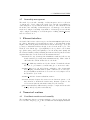
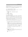
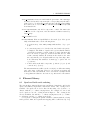
quads; and trilinear, triquadratic, and tricubic bricks. The ordering is nonstandard. For quads, the nodes are listed in increasing order by their coordinates, with the y coordinate varying fastest. For example, for 4-node and
9-node quads, we use the ordering shown in Figure 1. The ordering in the
3D case is similar, but with the z coordinate varying fastest, the y coordinate
second-fastest, and the x coordinate most slowly.
So long as the ordering in the spatial domain is consistent with the ordering
in the parent domain, the isoparametric mapping will be well-behaved (so long
12
6
2
1
4
3
ELEMENT LIBRARY
3
6
9
2
5
8
1
4
7
Figure 1: Node ordering for 4-node and 9-node quads
as element distortion is not too great). The add block commands described in
Section 2.3 produce node orderings which are consistent with our convention.
The primary advantage of the node ordering we have chosen is that it becomes trivial to write loops to construct 2D and 3D tensor product shape functions out of simple 1D Lagrangian shape functions. Also, it becomes simple to
write the loops used to convert a mesh of higher order elements into four-node
quads or eight-node bricks for visualization (see Section 5.1).
Development note: Currently, the number of Gauss points used by the element library is fixed at compile time. It might be wise to allow the user to
change that.
6.2
PML elements
Perfectly matched layers (PMLs) are layers subject to complex-value coordinate
transformations which are used to mimic the effect of an infinite or semi-infinite
medium. PMLs fit naturally into a finite element framework, but to implement
them, we need some way to describe the exact form of the coordinate transformation. The PMLElement class is derived from the standard Element class (see
Section 3), and defines two additional methods for describing the coordinatestretching function used in a PML:
set stretch(L,s) Use a Lua function to describe the coordinate transformation. The function is stored in the Lua interpreter L at stack index s.
It is not applied immediately, but only when the stretching function is
actually evaluated; consequently, the Lua interpreter should not be destroyed before the last call to the element methods for computing local
residuals and tangents.
The coordinate stretching function in 2D should have the form
function stretch(x,y)
-- Compute stretching parameters sx and sy
13
6
ELEMENT LIBRARY
return sx, sy
end
If no stretch values are returned, they are assumed to be zero. The PML
element should stretch the x and y coordinates by (1 − isx ) and (1 − isy ),
respectively. The 3D case is handled similarly.
The stretching function is only ever evaluated at node positions.
set stretch(stretch,ndm,nen) Use the ndm-by-nen array stretch to look
up the stretch function values at the nodes.
If there are no calls to either form of set stretch, the PML element does not
stretch the spatial coordinate at all, and so the element behaves exactly like an
ordinary (non-PML) element.
6.3
Laplace elements
The PMLScalar2d, PMLScalar3d, and PMLScalarAxis classes implement scalar
wave equation elements with an optional PML. If no coordinate stretching is
defined, the elements will generate standard (real) mass and stiffness matrices.
PMLScalar2d(kappa,rho,nen) Creates an isotropic 2D scalar wave equation element with material property κ and mass density ρ. The number
of element nodes nen must be 4 (bilinear), 9 (biquadratic), or 16 (bicubic).
PMLScalar2d(D,rho,nen) Creates a 2D anisotropic element with a 2-by-2
property matrix D. Other than the material properties, this constructor
is identical to the previous one.
PMLScalarAxis(kappa,rho,nen) Creates an isotropic axisymmetric scalar
wave equation element with material property κ and mass density ρ. The
number of element nodes nen must be 4 (bilinear), 9 (biquadratic), or 16
(bicubic).
PMLElasticAxis(D,rho,nen) Creates a 2D anisotropic element with a 2by-2 property matrix D. Other than the material properties, this constructor is identical to the previous one.
PMLScalar3d(kappa,rho,nen) Creates an isotropic 3D scalar wave equation element with material property κ and mass density ρ. The number
of element nodes nen must be 8 (trilinear), 27 (triquadratic), or 64 (tricubic).
PMLScalar3d(D,rho,nen) Creates a 3D anisotropic element with a 3-by-3
property matrix D. Other than the material properties, this constructor
is identical to the previous one.
14
7
6.4
LUA INTERFACES
Elastic elements
The PMLElastic2d, PMLElastic3d, and PMLElasticAxis classes implement
elasticity elements with an optional PML transformation. The classes provides
the following constructors:
PMLElastic2d(E,nu,rho,plane type,nen) Creates a plane strain (plane type
= 0) or plane stress (plane type = 1) isotropic elasticity element with
Young’s modulus E, Poisson ratio nu, and mass density rho. The number of element nodes nen must be 4 (bilinear), 9 (biquadratic), or 16
(bicubic).
PMLElastic2d(D,rho,nen) Creates a 2D element with a 3-by-3 elastic property matrix D. Other than the elastic properties, this constructor is identical to the previous one.
PMLElasticAxis(E,nu,rho,nen) Creates an isotropic axisymmetric elasticity element with Young’s modulus E, Poisson ratio nu, and mass density rho. The number of element nodes nen must be 4 (bilinear), 9
(biquadratic), or 16 (bicubic).
PMLElasticAxis(D,rho,nen) Creates an element with a 4-by-4 elastic property matrix D. Other than the elastic properties, this constructor is identical to the previous one.
PMLElastic3d(E,nu,rho,nen) Creates an isotropic 3D elasticity element
with Young’s modulus E, Poisson ratio nu, and mass density rho. The
number of element nodes nen must be 8 (trilinear), 27 (triquadratic), or
64 (tricubic).
PMLElastic3d(D,rho,nen) Creates an element with a 6-by-6 elastic property matrix D. Other than the elastic properties, this constructor is identical to the previous one.
7
Lua interfaces
Lua is a language invented at PUC-Rio in Brazil. The Lua language and standard libraries are very lightweight, enough so that the complete Lua interpreter
library can be statically linked into the HiQLab executable without much space
penalty. Lua is well-suited as a scripting language for a finite element code for
the following reasons:
• The syntax is very simple, and is reminiscent of Pascal. The complete
EBNF grammar for the language fits on one page.
• The language supports dynamic typing, first-class functions, and other
features which are useful in concisely describing meshes and numerical
algorithms.
15
7
LUA INTERFACES
• The interpreter uses a reasonably fast stack-based bytecode machine. The
overhead of calling a function at every node in a mesh, for example, is
not too onerous. (This is a large part of why Lua is popular for game
scripting.)
• The interpreter provides native support for C/C++ user types.
• Lua was designed as an extension language (as compared to some languages which are effective as steering languages or as extensible languages,
but which are difficult to force into secondary modules). It is possible to
instantiate multiple interpreters simultaneously; calls to and from C++
are simple and fast; and it is very simple to call Lua from within a MATLAB MEX file.
• Lua is licensed under a variant of the MIT license, and can be used for
both commercial and academic purposes at no cost.
HiQLab uses version 5 of the Lua language system. The Lua interpreter and
libraries are included in the tools subdirectory of the HiQLab build tree.
7.1
Automatic binding
tolua is a tool to automatically bind Lua to C or C++. tolua takes a cleaned
header file as input, and generates code to automatically add bindings to the
listed C/C++ functions and data objects. Type checking is performed automatically.
Most of tolua’s functionality is described in the tolua manual (though
the manual has not been updated since version 3.2). However, one piece of
functionality is not well described in the user manual: the ability to pass native
Lua objects to C/C++ codes. For example, the cleaned header file used to bind
the PMLElement class methods to Lua contains the line
void set_stretch(lua_State* L, lua_Object func);
which corresponds to the C++ function
void set_stretch(lua_State* L, int func);
With this binding, Lua can call set stretch as
mesh:set_stretch(stretchfun)
and the C++ function will automatically receive a pointer to the Lua interpreter
together with the Lua stack location of the function object. Thus, tolua makes
it easy to pass a Lua callback to a C++ function.
One other feature makes Lua callbacks simple to implement: the registry
table. Since a Lua function does not correspond to any simple C++ object, we
cannot just store a pointer to the Lua function in a field in the C++ class. The
most obvious way to store the callback would be to store its name as a string;
16
7
LUA INTERFACES
this can cause problems, though, if the user would like to define a transformation
using an anonymous (lambda) function – a surprisingly useful thing to do – or
if the user would like to use a function which is not defined in the global scope.
However, Lua provides a registry table which is accessible only from compiled
code. So to store a Lua callback, we write a registry table entry keyed by the
this pointer of the corresponding C++ object.
See the PMLElement implementation for a simple example of the type of
callback described above.
7.2
Modifying automatically bound interfaces
When tolua creates binding code for a class, it builds a table with the same
name as the class. This table is attached to each bound instance of the class
as a Lua metatable – that is, the Lua interpreter will check the class table for
fields that it cannot find in the instance table (such as methods). This lookup is
almost identical to vtable lookup for virtual functions in C++. A natural way to
add methods to the Lua version of the class is to add functions to this class table.
These new methods can replace methods for which the automatically generated
binding does not naturally fit, or add new methods which take advantage of Lua
features. For example, the binding of the QArray matrix class in Lua contains
the Lua code
function QArray:size()
return self:m(), self:n()
end
which adds a size method with two return values to the Lua code.
7.3
Error handling in Lua callbacks
Lua uses a setjmp / longjmp-based error handling scheme internally. A C function calling into Lua has two options for handling errors: it can use lua call,
in which case any errors generated are thrown by longjmp up the stack to be
caught by the next available handler; or it can use lua pcall, which returns a
status code and, in case of an error, pushes a string describing the error onto the
Lua stack. The lua pcall function also allows an error handler to be defined.
The callbacks in HiQLab use a small wrapper around lua pcall, called
lua pcall2. lua pcall2 acts the same as lua pcall except when an error
occurs. If there is an error, lua pcall calls the Lua function ALERT (if it is
defined) to show the message; otherwise, it prints the message to stderr using
the C fprintf function. In either case, the error message string is removed
from the stack before control is returned to lua pcall2’s caller.
As a matter of policy, HiQLab code that uses callbacks should make every
effort to provide reasonable default behaviors (including a diagnostic message)
if the user-defined Lua code does something silly.
17
7
7.4
LUA INTERFACES
Using Lua with MATLAB
When Lua is used from within the MATLAB environment, it should not print
to stderr and stdout, since those streams are not redirected to the MATLAB
GUI window. The luamex package in the MATLAB interface code, which is
automatically included when a Lua interpreter is instantiated from MATLAB,
re-defines print and the ALERT function (see Section 7.3) in terms of MATLAB’s mexPrintf function.
The functions in the luasupport package allow MATLAB dense or sparse
matrices to be passed back and forth to Lua. MATLAB dense arrays are converted to and from QArray objects, and MATLAB sparse matrices are converted
to and from CSCMatrix objects.
7.5
Automatically bound interfaces
The Lua interface includes bindings to the following classes and functions described previously:
The mesh object
The element library
The CoordMatrix assembler
The CSCMatrix class
The DXFile class
The mesh version of compute eigs
Development note: The compute eigs binding, like compute eigs as a whole,
is something of a hack. The right way to handle this is probably to bind
ARPACK directly to Lua a la MATLAB’s eigs. However, this “right way”
would probably also have at least a few days programming cost.
7.6
Transformed block generation in Lua
The Lua binding of the Mesh class contains two additional block generators
beyond those in the C++ binding:
add block transform(m,n,p,order,func) Creates a 3D (or 2D if p is omitted) quad block with node positions on [−1, 1]n and transforms them
using the specified function.
add block transform(m,n,p,order,pts) Creates a 3D (or 2D if p is omitted) quad block with node positions on [−1, 1]n and transforms them
using an isoparametric mapping with points specified in the pts array.
For example, for pts = {0,0, 0,1, 1,0, 1,1}, we would get a mesh
for [0, 1]2 .
18
7
7.7
LUA INTERFACES
Dense matrices in Lua
tolua wraps arrays whose sizes can be easily computed, but it passes those
arrays through Lua tables. Lua tables are an inefficient way to store long vectors,
so we introduce a small container class QArray to manipulate array data more
efficiently.
QArray objects may either manage their own storage, or they can point to
another array for their storage. The latter mode is useful for functions like eigs,
which require another program to manipulate some part of a workspace array.
QArrays can be real, complex, or complex stored in two parts, and they can be
accessed using either zero-based or one-based indexing. These options are set
when the QArray is constructed, and can be retrieved later; they are controlled
by the following variables:
m
Number of rows
n
Number of columns
type Type of matrix data
type == 0 Real matrix
type == 1 Complex data stored in one array
type == 2 Complex data stored in two arrays
base First index (0 for C-style, 1 for Fortran/MATLAB-style)
The QArray class provides the following methods:
set(i,j,xr,xi=0) Set real and imaginary parts of the ij entry
get(i,j)
Get the real part of the ij entry
geti(i,j)
Get the imaginary part of the ij entry
Development note: Should there be separate setr and seti methods so that
it’s possible to write just the real component without zeroing out the imaginary
component?
Development note: Should check to make sure the user can’t chain together
assignments in such a way as to refer to an allocated block after it has been
deleted.
7.8
Sparse matrices in Lua
The Lua CSCMatrix binding is similar to the C++ class, but differs in that it
uses QArray objects to pass vectors. The methods provided in the Lua binding
are
n()
Return the matrix size
19
8
MATLAB INTERFACES
apply(x,y) Compute y = Ax
solve(x,b) Solve Ax = b
apply(x)
Compute y = Ax
solve(b)
Solve Ax = b
8
MATLAB interfaces
8.1
Automatic binding
The matwrap program is a Perl program which generates MATLAB wrappers
based on C/C++ header files. The project was inspired by the SWIG wrapper generator, with extensions to make it easier to interface to matrix-oriented
languages. Beside MATLAB, matwrap also automatically generates output for
Octave and Tela.
We have made a number of modifications to matwrap:
1. Package files
The original version of matwrap accepts only header files, which it expects
to be valid C/C++ header files which can be included in the generated
wrapper. However, the matwrap parser is not sophisticated, and it deals
poorly with templates, preprocessor macros, inline functions, and various
other syntactically complicated things. We therefore introduce package
files (pkg extension), cleaned header files analogous to those used in tolua.
matwrap will only use the package file to generate wrappers; it will not
attempt to include the file as a header file for the wrapper code.
2. Inlined sources
To support package files, we need some way to include the actual headers
in the wrapper file. We extended matwrap so that lines in a package
file which begin with a dollar sign are included near the beginning of the
wrapper code. For example, in foo.pkg, we might have the line $#include
‘‘foo.h’’.
3. Inlined function files
Package files may contain MATLAB function definitions inline, delimited
by $[ and $]. matwrap generates a MATLAB M-file named based on the
first function definition in the bracketed text.
4. Direct manipulation of MATLAB objects
It is sometimes useful to directly work with MATLAB objects that have no
standard C++ counterparts: sparse matrices are a good example. Package
files can refer to m Objects to pass unprocessed MATLAB mxArray values
to or from a wrapped function. Like wrappers involving strings, wrappers
that involve mutable m Objects cannot be vectorized.
20
8
MATLAB INTERFACES
Method wrappers generated for MATLAB use a full name and an explicit
this pointer. For example, to call method foo() of class Bar, a MATLAB user
would write
Bar_foo(barobj);
matwrap does not deal well with methods which have the same name and differ
only in type signature. When this problem occurs, we currently write an additional layer of thin C++ wrappers which really serve only to give the function
a new name and thereby break the aliasing effect.
matwrap is installed in the HiQLab tools subdirectory.
Development note: Ideally, we would like to use MATLAB’s OO facilities to
save explicitly typing the class name on every method invocation. This would
mostly involve mechanically re-writing generated functions, with one exception:
we would either need to provide additional code for explicit casting between
compatible types, or we would need to let MATLAB know about the inheritance
relationships in the C++ code. Since matwrap generates wrappers that know
about those relationships, the right way to deal with this might again be to
rewrite part of matwrap. The current – very slick – scheme is to represent
objects as pointers, in which the real part contains the actual pointer data and
the imaginary part contains a type code.
Development note: It’s too easy to create leaks in MATLAB. Should there
be a registry for mesh objects so we can say “clear all allocated meshes” and
have the right thing happen? What about error conditions?
8.2
Automatically bound interfaces
The same interfaces that are automatically bound to Lua are also automatically bound to MATLAB. In addition, several methods are defined which allow
MATLAB to manipulate a Lua interpreter:
Lua open Return a pointer to a new Lua interpreter L
Lua close(L) Close the Lua interpreter
Lua dofile(L,filename) Execute a Lua file
Lua set mesh(L,name,mesh) Assign a mesh object to a Lua global
Lua get mesh(L,name) Retrieve a mesh object from a Lua global
Lua set string(L,name,s) Assign a string to a Lua global
Lua set double(L,name,x) Assign a number to a Lua global
The Lua object interface is used in the MATLAB Mesh load function:
21
8
MATLAB INTERFACES
Mesh load(filename,p) Creates a Lua interpreter and executes the named
file in order to generate a mesh object (which is returned). The mesh
should be named “mesh”; if such an object is undefined on output,
Mesh load returns an error message. Before executing the named file,
Mesh load copies the entries of the structure p, which may only be strings
or doubles, into the Lua global state; in this way, it is possible to vary
mesh parameters from MATLAB.
8.3
Eigencomputations
The MATLAB sparse eigensolver routine eigs is actually an interface to ARPACK
(see Section 4.3). We express all frequencies in radians/s rather than Hertz.
We provide one function to compute complex frequencies and associated mode
shapes for PML eigenvalue problems:
pml mode(M,K,w0,nmodes,opt) Find the requested number of modes closest in frequency to w0. Return an array of mode shapes, a vector of
complex frequencies, and a vector of Q values. Options are
use matlab Use MATLAB’s eigs rather than ARPACK? (default: false)
use umfpack Use UMFPACK with MATLAB eigs, if present? (default:
true)
disp
Verbosity level? (default: 0)
8.4
Energy flux computations
The compute flux2d and compute flux3d compute time-averaged energy flux
vector fields. These routines are themselves in flux.
Development note: The interface to assemble the list of stresses at Gauss
nodes changed since I wrote the compute flux functions. These functions need
to be brought up to date.
8.5
Model reduction
There is currently one model reduction routine in the MATLAB support files
for HiQLab. As before, all frequencies are expressed in radians/s rather than
Hz.
rom arnoldi(M,K,l,b,kk,w0,opt) Takes kk steps of shift-and-invert Arnoldi
to form a basis for the Krylov subspace Kk (K − (2πω0 )2 M )−1 M, b in
order to form a reduced system to estimate the system transfer function.
Returns reduced matrices Mk , Kk , lk , and bk , along with the projection
basis Vk . If opt.realbasis is set to true (default is false), then the projection will use a real basis for the span of [Re(Vk ), Im(Vk )]. To do this,
the matrix [Re(Vk ), Im(Vk )] will be orthonormalized using an SVD, and
vectors corresponding to values less than opt.realtol (default 10−8 )
will be dropped.
22
8
8.6
MATLAB INTERFACES
Plotting
There are several plotting routines for viewing the behavior of 2D meshes:
plotmesh(mesh,opt) Plots a given mesh. Options are
anchors Marker for nodes with displacement BC (default: ’g+’)
forces Marker for nodes with force BC (default: ’r+’)
deform Deform mesh according to first to fields of u? (default: false)
clf Clear the figure before display? (default: true)
plotcycle2d(mesh,s,opt) Plot an animation of the motion of the mesh.
The amplitude of motion is scaled by the factor s (which defaults to one
if it is not provided). The frames can be written to disk as a sequence
of PNG files to make a movie later. The following options can be set
through the opt structure
framepng Format string for movie frame files (default: [])
nframes
Number of frames to be plotted (default: 32)
fpcycle
Frames per cycle (default: 16)
startf
Start frame number (default: 1)
fpause
Pause between re-plotting frames (default: 0.25)
cscale
Color all fields on the same scale? (default: false)
ufields
Fields to use for displacement (default: [1 2])
ufields
Fields to use for coloring (default: [1 2])
axequal
Use equal axes in plots? (default: false)
subplot
Subplot setup (default: [length(cfields), 1])
The element array defined inside the mesh object cannot immediately be used
inside the plot routines. The following utility function rearranges the connectivity array into a form that plays nicely with MATLAB’s plotting routines (see
also Section 5.1):
plotelt2d(e) Returns a “flattened” version of the element connectivity
array e for use with the plotting routine. The flattened element array
will contain the same number of entries as elements in the bilinear case,
but biquadratic and bicubic elements will be converted into lists of four
or nine 4-node panels. The rearranged panels follow a counterclockwise
node ordering.
In addition, there is a function for viewing Bode plots:
plot bode(freq,H,opt) Plots a Bode plot. H is the transfer function evaluated at frequency points freq. The option structure opt may contain
the following options:
23
8
MATLAB INTERFACES
usehz
Assume freq is in Hz (default: false)
logf
Use a log scale on the frequency axis (default: false)
magnitude Plot magnitude only (default: false)
visualQ
Visually compute Q for the highest peak (default: false)
lstyle
Set the line style for the plot (default: ’b’)
For example, to plot a reduced model Bode plot on top of an exact Bode
plot, we might use the following code:
figure(1);
opt.logf =
opt.lstyle
opt.lstyle
hold off
hold on
1;
= ’b’ ; plot_bode(freq_full, H_full, opt);
= ’r:’; plot_bode(freq_rom, H_rom, opt);
It is also possible to simultaneously show a deformed mesh and a Bode plot with
a marker indicating the excitation frequency.
plotmesh bode(mesh,f,H,fcurrent,opt) Plot the deformed mesh and create a Bode plot. The opt field is passed through to plotmesh.
24