Download MaxFilter 2.0 Manual

MaxFilter
User’s Guide
Software version 2.0
October 2006
Copyright © 2006 Elekta Neuromag Oy, Helsinki, Finland.
Elekta assumes no liability for use of this document if any unauthorized changes to the content or format have been
made.
Every care has been taken to ensure the accuracy of the information in this document. However, Elekta assumes no
responsibility or liability for errors, inaccuracies, or omissions that may appear in this document.
Elekta reserves the right to change the product without further notice to improve reliability, function or design.
This document is provided without warranty of any kind, either implied or expressed, including, but not limited to,
the implied warranties of merchantability and fitness for a particular purpose.
Elekta Neuromag, MaxFilter and MaxShield are trademarks of Elekta.
This product is protected by the following issued or pending patents:
US2006031038 (Signal Space Separation)
US6876196 (Head position determination)
WO2005067789 (DC fields)
WO2005078467 (MaxShield)
FI20050445 (MaxST)
Printing History
Neuromag p/n
Software
Date
5th edition
NM21492A-D
1.1
January 2005
1st edition
NM21993A
2.0
October 2006
NM21993A
Contents
Chapter 1 Introduction
1.1
1.2
1.3
1.4
5
Overview . . . . . . . . . . . . . . . . . . . . . . . . . . . . . . . . . . . . . . . . . .
Maxwell filtering . . . . . . . . . . . . . . . . . . . . . . . . . . . . . . . . . . . .
Software functionality . . . . . . . . . . . . . . . . . . . . . . . . . . . . . . . .
Software safety . . . . . . . . . . . . . . . . . . . . . . . . . . . . . . . . . . . . .
Chapter 2 Using MaxFilter
2.1 Background . . . . . . . . . . . . . . . . . . . . . . . . . . . . . . . . . . . . . . .
2.2 Launching the program . . . . . . . . . . . . . . . . . . . . . . . . . . . . .
Graphical User Interface . . . . . . . . . . . . . . . . . . . . . . . . . . . . . .
Command line . . . . . . . . . . . . . . . . . . . . . . . . . . . . . . . . . . . . . .
2.3 GUI main window . . . . . . . . . . . . . . . . . . . . . . . . . . . . . . . . . .
2.4 Menus . . . . . . . . . . . . . . . . . . . . . . . . . . . . . . . . . . . . . . . . . . . .
File . . . . . . . . . . . . . . . . . . . . . . . . . . . . . . . . . . . . . . . . . . . . . .
Filter . . . . . . . . . . . . . . . . . . . . . . . . . . . . . . . . . . . . . . . . . . . . .
Move . . . . . . . . . . . . . . . . . . . . . . . . . . . . . . . . . . . . . . . . . . . . .
Averager . . . . . . . . . . . . . . . . . . . . . . . . . . . . . . . . . . . . . . . . . .
Help . . . . . . . . . . . . . . . . . . . . . . . . . . . . . . . . . . . . . . . . . . . . . .
2.5 Loading data . . . . . . . . . . . . . . . . . . . . . . . . . . . . . . . . . . . . . .
2.6 Output options . . . . . . . . . . . . . . . . . . . . . . . . . . . . . . . . . . . .
Filename . . . . . . . . . . . . . . . . . . . . . . . . . . . . . . . . . . . . . . . . . .
Data packing . . . . . . . . . . . . . . . . . . . . . . . . . . . . . . . . . . . . . . .
Ignoring warnings . . . . . . . . . . . . . . . . . . . . . . . . . . . . . . . . . . .
Processing history . . . . . . . . . . . . . . . . . . . . . . . . . . . . . . . . . . .
2.7 Logging the output . . . . . . . . . . . . . . . . . . . . . . . . . . . . . . . . .
Chapter 3 MaxFilter parameters
3.1 Expansion origin . . . . . . . . . . . . . . . . . . . . . . . . . . . . . . . . . . .
3.2 Harmonic basis functions . . . . . . . . . . . . . . . . . . . . . . . . . . .
3.3 Bad channels settings . . . . . . . . . . . . . . . . . . . . . . . . . . . . . .
Autobad . . . . . . . . . . . . . . . . . . . . . . . . . . . . . . . . . . . . . . . . . . .
Evoked data . . . . . . . . . . . . . . . . . . . . . . . . . . . . . . . . . . . . . . .
Raw data . . . . . . . . . . . . . . . . . . . . . . . . . . . . . . . . . . . . . . . . . .
Sensor artifacts . . . . . . . . . . . . . . . . . . . . . . . . . . . . . . . . . . . . .
3.4 MaxST settings . . . . . . . . . . . . . . . . . . . . . . . . . . . . . . . . . . . .
3.5 MEG sensors . . . . . . . . . . . . . . . . . . . . . . . . . . . . . . . . . . . . . .
Sensor types . . . . . . . . . . . . . . . . . . . . . . . . . . . . . . . . . . . . . . .
Sensor noises . . . . . . . . . . . . . . . . . . . . . . . . . . . . . . . . . . . . . .
Calibration adjustment and cross-talk correction . . . . . . . . . . .
5
6
8
9
11
11
12
12
12
13
14
14
14
15
15
15
16
17
17
18
18
18
20
21
21
22
24
24
25
25
26
27
29
29
29
29
i
Changing the fine-calibration and cross-talk correction . . . . . . . 30
Reconstruction of sensor signals . . . . . . . . . . . . . . . . . . . . . . . . 31
3.6 Default parameters . . . . . . . . . . . . . . . . . . . . . . . . . . . . . . . . . 32
Chapter 4 MaxMove parameters
4.1
4.2
4.3
4.4
4.5
4.6
Data transformation . . . . . . . . . . . . . . . . . . . . . . . . . . . . . . . .
Head position tracking . . . . . . . . . . . . . . . . . . . . . . . . . . . . . .
Head position estimation . . . . . . . . . . . . . . . . . . . . . . . . . . . .
Movement compensation . . . . . . . . . . . . . . . . . . . . . . . . . . . .
Low-pass filtering . . . . . . . . . . . . . . . . . . . . . . . . . . . . . . . . . .
Default parameters . . . . . . . . . . . . . . . . . . . . . . . . . . . . . . . . .
Chapter 5 MaxAve parameters
5.1
5.2
5.3
5.4
Background . . . . . . . . . . . . . . . . . . . . . . . . . . . . . . . . . . . . . . .
Launching the program . . . . . . . . . . . . . . . . . . . . . . . . . . . . .
Selecting files . . . . . . . . . . . . . . . . . . . . . . . . . . . . . . . . . . . . .
Averaging parameters . . . . . . . . . . . . . . . . . . . . . . . . . . . . . . .
Appendix A Maxwell filtering in a nutshell
A.1
A.2
A.3
A.4
Signal space separation . . . . . . . . . . . . . . . . . . . . . . . . . . . . .
Harmonic amplitudes . . . . . . . . . . . . . . . . . . . . . . . . . . . . . . .
Pseudoinverse . . . . . . . . . . . . . . . . . . . . . . . . . . . . . . . . . . . . .
Optimization of virtual channel selection . . . . . . . . . . . . . . .
Appendix B Elekta Neuromag MEG sensors
33
33
35
37
38
39
40
41
41
41
43
43
45
45
46
47
47
49
B.1 Sensor types . . . . . . . . . . . . . . . . . . . . . . . . . . . . . . . . . . . . . . 49
B.2 Scaling between magnetometers and gradiometers . . . . . . 50
B.3 Manipulation of sensor types . . . . . . . . . . . . . . . . . . . . . . . . . 51
Appendix C Temporal subspace projection
53
Appendix D Head position estimation
55
D.1
D.2
D.3
D.4
ii
HPI signals . . . . . . . . . . . . . . . . . . . . . . . . . . . . . . . . . . . . . . . .
Coordinate matching . . . . . . . . . . . . . . . . . . . . . . . . . . . . . . . .
HPI channels . . . . . . . . . . . . . . . . . . . . . . . . . . . . . . . . . . . . . .
Head position file format . . . . . . . . . . . . . . . . . . . . . . . . . . . .
55
56
57
57
Appendix E Command-line arguments
59
Appendix F Revision history
63
1
CHAPTER 1
Introduction
1.1 Overview
This User’s Guide gives detailed explanation of the Elekta Neuromag
MaxFilter 2.0 software for MEG data analysis.
MaxFilter is intended to be used with Elekta Neuromag MEG products in
suppressing magnetic interferences coming from inside and outside of the
sensor array, in reducing measurement artifacts, in transforming data
between different head positions, and in compensating disturbances due to
head movements.
This Chapter presents a general overview and main functionalities of the
software. Chapters 2-5 describe how to start the program, and how to control the functionality and parameters. Mathematical background and some
further information are included in the Appendices.
NM21993A
2006-10-31
5
1
Introduction
1.2 Maxwell filtering
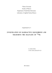
Signal Space Separation is a method that utilizes the fundamental properties of electromagnetic fields and harmonic function expansions in separating the measured MEG data into three components (Figure 1.1):
b in :
b out :
n:
The brain signals originating inside of the sensor array
(space S in ).
External disturbances arising outside of the sensor array
(space S out ).
Noise and artifacts generated by the sensors and sources of
interference located very close to the sensors (space S T ).
Sout
n
ST
Sin
Figure 1.1 The geometry in Maxwell filtering. One hypothetical spherical
shell inside of the sensor array encloses the subject’s brain, and another
one encloses all MEG sensors. The radii of the shells are determined,
respectively, as the smallest and largest distances from the origin to the
sensor locations.
The disturbing magnetic interferences are suppressed by omitting the harmonic function components corresponding to unduly high spatial frequencies, by neglecting the S out -space component b out , and by reducing the
S T -space component n .
Since the method is based directly on Maxwell’s equations, the operation
can be called Maxwell filtering; hence the name MaxFilter.
The basic Maxwell filtering operation can be regarded as spatial filtering,
because separation of b in and b out is done on the basis of the spatial patterns and is independent of time. Spatial separation can suppress only
external interferences emanating from space S out , such as electromagnetic pollution due to power lines, radio communication, traffic, elevators
etc. External interference can also arise in the patient. For instance, normal cardiac and muscular activation cause fields detectable by MEG sen-
6
2006-10-31
NM21993A
Introduction
1
sors, and any pieces of magnetized material in/on the body may cause
very large disturbances.
Identification and suppression of the S T -space components require additional knowledge of the temporal dynamics. Spatio-temporal extension to
Maxwell filtering, called MaxST, widens significantly the software shielding capability of MaxFilter, because MaxST can suppress also internal
interferences that arise in the S T -space or very close to it. Such internal
interferences can be caused, for example, by magnetized pieces in/on the
subject's head (such as dental work, braces, or magnetized left-overs in
burr-holes), or by pacemakers or stimulators attached to the patient.
Maxwell filtering inherently transforms measured MEG signals into virtual channels in terms of harmonic function amplitudes. Because the virtual channels are independent of the device, they offer a straightforward
method for estimating corresponding MEG signals in other sensor arrays.
This function called MaxMove provides an elegant way to transfer MEG
signals between different head positions and to compensate for disturbances caused by head movements during recordings.
The mathematical basis of Maxwell filtering is described briefly in
Appendix A. The Signal Space Separation algorithms and their applications are discussed in detail in:
1. S. Taulu, M. Kajola, and J. Simola. Suppression of interference and
artifacts by the signal space separation method. Brain Topography
16(4), 269-275, 2004.
2. S. Taulu, and M. Kajola. Presentation of electromagnetic multichannel
data: the signal space separation method. Journal of Applied Physics,
97(12), 124905, June 2005.
3. S. Taulu, J. Simola, and M. Kajola. Applications of the signal space
separation method. IEEE Transactions on Signal Processing, 53(9),
3359-3372, 2005.
4. S. Taulu, and J. Simola. Spatiotemporal signal space separation method
for rejecting nearby interference in MEG measurements. Physics in
Medicine and Biology, 51, 1759-1768, 2006.
NM21993A
2006-10-31
7
1
Introduction
1.3 Software functionality
MaxFilter 2.0 software provides three separate programs:
MaxFilter
The main application for doing Maxwell filtering called from
a command line. This program includes also MaxST and MaxMove functions.
MaxAve
Off-line version of the on-line averager, provided for convenient re-averaging of raw data before or after Maxwell filtering.
MaxFilter_GUI
Graphical user interface program which collects the input
arguments, and then starts MaxFilter or MaxAve as a subprocess. Information of the data processing is displayed on the
main display and in a log window.
The main functions of MaxFilter are:
Software shielding
By subtracting the component b out from measured signals b ,
the program performs software shielding on the measured
MEG data.
Automated detection of bad channels
By comparing the reconstructed sum b in + b out with measured signals b , the program can automatically detect if there
are MEG channels with bad data that need to be excluded
from Maxwell filtering.
Spatio-temporal suppression of S T -space artifacts
By subtracting the reconstructed waveforms b in ( t ) + b out ( t )
from measured signals b ( t ) , the program can identify and
suppress artifact waveforms which arise in the S T -space.
Transformation of MEG data between different head positions
By transforming the component b in into harmonic amplitudes
(i.e. virtual channels), MEG signals in a different head position can be estimated easily.
Compensation of disturbances caused by head movements
By extracting head position indicator (HPI) signals applied
continuosly during a measurement, the data transformation
capability is utilized to estimate the corresponding MEG signals in a static reference head position.
8
2006-10-31
NM21993A
Introduction
1
1.4 Software safety
MaxFilter is easy to apply and the default settings provide good results in
most cases. Maxwell filtering as implemented in this program is an irreversible operation. The expansion corresponding to the space outside of
the sensor array ( b out ) is discarded before saving the result. In addition,
MaxST projects out artifact waveforms identified in the sensor space.
Note: The original recording cannot be reconstructed from the result FIFF
file. Therefore, it is very important to keep also the original data files on
suitable backup media after applying MaxFilter.
This manual contains important hazard information which must be read,
understood and observed by all users. General limitations of the program
are included in the following Chapters. For your convenience all warnings
that appear in the manual are presented below.
NM21993A
!
Warning: It is important that the user inspects both the input and the output data visually to judge the quality of the Maxwell filtering result.
!
Warning: If the fine-calibration and cross-talk correction data are not
available, the performance of Maxwell filtering may not be as good as
with the fine-calibrated system.
!
Warning: Special care should be taken to ensure that right fine-calibration data are used for imported or old data for which the default calibration does not apply.
!
Warning: If the threshold of the automated bad channel detection is too
small, the program may classify good channels as bads, and if it is too
high, some bad channels may remain undetected.
!
Warning: When transforming data from one head position into another
special care should be taken to ensure that both head positions are accurately defined in respect to the sensor array.
!
Warning: Head position calculation errors affect the data quality after
movement compensation. The user must inspect the head position fitting
error and goodness before data analysis.
!
Warning: If MaxShield™ was applied in the input file, the user must not
perform data analysis on MaxFilter output files obtained with the options
-nosss or -ctc only.
2006-10-31
9
1
10
Introduction
2006-10-31
NM21993A
2
CHAPTER 2
Using MaxFilter
2.1 Background
MaxFilter can be applied to a FIFF-file with raw data or averaged MEG
measurement results. The parameters needed in calculations are set to
well-defined initial values, separately for Elekta Neuromag®, Neuromag
System, and Neuromag-122 data. The default settings are listed in Sections 3.6 and 4.6, and you can run the program without changing these
values. However, sometimes it may be useful to tune the details of the
Maxwell filtering operation.
In brief, you can change the dimensions of the internal and external multipole bases and the origin of the expansions. Optionally, you can manually
identify and set bad channels that are not taken into account in the reconstruction. In cases where the source of interference is located inside or
very close to the sensor array, it is recommended to use the spatio-temporal Maxwell filtering, MaxST. In addition, you can transfer data between
different head positions, and compensate disturbances due to head movements using MaxMove.
!
NM21993A
Warning: It is important that the user inspects both the input and the output data visually to judge the quality of the Maxwell filtering result.
2006-10-31
11
2
Using MaxFilter
2.2 Launching the program
2.2.1 Graphical User Interface
The graphical user interface, GUI, is a program that collects the input
parameters of MaxFilter or MaxAve, and then runs the command-line program as a subprocess. You can monitor the execution on a log window
(Section 2.7). The GUI can be launched in
HP-UX 11:
Click the Neuromag toolbox icon labeled as MaxFilter.
Linux:
Select the menu Applications –> Other, click icon MaxFilter.
Command line:
/neuro/bin/vue/maxfilter_gui.
Upon launching the program checks available licenses, and displays a
welcome logo (Figure 2.1). Click Hide to close the window.
Figure 2.1 MaxFilter welcome window.
2.2.2 Command line
Alternatively, you can start MaxFilter from a command line as
/neuro/bin/util/maxfilter -f input_file.fif
[options]
If no arguments are given, the program gives just a brief message:
usage: maxfilter -f <infile> [options]
’maxfilter -help’ shows available options.
A comprehensive list of the options is given in Appendix E.
12
2006-10-31
NM21993A
Using MaxFilter
2
2.3 GUI main window
The main window consists of the following areas:
1.
2.
3.
4.
5.
Figure 2.2 MaxFilter GUI main window.
1.
2.
3.
4.
5.
The menubar.
A text area for showing current parameter values.
Drawing area which shows the head position estimation parameters.
Display area for showing the processing status.
A message text label at the bottom of the window.
The menus and controls are described in the following sections.
When you have defined the input and output filenames and modified the
parameters, press Execute to start Maxwell filtering. The progress scale
bar indicates the number of processed buffers. You can press STOP to
cancel processing. Then you can modify the parameters and try again
(press Execute).
The labels next to STOP button indicate the number of warnings and
errors reported by MaxFilter. During execution, the background colour of
these labels is green. If there are warnings, background of the label
warnings changes to red and the label reports the number of warnings.
If MaxFilter is terminated due to a fatal error, background of the label
errors turns to red.
NM21993A
2006-10-31
13
2
Using MaxFilter
The scale bar and the text label at the bottom indicate the status of the
Maxwell filtering operation. You can view more detailed information of
the MaxFilter output and warnings by selecting Show log from the File
menu.
When you start MaxMove processing (see Chapter 4), the program starts
head position estimation. Estimated head postion parameters are drawn in
the plotting area of the main window:
•
•
•
•
•
white curve: fitting error
red curve: goodness of fit
green curve: translational movement velocity
blue curve: rotational velocity
yellow curve: drifting from the inital head position.
If you click the left mouse button on the curves to select a timepoint, the
labels on the left side of the drawing area display the values at the selected
time point. Clicking of the right mouse button opens a dialog for controlling the vertical scales and for showing or hiding the curves.
2.4 Menus
You can access any of the menu choices directly by first pressing the Alt<underlined letter in the menu name> and then <underlined letter in the
menu choice>. For example, to select the Set directory... item from File
menu, press Alt-f followed by d. The same procedure applies to menus
found in other windows of the program as well.
2.4.1 File
Load data...
Open a new file for processing (Section 2.5).
Output options...
Set the output file and other output options (Section 2.6).
Set directory...
Set the current working directory.
Show log
Show a log window to list the stdout and stderr outputs
of MaxFilter and MaxAve (Section 2.7).
Exit
Quit the program.
2.4.2 Filter
Origin...
14
Set the harmonic function expansion origin and coordinate
frame (Section 3.1).
2006-10-31
NM21993A
Using MaxFilter
2
Dimensions...
Set the harmonic function expansion orders (Section 3.2).
Bad channels...
Control the bad channel settings (Section 3.3).
Apply MaxST...
Set MaxST parameters (Section 3.4).
Fine-calibration...
Set the fine-calibration adjustment file (Section 3.5).
Cross-talk compensation...
Set the cross-talk correction file (Section 3.5).
2.4.3 Move
Data transform...
Set the parameters for transforming MEG data between different sensor arrays (Section 4.1).
Head movement compensation...
Set the parameters to estimate head positions and to compensate head movements (Sections 4.2 – 4.4).
Low-pass filter...
Set the low-pass filtering (Section 4.5).
2.4.4 Averager
Load raw data...
Select the raw data file to be averaged (Section 5.3).
Output file...
Select the file for saving the averages (Section 5.3).
Rejection limits...
Change averaging rejection limits (Section 5.4).
2.4.5 Help
Why the beep?
At certain error situations an error dialog is not shown but the terminal bell is rung. This item gives a brief explanation of the reason.
View manual...
Starts the Acrobat reader program to view this manual.
On version...
This item shows the current version and compilation date of MaxFilter, MaxAve and MaxFilter_GUI.
NM21993A
2006-10-31
15
2
Using MaxFilter
2.5 Loading data
MaxFilter accepts evoked or raw-data FIFF files as input. New data are
loaded by selecting Load data from the File menu (Figure 2.3). Besides
file selection, the dialog has a control button for parameter settings. As
default, upon selecting a new input file the program cleans all parameters
values and resets the GUI dialogs. If you press the button Reuse the previous settings, the program applies the parameter values that were applied
for the previous file.
Figure 2.3 Data loading dialog.
When the input data are successfully loaded, the working directory is
changed to the directory containing the file. You can change the working
directory by selecting Set directory from the File menu. All processed
files will be located in a correct directory automatically.
On command line you can define the name of the input file with the option
-f input_file.fif.
16
2006-10-31
NM21993A
Using MaxFilter
2
2.6 Output options
After loading the input data you can modify the output options by selecting Output options from the File menu (Figure 2.4). Besides file selection
(Section 2.6.1), the dialog has controls for defining the output format and
for setting data skips (see Section 2.6.2). You can also press the button
Force to ignore warnings if you want to process the data despite non-fatal
warnings (see Section 2.6.3).
Figure 2.4 Output options.
2.6.1 Filename
If the output filename is not set, the program tries automatically to create a
file named according to:
•
•
•
•
Basic Maxwell filtering: input_file_sss.fif
MaxST: input_file_ssst.fif
Head position estimation: input_file_quat.fif
Movement compensation: input_file_mc.fif
If you want to set the output filename manually, you can enter the desired
name in the file selection dialog text field Output file.
NM21993A
2006-10-31
17
2
Using MaxFilter
On command line, you can define the name of the output file with the
option -o output_file.fif.
Output is not generated if the output file already exists. In that case you
should either remove the old file, set a new output filename, or select
Force to ignore warnings.
2.6.2 Data packing
The result of the program is saved in a FIFF-file. You can define the data
packing with the option -format type, where type can be short (16-bit
short packing), float (32-bit float packing) or long (32-bit integer packing).
Note: If you don’t select data packing: 1) Raw data files are saved in float
format. Therefore, the result file becomes twice as large as the input file if
the original data were packed as short. 2) Evoked data are packed in the
same format as the input file.
Changing of data packing may be needed, for example, in processing 32bit data acquired with an Orion system. Neuromag Data Analysis Software release 3.3 (and earlier) cannot process data stored with 32-bit integer packing. Therefore, the data packing needs to be short or float when
saving the result file.
2.6.3 Ignoring warnings
It is possible to bypass the warnings and error messages using the button
Force to ignore warnings or the command-line option -force. The program tries to continue execution even if warnings or nonfatal error messages are encountered. The program is however terminated if the orders of
the expansions are improper, or if the origin is too close to the sensors.
Note: Normally, the program checks if the output FIFF file already exists,
and refuses to overwrite an existing file. When ignoring warnings, the program tries to overwrite an existing file without asking the user.
2.6.4 Processing history
When saving processed data, MaxFilter updates the processing history
block (if it is found), or creates a new processing history. The block
includes the Maxwell filtering parameter values and information about the
cross-talk and fine-calibration correction (see Section 3.5.3).
18
2006-10-31
NM21993A
Using MaxFilter
2
An example of the processing history block:
104 = {
104 =
103
204
212
113
104
900 =
{
901 =
= block ID
= date
= scientist
= creator program
= {
502 =
264 = SSS task
263 = SSS coord frame
265 = SSS origin
266 = SSS ins.order
267 = SSS outs.order
268 = SSS nr chnls
269 = SSS components
105 = }
502 =
104 = {
501 =
103 = block ID
204 = date
113 = creator program
800 = CTC matrix
3417 = proj item chs
105 = }
501 =
104 = {
503 =
270 = SSS cal chnls
271 = SSS cal coeff
105 = }
503 =
105 = }
901 =
105 = }
900 =
proc. history
proc. record
SSS info
SSS info
CTC correction
CTC correction
SSS finecalib.
SSS finecalib.
proc. record
proc. history
If the input file was already processed, the program exits with an error
message “Warning: SSS was already applied!”. No output is produced.
The processing parameters of such files are shown on the GUI low window, or using the command-line option -v.
You can however select Force to ignore warnings if you want to reprocess
the input file despite the error message.
Note: Forcing MaxFilter reprocessing may distort the result if different
expansion origin or order settings are used.
NM21993A
2006-10-31
19
2
Using MaxFilter
2.7 Logging the output
You can display the output of MaxFilter and MaxAve by selecting Show
log from the File menu (Figure 2.5). The log window has three areas: the
top text area lists the normal stdout output of the program, the middle
text area is for displaying all stderr warnings, and the lowest text area
displays the execution command which the GUI composes for running
MaxFilter or MaxAve.
Figure 2.5 MaxFilter logging window.
20
2006-10-31
NM21993A
3
CHAPTER 3
MaxFilter parameters
3.1 Expansion origin
The outcome of the expansions for b in and b out depends on the location
of the coordinate system origin. In general, best results of Maxwell filtering are expected when the origin is defined so that the S in -space in
Figure 1.1 on page 6 covers the whole brain. The program defines an optimal origin by:
Fitting to isotrak data
All digitized points (excluding cardinal landmark points) are
searched, and a sphere is fitted to these points. The fit is
improved by dropping the worst outlier points (e.g. tip of the
nose). The origin is set to the fitted point in the head coordinate frame.
Setting according to Source Modelling
If the number of isotrak points is too small, the program uses
the default setting according to the Source Modelling program, Xfit; see NM20568A Source Modelling Software
User’s Guide section 5.3: “The MEG sphere model”. The origin is set to point (0, 0, 40 mm) in the head coordinate frame.
Fitting to sensors
If the input file does not contain a suitable coordinate transformation, the program fits a sphere to all sensor locations. The
origin is set to the fitted point in the device coordinate frame.
In the case of Elekta Neuromag®, the optimal device origin is
at (0, 13, -6 mm).
Note: If the sphere fitted to isotrak points extends outside of the sensor
array, for example due to isotrak points that were digitized outside of the
head surface, the program reports and error and stops execution. In such
cases you need to specify the frame and origin manually.
If you want to set the expansion origin and coordinate frame manually,
select Origin from the Filter menu (Figure 3.1).
On command line you can select whether to use the device or head coordinate frame (option -frame), and where to place the origin of the expansions (option -origin).
NM21993A
2006-10-31
21
3
MaxFilter parameters
Figure 3.1 Setting the expansion origin and coordinate frame.
Note: If the origin is set outside of the sensor array or closer than 5 cm to
the nearest sensor the program reports an error and terminates.
3.2 Harmonic basis functions
MaxFilter evaluates the harmonic basis functions for all MEG sensors.
The default orders of the harmonic expansions are set to L in = 8 and
L out = 3 which have turned out sufficient in most practical applications
(see the publications listed on page 7).
You can change the expansion orders by selecting Dimensions from the
Filter menu (Figure 3.2).
Figure 3.2 Setting the expansion orders.
On command line you can change the orders with the options -in L in
and -out L out .
22
2006-10-31
NM21993A
MaxFilter parameters
3
The total number of multipole components becomes
2
2
M = ( L in + 1 ) + ( L out + 1 ) – 2 ,
and must not exceed the number of good MEG channels. In practice, the
largest values of L in and L out are limited for avoiding numerical instabilities.
Note: If L in < 5 , L in > 11 , L out < 1 , or L out > 5 , the program reports an
error and terminates.
After computing the harmonic expansion bases, the program estimates the
theoretical signal to noise ratio (SNR) of each multipole component. To
avoid increasing of the noise, virtual channels with smallest SNRs are
neglected (see Section A.4 on page 47 for details).
The SNRs of the harmonic components depend on the head position. If
the head is in the middle of the helmet, typically about 20% of all virtual
channels are neglected. For L in = 8 , the optimal selection involves 65 of
80 harmonic amplitudes.
On command line you can also apply the option -regularize off if
you want to apply all virtual channels. The default setting is -regularize on, which applies the optimized component selection.
NM21993A
2006-10-31
23
3
MaxFilter parameters
3.3 Bad channels settings
Successful Maxwell filtering requires that channels with artifacts or very
poor data quality need to be excluded from the reconstructions. The channels marked in the bad channel tag of the input FIFF-file or manually
marked bad in starting MaxFilter are treated as static bad channels, i.e.
they are automatically excluded.
You can also use the utility program /neuro/bin/util/
mark_bad_fiff to mark permanently the channels in the input file
that need to be excluded.
If you need to change bad channel detection settings, select Bad channels
from the Filter menu (Figure 3.3).
Figure 3.3 Setting bad channels.
You can enter the logical channel numbers separated by space for setting
manual bad channels. You can also set the automated bad channel detection parameters.
On command line, you can control bad channel settings using options
-bad, -autobad, -badlimit and -magbad.
3.3.1 Autobad
The program can determine automatically if there are MEG channels with
spurious sensor artefacts. Bad channel detection is performed by reconstructing the signals b̂ = b in + b out , and by evaluating the difference
b s = b – b̂ , which in an ideal case should contain only white noise of the
SQUID sensors.
Bad channels typically exhibit large values in b s , which apparently originate in the sensor space S T . The amplitude range is then calculated for
24
2006-10-31
NM21993A
MaxFilter parameters
3
each channel as d k = b s, k ( max ) – b s, k ( min ) , k = 1,...,M. Average and
standard deviation values d ave, d SD are calculated separately over magnetometer and planar gradiometer channels. A channel is determined bad if
d k > d ave + r ⋅ d SD . The default threshold value in MaxFilter 2.0 is
r = 7.
You can enable or disable autobad with the toggle button Detect bad
channels automatically, and set the threshold value in the Detection limit
field. The number nraw in the Scan # raw tags field means that in the case
of raw data the first nraw data buffers are scanned (see Section 3.3.3).
On command line you can apply the automatic bad channel detection with
the option -autobad on | off | nraw. Argument on indicates that the bad
channel detection is done separately for each data block, while argument
off means that automated detection is not applied. Argument nraw scans
first nraw data buffers. Value nraw = 1 is equivalent with -autobad on.
You can also define the threshold with the option -badlimit r.
!
Warning: If the threshold of the automated bad channel detection is too
small, the program may classify good channels as bads, and if it is too
high, some bad channels may remain undetected.
3.3.2 Evoked data
Each evoked response set is treated separately, i.e., the channel selection
may vary from set to set. If the program finds more than 12 bad channels,
a warning is printed and the execution terminates. If the fine-calibration is
not in use, it may happen that the autobad detection produces too many
bad channels for any threshold values. In such cases you should examine
the input data to define the bad channels manually, and repeat the program
by disabling autobad and setting bad channels manually. Alternatively,
you may apply MaxST (Section 3.4).
3.3.3 Raw data
FIFF files containing raw data from a long recording may contain sections
where the data quality has momentarily deteriorated, e.g. due to bursts of
artifacts on several channels. In such a section the program may detect too
many bad channels. The execution is however not terminated, but output
MEG data on all channels are set to zero during such data blocks.
For raw data FIFF files the default nraw is 30, i.e., the program scans bad
channels from the first 30 buffers one by one. The channels that appear
bad in more than one buffer are treated as static bad channels throughout
the whole raw data file.
NM21993A
2006-10-31
25
3
MaxFilter parameters
If the default settings are not satisfying, you can try one of the following
options:
• Set the bad channels manually, and disable autobad.
• Set nraw=1 (or -autobad on) and select Force to ignore warnings;
the program tries then to detect bad channels from each raw data buffer
separately.
• Set nraw=n.
Note: If the iterative method is used (see Section 3.4 and Appendix A.3),
automated bad channel scanning may become slow. In such cases you can
set bad channels manually and disable autobad to speed up the processing.
3.3.4 Sensor artifacts
Sometimes the MEG data may contain saturated channels, or interference
that originates in the SQUID sensors or the electronics. Such disturbances
are usually manifested in few channels as spurious artifacts in the signal,
and the program can detect and discard such artifacts automatically.
If the sensor artifacts are present in a larger number of channels (e.g., due
to a strong interference coupled via the electronics), the result may stillcontain unwanted interference contributions. In such cases you can apply
MaxST to reduce the interferences; see Section 3.4.
Note: If the raw data has segments where there are too many artifact or
saturated channels, the program may not be able to do Maxwell filtering
properly. You may still be able to process the segments which show
acceptable data. The program gives a warning if there are such bad data
segments; they are indicated by setting the output data of all channels to
zero.
If you for some reason want to exclude all magnetometers from Maxwell
filtering, you can use the command-line option -magbad. The program
determines the harmonic amplitudes from gradiometer channels only, and
utilizes the calibration adjustment and cross-talk correction. Both gradiometer and magnetometer channels are then reconstructed from the harmonic amplitudes.
26
2006-10-31
NM21993A
MaxFilter parameters
3
3.4 MaxST settings
As briefly described in Section 1.2, MaxST can be regarded as a fourdimensional filter: besides the three spatial dimensions it also checks the
time domain.
First, normal spatial Maxwell filtering is applied to the data, typically in
blocks of four seconds. The program reconstructs the waveforms b in ( t )
and b out ( t ) , and subtracts them from the measured data b m ( t ) :
b s ( t ) = b m ( t ) – ( b in ( t ) + b out ( t ) ) .
If the interference is located very close to the sensor array, residual waveforms exhibit very large disturbances, and remaining disturbance is also
evident in b in ( t ) .
The insight of the temporal extension is that if there are similar waveforms in b in and b s , they must be artifacts. Such waveforms can be easily
recognized by computing correlations of the temporal subspaces. Correlation values close to 1 indicate intersecting waveforms which should be
projected out of the data. Mathematical basis of the temporal subspace
projection is described in Appendix C.
MaxST can be applied to all FIFF data files with sufficiently long data for
adequate statistics. The program then reports the number of components
which are projected out. If the length of data is shorter than 600 samples,
the program reports an error and terminates.
In order to apply MaxST, select Apply MaxST from the Filter menu
(Figure 3.4). You can toggle MaxST on or off, and define the processing
buffer length (nbuf) and subspace intersection correlation limit.
Figure 3.4 Setting MaxST.
On command line, you can use the options -st [nbuf] and -corr limit to
control MaxST.
NM21993A
2006-10-31
27
3
MaxFilter parameters
MaxST switches the automated bad channel detection off. The program
however automatically scans all raw data tags to define the maximum
number of saturated channels.
Normally, both spatial Maxwell filtering and MaxST utilize an ordinary
pseudo-inverse in composing the harmonic function amplitudes. Sometimes the program switches to an iterative method to compose the pseudoinverse and harmonic amplitudes (see Appendix A.3 for details):
• The iterative method is always applied for NM122 and Neuromag System 204-channel data.
• If the flat channel scanning finds more than 12 saturated channels (even
for a short period).
• When you select the command-line option -iterate.
Note: MaxST is much more time consuming than spatial Maxwell filtering. Therefore, you should first inspect the input data to judge if MaxST is
needed.
The default length of data buffering in MaxST is four seconds. Offsets and
slow-frequency variations are often seen also in the sensor space ( S T ) signals. Therefore, MaxST suppresses DC and very slow frequency components.
Note: MaxST acts as a high-pass filter, where the cut-off frequency is
related to the buffer length.
Thus, 4-second buffering corresponds to the cut-off frequency of 0.25 Hz.
Longer buffers can account for slower background variations. You can
increase the buffer length and decrease the cut-off frequency by setting
nbuf larger. Long buffers also increase the memory usage. In the case of
306-channel Elekta Neuromag® data, 4-second buffers typically take
about 50 MB of memory, while increasing buffer length to 30 seconds
expands the memory usage to about 400 MB.
28
2006-10-31
NM21993A
MaxFilter parameters
3
3.5 MEG sensors
3.5.1 Sensor types
Maxwell filtering can process all Elekta Neuromag sensor types using
numerical integration over the pickup coils. Details of the sensor types are
collected in Appendix B (Table B.1).
The Elekta Neuromag® system combines two types of sensors, and an
appropriate scaling between them has to be applied before combining the
data for Maxwell filtering. The default scaling factor between magnetometer and gradiometer channels is 100. It can be changed with the command-line option -magscale (see Appendix B.2).
Sometimes it may be necessary to manipulate the sensor types with the
command-line options -T2 or -T3 for backward compatibility with older
versions of data analysis programs (Appendix B.3).
3.5.2 Sensor noises
Often sensor noise levels are used in source modelling studies. The noises
can be defined as standard deviations from the baseline during a specified
time window. In the absence of brain signals (empty room data), the noise
values are typically uncorrelated and obey normal distribution.
Maxwell filtering however modifies the sensor noise properties, and the
baseline noises may become correlated. Therefore, statistical parameters
such as confidence intervals and volumes are incorrect if analysis software
uses sensor noises estimated from the baselines.
Note: Correlations of the sensor noises must be taken into account if the
Maxwell-filtered sensor noises are applied in source modelling.
3.5.3 Calibration adjustment and cross-talk correction
Maxwell filtering can be applied to improve the standard calibration of
MEG systems. The adjustment includes accurately defined sensor orientations and magnetometer calibration factors, and imbalance correction for
the planar gradiometers. In addition, cross-talk correction can be applied
to reduce mutual interference between overlapping magnetometer and
gradiometer loops of a sensor unit.
Currently, these options are available only for 306-channel Elekta Neuromag® systems. Fine-calibration and cross-talk matrix files are prepared
and installed by the Elekta Neuromag service personnel.
NM21993A
2006-10-31
29
3
MaxFilter parameters
Fine-calibration adjustment is not performed if the fine-calibration file is
not found, or the processing history of input_file.fif already includes the
fine-calibration. Likewise the cross-talk correction is not done if the crosstalk matrix file is not found, or the processing history of input_file.fif
already includes the correction.
After opening the FIFF-file the program attempts to load the channel
cross-talk correction and fine-calibration data files. The default files are,
respectively,
$(NEUROMAG_ROOT)/databases/ctc/ct_sparse.fif and
$(NEUROMAG_ROOT)/databases/sss/sss_cal.dat.
The root directory can be defined via the environmental variable
NEUROMAG_ROOT. By default, it points to directory /neuro (or /opt/neuromag). For other locations, you should set NEUROMAG_ROOT to
desired directory path before running MaxFilter.
If you analyze data only from one Elekta Neuromag® system, the default
cross-talk correction and fine-calibration data files installed by the Elekta
Neuromag service are sufficient.
!
Warning: If the fine-calibration and cross-talk correction data are not
available, the performance of Maxwell filtering may not be as good as
with the fine-calibrated system.
3.5.4 Changing the fine-calibration and cross-talk correction
You can change fine-calibration and cross-talk correction files by selecting Fine-calibration or Cross-talk compensation from the Filter menu
(Figure 3.5).
a)
b)
Figure 3.5 Selecting a) the calibration adjustment file,
b) the cross-talk correction file.
30
2006-10-31
NM21993A
MaxFilter parameters
3
On command line you can define where the correction data are loaded
from with the options -ctc and -cal. These options are needed if you
need to analyze data that were recorded with different measurement
devices. For convenience, MaxFilter includes option -site sitename,
which tries to load the files
$(NEUROMAG_ROOT)/databases/ctc/ct_sparse_sitename.fif and
$(NEUROMAG_ROOT)/databases/sss/sss_cal_sitename.dat.
Note: The program reports an error and terminates if the selected files are
not found, or if they do not contain appropriate data.
By default, the fine-calibration and cross-talk correction are always
attempted if suitable files are found. Sometimes they however need to be
switched off, for example with simulated data or evoked FIFF files
exported from the graph program when the adjustments were already
applied in the original raw data file.
The current version of MaxFilter does not check automatically if the
selected fine-calibration or cross-talk correction files are consistent with
the input data file. Therefore, you should be very careful when:
• Changing the cross-talk or fine-calibration correction files from the
default ones.
• Processing data that were recorded with other measurement devices.
!
Warning: Special care should be taken to ensure that right fine-calibration data are used for imported or old data for which the default calibration does not apply.
The program has also a command-line maintenance option -ctc only
(see the next Section).
3.5.5 Reconstruction of sensor signals
Maxwell filtering transforms measured MEG data inherently to harmonic
function amplitudes which can be interpreted as virtual channels (see
Section A.2 on page 46). The virtual channels are not stored in the output
file, but they are instead utilized in Maxwell filtering operations, such as
in composing interference-free brain signals and in transforming data
between different head positions. Normally, the program applies the virtual channels to convert the input data to idealized sensors. Besides interference suppression, MaxFilter removes the distortions caused by
imperfect calibration and gradiometer imbalance.
Sometimes it is however useful to reconstruct the signals b in and b out
without correcting the above mentioned non-idealities, e.g., for comparison with the recorded signals.
NM21993A
2006-10-31
31
3
MaxFilter parameters
You can apply the command-line option -reconst to compose the nonidealized signals corresponding to spaces S in and S out . The program
applies fine-calibration data in determining the harmonic function amplitudes, but in contrast to idealized channels, the reconstruction utilizes all
virtual channels without optimizing the selection. The program estimates
the signals b in and b out using the standard calibration extracted from the
input file. Note that the cross-talk correction is however applied. Thus, in
order to compare the original and reconstructed data you should run:
maxfilter -f infile.fif -reconst both -o rec.fif
maxfilter -f infile.fif -ctc only -o orig.fif
Thereafter you can overlay the output files and compare the differences.
This kind of comparison is inherently utilized in bad channel detection
(Section 3.3) and in MaxST (Section 3.4). Option -reconst does not
utilize the SNR optimization (Section 3.2).
3.6 Default parameters
The default settings for Maxwell filtering are summarized in Table 3.1.
ENM®
NM system
204
NM 122
channels
306
122
outfile
infile_sss.fif
origin
fit to isotrak or (0 0 40 mm)
frame
head
badlimit
7
7
7
L in
8
8
8
L out
3
3
2
CTC
yes1
no
no
CAL
yes2
no
no
psinv
direct
iterative
iterative
st
off
off
off
regularize
on
on
off
Table 3.1
1
/neuro/databases/ctc/ct_sparse.fif
2
/neuro/databases/ct_sparse.fif
32
2006-10-31
NM21993A
4
CHAPTER 4
MaxMove parameters
4.1 Data transformation
Direct comparison of different MEG measurements is very difficult, even
if the data were acquired with the same device. This applies both to data
from the same subject measured several times or data from several subjects. In addition, movements of the patient’s or subject’s head during the
recording cause distortions in the MEG signals.
As described in Sections 1.2 and A.2, MaxFilter transforms the MEG data
into harmonic function amplitudes which can also be interpreted as virtual
channels. MaxMove utilizes the virtual channels in estimating the MEG
signals corresponding to a different head position or sensor array.
The data transformation of MaxMove can be applied in:
• Conversion of data acquired from one subject/patient in several recording sessions into one reference head position.
• Conversion of data acquired from several subjects/patients into one reference (standard) head position.
• Correction of disturbances due to head movements in a continuous
recording.
The transformed data allow a strikingly more clear comparison than the
original data, providing thus a much better starting point e.g. for “grand
average” studies.
When you want to transfer data into a different head position, select Data
transform from the Move menu (Figure 4.1). You can then select the file
containing the coordinate transformation for the reference head position,
or set the default transformation.
On command line you can select coordinate transformations with the
option -trans name, where name is the FIFF file defining the coordinate transformation of the reference head position. If name = default, the
head coordinate axes are identical to the device coordinate axes, and the
head coordinate frame origin corresponds to the location (0, 0, 0) of the
device coordinate frame.
NM21993A
2006-10-31
33
4
MaxMove parameters
Figure 4.1 Selecting the data transformation options.
The data transformation does not require continuous head position indicator (HPI) signals during recordings. Thus, it can be applied to all Elekta
Neuromag systems even if continuous head position tracking was not utilized.
!
34
Warning: When transforming data from one head position into another
special care should be taken to ensure that both head positions are accurately defined in respect to the sensor array.
2006-10-31
NM21993A
MaxMove parameters
4
4.2 Head position tracking
During the recording, the head position has to be tracked by feeding continuous sinusoidal signals to 4-5 head position indicator (HPI) coils (see
Neuromag Data Acquisition User’s manual Section 6.2 “Head position
indicator”).
Head position tracking can be done only if the continuous HPI was
applied during the recording. Old hardware (e.g. Neuromag 122) may
however not support the continuous HPI.
When you want to estimate the head positions, select Head movement
compensation from the Move menu (Figure 4.2). The box Head movement
can be used to select the head position estimation without compensation,
or the movement compensation of all data blocks in the input file (see
Section 4.4).
Figure 4.2 Setting head movement estimation and compensation.
If you select Estimate and save with original data, the program estimates
and subtracts the HPI coil signals, estimates the head positions, and saves
the quaternion channels. However, the program does not perform any
Maxwell filtering operations, but writes the original data after HPI signal
subtraction.
If you wish to save the head position parameters in a separate ascii file,
choose Save head position parameters in a separate file (the format is
shown in Appendix D.4).
When processing a raw data buffer, the program first estimates the amplitudes of each HPI coil. Sinusoidal signals of the HPI coils are estimated
and subtracted from the measured data (see Appendix D for details). You
can also set the HPI signal extraction and head position estimation interval, the choices are 200, 500 and 1000 ms.
NM21993A
2006-10-31
35
4
MaxMove parameters
Besides sinusoidal HPI signals, the program also performs a linear fit to
slow background disturbances to separate their contribution from the HPI
signals. Also line frequency signals are modelled if the tag
FIFF_LINE_FREQ has been included in the raw data file.
You can control how to subtract the HPI signals before Maxwell filtering.
The choices are:
Amplitude
Subtract the sine amplitudes.
Baseline
Subtract both the sine amplitudes and the linear baseline.
Off
Do not subtract HPI signals.
Note: HPI signal subtraction with the choice Baseline removes DC and
slow frequency components (< 1 Hz). Thus, it acts as a high-pass filter.
The corner frequency is determined by the HPI estimation interval;
shorter step results in higher corner frequency.
On command line you can select the option -headpos if you want just
to estimate the head positions. You can set the HPI amplitude estimation
length with the option -hpistep n, where n is the interval in milliseconds. You can also include the line frequency and its harmonics with the
option -linefreq lf.
You can control the HPI signal subtraction with the option -hpisubt
amp | base | off, where the argument refers to one of the three selections
above. You can also save the estimated head positions in a separate ascii
file with the option -hp filename.
36
2006-10-31
NM21993A
MaxMove parameters
4
4.3 Head position estimation
Note: MaxFilter assumes that the normal HPI fitting is done during the
data acquisition. The program reports an error and stops head position
estimation if it does find the HPI result from the input file.
In the outset, MaxFilter estimates the consistency between fitted isotrak
points and initial HPI fitting results. The fitted coil positions are transformed to head coordinates, and the distances between them and the
isotrak points are calculated. If the mismatch of any coil is larger than
2 mm, the program gives a warning.
After extracting HPI signal amplitudes the program estimates the position
of each coil; the location parameters x, y, z are searched with non-linear
Simplex minimization using the same interval as with HPI amplitude
extraction. The success of HPI fitting is judged in terms of
Goodness of fit, g-value:
Measures the match of measured and modelled HPI amplitude
data, ranges between 0 and 1.
Estimation error:
The distance of the isotrak point and the fitted point when fitted HPI coil positions are transformed from the device to the
head frame.
HPI fitting is considered successful if at least in three HPI coils g-value
> 0.98 and error < 5 mm. In such cases the program reports that the fit was
OK. HPI fit fails if the acceptance criteria are met with less than three
HPI coils. In such cases the coordinate transformation cannot be defined,
and the program gives a warning.
Matching of the fitted and digitized HPI coil positions is performed using
quaternion parameters, resulting in a coordinate transformation from the
device to the head frame. The quaternion parameters are saved as extra
channels in the result FIFF file. Details of the quaternion matching are
presented in Appendix D.
The command-line option -hpicons tries to reduce the initial mismatch. The program defines then new coordinate transformations by omitting one coil at time. The transformation giving smallest mismatch is
selected, and the isotrak point of the mismatching coil is adjusted accordingly. This option is useful, for example, if the attachment of an HPI coil
has moved after digitization.
NM21993A
2006-10-31
37
4
MaxMove parameters
4.4 Movement compensation
If you also want to compensate head movements, select Compensate
movements and save with processed data. The program searches first if
the quaternion data channels are already included in the input file (e.g., if
the head positions were estimated earlier). If they are not found, the head
positions are estimated as presented above. MaxFilter transforms the data
to a static reference head position and at the same time performs the normal software shielding.
When processing a raw data buffer, the program performs the data transformation only if the HPI fitting is successful. If the HPI fit failed, a warning is given and the results are skipped from the output. The output data
during failed HPI fits shows zero values in all MEG channels.
Often head movements may induce other disturbances, such as slowly
varying fields due to magnetized material on the head or in the EEG
cables. In such cases you may need the capabilities of MaxST at the same
time with movement compensation.
Note: Disturbances on MEG channels are especially evident during rapid
head movements. Therefore, they may deteriorate the HPI signal estimation and position fitting.
!
Warning: Head position calculation errors affect the data quality after
movement compensation. The user must inspect the head position fitting
error and goodness before data analysis.
The program recognizes from each raw data block if the continuous HPI
is on or off. In the latter case, the program reports that continous HPI was
off and skips the data block from the result file. The output data block
shows zero values on all MEG channels.
On command line you can select the option -movecomp to perform the
movement compensation. You can select the reference position with the
option -trans (see above). If the transformation is not specified, the
program uses the transformation stored in the original file when acquiring
the data.
Sometimes the continuous HPI may be needed only periodically, e.g. for
few seconds every 1 or 2 minutes to check the head position during a long
recording. In such cases you can select the command-line option -movecomp inter. Then the program does head position estimation and movement compensation during the periods where continuous HPI is on.
Instead of skipping data, the program assumes that the head position
‘freezes’ when the HPI signals are switched off, and performes Maxwell
filtering using the latest head position.
38
2006-10-31
NM21993A
MaxMove parameters
4
4.5 Low-pass filtering
Even when the HPI signals are subtracted, residual sinusoidal signals may
remain, e.g., during rapid head movements. You can apply infinite
impulse response (IIR) low-pass filtering to remove the remaining HPI
signals by selecting Low-pass filter from the Move menu (Figure 4.3).
You can toggle the filter on or off, and set the corner frequency.
Figure 4.3 Controlling low pass filtering.
On command line, you can select the option -lpfilt freq, where freq is
the low-pass corner frequency. Typical HPI signal frequencies are 154,
158, 162, 166 and 170 Hz. Thus, the default corner frequency value is
120 Hz.
MaxFilter also includes some finite impulse response (FIR) filters for
downsampling the result file. You can invoke the downsampling with the
option -ds factor, where fact is the downsampling ratio, and the low-pass
frequency is determined from the sampling frequency (sf) according to
Table 4.1.
factor
frequency
2
sf / 2
3
sf / 6
4
sf / 9
5
sf / 12
Table 4.1
NM21993A
2006-10-31
39
4
MaxMove parameters
4.6 Default parameters
The default parameter values of MaxMove are summarized in Table 4.2..
ENM®
NM system
channels
306
204
outfile
infile_quat.fif or infile_mc.fif
origin
fit to isotrak or (0 0 40 mm)
frame
head
psinv
direct
iterative
st
off
off
regularize
on
on
hpistep [ms]
200
200
hpisubt
amp
amp
lpfilt
off
off
Table 4.2
40
2006-10-31
NM21993A
5
CHAPTER 5
MaxAve parameters
5.1 Background
Program MaxAve is an off-line version of the on-line averager (see Neuromag Data Acquisition User’s manual Section 3.5 “On-line averaging”).
MaxAve can be applied to raw data files either before or after Maxwell filtering. The program reads the acquisition parameters from the input
FIFF-file and repeats averaging in off-line mode.
Program MaxAve can be started from the GUI or from a terminal window
command-line. The GUI has also controls for setting and changing the
rejection limits. Other parameter values set during data acquisition can be
changed by setting and editing a parameter file.
5.2 Launching the program
You can access MaxAve by starting the GUI as explained in Section 2.2 on
page 12. You can select the input and output filenames and set rejection
limits from the menu Averager:
Load raw data...
Select the raw data file to be averaged.
Output file...
Select the file for saving the averages.
Rejection limits...
Change averaging rejection limits.
When you have selected the input filename, the GUI main display appearance changes according to Figure 5.1. Instead of showing MaxFilter
parameter values and head position parameter drawing area, the dialog is
reserved for showing the progress of averaging.
After you have defined the output filename and optionally modified the
parameters, press Execute to start averaging. The scale bar indicates the
number of processed data buffers. The text area shows how many epochs
were found and were they added or rejected. You can press STOP to cancel averaging if the program rejects too many (or too few) epochs. Then
you can modify the rejection limits and try again (press Execute).
NM21993A
2006-10-31
41
5
MaxAve parameters
Figure 5.1 Averaging dialog.
You can view more detailed information of the MaxAve output by selecting Show log from the File menu.
On command line, you can run the program as
/neuro/bin/util/maxave [-v] -i input_file.fif
-o output_file.fif [-e event_file.fif]
[-p par_file.dat]
where:
-v
Switches on verbose logging.
-i input_file.fif
Defines the FIFF-file where the raw data are read.
-o output_file.fif
Defines the FIFF-file where the averaged results are written.
-e event_file.fif
Optional FIFF-file for the events.
-p par_file.dat
Optional ascii-file where the averaging parameters are read.
42
2006-10-31
NM21993A
MaxAve parameters
5
5.3 Selecting files
MaxAve can be applied to FIFF files containing raw data. Off-line averaging can however be performed only if the on-line averaging parameters
were set during data acquisition. Otherwise, the program reports an error
and exits.
MaxAve accepts raw-data FIFF files as input. New data are loaded by
selecting Load raw data from the Averager menu (Figure 5.2). Besides
file selection, the dialog has a control button for optional saving of the
averaging parameters.
Figure 5.2 Data selection.
You can set the name of the output file by selecting Output file from the
Averager menu. If you do not specify an output filename, the program
tries to save the results in the file named as input_file_ave.fif, where
input_file.fif is the name of the raw data file.
5.4 Averaging parameters
Averaging variables are defined in the file $(NEUROMAG_ROOT)/
setup/maxave/maxave.vars. Normally, the program extracts the
parameters from the input FIFF-file and saves them in a temporary file.
Averaging is performed with these parameter values, and the temporary
parameter file is automatically cleaned after saving the averaged data.
NM21993A
2006-10-31
43
5
MaxAve parameters
If you press the button Save parameters to file, you can enter a filename
(e.g. ave.par) where the program writes in ascii format all data acquisiton
parameters extracted from the input file. You can then open and edit this
file in a text editor, and save it before running MaxAve. Please see Neuromag Data Acquisition User’s manual Section 3.5 “On-line averaging” for
the description of the averaging parameters.
Thereafter you can apply the changed parameter values using
The program automatically loads the file and reads the modified values before execution.
Command-line
Apply option -par ave.par.
GUI
If you need to change only the rejection limits, you can select Rejection
limits from the Averager menu instead of saving the parameter file
(Figure 5.3).
Figure 5.3 Setting averaging rejection limits.
You can enter desired rejection limits in the text fields. A negative value
indicates that the rejection parameter is not used.
44
2006-10-31
NM21993A
A
APPENDIX A
Maxwell filtering in a nutshell
A.1 Signal space separation
MEG devices comprised of more than 300 signal channels provide generous oversampling of both biomagnetic and external disturbance magnetic
fields. Because the sensor array is located in a source-free volume
between the volume of interest (inside of the helmet) and the volume containing all sources of external interference (outside of the helmet), it turns
out that the magnetic signal space can be split into two separate, linearly
independent subspaces:
∞
∞
n
ν nm ( θ, ϕ )
n–1
- – µ o ∑ ∑ β nm r
ω nm ( θ, ϕ )
B ( r ) = – µ o ∑ ∑ α nm ----------------------n+2
r
n = 0 m = –n
n = 0 m = –n
n
The first sum (amplitude coefficients α nm ) represents signals of interest
emanating from the head surrounded by the sensors, and the second sum
(amplitude coefficients β nm ) represents signals from sources outside of
the array. As the former volume contains the biomagnetic signal sources
and the latter volume contains the external disturbance sources, any measured signal can be uniquely decomposed into two magnetic subspaces
with separate coefficients ( α nm , β nm ), corresponding to the subspace
spanning the biomagnetic signals and to the subspace spanning the external disturbance signals. The basis functions ν nm, ω nm are expressed in
terms of the vector spherical harmonic (VSH) functions:
∂Y nm
imY nm
ν nm ( θ, ϕ ) = – ( n + 1 )Y nm e r + ------------- e θ + ----------------e ϕ
∂θ
sin θ
∂Y nm
imY nm
ω nm ( θ, ϕ ) = nY nm e r + ------------- e θ + ----------------e ϕ
∂θ
sin θ
where Y nm are the ordinary spherical harmonic functions, and i is the
imaginary unit.
Maxwell filtering is a process where 1) the expansions are terminated to
the limit where the spatial frequencies of the n,m components become too
high (such components are buried in the sensor noise), and 2) the expansion of β nm corresponding to external magnetic interferences is omitted
after estimating both α nm and β nm .
NM21993A
2006-10-31
45
A
Maxwell filtering in a nutshell
A.2 Harmonic amplitudes
MEG signals can be expressed in matrix form as
b = Sx = S in S out
x in
x out
where
S in = ν 1, –1 … ν N , N
x in = α 1, –1 … α N , N
S out = ω 1, –1 … ω M , M
T
x out = β 1, –1 … β M , M
T
Here the coefficients ν nm and ω nm represent the harmonic basis function
values, N = L in , M = L out , and the vectors x in, x out contain the harmonic amplitudes.
The amplitudes x in, x out can be estimated from measured signals b as
x =
x in
x out
= S† b
where S † is the pseudoinverse of S (see the next Section). The signals b
can then be separated as b = b in + b out :
b in = S in x in
b out = S out x out
Suppression of external interference can be performed by leaving out the
contribution b out .
The harmonic amplitudes α nm of the inside expansion can be interpreted
as virtual channels which are independent of the sensor array and head
position. Optimization of the virtual channel selection is described in Section A.4.
46
2006-10-31
NM21993A
Maxwell filtering in a nutshell
A
A.3 Pseudoinverse
The pseudoinverse S † can be calculated with standard numerical procedures:
T
–1 T
S† = ( S S ) S
The condition number of S † describes the stability. Typically, the condition number for the Elekta Neuromag® sensor array is below 500. It may
however increase dramatically, e.g., if the magnetometer channels are
omitted. Therefore, we have developed an iterative method to improve the
stability. Instead off all expansion terms together, the iterative pseudoinverse is composed of separate block matrices
T
–1 T
S k† = ( S k S k ) S k
where subscript k indicates that the submatrix contains only the expansion
terms of the kth order, k = 1…max (L in, L out ) .
Estimation of the moments x in, x out is then performed iteratively. On
each iteration round, all expansion orders are processed one by one by setting the moments of the kth order to zero, and by estimating the moments
of other orders from the sub-blocks of the pseudo-inverse matrix. The iteration converges typically in less than 10 rounds.
The iterative method is always applied as default to Neuromag System
and Neuromag-122 data.
A.4 Optimization of virtual channel selection
The celebrated Shannon’s theory of information transmission can be
applied in MEG as well. A single magnetometer can be regarded as a
noisy channel conveying information from the sources in the brain. Its
output, b ( t ) , is the sum of the signal, s ( t ) , and noise, n ( t ) . When b ( t )
and n ( t ) are normally distributed and independent, the information
gained per one sample is I = ( 1 ⁄ 2 ) log 2( P + 1 ) , where P is the power
signal-to-noise ratio.
In the case of multichannel arrays, the channels need to be orthogonalized
to make them independent of each other before the total information of
the sensor array is calculated. Because Maxwell filtering transforms the
measured signals b ( t ) into orthogonal virtual channels α nm , we can
directly utilize this property in evaluating the total information:
NM21993A
2006-10-31
47
A
Maxwell filtering in a nutshell
α nm 2
1
I tot = --- ∑ log 2 ---------
 η nm
2 n, m
where η nm represents the sensor noise n ( t ) converted into the VSH
amplitude noises.
In general, the number of virtual channels can vary significantly. If
L in = 5 , there are 35 components α nm , while the number of components
increases to 143 for L in = 11 . Correspondingly, the number of external
components β nm varies from 3 (L out = 1) to 35 (L out = 5). Virtual channels corresponding to highest spatial frequencies may become undetectable and therefore increase the noise in Maxwell filtering. Therefore, they
need to be excluded.
MaxFilter 2.0 utilizes the total information in determining the most optimal selection of virtual channels: maximal total information also indicates
best signal to noise ratio (SNR). Total information is maximized iteratively using a hypothetical random current density distributed over a
spherical volume. At each iteration round, the virtual channel with smallest SNR abs ( α nm ⁄ η nm ) is neglected, new pseudo-inverse S † is obtained,
and amplitudes α nm and η nm are recalculated. Iteration is stopped when
maximal I tot is found.
48
2006-10-31
NM21993A
B
APPENDIX B
Elekta Neuromag MEG sensors
B.1 Sensor types
The detection coil geometry in MaxFilter is similar to the one described in
NM20568A Source Modelling Software User’s Guide Appendix B: “Coil
geometry information”.
The flux is an integral of the magnetic field component normal to the coil
plane. Thus, the basis matrix elements S nm for b in are approximated by:
in
S nm
Nk
=
∑ wkp νnm ( r kp ) ⋅ nkp
p=1
where r kp are a set of N k integration points covering the pickup coil
loops of the sensor, ν nm ( r kp ) is the value of the inside VSH function at
r kp , n kp are the coil normal directions at these points, and w kp are the
weights associated to the integration points. This formula essentially corresponds to numerical integration of the magnetic field over the pickup
loops of sensor k . The VSH terms for b out are approximated in a similar
way.
Table B.1 lists the parameters of the coil geometry descriptions employed
in the software. The colums of the table contain the following data:
1. The number identifying the coil type. This number is used in the coil
descriptions found in the FIFF files.
2. Description of the coil.
3. Number of integration points.
4. The locations of the integration points in coil coordinates.
5. Weights assigned to the field values at the integration points.
NM21993A
2006-10-31
49
B
Elekta Neuromag MEG sensors
Type
Nk
Description
rk
wk
2
Neuromag-122
planar gradiometer
8
( ± 5.44, ± 7.68, 0 )mm
( ± 11.1, ± 7.68, 0 )mm
± 1 ⁄ ( 4 ⋅ 16.2mm )
3012
Type T1
planar gradiometer
Type T2
planar gradiometer
Type T3
planar gradiometer
8
( ± 5.89, ± 6.71, 0.3 )mm
( ± 10.8, ± 6.71, 0.3 )mm
± 1 ⁄ ( 4 ⋅ 16.69mm )
Type T1
magnetometer
Type T2
magnetometer
9
( 0.0, 0.0, 0.3 )mm
Type T3
magnetometer
9
3013
3014
3022
3023
3024
( ± 9.99, ± 9.99, 0.3 )mm
( 0.00, ± 9.99, 0.3 )mm
( ± 9.99, 0.0, 0.3 )mm
16 ⁄ 81
25 ⁄ 324
10 ⁄ 81
10 ⁄ 81
( 0.0, 0.0, 0.3 )mm
( ± 8.13, ± 8.13, 0.3 )mm
( 0.0, ± 8.13, 0.3 )mm
( ± 8.13, 0.0, 0.3 )mm
16 ⁄ 81
25 ⁄ 324
10 ⁄ 81
10 ⁄ 81
Table B.1 MEG coil descriptions.
B.2 Scaling between magnetometers and gradiometers
The Elekta Neuromag® data contains both magnetometer and planar gradiometer channels which have different SI units (T and T/m, respectively). Therefore, some scaling between the channel data and basis
functions has to be applied before combining them for Maxwell filtering.
MaxFilter utilizes the inherent RMS noise levels of the sensors:
n m = 3 fT/sqrt(Hz) for magnetometers,
n g = 3 fT/cm/sqrt(Hz) for gradiometers.
The basic modelling equation ( b = Sx , see Appenix A.2), is presented in
the form
diag ( w )b = diag ( w )Sx
where the weight for the kth channel is w k = n g ⁄ n k . Thus, the gradiometer channel weight becomes 1, while the magnetometer channel weight is
100.
Optionally, the weight w k for magnetometers can be set with the command-line option -magscale mult; the gradiometer weight is still one.
50
2006-10-31
NM21993A
Elekta Neuromag MEG sensors
B
B.3 Manipulation of sensor types
Most Elekta Neuromag® arrays consist of type T3 sensors (Table B.1).
Older versions of the data acquisition software may have however marked
them as corresponding type T2 sensors. In practice, the only difference
between types T2 and T3 is that the magnetometer sizes are different
(25.8 mm for T2, 21 mm for T3). MaxFilter applies the correct magnetometer size on the basis of the calibration factors even if sensors of type
T3 are marked as T2 sensors. Data analysis (source modelling) software
may however utilize too large dimension for magnetometers, but such an
error does not have a significant effect on the analysis results. MaxFilter
option -T3 was included to correct the sensor types (if needed) and to
remove further modelling inaccuracies due to wrong sensor size.
New data acquisition programs (version 3.3 and thereafter) set the correct
sensor types automatically. Yet, older version of the source modelling programs (xfit, mce) may not recognize sensor types T3. Therefore, MaxFilter provides the option -T2 for convenience: it marks all magnetometer
and gradiometer channels as type T2 sensors. Note that this option may
cause a small numerical error in the source modelling programs as
explained above.
NM21993A
2006-10-31
51
B
52
Elekta Neuromag MEG sensors
2006-10-31
NM21993A
C
APPENDIX C
Temporal subspace projection
The spatio-temp oral extension to Mawell filtering, MaxST, utilizes first
spatial reconstructions of b in and b out for each sensor and each sample,
and subtracts them from the measured data:
b s ( t ) = b m ( t ) – ( b in ( t ) + b out ( t ) ) .
The data b in and b s are packed in n × m matrices B in and B s (m sensors and n samples), and decomposed with the singular value decomposition:
T
in
B in = U in S in V in Sin = diag ( σ k )
T
Bs = U s S s V s
s
Ss = diag ( σ k )
where k = 1, …, m .
The columns of V in and V s span the waveforms of b in ( t ) and b s ( t ) .
Subspace intersection between the waveforms can be found with the QR
decomposition:
V in = Q in R in ; VS = Q s R s
m×m
T
where Q Q = I m and R ∈ ℜ
. A m × m matrix C is composed
from the n × m matrices Q in, Q s as:
T
C = Q in Q s
C
The singular values σ k of matrix C define the principal angles θ k
between the two subspaces: cos ( θ k ) = σ k . The intersection of the subC
spaces contains the waveforms corresponding to σ k = 1 . In practice, the
subspace correlation limit in MaxFilter is set to 0.98 (direct pseudoinverse), or 0.995 (iterative pseudoinverse).
NM21993A
2006-10-31
53
C
Temporal subspace projection
If there are p principal values exceeding the correlation limit , the program
T
composes a projection operator ( I – LL ) where L ( n × p ) contains the
intersecting waveforms (first p columns of V s ). These waveforms are
finally projected out as:
T
b̂ in = ( I – LL )b in
54
2006-10-31
NM21993A
D
APPENDIX D
Head position estimation
D.1 HPI signals
During the recording, the head position has to be tracked by feeding continuous sinusoidal signals to 4-5 head position indicator (HPI) coils. Typical frequencies of the signals are 154, 158, 162, 166 and 170 Hz for
Elekta Neuromag® and Neuromag System, or 293, 307, 314, 321 and
328 Hz for new systems with the Orion electronics.
The resulting magnetic field on sensor k is then
P
bk ( t ) =
∑ ak, j sin ( ω j t + ϕ j ) + nk
j=1
where P is the number of coils, a k , j is the amplitude at sensor k from the
jth coil, ω j, ϕ j are, respectively, the angular frequency and phase of the
jth sine signal, and n k is the noise. The phase can be represented as a linear combination of a sine and a cosine term. When N data samples have
been collected with sampling frequency f = 1 ⁄ T , the data can be presented in matrix form as
bk = A xk + nk
The signal amplitudes fed to the coils are represented by the N × 2P
matrix A :
 sin ( ω j iT )
A ij = 
 cos ( ω j – P iT )
and x k is the amplitude vector of the coils. The amplitudes can be estimated in the least squares sense as
T
–1
T
xk = ( A A ) A bk
Besides sin and cos terms for the P coils, this model can be augmented to
include the contribution of interfering magnetic fields. Line frequency and
NM21993A
2006-10-31
55
D
Head position estimation
its harmonics can be easily included, e.g., ω j = 50, 100, …, 300 if the
basic line frequency is 50 Hz and low-pass filtering frequency is 300 Hz.
Furthermore, low-frequency disturbances can be modelled as
bg
bk ( t ) = r k t + d k
where r k is the slope and d k constant offset fitted by linear regression to
input data b k ( t ) of channel k.
D.2 Coordinate matching
Let the point set y j, j = 1, …, P represent the digitized head frame
coordinates of the M HPI coils, and x j, j = 1, …, P represent the same
coordinates in the device frame. The relation between the point sets can
be expressed as
y j = Rx j + T
where R is a 3 × 3 rotation matrix and T is a 3 × 1 translation vector.
Matching of the point sets is done by using the analytic solution based on
the quaternions, presented in P.J. Besl and N.D. McKay, A Method for
Registration of 3-D Shapes, IEEE Trans. Patt. Anal. Machine Intell., 14,
239 - 255, 1992.
Altogether seven quaternion parameters ( q 0 …q 6 ) are needed to define
the transformation between the coordinate systems. Using unit quaternions reduces the number of independent parameters to six, because
2
2
2
2
q 0 + q 1 + q 2 + q 3 = 1 . Parameters q 0 …q 3 define the rotation
matrix, and parameters q 4, q 5, q 6 give the translation. The relation
between the quaternion parameters and coordinate transformations is
2
2
2
q0 + q1 – q2 – q3
R =
2
2 ( q1 q2 – q0 q3 )
2
2
2
2 ( q1 q2 + q0 q3 )
q0 + q2 – q1 – q3
2 ( q1 q3 – q0 q2 )
2 ( q2 q3 + q0 q1 )
T = q4 q5 q6
56
2006-10-31
2 ( q1 q3 + q0 q2 )
2
2 ( q2 q3 – q0 q1 )
2
2
2
q0 + q3 – q1 – q2
2
T
NM21993A
Head position estimation
D
D.3 HPI channels
When MaxMove options are in use, the program estimates the head position parameters and saves them as 9 new raw data channels with the
names:
QUAT001, CHPI001 quaternion parameter q1
QUAT002, CHPI002 quaternion parameter q2
QUAT003, CHPI003 quaternion parameter q3
QUAT004, CHPI004 quaternion parameter q4
QUAT005, CHPI005 quaternion parameter q5
QUAT006, CHPI006 quaternion parameter q6
QUAT007, CHPI007 goodness of fit
QUAT008, CHPI008 HPI estimation error
QUAT009, CHPI009 estimated movement velocity
Channel names QUATXXX indicate that movement compensation has not
been applied, while the channel names are changed to CHPIXXX after the
data have been transformed to the static reference head position.
D.4 Head position file format
When the head positions are saved to an ascii file, the file contains a
header line and one row for each fitted time interval:
Time q1
q2
q3
q4
q5
q6
g-value
error
velocity
0.000 0.04553 -0.00785 0.05864 -0.00058 -0.00372 -0.00306 0.99959 0.00065 0.00000
0.200 0.04424 -0.00772 0.06070 -0.00089 -0.00330 -0.00317 0.99959 0.00064 0.00006
0.400 0.04433 -0.00769 0.06066 -0.00089 -0.00331 -0.00316 0.99959 0.00064 0.00005
0.599 0.04446 -0.00773 0.06067 -0.00090 -0.00329 -0.00317 0.99959 0.00065 0.00014
0.799 0.04442 -0.00766 0.06070 -0.00089 -0.00329 -0.00316 0.99958 0.00065 0.00008
0.999 0.04438 -0.00765 0.06068 -0.00090 -0.00329 -0.00316 0.99959 0.00065 0.00008
...
NM21993A
2006-10-31
57
D
58
Head position estimation
2006-10-31
NM21993A
E
APPENDIX E
Command-line arguments
This section lists all options of the command-line program maxfilter:
/neuro/bin/util/maxfilter -f input_file.fif
[options]
Common options:
-version
Shows the version number of the program.
-help
Shows brief information of available options.
-v
Switches on verbose logging. This option also displays detailed processing history of the input file.
-f input_file.fif
Defines the FIFF-file where the evoked or raw data are read.
-o output_file.fif
Defines the FIFF-file where the results are written.
-origin x0 y0 z0
Sets the origin of the expansions to the point (x0, y0, z0) in the
selected coordinate frame; x0, y0, z0 must be given in mm.
-frame device | head
Sets the coordinate frame to device or head. The origin coordinates
are given in this frame.
-in L in
Sets the order of the expansion for b in .
-out L out
Sets the order of the expansion for b out .
-bad bad_ch1 bad_ch2 ... bad_chn
Marks static bad channels; bad_chn refers to the logical channel
number, e.g., 0741, 1842, 2623.
NM21993A
2006-10-31
59
E
Command-line arguments
-autobad on | off | nraw
Switches the automated bad channel detection on or off, or sets the
number of tags to be scanned from the beginning of raw data file.
-badlimit value
Sets the standard deviation threshold of the automated bad channel
detection.
-skip t1_start t1_end ... tn_start tn_end
Skips segments of raw data. The skip intervals are given as pairs of
time points (in seconds) from the start of the file.
-format short | float | long
Sets the data packing format in the output file.
-force
Bypasses the warnings and error messages.
-def
Lists the default parameter values.
-maint
Lists maintenance options.
MaxST options:
-st [buflen]
Applies the spatiotemporal MaxST, optionally sets the raw data
buffer length in seconds.
-corr limit
Changes the subspace correlation threshold for MaxST, limit should
be between 0.9 and 1.
MaxMove options:
-trans trans_file.fif | default
Transforms MEG data in input_file.fif into the sensor array defined
by the channel info and transformation in trans_file.fif, or into
default head position.
-movecomp [inter]
Estimates head positions and compensates head movements in a
continuous raw data file. Option inter defines what to do when continuous HPI is off.
-headpos
Estimates head positions and stores head position parameter data,
but does not compensate head movements.
60
2006-10-31
NM21993A
Command-line arguments
E
-hp pos_file.txt
Stores the estimated head position parameters in a separate ascii file.
-hpistep n
Sets the head position estimation interval in ms.
-hpisubt amp | base | off
Sets the HPI signal subtraction method.
-hpicons
Tries to improve the consistency between isotrak points and initial
HPI fitting results.
-linefreq lf
Sets the basic line interference frequency (50 or 60 Hz).
-lpfilt corner
Applies low-pass IIR filtering to remove residual HPI coil signals.
Other options:
-site sitename
Tries to load the fine-calibration and cross-talk correction data from
the default directory (e.g. /neuro/databases/sss, /neuro/databases/
ctc) files sss_cal_sitename.dat and ct_sparse_sitename.dat.
-cal sss_cal_file.dat | off
Applies the fine-calibration data defined in file sss_cal_file.dat, or
switches the fine-calibration off.
-ctc ct_matrix_file.fif | off
Applies cross-talk correction matrix in ct_matrix_file.fif, or switches
the cross-talk correction off.
-magbad
Marks all magnetometer channels bad, uses only gradiometer channels in Maxwell filtering.
-regularize on | off
Applies multipole component selection using signal to noise ratios
(maximized total information), or applies all components with the
option off.
-iterate [n]
Applies iterative pseudo-inverse and multipole amplitude estimation, set n iteration rounds (default = 10). Option n = 0 forces direct
pseudo-inverse.
NM21993A
2006-10-31
61
E
Command-line arguments
-ds [factor ]
Applies down-sampling and low-pass FIR filtering. Default downsampling factor is 2.
Maintenance options
Furthermore, some options have been reserved for maintenance use.
Please note that these options are not meant for regular data analysis.
-reconst in | out | both
Reconstructs inside, outside or both field components.
-magscale mult
Applies scaling between magnetometer and gradiometer channels.
Default factor is 100.
-nosss
Just copies input data to output. Default output filename is
input_file_nosss.fif.
-ctc only
Applies cross-talk correction but does not do any Maxwell filtering
operations. Default output filename is input_file_ctc.fif.
-T2
-T3
Changes all Elekta Neuromag® sensors of type T3 to type T2.
Corrects Elekta Neuromag® type T2 magnetometers to T3 if
needed.
-list
Shows more detailed output than option -v, mainly for tracing possible problems in processing the datafile.
!
62
Warning: If MaxShield™ was applied in the input file, the user must not
perform data analysis on MaxFilter output files obtained with the options
-nosss or -ctc only.
2006-10-31
NM21993A
F
APPENDIX F
Revision history
This Appendix lists the changes made to the MaxFilter program and
User’s Guide.
NM21492A-D
• User’s Guide for program MaxFilter 1.1.
NM21993A
• New software version MaxFilter 2.0.
• The software has several important extensions (Section 1.3).
• Graphical User Interface (Chapter 2)
• MaxST (Chapter 3).
• MaxMove (Chapter 4).
• MaxAve (Chapter 5).
• Appendices B – E.
NM21993A
2006-10-31
63
F
64
Revision history
NM21993A