1
SHRP-P-378
Manual for Profile Measurement:
Operational Field Guidelines
P-001 Technical
Texas Research
Assistance
and Development
North Central Regional
Staff
Foundation
Austin, Texas
Coordination
Office Staff
Braun Intertech
St. Paul, Minnesota
Soil and Materials
Plymouth,
Engineers
Michigan
Strategic Highway Research Program
National Research Council
Washington, DC 1994
SHRP-P-378
ISBN 0-309-05759-0
Contract no. P-001
Product no. 5011, 5012, 5013, 5015
Program Manager: Neil F. Hawks
Project Manager: Cheryl Allen Richter
Program Area Secretary: Cynthia Baker
Copyeditor: Katharyn L. Bine
Production Editor: Cara J. Tate
February
1994
key words:
Dipstick
longitudinal profile
pavement data collection
pavement management systems
pavement profile
profile measurement
profiler
Profilometer
Strategic Highway Research Program
National Research Council
2101 Constitution Avenue N.W.
Washington,
DC 20418
(202) 334-3774
The publication of this report does not necessarily indicate approval or endorsement by the National Academy of
Sciences, the United States Government, or the American Association of State Highway and Transportation
Officials or its member states of the findings, opinions, conclusions, or recommendations either inferred or
specifically expressed herein.
©1994 National Academy of Sciences
1,SM/NAP/294
Acknowledgments
The research described herein was supported by the Strategic Highway Research Program
(SHRP). SHRP is a unit of the National Research Council that was authorized by section
128 of the Surface Transportation and Uniform Relocation Assistance Act of 1987.
The operating procedures described in this manual for the equipment in the K.J. Law
Profilometer were obtained from the Road Profilometer Model 690DNC User's Manual.
Certain material relating to the operation of the Dipstick was obtained from the Instruction
Manual for the Dipstick by Face Construction Technologies, Inc.
The following registered trademarks are used in this document:
•
•
•
•
Dipstick is a trademark of Face Construction Technologies, Inc.
Profilometer is a trademark of K.J. Law Engineers, Inc.
IBM is a trademark of International Business Machine Corporation.
DEC is a trademark of Digital Equipment Corporation.
..°
in
Contents
Abstract
..................................................
Executive Summary
1. Introduction
1.1
1.2
1.3
1.4
...........................................
..............................................
Overview of the SHRP and the LTPP Program ......................
Significance of Pavement Profile Measurements
.....................
Profile Data Collection .....................................
Overview of the Manual ....................................
2. Profile Measurements Using the K.J.Law Profilometer ....................
1
3
5
5
5
5
7
9
2.1 Introduction
...........................................
2.2 Operational Guidelines .....................................
2.2.1 SHRP Procedures .....................................
2.2.2 General Operations ....................................
2.2.3 Field Operations ......................................
2.2.4 Number of Runs ......................................
2.2.5 Labelling Diskettes ....................................
9
9
9
10
11
12
15
2.3 Field Testing ...........................................
2.3.1 General Background
...................................
2.3.2 Daily Checks on Vehicle and Equipment .......................
2.3.3 Starting the Generator ..................................
2.3.4 Setting up the Software .................................
2.3.5 Calibration Checks ....................................
2.3.6 Entering Header Information ..............................
2.3.7 Data Collection
......................................
2.3.8 Data Backup ........................................
15
15
16
16
17
18
20
24
26
2.4 Calibration ............................................
2.4.1 General Background
...................................
2.4.2 Calibration of Non-contact Sensors ..........................
2.4.3 Calibration of Accelerometers ..............................
2.4.4 Calibration of Front Wheel Distance Encoder ....................
26
26
26
27
27
2.5 Equipment Maintenance and Repair .............................
2.5.1 General Background
...................................
2.5.2 Routine Maintenance ...................................
2.5.3 Scheduled Major Preventive Maintenance
......................
2.5.4 Unscheduled Maintenance ................................
2.5.5
Specific Repairs/Adjustment
Procedures
.......................
29
29
29
29
29
29
2.6 Record Keeping .........................................
2.6.1 Daily Check List .....................................
2.6.2 SHRP-LTPP Major Maintenance/Repair Activity Report .............
2.6.3 SHRP Profilometer Maintenance Data--Gasoline
..................
2.6.4 Profilometer Calibration Log ..............................
2.6.5 SHRP-LTPP Profilometer Field Activity Report ..................
2.6.6 Status of Region's Test Sections ............................
2.6.7 Profscan Reports
.....................................
30
31
31
31
31
31
32
32
2.7 Testing SPS Test Sections ...................................
2.7.1 General Background
...................................
2.7.2 Length of Test Sections .................................
2.7.3 Operating Speed ......................................
2.7.4 Event Marks ........................................
2.7.5 Number of Runs ......................................
2.7.6 Header Generation
....................................
2.7.7 Hardcopy of the Profile .................................
2.7.8 Labeling Data Disks ...................................
32
32
32
34
34
34
34
35
35
3.
Dipstick Measurements
......................................
37
3.1 Introduction
...........................................
3.2 Operational Guidelines .....................................
3.2.1 General Procedures ....................................
3.2.2 SHRP Procedures .....................................
37
37
37
37
3.3 Field Testing ...........................................
3.3.1 General Background
...................................
3.3.2 Site Inspection and Preparation .............................
3.3.3 Dipstick Operation for Longitudinal Profile Measurements ............
3.3.4 Dipstick Operation for Transverse Profile Measurements
.............
3.3.5 Data Backup ........................................
38
38
39
40
44
44
3.4 Calibration ............................................
3.4.1 General Background
...................................
3.4.2 Calibration Frequency
..................................
45
45
45
3.5 Equipment Maintenance and Repair .............................
3.5.1 General Background
...................................
3.5.2 Routine Maintenance ...................................
45
45
46
vi
3.5.3
3.5.4
4.
Scheduled Major Maintenance
.............................
Equipment Problems and Repair ............................
46
47
3.6 Record Keeping .........................................
3.6.1 Dipstick Field Activity Report .............................
3.6.2 SHRP Major Maintenance/Repair Report .......................
3.6.3 Zero and Calibration Check Form ...........................
47
47
48
48
Profile Measurements Using the Rod and Level .......................
49
4.1 Introduction
...........................................
4.2 Operational Guidelines .....................................
4.2.1 General Procedures ....................................
4.2.2 Equipment Requirements .................................
4.2.3 SHRP Procedures .....................................
4.3 Field Testing ...........................................
4.3.1 General Background ...................................
4.3.2 Site Inspection and Preparation .............................
4.3.3 Longitudinal Profile Measurements
..........................
4.3.4 Factors to be Considered ..............................
4.3.5 Profile Computations ...................................
4.3.6 Quality Control ......................................
4.4 Calibration and Adjustments
.................................
4.5 Equipment Maintenance ....................................
4.6 Record Keeping .........................................
References
................................................
Appendix I. Profscan Manual .....................................
I. 1
1.2
1.3
1.4
49
49
49
49
50
50
50
51
51
. . . 53
54
54
55
55
56
57
59
Introduction ...........................................
New to Version 1.4 ......................................
System Requirements .....................................
Installing the Program .....................................
60
60
61
62
1.5 Setting the DOS Environment ................................
1.5.1 Path ............................................
1.5.2 Files ...........................................
62
62
62
1.6 Setting up the Data ......................................
1.6.1 File Naming Conventions
..............................
1.6.2 File Location ......................................
63
63
63
1.7 Starting PROFSCAN
.....................................
1.8 The Main Menu ........................................
63
63
vii
1.9 The Profscan Menu
......................................
64
I. 10 Analyze .............................................
I. 10.1 Subsections ......................................
I. 10.2 Parameters
......................................
1.10.3 IRI ...........................................
65
65
65
67
1.11 Data
.............................................
I. 12 Report
.............................................
I. 12.1 Summary ........................................
I. 12.2 Spike ..........................................
I. 12.3 History .........................................
68
72
72
72
73
I. 13 Adding a New SPS
73
Appendix II.
......................................
Manipulation of Menus, Windows, and Data in Profscan
..........
75
II. 1 Menus
.............................................
11.2 Windows ............................................
11.3 Report Destinations ......................................
II.3.1 Screen .........................................
11.3.2 File ...........................................
II.3.3 Printer .........................................
76
76
77
77
77
77
11.4 Archives ............................................
11.4.1 Backing Up the Data ................................
11.4.2 Restoring Data from a Backup ..........................
77
77
78
11.5 Date Files
...........................................
79
Appendix III. Technical Documentation for Profscan .......................
81
III. 1 Introduction
..........................................
111.2 Road Profile Analysis (Longitudinal Profile) ......................
11.2.1 International Roughness Index (IRI) ........................
111.2.2 Definition of IRI ...................................
111.2.3 Computation of IRI .................................
References
Appendix
Appendix
Appendix
Appendix
................................................
IV. Results of Profscan Software ............................
V. Forms for the K.J. Law Profilometer .......................
VI. Forms for Dipstick Measurements ........................
VII. Form for Rod and Level Measurements ....................
Glossary .................................................
VIII
82
82
82
82
84
95
97
111
121
127
129
List of Figures
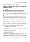
Figure 1.1 SHRP Regions ........................................
6
Figure 2.1 SHRP-LTPP Profilometer Field Activity Report--SPS ...............
33
Figure 3.1 Dipstick Measurements ..................................
42
Figure I. 1 The Analysis Parameters .................................
66
Figure 1.2 The Profile in a Graphical Format for a GPS Site ..................
69
Figure I. 3 The Profile in a Graphical Format for a WIM Site .................
70
Figure 1.4 The Profile in a Graphical Format for an SPS Site .................
71
Figure III. 1 The Quarter Car Vehicle Simulation Model .....................
83
Figure III.2 Demonstration Program for Computing IRI with a Microcomputer
......
Figure III. 3 PROFSCAN IRI Computation for Profilometer and Dipstick Data .......
87
88
ix
Abstract
This manual describes procedures to be followed when measuring pavement profiles for the
LTPP program using the K.J Law Profilometer, Face Technologies Dipstick, and the rod and
level. Field testing procedures, data collection procedures, calibration of equipment, record
keeping, and maintenance of equipment for each of the profiling methods are described.
Executive Summary
The Long-Term Pavement Performance (LTPP) program is a study of pavement performance
at about 1,000 in-service pavement sections. The objectives of LTPP are to:
•
evaluate existing design methods;
•
develop improved design methods and strategies for the rehabilitation of existing
pavements;
•
develop improved design equations for new and reconstructed pavements;
•
determine the effects on pavement distress and performance of loading, environment,
material properties and variability, construction quality, and maintenance levels;
•
determine the effects of specific design features on pavement performance; and
•
establish a national long-term pavement performance data base.
LTPP will collect data on in-service pavement sections for a twenty year period. The data
collected at the test sections are stored in the LTPP Information Management System data
base. This data will be used develop improved pavement design procedures that will enable
highway engineers to tailor designs and maintenance to specific conditions.
The annual collection of longitudinal profile data of each test section is a major task of
LTPP. The left and right wheel path profile data for five repeat runs on a test section are
stored in the data base. In addition, the International Roughness Index (IRI), Mays Index,
Root Mean Square Vertical Acceleration (RMSVA) and slope variance, which are computed
from the profile data, are stored in the data base.
This manual describes procedures to be followed when measuring pavement profiles for
LTPP using the K.J. Law Profilometer, Face Technologies Dipstick and the rod and level.
Field testing procedures, data collection procedures, calibration of equipment, record keeping
and maintenance of equipment for each of the profiling methods is described. The primary
device used to obtain pavement profile measurements for LTPP is K.J. Law Profilometer.
However, when a Profilometer is not available the Dipstick is used to collect profile data. A
rod and level can also be used to measure pavement profiles if a Profilometer or a Dipstick
is not available.
1. Introduction
1.1
Overview of SHRP and the LTPP Program
The Strategic Highway Research Program's (SHRP) Long Term Pavement Performance
Program (LTPP) is study of pavement performance in different climates and soil conditions
at about one thousand in-service pavement sections in all fifty states of the United States and
in participating provinces in Canada.
For purposes of pavement data collection and coordination, the U.S. and participating
Canadian provinces have been subdivided into four regions, each served by a Regional
Coordination Office Contractor (RCOC). The regional boundaries defining the jurisdiction of
each RCOC are shown in Figure 1.1.
1.2
Significance
of Pavement
Profile
Measurements
The longitudinal profile along the wheel paths in a pavement can be used to evaluate the
roughness of the pavement by computing a roughness index such as the International
Roughness Index (IRI). The change in the longitudinal pavement profile over time, which is
directly related to the change in roughness with time, is an important indicator of pavement
performance. Hence, one aspect of the LTPP program is to collect pavement profile data of
in-place pavement sections for use in improving the prediction of pavement performance.
1.3
Profile Data Collection
The primary device used to obtain pavement profile measurements for the SHRP-LTPP
program is the Model 690DNC Inertial Profilometer manufactured by K.J. Law Engineers,
Inc. Each RCOC operates one Profilometer to collect data within its region. The operation
and maintenance of the Profilometer and the storage of the collected data are the
responsibility of each RCOC.
However, when a Profilometer is not available, SHRP has elected to use the Dipstick, which
is a hand-held digital profiler manufactured by Face Technologies to collect profile data. The
Dipstick is also used to obtain transverse profile data in some circumstances. Each RCOC
contractor maintains a Dipstick for profile data collection for these circumstances.
A rod and level can also be used to measure pavement profiles if a Profilometer or a
Dipstick is not available, or where other special circumstance or requirements rule out the
Dipstick or the Profilometer.
5
0
........
<.
•
........
O"
"
iiii!iiiii
.Z ........
W
6
1.4
Overview
of the Manual
This manual describes procedures to be followed when measuring pavement profiles using
the K.J. Law model 690DNC Inertial Profilometer, the Face Technologies Dipstick and the
rod and level. The manual covers the following:
1.
2.
3.
4.
5.
Field Testing
Data Collection
Calibration of Equipment
Equipment Maintenance
Record Keeping
This document addresses those aspects of profile measurements that are relatively unique to
the LTPP research. Other references should be consulted for general information.
7
2. Profile Measurements Using the K.J. Law Profilometer
2.1
Introduction
The K.J. Law Model 690DNC Inertial Profilometer measures the longitudinal road profile in
the two wheel paths. The system for measuring the road surface profile consists of an
optical displacement measuring system and a precision accelerometer for each wheel path.
The optical system measures the distance between the vehicle body and the pavement
surface, while the accelerometer measures the motion of the vehicle body. Signals from the
non-contact sensors of the optical system and the accelerometers are fed into a computer
which computes the profile of the pavement. The profile data is recorded on the hard disk of
the computer for further processing. The computer terminal shows the profile of the
pavement as it is measured.
The device is equipped with a photocell capable of detecting identifying marks on the
pavement surface, such as reflective tape or a white painted line. This feature is used to
initiate profile data collection. A digital distance encoder attached to the front wheel of the
vehicle accurately measures the travelled distance. A generator is provided in the vehicle to
supply power to the computer and other electronic equipment. The Profilometer vehicle is
equipped with both heater and air-conditioning units to provide a uniform temperature for the
electronic equipment carded in the vehicle. The Profilometer vehicle can measure road
profiles at speeds ranging from 10 to 55 mph (16 to 88 kmph). For the SHRP-LTPP studies,
the test speed will normally be 50 mph (80 kmph).
Three of the four Profilometer vehicles used to collect prof'tle data for the SHRP-LTPP
program are identical. They were purchased by SHRP and then sent to the regional
contractors. The vehicle used for these Profilometers is a motor home and the distance
between the non-contact sensors for these units is 66 in. (167 cm). The fourth Profilometer
vehicle, which belongs to the FHWA, has been loaned to SHRP. This unit is in a van. The
distance between sensors on this vehicle is 54 in. (137 era).
Detailed outlines of the operating procedures, calibration, and maintenance requirements of
the different components of the Profilometer vehicle can be found in the manuals listed in the
References.
2.2
2. 2.1
Operational
Guidelines
SHRP Procedures
Maintenance of Records: The operator is responsible for preparing and forwarding the
forms and records as described in Section 2.6, which relate to testing and maintenance of the
Profilometer to the RCOC.
Accidents: Insurance coverage for the operator, driver, and the vehicle is maintained by the
RCOC. The operator will inform the RCOC as soon as possible after an accident. Details
9
of the accident should be reported later in writing to the RCOC to assist in any insurance
claim procedure which might be affected.
2.2. 2 General
Operations
The following guidelines related to the general operation of the Profilometer device shall be
followed.
2.2.2.1
Temperature
Range
The interior vehicle environment is critical to the operation of the on-board computer. Fixed
head disks operate with very close mechanical system tolerances and may be damaged if
subjected to large temperature variations or extremes. The computer system should only be
operated in a temperature range of 59 to 90°F (15 to 40°C). Further, the maximum rate of
change of temperature should not exceed 20°F/hour (11°C/hour). The vehicle is equipped
with a propane furnace and an air conditioner to maintain the temperatures within the
required range. If the computer is not being operated, the storage temperature can range
from -40 to 151°F (-40 to 660C).
During periods of testing in hot weather, it is suggested that the roof vent or side window in
the work area be left ajar and the fan operating when the Profilometer is retired at the end of
the workday. If the air temperature will drop below 60°F (16°C), the propane heater should
be turned on and set to 60°F (160C).
2.2.2.2
Disk Drives
Saving fries to the hard disk or floppy disks, or loading flies from the hard disk or floppy
disks, should not be done when the vehicle is in motion as this can destroy data files. The
computer's virtual memory should be used to record all data while the vehicle is in motion.
2.2.2.3
Power Control
The power to the computer system is routed through a power controller located at the bottom
of the computer enclosure. When the controller is in the remote mode, no power will be
supplied to the rest of the equipment unless the computer is turned on. If the controller is
placed in the local mode, then individual components may be turned on and off.
2.2.2.4
External
Power Source
Power should be turned off to all instruments, computer, and the generator before connecting
to an external power source. The external electrical power cord can be connected to a
standard 30 amp outlet, or (with an adapter) to a standard 15 amp outlet. The power
requirements are 115 volts AC at 10 amperes, or 230 volts AC at 5 amperes.
When an
external power source is used, a relay will automatically switch from the generator to the
external power source. When operating on external power with the sensor lamps turned on,
10
the battery charger should be activated to keep the 12 volt batteries charged.
2. 2.3
2.2.3.1
Field Operations
Operating
Speed
A constant vehicle speed of 50 mph (80 kmph) should be maintained during a profile
measurement run. If the maximum constant speed attainable is less than this due to speed
limits, traffic congestion, or safety constraints, then a lower speed as close as possible to 50
mph (80 kmph) should be selected. If the site is relatively fiat, cruise control should be used
to maintain a uniform speed. It is important during a profile run to avoid changes in speed
which may jerk the vehicle or cause it to pitch. Change in throttle pressure or use of brakes
to correct vehicle speed should be applied slowly and smoothly.
2.2.3.2
Event Initiation
During profile data collection, the data collection program uses "event marks" to initiate data
acquisition. The event marks are generated by either a photocell event detector or by the
operator event pendant.
The photocell event detector uses the white paint stripe on the pavement prior to the test
section to initiate data acquisition. Depending on the reflectivity of the paint mark on the
pavement, the detection threshold control located on the front of the console may require
some adjustment for the photocell to trigger properly. If the pavement surface is bright, the
threshold should be lowered. If the pavement is dark the threshold should be increased.
Several passes over the section may be required to determine the proper threshold setting. In
instances where the existing paint mark on the pavement does not trigger the photocell even
with threshold adjustments, reflective pavement marking tape may be placed at the beginning
of the section.
If the threshold for the photocell has to be set near zero to enable the photocell to trigger, it
could indicate a clouded lens in the photocell. This occurs when the brass inside the
photocell corrodes and fogs the lens. The photocell has to be returned to K.J. Law for
cleaning.
Sometimes, the photocell event detector may not trigger on pavements with a light-colored
surface. If this condition occurs, the operator event pendant should be used instead of the
photocell to initiate data collection. This method requires the operator to judge the starting
point for data acquisition. A reference point near the starting point on the side of the
pavement (e.g., a road sign or a tree) should be used for consistency. Several practice runs
may be needed for data acquisition by this method.
11
2.2.3.3
Recording
Profile Data
The virtual memory on the DEC computer will be used as the recording medium during a
profile run. After the run is completed, the driver should pull over and come to a complete
stop at a safe location so the data can be transferred to the hard disk prior to another profile
run. On sections where the turnaround distance is relatively short, the operator could
complete all runs before saving the data to the hard disk. All data should be transferred to
the hard disk and backed up on a floppy disk before the crew leave the test section.
2.2.3.4
Inclement
Weather
and Other Interferences
In some instances inclement weather (rain, snow, lightning, and heavy cross winds) may
interfere with the acquisition of acceptable data. In general, profile measurements should not
be conducted on wet pavements, particularly when free-standing water is present. In some
cases, it may be possible to perform measurements on a damp pavement with no visible
accumulation of surface water. In these circumstances, run-to-run variations and potential
data "spikes" should be closely watched. A spike threshold value is used to identify spikes.
When two consecutive elevations have a difference in excess of this value and the next
elevation is such that the middle point becomes either a maximum or a minimum of the three
points, a spike is present. The Profscan program (1) uses a spike threshold value of 0.1 in.
(0.25 cm). Spikes can be due to field-related anomalies (e.g., potholes, transverse cracks,
bumps) or due to - saturation, electronic failures or interferences.
Changing reflectivity on drying pavements due to the differences in brightness of the
pavement (light and dark areas) will often provide results inconsistent with data collected on
uniform colored (dry) pavements. This could be due to varying accuracy of the light sensing
unit due to the rapid changes in reflectivity or to the dark spots resulting from marginal lost
lock situations. In such situations, profile measurements should not be performed until the
pavement is dry.
In some instances, electromagnetic radiation from radar or radio transmitters will interfere
with operations and data recording. If this occurs, the operator should attempt to contact the
source to learn if a time will be available when the source is turned off. If such a time is not
available, it may be necessary to schedule a Dipstick survey of the test section.
2.2.4 Number of Runs
This section describes the procedures to be followed to obtain an acceptable set of profile
data.
2.2.4.1 IRI from DEC
The DEC computer in the Profilometer vehicle records the profile data and computes the IRI
of the test section. The IRI of the left wheel path and the right wheel path, as well as a
both-wheel path IRI, which is the average of the left and right wheel path IRI are computed.
12
During each run, the DEC terminal displays the profile of the left and the fight wheel paths.
Immediately after the run is completed, the terminal displays the computed IRis and a hard
copy of the profile with the IRI values is printed. Before saving the profile data, the operator
should enter any comments regarding the completed run that may affect the measured data.
These include: failure to maintain correct wheel path; whether saturation light or lost lock
light was on; passing trucks; high winds; and rapid acceleration or deceleration.
The degree of run-to-run variability in IRI within a section under normal operating conditions
will usually depend on the roughness of the pavement. On new asphalt concrete overlays or
new concrete pavements, variation of IRI between runs will be very small. However, rough
pavements may cause more variability in IRI between runs. If during testing the operator
notes very high run-to-run variations of IRI between runs, testing should cease and the cause
of variation should be identified. If the variation is due to equipment problems (e.g., worn
shroud cover), the problem should be corrected. If the variations are due to causes beyond
the operator's control, such as radar interferences or low sun angle, the operator should
decide how to proceed with testing. For example, if the sun is low, the operator could wait
until conditions improve and perform testing or leave the test location and test' itat a later
time.
Once the operator is confident that a minimum of five error-free runs have been completed,
the acceptability of the prof'de runs has to be evaluated using the Profscan program (1).
2.2.4.2
IRI from Profscan
The acceptability of the runs performed by the Profilometer vehicle is evaluated using the
Profscan program. The user manual for Profscan is included in Appendix I. Profsean runs on
an IBM compatible computer and cannot be run on the DEC machine. The profile data
recorded in the DEC is converted to a form that can be read by an IBM compatible machine
using the Kermit program. The Kermit program can be called from the Main Menu (see
Section 2.3.4).
The Profsean program should be set to the following parameter settings:
Spike Threshold Value: 0.10 in
Summary Interval: 100 ft
Seed (36 ft into run): 'Y'
% Tolerance on Mean: 1.0
% Tolerance of Standard Deviation: 2.0
The Profscan program uses the profile data to compute IRI for the left and fight wheel paths,
as well as a both-wheel path IRI which is the average of the left and fight wheel path IRis.
The Profscan program also generates a report of spikes present in the pavement profile.
There is a small difference between the IRi computed from the program in the DEC
computer and Profscan due to a differences in data initialization in the computer programs.
13
A minimumof five profile runs should be used with Profscan. If more than five runs are
available at a site the user has the option of selecting five runs to be analyzed by Profscan.
The prof'fle runs at a site are accepted by the Profscan if the average IRI of the two wheel
paths satisfy the following criteria.
1.
The IRI of three runs are within 1% of the mean IRI of the selected runs.
2.
The standard deviation of IRI of the selected runs are within 2% of the mean
IRI.
If the IRI from the profile runs meet the Profscan criteria and the operator finds no other
indication of errors or invalid data, no further testing is needed at that site.
2.2.4.3
Non-Acceptance
of Runs by Profscan
If the runs do not meet the Profscan criteria, the operator should perform the following two
steps to identify if the variability is the result of equipment/operator errors or pavement
related.
1.
Review the end-of-run comments of the runs as well as the following factors to
determine if any of these factors could have affected the data collected during
the profile runs. The factors to be considered are: whether saturation light or
lost lock light was on, low sun angle, worn shroud cover, passing trucks, high
winds, rapid acceleration or deceleration of vehicle.
2.
Review the spike report generated by Profscan to determine if the spikes are
the result of field-related anomalies (e.g., potholes, transverse cracks, bumps)
or due to saturation, electronic failures or interferences. This can be analyzed
by reviewing the Profscan reports and seeing if the spikes occur at the same
location in all runs.
If the variability between runs or the spikes are believed to be operator or equipment error,
identify and eliminate, correct, or avoid (as in the case of non-ideal lighting conditions) the
cause of the anomalies and make additional runs until a minimum of five runs free of
equipment or operator errors are obtained. Where anomalies in the data are believed to be
due to pavement features, rather than errors, a total of nine runs should be obtained at that
section. If the data from the last four runs are consistent with those for the first five (in
terms of variability and the presence of pavement-related anomalies), no further runs are
required. If the data from the last four runs differ from those for the first five runs, the
operator should reevaluate the cause of the variability or apparent spike condition, and make
additional runs until five error-free runs have been obtained. Once testing is completed, the
Profscan program should be used to evaluate the data.
14
2.2.5
Labelling
Disks
Disk labeling standards are important so that all personnel will be able to understand where
the data originated based on the disk label. Labels will be created using the following format
for GPS sections:
1.
Line 1: "/D# xxxxxx" where xxaxxx is the SHRP section number.
2.
Line 2: "Volume x ofy'" where x is the number of the current disk in the set
and _ is the total number of disks in the set.
3.
Line 3: "Copy # x" where x is the number, usually 1 to 3.
4.
Line 4: "Profilometer SNxxx" where xxx is the serial number of the
Profilometer vehicle.
5.
Line 5: "MM/DD/Y'P' where MM/DD/YY is the month, date and year that the
testing was performed.
Example:
GPS Section
ID# 263456, 264567, 265678
Volume 1 of 1
Copy 1 of 3
Profilometer SN 007
Date 08/28/91
The above label tells that the data was collected from GPS sections 263456, 264567 and
265678 on August 28, 1991.
2.3 Field Testing
2.3.1 General Background
Collection of profile data is the primary responsibility of the Profilometer operator. The
procedures to be followed each day prior to and during data collection with respect to daily
checks of vehicle and equipment, start-up procedures, setting up the software for data
collection and using the software for field data collection are described in the following
sections.
The following sections will describe the procedures to be followed when testing General
Pavement Studies (GPS) sections. Some of the procedures to be followed for testing Specific
Pavement Studies (SPS) sections are different than the procedures for GPS sections. Section
2.7 of this/nanual outlines the procedures for SPS sections which differ from the procedures
for GPS sections.
15
2.3. 2 Daily Checks on Vehicle and Equipment
The operator should use Daily Check List form given in Appendix V to check the vehicle
and the generator at the start of the day. It is important to maintain the equipment at a proper
operational temperature as noted in section 2.2.2.1. If the weather is very damp, the heater
should be turned on to remove moisture from inside the unit. The sensor and receiver glass
may require cleaning more than once during the day.
2.3.3
Starting
the Generator
The following procedure should be used for starting the generator.
16
1.
Before starting the generator, ensure that all external power sources are
disconnected and that all instruments and the computer are turned off.
2.
Depress the Start/Stop rocker switch to start the generator. Release the switch
when the engine starts. If the generator does not start in a few seconds, wait
ten seconds and try again. If further difficulty is encountered, consult the
operator's manual for the generator.
3.
Once the generator is operating, wait for a few minutes to allow the generator
to come up to speed and to stabilize. If the temperature is cool and damp, or
cold, turn the air intake to winter conditions. If the idle is rough, adjust the
fuel-to-air mixture (adjustment on float bowl) to obtain the ideal setting. If the
generator still runs roughly, the operator may have to clean the carburetor of
the generator. Consult the operator's manual for the generator for details. If
the generator still runs roughly, it may need to be serviced.
4.
Any equipment which uses power supplied by the generator should not be
turned on until the generator has stabilized. A clicking sound indicates that the
generator has stabilized and that it is safe to turn on the various equipment
powered by the generator. If the voltage on the auxiliary battery has dropped
below 12 volts, turn on the charger for the auxiliary battery. The battery
charger is mainly used to keep batteries charged when the unit is plugged to an
external power source or to provide additional charge to increase the intensity
of sensor lights when testing pavements with dark surfaces. NOTE: Do not
turn on auxiliary battery charger if the vehicle has a solenoid that ties the
vehicle's main and auxiliary batteries and charges them at the same time.
5.
Warm up the system prior to performing calibration checks or performing
tests. This may be as little as 15 minutes in the summer or as much as 30
minutes in the winter.
2.3.4
Setting Up the Software
Ensure that the ambient temperature and rate of change of temperature within the vehicle is
within the system operating range (see Section 2.2.2.1). Proceed in the following order:
1.
Place the system disk in the upper drive (DU1) of the DEC computer. Make
sure that the write-protect notch is on the left side.
2.
Turn on the computer or press the nRestart" button if power is already on.
The system will access the disk and load the operating system into memory.
Verify that the run light is on and the DC OK light is illuminated.
3.
If the monitor does not respond, then:
a.
Depress the "Restarff button on the DEC PDP 11/83 front panel.
b.
Depress and hold [Ctrl] and then press C. Do this twice.
e.
Within one minute the terminal should respond with:
Message 04 Entering Dialog Mode
Commands are Help, Boot, List, Setup, Map and Test
Type a command then press the IRETURN1 key.
d.
Type "BOOT DUI" and press the [Return] key. The upper drive
indicator should light, indicating that the disk is being accessed.
e.
If the start up message does not appear within one minute, boot the
system with the backup system disk.
f.
If the system still does not respond, or the "Halt" indicator light comes
on, the DEC computer needs servicing. This should be performed by
an authorized DEC service center.
Once the software has been loaded, remove the system disk from the drive. The monitor will
display the M_n Menu:
A
B
C
D
E
F
G
I
FORMAT AND INITIALIZE (calls the format - initialize menu)
RUN BACKUP (calls the file backup menu)
RUN CALIBRATE (runs the calibrate program)
LIST DIRECTORIES (calls the directory menu)
TIME DATE (permits changing time and/or the date)
RUN REPLAY (runs the profile replay utility)
HEADER MENU (lists, deletes and copies header flies)
TRANSFER FILES TO IBM (calls the KERMIT routine to transfer files to a format
that can be read by a IBM- compatible computer)
17
P
H
X
RUN PROFILE (runs the profile program)
PRINT HELP FILE (prints the HELP file)
Exit
All commands are executed by typing the appropriate letter from the menu and then pressing
the [Return] key. If the operator makes a mistake, the typed character can be deleted with
the [Backspace] key.
2.3.5
Calibration Checks
The following calibration checks should be performed before profile measurements are taken.
1.
2.
2.3.5.1
Displacement Sensor Check
Bounce Test
Displacement Sensor Check
The displacement sensor check is a test of the non-contact displacement sensors to determine
if they are within tolerance. Distances from the vehicle body are measured during this test,
so extreme care must be taken to ensure that the vehicle is absolutely still during this check.
If any movement occurs during this check, for example due to wind, it may be necessary to
move the vehicle to an enclosed building, or park it on the side of a building protected from
the wind. The displacement sensor check should be repeated separately for left and right
sensors. To initiate the displacement sensor check, select "C", Run Calibrate, from the Main
Menu (see Section 2.3.4). Then the following menu will be displayed.
K
D
A
L
R
B
S
G
X
W
X
Enter Scale Factor Via Keyboard
Record all Scale Factors on Disk
Accelerometer Calibration
Left Displacement Sensor Calibration
Right Displacement Sensor Calibration
Display Profile for Bounce Test
Display Left and Right Displacement Sensors
Display Accelerometer Outputs
Display Rate Gyro Output
Wheel Encoder Calibration
Exit Program
The following steps are to be followed during the displacement sensor check.
18
1.
Enter "R" and [Return] to start the non-contact sensor calibration for the right
sensor ("L" for the left sensor).
2.
A prompt to insert the calibration plate under the light source and to level it is
then displayed. Place the calibration plate below the light source. Level the
plate by adjusting the three leveling screws until the bubble on the plate is
centered. If the plate cannot be leveled because of rough pavement grade,
move the vehicle to a more level and smooth surface.
3.
After the plate is levelled, enter "Y" and [Return], which signals the
computer to take 200 readings and compute a mean for the lower level.
4.
The computer program will then prompt for the insertion of the 1.0 in. (2.5
cm) block. Carefully place the block on the plate, under the light source.
Enter "Y" and [Return]. The program will then take 200 readings and
compute a mean for the upper level. Then, the difference between the means
of the lower and upper levels will be computed. If this difference is within +/0.01 in. (+/-0.25 mm) the sensor has passed the calibration check.
5.
If the differences is more than +/-0.01 in. (+/-0.25 mm) a message that the
calibration value is out of tolerance is displayed.
6.
Enter "N" to the question if a new calibration factor is to be computed and
repeat the calibration procedure until the difference of readings is within
tolerance (repeat calibration procedure a maximum of 3 to 4 times to achieve
this condition).
7.
If a difference of readings within tolerance cannot be achieved (after repeating
the calibration procedure 3 to 4 times), answer "Y" to the prompt if a new
calibration factor is to be computed.
8.
Save this computed calibration factor in the virtual memory. Also complete the
form Prof'dometer Calibration Log (see Appendix V) and note that it is a field
calibration. This calibration factor is used for tests that are performed.
However, this factor will be lost when the power to the computer is turned
off. NOTE: The calibration factor computed during the field displacement
sensor check should not be saved on the system diskette.
If difficulty is encountered with calibration or checking of the non-contact sensors, it may be
beneficial to check the light output with the oscilloscope for proper signal magnitude and
alignment.
2.3.5.2
Bounce Test
The bounce test is used to check the accelerometers which senses the movement of the
vehicle body. The following procedure is used to conduct this test.
1.
Park the vehicle.
2.
From the Main Menu (see Section 2.3.4) select "P" (run profile).
3.
Answer "Y" to the question "Do you want to record profile".
19
4.
Answer "N" to the question "Do you want to use an existing header file".
5.
Then the Surface Profile Setup Menu (see Section 2.3.6.1) will be displayed.
In this menu select "T" and enable the Test Mode Oscillator.
6.
Proceed to the Run Identification Menu (see Section 2.3.6.2) and input any
arbitrary six characters to the section number.
7.
Proceed to the Run Control Method Menu (see Section 2.3.6.5)
Start Method Pendant and Stop Method Pendant.
8.
Proceed to Options Setup Menu (see Section 2.3.6.6) and change the wheel
path as both and the averaging interval to 100.
9.
Proceed to the System Change Setup Menu (see Section 2.3.7) and press
[Return] to enter the run mode.
10.
Depress the start pendant, then exit the vehicle. Stand on the rear bumper of
the vehicle and rock the vehicle back and forth, and side to side by shifting
your weight from foot to foot.
11.
During this "bouncing" of the vehicle, the output displayed in the monitor
should remain static and show no or very little variation. The stop pendant
should then be depressed after 15-30 seconds.
12.
The computed
usually this is
surface. If the
the procedure
2. 3. 6 Entering
Header
and select:
IRI should normally be less than 5. If the IRI exceeds 10,
the result of lost lock. Perform the test again, but on a different
IRI is still high, the accelerometers should be calibrated using
outlined in Section 2.4.3.
Information
Before testing a section, the operator has to go through a series of header menus in the
software and input data relevant to that section as well as change several default settings in
these menus.
Before beginning this process the operator should complete the following:
20
1.
Make sure that the computer shows the current date and time.
2.
Check that the power is supplied to the sensors and sensor lamps. The lost
lock lights should be lit if power is not supplied. After supplying power it may
take a few moments before the lost lock lights go out. If the lost lock light is
on continuously the bulb may be burnt.
3.
The shrouds must be lowered to approximately 1 in. (2.54 cm) from the
pavement to keep the sun from washing out the signal to the displacement
receivers.
To begin the process of entering header information select up. and [Return] if in the Main
Menu (see section 2.3.4) or type "Run Profile" and [Return] from the monitor. The program
will first load the system calibration factors from the disk. If the file containing the
calibration factors (SCALE.CAL) is not found or if there is an error in reading the data, an
error message will be displayed. If this occurs, the operator should re-boot the computer,
making sure that the vehicle is stationary during the booting period. Frequently the error
message occurs because the file SCALE.CAL is not copied to the memory and all that is
needed is for the operator to copy SCALE.CAL to the virtual memory.
Once the scale factors are read, the program will prompt the operator with the following
questions:
1.
"Do you want to record profile." The operator should respond with a ,yu and
[Return].
2.
"Do you want to use an existing header file." The operator can respond with
a "Y" or "N". If the operator types "Y", the program will generate a request
for a header file name. Once the operator enters a file name, the parameters
stored in the file will be read and the program will advance to the main menu
where it is possible to go dlrecfly to profile computing mode or to modify the
parameters read from the file. When using an existing header, the section
number under the Run Identification Menu (see Section 2.3.6.2) must be
reentered to update the DEC automatic file date sequence because the Profscan
program uses the date to match files with headers. If this is not done an error
message will appear when using Profscan. However, usually the operator will
answer "N".
If the operator responds with "N", this answer will take the operator through the following
header generation menus.
1.
2.
3.
4.
5.
6.
Surface Profile System Setup
Run Identification
Run Location
Run Conditions
Run Control Method
Options Setup
The first menu to be displayed when the operator answers "N" to the question "Do you want
to use a existing header ?_ is the Surface Prof'tie System Setup.
21
2.3.6.1
Surface
Profile
System
Setup
The structure of this menu is shown below.
DATE DD - MM - YY
A
B
C
D
E
H
P
T
TIME HH:MM:SS
DRIVER DISPLAY UNIT MILES
FILTER WAVELENGTH 300, (fee0
GRAPHIC SCALE 1.00 (inches)
GRAPH LENGTH 800 (feet)
PRINT LAST SCREEN ON EXIT ENABLED
HELP
FORM FEED
TEST MODE OSCILLATOR DISABLED
enter LETrER
for option, RETURN to proceed, or X to exit
The only item that needs to be changed in this menu is the driver display unit, which must
be changed to feet. To make this change select "A" and [Return] to toggle the display units
to feet. Thereafter, press [Return] to proceed to the next menu.
2.3.6.2
Run Identification
A
B
D
C
G
H
E
SECTION NUMBER 263456
RUN NUMBER 1
SHRP FILE NAME 26345691.031
DEC FILE NAME B63456.D91
AUTOMATIC DEC FILE NAME GENERATION ENABLED
AUTOMATIC DEC FILE NAME INCREMENTS ENABLED
OPERATOR/DRIVER
xxxxxxxxxxxxxxxx (16 MAX)
enter LETrER for option, RETURN to proceed, or X to exit
In this menu the section number and the operat0r/driver fields have to be completed. To
input the current test section number, the operator should press "A" and [Return]. The
program will then accept the entry of the six-digit test section number for the GPS section
(e.g., 263456). The SHRP file name and DEC file name will be automatically generated
(SHRP f'de name 26345691.031, DEC file name - B63456.D91). The DEC computer
filename will be the same as the SHRP six-digit section number for GPS test section. The
operator will then select the letter "E" and [Return] to enter the operator/driver names. Upon
completion of this menu press [Return] to proceed to the next menu.
2.3.6.3
Run Location
A
B
22
ROAD DESCRIPTION xxxxxxxxxxxxxxxxxxxxxxxxxxxxxx
LANE MEASURED xxxxxxxxxxxxxxxx (16 MAX)
(32 MAX)
C
D
E
F
DIRECTION xxxxxxxx (8 MAX)
HORIZONTAL OFFSET xxxxxxxxxxxx (12 MAX)
BEGINNING DESCRIPTION xxxxxxxxxxxxxxxxxxxxxxxx (24 MAX)
ENDING DESCRIPTION xxxxxxxxxxxxxxxxxxxxxxxx (24 MAX)
enter LETTER for option, RETURN to proceed, or X to exit
All items in this menu must be completed. Entering the appropriate letter and pressing
[Return] allows the insertion of the required entry. Each entry is terminated by the [Return]
key. For road description enter the route number. After filling in the appropriate data press
[Return]to access the next screen.
2.3.6.4
Run Conditions
A
B
ROAD SURFACE MATERIAL xxxxxxxx (8 MAX)
ROAD CONDITION xxxxxxxx (8 MAX)
WEATHER
C
D
E
TEMPERATURE
xxxxxxxx (8 MAX)
CLOUD CONDITION xxxxxxxx (8 MAX)
OTHER xxxxxxxxxxxxxxxxxxxxxxxx (24 MAX)
enter LETTER for option, RETURN to proceed, or X to exit
Enteringthe appropriateletter and pressing [Return]allowsthe insertionof the required
entry. Each entry is terminatedby the [Return]key. The road surface material should be
entered as A-CC if the surface material is asphalt, or as P-CC if the surface material is
concrete. The road condition should describe the surface condition of the pavement. The
surface condition can be described as v. good (very good), good, fair or poor depending on
the observed surface defects. The temperature should be the air temperature at the time of
test. The cloud condition can be described either as clear, p. cloudy (partly cloudy) or
cloudy. The Other field is used to indicate conditions that interfere with the data collection
process such as high traffic volumes, wind conditions and high intensity of the sun. Upon
completion of this menu, press [Return] to proceed to the next menu.
2.3.6.5
Run Control Method
A
B
START METHOD PENDANT
STOP METHOD PENDANT
enter LETTER for option, RETURN to proceed, or X to exit
This menu is used to select the start and end methods for the profile run. Select the start and
stop method using the following steps.
1.
"A" toggles between pendant and photocell.
23
2.
nB" toggles between pendant, photocell, and distance. When distance is
selected as the ending method, the operator is prompted to enter the length of
the run.
The photocell event detector should be used as the start method where possible. If the
photocell event detector cannot be used (e.g., light colored pavement surface), the operator
event pendant should be selected. The stop method to be used is "distance" irrespective of
the start method. For GPS sections a distance of 500 feet should be used for the length of
the run. Upon completion of this menu press [Return] to proceed to the next menu.
2.3.6.6
Options
I
R
W
A
B
E
S
Setup
INDEX ENABLED
RIDE QUALITY INDEX IRI
WHEEL PATH RIGHT
AVERAGING INTERVAL 500 (feet)
INDEX CALCULATION SPEED 50.0 (mph)
FILTER REINITIALIZATION DISABLED
STORE HEADER OPTIONS
enter LETTER for option, RETURN to proceed, or X to exit
The fields wheel path and averaging interval need to be changed in this menu. Wheel path
should be set to "BOTH" to cause the computed ride quality index to be displayed as the
average across both wheel paths. This is done by pressing "W" and [Return] twice. The
averaging interval should be changed by pressing nan and then entering 100. When the Index
Option switch is set to "ENABLED" the DEC computes the specified ride quality index.
When the Ride Quality Index is set to IRI, the International Roughness Index (IRI) is
computed for each run. The Index Calculation Speed, which is used to compute the ride
quality index, should always be set to 50 mph regardless of the measurement speed of the
Profdometer.
2.3.7
Data
Collection
Once all the header menus are completed, the System Change Setup Menu will be displayed.
SYSTEM CHANGE SETUP MENU
A
B
C
D
E
F
H
S
24
SYSTEM SETUP
RUN IDENTIFICATION
RUN LOCATION
RUN CONDITIONS
RUN CONTROL
OPTIONS SETUP
RECALL EXISTING HEADER
STORE HEADER SETUPS
enter LETI'ER for option, RETURN to RUN, or X to exit
Choices "A" through "F" sends the operator to the menus previously discussed. After all of
the header file information has been entered, the header file should be saved to the virtual
memory and the hard disk (DU3). This is done repetitively by selecting "S" from the menu
and then selecting the appropriate drive and entering the six digit test section number at the
prompt.
The profile data collection program has to be started to begin data collection. Make sure that
a SHRP-LTPP Profilometer Field Activity Report form (see Appendix V) is ready to record
the DEC IRis. To start the profile data collection program, press [Return] from the System
Change Setup Menu.
Once these steps are completed, the Profilometer device is ready to take measurements.
following steps should be followed during profile measurements.
The
1.
About 2,000 ft. (610 m) before the test sectionstart the profile data
collection program. A graphical display is then generated with the message
"Not Recording".
2.
The guidelines given in Section 2.2.3.1 regarding the operating speed should
be followed. The driver should attain the constant test speed at least 300 feet
(91.5 m) before data collection begins.
3.
Press the start pendant to arm the photocell after passing the lead in stripe
located before the test section. The message Nphotocell alert" is displayed on
the monitor.
4.
Once
starts
lights
mark
5.
After the test section has been traversed and the computer has computed the
DEC IRI, write the value on the SHRP-LTPP Profilometer Field Activity
Report Form (see Appendix V). Note any factors that could have affected the
computed IRI in the Profilometer Field Activity Report Form.
6.
After the computer gets out of the profile display mode, type any comments
pertaining to the run (e.g., lost lock or saturation lights come on during the
run, any other factors that could affect the measured profile) and then press
[Return].
7.
Thereafter, the driver should stop the vehicle at a suitable location so the data
can be saved on the hard disk. This should be done immediately after each run
since the profile data stored in the virtual memory can be lost if the power to
the computer fails. Where turn around distances are relatively short, the
the event
from the
come on
is passed,
mark is detected, the
beginning of the grid.
during the run. If the
follow the procedure
display is erased and the recorded profile
Observe if the lost lock or saturation
photocell does not trigger when the event
outlined in Section 2.2.3.2.
25
operator may wait to transfer the data to the hard disk until all runs have been
completed.
2.3.8
8.
Follow the procedures outlined in Section 2.2.4 to obtain a set of acceptable
runs at a site.
9.
Once testing at a site is completed make backup copies as outlined in Section
2.3.8. The order to be followed in turning off the equipment is: (1) IBM
compatible computer (2) other devices (3) arrow board (4) sensors and (5)
DEC computer. The operator should verify that the form "Status of the
Region's Test Section" (see Appendix V) is filled before leaving the test site.
Data Backup
All prof'de data is to be backed up to a floppy disk from the DEC computer immediately
after testing is completed at a section. The operator should also create a backup copy of all
Profile test data on a IBM-compatible disk. The Profile data collection crew should not
leave a test site unless all data has been backed up. At the end of each day, an additional
two complete backup copies will be made of all Prof'dometer test data on IBM-compatible
floppy disks. These additional copies must be removed from the vehicle whenever testing is
not in progress.
The system diskette containing the Profilometer operating program and configuration files
should be removed from the vehicle when the operator is not with the equipment. New
backup copies must be made each time a change is made to the calibration factors.
2.4
Calibration
2.4.1
General Background
The non-contact sensors on each Profilometer device were initially calibrated by the
manufacturer to an accuracy of +/-0.01 in (+/-0.25 mm). The DMI (encoder) is initially
calibrated to an accuracy of 0.47%. The calibration of the non-contact sensors,
accelerometers and the distance encoder has to be done periodically to ensure that accurate
data is being collected. However, the calibration of this equipment should be done whenever
problems are suspected. The relatively stable nature of the Profilometer electronics would
indicate monthly calibrations are sufficient. Any changes in the calibration factors obtained
during calibration should be noted in the Profilometer Calibration Log (see Appendix V). All
calibrations should be performed indoors on a level surface using an external power source.
2.4. 2
Calibration
of Non-Contact
Sensors
The calibration procedure is essentially the same as that described in Section 2.3.5.1, except
for the following changes. If the difference between the two readings is within tolerance (see
step 5, Section 2.3.5.1), the calibration factor need not be changed. However, if a message
26
is displayed indicating that the difference is not within tolerance (see step 5, Section 2.3.5.1),
a new calibration factor should be obtained. Answer "Y" to step 6 in Section 2.3.5.1 to
obtain the new calibration factor. This new calibration factor should be saved on the system
disk and the backup system disk. If the factor is not saved, it will be lost when the
calibration program is exited. This factor should also be noted on the Profilometer
Calibration Log (see Appendix V).
2.4.3
Calibration of Accelerometers
The accelerometer has a special calibration coil wound on the sensing mass of the transducer.
A current through this calibration coil exerts a force on the sensing mass which is interpreted
by the accelerometer as an acceleration. The analog accelerometer electronics are designed
so that the computer can switch a precise current through the calibration coil to represent
exactly lg (32.172 ft/sec 2 or 9.81 m/see2). The calibration coil is aligned with the sensing
axis of the accelerometer so that accurate calibration can be performed even if the vehicle is
not level. An accelerometer "scale factor" is computed so that the AID converter output
change, due to the coil current representing lg excitation, when multiplied by the "scale
factor" results in exactly a lg change. During calibration the displacement of the vehicle
body is measured. Therefore, care must be taken so that the vehicle does not move during
the calibration test. The following steps should be followed to calibrate the accelerometers.
1.
From the Main Menu (Section 2.3.4) select "C" followed by Return] to enter
the calibration menu. The menu shown in Section 2.3.5.1 is displayed.
2.
Enter "A" and [Return] to start the accelerometer calibration. When this
command is entered, the program takes 200 readings of each accelerometer,
then computes and displays the mean as the zero value on the monitor.
3.
Turn on the lg test current to each accelerometer. This causes 200 more
readings to be taken on each accelerometer. The lg mean is computed and the
program takes the difference between the means for each accelerometer.
4.
If the lg values are more than 1% away from nominal values, a message that
calibration values are out of tolerance is displayed.
5.
If "Y" is the response to the prompt for new scale factors, the new scale
factors are computed and stored in memory.
6.
This scale factor should be saved on the system disk as well as on the backup
system disk. The new scale factors will be lost if the program is exited without
saving the factors.
2.4. 4 Calibration of Front Wheel Distance Encoder
Distance travelled by the vehicle as well as the vehicle velocity are measured by an encoder
mounted on the left front wheel. The encoder output is demodulated by the distance encoder
27
signal conditioning board and provides pulses to the computer for the computation of
distance. The distance encoder produces two signals in quadrature (one signal is delayed by
90 degrees) at 20 pulses per 1 ft. (0.3 m) traveled. The quadrature detector signals allows
true detection of motion in the presence of vibration in the encoder assembly.
To perform the encoder calibration, an accurately measured section 1,000 ft (305 m) to a
mile ( 1610 m) long must be utilized. When it is logistically impossible to use an existing
section (e.g., one established by a state highway agency) a new section will have to be
measured out. A tape measure should be used to measure out a 1,000 ft (305 m) section on
a reasonably level pavement with low traffic volume. In this section the start and the end
should be clearly marked. A right-angled square which is set flush with the door of the
vehicle should be used to accurately locate the starting point of the test section. Use this
same method at the end of the test section to accurately locate the end position. This
procedure will ensure that the vehicle will accurately traverse the distance set out at the site.
The following steps should be followed when performing the calibration.
1.
From the main menu (Section 2.3.4) enter "C', followed by the [Return] to
get into the calibration menu. The menu shown in Section 2.3.5.1 will now
displayed.
2.
Enter the letter "W" and [Return].
3.
The monitor will display the message:
"Driver display to be in feet or miles?"
The operator should select the feet option. The program will then display the
current distance encoder scale factor as read from the disk. The factor has
units of feet per 100 pulses (i.e., 20 pulses per foot is 5 ft per 100 pulses).
4.
The program will display the following options:
a.
b.
e.
"Drive a Measured Distance" (Type 'D')
"Simulate Distance encoder with Oscillator" (Type S)
"Exit" (Type 'E')
Select "D" and [Return] which will require the vehicle to be driven over a
measured distance.
28
5.
Start the distance measurement with the pendant and slowly traverse the
section. End the distance measurement with the pendant. The operator will
enter the length of the section in feet.
6.
The program will then compute a new scale factor. The operator will have the
option of saving this new scale factor on the system disk before exiting the
program and returning to the main program.
2.5
2.5.1
Equipment
Maintenance
and Repair
General Background
The responsibility for equipment maintenance and repair rests with each RCOC. The
decisions required for proper maintenance and repair should be based on the testing schedule
and expedited as necessary to prevent disruption of testing. Maintenance activities should be
performed prior to mobilization for testing. During a testing period there will be little time to
do more than the required daily checks prior to testing. Specific, detailed maintenance
procedure are contained in the manuals provided with each piece of equipment (see
References). The operator must become familiar with the maintenance recommendations
contained in all equipment manuals. Maintenence/repair work to be performed can be
classified as: routine maintenance, preventive maintenance and unscheduled maintenance.
2.5.2
Routine Maintenance
Routine maintenance includes work that can be easily performed with minimal disassembly of
an equipment by the operator. The Daily Check List (see Appendix V) includes a list of
maintenance activities to be performed every day. These procedures include checking the
fluid levels in the vehicle, checking the battery cable connections, checking vehicle lights,
and checking tire pressure which is required for accurate distance measurement. These items
are the most basic and easily performed maintenance measures and should always be done
prior to using the equipment every day.
2.5.3
Scheduled
Major Preventive
Maintenance
Scheduled major preventive maintenance services will include much more than the routine
checks. These service will require some disassembly of the equipment and will require
capabilities beyond the skill of the operators and RCOC staff. The SHRP Major
Maintenence/Repair Report Form (see Appendix V) will be used by the operator to report the
necessary services performed and will also serve to inform the RCOC of the condition of the
Profilometer vehicle on a regular basis.
2.5.4
Unscheduled
Maintenance
These are unscheduled repairs. These repairs must be reported on the SHRP Major
Maintenance/Repair Report form as an unscheduled maintenance activity.
2.5.5
Specific Repairs
Procedures
1. Non-Contact Sensor Lamp Replacement
1.
Turn off the power to the sensor lamps.
2.
Loosen the Allen head screws (#8) which hold the cylindrical sleeve
29
containing the 100 watt lamp.
3.
Mark the position of the adjustable block so that it will be easier to
reinstall. Loosen the two flat head screws holding the lamp and remove
the burnt out lamp.
4.
Install the new lamp, making sure not to touch it with the fingers.
5.
After tightening the lamp, install the adjustable block and make sure
that it is back in its original place.
2. Non-Contact Sensor Lamp Adjustment
2.6
Record
1.
Turn on the power.
2.
Hook the oscilloscope to the panel. Channel 1 - reference,
road.
3.
Adjust the scope to center road pulse between the two reference pulses.
Adjust light height and location to obtain maximum light intensity or
peak on the oscilloscope, using either a smooth concrete or asphalt
surface as the reference plane. The peak should be about 2/3 of that
obtained from the reference light source. Typically reference pulses
will be 12-15 volts and pavement pulses 4-6 volts. The aperture on the
camera lens can be used to adjust the light source up or down. It is
normally set one notch from fully open. The final step should be to
focus the light source for maximum intensity by using the focus
adjustment provided on the lens.
4.
Calibrate the lamp using the calibration procedure outlined in Section
2.4.2.
Channel 2 -
Keeping
There are seven reports that should be forwarded to the RCOC by the Profilometer vehicle
operator. The seven reports that are required axe as follows:
1.
2.
3.
4.
5.
6.
7.
30
Daily Check List
SHRP-LTPP Major Maintenence/Repair Activity Report
SHRP Profilometer Maintenance Data - Gasoline
Profilometer Calibration Log
SHRP/LTPP Profilometer Field Activity Report
Status of the Region's Test Sections
PROFSCAN Reports
2. 6.1
Daily Check List
In order to maintain the Profilometer device and various associated equipment in proper
operational conditions, a daily check of all items covered in the Daily Check List Form (see
Appendix V) should be performed. The operator should check off each listed item as being
within correct operational levels or conditions as stated in the operating manuals.
2. 6. 2 SHRP-LTPP
Major Maintenence/Repair
Activity Report
The vehicle and equipment operating costs are monitored with this form. All maintenance
and repairs performed on the vehicle or equipment should be reported on this form (see
AppendixV). These include scheduled maintenance as well as unscheduled maintenance.
This form should be submitted along with all receipts for maintenance activities.
2. 6. 3 SHRP Profilometer
Maintenance
Data - Gasoline
The Maintenance Data - Gasoline Form (see Appendix V) is used to monitor the gasoline
consumption. When f'tlling the form the Profilometer vehicle identification number is used as
the serial number. The RCOC for the region, names of crew members, the number of
gallons of gasoline purchased, the cost of the purchase and the odometer reading need to be
recorded in this form.
2.6. 4 Profilometer
Calibration Log
All calibrations should be recorded by the operator in the Profilometer Calibration Log (see
Appendix V). The procedures for performing these calibrations are outlined in Section 2.4.
After performing each calibration test the operator should enter the old scale factors and, if
needed, the new scale factors on this form. This form should also be filled if a new scale
factor is computed during the calibration checks performed prior to testing each day (see
Section 2.3.5.1).
2. 6.5
SHRP-LTPP
Profilometer
Field Activity Report
The Field Activity Report (see Appendix V) records all activity to and from a site, as well as
activities at the test site. Section identification information, DEC IRis as well as any factors
which might affect test data interpretation that could not be recorded in the computer are
noted in this form. The Field Activity Report should be filled out for all travel days, all
testing days, and any time operator performs maintenance on the equipment. It is important
that reports for test days be completely filled out with all section identification data so that
the report may be easily matched to the profile data. For travel only days, the section for
which the traveling is being done should be noted. This form also includes a space for the
Profilometer operator to acknowledge that the Daily Check List (see Appendix V) was
performed on the equipment and the vehicle.
31
2.6. 6 Status of the Region's
Test Sections
The Status of the Region's Test Section form, (see AppendixV) should be fdled out at every
test section. Recent maintenance or rehabilitation activities, condition of paint marks,
missing SHRP signs and delineators as well as any other comments regarding the test section
should be recorded in this form.
2.6.7
Profscan Reports
Two reports are generated for each test section by Profscan. The Summary Report contains
a statistical summary of the IRis of the different runs at a test site. The second report, the
Spike Report, contains a record of the spikes detected in the pavement profile. If no spikes
are detected at a section this report is not produced. Both these reports must be attached to
the associated Field Activity Report. The Profscan Manual (Appendix I of this book) contains
a sample Summary Report and Spike Reports.
2.7
2.7.1
Testing SPS Sections
General Background
This section describes procedures to be followed when testing SPS sites. The procedures for
testing SPS sites axe based on those used for GPS sites. This section describes the exceptions
to the GPS procedures that must be followed for the SPS sites.
A SPS site consists of a number of test sections with a transition area between the different
sections. During a Profilometer run at a SPS site, profile data are collected for the entire
site, which includes test sections as well as transition areas.
2. 7.2 Length of Test Sections
Unlike the GPS test sections which are always 500 ft (152 m), the length of SPS sites vary.
The virtual memory in the computer can only store profile data up to three miles. If an SPS
site is longer than 3 miles (4.8 km) it is necessary to test it in sections. If two files exist for
one SPS site the SHRP-LTPP Profilometer Field Report (SPS) shown in Figure 2.1 should
be filled out and attached to all generated profiles. For example, a SPS-6 site which is in
Michigan (State ID = 26), when broken into two sections, would create two fries 2606X1
and 2606X2 (see Section 2.7.6 for fde naming convention). These filenames as well as the
sub-sections contained in each file should be recorded as shown in Figure 2.1. A blank
Profilometer Field Activity Report - SPS is included in Appendix V.
32
SHRP-LTPP Prof'dometer Field Activity Report - SPS
SHRP Region:
North Central Region
State:
Michigan
SPS Section:
SPS-6
Number of Sections used in Profilometer Runs:
File Name:
2606Xl
Stations:
122+501134+001154+501177+501181
2
+50
SHRP ID:
260601
260602
260603
260604
260605
File Name:
2606X2
Stations:
291 + 00/413 + 50/424 +50/429 + 00
SHRP ID:
260606
260607
260608
260609
FileName:
Stations:
SHRP ID:
Figure 2.1. SHRP-LTPP Profilometer Field Activity Report--SPS
33
2. Z3
Operating
Speed
The guidelines described in Section 2.2.3.1 should be followed when testing SPS test
sections. When SPS sites are tested, the transition area between the sub-sections may be used
to adjust the vehicle speed to 50 mph before the next section is tested. If there is traffic in
front of the Profdometer vehicle, its speed can be initially decreased in the transition section
to increase the distance to vehicles ahead. The Prof'dometer can then be brought up to a
constant speed of 50 mph (80 kmph) before entering the next test section.
2. 7. 4 Event
Marks
Event marks are used to identify the starting point of each test section within a SPS site. The
Profscan program uses these event marks to compute the IRI of each test section.
2. Z5
Number
of Runs
Each test section within a SPS site should satisfy the Profsean criteria (see Section 2.2.4.2).
The Profscan program is capable of computing the IRI of the individual test sections within a
SPS site by identifying the test sections using the event marks. The operator should study the
IRI computed for each run to ensure that repeatable data are obtained between runs. The
procedure outlined in Section 2.2.4 for GPS sites should be followed in order to obtain an
acceptable set of runs at a SPS site.
2. Z6
Header
Generation
The procedures outlined in Section 2.3.6 for header generation for GPS test sites should be
followed for SPS test sites. However, differences exist for SPS sites in the following menus.
SurfaceProfile System Setup (see Section 2.3.6.1):
1.
The Graph Length is the length that can be seen on one screen of the monitor. The available
graph lengths are 800, 1600 and 3200 ft. Depending on the length of the SPS site select an
appropriate graph length. For long SPS sites the entire length cannot be displayed in a single
screen. For such sections, after the selected graph length is displayed, the screen is reset and
the next part of the prof'de is displayed.
Run Identification (see Section 2.3. 6. 2):
2.
The following procedure should be followed in naming the section number for SPS sections.
(a)
(b)
(c)
(d)
The
The
The
Last
III _
34
first two digits identify the state or the province.
third digit is the project code.
fourth digit is the type of SPS site.
two digits are "XX". If the SPS site is broken into two sections use "XI" and
II •
Example:
State or province : 26 (Michigan)
SPS project code : A
SPS project type : 3
Identification : 26A3XX
If there is only one SPS section of a given project type in the state, the third digit of the
filename will be zero. When saving a header file the same notations are used.
3.
Run Control Method (see Section 2.3.6.5):
The data acquisition can be terminated by either selecting pendant stop or distance (see
Section 2.3.6.5). However, "distance" should be selected as the method to terminate data
acquisition. The operator should refer to site layout plans and obtain the length of the SPS
test section to be tested. To obtain the length to be profiled, add 200 ft to the distance
obtained from the site layout plan. This should ensure that all test sections will be profiled
even if there are discrepancies between the layout plans and the sections as-built. After
selecting "distance" as the stop method in the Run Control Menu, enter the length to be
prof'fled.
2. 7. 7 Hardcopy
of the Profile
Only the final screen appearing in the monitor will be printed during testing. For those SPS
sections that cannot be profiled on one screen, the following procedure should be used to
obtain the entire profile. After each run, enter the Run Replay program of the Main Menu
(see Section 2.3.4) and regenerate the profile data at 800 ft intervals and obtain a hardcopy
of each screen. By having the profile of the entire test section, spikes or inconsistencies in
the data can be observed for the entire run.
2. 7. 8 Labeling
Data
Disks
For ease of file management all data collected at a SPS section should be in a single disk. In
some instances a GPS section is profiled together with SPS sections due to the layout of the
site. The following procedure should be followed when labeling data disks for SPS test sites.
LINE 1:
uSPS PROJECT NAME xxxxxx" where xx:rrrx is the six character name to
describe the SPS test section.
LINE 2:
If a GPS section is profiled together with a SPS section "Associated GPS ID#
xxxxxx" where a:rrr_ is the GPS section number. If no GPS section is
included in the data, leave a blank line.
LINE 3"
"Volume x of y" where x_is the number of the current disk in the set and _ is
the total number of disks in the set.
LINE 4:
"Copy # x" where _ is the number, usually 1 to 3.
35
LINE 5:
"Profilometer SN xxx" where X_ is the actual serial number of the
Profilometer that tested this section.
LINE 6:
"MM/DD/YY" where MM/DD/YY is the month, date and year that the testing
was performed.
Example:
SPS Project # 26A3XX
Associated GPS ID# 263456
Volume 1 of 1
Copy 1 of 3
Profilometer SN 007
Date 08/28/91
This disk contains data for SPS section 26A3XX and GPS Section 263456 collected on
August 28, 1991.
36
3. Dipstick Profile Measurements
3.1
Introduction
The Face Technologies Dipstick is a manually operated device for the collection of precision
prof'fle measurements at a rate and accuracy greater than traditional rod and level survey
procedures for individual readings. However, multiple readings may contain systematic
cumulative errors, which may cause a shift of the true profile. The body of the Dipstick
houses an inclinometer (pendulum), LCD panels, and a battery for power supply. The
sensor of the Dipstick is mounted in such a manner that its axis and the line passing through
the contact points of the footpads are co-planar. The sensor becomes unbalanced as the
Dipstick is pivoted from one leg to the other as it is moved down the pavement, causing the
display to become blank. After the sensor achieves equilibrium, the difference in elevation
between the two points is displayed. The Dipstick is equipped with a choice of hardened
steel spike feet or ball-and-swivel footpads. The swivel pads should be used on textured
pavements.
Calibration of the Dipstick is fixed during manufacture and cannot be altered by the user.
Factory calibration accuracy is stated to be 0.038 mm (0.0015 in.) per reading. The user
can verify the calibration against a standard calibration block which is provided with the
Dipstick.
3.2
3.2.1
Operational
General
Guidelines
Procedures
Dipstick measurements are to be taken by personnel who have been trained in using the
device and are familiar with the procedures described in this manual. The detailed
scheduling and traffic control at test sites must be coordinated by the regional coordination
office contractor (RCOC). All traffic control activities at test sites will be provided by the
state or provincial highway agency.
3.2.2
SHRP
Procedures
Maintenance of Records: The Dipstick operator is responsible for forwarding all data
collected during tests (see forms in Appendix VI). In addition, the operator is also required
to forward other records related to Dipstick operation which are described in the section on
record keeping to the RCOC.
Equipment Repairs: The RCOC is responsible for ensuring that the SHRP owned equipment
is properly maintained. The decisions required for proper maintenance, as well as repair
should be made based on the testing schedule and expedited as necessary, to prevent
disruption of testing.
37
Accidents: In the event of an accident, the operators will inform the RCOC of the incident
as soon as practical. Details of the event shall subsequently be reported in writing to the
RCOC to assist in any insurance claim procedures.
3.3
Field Testing
3.3.1
General Background
The following sequence of field work tasks and requirements provides an overall perspective
of the typical work day at a test section.
Task 1:
Personnel Coordination
a:
b:
c:
Task 2:
Site Inspection
a:
b:
Task 3:
General pavement condition (within test section limits)
Identify wheel paths
Dipstick Measurements
a:
b:
c:
d:
Task 4:
Dipstick crew (operator and recorder for manual Dipstick; operator
only for auto-read model)
Traffic control crew supplied by the state highway agency (minimum
one person or as recommended by the state highway agency)
Other SHRP, State DOT, and RCOC personnel (they are observers and
are not required to be present)
Mark wheel paths
Operational checks on Dipstick
Obtain Dipstick measurements
Quality control
Complete the Dipstick Field Activity Report (see forms in Appendix VI)
On arrival at the site, the Dipstick operator will carefully plan the activities to be conducted
at the site to insure the most efficient utilization of time. While many of the activities can
only be accomplished by the Dipstick operator and/or recorder, it will be necessary to enlist
the assistance of other personnel at the site to mark the wheel paths. In general,
arrangements for this assistance should be made in advance.
Assuming that a manual distress survey is also to be performed at a site, traffic control at a
typical GPS site should be available for about eight hours. This should provide adequate
time for Dipstick measurements in both the wheel paths as well as the manual distress survey
to be completed. As far as the Dipstick productivity rate is concerned, experienced operators
have been able to obtain 500 readings per hour.
38
Collecting profile data is the primary responsibility of the Dipstick operator. In order to
ensure that the data collected in all of the SHRP's four regions is identical in format, certain
guidelines and standards have been established for the data acquisition and handling phase.
3.3. 2
Site Inspection
and Preparation
The pavement must be clear of ice, snow, and puddles of water before profile measurements
can be taken with the Dipstick, as such conditions can affect the profile measurements.
Pools of water can possibly damage the electronics in the Dipstick and must be avoided
either through adjusting the schedule of profiling trips, or by delaying actual measurements
until acceptable conditions exist. If acceptable conditions are present then proceed as
follows.
1.
Clean both wheel paths of loose stones and debris to prevent slippage of the
Dipstick footpads during measurements.
2.
Use a chalk line to mark a straight line in each wheel path, 0.8 m (32.5 in.)
from the center of the travel lane. The center of the travel lane should be
located using the following guidelines.
Case I: Where the wheel paths can be easily identified, the center of the travel lane
is considered to be midway between the two wheel paths.
Case II: Where the wheel paths are not clearly identifiable, but the two lane edges
are well defined, the center of the travel lane is considered to be midway between the
two lane edges.
Case 111: Where only one lane edge is well defined, the center of the lane is
considered to be 1.8 m (6 ft) from that edge.
If the manual Dipstick is being used, a comment in the data collection sheet should be
made on how the center line of the lane was defined. If the auto read Dipstick is
used the method of determining the center of the road should be noted in the field
notebook. This information will help to collect consistent data in future profile
measurements at that section.
3.
Lay out and mark straight lines for transverse profile measurements. The lines
shall be perpendicular to the edge of the pavement at intervals of 15.25 m (50
ft), starting at Station 0+00 and ending at Station 152+50 (5+00). For GPS
sections, eleven lines will be present. The location of lines should be adjusted
to avoid raised pavement markings and similar anomalies. The need for and
magnitude of such adjustments is to be recorded on the data sheets.
Transverse profile measurements are not required for rigid pavements, and in
instances where PASCO cross-profile data is available.
39
3.3.3
Dipstick
3.3.3.1
Operation for Longitudinal
Pre-operational
Profile Measurements
Checks on the Dipstick
The checks to be performed on the Dipstick prior to testing are described in this section.
1.
Check the condition of footpads and replace if necessary with the extra set in
the Dipstick case. Clean and lubricate the ball and socket joints on the
footpads to insure smooth pivoting of the instrument. When the joint is dirty,
pivoting becomes difficult and slippage of the footpad can occur. A cleaning
agent such as WD-40 and a light oil for lubrication will work for the ball and
socket joint.
2.
Install a fresh set of batteries in the instrument and securely close the battery
compartment. Batteries should be changed after 4 hours of usage to insure
continuity of measurements. Several sets of rechargeable 9 volt batteries
should be kept on hand.
3.
Check and if necessary, re-tighten the handle on the instrument.
4.
Perform the zero check and the calibration check, which are described next.
The Zero and Calibration Check Form should be completed whenever these
tests are carried out.
Zero Check: A zero verification is performed by this test. This test should be
performed on a smooth clean location where the instrument can be properly
positioned (the carrying case for the Dipstick, or a flat board will suffice). After
positioning the Dipstick draw two circles around the two footpads and note the
reading on the display (reading = R1). The instrument should then be rotated 180
degrees and the two footpads placed on the two circles which were drawn earlier.
Note the reading obtained (reading = R2). If the readings from the two placements
(R1 and R2) add up to within +0.001 the Dipstick has passed the zero check. If the
addition of two readings do not fall within these limits, zero adjustment is necessary.
The zero adjustment should be performed using the following procedure.
First obtain the average of the two Dipstick readings:
e = 0.5 (R1 + R2)
Then subtract this value from reading R2 to obtain R2o:
R2o = R2-e
Then, with the Dipstick still in the R2 reading position loosen the set screw and adjust
the start end adjusting pin up or down so that the display reads R2o. Thereafter,
tighten the set screw and rotate the Dipstick back to the R1 reading position and read
40
the display (reading = Rio). Now the addition of Rlo and R2o should be within
tolerance. If this sum is not within tolerance repeat the adjustment procedure until the
two readings are within tolerance.
This zero adjustment is the only adjustment the operator is allowed to make on the
Dipstick.
Calibration Check: After the zero check and zero adjustments are performed as
required, the calibration of the device must be checked. To check the calibration,
place the 3.175 mm (0.125 in.) calibration block under one of the Dipstick footpads.
The reading displayed, minus 0.125, should equal the previous reading -I-0.003. If
the answer is not within this tolerance, a SHRP Major Maintenance/Repair Activity
Report should be completed and Face Technologies should be contacted through the
RCOC to repair the Dipstick.
According to the manufacturer the calibration check is needed only if adjustments
were required during the zero check. However, for SHRP related measurements both
the zero check and calibration check are required at the beginning and end of data
collection. Records of these checks should be noted in the Zero and Calibration
Check Form shown in Appendix VI.
3.3.3.2
Longitudinal
Profile Measurement
To start profile measurements, the Dipstick should be placed on a marked wheel path line at
station 0+00 with the start arrow pointed forward. A clockwise rotation as indicated in
Figure 3.1 should be used in advancing the device. Although the manufacturer does not
prohibit a counterclockwise advance, it is prudent to keep the same motion for all test
sections so that any potential errors introduced by the rotational direction are consistent in all
Dipstick data. As the Dipstick is walked along the marked wheel path, the readings should
be recorded on the Longitudinal Profile Data Collection Form if a manual Dipstick is used.
If the auto-read Dipstick is used, the readings are stored in the computer attached to the
Dipstick. In this case the operator must use the trigger to instruct the computer to store the
reading rather than using the automatic storage scheme, to ensure adequate time for the
pendulum to stabilize. Use of the automatic mode, even at the lowest production rate, may
not allow adequate time for stabilization, thus introducing possible errors in the data.
Frequently an operator will introduce bias in the readings by leaning the Dipstick handle
laterally from a true vertical position during operation. The operator must not apply any
lateral pressure on the handle while the reading is taken. Two runs on each wheel path of
the SHRP section must be undertaken by the Dipstick operator, consisting of one run up the
wheel path and one run back down the same wheel path. This will accomplish a closed loop
survey for each wheel path.
41
Figure 3.1. Dipstick Measurements
42
Minor localized cracks and holes in the pavementsas well as open joints should be avoided
during the Dipstick profile measurement process (e.g., instances where one footpad sinks
into a crack or hole or into an open or faulted joint). Also care must be exercised not to
place the footpad partially on top of an opening or very wide crack as this may cause
slippage during the next advance motion of the Dipstick. If the use of swivel pads is not
feasible for some reason, then the operator should avoid isolated depressions by locating the
test point on either side of small cracks or holes. If the crack or hole is too big to avoid in
this manner, then most likely it should be measured as part of the surface profile and its
presence noted in the comments section of the data sheet.
The Dipstick measurements for each wheel path should be taken continuously. However, if
for any reason the operator has to stop measurements (e.g., a sudden heavy storm), the point
where the last reading was taken must be clearly marked (draw a circle around the footpad).
The operator may continue the Dipstick measurements later from this position after placing a
comment on the data collection sheet assuming that this point is dearly identifiable on the
pavement. The above procedure is suggested by the manufacturer. However, Dipstick
measurements on SHRP sections should not be interrupted unless absolutely necessary.
After the forward and the return run have been completed on one wheel path, the post data
collection check and quality control check need to be completed before taking measurements
on the other wheel path.
3.3.3.3
Post Data Collection
Check
To ensure the accuracy of the collected data the operator must conduct the zero and
calibration cheeks outlined above after completing measurements on a wheel path. If the
Dipstick fails either of these checks, the data must be considered as suspect. If the Dipstick
fails the zero check, repeat the profile measurements after adjusting the Dipstick as noted in
point 4 of Section 3.3.3.1. If the Dipstick fails the calibration test, follow the procedure
under point 4 in Section 3.3.3.1. If the Dipstick satisfies these checks, proceed with the
quality control checks.
3.3.3.4
Quality Control Check
Various forms of error may be introduced into the Dipstick measurements including operator
bias, footpad slippage, low battery power, and recording errors. A closed loop survey is
used to establish the total accumulated error in the profile measurements acquired with the
Dipstick. A closed loop survey is accomplished by completing an initial run along one wheel
path and a return run along the exact same wheel path (1 closed loop = 2 runs). The final
value of the running sum of the two runs should theoretically result in a zero elevation
difference. Any difference in elevation that is obtained is assumed to be due to operator
error. By dividing the accumulated error by the length of the loop survey, the error per
reading can be obtained. The maximum error allowed is 0.076 mm (0.003 in.) per reading,
which corresponds to a total elevation difference of 76 mm (3 in.) for a run 305 m (1000 ft)
long (152.5 m up and 152.5 m back; 500 ft up and 500 ft back). If the allowable elevation
difference is exceeded during a Dipstick measurement of a test section, the section must be
43
re-tested until acceptable results are obtained.
3.3.4
3.3.4.1
Dipstick
Operation for Transverse
Operational
Profile Measurements
Checks
The operator should check the equipment using the procedures described above. The checks
would include the zero check as well as the calibration check.
3.3.4.2
Transverse
Profile Measurement
Dipstick transverse profile measurements will be collected at intervals of 15.25 m (50 ft),
starting at station 0+00. Elevations for each transverse profile location will be measured
from the outside edge of the pavement and should extend over the full lane width, with the
actual distance depending on lane width and pavement striping. The starting point should be
the junction of the transverse measurement line and the inside edge of the white paint stripe
along the outside edge of the lane. If no outside edge stripe is present, then the beginning
point shall be either the shoulder-lane joint or a point approximately 0.9 m (3 ft) from the
center of the outside wheel path. A comment should be entered in the data sheet on how the
starting point was determined. The initial elevation is arbitrarily established as "zero" and
the subsequent readings are recorded relative to this benchmark. The combination of these
measurements provide a measure of the pavement cross slope.
To begin the transverse profile measurements, the Dipstick is placed at the outside edge of
the pavement starting at Station 0+00 with the start arrow pointed towards the pavement
centerline (see Figure 3.1). If the manual Dipstick is being used the measurements should be
recorded on the Transverse Profile Data Collection Form. If the auto-read Dipstick is used it
should be triggered to record the readings. The Dipstick operator should complete two runs
per transverse profile of each SHRP section; one run up the transverse line and a return run
back along the transverse profile to complete the closed loop survey.
3.3.4.3
Quality Control
for Transverse
Profile
The total accumulated error in the transverse profile measurement shall be established by a
closed loop survey. The forward and return run along a transverse section is utilized to
compute this error. The maximum allowable error for the transverse profile measurements is
0.076 mm per reading, or 1.8 mm total (0.003 in. per reading, or 0.072 in. total) for a
transverse run 7.32 m (24 ft) long (3.66 m up and 3.66 m back; 12 ft up and 12 ft back).
For a transverse run 9.76 m (32 ft) long (4.88 m up and 4.88 m back; 16 ft up and 16 ft
back), the maximum allowable total error is 2.4 mm (0.096 in.).
3.3.5
Data Backup
The importance of safeguarding the Dipstick data cannot be overstated. Back-up copies of
the Dipstick data must be made without exception after completion of data collection for each
44
test section. Whether the data is recorded on the forms given in Appendix VI, or on
electronic media, copies should be made at the earliest time possible.
A minimum of two complete copies shall be made of all Dipstick data. One copy will be
transmitted by mail to the regional coordination office while the second will be retained by
the operator in ease the first copy is lost in the mail.
3.4
3.4.1
Calibration
General Background
Internal calibration of the Dipstick is fixed during manufacture and cannot be altered by the
user. However, to ensure that the instrument is operating properly the calibration can be
checked using the zero check and the calibration check described under Pre-operational
Checks on the Dipstick. If the Dipstick fails the calibration test it should be returned to the
manufacturer for repair.
The gage block used during the calibration check should be calibrated to an accuracy of
3.175 +0.025 mm (0.125 +0.001 in.) using a local calibration laboratory or a calibration
micrometer to ensure the minimum 4."1 ratio of accuracy of gage blocks to the Dipstick. The
gage block should be recalibrated once every year, or more frequently, depending on (1)
presence of oxidation, (2) evidence of erosion, and (3) possible damage caused by accidental
mishandling in the field.
If the calibration block (gage block) thickness is not within 3.175 +0.025 mm (0.125
+0.001 in.), all data collected since the last check of the block are suspect and may have to
be disregarded.
3.4. 2 Calibration
Frequency
The zero check and the calibration check should be conducted by the operator prior to and
after any Dipstick measurements. If the Dipstick fails the calibration test, the approval from
an RCOC engineer is required before shipping the equipment to the manufacturer.
3.5
3.5.1
Equipment
Maintenance
and Repair
General Background
Scheduled preventive maintenance will serve as a means of ensuring proper operation of the
equipment as well as identifying potential problems. Timely identification of problems will
help to avoid costly delays or incomplete data which could result from on site equipment
malfunction. The time constraints on the profile testing program require that maintenance
activities be performed prior to mobilization for testing. During testing it is necessary that
the operator be constantly aware of the proper functioning of the equipment. There will be
little time to accomplish more than the required initial checks at the site in preparation for
45
the test day. Therefore, preventive maintenance must be performed as a routine function at
the end of each test/travel day and on days when no other work is scheduled.
Minimizing the rate of equipment deterioration is the responsibility of the RCOC and
individual operators. Specific, detailed maintenance procedures are contained in the manuals
provided with each individual piece of equipment, and the operator must become intimately
familiar with the maintenance recommendations contained in all equipment manuals. This
section is intended to reinforce the concept of maximum equipment dependability, which is
critical to the effectiveness of the LTPP program.
It is not the intention of this guide to supersede manufacturers' minimum services and service
intervals, but to provide supplementary service requirements. Where there is a conflict
between this guide and the manufacturers' instructions, the more stringent requirements
should be followed.
3.5. 2 Routine Maintenance
Routine maintenance includes those functions which can be easily performed by the operator
with minimal disassembly of a particular device. Routine maintenance for the Dipstick
includes the cleaning and lubrication of the ball and socket joints on the footpads,
replacement of the batteries and cleaning of the battery contacts. These items are basic and
easily performed preventive measures and should always be completed prior to operation of
the equipment.
The following list of pre-operation preventive maintenance items is not complete, but is
intended to show the extent and detail required before the operation checks are performed.
This list of items is not to supersede manufacturers' minimum requirements for warranty
compliance.
1.
Exterior: Check general appearance, glass display (should be clean), ball and
socket joint for the footpads (should be properly lubricated).
2.
Accessories: Be sure adequate supplies of consumables are on hand (e.g.,
batteries, grease, WD-40).
In the Dipstick Field Activity Report the first line of information following the section
identification data is an acknowledgement that the pre-operation checks were properly
performed.
3.5.3
Scheduled
Major Maintenance
Scheduled major preventive services shall include much more than the routine checks and
will require some disassembly of the equipment by personnel with technical capabilities
beyond the skill of the operators or RCOC staff. The SHRP Major Maintenance/Repair
Report should be used by the operator to report the performance of necessary services. This
form will also serve to inform the RCOC of the condition of the Dipstick on a regular basis.
46
Items such as battery connecter replacement would fall into the major maintenance category.
The appropriate service intervals are outlined in the equipment manufacturer's manual.
3.5. 4 Equipment Problems and Repair
Regardless of the quality of the preventive program there will probably be equipment failures
during the LTPP program. When these occur it is extremely important that repairs or
replacement of items be accomplished in a timely fashion. During periods when there is no
scheduled testing, these problems are easily handled. However, if they occur during
mobilization or while on site, significant problems in scheduling and coordination could
develop. To help minimize the impact of equipment problems it is essential that the operator
immediately notify the RCOC and any other agencies or individuals as necessary. The
responsibility for equipment maintenance and repair activity rests with each RCOC.
However, the RCOC should keep LTPP staff informed of any major problems concerning the
equipment. When repairs are necessary and must be performed by an outside agency, the
operator will report this information on the SHRP Major Maintenance Report form as an
unscheduled maintenance activity. Details of the circumstances during field testing related to
this maintenance activity should be noted on the daily activity report. Minor repairs
performed by the operator at times other than during testing should be recorded on a daily
activity report that clearly states no testing was performed. In this case, no reference
information (section number, etc.) will be entered.
3.6 Record Keeping
The Dipstick operator will be responsible for maintaining the following forms and records:
1.
2.
3.
Dipstick Field Activity Report
Major Maintenance/Repair Report
Zero and Calibration Check Form
All of these forms are included in Appendix VI.
Each of these records shall be kept in up-to-date files by each RCOC with one complete set
kept on fde at the regional office. A description of each of these forms follows.
3.6.1
Dipstick Field Activity Report
The Dipstick Field Activity Report is an document prepared by the Dipstick operator which
includes a commentary of all activities associated with profile measurements. The
information to be noted in this form includes: the section information, time to complete all
measurements, any downtime, information related to productivity, any factors which might
affect the collected test data and names and organizations of other personnel present at the
site. The names of these personnel would be invaluable if an accident occurs at the test site.
A space is provided in this form for the operator's acknowledgment that pre-operation checks
were conducted prior to any Dipstick testing. The operator should fill out a Dipstick Field
Activity Report at every section where a Dipstick test is conducted. In addition this form
47
should be completed whenever the operator performs maintenance on the Dipstick. The
original of this report should be kept by the operator with a copy forwarded to the RCOC.
3. 6. 2 SHRP Major Maintenance
Report
When any major maintenance or repair must be performed by an outside agency, the SHRP
Major Maintenance/Repair Activity Report must be filed. Routine maintenance (preoperation checks) and minor, operator performed repairs should be reported on the Field
Activity Report.
3. 6.3 Zero and Calibration Check Form
This form should be completed whenever the zero and calibration checks are carded out.
48
4. Profile
Measurements
Using the Rod and Level
4.1 Introduction
The rod and level can be used to accurately measure the profile of a pavement. The profile
data can be used to evaluate the roughness of the pavement by computing a roughness index
such as International Roughness Index (IRI) or to evaluate effects such as frost heave or
swelling of soils. In computing roughness indices, only the relative elevations and not the
absolute elevations are needed. The guidelines in this section can be applied to conventional
survey equipment such as an optical level and graduated staff, which require the readings to
be manually recorded, as well as automated equipment which is capable of automatically
storing the measured data. Forms for recording rod and level measurements are given in
Appendix VII.
4.2 Operational
4.2.1
Guidelines
General Procedures
The detailed scheduling and traffic control at the test sites must be coordinated by the
RCOC. However, all traffic control activities at test sites will be perform ed by personnel
from either the state or provincial highway agency.
4. 2.2 Equipment Requirements
The rod and level used in routine surveying and road construction will generally not have the
resolution needed for pavement prof'de measurements. For pavement prof'de measurements
precision levelling instruments are required. The instrument used for prof'lle measurement
should satisfy the resolution criteria given in the following table, which was obtained from
the ASTM Standard Test Method for Measuring Road Roughness by Static Level Method
(2).
IRI Range
0
30
63
190
317
IRI
< =
< =
< =
< =
< =
>4'!.4
I1LI
IRI
IRI
IRI
IRI
<30 in/mile
<63 in/mile
< 190 in/mile
<317 in/mile
<444 in/mile
in/milo
Resolution
(0 < =IRI < 0.47 m/kin)
(0.47< =IRI< 1.00 m/kin)
(1.00< =IRI<3.00 m/kin)
(3.00< =IRI<5.00 m/kin)
(5.00< =IRI<7.00 m/kin)
(IRI >7.00 m/kin)
0.005
0.01
0.02
0.04
0.06
0.08
in
in
in
in
in
in
(0.13
(0.25
(0.51
(1.02
(1.52
(2.03
mm)
ram)
rnm)
turn)
mm)
ram)
The rod used should be equipped with a bubble level so that it can be held vertical
accurately. A suitable base must be selected for the rod in order to reduce the sensitivity to
small variations in rod placement. For smooth-textured pavements any type of base is
suitable. For textured surfaces, a circular pad with a diameter of at least 0.8 in. (2.0 cm) is
recommended (2). As only relative elevations are required for computing roughness indices
no correction is required for attaching a pad to the bottom of the rod.
49
4. 2.3
SHRP Procedures
Maintenance of Records:
The instrument operator/record keeper is responsible for
forwarding all data collected during tests to the Regional Coordinating Office Contractor.
Accidents:
Insurance coverage for all persons involved in the survey should be maintained
by the RCOC. The operator will inform the RCOC of the incident as soon as practical after
the accident. Details of the event shall subsequently be reported in writing to the RCOC to
assist in any insurance claim procedures. SHRP headquarters should be notified of the
accident as soon as possible by the RCOC.
4.3
Field Testing
4.3.1
General Background
The following sequence of field work tasks are required.
Task 1:
Personnel Coordination
a:
b:
c:
Task 2:
Site Inspection
a:
b:
Task 3:
Personnel for rod and level survey.
Traffic control crew supplied by the state highway agency (minimum
one person or as recommended by the state highway agency)
Other SHRP, state DOT, and RCOC personnel (they are observers and
are not required to be present)
General pavement condition (within test section limits)
Identify wheel paths
Rod and Level measurements
a:
b:
Mark wheel paths
Obtain rod and level readings
To measure the pavement profile using the rod and level, two persons are generally needed.
One person is needed to hold the rod (rod-person) and another to operate the level and take
readings (instrument operator). If the level is not capable of automatically recording the
readings, an additional person (record keeper) to record the readings will make the process
quicker. An experienced crew of three would require less than 10 seconds to obtain one
reading (2). This involves the positioning of the rod by the rod-person, reading the level by
the instrument operator and the recording of the measurements by the record keeper.
50
4.3. 2 Site Inspection
and Preparation
The two wheel paths in the outside travel lane should be markedusing the following
procedure.
1.
Clean loose stones and debris from both wheel paths to prevent slippage of the
rod during measurements.
2.
Use a chalk line to mark a straight line in each wheel path. This line should be
32.5 in. (0.8 m) from the center of the travel lane. The center of the travel
lane should be located using the following guidelines.
Case I- Where the wheel paths can be easily identified, the center of the travel lane is
considered to be midway between the two wheel paths.
Case 11: Where the wheel paths are not clearly identifiable, but the two lane edges are
well-defined, the center of the travel lane is considered to be midway between the two lane
edges.
Case 111: Where only one lane edge is well defined, the center of the travel lane is
considered to be 6 ft (1.8 m) from the edge.
The method by which the wheel paths were located should be noted in the comments field of
the Rod and Level Data Collection Form (see Appendix VII). This will help in locating the
wheel paths used for profile measurements at a future date.
Measurements have to be taken along the wheel paths at 1 ft (0.3 m) intervals. The locations
at which readings are to be taken can be determined by either of the following methods.
4. 3.3
1.
Lay a surveyor's tape along the chalk line and mark distances on the pavement
at 1 ft (0.3 m) intervals using a suitable marker. Markings have to be made
along the entire length of the section on both wheel paths.
2.
Place a surveyor's tape on the wheel path with the zero of the tape
corresponding to the start of the section. Secure the both ends of the tape with
a weight or adhesive tape. Distances along the section can be referenced from
the tape. After the distance corresponding to the length of the tape is levelled,
the tape will have to be repositioned.
Longitudinal
Profile Measurements
The first reading taken after the level is set up is referred to as a backsight while the last
reading taken at that setup before the level is moved is referred to as a foresight. Other
readings taken in-between a backsight and a foresight are referred to as intermediate sights.
The procedure to be followed for measuring the longitudinal profile is described next.
51
1.
Complete the required information in the Rod and Level Data Collection Form
(Appendix VII).
2.
Set up the level at a suitable location, taking into account the range of the
level. With some instruments it might be possible to cover the entire test
length from one instrument set-up, located near the center of the test section.
The level should be placed where it will not be disturbed due to passing
traffic. In addition, it should be placed where it will not settle. When setting
the tripod, set it as low as practical to reduce the error caused by the rod not
being exactly vertical. Thereafter, level the instrument using the leveling
screws.
3.
The rod person should place the rod at the zero position of the section. Use
the bubble level attached to the rod as a reference to hold the rod vertical.
Once the rod is held vertical, the rod person should signal to the instrument
operator to take a reading. If the readings are recorded manually by a third
crew member, the instrument operator should call out the reading to the record
keeper. The readings should be recorded in the form shown in Appendix VII.
If an automated system is being used the instrument operator should make sure
that the reading is saved.
4.
Next, the rod person should place the rod 1 ft (0.3 m) away from the initial
reading, and a new reading should be recorded. This process should be
continued until either the entire test section is surveyed, or the horizontal
range or the vertical range of the level is exceeded. The horizontal range of
the level is exceeded if the distance between the level and the rod is too short
or too long to focus properly. The vertical range of the level is exceeded if the
rod cannot be read due to the slope of the road. When the range of the level is
exceeded, the level has to be relocated.
5.
(a)
Range of the Level is Exceeded:
If the range of the level is exceeded the instrument has to be relocated. Mark
the location at which the rod is to be held for the last reading. This position is
called a pivot point. Place the rod at the location where the first reading was
taken with the current setup of the level, and take a reading. Compare this
reading with the first reading that was taken at this location. If they do not
agree within the resolution of the instrument, all readings taken from the
current position of the level have to be repeated.
If the readings agree, place the rod on the pivot point and take the last reading
from the current set up of the instrument (foresight). Then set up the
instrument at a new location. Place the rod at the pivot point and take a
reading (backsight). Continue the levelling process as before, taking readings
at intervals of 1 ft (0.3 m). If the instrument has to be repositioned again,
follow the procedure described earlier.
52
(b)
End of the Test Section is Reached:The following two cases are
possible.
1.
Entire Survey Performed from One Instrument Set Up: Place the rod at
the zero position (the point from which the survey was initially started)
and take a reading. This reading should agree with the very first
reading taken at this location at the start of the survey within the
resolution of the instrument. If the readings do not agree, the profile
measurement has to be repeated.
2.
Instrument Repositioned During Survey: Place the rod at the last pivot
point and take a reading. This reading has to agree with the earlier
reading taken at this position within the resolution of the instrument. If
they do not agree, the prof'de has to be measured again from the last
pivot point to the end of the section.
The measurement of pavement profiles using the rod and level is labor intensive and time
consuming. Therefore, it is advisable to check the accuracy of the measured data at regular
intervals. This can be performed by establishing a set of control points along the wheel path,
for example at 100 foot (30.5 m) intervals starting from the beginning of the section. After
leveling a distance of 100 feet (30.5 m), the rod has to be placed at the previous control
point and another reading taken. This reading has to agree with the previous reading taken at
this control point within the resolution of the instrument. If the readings do not agree, the
length between the control points has to be measured again. This procedure can be used if
the instrument setup is not changed between the two control points being considered. If the
instrument setup is changed between two control points, the above procedure can be still
applied, treating the pivot point as a control point.
4. 3.4
Factors to be Considered
The following factors have to be considered when conducting profde measurements with the
rod and level.
1.
If the level is sensitive to temperature variations, it might need to be covered
with an umbrella to protect it from direct sunlight.
2.
During windy conditions, profile measurements should be avoided, as
movement of the level could occur.
3.
If the level has to be set up at more than one position during profile
measurements, make the length to backsights and foresights equal. This will
eliminate errors due to curvature and refraction at turning points.
53
4.3.5
Profile
Computation
During field profile measurements, the crew is only expected to record the readings of the
level using the procedures described in Section 4.3.3. The computation of the elevation
profile from this data will be done in the office. This section will briefly describe how the
data recorded in the field is used to obtain the longitudinal profile of the pavement.
For profile computations, the elevation of the location where the first reading (first
backsight) was measured is needed. However, as only relative elevations are needed to
compute roughness indices (such as IRI), an arbitrary value can be selected for the elevation
of this point. The relative elevation of any point measured from the initial instrument setup
can be obtained from the following equations.
Instrument Height (IS) = BM + RR1
(4.1)
Relative Elevation of a Point = IS - RR
(4.2)
where,
IS
BM
=
=
RR1
RR
=
=
Initial instrument height
Elevation of point where the first backsight was taken (assume any
value, e.g., 100 ft (30.5 m))
Rod reading at first backsight
Rod reading at any point from the initial instrument setup
Once the position of the level is changed, the instrument height will also change. The new
instrument height can be obtained from the following equation.
Nht = Oht + BS - FS
(4.3)
where,
Nht
Oht
BS
FS
=
=
=
New instrument height
Old instrument height
Backsight at pivot point
Foresight at pivot point
The relative elevation of points measured from this new instrument location can be
determined by using Equation 4.2 and using the new instrument height as the instrument
height.
4.3. 6 Quality Control
The quality control applied to profile data from the rod and level can be classified as field
quality control and office quality control.
Field Quality Control: This check ensures that no movement of the level took place during
the current setup of the level. This has to be verified every time before the instrument is
54
moved and when the end of the test section is reached. This check is performed by keeping
the rod at the location at which the first reading was taken with the current instrument setup
and again taking a reading. Both readings have to agree within the resolution of the
instrument. This check can also be performed at regular intervals by establishing a set of
control points as described in Section 4.3.3.
Office Quality Control: The computation of the elevation profile from the raw field data
should be performed in the office using a computer. Using the computer will prevent
mathematical errors during computation. The quality control used in the field will not detect
an incorrect reading being recorded at an intermediate location. However, during processing
of raw data, erroneous readings can be detected by plotting the elevation profile.
4.4
Calibration
and Adjustments
The user manual of the level should be consulted on how to perform adjustments of the
instrument. Different makes and models of levels will require different adjustments to be
performed. The following are some common adjustments which are required in levels in
order to obtain accurate measurements. The user manual of the level should be consulted to
determine if the following adjustments are needed for the level being used, and if so, how to
perform the specific adjustment.
1.
Make Axis of Level Bubble Perpendicular to Vertical Axis: After setting up the level,
center the bubble. Move the telescope 180 degrees about the vertical axis. If the
bubble moves, the instrument needs adjustment.
2.
Adjust Horizontal Cross Hairs: This adjustment will ensure that the horizontal cross
hairs are truly horizontal when the instrument is leveled.
3.
Adjust Line of Sight: This adjustment will make the axis of sight perpendicular to the
vertical axis and also make it parallel to the axis of the level. The method of
adjustment for this error is commonly referred to as the two-peg method.
The rod has to be checked to see the accuracy of the markings. A standardized tape should
be used for this.
4.5
Equipment
Maintenance
Shock-proof packaging should be used when transporting the instrument. After completing a
profile measurement, always clean the instrument. Before cleaning the lenses, blow the dust
off the lenses. Clean the lenses using a soft cloth. The lenses should not be touched with the
fingers. If the instrument becomes wet in the field, make sure that it is completely dry before
packing. The tripod should be inspected regularly to ensure that the connections are not
loose.
55
4.6 Record Keeping
The Rod and Level Data Collection Form (see Appendix VII) should be used to record
readings when profile measurements are performed using the rod and level. In addition, a
comment should be made on this form as to how the wheel paths were located. All items in
this form should be completed by the record keeper. If only two persons are conducting the
survey, the instrument operator should complete the form. Even when an automated
instrument which is capable of saving the data is used, the location information in this form
should be completed.
The operator shouldforwarda copy of the collecteddatato the RCOC. If an automatedunit
is used, a backup copy of the data should be made after that data is downloadedto a
computer.
56
References
1.
Profscan V1.4 User Documentation.
Amherst, New York, 1992.
Pavement Management Systems Limited,
2.
Standard Test Method for Measuring Road Roughness by Static Level Method.
Designation E 1364-90, American Society of Testing and Materials, Philadelphia,
Pennsylvania, 1990.
3.
Road Profilometer Model 690 DNC User's Manual. K.J. Law Engineers Inc., Novi,
Michigan, April 1989.
4.
Dipstick Manual. Face Technologies, Norfolk, Virginia.
57
Appendix I. Profscan Manual
59
Appendix
1.1
I:
Profscan
Manual
Introduction
PROFSCAN is part of the PROQUAL software which was written in the FoxPro"dialect of
the dBase language. It is distributed as a runtime version which eliminates the need to
purchase the FoxPro software package. The program has been compiled from the FoxPro
Version 2.0 software. It also utilizes a graphic kernel, dGE, to display the Profilometer
measurements.
PROFSCAN is to be used by the profilometer operator to survey FHWA-LTPP sites. Its
primary purpose is to determine whether additional runs should be made over a section of
pavement. This decision is based on a set of statistical summaries which are to be used as a
guide by the operator to assess the validity of the runs.
Although care has been taken to make the program as "user friendly, intelligent and a
utomatic u as possible, a review of the current PC system configurations may be required.
Beta testing has been completed on various PCs (XT, 286, 386, 486) including the Regional
Coordination Office (RCO) computers. If set-up assistance is required and/or comments exist
on PROFSCAN, please contact the LTPP Division of Federal Highway Administration.
This document will explain how to install and use the software. The operator should have a
good working knowledge of IBM/MS DOS.
1.2
New to Version
1.4
After installing the new software over a previously existing \PROF directory, the
HISTORY.* files that are currently present will not be emptied and will still have all the
history data. If empty HISTORY.* files are needed, they can be found on the same
installation diskette under a HISTORY subdirectory. Simply copy the files in this
subdirectory to the \PROF directory after making sure that a backup of the
\PROF\HISTORY.* files has been made.
The history file can now be accessed by using CTRL+H while in the PROF program. Files
can be edited and runs deleted by using CTRL+T to tag these runs. CTRL+W will save
and exit the history file while automatically deleting all the tagged records.
If the hard disk is partitioned or if more than one hard disk or external hard drives exist, then
the operator has the option of placing the software on one drive and the data on another drive
or drives. To accomplish this, it is necessary to edit the PATH and RESOURCE lines of the
CONFIG.FP file in the \PROF directory to define the drive specification. For example, if
the software is on drive E:, then the PATH and RESOURCE lines of the CONFIG.FP file
should say:
PATH = E:\PROF
RESOURCE = E:\PROF\PROFUSER
60
The Profilometer serial number should now be entered in the Analyze/Parameters screen from
where it will be loaded to the Regional Information Management System (RIMS) data files
when created.
When archiving the data to floppy diskette using the Backup option of the menu, a formatted
disk is required. The software prompts the user to view the list of f'des on the backup
diskette, allowing the option to erase any fries on the diskette and resume the backup or abort
the process if the listed files are needed. Users also can make a directory or change to an
existing directory on the floppy for the backup fries. This can be useful when the user needs
to backup more than one site to the same floppy, but in different directories.
For the purpose of testing WIM sites with the same file name as the GPS site, the software
was developed to incorporate alpha characters in the extension of the binary file. The letter
"M" is equivalent to one (1) and "N" to two (2), 0-3, P-4, Q-5, R-6, S-7, T-8 and finally to
the letter "U" which is equivalent to nine (9). Thus, five runs on a WlM site tested in May
1992 should have binary fries *.E2M to *.E2Q. When starting PROFSCAN a subsection will
automatically be created with the letter "W n added to the existing section number. The study
column will have the "W _ character which will define the section as a WlM site and all the
reports will indicate this.
When SHRPRA is activated on the binary f'des and the program is adding a header record, it
will check for the surface material starting with A- for asphalt cement concrete or P- for
portland cement concrete. If they do not exist, an "error" message will be flashed to the
screen. The user will be prompted if a printout of the error is desired. This is an addition to
the previous checks for the sample interval to be 6 inches, wave filter to be 300 feet and
wave initialization disabled.
1.3
System
Requirements
The following lists the minimum hardware configuration required to run the program:
-
AT compatible or better (386, 486)
DOS 3.x or higher
640 K RAM
40 Mb hard disk
31A" 1.44 Mb floppy disk drive
graphic card and monitor
The performance of the software could be greatly improved if the following hardware is
available:
-
a math coprocessor
expanded memory
color graphic card and monitor (EGA, VGA)
dot matrix or laser printer
61
NOTE: The two supported printer types are Epson/IBM Graphics Printers and HP Laserjet H
and Compatibles.
1.4
Installing the Program
The software comes on one 31h in. 1.44 Mb floppy disk and must be transferred to a hard
disk on which no subdirectory of the root is called "PROF". If there is an existing \PROF
directory on the target hard disk, a backup of the \PROF\HISTORY.* files prior to this
installation should be made. Copying the HISTORY.* files to a floppy disk will accomplish
this. This installation should not affect the HISTORY.* files and the history data will still be
present. If empty HISTORY.* fries are needed, then copying all the files in a HISTORY
subdirectory on the same installation disk to the \PROF directory will suffice. This will
provide blank history files in the \PROF directory.
The installation can be started by changing the logged drive to that of the floppy disk drive
(assuming this drive is called B:), then typing:
INSTALL
D: [RETURN]
where D is the target hard disk drive, or substitute the appropriate drive letter as required.
The installation will then proceed to unpack the files from B: to a D:\PROF directory on the
root of the D hard disk. Finish this task before proceeding.
1.5 Setting the DOS Environment
L 5.1 Path
Previous versions of PROFSCAN required that the DOS environment variable PATH (found
in the AUTOEXEC.BAT) be such that the \PROF directory be included. In most cases this
is still a necessity, and it is essential that the programs provided on the distribution disk are
installed to a \PROF directory on the hard disk. The installation will automatically do so.
When the \PROF directory is included in the PATH, the user will have the advantage of
starting the program from any drive and any directory or subdirectory. The option of putting
the \PROF directory on one drive and the data on another drive or drives also exists. If this
is done, then the CONFIG.FP file in the \PROF directory should be edited to include the
drive, where the \PROF is located, to the PATH and RESOURCE lines.
L5.2
Files
It is essential to set the FILES parameter of the CONFIG.SYS to at least 30. Encountering a
"Too many fries open" error message creates the need to either increase this parameter or
remove any memory resident programs.
NOTE: If these parameters are changed, it is necessary to reboot the computer to ensure that
the changes take effect. Refer to the DOS User Manual for further details.
62
1.6
Setting
up the Data
1.6.1FileNamingConventions
It is necessary to name the profilometer files according to the guidelines defined in Chapter 2,
Section 2.2.5. In particular, the first two digits of each section number must be valid state
codes in order for the software to function correctly. This is also necessary when generating
section numbers for demonstration purposes or comparative studies. Failure to adhere to
these file naming conventions could produce errors and may even hang up the computer.
The history fde stores the summary results by STATE/PROVINCE name, SECTION
number, and SUBSECTION number if defined. In order for the history to be updated, the
same naming convention must be used for all subsequent data collection. For example, if
GPS 511023 was collected as part of SPS 51A300, the history data would be stored under
Virginia, 511023 and 51A300. For future data collection on GPS 511023, it will be
necessary to use the SPS filename and GPS section number if the history file is to be
updated.
L 6. 2 File Location
Organize the prof'tlometer data files into subdirectories under \PROF. For example, New
York sites could be stored in a subdirectory under \PROF called NY. Under NY GPS, WlM
and SPS subdirectories should exist. This is especially important now since profilometer data
will be collected from WIM sites at least once every two years and the WlM sites will use
the same name as the GPS section closest to the WIM location. The profilometer files
(*.HDR and *.C#?) should then be moved into the \PROF\NY\GPS path.
When using the same file/section name, care must be taken to set up separate directories for
transfer and analysis of data to avoid over-writing files. If there is more than one set of data
for a section, then separate directories (ie directories for Rdl, Rd2, etc.) should be made.
NOTE: In addition, the names of subdirectories must match those of the regional office.
This will ensure that any archived files from the profilometer will automatically be
located in the correct subdirectory on the regional office computer when the restore
is made (ie. there must be identical directory trees on both computers).
1.7 Starting PROFSCAN
To start the program, it is necessary to be positioned in the \PROF directory and then type:
prof [RETURN]
1.8
The Main Menu
A Main Menu will appear across the top of the screen with the 'S2/stem' 'Profscan',
'Restore'
63
and 'Quit' options being the only four user selectable options available. Use 'System' to get
system information and some utilities and 'Quit' to returnto the DOS prompt.
This version of the software can be most effectively operatedwith a mouse, which provides
quick access to screens and menu options. If a mouse is not available, the ALT key is the
key used most often. With this key, one can move between menu options with the arrow
keys or just hold the ALT key and press any hot key of each option: ALT+Y will activate
the S_stem option, ALT+S will activate the Prof_scanoption, ALT+R will activatethe
R_estoreoption, ALT+Q will activate the Quit option, and ALT+X will returnyou to the
DOS prompt. Refer to Appendix II for an explanation of how to make menu selections and
how to use the keyboard to manipulatewindows.
Select Profscan to proceed to the PROFSCAN Menu. After being asked to identify the
location of the data fries, highlight the corresponding directory and press [RETURN]. Next,
select a section by highlighting its header file (*.HDR) on the list that appears; in most
instances, there will be only one to choose from. The program will now convert the
profilometer files to ASCII format (via SHRPRA.EXE) and then load them into data base
files.
PROFSCAN will automatically repeat this operation for all profilometer files corresponding
to run numbers in the range one to nine, for GPS/SPS sites, or M to U, for WlM sites,
inclusive. Once done, this process will not repeat unless:
(a) more runs are added to the data directory in which case it will convert and load only the
newer fries. These must be identified by a run number greater than the last run number
made over the section and less than or equal to nine, for GPS/SPS sites, or a run letter
following the last run letter used but not greater than the letter U, for WIM sites, or
Co) deletion of all files in the data directory, and replacing most of them with new
profilometer data, is desired.
1.9
The Profscan
Menu
The following options are available for selection from the Profscan Menu and are
subsequently explained:
S_stem
Analyze
Data
Report
Bac_kup
Window
Edit
Main
64
- Provides system information and some utilities
- Determines if more runs are necessary
- Allows viewing of the header data and plotting the profiles
- Produces analysis results
- Archives the dataset for office use
- Allows manipulation of the windows
- Assists in editing files
- Reverts back to the Main Menu to Quit the program
1.10
Analyze
The A__nalyzeoption allows Scanning the Event Marks, Defining the Limits, setting up
analysis Parameters and finally, calculating the International Roughness Index GRI) values for
the section.
L I O.1
Subsections
The primary use of this option is to 'break out' SPS sections from profflometer runs in which
the individual SPS sites were run consecutively but must be analyzed separately.
Use of the Scan Event Marks allows viewing a list of event marks. This is useful when
trying to locate the beginning station of each SPS. One must select a run and then view the
event marks.
Define SPS Limits allows definition of the starting and ending station for each SPS in the
continuous run. The section header must be provided first in order to proceed with this
option.
The Study field is used to identify the site as a General Pavement Study (GPS), Specific
Pavement Study (SPS), both (GPS and SPS) or a Weigh in Motion (WIM) site. This is
accomplished by entering G, S, B or W respectively. Using a Y in the Include ? column
instructs the program to analyze that particular length of pavement. By default, the entire run
is set to be analyzed and is defined by a zero start station and an ending station that is equal
to the length of the run. Refer to Adding a new SPS at the end of this document for more
information.
L l O. 2
Parameters
The user selectable parameters which control the calculation of IRI values are shown in
Figure I. 1. These parameters can be modified at any time prior to selecting the IRI option.
Caution is required when changing the parameters. If it is not known how the parameters are
used in the analysis, it is suggested that they be left at their current setting or use the
suggested values.
The serial numbers for the K.J. Law Profilometer and Face Technologies Dipstick,, should be
entered by each region. These numbers will be loaded to the RIMS files when they are
created.
i)
Spike Threshold Value - def'mes a spike condition. When two consecutive elevations
have a difference in excess of this value, and the next elevation is such that a peak is
produced, the program will detect a spike. Spike conditions are logged to a file
(extension *.SPI) for review.
Suggested Value: 0.10 in.
65
System
Analyze
Data
[
Report
Analysis
Profilometer
Dipstick
Backup
Parameters
Serial
Seriai
Spike
No.:
Number:
Interval:
% Tolerance
on
Standard
on
First
-20
SN007
i00
[X] 36ft
[X] User
mean:
into run
selectable
1.0
Deviation:
Mays
]
0.i0
Seed:
% Tolerance
2.0
Coefficients:
Second
23
<<
OK
Third
58
>>
Figure 1.1. The Analysis Parameters
66
Edit
30024
threshold:
Summary
Window
runs
Main
ii) Summary Interval - defines an interval at which lRI values are summarized and reported.
Use a value of zero (0) to report IRI at the end of the run.
Suggested Value: 100 ft.
iii) Seed (36 ft into run) - locates a seed elevation at 36 ft from the beginning of the run to
start the re.cursive IRI calculation. Set to Y if the program is to do so, otherwise use N
and enter a distance.
Suggested Setting: Y.
iv) User Selectable Runs - allows you to manually remove runs from the statistical analysis.
Refer to Summary under REPORT for more information.
Suggested Setting: Y.
v)
% Tolerance on Mean - defines, as a percentage of the mean IRI, the maximum that the
IRI of a run can deviate from the mean IRI. The latter is determined on runs identified
from the user selected runs. Also refer to _IRIbelow.
Suggested Value: 1.0
vi) % Tolerance of Standard Deviation - defines, as a percentage of the mean IRI, the
maximum tolerable standard deviation of IRI from all runs identified in the user selected
lullS.
Suggested Value: 2.0
vii) Mays Coefficients - defines the three coefficients used in the relationship to estimate
Mays Output from RMSVA at 4 and 16 ft.
Suggested Values: -20, 23 and 58
L10.3
1Rl
Upon selecting _IRI,PROFSCAN will prompt the user for a section to be analyzed. Then the
IRI analysis will start and sequentially process all profilometer runs on the section that it had
detected and converted to a database file. It will utilize the parameter settings (described
under Parameters above) throughout the analysis.
If any of the runs were already processed and the results are in the HISTORY file, then the
program will ask the user, if it is necessary to repeat the IRI analysis. If Yes is chosen, it
will repeat it, if No is chosen, it will move to the next run. It is necessary to remember that
the analysis is repeated if any changes are made to the data by logically deleting any runs.
67
As the calculations proceed, the run's header information and the IRI values in intervals as
specified in the Parameters described above will be shown. In addition, if spike conditions
are detected, the user will be notified of its location on the screen as well as in the form of a
report (extension SPI). After analyzing the final run, the program will generate some
statistics on the IRI values including the mean, standard deviation and coefficient of variation.
These values are then used to determine if the criteria (of five (5) runs with at least three (3)
within the mean ? % and whose standard deviation does not exceed ? % of the mean where ?
is user specified as described above) have been met. The results of the test are displayed on
the screen.
To abort the analysis of a run, type [ESC]. The user will be asked to proceed with the next
run over the section or to abort the analysis completely.
NOTE:
1.11
An aborted analysis will usually produce incorrect summary statistics. To obtain
correct results, the program must be allowed to run completely through the data!
Data
The D__ataoption will allow you to view and edit the information contained in the header fde,
print the headers of all the runs, or view the elevations in a graphical format. Use the
< Next >, < Prior >, < First >, < Last > options to move to different headers of different
runs on the section. Most of the information displayed here are editable using the <Edit>
option. The < Print > option is used to print the headers of all the runs. This is the Default
Button of this screen and just like any other Default Button with double angle brackets, it can
be executed using the CTRL+ENTER keys together.
The < Plot > option is used to display the elevation data collected by the profilometer in a
graphical format as shown in Figures 1.2, 1.3 and 1.4 for a GPS, WIM and SPS site
simultaneously. It can show both wheel paths of a user defined interval. The run displayed
on the screen will be plotted when the plot option is chosen, at which time it is necessary to
specify the following:
i)
Station Range - determines the extent of the data plotted in terms of its starting and
ending station. The default values are zero and length of the site as stored in the header
file.
ii)
Wheel Path - Use the space bar or enter key to include or exclude the current wheel path
from the plot.
iii) Printer - Use the space bar or enter key to check the options available. Either dot matrix
or laser printers can be used. The [TAB] or arrow keys can be used to move between
the options and the space bar or enter key to choose the printer type.
The following example illustrates the use of these features. Assume that a run was made
over a 2000 ft long section of pavement. During the IRI analysis, a spike condition was
reported at 1234 ft from the start of the run in the left wheel path. To verify this, view the
68
Study:
Road:
Start:
Lane:
From:
GPS: E45007 Date: 30/04/1992
US 50
End:
LN 1
Direct.: West Bd
0.00
To: 500.50
0.0
I00.1
Run:l
Distance
200.2
300.3
400.4
500.5
0.7
E
vel
ita
0.5
0"3
0.2
_A
__¢_
_iI
_
Right WP
Left WP
PgUP = Prior
PgDn = Next ESC = quits
f_
F2 = Screen Dump
Figure 1.2. The Profile in a Graphical Format for a GPS Site
69
Study:
Road:
Start:
Lane:
From:
WIM: 51204W
ST 265
Date: 12/12/1992
End:
Direct.: South
To: 500.50
LN 1
0.00
0.0
E
0.9
1
e
0.7
v
a
0.4
t
i
0.2
o
n
0.0
Run:l
100.1
Distance
200.2
300.3
Right WP
Left WP
PgUP = Prior
PgDn = Next ESC = quits
400.4
F2 = Screen Dump
Figure 1.3. The Profile in a Graphical Format for a WIM Site
70
500.5
Study:
Road:
Start:
Lane:
From:
E
1
e
v
SPS: 87A310
HWY 400
2.2
Run:l
End:
Direct.: West Bd
To: 1351.50
LN 1
851.00
851.0
951.1
t
_
Distance
1051
1151
1251
1352
1.7
t
i
0.6
o
1.1
oo
a
Date: 24/04/1992
yx c_,-_--_
_
n
j"'_
,
Right WP
Left WP
PgUP = Prior
PgDn = Next
Figure 1.4. The Profile in a Graphical
ESC = quits
F2 = Screen Dump
Format for an SPS Site
71
elevations graphically by selecting a 100 ft interval, then display the data from 1200 ft - 1300
ft for the left wheel path only.
During the plot, the current wheel path can be aborted by pressing [ESC]. After the plot is
completed, use [PGUP] or [PGDN] to scroll along the length of the section (assuming that a
plot interval specified is less than the total length of data) or press [ESC] to quit.
The plots can be printed by using the F2 key which is the screen dump key. Press this key
after all plotting is done.
Refer to Appendix II for instructions on manipulating the profilometer data.
L12
Report
The report option from the PROFSCAN menu allows the user to produce formatted reports to
one of three destination devices - Screen, File or an attached Printer. Refer to Appendix II
REPORT DESTINATIONS for more information.
The reports that are capable of being generated are listed below and subsequently described:
L 12.1
Summary
After analyzing the prof'dometer runs over the section, this report will give the IRI value of
the left wheel path (LWP), the fight wheel path (RWP), the average IRI value of both wheel
paths, the displacement for each run and then produce a statistical summary of the IRI values.
A prompt exists to select an output device as well as provide an opportunity to eliminate any
questionable results by instructing the program to ignore specific runs. The latter is
accomplished by logically deleting [CTRL+T] the dubious run(s) on the list. On the same
screen, it is possible to add a final field comment prior to producing the report. The report
also indicates if any of the runs were not included in the statistics and of the possibility of
spikes.
NOTE: The statistical results will always be re-calculated prior to generating the report.
This is done to ensure that the user deleted runs are accounted for. If the data fails
the statistical check, a message (on the screen as well as on the report) providing
notification of this will be displayed.
L12.2
Spike
This report is generated during the analysis procedure and contains the location of any spike
conditions that the program has detected. The spike is identified for each run at its distance
from the start of the run followed by the three consecutive elevation measurements. It is
suggested that this report be printed prior to viewing the elevation data graphically on the
screen.
72
If the first five runs do not meet the criteria specified and the profilometer operator collects
more data which does contain spikes, then these spikes will be appended to the previously
existing spike file of the section, if it did exist. Or, if the operator repeats the analysis, then
the same spikes will be appended and two sets of the spikes will exist in the file.
NOTE: The user cannot send the spike report to a file since the information is already
contained in one.
L 12.3
History
The purpose of the history report is to provide the historical performance of a section's IRI.
The program will track each site according to the STATE/PROVINCE, SECTION, or
SUBSECTION if defined, DATE and RUN. It includes the IRI value for each run over the
section along with the section's mean IRI.
Example outputs generated by the PROFSCAN software are provided in Appendix IV.
1.13
Adding a New SIS
As mentioned previously, the section definition file contains a starting and ending station such
that the entire length of the run is included for analysis. When only a subsection of the run is
to be analyzed, the user must provide its starting and ending points. The user can edit the
existing one to suit the needs or add another subsection by first typing [CTRL+N]. This will
duplicate the section name and automatically include it into the analysis. It is necessary to
provide a subsection name as well as its starting and ending stations relative to the beginning
of the run. Repeating this step until all subsections are defined is required. To exclude a
subsection from the analysis, input an N for NO in the Include? column.
Use the Scan __Event
Marks to locate any event markers which may assist in de_terminingthe
required stations.
If an SPS section is extremely long or has long transition areas between sections, it is more
advisable to collect the profile data in two groups (of SPS sections) or more. When using the
same file/section name, care must be taken to set up separate directories for transfer and
analysis of the data to avoid overwriting f'lles. Another method is to give a different
file/section name for the second group. If this method is used, the HISTORY file has to be
edited so that a true history report can be produced.
This subsectioning method can also be utilized if more than one GPS site or a GPS and a
WIM site are close to each other. In such case, one set of data can be collected over the
sites and then subsectioned as required.
NOTE: All subsectioning must be done prior to proceeding with the analysis. Failure to do
so will eliminate any means of subsectioning without first deleting all of the data files
and starting again.
73
Appendix II.
Manipulation of Menus, Windows, and Data in Profscan
75
Appendix
II.1
II: Manipulation
of Menus, Windows,
and Data in Profscan
Menus
This software is best used with a mouse. It utilizes a menu system for its user interface and
consists of a series of related operations or procedures which are grouped into a horizontal
band across the top of the screen. Further options are subsequently displayed in popup type
menus. Anyone who is familiar with recent microcomputer software should be able to use
the menu system without further help.
All available menu options have a hot key. This hot key will select and activate that option
when it is pressed together with the [ALT] key or after hitting the [ALT] key alone. These
keys are shown in yellow or, in the case of a monochrome screen, they will be underlined.
After pressing the [ALT] key, menu selections can also be made by using the [ARROW] or
in some instances, the [TAB] key to position the cursor highlight over the desired option and
then confirming the selection by pressing the [RETURN] key.
A popup menu will automatically appear if further menu choices are available.
To unselect a menu, press the [ESC] key.
II.2
Windows
A window is a portion of the computer monitor that is reserved for input and output. It is
treated separately from the rest of the display screen. A window is easily identified in this
software by the following characteristics:
Titles
Borders
Shadow
Control
-
A character string centered across the top.
A box surrounding the edges of the window.
A shadow is cast on the underlying screen.
Symbols to zoom, size, and move the window.
NOTE: Controls are only available when editing the raw measured data such as Profilometer
elevations and Dipstick slopes.
When a window appears with the data/records displayed, use the following keys to
manipulate the window:
Move
Size
Zoom
Cycle
-
[CTRL] +[F7], Arrows, [RETURN]
[CTRL] + [F8], Arrows, [RETURN]
[CTRL]+[F10] (toggle zoom/unzoom)
[CTRL] + [F1]
Use the following keys to manipulate the data:
76
ToggleDelete
- [CTRL]+IT] (note the marker)
Append Record
Delete Field
Select Field
Cut Field
Paste Field
Undo
Copy
Save and quit
-
II.3
II.3.1
[CTRL] + [N]
[CTRL] + [Y]
[CTRL] + [A]
[CTRL] + IX]
[CTRL]+[V]
[CTRL] + [U]
[CTRL] + [C]
[CTRL]+[W]
Report Destinations
Screen
Select this device to view the report immediately after it is generated. The report will be
displayed on the monitor; use the [ARROW] and [PGUP/PGDN] keys to move around.
When you have seen enough, press the [ESC] key to quit. The report is not saved for future
access. The [ESC] key can also be used to cancel subsequent reporting if selected during the
generation of a report. This is particularly useful to abort the reporting of multiple SPS
sections.
11.3.2
File
Use this destination to save the report to a file on either the hard disk or floppy diskette. A
window will appear in which the user can specify a directory, file name and extension.
Default file names are shown; default extensions are *.TXT. Use the <Save> option to
proceed and the < Cancel > option or press [ESC] to cancel.
11.3.3
Printer
Selecting the printer will cause the report to print directly to an attached printer. Be sure that
it is on-line. Note that some reports such as PROFCAL's summary require that the printer
be capable of producing compressed output.
II.4
II.4.1
Archives
Backing Up the Data
It is a good practice to make a backup and archive the data after completion of the analysis
performed at the site. This provides a secondary security measure for data obtained with the
profilometer since the original pre SHRPRA files exist elsewhere. In the case of the
Dipstick., the measurements as they were recorded in the field will also exist.
The user can use the Backup option to archive the data to floppy diskette(s) using the PK.ZIP
format. PKUNZIP is used to restore the data at a later date (see below Restoring data from a
77
backup). After archiving, the user can remove the data from the hard disk to free up the
space for subsequent data analysis.
When selecting < Data directory and Zip file >, another screen will prompt the user to
choose a data directory on the hard disk and provide a *.ZIP filename. The filename (site
number plus extension *.ZIP) may be modified as required as long as the user does not use
an extension other than ZIP. For example, entering \PROF\NY as the path to the dataset and
using 361008.ZIP as the archive filename will archive all files and subdirectories under the
New York directory (recursively). Choose the floppy disk to which the data is to be
archived. By selecting < Backup >, the program will then proceed to archive the dataset to
the target floppy disk drive specified.
When the program has compressed the files, it will indicate which target archive floppy drive
is chosen and will ask _Would you like to see a list of files?" on the floppy drive. By saying
<No>, the backup will proceed. If <Yes> is chosen, a list of the files on that diskette
will be displayed. The space used and available on the disk and the option of erasing these
files and resuming the backup operation will be provided. If it is not desirable to erase these
files, make a directory or change to an already existing directory on the floppy by choosing
the < Directory > option, provided there is enough space available on the disk for backup
files to be stored. The files will then go to this directory. The backup can also be aborted,
the floppy can be changed and the procedure started again.
The backup will contain the following three (3) files:
1. Backup.*
2. *.ZIP
3. LASTDISK.JMB
In order to restore the data using the Restore menu all three files are necessary.
If multiple *.ZIP files are to be stored on a disk, it is suggested that separate directories be
used for each *.ZIP file. At the completion of the backup, the files can be copied to the
directory using the DOS xcopy command or any utility software.
NOTE: The standard DOS copy command will not recognize a 0 byte file (LASTDISK.JMB
is a 0 byte file).
The user must label (Sitename, Date, etc.) and number each floppy disk (# of ##) accurately
and keep them together for future use.
II. 4. 2
Restoring
Data from
a Backup
Place the backup floppy disk into the appropriate drive (be sure to close the gate). Select
Restore from the Main menu.
Selecting < Locate _rchive files > will take the user to another screen that will show the
78
archived file with the ZIP extension. When done, the first menu will be displayed again and
< Restore > has to be selected to start decompressing the flies. When this is done,
< Cancel > will return the user to the main menu.
II.5
Date Files
The following data files are the minimum necessary for the prof'dometer software
(PROFSCAN, PROFCHK and PROFCAL) to function correctly and originate directly from
the Profilometer.:
*.FIDR
*.C##
or
*.C#A
- The header file
- The binary file transferred from the DEC PDP 1183 computer for GPS,
SPS and CAL sites
- The binary file transferred from the DEC PDP 1183 computer for WIM
and CAL sites
where C is an alpha character from A to L, A being an indication that the data was collected
in January, B in February to L for December. The middle character is a number from 0 to
9, 0 being an indication for the year 1990, 1 for 1991, 2 for 1992 and 9 was used for 1989.
The last character in the extension can be a number from 1 to 9 indicating the run number for
GPS, SPS and CAL sites, or it can be an alpha character (A). For CAL sites A is used for
run 10, B for run 11, all the way to K for run 20. For WlM sites, M is used for run 1, N
for run 2, all the way to U for run 9.
The data subdirectory will initially start with the above mentioned set of files. As the user
processes the data, more files will be created. These include:
*.SUM
- Summary file to store interval data
*.HDD
- Database version of the HDR file
*.DBF
- Prof'dometer elevations in FOX format
*.IDX, *.DDX, *.SDX - Index Ides
*.LIM
- Subsectioning information/limits
*.TXT
- Default report files
These files and the *.HDR file, excluding the *.DBF files, will have the same name and
extension for a GPS site and a WIM site with the same GPS name. These files, therefore,
have to be put in separate subdirectories. The profilometer data files should be organized as
suggested earlier under Setting Up the Data - File Location.
79
Appendix III. Technical Documentation for Profscan
81
Appendix
III.1
III:
Technical
Documentation
for Profscan
Introduction
The K.J. Law profilometer®and Face Technologies Dipstick, were selected by SHRP to
measure the longitudinal profile for the LTPP pavement sections. This was done in order to
have a time stable and reproducible method for characterizing the longitudinal deformation in
pavement structures. Pavement ride quality is best reproduced from profile data by using
simulation models to characterize the roughness associated with pavement deformation. As
part of the SHRP data four index values have been calculated from the profile data to
represent ride quality. The source and methods for calculating the various indices are
provided as part of this document.
111.2
Road
Profile
Analysis
(Longitudinal
Profile)
The mathematical simulation included in the PROFSCAN software for analyzing profile data
is the International Roughness Index (IRD. The IRI value is used to evalute the consistency
of the profile data collected by the profilometer and to monitor the performance of the
SHRP/LTPP pavement sites.
111.2.1
International
Roughness
Index (1RI)
Roughness is generally characterized by a summary index that applies over a length of road.
Summary index measures are obtained most directly by measuring the longitudinal profile and
then applying mathematical analysis to reduce the prof'de to the roughness statistic. The
moving average smoothing filter can be used to obtain a profile of one such standardized
roughness measure: the International Roughness Index (IRI).
The International Roughness Index (IRI) was developed for the World Bank [1] as part of a
continued research effort from an NCHRP Project [2]. It is the only existing roughness
measure that is reproducible with a wide variety of equipment, including single and two-track
profiling systems, rod and level, and response type road roughness measuring systems
(R_S).
The IRI has been adopted as a standard in several countries around the world, including the
United States and Canada.
III. 2. 2
Definition
of IRI
The IR/is defined as an index resulting from a mathematical simulation of vehicular response
to the longitudinal prof'de of a pavement using a quarter-car simulation model and a traveling
speed which is typically 50 mph (80 km/h). Figure III. 1 illustrates the Reference Quarter
Car Simulation (RQCS) concepts in terms of the mechanical model, (la) and its frequency
response (lb and le).
82
Displacement I
ms
SprungMass
2S Linea_
Linear
of the
Sprung
Mass
Spring _
i._i.j Damper
Displacement I
of
mu
th.
UnsprungMass ZU
k:
_I
k,/._I
_/_1 '-I
CJr_ I ._
0
(._
Spring
kt
k,i:_
I c,Linear
I®
o
,no.,
I "°-I coo,o,
y(%)
Lengthb
C)_
0
5
: : : : , : : _
10
Frequency
la. Mechanical model
: : • : : : : :
15
20
-
25
Hz
lb. Frequency Response of RQCS
to Elevation Input
o
¢,q
E
(!)
_5 (:5:
O ¸
c;
-
0
:
:
:
:
:
:
5
:
:
:
-. :
•
:
10
Frequency
;
:
15
-
,: ,:
:
:
:
.
:
20
:
:
25
Hz
lc. Frequency Response of RQCS to Slope Input
Figure IIl.l.
The Quarter Car Vehicle Simulation Model
(Source." World Bank Technical Paper Number 45)
83
The mathematic procedures involved are: 1) geometric smoothing of the profile, 2) filtering
the profile signal and 3) rectifying and averaging the profile signal to yield a statistic similar
to that obtained from the roadmeter in a RTRRMS. Units of IRI are either in: in./mile,
m/km or mm/m (Note: lm/km = 63.36 in/mile).
The roughness scale selected for the IRI satisfied the criteria of being time stable,
transportable, relevant and readily measurable by pavement engineers anywhere in the world.
It is a numeric scale that can be correlated not only to roughness measurements obtained
through vehicle based prof'tlers and RTRRMS, but also to subjective public opinions about
road roughness.
The 1RI scale ranges from 0 - 1000 in./mile (0 - 16 m/km) with 0 being a perfectly smooth
road and 1000 being a road in almost impassible condition. Typical ranges for IRI data
collected on FI-IWA-LTPP sites in North Anierica would be from 50 to 300 in./mile.
Pavement test sections with IRis of 150 or less would be considered smooth and comfortable,
whereas IRI values of 300 or greater would be considered rough and uncomfortable.
A typical calibration equation for RTRRMS is:
E(IRI) = A +B*ARS
where
+ C*ARS2
E (IRI) = expected value of roughness
ARS = raw measure of average slope (Counts/km, in./mile)
A,B,C = Constants based on number of calibrated sites, ARS measurements
on different sites and roughness of site measured.
III. 2.3
Computation
of IRI
The calculation of IRI is carried out by computing four variables as functions of the profile
being measured. These four variables simulate the dynamic response of a reference vehicle
traveling over the measured profile.
The equations for the four variables are solved for each measured elevation point except for
the first. The average slope over the first 36 ft or 1lm (0.5 see at 80 kmph) is used for
initializing the variables by assigning the following values:
Z_' = Z3' = (Y,- Y.J / 36
=z,' =0
a=(36/dx)+
where
84
(1)
(2)
1
ZI", Z2", Zj', Z4' axe the four variables,
Yorepresents the "ath" profile elevation point,
(3)
Y_is the first point, and
dx is the sample interval
For example, if a sample interval of dx -- 0.5 ft., Equation 1 would use the difference
between the 73th elevation point [i.e., (36/0.5) + 1] and the first elevation point to establish
an initial slope for computing the IRI using the profilometer data.
Then for each elevation point, from 2 to n (n = number of elevation measurements), the
following four recursive equations are used.
Zt=Su*ZI'+SI2*_'
+S13"7-,3'
+St4*Z4'
+Pt*y'
(4)
Z2 = S2t * Zt' + $22 * Z2' + S_ * Z3' + $24 * Z4' + P2 * Y'
(5)
Z3 = S3t * Zt' + $32 * 7_,2'+ S33* 7_,3'+ S34* Z4' + P3 * Y'
(6)
Z4 = Sat * ZI' + Sa2 * 7-.2' + $43 * 7--3'+ S. * Z4' + P4 * Y'
(7)
where
Y'
=
(Y_- Y_-1)/dx
= slope input
Zj'
= Zj from previous position j - 1, 2, . . . 4
(8)
(9)
S#,P/ = Coeff. that are fixed for a given sample interval, dx and a given speed
Thus equations (4 - 7) are solved for each position along the wheel track and equation (8) is
used to reset the values of ZI', Z2", Z3", Z4" for the next position. Also, for each position the
rectified slope (RS) of the filtered profile is computed as:
RSi =
(10)
IZ_ - Zil
After these equations have been solved for all profile points, the IRI is calculated as
IRI =
1
IIRSt
(11)
n-1
The IRI statistic is thus the average of the rectified slope (ARS) variable over the test section.
The coefficients So and Pj axe constants that are fixed by the "time step", which is the time
that would be needed by a vehicle to advance over one profile measurement interval at the
simulation speed. These coefficients are computed for the sample interval of the device that
collects profile data.
The reference Quarter Car Simulator includes a smoothing of the input profile using a 10 in.
(250 mm) moving average. In the case of the K. J. Law Profilometer, which measures the
road profile at 0.5 ft. (150 mm) intervals, an interpolation of the profile points is needed to
85
employ the correct base length in the moving average. The moving average is obtained as
the average of the next three points over the base length of 1 ft. intervals. The IRI is then
calculated by solving the equation for each average point using the appropriate coefficients
(Su, P) in Equations 4-9 for a sample interval of 0.5 ft.
The displacement from either the Dipstick or Profilometer data is calculated as:
Disp = IRI*(dx*n)
where: Disp
IRI
dx
n
=
=
=
=
Displacement (in.)
International Roughness Index (in./mile)
sample interval (mile)
number of observations up to point i
The World Bank has developed a computer program for estimating the IRI using metric
units. This program has been modified by Pavement Management Systems Limited (PMSL)
to include IRI computations in imperial units (or "standard units") for use in the SHRP-LTPP
project. Figure 111.2provides the example demonstration program listings from the World
Bank report. The PROFSCAN program steps, for computing IRI from profilometer and
dipstick measurements, are provided in Figure 111.3. Both programs have been checked using
the example from the World Bank Report No. 45 [1] and the results compared favorably.
It should be noted, however, that differences have been realized when the World Bank and
the programs incorporated in the PROFSCAN software are compared against the IRI
produced by the Surface Dynamics software in the K.J. Law Profilometers.
The two possible explanations, at the present time, for the different results produced by the
Surface Dynamics software when compared to the World Bank or PROFSCAN software are:
(a)
Differences in the method of initializing the variables;
(b)
Differences in the formulation of the vehicle simulation model and/or smoothing
techniques.
In our comparison of Surface Dynamics software with the World Bank and PROFSCAN
software, the major difference occurred within the first 100 ft. The Surface Dynamics
software generally produced larger IRI values. This may be attributed to the dips or bumps
of the core holes situated near the start of the test sections which would affect the running
average of the profile data.
To summarize, the procedure for calculating the IRI using the World Bank demonstration
program has been adopted by a number of agencies. The results from the PROFSCAN
software compare favorably to those calculated by other agencies using the same data set. As
standards and practices change, the PROFSCAN software should be easily modified and
adapted.
86
1000
1010
1020
1030
1040
1050
1060
1070
1080
1090
1100
1110
1120
1130
1140
1150
1160
1170
1180
1190
1200
1210
1220
1230
1240
1250
1260
1270
1280
1290
1300
1310
1320
1330
1340
1350
1360
1370
1380
1390
1400
1410
1420
1430
1440
1450
1460
1470
1480
1490
1500
1510
1520
1530
1540
1550
Figure
REM This program demonstrates the IRI computation
REM
REM
REM
.Initialize constants
DIM Y(26), Z(4), Z1(4), ST(4, 4), PR(4)
READ DX
K = INT(.25 / DX + .5) + 1
IFK < 2 THEN K = 2
BL = (K - 1) * DX
FOR I = 1 TO 4
FOR J = 1 TO 4
READ ST(I, J)
NEXT J
READ PRO)
NEXT I
REM
Initialize variables
INPUT "profile elevation 11 m from start: ", Y(K)
INPUT "X = 0 Elevation = ", Y(1)
ZI(1) = (Y(K) - Y(1)) / 11
Z1(2) = 0
Zl(3) = ZI(1)
Z1(4) = 0
RS = 0
IX = 1
I = 0
REM
Loop to input profile and Calculate Roughness
I = I + 1
PRINT "X = "; IX * DX
IX=IX+
1
INPUT "Elev. = "; YCK)
REM
Compute Slope Input
IF IX < K THEN Y(IX) = Y(K)
IF IX < K THEN GOTO 1270
YP = (Y(K) - Y(1)) / BL
FOR J = 2 TO K
Y(J- 1) = V(J)
NEXT J
REM
.Simulate Vehicle Response
FOR J = 1 TO 4
ZQ) = PR(J) * YP
FOR JJ = 1 TO 4
Z(J) = Z(J) + ST(J, JJ) * ZI(JJ)
NEXT JJ
NEXT J
FOR J = 1 TO 4
Zl(J) = Z(J)
NEXT J
RS = RS + ABS(Z(1) - Z(3))
PRINT disp = "; RS * DX, "; IRI ffi ";RS / I"
GOTO 1260
END
DATA 0.25
DATA. 9966071,. 01091514, -. 002083274,. 0003190145, .005476107
DATA-.5563044,
.9438768,-.8324718,
.05064701, 1.388776
DATA .02153176, .002126763, .7508714, .008221888, .2275968
DATA 3.335013, .3376467, -39.12762, .4347564, 35.79262
HI.2.
Demonstration
Program
for Computing
IRI with
(Source: World Bank Technical Paper Number 45)
a Microcomputer
87
PROCEDURE
IRICALC
,
* Purpose: To determine IRI from profilometer elevations in the left
*
and right wheel paths
* Notes : Modified from original BASIC code obtained from the world
*
bank report.
PARAMETERS Begin, Finish
* Determine start and end records
Startrcd -- I_(Beginffi0, 1, Begin*12/samint)
Endrcd ffi Finish*12/samlnt
DO showindo
ACTIVATE WINDOW w__proa
CLEAR
* Initialize some variables
STORE 0 TO ZL,ZR,ZIL,Z1R,YL,YR,I,RSL,RSR,IX,Dist,iI,iIX,iRSL,iRSR,Intcntr
* Inform user of processing
@ 00, 02 SAY "Section: " +
@ ROW0,40 SAY "Run No.: " +
@ 01 ,02 SAY " Date: " +
@ ROW0,36 SAY "Oper/Driver:" +
@ 02, 02 SAY " Road: " +
@ 03, 02 SAY "
Direction: " +
@ 04,02 SAY " Sample interval: " +
@ 05,02 SAY "Distance Travelled: " +
@ 05,40 SAY "Average Speed: " +
@ 06,02 SAY "End comment: " +
@ 08,02 SAY "Subsection: " +
@ ROW0,30 SAY "Station: " +
header.SECTNO
STR0aeader.RUN_NO, 1)
DTOC(header.SVY_DATE)
header.OP_DR
header.RDESCR
header.DIR
STRCaeader.INTSTOR, 2) + " (in)"
STR(header.DISTANCE,4)
+ " (ft)"
STR0aeader.avgspeed,2) + " (mph)"
header.END_COMT
sectn.SUBSECT
STR(secta.START,7,1)
+ " to " +;
STR(sectn.END,7,1)
@ 09,02 SAY "Elapsed distance (ft):"
@ 11,16 SAY "IRI (in/mi) Interval Information" COLOR BU/BG
* Determine summary intervals and display appropriate heading
Sumint = IIF(Sumint = 0, sectn.END - Sectn.START, Sumint)
IF Sumint # header.DISTANCE
@ 12,07 SAY "Interval"
@ 12,20 SAY "Left WP"
@ 12,COL0+5 SAY "Right WP"
@ 12,COL0 +5 SAY "Average"
ELSE
@ 12,25 SAY "None requested"
ENDIF
Rundist = IIF(sectn.END=0,
header.DISTANCE,
sectn.END - sectn.START)
* Allow the user to abort the analysis
SET ESCAPE ON
ON ESCAPE DO ABORT
Iring = .T.
Figure HI.3. PROFSCAN IRI Computation for Profilometer and Dipstick Data
88
SELECT ELEVS
* Disable the logically deleted records (Spikes7)
SET DELETED ON
GOTO Startrcd
IF Dipin
YL(1) = Df_left*25.4
YR(1) = Df_right*25.4
ELSE
YL(1) = Dleft*25.4
YR(1) = Dright*25.4
ENDIF
GOTO Startrcd + Seed
IF Dipin
YL(k) -- Df_left*25.4
YR(k) = Df_right*7.5.4
ELSE
YL(k) = Dleft*25.4
YR(k) = Dright*25.4
ENDIF
GOTO Startrcd+ 1
ZIL(1) = (YL(k)-YL(1))/11
ZIR(1) = (YR(k)-YR(1))/ll
ZIL(3)= ZlL(D
Z1R(3) -- ZIR(1)
STORE 1 TO IX, iIX
* Loop through all records for this section/subsection
* until: 1) user hits escape key
*
2) gone past the subsection's ending record
*
3) we've run out of data (end of file)
DO WHILE Dist < = Rundist .AND. king .AND. !EOF 0
I--I+l
iI-- iI + 1
* The following code is adapted from the world banks report
DO WHILE .T.
IX =IX+I
iIX -- iIX + 1
Dist = IX * samlntll2
IF Dipin
YL(k) = Df left*25.4
YR(k) = Df-__right*25.4
ELSE
YL(k) = Dleft*25.4
YR(k) = Dright*25.4
ENDIF
IFIX < k
Hgure I11.3 (Continued)
89
YLOX)= YL(k)
YR(rA')
= YR(k)
SKIP
LOOP
ELSE
EXIT
ENDIF
ENDDO
YPL = (YL_) - YLO))mL
YPR = (YR(k) - YR0))mL
* Check for spikes on profilometer data.
* Note: Cannot detect spikes on dipstick data slopes.
* This is not part of the world bank code.
*
*
*
*
A spike is identified where a 'peak' is produced
between any three consecutive elevations and whose
magnitude is greater than or equal to the user specified
value
IF !Dipin
Lspikl = ABS(YL(2)-YL(1))
P.spikl= ABS(YR(2)-YRO))
Lspik2 = ABS(YL(3)-YL(2))
Rspik2 = ABS(YR(3)-YR(2))
IF (Lspikl > = Spike*25.4) .AND. (Lspik2 > = Spike*25.4/2)
•AND.(SIGN(YL(2)-YL(1))#SIGN(YL(3)-YL(2)))
= Sayspike('Left ", Dist, YL(1), YL(2), YL(3))
fig = .T.
ENDIF
IF (Rspikl > = Spike*25.4) .AND. (Rspik2 > = Spike*25.4/2)
.AND.(SIGNOrR(2)-YR(1))#SIGN(YR(3)-YR(2)))
-- Sayspike('Right', Dist, YR(1), YR(2), YR(3))
fig = .T.
ENDIF
ENDIF
FOR J = 2 TO k
YLO-I) = YL(J)
YR(J-1) = YR(J)
ENDFOR
FOR J = 1 TO 4
ZL(J) = PR(J)*YPL
ZR(J) = PR(J)*YPR
FORJJ=
ITO4
ZL(J) -- ZL(J) + ST(J,JJ)*Z1UJJ)
ZR(J)= ZR(J)+ST(J,JJ)*Zm0J)
ENDFOR
ENDFOR
FOR J = 1 TO 4
ZlL(J) = ZL0)
ZIR(J) = ZR(J)
90
Figure m.3
(Continued)
ENDFOR
RSL = RSL + ABS(ZL(1)- ZL(3))
RSR = RSR + ABS(ZR(1) - ZR(3))
DISP = (RSL+RSR)/2*mDX
LDISP = RSL*mDX
RDISP = RSR*mDX
IRIL -- RSL/I * 63.36
IRIR = RSR/I * 63.36
IRIB = (RSL+RSR)/(2*I) * 63.36
iRSL = iRSL + ABS(ZL(1)- ZL(3))
iRSR = iRSR + ABS(ZR(1)- ZR(3))
iDISP = (iRSL+iRSR)/2*mDX
iIRIL = iRSL/iI * 63.36
iIRIR = iRSR/iI * 63.36
iIRIB = (iRSL+iRSR)/(2*il)
* 63.36
@ 09,25 SAY Dist PICTURE "#######.#"
IF (iIX*samlnt/12 = Sumlnt .AND. Sumint # 0) .OR. EOF0
Intcntr -- Intcntr + 1
@ 13,07
SAY Intcntr*Sumint PICTURE "####.#"
@ 13,20
SAY iIril PICTURE "###.###"
@ 13,COL0+5 SAY iIrir PICTURE "###.###"
@ 13,COL0+6 SAY iIrib PICTURE "###.###"
• Store the summary information in the SUMMARY dbf.
IF Procal
IF !SEEK(STR(speed,2) + Subsectn + STR(Intcntr*Sumint,5),'SUMMARY')
SELECT SUMMARY
APPEND BLANK
ENDIF
runiril = "summary.r" + STR0aeader.run._no, 1) + "_iril"
nmirir = "summary.r" + STR(header.run_no, 1) + "_irir"
REPLACE summary.SUM_SOBSEC WITH Subsectn
REPLACE summary.SUM_SPEED WITH speed
REPLACE summary.SUM_INT WITH Intcntr*Sumint
REPLACE (runiril) WITH iIril, (runirir) WITH iIrir
ELSE
IF !SEEK(Scount + Subsectn + STR(Intcntr*Sumlnt,5), 'SUMMARY')
SELECT SUMMARY
APPEND BLANK
ENDIF
REPLACE ;
SUmmary.SUM_RUN WITH thisrun, summary.SOM_SUBSEC WITH
Subsectn, ;
summary.SOM_INT WITH Intcntr*Sumlnt, summary.SUM_IRIL WITH ilril,;
summary.SUM_IRIR WITH ilrir, summary.SUM_IRIB WITH ilrib, ;
summary.SUM_DISP WITH iDISP
ENDIF
SELECT ELEVS
Figure 111.3 (Continued)
91
STORE 0 TO iI, iRSL, iRSR, iIRIL, iIRIR, iIRIB, iDISP
iIX=l
ENDIF
SKIP
ENDDO
* Update the history file
IF ]Procal
SELECT SITE
LOCATE FOR CODE = VAL(SUBSTR(header.SECT_NO,
SELECT HISTORY
IF !SEEK(header.SECT_NO + STR(thisrun,1) +
DTOC(header. SVY DATE))
APPEND BLANK
REPLACE NAME WITH site.NAME, SECT m
header.SEcT_NO,;
RUN_NO WITH header.runno, SVY_DATE
header.SVY_DATE,;
H SUBSECT WITH Subsoctn, SPIKE COND
ENDIF
l, 2))
Subsectn +
NO WITH
WITH
W1TH FLG
REPLACE LEFT_IRI WITH Iril, RIGHT_IRI WITH Irir, BOTH IRI
WITH Irib, ;
DISPL WITH DISP, SPIKE COND WITH FLG
SELECT ELEVS
ELSE
* Determine the statistics for PROCAL (calibration)
IF !SEEK(STR(speed,2) + Subsectn, 'STATS')
SELECT stats
APPEND BLANK
REPLACE stats.cal_spoed WITH speed, stats.cal_subsec WITH Subsectn
SELECT ELEVS
ENDIF
DIMENSION
maxmm(1,1)
maxmm(2,1)
maxmm(3,1)
maxmm(4,1)
maxmm(1,2)
maxmm(2,2)
maxmm(3,2)
maxmm(4,2)
maxmln(4,2)
= -999.99 && maxleR
= -999.99 && maxright
= 999.99
&& minleft
= 999.99
&& minright
= 0
&& maxleft chainago
= 0
&& maxright chainage
= 0
&& minleft chainago
= 0
&& minright chainage
* Statistics for dipstick data
IF Dipin
SCAN
* Maximum IeR wp
IF DF_LEFT > maxmin(l,l)
maxmin(1,1) = DF LEFT
maxmin(1,2) = RECNO0*IIF(samint=6,
ENDIF
92
0.5, 1)
Figure m.3 (Continued)
* Maximum fight wp
IF DF_RIGHT > maxmin(2,1)
maxmin(2,1) -- DF_RIGHT
maxmin(2,2) -- RECNO0*IIF(samint=6,
ENDIF
* Minimum left wp
IF DF_LEFT < maxmin(3,1)
maxmin(3,1) = DF LEFT
maxmin(3,2) = RECNO0*IIF(samint=6,
ENDIF
* Minimum fight wp
IF DF RIGHT < maxmin(4,1)
maxmin(4,1) ----DF RIGHT
maxmin(4,2) = RECNO0*IIF(samint=6,
ENDIF
ENDSCAN
ELSE
* Statistics for Profilomoter data
SCAN
* Maximum left wp
IF DLEFT > maxmin(1,1)
maxmin(1,1) -- DLEFT
maxmin(1,2) = RECNO0*IIF(s_mint=6,
ENDIF
* Maximum fight wp
IF DRIGHT > maxmin(2,1)
maxmin(2,1) = DRIGHT
maxmin(2,2) = RECNO0*IIF(samint=6,
ENDIF
* Minimum left wp
IF DLEFT < maxmin(3,1)
maxmln(3,1) = DLEFT
maxmln(3,2) = RECNO0*IIF(samint=6,
ENDIF
* Minimum fight wp
IF DRIGHT < maxmin(4,1)
maxmin(4,1) = DRIGHT
maxmln(4,2) = RECNO0*IIF(samint=6,
ENDIF
ENDSCAN
ENDIF
0.5, 1)
0.5, 1)
0.5, 1)
0.5, 1)
0.5, 1)
0.5, 1)
0.5, 1)
DO CASE
CASE BETWEEN(count, 1, 5)
S¢ount = STR(count, 1)
CASE BETWEEN(count, 6, 10)
Scount = STR(count-5, I)
CASE BETWEEN(COunt, 11, 15)
Figure 111.3 (Continued)
93
Scount = STR(count-10, 1)
CASE BETWEEN(count, 16, 20)
Scount -- STR(count-15, 1)
ENDCASE
staff
statr
statb
miner
maxell
minelr
maxelr
minlol
maxlol
minlor
maxlor
disl
disr
=
=
=
-=
-=
=
=
=
=
=
=
"stats.r" + STR(VAL(SCOUnt), 1) + "_iril"
"stats.r" + STR(VAL(Scount), I) + "_irir"
"stats.r" + STR(VAL(ScoUnt), 1) + "_irib"
"stats.r" + STR(VAL(Scount), 1) + "_minelel"
"stats.r" + STR(VAL(Scount), 1) + "_maxelel"
"stats.r" + STR(VAL(Scount), 1) + "_mineler"
"stats.r" + STR(VAL(SCOunt), 1) + "_maxeler"
"stats. r" + STR(VAL(SCOunt), 1) + "_minlocl"
"stats.r" + STR(VAL(SCOunt), 1) + "_maxlocl"
"stats.r" + STR(VAL(ScoUnt), 1) + "_minlocr"
"stats.r" + STR(VAL(Scount), 1) +'_maxlocr"
"stats.r" + STR(VAL(Scount), 1) + "_displ"
"stats.r" + STR(VAL(Scount), 1) + "_dispr"
* Update the statistics dbf.
SELECT STATS
REPLACE (staff) WITH Iril, (statr) WITH Irir, (statb) WITH Irib, ;
(disl) WITH ldisp, (disr) WITH rdisp, (mlnell) WITH ma.xmln(3,1), ;
(maxell) WITH ma_mln(1,1), (mlnelr) WITH maxmln(4,1), ;
(maxelr) WITH maxmln(2,1), (mlnlol) WITH maxmin(3,2), ;
(maxlol) WITH maxmin(1,2), (minlor) WITH ma_mln(4,2), ;
(maxlor) WITH maxmln(2,2)
ENDIF
RELEASE maxmin
RELEASE WINDOW w_proc
WAIT CLEAR
SET DELETED OFF
ON ESCAPE
SET ESCAPE OFF
RETURN
94
Figure nl.3
(Continued)
References
1.
Sayers, M.W., Gillespie, T.D., and Queiroz, C.A.V., "The International Road
Roughness Experiment: Establishing Correlation and a Standard for
Measurement", World Bank Technical Report No. 45, Washington, D.C., 1986.
2.
Gillespie, T. D., Sayers, M. W., and Segel, L., "NCHRP Report No. 228:
Calibration of Response Type Road Roughness Measuring Systems", TRB,
National Research Council, Washington, D.C., 1980, 88 pp.
95
Appendix IV. Results of Profscan Software
97
PROFSCAN
Friday,
May
21,
SUMMARY
REPORT
1993
10:18:55
SETUP:
Spatial
Filter
Wavelength..
Start
Method
...............
300.0
PHOTOCELL
Stop Method
Wavelength
DISABLED
................
Initialization..
SURVEY:
545007
BASEL/SCOTT
30/04/1992
14:13:20
0 - 500
CONDITIONS:
Pavement
Road ..........
Surface
Mat'l.
Surface
Cond..
Weather
Temperature...
Cloud .........
Other .........
RUN
(mph)
60 F
OVERCAST
PRE OVERLAY
140.10
189.16
2
3
139.76
140.09
185.56
186.06
4
5
140.50
139.35
190.25
185.95
(H)
(L)
LN 1
WEST
BD
US 50
P-CC
POOR
1
Minimum
Maximum
Mean
+ 1%
Mean
Mean
- 1%
Std. Deviation
2 % of Mean
Coef.
of Vari.
Begin ......
End ........
Lane .......
Direction..
Horizontal
Offset...
TESTING
IRI
(in/mi)
RIGHT
LEFT
98
48.20
LOCATION:
GPS
......
Oper/Driver..
Date .........
Time .........
Station ......
(*)
(L)
(H)
Speed...
BOTH
- See file
545007.SPI
- Lowest
value.
- Highest
value.
INCLUDE
IN STAT
POSSIBLE
SPIKES
164.63
15.59
Yes
No
(L)
162.66
163.07
15.40
15.44
Yes
Yes
Yes(*)
No
(H)
165.37
162.65
15.66
15.40
Yes
Yes
Yes(*)
Yes(*)
139.35
141.35
139.96
138.56
0.38
2.79
0.2
YOU HAVE
DISPLACEMENT
(in)
190.25
189.26
187.40
185.52
1.92
3.74
1.0
SUFFICIENT
RUNS
for
details
(H)
(L)
162.65
165.37
165.31
163.68
162.03
1.12
3.27
0.6
REMARKS
GPS
Run
1
545007
Comments
End
Final
2
End
Final
3
4
run
Field
RCO
of
RUN
no
run RUN
Field
RCO
no
End
of run
RUN
Final
Field
RCO
no
End
Final
5
of
of
run RUN
Field
RCO
no
End
of run
RUN
Final
Field
RCO
no
6
End of run
Final Field
RCO
7
End of run
Final Field
RCO
8
End of run
Final Field
RCO
9
End of run
Final Field
RCO
OK
ii
or
sats,
some
potholes
in
rwp,
preoverlay
patches
ii or
sats,
some
potholes
in rwp,
preoverlay
patches
or
sats,
some
potholes
in rwp,
preoverlay
patches
ii or
sats,
some
potholes
in rwp,
preoverlay
patches
sats,
some
potholes
in rwp,
preoverlay
patches
OK
OK
ii
OK
OK
ii or
99
Wednesday,
May
26,
1993
16:06:10
SETUP:
Spatial
Filter
Wavelength..
Start
Method
...............
300.0
PHOTOCELL
Stop Method
Wavelength
DISABLED
................
Initialization..
SURVEY:
371993W
SCOTT/DOUG
13/12/1992
11:39:43
0 -
CONDITIONS:
Pavement
Road ..........
Surface
Mat'l.
Surface
Cond..
Weather
(mph)
Minimum
Maximum
Mean + 1%
Mean
Mean
- 1%
Std. Deviation
2 % of Mean
Coef.
of Vari.
IRI
(in/mi)
RIGHT
(L)
(H)
148.12
152.65
154.75
146.00
144.22
145.11
(H)
(L)
126.53
125.28
124.02
4.44
2.50
3.5
YOU HAVE
135.40
141.70
137.74
139.41
133.32
136.43
154.75
149.11
147.64
146.16
3.78
2.95
2.5
SUFFICIENT
RUNS
for
DISPLACEMENT
(in)
BOTH
120.73
(*) - See
file
371993.SPI
(L) - Lowest
value.
(H) - Highest
value.
100
500
LN 1
NORTH
55 F
CLEAR
LEFT
122.68
130.74
120.73
132.82
122.42
127.75
Begin ......
End ........
Lane .......
Direction..
Horizontal
Offset...
ST 421
A-CC
NEW
Temperature...
Cloud .........
Other .........
1
2
3
4
5
6
48.70
LOCATION:
WIM
......
Oper/Driver..
Date .........
Time .........
Station ......
RUN
=
Speed...
details
(H)
(L)
12.82
13.42
13.04
13.20
12.63
12.92
133.32
139.41
137.82
136.46
135.09
2.07
2.72
1.5
INCLUDE
IN STAT
Yes
No
Yes
Yes
Yes
Yes
POSSIBLE
SPIKES
Yes(*)
Yes(*)
Yes(*)
Yes(*)
Yes(*)
Yes(*)
WIM
Run
1
371993W
Comments
End of run
Final Field
RCO
RUNS
OK
2
End of run
Final Field
RCO
RUN OK
RUNS OK
3
End of run
Final Field
RCO
RUN OK
RUNS OK
4
End of run
Final Field
RCO
RUN OK
RUNS OK
5
End of run
Final Field
RCO
RUN OK
RUNS OK
6
End of run
Final Field
RCO
RUN OK
RUNS OK
7
End of run
Final Field
RCO
8
End of run
Final Field
RCO
9
End of run
Final Field
RCO
101
PROFSCAN
Wednesday,
May
26,
SUMMARY
REPORT
1993
09:47:23
SETUP:
Spatial
Filter
Wavelength..
Start
Method
...............
300.0
PHOTOCELL
Stop Method
Wavelength
DISABLED
................
Initialization..
SURVEY:
87A311
SCOTT/RANDY
24/04/1992
11:56:25
4,855
- 5,355
CONDITIONS:
Pavement
Road ..........
Surface
Mat'l.
Surface
Cond..
Weather
(mph)
IRI
(in/mi)
RIGHT
LEFT
Minimum
Maximum
Mean
+ 1%
Mean
Mean
- 1%
Std.
Deviation
2 % of Mean
Coef.
of Vari.
- Lowest
- Highest
I02
LN 1
SOUTH
60 F
PCLOUDY
RUN
92.35
95.73
91.51
94.79
94.44
93.32
100.60
94.78
95.68
Begin ......
End ........
Lane .......
Direction..
Horizontal
Offset...
HWY
400
A-CC
POOR
Temperature...
Cloud .........
Other .........
(L)
(H)
46.90
LOCATION:
SPS
......
Oper/Driver..
Date .........
Time .........
Station ......
1
2
3
4
5
6
7
8
9
Speed...
107.48
107.21
107.19
104.65
102.89
105.68
99.33
106.98
102.11
(L)
(H)
(H)
(L)
BOTH
99.92
101.47
99.35
99.72
98.67
99.50
99.97
100.88
98.89
91.51
95.74
94.80
93.85
2.46
1.89
2.5
YOU HAVE
value.
value.
DISPLACEMENT
(in)
107.48
105.88
104.84
103.78
2.69
2.09
2.5
SUFFICIENT
RUNS
9.46
9.61
9.41
9.44
9.34
9.42
9.47
9.55
9.36
(H)
(L)
98.67
101.47
100.81
99.82
98.82
0.84
1.99
0.8
INCLUDE
IN STAT
Yes
Yes
Yes
Yes
Yes
Yes
Yes
Yes
Yes
POSSIBLE
SPIKES
No
No
No
No
No
No
No
No
No
REMARKS
SPS
Run
1
2
3
4
5
6
7
8
87A311
Comments
End of run
Final Field
RCO
RUN OK, SOME
good testlng
SAT RT ON STRIPES
conditions,
sat left
on
End of run
Final Field
RCO
RUN OK, SOME
good testing
SAT RT ON STRIPES
conditions,
sat left
on strlpes
End of run
Final Field
RCO
RUN OK, SOME
good testing
SAT RT ON STRIPES
conditions,
sat left
on
End of run
Final Field
RCO
RUN OK, SOME
good testing
SAT RT ON STRIPES
conditlons,
sat left
on strlpes
End of run
Final Field
RCO
RUN OK, SOME
good testlng
SAT ON STRIPES
conditlons,
sat
left
on
End of run
Final Field
RCO
RUN OK, SOME
good testing
SAT RT ON SS
conditlons,
sat
left
on strlpes
End of run
Final Field
RCO
SAT ON STRIPES,
BOTH SENSORS
good testlng
conditlons,
sat
left
on
left
on strlpes
left
on
End
Final
9
End
Final
of run
Field
RCO
of
run
Field
RCO
RUN
good
RUN
good
OK,
SAT
testing
OK,
SAT
testing
LEFT
strlpes
strlpes
strlpes
ON STRIPES
conditions,
LEFT
strlpes
sat
ON STRIPES
conditlons,
sat
strlpes
103
C:\PROF\WV\GPS\RD4\545007.SPI
Survey
Date:30/04/1992
The following
runs
could
GPS:
Run
E45007
WP
2 Right
GPS:
Run
E45007
WP
4 Right
GPS:
Run
104
Dist'n
498.0
E45007
WP
5 Right
Dist'n
500.0
Dist'n
249.5
Elev.l
-0.i0
Elev.l
-0.i0
contain
Elev.2
-0.23
Elev.2
-0.25
possible
Elev.3
-0.17
Elev.3
-0.18
Elev.l
Elev.2
Elev.3
0.24
0.35
0.30
'spike'
conditions:
C:\PROF\NC\WIM\371993.SPI
Survey
Date:13/12/1992
The
following
runs
could
contain
possible
WIM:371993W
Run
WP
Dist'n
M Left
311.5
Elev.l
0.00
Elev.2
0.43
Elev.3
0.29
WIM:371993W
Run
WP
Dist'n
N Left
311.5
N Left
312.5
N Left
313.0
Elev.l
0.41
0.08
-0.10
Elev.2
0.62
-0.I0
0.26
Elev.3
0.08
0.26
0.15
WIM:371993W
Run
WP
Dist'n
O Left
310.5
Elev.l
-0.05
Elev.2
0.37
Elev.3
0.30
WIM:371993W
Run
WP
Dist'n
P Left
310.5
Elev.l
-0.05
Elev.2
0.51
Elev.
0.40
WIM:371993W
Run
WP
Dist'n
Q Left
310.5
Q Left
311.5
Elev.l
0.06
0.26
Elev.2
-0.05
0.42
Elev.3
0.26
0.00
Elev.2
0.35
Elev.3
0.26
WIM:371993W
Run
WP
Dist'n
R Left
310.5
Elev.
-0.01
l
'spike'
conditions:
3
105
C:\PROF\ONSPS\RD4\87B300.SPI
Survey
Date:20/08/1992
The following
runs could
contain
possible
SPS:
87B340
Run
WP
Dist'n
1 Left
17.0
Elev.l
-0.62
Elev.2
-0.72
Elev.3
-0.65
SPS:
87B340
Run
WP
Dist'n
2 Left
486.5
Elev.
-0.36
Elev.2
-0.48
Elev.3
-0.43
l
SPS:
87B340
Run
WP
Dist'n
3 Left
242.0
Elev.l
0.03
Elev.2
-0.07
Elev.3
-0.00
SPS:
87B320
Run
WP
Dist'n
5 Left
25.0
Elev.l
-0.51
Elev.2
-0.62
Elev.3
-0.55
106
'spike'
conditions:
SHRP
NARCO
- LTPP
- PMS
PROFILOMETER
AND
PROCESSING
STATE/PROVINCE
NAME:
DATE
SURVEYED
RUN
NO.
14/Ii/1989
Section
1
2
3
4
5
mean:
20/09/1990
Section
mean:
Section
Section
mean:
Section
mean:
RMSVA
IRI
4'
16'
MO
545007
SLOPE
VARIANCE
142.57
145.86
145.13
142.36
143.00
152.52
156.11
157.31
154.34
155.86
158.62
160.03
158.87
161.58
160.94
150.42
151.62
149.33
145.77
149.17
149.26
1
2
3
4
5
mean:
NUMBER:
160.00
1
2
3
4
5
30/04/1992
GPS
155.22
2
3
4
5
6
15/11/1991
VIRGINIA
143.78
1
5
6
7
8
25/06/1991
WEST
DATA
COLLECTION
SUMMARY
164.63
162.66
163.07
165.37
162.65
163.67
107
SHRP
NARCO
- LTPP
- PMS
STATE/PROVINCE
DATE
SURVEYED
PROFILO_fETER
AND PROCESSING
NAME:
RUN
NO.
13/12/1992
Section
108
NORTH
1
3
4
5
6
mean:
CAROLINA
WIM
NUMBER:
RMSVA
IRI
135.40
137.74
139.41
133.32
136.43
136.46
4'
16'
MO
DATA
COLT_CTION
SUMMARY
371993W
SLOPE
VARIANCE
SHRP
NARCO
- LTPP
- PMS
STATE/PROVINCE
DATE
SURVEYED
PROFILOMETER
AND
PROCESSING
NAME:
RUN
NO.
24/04/1992
Section
ONTARIO
1
2
3
4
5
6
7
8
9
mean:
SPS
NUMBER:
RMSVA
IRI
4'
16'
MO
DATA
COLLECTION
SUMMARY
87A311
SLOPE
VARIANCE
99.92
101.47
99.35
99.72
98.67
99.50
99.97
100.88
98.89
99.81
109
Appendix V. Forms for the K.J. Law Profilometer
111
Daily Check List
Day:
Month:
Year:
Item
Under Hood
Fluids
Engine Oil
Brake
Windshield Wiper Fluid
Radiator Coolant
Transmission
Drive Belt Tension
Water Pump
Alternator
A/C Compressor
Battery Cable Connection (tight,,
clean)
General Appearance
Leaks
Cracked Hoses
Cracked Insulation
Loose Nuts & Bolts
Generator
Oil
Choke/Breather
Muffler/Exhaust
Exterior
Lights
Front
112
Signature:
Checked
Comment
Item
Checked
Comment
Rear
Emergency
Turning Signals
Beacon
Flashers
Arrow Board
Glass Cleaning
Windshield
Mirror Lights
Light Sensor
Receiver
Photo Cell Box
Body (clean)
Underbody
Tires Properly Inflated
Fluid Leaks
Shroud
Exhaust
Interior
Remove trash and organize the
interior in preparation for the
day's work.
Air Conditioner/Heater
Temperature Range
Storage Area
Clean
113
SHRP-LTPP
Major
Maintenance/Repair
Region:
Activity
Report
Date:
Equipment ID
Make:
Model:
S/N:
Odometer:
(where applicable)
Reason for Maintenance Work (Choose only one):
Scheduled:
Not Scheduled:
Routine:
Description of Maintenance and Reason:
Agency Performing Maintenance:
Cost:
Name"
Street:
City:
Phone Number"
Contact Name"
Date In:
Date Out:
114
State:
Zip:
Profilometer
Maintenance
Data
Conversion
1 US Gal = 3.78 SL
Gasoline Record, Month of:
Date
Odometer
No. Gals.
Amount
1
2
3
4
5
6
7
8
9
10
11
12
13
14
15
16
17
18
19
2O
21
22
23
24
25
26
27
28
29
3O
31
TOTAL
115
Profilometer Calibration Log
Date:
Profilometer
Operator:
Calibration Test
Old
Scale
Factor
(A)
Computer
New Scale
Factor (B)
. % Error in
Scale
Factor
Need to
Change
Y or N
New
Scale
Factor
Field
Calibration
Y or N
B-A/B x 100
Right
Displacement
Sensor
Left Displacement
Sensor
Aceelerometers
Distance
Measuring
Instrument
If % Error in Scale Factor of a displacement sensor or accelerometer is not between - 1 or 1, then place a ,,yN
in the "Need to Change" column; otherwise, place "N".
If % Error in Scale Factor for Distance Measuring Instrument is not between -0.47 and 0.47, then place a "Y"
in the "Need to Change" column; otherwise, place "N".
116
SHRP-LTPP Profilometer Field Activity Report
SHRP Assigned
ID:
Testing:
File Name:
District:
Route/Highway
Number:
Sheet Number:
Before Operation Checks:
(initial)
Time
Odometer
Travel
Travel
Test
Testing
Testing
Travel
Travel
Hours
Reasons:
of Tests
1
2
3
4
5
6
7
8
9
10
11
12
13
14
15
IRI Reading
Regarding Testing:
Operator:
agencies)
117
SHRP-LTPP
Profilometer
Field
Activity
Report--SPS
SHRP Region:
State:
SPS Section:
Number of Sections Used in Profilometer Runs:
File Name:
Stations:
SHRP ID:
File Name:
Stations:
SHRP ID:
File Name:
Stations:
SHRP ID:
118
0
eluU
g_
iluU
Z
}¢
Z
119
Appendix VI. Forms for Dipstick Measurements
121
MANUAL
DIPSTICK
DATA
(Longitudinal
TEST SITE:
OPERATOR:
START TIME:
E_vations (in.)
D_tance
(It)
Pa_ 1
DATE:
RECORDER:
STOP TIME:
Distance
(_)
Pass 2
E_vations (in.)
Pass 1
COLLECTION
FORM
Profile)
WEATHER:
DIPSTICK SERIAL NUMBER:
WHEELPATH:
Distance
(R)
Pass 2
Elevations (in.)
Pa_ 1
Distance
(R)
Pass 2
Pass 1
1
26
51
76
2
27
52
77
3
28
53
78
4
29
54
79
5
30
55
80
6
31
56
81
7
32
57
82
8
33
58
83
9
34
59
84
10
35
60
85
11
36
61
86
12
37
62
87
13
38
63
88
14
39
64
89
15
40
65
90
16
41
66
91
17
42
67
92
18
43
68
93
19
44
69
94
20
45
70
95
21
46
7!
96
22
47
72
97
23
48
73
98
24
49
74
99
25
50
75
100
TOTAL
COMMENTS:
122
Elevations (in.)
..
Pass 2
o
o
_<
0
.
0
H
U
m
m
o
Z
<
[-,
_O_O
z
O
+
_o_
+
123
DIPSTICK
SHRP REGION.
STATE CODE
STATE
TESTING
LTPP EXPERIMENT
CODE
EQUIPMENT
SERIAL
NUMBER
TESTING
DATE
WEATHER
DIPSTICK
PRE-OPERATION
FIELD
CHECKS
ACTIVITY
REPORT
SHRP ASSIGNED
ID
DISTRICT
ROUTE/HIGHWAY
NUMBER
SHEET
NUMBER
(initials)
TIME
READY TO TEST
BEGIN TESTING
END TESTING
START TRAVEL
END TRAVEL
DOWN
TIME
HOURS
REASONS
ADDITIONAL
REMARKS
DIPSTICK
NAMES:
PROFILE
COPIES:
RCOC
124
CREW
TRAFFIC
NAMES:
CONTROL
FORM
CREW
F01/SEPT
1990
SHRP MAJOR MAINTENANCE/REPAIR
REGION
EQUIPMENT
ACTIVITY
REPORT
DATE
ID
MAKE:FACE
CONSTRUCTION
TECHNOLOGY,
INC.
MODEL:
SERIAL NUMBER:
REASON
FOR MAINTENANCE
WORK
(CHOOSE
SCHEDULED
DESCRIPTION
AGENCY
NONSCHEDULED
OF MAINTENANCE
PERFORMING
ONE ONLY)
AND REASON:
MAINTENANCE
COST:
NAME:
STREET ADDRESS:
CITY:
PHONE NUMBER:
CONTACT NAME:
DATE IN:
DATE OUT:
COPIES
TO:
RCOC,
LTPP DIVISION
FORM FO2/DEC
1992
125
ZERO
First
CHECK
Reading.
Rotate
180
degrees
Second
Reading
Total,
if within
suggested
in the
±0.001
proceed
or else
adjust
manual
and repeat
the zero check.
CALIBRATION
First
Reading.
Place
calibration
Second
126
Reading
the
start
end
pin
as
CHECK
block
-
0.125
±0.003
contact
=
First
Reading
proceed
or
else
FACE through
RCO
Appendix VII. Form for Rod and Level Measurements
127
Rod and Level Data Collection
Sheet Number:.
Site:
Date:
Wheelpath:
Recorder:
Type and Model of Level:
Start Time:
Distance
(ft.)
I.S.
B.S.
Route:
Weather:
Level Operator:
Rod Person:
Stop Time"
F.S.
Distance
(ft.)
I.S.
B.S.
F.S.
Distance
(ft.)
0
34
67
1
35
68
2
36
69
3
37
70
4
38
71
5
39
72
6
40
73
7
41
74
8
42
75
9
43
76
10
44
77
11
45
78
12
46
79
13
47
80
14
48
81
15
49
82
16
50
83
17
51
84
18
52
85
19
53
86
20
54
87
21
55
88
22
56
89
23
57
90
24
58
91
25
59
92
26
60
93
27
61
94
28
62
95
29
63
96
30
64
97
31
65
98
32
66
99
33
67
100
I.S. = Intermediate Sight; B.S. = Backsight; F.S. = Foresight
I"nmrnent_-
128
Form
I.S.
B.S.
F.S.
Glossary
ACC
Asphalt Cement Concrete
ASCII
American Standard Code for Information Interchange
Data Base
A collection of logically related records or files. A data base consolidates information that was
previously stored in separate files, and allows them to be used for many applications. The data
base may also include any ancillary files to the data base files such as index, report and query
files.
DIP
Digital Incremental Profiler
Directory
A summary of all files on a disk, analogous to a table of contents.
DOS
Disk Operating System. DOS is often used as a shortened form of PC-DOS or MS-DOS, an
operating system designed for the 8086 family of microprocessors.
EGA
EnhancedGraphicAdapter
Field
A single
pieceof information;
thesmallest
unitmanipulated
ina database. Recordsconsist
of one
or more fields.
File
A collection
of related
data.The information
withina databas_file
isstoredas individual
records.
GPS
General Pavement Studies
Hang Up
A non programmed stop in a routine usually unforsesn or unwanted. The computer system does
not respond to inputs made by the user, and no other activity seems to be taking place. The
solution to this problem would be to reboot the system.
IBM
International Business
Machines
Index File
A file which allows records in a data base to be ordered alphabetically, chronologically,
numerically.
IRI
International Roughness Index.
LTPP
Long Term Pavement Performance
LWP
Left Wheel Path
Menu
A list of options preserved by a computer program.
MO
Mays Output
MS
Microsoft
NIMS
National Information Management Data base System. The central data base of the LTPP program,
located at the Transportation Research Board, Washington, DC.
PC
Personal Computer
or
129
PMSL
Pavement Management Systems Limited
PROFCAL
Profilometer Calibration Software
PROFCHK
Profilometer Checking and Analysis Software
PROFSCAN Profilometer Scanning Software
PROQUAL
Profile Quality Assurance and Analysis Software
RAM
Random Access Memory
RCO
Regional Coordination Office
Reboot
The procedure executed by the computer when the power is switched off and on (cold boot) or
when the combination of CTRL-ALT-DEL keys are pressed (warm boot).
Record
A body of information treated as a set within a data base.
RIMS
Regional Information Management Data base System.
to the NIMS.
RMSVA
Root Mean Square Vertical Acceleration
RWP
Right Wheel Path
Section
A portion of roadway that is homogeneous in nature (the entire section is of similar properties in
terms of pavement structure, traffic levels and history). See also site.
SHRP
Strategic Highway Research Program
Site
The location of test sections for the evaluation of variables in pavement construction and
rehabilitation over a 20- year period.
Spike
Rapid change in elevation
SPS
Specific Pavement Studies
SV
Slope Variance
VGA
Video Graphic Adapter
WIM
Weigh In Motion
130
The regional data bases that contribute data