Download TCAD Simulation of a Polysilicon Thin Film Transistor For

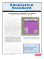
Connecting TCAD To Tapeout
A Journal for Process and Device Engineers
TCAD Simulation of a Polysilicon Thin Film Transistor
For Active Matrix Liquid Crystal Displays
1 Introduction
Polysilicon thin film transistors are attractive as active
devices in driver circuits of highly integrated active-matrix
liquid crystal displays (AMLCDs) and as p-channel metaloxide-semiconductor field effect transistors (MOSFETs) in
static random access memory (SRAM) cells.
Mobility in polysilicon is higher than that in amorphous
silicon thus enabling integration and improved performance
(e.g. high transconductance) in multi layered MOSFET
structures, and low cost AMLCDs which are becoming significantly important. As with amorphous films, polysilicon
films are granular, and as such, the grain size of the polysilicon is critical in terms of dictating electron mobility and
electrical device performance. For example several grains existing in the device channel will result in electron scattering
and electron trapping by interface and sub level traps.
Much effort has been made to increase both grain size
and mobility to promote single grain channels for the
TFT [e.g. 1]. A popular technique for promoting single
grain growth is excimer laser crystallization which is
Figure 1. Thin film device. Gate length=4μm. Device width=8μm.
now a well established technique for producing polycrystalline silicon films on non refractory substrates [2].
described the characteristics of the bandgap. However,
This is a process in which the film is nearly completely
as research continues, it is becoming important to be able
melted such that the molten grains grow laterally from
to implement density of states functions specific to the
a few isolated solid portions of seed grains that are not
device rater than general expressions that at times can
included in the molten process. In such a process grains
prove inadequate.
can have diameters far exceeding the film thickness due
to super-lateral growth phenomenon resulting in near
Continued on page 2 ...
single grain channel films [2]. However, due to complicated
growth physics and energy considerations, growth faults
will occur delivering sites which can hinder electron
INSIDE
motion and degrade device performance [e.g. 3] .
Topography Simulation of Trench Etch Using Monte
Carlo Plasma Etch Model with Polymer Re-deposition ..... 4
Of critical importance when modelling TFT devices is to
gain an accurate appreciation of these effects which are
typically manifested within the density of states in a material’s bandgap in addition to introducing grain boundary
regions within the device channel. Many density of states
functions have been proposed in the past to accurately
Volume 13, Number 11, November 2003
November 2003
Interconnect Parasitic Accuracy & Speed
Improvements in New CLEVER Release.............................8
Calendar of Events ................................................................12
Hints, Tips, and Solutions ....................................................13
Page 1
The Simulation Standard
2a Results and Discussion
A thin film transistor has been created using the ATHENA framework and is shown in Figure 1. The device
has been saved as a structure file entitled tft_device.str
with a device width of 8μm and channel length of 4μm.
In order to refine the electrical characteristics a and assign density of states to the bandgap, ATLAS has been
used. ATLAS is an intutative device simulator and an
example of some of the input deck parameters used for
this simulation is shown in Figure 2. After the initial go
atlas command, the TFT structure file is invoked using
the mesh infil=tft_device.str with the width set using
width= 8μm.
Figure 3 illustrates the density of both donor like and
acceptor like states. These profiles have been found at
this time to give the best fit to experimental data.
The C-Interpreter is invoked reference to the input deck
shown in Figure 2 using the commands f.tftdon and
f.tftacc. A simple C file has been written and saved as
defect1.c. The commands dfile= and afile= provide a
means of extracting the density profiles for the donor
and acceptor states respectively. It has been found that
for the double exponential expressions
Figure 2. Summary of input deck used.
For this study a real time polysilicon TFT device has been
developed by industrial collaborators and an attempt at
simulating its electrical performance has been undertaken
using Silvaco TCAD simulation software. The device has
undergone excimer laser crystallization and as no vertical
grain boundaries are present in the device, these have
been omitted from the simulation. However, in order to
utilize in house developed physical expressions for the
density of states, Silvaco provides a C-interpreter which
permits the user to specify specific algorithms for device
simulation which has been implemented here. In addition
to simulating the effects of density of states within the
bandgap, an attempt has also been made to include mobility
factors variable with electric field.
(1)
(2)
Figure 3. (a) Density of states for acceptor. (b) Density of states for donor.
The Simulation Standard
Page 2
the parameters to supply the best fit are shown
in Table 1. Figures 4 and 5 show the simulated
results for 0.1V and 5V on the drain contact respectively plotted on top of the experimental raw
data in each case. Clearly there is an excellent
agreement between simulated and experimental
raw data. Particular attention is now given to
the models used. To obtain such an agreement
several models have been used fundamentally
based on Fermi-Dirac statistics. Each model is
stated on the models line as shown in Figure 2.
Of particular interest is modeling the mobility of
this device. It has been found that the Lombardi
CVT model [4] invoked using cvt on the models
statement line (see Figure 2) improves the fit as
the electric field is increased. In particular the
section of this model based on the surface roughness µsr has significant effects. It has been found
November 2003
Ntail
(eV-1cm3)
Etail
(eV)
Ndeep
(eV-1cm3)
Edeep
(eV)
Donor
1.5e19
0.02
1e19
0.1
Acceptor
0.8e19
0.01
7e18
0.08
tion-recombination mechanisms occurring in the depletion region at the drain junction. At low Vds the leakage
current is dominated by thermal generation occurring in
the depletion layer close to the drain. More interestingly
however is what happens at high Vds. At high Vds, high
electric fields will be present at the drain junction and
field enhanced generation mechanisms dominate the
leakage current. Several mechanisms have been proposed
to account for this and include field enhanced thermal
emission i.e. Poole-Frenkel, trap assisted tunneling,
phonon assisted tunneling and band-to-band tunneling.
Within the TFT module it is possible to account for these
effects. For this simulation two models have been used.
These include band-to-band tunneling and band-to-band
tunneling in addition to Poole-Frenkel effect which will
be briefly be summarized. This is shown in Figure 5.
Table 1. Summarized parameter values for equations (1) and (2).
that controlling the proportional constants of the surface
roughness µsr,n and µsr,p for both the electrons and holes
respectively help to improve the simulation where:
(3)
(4)
The band-to-band tunneling effect is initiated by the bbt.std
on the models statement and it has three parameters that
the user can alter in order to better characterize a device.
If a sufficiently high electric field exists within a device
local band bending may be sufficient to permit electrons
to tunnel by field emission from the valence band into the
conduction band. To implement this effect the current continuity equations within ATLAS are altered accordingly.
The right hand side of the continuity equations are altered
by the tunneling generation rate GBBT where:
The best fit has been obtained by setting each parameter
equal to 1.65e13vs-1. An interface fixed trap density of
1.83e12 has also been used. Recombination mechanisms
used during this study are standard and include Shockley-Read-Hall (SRH) and Auger recombination. These
are implemented on the model statement as srh and
auger respectively. The carrier lifetimes have also been
specified using taun0 and taup0 for electrons and holes
respectively.
(5)
2b Effects of Band-to-Band and PooleFrenkel Tunneling
Here E is the magnitude of the electric field and BB.A,
BB.GAMMA and BB.B are user definable parameters that
can be set within the input deck. For this simulation satisfactory values have be found and are summarized in table 2.
When polysilicon TFTs are used as switching elements in
active matrices, the off current has to be low, since it limits the time the video information can remain on a pixel
before refreshing. The off current depends on the genera-
Continued on page 11 ...
Figure 4. Simulation data plotted over experimental raw data. Drain
voltage = 0.1V.
November 2003
Figure 5. Simulation data plotted over experimental raw data. Drain
voltage=5.0V. Two simulations are shown with band-to-band tunneling and with band-to-band tunneling with Poole-Frenkel effect.
Page 3
The Simulation Standard
Topography Simulation of Trench Etch Using Monte Carlo
Plasma Etch Model with Polymer Re-deposition
1. Introduction
The contribution of parallel and lateral components have
a relation to RF power and gas pressure as shown in reference [1], Figure 6.
The topography simulation module, Elite has constantly
been improved in order to simulate advanced processes,
which are becoming more complex with device miniaturization and further integration of VLSI circuits. Elite
is a two dimensional topography simulation module that
works within ATHENA, and includes the etching and
deposition models neccessary to simulate diverse modern technologies.
2-2. Reflection Ratio of Ions
The experimental depth dependent etch rate was compared to ion flux simulations in the trench. By changing
the reflection ratio of ions on the oxide wall, the relationship between the trench depth and the ion flux was
simulated. S. Takagi, et al. [1] determined that a reflection
ratio R of 0.4 showed good agreement to experimental
results, so this value was chosen as a base value.
One of the more important features of Elite , is the
physics based Monte Carlo Etch Model, which is more
accurate than conventional direction-rate based etching
models. The Monte Carlo Etch Model involves calculation of the plasma distribution, and takes into account
the redeposition of the polymer material generated as
a mixture of incoming ions and etched (sputtered) molecules of substrate material.
R=0.4 (mc.alb1 for oxide) .
2-3. Etch Rate
The etch rate is calculated with the microscopic etch rate
parameter (EtchParam) and ion velocity (see equation 2).
The perpendicular etch rate as a function of the RIE reactor conditions was reported in [1]. The details of the surface reaction model and the parameters used (including
those mentioned in section 2-2 and 2-3) will be described
in the next section.
In this article, we will discuss the relationship between
the process conditions of the reaction chamber and the
resulting etched profile. The example combines topography simulation together with plasma sheath reaction
and surface reaction modelling.
The pioneering efferts of S. Takagi, et al. [1] reported both
experimental results and plasma/topography simulation
using the ATHENA/Elite
/
/Elite
Monte Carlo Etch Model. In
this article, we are concentrating on how to specify the
many complicated simulation parameters of the Monte
Carlo Etch Model, referring to the results and calibration
work of S. Takagi, et al. [1].
EtchRate (mat) = Σ EtchParm (mat, ion) . Vabs
ion types
Eq. 2
So far we have discussed the base line physical parameters extracted from experiments in Takagi’s work [1].
The next section will discuss simulation examples using
other parameters available to the user.
3. Elementary Process of Oxide
Trench Etching
2. Simulation Model and Parameters
2-1. Incoming ions and neutrals
The procedure to specify input parameters can be broken down into the following four steps:
It is assumed that ion and neutral fluxes leaving the plasma
sheath are represented by bimaxwell velocity distribution
function [2] along the direction determined by user specified
incident angle:
step 1. Set base physical parameters refered to in the
previous section.
step 2. Tune smoothing parameters
υ||
υ⊥
||
⊥
ƒ( υ|| , υ⊥) ∼ I . exp( T − T
)
The main tuning parameter is mc.sm [3] A value of
0.1 is suggested as a starting point. The smoothness
should be tuned for the best balance of the surface
segment reaction, as shown in Figure 1, combined
with the number of particles set by mc.parts1,
mc.polympt, and mc.dt.fact. The parameter mc.dt.fact
controls etching time discretization.
Eq. 1
where v// is the ion velocity component parallel to the incident direction, v⊥ is the ion velocity component perpendicular to the incident direction, I is the ion (or neutral)
current density, T// is the dimensionless parallel temperature and T⊥ is the dimensionless lateral temperature.
The Simulation Standard
Page 4
November 2003
Plasma sheath
mc.alb1
Polymer Flux
mc.plm.alb
mc.etch1
Polymer
mat
etch
Figure 1. Surface reaction model described by tracing particles
from plasma sheath and polymer flux. Parameters depicted in
this diagram is for polymer material, which is etch/deposition
target of incident particles.
Figure 2. The result of oxide trench etch.
The three physical parameters, mc.etch1, mc.alb1, and
mc.plm.alb (seen in Figure 1) control the surface evolution in the surface reaction model [2].
3 x 3 (see Figure 1 for three materials) + 2 (Temperature of sheath) + 4 (smoothness
parameters
discussed in 2) ) = 15 .
The parameter mc.etch1 concerns the etch rate of the
particles from the plasma sheath against the respective materials, described by the right hand side of
equation 2.
The effect of polymer re-deposition could be increased either by decreasing the polymer etch rate, or
decreasing the polymer etch particle reflection from
the polymer layer (mc.plm.alb).
mc.alb1 represents the reflection ratio parameters of
the particles from the plasma sheath against the respective materials described in 2-2.
Surface evolution was calculated at the polymer etch
rate (mc.etch1=0.01e-5) 1/45 times slower than the
etch rate for oxide.
mc.plm.alb represents the reflection ratio parameters
of particles from polymer flux against the respective
materials.
In this example, the basic oxide trench was first created with a geometrical trapezoid etch which was
then followed by the second physical monte-carlo
etch. To illustrate the physical etching capabilities,
the first geometric etch left the left haand side of the
trench covered with a 10nm layer of polymer.
If an inappropriate value for the above parameters is
not specified, rough surface elements with a “zig-zag”
form will result.
Due to the intentional polymer deposition only on the
left side of the trench, an asymmetrical etch shape is
generated as shown in Figure 3. This is the effect of
the polymer re-deposition during the etching of the
trench. The extent of the asymmetry of the trench geometry depends on the polymer etch rate (mc.etch1)
and the polymer reflection (mc.plm.alb) parameters.
step 3. Further tuning of the physical parameters
Here we show an example of trench RIE simulation
to illustrate the effect of polymer growth and surface
reactions.
We consider oxide trench fabrication, and define
three rate.etch statements for oxide, resist and polymer materials respectively. There are more than 15
parameters included in these three rate.etch statements and etch statement, i.e.
November 2003
Figure 4 shows the sensitivity of the resulting etch
asymetry to the value of these parameters. The figure
illustrates a 2x2 experimental matrix of the polymer
etch rate, mc.etch 1, reflection parameters, mc.plm.alb.
Page 5
The Simulation Standard
Figure 4. Effect of redeposition comparing four different set of
parameters on symmetric/asymmetric trench geometry.
Figure 3. Overlay of geometrical trapezoid shape and subsequent two second etch
Figure 6 (Figure 13 in reference [1]) shows the etch depth
and width, respectively. The simulation reproduces
the tendencies of etch depth increasing with Rf power,
whereas etch width remains almost constant. The dependence of etch depth and width on gas pressure are
shown in Figure 7 (Figure 14 in ref [1]). The simulation
reproduces the tendencies of etch depth and width
which increase slightly with increased gas pressure.
Shown in the top left of Figure 4, the symmetry of the
bottom right trench is deeper for mc.etch1=0.01e-5
and mc.plm.alb=0.8; the top right shape is almost
symmetric for mc.etch1=0.01e-5 and mc.plm.alb=0.05
(decreased from a), but a thin polymer covers the left
side of the trench bottom.
Simulation time is less than 10 seconds for this short etch
step, with mc.patrs1=mc.polympt=10000 MC particles.
4. Process Condition Dependence
In this section we will summerize the trench etching
simulation example using the modeling parameters
discussed in the previous sections.
By using the same parameter values (except mc.etch1=0.8e-5
and mc.plm.alb=0.8) the shape of the oxide trench (shown
in Figure 5) is formed during a 1 minute etch. The value
used for polymer etch rate (mc.etch1=0.8e-5) is two times
larger than the etch rate for oxide. The ratio coresponds to
the optimized etch rate ratio against polymer and oxide,
which is compared experimentaly in [1].
Regarding simulation result dependency on the simulated process conditions, we quote two figures with the
permission of Jpn. J. Appl. Phys. These two figures compare the simulation results with experiment. RF power
and gas pressure dependency results were taken from
Takagi et al. [1].
The Simulation Standard
Figure 5. Simulated oxide trench with one minute etch using
plasma etch parameters described in secion-3.
Page 6
November 2003
Etch depth (µm)
Etch depth (µm)
0.8
0.8
0.7
0.6
Experiment
0.5
Simulation
0.4
Simulation
0.7
0.6
0.5
0.4
4
6
8
10
Gas pressure (Pa)
12
2
1
1.25
1.75
(a)
(a)
0.25
1.5
RF power (kW)
0.25
0.225
Etch width (µm)
Etch width (µm)
Experiment
0.2
0.175
Experiment
Simulation
0.15
4
6
8
10
Gas pressure (Pa)
0.225
0.2
0.15
12
Experiment
0.175
Simulation
1
1.25
1.5
1.75
RF power (kW)
(b)
(b)
Figure 6. Comparison of experimental results and simulation
results (RF power dependence):(a)etch depth, (b)etch width.
Figure 7. Comparison of experimental results and simulation results (gas pressure dependency):(a)etch depth, (b)etch width.
5. Summary
References
This article has shows the procedure to specify suitable model parameters to perform Monte Carlo plasma
etch simulations. The parameters include polymer etch
and polymer particle reflection from the polymer layer,
amongst others. It was shown that this model reproduces reasonable etching geometry. According to Takagi
et al. [1], by including plasma sheath simulations, the
relationship between the reactor conditions and model
parameters can be obtained and calibrated.
[1]
S. Takagi, et al., “Topography Simulation of Reactive Ion Etching
Combined with Plasma Simulation, Sheath Model, and Surface Reaction Model”, Jpn. J. Appl. Phys., Vol. 41 (2002), pp. 3947-3954,
Pt. 1, No. 6A,
[2] SILVACO Simulation Standard, August 1998, p6-9, “Simulating
Redeposition During Etch Using Monte Carlo Plasma Etch Model”
[3] SILVACO ATHENA User’s Manual
As for the dependence of etching profile on reactor conditions, please refer to the original paper [1].
Acknowledgment
We deeply appreciate Dr. Takagi for his essential contribution to practical application of MC Plasma Etch Model.
We also appreciate very much to Jpn. J. Appl. Phys. for
giving us permission to reprinting figures.
November 2003
Page 7
The Simulation Standard
Interconnect Parasitic Accuracy & Speed Improvements
in New CLEVER Release
Introduction
This article introduces the new features and
numerical schema implemented in the most
recent release of CLEVER from Silvaco. In
this new release, both memory handling and
simulation time are optimized to allow the
input of larger simulation structures. In addition, the release offers greater control over the
accuracy benchmarks necessary for extracted
parasitic elements.
Parasitic Extraction Accuracy
Technology
description
3D process and
device simulation
3D mesh
structure
Rule file
GDS2 layout
Netlist
extraction
Back-annotation
Accurate parasitic extraction is crucial for
deep submicron designs. Today, 3D field solvers
3D parasitic
are touted as the benchmark of accuracy, but
extraction
any field solver is only as accurate as its input
geometry. CLEVER achieves greater accuracy
by using a combination of 3D process simulation
and 3D field solver capabilities. All back end
SPICE network
Timing simulation
processes, including deposition, etching, and
with RC
parasitics
lithography, are performed before generation
Signal integrity
of the final structure geometry. This makes it
Figure 1. The parasitic extraction overview in CLEVER.
possible to obtain an accurate 3D topology of
the layout, while offering greater power and
flexibility in extracting highly accurate parasitic resisuniform criteria are used to estimate the error, the user
tances and capacitances in deep and ultra-deep submicron
will typically achieve 1% accuracy for most problems.
designs. (Figure 1)
This is because the mean error for the entire structure
is less than the specified error value. This, however, is
misleading. There is no guarantee that the user will
achieve 1% accuracy for all problems over the totality
of the 3D structure. While the software may report a
total 1% accuracy margin, this result may not be locally
applicable to the problem at hand. The additional accuracy switches solve such problems. The goal is to align
the software’s predicted error with the actual error by
adjusting the error criteria for what are very different
physical problems.
Software applications that provide numerical solutions
of real physical problems are often unable to correctly
solve all problems put to them. Adaptive solutions that
make use of user-provided tolerance specifications will
solve most problems within the specification, but overrefined problems may waste valuable computation time.
Problems that lack sufficient refinement may only appear within the user-defined tolerance specification, but
actually are not.
Silvaco has solved this problem with the introduction of
an accuracy switch in the new release of CLEVER that is
used with respect to the tolerance level required for the
parasitic extraction. The user defines the accuracy criterion. For simple problems, the user may choose to use relatively loose criteria. For difficult and complex problems,
such as designs with high interconnection density, more
rigid criteria will help to ensure an accurate output.
The ‘Adapt’ parameter defines the accuracy criteria
for both capacitors and resistors. The example below
instructs the solver to compute both extractions with a
single command:
Interconnect Adapt = (0.05 , 0.05)
The solver will then extract ALL parasitic interconnections within the user’s required 5% accuracy (the default
extractable minimum values are 0.01 Ohm for resistors
and 1E-18 F for capacitors).
Let’s illustrate with an example. If a user requires a 1%
margin of accuracy over a 3D structure, the numerical
solver should present a solution that is within that 1%. If
The Simulation Standard
Page 8
November 2003
To use these different criteria, add the following statement to the Interconnect command:
Interconnect Adapt=(0.05,0.05)
APaccuracy = tight RESaccuracy=fair
To illustrate this, we have made a 3D process simulation
of an inverter using CLEVER (Figure 2). A SPICE netlist
(Figure 3), including active devices and parasitics, was
extracted from the simulation using our 3D field solver.
We then created a SPICE input deck (Figure 4) that simulated a ring oscillator using the netlist in Figure 3.
Table 1 shows the SPICE response, memory requirements, and simulation times of a SPICE-simulated ring
oscillator based on the defined accuracy parameters. The
results indicate the computed SPICE delay, as simulated
with the parasitic netlist extracted with CLEVER, does
not vary widely in this example. However, both simulation time and memory requirements increase significantly between criteria of “veryloose” and “verytight.”
Gains can be as high as a factor of 17 for simulation time,
and a factor of 8 for memory, with a SPICE result differential of less than 2%.
Figure 2. 3D structure of an inverter.
This new version of CLEVER also offers user control
over convergence criteria in addition to the adaptive control parameter. If the accuracy requirement is loose, the
convergence is quicker. Tight requirements will slow the
convergence down.
CLEVER can also apply any accuracy criterion over a
single node. This is essential if a node is critical in the
layout design. For example, if the parasitic elements over
a node called ‘VDD’ are critical for a design, one can perform this simulation:
The five criteria for capacitance extraction are very loose,
loose, fair, tight, and very tight. The three criteria for resistance extraction are loose, fair, and tight. The default
levels for both capacitance and resistance are set to fair.
The following is an example of these parameters:
Interconnect Capacitance adapt= 0.05
Interconnect Capacitance contact=”VDD”
adapt= 0.02
RESaccuracy =tight (Resistors)
The first statement above sets the accuracy criterion to
5% over all the nodes on the circuit, while the second
Figure 3. Spice netlist
Figure 4. Spice input deck.
CAPaccuracy =tight (Capacitors)
November 2003
Page 9
The Simulation Standard
Accuracy
Simulation
Memory
SPICE delay
Switch
Time
Requirement
per stage
Very Tight
1718 s
263 Mb
46 ps
Tight
955 s
162 MB
45.89 ps
Fair
536 s
103 MB
45.78 ps
Loose
202 s
49 MB
45.52 ps
Very Loose
105 s
33 MB
45.36 ps
C1 in gnd 8.48701e-16
C1 in gnd 8.48701e-16
C2 in out 1.47932e-15
C2 in out 1.47932e-15
C3 in vdd 8.46291e-16
C3 in vdd 8.77543e-16
C4 gnd out 4.54491e-16
C4 gnd out 4.54491e-16
C5 gnd vdd 3.50237e-17
C5 gnd vdd 4.55274e-17
C6 out vdd 4.56666e-16
C6 out vdd 4.9166e-16
Default 5% accuracy
Default 5% accuracy + 2%
over VDD node
Table 1. Ring oscillator spice simulation results for different
accuracy tolerances.
Table 2. Variations in extracted capacitances when the tolerances are changed.
statement sets accuracy criterion for the specific “VDD
node” to 2%. In Figure 5, the mesh is adapted and refined
automatically within the desired 5% accuracy. In Figure
6, where the desired accuracy criterion is 2%, the “VDD
node” electrode on the left-hand side of the picture is
meshed considerably finer than in the default simulation. Since only parts of the structure are computed with
maximum accuracy, computing time is reduced. Table
2 shows that only the capacitors attached to the “VDD
node” are affected by the change in accuracy criteria.
CLEVER also includes a robust netlist reduction feature. In
the 3D structure shown in Figure 2, the gates are accessed
from the two upper metallization layers. Access resistances
must be correctly extracted and the connectivity must be
consistent. Since very small values of capacitance and resistance do not dramatically affect the SPICE simulation,
two new switches have been introduced that specify both
minimum values to be written in the SPICE netlist:
Figure 5. Default mesh (5% accuracy required).
Figure 6. Finer mesh on the VDD elelctrode (required 2% accuracy).
The Simulation Standard
Interconnect minRES= 0.01
minCAP=5E-18 Adapt = (0.05 , 0.05)
Page 10
November 2003
In this case, CLEVER performs network reduction at the
physical level of the parasitic calculation. This eliminates
direct reduction of the SPICE netlist, which could inadvertently introduce “dangling nodes.” Table 3 shows a
comparison between netlists with standard and reduced
parasitic extraction. In the reduced netlist, resistors have
been artificially limited to values above 1 Ohm. Despite
this threshold, lower values are still present in the reduced netlist in order to make sure that no dangling
nodes are introduced.
R1 aux1 gate1 49.9053
R2 aux1 i 1.11292
R3 aux1 gate0 47.805
R4 i H1 2.17512
R5 aux2 H4 0.0457013
R6 aux2 cont3 0.437311
R7 aux2 aux3 0.0556269
R8 aux3 cont5 0.4479
R9 aux3 vdd! 0.0132343
R10 aux4 aux5 0.0966024
R11 aux4 H3 0.0947903
R12 aux4 cont2 0.592232
R13 zn aux5 0.00418292
R14 aux5 cont4 0.438251
R15 aux6 aux7 0.0682582
R16 aux6 H2 0.0454305
R17 aux6 cont0 0.42867
R18 aux7 cont1 0.447886
R19 aux7 gnd! 0.0146793
Full resistors netlist
Conclusion
CLEVER 3.0.0.R release addresses the increase in complex high-accuracy circuit simulation by bringing greater attention and flexibility to accuracy handling. New
Interconnect command parameters help the user to define detailed accuracy parameters, and then to adjust the
emphasis over the numerical schema in order to tighten
or loosen convergence criteria. Memory requirements
and simulation time are lowered considerably, allowing
the input of larger, more complex structures.
R1 aux1 gate1 49.9053
R2 aux1 i 1.11292
R3 aux1 gate0 47.805
R4 i H1 2.17512
R5 cont3 H4 0.0457013
R6 cont3 cont5 0.4479
R7 cont3 vdd! 0.0132343
R8 H3 zn 0.0966024
R9 H3 cont2 0.592232
R10 zn cont4 0.438251
R11 H2 cont1 0.0682582
R12 H2 cont0 0.42867
R13 cont1 gnd! 0.0146793
Netlist reduction
Table 3. Comparison between the full resistor netlist and the
reduced resistor netlist.
...continued from page 3
3 Summary
Tunneling
Parameters
BB.A
(V/cm)
BB.GAMMA
(arb.)
BB.B
(arb.)
Initial Guess
5e20
2.0
1.6e7
A thin film transistor for active matrix liquid crystal displays
has successfully been simulated using Silvaco International’s
extensive technology computer aided design (TCAD) toolset.
It is clear that the simulation data is in excellent agreement
with experimental data from the TFT device. Accurate density
of states expressions have been presented having the form of
a double exponential expression. Poole-Frenkel in addition to
band-to-band tunneling have been demonstrated to increase
leakage current improves the fit between simulation data and
experimental data. This report was intended to demonstrate
the capability of Silvaco software in modeling thin film transistors together with demonstrating the ease of use and user
friendly approach of a complete modular system with powerful C-interpreter interface.
Table 2. Summarized parameter values for band-to-band tunneling.
The Poole Frenkel barrier lowering effect enhances the
emission rate for trap-to-band phonon assisted tunneling and pure thermal emissions at low electric fields.
The Poole-Frenkel effect occurs when the Coulombic
potential barrier is lowered sufficiently due to the electric field. The Poole-Frenkel effect is modeled by including field effect enhancement terms for Coulombic wells
and thermal emissions in the capture cross sections [5].
This model also includes the trap assisted tunneling effects in the Dirac well. This model is invoked by specifying the commands trap. tunnel and trap.coulombic
on the models statements. It can be seen from Figure 5
that by including Poole-Frenkel effects the leakage current has been increased slightly and has semblance to
the experimental data.
References
[1]
Liu G., Fonash S.J., Appl. Phys. Lett. vol. 62, p2554 (1993).
[2]
Im J.S., Kim H.J., Thompson M.O., Appl. Phys. Lett., vol. 63, p1969 (1993).
[3] Armstrong G.A., Uppal S., IEEE Trans. Electron Device letters,
EDL 18, p315 (1997).
[4] ATLAS User’s Manual Vol. I.
[5]
November 2003
Page 11
Lui O.K.B., Miglioratop., Solid state electronics, vol. 14, 4, p575 (1997).
The Simulation Standard
Calendar of Events
November
1
2
3
4
5
6
7
8
9 ICCAD - San Jose, CA
10 ICCAD - San Jose, CA
11 ICCAD - San Jose, CA
CS-MAX - San Jose, CA
12 ICCAD - San Jose, CA
CS-MAX - San Jose, CA
13 ICCAD - San Jose, CA
CS-MAX - San Jose, CA
14
15
16
17
18 EDMO - Manchester, UK
19 EDMO - Manchester, UK
20
21
22
23
24
25
26
27
28
29
30
December
1
2
3
4
5
6
7
Bulletin Board
Silvaco Acquires Simucad
ISDRS - Washington DC
ISDRS - Washington DC
ISDRS - Washington DC
IEDM - Washington DC
8 IEDM - Washington DC
9 IEDM - Washington DC
10 IEDM - Washington DC
11
12
13
14
15
16
17
18
19
20
21
22
23
24
25
26
27
28
29
30
31
Simucad Inc. is a leading provider of Verilog logic
and fault simulation software. It was founded in
1981 and has a current user base of over 9,000
design engineers. The comprehensive Silos
Simulation Environment includes an IEEE 1364
compliant Verilog simulator, graphical waveform
display, interactive debugging and analysis
tools, project management software, and analog
extensions. It will be integrated with SmartSpice
to provide a complete Mixed-Signal solution.
X-FAB Supports Silvaco
X-F
Analog/Mixed-Signal Flow
X-FAB, a leading independent mixed-signal foundry,
and Silvaco will provide mutual customers with
analog/mixed-signal process design kits that result
in higher design productivity. These kits will support
Silvaco circuit simulation and IC CAD tools on XFAB’s XC06 processes. X-FAB as a pure-play foundry
supplier specializes in the manufacturing of analog
and mixed-signal integrated circuits. The company
attaches great importance to provide their customers
with comprehensive service and first-class support
from the early product development phase through
to production.
Request for Feedback
Simulation Standard has been published
in basically the same format for over 10
years. In an effort to increase the value of
Simulation Standard to our readers, we
would appreciate your feedback on how
we can improve the publication in terms of
content, distribution or organization as we
move it from a paper document to a web
publication. We appreciate your feedback.
[email protected]
If you would like more information or to register for one of our our workshops, please check our web site at http://www.silvaco.com
The Simulation Standard, circulation 18,000 Vol. 13, No. 11, November 2003 is copyrighted by Silvaco International. If you, or someone you know wants a
subscription to this free publication, please call (408) 567-1000 (USA), (44) (1483) 401-800 (UK), (81)(45) 820-3000 (Japan), or your nearest Silvaco distributor.
Simulation Standard, TCAD Driven CAD, Virtual Wafer Fab, Analog Alliance, Legacy, ATHENA, ATLAS, MERCURY, VICTORY, VYPER, ANALOG EXPRESS,
RESILIENCE, DISCOVERY, CELEBRITY, Manufacturing Tools, Automation Tools, Interactive Tools, TonyPlot, TonyPlot3D, DeckBuild, DevEdit, DevEdit3D,
Interpreter, ATHENA Interpreter, ATLAS Interpreter, Circuit Optimizer, MaskViews, PSTATS, SSuprem3, SSuprem4, Elite, Optolith, Flash, Silicides, MC Depo/Etch,
MC Implant, S-Pisces, Blaze/Blaze3D, Device3D, TFT2D/3D, Ferro, SiGe, SiC, Laser, VCSELS, Quantum2D/3D, Luminous2D/3D, Giga2D/3D, MixedMode2D/
3D, FastBlaze, FastLargeSignal, FastMixedMode, FastGiga, FastNoise, Mocasim, Spirit, Beacon, Frontier, Clarity, Zenith, Vision, Radiant, TwinSim, , UTMOST,
UTMOST II, UTMOST III, UTMOST IV, PROMOST, SPAYN, UTMOST IV Measure, UTMOST IV Fit, UTMOST IV Spice Modeling, SmartStats, SDDL, SmartSpice,
FastSpice, Twister, Blast, MixSim, SmartLib, TestChip, Promost-Rel, RelStats, RelLib, Harm, Ranger, Ranger3D Nomad, QUEST, EXACT, CLEVER, STELLAR,
HIPEX-net, HIPEX-r, HIPEX-c, HIPEX-rc, HIPEX-crc, EM, Power, IR, SI, Timing, SN, Clock, Scholar, Expert, Savage, Scout, Dragon, Maverick, Guardian, Envoy,
LISA, ExpertViews and SFLM are trademarks of Silvaco International.
The Simulation Standard
Page 12
November 2003
Hints, Tips and Solutions
Derek Kimpton, Applications Engineer
Q. Is there a way to automatically specify mesh spacing
in ATHENA?
A. Yes, there are three ways to automatically specify
grid spacing. The most preferred method is described
below and could best be described as “semi-automatic”.
The other methods not described below utilize the
MaskViews/ATHENA interface and the adaptive meshing feature respectively.
The method described below is much preferred as it
leaves the user in complete control of the mesh. If this
simple procedure is followed correctly, mesh related
problems are much less likely to occur.
I. Introduction
(i) Mesh in the X-Direction
When deciding on the placement of mesh points in the X
direction, it is important to ensure that a defined mesh
point is placed at every etched edge or deposited edge in
the final structure.
Figure 1. Mos1ex01.str created using the preferred method for automated mesh spacing in the X-direction
If there is a vertical edge in the structure in a location without a corresponding mesh point, the meshing algorithum
then has to re-arrange the mesh to ensure that one exists.
During the re-arrangement process, X-mesh points near
the effected surface may have to be removed to create the
new mesh. Usually this is fine if it happens only once or
twice, but if it happens repeatedly, the user is no longer in
control of the mesh locations in the X-direction.
single oxidation can require numerous internal re-meshing events as the oxide front advances. Needless to say,
if process steps such as repeated HF dips make little
difference to the final structure (even though they are
necessary in reality), they are best left out.
(ii) Mesh in the Y-direction
In common with meshing in the X-direction, Y-direction
meshing should also ensure a Y-mesh point at each etch depth
to reduce the occurance of automated re-meshing events. Y
meshing definition should also ensure that sufficient meshing
is provided to accurately reflect each implanted profile.
The meshing algorithum does not know in advance, what
the next process step is going to be. Thus the automated
re-meshing algorithum may remove X-mesh points that
it will require for a later process step, necessatating further automated mesh re-generation. Eventually, if this
situation happens repeatedly, the mesh becomes dis-ordered and structural problems become more likely.
II. The Preferred Method for Automated
Mesh Spacing
The preferred method for automated mesh spacing requires the user to look through all the processing steps
in the input file where etching events occur. Then ensure
an X and Y point is defined for these points. X points are
easy to define, but Y points may need to be calculated if
non absolute coordinates are used in the etch statement.
For example, using the statement:
Examples of process events that are likely to cause mesh
problems due to the effects described above are repeated
oxidizing anneals, followed by HF dips or etches which
generally occurs in silicon processing. Each time a
vertical edge is oxidized, the silicon vertical edge location is shifted, necessatating an automated re-meshing.
Repeated oxidation and etching can therefore require
numerous automated mesh re-arrangements. In fact, a
November 2003
etch silicon dry thick=0.1
Page 13
The Simulation Standard
requires the user to know the original height of the relevant part of the structure being etched.
In order to illustrate how to create a minimum structure
mesh in the X-direction, let us use mos1ex01 as an example. Looking through the input file, it will be noticed
that there are etch events at X=0.18, X=0.2 and X=0.35.
Using just these locations and adding the locations of
the structure edges, we could create an automated grid
spacing in the X-direction using the following syntax:go athena
line x loc=0
line x loc=0.18
line x loc=0.2
line x loc=0.35
line x loc=0.6
Notice how the usual “spac=<value>” parameter after
all the “line x” statements is absent, instructing Athena
to choose a suitable value automatically.
Figure 2. Mos1ex01.str created by manually modifying only the Xspacing at the poly gate edge and leaving all other automatic
Since there are no critical Y-direction etching events in
this example, such as trench etches, the Y mesh points
can be left as is for this illustration, but the same techniques can be applied if required.
values by 2, so the real spacing specified by “line x
loc=0.35 spac=0.005” is actually 0.01 microns and not
0.005 microns. The automated spacing feature accessed
by removing the “spac” parameter is uneffected by
space.mult in the init statement.
If all the “line x” statements of mos1ex01.in are replaced
with this new automated mesh spacing syntax, the
mesh created is shown in Figure 1.
A further advantage of the meshing method described
above is that if the user is simulating a set of similar
structures, such as simulating identical MOS devices
with differnt gate lengths, the “set” statement can be
used to define critical dimensions such as the X-location
of the poly gate edge. If the same variable name is used
to define this location in the mesh statement the meshing can remain automatic for each input file, even when
the gate length changes.
This will provide a good basic mesh which will run
fast due to it’s minimilist nature and show any errors
in process statements. Let’s say that the process part
is now de-bugged and the user now wishes to increase
the number of mesh point around the edge of the poly
gate to get an accurate result for the final run. The Xmesh statements could be modified by simply adding
one spacing value at the poly gate edge (X=0.35um) as
follows:go athena
line x loc=0
line x loc=0.18
line x loc=0.2
line x loc=0.35 spac=0.005
line x loc=0.6
Call for Questions
If you have hints, tips, solutions or questions to contribute,
please contact our Applications and Support Department
Phone: (408) 567-1000
Fax: (408) 496-6080
e-mail: [email protected]
In this instance, only the X-location corresponding to the
edge of the poly gate was manually modified. The final
mesh is now shown in Figure 2. It is important to note
here that in mos2ex01.in, the “space.mult=2” parameter
in the “init” statement multplies all “spac=<number>”
The Simulation Standard
Hints, Tips and Solutions Archive
Check our our Web Page to see more details of this example
plus an archive of previous Hints, Tips, and Solutions
www.silvaco.com
Page 14
November 2003
Contacts:
Silvaco Japan
[email protected]
Silvaco Korea
[email protected]
USA Headquarters:
Silvaco Taiwan
[email protected]
Silvaco International
4701 Patrick Henry Drive, Bldg. 2
Santa Clara, CA 95054 USA
Silvaco Singapore
[email protected]
Silvaco UK
[email protected]
Phone: 408-567-1000
Fax: 408-496-6080
Silvaco France
[email protected]
[email protected]
www.silvaco.com
Silvaco Germany
[email protected]
Products Licensed through Silvaco or e*ECAD
November 2003
Page 15
The Simulation Standard