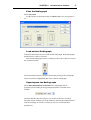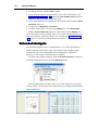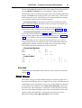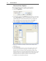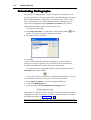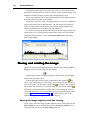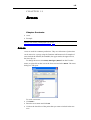
1
Viewbox
V
E
R
S
I
O
N
3.1.1
Viewbox version 3.1.1
Manual version 3.1.1.0
Copyright © Demetrios J. Halazonetis, Kifissia, Hellas (Greece), 1995-2003.
All rights reserved.
No part of this manual may be reproduced or transmitted in any form or by
any means and for any purpose without the written permission of the author.
Microsoft Windows, Microsoft Excel, Microsoft Word and Microsoft
PowerPoint are registered trademarks of Microsoft Corporation.
Demetrios J. Halazonetis,
6 Menandrou Street,
Kifissia 145 61,
Hellas (Greece)
Fax: +30-210-623.3211
E-mail: [email protected]
Web site: www.dhal.com
iii
Table of Contents
INTRODUCTION TO VIEWBOX
Introduction
Capabilities and Limitations
Installation
Basic Concepts
Screen Layout
Short Tutorial
The Current, Reference and Morph Source
LOADING, SAVING AND DELETING RADIOGRAPHS
Radiograph Files
Loading a Radiograph
Saving a Radiograph
Replacing a Radiograph
Changing the Radiograph File
Deleting a Radiograph
Organizing Your Radiographs
File Format of Radiograph Files
VIEWING RADIOGRAPHS
Viewing and Zooming
Life Size
Grid
Colors and Lines
ANALYZING RADIOGRAPHS
Tracing Analysis
Tracing Analysis Options
Deviation from Mean
Font
Text Analysis
Text Analysis Options
Show Normal Values
Show Graph
Styles
Extended Analysis
Extended Analysis Options
Customizing the Extended Analysis
Measuring Manually
Ruler
Protractor
PRINTING AND COPYING RADIOGRAPHS
The Print Dialog Box
Tracing
9
9
10
10
11
12
13
18
19
19
20
22
23
24
24
24
25
27
27
29
30
31
33
33
34
34
35
35
37
37
37
37
38
39
39
44
44
45
47
47
48
iv
Viewbox Manual
Text
Extended
Print Areas
Printing Options
Quick Print
Copy to Clipboard
Pasting to Other Programs
Save as Metafile
Export Image
Save Results
Send To
49
51
51
52
52
52
53
54
54
54
55
DIGITIZING RADIOGRAPHS
57
Introduction
Orientation cursor
Auto edge-locking
Snakes
Creating a New Radiograph
Digitizing
Digitizing with a Digitizer
Digitizing on Screen
The Digitize Dialog
Points without Auto edge-locking
Points with Auto edge-locking
Snakes
Notes on Digitizing
Redigitize
Digitizing Options
Image Size
Default Image Directory
Digitizer Setup
Magnification tool
57
58
58
58
59
60
60
60
61
62
63
65
67
68
69
69
71
71
76
EDITING RADIOGRAPHS
79
Introduction
Selecting Areas and Points
Translating
Rotating
The Movement Window
Some Quick Ways to Move
Auto VTO
Other Functions
Scale
Flip Vertical, Flip Horizontal
Get Coordinates From
79
79
81
83
86
88
90
91
91
91
92
SUPERIMPOSING AND ORIENTATING RADIOGRAPHS
Superimposing Radiographs
Orientating Radiographs
IMAGE FUNCTIONS
Introduction
93
93
94
95
95
v
Image Functions
Levels
Moving and rotating the image
Moving the image together with the tracing
The Image Position / Rotation box
Image rotation with resampling
Image transparency
Align Tracing with Image
Morphing - Warping
Interactive Morphing
EXPORTING ANALYSIS RESULTS
Introduction
Exporting Results
Notes on Using Other Programs
MEAN RADIOGRAPH
Introduction
Calculating the Mean
Notes on the Mean Procedure
SORT BY SHAPE
Introduction
Sort by Shape
PROCRUSTES AND PCA
Introduction
Details
RADIOGRAPH TYPES
Introduction
Opening and Creating a Radiograph Type
RADIOGRAPH TYPE NAME AND IMAGE
Radiograph Type Properties
Example
DIGITIZED POINTS
Digitized Points
Types of Digitized Points
Edge Locking
Example
SNAKES
Snakes
DERIVED POINTS
Derived Points
Types of Derived Points
Example
AREAS
95
97
98
98
99
99
99
100
103
105
107
107
107
109
111
111
111
112
115
115
115
117
117
117
119
119
122
125
125
126
129
129
130
132
134
137
137
139
139
140
143
145
Areas
Example
145
146
GRAPHICS
149
vi
Viewbox Manual
Graphics
Graphic Types
Graphic Attributes
Example 1
Example 2
Example 3 - Left Facing View
VARIABLES
Variables
Variable Types
Variable Attributes
Normal Values
Example
ANALYSES
Analyses
Analysis Attributes
Example
SUPERIMPOSITIONS
Superimpositions
Superimposition Types
Example
ORIENTATIONS
Orientations
Orientation Types
Options
Example
PROTOCOLS
Protocols
Protocol Attributes
Example 1
Example 2
VTO RELATIONSHIPS
VTO Relationships
VTO Relationship Attributes
VIEWS
Views
View Attributes
PRINCIPAL COMPONENT ANALYSES (PCAS)
PCAs
149
150
154
155
156
156
159
159
160
164
165
166
169
169
170
171
173
173
173
175
177
177
178
179
179
181
181
182
182
183
185
185
186
189
189
189
191
191
VIEWBOX INITIALIZATION FILE
193
PASSWORDS AND PERMISSIONS
199
VIEWBOX MESSAGES
201
COMPATIBILITY WITH EARLIER VERSIONS
209
LATERAL CEPH DEFINITION FILE
211
FRONTAL CEPH DEFINITION FILE
219
vii
DENTAL CASTS DEFINITION FILE
223
9
CHAPTER 1
Introduction to Viewbox
Chapter Contents:
•
•
•
•
•
•
Introduction
Capabilities and Limitations
Installation
Basic Concepts
Screen Layout
Short Tutorial
Introduction
Viewbox was designed as a cephalometric analysis program. It was
developed by an orthodontist during the period of many years. Initially it was
written for personal computers in the DOS environment and later it was
ported to Windows 3.1. The early versions were shareware. Version 2.60 was
completely re-written and major enhancements were introduced. Version
3.1.1 incorporates the latest in cephalometric analysis software, including
advanced image processing algorithms, Procrustes superimposition and
Principal Component Analysis. We believe that Viewbox can satisfy all your
cephalometric analysis needs. However, we also believe that there is always
room for improvements and we would appreciate any comments or
suggestions that you might have.
Special provisions have been taken to ensure that Viewbox can perform
any analysis that you may be using today and probably any that you might be
using in the future. Viewbox is not restricted to cephalometric analyses,
however. You can customize Viewbox yourself and perform measurements on
any diagnostic record that can be placed on a digitizer, scanned with a
scanner or photographed with a video or digital camera. Such records might
include frontal, submentovertex and panoramic radiographs, orthodontic
models, facial and profile photographs, hand-wrist radiographs, animal
radiographs, etc. Therefore, in addition to clinical diagnosis, Viewbox is
especially suited for research projects.
10
Viewbox Manual
Capabilities and Limitations
Viewbox capabilities are so numerous that the only way to appreciate them is
to use the program yourself. Only some of the strong points can be mentioned
here:
• Complete customization of points, measurements, tracing and analyses.
• Advanced image-processing filters for enhancing quality of scanned
radiographs.
• Edge locking, for automatically identifying hard/soft tissue boundaries.
• Automatic location of points along skeletal contours.
• Superimposition of up to ten radiographs of the same or different patients.
Procrustes superimposition.
• Principal component analysis for morphometric assessment of shape.
• Treatment prediction by movement of skeletal and dental units.
• Multiple Undo and Redo feature.
• Automatic soft tissue adaptation to hard tissue movements (user
definable).
• Morphing of photographs for photorealistic prediction of treatment
outcome.
• Calculation of the 'mean' radiograph of a sample.
• Export of measurements for statistical processing.
• Redigitizing feature for adding or editing points.
Because Viewbox was designed as a diagnostic tool, some facilities that are
seen in programs related to patient education and marketing are not included.
Thus, although you can simulate orthodontic and surgical treatments
manually, Viewbox does not include an automated growth or treatment
prediction.
Installation
To install Viewbox follow these steps:
Make sure that your computer is running Microsoft Windows 98SE/ME or
Windows NT/XP.
Insert the Viewbox CD-ROM. The Viewbox installation program should
start automatically. Follow the directions for installing Viewbox.
If the installation program does not start automatically when you insert the
CD-ROM, then use the Windows Explorer to run the SETUP.EXE file.
Note: If you are using Windows XP or NT, you must be logged on as an
administrator. The installation program will notify you, if this is not the case.
If you are upgrading from a previous version:
Version 3.1.1 will install over a previous Viewbox 3 version. When
installing, select the upgrade option, so that your settings and radiograph type
files are not overwritten. However, it is strongly recommended to backup
your files before installation.
CHAPTER 1 Introduction to Viewbox
11
Note: Radiographs saved with version 3.1.1 cannot be opened by previous versions,
because the new version additionally saves information related to image rotation.
To un-install:
• Select Start | Settings | Control Panel from the Taskbar.
• Open the Add/Remove Programs applet by double-clicking on it.
• Select Viewbox 3 in the list and click the Add/Remove... button.
Before un-installing, it is recommended that you keep a copy of your
radiograph files (*.CSV and *.VBR files).
The first time that Viewbox is run it will ask for your registration Key. The
registration key is specific to your computer and can be obtained by sending
us the Code number that appears in the registration dialog box. If you install
Viewbox on more than one computer in your office or home, you will need to
send a registration code for each computer. If you upgrade your computer in
the future, Viewbox may again ask for a registration key. Please note that you
can fully use Viewbox even before you send for your registration key, but you
will be continually prompted for it.
Note: If you have upgraded from a previous version and have kept the Viewbox
Initialization file during installation, as mentioned above, you do not need to get a
new Key.
Basic Concepts
Viewbox is not hard-wired to perform a pre-defined set of cephalometric
analyses. Actually, no cephalometric information has been programmed in
Viewbox. Viewbox does not have any knowledge of what a lateral
cephalogram is, which angle ANB is, or what Steiner's analysis is. All the
information regarding the cephalometric points, measurements, analyses,
superimpositions etc. is contained in Radiograph Definition files, which
reside in your hard disk (these files are named with a VBR extension, e.g.
‘lateral.vbr’). Each time Viewbox needs to analyze a radiograph, it reads the
information from the appropriate file. This gives Viewbox amazing flexibility
because Radiograph Definition files can be created and changed by the
orthodontist.
You can have as many Radiograph Definition files as you like. Each will
correspond to a different radiograph kind (or other diagnostic record). For
example, you may have a Radiograph Definition file for lateral cephs,
another for frontal cephs and another for submentovertex radiographs. Each
time you digitize a radiograph you need to let Viewbox know what kind of
radiograph it is. Viewbox will then read the necessary information from the
corresponding Radiograph Definition file and perform the correct analysis.
Each Radiograph Definition file describes a Radiograph Type. Radiograph
Types are the various orthodontic records that can be used with Viewbox,
such as the lateral ceph, the frontal ceph, the panoramic, etc. The term
12
Viewbox Manual
'Radiograph Type' does not refer to a particular radiograph of a specific
patient, but to the concept of the Lateral Ceph, or the Frontal Ceph, etc.
Radiograph Definition files contain information that describes the
characteristics of each Radiograph Type, e.g. the names of the cephalometric
points, the measurements and their normal values, the analyses, the
superimpositions that can be performed, etc.
A Radiograph is a particular instance of a Radiograph Type, i.e. it is a
specific radiograph of a specific patient. Radiographs are stored in
Radiograph files (these files are named with a CSV extension, e.g.
‘patient.csv’). Radiograph files contain only information specific to
Radiographs themselves, such as the name of the patient, the date the
radiograph was taken, the Type of the radiograph and the positions
(coordinates) of the cephalometric points that have been digitized. You can
have as many radiograph files as you wish. The number of radiographs that
each radiograph file can hold is only limited by the capacity of your hard
disk.
Viewbox can hold and show on the screen up to ten radiographs at the
same time. These may be of different patients and different types. The
tracings of all radiographs may be visible but the cephalometric
measurements are shown only for one. This is called the 'current' radiograph.
Screen Layout
The Viewbox window is divided into four main parts, as shown below:
The Toolbars are used to gain access to some of the most commonly used
commands and to the various 'tools' used for performing a VTO (Visual
Treatment Objective). A section of the Toolbar containing buttons for the
main commands and the tools used for VTO can be detached and used as
free-floating windows. To detach a Toolbar, position the mouse on the
vertical bars on the left side of the Toolbar, depress the left mouse button and
CHAPTER 1 Introduction to Viewbox
13
drag the mouse away from the Toolbar. The floating toolbar can be
reattached, by dragging it onto the Toolbar area.
The Icon Area shows one icon for each radiograph that has been loaded
into Viewbox. If more than one radiographs are loaded, the current
radiograph is the one with its label highlighted. Up to 10 radiographs can be
loaded.
The Display shows the tracing of the radiographs and the results of the
cephalometric analyses. When you first start Viewbox the Display will be
empty. The previous figure shows the Display after one radiograph has been
loaded.
The Status Bar shows helpful information, depending on the command
being executed. The Status Bar is divided into four sections. The sections,
from left to right, display the following:
• Hints related to various menu commands, results of measurements after
using the Ruler and Protractor (see Extended Analysis, p.37), and
distances that an area was translated or rotated (see Editing Radiographs,
p.79).
• The area that is currently selected (see Editing Radiographs, p.79).
• The status of the Auto Scale to Life Size feature (see Life Size, p.29).
• The coordinates of the mouse pointer.
Short Tutorial
To introduce yourself to the way Viewbox works, please follow the steps
described below. This short tutorial aims to give you a quick overview of the
basic features of Viewbox. Detailed explanations can be found in the
following chapters of this manual. It is assumed that you have already
installed Viewbox.
Load a Radiograph
Select File | Open... or click on the Open icon in the Toolbar:
The Load Radiographs dialog box will appear:
14
Viewbox Manual
Select any patient and click the Load and Exit button:
Alternatively, double-click on any name.
The tracing, together with the associated cephalometric radiograph, will
be loaded into the Display.
Display the Analysis
Select an analysis from the Toolbar:
The results of the cephalometric analysis should be visible in the Display. If
not, select View | Analysis or click the Analysis button on the Toolbar:
Values that are green are within one standard deviation from the normal mean
value. Blue values are more than one standard deviation from the mean.
Magenta values are more than two standard deviations and red values are
more than three standard deviations from the mean.
Display the Text Analysis
Select the first entry of the Windows menu. The Text Analysis window will
open, containing the detailed results of the cephalometric analysis:
CHAPTER 1 Introduction to Viewbox
15
Upright Lower Incisor
Select the Select Area (or Chooser) tool from the Toolbar:
Click near the lower incisor tip, or the lower incisor apex, to select the tooth:
Select the Rotation Center tool from the Toolbar:
Click near the center of the lower incisor root to position the Rotation Center:
16
Viewbox Manual
Select the Rotation tool from the Toolbar:
Position the mouse cursor anywhere on the tracing (but not on any of the
point markers) and drag the mouse so that the lower incisor tips labially:
The analysis results will update automatically as you move the mouse.
Select Edit | Undo to undo the movement and return the incisor to its
previous position. Now click on the Auto VTO button so that it becomes
depressed:
Rotate the incisor again and notice how the lower lip also moves as you tip
the incisor forward:
Save the Radiograph
Select File | Properties to open the Properties dialog box.
Change the Comments to ‘Ortho prediction’:
Click OK.
Select File | Save or click the Save button on the Toolbar:
The changed radiograph has now been added to the 'sample.csv' file. The
original radiograph has been retained.
CHAPTER 1 Introduction to Viewbox
17
Print the Radiograph
Select File | Print.
Set the options as shown here and click Print. Make sure your printer is
on.
Load another Radiograph
Follow the instructions above to load another radiograph. Both radiographs
should now be visible in Viewbox.
Select each radiograph in turn by clicking on the icons in the Icon Area of
the Viewbox window:
The measurements that are shown in the Display belong to the radiograph
whose icon label is highlighted (this is the 'current' radiograph).
Superimpose the Radiographs
Select Edit | Superimpose on Current. The radiographs will be
superimposed according to the superimposition that is selected in the
Toolbar:
We hope that this short tutorial gave you an idea of the basic Viewbox
functions. Please read the rest of the manual to become thoroughly familiar
with the workings of Viewbox, so that you can use it efficiently and
productively.
18
Viewbox Manual
The Current, Reference and Morph Source
Viewbox can hold up to ten radiographs in the Icon Area. Of these, the
selected radiograph is the one with its title highlighted. This is called the
Current radiograph and it is the radiograph on which all the functions are
performed (movements, analyses, saving, printing, etc.). Some Viewbox
functions require a second radiograph to be loaded. For example, when doing
a morphing of an image, Viewbox creates a morphed picture from the image
of a source radiograph. The radiograph used as a source for morphing is
called the Morph Source. Additionally, a second radiograph can be used as a
reference for performing inter-radiograph measurements, i.e. measurements
that involve two radiographs, or for transferring coordinates from one
radiograph to another. This radiograph is called the Reference radiograph.
You can specify which radiograph is the Morph Source and which radiograph
is the Reference radiograph by using the menu that pops-up when you rightclick on the radiograph’s icon in the Icon Area:
The Reference radiograph and the Morph Source are marked by a small icon,
as shown below. In this example, the topmost radiograph is the Morph
Source, the middle radiograph is the current radiograph and the bottommost
radiograph is the Reference radiograph:
19
CHAPTER 2
Loading, Saving and
Deleting Radio
Radiographs
Chapter Contents:
•
•
•
•
•
•
Radiograph Files
Loading a Radiograph
Saving a Radiograph
Deleting a Radiograph
Organizing Your Radiographs
File Format of Radiograph Files
Radiograph Files
Viewbox saves your radiographs in files that are called Radiograph files.
Each Radiograph file can hold a large number of radiographs that may belong
to the same or to different patients. The radiographs may also be of different
types. For example, you can store lateral cephalograms, frontal cephalograms
and panoramic radiographs in the same file.
A Radiograph file contains the following information for each radiograph that
is saved:
• Name of Patient
• Date of Birth
• Sex of Patient
• Date that the radiograph was taken (Date Taken)
• Magnification factor of radiograph
• Comments
• Type of radiograph
• File name of the associated image (if available) and information about the
image’s position, scaling and rotation.
• Coordinates of digitized points
Name of Patient
This can be any sequence of up to 30 characters or numbers, but commas are
not allowed. Viewbox does not differentiate between first and last name.
20
Viewbox Manual
Sex of Patient
An "F" is written to the file if the patient is female and an "M" if the patient
is male.
Date of Birth - Date Taken
These dates are used to calculate the patient's age at the time the radiograph
was taken. The dates are always saved in the day/month/year format, but will
be displayed in Viewbox according to your Windows Regional settings.
Magnification
Viewbox stores the magnification factor of each radiograph, so that you can
compare and superimpose radiographs of different magnifications, and derive
your measurements based on the patient's true size.
Comments
Any comments or notes about the radiograph. Can be any sequence of
characters (except commas) up to 30 in length.
Type of Radiograph
The radiograph's Type, e.g. Lateral ceph, Panoramic, etc.
Image data
The file name of the associated image, and data related to the image’s
position, scaling and rotation. The associated image is an image that is
automatically loaded when the tracing is loaded. It is usually the original
image that was digitized on-screen.
Point Coordinates
The coordinates of all digitized points are saved, separated by commas. For
each point the x- and y-coordinates are saved. If a point has not been
digitized, then that point is saved as "nil, nil".
You can have many Radiograph files in your hard disk. You are free to name
these as you wish, but all Radiograph files must have ".CSV" as an extension.
This extension may not be visible in Windows Explorer. If you want to see
the ".CSV" extension when you use Explorer, select View | Folder Options...
from Explorer's menu and make sure that Hide file extensions for known
file types is not checked:
Note: Windows Explorer may report that .csv files belong to a different program
than Viewbox, e.g. they may be described as "Microsoft Excel Comma Separated
Values Files". This does not affect the way Viewbox works and can be ignored.
Loading a Radiograph
To load a radiograph from your disk select File | Open... or click on the Open
icon in the Toolbar:
CHAPTER 2 Loading, Saving and Deleting Radiographs
21
The Load Radiographs dialog box will open:
Each line represents one radiograph. The name of the patient is shown,
followed by the date the radiograph was taken, the type of the radiograph and
the comments. The name of the associated image file (if any) follows. The
width of each of the five columns (name, date, type, comments, image) can
be adjusted by dragging the border of the column with the mouse. The
radiographs are shown either sorted by Name (if the Options | Sort by Name
menu item is checked), or, in sequence according to the date that they were
saved (more recent radiographs are at the bottom of the list).
To load a single radiograph:
• Select the radiograph from the list.
• Click Load and Exit
or
• Double-click the desired radiograph.
To load more than one radiograph:
• Select the desired radiographs by holding down the Ctrl key and clicking
on them
or
• Select one radiograph and then click on another radiograph while pressing
the Shift key. All radiographs between the first and second will be
selected.
• Click Load and Exit.
To load all radiographs of a specific patient:
• Select any radiograph of the desired patient.
• Click Edit | Expand Selection
• Click Load and Exit.
If you don’t want to load the image:
To stop Viewbox from loading the associated image, make sure that the
Load Image button is not depressed
.
22
Viewbox Manual
If the Radiograph file contains many radiographs and it is not easy to find the
desired ones, you may instruct Viewbox to display only a subset of them. For
example:
To show only those radiographs belonging to patients
named "John":
• Open the Filter area, by Options | Show / Hide Filter menu command, or
by clicking the Filter button
• The filter area will appear:
• Enter John in the Show only those containing: box.
• Select Name in the In field: list box.
• Click Apply.
Note: Viewbox has room for up to 10 radiographs. If you attempt to load more than
10, or there are already some radiographs loaded and you attempt to load more
than can fit, Viewbox will load as many as possible and ignore the rest.
Note: If you want to load radiographs from another Radiograph File, then click the
Open button
and select the desired file.
Saving a Radiograph
To save a radiograph to your disk select File | Save or click on the Save icon
in the Toolbar:
The Radiograph file into which the radiograph will be saved depends on the
following:
• If the radiograph was loaded from a Radiograph File, the same file will be
used to save it.
CHAPTER 2 Loading, Saving and Deleting Radiographs
23
• If the radiograph is a new radiograph that has just been created and
digitized, it will be saved in the default Radiograph file. The default
Radiograph file is shown in the New Radiograph dialog box that opens
when a new radiograph is created (see Creating a New Radiograph, p.59).
To save the radiograph into a different radiograph file from the one it was
loaded from, select File | Save Into...
To save all loaded radiographs, select File | Save All.
Replacing a Radiograph
When you save a radiograph to a Radiograph file, Viewbox will first check
that the same radiograph is not already in the file. Viewbox compares the
Name, Date of Birth, Sex, Date Taken, Magnification, Comments and Type of
each radiograph in the file to the corresponding data of the radiograph to be
saved.
• If a match is not found, Viewbox will save the radiograph to the end of the
file.
• If a match is found, Viewbox will ask to replace the radiograph in the file:
• Click Yes if you want to erase the radiograph in the file and replace it
with the new radiograph. The only difference between the radiographs
will be in the coordinates of the points.
• Click No to abort the Save procedure.
Be careful when performing treatment predictions. If you load an original
radiograph, then do the prediction and attempt to save your treatment
prediction, Viewbox will offer to replace the original radiograph with the
prediction. If you consent, you will lose your original radiograph. To keep
both radiographs, change the Properties of the prediction before saving it:
• Select File | Properties...
• Change the Comments of your radiograph to something like "4 premolars
prediction".
• Save the radiograph.
Because the original and prediction radiographs will now have the
Comments different, Viewbox will append the prediction radiograph to the
file, instead of replacing the original radiograph.
24
Viewbox Manual
Note: The Duplicate command may be helpful in such situations. Before starting a
prediction VTO, you can use the Edit | Duplicate command to create a duplicate of
the current radiograph. As soon as the duplicate is created, the Properties dialog
box will open and you can change the Comments (e.g. “Prediction tracing”). Then,
do the VTO on the duplicate.
Changing the Radiograph File
Every time a radiograph is loaded, it carries with it the name of the
originating file. This name is used by Viewbox to save the radiograph back to
the same file from which it was loaded. The name of the file can be seen in
the Properties box, opened by selecting File | Properties...
Click File... if you want to change the Radiograph file to a different one.
To change the default Radiograph file that Viewbox uses for all new
radiographs you have to open the Options dialog box:
• Select Options | Options...
• Click on the General tab
• Click on Save File...
• Select the desired file, or enter a name for a new file.
• Click OK
Viewbox will remember the new setting the next time you use it.
Deleting a Radiograph
Deleting a radiograph is performed from the Load Radiographs dialog box.
.
Just select the desired radiographs and click the Delete button
The radiographs that are deleted are deleted permanently and cannot be
recovered. Use this feature with caution.
Organizing Your Radiographs
Although you can keep all your radiographs in one Radiograph file, this may
grow too large and make it difficult for you to access your radiographs. It is,
therefore, recommended to have a system to organize your radiographs for
easy reference. Here are a couple of ways to do it:
Save each radiograph in a different file depending on
the last name initial of the patient:
For example, you can have the following Radiograph files:
A-D.csv
E-H.csv
CHAPTER 2 Loading, Saving and Deleting Radiographs
25
I-L.csv, etc.
This allows you to easily locate a patient by last name. However, it is difficult
to find radiographs according to type (lateral, frontal, etc.) or malocclusion
(Class I, Class II, etc.).
Classify radiographs according to malocclusion:
For example, you can use Radiograph files such as:
ClassI.csv
ClassII.csv
OpenBite.csv, etc.
This may cause you difficulties if you do not remember the malocclusion of a
patient, or if it is possible to classify a patient to more than one category (i.e.
Class II, open bite).
You could also use both methods and double-save each radiograph.
e Format of Radiograph Files
File
Fil
You do not need to understand the file format of the Radiograph files in order
to use Viewbox. This information is provided for experienced computer users
only.
Radiograph files (.csv) are pure text files and can be opened with any text
editor (i.e. Notepad) or word processor. Each radiograph is saved as a single
line of text ending with a carriage return - line feed character. The data
consists of the following fields:
• Name of Patient: a string of 30 characters
• Date of Birth: a string of 10 characters representing the patient's date of
birth.
• Patient's sex: An 'M' or 'F' depending on the patient's sex.
• Date Taken: a string of 10 characters representing the date the radiograph
was taken.
• Magnification: The magnification factor of the radiograph. A string of 5
characters.
• Comments: The radiograph's comments. A string of 30 characters.
• Type: The radiograph's type. A string of 20 characters.
• Associated image: The file name of the associated image (if any) enclosed
in double quotes, preceded by the angle of image rotation (in radians) and
followed by position and scaling coordinates.
The above data are separated by commas and are followed by the x- and ycoordinates of all digitized points. The coordinates of points that have been
skipped during digitization are written as 'nil, nil'. If the information that is
written to each field is smaller than the length of the field, it is padded with
'space' characters.
For example:
26
Viewbox Manual
Mary•Jones••••••••••••••••••••,5/6/1982••,F,6/8/1994••,
10•••,Pretreatment••••••••••••••••••,Lateral•ceph••••••••
,0.24,"\091016\091016_ceph_18-3-91.jpg",0,0,1.693,1.693,
1456.697,345.029,2154.921,136.393,2244.662,652.149,2237.0
49,1015.108,nil,nil
Spaces (shown here with a dot to make them visible) are necessary for
Viewbox to read the file. The above example is printed here in five lines but
occupies a single line in the file and has a carriage return - line feed sequence
at the end. All decimal numbers are written using the ‘.’ (dot) decimal
character, irrespective of the decimal separator character that is set in the
Windows Control Panel.
You can edit radiograph files using Notepad, but this is not recommended
because you may accidentally corrupt the file. Radiograph files can also be
opened by Microsoft Excel. However, the trailing spaces are not retained and
the file will be unreadable by Viewbox if it is saved by Microsoft Excel.
27
CHAPTER 3
Viewing Radiographs
Chapter Contents:
•
•
•
•
Viewing and Zooming
Life Size
Grid
Colors and Lines
Viewing and Zooming
A radiograph that has been loaded into Viewbox is represented by an icon in
the Icon Area. Viewbox can hold up to ten radiographs at the same time. The
tracing of each radiograph is normally shown in the Display. If you have
loaded more than one radiograph, the Display may become cluttered with the
tracing of each radiograph. In such a case it may be preferable to show only a
few radiographs and hide the rest.
To hide a tracing of a radiograph:
Select View | In View from the main menu or from the menu that pops-up
when you right-click on the icon of a radiograph in the Icon Area, or,
use the View button next to the radiograph’s icon:
The tracing of this radiograph is visible. Clicking the left arrow will hide it.
To show a tracing of a radiograph that has been
hidden:
Select View | In View again, or,
use the View button next to the radiograph’s icon:
The tracing of this radiograph is not visible. Clicking the right arrow will make it visible.
Sometimes you may wish to see only part of the tracing. For example, if you
are superimposing two radiographs on the mandible, you may wish to see
28
Viewbox Manual
only the mandibles. To show only part of the tracing, select the desired part
from the View list box on the toolbar:
or, from the menu that pops-up when you right-click on the View button:
Viewbox supports various methods to zoom-in or zoom-out on part of a
tracing.
To zoom in or out so that the tracing of the current
radiograph fits the dimensions of the Viewbox window:
at the
Select View | Best Fit from the menu, or click on the Best Fit icon
lower right of the Display, or select Best Fit from the zoom list box in the
Toolbar:
To zoom to a specific zoom factor:
Select a pre-defined zoom factor from the zoom list box in the Toolbar or
enter the desired zoom factor using the keyboard and press Enter.
To zoom-in or zoom-out:
Select View | Zoom In or View | Zoom Out from the menu. The zoom factor
will increase or decrease according to the pre-defined zoom factors.
Alternatively:
• Select the Zoom tool on the Toolbar:
• The mouse cursor will change into a magnifying lens:
CHAPTER 3 Viewing Radiographs
29
• Position the mouse cursor in the Display and click the left mouse button to
zoom-in or the right mouse button to zoom out.
To zoom-in on a specific area of the Display:
• Select the Zoom tool on the Toolbar:
• Position the mouse cursor in the Display.
• Depress the left mouse button and drag the mouse.
• A rectangle will be drawn as you drag the mouse. Release the mouse
button when the rectangle encloses the area of interest.
To fit the whole digitizer area in the Display:
Viewbox assumes that your digitizer is 30 x 30 cm in size. Select View | Fit
All to zoom the Display so that an area of this size fits in the Display window.
The Best Fit option is usually the preferred option for zooming. For this
reason, Viewbox can be configured to automatically zoom to Best Fit when
you load a radiograph or when you select a radiograph from the Icon Area. To
enable or disable these two options:
• Select Options | Options... to open the Options dialog box.
• Select the Radiograph tab.
• Check or uncheck the desired options:
Life Size
Almost all radiographs have an inherent enlargement factor due to the
geometry of the x-ray machine. This means that all measurements that are
taken directly from a radiograph are larger than the actual life-size
measurements that would be taken directly off a patient. Viewbox has a
feature that enables you to view the radiographs either in their original
digitized (enlarged) size or in the actual life-size of the patient.
To change the way Viewbox displays the radiographs:
• Select Options | Options... to open the Options dialog box.
• Select the Radiograph tab.
• Check or uncheck the Auto Scale to Life Size option:
30
Viewbox Manual
When you digitize a radiograph, Viewbox stores the coordinates of the points
as they are entered from the digitizer (or scanner). If the Auto Scale to Life
Size option is checked, Viewbox will use the magnification factor that has
been specified when creating a new radiograph, to scale the coordinates of all
points by the appropriate factor and reduce the size of the radiograph. This
scaling does not permanently alter the coordinates. The radiograph is again
scaled back to digitized size (enlarged size) when saved to disk (contrary to
the Scale function described in p. 91).
The Auto Scale to Life Size option is useful in the following
circumstances:
• To superimpose radiographs of different magnifications. A valid
superimposition is not possible unless all radiographs are scaled to life
size.
• To assess linear measurements. Normal values of linear measurements
that are reported in the literature are frequently based on different
magnifications than the magnification of your radiographs. It is best to
scale these normal values to true life size and turn the Auto Scale to Life
Size feature on, so that valid comparisons of your patient’s measurements
with the normal values can be made. The normal values contained in the
supplied radiograph types (Lateral ceph) have been adjusted for life size.
• To perform a surgical VTO. The radiograph should be at life size so that
all measurements regarding bony movements can be applied directly to
the model surgery and later to the actual surgical procedure.
You would want to turn Auto Scale to Life Size off, if you want to print a
tracing that you wish to superimpose on the original radiograph.
To quickly change the Auto Scale to Life Size option, double click on the
LIFE section of the Status Bar. The section toggles between LIFE and XRAY:
Note: The Auto Scale to Life Size feature does not affect Radiograph Types. Also,
during digitizing or re-digitizing, all radiographs are scaled to digitized size,
irrespective of the Auto Scale to Life Size setting.
Grid
Viewbox can draw a grid that may help you in orientating your radiographs,
measuring, and performing treatment predictions. To turn the grid on or off,
select View | Show Grid.
The distance between the grid lines and the color of the grid can be set
from the Options dialog box:
• Select Options | Options... to open the Options dialog box.
• Select the View tab.
• Select a Grid Density from the supplied pre-defined settings.
CHAPTER 3 Viewing Radiographs
31
Colors and Lines
If you have loaded more than one radiograph, it may not be easy to
distinguish between their tracings in the Display. Viewbox has three options
for drawing the tracings:
As Defined: All radiographs are drawn using the colors and line styles
that were defined for each radiograph type. With this option selected, all
radiographs of the same type will be drawn alike.
By Position: The colors and line styles depend on the position of each
radiograph's icon in the Icon Area. The top-most position is position 0, the
next position is position 1, and the bottom-most position is position 9. Each
position has a particular color and line style that is used to draw the tracing.
With this option it is possible to differentiate between the radiographs.
Current: as Defined, Others: by Position: This option is a mix of the
above. Only the current radiograph is drawn using the defined colors and line
styles of the radiograph type. The other radiographs are drawn using the
colors and line styles that correspond to the position of their icon in the Icon
Area.
To change the drawing style option:
• Select Options | Options... to open the Options dialog box.
• Select the Radiograph tab.
• Select the desired option in the Drawing Style box:
If the By Position or the Current: as Defined, Others: by Position
option is selected, a line is drawn around the icon of each radiograph in the
Icon Area. This line is of the same color and style as the line used to draw the
tracing of the radiograph in the Display. This makes it easy to see which
tracing belongs to which icon. (The line is not drawn around the icon of the
current radiograph if the Current: as Defined, Others: by Position option is
selected)
The colors and line styles that belong to each of the ten positions of the icons
in the Icon Area can be customized by the user. To change the colors and line
styles:
• Select Options | Options... to open the Options dialog box.
• Select the Radiograph tab.
32
Viewbox Manual
• Select a Position in the left drop-down list box in the Position Styles
box:
• Click Color to change the color.
• Select a line style and line width from the drop-down list boxes.
• Repeat for other positions that you wish to change.
Note: If Line Width is larger than 1, the line will be drawn as a continuous solid line
irrespective of the Line Style setting.
33
CHAPTER 4
Analyzing Radiographs
Chapter Contents:
•
•
•
•
•
•
•
Tracing Analysis
Tracing Analysis Options
Text Analysis
Text Analysis Options
Extended Analysis
Extended Analysis Options
Measuring Manually
Tracing Analysis
Tracing Analysis refers to the measurements that appear together with the
tracing in the Display.
To see the results of the cephalometric analysis, select View | Analysis from
the menu, or click on the Analysis button on the Toolbar:
You can select any of the analyses that appear in the Analyses drop-down list
box in the Toolbar:
The analysis results can be shown for the current radiograph, or for all
radiographs, depending on the Analysis Mode option. To change this, select
Options | Analysis Mode from the menu. There are three options:
• Current Only: The analysis for the current radiograph is only shown.
• Comparative: The measurements of all radiographs are shown, side by
side, separated by the ‘|’ character. The first number corresponds to the
current radiograph and the others to the radiographs in the order that they
appear in the Icon Area.
• All: The measurements of all radiographs are displayed.
34
Viewbox Manual
Tracing Analysis Options
Options for the Tracing Analysis can be set from the Options dialog box.
Open it from the Options | Options… menu command. The following
options are accessible from the View page of the Options dialog box.
Deviation from Mean
The measurements that appear when an Analysis is displayed can be coded to
show if the patient falls within the normal range or not. Viewbox takes into
consideration the patient's age and sex and calculates how many standard
deviations away from the mean each measurement is. This value is known as
the z-score of the measurement. If the z-score is zero, the measurement is
exactly equal to the mean value. If the z-score is 1, the measurement is
exactly one standard deviation greater than the mean value. This information
can be displayed in two ways:
Color-coded measurements
Each measurement is shown in a different color depending on the z-score.
With Asterisks
Asterisks are appended to each measurement to show the value of the z-score.
To change the way Viewbox displays the z-score value:
• Select Options | Options... to open the Options dialog box.
• Select the View tab.
• Select the desired option in the Deviation from Mean box:
If you choose the In Color option, Viewbox will display the measurement in
one of seven possible colors. The default colors are:
Black: if no means and standard deviations have been defined for the
measurement, or, if a mean and standard deviation value has not been defined
for the particular age and sex of the patient.
Green: if the value falls within a one standard deviation range of the mean
Blue: if the value is larger than one standard deviation from the mean but
less than two standard deviations.
Magenta: if the value is larger than two standard deviations from the
mean but less than three standard deviations.
Red: if the value is larger than three standard deviations from the mean.
Blue: if the value is less than one standard deviation from the mean but
not less than two standard deviations.
Magenta: if the value is less than two standard deviations from the mean
but not less than three standard deviations.
Red: if the value is less than three standard deviations from the mean.
CHAPTER 4 Analyzing Radiographs
35
The default colors can be changed by selecting the appropriate range in
the Colors drop-down list box and clicking on Change...
If you choose the With Asterisks option, Viewbox will display asterisks
after the value of the measurement. The number of asterisks will depend on
the z-score value. One asterisk will be used for values more than one standard
deviation from the mean, two asterisks for values more than two standard
deviations from the mean, and three asterisks for values more than three
standard deviations from the mean. If the value is smaller than the mean
value, a minus sign will be placed just before the asterisks.
Font
To change the font that Viewbox uses to display the measurements:
• Select Options | Options... to open the Options dialog box.
• Select the View tab.
• Click the Font... button to select the desired font.
It is recommended that you have a radiograph loaded and the Analysis turned
on, so that you can see the changes behind the Options dialog box
immediately.
Note: If you select a True-Type font, the font will be scaled depending on the zoom
factor. If the font is not a True-Type font, the characters will remain the same size
irrespective of the zoom factor.
If you want the tracing to show through the measurements, check the Font
Transparent option.
If the Outline Fonts option is checked, then the font will have an outline
around each character, in the color specified in Outline Color. This option is
useful for making black letters stand out from a dark background, such as an
image of a radiograph.
Text Analysis
For each radiograph that is loaded into Viewbox you can open a separate
window with a text version of the cephalometric analysis. To open the Text
Analysis window, select the appropriate radiograph from the Windows menu.
36
Viewbox Manual
Note: The list of measurements shown in the Text Analysis window may not be the
same as that shown on the tracing in the Display. This depends on the definition of
the Radiograph Type. See Show In attribute, p. 165.
The Text Analysis window contains a list of measurements. Each line
contains the name of the measurement (e.g. SNA), the patient's measured
value (e.g. 82.5) and a number of asterisks indicating the value of the z-score
(the number of standard deviations that the patient's value is away from the
mean, see Tracing Analysis Options, p.34). Additionally, the mean, standard
deviation and a graphic representation may be displayed (see Text Analysis
Options, p.37).
The width of each column can be changed by dragging the right border of
each column header. To save the column widths select Save Layout from the
Options menu.
The Text Analysis window is a small text editor. You can enter new text
and edit the text already present.
The measurements that are shown in the Text Analysis window are the
measurements that were valid at the time the window was opened. If you
change the radiograph by moving teeth or skeletal units, the measurements in
the Display are updated automatically, but the measurements in the Text
Analysis window are not. To update the measurements select File | Update
from the menu of the Text Analysis window.
To print the contents of the Text Analysis window:
Select File | Print... from the window's menu.
Note: The Text Analysis can also be printed from the Print dialog box. See Printing
and Copying Radiographs, p.47.
To save the contents of the window to a text file:
Select File | Save... from the window's menu.
CHAPTER 4 Analyzing Radiographs
37
Text Analysis Options
Show Normal Values
Check this option from the Options menu of the Text Analysis window to see
the mean value and the standard deviation that correspond to the patient's age
and sex. These values are displayed after the patient's measurement.
Note: Normal values are only shown if they have been defined for a particular
measurement.
Show Graph
Check this option from the Options menu of the Text Analysis window to
display a text graph showing the patient's value relative to the mean and
standard deviation. The graph has the format:
.
:
:
| X
:
:
.
where 'X' is the patient's value, '|' is the mean, and ':' denote values one
and two standard deviations above and below the mean.
For example:
.
:
:
|
:
X:
.
The value of this
measurement is more than one standard deviation above the mean but less
than two standard deviations.
.
:
: X |
:
:
.
The value of this
measurement is less than the mean but within the one standard deviation
range. This would be considered a normal value.
X
:
:
|
:
:
.
The value of this
measurement is less than three standard deviations below the mean. This
would be considered an abnormal value.
Note: Text graphs are only shown if normal values have been defined for a
particular measurement.
Styles
Styles are used for showing the measurements in the Text Analysis window,
or for the text analysis print-out (see Printing and Copying Radiographs,
p.47). Styles do not apply to the measurements shown on the tracing in the
Display. There, the font settings specified in the View page of the Options
dialog box are used (see Tracing Analysis Options, p.34).
Styles specify the font that will be used for each measurement, as well as
some other options, such as alignment and margins. Styles are defined in the
Styles page of the Options dialog box. To change a style:
• Open the Options dialog box by selecting the Options | Options... menu
command.
• Click the Styles tab to go to the Styles page.
• Select the desired Style in the Style list box.
38
Viewbox Manual
• To change the font, click the Font... button.
• If you want the color to depend on the z-score of the measurement (see
Tracing Analysis Options, p.34), check the Use Variable Color check box.
Otherwise, the color of the font will be used.
• If you want asterisks to be appended to the measurement, check the Show
Asterisks check box.
• Set the desired Alignment and Indents.
• A sample of the styles is shown in the Sample box. The Use Variable
Color and Show Asterisks options are not reflected in the Sample box.
Two extra styles are also available. Style 11 is used as a default printing style
that can be used for all measurements, if so selected (see Printing Options,
p.52). Style 12 is used for printing headers and footers.
Extended Analysis
The Extended Analysis shows a comprehensive view of the cephalometric
analysis and can contain the tracing, a text analysis and a graphic output.
Furthermore, up to four radiographs can be displayed for comparison
purposes. A wide range of customization is available.
To display the extended analysis, open the Extended Analysis window by
selecting the appropriate entry from the Windows menu:
The Extended Analysis window shows its results in print preview mode,
exactly as they will be printed. The images below are samples of the different
output capabilities:
CHAPTER 4 Analyzing Radiographs
39
Extended Analysis Options
The Extended Analysis window contains a menu for printing, copying and
viewing options.
To switch from Whole Page view to Page Width view, use the View
menu or double-click inside the window.
Customizing the Extended Analysis
The Extended Analysis window can contain up to 5 different sections. These
can be extensively customized, using the View | Options menu command.
The following images show the customization capabilities:
Page
This section is for setting the orientation of the page, the margins and the
headers and footers. The Preview pane shows a sample of the page. The red
lines show the extents outside which the printer cannot print. Always make
sure that the margins and headers and footers are inside the red lines.
40
Viewbox Manual
Layout
In the Layout pane you can set the Section layout of the Extended Analysis.
The extended Analysis can include up to 5 different sections. Use the Add…,
Remove, Move Up and Move Down buttons to arrange the sections
according to your preferences. You do not need to include all available
sections.
The Colors are used for differentiating the radiographs in the Headers and
Graph sections.
Headers
CHAPTER 4 Analyzing Radiographs
41
Use this pane to set the options for the Headers section. This section shows
patient data (name, sex, age, etc.) for each radiograph.
The headers are printed using the text style specified in the Text Style
drop-down list. Text style are defined in the Styles page of the Options dialog
box (see Styles, p.37).
The Headers section (as all other sections) can include a Heading, as
specified in the Section Heading entry. If you want the heading to break to
two or more lines, use the code: @#
Tracing
The Tracing section shows the tracings of the radiographs. Set the Width and
Height of the rectangle in centimeters. The Zoom value adjusts the size of
the tracings. Set to 100% for a 1:1 ratio.
If the tracing is not positioned properly inside the page you can drag it
with the mouse in the Preview panel.
A sample of the Headers and Tracing section is shown here:
42
Viewbox Manual
Measurements
This section shows the measurement results in text format. You can set the
colors for each value that is displayed. Setting different colors for alternating
lines makes the text easier to read, as shown in the sample below:
CHAPTER 4 Analyzing Radiographs
43
Variable Graph
The Variable Graph section shows the measurements in a bar-graph format,
as shown in the example below:
The color of each bar corresponds to one of the four radiographs, as set in
the Layout section above. The vertical dotted lines represent standard
deviation intervals.
44
Viewbox Manual
Radiograph Graph
This section shows the measurements of the radiographs side by side as
shown in the example below:
Manually
anually
Measuring M
Viewbox supports two tools for measuring the tracing manually.
Ruler
The Ruler is used to measure distances with the mouse.
• Select the Ruler tool from the Toolbar:
• Position the mouse in the Display, depress the left mouse button and drag
the mouse.
• The distance measured is shown in the Display and the Status Bar:
dist is the total distance measured, dx is the distance along the horizontal
axis and dy is the distance along the vertical axis. Distances are in
millimeters.
CHAPTER 4 Analyzing Radiographs
45
While measuring with the ruler, you can click the right mouse button to
change the location of the displayed measurement. There are four predefined
positions, two close to the starting point of the measurement and two next to
the end point of the measurement.
The color used to draw the Ruler and the presence or absence of Tick
marks can be set from the View section of the Options dialog box (accessed
from the Options | Options… menu).
Protractor
The Protractor is used to measure angles with the mouse.
•
•
•
•
•
•
Select the Protractor tool from the Toolbar:
Position the mouse in the Display and depress the left mouse button.
Drag the mouse. A dotted line is drawn.
Release the mouse button.
Depress the left mouse button and drag the mouse.
A second dotted line is drawn. The angle between the two lines is shown
in the Display and the Status Bar:
47
CHAPTER 5
Printing and Copying
Radiographs
Chapter Contents:
•
•
•
•
•
•
•
•
•
•
•
•
The Print Dialog Box
Tracing
Text
Extended
Print Areas
Printing Options
Quick Print
Copy to Clipboard
Pasting to Other Programs
Save as Metafile
Export Image
Send To
The Print Dialog Box
Select File | Print... to open the Print dialog box:
Select which Analyses you want to print (Tracing – Text – Extended). Each
analysis will be printed on a separate page. The printing preferences that you
48
Viewbox Manual
set will be remembered during the same session of Viewbox. If you want
Viewbox to remember them in future sessions, click the Save Defaults
button.
Underneath each Analysis button is the Options… button for that
analysis. Clicking it will open another window for setting detailed options.
Tracing
If you select to print the tracing, it will be printed as shown in the Display,
including:
• the measurements if the View | Analysis option is on,
• the Area Handles, if the View | Area Handles option is on, and
• the Grid, if the View | Show Grid option is on.
Tracing Analysis Options
Page orientation, margins, header and footer can be set from here.
Margins should be specified in centimeters (1 inch = 2.54 centimeters).
The red lines of the preview show the extents within which your printer
can print. Always make sure that the margins (dotted lines) are within the red
lines:
The header and footer can contain any text. Special codes can be entered in
the header and footer. During printing, these are substituted by the following:
This code: Will be replaced by:
@n
Patient’s name
@b
Patient’s date of birth
@a
Patient’s age
@c
Radiograph’s comments
CHAPTER 5 Printing and Copying Radiographs
@d
@p
49
Date radiograph was taken
Page number
For example, this header @n - @c - @d - Age: @a would be printed as:
Mary Jones - Pre-surgery - 5/7/1997 - Age: 27:6
The distance of the header and footer from the edge of the paper are specified
by the From Top and From Bottom values respectively. Make sure that these
values are large enough so that the header and footer are printed within the
red lines.
Headers and footers are printed using the font of style 12 (see Styles,
p.37).
The Zoom value needs to be at 100% if you wish to print at the original size
of the digitized radiograph (provided the Life Size feature is set to XRAY, see
Life Size, p.29).
If the tracing is not centered in the page, you can drag it with your mouse
inside the Preview pane.
Text
The Text option will print a text version of the currently selected analysis, or
of all the available analyses. Additionally, the tracing of the current
radiograph can be printed, if this is specified in the Text Analysis Options
dialog box.
50
Viewbox Manual
Text Analysis Options
The margins are in centimeters.
The header and footer can contain any text. Special codes can be entered
in the header and footer, as mentioned previously.
If you wish to include the tracing of the current radiograph, check the Print
Tracing option. The tracing can be positioned at any of the predefined places
CHAPTER 5 Printing and Copying Radiographs
51
listed in the Position drop-down list box. The extents of the tracing area are
set in the Width and Height boxes (in centimeters). These values are
automatically adjusted so that the tracing area does not extend beyond the set
margins. The Zoom value usually needs to be less than 100%, otherwise the
whole tracing may not fit. If the tracing is not centered in the blue rectangle,
you can drag it with the mouse in the Preview pane.
Print Normal Values: If checked, the print-out will include the normal
values (mean and standard deviation) for the age and sex of the patient (see
Show Normal Values, p.37).
Print Text Graph: If checked, the ‘graph’ showing the patient’s
measurement relative to the mean will be printed (see Show Graph, p.37).
Use Default Printing Style: If checked, the default printing style 11 will
be used for all measurements (see Styles, p. 37). Otherwise, each variable
will be printed using the style that has been specified for it (see Text Style,
p.165). If you intend to print using option Print Text Graph, it is
recommended that you use a non-proportional printer font (e.g. Courier).
Non-proportional fonts use characters of the same width and this keeps the
graphs properly aligned. Compare the output using a proportional (Times
New Roman) and a non-proportional (Courier New) font:
Times New Roman:
SNA:
SNB:
ANB:
. : : X| : : .
. : : | : : X.
X : : | : : .
Courier New:
SNA:
.
:
SNB:
.
:
ANB:
X
:
:
:
:
X |
|
|
80.1
85.3
-5.2
:
:
:
**
-***
:
:
:
.
X .
.
80.1
85.3
-5.2
**
-***
Extended
Description of the Extended Analysis and the various options are described
on page 38.
Print Areas
Each of the Tracing, Text and Extended Analyses can include a print-out of
the tracing in the Display. However, different zoom values and different parts
of the Display can be specified for each. To get visual feedback on what part
of the Display will be printed, use the View | Show Print Area option from
the main menu. This will display a rectangle for each of the three print-outs.
The size of the print area depends on the zoom factor that has been set in the
Options settings described above. The position of the print area can be
adjusted by using the File | Move Print Area menu command.
52
Viewbox Manual
Printing Options
The printing options can also be set from the Options dialog:
• Select Options | Options... to open the Options dialog.
• Click on the Print tab.
As was explained in: Deviation from Mean p.34, the measurements that
appear in the Display can be color-coded to allow quick identification of
abnormal values. The same can be done for the printout of the tracing. The
options for displaying and printing this information have been kept separate
so that you can use color-coding on screen but asterisk-coding for your
printer, if it does not support color.
If In Color is selected, the colors used are the same that are used for the
screen.
Quick
Qui
ck Print
The Print function can also be accessed by clicking the Print button on the
Toolbar:
Viewbox will print the tracing and / or the text analysis according to the
settings that were last used in the Print dialog box.
Copy
Copy to Clipboard
Note: Viewbox supports direct exporting to Microsoft Word, Excel and PowerPoint.
See page 55.
The contents of the Display (the tracings and the measurements) can be
copied to the Windows clipboard and then pasted to other programs, such as
word processors and graphics programs. To copy the Display, select Edit |
Copy as Picture. The contents of the Display (tracings, cephalometric
analyses and images) will be copied to the clipboard as a Windows Enhanced
Metafile. This is a special format used by Windows that can be pasted to
almost any graphics program and word processor and can then be edited.
When copying to the clipboard, Viewbox copies the whole Display. The
resulting picture has a size of 30 x 30 cm. This may cause some problems
when pasting to other programs and may require some extra steps to be taken
to cut the picture to a smaller size. See the notes below.
If you want to copy only the measurements, then select Edit | Copy
Results. The measurements of the current radiograph will be copied to the
CHAPTER 5 Printing and Copying Radiographs
53
Clipboard as text. Each measurement will be delimited by the next using the
delimiter specified in the Printing & Results page of the Options dialog
box:
The Copy Results function copies the variables that appear in the Text
Analysis window, depending on the currently selected Analysis, in the order
that they appear.
Pasting to Other Programs
Note: Viewbox supports direct exporting to Microsoft Word, Excel and PowerPoint.
See page 55.
The following notes assume that you have copied the tracing to the Windows
clipboard as explained above. The tracing can then be pasted to most
Windows’ programs that accept a picture.
Microsoft Word
To paste the tracing into Microsoft Word follow these steps:
• Start Microsoft Word, if it is not already running.
• In Microsoft Word select Edit | Paste. The copied picture will appear in
Microsoft Word.
• If you want the tracing to be as large at the original radiograph, select
Format | Picture... and click the Reset button. This will return the picture
to the original size of 30 x 30 cm.
• Because the picture will be too large to fit on a regular page, you will have
to crop it. An easy way to do this is to right-click on the picture and select
Edit Picture from the pop-up menu. This will cause Microsoft Word to
enter into the picture-editing mode. Click on the Reset Picture Boundary
button and then close the picture by clicking on the Close Picture button:
You should now have the picture on the document's page at the correct size.
For instructions on how to change colors, line widths, etc., please consult the
Microsoft Word manual.
54
Viewbox Manual
Microsoft PowerPoint
With Microsoft PowerPoint you can create slides to use in presentations and
lectures. Tracings from Viewbox can be pasted directly on a Microsoft
PowerPoint slide using the following steps:
• Start Microsoft PowerPoint, if it is not already running.
• Create a new slide to paste the tracing. It is best to select a Blank slide.
• Select Edit | Paste. The copied picture will appear in Microsoft
PowerPoint. If it is too small, drag on of its corners with the mouse to
make it larger. If you need to change colors, line styles, text, etc., you need
to convert the picture to PowerPoint objects:
• Select Edit | Picture Object, or double-click on the picture. Microsoft
PowerPoint will ask if you want to convert the picture:
• Click Yes.
• The tracing will be converted. If you wish, you can edit the lines and
labels to change colors, line styles, fonts, etc. See the Microsoft
PowerPoint manual for instructions.
Save as Metafile
This menu command is similar to Copy as Picture, but the contents of the
Display are saved to a file in your hard disk instead of being copied to the
clipboard. The file is in a Windows Enhanced Metafile format and should
have the EMF extension. This command is useful if you intend to paste the
drawings to another program at a later time, or at another computer.
Export Image
The File | Export Image… command will save the contents of the Display in
an image file. The file can be of a bitmap (BMP) or JPEG format. You can set
the resolution of the resulting image. This option is recommended if you need
to keep an image of the radiographs and images currently on display in
Viewbox, to print or to insert into another program later. If you use the JPEG
format, the resulting file is much smaller than the Metafile created with the
Save as Metafile command.
Save Results
This menu command is similar to Copy Results, but the measurements are
saved into a text file instead of being copied to the Clipboard.
CHAPTER 5 Printing and Copying Radiographs
55
Send To
Viewbox supports direct exporting to Microsoft Word, Excel and PowerPoint,
so there is no need to go through the extra steps of copying and pasting when
you want to get your data into Word, Excel or PowerPoint. You can use the
File | Send To menu command to get your data directly into these programs.
Options for specifying how the data will be sent can be set from the Send To
page of the Options dialog box (opened from the Options | Options…
menu).
When sending data to Word and Excel, only the text results are sent. In
contrast, the tracing is sent to PowerPoint. Also, note that sending data to
PowerPoint is done through the Windows Clipboard, so anything already
present in the Clipboard will be lost during the transfer. This does not apply
for Word and Excel, where the data are sent directly without going through
the Clipboard.
57
CHAPTER 6
Digitizing Radiographs
Chapter Contents:
•
•
•
•
•
•
•
•
Introduction
Creating a New Radiograph
The Digitize Dialog
Digitizing
Notes on Digitizing
Redigitize
Digitizing Options
Magnification tool
Introduction
Viewbox supports two ways for entering new radiographs. One is by using a
digitizer. A digitizer is a flat surface where you place the radiograph. The
digitizer has a stylus or cursor, which you use to 'mark' the cephalometric
points. As each point is marked, the digitizer sends the point's coordinates to
the computer. A digitizer does not send an image of the radiograph to the
computer and you do not see the radiograph on the screen.
The second method for entering radiographs is by using an imaging or
scanning device. This can be a flatbed scanner, a digital camera or a video
camera. These devices capture the image of the radiograph and send this to
the computer. The image is then loaded into Viewbox and displayed on the
screen. You can then use the mouse to 'mark' each cephalometric point
directly on the screen.
To select between the two methods open the Options... dialog box:
• Select Options | Options... to open the Options dialog box.
• Click on the Digitizing tab.
• Select the desired Input Device option:
If you select the Use Digitizer option you must also select and configure your
digitizer. See Digitizer Setup, p.71 for information.
58
Viewbox Manual
If you select the Load Image from File option, or the Use TWAIN
Scanner option you should set the Image Scaling settings. See Image Size,
p.69 for information.
If you select Ask me, then Viewbox will present you with a dialog box for
selecting the desired input device just before digitizing (see below).
It is recommended that you digitize your radiographs on-screen with the
mouse. This makes it possible to use some of Viewbox’s advanced functions
that help in the identification of points. These functions are described below.
For more detailed explanation, please see the Viewbox Help file.
Orientation cursor
Some cephalometric points are defined as being at some extreme position
relative to a given direction. For example, point B is defined as the most
posterior point on the alveolar process, while point Gnathion is defined as the
most anterior-inferior point on the symphysis. The precise location of such
points depends on the correct identification of the anteroposterior and
vertical directions on the radiograph. These are usually defined by the
Frankfurt horizontal. Therefore, to correctly identify point B, one would first
have to identify the Frankfurt plane and then use that direction to find the
most posterior point on the outline of the alveolar process. This is not always
easy when digitizing radiographs, especially when the head is not positioned
in a horizontal inclination relative to the film.
Viewbox solves this problem by using the Orientation cursor. The
Orientation cursor is a cross-cursor that changes inclination to match the
point being digitized. For example, it is parallel to the Frankfurt plane when
digitizing point B, but turns to an angle of 45 degrees when digitizing
Gnathion. This makes it easy for the user to digitize properly.
Auto edge-locking
Auto edge-locking builds further on the Orientation cursor concept. The
image of the radiograph is searched along the Orientation cursor direction
and the most prominent change in brightness is identified. Such a change in
brightness usually shows an osseous or soft-tissue boundary, and this is
where some cephalometric points are located. Auto edge-locking uses the
brightness of the image to automatically place the point on the edge, even if
the user clicks the mouse some distance away. This potentially increases
accuracy and speed during digitization, reduces subjectivity, and makes the
process a whole lot easier.
Snakes
As explained above, some cephalometric points are defined by geometric
relationships along some osseous or soft-tissue boundary. A typical example
concerns the points along the mandibular symphysis. Points B, Pogonion,
Gnathion and Menton are defined relative to the horizontal and vertical
CHAPTER 6 Digitizing Radiographs
59
direction and could easily be located automatically if the computer had
information about the outline of the symphysis. Snakes are a solution to this
problem. They are outlines that can be adjusted by the user to fit an anatomic
structure. Once fitted to the symphysis, a snake can be used to automatically
locate all points that belong to the symphysis. This increases speed and
reduces the subjectivity involved in identifying such points.
Creating a New Radiograph
Note: If you have selected the Load Image from File option, you must have
scanned the radiograph and saved it as a bitmap file before creating a new
radiograph. If you have selected the TWAIN option, your scanner must be turned on
and properly connected. If you have elected to use a digitizer, the digitizer must be
turned on and properly connected to the computer before proceeding.
To enter a new radiograph, select File | New... or click the New button on the
Toolbar:
The New Radiograph dialog box will open:
The various data regarding the patient and the radiograph are pre-filled with
default values. Change the data as appropriate for your patient and
radiograph.
First, select the radiograph type that you are going to use. Then, enter the
patient's name, date of birth and sex. Data regarding the radiograph include
the date that the radiograph was taken, the magnification of the radiograph
and any relevant comments.
Notes: Dates should be entered as defined by the International Settings of your
computer. Valid dates must be entered, otherwise Viewbox cannot accept the new
radiograph.
60
Viewbox Manual
The magnification is entered as a percentage value without the % sign. For
example, if the magnification is 10%, enter 10.
If you will be digitizing on-screen and your radiographs include a reference ruler,
you can use the magnification tool to set this value later (see Magnification tool,
p.76).
The maximum number of characters that can be entered for a radiograph name is
30 and for a radiograph's comments 30. A comma ',' is not allowed.
The file shown next to the File... button shows the file where the radiograph
will be saved, after it is created. Click the File... button if you wish to change
this file now.
After filling-in the New Radiograph dialog box, click OK. Next, Viewbox
will proceed according to your selection of the Input Device (See above,
p.57). If you have selected the Ask me option, Viewbox will present with a
dialog box, so that you can select the method to use:
Digitizing
Digitizing with a Digitizer
If you have selected the option Use Digitizer, Viewbox will establish
communications with your digitizer. Then it will show the Digitize dialog box
(described below) and you can start digitizing.
Digitizing on Screen
If you have selected the option Use TWAIN Scanner, then Viewbox will
attempt to access your scanner in order to acquire the image. You should have
your scanner ready and the radiograph in place. After scanning, the image of
the radiograph will appear in the Display.
Note: Viewbox can accept 16 bit images from scanners, but will convert them to 8
bits for display.
If you have selected the option Load Image from File, then Viewbox will
ask for the bitmap file, where you have saved the image of the radiograph.
Select the file from the Viewbox Open dialog box. The image of the
radiograph will appear in the Display. The Load Image from File option
assumes that you have already scanned the radiograph, or acquired its image
CHAPTER 6 Digitizing Radiographs
61
in some other way, and have saved the image to your hard disk. The image
file must be a bitmap file (*.BMP) , or a file saved under the JPEG format
(*.JPG) , or a TIFF file (*.TIF or .TIFF), or a DICOM file (.dcm) .
Note: TIFF files come in a variety of sub-formats. Viewbox supports uncompressed
RGB or Grayscale TIFF files only. DICOM files are also of various subformats.
Viewbox can load explicit native little endian monochrome files. Viewbox can read
16 bit TIFF and DICOM files.
The image of the radiograph must be at the correct size relative to the
Display. You can change the size of the image by selecting Image | Size... .
See Digitizing Options, p69 for information on setting the image size.
Click on the Digitizer tool in the Toolbar:
Digitize each point by clicking on it with the mouse.
During digitization, you can switch to the Zoom tool and zoom-in on part
of the image for more accurate placement of the points. When you have
completed the digitization, click the End Digitization button in the Digitize
dialog box. The image of the radiograph will not be removed from Viewbox.
To remove the image, use the Image | Close menu command, or, to hide it,
use the Image | Visible menu command.
Digitizing on-screen is the recommended method because you can use the
advanced features offered by Viewbox, such as the Orientation cursor, Auto
edge locking and Snakes with landmark auto-location.
The Digitize Dialog
The Digitize dialog box appears as soon as the connection with the Digitizer
has been established, or the image of the radiograph has been loaded in the
Display, either from a file or from a scanner. The Digitize dialog box differs,
depending on whether a point or a snake is being digitized.
62
Viewbox Manual
Points without Auto edge-locking
The point that Viewbox expects you to digitize next is shown at the top of the
Digitize dialog box.
The sequence of digitization is determined by the Protocol that you have
selected. You can change the Protocol from the Protocol drop-down list box.
You can freely move forwards or backwards through all the available
points by clicking the Previous and Next buttons. Or, you can directly select
the point that you want to digitize from the drop-down list box at the top of
the Digitize dialog box.
During digitization of the cephalometric points, you have the option to
digitize each point more than once. At the completion of the digitizing
procedure, Viewbox will calculate the mean of the multiple attempts to
digitize each point and will use this as the best estimate of the point's
position. This method significantly reduces errors of landmark identification.
The large box in the center of the Digitize dialog is used to display the
multiple attempts to locate each point. For example, if a point is digitized
three times you may see the following picture:
The crosses represent the three attempts to locate the point. The red cross is
the last attempt. The maximum error in point location is shown above the
cross display and is 0.9 mm vertically and horizontally in this example.
CHAPTER 6 Digitizing Radiographs
63
If you have made a mistake, you can delete the last digitization
(represented by the red cross) by clicking on the Delete button. Or, you can
select and delete another digitization attempt, by clicking the Select next
point button:
Note: To eliminate bias when doing multiple digitizations, you can hide
all previous attempts by hiding the tracing and turning off the digitized dots:
First hide the tracing by selecting <none> from the View list:
Then, right-click on the Digitizer tool and un-select the Digitized Dots
option:
Get [R]
This function will allow you to assign the coordinates of the point from
the same point of another radiograph. For this function to work, you need to
have another radiograph loaded into Viewbox. That radiograph should be
designated as the Reference radiograph. When you click the Get [R] button,
Viewbox gets the coordinates of the point of the Reference radiograph that
has the same name as the currently digitized point, and assigns them to it. It is
like clicking the mouse on the point of the Reference radiograph.
After you have digitized all points, click the End Digitization button.
Note: You do not need to digitize all points. You can skip points that you do not
need or cannot locate reliably on the radiograph. Any measurements that are based
on these points will not be calculated and will be displayed as N/A (Not Available). If
you skip points, you may not be able to perform some superimpositions and
orientations. Skipped points are considered “not valid”
Points with Auto edge-locking
Points with Auto edge-locking enabled activate the lower part of the Digitize
dialog box. This part shows information related to the brightness of the
radiograph image in the vicinity of the mouse cursor:
64
Viewbox Manual
The graph represents brightness of the image along the Orientation cursor.
Three different graphs can be displayed according to the selected option:
If Show Brightness(smooth) is selected, a graph of the image brightness
along the orientation cursor is displayed. If Show first derivative is selected,
the first derivative (the rate of change) of the brightness is displayed. High
peaks on the graph signify that brightness changes abruptly at those points,
showing the probability of an osseous boundary or edge. The third option
shows the second derivative of brightness. Edges on the images are likely at
the points where the graph crosses the horizontal green line, going from a
positive to a negative value or vice-versa. The Show pixels values will show
the raw values of the pixels, in contrast to the first option, which shows a
smoothed graph.
Note: The brightness graph is presented only for information purposes. Viewbox
uses the first and second derivative data for locating edges on the image.
When Auto edge-locking is enabled, Viewbox detects the closest or most
prominent edge on the radiograph and will digitize the point at that location
(shown by the intersection of the green and blue line of the orientation
cursor), irrespective of location of the mouse cursor. The picture below
shows the mouse cursor as a red cross. Viewbox has detected the osseous
boundary at the intersection of the green and blue line and will digitize at that
position, even though the mouse cursor is some distance away.
CHAPTER 6 Digitizing Radiographs
65
Note: To override auto edge-locking, digitize the point with the right mouse button.
To turn auto-edge lock off, use the Options | Auto Edge Lock menu command.
Usually, you would want Viewbox to locate the most prominent edge and
digitize the point there. However, there are situations where other options are
preferable. For example, when digitizing on a double boundary (e.g. a double
mandibular border), you may wish to position the point between the two
edges. You can use the edge buttons to select the desired option:
•
•
•
•
Most prominent: Will lock on the most prominent edge that lies
within the orientation cursor’s green line.
Closest: Will lock on the edge closest to the mouse cursor.
Between most prominent: Will lock on a point midway between
the two most prominent edges that lie within the green line.
Between closest: Will lock on a point midway between the two
edges closest to the mouse cursor.
Snakes
Snakes are used for automatically locating points along osseous or soft-tissue
boundaries. When a snake is digitized, the Digitize dialog box changes:
66
Viewbox Manual
Use the Digitizer tool to adjust the snake. Automatic fitting can be
accomplished with the Fit button. During automatic fitting, Viewbox searches
the image of the radiograph along the outline of the snake and adjusts the
snake to the most prominent boundary (edge). The image is searched inside a
strip running along the snake. The width of the strip is defined by the Hot
zone setting. The picture below shows a snake after it has been fitted to the
outline of the symphysis:
After the snake has been adjusted you can click the Auto All button and
Viewbox will locate all points along the snake. Below, points Infradentale, B
point, Protuberance Menti, Pogonion, Gnathion, Menton and D point have
been automatically located:
CHAPTER 6 Digitizing Radiographs
67
Notes on Digitizing
During digitization of a radiograph, some Viewbox functions (e.g.
Redigitize) may be disabled. Also, it is not recommended to use the Translate
and Rotate tools to move points while digitizing.
Other Viewbox functions are still available during digitization. For
example, you can load other radiographs, switch to another radiograph that
has already been loaded, perform analyses, etc. When you switch to other
radiographs by selecting their icon in the Icon Area, the disabled functions
mentioned above become enabled again. Also, the Digitize dialog box is
temporarily hidden. The Digitize dialog box becomes visible again as soon as
you select the radiograph that you are digitizing as the current radiograph.
You can change the image you are using during the digitization procedure.
Just use the Image | Open or Image | Acquire menu commands.
When you have finished digitizing, click End Digitization from the
Digitize dialog box. If you have digitized some points more than once,
Viewbox will calculate the mean of the repeated attempts to locate each point
and assign the point's position to the mean value. All other information
regarding the multiple digitization (how many attempts were made, the
coordinates of each attempt) will be lost. The fitted snakes are also lost, as
their only function is to automatically detect cephalometric points along a
boundary.
After completion of the digitization procedure you should save the image
and the radiograph. Save the image first (if it is not already saved in your
hard disk) using the Image | Save… command. Then save the tracing using
the File | Save command. In this way, the file name, the position and the size
of the image will be saved with the tracing and it will be loaded automatically
the next time the tracing is loaded.
68
Viewbox Manual
Redigitize
Sometimes you may wish to digitize some extra points on a radiograph that
you have already digitized. Viewbox offers the Redigitize feature that enables
you to add or correct points to a radiograph without digitizing the whole
radiograph all over again. If you were using a digitizer, normally this would
not be possible, because it is very improbable that you place the radiograph
back on the digitizer at the exact same position as the first time. However,
Viewbox can calculate the difference in position and orientation between the
two placements of the radiograph and make the appropriate adjustments for
each new point that is added. This is accomplished by digitizing again two
points that have already been digitized.
To redigitize a radiograph follow these steps. Assume that you are using a
digitizer and want to add a new point (e.g. point Xi) to a lateral cephalogram:
• Load the radiograph from your disk.
• Select File | Digitize... After Viewbox establishes communication with
your digitizer it will ask if you need positional adjustment:
• Click Yes.
• The Digitize dialog box will open and will ask for the First Orientation
Point.
• Digitize a point that has already been digitized. A good choice would be a
point with a small identification error, for example Sella.
• The Digitize dialog will ask for the Second Orientation Point. Digitize
another point that has already been digitized, for example Nasion.
• Digitize point Xi.
• Close the Digitize dialog box.
During the Redigitize procedure you can also delete points that have been
digitized, or attempt to locate them with more accuracy by digitizing again.
If you are digitizing on-screen, the Positional Adjustment procedure is
seldom necessary because Viewbox loads the original image file that is
associated with your tracing at the correct position (see Loading a
Radiograph, p.20). In such cases, you would answer No when asked about
Positional Adjustment.
CHAPTER 6 Digitizing Radiographs
69
Digitizing Options
Image Size
This section is only for those who plan to use a scanner or camera for
digitizing a radiograph.
When you digitize directly on the screen using the mouse, the image
should be at the correct size, otherwise the digitized radiograph will be
smaller or larger than the actual radiograph. Viewbox can scale the image to
the correct size but it needs some information regarding the image and the
scanning equipment that you use. Scaling of the image is usually done
automatically every time an image is loaded from your disk, using a predefined set of scaling factors. You also have the option to scale the image
while you are digitizing a radiograph. However, this is rather cumbersome
and is not recommended. It is best to standardize the way that you scan your
radiographs so that they all need the same scaling factor, and have Viewbox
do the scaling automatically.
Viewbox scales the image according to the value of the Image Scaling
factors that you enter in the Options dialog box. These values specify how
large each pixel of the image is in the x- and y-direction in tenths of a
millimeter (usually the size is the same in both directions). To set these
values:
1. Select Options | Options... to open the Options dialog box and click on
the Image tab.
2. Enter the Pixel size in tenths of a mm in the Default Pixel size in tenths
of mm boxes. Click OK.
These values will be used every time an image is opened. To calculate the
precise value of the pixel size, follow these steps:
If you use a scanner:
1.
Divide the number 254 by the resolution at which you scan the
radiograph. For example, if you scan at a resolution of 120 dpi, divide
254 / 120. The result (254 / 120 = 2.117) is the required pixel size.
Following is a list of some common values:
Resolution Pixel Size
80
3.175
100
2.54
120
2.117
150
1.693
200
1.27
600
0.423
70
Viewbox Manual
2.
3.
4.
Select Options | Options... to open the Options dialog box and click on
the Image tab.
Enter the Pixel size in mm value in the Default Pixel size in tenths of
mm boxes (enter the same value in both boxes). Click OK.
It is also recommended that you check the option Auto-detect
resolution from Scanner. With this option set, Viewbox will try to
detect the resolution that you use when scanning and will set the image
scaling factors accordingly. This option only works when you scan an
image from within Viewbox, and not if you have scanned and saved
images beforehand.
If you use a video or digital camera:
1.
Place a radiograph in front of your video or digital camera. Use a stand
and place the camera at the correct distance that captures the whole
radiograph. Fix the stand at this distance and do not change it.
2. In place of the radiograph, position a piece of paper on which you have
drawn a grid of lines at a known distance apart (e.g. 10 cm).
3. Start Viewbox.
4. Select Options | Options... to open the Options dialog box and click on
the Digitizing tab.
5. Select the Load Image from File option, or the Use TWAIN scanner
option and click OK.
6. Create a new radiograph (File | New...). You do not need to enter any real
data for the patient's name, sex, etc. Just make sure that the two dates are
valid. Click OK.
7. Depending on the option set in step 5 above, either:
• capture the piece of paper according to your camera's instructions,
save the image as a bitmap (.BMP) or JPEG (.JPG) file, and load the
image from Viewbox, or
• acquire the image directly into Viewbox.
8. The image should now be visible at the upper left of the display. Use the
zoom functions to zoom-in or out so that you can clearly see the grid
lines that you have drawn.
9. Use the Ruler to measure the distance between the grid lines. Click on
the Ruler button in the Toolbar and drag the mouse cursor from one grid
intersection to the next. The measured distance is shown in the Status
Bar (e.g. 80 mm).
10. Divide the known distance between the grid lines by the measured
distance (e.g. 100 mm / 80 mm = 1.25).
11. Select Image | Resize... to open the Scale Image dialog box:
CHAPTER 6 Digitizing Radiographs
71
12. Multiply the Pixel size, 10ths mm values with the value that you
derived in step 11 and enter the new value in the two Pixel size, 10ths
mm boxes (e.g. 3.9 x 1.25 = 4.875).
13. Click the Apply button next to the Image Scaling box.
14. Repeat steps 10 to 14 until the measured distance between the grid lines
is the same as the known distance.
15. Make a note of the Pixel size, 10ths mm values and close the Digitize
dialog box.
16. Select Options | Options... to open the Options dialog box and click on
the Image tab.
17. Enter the Pixel size in mm value in the Default Pixel size in tenths of
mm boxes. Click OK.
As long as you do not change the distance between your camera and the
radiograph, you should not need to reconfigure Viewbox again.
Default Image Directory
The default directory that Viewbox searches to find your radiograph images
can be set from the Options dialog box.
• Select Options | Options... to open the Options dialog box.
• Click on the Image tab.
• Click the Image Files... button and select the desired directory:
Digitizer Setup
This section is only for those who plan to use a digitizer to digitize
radiographs.
72
Viewbox Manual
Select and Test a Digitizer
Before using a digitizer you must configure Viewbox properly:
• Select Options | Options... to open the Options dialog box.
• Click on the Digitizing tab.
• If your digitizer appears in the Digitizers drop-down list box, select it and
click on Set As Default to make it your default digitizer. Otherwise, select
a digitizer that seems to most closely match your own, or one that you
know is emulated by your own. If you are not sure, click on Add... to
create a new digitizer entry, and enter the name of your digitizer.
• Click on Properties... The Properties dialog box will open:
• Make sure your digitizer is properly connected to the computer and is
turned on.
• Click on Start Test.
• Click with your digitizer stylus or cursor on the digitizer surface. Each
time you click you should see the X and Y coordinates change. They
should be close to zero when you click on the upper left corner of the
digitizer and increase as you click towards the lower right corner. For each
centimeter change, the coordinates should increase by approximately 100.
If the digitizer does not respond as expected, see the next section.
• Click OK to close the Properties dialog box.
CHAPTER 6 Digitizing Radiographs
73
• Click OK to close the Options dialog box.
How to Configure a Digitizer
Viewbox will communicate with any digitizer that outputs the coordinates in
metric units, and only when the button of its cursor is pressed. Viewbox does
not work with digitizers that output coordinates continuously. It should be
possible to configure your digitizer in the correct way by setting DIP switches
or by using initialization commands (see below).
Following is a brief explanation of the various digitizer settings that can
be changed from the Digitizer Properties dialog box:
• Use WinTAB driver. Most digitizers come with a software driver that
adheres to the WinTAB protocol. If the message “No WinTAB driver
detected” appears in the WinTAB information box, then your digitizer
does not support this feature. Otherwise, you can check the Use WinTAB
driver checkbox and your digitizer should communicate with Viewbox
properly, without you having to setup the other options described below.
• Port, Baud Rate, Parity, Data bits, Stop Bits: Select the appropriate
baud rate, COM port, parity, data bits and stop bits to use. These values
can be obtained from the digitizer manual. The Port is usually COM2,
because the mouse is connected to COM1.
• Control String: enter the control string of your digitizer, which can be
found in the manual. The control string is the string that the digitizer will
send to the computer each time you digitize a point. It usually consists of
12 to 15 bytes, which are:
• a flag byte, which shows the mode the digitizer is in and the
button that was pressed.
• or 6 bytes for the x coordinate
• or 6 bytes for the y coordinate
• a terminating carriage return - line feed sequence
The above may be separated by commas or spaces in the control string.
Viewbox needs to know the position of the x and y coordinate data. The
other data in the control string are ignored. In Control String enter a
representation of the control string, where x shows a byte corresponding
to data about the x coordinate and y corresponds to data about the y
coordinate (note that the x and y are lowercase letters). Fill all other bytes
of the control string with any other character, except commas and spaces.
For example,
• If your digitizer sends: XXXX,YYYY,FCL then enter:
xxxxCyyyyCFCL
• If your digitizer sends: FXXXXXX YYYYYYCL then enter:
FxxxxxxSyyyyyyCL
Viewbox works correctly if the digitizer uses ASCII format in the control
string. Limited support is provided for packed binary format as well, but
this will only work if each coordinate is represented by only two bytes in
74
Viewbox Manual
the control string. Such a format is used by the Numonics JOE digitizer,
which seems to emulate the Summagraphics digitizer. The control string is
five bytes long. The first byte contains information on which stylus button
is pressed. The next two bytes contain the x-coordinate and the other two
bytes the y-coordinate. To instruct Viewbox to use packed binary decoding
of the control string, use uppercase X and Y letters in the control string,
which, in this case should be FXXYY.
• Initialization Commands: enter any commands that need to be sent to
the digitizer, before digitizing any points. These commands are described
in the digitizer manual and may be needed to change the origin, the
resolution, the digitizing mode or the units (metric or English). Commands
to set Point mode may be B or :PT. Commands to set metric units may be
:MT or f.
• Resolution: enter the resolution of your digitizer in lines per millimeter.
This can be found from the manual. It is usually 10 or 100. This parameter
was not available in previous versions of Viewbox.
• Y Origin: Enter the negative of the number that is displayed in Y
coordinate, when pressing the digitizer stylus at the upper left corner of
the digitizer.
If you have the Numonics 2200 digitizer, the DIP switches must be set as
follows:
Switch Bank A:
Switch Bank B:
1
Off (Open)
1
Off (Open)
2
On (Closed)
2
Off (Open)
3
On (Closed)
3
Off (Open)
4
On (Closed)
4
On (Closed)
5
On (Closed)
5
Off (Open)
6
Off (Open)
6
Don't care
7
On (Closed)
7
Off (Open)
8
On (Closed)
8
On (Closed)
Digitizer Troubleshooting
If you have tried to configure your digitizer using the digitizer's manual and
have failed, try experimenting in the way described below. It is here assumed
that your digitizer does not support the WinTAB driver feature, or that this
fails to work properly.
1. Erase all Initialization Commands that may be present. Set Resolution to
10 and Y Origin to 0 (zero). Set Baud Rate to 4800, Parity to None, Data
Bits to 8, Stop Bits to 2. Set Control String to A123456123456AB.
2. Select COM1 for the Port setting. Click on Start Test. If you get a
“Access is denied” error or “The system cannot find the file specified”
error, then change COM1 to COM2, COM3 or COM4 until you don't get
this error when you press Start Test. In this way you will find the correct
Port setting. If you have a mouse, the Port setting is probably COM2.
CHAPTER 6 Digitizing Radiographs
75
3. Click Start Test but don't press the digitizer button yet. If you see the X
and Y coordinate values changing continuously and/or you get various
errors, then your digitizer probably outputs data continuously. Give up
until you read the manual to find out how to change this. Maybe you need
to change the position of DIP switches or use Initialization Commands.
The most common initialization commands for setting the digitizer in
Point Mode are B or :PT. Try these in turn.
4. To find the correct values for Parity, Baud Rate, Data Bits and Stop Bits
you will have to experiment a lot and note the errors that are reported.
Errors are not always consistent. However, “Null character received”
usually mean that Parity or Baud Rate is wrong. “Control character
received” errors usually signify that Baud Rate or Data Bits is wrong.
“Cannot convert to number” errors may signify a wrong Control String
setting. Try the following values first, as these are the most common ones:
• Parity: Odd, Even or None (Mark and Space are almost never
used)
• Baud Rate: 4800, 9600 (values below 2400 are very unlikely)
• Data Bits: 7, 8 (Don't use other values here, you may get a
'Unable to build DCB' error)
• Stop Bits: 1, 2 (1.5 is almost never used)
5. Hopefully you have found the correct values and do not get any errors
(except maybe “Cannot convert to number”) when you click Start Test
and press the digitizer button. If you do get “Cannot convert to number”
errors then the length or format of the Control String is incorrect. If you
get the error after pressing the digitizer button twice, then make the
Control String shorter by deleting one character. If the error occurs after
pressing the digitizer button once, then increase the length of the Control
String by adding one character.
6. Press the digitizer button and note the Received: string that is displayed.
You should see two numeric values, one changing when you move the
digitizer stylus horizontally and one when you move it vertically. Note the
position in the string that these values occupy and replace the
corresponding part of the Control String with x's or y's.
For example, if the Received string is R+00356-00289 when the digitizer
button is pressed at the lower left corner of the digitizer and changes to
R+00389+03026 at the upper left corner, then the 00356 and 00389 values
obviously represent the x-coordinate, while -00289 and 03026 represent
the y-coordinate. Therefore, change the Control String from
A123456123456A to AxxxxxxyyyyyyA (do not forget to put an x or y in
the position of the + or - sign as well).
7. The X coordinate and Y coordinate values should now be displaying the
correct values, each time you press the digitizer button. Use known
distances on the digitizer to check that these are metric units. They are
usually tenths of a millimeter or hundreds of a millimeter. If, when you
move the digitizer stylus a distance of 10cm, the numbers change by 1000,
76
Viewbox Manual
then all is OK. If the numbers change by 10000, then change the
Resolution to 100. If the numbers change by 4000 then set Resolution to
40 (but beware, this is unusual and the digitizer may, in fact, be in English
units (inches)). If the digitizer outputs values in inches and you cannot
change this with Initialization Commands or DIP switches, then you can
use the resolution to scale the units to mm. Use a value of 39.37 or 393.7
or 3.937 (one inch has 25.4 mm and 1/25.4=0.03937)
8. The last thing is to set the Y Origin value. Position the digitizer stylus at
the upper left corner of your digitizer and press the button. Note the Y
coordinate that is displayed. Enter the negative of this number in Y
Origin. You should see the X coordinates increasing from left to right, and
the Y coordinates increasing from top to bottom, both coordinates being
close to zero (values less than 200 or 300 are OK) at the upper left corner
of the digitizer.
We hope you have managed to configure everything correctly. Press OK to
save the changes.
Sometimes you need to enter different values than those mentioned in the
digitizer's manual. For the Numonics digitizer we have used different Parity
settings, we don't know why this is so. If you need Initialization Commands
for configuring the digitizer, preferably enter these on different lines in the
list box.
Magnification tool
The Magnification tool is provided to help you enter the correct
magnification factor when creating a new radiograph (see p.59). If the
magnification factor of the x-ray machine is known, you can enter it directly,
otherwise Viewbox can help you calculate it by measuring a reference ruler
directly on the radiograph. This procedure requires that a) a reference ruler
has been included in the radiograph, and b) the radiograph has been captured
with a scanner or camera and is digitized on-screen.
• Select the Magnification tool:
•
•
Using the mouse, measure the length of the reference ruler. It is best to
zoom-in on the ruler and measure between the two most widely separated
marks (the largest distance) on the ruler. Let’s assume that the reference
ruler is 45 mm in length in real size. Because of the enlargement of the xray machine, it may measure 49 mm.
After the measurement is taken, Viewbox calculates the magnification,
based on an estimate of the actual length of the measured ruler. In the
example above, Viewbox correctly guessed that we measured a length of
45 mm. If this guess is wrong, just enter the correct number in the Life
Size box:
CHAPTER 6 Digitizing Radiographs
•
77
Click Set this Magnification to transfer the calculated value to the
radiograph's properties.
Note: The magnification tool attempts to calculate the correct magnification while
you are dragging the mouse and measuring the ruler on the radiograph. The tick
marks on the magnification ruler are adjusted automatically to the calculated
magnification factor. This makes it easier for you to see whether the calculation is
correct.
The picture below shows how the reference ruler is measured with the
magnification tool. Notice that the tick marks are properly aligned with the
marks of the reference ruler, assuring that the magnification factor (10% in
this case) has been measured correctly:
79
CHAPTER 7
Editing Radiographs
Chapter Contents:
•
•
•
•
•
•
•
•
Introduction
Selecting Areas and Points
Translating
Rotating
The Movement Window
Some Quick Ways to Move
Auto VTO
Other Functions
Introduction
Viewbox offers a wide range of choices for editing a radiograph in order to
do a treatment prediction. You can select any skeletal or dental unit or a
combination of points and move them by translating or rotating about any
rotation center. Movements can be accomplished using the keyboard or the
mouse. There is a multiple Undo and Redo feature. The Auto VTO feature
automatically adjusts soft tissue contours to the movement of the underlying
skeletal elements and is completely user-customizable.
This chapter explains how to accomplish movements of the various
skeletal and dental elements of a radiograph. The supplied sample files will
be used as an example. You may wish to load one of the supplied radiographs
in order to follow the examples. For information on how to customize
Viewbox regarding radiograph areas and the Auto VTO feature see Areas,
p.145 and VTO Relationships, p.185.
Selecting Areas and Points
Skeletal and dental units that can be moved as a group are termed Areas.
Areas are composed of points that have been digitized. For example, the
mandible is an area composed of points Condylion, Articulare, Gonion,
Gnathion, etc.
Before moving an area you have to select it. To select an area you can use
the following methods:
80
Viewbox Manual
With the mouse in the Display
• Click the Select Area tool in the Toolbar:
• Click the mouse cursor close to a point that belongs to the area that you
want to select (e.g. to select the mandible, click close to Gnathion).
• All points of the selected area will be highlighted and the name of the area
will appear in the Status Bar.
If the area is not the one that you intended, try the following:
• Click on another point that belongs to the area, or
• Hold down the Ctrl key while clicking, or
• Right-click and a menu will pop-up, showing the areas that are available
near the point where you are clicking. Select the desired area from the
menu:
To select more than one area:
• After selecting the first area, hold down the Shift key and select the next
area. The Status Bar will indicate Multiple Selection.
Using the Select Area dialog box
• Select Edit | Select Area... from the menu, or,
• Right-click on the Chooser tool in the Toolbar to open a pop-up menu and
choose Select Area... from there.
The Select Area dialog box will open:
• Select any combination of areas and points and click OK. To select more
than one area or point, hold down the Ctrl key while selecting.
CHAPTER 7 Editing Radiographs
81
To select all points
Choose Edit | Select All from the menu or right-click on the Select Area tool
in the Toolbar to open a pop-up menu and choose Select All from there.
Note: Only Digitized Points can be selected. Derived points are calculated
automatically after every movement of the digitized points and cannot be moved
directly. For an explanation of Digitized and Derived points see Digitized Points,
p.129 and Derived Points, p.139.
To deselect a selected area
To deselect a selection, make sure the Select Area tool is active and click the
mouse on an empty region of the Display.
Translating
To translate a selected area you can use the mouse, the keyboard or the Move
dialog box.
Using the Mouse
Select and Move Area tool
• With the Select Area tool selected, position the mouse over one of the
crossed arrow markers:
• The mouse cursor changes into a crossed arrow:
• Drag the mouse to move the area.
• If you want to move only one of the selected points, position the mouse
over the point and drag it. The mouse cursor changes into a thin crossed
arrow:
Translate tool
• Areas can also be moved by the Translate tool. Select the Translate tool
from the Toolbar:
82
Viewbox Manual
• The mouse cursor changes into a crossed arrow:
• Position the mouse cursor anywhere in the Display. Depress the left
mouse button and drag the mouse towards the desired direction of
movement. The area will move.
• Check the distance moved in the Status Bar:
dist is the total distance moved, dx is the distance along the horizontal
axis, and dy is the distance along the vertical axis.
• Release the mouse button when the desired movement has been achieved.
If you want to move only a single point of the selected area:
• Place the mouse cursor on the desired point. The cursor will change into a
thin crossed arrow and the name of the point will be shown in the Status
Bar:
• Drag and move the point as above.
To restrict movement to one-millimeter steps, check the Options | Snap
Movements menu item.
To restrict movement to the horizontal or vertical direction, right-click on
the Translate tool and select the desired option from the pop-up menu:
Note: If you want to cancel the movement while you are dragging the mouse, hit
the Esc key.
Using the Keyboard
• Select the Translate tool from the Toolbar:
• Press the arrow keys on the keyboard to move to the desired direction.
Each press of a key will move by 1 mm.
• To move in smaller steps, hold down the Ctrl key. Each press of an arrow
key will now move the area in steps of 0.1 mm.
• To move in larger steps, hold down the Shift key. Movements will now be
in steps of 10 mm.
CHAPTER 7 Editing Radiographs
83
Using the Move dialog box
• Select Edit | Move... to open the Move dialog box:
• Enter the desired distance to move in the dX and dY boxes.
• Click Translate.
Note: To move up, enter a negative number in the dY box. To move down, enter a
positive number. To move left, enter a negative number in the dX box. To move
right, enter a positive number. Numbers are in millimeters.
Rotating
Setting the Rotation Center
Rotation of an area is performed similarly to translation. However, before
rotating you must set the rotation center. This can be accomplished with the
Rotation Center tool, or with the Select Area tool:
Rotation center tool
• Select the Rotation Center tool from the Toolbar:
• The mouse cursor changes into a crossed hairline Position the mouse
cursor at the point where you want to set the rotation center and click.
Select Area tool
• Position the mouse cursor over the rotation center. It will change into a
thin crossed arrow:
• Drag to the desired position.
Alternatively, the rotation center can be set from the Move dialog box:
84
Viewbox Manual
• Select Edit | Move... to open the Move dialog box, if it is not already
open.
• Either enter the coordinates of the rotation center and click the Set To
button:
• or, select a point from the drop-down list box and click the Set To button.
The rotation center will be set on the selected point:
Rotating
Rotation can be performed using the Select Area tool or the Rotate tool.
Select and Move Area tool
• With the Select Area tool selected, position the mouse over one of the
curved arrow markers:
• The mouse cursor changes into a double curved arrow:
• Drag the mouse to rotate the area around the rotation center.
Rotate tool
• Select the Rotate tool:
• The mouse cursor will change into a double curved arrow:
• Position the mouse cursor anywhere in the Display.
• Depress the left mouse button and drag the mouse around the rotation
center. The area will rotate.
• Check the angle of rotation in the Status Bar:
CHAPTER 7 Editing Radiographs
85
If you want to move only a single point of the selected area:
• Place the mouse cursor on the desired point. The cursor will change into a
thin curved arrow and the name of the point will be shown in the Status
Bar:
• Drag and move the point as above.
To restrict rotation to one-degree steps, check the Options | Snap
Movements menu item.
Note: If you want to cancel the movement while you are dragging the mouse, hit
the Esc key.
Using the Keyboard
• Press the arrow keys on the keyboard to move to the desired direction. The
down arrow and the right arrow keys will rotate the area clockwise, while
the up arrow and the left arrow keys will rotate the area counterclockwise. Each press of a key will rotate the area by 1 degree.
• To rotate in smaller steps, hold down the Ctrl key. Each press of an arrow
key will now rotate the area in steps of 0.1 degrees.
• To rotate in larger steps, hold down the Shift key. Rotation will now be in
steps of 10 degrees.
If you are using the Select Area tool, you must have the mouse positioned over one
of the curved arrow markers, otherwise the area will be translated and not rotated.
Using the Move dialog box
• Select Edit | Move... to open the Move dialog box:
• Enter the desired angle to rotate in the angle box.
• Click Rotate.
86
Viewbox Manual
Note: To rotate clockwise, enter a positive number in the angle box. To rotate
counter-clockwise, enter a negative number.
Note: You can cancel any movement that is performed by the mouse by pressing
the Esc key on the keyboard. Press the Esc key while dragging the mouse. If you
have already released the mouse button, then the Esc key will not work. In such a
case, use the Edit | Undo menu command.
The Movement Window
Each time that you perform a translation or rotation, the movement is logged
by Viewbox in the Movement window. In this way it is possible to inspect all
the movements that you have applied to a radiograph, undo or redo some and
apply the same movements to other areas of the radiograph.
To open the Movement window select Windows | Movement:
The Movement window contains its own menu, a status bar and two list
boxes. The upper list box is the Undo List and the lower list box is the Redo
List. Between the list boxes is a dividing line that you can drag up or down
with the mouse to increase or decrease the size of the list boxes.
The Undo List contains all the movements that you have performed on all
the radiographs, since Viewbox was started. The Redo List contains all
movements that have been undone.
Each time you perform a movement (translation or rotation), the
movement is added to the end of the Undo List. To Undo the movement,
select Edit | Undo from the Movement window's menu or from the Viewbox
main menu. The movement will be erased from the Undo List and added to
the Redo List. To redo the movement, select Edit | Redo from the menu.
Because Viewbox keeps a log of all movements, it is safe to experiment
with your treatment predictions, as you can always return to your starting
point, or to any point in between.
If you want to perform a movement that has been recorded in the
Movement window, but is not the last one in the Undo or Redo List, you can
select the movement and choose Edit | Repeat Selected or Edit | Reverse
Selected from the Movement window menu. In the same way, you can repeat
CHAPTER 7 Editing Radiographs
87
or undo several movements. Just select them from the Undo or Redo List
using the mouse while holding down the Ctrl key. Movements that are
performed in this way will not be recorded again in the Movement window.
Movement Options
The following are some options that determine how Viewbox records
movements:
1. Movements are recorded only when the Movement window is Connected.
If you do not wish to record your movements, disconnect the Movement
window. This is accomplished in three ways:
• Select Options | Movement: Connected from the Viewbox menu, or
• Select Options | Connected from the Movement window menu, or
• Double click the Connected panel in the Movement window status bar.
Note: If the Movement window is Connected, movements will be recorded even if
the window is closed.
2. Movements that are undone or redone can be applied to the area that was
originally moved, or to the area that is currently selected. To change this
option, do one of the following:
• Select Options | Move | Original Area or Options | Move | Current Area
from the Viewbox menu, or
• Select Options | Move | Original Area or Options | Move | Current Area
from the Movement window menu, or
• Double click the Move Original or Move Current panel in the Movement
window status bar.
3. Movements are compiled by default. This means that if you translate an
area by, e.g. 4 mm and then immediately translate it again by another 2
mm, Viewbox will record the two successive movements as a single
movement of 6 mm. Movements are compiled in this way if they are
successive, are of the same type (e.g. both translations, or both rotations)
and regard the same area. To toggle this option on or off:
• Select Options | Movement: Compile from the Viewbox menu, or
• Select Options | Compile from the Movement window menu, or
• Double click the Compile panel in the Movement window status bar.
Other Movement Window Functions
Movements recorded in the Movement window can be saved to a text file or
printed. Select the File | Save... or File | Print... menu item.
If you want to select the same area that was used for a movement that has
been previously recorded in the Movement window, select the movement in
the Redo or Undo list box and choose File | Select Area.
To delete movements, select them and choose Edit | Delete.
To delete all movements from the Undo and Redo list boxes, select the
Edit | Clear Undo List and Edit | Clear Redo List options.
88
Viewbox Manual
Movements Recorded
The following movement types are recorded by the Movement window:
• Translation
• Rotation
• Scale
• Flip Vertical
• Flip Horizontal
• Any movements required to perform an Orientation of a radiograph. Such
movements may be automatically performed by Viewbox if the Auto
Orientate on Loading option is set. See Orientating Radiographs, p.94.
The movements recorded belong to the radiograph on which the movement
was executed. Each radiograph has its own recorded movement list. When
you switch from one radiograph to another, the Movement window is updated
to show the movements of the current radiograph. It is not possible to apply a
movement that was executed on one radiograph to another.
Some Quick Ways to Move
It is recommended that you use the Select and Move Area tool to perform
movements. With this tool you can select, translate and rotate without
changing tools. The only movement that needs the Rotate tool, is the rotation
of a single point of the selected area.
Viewbox offers two additional features to help you perform your
movements quickly, without going back and forth with your mouse to select
the Select and Move Area, Translate and Rotate tools.
Area Handles
Each area has a handle that can be used to translate and rotate the area,
without previously selecting it. To make the handles visible and operational:
• Select View | Area Handles from the Viewbox menu or,
• Right click on the Select and Move Area tool and select Area Handles
from the menu that pops-up there.
For each area, a marker will appear, with the name of the area next to it:
To translate or rotate any area:
CHAPTER 7 Editing Radiographs
89
• Select the appropriate tool (Translate or Rotate).
• Position the mouse cursor on the marker of the desired area. The name of
the area will appear on the status bar and the mouse cursor will change.
• Drag the mouse to move the area.
Note: The color and shape of the markers and the option to display the area’s name
next to the marker can be set from the View page of the Options dialog box.
Quick Tool Changer
When any of the Select and Move Area , Translate, Rotation Center or
Rotate tools are selected, a click of the right mouse button in the Display will
open a pop-up menu for selecting another tool or an area:
Other Tips
When doing a VTO, it may be helpful to detach the tools from the Toolbar
and use the floating toolbar. Position it close to the areas that you are moving
for quick access to the available tools.
It is also helpful to have the Analysis option turned on, so that you can
view the results of the measurements as you change the radiograph. Usually,
measurements are recalculated during the movement, i.e. interactively.
However, sometimes this may slow down the computer, so you may wish to
turn it off. This option is set in the Options dialog box (access it from the
Options | Options… menu command) in the Radiograph page:
If the Full Redraw During Movements option is turned off, then the updated
measurements can be redrawn by clicking the right mouse button during the
move. Do not release the left mouse button, but, as you move the selected
area, and while still holding the left mouse button down, click the right
mouse button. Viewbox will redraw the radiograph and recalculate all
measurements based on the current movement. If you are satisfied, release
the left mouse button to end the movement, or keep the left mouse button
depressed and continue moving. Right-click again at any time to re-check the
measurements.
90
Viewbox Manual
If you are in the middle of a movement and want to cancel it, just press the
ESC button on the keyboard. Do this before you release the left mouse
button. The movement will be cancelled and area that you were moving will
return to its original location.
Auto VTO
Viewbox includes a feature that can be used to automatically calculate the
change in soft tissues when skeletal units are moved. This is the Auto VTO
(Visual Treatment Objective) function. This function is user-customizable
and quite versatile. It allows you to perform VTOs (orthodontic treatment or
surgical) and interactively assess the change in the soft-tissue structures.
The Auto VTO feature works as follows: Each time you move an area of a
radiograph, Viewbox checks if any of the points moved has been defined as a
Master point. A master point is a point that controls the movement of other
points. For example, the lower incisor tip could be defined as a master point
that controls the points of the lower lip. Each time the lower incisor is
moved, the lower lip is also affected. If you move a master point while the
Auto VTO feature is turned on, the affected points will be moved
automatically. The amount of movement of the affected points is userdefinable and can be different for each of the four directions, up, down, left
and right. It is expressed as a percentage of the master point's movement.
As an example of the Auto VTO function, load a radiograph from the
sample file that was included with Viewbox.
• Turn Auto VTO on by clicking the button in the Toolbar:
• Select the lower incisor tooth.
• Select the Translate tool from the Toolbar:
• Drag the mouse cursor in the Display to move the lower incisor. As the
tooth moves you will see the changes in the lower lip. Observe that the
amount of lower lip movement is different if the incisor is moved upward
than if it is moved forward.
Note: When using the Auto VTO feature, make sure that the Move | Original Area
option is set (see Movement Options, p.87). Otherwise, the affected points will not
move.
When you are using the Auto VTO feature, the Movement window records
the movement of the master point first and the movement of the affected
points next. In this way it is possible to undo each movement separately.
However, successive movements with the Auto VTO feature on, will preclude
any compilation of movements, because successive movements will not
belong to the same area. This may cause the Movement window to quickly
fill with a large number of recorded movements.
CHAPTER 7 Editing Radiographs
91
Other Functions
Except for translations and rotations, Viewbox includes a few other
miscellaneous functions for editing a radiograph.
Scale
The Scale function changes the size of the radiograph by a specified scaling
factor. Scaling of a radiograph is useful especially when you are concerned
with obtaining measurements that correspond to the real size of the subject
radiographed and not to the enlarged size produced by the magnification of
the x-ray machine.
Note: The Scale function should not be confused with the Auto Scale to Life Size
function described in p.29. The Scale function permanently alters the size of a
radiograph.
To scale a radiograph:
• Select Edit | Scale... The Scale by... dialog box will open:
• To make the radiograph smaller, so that it is at life size, select Reduce to
Life Size. Viewbox will use the magnification factor that was entered
when the radiograph was created to compute the correct size.
• If you have scaled the object to life size, you can enlarge it back to the
size it appears on the radiograph by selecting Enlarge to Radiograph
Size.
• To scale by any amount, enter the desired scaling factor in the Other: box.
For example, to enlarge by 10%, enter 1.1. To enlarge by 50%, enter 1.5.
To reduce by 20%, enter 0.8.
• Click OK.
Note: Viewbox does not keep track of the original size of the radiograph. This means
that you can repeatedly use the functions Reduce to Life Size or Enlarge to
Radiograph Size and Viewbox will repeatedly enlarge or reduce the radiograph
beyond the proper size.
The Scale function applies to the whole radiograph and cannot be used on a
selected area.
Flip Vertical, Flip Horizontal
These functions can be accessed from the Edit menu. An area must be
selected for these functions to work. If you want to flip the entire radiograph,
first choose Select All from the Edit menu.
92
Viewbox Manual
The Flip Horizontal function may not be appropriate for switching from a
right-facing to a left-facing view, as used in some European countries. Among
other things, this is because the drawings of the incisors and molars do not
flip. Therefore, the result is a radiograph facing left with incisors and molars
facing right. To achieve a correct left-facing view you will have to edit the
Radiograph Type (see Graphics, Example 3 - Left Facing View, p.156).
Get Coordinates From
This function can be accessed from the Edit menu. An area must be selected
for these functions to work and there must be a second radiograph loaded into
Viewbox that is designated as the Reference radiograph (see The Current,
Reference and Morph Source, p.18). When you select this function, Viewbox
will transfer the coordinates of the selected points from the Reference
radiograph to the current radiograph.
Note: There is no Undo for this function.
93
CHAPTER 8
Superimposing and
Orientating Radio
Radiographs
Chapter Contents:
• Superimposing Radiographs
• Orientating Radiographs
Superimposing Radiographs
To superimpose two or more radiographs you first need to load them into
Viewbox. Follow the instructions on p.20, Loading a Radiograph.
• Select one of the radiographs as the current radiograph, by clicking on its
icon in the Icon Area.
• Select the desired superimposition from the drop-down box in the
Toolbar:
• Select Edit | Superimpose on Current from the menu, or click the
Superimpose button:
• All other loaded radiographs will be superimposed on the current
radiograph according to the superimposition that is selected in the
Toolbar.
Note: Radiographs are superimposed even if they are not of the same type as the
current radiograph. In such cases, superimposition is achieved by finding
corresponding points between the two radiographs that have the same name.
Radiograph Types are not superimposed.
Note: Superimpositions cannot be undone, because they are not recorded as a
movement in the Movement dialog box.
For information on how to define your own superimpositions, see
Superimpositions, p.173.
94
Viewbox Manual
Orientating Radiographs
The position of a radiograph in Viewbox's Display can be changed to suit
your own preferences. You may prefer to have your radiographs positioned so
that the Frankfort plane is horizontal, or a reference line is vertical, or the
Sella - Nasion plane is at 7 degrees to the horizontal. Although you can
reposition a radiograph using the Translate and Rotate tools, Viewbox
includes the Orientation feature, which is much easier.
To orientate a radiograph:
• Select Edit | Orientate..., or right-click on the Orientate button
toolbar. The Select Orientation dialog box will open:
• Select the desired orientation:
in the
• Click OK.
Viewbox will translate and rotate the radiograph as needed in order to
position it in the way requested. Any movements that are performed are
recorded in the Movement window and can be undone later.
To quickly orientate a radiograph using the default orientation, use the
Orientate button on the Toolbar:
If you wish, Viewbox can orientate a radiograph automatically every time
it is loaded from your disk. To activate or de-activate this option:
• Select Options | Options... to open the Options dialog box.
• Click on the Radiograph tab.
• Check or uncheck the Auto Orientate on Loading option:
If the option is activated, Viewbox will use the default orientation each time a
radiograph is loaded. To learn how to define orientations and how to change
the default orientation, see Orientations, p.177.
Note: Some orientations may affect only part of the tracing and not all of the points.
95
CHAPTER 9
Image Functions
Chapter Contents:
•
•
•
•
•
Introduction
Image Functions
Align Tracing with Image
Morphing - Warping
Interactive Morphing
Introduction
Viewbox has a set of Image functions that are mainly used during digitization
of a radiograph (see Digitizing Radiographs, p.57), but can also be used
independently. An image can be loaded and displayed together with a tracing
of a radiograph. The image can be loaded from disk (from a BMP, JPG, TIFF
or DCM file ) or can be acquired through a scanner . Following is list of
functions for working with images.
Image Functions
Image functions are accessed from the Image menu.
To load an image from disk, select Image | Open... Images must be in
bitmap (BMP), JPEG, uncompressed TIFF format, or native monochrome
DICOM format. Bitmap, TIFF and DICOM images retain good quality but
take up much disk space. In contrast, JPEG image files are compressed files.
They may be much smaller than a bitmap file, but their quality may suffer.
To get an image from your scanner, use the Image | Acquire... command.
Your scanner must be connected to your computer and turned on. This
command works for all scanners and cameras that support the TWAIN
interface.
To remove a loaded image, use the Image | Close command. To hide an
image without removing it from Viewbox, use the Image | Visible command.
To change the size of the image use the Image Size dialog box. More
information on this is in the Digitizing chapter, p.69.
Some basic image manipulation functions are available from the Image |
Adjust menu:
96
Viewbox Manual
•
•
•
Levels…: Opens the Levels dialog box for adjusting the
histogram of the image (see below).
Equalize: The Equalize function attempts to adjust the image so
that both soft and hard tissues are clearly shown. This is
accomplished by the technique of histogram equalization.
Adaptive Equalize: The Equalize function is applied locally to
small parts of the image for better enhancement.
Example of the Adaptive Equalize function:
•
Auto Levels: The histogram of the image is stretched to include
•
the whole dynamic range. Recommended for images of limited
contrast.
Adaptive Auto Levels: The Auto Levels function applied locally
for better results.
Example of the Adaptive Auto Levels function:
•
Brightness / Contrast / Gamma: Adjust the brightness, contrast
•
and gamma of the image.
Negative Image: Reverse the image.
CHAPTER 9 Image Functions
•
97
Colorize…: Colorize the image by changing the grey levels to
colors according to look-up table files (LUT) .
Example of a colorized image:
All of the above functions can be undone by selecting Undo Image. There
is only one level of undo available. However, the original image is retained
and you can go back to it by using the Image | Reset Image command.
If you wish, you may save the image after it has been adjusted, by using
the Image | Save... command.
Levels
The Levels dialog box allows you to adjust the histogram extents and the
gamma of the image. Open the Levels box from the Image | Image Adjust |
Levels... menu, or from the Levels button
of the Image toolbar:
The Levels dialog has two panes:
The upper pane shows the histogram of the original image as it was loaded
from the disk file or acquired from the scanner. The numbers above the upper
pane show the number of intensity values of the original image. 8-bit images
have 256 intensity values and the numbers show 0 - 255. 16-bit images have
65536 different values and the numbers show 0 - 65535.
98
Viewbox Manual
Between the upper and lower panes is the zoom area. Use the mouse to
drag the two extent markers in order to zoom-in on part of the histogram. The
numbers below the markers will show the zoomed intensity range.
The lower pane shows the section of the histogram of the upper pane that
has been zoomed-in by the extent markers.
Below the lower pane are the adjustment markers. Use these to adjust the
image to the desired part of the histogram. The left marker sets the black
range, the right marker sets the white range and the middle marker is the
gamma adjustment (also set in the lower right edit box).
If you do not want to do the adjustments based on the original image, but
on the image as it is at the present moment (after it may have been already
changed by other functions), select the Current (8-bit) option. The upper
pane is then hidden:
Moving and rotating the image
Images can be moved around in the Display and resized by using the Move
Image tool. Just select the tool from the Toolbar:
Then drag the image around in the Display. Double-click to position the
image at the upper left corner.
Placing the mouse pointer on any of the double-arrow markers will
allow you to change the size of the image. If you want to change the aspect
ratio of the image, use the markers at the sides to compress it or extend it
horizontally and vertically. To rotate the image, use the rotation markers .
The image is rotated around the rotation center. You can drag the rotation
center with the mouse, or you can reposition it by using the Rotation Center
tool (see Setting the Rotation Center, p.83). Double-click on any of the
rotation markers to set image rotation to zero degrees.
Moving the image together with the tracing
If you want to move the image together with the tracing, then right-click the
Move Image tool on the toolbar and select the Tracing: Locked option. A
small lock now appears on the Move Image tool icon:
CHAPTER 9 Image Functions
99
Moving the image will now move the tracing as well. In addition, the
Orientate function (see p. 94) will orientate both the tracing and the image.
The Image Position / Rotation box
The image can be repositioned by entering values from the keyboard. Open
the Image Position / Rotation dialog box from the Image menu and set the
desired values:
Image rotation with resampling
Rotating an image as described above does not affect the image in any way, it
just displays it in a rotated position. If you want to reformat the image so that
it can be saved as a rotated image, use the Image Rotate Resample menu
command. This command will resample the image, i.e. change the pixels. The
Rotate Arbitrary… command will open the following dialog box:
If the image is in a rotated position, clicking the Convert Image to Current
Rotation button will resample the image to create a new image that looks like
the rotated image (but is not in a rotated position).
Image transparency
You can set the transparency of the image of the current radiograph by
adjusting the sliding bar in the Image tools toolbar:
100
Viewbox Manual
Note: Only the image of the currently selected radiograph can be transparent.
Align Tracing with Image
A function commonly required is to superimpose a photograph of a patient
with the tracing. Viewbox offers a semi-automatic method to accomplish this
using the Align Tracing function.
First, load the tracing in the Display. Then load the photograph of the
patient, using the Image | Open… menu command. The photograph will be
placed at the upper left corner of the Display and will almost certainly not be
properly superimposed on the tracing, as shown below.
Open the Align Tracing dialog box from the Image menu, or from the button
on the toolbar:
CHAPTER 9 Image Functions
101
The upper part of Align Tracing dialog box is used to do a rough aligning,
while the middle part is used to automatically refine the fit between the
tracing and the photograph.
To do a rough fit, use the Digitizer tool and click on the photograph, at the
points indicated in the Align Tracing dialog box. Viewbox will resize,
translate and rotate the image or the tracing to achieve a fit. If you clicked the
points at their precise location, the fit will be relatively good:
If the fit is not very good, or you wish to refine it, click the Auto Refine
button. During the Auto Refine function, Viewbox uses the outline of the soft
tissues of the tracing and searches the photograph along this outline for the
most prominent features. The search is conducted on either side of the soft
102
Viewbox Manual
tissue outline along a strip of width specified by the Hot zone setting. The
most prominent feature of the photograph in this hot zone is usually the soft
tissue outline, so this is fitted to the tracing’s outline. The process is repeated
a few times, in order to achieve a better match.
Sometimes, even after refining the fit, the outline of the tracing’s soft
tissues and the image do not coincide precisely:
The imperfect fit is probably due to a different lip posture between the two
diagnostic records. Viewbox allows you to adjust the tracing so that it fits the
image exactly. You can do this by either moving each point of the soft tissue
outline manually (see Editing Radiographs, p.79), or you can use the Adjust
Points function of the Align Tracing dialog box:
• Select the appropriate drawing from the list box. In this case we selected
Upper soft tissue:
•
Click the Adjust Points button:
•
Repeat for the Lower soft tissue:
•
The result:
CHAPTER 9 Image Functions
103
Warping
ing
Morphing - Warp
Images can be modified using warping methods. This makes it easy to
construct a prediction picture of the face based on the changes to the softtissue profile brought about by surgical or orthodontic treatment.
Warping is the correct terminology for the procedure performed by Viewbox,
because only one image is used for the transformation. However, the term
morphing has become more established in the orthodontic literature. Both terms will
be used here interchangeably.
To construct a transformed image successfully, certain conditions must be
met.
1. The original radiograph and its associated image (facial photo) should
be loaded into Viewbox. The tracing should be superimposed on the
image properly (see below).
2. The prediction radiograph should be loaded.
3. The tracing of the prediction radiograph should be superimposed on
the original tracing.
These steps are explained in more detail:
Superimposing original tracing and image
The original tracing and the original photograph of the patient should be
properly superimposed. It is recommended to use the Align Tracing function,
as described above.
Since this tracing and image will be used to perform the morphing, make
sure that it is set as the Morph Source (see p.18), by selecting the Set as
Morph Source command from the image menu. A small ‘M’ should be
next to the tracing’s icon in the Icon Area:
Prediction tracing
The prediction tracing should be loaded in the Icon Area. If you have not
constructed a prediction tracing yet, then it is easier to use the Duplicate...
104
Viewbox Manual
command from the Edit menu. This will copy the original radiograph and
place it below the original in the Icon Area. Use this duplicate to construct
the prediction tracing (see Editing Radiographs, p. 79).
Superimpose tracings
The original and prediction tracing need to be superimposed. Use a stable
area that has not been altered by the surgical or orthodontic treatment for
superimposition (e.g. cranial base). Select the original radiograph and use the
Superimpose on Current command from the Edit menu. If the prediction
tracing was constructed by the Duplicate command, the two tracings may be
already properly superimposed.
After all the above have been taken care of, select the prediction
radiograph as the current one and choose Morph from the Image menu. A
new image will be constructed. This image belongs to the prediction
radiograph. If you want to view the original and morphed images side by
side, use the Move Image tool to reposition them in the Display.
The morphed image is different from the original only around those areas
where the soft-tissue outline has changed. If you move any other areas (teeth,
maxillae, etc.) but the soft-tissue outline remains the same as the original
tracing, the morphed image will not be different from the original. This is
because the soft-tissue outline is the only graphic that has been associated
with the morphing function. To learn how to associate areas of the tracing to
the facial photograph, so that they can be used for morphing, see Graphics
and Morphing, p.150.
Morphing Options
Morphing quality is set by Morph Quality in the Image menu. A setting of
Low gives the fastest morph but may result in an inferior image because the
image is broken up into blocks and interpolation is used (see below). This
setting is recommended for draft morphings. A Medium morph quality will
not use blocks, so the image is smooth. This is the recommended setting,
which will give good quality final morphs. The High morph quality setting
gives the most detailed result but may take a long time to complete and the
result may not be noticeably different from that produced by the Medium
setting.
To change the method that is used for constructing the morphed image,
open the Options dialog box (Options | Options... menu item) and click the
Morph tab. There are three warping functions available. It is recommended
that you use the Exponential function, which is equivalent to the morphing
algorithm of Beier and Neely (Beier T, Neely S. Feature-based image
metamorphosis. In Computer Graphics, New York, NY, 1992. Proceedings of
SIGGRAPH 1992; vol. 26 p. 35-42).
The Distance fall off and Smoothness parameters depend on the size of
the image. Default values of 10 and 40 respectively are recommended. If you
see ghosting in the image, increase the Distance fall off parameter. If you see
CHAPTER 9 Image Functions
105
abrupt changes between areas that are moved and others that are not, then
increase the Smoothness parameter.
The Block Size parameter is used only when Morph quality is set to Low.
It is used to speed up the morphing procedure by breaking up the image into
large blocks and using interpolation within them. A large value will result in a
faster but less precise result.
Interactive Morphing
Viewbox offers an interactive morphing window that can show the result of
the morphing as you change the tracing. You can open the Interactive Morph
window from the Image menu or from the toolbar button
.
The Interactive Morph window uses the Triangle Interpolation method for
constructing the morph. This method is fast but will produce artifacts if the
changes between the original and prediction tracing are large.
The Interactive Morph window offers two tools, the translate image tool
and the zoom tool. To change between the two, right-click inside the window.
To use either tool, just drag with the mouse inside the window.
Note: The Interactive Morph function uses the OpenGL graphics library, which
should be part of your Windows operating system. If this library is not available, the
Interactive Morph function will be disabled.
107
CHAPTER 10
Exporting Analysis
Results
Chapter Contents:
• Introduction
• Exporting Results
• Notes on Using Other Programs
Introduction
Viewbox was designed as a cephalometric analysis tool that can be used for
research projects, as well as day-to-day clinical work. If you are interested in
performing statistical calculations on the measurements of your patients,
Viewbox can export the analysis results to a file, which can then be used by a
statistical package or a spreadsheet program. The file that is created by
Viewbox is a pure text file, ensuring that it can be read by almost any
statistics software.
Exporting Results
During the Export procedure, Viewbox reads the radiographs that are stored
in a radiograph file, performs a selected cephalometric analysis on each and
then writes the measurements to a text file. Because the radiograph file may
contain radiographs that belong to different radiograph types, you need to
specify the radiograph type you are interested in. Only radiographs belonging
to this type will be analyzed.
Apart from the measurements, Viewbox can optionally write other data
pertaining to each radiograph, such as the patient's name, age and sex.
The measurements that are written to the output text file can be separated
from each other by commas, tab-characters or any other character you
choose.
The data are written to the text file in rows. Each radiograph occupies one
line of text. The first line of the text file may optionally consist of the names
of the measurements (e.g. SNA, SNB, ANB, etc.).
To export the results of a cephalometric analysis follow these steps:
• Select Tools | Export... to open the Export dialog box.
108
Viewbox Manual
• Open the file that contains your radiographs by clicking on File... and
selecting the file in the Viewbox Open dialog box.
• Select the radiograph type to which your radiographs belong.
Only radiographs of the selected type will be used. If the file contains
radiographs of other types, these will be ignored.
• Select the data to Export. You can select between the measurements of a
specific Analysis and the Point Coordinates of a drawing:
Analysis:
Check the Full Precision box if you want to export numbers with the
maximum possible number of decimal digits. Otherwise, each variable
will be exported with the number of decimal digits that appear in
Viewbox. Full Precision does not necessarily increase the accuracy of
your measurements because most of the extra decimal digits are spurious.
One decimal digit is usually more than enough in cephalometric analyses.
Select Skip Labels if you only want numeric variables to be exported.
Point Coordinates:
Reflect Y-axis: Viewbox uses a coordinate system whose y-axis runs from
top to bottom. If you want to use the data on a coordinate system where
the y-axis increase from bottom to top then check this option.
Each point on a new line: If checked then each point is written on a new
line, otherwise all points are written one after the other on the same line.
This option is disabled if the data will be sent to Excel.
• Select any additional data that you wish to include for every radiograph.
• Export measurements at LIFE or XRAY size: This option only affects
linear measurements. If LIFE is selected, all measurements will be scaled
according to the magnification setting of each radiograph.
CHAPTER 10 Exporting Analysis Results
109
• Check the Headers - Variable or Point Names box, if you want the
names of the variables to be included as headers in the export file. If you
check the Abbreviated box, the variable names will be shortened to 8
characters and all non-letter characters (spaces, ‘-‘, etc.) will be removed.
This option is useful, because some programs (e.g. some versions of
SPSS) cannot import names larger than 8 characters.
• Select to send the data to a new Excel worksheet or to a file. If File is
selected then specify the Delimiter that will be used to separate the data.
If the file already exists, the data will be appended to the end of the file.
• Click on Export.
During the Exporting procedure, progress is reported in the status bar of the
Export dialog box. You can cancel at any time by clicking the Cancel button.
Note 1: If you select to export the age of each patient, this will be exported as a
fractional year value. For example, if the patient is 10 years and 3 months old, the
value 10.25 will be written to the file.
Note 2: The Export procedure writes all numbers to the export file using the decimal
separator symbol that is specified in the Windows Control Panel (usually this is a ‘.’
or a ‘,’ character). This enables other Windows programs to read the data correctly.
The decimal separator character should be different from the delimiter character
that separates each value from the next.
Note 3: The measurements that are exported are those that would appear in the
Text Analysis window (see p.35), in the order that they would appear there.
Notes on Using Other Programs
The following notes describe how to import the data that was exported by
Viewbox into other programs for further statistical analysis.
Microsoft Excel
Microsoft Excel can read text files directly. Start Microsoft Excel and select
File | Open... In the Open dialog box select the Text Files in the Files of type
drop-down list box:
Then select the text file that Viewbox has created during the Export
procedure and click Open.
Microsoft Excel will open the Text Import Wizard, which will guide you
to import the file. Depending on your version of Microsoft Excel, the import
procedure may be slightly different. Keep in mind that the text file is a
Delimited file. Microsoft Excel can import text files better if you specify the
tab-character as the Delimiter in the Viewbox Export procedure.
110
Viewbox Manual
Microsoft Excel contains some of the most basic statistical functions that
you can use on the measurements imported from Viewbox. Read the
Microsoft Excel manual for more information.
Note: If you plan to use your data with Microsoft Excel, the easiest procedure is to
Send Data to: New Excel Worksheet, instead of saving to a text file and
importing that file from Excel.
SPSS
SPSS can read tab-delimited files easily. Just make sure that you specify the
tab-character as the Delimiter in the Viewbox Export procedure. It is also
best to name the export file with a .DAT extension instead of a .TXT
extension. If you have already performed the export procedure, you can
rename the file, using the Windows File Manager or Windows Explorer.
If you choose to export the variable names as headers, it may be necessary
to check the Abbreviated box, because some versions of SPSS have
difficulties with long names.
To transfer the data to SPSS, start the program and select File | Open |
Data... from the menu. The Open Data File dialog box will appear. In the File
Type drop-down list box select the Tab-delimited (*.dat) file type. Select the
file that Viewbox created during the Export procedure in the File name box.
Make sure that the Read Variable Names option is checked and click OK.
StatsDirect
StatsDirect is a statistics program targeting biomedical research projects. It
uses a spreadsheet to enter data, similarly to Microsoft Excel. To import data
into StatsDirect , you must have specified the tab-character as the Delimiter
in the Viewbox Export procedure. Then, from StatsDirect, select File | Import
Data. The Import Worksheet Data dialog box will open. Select the file that
Viewbox created during the Export procedure and click OK. StatsDirect will
import your data into the worksheet automatically.
111
CHAPTER 11
Mean Radiograph
Chapter Contents:
• Introduction
• Calculating the Mean
• Notes on the Mean Procedure
Introduction
Sometimes you may wish to construct a composite radiograph that is the
'mean' of a number of patient radiographs. Such average radiographs are
useful because they give a visual impression of the characteristics of a
sample. Viewbox can easily construct a mean radiograph out of a number of
selected radiographs. The mean is calculated from the coordinates of
radiographs that reside in a single radiograph file. You are free to choose
which radiographs you wish Viewbox to use. However, all selected
radiographs must be of the same Radiograph type.
To calculate the mean, Viewbox loads the first of the selected radiographs.
Then it loads each of the remaining radiographs and superimposes them on
the first, according to a superimposition that you have pre-selected. After all
radiographs have been loaded and superimposed on each other, Viewbox
calculates the mean coordinates for each point. These mean coordinates are
used to construct a new radiograph, the mean radiograph.
Calculating the Mean
• Select Tools | Mean... to open the Mean dialog box:
112
Viewbox Manual
• Click on Select... to open a radiograph file and select the radiographs you
wish to use. Selecting radiographs is accomplished in the same way as
selecting radiographs for loading (see Loading a Radiograph, p.20).
• Select the radiograph type and the superimposition.
• Click Calculate Mean
You can abort the calculations at any time by clicking on the Cancel button.
After the calculations have been completed, a new radiograph, the calculated
mean, will be added in the Icon Area and the Display. You can use the
Orientate and the Zoom to Best Fit commands to view the radiograph better.
• Click the Close button to close the Mean dialog box.
Notes on the Mean Procedure
If Viewbox is not able to superimpose one of the selected radiographs, it will
report a 'Points are missing' error and the whole radiograph will not be used
in the calculations. This error occurs because the points needed to perform
the superimposition have not been digitized for the particular radiograph. If
you want to include all radiographs in the calculated mean, you could use
another superimposition, or you could redigitize the radiograph to add the
points that were skipped during the initial digitization.
If points other than those needed to perform the superimposition are
missing, Viewbox will not report an error. The radiograph with the missing
points will be included in the calculations but the calculation of the mean for
the missing points will be based on a smaller sample.
For example, suppose that you select to calculate the mean on 100
radiographs and 30 of these do not contain the point Gnathion because it was
skipped during digitization. The resulting mean radiograph will contain the
point Gnathion but its position will be based on 70 radiographs only and not
on the total 100, as will be the case for every other point.
CHAPTER 11 Mean Radiograph
113
Pair average
The Mean dialog box includes an option for calculating the average of
pairs of radiographs. This option is useful if you have right and left side
radiographs (e.g. tomograms of the right and left TMJ) and you want to
calculate the average of each such pair. Viewbox will calculate the average of
each pair and save the results to a new file. For this option to work correctly,
the right and left radiographs should be in the correct sequence in the source
file, i.e. Patient 1 Right, Patient 1 Left, Patient 2 Right, Patient 2 Left, etc. To
ensure that this is the case, make sure the No Sort option is selected in the
Open Radiographs dialog box:
115
CHAPTER 12
Sort by Shape
Chapter Contents:
• Introduction
• Sort by Shape
Introduction
The Sort by Shape function allows you to find those radiographs in your
patient files that are most similar or least similar to the current radiograph.
This may be useful if, for example, you have a new patient and wish to recall
what treatment methods you have applied to similar patients in the past.
Sort by Shape
To use the Sort by Shape function you must have a radiograph loaded and
selected as current.
Select the Tools | Sort by Shape menu command. The Sort by Shape
dialog box will open:
116
Viewbox Manual
1. Click the Select... button to select the file and the radiographs that you
want to examine.
2. Select the superimposition that you want to use. This can be a Procrustes
superimposition, defined in a PCA, or a regular superimposition (probably
a superimposition of the “Best fit” or “Best fit and scaling” type, see
Superimposition Types, p.173). In case of a regular superimposition, also
select the graphic that will be used to assess similarity. This will most
probably be the same graphic as that used in the superimposition, so
Viewbox selects it by default.
3. Select the desired options. Check the Exclude same patient check box if
you don’t want to include any other radiographs of the same patient that
may be found during the search. If you elect to save the best or worst
matches to a file, click the File... button to specify the file name.
4. Click Scan to begin the search.
Viewbox goes through each one of the selected radiographs. It loads it,
superimposes it on the current radiograph according to the specified
superimposition, and then calculates the sum of squared distances of the
points of the specified graphic between the two radiographs. After going
through all radiographs in this manner, it selects the radiographs with the
smallest or largest sum of squared distances.
117
CHAPTER 13
Procrustes and PCA
Chapter Contents:
• Introduction
• Details
Introduction
The Procrustes and PCA function allows you to calculate the Procrustes
superimposition, consensus shape and PCA data from a sample. To use this
function, you must have defined a PCA in the Radiograph Type, so that
Viewbox knows which points constitute the shape under investigation.
Details
To open the Procrustes & PCA dialog box, use the Tools | Procrustes
and PCA… menu command:
This function will open all radiographs specified in step 1 (Select radiographs
to use for calculating) that belong to the type specified in step 2 (Select
radiograph Type). From these radiographs, it will extract the shape specified
118
Viewbox Manual
in the PCA selected in step 3 and perform a Generalized Procrustes alignment
and a Principal Component Analysis of the Procrustes residuals. Data are
saved in a text file.
If you intend to use this data for a PCA of a radiograph type (see p.191),
you need to select the options marked with an asterisk. The Flip Y-axis
option should not be selected. If the data will be used for other purposes, you
may prefer to select the Flip Y-axis option, otherwise the data may be upsidedown, because Viewbox uses a coordinate system with the Y-axis pointing
downwards.
Procrustes alignment and PCA are morphometric methods for studying
shape. Detailed explanation of these methods is beyond the scope of this
manual and the reader is referred to papers dealing with morphometrics.
119
CHAPTER 14
Radiograph Types
Chapter Contents:
• Introduction
• Opening and Creating a Radiograph Type
Introduction
Radiograph Types are the various orthodontic records that can be used with
Viewbox, such as the lateral ceph, the frontal ceph, the panoramic, etc. The
term 'Radiograph Type' does not refer to a particular radiograph of a specific
patient, but to the concept of the Lateral Ceph, of the Frontal Ceph, etc.
Each radiograph type consists of specific points and measurements. For
example, the SNB angle is a measurement of the lateral cephalogram and has
no meaning for the frontal cephalogram or the panoramic radiograph.
Similarly, the contact point between the upper incisors has meaning on a
frontal cephalogram but not on the lateral cephalogram. Viewbox keeps all
the information regarding a radiograph type in a Radiograph Definition File.
There is one radiograph definition file for each radiograph type. In the
radiograph definition file Viewbox stores the following information:
• The name of the radiograph type (e.g. 'Lateral ceph').
• An image that is used to show radiographs of this type in the Icon Area,
e.g.:
•
•
•
•
•
•
•
•
•
•
•
The Digitized points.
The Snakes
The Derived points.
The Areas.
The Graphics.
The Variables.
The Analyses.
The Superimpositions.
The Orientations.
The VTO Relationships.
The Protocols.
120
Viewbox Manual
• The Views.
• The Principal Component Analyses (PCAs).
Radiograph Definition Files have the .VBR extension. They are pure text
files and can be opened by any word processor or text-editing program.
However, it is strongly recommended not to edit these files in any way
because they may easily become corrupted. Radiograph definition files are
maintained by Viewbox.
This chapter briefly describes each of the above mentioned radiograph
type elements. The following chapters describe in detail how you can edit
each of these elements of a radiograph type, so that you can fully configure
Viewbox to your preferences and needs.
Radiograph Type Name
The name of a radiograph type should describe the related diagnostic record.
This name appears in the New Radiograph dialog box (see Creating a New
Radiograph, p.59), which opens when you create a new radiograph.
Radiograph Type Image
Each radiograph type has a small picture. This picture is displayed in the Icon
Area for each radiograph that is loaded into Viewbox. From the picture of
each radiograph you can easily tell to which type it belongs.
Digitized Points
The Digitized Points are the points that you enter with the digitizer. Digitized
points include all the anatomic points, such as Sella, Nasion, A point,
Gnathion, etc.
Snakes
Snakes are used only during digitizing. They represent outlines of skeletal
structures and are used to auto-locate cephalometric landmarks.
Derived Points
Derived Points are points that you do not enter yourself, but Viewbox creates,
based on the position of the digitized points. An example of a derived point is
point AO, which is defined as the projection of point A on the occlusal plane.
Point AO, and the corresponding BO point, are used for measuring the Wits
appraisal. You do not have to digitize point AO, because Viewbox can locate
it once you digitize A point and the occlusal plane.
Because derived points are directly dependent on the position of the
digitized points, you cannot move (translate or rotate) derived points when
doing a VTO. Viewbox will update their position automatically after any
movement of the digitized points.
CHAPTER 14 Radiograph Types
121
Areas
Areas are just collections of digitized points. They were introduced to
simplify VTO movements. Areas represent skeletal or dental units that can be
moved independently. For example, points PNS, ANS and A point could
constitute an area, called 'Maxilla'. In the chapter on Editing Radiographs
(p.79), we saw how areas can be translated and rotated.
Graphics
The graphic elements of a radiograph type determine how a radiograph will
appear in Viewbox Display. Without graphic elements, nothing would appear
in the Display. Each line, circle, cross, or tooth outline that appears
constitutes one of the radiograph type's graphic elements. The graphics also
determine the colors, line styles and thickness of the lines drawn.
Variables
These are the familiar measurements that are performed on each radiograph
(e.g. SNA angle, Wits measurement, etc.). A Variable also includes the
normal values (mean and standard deviation) of the measurement and some
formatting settings related to the number of decimal points used to display
the measurement and the way the measurement is displayed in the Display or
in the Text Analysis window.
Analyses
An Analysis is just a collection of Variables. For example, Steiner's analysis
contains the variables SNA, SNB, ANB, etc.
Superimpositions
The various superimpositions that can be performed on the radiograph type.
Orientations
The various orientations that can be performed on the radiograph type.
VTO Relationships
The relationships between the Master and Dependent points that are used to
predict soft-tissue response to skeletal changes (see Auto VTO, p.90).
Protocols
A Protocol contains the digitization sequence that is followed when entering
a new radiograph.
122
Viewbox Manual
Views
A View is a list of Graphics and Variables. Views are used to display only
part of the tracing and may be useful when superimposing radiographs. For
example, when superimposing on the mandible you may wish to see only the
mandibles of the radiographs on not the cranial base or the maxillae. The use
of Views was described in Viewing and Zooming, p.27.
PCAs
Principal Component Analyses hold information related to shape
measurements. A PCA holds the points that constitute the shape under
investigation, the consensus shape, the variances of the Principal
Components and the loadings of the Principal Components.
Opening and Creating a Radiograph Type
• To create a new radiograph type select File | New Type...
• The Viewbox Save dialog box will open. Type a file name for the new
radiograph type. You can use any valid file name but you can only use the
VBR extension. It is recommended that you use a name that will easily
remind you of the radiograph type that will be stored in this file. For
example, valid names are Lateral.vbr, Frontal.vbr, Panoram.vbr,
TMJ.vbr.
• If the file already exists, Viewbox will ask you if you want to replace the
file. If you answer Yes, the previous file will be completely erased.
Because Radiograph Types are not easily created and defined, Viewbox
will ask you for confirmation twice. Answer Yes only if you are certain
that the information in the existing file is of no use.
A new radiograph type will be created and placed in the Icon Area. This new
type has only a few default values, but is otherwise empty, i.e. no points,
variables, analyses etc. have yet been created. Viewbox automatically saves
the radiograph type as soon as it is created.
Note: You can rename a radiograph type file using Windows Explorer. It is
recommended that you do this only when Viewbox is not running. Always use a VBR
extension.
• To load a radiograph type from disk, select File | Open Type...
The Open dialog box will appear, from where you can select the desired
type.
• To save a radiograph type to disk, select File | Save
If the radiograph type is already present in your disk, Viewbox can backup
the older version. Backups are named with the same name but have a numeric
extension instead of a VBR extension (e.g. lateral.12 instead of lateral.vbr). If
you later want to revert back to an older version of a radiograph type, you can
use File Manager or Windows Explorer to delete the VBR file and then to
rename the older version to a VBR extension. Although backups are usually
CHAPTER 14 Radiograph Types
123
created with sequential numeric extensions (e.g. lateral.1, lateral2, lateral.3,
etc.), if you want to revert back to the latest backup, it may be best to select
the file based on its date and time and not on its numeric extension.
A radiograph type that is loaded in Viewbox behaves as any radiograph. You
can change it by moving and rotating areas or points, you can view the results
of the analyses, print it, etc. Some Viewbox functions are not operational for
radiograph types. These include the Digitize and Redigitize functions and the
Superimpose function.
After creating or loading a radiograph type, you can change its properties
and define all the various elements that were mentioned above. Detailed
instructions are contained in the following chapters. Due to the complexity of
the radiograph types, an example is included at the end of each chapter to
help you understand the concepts involved. It is recommended that you load
the supplied radiograph type 'SAMPLE.VBR' now and follow the examples.
This radiograph type is only supplied as an example for you to experiment
on.
125
CHAPTER 15
Radiograph Type Name
and Image
Chapter Contents:
• Radiograph Type Properties
• Example
Note: This chapter assumes that you have a radiograph type loaded, as described in
Opening and Creating a Radiograph Type, p.122.
Radiograph Type Properties
The radiograph type name and image constitute the type's properties. To
change these:
• Select File | Properties... from the Viewbox menu or from the menu that
pops-up when you right-click on the radiograph type's icon in the Icon
Area. The Properties dialog box will open:
• To change the name, type a new name in the Name box.
• To change the image, click Icon...
• The Open dialog box will ask you to locate the image file that you want to
use.
• After selecting the file, click OK.
You can use any bitmap (.BMP) or icon (.ICO) file for an image. It is
recommended that you use an icon file, or a bitmap file that is not larger than
32 x 32 pixels. Bitmaps larger than this will be cropped when used.
126
Viewbox Manual
Bitmap images can be created using the Paint program that is supplied
with Windows. Viewbox is shipped with a few icon files that you can use.
After you set an image for your radiograph type, you do not need to keep
the image file. The image is stored in the radiograph definition file.
The following options can be set for a radiograph type:
Auto-detect image resolution from Scanner
If set to Yes, Viewbox will attempt to detect the resolution that you scan your
radiographs and set the Image Scaling factors accordingly (see Image Size,
p.69). Otherwise, the global image scaling factors, as set in the Options
dialog box, will be used.
New radiographs get current image scaling factors, New
radiographs get current image position
These options control the image scaling factors and position of any new
radiographs based on this radiograph type. The image scaling factors and
position will be the same as the image that is loaded for the radiograph type
at the time the radiograph type is saved.
Note: When a radiograph type is loaded, the icon that appears in the Icon Area has
a small ‘T’ at the lower left corner. This is to give an indication that the icon belongs
to a radiograph type. Radiographs that are based on this type do not have the ‘T’ in
their icon.
Example
• Right-click on the icon of the 'Sample ceph' radiograph type:
• Select Properties... from the pop-up menu. The Properties dialog box will
open.
• Change the name to 'My lateral ceph'.
• Click the Icon... button.
• In the Open dialog box search for the file named 'MOUSE.ICO' in your
Viewbox directory and select it.
• Click OK to close the Open dialog box.
• Click OK to close the Properties dialog box.
• Select File | Save or click on the Save icon in the Toolbar:
• Answer Yes to the request to backup the file. The icon in the Icon Area
should now look like this:
CHAPTER 15 Radiograph Type Name and Image
127
129
CHAPTER 16
Digitized Points
Chapter Contents:
•
•
•
•
Digitized Points
Types of Digitized Points
Edge Locking
Example
Note: This chapter assumes that you have a radiograph type loaded, as described in
Opening and Creating a Radiograph Type, p.122.
Digitized Points
Digitized points are the points that you digitize on the radiograph. They
include such points as Nasion, Sella, Articulare, etc.
To change the Digitized Points select Edit | Edit Type | Digitized Points
from the Viewbox menu, or right-click on the icon in the Icon Area and select
Digitized Points. The Digitized Points dialog box will open:
130
Viewbox Manual
At this point it is helpful to have a sample radiograph that you can digitize or
a sample image of a radiograph to load on the screen. You can use the Image
| Open menu command or the Image | Acquire command to load an image.
The Digitized Points dialog box contains a list of all digitized points. The
digitized point that is selected in the list is also shown in the Display on the
radiograph type's tracing.
To create a new digitized point:
• Click New...
• Enter the point's name and click OK.
• Digitize the point by clicking the stylus of your digitizer, or by using the
Digitizer tool
and clicking on a point on the screen:
Remember that if you define a new digitized point, you will also have to add it to a
Protocol (see Protocols, p.181), otherwise you will not be able to digitize it when you
enter a new radiograph.
To rename a point:
• Click Rename...
• Enter the point's new name and click OK.
To delete a point:
• Click Delete
• Click Yes if you are sure you want to delete the point.
Note: Viewbox will not let you delete a point if it is used elsewhere in the radiograph
type. For example, A point cannot be deleted because it is used for the definition of
point AO, the variable SNA, etc.
CAUTION: It is not recommended to delete digitized points. If you do delete a point,
then you will not be able to load any radiographs that you may have digitized before
deleting the point. It is best to rename the point to something like ‘DELETED’ and
keep it in case you need to create a new point in the future. You can then rename it
to the name of the new point and set its properties accordingly.
To change a point's position:
• Select the desired point in the drop-down list box.
• Digitize the point with the digitizer or, on screen with the Digitizer tool:
Types of Digitized Points
Usually a digitized point is located by the user during the digitization of the
radiograph. However, Viewbox can auto-locate points by using snakes as
guidelines (see Snakes, p.58 and 65). The following types of Digitized points
are available:
Normal
The most usual type of digitized point, located by the user during the
digitization of the radiograph.
CHAPTER 16 Digitized Points
131
Preset
Points of this type are located at a preset position, as defined by
the x- and y-coordinates given to them. Preset points do not need
to be digitized because they are already assigned their
coordinates.
Extreme
A point located on a snake at the most extreme position, as
defined along a particular direction. Examples could include
Pogonion, Menton, Gnathion, B point, and others. The direction
is defined by points 4 and 5 and the value given to the angle. The
angle modifies the direction. For example, points 4 and 5 could
be Porion and Orbitale, specifying the Frankfurt horizontal as the
principal direction. A value of 0 for the angle would be
appropriate to locate Pogonion, while a value of 45 degrees for
the angle would be appropriate for Gnathion.
The section of the snake from point 2 to point 3 is considered
(these points do not have to lie exactly on the snake).
First Extreme
The same as Extreme, but the first extreme position is used. For
example, the most anterior point of the soft tissue outline is
Pronasale, but Labrale superious would be the First Extreme
point along the outline starting from Stomion Superior.
Self Extreme
The same as Extreme, but the direction is specified by the snake
itself and not by any external points. The direction is found by
calculating the best-fit line for the snake, i.e. the line that
minimizes the sum of squared distances of each point of the
snake to it.
Self First Extreme
The same as Self Extreme, but the first extreme position is
used.
Lowest Curvature
The point where the snake has the lowest curvature, i.e. it is most
straight. The section of the snake from point 2 to point 3 is
considered.
132
Viewbox Manual
Highest Curvature
The point where the snake has the highest curvature. The section
of the snake from point 2 to point 3 is considered.
Centered
A point at the center of the area occupied by the snake. This is
not the center of gravity, but the center of the rectangle that
encloses the snake. Again, only the section of the snake from
points 2 to 3 is considered.
Intersection
The point of intersection of the snake with a line drawn from
point 2, parallel to the line defined by points 4 and 5.
Walk (%)
A point along the snake lying at a specified distance from point 2.
The distance is a percentage of the length of the snake from point
2 to point 3.
Walk (mm)
The same as Walk (%), but the distance is specified in
millimeters.
Edge Locking
Edge locking is used to locate points easier and more objectively. Viewbox
detects prominent edges on the image that is digitized and snaps the cursor at
that point. Edge locking works in conjunction with the Orientation cursor.
The orientation cursor is a crosshair cursor that is inclined to a specified
direction, according to the point being digitized. It consists of a long axis,
drawn by a green line, and a short axis, drawn by a blue line. If edge locking
is enabled, the blue line moves along the green line and snaps to the most
prominent edge of the image.
The following options are used for edge locking:
Search Range
The length of the orientation cursor in millimeters. The image is searched
along this direction of the orientation cursor.
Search Angle
This angle specifies the inclination of the orientation cursor. The angle is
measured from the Direction specified from points 1 and 2.
CHAPTER 16 Digitized Points
133
Direction
Specify the two points that define the direction used as a reference for the
orientation cursor. These points are usually set to Porion and Orbitale, so that
the direction is the Frankfurt horizontal.
If point 1 is set to <none> then the direction is set to the screen coordinate
system. If point 2 is set to <Digitizer>, then the position of the mouse cursor
is taken as the second point. This allows for dynamic updates of the reference
direction, a very useful feature for points such as Mandibular Tangent
Posterior. This point is defined as tangent to the bony outline of the mandible
and the <Digitizer> setting can be used to ensure that the orientation cursor is
perpendicular to the line that joins the mouse cursor to Menton.
Transition
Specifies the kind of edge that is required. Setting the correct edge transition
will ensure that Viewbox does not detect other edges that may happen to be
nearby.
Lock Bias
The transition at an edge is seldom abrupt. Usually the brightness of the
image changes gradually over an extended area and the edge is ‘blurred’.
Adjusting the lock bias enables you to specify at what point of the extended
edge you want Viewbox to lock the cursor. Setting the lock bias to 50% will
snap the cursor at the center of the edge, whereas lower or higher values will
lock towards one or the other extreme. The image below shows an example
of an extended edge and the positions where the cursor would lock, for three
different settings of the lock bias:
Orientation Cursor only
If this option is checked, the orientation cursor is used for this point but edge
locking is disabled.
Hint Drawing
Select a drawing that will be shown when digitizing the point. Hint drawings
are useful for facilitating the placement of the point (see the definition of
Upper Incisor Apex).
134
Viewbox Manual
Any text entered into the Description box will be displayed as a hint pop-up
window during digitization of the point, when the mouse cursor is held over
the point’s name in the Digitize dialog box:
Example
In this example we are going to add a new point to the 'My lateral ceph'
radiograph type. The new point will be the D point that was used by Steiner.
It is located in the center of the mandibular symphysis.
• Right-click on the icon of the 'My lateral ceph' radiograph type:
• Select Digitized Points from the pop-up menu. The Digitized Points
dialog box will open.
• If the Open dialog box opens to ask for an image file, ignore it by clicking
Cancel.
• Click New... and enter the new point's name: 'D point'
• Click OK to close the Input dialog box.
CHAPTER 16 Digitized Points
• Select the Digitizer tool from the Toolbar:
• Click in the center of the symphysis to set D point:
• Close the Digitized Points dialog box by clicking the Close icon in the
dialog's caption area:
135
137
CHAPTER 17
Snakes
Chapter Contents:
• Snakes
Note: This chapter assumes that you have a radiograph type loaded, as described in
Opening and Creating a Radiograph Type, p.122.
Snakes
Snakes are only used during digitizing. They help in automatic location of
digitized points. To change the Snakes select Edit | Edit Type | Snakes from
the Viewbox menu, or right-click on the icon in the Icon Area and select
Snakes. The Snakes dialog box will open.
To create a new snake:
• Click New...
• Enter the snake's name and click OK.
138
Viewbox Manual
• Enter the data needed to define the snake. Snakes are defined by points
and
along their length. To add points to a snake use the Digitizer tool
click on the screen. After drawing the snake in this way, you can increase
or decrease the number of points by changing the entry in the Snakes
dialog box. The first point along the snake is its head and the last point is
the tail.
The Hot zone defines the extent along the snake that is searched for edges
in the image, when the snake is fitted.
Transition specifies the type of edge that is considered when fitting the
snake. Assume that you are walking along the snake from the head to the
tail. If you want the snake to snap to an edge that is bright (white) on your
left side and dark (black) on your right side, then use a White to Black
transition. Otherwise use a Black to White transition. To snap to any
edge, use Any.
To rename a snake:
• Click Rename...
• Enter the snake 's new name and click OK.
To delete a snake:
• Click Delete
• Click Yes if you are sure you want to delete the snake.
Note: Viewbox will not let you delete a snake if it is used elsewhere in the
radiograph type.
139
CHAPTER 18
Derived Points
Chapter Contents:
• Derived Points
• Types of Derived Points
• Example
Note: This chapter assumes that you have a radiograph type loaded, as described in
Opening and Creating a Radiograph Type, p.122.
Derived Points
To change the Derived Points select Edit | Edit Type | Derived Points from
the Viewbox menu, or right-click on the icon in the Icon Area and select
Derived Points. The Derived Points dialog box will open.
Derived points are not your usual anatomic cephalometric points. When
you digitize a radiograph you do not digitize derived points. Their position is
calculated automatically based on the position of other points. They usually
have a pre-defined geometric relationship to other points. For example, a
derived point could be the midpoint between two points, or the point where
two lines intersect. Viewbox supports 15 kinds of derived points, which are
described below. Of these, the 'Fixed' kind is the only one that does not
depend on the position of other points. A Fixed point, as the name implies,
has a fixed position in the Viewbox Display. You can set the coordinates of a
Fixed point either explicitly, e.g. (500, 700), or by clicking the digitizer stylus
on your digitizer, or by using the Digitizer tool and clicking on the Display.
Because Fixed points can be defined using a digitizer, Viewbox will offer to
open a radiograph image for you to digitize on screen, just as it does when
you open the Digitized Points dialog box. You can click Cancel if you do not
want to load an image. The Open dialog box will not appear if you have
selected the Use Digitizer option (see Digitizing Radiographs, p.57).
The Derived Points dialog box contains a list of all derived points. The
derived point that is selected in the list is also shown in the Display on the
radiograph type's tracing. The points that are used to calculate the position of
the derived point are also shown, in a different color:
140
Viewbox Manual
To create a new derived point:
• Click New...
• Enter the point's name and click OK.
• Select the Type of derived point in the Type list box.
• Enter the data needed to define the point. If the point is a Fixed point you
can digitize the point by clicking the stylus of your digitizer, or by using
the Digitizer tool and clicking on a point on the screen:
To rename a point:
• Click Rename...
• Enter the point's new name and click OK.
To delete a point:
• Click Delete
• Click Yes if you are sure you want to delete the point.
Note: Viewbox will not let you delete a point if it is used elsewhere in the radiograph
type.
Types of Derived Points
Viewbox supports 15 types of derived points. Most of these are defined based
on the position of other points. Derived points can depend on the position of
digitized points but also on the position of other derived points. If you try to
define a point that is ultimately based on the position of itself, Viewbox will
report a 'Circular Reference Error'.
The types of derived points are described below:
CHAPTER 18 Derived Points
141
Fixed
Fixed points have a preset position in the Display that is
unaffected by other points.
To set a Fixed point's position:
• Enter the X and Y coordinates in the X and Y boxes (values are in
millimeters):
or,
• Select the Digitizer tool and click in the Display, or
• Click your digitizer stylus on your digitizer (you must have set the Use
Digitizer option, see Digitizing Radiographs, p.57).
Midpoint
A point midway between two
points.
Projection
A Projection point is the perpendicular projection of a point on a
straight line. The line is defined by points 2 and 3.
Intersection
The intersection of two straight lines. One line is defined by
points 1 and 2 and the other line by points 3 and 4. If the lines
happen to be parallel, the point will be undefined.
Sweep Angle
A point derived by rotating another point by an angle. Point 2 is
rotated around point 1. Specify a positive angle to rotate
clockwise and a negative angle to rotate counterclockwise.
Circle Intersection
A point formed by the intersection of a circle with a straight line.
The center of the circle is at point 1 and the radius is from point
1 to point 2. The straight line is defined by points 3 and 4. If the
circle does not cross the line, the point will be undefined. If the
circle crosses the line at two points, the point will be the one that
is closest to point 4.
142
Viewbox Manual
Extension
An extension point is a point that lies at a fixed distance from
another point. Enter a distance in the dl box in millimeters. If the
distance is positive, the extension point is placed at this distance
from point 3, such that the line formed by point 3 and the
extension point is parallel to the line formed by points 1 and 2,
and both lines point in the same direction. If the number that you
enter is negative, the extension point will be placed at the
opposite side of point 3, as shown in the figure.
Perpendicular
A perpendicular point is a point that lies at a fixed distance from
another point. Enter a distance in the dl box in millimeters. If the
distance is positive, the perpendicular point is placed at this
distance from point 3, such that the line formed by point 3 and
the extension point is perpendicular to the line formed by points
1 and 2, and the perpendicular point lies on the right side of point
3, as seen when you stand on point 1 and look towards point 2. If
the number that you enter is negative, the perpendicular point
will be placed at the opposite side of point 3, as shown in the
figure.
Sum
The coordinates of the derived point will be the sum of the coordinates of
two other points.
Difference
The coordinates of the derived point will be the difference of the
coordinates of two other points.
Average
An average point is placed in the average position between a
number of points. Its coordinates are calculated as the mean X
and Y coordinates of the points. To specify that points that you
want to use, you should define a Graphic element (see Graphics,
p.149 and p.154) that contains the desired points. The Graphic
element can be of any Type. Set the drawing option of the
Graphic element to Draw: on Demand so that it is not visible.
Circle (3 point)
The center of a circle that passes through three other points. This
point may be undefined if the points happen to fall on a straight
line or are coincident.
CHAPTER 18 Derived Points
143
Angle Bisector
A point lying on the bisector of the angle formed by two lines.
The point will be the projection of point 2 on the bisector of the
angle, as shown in the figure.
Best Fit Line
A point lying on the best-fit line through a number of points. The
points belong to a Graphic element. The desired point will be the
projection of point 2 on the best-fit line.
Mirror
The point will be the mirror point of point 1 relative to the line
defined by points 2 and 3.
Example
In this example we are going to define a new derived point. We are going to
project point B on the Gonion - Gnathion plane. We are going to name the
new point B'.
• Right-click on the icon of the 'My lateral ceph' radiograph type:
• Select Derived Points from the pop-up menu. The Derived Points dialog
box will open. If it was already open, it will come in front of any other
windows
• If the Open dialog box opens to ask for an image file, ignore it by clicking
Cancel.
• Click New... and enter the new point's name: B'
• Click OK to close the Input dialog box.
• Select the Projection type from the Type list box:
• Select the following points in the Point 1, Point 2 and Point 3 list boxes:
144
Viewbox Manual
• The new point should appear in the Display in yellow color:
• Close the Derived Points dialog box by clicking the Close icon in the
dialog's caption area:
145
CHAPTER 19
Areas
Chapter Contents:
• Areas
• Example
Note: This chapter assumes that you have a radiograph type loaded, as described in
Opening and Creating a Radiograph Type, p.122.
Areas
Areas are used for treatment predictions. They are collections of points that
can be moved as a group, using the Translate and Rotate tools. Examples of
areas include the maxilla, the mandible, the upper molar, the upper incisor,
the lower lip, etc.
To change the Areas select Edit | Edit Type | Areas from the Viewbox
menu, or right-click on the icon in the Icon Area and select Areas. The Areas
dialog box will open:
To create a new area:
• Click New...
• Enter the area's name and click OK.
• Click on the check box of the points that you want to include in the new
area.
146
Viewbox Manual
• To remove a point from the area, un-check it.
To rename an area:
• Click Rename...
• Enter the area's new name and click OK.
To delete an area:
• Click Delete
• Click Yes if you are sure you want to delete the area.
Example
In this example we are going to create a new area and name is 'symphysis'. It
could be used to simulate genioplasty procedures.
• Right-click on the icon of the 'My lateral ceph' radiograph type:
• Select Areas from the pop-up menu. The Areas dialog box will open. If it
was already open, it will come in front of any other windows.
• Click New... and enter the new area's name: Symphysis
• Click OK to close the Input dialog box.
• Check the points Menton, Gnathion, Pogonion, PM Protuberance Menti,
D point and Mandibular Tangent Ant.
• Close the Areas dialog box by clicking the Close icon in the dialog's
caption area:
Now we can test the new area:
• Select the Select Area tool from the Toolbar:
• Right-click on one of the points that belong to the Symphysis area, e.g.
click on Pogonion. From the pop-up menu select the Symphysis:
• Select the Translate tool from the Toolbar:
• Drag the mouse cursor in the Display to translate the Symphysis area.
CHAPTER 19 Areas
• Select Edit | Undo to return the symphysis to its original location.
147
149
CHAPTER 20
Graphics
Chapter Contents:
•
•
•
•
Graphics
Graphic Types
Graphic Attributes
Examples
Note: This chapter assumes that you have a radiograph type loaded, as described in
Opening and Creating a Radiograph Type, p.122.
Graphics
The Graphics elements determine how the tracing of a radiograph will be
drawn in the Display. To change the Graphics select Edit | Edit Type |
Drawing from the Viewbox menu, or right-click on the icon in the Icon Area
and select Drawing. The Drawing dialog box will open.
To create a new graphic:
• Click New...
• Enter the graphic's name and click OK.
• Define the various graphic's attributes (see below).
To rename a graphic:
• Click Rename...
• Enter the graphic's new name and click OK.
To delete a graphic:
• Click Delete
• Click Yes if you are sure you want to delete the graphic.
Note: Viewbox will not let you delete a graphic if it is used elsewhere in the
radiograph type.
Graphics are drawn in the same sequence as they appear in the drop-down list
box of the Drawing dialog box. If a graphic is covered by another graphic,
you can change the drawing order by moving the graphic lower in the list
box, so that it is drawn after the other graphics that may be covering it. To
move a graphic higher or lower, select the graphic and click the Move Up or
Move Down buttons:
150
Viewbox Manual
Similarly to Areas, Graphics contain points. The Drawing dialog box has two
list boxes and an Include and Remove button that work in the same way as
those in the Areas dialog box. However, because the order of points is
important in Graphics, the Include button will add the selected point to the
Points in Graphic list box just before the point that is selected. For example,
clicking Include will add point Condylion in the Points in Graphic list box
immediately before point Pogonion:
If no point is selected in the Points in Graphic list box, the added point will
be placed at the end of the list.
The points in the Points in Graphic list box can be re-arranged by
dragging them with the mouse to a new position.
Graphics and Morphing
Graphics are used for morphing photographs. Viewbox morphs photographs
according to movement of graphics between an original and a prediction
tracing. Only those graphics that have the Use for Morphing box checked are
considered. Other graphics, even if they have moved in the prediction tracing
relative to the initial tracing, will have no effect on the prediction
photograph.
Graphic Types
Viewbox supports 28 graphic types. Each graphic type is defined by a
number of points. Some graphic types can have any number of points (e.g.
line, cross, circle), while others require only two (the tooth graphics). The
available types are described below:
Line
Draws a series of straight lines between the selected points, from one point to
the next. You can select any number of points. If one of the points is not
digitized, the line will be broken at that position.
CHAPTER 20 Graphics
151
Line (no breaks)
Draws a series of straight lines between the selected points, from one point to
the next. You can select any number of points. If one of the points is not
digitized, the line will skip the point and continue to the next one.
Line (pairs)
Draws a series of straight lines by taking the points in pairs, i.e., a line is
drawn from the first to the second point, another line is drawn from the third
to the fourth point, and so on. You can select any even number of points.
Polygon
Draws a series of straight lines between the selected points and closes the
figure by connecting the last point with the first. Missing points are skipped.
Spline
Draws a smooth curve between the points. A spline needs at least three
points. If one of the points is not digitized, a spline will revert to a Line type
of Graphic.
Spline (no breaks)
Same as Spline, but, if points are missing they are skipped and the spline
continues to the next point with no breaks and without reverting to a Line
type of graphic.
Spline (closed)
Same as Spline (no breaks) but the figure is closed by connecting the last
point with the first by a straight line.
Markers
Places a marker at each of the points belonging to the Graphic. Markers can
be one of five different shapes (Cross, Square, Circle, Diamond and
Triangle). The size of the marker is specified by the Size variable.
Note: The Marker type replaces the Cross, Square and Circle types of previous
versions.
PCA Consensus Markers
Places a marker at the points of the consensus shape of the PCA.
Assume that you have defined a PCA composed of the points of the
mandible, in order to assess mandibular shape. When you open a radiograph
of a patient, you want to see how similar the mandible is to the average
mandible of the population. Defining a graphic of this type will display the
152
Viewbox Manual
average mandible, by placing markers at each point. You will then be able to
see how far away from these markers the points of your patient are.
PCA Join Points
Similar to the previous type, but instead of placing markers, it joins each
point of the consensus shape to the corresponding point of the patient’s
tracing.
Pie
Three points are required for drawing a pie. The second point defines the
center of the circle, to which the pie belongs. The pie is drawn in a counterclockwise direction from the first to the third point. The Size variable
determines the radius of the pie.
Arc
Three points are required for drawing an arc. The second point defines the
center of the circle, to which the arc belongs. The arc is drawn in a counterclockwise direction from the first to the third point. The Size variable
determines the radius of the arc.
Pie (variable)
Four points are required for drawing a pie (variable) type. The second point
defines the center of the circle, to which the pie belongs. The pie is drawn in
a counter-clockwise direction from the first to the third point. The radius of
the pie is equal to the distance between the second and fourth points.
Arc (variable)
Four points are required for drawing an arc (variable) type. The second point
defines the center of the circle, to which the arc belongs. The arc is drawn in
a counter-clockwise direction from the first to the third point. The radius of
the arc is equal to the distance between the second and fourth points.
Upper Incisor
There are two variations of the upper incisor. One shows the incisor from the
proximal aspect and can be used in a lateral cephalogram, and the other
shows the incisor from the frontal aspect and can be used in a frontal
cephalogram. Each variation comes in a left and right format, that can be
selected using the appropriate button:
Each Upper Incisor graphic is defined by two points only. If you include
more points, they will be ignored.
The upper incisors and their defining points are shown below:
CHAPTER 20 Graphics
153
Graphic Type:
Upper Incisor
Point 1: Tip of Crown
Point 2: Root Apex
Graphic Type:
Upper Incisor Frontal
Point 1: Middle of Tip of Crown
Point 2: Root Apex
Lower Incisor
There are two variations of the lower incisor. These are similar to the ones
available for the upper incisor. The two lower incisors and their defining
points are shown below:
Graphic Type:
Lower Incisor
Point 1: Tip of Crown
Point 2: Root Apex
Graphic Type:
Lower Incisor Frontal
Point 1: Middle of Tip of Crown
Point 2: Root Apex
Upper Molar
There are two variations of the upper molar. The two upper molars and their
defining points are shown below:
Graphic Type:
Upper Molar
Point 1: Mesial Buccal Cusp
Point 2: Apex of Mesial
Palatal Root
154
Viewbox Manual
Graphic Type:
Upper Molar Frontal
Point 1: Palatal Cusp
Point 2: Palatal Root Apex
Lower Molar
There are two variations of the lower molar. The two lower molars and their
defining points are shown below:
Graphic Type:
Lower Molar
Point 1: Mesial Buccal Cusp
Point 2: Apex of Mesial Root
Graphic Type:
Lower Molar Frontal
Point 1: Buccal Cusp
Point 2: Root Apex
Canine, First Premolar, Second Premolar
These teeth also come in left and right format that can be selected using the
appropriate button:
Graphic Attributes
To set the graphics attributes, click on the Format tab of the Drawing dialog
box. For each graphic, you can set the color, line style, line width and fill
style that will be used.
The color can be set to a fixed color, or it can be based on the value of a
measurement. If it is based on a measurement, then the graphic will take the
color that the measurement would take, according to the mean and standard
deviation values (see Color-coded measurements, p.34). For example, if the
value of the measurement for the particular patient is more than three
standard deviations above the mean, the graphic will be colored red.
The Fill Style can only be used for graphic types that are closed. It is
ignored if the graphic type is a Line, Spline, Cross or Arc. It can be used on
all teeth and with the Spline (closed), Polygon, Pie, Square and Circle types.
CHAPTER 20 Graphics
155
Note: If the line width is greater than 1, the line will be drawn as a solid line,
irrespective of the Line Style setting.
If you want the Graphic to be always visible, select the Draw: Always option.
If you select the Draw: On Demand option, the Graphic will not be visible. A
graphic with the Draw: On Demand option set can be used in the following
two cases:
• As a collection of points, to use for defining a Derived point of the
Average type (see p.142), or for calculating an area in a Variable of the
Area type (see p.163).
• As a graphic element that is only drawn when an Analysis is shown in the
Display. For example, when showing the results of Steiner's analysis you
may want to draw the NA and NB lines. Define these as graphics elements
with the Draw: On Demand option and include them in the Graphics list
of Steiner's analysis (see Analysis Attributes, p.170). The lines will be
drawn only when you select Steiner's analysis.
Example 1
In this example we are going to mark the position of D point with a small red
cross.
• Right-click on the icon of the 'My lateral ceph' radiograph type:
• Select Drawing from the pop-up menu. The Drawing dialog box will
open. If it was already open, it will come in front of any other windows.
• Click New... and enter: D point cross
• Click OK to close the Input dialog box.
• Select the Cross type in the Type: drop-down list box.
• Enter the size of the cross in mm in the Size edit box. E.g. enter: 2.
• Click the Points tab.
• Locate D point in the All Points list box and double-click it to move it to
the Points In Graphic list box. If you find double-clicking tricky, select
the D point and click Include.
• Click the Format tab.
• Select the following options:
Draw: Always
Color: Red
Line Width: 4
• Close the Drawing dialog box by clicking the Close icon in the dialog's
caption area:
156
Viewbox Manual
Example 2
In this example we are going to create a graphic element that will draw a line
from point Nasion to points A and B. This graphic element will be used in
Steiner's analysis to show the ANB angle. We do not want the lines to be
always visible, so we will choose the Draw on Demand option.
• Right-click on the icon of the 'My lateral ceph' radiograph type:
• Select Drawing from the pop-up menu. The Drawing dialog box will
open. If it was already open, it will come in front of any other windows.
• Click New... and enter: ANB angle
• Click OK to close the Input dialog box.
• Select the Line type in the Type: drop-down list box.
• Click the Points tab.
• Locate A point in the All Points list box and double-click it to move it to
the Points In Graphic list box. If you find double-clicking tricky, select
the A point and click Include.
• Locate Nasion in the All Points list box and double-click it to move it to
the Points In Graphic list box.
• Locate B point in the All Points list box and double-click it to move it to
the Points In Graphic list box.
• Click the Format tab.
• Select the following options:
Draw: On Demand
Color: Red
Line Width: 1
• Close the Drawing dialog box by clicking the Close icon in the dialog's
caption area:
Example 3 - Left Facing View
In this example we are going to change the radiograph type so that it faces to
the left, as it is used in some European countries.
• Choose Select All from the Edit menu.
• Choose Flip Horizontal from the Edit menu. The tracing will face to the
left. However, note that the incisors and molars still face to the right. The
following steps will flip each tooth:
• Right-click on the icon of the 'My lateral ceph' radiograph type and select
Drawing from the pop-up menu, or select Edit | Edit Type | Drawing from
CHAPTER 20 Graphics
157
the main menu. The Drawing dialog box will open. If it was already open,
it will come in front of any other windows.
• In the Graphics drop-down list box select the Upper Incisor.
• Click on the Left button:
• Repeat the above two steps for the lower incisor and the two molars. The
tracing should now appear normal.
This procedure only changes the tracing of the radiograph. To obtain a
complete left-facing radiograph type you will have to change other things as
well. These include the position of fixed points, the definitions of some
derived points (e.g. notice that now the circle at Porion is above the Frankfurt
horizontal), the definitions of most of the variables (turn Analysis on and you
will see that almost all measurements are now negative), the Orientations,
and other aspects of the radiograph type. If you desire a left-facing view, a
special version of the Lateral ceph is available upon request.
159
CHAPTER 21
Variables
Chapter Contents:
•
•
•
•
•
Variables
Variable Types
Variable Attributes
Normal Values
Example
Note: This chapter assumes that you have a radiograph type loaded, as described in
Opening and Creating a Radiograph Type, p.122.
Variables
Variables are the cephalometric measurements that are calculated for each
radiograph. The Variables are the most complex elements of a Radiograph
Type and the dialog box that is used to define them is also complex. It
consists of the familiar New..., Rename... and Delete buttons and has three
additional 'pages' for defining the variable type, various formatting options
and the normal values.
To change the Variables select Edit | Edit Type | Variables from the
Viewbox menu, or right-click on the icon in the Icon Area and select
Variables. The Variables dialog box will open.
To create a new variable:
• Click New...
• Enter the variable's name and click OK.
• Define the various variable attributes (see below).
To rename a variable:
• Click Rename...
• Enter the variable's new name and click OK.
To delete a variable:
• Click Delete
• Click Yes if you are sure you want to delete the variable.
Note: Viewbox will not let you delete a variable if it is used elsewhere in the
radiograph type.
160
Viewbox Manual
Variable Types
Viewbox supports 31 different variable types. Some of these produce a
numeric value that can be used by another variable. For example, the SNA
and SNB angles can be used by the ANB variable to calculate the ANB angle
by subtraction. Other variable types produce a text value that cannot be used
for further calculations.
Most of the variable types come in two versions. One is the normal
version and the other is the Reference version. The Reference version is
preceded by a “[R]”. Reference version variables are used to measure
between two radiographs. Some points that define the variable may belong to
one radiograph (the current radiograph) and some points to another
radiograph (the reference radiograph). Viewbox uses the Reference icon to
show which radiograph will be used as the reference radiograph (see p.18):
The variable types are described below:
Label (Text)
Returns the name of the variable. This is useful for producing headings in the
Text Analysis window.
Angle 180 (Numeric)
Calculates the angle between two lines. The lines are defined by four points,
as shown above. Two points may be identical. For example, the SNA angle is
defined using points Nasion, A point, Nasion, Sella. The angle is reported in
the -180 to +180 range.
Angle 360 (Numeric)
Similar to Angle 180, but the angle is reported in the range of 0 to 360.
CHAPTER 21 Variables
161
Distance1 (Numeric)
The linear distance between two points.
Distance2 (Numeric)
The distance of a point to a straight line. The perpendicular distance of point
1 from the line defined by points 2 and 3 is measured. If point 1 lies to the
right of the line, as we travel from point 2 to point 3, then the distance is
positive, else it is negative.
Distance3 (Numeric)
The distance between the perpendicular projections of two points on a
straight line. This can be positive or negative, depending on the relative
positions of points 1 and 2 and points 3 and 4. An example of a Distance3
variable is the Wits appraisal.
Distance4 (Numeric)
The distance between two points, as measured perpendicularly to a straight
line. This can be positive or negative, depending on the relative positions of
points 1 and 2 and points 3 and 4. An example of a Distance4 variable could
be the lower anterior face height that is measured as the distance between
points Menton and A point, as projected on a perpendicular to Frankfort
horizontal.
Sum, Sum4, Difference, Product, Ratio, Ratio %
(Numeric)
The sum, difference, product or ratio of two other variables. For example, the
ANB angle is the difference between variables SNA and SNB.
Sum4 calculates the sum of four variables.
162
Viewbox Manual
Ratio % will calculate the ratio of two variables and express it as a
percentage.
‘Sum (any)’ and ‘Sum4 (any)’ can be used when we wish to find the sum
of other variables, even if some of them may be ‘not valid’. In such a case,
the sum will be the sum of the valid variables only. In contrast, if the ‘Sum’
or ‘Sum4’ types are used, and even one of the defining variables is not valid,
the result will be reported as N/A (not available).
Absolute (Numeric)
The absolute value of another variable. If the other variable is positive, the
same value is returned. If the other variable is negative, the positive value is
returned.
Minimum, Maximum (Numeric)
The minimum or maximum value of two other variables.
X Coordinate, Y Coordinate (Numeric)
The X or Y coordinate of a point. Coordinates are given in tenths of a
millimeter in the X and Y direction. The Y direction starts from the top of the
Display and increases downwards.
Square Root (Numeric)
The square root of another variable.
Constant (Numeric)
A constant number, equal to the name of the variable. For example, if you
want the variable to equal 100, give it the name: 100
Patient Name, Date of Birth, Date Taken,
Comments (Text)
The patient's name, Date of Birth, Date the radiograph was taken and
Comments (as entered in the radiograph's Properties dialog box) . When
defining a radiograph type, variables of these types take dummy values.
Patient's Name is set to the name of the radiograph type. Date of Birth is set
to 1/1/80, Date Taken is set to 1/1/92, and Comments is set to "Comments".
Patient Age (Numeric)
The patient's age in years. This is calculated as the number of days between
the patient's date of birth and the date the radiograph was taken, divided by
365.4
CHAPTER 21 Variables
163
Patient Age (Text)
The patient's age in years. This is displayed according to the Age Format
setting of the Options dialog box. Because this variable type is a text
variable, it cannot be used for calculations. Use the Patient Age (Numeric)
instead.
Magnification (Numeric)
The magnification factor that was entered in the Properties dialog box.
Variables of this type are set to 10, when defining a radiograph type.
Area (Numeric)
The surface area enclosed by a Graphic element. If the Graphic is a Spline
then Viewbox will calculate the area enclosed by the Spline (see p.150). If
the Graphic is of any other type, then Viewbox will calculate the surface area
as if the Graphic element were of the Line type. If the graphic is not closed
(i.e. the first point is not the same as the last), Viewbox will close it
automatically. To define a variable of this type, you must have defined the
Graphic first. The Graphic need not be visible, you can use the Draw: On
Demand option (see p.154).
Length (Numeric)
The total length of a line joining the points of a Graphic element. If the
Graphic is a Spline then Viewbox will calculate the length of the Spline (see
p.150). If the Graphic is of any other type, then Viewbox will calculate the
length as if the Graphic element were of the Line type. To define a variable of
this type, you must have defined the Graphic first. The Graphic need not be
visible, you can use the Draw: On Demand option (see p.154).
Centroid Size, Normalized Centroid Size
Calculates the centroid size or the normalized centroid size. Centroid size is
the square root of the sum of the squared distances of each of the points to
the centroid of the shape. Normalize centroid size is the centroid size divided
by the square root of the number of points that constitute the shape.
164
Viewbox Manual
Procrustes Distance
Procrustes distance is the square root of the sum of the squares of the
distances of each of the points to the corresponding point of the consensus
shape (average shape). This is calculated after scaling the shape to a centroid
size of 1.
Principal Component
The value of a principal component (PC). Selecting the (z) type will report
the z-value of the PC, to facilitate shape assessment.
Variable Attributes
Variable attributes are defined in the Display page of the Variables dialog
box. The following attributes can be defined for a Variable:
Format
The numeric format used. Select one of the pre-defined formats. Formats that
end in '0' will have the number of decimal figures shown, even if the result of
the variable does not include them. Formats with the '#' will include as many
decimal figures as necessary.
For example:
Format
Variable
Displayed as
0.000
3.5
3.500
0.###
3.5
3.5
Text Before, Text After
Any additional text that you want to display before or after the numeric value
of the measurement. This can include the mean, standard deviation and zscore of a measurement.
For example, assume your patient has an SNA of 85.5, the mean of the
SNA variable is 82, the standard deviation is 2.5 and the z-score of your
patient is 1.4:
Text Before
Format
Text After
Displayed as
(@z):
0.0
(1.4): 85.5
SNA:
0.0
(@m)
SNA: 85.5 (82.0)
0.0
(S.D.: @s)
85.5 (S.D.: 2.5)
Anchor
The anchor point is the point next to which the measurement will be shown in
the Display. For example, to show the SNA measurement next to the Nasion
point, select Nasion as the anchor point. If <none> is selected, the upper left
corner of the Display is taken as the anchor point.
CHAPTER 21 Variables
165
Offset
Enter the distance from the anchor point that the measurement is displayed.
To display the measurement below the anchor point enter a positive number
in the Y box, otherwise enter a negative number. Values are in tenths of a
millimeter. You can use the Digitizer tool to click in the Display and set the
position of the measurement.
Align
Determines how the measurement is aligned relative to the position of the
anchor point and offset.
Show In
Determines if the variable will be visible in the Display, the Text Analysis
window or in both. This option enables you to show only a few variables in
the Display and have a detailed analysis in the Text Analysis window.
If you want to see the variable's name together with the measurement,
check the Show Name checkbox.
Text Style
Determines the style that will be used to print the variable in the Text
Analysis window (see Text Analysis, p.35), or, in the text analysis print-out.
Styles are numbered 1-10. The font and other attributes of each style can be
set from the Styles page of the Options dialog box (see Styles, p.37). You
may wish to use a different style for variables of the type ‘Label’, so that they
stand out as headings in the text analysis window and print-out.
Normal Values
For each variable, you can enter normal values (mean and standard deviation)
that Viewbox uses to assess if your patient is within the normal range. The
normal values are used to compute the z-score of each variable and to display
the measurement in the appropriate color or with the appropriate number of
asterisks next to it (see Deviation from Mean, p.34). Normal values can be
different depending on the sex and age of the patient.
To enter normal values, select the Normals tab of the Variables dialog
box.
The upper grid-box is used for the female normal values and the lower
grid-box for the male normal values. In the grid-box, enter an age range and
the mean and standard deviation values for that age range.
For example:
166
Viewbox Manual
For the age range from 6 to 10 years, the mean is 4 and the standard deviation
2.5.
For the age range from 10 to 16 years, the mean is 3.5 and the standard
deviation 2.5.
Note: Up to 15 age ranges can be set in the grid-box. Viewbox will ignore any
entries that are not valid or not complete. Make sure that you enter valid numeric
values and that you fill-in all four fields (From, To, Mean, St. Dev.) for each entry.
Note: Some variable types do not use normal values. Any values entered will be
ignored.
Example
In this example we are going to add the angle SND to our measurements.
• Right-click on the icon of the 'My lateral ceph' radiograph type:
• Select Variables from the pop-up menu. The Drawing dialog box will
open. If it was already open, it will come in front of any other windows.
• Click New... and enter: SND
• Click OK to close the Input dialog box.
• Click the Definition tab.
• Select the Angle 180 type in the Type: drop-down list box.
• Select the points in the Points 1 .. 4 list boxes, as shown below:
•
•
•
•
•
•
•
Click the Display tab.
Select the '0.#' format from the Format list box.
Select D point as the Anchor point.
In the Offset boxes, enter -10 and -60.
Select the Right Align option.
Select the Show in Display option.
Check the Show Name checkbox.
CHAPTER 21 Variables
167
• Click the Normals tab.
• In the first line of the Female Normal Values grid-box enter the following
numbers: 0, 10, 77, 3
These numbers signify that the normal value for the SND measurement is 77
degrees with a 3 degree standard deviation for the age range from 0 to 10
years (these values are for demonstration purposes only and do not
correspond to the true values for this measurement).
• In the second line of the Female Normal Values grid-box enter the
following numbers: 10, 99, 79, 3
These numbers signify that the normal value for the SND measurement is 79
degrees with a 3 degree standard deviation for the age range from 10 to 99
years.
• Repeat the above two steps for the Male Normal Values grid-box.
• Close the Variables dialog box by clicking the Close icon in the dialog's
caption area:
169
CHAPTER 22
Analyses
Chapter Contents:
• Analyses
• Analysis Attributes
• Example
Note: This chapter assumes that you have a radiograph type loaded, as described in
Opening and Creating a Radiograph Type, p.122.
Analyses
Analyses are collections of cephalometric measurements. To create a
cephalometric analysis you need to create the cephalometric measurements
first, as explained in the previous chapter. Then you create the analysis and
specify which measurements belong to the analysis. For example, to create
Steiner's analysis, you would first define measurements SNA, SNB, ANB,
etc. Then you would create a new analysis and specify that the above
measurements belong to this analysis.
To change the Analyses select Edit | Edit Type | Analyses from the
Viewbox menu, or right-click on the icon of the radiograph type in the Icon
Area and select Analyses. The Analyses dialog box will open.
To create a new analysis:
• Click New...
• Enter the analysis name and click OK.
• Define the analysis attributes (see below).
To rename an analysis:
• Click Rename...
• Enter the new name and click OK.
To delete an analysis:
• Click Delete
• Click Yes if you are sure you want to delete the analysis.
To change the order that the Analyses are shown in the drop-down list box:
• Click the rearrange button:
170
Viewbox Manual
• The Rearrange dialog box will open, and you can drag the Analyses with
the mouse to change their order:
Analysis Attributes
Variables
The measurements that are included in the selected analysis are shown in the
Variables in Analysis list box. They are shown in the order that they will
appear in the Text Analysis window. Remember that some of these variables
may appear in the Display only, some in the Text Analysis window only, and
some in both the Display and the text window. This depends on the Show In
option that is set for each variable independently (see Show In, p.165).
To add measurements to the selected analysis, select the desired variable
in the Available Variables list box and click Include, or double-click the
desired variable. The variable will be added to the end of the Variables in
Analysis list box if no variable is selected in that list box, otherwise it will be
added before the selected variable.
Graphics
Except for variables, an analysis may contain graphic elements. These will be
shown only when the analysis is selected and the View Analysis option is
turned on (see Tracing Analysis, p.33). Graphic elements are useful because
they highlight some of the measurements of the analysis. For example, in
Steiner's analysis you may want to draw a line from Nasion to A point and B
point to show the ANB angle.
Graphic elements that are to be included in an analysis should have the
Draw on Demand option set (see Graphic Attributes, p.154).
CHAPTER 22 Analyses
171
Example
In this example we are going to add a variable and a graphic element to
Steiner's analysis. The variable is the 'SND' that was defined in the Example
of the Variables chapter, p.166. The graphic is the 'ANB angle' graphic that
was defined in the Example of the Graphics chapter, p.155.
• Right-click on the icon of the 'My lateral ceph' radiograph type:
• Select Analyses from the pop-up menu. The Analyses dialog box will
open. If it was already open, it will come in front of any other windows.
• Select Steiner's analysis in the Analyses drop-down list box.
• Click the Variables tab.
• Select the SNPg variable in the Variables in Analysis list box.
• Locate the ‘SND’ variable in the Available Variables list box and double
click it. It will be copied to the Variables in Analysis list box just above
the SNPg measurement.
• Click the Graphics tab.
• Locate the ‘ANB angle’ graphic in the Available Graphics list box and
double click it. It will be copied to the Graphics in Analysis list box.
• Close the Analyses dialog box by clicking the Close icon in the dialog's
caption area:
173
CHAPTER 23
Superimpositions
Chapter Contents:
• Superimpositions
• Superimposition Types
• Example
Note: This chapter assumes that you have a radiograph type loaded, as described in
Opening and Creating a Radiograph Type, p.122.
Superimpositions
Superimpositions
Superimpositions are defined from the Superimpositions dialog box. To open
it, select Edit | Edit Type | Superimpositions from the Viewbox menu, or
right-click on the icon of the radiograph type in the Icon Area and select
Superimpositions.
To create a new superimposition:
• Click New...
• Enter the superimposition's name and click OK.
• Define the superimposition (see below).
To rename a superimposition:
• Click Rename...
• Enter the new name and click OK.
To delete a superimposition:
• Click Delete
• Click Yes if you are sure you want to delete the superimposition.
To change the order that the Superimpositions are shown in the drop-down
list box:
• Click the rearrange button:
• The Rearrange dialog box will open, and you can drag the
Superimpositions with the mouse to change their order.
Superimposition Types
There are six superimposition types available in Viewbox:
174
Viewbox Manual
Point to point
This superimposition type is defined by two points. When you select to
superimpose two radiographs using a superimposition of this type, Viewbox
will move one radiograph so that Point 1 of the radiographs are
superimposed, and then it will rotate one radiograph around Point 1, until
Point 2 of one radiograph falls on the line Point 1 - Point 2 of the other
radiograph.
Centered angle
This superimposition type is defined by three points. When you superimpose
two radiographs using a superimposition of this type, Viewbox will move one
radiograph so that Point 1 of the radiographs are superimposed. Viewbox will
then rotate one radiograph around Point 1, until the angle formed by points 2,
1 and 3 is centered inside (or outside) the angle formed by the same points of
the other radiograph. After these movements, the bisectors of angles 2-1-3 of
the two radiographs will be superimposed.
Point - Lines
This superimposition type is defined by three points. When you superimpose
two radiographs using a superimposition of this type, Viewbox will move one
radiograph so that Point 1 of the radiographs are superimposed. Viewbox will
then rotate one radiograph around Point 1, until the lines formed by points 2
and 3 are parallel.
Best fit
This superimposition type is defined by a graphic element (see Graphics,
p.149). When you superimpose two radiographs using a superimposition of
this type, Viewbox will move one radiograph so that the graphic of one
radiograph fits as best as possible to the graphic of the other radiograph.
CHAPTER 23 Superimpositions
175
Closeness of fit is based on the sum of squared distances between the
graphic’s points.
Best fit and scaling
This superimposition type is similar to Best Fit. However, in addition to
moving the two radiographs to achieve the closest possible fit, Viewbox will
also scale one radiograph so that the defining graphics are of the same size.
This superimposition type is therefore, the only superimposition where the
size of the radiograph is changed.
Procrustes
This superimposition type is in effect the same as Best Fit and Scaling, but it
uses a PCA instead of a Graphic.
Example
In this example we are going to define a maxillary superimposition.
• Right-click on the icon of the 'My lateral ceph' radiograph type:
• Select Superimpositions from the pop-up menu. The Superimpositions
dialog box will open.
• Click the New... button.
• Enter Maxilla and click OK to close the Input dialog box.
• Select the Point to point Type.
• Select Anterior Nasal Spine and Posterior Nasal Spine in the two dropdown list boxes.
• Close the Superimpositions dialog box by clicking the Close icon in the
dialog's caption area:
177
CHAPTER 24
Orientations
Chapter Contents:
•
•
•
•
Orientations
Orientation Types
Options
Example
Note: This chapter assumes that you have a radiograph type loaded, as described in
Opening and Creating a Radiograph Type, p.122.
Orientations
Orientations are defined from the Orientations dialog box. To open it, select
Edit | Edit Type | Orientations from the Viewbox menu, or right-click on the
icon of the radiograph type in the Icon Area and select Orientations.
To create a new orientation:
• Click New...
• Enter the orientation 's name and click OK.
• Define the orientation(see below).
To rename an orientation:
• Click Rename...
• Enter the new name and click OK.
To delete an orientation:
• Click Delete
• Click Yes if you are sure you want to delete the orientation.
To change the order that the orientations are shown in the drop-down list box:
• Click the rearrange button:
• The Rearrange dialog box will open, and you can drag the orientations
with the mouse to change their order.
The first orientation is used when Viewbox orients a radiograph
automatically, if the Orientate on Loading option is set (see Superimposing
and Orientating Radiographs, p.93).
178
Viewbox Manual
Orientation Types
Viewbox supports six types of orientations. When you select to orientate a
radiograph, Viewbox will translate or rotate the radiograph according to the
orientation type:
Set Horizontal
Viewbox rotates the radiograph so that the line joining Point 1 and Point 2
becomes horizontal.
Set Vertical
Viewbox rotates the radiograph so that the line joining Point 1 and Point 2
becomes vertical.
Set to Angle
Viewbox rotates the radiograph so that the line joining Point 1 and Point 2
subtends a specified angle to the horizontal.
Fix on Points
Viewbox translates the radiograph so that Point 1 falls on Point 3. It then
rotates the radiograph so that the line joining Point 1 and Point 2 falls on the
line joining Point 3 and Point 4.
This type of orientation can be used to place all your radiographs at the
same position in the Display by defining points 3 and 4 to be Derived points
of the Fixed type (see p.141).
CHAPTER 24 Orientations
179
Best Fit
Viewbox translates the radiograph so that the points that belong to Graphic 1
match those that belong to Graphic 2 as closely as possible. The two graphics
should contain the same number of points. Graphic 2 of this orientation type
is meant to be a graphic that contains either derived points of the Fixed type,
or digitized points of the Preset type. Such graphics would have a fixed
location in the Display and therefore can be used to orient the tracing at that
location.
Align to Image
This is a special type of orientation that is not used to orientate the tracing in
the Display, but to align the tracing with an image. The most common usage
would be to align a photograph with a tracing (see Align Tracing with Image,
p.100). In such a case, points 1 and 2 are the two points used for the rough fit,
and Graphic 3 is used for refining the fit.
Options
The Options page allows you to define which part of the tracing will be
moved when applying the orientation.
All (except Preset)
Will move the whole tracing, except for the Preset digitized points (see
p.131)
Selected Only
Will move only the area that happens to be selected at the time the orientation
is applied.
Area
Will move the chosen area only.
Example
In this example we are going to define an orientation that will rotate the
radiograph so that the Sella - Nasion line is at 7 degrees to the horizontal.
• Right-click on the icon of the 'My lateral ceph' radiograph type:
180
Viewbox Manual
• Select Orientations from the pop-up menu. The Orientations dialog box
will open.
• Click the New... button.
• Enter SN 7 degrees and click OK to close the Input dialog box.
• Select the Set to Angle Type.
• Enter -7 (minus 7) in the Angle box.
• Select Sella and Nasion in the two drop-down list boxes.
• Close the Orientations dialog box by clicking the Close icon in the
dialog's caption area:
181
CHAPTER 25
Protocols
Chapter Contents:
• Protocols
• Protocol Attributes
• Examples
Note: This chapter assumes that you have a radiograph type loaded, as described in
Opening and Creating a Radiograph Type, p.122.
Protocols
Protocols describe the digitization sequence that is followed when you enter a
new radiograph. They hold the points that you want to digitize, the order of
digitization and some miscellaneous options, such as whether you want to
move to the next point automatically.
Protocols are defined from the Protocols dialog box. To open it, select
Edit | Edit Type | Protocols from the Viewbox menu, or right-click on the
icon of the radiograph type in the Icon Area and select Protocols.
To create a new protocol:
• Click New...
• Enter the protocol's name and click OK.
• Define the protocol attributes (see below).
To rename a protocol:
• Click Rename...
• Enter the new name and click OK.
To delete a protocol:
• Click Delete
• Click Yes if you are sure you want to delete the protocol.
To change the order that the protocols are shown in the drop-down list box,
and the Digitize dialog box:
• Click the rearrange button:
• The Rearrange dialog box will open, and you can drag the protocols with
the mouse to change their order.
182
Viewbox Manual
Protocol Attribute
Attributes
s
Points
The protocol points are defined in the same way as the points of a graphic or
an area. However, because protocols are related to the digitization procedure,
only digitized points can be used.
To add a point to a protocol, double click the point in the Digitized Points
list box. The point will be added to the Points in Protocol list box. If no
point is selected in the Points in Protocol list box, the new point will be
added to the end of the list, otherwise it will be inserted before the selected
point. A point can be added more than once.
Auto Advance
If this option is set, Viewbox will automatically ask for the next point in the
protocol list, after a point is digitized. If you do not set this option, you will
have to move to the next point by clicking the Next button of the Digitize
dialog box (see p.61).
Beep on Advance
If this option is set, Viewbox will beep each time a point is digitized. The
beep tone acts as a confirmation signal and gives you feedback during
digitization, especially if you are using a digitizer away from the computer
screen.
Error Margin
This option is relevant only if you intend to use Viewbox's multiple
digitization feature (see Digitizing Radiographs, p.57). If the multiple
attempts to locate a point are at a greater distance apart than the specified
Error Margin, then Viewbox will sound a beep tone. This signal warns you
that your error of landmark identification has exceeded a pre-set level.
Example 1
In this example we are going to add the new ‘D point’, that was defined in
p.132, to the protocol, so that Viewbox will ask for it when we digitize a new
radiograph. We will instruct Viewbox to position ‘D point’ after ‘Menton’ in
the digitization sequence.
• Right-click on the icon of the 'My lateral ceph' radiograph type:
• Select Protocols from the pop-up menu. The Protocols dialog box will
open and the ‘Full’ protocol should be selected.
CHAPTER 25 Protocols
183
• In the Points in Protocol list box, locate ‘Menton’ and select the point
immediately after ‘Menton’ by clicking on it once.
• In the Digitized Points list box, locate ‘D point’ and double click. This
will move it to the Points in Protocol list box, just after point ‘Menton’.
• Close the Protocols dialog box by clicking the Close icon in the dialog's
caption area:
Example 2
In this example we are going to define a protocol that will allow us to digitize
only the soft tissue of a lateral cephalogram.
• Right-click on the icon of the 'My lateral ceph' radiograph type:
• Select Protocols from the pop-up menu. The Protocols dialog box will
open.
• Click the New... button.
• Enter Soft tissue and click OK to close the Input dialog box.
• In the Digitized Points list box, locate point Sella and double click it to
move it to the Points in Protocol list box.
• Repeat the above step for point Nasion and all the soft tissue points.
• Check the Auto Advance option.
• Close the Protocols dialog box by clicking the Close icon in the dialog's
caption area:
This protocol can be used to digitize the soft tissue profile. Points Sella and
Nasion were added to the protocol so that the protocol can be used on a
cephalogram that has been digitized previously, but the soft tissue outline was
skipped. In such a case, you can take advantage of the Redigitize feature (see
p.68) and use Sella and Nasion as the orientation points.
185
CHAPTER 26
VTO
VTO Relationships
Chapter Contents:
• VTO Relationships
• VTO Relationship Attributes
VTO Relationships
VTO Relationships are used in treatment predictions and determine how soft
tissues will move when you change the position of hard tissues. A VTO
Relationship is a relationship between one point, the master point, and a
number of dependent (or affected) points. When the master point is moved,
the dependent points are automatically repositioned according to ratios that
have been defined in the VTO Relationship (see Auto VTO, p.90). VTO
Relationships are active during radiograph movements only when the Auto
VTO feature is on:
VTO Relationships are defined from the VTO Relationships dialog box. To
open it, select Edit | Edit Type | VTO Relationships from the Viewbox
menu, or right-click on the icon of the radiograph type in the Icon Area and
select VTO Relationships.
To create a new VTO Relationship:
• Click New...
• Enter the relationship's name and click OK.
• Define the relationship's attributes (see below).
To rename a VTO Relationship:
• Click Rename...
• Enter the new name and click OK.
To delete a VTO Relationship:
• Click Delete
• Click Yes if you are sure you want to delete the VTO Relationship.
186
Viewbox Manual
VTO Relations
Relationship
hip Attributes
Points
Click the Points tab of the VTO Relationships dialog box to set the master
and affected points.
Movement
Click the Movement tab to set the percentage of movement of the affected
points. Different percentages can be defined for movements that take place in
the four principal directions (up, down, left, right).
For example, the following settings will result in these movements:
• If the master point is translated to the right by 10 mm, the affected points
will be moved 7 mm to the right.
• If the master point is translated to the left by 10 mm, the affected points
will be moved 3 mm to the left.
• If the master point is translated upwards by 10 mm, the affected points
will be moved 1 mm upwards.
• If the master point is translated downwards by 10 mm, the affected points
will be moved 5 mm downwards.
A percentage can also be defined for rotational movements.
For example, the following setting will result in a 20% rotation of the
affected points, when the master point is rotated using the Rotate tool:
Sometimes you may want the affected points to be translated, even if the
master point was rotated. For example, consider the relationship between the
lower incisor and the lower lip. If the incisor is rotated around the root apex
(tipped forward), we do not want the lip to rotate. The tipping of the tooth
brings the crown forward and we want the lip to translate forward as well. In
such a case we can instruct Viewbox to treat a rotation of the master point as
a translation:
CHAPTER 26 VTO Relationships
187
If the Treat Rotation as Translation option is checked, Viewbox will
calculate the horizontal and vertical movement of the master point, as this is
rotated. It will then apply the translation percentage values to this movement
and translate the affected points accordingly.
189
CHAPTER 27
Views
Chapter Contents:
• Views
• View Attributes
Views
Views are used to show only part of a tracing. This may be useful when
superimposing radiographs, or when we want to show and print selected
skeletal or dental structures.
Views are defined from the Views dialog box. To open it, select Edit | Edit
Type | Views from the Viewbox menu, or right-click on the icon of the
radiograph type in the Icon Area and select Views.
To create a new View:
• Click New...
• Enter the View's name and click OK.
• Define the View's attributes (see below).
To rename a View:
• Click Rename...
• Enter the new name and click OK.
To delete a View:
• Click Delete
• Click Yes if you are sure you want to delete the View.
View Attributes
A View is comprised of Graphics and Variables. Use the checkboxes in the
Graphics and Variables list boxes to select which of these should be visible in
the current View. The Variables will only appear when Analysis is turned on.
191
CHAPTER 28
Principal Component
Analyses (PCAs)
Chapter Contents:
• PCAs
PCAs
PCAs are used to define shapes for performing morphometric evaluations.
This aspect of the radiograph type allows you to define the shapes by
specifying the points that belong to each shape.
PCAs are defined from the PCAs dialog box. To open it, select Edit | Edit
Type | PCAs from the Viewbox menu, or right-click on the icon of the
radiograph type in the Icon Area and select PCAs.
To create a new PCA:
• Click New...
• Enter the PCA's name and click OK.
• Define the PCA's attributes (see below).
To rename a PCA:
• Click Rename...
• Enter the new name and click OK.
To delete a PCA:
• Click Delete
• Click Yes if you are sure you want to delete the PCA.
After defining the PCA, you need to import data related to the shape, such as
the consensus shape, the variances of the principal components and the
loadings of the principal components. These data need to be in a text file in a
specific format. The text file can be prepared using the Procrustes and PCA
tool (see p.117). If you have the data from other sources, you may need to set
it to the correct format. The Viewbox CD contains the
PCAFormatSample.txt file that you can use as an example.
The recommended procedure for creating PCAs is as follows:
• Create a new PCA as described above and select the points that constitute
the shape.
192
Viewbox Manual
• Save the radiograph type.
• Use the Procrustes and PCA tool (p.117) to create a text file with the
necessary data.
• Re-open the radiograph type.
• Open the PCAs dialog box and select the PCA:
• Click the Import Data… button and import the data from the text file.
• Save the radiograph type.
193
APPENDIX A
Viewbox Initialization
File
Viewbox keeps various settings mainly related to user preferences in the
VIEWBOX3.INI file that resides in the same directory as Viewbox. A sample
of such a file is given below, with notes on some entries. This information is
for advanced computer users. It is not recommended to edit the
VIEWBOX3.INI file directly. Most of the entries in the initialization file can
be changed from the Options dialog box.
Password
[Password]
;Admin=myAdmin
;User=Student
This section holds the passwords for the three kinds of users: Admin, User
and Guest.
• If the Admin and User entry is missing, or a ';' precedes the entry, no
password will be requested and Viewbox will start in the Admin mode
(full access).
• Otherwise, a password will be requested. If the password that you enter
matches the Admin or User password, Viewbox will open in the respected
mode.
• If the password does not match, Viewbox will open in Guest mode.
Password for Guest mode is not required. Passwords are case sensitive.
Permissions
[Permissions]
User=OpenType NewType Delete Save
Guest=Options OpenType NewType Delete Save
The extent of User and Guest access is determined by the actions in the
entries shown above. For more information, see Passwords and Permissions,
p.199.
Digitizers
[Digitizers]
Hipad 114=FxxxxxxyyyyyyCL, COM2, 4800, None, 8, 2, 10.0, -2800.0
Numonics 2200=FxxxxxSSyyyyySCL, COM1, 9600, Even, 8, 2, 3000.0, 0.0
Numonics JOE=FXXYY, COM2, 9600, Odd, 8, 2, 20.0, -3000.0, B, f
194
Viewbox Manual
Genius (Summagraphics MM)=FXXYY, COM2, 9600, Odd, 8, 1, 40.0, -3000.0,
B, F, q
Genius (GTCO Digipad 5)=FxxxxxxyyyyyyCL, COM2, 9600, Odd, 8, 1, 40, 3000, <, B, F, q
Summagraphics Bit Pad=xxxxKyyyyKFCL, COM1, 4800, None, 8, 2, 10, 0
Summasketch III=xxxxCyyyyCFCP, COM1, 9600, Odd, 8, 1, 10, -3000, f, za,
B
OmniPen=FXXYY, COM2, 9600, Odd, 8, 1, 80.0, 0.0, B, q
The Digitizers section includes all available digitizers with their
initialization commands.
The entry for each digitizer consists of the control string, port, baud rate,
parity, data bits, stop bits, resolution, y origin, and initialization commands. If
the digitizer uses the WinTAB driver, this is specified as the first entry after
the digitizer name.
Digitizer
[Digitizer]
digitizer=Hipad 114
This is your default digitizer.
View
[View]
Grid Density=10
View Grid=0
Deviation from Mean=0
Deviation Color -3=255
Deviation Color -2=16711935
Deviation Color -1=16711680
Deviation Color 0=32768
Deviation Color 1=16711680
Deviation Color 2=16711935
Deviation Color 3=255
Deviation Color 4=0
Font Name=Times New Roman
Font Size=36
Font Bold=0
Font Italic=0
Snap Movements=0
Font Transparent=1
Handle Names=0
Tools Toolbar=Visible Anchored 339 2 250 24
Main Toolbar=Visible Anchored 11 2 315 24
Image Tools Toolbar=Visible Anchored 602 2 299 24
Lists Toolbar=Visible
Lists Toolbar 0=0 197 0
Lists Toolbar 1=1 201 0
Lists Toolbar 2=2 245 0
Lists Toolbar 3=3 272 0
Grid Color=8421504
Marker Normal Line=0
Marker Normal Fill=255
Marker Normal Size=3
Marker Normal Shape=Square
Marker Handle Line=0
Marker Handle Fill=65535
Marker Handle Size=5
Marker Handle Shape=Triangle
Marker Snake Line=65535
Marker Snake Fill=255
Marker Snake Size=3
Marker Snake Shape=Circle
Font Outline=1
APPENDIX A Viewbox Initialization File
Font Outline Color=16777215
Ruler Side=1
Ruler Color=255
Font Charset=161
View Page 0=0
View Page 1=0
View Page 2=0
Ruler Ticks=1
Radiograph
[Radiograph]
Title=0
Age Format=0
Position Style 0=8388863 0 0
Position Style 1=16711680 0 1
Position Style 2=16711680 2 0
Position Style 3=0 3 1
Position Style 4=16711680 0 1
Position Style 5=32768 2 1
Position Style 6=0 1 2
Position Style 7=4227072 2 0
Position Style 8=16711935 3 0
Position Style 9=8421440 2 0
Drawing Style=2
Default Name=New Patient
Default DOB=31/12/70
Default Date Taken=31/1/01
Default Magnification=0
Default Comments=Initial
Default Sex=1
Default File=C:\Program Files\Viewbox 3\Data\Patient.csv
Best Fit on Loading=1
Best Fit on Selecting=0
Auto Orientate=0
Text Format=3
Show Life Size=0
Default Type=Lateral ceph
Text Layout=135 189 40 45 40
Text Word Wrap=0
Sort Fit on Loading=0
Print
[Print]
Deviation from Mean=0
Text Format=3
Print Tracing=0
Print Text Analysis=0
All Tracings=1
All Analyses=0
Tracing Portrait=0
Text Portrait=1
Left Margin=0.98
Right Margin=0.98
Top Margin=0.79
Bottom Margin=0.79
Page Header=@n - @c - @d - Age: @a
Page Footer=Your Name Here
Page: @p
Page Header Position=1
Page Footer Position=2
Tracing Left Margin=0.98
Tracing Right Margin=0.98
Tracing Top Margin=0.79
Tracing Bottom Margin=0.79
Tracing Rotation Point=0
Header Margin=0.4
Footer Margin=0.4
195
196
Viewbox Manual
Use Default Style=0
Tracing Width=3.94
Tracing Height=3.94
Tracing Zoom=1
Tracing Position=1
Tracing Show=1
Tracing Page=338 98
Tracing Text Page=533 55
Text Tracing Zoom=0.7
Tracing Overlap=0
Print Extended Analysis=1
Tracing Header Margin=0.39
Tracing Footer Margin=0.39
Tracing Header=Orthodontic Analysis
Tracing Footer=Dr. D. Halazonetis
Tracing Header Position=1
Tracing Footer Position=2
General
[General]
VBR Path=C:\Program Files\Viewbox 3\Vbr\
CSV Path=C:\Program Files\Viewbox 3\Data\
Viewbox Rect=Default
IconArea Width=160
BMP Path=C:\Program Files\Viewbox 3\Data\
Use Digitizer=1
BMP Scale X=1.693
BMP Scale Y=1.693
Compatibility=0
Results Path=C:\Program Files\Viewbox 3\Data\
Results Delimiter=3
Auto VTO=1
Analysis On=0
Morph Quality=0
Warp Function=2
Morph Param 1=160
Morph Param 2=121
Morph Param 3=100
Morph Param 4=400
Morph Block Size=15
DigitizeCursor=Red Circle.ani
Auto Edge Lock=2
Input Device=3
Analysis Mode=1
Adaptive Size=10
Levels Cutoff=1
Auto Detect Resolution=1
Remind=1 1 1
Not Available=N/A
Auto Center Digitizing=1
Lock Tracing=0
Show Hint Graphic=1
DICOM Window Adjust=1
DICOM Patient Data=1
Styles
[Styles]
Style 1="Courier New",10,Default,,Black,Left,5,0,0,1,1
Style 2="Times New Roman",12,Default,"Italic
Underline",Black,Center,0,0,0,0,0
Style 3=Arial,10,Default,,Black,Left,0,0,0,0,1
Style 4=Arial,10,Default,,Black,Left,0,0,0,0,1
Style 5=Arial,10,Default,,Black,Left,0,0,0,0,1
Style 6=Arial,10,Default,,Black,Left,0,0,0,0,1
Style 7=Arial,10,Default,,Black,Left,0,0,0,0,1
Style 8=Arial,10,Default,,Black,Left,0,0,0,0,1
APPENDIX A Viewbox Initialization File
Style
Style
Style
Style
9=Arial,10,Default,,Black,Left,0,0,0,0,1
10=Arial,10,Default,,Black,Left,0,0,0,0,1
11="Courier New",9,Default,,Black,Left,0,0,0,0,0
12=Arial,8,Default,"Italic",Black,Left,0,0,0,0,0
Extended Analysis
[ExtAnalysis]
Comparison Caption=Time differences:
Intervals=1
Arrange Headers=0
Group Headers=1
Page Orientation=1
Page Header Pos=2
Page Footer Pos=1
View Option=1
Tracing Pos=1
Tracing Box=1
Ceph Color 0=16744576
Ceph Color 1=4227327
Ceph Color 2=8454016
Ceph Color 3=8454143
Measurements Back Color 0=16777181
Measurements Back Color 1=16777181
Measurements Back Color 2=16777181
Measurements Back Color 3=16777181
Measurements Back Color 4=16777181
Measurements Back Color 5=16777215
Measurements Back Color 6=16777215
Measurements Back Color 7=16777215
Measurements Back Color 8=16777215
Measurements Back Color 9=16777215
Variables Back Color 0=15269864
Variables Back Color 1=15269864
Variables Back Color 2=16777215
Variables Back Color 3=16777215
XRays Back Color 0=14811135
XRays Back Color 1=16777215
XRays Back Color 2=16777215
XRays Back Color 3=16777215
XRays Back Color 4=16777215
XRays Back Color 5=15658751
XRays Back Color 6=14942179
XRays Back Color 7=8454016
XRays Back Color 8=16744576
XRays Back Color 9=8454143
Style 0=6
Style 1=2
Style 2=7
Style 3=8
Style 4=9
Header Style 0=4
Header Style 1=4
Header Style 2=4
Header Style 3=4
Header Style 4=4
Measurements Alter=1
Variables Alter=1
XRays Alter=0
Variables Show Value=1
XRays Show Value=1
Variables Break=1
Variables Keep Space=0
XRays Break=1
Measurements Grid=2
Variables Grid=0
Variables Bar Height=4
Variables StDev=3
197
198
Viewbox Manual
Variables Spacing=50
Variables Line Spacing=50
XRays Grid=2
XRays Bar Height=5
XRays StDev=2
XRays Line Spacing=50
Sections=1,2,0,3,0,4,0,5
Page Margin 0=0.39
Page Margin 1=0.79
Page Margin 2=0.39
Page Margin 3=0.79
Page Margin 4=0.2
Page Margin 5=0.5
Tracing Width=7.09
Tracing Height=6.3
Tracing Zoom=0.7
Tracing Ext Page=26 -304
Header Data=-1,2,3,4,5,6,7
Page Header=Orthodontic Office
Page Footer=D. Halazonetis
Page: @p
Header Captions="Radiograph: " "Name: " "Sex: " "Date of Birth: " "Age:
" "Stage: " "Date: "
Section Headings=" " "Tracing" " " "Measurements" " "
OLE
[OLE]
Excel Start=2
Excel Col=4
Excel Row=2
Excel Var Names=1
Excel Normals=1
Excel Skip Labels=1
Excel File=C:\test.xls
Word Var Names=1
Word Normals=1
Word Skip Labels=1
PPT Start=0
PPT File=C:\test.ppt
PPT Slide=7
The OLE section holds information that is used by Viewbox to send tracings
and results to the Microsoft Word, Excel and PowerPoint programs.
Register
[Register]
Key=123456789012
The Key used to register the program is kept here. To receive your key, send
us the Code number that appears in the Register dialog box. Do not delete
this entry.
199
APPENDIX B
Passwords and
Permissions
Viewbox allows a very limited security option. This was added because
Viewbox is used at some University Orthodontic Departments for research or
archive purposes. There, students or faculty members who digitize
radiographs may, accidentally, erase radiographs, or otherwise destroy the
.VBR or .CSV files. To protect against such incidents it is recommended that
a responsible person backup the files regularly. The following password
protection scheme is not meant to guard against purposeful tampering of data.
In any case, this would be very difficult to implement, as, both the .VBR and
.CSV files are text files and can be viewed and edited by any text editor.
Users
Viewbox understands three user levels; Admin, User and Guest:
Admin (administrator). A user who logs on as an administrator has full
access to all Viewbox functions. There are two ways to log on as an Admin:
1. Delete the Admin and User entries from the [password] section of
VIEWBOX2.INI. Viewbox will start without asking for a password. This
is for users who are not interested in protection measures.
2. If there is an Admin or User entry in the [password] section, you must
enter the correct password when Viewbox starts. Passwords are casesensitive, so myAdmin and myadmin are not the same. You can change the
passwords by editing VIEWBOX2.INI using Notepad.
User. A User may have limited access to Viewbox functions. Access is
controlled by the entries in the [permissions] section (see below).
Guest. If you enter an incorrect password or click on Cancel when
Viewbox prompts for the password, you will be logged on as a Guest.
To change your user level you must exit Viewbox, restart it, and enter the
appropriate password.
Permissions
To control the access that a User or Guest has, edit the [permissions] section.
This section is ignored if the [password] section is empty, or if its entries are
preceded by ';'. The [permissions] section lists all actions that are forbidden.
Available actions are:
200
Viewbox Manual
•
•
•
•
•
•
•
•
•
Options
DigitizerProperties
DigitizerDelete
DigitizerDefault
OpenType
NewType
Delete
Save
SaveReplace
• SaveType
• CopyTo
Cannot open Options dialog box.
Cannot change Digitizer Properties.
Cannot delete a digitizer.
Cannot change the default digitizer.
Cannot open a Type.
Cannot define a new Type.
Cannot delete radiographs.
Cannot save a radiograph.
Cannot save a radiograph by replacing an
existing one.
Cannot save a Radiograph type.
Cannot copy radiographs from one file to
another
If the User or Guest entries are missing, Viewbox will use the following
defaults:
User=OpenType NewType Delete SaveReplace
DigitizerProperties DigitizerDelete DigitizerDefault
Guest=Options OpenType NewType Delete Save CopyTo
To allow full access, leave the entry empty, e.g.:
User=
The default values shown above have been selected so that students who
digitize radiographs will not change the .VBR file by mistake, will not delete
radiographs from the .CSV file and will not replace an original radiograph by
its VTO (although he/she can save the VTO using different Properties).
A Guest is not allowed to change the .VBR and .CSV files, but can load
the radiographs for analysis.
201
APPENDIX C
Viewbox Messages
Following is a list of messages that are displayed by Viewbox. Most of these
are error or warning messages.
.... : Radiograph is already present in file. Replace existing
radiograph ?
This message appears when you save a radiograph to a file and Viewbox
detects that the radiograph is already present in that file. If you have
completed a treatment prediction on the radiograph and you want to keep
both the original radiograph (which is in the file) and the prediction tracing
(which is in Viewbox and you are trying to save), you should change some of
the Properties of the prediction tracing before saving it. Open the Properties
dialog box and change the Comments, then save the radiograph. In this way,
Viewbox will see the original and the prediction tracing as two separate
radiographs.
.... : This name is already used.
Retry using another name.
A Radiograph Type file must have the .VBR extension.
You are creating a new radiograph type and have specified a file name that
does not have the .VBR extension. Retry, using the correct extension, or do
not enter an extension at all. Viewbox will add it for you.
Bad input. Magnification value is not a valid number.
In the Properties dialog box, the Magnification value should be a number. For
example, if the magnification of the radiograph is 10%, enter: 10.
Bad input. A patient name is required.
No patient name was entered.
Align Tracing errors:
Cannot align…
Cannot refine…
The Align Tracing procedure needs two different points that are both valid.
The drawing used for the Refine function needs to have more than two valid
points. See p.100.
202
Viewbox Manual
Cannot delete .... Referenced in ....
You cannot delete a radiograph type element if it is used by another element.
For example, you cannot delete point Nasion if it is used in the SNA variable.
Delete the SNA variable first and then delete Nasion.
Cannot Delete the Default Digitizer.
You cannot delete a digitizer while it is the default one. First set another
digitizer as the default one.
Cannot perform morphing because …
Viewbox cannot complete the morphing procedure. Check that all
prerequisites for morphing apply.
Cannot orientate. Points not valid.
It is not possible to orientate a radiograph because the points that are used for
the orientation have not been digitized, or, if they are derived points, are not
valid. Select another orientation.
Cannot superimpose. Points not valid.
It is not possible to superimpose because the points that are used for the
superimposition have not been digitized, or, if they are derived points, are not
valid. Select another superimposition.
Cannot include this point. It is used as the Master Point.
Cannot use this point as Master Point. It is included in the Affected
Points.
You have attempted to include the master point in the list of affected points,
or vice versa, when defining a VTO Relationship.
Cannot use radiograph ..... Points missing.
Viewbox cannot use this radiograph for calculating the mean, because the
points needed for superimposition are missing. See Mean Radiograph, p.111.
Circular reference detected. You attempted to derive .... using
itself.
You attempted to define a derived point or a variable using itself. Viewbox
will detect a circular reference even if it is indirect, for example, if you
attempt to define point 1 on point 2, which is based on point 3, which is
based on point 1.
APPENDIX C Viewbox Messages
203
Could not initialize Digitizer data from .INI file. Digitizer cannot be
used.
Viewbox could not find the data needed to initialize your digitizer in the .INI
file. Make sure that you have configured your digitizer properly and have
selected the correct default digitizer. See Digitizer Setup, p.71.
Could not find file for .... in Directory: .... Make sure the Default
Directory for *.VBR files is correct.
Viewbox could not locate a radiograph definition file. These files should
reside in the directory that is specified in the Options dialog box. Viewbox
looks for all radiograph definition files in that directory only.
To change the default directory:
• Select Options | Options... to open the Options dialog box.
• Click the General tab.
• Click the *.VBR Files... button to select the directory where you keep your
radiograph definition files.
Could not load radiograph type. Error reading ....
There was an error loading a radiograph type. The radiograph definition file
is probably corrupted.
Digitizer Already Installed. Use Another Name.
When adding a new digitizer in the Options dialog box, you must enter a
name that is not already used.
Digitizer Errors:
Digitizer already open.
Unable to Connect with Digitizer.
Unable to Build Comm DCB.
Unable to Use Comm DCB.
Digitizer not open.
Write: Digitizer Error # ....
Digitizer Error # ....
Digitizer Error. .... Cannot convert to number.
The above error messages are related to the digitizer and should not occur
during the normal operation of Viewbox. These messages are helpful when
you configure your digitizer (see Digitizer Troubleshooting, p.74).
Digitizer Initialization Error. Parameters missing from Viewbox.ini
file. Default values used.
Viewbox could not find the settings for your digitizer. Make sure that the
digitizer has been configured properly.
204
Viewbox Manual
Do you want this folder: … to be the default image folder?
Click Yes to set this folder as the default folder, where Viewbox will look for
your image files. This is equivalent to setting the Default Image Files
directory from the Digitizing page of the Options dialog box.
End Digitization ?
This message is to confirm that you have completed the digitization
procedure. If you answer Yes, the Digitize dialog box will close.
Error deleting radiograph.
Viewbox could not delete a radiograph. This error is caused by some kind of
file or disk problem.
Error saving radiograph.
Viewbox could not save a radiograph. This error is caused by some kind of
file or disk problem.
Error loading image.
An error occurred while attempting to load an image. Maybe the file is
corrupted or is not of a type that Viewbox recognizes. Viewbox can read
BMP, JPEG and some TIFF images.
Error loading radiograph.
An error occurred while loading a radiograph. The radiograph file may be
corrupted.
Error opening Digitizer. Digitizer cannot be used.
Viewbox could not communicate with your digitizer. Make sure that the
digitizer is properly connected to your computer and is turned on. Also make
sure that it has been configured properly. See Digitizer Setup, p.71.
File already exists and will be erased. Are you sure ?
You have specified a file name for a new radiograph type that already exists.
If you answer Yes, the file will be erased and replaced with the new
radiograph type. See Opening and Creating a Radiograph Type, p.122.
File error. File may be in use.
The file that you want to use may be in use by another program. Close the file
from the other program first.
If the radiograph has changed position since the last digitization,
Viewbox can adjust by using two reference points. Do you need
positional adjustment ?
See the Chapter Digitizing Radiographs, p.57.
APPENDIX C Viewbox Messages
205
Image is too large to load. Memory insufficient.
Use smaller images, or quit some programs that may be taking up too much
memory. It is recommended to digitize radiographs at a resolution of 150 dpi
or less, so that the resulting images are not unnecessarily large.
Incorrect date. Date format should be, for example: ....
Viewbox accepts dates as these are defined in the International Settings of
your computer. Today's date is shown as an example of the proper format.
Incompatible dates. Date Taken must be later than Date of Birth.
You have made a mistake in entering the dates. To be sure that the dates are
correct, enter the year as a four digit number instead as a two digit.
Invalid Values.
You have entered invalid values. Make sure that the value is appropriate, i.e.
numeric or text value.
It is strongly recommended not to delete digitized points, because
you will not be able to load any radiographs that have been digitized
before the deletion. Are you sure you want to continue?
If a radiograph contains more points than the corresponding radiograph type,
then it cannot be loaded. See Digitized Points, p.129.
Some loaded radiographs use this radiograph Type. You will need
to reload them to use the updated Type.
This message may appear after changes are made to a radiograph type. When
you change a radiograph definition file, it may be necessary to reload any
radiographs that are already loaded into Viewbox. This is because Viewbox
may be holding an older version of the radiograph type in memory.
Name reserved by Viewbox.
This name is reserved by Viewbox. Retry using another name. Names must
not start with ‘<’.
No name was entered.
No name was entered when you attempted to rename a radiograph type
element. Retry and enter a name in the Rename dialog box.
No file name.
Viewbox could not locate a radiograph file. Maybe the file was deleted.
No image to morph.
The initial radiograph does not contain an image. Use the Open... command
from the Image menu to load an image in the initial radiograph.
206
Viewbox Manual
No Orientations available.
No Orientations have been defined for the radiograph type.
No radiographs have been selected.
This message appears from the Mean Radiograph dialog box. You need to
select the radiographs that Viewbox will use to calculate the mean
radiograph. See Mean Radiograph, p.111.
No room for more radiographs in Viewbox.
Viewbox can hold up to 10 radiographs. If you want to load another
radiograph, you have to remove one of the loaded ones first.
Radiographs not of the same Type.
For creating a morphed image, both the initial and prediction radiograph must
be of the same radiograph type.
Saving .... in: .... File exists and will be overwritten. Backup file ?
This message appears when you save a radiograph type, after making
changes. It is strongly recommended that you let Viewbox backup the file.
Viewbox will keep the old file using the same name but changing the
extension from .VBR to a numeric value. If this is the first backup, the file
will have the extension .1. The second backup will have the extension .2, etc.
If you need to revert to a previous version of your radiograph definition
file, just rename the desired version and give it the .VBR extension.
Sorry, you don't have permission for this action.
You are running Viewbox as a Guest or a User and you are not allowed to
perform the selected action. If you know the correct password, you should
quit Viewbox, restart it and enter the Admin password. See Passwords and
Permissions, p.199.
Source and Destination files have not been selected.
When exporting analysis results, you should select the source and destination
files first. See Exporting Analysis Results, p.107.
This will break the link between the radiograph and the image. Are
you sure?
This message will appear if you Close an image that has been associated
with a tracing. Once the image is closed, all information regarding its
location in the hard disk and its position on the Display will be lost. If you
only want to temporarily remove the image from the Display, use the Image |
Visible command.
APPENDIX C Viewbox Messages
207
This is not a valid zoom value. Use an integer number in the range
25 - 1200.
You entered a value in the zoom box that is either not a valid integer value or
is not within the range accepted by Viewbox.
Use a number from 25 to 1200. You do not need to enter the % sign.
See Viewing and Zooming, p.27.
This will permanently delete all selected radiographs.
Are you sure ?
This message is to confirm that you want to delete the selected radiographs.
Once the radiographs are deleted, there is no way to recover them.
Too much scaling.
Viewbox cannot scale the radiograph to this extent. Try a smaller scaling
factor.
Tried to load image file: … but could not find it in the specified
folder: … or in the default image folder: … Do you want to search for
the file yourself?
The image file associated with a radiograph tracing was not found. If you
have deleted the file from your hard disk, click Cancel. If you have moved
the file to another location, click Yes to find the file.
WinTAB Errors:
Unable to associate WinTAB with Window.
Could not load wintab32.dll library.
Could not load library function.
Could not open Context.
An error occurred with the WinTAB driver. The driver may need re-installing.
Unable to create temporary file.
Viewbox needs to create a temporary file in order to complete some
operation. Maybe there is a disk problem.
Unable to load picture from file: ....
Viewbox could not load a picture from the designated file. Maybe the file is
corrupted or is not of the bitmap or icon type.
208
Viewbox Manual
Your system does not have enough color depth. This function may
not work properly.
Some image functions require that your computer works at High Color or
True Color mode. See your Display settings from the Windows Control
Panel.
209
APPENDIX D
Compatibility with earlier
versions
Version 3 reads version 2.x files with no problems. However, files produced
with version 3 are not backwards compatible with earlier versions.
Users of Viewbox version 1.9 upgrading to version 3 should note the
following:
Version 3 is compatible with the patient files (CSV files) of previous
versions and no conversion is required. If you intend to use CSV files created
with a previous version, it is best to check the CSV file dates compatible to
version 1.x box, found in the General section of the Options dialog box.
This will ensure that Viewbox will write and read dates in the same manner
as version 1.9, i.e. using the format that is defined in the International section
of the Windows Control Panel.
There is, however, a problem with this approach. If you change the date
format in the future, or, if Viewbox finds a radiograph with a different date
format in a CSV file (for example, you may have transferred the CSV file
from another computer which uses a different date format), then Viewbox
will not recognize the date and report it as 0/0/0000. (In contrast to version
1.9, which would report an error and abort, version 3 will load the radiograph
but may lose the dates).
To overcome the problem of different date formats, Viewbox 3 writes all
dates to the CSV files in the same format (‘d/m/yyyy’), irrespective of the
default setting of your computer. After loading a radiograph, the dates are
reformatted to your custom settings so that they are displayed correctly.
When you save a radiograph to disk, the date is formatted according to the
Viewbox format and saved.
The new system ensures that all dates will be readable even if you change
your date format in the future, or if you use a CSV file from another user,
who may have a different date format setting.
Therefore: If you do not intend to use old CSV files, or if you have been
using the ‘d/m/yyyy’ date format, then leave the CSV file dates compatible
to version 1.x box unchecked. Otherwise, make sure it is checked.
210
Viewbox Manual
Viewbox 3 is not compatible with the Radiograph Definition files (VB
files) of versions prior to version 2.0. If you wish to keep these files and use
them with the new version, please send them to us (via mail or email) and we
will convert them for you.
211
APPENDIX E
Lateral Ceph Definition
File
This Appendix describes the Lateral ceph definition file supplied with
Viewbox. The file is named LATERAL.VBR. This file is supplied as a
starting point only. Each user should change this file according to one’s own
requirements.
If you want to view all the elements that comprise the LATERAL.VBR
type, you can use the Type Browser. Load any radiograph that is of the
Lateral ceph type, or open the Lateral.vbr file, and then select the Help |
Type Browser command. The Type Browser will show all the defined
elements of the radiograph type:
In the panel on the left select the desired element. Its properties will be
shown in the panel on the right. You can also see which other elements
reference it. For example, you can see which Analyses use a particular
measurement, or to which Areas a particular point belongs.
Following are some notes that you may find useful:
212
Viewbox Manual
Digitized Points
There are 91 digitized points. These are shown in the following drawing and
are listed below:
35
62
67
1
63
66
65
22
10
84
86
29
40
57
85
59
9
17 83
74 77 12
21
25
91
56
8
30
31
28
41
20
3
43
60
44
45
46
42
33
23
82 75 76
47
15
14
80 72 79
11 4849
50
90 24
51
34
16
68
81 73
4
52
78 13
27 69
88
53
89 70 5
32
7 6
54
18
61
1.
2.
3.
38
39
26
19
36
37
87
71
64
58
2
55
Sella: Center of the contour of sella turcica.
Nasion: Most anterior point of the nasofrontal suture.
A point: Deepest point on the midsagittal plane between Anterior Nasal
Spine and Supradentale.
4. B point: Deepest point on the midsagittal plane between Infradentale
and Pogonion.
5. Pogonion: Most anterior point of the contour of the chin.
6. Gnathion: Most anterior and inferior point on the contour of the chin.
7. Menton: Most inferior point on the contour of the mandibular
symphysis.
8. Gonion: Most posterior and inferior point on the contour of the
mandibular angle.
9. Articulare: Intersection of the shadows of the sphenoid and posterior
border of the condyle.
10. Orbitale: Lowermost point of the contour of the bony orbit.
11. Upper Incisor Tip.
12. Upper Incisor Apex.
APPENDIX E Lateral Ceph Definition File
13.
14.
15.
16.
17.
18.
19.
20.
21.
22.
23.
24.
25.
26.
27.
28.
29.
30.
31.
32.
33.
34.
213
Lower Incisor Apex.
Lower Incisor Tip.
Lower Molar M. Cusp: Mesial cusp.
Lower Molar M. Apex: Mesial apex.
Upper Molar M. Apex: Mesial apex.
Upper Molar M. Cusp: Mesial cusp.
Porion (anatomic): Most superior point of the outline of the external
auditory meatus.
Anterior Nasal Spine: Most anterior point of the nasal floor, tip of
premaxilla.
Posterior Nasal Spine: Most posterior point on the contour of the bony
palate.
Condylion: Most superior and posterior point of the condylar head.
Upper Incisor Facial: Most anterior point on the facial surface of the
upper incisor crown.
Lower Incisor Facial: Most anterior point on the facial surface of the
lower incisor crown.
Basion: Lowest and most anterior point of the foramen magnum.
PT point: A point at the foramen rotundum, at the most superior and
posterior contour of the pterygomaxillary fissure.
PM Protuberance Menti: Point on the chin, where the curvature changes
from concave to convex, between B point and Pogonion.
Upper Molar Distal: Point on the distal surface of the upper molar
crown.
CF Pterygoid distal: The most posterior point of the pterygomaxillary
fissure.
Mandibular Tangent Post.: The lowest most point of the contour of the
mandibular body posterior to Antegonial notch.
Antegonial notch.
Mandibular Tangent Ant.: The lowest most point of the contour of the
mandibular body between Menton and Antegonial notch.
Supradentale: (Prosthion) The lowest interdental point on the alveolar
process in the median plane between the upper incisors.
Infradentale: The highest interdental point on the alveolar process
between the mandibular central incisors.
Following are some soft-tissue points. Some of these are used to construct an
aesthetic soft-tissue drawing and their exact location is not important
since they are not used in any measurements.
35. Soft Glabella
36. Soft Above Nasion: A point above Soft Nasion.
37. Soft Nasion.
38. Soft Below Nasion: A point below Soft Nasion.
39. Soft Bridge of Nose: A point on the bridge of the nose, approximately at
the middle.
214
Viewbox Manual
40.
41.
42.
43.
44.
45.
46.
47.
48.
49.
50.
51.
52.
53.
54.
55.
Soft Above Pronasale: A point above the tip of the nose.
Soft Pronasale: The tip of the nose.
Soft Below Pronasale: A point below the tip of the nose.
Soft Subnasale.
Soft Above Labrale Sup.
Soft Labrale Sup.: The most anterior point of the upper lip.
Soft Below Labrale Sup.
Soft Stomion Sup.
Soft Stomion Inf.
Soft Above Labrale Inf.
Soft Labrale Inf.: The most anterior point of the lower lip.
Soft Below Labrale Inf.
Soft Labiomental Fold.
Soft Pogonion.
Soft Gnathion.
Soft Menton.
Some points used by Ricketts:
56. Xi point: A point at the center of the mandibular ramus, opposite the
mandibular foramen.
57. DC point: Midpoint at the neck of the condyle.
58. Bolton: The highest point at the notches on the posterior end of the
occipital condyles.
59. PTM: The lowest point of the contour of the pterygomaxillary fissure.
Two more soft-tissue points:
60. Soft A point.
61. Soft Cervical point: The point on the soft tissue where the lower
mandibular border meets the neck.
The following points are used for the Sassouni analysis:
62. Roof of Orbit: Uppermost point on the roof of the orbit.
63. Dorsum Sellae: Most posterior point on the internal contour of sella
turcica.
64. Floor of Sella: Lowermost point on the internal contour of sella turcica.
65. Clinoidale: Most superior point on the contour of the anterior clinoid.
66. Temporale: Intersection of the shadows of the ethmoid and the anterior
wall of the infratemporal fossa.
67. Supraorbitale: Most anterior point on the intersection of the shadow of
the roof of the orbit and its lateral contour.
Two more soft-tissue points for achieving a better fit of the lower soft tissue
drawing:
68 Soft Above Labiomental
69 Soft Below Labiomental
APPENDIX E Lateral Ceph Definition File
215
Other points:
70 D point: The center of the symphysis.
71 Spheno-ethmoidale
Points for some teeth:
72 Lower 1st Premolar Cusp
73 Lower 1st Premolar Apex
74 Upper 1st Premolar Apex
75 Upper 1st Premolar Cusp
76 Upper Canine Cusp
77 Upper Canine Apex
78 Lower Canine Apex
79 Lower Canine Cusp
80 Lower 2nd Premolar Cusp
81 Lower 2nd Premolar Apex
82 Upper 2nd Premolar Cusp
83 Upper 2nd Premolar Apex
Maxillary zygomatic process:
84 Max Zygomatic Anterior
85 Max Zygomatic Inferior
86 Max Zygomatic Posterior
87 Max Zygomatic Superior
Interior symphysis:
88 Anti-Pogonion
89 Anti-Gnathion
90 Anti-Infradentale
Ramus:
91 Ramus
Variables (measurements)
The normal values (means and standard deviations) for most variables were
taken (with permission) from:
Riolo ML, Moyers RE, McNamara JA Jr, Hunter WS. An Atlas of Craniofacial Growth,
Craniofacial Growth Series, Volume 2, Center for Human Growth and Development,
The University of Michigan, Ann Arbor, Michigan (ISBN 0-929921-01-1).
Values pertaining to linear measurements have been adjusted for zero
magnification and should be used only if Auto Scale to Life Size is on.
Note: The supplied normal values may not be appropriate for your patient
population. You should adjust them accordingly.
216
Viewbox Manual
Analyses
The following analyses are provided:
1. Steiner. This is not a pure Steiner analysis, some additional measurements
have been included (e.g. Wits).
2. PCA. Contains morphometric measurements (Principal Components and
Procrustes distances). This is provided as a demonstration of the
morphometric capabilities of Viewbox. The normal data are based on a
sample of 150 pre-treatment cases of various malocclusions.
3. Downs.
4. McNamara.
5. Tweed.
6. Ricketts 10-factor.
7. BCOGS (Burstone and coworkers analysis for orthognathic surgery).
8. Holdaway (soft tissue).
9. Riedel.
10. Legan (soft tissue).
11. Sassouni archial. The O center for the Sassouni analysis is located as
follows: The intersection of the supraorbital and mandibular planes is
found (point Supra-Mand). This point is then projected on the palatal and
occlusal planes, resulting in points Supra-Mand-Pal and Supra-MandOccl. The average of points Supra-Mand, Supra-Mand-Pal and SupraMand-Occl is defined as the O center. For calculating the average, point
Supra-Mand is given a weight of 2, because it represents two of the four
Sassouni planes.
12. Jarabak
13. Bergen
14. VTO. This is an analysis that measures between two radiographs. One
radiograph has to be the Reference radiograph (see Variable Types,
p.160). This analysis shows the changes in the position of the maxilla and
the mandible between the two radiographs and is meant to be used for
surgical predictions. It is provided as an example only.
Protocols
There are three protocols for digitizing points. The ‘Full (snakes)’ and ‘Full
(no snakes)’ protocols include all points, and the ‘Soft tissue’ protocol
includes only the soft tissue points and the points Sella and Nasion.
The ‘Full (snakes)’ protocol uses snakes to auto-locate some
cephalometric points. If these points are not properly located by Viewbox,
they are also present at the end of the protocol, so that you can digitize them
directly, if needed. Otherwise, just end the digitization once you reach them.
The points used for the Sassouni analysis have been grouped at the end of
the ‘Full’ protocols. If you do not intend to use this analysis they can be
skipped or deleted.
APPENDIX E Lateral Ceph Definition File
217
VTO Relationships
The following VTO Relationships are provided for facilitating treatment
predictions:
1. Lower Incisor -> Lip: Adjusts the lower lip to changes of the lower
incisor. If the point ‘Lower Incisor Facial’ is moved labially, then the
lower lip is moved 70% of the distance. If the movement is lingual, the
lower lip is moved 50%.
2. Mandible -> Lip: Moves the lower lip according to movements of point
‘Infradentale’. Ratios are as described above for the lower incisor.
3. Upper Incisor -> Lip: Adjusts the upper lip to changes of the upper
incisor. The upper lip is moved as described above. Movements are
dependent on the point ‘Upper Incisor Facial’.
4. Maxilla -> Lip: Moves the upper lip according to movements of point
‘Supradentale’, using the ratios described above.
5. Mandible -> Teeth: Moves the lower teeth with the mandible. The teeth
follow the movements of the mandible exactly.
6. Maxilla -> Teeth: Moves the upper teeth with the maxilla. The teeth move
together with the maxilla.
7. Pogonion -> Soft Pogonion: Moves the area of the soft tissue chin
according to movements of point ‘Pogonion’. The soft tissue chin follows
the hard tissue chin at a 1:1 ratio.
Note: The hard - soft tissue ratios mentioned above are not based on any scientific
data, but are only for demonstration purposes. You should adjust them according to
valid research papers and your own clinical experience.
Notice that when the Auto VTO feature is enabled, more than one of the
above VTO Relationships may become active. For example, if you select the
mandible and move it, the following will also move:
• The lower molar and the lower incisor (at a 1:1 ratio) due to the Mandible
-> Teeth relationship.
• The soft tissue chin (at a 1:1 ratio) due to the Pogonion -> Soft Pogonion
relationship.
• The lower lip (at a 1:0.7 or a 1:0.5 ratio depending on the direction of
movement) due to the Mandible -> Lip relationship.
The Lower Incisor -> Lip relationship will not become active because the
lower incisor is not moved directly, but indirectly through a VTO
Relationship.
Superimpositions
If you want to use the Sort by Shape function (see p.115), you can try the
Skeletal best fit superimposition, together with the Whole skeletal graphic.
This will use a selection of 20 skeletal points (no points belonging to teeth or
the soft-tissues) to assess whether two patients are similar to each other
regarding shape.
218
Viewbox Manual
Orientations
To align a photo of the patient to a tracing, use the Align to Photo orientation
in the Align dialog box (p.100). This orientation uses a subset of the soft
tissue points (e.g. Stomion is omitted), because it was found that this results
in a better fit between tracing and photo.
PCAs
The lateral ceph radiograph type contains a few PCAs for demonstration
purposes. The data (consensus, PC variances and loadings) are based on a
sample of 150 consecutive orthodontic cases.
219
APPENDIX F
Frontal Ceph Definition
File
This Appendix describes the Frontal ceph definition file supplied with
Viewbox. The file is named FRONTAL.VBR.
Digitized Points
There are 51 digitized points. These are shown in the following drawing and
are listed below:
1
7
2
26
5
9
35
11
4
38
20
41
32
50
23 17 19 18 25
15
40
31
27
42
43
16
21
24
34
44
30
46
45
49
33
29
28
36
51
14
12
13
22
39
10
3
37
8
6
48
47
220
Viewbox Manual
1.
2.
3.
4.
5.
6.
7.
8.
9.
10.
11.
12.
13.
14.
15.
16.
17.
18.
19.
20.
21.
22.
23.
24.
25.
26.
27.
28.
29.
30.
31.
32.
33.
34.
35.
36.
37.
38.
39.
40.
41.
42.
43.
44.
Superior Orbit R
Superior Orbit L
Inferior Orbit R
Inferior Orbit L
Fronto-zygomatic Medial R
Fronto-zygomatic Medial L
Fronto-zygomatic Lateral R
Fronto-zygomatic Lateral L
Medial Orbit R
Medial Orbit L
Nasal Superior
Nasal Inferior
Nasal Lateral R
Nasal Lateral L
Upper Inc. Edge R
Upper Inc. Edge L
Upper Inc. Apex R
Upper Inc. Apex L
Anterior Nasal Spine
Maxilla-Zygomatic R
Maxilla-Zygomatic L
Upper Molar Pal. Cusp R
Upper Molar Pal. Apex R
Upper Molar Pal. Cusp L
Upper Molar Pal. Apex L
Crista Galli
Lower Inc. Edge R
Lower Inc. Apex R
Lower Inc. Edge L
Lower Inc. Apex L
Lower Molar Buccal Cusp R
Lower Molar Apex R
Lower Molar Buccal Cusp L
Lower Molar Apex L
Zygomatic Arch R
Zygomatic Arch L
Condyle Superior R
Condyle Lateral R
Ramus R
Gonion R
Antegonial Notch R
Mandibular Body R
Symphysis R
Menton
APPENDIX F Frontal Ceph Definition File
45.
46.
47.
48.
49.
50.
51.
Symphysis L
Mandibular Body L
Antegonial Notch L
Gonion L
Ramus L
Condyle Lateral L
Condyle Superior L
221
223
APPENDIX G
Dental Casts Definition
File
This Appendix describes the Dental Casts definition file supplied with
Viewbox. The file is named DENTAL CASTS.VBR. The Dental Casts file is
used to perform Bolton analysis and space analysis on dental casts. When
using it, you should scan the upper and lower casts together.
Note: Teeth are numbered according to the FDI system.
Name: Dental Casts
Age: 11:12
Comments: Comments
1.7
15.9 16.9
22.1 22.9
19.6
17.5
12.6 12.7
-0.7
Tooth widths
Bolton 6 Ratio: 78.2
% (77.2 ±1.7)
9.9 6.8 6.6 7.5 6.6 8.9
Bolton 12 Ratio: 79.6
% (91.3 ±1.7)
8.5 5.2 5.5 7.3 4.8 5.7
Sum Anterior Maxillary: 45.6
Ideal U3-3 sum: 46.1 Difference: -0.6
Sum Anterior Mandibular: 35.6
Ideal L3-3 sum: 35.2 Difference: 0.5
8.8 6.4 7.3 6.9 6.4 10.1
4.8 5.2 7.7 4.1 5.4 9.1
Digitized Points
Most of the digitized points are the mesial and distal surfaces of the teeth
(first molar to first molar). There are three points along the maxillary suture,
and these are used for aligning the upper arch and checking symmetry. In
addition, there are six registration points (three for each of the upper and
lower arches) that are used by Viewbox to align the two arches to each other.
These points should be marked on the casts when they are in occlusion, so
that each point is coincident with its corresponding pair.
224
Viewbox Manual
Procedure
The recommended procedure for dental cast analysis is the following:
• Bring the casts in occlusion and mark three registration points. A
wax bite can help, because it can be used to transfer the points
marked on one cast to the other.
• Scan the upper and lower casts. They do not have to be at any
special position relative to each other, but a back-to-back
arrangement it preferred.
• Digitize the points.
• Use the Upper orientation to orientate the upper teeth in Viewbox.
• Then, use the Mandibular Teeth orientation to bring the lower
teeth to the correct alignment with the upper. Notice that this
orientation moves the lower teeth only.
• The green arches on the right of the digitized teeth represent ideal
arches. The numbers inside them show the space discrepancy that
would be present if the teeth were arranged on these arches. You
can adjust the ideal arches by dragging their control points until
the space discrepancy is zero. This will show you the shape that
the arch could have for complete correction of any
crowding/spacing. If you drag the control points of the (patient’s)
right side, the control points of the other side move in unison.
This allows you to keep the symmetry of the arch.
225
Index
A
Abbreviated, 109, 110
Absolute, 162
Age, 162
Align, 165
Analysis, 14, 33, 34, 121
Text, 14, 35, 37, 165
Analysis Mode, 33
Anchor, 164
Angle 180, 160
Angle 360, 160
Angle Bisector, 143
Apply, 22, 71
Area, 121, 145, 163
Area Handles, 48, 88
As Defined, 31
Asterisk, 34, 52
Auto edge-locking, 58, 132
Auto Orientate on Loading, 88, 94
Auto Scale to Life Size, 29
Auto VTO, 90
Average, 142
B
Best Fit, 28, 29
Best Fit Line, 143
Bitmap, 125
BMP, 61, 70, 95, 125
By Position, 31
C
Camera, 57, 69, 70
Centered, 132
Chooser, 15, 80
Circle (3 point), 142
Circle intersection, 141
Clear Redo list, 87
Clear Undo list, 87
Clipboard, 52
Code (Registration), 11, 198
Color, 31, 32
Colorize, 97
Comments, 20, 23, 25, 60, 162
Compatibility, 209
Compiled, 87
Connected, 87
Constant, 162
Coordinate, 162
Coordinates, 20, 72
Copy as Picture, 52
CSV, 19–20
CSV file dates, 209
Ctrl key, 21, 80, 82, 85, 87
Current: as Defined, Others: by Position, 31
Cursor, 82, 84, 85
D
Date, 20, 59
Date Taken, 20, 25
DCM, 61, 95
Decimal separator, 26, 109
Default directory, 71
Delete, 24
Delimiter, 109
Deviation from Mean, 34
DICOM, 61, 95
Difference, 142, 161
Digitize dialog box, 61, 62, 67, 68, 182
Digitizer, 29, 57, 68, 71, 72, 73, 130, 140, 182, 194,
202, 203, 204
ASCII format, 73
Baud rate, 74
Baud Rate, 73
Com Port, 73
Control string, 73, 74
Data bits, 73, 74
Initialization commands, 73, 74
Numonics, 74, 76
Packed binary format, 73
Parity, 73, 74
Port, 74
Properties, 72, 73
Resolution, 74, 76
Stop bits, 73, 74
Troubleshooting, 74
Y origin, 74, 76
Digitizer tool, 61, 130, 138, 139, 140
Digitizing, 72, 123
Display, 13, 36, 52
Distance1, 161
Distance2, 161
Distance3, 161
Distance4, 161
Drawing. See Graphic
Drawing Style, 31
Duplicate, 24
226
Viewbox Manual
E
EMF, 54
Enlarge to Radiograph Size, 91
Equalize, 96
Error
Circular reference, 140
point identification, 62, 67, 68
Points are missing, 112
Expand Selection, 21
Export, 107, 109
Extended Analysis, 38, 39, 51
Headers, 41
Layout, 40
Measurements, 42
Page, 39
Radiograph Graph, 44
Tracing, 41
Variable Graph, 43
Extension, 142
Extreme, 131
F
File
CSV, 25
CSV dates, 209
Radiograph, 19–20
Radiograph, 12
Radiograph, 22
Radiograph, 22
Radiograph, 23
Radiograph, 23
Radiograph, 24
Radiograph, 24
Radiograph, 24
Radiograph, 24
Radiograph
Format, 25
Radiograph, 26
Radiograph Definition, 11, 12, 119, 203, 205,
206
First Extreme, 131
Fit All, 29
Fixed, 139, 141
Flip, 91, 156
Font, 35
True-Type, 35
Font Transparent, 35
Footer, 48, 50
Format, 164
Full Precision, 108
G
Gamma, 96
Graph, 37
Graphic, 121, 149
Move Up / Move Down, 149
Grid, 30, 48
Grid Density, 30
H
Header, 48, 50
Highest Curvature, 132
Hot zone, 138
I
ICO, 125
Icon, 125
Icon Area, 13, 31
Image, 120, 125
Image Data, 20
Image files, 71
Image Scaling, 71
Image Size, 61, 69, 70
In Color, 34, 52
In field, 22
In View, 27
Installation, 10
Intersection, 132, 141
J
JPG, 61, 70, 95
K
Key (Registration), 11, 198
L
Label, 160
Length, 163
Levels, 96
Life, 29
LIFE, 30
Life Size, 29
Line, 31
Line Style, 32
Line Width, 32
Load. See Open
Load Image, 21
Load Image from File, 58, 60
Load Radiographs dialog box, 13, 21
227
Lowest Curvature, 131
LUT, 97
M
Magnification, 20, 25, 59, 60, 91, 163, 201
Magnification tool, 76
Margin, 50
Master point, 90
Maximum, 162
Mean, 14, 34, 36, 37, 67, 111, 142, 164, 165, 166
Mean dialog box, 111
Metafile, 52, 54
Microsoft Excel, 20, 26, 109
Microsoft PowerPoint, 54
Microsoft Word, 53
Midpoint, 141
Minimum, 162
Mirror, 143
Morph, 103, 150
Move Current Area, 87
Move dialog box, 83, 84, 85
Move Image, 98
Move Original Area, 87, 90
Movement Compile, 87
Movement window, 86, 90
Multiple Digitization, 62, 67
N
New Radiograph dialog box, 59
nil, 20, 25
Normal, 130
Not Valid, 63
Notepad, 25, 26
O
Offset, 165
Open, 13, 14, 21
Open dialog box, 60
Options, 24, 29, 30, 31, 34, 35, 52, 57, 72
Organizing radiographs, 24
Orientation, 94, 121
Orientation cursor, 58, 132
Orientation point, 68
P
Paste, 52, 53, 54
Patient
Age, 34
Date of Birth, 20, 25
Name, 19, 25, 60
Sex, 20, 25, 34
Patient Name, 162
PCA, 117, 122
Perpendicular, 142
Picture, 53, 54
Pixel size, 69, 70, 71
Point
Derived, 120, 139
Digitized, 20, 25, 120
Position Styles, 32
Preset, 131
Print, 17, 36, 47, 52, 87
Printer, 52
Procrustes, 117
Product, 161
Projection, 141, 143
Properties, 16, 23, 24, 125, 163, 201
Protocol, 62, 121
Protractor, 45
R
Radiograph, 12, 162, 206
current, 17, 31
Current, 12, 13
mean, 111, 202, 206
Mean, 206
Radiograph Type, 11, 12, 19, 20, 25, 119, 120, 201,
202, 203, 204, 205, 206
Ratio, 161
Redigitize, 68, 123, 183
Redo, 79, 86
Redo list, 86
Reduce to Life Size, 91
Reference, 160
Registration, 11, 198
Repeat Selected, 86
Replace, 23
Reset Picture Boundary, 53
Resolution, 69
Results, 54
Reverse Selected, 86
Right click, 89
Rotate tool, 84, 89
Rotation, 16, 85, 88
Rotation Center, 15, 83, 89
Ruler, 44, 70
S
Save, 16, 22, 23, 36, 87
Save All, 23
Save as Metafile, 54
Save Defaults, 48
Save File, 24
228
Viewbox Manual
Save Into, 23
Save Results, 54
Scale, 91
Scale by dialog box, 91
Scale Image dialog box, 70
Scanner, 57, 60, 69, 95
Select All, 81
Select Area, 88, 89, 146
Select Area, 80, 81, 87
Select Area dialog box, 80
Self Extreme, 131
Self First Extreme, 131
Send To, 55
Set As Default, 72
Shape, 115
Shift key, 80, 82, 85
Show Graph, 37
Show Grid, 30, 48
Show In, 165
Show Normal Values, 37
Show only those containing, 22
Snake, 58, 137
Snap Movements, 82, 85
Sort, 115
SPSS, 110
Square Root, 162
standard deviation, 36, 164, 165, 166, 167
Standard deviation, 14, 34, 37
Start Test, 72, 74
StatsDirect, 110
Status Bar, 13, 44, 45, 80, 82, 84, 85
Style, 31, 37, 51, 165
Sum, 142, 161
Superimpose on Current, 17, 93
Superimposition, 17, 93, 111, 121, 173, 202
Sweep angle, 141
T
Tick marks, 45
TIFF, 95
Toolbar, 12, 13
Transition, 138
Translate tool, 81, 82, 89
Treat Rotation as Translation, 187
Tutorial, 13
U
Undo, 16, 79, 86
Undo list, 86
Uninstall, 11
Update, 36
Use Digitizer, 57
Use for Morphing, 150
Use TWAIN Scanner, 58, 60
V
Variable, 121
VBR. See File: Radiograph Definition
View, 122
Viewbox Capabilities, 10
Viewbox Window, 12
VTO, 12, 89
VTO Relationship, 121
W
Walk, 132
Warp, 103
Windows Explorer, 20
X
XRAY, 30
Z
Zoom, 28, 35, 49, 51, 61, 207
Z-score, 34, 36, 164, 165