Download 1986 , Volume , Issue June-1986

HEW .ETT-PACKARD
J U N E
© Copr. 1949-1998 Hewlett-Packard Co.
1 9 8 6
HEWLETT-PACKARD
••>
ED
June 1986 Volume 37 • Number 6
Articles
A Integrated Circuit Procedural Language, by Jeffrey A. Lewis, Andrew A. Berlin, Allan
T J. Kuchinsky, and Paul K. Yip This in-house Lisp-based VLSI design tool accommodates
different fabrication processes and functional cells with variable characteristics.
8 Knowledge-Assisted Design and the Area Estimation Assistant
1-4 Software Development for Just-in-Time Manufacturing Planning and Control, by
Ã- Raj Robert This Ten L. Lombard!, Alvina Y. Nishimoto, and Robert A. Passe// This
software product provides streamlined management information for the just-in-time environment.
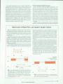
13 Comparing Manufacturing Methods
18
Authors
The Role of Doppler Ultrasound in Cardiac Diagnosis, by Raymond G. O'Connell, Jr.
Data shift blood flow anomalies can be obtained by observing the shift in frequency of
ultrasonic imaging pulse echoes.
Doppler Effect: History and Theory, by Paul A. Magnin The shift in the frequency of
sound for moving sources and/or listeners is described with its application for medical
analysis.
27 Johann Christian Doppler
O H Power and Intensity Measurements for Ultrasonic Doppler Imaging Systems, by
I James body Carefully controlling the acoustic energy transmitted into the human body
requires accurate analysis methods.
O £- Extraction of Blood Flow Information Using Doppler-Shifted Ultrasound, by Leslie I.
O O Halberg and Karl E. Thiele Frequency shifts in ultrasonic echoes are detected by means
of specially designed filters and a quadrature sampler.
37 Continuous-Wave Doppler Board
39 Observation of Blood Flow and Doppler Sample Volume
A -4 Modifying an Ultrasound Imaging Scanner for Doppler Measurements, by Sydney M.
I Karp Changes in timing, more precise focusing, processing enhancements, and powerlimiting software had to be developed.
A f- Digital Processing Chain for a Doppler Ultrasound Subsystem, by Barry F. Hunt,
rO Steven C. Leavitt, and David C. Hempstead Time-domain quadrature samples are con
verted into a gray-scale spectral frequency display using a fast Fourier transform, moment calcu
lations, and digital filtering.
Editor. Richard Supervisor, Dolan • Associate Editor, Business Manager, Kenneth A Shaw • Assistant Editor, Nancy R- Teater • Art Director, Photographer. Arvid A. Danielson • Support Supervisor, Susan E Wright
Illustrator, Nancy Contreras • Administrative Services, Typography, Anne S. LoPresti • European Production Supervisor, Michael Zandwijken
© Hewlett-Packard Company 1986 Printed in U.S.A.
2 HEWLETT-PACKARD JOURNAL JUNE 1986
© Copr. 1949-1998 Hewlett-Packard Co.
In this Issue
The integrated circuit artwork on our cover this month was drawn automat
ically the what's sometimes called a silicon compiler. As the authors of the
article on page 4 explain, "The process of silicon compilation is analogous
to the role of high-level language compilers in software engineering. The
designer specifies the behavior and/or structure of the desired circuit in a
high-level language. Working from the high-level specifications, the silicon
compiler generates the detailed circuitry programmatically. This not only is
faster than design by hand, but also allows system designers not familiar
with article design techniques to create an 1C chip." The subject of the article
is a high-level language used in-house by HP designers to specify a chip. Called ICPL, for
Integrated Circuit Procedural Language, it's a Lisp-based language similar to MIT's DPL.
About as new as silicon compilation is just-in-time manufacturing, the technique pioneered in
Japan and now spreading throughout the world. An estimated 250 plants in the U.S.A. have
implemented it and most large manufacturing companies are testing the concept. The article on
page 1 to just-in-time the design of HP JIT, an HP software product intended to be used by just-in-time
manufacturers for material requirements planning and production control. Worthy of note are the
methods used by the software designers to develop a package with no examples or standards
to use just-in-time guidance. Working with HP manufacturing divisions starting up just-in-time facilities,
the software designers tried out ideas using throwaway prototypes before finally writing specifica
tions and code.
The remaining six articles in this issue discuss a Doppler enhancement for HP's medical
ultrasound imaging system, first featured in these pages in October and December of 1983. In
ultrasound imaging, high-frequency sound waves are bounced off structures inside the body,
letting physicians see the body's inner workings without surgery or health risk to the patient. The
Doppler system augments the normal ultrasound image by adding information about the velocity
of blood flow and organ movements. On page 20, Ray O'Connell discusses the role of Doppler
ultrasound in cardiac diagnosis. On page 26, Paul Magnin presents Doppler history and theory
and tells us a little about Johann Doppler (page 27). The articles on pages 35, 41 , and 45 describe
the design of the HP Doppler system, which can be added easily to any HP ultrasound imaging
system. to page 31, James Chen tells how ultrasound power and intensity are measured to
ensure patient safety.
-R. P. Do/an
Editor
What's Ahead
Next computer issue will describe the design of HP's portable computer family — The Portable
and Portable Plus. Memory management, low-power operation, I/O and data communications,
liquid-crystal display control, and creation of custom plug-in ROMs are some of the topics. Also
featured will be an article about the latest capabilities of HP-UX, HP's version of the UNIXâ„¢
operating system, now available on HP 9000 Series 300 Computers. We'll also have the design
story of troubleshooting. HP 4971 S, a protocol analyzer for local area network installation and troubleshooting.
JUNE 1986 HEWLETT-PACKARD JOURNAL 3
© Copr. 1949-1998 Hewlett-Packard Co.
Integrated Circuit Procedural Language
ICPL is a Lisp-embedded procedural layout language for
VLSI design. Circuit design in ICPL involves writing and
working with programs that resemble procedures, take
parameters, and can use the full symbolic programming
power of Lisp. This allows circuit designers to write highlevel software that procedurally builds ICs.
by Jeffrey A. Lewis, Andrew A. Berlin, Allan J. Kuchinsky, and Paul K. Yip
IN RECENT YEARS, the design and fabrication of elec
tronic circuits on microchips has achieved the level of
very large-scale integration (VLSI). It isn't uncommon
today for a single chip to contain hundreds of thousands
of transistor devices, and we are beginning to see designs
where the component count exceeds one million devices.
With this dramatic increase in chip density comes an
equally pronounced increase in the complexity of the cir
cuit designs, resulting in a design bottleneck in the trans
formation of functional specifications into manufactured
products.
Conventional approaches to integrated circuit design
view circuits as a collection of rectangular regions — the
geometrical patterns used to define the devices on an 1C
chip. Circuit synthesis traditionally has been boiled down
to the art of handcrafting this large collection of rectangles,
most recently accomplished through the use of computerbased graphic editing. This manual approach is highly tedi
ous and error-prone when dealing with hundreds of
thousands of rectangles, where one misplaced or under
sized rectangle can cause catastrophic malfunction in the
circuit. In addition, the designer must constantly juggle
many conflicting criteria such as total chip area, power
consumption, and signal delay. As the number of compo
nents grows, these interrelationships become exponen
tially more complex. This complexity causes many design
ers to leverage their designs by using as many pieces of
old designs as possible. But since integrated circuit pro
cesses are changing so rapidly, very few old designs can
be used in new ones. The same type of adder, for example,
must be redesigned for every fabrication process it is used
in (see Fig. 1). Clearly, more automated mechanisms for
designing circuits are needed.
Silicon Compilation
Silicon compilation is a burgeoning subdiscipline of
computer-aided design (CAD) that addresses the problem
of managing VLSI complexity by automatically synthesiz
ing complex designs from high-level architectural descrip
tions. Variously referred to as systems for silicon assem
bly, module generation, macrocell assembly, or automated
layout, silicon compilation tools come in many variations.
What they have in common is that they raise the level of
abstraction at which the chip designer operates so that the
designer is more insulated from the complexity and vari
ation in lower levels. The designer is freed from performing
the tedious and error-prone tasks required by detailed man
ual layout of rectangles. Exploration of alternative architec
tures is simplified, making it easier to create more efficient
and cost-effective designs.
The process of silicon compilation is analogous to the
role of high-level language compilers in software engineer
ing. The designer specifies the behavior and/or structure
of the desired circuit in a high-level language. Working
from gen high-level specifications, the silicon compiler gen
erates the detailed circuitry programmatically. This is not
only faster than design by hand, but also allows system
designers not familiar with 1C design techniques to create
an 1C chip. Silicon compilation ultimately makes chip de
sign accessible to every circuit design engineer.
One popular mechanism by which silicon compilation
tools generate circuit artwork programmatically is known
as procedural layout. In the procedural layout paradigm,
a chip design resembles a software program. Circuit parts
resemble subroutines, take parameters, and can be "called"
by other parts. Thus, smaller parts can be hierarchically
built into larger parts, freeing the designer to concentrate
on higher-level issues. This provides a high degree of de
sign leverage. Parts generated programmatically are also
less prone to error than parts drawn by hand. One reason
is that values such as the size of a component or the spacing
between two components can be expressed as fabrication
process variables rather than by hardcoded numbers. De
signers can also specify a part's location relative to other
parts.
We chose the Lisp programming language as a basis for
silicon compilation and procedural layout design tools for
several reasons. After more than 30 years of language and
application development, the Lisp environment is unequaled in providing a powerful set of editing and debug
ging aids that translates into a friendly and extensible user
interface. Lisp is symbolic, meaning that it naturally cap
tures the way in which "real world" knowledge is rep
resented for problem solving. The interactive nature of Lisp
allows for a rich debugging environment for development
of both procedural layout design tools and the circuit de
signs that use them. Dynamic linking and loading provide
a high degree of incrementalism for exploratory program
ming, and Lisp can be compiled for production-quality
programs.
4 HEWLETT-PACKARD JOURNAL JUNE 1986
© Copr. 1949-1998 Hewlett-Packard Co.
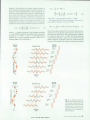
Implant
Diffusion (n and p)
Contact
Polysilicon
•
(a)
Fig. 1. /As a process technology
changes, the placement and size
of the rectangular elements form
ing a circuit element must be al
tered to achieve similar perfor
mance, (a) NMOS-C cell, (b) Equi
valent NMOS I/I cell, (c) Similar
CMOS-H cell. All cells were built
using the same ICPL code and dif
ferent fabrication process libraries.
(b)
Furthermore, the Lisp environment is the natural founda
tion for communication between CAD applications and
powerful Lisp-based expert systems tools. Any tool that is
embedded in Lisp can be invoked by any other to solve a
partial problem or can be used as the top-level design sys
tem. Thus, CAD functions can be used within rules and
knowledge-base queries can be called from within CAD
functions (see box on page 8). In addition to expert system
capability, other advanced programming techniques such
as object-oriented and data-driven programming are readily
accessible.
Finally, the Lisp environment provides extensibility of
both the tool set and the knowledge base to drive it. Extend
ing programs in conventional programming languages re
quires recompiling a fairly large world, or providing a pro
gram is covers all possibilities by run-time tests. This is
not necessary in Lisp, where functions are dynamically
recompilable and relinkable.
ICPL
HP's Integrated Circuit Procedural Language, or ICPL, is
a Lisp-based language that can be used by circuit designers
within HP to write programs that describe an integrated
circuit's layout. It is based on the Design Procedure Lan
guage (DPL) developed at MIT's Artificial Intelligence Lab
oratory1 and has been modified both in functionality and
structure to run on HP hardware and address the needs of
HP designers. Fundamentally, an ICPL designer writes a
program that describes how to build the layout and connec
tivity of a part rather than drawing it graphically. This
allows a user's cell definitions to be compiled, parsed by
the Lisp reader, and have embedded Lisp constructs like
any other Lisp dialect.
Simply being a language is not ICPL's strongest point.
Through the use of the symbolic programming capabilities
of ICPL, a designer can specify far more than a simple
geometric layout of a circuit. Cell libraries written in ICPL
have a significant advantage over traditional graphically
created libraries in that an ICPL cell can take parameters
like any other procedure to alter its functionality. For exam
ple, a buffer circuit can take as a parameter the capaciti ve
load it must be capable of driving and the speed at which
it must run, and then size itself to guarantee proper oper
ation for a particular application. Parameters can also be
used to create many variations on a particular design. For
example, a single register cell is capable of incrementally
adding the circuitry necessary to read to or write from
additional buses. A single cell with variable characteristics
eliminates the need for graphically generating the hundreds
of traditional cells that correspond to every possible com
bination of parameters.
The physical constraints imposed by a process technol
ogy are captured symbolically in ICPL via Lisp functions
that describe geometrical relations between parts. For
example:
(min-spacing 'poly 'diffusion)
will return a number that represents the minimum separa
tion between a rectangle on the polysilicon layer of an 1C
chip and a rectangle on the chip's diffusion layer. In tra
ditional design methodologies, a designer would have the
poly-diffusion separation rule memorized, and would
graphically separate the rectangles. In ICPL, a designer sim
ply includes a Lisp form that tells the system to separate
JUNE 1986 HEWLETT-PACKARD JOURNAL 5
© Copr. 1949-1998 Hewlett-Packard Co.
the two rectangles:
(align (» some-poly-rectangle)
(» center-left some-poly-rectangle)
(pt-to-right
(» center-right some-diffusion-rectangle)
(min-spacing 'poly 'diffusion)))
The Lisp form shown above would move some-polyrectangle such that its left center is to the right of some-diffusionrectangle by the minimum spacing between poly and diffusion.
ICPL captures the designer's reason for separating the two
rectangles, thus allowing the design to withstand minor
changes in the design rules of a process. If a cell is laid
out graphically and a process change occurs affecting the
minimum separation, the designer must graphically move
the rectangles to achieve the new minimum separation. In
most cases, there is not enough room to move a rectangle
to achieve a design rule change without hitting a new re
ctangle and consequently having to move it and its neigh
bors. These changes can propagate outward until every
thing in the cell must be moved. Because of their resistance
to change, graphic layouts tend to be discarded when an
1C fabrication process changes, thereby eliminating the
ability to reuse previous design work. Although it may take
a little longer to design a cell programmatically using ICPL,
such an effort is greatly rewarded by the ease with which
design changes can be achieved, and by the ability to use
a successful design for other projects.
ICPL incorporates a design management system to pro
vide an environment in which rectangles can be placed,
wires can be easily run, and a library of hierarchically
organized cells can be maintained. Connectivity informa
tion is maintained as it is declared by the designer, permit
ting integration of routing and automatic placement
utilities. Parameters are passed on a keyword-value basis,
defaulting to specified values if they are not supplied by
the caller. For example, consider the following ICPL de
scription of an NMOS inverter:
(deflayout INVERTER ((pullup-length *min-pullup-length*)
(pullup-width *min-gate-size*)
(pulldown-length *min-gate-size")
(pulldown-width *min-gate-size*))
(part 'pullup 'standard-pullup
(channel-length (» pullup-length))
(channel-width (» pullup-width)))
(part 'pulldown 'rectangular-fet
(channel-length (» pulldown-length))
(channel-width (» pulldown-width))
(top-center
(» bottom-center diffusion-connection pullup)))
It shows one other powerful feature of ICPL — other design
ers can look at the code and understand why things were
done in a certain way. For example, an explicit align state
ment will show that there is some sort of spatial relation
ship between two parts.
Another thing to notice about the above inverter example
is the procedural style of the deflayout. A deflayout is analo
gous to a Lisp defun or Pascal procedure definition because
it can take parameters and gives a sequence of steps to
perform. The inverter takes four parameters — pullup-length,
pullup-width, pulldown-length, and pulldown-width — which all have
default values taken directly from the fabrication process
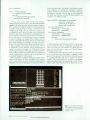
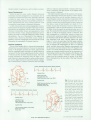
Fig. 2. ICPL display showing de
sign elements which can be ad
dressed and changed graphically
using a mouse.
6 HEWLETT-PACKARD JOURNAL JUNE 1986
© Copr. 1949-1998 Hewlett-Packard Co.
design rules. If a parameter is not passed to the inverter
code, then the default value will be used. Inside the deflayout
we have two part calls to deflayouts that have been previously
defined — standard-pullup and rectangular-fet. Since the four pa
rameters to the inverter code actually refer to the transistor
sizes of the constituent parts, we must pass these parame
ters down to the pullup and pulldown code actually re
sponsible for sizing the transistors. Finally, notice that the
last two lines of the deflayoirt align the part named pulldown
(of type rectangular-fet) so that the top center of the part aligns
with the bottom center of the diffusion connection of the
part pullup. We have specified the alignment of the pulldown
part such that no matter where the pullup part is placed
or how large it becomes, the pulldown part will always
align with it to form a correct inverter.
One long-term goal of our project is to foster the creation
of a large library of highly configurable ICPL cells which
will in effect be a collection of module generation proce
dures that work together. Several advanced users of ICPL
have written module generators for many of the regular
structures of VLSI design, including random access
memories, read-only memories, and programmable logic
arrays. In advanced ICPL code, even a simple cell such as
an inverter is created by a detailed procedure which creates
(continued on page 9)
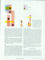
B-Bus
A-Bus
GND
REflD/WRITE fl - REflD/WRITE B - REFRESH
RERD/WRITE R - RERD 8 - REFRESH
REflD/WRITE fl - REFRESH
RERD fl - REflD/WRITE B - REFRESH
FEEDTHROUGH fl - REflD/WRITE B - REFRESH
REflD/WRITE 8 - REFRESH
REflD/WRITE H - REflD/WRITE B - NO REFRESH
REflD/WRITE R - RERD/WRITE B - REFRESH
TWICE POWER WIDTH
Fig. 3. with CMOS register cell. Some of the fifty possible configurations with two
buses are shown.
JUNE 1986 HEWLETT-PACKARD JOURNAL 7
© Copr. 1949-1998 Hewlett-Packard Co.
Knowledge-Assisted Design and the Area Estimation Assistant
VLSI complexity has Increased to the point that it is not unusual
to spend several engineer years doing a state-of-the-art 1C chip.
Software development has faced similar problems. The software
engineering problem was handled by raising the level of abstrac
tion at which the programmer operates. Aspects of the solution
are the use of higher-level languages for software developers
and new programming methodologies and tools to handle the
organizational complexity of large programming projects. VLSI
design complexity requires a similar solution. One preliminary
step Is the use of module generators, which allow the designer
to build large 1C parts such as random access memories without
needing to pay attention to the detailed artwork Implementation.
Knowledge-Assisted Design Framework
At HP's Cupertino Integrated Circuits Division, efforts are under
way towards the realization of a knowledge-assisted design
(KAD) system. We use the term knowledge-assisted to represent
the synergy of traditional CAD tools, algorithmic knowledge, and
artificial-Intelligence (Al) software technology. Primary motiva
tions for such a system Include:
• Supplementing, not replacing, the designer. Not all designers
who wish to take advantage of VLSI capabilities can do so
using traditional CAD tools and methodologies. This is be
cause of the vast amounts of knowledge needed to use these
tools to perform VLSI design. In addition to the VLSI-specific
knowledge, the amount of knowledge needed just to apply
the right tool to the right problem Is considerable. An environ
ment that eases the use of new tools for the designer would
be quite useful.
• Forming the communication medium in which all parties In
volved can share and retain Information and constraints. The
VLSI design process often requires coordination and com
munication among several different people. The system de
signer communicates specifications to the 1C designer, who
In turn communicates with other 1C designers, production en
gineers, and mask designers to achieve chip layout and pack
aging. Information lost in the transition between designers can
result in Increased design difficulties. Current design systems
are lacking In the ability to capture much of this information.
• Preventing the loss of expertise. A frequent occurrence Is the
departure or promotion of designers. The experience of those
designers Is normally lost or becomes very Inaccessible to
the designers that follow.
• Incorporating expertise from multiple experts. Designers often
have to consult with many other designers to achieve the best
possible results. However, the required expertise is frequently
not available when needed. As an alternative, the KAD system
could collect the knowledge of many expert sources, allowing
the designer to use the system as a readily accessible group
of consultants in the design and critique of the chip.
In one scenario, the designer presents to the system a block
diagram for a data path showing interconnections between regis
ters, missing and multipliers. Certain information may be missing
or incompletely specified. The system, in such cases, can assist
by filling in much of the omitted information. For example, the
chain length for an adder can be deduced from the number of
inputs and outputs. This, In turn, provides the means to estimate
the maximum time delay, the approximate area that the adder
will take up, and the power it will consume. The environment
should know what CAD tools are applicable for each design
problem, perform data translation, and interpret results of running
simulation and analysis tools.
We intend to provide a KAD framework for tool writers to build
knowledge-based tools upon and to provide an intelligent control
mechanism for incorporating those tools. We have chosen, as a
pilot project, a subpart In this scheme to use as a learning vehicle
for understanding what Is needed in the framework. Furthermore,
this build will bring out In more detail the issues Involved In build
ing expert systems within such a framework.
The pilot project is a knowledge-assisted tool for aiding the
planning phase of chip design. Such a tool tracks design deci
sions, attempts to fill in missing details, propagates hints and
constraints, and allows the user to explore functional and struc
tural chip design alternatives. In the decomposition phase of
chip design, the choice of different design alternatives results in
differing impacts upon block and chip area, power consumption,
timing delay, and testability. Our initial pilot project will provide
feedback on one of these figures of merit — block and chip area
estimation for the design.
Thus, there are two parts In this tool. A front-end planning
assistant facilitates exploring of design alternatives and a backend area estimation expert provides analysis Information for de
cision making.
Planning Assistant
The front-end segment deals with representation and manage
ment in functional and structural hierarchies. The problem in
volved here is to record, distinguish, relate, and apply knowledge
of blocks to each new task. During a session, the planning assis
tant accumulates design vocabularies in terms of block names,
part types, and part properties In an attempt to identify design
intent and apply its knowledge towards the goal. It allows a
designer to build design hierarchy in the designer's own style
and terms, using little or no detailed Information. When performing
a task, it tries to supply the missing detail from facts described
by the user, from related works done by some other designers,
and from knowledge It has based upon its understanding of
similar designs. When these mechanisms fail, the system
prompts the user for just enough Information to continue the task.
The system thus aids In filling in forgotten details and Identifying
inconsistencies and unnecessary duplication. This should en
courage the exploration of as many alternatives as possible to
find the best design decision.
The planning assistant can also record useful information such
as hints and constraints to be used In later development phases.
This creates an on-line notebook capability for the designer and
improves Information flow between design phases. For example,
during the planning stage the system designer may have made
a design decision based on the assumption that the RAM module
will have an aspect ratio of 1:1. This vital information is stored
with the RAM block as the only acceptable aspect ratio. When
the design is transferred to the 1C designer to implement the
physical layout, this constraint is also communicated to the 1C
designer. The planning assistant can carry large amounts of
such information, previously informally passed on only by rough
sketches and verbal communication.
Area Estimation Expert
The back-end area estimation expert provides feedback that
can be used recursively in design decision making. We chose
8 HEWLETT-PACKARD JOURNAL JUNE 1986
© Copr. 1949-1998 Hewlett-Packard Co.
area be over several other candidate applications be
cause it is a hard physical constraint for which people usually
rely on the most experienced designers to provide answers. We
also believe that area estimation should be incorporated into the
early design planning phases because, if not done right, it causes
expensive global changes in floor planning and is very time-con
suming to fix after detailed layout has been done.
Block area can be estimated using information from a few
different knowledge sources. First, there are hardcoded numbers
for information that has not yet been formalized into any other
categories. Next, there are block sizes derived from block boun
daries of actual cell libraries the system has access to. Third,
there are routines that describe area characteristics for highly
flexible parameterized cells such as module generators. These
functions take the same set of parameters, but instead of generat
ing the entire physical layout, they only return a value for the
estimated area and aspect ratio for the block. Fourth, there is
the option, if similar designs exist, of using those designs as a
basis between information, provided the relevant differences between
designs are accounted for. For example, one can estimate the
area for a given block by using area information that exists for
a similar block in a different process technology if the two
technologies can be mapped from one to another by a numerical
transform. Finally, when these mechanisms fail to return a result,
the system has two further options. If the block can be further
decomposed into simpler blocks, the system will do so and at
tempt to apply the area estimation mechanisms on the compo
nent blocks recursively. If the block cannot be further decom
posed (i.e., it is a leaf cell), then the system will either calculate
the area based upon gate count or prompt the user for a value.
the layout based upon specified parameters that account
for connectivity requirements, power bus sizing, output
load, and aspect ratio.
Several features have been added to ICPL to aid the cre
ation of just such a large procedural cell library. An inte
grated avoidance capability allows wires to be routed and
parts to be placed without regard to specific design rules.
Connectivity information is maintained in the same data
structures as the layout. This allows detection of such de
sign errors as shorting two global nets together, and neglect
ing to wire a particular cell. Integrated connectivity means
that parts have net attributes just like size and location
attributes, and it means that all of the parts tied to a net
can be easily found for capacitance extraction or design
verification.
A graphical editing capability is also tightly integrated
into the ICPL design environment. Developing designs can
be viewed on a color display, with mouse-actuated access
to the ICPL data structures. Using the mouse, designers
have the ability to trace electrical networks, move parts
around on an experimental basis, and obtain descriptions
of the design hierarchy (see Fig. 2). Layouts entered graphi
cally can also be converted to ICPL code. Although graphi
cal entry is a powerful tool for experimenting with circuit
layouts, it is not recommended for the final library cell
because it does not capture the intent of the designer. Some
users find it helpful to begin a layout graphically and then
modify the ICPL code to include the placement constraints
that represent their intent.
Geometric structures and their combinations are rep
resented in ICPL as Lisp objects. Arbitrary properties can
To acquire the knowledge for this system, we have incorpo
rated in the project team the skills of an 1C design expert with
whom we have conducted a long series of interviews. Eventually,
we hope the system will capture his expertise in making use of
all the above information sources, partitioning problems, combin
ing cells, adjusting aspect ratios, consulting different but related
designs, making trade-offs, and setting up tolerance ranges for
block headroom based upon his confidence level at different
steps. There are also interesting techniques discovered in those
interview sessions that will contribute to the front-end planning
assistant as well, particularly in the way this designer makes use
of uncertainties at each phase and handles the iterative design
flow of making block definition, decomposition, and recomposition.
Area estimation is more than just adding up numbers. There
are assumptions upon which the estimation is made. Availability
of library cells and module generators, orientation, aspect ratio,
and relative placement of blocks, and intended signal paths are
just a few examples of these assumptions. These planning deci
sions dictate restrictions the subsequent chip recomposition
must follow and provide useful technical hints and tricks to help
develop layout details.
Benjamin Y.M. Pan
Michael How
Development Engineers
Allan J. Kuchinsky
Project Manager
Cupertino Integrated Circuits Division
be associated with a part, thus enabling Lisp programs such
as circuit extractors and cell compilers to store their data
on the parts themselves. Through properties, users can ex
tend ICPL to support virtually any configuration they
choose. For example, resistance and capacitance values
can be determined and tacked onto parts for use with a
user-developed circuit simulator. Furthermore, all ICPL
data structures are based in Lisp, thus enabling the ICPL
programmer to use the full power of the Lisp programming
environment.
ICPL is tightly integrated with HP's internal design sys
tems, permitting efficient interchange between ICPL and
various circuit simulators, graphical editors, and design
rule checking programs. Designers who use ICPL properly
can be assured that their designs will weather many process
and methodology changes before they become obsolete.
Applications of ICPL
Several complex module generators have been developed
using ICPL. A module generator automatically creates the
layout for a large piece of a chip, such as the RAM or ROM
section. Simpler library cells have also been designed that
allow a large combination of parameters to have a large
effect on the configuration of the cell. Only one generic
cell needs to be designed and stored in the cell library as
a template from which many different configurable cells
can be produced.
This feature can be shown in the example of the configur
able register cell (Fig. 3). This register cell can read from,
write to, not connect to, or both read from and write to
either of two buses. There is an optional refresh capability,
JUNE 1986 HEWLETT-PACKARD JOURNAL 9
© Copr. 1949-1998 Hewlett-Packard Co.
and the width of the power buses can be adjusted for different
current densities and spacing constraints. Fifty different
configurations of the register can be generated by passing
in different sets of parameters in the part call to the register.
This register cell shows that parameterization in ICPL al
lows a cell library to be more space efficient and provides
designers with greater flexibility in selecting the precise
cell configurations they want.
An example of a much larger ICPL module generator is
the Ramgen project at HP's Cupertino Integrated Circuits
Division. Ramgen is a program that captures, optimizes,
and generates a general-purpose static RAM (see cover).
The modules generated are designed to be equivalent to
off-the-shelf RAMs that can be easily inserted into a stan
dard-cell or custom chip. Organization and size of the RAM
are user-programmable by specifying the total RAM size
desired, the word size, and the aspect ratio. This will create
a RAM that will fit not only a variety of functional require
ments but also a variety of physical ones. These features
allow a chip designer to design a RAM at a high level with
the fast design-and-verify turnaround time of approxi
mately ten CPU minutes on an HP 9000 Model 236 Com
puter (instead of five months handcrafting time) for a 256bit to 16K-bit RAM. Beyond the time improvement, the
user is also guaranteed a working RAM. Ramgen has been
used for over a year in the design of nine chips.
One of the most comprehensive module generators under
development at HP is the Datapath generator. Datapath
enables a complete data path system to be generated from
a functional description. Input to the Datapath module
generator is a MADL (Multilevel Architecture Description
Language)3 behavioral description of the circuit and the
output is the geometric layout of the design in ICPL.
Datapath users are provided with two libraries: the MADL
library, which contains the behavioral descriptions for
simulation, and the ICPL library for artwork generation. A
designer only needs to specify the behavioral description
for the design and the order in which the library cells
should be placed to generate the full data path. The physical
layout of each cell is such that cells only need to be placed
adjacent to one another for all bus connections to be made
automatically. The cells can also be sized for different out
put drive capabilities by passing in the value of the capacitive load on the driven net. Since ICPL represents net-based
connectivity, the calculation of total capacitance of the net
is easily done by traversing the net and summing the capaci
tance of each cell. The design generated by Datapath is
readily testable since all the library cells have scan path
capability, allowing all the nodes in the design to be excited
and observed easily.
Advanced Work
ICPL has been extended in many ways to take advantage
of the powerful environment available in the HP 9000
Series 300 Computer family. Extensive use has been made
of the windowing system and the Starbase Graphics Li
brary, and ICPL has been rewritten in Common Lisp to
conform to that emerging standard. In addition, expert sys
tem tools for layout assistance and silicon compilation are
being integrated with the ICPL data structures (see box on
page 8). Although still in their infancy, expert systems for
CAD have begun to show their worth in solving problems
that were intractable using conventional programming
styles.
ICPL will provide the basis for powerful silicon compi
lation tools in the future. The productive Lisp environment,
the symbolic nature of ICPL, and integration with expert
systems will allow designers to design chips much more
rapidly than ever before. It is conceivable that an ICPLbased silicon compiler could take an initial chip specifica
tion, generate artwork, and continually iterate through the
design, refining the weakest areas (in size, speed, power
consumption, etc.) until the design converges on the op
timum. Users will be able to get the power of VLSI design
without needing to be familiar with the fine details of 1C
design techniques.
Acknowledgments
The authors would like to thank and acknowledge a
number of people for their contributions to ICPL. These
include William Barrett, Bob Rogers, and Mike Sorens for
their early work in the design and implementation of ICPL,
Bill McCalla, Joe Beyers, Marco Negrete, and the late Merrill
Brooksby for their support, Ira Goldstein, Martin Griss,
Craig Zarmer, Chris Perdue, Alan Snyder, and Gwyn Osnos
for their help with the Prism system (and with our early
questions), and certainly Liz Myers, Dave Wells, Jon
Gibson, Ed Weber, Pete Fricke, Shaw Yang, Duksoon Kay,
and Rick Brown, who have beautifully demonstrated the
feasibility of using Lisp-based design tools in building pro
duction chips.
References
1. J. Batali and A. Hartheimer, "The Design Procedure Language
Manual," AI Memo #598, VLSI Memo 80-31, Massachusetts Insti
tute of Technology, Artificial Intelligence Laboratory, September
1980.
2. B. Infante, M. Bales, and E. Lock, "MADL: A Language for
Describing Mixed Behavior and Structure," Proceedings of the
1FIP Sixth International Symposium on Computer Hardware De
scription Languages and their Applications, May 1983.
10 HEWLETT-PACKARD JOURNAL JUNE 1986
© Copr. 1949-1998 Hewlett-Packard Co.
New Methods for Software Development
System for Just-in-Time Manufacturing
New approaches in prototyping, next-bench involvement,
performance modeling, and project management created
a high-quality software product in the absence of standards
or existing systems.
by Raj K. Bhargava, Teri L. Lombard!, Alvina Y. Nishimoto, and Robert A. Passell
HP JIT IS A SOFTWARE SYSTEM that assists in the
planning and control of material and production
for manufacturing facilities operating with a new
manufacturing technique developed in Japan and known
as just-in-time. Just-in-time manufacturing reduces com
plexity on the factory floor by using fixed production rout
ings and a pull system for material handling. In a pull sys
tem, raw materials are delivered to the factory floor as they
are consumed in production. This simplifies manufactur
ing management.
About HP JIT
HP JIT is designed to be a stand-alone product or to run
in a combined environment with HP Materials Manage
ment/3000.1 The combined system allows a user to avoid
redundant parts and stock area data when both the tradi
tional work-order material requirements planning and justin-time philosophies are used in the same facility.
The majority of the HP JIT software runs on the HP 3000
Computer, using Hewlett-Packard's Application Customizer2
and Monitor3 technology. The Application Customizer and
Application Monitor are themselves software tools that are
used by application designers to engineer generalized soft
ware systems, and then by users to adapt the systems to
their individual needs. HP JIT also uses the HP 150 Personal
Computer as a management workstation. The HP 150 Com
puter can serve as the interface to the HP 3000 Computer
for accessing the material and production functions, or as
a stand-alone personal computer for access to local decision
support tools.
HP JIT is meant to complement the characteristics of a
just-in-time method of production, including:
• Fixed production routings on the factory floor
• Single-level bills of material (flat structure)
• Planning by production rate to accommodate steady pro
duction targets over a period of time
• Short production cycles featuring quick assembly.
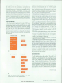
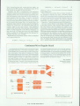
HP JIT has seven major software modules (see Fig. 1),
each of which addresses a different requirement of the justin-time manufacturing method:
• Parts and Bills of Material
• Rate-Based Master Production Scheduling
• JIT Material Requirements Planning
• Production Reporting and Post-Deduct
• Stock Areas and Deduct Lists
• Inventory Management
• Material Cost Reporting.
Parts and BiJIs of Material maintains basic information
on every part used in production, recording product struc
ture, standard costs, and data on product options and en
gineering changes. Its features include single-level manu
facturing bills of material, effectivity dates for engineering
changes, pseudoparent parts to represent subassemblies
consumed in production, multiple product options, and
ABC part classification.
Rate-Based Master Production Scheduling matches
proposed production and shipment schedules against back
log and forecast orders to manage finished goods inventory
more effectively. Planning is accomplished without work
orders, with monthly production of each end product based
upon a planned rate of output for that product per day.
Schedules for different production lines producing the
same product can be adjusted separately. The features of
this module include a predefined VisiCalc® spreadsheet,
"what-if" capability for production planning, graphics for
reporting of monthly plans, automatic data transfer be
tween the HP 150 Personal Computer and the HP 3000
Computer, an interface for forecast and backlog informa
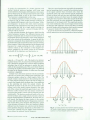
tion, and a five-year planning horizon. Fig. 2 shows a master
production schedule produced using HP JIT.
/IT Materia] Requirements Planning determines the
Personal Computer
Rate-B
Master
Production
Scheduling
Production
Reporting and
Post-Deduct
Selective
JIT MRP
Inventory
Management
Material
Cost
Reporting
^ ^ ^ M
Parts and
Bills of
Material
Fig. 1 . Seven major software modules make up the HP JIT
package for just-in-time manufacturing.
JUNE 1986 HEWLETT-PACKARD JOURNAL 1 1
© Copr. 1949-1998 Hewlett-Packard Co.
quantities of parts required to support the master produc
tion schedule, daily production schedule, and planned
extra use of component parts. JIT MRP reports can be run
selectively over a range of part numbers, controllers,
buyers, or dates, or according to selection criteria of the
user's choice in either daily, weekly, or monthly incre
ments, or some combination of these. The features of this
module include selective MRP by date range, component
part range, controller/buyer range, or other user-defined
attribute, single-level explosion, option mix planning, op
tion effectivity dates, and action/preshortage reports. Fig.
3 on page 14 shows a JIT MRP screen for entering select
criteria for an MRP run.
Manufacturing Control
Manufacturing control is carried out on the factory floor
• via the post-deduct transaction and the Production Report
ing and Post-Deduct module, which records actual produc
tion completed and, at the same time, relieves stock areas
of inventory consumed in assembly. Post-deduct is a onestep approach, as opposed to the traditional "issue and
receive" of a work-order-driven production reporting sys
tem. Defining a deduct point in HP JIT provides visibility
of the consumption and movement of materials on the fac
tory floor. As a part is built and passes through a defined
deduct point, HP JIT records the creation of the part, incre
menting its inventory quantity and decrementing the in
ventory quantities for its components. On-line review of
actual versus planned production is provided in HP JIT.
The features of the Production Reporting and Post-Deduct
module include post-deduct of up to 25 options per parent
at a time, post-deduct by engineering change level, post-de
duct at subassembly or end-product levels, summarization
capability that allows tuning of the HP JIT system by the
user to optimize performance, and actual production re
porting by the hour or by the day. Reviews of planned
versus actual production use graphics. Fig. 4 on page 15
illustrates an HP JIT post-deduct transaction.
The Stock Areas and Deduct Lists module further defines
the manufacturing process. Corresponding to each deduct
point is a deduct list which associates the component parts
and their quantities consumed at that deduct point with
the stock areas from which those components were picked
in the assembly process. The features of this module in
clude multiple stock areas per part, multiple deduct-point
types (intermediate, end-of-line, subcontract), multiple de
duct points per line, multiple production lines per product,
and split, merged, and mixed-mode production lines.
inventory Management maintains the current status of
each stock area and updates its status through the post-de
duct, scrap, or extra use transactions. The features of this
module include on-line inventory balances, multiple stock
area status codes (available, unavailable, scrap, inspection),
recording of scrap and extra use, two-stage cycle counting,
and inventory count and adjust capabilities.
Material Cost Reporting summarizes accounting infor
mation on materials produced during an accounting period.
This module features production data summarized by indi
vidual product, exception data recorded on an individual
transaction basis for visibility, and material variances cal
culated based on scrap and extra use recorded.
Development Cycle
The HP JIT development project was significantly differ
ent from software deveploment projects that preceded it.
New methods for engineering this type of software were
introduced to meet the objective of producing a high-qual
ity product in a shorter period of time than had been typical.
Fig. 5 on page 16 shows two time lines contrasting the
traditional and HP JIT development cycles. The remaining
sections of this article detail some of the methods used in
the HP JIT project to change the typical project cycle.
Prototypes
The HP JIT project provided an opportunity to try a dif
ferent approach in the investigation and external specifica
tion phases of a large software project.
The traditional method produced investigation and ex
ternal specification documents for review, but these docu
ments were generally felt to be an ineffective method of
Hewlett Packard - ***YOUR COMPANY NAME *
Master Production Schedule
P r o d u c t
N u m b e r
9 3 8 2 7 A
12/85
21
01/86
23
02/86
19
03/86
23
10
0
15
0
10
0
10
80
80
Backlog Orders. . . .
Order Forecast. . . .
Carry Forward Orders.
TOTAL Orders
200
50
0
250
180
50
0
230
130
90
0
220
100
130
0
230
Production/month. . .
Beginning FGI ....
TOTAL Shippable Units
325
0
325
230
75
305
190
75
265
1840
45
1885
M o n t h
Number of working days.
Past Due Production
Production Rate/Day (prev plan)
(curr plan)
12 HEWLETT-PACKARD JOURNAL JUNE 1986
© Copr. 1949-1998 Hewlett-Packard Co.
Fig. 2. An HP JIT master produc
tion schedule.
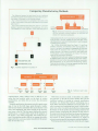
Comparing Manufacturing Methods
The difference between the batch stock flow of a traditional
manufacturing system and the demand-pull stock flow of a just-intime system is illustrated by the following example.
Fig. 1 shows that product A is composed of two parts, B and
C. Part C is purchased, while part B is fabricated from purchased
parts X and Y.
Fig. 2 shows traditional batch stock flow. Parts X, Y, and C are
received, inspected, and placed in the warehouse. An X and a
Y are released to a work order W01, which uses these parts to
Raw Purchased Material
X, Y. C
Receive
Finished
Goods
Inventory
Inspection
Fig. 3. Demand-pull stock flow. Just-in-time manufacturing
may also eliminate incoming inspection so that parÃ-s flow
directly from receiving to production.
create subassembly B, which is returned to inventory. Subassembly B and part C are then released to work order WO2, which
uses these parts to create the finished product A, which is placed
in finished goods inventory.
Fig. 3 shows demand-pull stock flow. Parts X, Y, and C are
received, inspected, and delivered to their stock locations. An
X and a Y are used in the creation of subassembly B, which then
travels down the production line to the point where part C is
added, resulting in the creation of product A. Raw material and
finished goods inventory adjustments are made at this time by
means of the post-deduct transaction.
Besides eliminating the work orders and subassembly storage
of traditional batch stock flow, demand-pull stock flow makes it
possible to introduce further improvements that are now consid
ered characteristic of the just-in-time manufacturing method.
These are the elimination of incoming inspection and the flow of
parts directly from receiving to production.
Fabricated Parts (A.B)
Purchased Parts (X.Y.C)
Fig. 1. Assembly sequence for a product A.
Warehouse
Raw Material
Subassembly
Assembly 1
B
Finished
Goods
Inventory
B
C
X, Y, C ,
Receive
PO
Receive
INSP
Issue
WO1
Receive Issue
W 0 1 W 0 2
communication. Many readers found it difficult to vis
ualize the final product solely on the basis of written
specifications, and often did not review the documents
carefully.
External specification documents typically spend a great
deal of time in the draft stage, going through a lengthy
draft-review-rewrite cycle before they can be shown to end
users, field marketing, and others outside of the develop
ment team in the lab. The time spent drafting the external
specifications is a period when much of the progress on
the project is not readily measurable. This makes the pro
cess of creating the product difficult to manage during this
stage, and in the worst case, makes it possible for the project
team to lose their focus.
Receive
WO2
Fig. 2. Traditional batch stock
flow.
With these concerns in mind, we decided to try a differ
ent approach on the HP JIT project. Rather than use the
traditional method of creating an external specification
document, we decided that software prototyping was a
much better channel for feedback and would allow us to
solicit customer and marketing input early in the develop
ment cycle, when it would be most effective in determining
the feature set of the product and providing a basis for the
internal design. Prototyping the software at this point in
the project provides the best basis for asking vital questions
about the proposed feature set of the product, and for seek
ing answers to these questions iteratively, by means of
successive prototypes that incorporate customer feedback.
Prototyping also helped reduce the risk in the early stages
JUNE 1986 HEWLETT-PACKARD JOURNAL 13
© Copr. 1949-1998 Hewlett-Packard Co.
of product engineering by unifying the development team's
own understanding of the product, making the features and
functionality of the system more tangible. This helped iden
tify potential problems in system design early and mini
mized costly engineering redesign in the later phases of
the project.
Our strategy for implementing prototypes was to produce
a prototype in three to four weeks. We felt prototypes
should be done quickly, using whatever tools were avail
able. Their purpose was to allow us to iterate the solutions
to vital questions.
The prototypes were not meant to be an early stage of
the coding phase, since the prototypes were to be thrown
away after the features or problems they .addressed were
understood. No attempt was ever made to use any actual
prototype implementation later, since we felt that this
would inhibit the project team from solving the problems
quickly. If an actual prototype were to be used later as the
basis for some effort in the coding stage of the project, we
felt that we would quickly become overly concerned with
engineering the "perfect" prototype during the investiga
tion and lose our focus on asking vital questions and solving
problems that the prototypes were supposed to address.
In the JIT project, there were six simulators and pro
totypes as follows:
• Screen simulator I (3 weeks). Test high-level product
definition.
• HP 150 prototype of HP 3000 link (4 weeks). Test tech
nology of HP 150 link.
• HP JIT functional prototype (3 weeks). Test design of
data base and critical transactions (performance).
E Screen simulator II (3 weeks). Test functional design.
• Screen simulator III (3 weeks). Test user interface.
Screen simulator IV (3 weeks). Refinement.
At the end of this process a concise document was written
to confirm the consensus of the customer, marketing, and
lab input we had received on the prototype models of the
HP JIT
product. Instead of the traditional approach, where a docu
ment is produced for review and revision before the prod
uct feature set is determined, the document produced for
our project was effectively a summary of what the project
team had agreed upon, based on the results of an iterative
prototyping process.
To summarize, in the traditional method, documents
were an ineffective method of communication. People often
did not review documents carefully. It is difficult to vis
ualize a software system solely through the use of a docu
ment. There could be long periods of time during the draft
ing of the document when no progress on the project was
visible. A lengthy review was required to get agreement on
product specifications, and there was little involvement
outside of the development lab before the document review
cycle was completed. This brought considerable risk to the
process of developing the product and made it difficult to
measure whether the project was on track or not.
In contrast, the HP JIT project used prototypes to provide
a tangible display of product functions and features during
the design phase of the project. This proved to be an ex
tremely effective method for communication and elicited
more thorough feedback from potential users, who could
visualize the final product more fully based on the initial
prototypes. The many iterations of the product prototypes,
each one progressively refining the feature set of the prod
uct, provided the product with an opportunity to establish
many short milestones and made progress during the de
velopment phase more visible and measurable. The in
volvement of end users and marketing during the early
phase of product design decreased the risk of redesign and
reengineering later on in the project.
Next-Bench Involvement
HP is widely recognized as an industry leader in imple
menting the just-in-time production method. A primary
objective of the HP JIT project was to work closely with
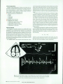
Select Criteria for MRP Run
Ending date for MRP
daily report (mmddyy)
SELECT MRP
Run MRP
now? (Y/N)
Component Part Selection Range
F r o m : Ã Â ¡ . :
T o : |
Controller ID Selection Range
F r o m :
 ¡ I I
T o :
Other Criteria Selection Range
From: ¡
COMMAND:
Planning
Pe rf o na
14 HEWLETT-PACKARD JOURNAL JUNE 1986
© Copr. 1949-1998 Hewlett-Packard Co.
Fig. 3. An HP JIT screen for enter
ing select criteria for an MRP (ma
terial requirements planning) run.
HP divisions that practice JIT so that we could quickly
develop a product that would suit HP's internal needs as
well as those of the marketplace.
To meet both internal and external needs, several impor
tant requirements must be satisifed. There must be both
management commitment and individual commitment
throughout the project teams at divisional sites participat
ing in the development process. More than one external
division must be involved, and each must dedicate some
one full-time to the project. In practice, the partner division
teams communicated among themselves so effectively that
many disagreements about product requirements were re
solved without intervention by the development team in
the software lab.
The partner divisions played an important role in all
phases of the project. During the design phase, increased
productivity in the software development lab resulted from
their review of the prototypes and specifications, eliminat
ing a significant amount of guesswork on the part of the
design engineers when adding new product features. The
partner divisions helped eliminate guesswork during the
final coding phase by testing product quality and verifying
that the software indeed solved the problems it was de
signed to handle and correctly provided the features
specified. The credibility of HP JIT as a product was in
creased by the combination of HP's being looked upon as
a just-in-time manufacturing leader in the U.S.A. and the
partner divisions' acting as reference sites showcasing HP
JIT.
Application Architecture
HP JIT was designed to be coded in Pascal and to use
the CT (customizable technology) software tools developed
by HP's Administrative Productivity Operation.4 CT soft
ware tools free the application designers from much of the
detail work involved in opening data bases and files, han
dling terminals, and updating screens. HP JIT went farther,
HP JIT
however, and placed many of the common calls to th'
underlying CT tools inside of utility subroutines in the
product that could be called from any of its modules (see
Fig. 6). Utilities were written for data base searches, screen
handling, and transaction logging, as well as other more
specific JIT functions. The initial impetus behind the de
velopment of these utilities was to avoid duplication of
Pascal source code, but each utility was designed for
maximum flexibilty so as to be usable by transactions and
modules yet to be developed. Through the use of flexible
common utilities, duplication of Pascal source code
throughout the HP JIT software was nearly eliminated.
Building an application such as HP JIT on top of a layer
of utility procedures has many significant advantages.
Eliminating code duplication not only reduces overall code
length, but also reduces source code clutter in individual
modules, thereby helping to preserve transaction clarity.
Relying on many shared utility procedures eliminates the
risk of errors caused by oversight and accident when rep
licating source code throughout many individual modules.
Code maintenance and product enhancement are made
simpler, since a correction or enhancement can often be
made in a utility module and effected immediately through
out the entire application by replacement of the utility
module alone. Some utilities (e.g., screen handling and
data base operations) can be used by similiar software sys
tems, saving time and effort when developing and testing
other products. Reliability is increased, since a utility
called by several different individual transactions is excercised thoroughly during testing.
Some typical HP JIT utilities are:
compare_lines On a screen with multiple data entry
lines , determine that the user hasn't
entered any duplicates.
dataset_msg Inform the user about the success or
failure of finding or not finding a
requested data item.
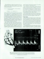
POST DEDUCT
Post Deduct a Parent Part
Parent Part Number Option ID
Deduct
Point ID
Quantity
Deducted UM
EC
Level
EC Level
Used
Description
Change Default
EC Level?
EU
ÃY/N)
COMMAND:
Perforn
Deduct
Pull
Part
Receive Scrap |M Hfg Cntl
Part Corapnent Compnent Menu
Fig. 4. The HP JIT post-deduct
transaction records production
completed and simultaneously re
lieves stock areas of inventory
consumed in assembly.
JUNE 1986 HEWLETT-PACKARD JOURNAL 15
© Copr. 1949-1998 Hewlett-Packard Co.
find datasetrec,
multi_find_dataset
process maint
valid_in_security
valid input
open_message_file
lock datasets
input_required
Locate an entry or entries that match
a set of criteria parameters in the
specified database.
Do all screen handling for the HP JIT
maintainance transactions.
Check user access to screen.
Determine that key input fields on
screen are valid for the transaction.
Open a specified MPE message file.
Create it if it doesn't exist.
Lock the specified data items or sets as
specified by key parameters.
Verify that a list of fields has been
input.
where D is the total number of deduct points, P is the total
number of parents, L is the number of production lines,
and E is the total number of deduct list elements.
This model showed that for a low-volume customer, even
the best case would cause this transaction to take 2.7 hours
to process one hour of customer data. This meant that even
for a low-volume customer, the post-deduct transaction
would never catch up with incoming data that it was in
tended to process.
To solve this problem, we designed this transaction to
summarize the processing of the data, allowing the cus
tomer to specify the summarization interval. The model
allowed us to provide a formula to help customers decide
what summarization interval would fit their type of data
and rate of production. The formula is:
Performance Modeling
In the HP JIT project, we decided to try a new approach
to the performance testing of our application projects. The
old method collected a lot of data with little idea of the
questions being answered. In addition, performance tests
tended to be done after the product was coded. Any bad
news was received too late, when it was costly to redesign
and recode.
The HP JIT project established performance objectives
in customer terms before any coding or design had been
done. After we first modeled performance, we continued
to refine the model based on actual performance test results.
Our performance model uncovered a major performance
problem with our most critical transaction, post-deduct,
before we completed designing or began coding the prod
uct. One post-deduct transaction can result in up to 400
separate data base updates. According to the model, the
maximum production rate, or the rate that HP JIT can han
dle with real-time updates of component part consumption,
is given by:
Maximum
3600-0. 75P
Production =
0.25 + 1.5D/L + E/L
Rate
Summarization
Interval
1.25DP/L + 0.75P + E + 900R
1-0.5DR/L
where D, P, L, and E are as above and R is the total produc
tion rate per second.
Quality Procedures
Quality was built into HP JIT using a variety of tech
niques. In the lab, formal design reviews and code inspec
tions were used throughout the development process, and
this contributed to improving the overall functionality and
correctness of the code for each module. The use of utility
routines to perform shared functions for separate applica
tion modules contributed to quality by eliminating manual
duplication of code. Since these utilities are accessed by
a variety of calling routines, any defects or deficiencies
were detected early, and the utilities eventually proved to
be very robust. HP JIT also made use of its partner divisions
within HP as alpha and beta test sites during the design
and development phase of the product. These partners were
actively implementing just-in-time manufacturing tech-
18 Months to 2 Years
Lab
ES ID
Code
Test
(a)
E S
I D
C o d e
T e s t
M R
A=Document
• =Code
I = Investigation
ES = External Specif ¡cation
ID =lnitial Design
PM = Performance Model
PT = Performance Test
Alpha = Alpha Test (Lab Test of
Functionality)
Beta = Beta Test (Marketing Test
of Document and Support)
(b)
16 HEWLETT-PACKARD JOURNAL JUNE 1986
© Copr. 1949-1998 Hewlett-Packard Co.
Fig. 5. (a) Traditional software de
velopment cycle, (b) The HP JIT
development cycle was shorter
than the traditional cycle. Software
prototyping replaced the usual in
vestigation and external specifica
tion phases.
ñiques and thus were qualified to assist in the design of
the product and test its functionality. Each partner was
allowed to narrow its focus to a particular testing objective.
This made the process of testing more manageable and the
testing more thorough. "Mini-releases" of HP JIT to the
partner divisions throughout the design and development
stages kept the testing effort progressing actively and kept
the partners from feeling overwhelmed by bulky new ver
sions of the product with large doses of new functionality.
Each of the partner divisions was assigned a member of
the HP JIT lab team for support, providing quick feedback
and fostering closer ties throughout the entire development
team.
Project Management
One of the essential ingredients that made HP JIT a suc
cess was the innovative project management. We recog
nized the need to make quick decisions as a team. At times,
this meant taking action even when we did not possess
complete or adequate information. However, we were will
ing to take risks and accept the fact that we would learn
along the way. We expected that as we gained more experi
ence our decisions would have to change. We did not resist
change, but managed it so we could meet our milestones
and objectives.
Transaction Code
Utility Code
Security Check
Screen Handling
Data Base
Utilities
Error Messages
Transaction
Utilities
Locking
(a)
Transaction Code
Utility Code
Security Check
Screen Handling
Utilities
Error Messages
We planned milestones in 4-to-6-week intervals. These
milestones were measureable and very visible to people
involved in the project. The lab team then viewed these as
"hard" milestones and every effort was made to meet them.
With these frequent milestones it became much easier to
measure our progress, providing focus and great satisfac
tion to the team as we met each milestone.
We emphasized leveraging existing resources and avoid
ed duplication of effort. At each step we tried to direct our
efforts to activities that could be used in the final product
package. For example, the external specifications became
the starting point for the user manual. We always went
through iterations before making decisions and starting to
build. However, once a component of the product had been
built or a specification defined, we resisted augmentation
and rework. Early in the project all dependencies were
defined and contingency plans were developed. We recog
nized that some dependencies were absolutely essential
and no backup was available. However, we made it an
objective to minimize dependencies on the critical path.
The three most important overall goals for the HP JIT
project were:
• To invent a high-quality software product where there
was none before, either internally or externally
• To meet all scheduled milestones, the most important
being the MR (manufacturing release) date, which was
stated at the beginning of the project
• To increase the productivity of engineers in designing
this type of software product.
The design of the product was influenced from its earliest
stages by groups that would have a major influence on its
ultimate success: JIT practioners and HP product market
ing. The process of designing functionality and quality into
the product was enhanced by the use of rapidly developed
prototypes as a basis for communication about product
function and design. The establishment of frequent mile
stones, each with a deliverable part of the product (from
prototype to completed module) aided in sustaining the
momentum of the project team and kept the effort success
fully on track from start to finish.
Acknowledgments
Nancy Federman was the R&D project manager for HP
JIT until the first release of the product. We would like to
thank her for her leadership and for developing some of
the figures used in this article. We would also like to thank
product team members Steve Baker, Marc Barman, Jim
Heeger, Pamela Hinz, Kristine Johnson, Mike Kosolcharoen, Mary Ann Poulos, and Chris Witzel for their contribu
tions in developing HP JIT. Our thanks also to Computer
Systems Division (Cupertino and Roseville), Disc Memory
Division (Boise), San Diego Division (San Diego), and Van
couver Division (Vancouver) for their active participation
and feedback.
(continued on next page)
Data Base
Utilities
(b)
Fig. 6. (a) Traditional software coding, (b) HP JIT coding
built the product on a layer of utility procedures.
JUNE 1986 HEWLETT-PACKARD JOURNAL 17
© Copr. 1949-1998 Hewlett-Packard Co.
References
1. N. C. Federman and R. M. Steiner, "An Interactive Material
Planning and Control System for Manufacturing Companies,"
Hewlett-Packard Journal, Vol. 32, no. 4, April 1981.
2. L. E. Winston, "A Novel Approach to Computer Application
System Design and Implementation," ibid.
Authors
June 1986
4 — ICPL ;
Allan J. Kuchinsky
^^^^^^^^^J With HP since 1978, Allan
Kuchinsky manages the
Lisp tools group at HP's
Cupertino 1C Division. His
contributions include work
on HP Production Manage
ment/3000 and on ICPL. He
is a coauthor of three tech
nical papers and is a
member ofthe IEEE and the
American Association for Artificial Intelligence.
Allan was born in Brooklyn, New York and studied
psychology at Brooklyn College (BA 1971). He
taught science at a New York City secondary
school and was a high school biology teacher ¡n
Mexico City. He has also worked as a musician. Be
fore coming to HP he completed work for an MS
degree ¡n computer science ¡n 1 978 at the Univer
sity of Arizona. Now a resident of San Francisco,
he's married and has one son. He enjoys playing
his guitar, listening to reggae music, and spending
time at music and comedy clubs. He's also fond
of reading science fiction and murder mysteries.
3. B. D. Kurtz, "Automating Application System Operation and
Control," ibid.
4. J. L. Malin and I. Bunton, "HP Maintenance Management: A
New Approach to Software Customer Solutions," Hewlett-Packard
Journal, Vol. 36, no. 3, March 1985.
Andrew A. Berlin
Robert A. Passed
| With HP since 1985, Andy
Berlin is an R&D engineer
at HP's Cupertino 1C Divi
sion. He has contributed to
the development of ICPL
and has taught an HP soft• ware engineering class. He
^Tfc^^ I was born ¡n New York City
and holds a 1 985 SBEE de
gree from the Massachu
setts Institute of Technology. Andy lives in Cuper
tino, California, and enjoys playing piano.
Born in Milwaukee, Wiscon
sin, Bob Passell attended
the University of Wisconsin
at Madison, from which he
received a BA degree in
English in 1975 and an
MBA degree ¡n 1978. He
was also a budget and
management analyst for
the University and studied
computer science until joining HP ¡n 1 981 . He was
first a programmer/analyst and then a software en
gineer, and has contributed to the development of
HP Maintenance Management/3000 and HP JIT.
He's interested ¡n computer-based management
information systems for manufacturing environ
ments. A resident of San Jose, California, Bob is
married and has two children. He likes spending
time with his family, motorcycle touring, fishing,
hunting, and cultivating roses.
Jeffrey A. Lewis
Jeff Lewis was born in Oak
land, California and studied
economics and computer
science at the University of
California at Berkeley, com
pleting his studies for both
the AB and BS degrees in
1983. While still a student,
he worked for IBM as a cir
cuit designer. After conning
to HP ¡n 1983 he contributed to the development
of an 1C design tool and later became the technical
leader for the ICPL project. He is a coauthor of
one other article on ICPL and is interested in pro
cedural layout and Lisp programming. Jeff and his
wife live in Mountain View, California. His outside
interests include running, bicycling, scuba diving,
and skiing.
Teri L. Lombardi
Teri Lombardi is a 1982
graduate of California
Dolytechn¡c State UniverI sity at San Luis Obispo,
from which she received a
BS degree in computer sci| ence. After coming to HP in
1 983 she worked on HP
Materials Management/
I 3000 and HP JIT and has
since left the company. A California native, she was
born ¡n Healdsburg and lives ¡n San Jose. Her hob
bies include water skiing, flying and sewing.
11 zz HP JIT:
Paul K. Yip
Alvina Y. Nishimoto
| An alumnus of the Univer
sity of Illinois, Paul Yip has
a 1 982 BSEE degree and a
1 984 MSEE degree. He has
been with HP since 1984
I and has enhanced and
supported an HP multilevel
I simulator as well as work,- ing on ICPL and silicon
H S compilation. He is a
coauthor of two articles on the simulation of VLSI
design and is interested in design automation, sili
con compilation, and expert systems. Paul was
born ¡n Canton, China and grew up in Hong Kong.
A resident of Sunnyvale, California, he likes jog
ging, skiing, and basketball.
Alvina Nishimoto was born
¡n Honolulu, Hawaii and
specialized ¡n computer
utilization at Stanford Uni
versity. Both her BS and MS
degrees in industrial en
gineering were completed
in 1978. With HP since
1 978, she is a software en
gineer and has worked on
the development, enhancement, and support of HP
Materials Management/3000. She is currently a
member of the team that developed HP JIT. Alvina
lives ¡n Sunnyvale, California with her husband and
enjoys watching and participating in ballet and
dance.
18 HEWLETT-PACKARD JOURNAL JUNE 1986
© Copr. 1949-1998 Hewlett-Packard Co.
Raj Bhargava
An R&D project manager at
HP's Manufacturing Pro
ductivity Division, Raj Bhar
gava has been with the
company since 1981. He
was born ¡n London and
earned a BS degree ¡n
mechanical engineering
from Bañaras Hindu Uni
versity ¡n 1978. He con
tinued his education at Pennsylvania State Univer
sity (MSME 1 979) and at the University of Michigan
(MBA1981). He also held research assistant posi
tions at both Pennsylvania and Michigan. At HP he
has led the initial implementation of the HP Desk
network for the computer divisions, has led a soft
ware development team for HP JIT, and has man
aged the integration of HP JIT and HP Materials
Management/3000. He is currently responsible for
HP Materials Management/3000 product engineer
ing. Raj lives in Milpitas, California with his wife and
daughter. He likes racquetball. tennis, running, and
hiking.
20 ~ Doppler Cardiac Diagnosis
Raymond G. O'Connell
Born in Annapolis, Mary
land, Ray O'Connell is a
graduate of Worcester
Polytechnic Institute (BSEE
VW '**>^w^· 1966) and Northeastern
University (MBA 1976). He
joined HP in 1 966 and has
contributed to the development of HP medical products, including the HP
7822A Arrythmia Monitor and the HP 78301 A Bright
Display. He was project manager for the HP
77400A Display Subsystem and the HP 7741 OA
Doppler Processor and now manages the develop
ment of color flow mapping hardware. Ray lives in
Andover, Massachusetts, is married, and has four
children. His outside interests include sailing and
writing computer games.
26 ZZ Doppler Theory
Paul A. Magnin
Paul Magnin earned a
BSEE degree from Prince
ton University in 1977 and
a PhD degree from Duke
^^ University in 1981. With HP
->*\ ' -,¿ since 1981, he is a special
ist in Doppler flow mapping
and the author of 1 2 papers
r ^ on phased array imaging
1 . f and Doppler effects. He
contributed to the development of the HP 7741 OA
Doppler Processor and is currently an R&D project
manager. Paul was born in Marion, Indiana, and
now lives in Andover, Massachusetts with his wife
and son.
35 ~ Blood Flow Data Extraction
45 ~ Doppler Digital Processing ~
Leslie I. Halberg
Barry F. Hunt
An R&D engineer at HP's
Andover Division, Les
Halberg has worked on
front-end analog signal
processing for the HP
774 10A Doppler Processor
and on color video signal
processing for the HP
77420A Color Flow Subsys
tem. Before coming to HP
he used high-frequency ultrasound to evaluate ma
terials at General Electric and also developed and
evaluated SiGe alloys for semiconductors. He is the
author of several technical papers and is named
inventor on two patent applications related to ultra
sound. Les was born in New York City and received
a BS degree in chemical and biomedical engineer
ing from Columbia University in 1977. He earned
his MSEE degree from the University of Cincinnati
in 1979. Les and his wife and two children live in
Maiden, Massachusetts and he's a youth group ad
visor. He plays Softball and is a photographer and
avid handball player. He's currently landscaping
his back yard and says he has plenty of spare rock
if anyone is interested.
Born in Chicopee, Mas
sachusetts, Barry Hunt has
i been with HP since 1979.
He has contributed to the
development of the scan
converter for the HP
77400A Display Subsysi tern, the HP 77410A Dop
pler Processor, and the HP
I 77420 Color Flow Map Sub
system. He studied computer systems engineering
at the University of Massachusetts, receiving his BS
degree in 1977, and worked on digital design for
missile-borne computers before coming to HP. He
is named coinventor on two patents related to scan
conversion and is the coauthor of a past HP Journal
article. Barry is married and lives in Nashua, New
Hampshire. He and his wife are expecting theirfirst
child later this year. His hobbies include Softball,
golf, writing, and personal computers
Karl E. Thiele
Karl Thiele was born in Los
Angeles, California and
attended Rensselaer
Polytechnic Institute, com
pleting work for his BS de
gree in biomedical en
gineering in 1982 and for
his MSEE degree in 1983.
After coming to HP the
same year he helped de
velop the detector subsystem for the HP 7741 OA
Doppler Processor and is now working on the
theoretical aspects of color flow mapping. His other
professional experience involved work at IBM on
RISC architecture. He is interested in communica
tion theory and analog circuit design. A resident of
Stoneham, Massachusetts, Karl enjoys night life in
Boston and investing in the stock market. He's in
volved in many sports, including racquetball,
Softball, volleyball, weight lifting, and triathlon
events.
31 ZZ Power/Intensity Measurements ZZZZZ
41 ZZ Imaging Scanner Modification ZZZZZ!
James Chen
Sydney M. Karp
I Born in Nanking, China,
I James Chen earned a BS
degree at Chung Yuang
University in Taiwan in
1970. He also received a
PhD degree in physics from
Boston College in 1 976 and
did research on ultrasound
material and nondestruc
tive evaluation related to
the nuclear industry before coming to HP in 1 981 .
His primary contribution at HP has been to phasedarray transducer development. He is the author or
coauthor of several conference papers and his
work on acoustic imaging devices is the subject of
both a patent and a patent application. James lives
in Chelmsford, Massachusetts, is married, and has
three children.
Born in Queens, New York,
Syd Karp is a graduate of
Rensselaer Polytechnic In
stitute (BSEE 1976). With
HP since 1 979, he has con
tributed to the design of the
transmitter and processor
for the HP 77200A Scanner,
worked on Doppler soft
ware, and participated in
clinical trial evaluations and enhancements of the
HP 77200A. Before coming to HP he designed
radar signal processors. Syd lives in Somerville,
Massachusetts and is an avid landscape photo
grapher. He has been a gold medal winner in the
Photographic Society of America annual competi
tion. He also plays ice hockey and is a Boston
Bruins hockey fan.
David C. Hempstead
I With HP since 1979, Dave
' Hempstead has developed
software for the HP 77400A
Display Subsystem and for
the HP 7741 OA Doppler
Processor. He was born in
Morristown, New Jersey
I and is a graduate of
Rensselaer Polytechnic
! Institute (BSEE 1979). He is
the coauthor of an HP Journal article on the
HP 77020A Ultrasound Imaging System and is in
terested in real-time graphics software and
Motorola 68000 Processor programming. Dave
and his wife are residents of Methuen, Mas
sachusetts and have a new baby. He likes sports
car rallies, Softball, and writing real-time 3-D
graphics software. He also writes software for the
PC in his church.
Steven C. Leavitt
I
.... Steve Leavitt is a digital sig^^IHM^ nal processing specialist
áf ^^ who has been with HP's AnJ* dover Division since 1978.
• ¿¡f IKr ^ was Dorn 'h Portland,
ML. i^4^JIÃ Maine, served in the U.S.
^9 - H Air Force, and graduated
1 1 from the University of Maine
• with a BSEE degree in
^M*MMi 1971. He worked on digital
signal processing for the HP 77020A Ultrasound
Imaging System, including the FFT Doppler pro
cessor, the color flow processor, and R-Theta scan
conversion. He is named coinventor on two patents
related to the R-Theta algorithm developed for the
HP 77020A, and is coauthor of a symposium paper
on the same subject. Before coming to HP he de
signed communication systems. Steve and his wife
live in Hampstead, New Hampshire. In his leisure
time he enjoys mountaineering, cross-country ski
ing, snowshoeing, and bicycling.
JUNE 1986 HEWLETT-PACKARD JOURNAL 19
© Copr. 1949-1998 Hewlett-Packard Co.
The Role of Doppler Ultrasound in Cardiac
Diagnosis
In ultrasound imaging, a pulse of acoustic energy is
transmitted into the human body and the strengths of the
returning echoes from various organs and tissues are used
to form an image on a display screen. Further information
about blood flow and movement can be gained by
measuring the shifts in the frequency of the echoes.
by Raymond G. O'Connell, Jr.
DOPPLER ULTRASOUND represents an extension of
the toolset that was described by Dr. Richard Popp
in his article "A Physician's View of Echocardiography."1 Although the technology is not new to medicine,
its acceptance in the United States for cardiac diagnosis is
relatively recent. This article will discuss a few of the clin
ical applications of Doppler ultrasound and compare alter
native procedures.
History of Ultrasound
For over twenty years ultrasound has been used to aid
in the diagnosis of certain cardiac diseases. The first use
was the time-motion study (called M-mode today). The
technique involves transmitting a beam of ultrasound and
plotting the intensities of the returning echoes across a
strip of paper. As more and more lines are plotted, the
locus of the motion of the echoes is plotted in time. This
technique allows the diagnosis of stenotic valves, valve
leaflet defects, and pericardial effusion.
Two-dimensional real-time imaging systems with Dop
pler capabilities were developed to enhance M-mode. The
two-dimensional imaging systems caught on quickly and
led to the demise of stand-alone Doppler equipment. Ul
trasound imaging allowed the visualization of the heart
over an entire cardiac cycle in real time. Reference 2 is a
good review paper for the state of ultrasound medical tech
niques in 1982.
neck. Second, it allowed the use of multiple timing gates
which gave better information about the distribution of
velocities within a vessel. Many of these systems employed
a spectral analysis technique called a time-interval histo-,
gram for real-time analysis or processed the data off-line
with a software fast Fourier transform (FFT) program. Twodimensional imaging systems were introduced which al
lowed placement of a pulsed Doppler sample volume over
a wide area. This equipment was designed for cardiac work
and used the time-interval histogram spectral analysis ap
proach, because of its low cost and speed.
Although articles were published on cardiac studies
based on the use of pulsed Doppler techniques with this
equipment, clinicians were slow to adopt Doppler ultra
sound as an accepted aid in the diagnosis of cardiovascular
disease because of the limitations of the technique, the
Early Uses
The first Doppler systems available were continuouswave systems that were used in the study of peripheral
vascular disease (carotid arteries, veins, etc) and for the
study of fetal heart rate. (Hewlett-Packard's first involve
ment in Doppler techniques was the HP 8021A Cardiotocograph introduced in 1971.) In the case of carotid artery
examinations, the systems were designed to map the blood
flows so that a two-dimensional presentation could be
made that was very close to those obtained through X-ray
techniques.
Pulsed Doppler technology followed. It was used in two
fashions. First, it allowed the user to separate velocity in
formation from several vessels in close proximity, as in the
© Copr. 1949-1998 Hewlett-Packard Co.
Fig. 1 . Four transducer positions are used for obtaining Dop
pler information using aCW probe, (a) The suprasternal notch
for ascending and descending aort/c flow and pulmonary
artery flow, (b) The left parasternal area for right ventricular
inflow and outflow and pulmonary artery flow, (c) The right
parasternal area (with the patient rotated in a right lateral
decubitus position) for ascending aortic flow, (d) The cardiac
apex for left ventricular inflow and outflow, ascending aortic
flow, and right ventricular inflow.
limited number of applications, and its relative newness.
Recent Developments
Within the past two years, cardiac Doppler ultrasound
technology has been recognized as an important tool in
evaluation of cardiac blood flow rates. Although it has been
available for many years, it has not been considered as
having clinical utility until the work of Hatle and Holen,3'4
which demonstrated that valve pressure gradients could
be quantified using Doppler ultrasound techniques.
In 1982, radionuclide and contrast angiography were pre
ferred tools for the diagnosis of global ventricular function,
identification of regurgitan! valvular cardiac lesions, iden
tification of intracardiac shunts, and assessment of coro
nary artery disease.2 Today, ultrasound techniques are ex
tremely successful in aiding the diagnosis of many cardiac
abnormalities. The use of ultrasound in the diagnosis of
coronary artery disease has had little success, except in
pediatrics. Coronary angiography still provides the critical
information for assessment of coronary function.
Technical Limitations
The use of the Doppler effect in ultrasound measurement
of blood flow has some limitations. There are two important
aspects to the Doppler equation (see article, page 26) that
must be considered where evaluation of cardiac disease is
concerned. The first is the angle between the flow velocity
of interest and the incident ultrasound beam. The most
accurate velocities are measured when the angle is very
small. However, when searching for certain cardiac anoma
lies such as high-velocity jets caused by stenotic, regurgi
tan!, or shunt lesions, or defects in the heart, the exact angle
of flow is unknown and movement or rotation of the trans
ducer is necessary until the location of the highest maxi
mum velocity is obtained.
The other important aspect of the equation is the propor
tional relationship between the frequency used to interro
gate the blood flow and the resultant frequency shift. In
pulsed Doppler systems, the maximum measurable shift is
limited by the rate of the ultrasound pulses sent out. For
example, assume that a pulsed Doppler system is sampling
flow from a vessel or heart chamber at a depth of 12 cm.
Further assume that the speed of sound in body tissue is
approximately 1540 m/s and the frequency of the beam is
2.5 MHz. Given the depth, the maximum pulse rate is 6.4
kHz. This means that the maximum measurable frequency
shift is 3.2 kHz if the Nyquist criteria is observed. This
shift corresponds to a blood flow velocity of about one
meter/second, assuming an angle of zero degrees between
the transducer and the flow direction. However, the veloc
ities associated with many valvular defects are much
higher, 3 to 5 m/s in some cases. For this reason, continu
ous-wave (CW) Doppler ultrasound is used. The trade-off
here is between the measurement of flow at a selected
depth, available from pulsed Doppler measurements, and
the maximum velocities obtained from CW Doppler tech
niques. Use of both techniques during an examination has
become an accepted practice because of the importance of
determining severity as well as location of the disease. Fig.
1 shows common cardiac "windows" used in obtaining
signals from the numerous areas of interest of the heart.
Fig. 2 illustrates how the two sides of the heart function
normally.
Systole Diastole Systole Diastole Systole Diastole
Diastolic Flow
Right Atrium (RA)
Tricuspid Valve (TV)
Right Ventricular Inflow Tract (RVIT)
Systolic Flow
RVOT
Right Ventricular Outflow Tract (RVOT)
Pulmonic Valve (PV)
Pulmonary Artery (PA)
Systole Diastole Systole Diastole Systole Diastole
Diastolic Flow
LVIT
Left Atrium (LA)
Mitral Valve (MV)
Left Ventricular Inflow Tract (LVIT)
MV
Systolic Flow
(b)
Left Ventricular Outflow Tract (LVOT)
Aortic Valve (AOV)
Aorta (AO)
AOV
LVOT
Fig. 2. Normal cardiac flow, (a)
The right heart. Blood enters the
heart through the vena cavae,
which empty into the right atrium.
Flow then proceeds from the right
atrium through the tricuspid valve
to the right ventricle during dia
stole. Systolic flow occurs when
blood is ejected from the right ven
tricle through the pulmonic valve
to the main pulmonary artery, (b)
The left heart. Freshly oxygenated
blood from the lungs returns to
the heart via the left atrium. Flow
then proceeds from the left atrium
through the mitral valve to the left
ventricle during diastole. Systolic
flow occurs when the left ventricle
pumps blood through the aortic
valve back into the circulation
system.
JUNE 1986 HEWLETT-PACKARD JOURNAL 21
© Copr. 1949-1998 Hewlett-Packard Co.
Clinical Applications
Doppler echocardiographic systems are of little use un
less they can determine the necessity for surgical interven
tion, drug treatment, or other therapy. The following is a
list of several disease states in which Doppler measure
ments fulfill a critical diagnostic role:
• Valvular stenosis and regurgitation:
ü Mitral
n Aortic
n Tricuspid
n Pulmonic
• Prosthetic valve function
• Congenital heart disease:
o Ventricular septal defects (VSD)
a Atrial septal defects (ASD)
ü Patent ductus arteriosus (PDA)
n Coarctation of the aorta.
Valvular Stenosis
The degree of valvular stenosis has traditionally been
diagnosed in the catheterization laboratory by measuring
the pressure drop across the valve. Pressure measurements
are obtained by inserting pressure catheters into the right
brachial vein and the left femoral artery. Pressures across
the tricuspid valve and the pulmonic valve can be measured
directly with the venous catheter by weaving it through
each valve and measuring pressures as the catheter is pulled
back through the valve.
In a similar fashion, the pressure across the aortic valve
can be measured by pushing the arterial catheter around the
aortic arch and through the aortic valve into the left ventricle.
Pressure across the mitral valve cannot be measured in this
fashion because the catheter must be forced against the flow
of blood and thus cannot be easily positioned behind the
valve.
To obtain mitral valve pressure drop, pulmonary wedge
pressure is measured. In this procedure, a venous balloon
catheter is floated or sailed up the pulmonary artery until
it wedges as the pulmonary artery size decreases. This pres
sure value is used for the left atrial pressure behind the
mitral valve since the pressure drop across the lungs is
very small. To guide the catheters and avoid the risk of
puncturing vessels as the catheters are inserted, a fluoroscope is used to monitor the catheter position constantly.
Cardiac catheterization has been considered routine proce
dure for determining the need for surgical replacement of
cardiac valves.
Using Doppler equipment, a single noninvasive measure
ment can obtain the pressure drop across a stenotic valve.
These dramatic results were the work of Holen, et al,3 who
showed that Bernoulli's equation could be simplified to
the following:
Pa -
= 4vb2
where Pa is the pressure proximal to the valve, Pb is the
pressure distal to the valve, and vb is the blood velocity at
the valve exit point (highest velocity measured).
4 •
SOMH/S 2.5MHZ-M 16CM FROZEN
P R O C
I / A
V
18 FEB 8* 01 =33=39 fc»
HEWLETT - PACKARD Ç , *"
TAPE 300000
»7$.6
, l\
Fig. left apical Pulsed Doppler display of the diastolic flow in the left atrium (LA) of the apical
four-chamber view (b). This display shows an abnormal finding of high-velocity retrograde
systolic flow and spectral broadening caused by mitral regurgitation.
22 HEWLETT-PACKARD JOURNAL JUNE 1986
© Copr. 1949-1998 Hewlett-Packard Co.
volume located in the left side of the heart. The spectral
scale is calibrated in centimeters second.
Fig. 4 illustrates a spectral display recorded using C\V
Doppler ultrasound. No image is generated in this mode
because no range information is available. As can be seen
from this figure, CW operation has a "flashlight" effect in
that all blood flow interrogated by the beam contributes
spectral data, compared to the pulsed mode where data
from a single time sample along a single line contributes
spectral information from a selected location.
Fig. 5 illustrates normal and abnormal flow patterns from
the left ventricular inflow tract. For the case of aortic regurgitation, the blood velocity is so high at one point that aliasing
occurs, that is, positive flow appears as negative flow.
This simplification is achieved by ignoring the flow ac
celeration and viscous friction elements in the original
equation. If those terms were restored, the equation would
have the following form:
Pa - Pb = convectiva acceleration + flow acceleration
+ viscous friction
= (K/2)(vb2 - va2) + K(dv/dt)ds + Rv
where va is the blood velocity entering the valve or opening,
K is a constant, dv/dt = acceleration of blood within the
valve or opening, ds = flow path length, and Rv is a resis
tance coefficient. The simplification of this equation does
not work for all conditions, but it has been clinically proven
for orifice diameters above 3.5 mm and velocities above 3
m/s. A good summary of both the principles and clinical
applications of Doppler ultrasound technology can be
found in reference 4. In addition, numerous studies have
been done to validate the accuracy of cardiac Doppler pres
sure calculations with positive results.5'6'7
Fig. 3 illustrates what a Doppler display contains in a
pulsed mode. In this figure, the two-dimensional image, a
four-chamber apical view, occupies the upper third of the
black and white display. Below the image, a single EGG
trace is displayed to allow correlation of flow events
throughout an entire cardiac cycle. The bottom half is oc
cupied by Doppler spectral data obtained with the sample
Cardiac Output
Most noninvasive procedures cannot accurately assess
the function of the heart. Cardiac failure can cause stroke
volume overloading, yet this overload can also occur in
acute renal failure. Diuretics can remove all symptoms of
cardiac failure without improving actual cardiac perfor
mance. For these and other reasons, it is important to be
able to measure cardiac function not only for discovery of
the patient's initial condition, but to track the patient's
response to treatment.8
The traditional method for measuring cardiac output is
by the thermodilation technique. A thermally sensitive
catheter is placed to the right in the upper left side of the
50MM/C 2.5MH2
PPOC 1'ft
21 NOV 3H 1 1 :02:0:HEWLETT - PftCK*PD
--PC --ao.: -3
•
k
â
ftr *
€
¢
â
€
¢
â
€
¢
JL k. ÃL
t . /
Fig. 4.CW atrium. display with beam focused on the left ventricular inflow tract and left atrium.
This display shows an abnormal finding of high-velocity retrograde systolic flow and spectral
broadening caused by mitral regurgitation and increased systolic flow velocity and spectral
broadening caused by mitral stenosis.
JUNE 1986 HEWLETT-PACKARD JOURNAL 23
© Copr. 1949-1998 Hewlett-Packard Co.
heart. A premeasured volume of saline solution cooled
below the temperature of the blood is injected into a central
vein through a port in the catheter so that the solution
flows into the right atrium. A thermistor located at the tip
of the catheter monitors the initial blood temperature and
temperature after injection of the cooled solution. By inte
grating the concentration curve and extrapolating this
curve beyond the point where the solution comes around
the second time, cardiac output (volume flow) can be cal
culated. Because of the inherent risks associated with
catheterization and fluid injection, a noninvasive method
of evaluating cardiac output would be much preferred.
Cardiac output can be estimated with Doppler ultrasound
techniques by measuring the mean velocity of flow through
(a)
(b)
Fig. flow ventricle Doppler displays showing (a) normal retrograde flow from aorta to left ventricle
in diastole and (b) abnormal aortic regurgitaron.
24 HEWLETT-PACKARD JOURNAL JUNE 1986
© Copr. 1949-1998 Hewlett-Packard Co.
a vessel of known area and multiplying this stroke volume
by heart rate. The priman' limiting factor has been shown
to be the inability to obtain an accurate flow cross-sectional
area. Other limiting factors include accurate determination
of the Doppler angle to flow velocity, and the assumption
that laminar flow exists. This means that the absolute value
for cardiac output cannot be obtained near a defective
valve. In adults, this limitation seriously decreases the use
fulness of Doppler cardiac output measurements for initial
diagnosis. Doppler cardiac output is still a viable alterna
tive in tracking a patient's response to treatment, however,
because there are sites like the descending aorta where
consistent measurements can be made reliably in almost
all patients.9 Some published comments about the use of
Doppler techniques for evaluating cardiac output are:
"Because it is noninvasive, Doppler ultrasound measure
ment of cardiac output is ideal for repeated use in outpa
tients for monitoring progress, and Doppler ultrasound has
been used for assessing the hemodynamic response to vaso
dilators in patients with heart failure."8
"These findings suggest that aortic blood flow measure
ments by Doppler velocimetry are useful clinically for the
noninvasive evaluation of acute drug therapy in patients
with heart disease."1
Congenital Heart Disease
Congenital heart disease encompasses many of the same
kinds of dysfunction that occur in acquired heart disease.
Many people are born with abnormal blood flow patterns.
The most common of these are openings in the septum of
the heart that did not close in the normal development of
the fetus. The most dramatic of these is the transposition
of the great vessels in which the pulmonary and systemic
systems are completely separated. Pulsed Doppler tech
niques are useful in locating and determining the direction
and extent of abnormal flow, valvular abnormalities, shunt
lesions such as patent ductus arteriosus, and ventricular
and septal defects.
An extension to the ability to measure cardiac output is
the quantification of left-to-right-side shunts whether they
be in the septum or elsewhere. Two recent papers evaluat
ing this technique stated:
"Our work in animals and in the clinical setting has
attempted to demonstrate sources of error in using echo
Doppler for noninvasive flow quantification. The multiple
sampling site technique, while time consuming, suggests
that echo Doppler can be used to quantify pulmonary and
systemic flows and calculate flow ratios noninvasively. "*
"We have demonstrated in this study that quantitative
pulsed Doppler echocardiography can be successfully
applied in the pediatric patient with isolated VSD to deter
mine the magnitude of left-to-right shunt noninvasively."12
place of a catheterization procedure, the patient not only
has reduced risk, but also considerably less pain and ex
pense (approximately one-fifth of the catheterization cost).
References
1. R.L. Popp, M.D., "A Physician's View of Echocardiographic
Imaging," Hewlett-Packard Journal, Vol. 34, no. 10, October 1983,
pp. 13-16.
2. R.L. Popp, M.D., et al, "Optimal Resources for Ultrasonic
Examination of the Heart," Circulation, Vol. 65, no. 2, 1982, pp.
423A-431A.
3. J. Holen, et al, "Determination of Pressure Gradient in Mitral
Stenosis with a Non-invasive Ultrasound Doppler Technique,"
Acta Medica Scandinavica, Vol. 199, 1976, pp. 455-460.
4. L. Hatle and B. Angelsen, Doppler Ultrasound in Cardiology,
Lea and Febiger, Philadelphia, 1982.
5. J.A. Requarth, et al, "In Vitro Verification of Doppler Prediction
of Trans valve Pressure Gradient and Orifice Area in Stenosis,"
The American Journal of Cardiology, Vol. 53, May 1, 1984, pp.
1369-1373.
6. G.C. Adhar, M.D., and N.C. Nanda, M.D., "Doppler Echocar
diography: Part II: Adult Valvular Heart Disease," Echocardiog
raphy, Vol. 1, no. 2, 1984, pp. 219-241.
7. L. Hatle, M.D., "Doppler Ultrasound in Mitral Regurgitation
and Aortic Stenosis," Practical Cardioiogy, Vol. 9, no. 10, September
1983, pp. 73-84.
8. J. Mea M.D., and N. Haites, M.D., "Doppler Ultrasound Mea
surement of Cardiac Output," Practica] Cardiology, Vol. 9, no. 8,
July 1983, pp. 143-156.
9. L.H. Light, and G. Cross, "Convenient Monitoring of Cardiac
Output and Global Left Ventricular Function by Transcutaneous
Aortovelography — An Effective Alternative to Cardiac Output
Measurements," Cardiac Doppler Diagnosis, edited by M.P.
Spencer, M.D., Martinus Nijhoff Publishers, Boston, 1983, pp. 69-80.
10. U. Elkayam, M.D., et al, "The Use of Doppler Flow Velocity
Measurement to Assess the Hemodynamic Response to Vas
odilators in Patients with Heart Failure," Circulation, Vol. 67, no.
2, 1983, pp. 377-383.
11. D.J. Sahn, M.D., and L.M. Valdes-Cruz, M.D., "Two-Dimen
sional Echo Doppler For Non-Invasive Quantification of Cardiac
Flow: Dis Status Report," Modern Concepts of Cardiovascular Dis
ease, Vol. 51, no. 10, October 1982, pp. 123-128.
12. J. Giroud, A.S. Pickoff, and P.L. Ferrer, "Pulsed Doppler
Echocardiographic Quantification of Left-To-Right Shunts in Chil
dren With Isolated Ventricular Septal Defects," Cardiac Doppler
Diagnosis, edited by M.P. Spencer, M.D., Martinus Nijhoff Pub
lishers, Boston, 1983, pp. 227-234.
Summary
This has been a short review of cardiac Doppler measure
ment technology. Use of Doppler ultrasound techniques as
a screening procedure, and as an alternative to the catheterization lab in cases of suspected cardiovascular disease, has
become a widely accepted practice because of its low risk,
relatively low cost, and ease in obtaining critical clinical
data. Every time a Doppler procedure can be performed in
JUNE 1986 HEWLETT-PACKARD JOURNAL 25
© Copr. 1949-1998 Hewlett-Packard Co.
Doppler Effect: History and Theory
by Paul A. Magnin
THE DOPPLER EFFECT, sometimes thought of as a
universal wave phenomenon, is in fact fundamen
tally different for light (or electromagnetic) waves
and sound waves. For sound waves, one can derive the
exact Doppler equation by imagining a stationary source
of sound of some frequency and a listener at some distance
from the source. If the listener is stationary (Fig. la), the
listener experiences CT/Ã. waves in T seconds where C
equals the speed of sound and \ is the wavelength. How
ever, if the listener moves toward the source at a velocity
V[ (Fig. Ib), the listener will experience an additional vjT/X.
waves in time T. The frequency the listener hears is just
the number of waves per unit time or:
f0 = (CT/Ã. + viT/\)/T = (C + Vl)/\
(1)
The frequency at the source, which the listener hears
while stationary, is just fs = C/\. The difference between
the two perceived frequencies is referred to as the Doppler
shift frequency. It can be expressed as:
fd = f0 - f. = f.(l + v,/C) - f. =
id = f.(vi + vJ/(C - v.)
(5)
This usually is simplified by assuming that vs is small
compared to C. Therefore:
vs)/C, for vs«C
(6)
The situation is fundamentally different in the case of
Doppler shifts of light waves. The difference stems from
Einstein's Theory of Relativity, which states that the speed
of light is a constant in all reference frames. Since light
needs no material medium to support its propagation, its
speed relative to the source or observer is always the same.
Therefore, it is only the relative motion between the ob
server and the source that determines the Doppler shift
frequency. The Doppler shift frequency for light predicted
by Einstein's theory is:
(2)
If the listener moves away from the source, the listener
experiences fewer waves in time T and the frequency heard
is lower than the source frequency. Equations 1 and 2 still
hold, but the motion away from the source corresponds to
a negative velocity. What is interesting is the difference
between this case and the case where the source is in motion
relative to a stationary listener (Fig. 2). When the source
moves toward the stationary listener, the wavelengths are
in effect shortened because between the time the crest of
one wave is emitted and the succeeding crest is emitted
the source has moved closer to the listener. If the source
has a frequency fs and a velocity toward the listener of vs,
then in the time it takes to emit one wave the source travels
a distance vs/fs. The wavelength is compressed from the
stationary source case of A. = C/fs to X^i = C/fs — vs/fs. The
frequency that the listener hears is:
f0 = C/XhI = fsC/(C - vs)
velocity of sound toward the listener, the Doppler shift
frequency becomes infinite. Equations 2 and 4 can be com
bined to give the general Doppler equation for sound waves:
fd =
- vls/c)/Vl - (vls/c)2] - f,
(7)
where c is the velocity of light and vis is the relative velocity
of the source and observer and vls is positive if the source
and observer are moving away from each other. It is fairly
easy to see that for the case where the source and listener
velocities are small compared to the velocities of sound
and light, equations 6 and 7 are approximately the same.
Ultrasonic Doppler Blood Flow Measurements
It was recognized that ultrasonic waves, similar to those
used in submarine sonar systems, could be used to locate
structures in the body shortly after World War II. It became
apparent that one could receive not only large echoes from
(3)
Source
and the Doppler shift frequency is:
fd = f0 - f. = "fsvs/(C - v.)
(4)
If the source moves away from the listener, the velocity
term becomes negative and likewise the Doppler shift be
comes negative. From equations 2 and 4 one can see that
the motion of the source has a different Doppler shift fre
quency than the same motion of the listener. That is, for
sound, it is not just the relative motion between source
and listener that is important, but which one is in motion.
Furthermore, as the velocity of the source approaches the
26 HEWLETT-PACKARD JOURNAL JUNE 1986
© Copr. 1949-1998 Hewlett-Packard Co.
Source
Fig. 1 . (a) A stationary listener hears CT/K cycles from a sta
tionary sound source in time T. (b) If the listener moves toward
the stationary source at velocity v,, the listener hears an addi
tional v/T/K cycles in time T.
internal structures but also tiny echoes scattered from mov
ing blood. The primary scattering site in the blood that
produces echoes is the red blood cell. The size of the echoes
from red blood cells is related to the scattering cross section
of the cell, which is on the order of four micrometers. The
scattering cross section of a platelet is 1000 times smaller
and does not contribute significantly to the Doppler-shifted
energy. Leukocytes are not present in sufficient numbers
to influence the backscattered signal from the red blood
cells.
The incident ultrasonic pulse extends over many red
blood cells and the reflected signal received at any given
range is the sum over the effective resolution cell of the
complex vectors produced by each red blood cell. There
are five million red blood cells in a cubic millimeter of
blood (give or take a few), and these phasors do not arrive
at the transducer in phase, although they are coherent be
cause they vary in unison. This coherent integral is analo
gous to the same phenomenon that results in the speckled
appearance of laser light images (see reference 1 for more
details about ultrasonic speckle). If one assumes that the
position of a given red blood cell is a random variable with
a uniform distribution, the amplitude of the backscattered
signal will also be a random variable distributed according
to a Rayleigh distribution. Although the phase and mag
nitude of the Doppler echoes are random variables, they
do change in a reasonably orderly fashion. In the case where
the red blood cells are moving through the sample volume
at a constant velocity toward the transducer, the frequency
of the echoes will increase (most of the time).
CW Doppler Measurements
The first reported application of the Doppler effect to
medical ultrasound took the form of a continuous-wave
(CW) Doppler velocity measurement.2 These systems typ
ically use a transducer made with two piezoelectric crystals
for transmitting and receiving the ultrasonic wave. The
transmitted wave is sinusoidal at a frequency usually be
tween 2 MHz and 10 MHz. Attenuation of ultrasound in
the body tends to increase linearly with frequency, which
dictates lower frequencies to obtain greater penetration.
Higher frequencies, on the other hand, provide narrower
beams for a given transducer size. When the transmitted
pulse enters the body, reflections occur at the tissue inter
faces in the path of the beam. If the interfaces are stationary,
the reflected signal returns to the receiver at the same fre
quency as the transmitted signal, albeit attenuated by the
intervening tissue. However, if the echo returns from struc
tures such as a heart wall or a group of red blood cells that
are moving, the returning signal receives a Doppler shift.
What is interesting is that the Doppler shift is twice that
predicted by equation 2 or 4. The reason is that the structure
causing the reflected echo is acting as both the listener and
the source. Since the structure is in motion, the transmitted
frequency it perceives is Doppler shifted according to equ
ation 2. The echo that leaves the structure is shifted again,
since it now acts like a source which is in motion relative
to the stationary receiver, according to equation 4. Since
only the component of the velocity directed toward or away
from the transducer contributes to the Doppler shift fre
quency, one must scale the frequency shift by the cosine
of the angle between the structure's velocity vector and the
line connecting the structure and the transducer. The Dop
pler shift can then be expressed:
fd = (2Vfs/C) cos», for V«C
(8)
where V is the structure's velocity, 0 is the angle between
the ultrasonic beam and the structure's velocity vector, fs
is the frequency of the incident ultrasonic pulse, and C is
the velocity of sound in the body.
A continuous-wave blood velocity measuring instrument
typically extracts the Doppler shift frequency by mixing
the received signal with the local oscillator that produced
the transmitted signal. After filtering out the sum term, one
is left with the frequency difference between the transmit
ted signal and the received signal, which is the Doppler
shift frequency.
It turns out that for velocities present in the body and
for the frequencies typically used, the Doppler shift fre
quencies from blood occur in the audible range. Heart and
vessel walls usually produce shifts in the O-to-1200-Hz
range, normal blood flow causes shifts in the O-to-5-kHz
range, and jets from septal defects and malfunctioning valves
generate shifts in the 5-to-20-kHz range. Early CW instru
ments simply played the Doppler shift frequencies into a
speaker. The first refinement of these primitive instruments
Johann Christian Doppler
Johann Christian Doppler's paper "On the Colored Light of
Double Stars and Some Other Heavenly Bodies" was delivered
to the Royal Bohemian Society of Learning in 1842. In spite of
the current significance of his contribution to science, he was
so little regarded by his colleagues that today we know few
details of his personality. He was born in Salzburg, Austria in
1805 and died at the early age of 49 of pulmonary disease. He
worked in relative isolation as a professor of elementary
mathematics and practical geometry at the State Technical
Academy in Prague.
Buys Ballot, a contemporary of Doppler, published his doctoral
thesis in 1844 stating that he did not believe Doppler's theory
could explain the color of double stars. It was Ballot who felt
Doppler's theory should be put to the test and he conducted the
now famous experimental verification of the Doppler effect. He
chose to use sound waves rather than light waves, since the
speed of sound, being much slower than the speed of light, was
predicted by Doppler's theory to result in a much larger frequency
shift. Ballot was loaned a locomotive and a flatcar which was to
carry a trumpet player able to play a note with perfect absolute
pitch. A second musician, also with perfect pitch, stood in the
train station and listened as the trumpet player passed. The
stationary musician heard the the trumpet note one half tone
higher as the train approached and one half tone lower as the
train passed. Although the experiment seemed to verify Doppler's
theory, Ballot published his account of the experiment in an article
in which he voiced several objections to Doppler's theory. Rather
than to Doppler's theory, Ballot's article seems to have
discredited Doppler for many years.
Reference
1 . D.N, Ultrasound "Johann Christian Doppler and His Effect — A Brief History," Ultrasound
in Medicine and Biology, Vol. 8, no. 6, 1982, pp. 583-591.
JUNE 1986 HEWLETT-PACKARD JOURNAL 27
© Copr. 1949-1998 Hewlett-Packard Co.
ç
Listener
Listener
was to process the received signal in quadrature so as to
allow the differentiation of positive frequency shifts from
negative frequency shifts. Positive Doppler shift frequen
cies correspond to structures moving toward the transducer
(upper sideband of the received signal) and negative fre
quencies correspond to structures moving away from the
transducer (lower sideband of the received signal). These
improved instruments played positive frequencies in one
channel of a stereo pair of speakers and negative frequen
cies in the other. Since echoes returning from red blood
cells come from the entire volume contained in the trans
ducer beam and not a single point, there is in fact a spec
trum of Doppler shift frequencies returning to the trans
ducer. As it turns out the human ear is remarkably adept
at recognizing frequencies and bandwidths of signals in
the presence of wideband noise. These systems were clin
ically very successful once operators were trained enough
to recognize the normal Doppler shift sounds from abnor
mal flow patterns.
The next enhancement to the CW Doppler system was
the addition of a crude spectrum analyzer. The first spectral
displays were time-interval histograms made by measuring
the times between zero crossings of the Doppler shift
waveform. The zero crossing times (or time intervals) are
then lumped into bins and displayed as a histogram that
gets updated many times in a heart cycle. These histograms
served as a crude version of a real-time spectrogram. Before
long, fast Fourier transform (FFT) and chirped z-transform
circuits were feasible that could calculate 1 28-point spectra
in a few milliseconds, and these replaced the less accurate
time-interval histograms.
Pulsed Doppler Measurements
The major limitation of the continuous-wave instruments
is that they are sensitive to motion, in particular, blood
flow along the entire length of the ultrasonic beam. This
Fig. 2. Effect of a moving source
on wavelength (and hence fre
quency) of the emitted sound
wave. The outermost circular
wavefront was emitted when the
source was at position 1 and the
innermost circular wave front was
em it t ed at pos i t ion 2. (The w av e
fronts are circular because the
sound propagates in all directions
at the same velocity after it is emit
ted by the source.) Thus, a station
ary listener on the left hears a fre
quency lower than the source fre
quency and a listener on the right
hears a higher frequency than the
source.
can lead to ambiguities, since the position of any aberrant
flow cannot be localized in range. To overcome this prob
lem, the first pulsed Doppler system was developed.3
Pulsed Doppler systems transmit a short sinusoidal burst
instead of a continuous sinusoidal wave. By gating the
received signals to correspond to the pulse's time of flight
to the point of interest, one can interrogate a small sample
volume instead of the entire length of a beam. Since these
pulsed Doppler instruments require sampling the returning
echoes at a fixed time after the burst is transmitted, it is
possible for the higher-frequency Doppler shifts to alias to
lower frequencies. The pulsed Doppler system and the
aliasing can be more easily understood if one considers
the echoes returning from a moving wall as shown in Fig.
3a. Samples of the Doppler shift waveform are obtained by
sampling the echo at a fixed time after the pulse leaves the
transducer. As the wall advances the phase of the sample
changes corresponding to the amount the wall has moved
between successive samples. If the wall moves quickly
enough to advance the phase of the sample by more than
180 degrees, as in Fig. 3b, the sampled Doppler shift
waveform is aliased to a lower frequency. This is a severe
limitation of pulsed Doppler instruments. As the depth at
which one wishes to interrogate blood flow increases, the
length of time between the transmitted pulse and the sam
ple gate increases. Each echo must be allowed enough time
to return from the maximum depth of interest before the
next burst is transmitted to prevent ambiguous range infor
mation. The burst repetition frequency in turn determines
the maximum Doppler shift frequency that can be detected
without aliasing, a result of the Nyquist phenomenon. As
a result, a trade-off between maximum sample volume
depth and maximum unaliased blood velocity exists that
did not occur with the CW system.
Pulsed Doppler systems have some other interesting
properties which are related to Heisenberg's Uncertainty
28 HEWLETT-PACKARD JOURNAL JUNE 1986
© Copr. 1949-1998 Hewlett-Packard Co.
Principle. The problem with pulsed Doppler systems is
that to localize the sample volume accurately in space, one
requires a shorter transmitted burst. This corresponds to a
wider transmitted bandwidth. However, as Heisenberg pre
dicts, when our ability to localize the sample volume in
space increases, our ability to measure the velocity accu
rately decreases. This can be seen if one examines the
pulsed Doppler system in the frequency domain. If the
transmitted pulse shape is assumed to have a Gaussian
amplitude envelope, the time domain signal can be written:
P(t) = 2 5{t - PRI x n)
-lZ^ J xsin[2irfs(t-y]l- (10)
where PRI = pulse repetition interval = 1/PRF.
The magnitude of the Fourier transform of the time do
main signal in equation 10 can be written:
P(f) = K ¿ S(f-n/PRI)x{Gaus(afV2>58(f/is)} (11)
p(t) = Gaus
xsin[2irfs(t-t0)]
(9)
where a = standard deviation of the Gaussian envelope,
t0 = time of flight to and from the sample volume of interest,
and Gaus (x) = (oV^rr)"1 x exp (-x2). Since the pulse is
repeated at the pulse repetition frequency (PRF), the insonifying signal can be described as:
Sampled
Voltage
where K is a gain constant, 8(x) is the Dirac delta function,
and 85(x) is an asymmetric delta function where the im
pulse function assumes the sign of the argument. Equation
11 is drawn in Fig. 4a for fs = 8 PRF. This is the spectrum
returned from stationary objects and is referred to as the
clutter spectrum. Optimistic souls may assume that the
spectrum of the signal with Doppler information included
Moving
Reflector
Reflected Pulse
Timed
Time 1
Time 2
Time 3 I
'$
Time 4 J
"* ? •
Time 5
Time
Sampled
Voltage
Sampling
Time
Moving
Reflector
Reflected Pulse
TimeO
2 0 - 2
Time 1
Time .
Time 3
Time 4
(b)
Sampling
Time
Fig. 3. (a) Sampled voltage for
Doppler shift caused by an echo
from a slowly moving wall, (b) If the
wall moves fast enough to shift the
reflected wall by more than 180
degrees between sample points,
the frequency shift is aliased to a
lower frequency.
JUNE 1986 HEWLETT-PACKARD JOURNAL 29
© Copr. 1949-1998 Hewlett-Packard Co.
is simply the superposition of a clutter spectrum with
another identical spectrum (perhaps with lower mag
nitude) shifted by the Doppler shift frequency. Such a spec
trum is drawn in Fig. 4b. This spectrum shows only a single
Doppler shifted signal at each of the clutter harmonics.
This, however, is emphatically not the case.
An idealized spectrum of what one would actually see
is shown in Fig. 4c. Each clutter harmonic produces its
own Doppler shift frequency which is not the same "differ
ence frequency" as each of the other clutter harmonics
(recall the fs term in equation 6). This leads to the somewhat
disconcerting fact that for a single particle moving at a
single and constant velocity, a spread of Doppler shift fre
quencies will be received.
As the velocities increase, the frequency shifts from the
clutter harmonics increase. The difference between each
Doppler component and its respective clutter harmonic is
proportional both to the frequency of the clutter harmonic
and to the velocity of the scatterers. A spread of shift fre
quencies is measured whose bandwidth is proportional to
the bandwidth of the transmitted pulse and to the velocity
of the scatterer. What is then measured as the Doppler shift
frequency for a single scattering site with a constant and
uniform velocity is the summation of the Doppler har
monics weighted by the scaled version of the Gaussian
bandwidth of the transducer and electronics, or:
There is a second mechanism responsible for anomalous
spectral spreading which is caused by the statistical nature
of the signal scattered from red blood cells. Since the
amplitude of the echo varies with the specific orientation
of each red blood cell and since new red blood cells enter
the sample volume and others leave the sample volume
during the time required to obtain the samples of the Dop
pler shift waveform, the echo amplitude is modulated in
dependently of the Doppler shift. This amplitude modula
tion creates sidebands in the received signal which overlap
the Doppler shift sidebands. This has the effect of creating
spurious Doppler shift information which tends to increase
the apparent bandwidth of the Doppler spectrum.
in spite of the theoretical limitations, ultrasonic Doppler
velocity meters have met with tremendous clinical success.
P(f)
o J__i_ JL_1JLJL_1
PRI PRI PRI PRI PRI PRI PRI
Alquimia II
PRI PRI PRI PRI PRI PRI PRI
Stf-nl^/PRI)
where Ka = (2V cos 0)/C = fd/fs. This leads to two interest
ing observations. First, if a narrow band of Doppler frequen
cies is desired to represent only a narrow range of scatterer
velocities, then it will be necessary to narrow the band
width of the transmitted pulse. This can be done either by
increasing the number of transmitted cycles or by filtering
the input to the Doppler detector. In either case, the range
resolution is degraded.
Another way to look at this position-velocity uncertainty
trade-off is to picture each scattering site remaining in the
ultrasonic sample volume for a finite length of time. The
sample volume is most sensitive to the scattering site near
its center and the sensitivity tapers off near the edges. As
a result, the Doppler shift waveform has a low amplitude
as the scattering site enters the sample volume, the
amplitude increases as the site moves to the center of the
volume, and as the particle passes through to the other
side of the volume the amplitude again drops to zero. This
behavior in effect windows the time domain waveform by
convolving the sample volume with the impulse from the
scattering site. The spectrum produced based on this win
dowed waveform and a single velocity becomes a band of
Doppler shift frequencies. Furthermore, the faster the par
ticle travels, the shorter the time window in the sample
volume and the wider the band of frequencies produced.
The second effect of this Doppler shift frequency spread
is that aliasing will begin to occur at a frequency slightly
different from the Nyquist rate, which is just the Doppler
pulse repetition frequency divided by 2. Note what is in
volved here: aliasing from the higher clutter harmonics
occurs before the nominal Nyquist frequency.
P(f)
(b)
»d
P(f)
(c)
Fig. 4. (a) Clutter spectrum returned from stationary objects,
(b) Smaller shifted spectrum superimposed on the clutter'
spectrum, (c) Actual Doppler spectrum (see text).
30 HEWLETT-PACKARD JOURNAL JUNE 1986
© Copr. 1949-1998 Hewlett-Packard Co.
New systems incorporate both continuous and pulsed wave
techniques to avoid the frequency aliasing ambiguities of
the latter and the range resolution ambiguities of the former.
Physicians tend to overlook the problem of spectral spread
ing and for the most part it has not proved to be a major
drawback of the instrument. One remaining problem with
commercial Doppler systems seems to be their sensitivity.
Because of the weakness of the echoes from red blood cells,
even the best commercially available systems can rarely
acquire good Doppler signals at depths beyond 14 cm. Dop
pler systems also tend to be fairly cumbersome to use. The
operator must move the sample volume to the position of
interest and listen or look at the Doppler spectrum for a
number of heart cycles to determine if abnormal flow is
present. Searching for a jet from a ventricular septal defect
or a regurgitating valve may require stepping the sample
volume over a large area. This can become not only time
consuming but tedious. The next step in the evolution of
these Doppler blood flow instruments is to create a flow
image by simultaneously processing the Doppler shifts
from every point in the image and coding the blood flow
velocities in color. This will provide a visual impression
of the flow at every point in the image in real time.
References
1. P.A. Magnin, "Coherent Speckle in Ultrasound Images," Hew
lett-Packard Journal, Vol. 34, no. 10, October 1983, pp. 39-40.
2. S. Satomura and Z. Keneko, "A Study Examining the Heart
with 1956, /apáñese Circulation Journal, Vol. 20, 1956, p.
227.
3. D.W. Baker and D.W. Watkins, "A Phase Coherent Pulsed Dop
pler System Cardiovascular Measurement," Proceedings — 20th
ACEMB, Vol. 27, 1967, p. 2.
Bibliography
P. Atkinson and J. P. Woodcock, Doppler Ultrasound and its Use
in Clinical Measurement, Academic Press, New York, 1982.
D.W. Baker, F.K. Forster, and R.E. Daigle, Doppler Principles and
Techniques, Ultrasound: Its Application in Medicine and Biology,
edited by F.J. Fry, Vol. 1, chapter 3, Elsevier Press, 1978.
Power and Intensity Measurements for
Ultrasonic Doppler Imaging Systems
by James Chen
ULTRASONIC DOPPLER SIGNALS are scattered
echoes from red blood cells. These echoes are two
to three orders of magnitude weaker than the echoes
reflected from heart wall and body tissue. Even though
those echoes have very narrow bandwidth, the signal-tonoise ratio is still significantly lower than that of the heart
wall signal-to-noise ratio. To detect the weak Doppler sig
nals, the system and transducer must be designed to be
sensitive enough to detect low-level signals and simultane
ously handle the high-level signals from slowly moving
interfaces such as the heart wall. Therefore, when attempt
ing to extract Doppler data, it is sometimes necessary to
drive the transducer harder than when extracting normal
ultrasound imaging information. However, this translates
to a higher acoustic energy into the patient's body which
must be carefully controlled to cause no adverse effects.
Thus, it was clear early in our system design that not
only does the system have to be designed to have exit
power and intensity below the generally accepted limits,
but also its output has to be measured carefully to ensure
that they are within those limits.
All of HP's acoustic output measurement procedures
conform to the definitions and methods suggested by
guidelines set by the American Institute of Ultrasound in
Medicine and the National Electronic Manufacturer's Associ
ation. This ensures that we meet labeling requirements and
that we use the same terms and values as government reg
ulatory agencies and other ultrasound medical equipment
manufacturers. However, HP procedures do not follow the
regulations literally because features particular to our sys
tem make literally following the guidelines very difficult.
In some cases, this would yield misleading data.
There are two types of exposure parameters that must
be measured. They are the total acoustic power and the
intensity values measured at a particular point in the acous
tic field. The former is a measure of the total acoustic energy
delivered by a transducer per unit time. The latter is the
amount of energy delivered to a unit area per unit time.
Total power depends on how much electric energy is input
to the transducer and how the transducer transforms it into
acoustic (mechanical) energy. The intensity depends on
the electric energy into the transducer, the total acoustic
energy out, and how the energy is focused to a particular
spot. The total power is measured with a force balance,
and intensities are measured with a hydrophone.
Total Power Measurement with a Force Balance
Fig. 1 schematically describes the concept of a radiation
pressure measurement. Basically, when a sound wave
propagates through the liquid, it generates a dc pressure
at the target as a result of the fluid density variation during
pressure wave propagation. This is the radiation pressure
JUNE 1986 HEWLETT-PACKARD JOURNAL 31
© Copr. 1949-1998 Hewlett-Packard Co.
associated with the pressure wave. If a target is large
enough, it receives an uplifting force which comes from
the entire radiation pressure field. This force causes the
target to weigh less when the pressure wave is present than
when it is not. A balance can be used to read out this
difference which is directly related to the total acoustic
power. Ideally, if pure water is used as the propagation
medium, one watt of acoustic power generates a weight
loss of 68 mg, which can be derived as follows, where PT
= the total power in watts, m = the mass in kilograms, C
= the ultrasonic velocity in meters per second, and a =
the acceleration in meters per second squared:
F
=
P T / C
=
m a
( 1 )
Therefore, m = PT/aC and for PT = 1 watt:
m = 1/(9.8X1,494) = 6.83X10'5 kg = 68.3 mg
The accuracy of a force balance can be affected by several
factors, such as absorption by the target, standing- wave
formation, and convection current reduction. To ensure
their accuracy, our force balances are calibrated with the
use of standard quartz transducers. The quartz transducers
are calibrated for total acoustic power at the U.S.A. National
Bureau of Standards to within 3% accuracy. To calibrate
the force balance, the standard transducer is positioned at
the force balance window. Since it emits a pressure wave
of known acoustic power, the weight loss reading from the
balance divided by the known total acoustic power gives
the calibration coefficient in mg/watt.
The force balance provides a convenient means to mea
sure total acoustic power from an ultrasonic device. How
ever, prudence must be exercised during the testing to en
sure that the measurements are meaningful. For example,
this technique can be used to measure sector imaging mode
and M-mode output power. Because this method really
measures the radiation pressure from an acoustic wave,
the M-mode beam should be aimed straight at the target
and the sector mode result must be corrected for the fact
that for a portion of the scanning, the acoustic beam is
hitting the target obliquely.
Intensity Measurement with a Hydrophone
Intensity is a measure of power concentration at a spot.
Since it has a direct relationship with tissue damaging
mechanisms such as heating and cavitation, this parameter
has been of great concern to health physicists. Intensity
measurement in medical ultrasound is complicated be-
Weight
cause it is generally not constant throughout a time period,
and is not uniform spatially. Thus, ultrasonic intensities
must be further defined. The three commonly used inten
sities are:
• Spatial peak temporal average intensity (SPTA)
• Spatial peak pulse average intensity (SPPA)
• Spatial average temporal average intensity (SATA).
To measure these intensities, a passive listening device
is positioned in the acoustic field to measure the pressure
at various locations. This listening device, or hydrophone,
transforms the pressure waves received into voltage
waveforms which can be displayed on a CRT. When the
hydrophone is calibrated, the measured voltage waveform
can be used to derive the intensities.
Various types of materials can be used to fabricate hydro
phones. Each has its advantages and disadvantages, the
discussion of which is beyond the scope of this article.
Our attention will focus on calibration and intensity mea
surement using PVDF (polyvinylidene diflouride) hydro
phones.
Hydrophone Calibration
In our case, a hydrophone is used as a pressure-to-voltage
transformer. "What is the pressure/voltage transfer ratio?,"
"How flat is the response as a function of frequency?," and
"How linear is the response as a function of intensity?"
are key questions whose answers are linked to the accuracy
of intensity measurement. The piezoelectric properties of
PVDF are stable and rather linear over a large dynamic range.
The hydrophones must be able to withstand the acoustic
field put out by medical ultrasound equipment and they
should have a flat frequency response. However, our ex
perience with commercially available hydrophones indi
cates that sensitivity can drift unexpectedly and that the
frequency response is not flat and can vary with time. This
suggests that hydrophone calibration must be included as
an integral part of intensity measurement.
The way to calibrate a hydrophone is to position the
hydrophone in a known pressure field and read the hydro
phone output voltage. For example, a hydrophone gives a
voltage reading v when it is positioned in a pressure
p(x,y,z). The ratio v/p(x,y,z) is the calibration coefficient
of that hydrophone. Two methods are generally used to
establish a known pressure intensity p(x,y,z). One is based
on self-reciprocity, the other on radiation pressure. The
basic principle behind the first method is that if the input
and output impedance conditions are properly met, the
acoustic field in a particular location can be derived from
an appropriately designed round-trip driving/receiving
voltage measurement. The other method is based on the
concept that the total acoustic power is an integration of
the acoustic intensities measured over a field profile, and
the same total power can also be determined by a radiation
pressure measurement using a force balance. This discus
sion will be limited to this second method.
The total power from a transducer is an integration of
the intensities measured at various locations in an acoustic
field profile. For a two-dimensional field:
Fig. 1 . Measuring radiation pressure with a force balance
32 HEWLETT-PACKARD JOURNAL JUNE 1986
© Copr. 1949-1998 Hewlett-Packard Co.
PT =
P2(x,y)
dxdy
(2)
where Z is the acoustic impedance. This can further be
reduced to:
c,
PT =
(3)
where:
P2(x.y)
=•=// P2(x0,y0 dxdy
and p(x0,yj = \/PTZ/Cl: which is the absolute peak pres
sure amplitude in a pressure field. The total power can be
measured with a force balance as has been described. The
acoustic impedance Z is known. The constant Ca is an
integration of the square of the normalized pressure profile,
which can be measured by an uncalibrated hydrophone
across a profile. Thus, the equation for p(x0,y0) above allows
us to calculate a pressure intensity at a point in the field.
Measuring the output of a hydrophone positioned at that
point can be used to determine the calibration constant for
that hydrophone. The same quartz transducers previously
mentioned are used regularly to generate the intensity field
to calibrate our hydrophones.
quency, transducer aperture, and axial distance. Second,
a low-frequency source transducer can be used to generate
the acoustic field at the resonance frequency and at higher
harmonics. The acoustic field at distance z in front of a
transducer is uniquely defined by the driving frequency
and aperture size. It can easily be derived that the relative
intensity integral is a constant for a quartz transducer be
cause of its frequency stability and fixed aperture. In other
words, that constant should be just as stable as the radiation
conductance (which is a function of electrical/mechanical
energy transfer ratio). Furthermore, both constants can be
predetermined and expected to remain the same for a long
time. Quartz transducers can also be used to generate the
sound field for calibration at the base frequency and at odd
harmonics. Thus, a single transducer, appropriately selected,
can be designed to carry out this broadband calibration at
the required discrete frequencies. This transducer should
have a lower resonance frequency so that it can cover not
only the frequency range but also the frequency interval
Frequency Response Calibration and Compensation
For the CW Doppler mode, nearly single-frequency pres
sure waves are output from our system. A hydrophone
calibrated at the corresponding frequency is sufficient to
measure the intensity. However, for most of the operating
modes, broadband acoustic signals are involved. To mea
sure the acoustic intensity accurately, the measuring sys
tem must be broadband calibrated. This calibration is
necessary to correct for a system frequency response that
is not flat when calculating intensity.
There are two ways this frequency response curve can
be used to correct the measured intensity. One way is to
store this curve in a computer and correct each hydrophone
received signal for this frequency response in software.
The second way is to build hardware that compensates the
frequency response of the hydrophone so that any signal
received is frequency compensated. The advantage of the
first method is that it can compensate for a frequency re
sponse of any shape. The disadvantage is that it is time-con
suming to carry out. Since most hydrophones have a rather
simple frequency response, hardware can easily be im
plemented to level the frequency response to within the
accuracy needed for intensity measurement.
The method used to find the frequency response of the
measuring system is to repeat the sensitivity calibration at
the required frequencies. This is very time-consuming to
carry out based on the method previously described. How
ever, the sensivity calibration procedure can be modified
to reduce the data collection and data reduction time sig
nificantly.
Broadband Calibration Method
The previously described calibration methods can be
simplified based on two facts. First, the constant of relative
intensity profile integration, C,, should vary only with fre
Fig. 2. Comparison of a linear waveform (upper trace) and
a waveform with nonlinear distortion (lower trace). The non
linear distorted waveform generates high-frequency spikes
which affect the peak intensity significantly.
JUNE 1986 HEWLETT-PACKARD JOURNAL 33
© Copr. 1949-1998 Hewlett-Packard Co.
requirement. For example, a 0.5-MHz transducer can be
selected to do calibration at 0.5, 1.5, 2.5 3.5, ... MHz. Sen
sitivity calibration is basically the same as before. However,
the quartz transducer must be calibrated for its acoustic
output (or mechanical conductance) at all these harmonic
frequencies. Equation 3 can now be extended to this broad
band calibration case:
2(x,y,f]
dxdy
2(x0,y0,f)
Caff) =
(4)
and P(x0,y0,f) = V
The sensitivity coefficient becomes:
S(f} =
v(x0,y0,f)
P(x0,y0,f)
(5)
Linearity Calibration
Quartz transducers are ideal for hydrophone calibration
because of their frequency accuracy and stable mechanical
conductance. However, they are inefficient electrical-tomechanical energy transformers. Thus, the hydrophone
calibration is normally done at intensity levels several or
ders of magnitude lower than the levels put out by medical
ultrasound equipment. Therefore, the linearity of the hy
drophone and other measurement equipment must be
calibrated to guarantee the accuracy of the intensity mea
surement.
This is normally carried out by comparing the hydro
phone received signal with the corresponding round-trip
signals when the driving transducer is driven at different
intensity levels. The hydrophone is positioned at the peak
pressure amplitude position beyond the end of the near
field. The round-trip measurement is made when a special
target is positioned at the same place. The intensity range
of this calibration covers the intensity level where the hy
drophone sensitivity calibration is done, and the level
where intensity measurements are performed.
Another method usable for this calibration is the com
parison of signals received by the hydrophone against the
driving signal throughout the intensity range. In both
methods it is critical to account for any nonlinear effects
associated with water. Water is a medium that starts to
generate nonlinear effects at rather low intensity levels,
about 10 W/cm2. The way to carry out this calibration with
out being too sensitive to nonlinear effects is to compare
the temporal average intensity instead of peak intensity.
This is because nonlinearity generates high-frequency har
monics which affect peak intensity significantly. However,
these harmonics are high in frequency (short time dura
tion), so they contribute little to the time average intensity.
Fig. 2 compares linear and nonlinear waveforms. Peak in
tensities are very sensitive to these harmonics because the
high-frequency spikes occur normally at the end of the
rarification phase of a pressure cycle, significantly increas
ing the received pressure amplitude at that phase. Since
this only occurs in a fraction of the cycle of the pressure
wave, the temporal average intensity is nearly unaffected
by these high-frequency spikes. All the hydrophones we
have evaluated appear to behave linearly through the inten
sity range we normally use them for.
Intensity Measurement
After complete calibration, the system is ready to mea
sure intensity. This is done in a water tank where the trans
ducer under test and the hydrophone are both immersed.
Since the objective of this measurement is to measure the
highest intensity the ultrasonic transducer can output, the
operator has to locate a hydrophone position and a system
setting that give the maximum intensity before making the
intensity measurement. For an ultrasound system that uses
a fixed pulse repetition rate and fixed driving voltage, the
position of maximum intensity is easy to find. The hydro
phone is used to search through the acoustic field for a
location that gives maximum voltage amplitude.
HP's Doppler system varies its repetition rate as well as
its driving voltage to meet the optimum Doppler measure
ment requirement. It also allows users to vary the repetition
rate and driving voltage to meet their individual needs.
This adds to the complexity of the search for the maximum
intensity.
How we manage to determine the location of maximum
intensity depends on what type of intensity is to be mea
sured. We will limit our discussion to spatial peak temporal
average intensity as an example of how intensities are mea
sured. The spatial peak temporal average intensity ISPTA is
defined as follows:
ÃSPTA-~
J L f Xv2(t)
I
T Jn K
dt
(6)
where T = the pulse repetition period.
To measure ISPTA requires the recording of a transient
waveform v(t), and integration as shown in equation 6. The
transient can be captured by a commercial transient re
corder or can be captured by photographing its trace on a
CRT screen and digitizing the photograph. Then software
can be used to carry out the integration. Either way is a
lengthy procedure and cannot easily be done in real time.
In the peak intensity search phase it is very desirable to
have a method that will read out ISPTA instantaneously. A
special instrument setup was put together for this purpose.
An HP 3400 RMS Voltmeter gives an instantaneous reading
of rms voltage, which can be directly related to ISPTA follow
ing the simple relationship:
SPTA =
Vrms2/K2Z
(7)
With this rms meter, the position of maximum intensity at
a particular system setting can be found by moving the
hydrophone in the acoustic field and reading the rms volt
age output from the hydrophone. All system settings that
can possibly give maximum ISPTA are checked with the
rms meter connected to the hydrophone. This allows us to
scan along the acoustic field easily until we locate the point
for maximum IcPTA.
34 HEWLETT-PACKARD JOURNAL JUNE 1986
© Copr. 1949-1998 Hewlett-Packard Co.
Extraction of Blood Flow Information
Using Doppler-Shifted Ultrasound
by Leslie I. Halberg and Karl E. Thiele
ULTRASOUND IMAGING in conjunction with detec
tion of Doppler frequency shifts from the transmit
ted ultrasound frequency allows clinicians to mea
sure blood flow velocity from many vessels and heart cham
bers in the human body. HP's Doppler instrument, the HP
77410A, is inserted functionally between the scanning and
display subsystems of the HP 7 7020 A Phased Array Medical
Ultrasound Imaging System. The HP 77410A is made up
of four state-of-the-art printed circuit cards and a mother
board. These cards are the Doppler detector card (DDC),
the FFT (fast Fourier transform) card, the data output card,
and the processor card.
(Fig. 1), extracts the Doppler-shifted echoes from the body.
These echoes are received by one of two probes: the 64-element phased-array transducer, which for the confines of
this article is used for pulse Doppler mode only, or a sepa
rate probe for continuous-wave (CW) Doppler mode. In the
first case, an intermediate-frequency signal is supplied by
the scanner. In the other case, a pair of baseband quadrature
signals is supplied by a separate CW card. In both cases,
Doppler information is extracted from the input with much
signal processing to allow outputs of forward and reverse
flow signals for stereo audio speakers, and a digitized com
plex Doppler flow signal for digital processing.
Doppler Detector Card
IF Filters
The HP 77410A's front end, the Doppler detector card
IF from Scanner
(Pulse Doppler Mode)
Quadrature
Sampler
Variable
Sample
Volume
< CW Doppler
< from CW Card
The front-end filter on the DDC is referred to as the IF
filter. The intermediate-frequency nature of the signal is a
result of a heterodyning technique used by the scanner to
steer and focus the ultrasound beam.1'2 Sensitivity is crit
ical to Doppler information extraction, which requires the
front-end IF filters to be matched to the input signal. A
matched filter has a frequency response equal to the fre
quency content of the input signal. Such a filter maximizes
the ratio of peak signal power to rms noise power. This
enables very low-level blood echoes to be discriminated
from the noise floor of the scanner's front end.
The IF filter section (Fig. 2) consists of two parts, the
first being a general filter common to all three IF signal
frequencies (one for each transducer). This filter has Butterworth bandpass characteristics which pass the complete
range of intermediate frequencies from one to three
megahertz. In addition, a notch filter at 3.81 MHz is used
to attenuate any signal component from the local oscillator
for the 2.5-MHz transducer. Should such a frequency get
Transducer
Type
I
IF Signal
from the Scanner
REV FWD
Butterworth
Bandpass Filter
1
3 . 8
Frequency (MHz)
To Audio Card
Fig. 1. Doppler detector card (DDC) block diagram.
Selectable
LC Tank
Filter
1.25 2 2.5
Frequency (MHz)
Fig. 2. IF filter section.
JUNE 1986 HEWLETT-PACKARD JOURNAL 35
© Copr. 1949-1998 Hewlett-Packard Co.
passed, it would result in an unwanted tone in the Doppler
audio output and spectral display. The latter part of the
general filter is a set of processor selectable, tuned tank
circuits, one for each IF input and transducer operating
frequency. Each tank circuit consists of a simple two-pole
LC filter centered at 1.25, 2.0, or 2.5 MHz and having a
bandwidth matched to the spectral content of the transmit
ted signal. Although simple in design, each tank-circuit
filter (in conjunction with the Butterworth filter) provides
a sensitivity within 0.5 dB of a perfect matched filter.
Quadrature Sampler
Although the IF filters optimize the signal-to-noise ratio
of the returning echo, the Doppler signal has yet to be
extracted. A sampling process provides the means by which
the Doppler shift is detected, and hence the means by which
the blood velocity can be determined at a given depth
within the body.
To describe how the sampling process works requires a
basic understanding of how the desired Doppler signal is
encoded in the returning echo. In pulse Doppler mode, the
signal transmitted into the body, by its repetitive nature,
contains energy only at the harmonics of the pulse repeti
tion frequency (PRF). The returning echo, on the other
hand, can be considered to originate from two independent
types of sources. The first echo comes from stationary tis
sue, and like the transmitted signal, contains energy only
at the PRF harmonics. The second echo originates from
blood and nonstationary tissue. Since these targets are mov
ing, the returning energy is shifted from each of the PRF
harmonics by an amount proportional to the target velocity
(as described by the Doppler equation). It is this shift in
frequency that we detect. The sum of these two echoes is
then sampled at each and every pulse repetition interval
(PRI = 1/PRF) at a specific time corresponding to the depth
of the desired sample volume.
One might object to the sampling of a relatively high-fre
quency signal (1.25 MHz) by such a slow rate as the PRF
(e.g., 5 kHz), in that the Nyquist theorem is being violated.
However, the theorem only refers to the ability to recon
struct the original IF signal, which is not important for
pulse Doppler mode.
Looking at the signal in the frequency domain, the pro-
cess of ideal sampling will replicate and translate the orig
inal spectrum by integer multiples of the sample rate (i.e.,
the PRF). Since one is only interested in the baseband
frequencies (dc to the PRF) in pulse Doppler mode, the
process of sampling can be restated as the translation and
summing of each of the harmonics of the PRF and their
immediate spectrums down to baseband. This is shown in
Fig. 3.
In ideal sampling, however, the frequency spectrum is
periodic with a period of PRF Hz (see Fig. 4). This implies
that the output of an ideal sampler has infinite power and
energy, which is realistically impossible. In the samplers
on the DDC, a zero-order hold is implemented. Once a
sample is taken, the value of that sample is held for the
duration of the PRI. In the frequency domain, this is
mathematically equivalent to multiplying the spectral out
put of the ideal sampler by that of a sine function. A sine
function is defined as:
sine (x/PRF) = sin (Tix/PRF)/(Trx/PRF)
(1)
From Fig. 4, it can also be seen that the spectrum is
mirrored about the frequency PRF/2 (this is referred to as
the Nyquist rate). For a single sampler, the implications
are twofold: first, the Doppler shift range can only extend
from 0 Hz to the Nyquist rate, and second, positive Doppler
shifts cannot be resolved from negative shifts. In other
words, forward flow can not be distinguished from reverse
flow when a single sampler is used. This fact is best illus
trated in the time domain, as shown in Fig. 5. The echoes
(a)
PRF PRF 3 PRF 2 PRF 5 PRF 3 PRF
2
" * \
2
2
Nyquist
Frequency
Sine (f/PRF) = Sin (gf/PRF)
(77f/PRF)
3 PRF
1
Spectral Output of Zero-Order Hold
(a) x (b)
Unwanted Byproducts of Sampling
K K K .
PRF )) (N-1) PRF N PRF (N + 1) PRF
Baseband
IF
Fig. 3. Sampling the IF signal translates and sums each of
the harmonics of the PRF and their respective spectrums
down to baseband frequencies.
36 HEWLETT-PACKARD JOURNAL JUNE 1986
© Copr. 1949-1998 Hewlett-Packard Co.
Fig. 4. (a) Spectral output of ideal sampler, (b) Sine function,
(c) Using a zero-order hold sampler has the effect of multiply
ing (a) by (b).
from forward-moving and reverse-moving targets are
shown for five PRF intervals. The filtered output of the
first sampler is the same for both directions.
Therefore, the DDC is implemented with quadrature
samplers to resolve forward and reverse flow. A quadrature
sampling scheme uses a second sampler (quadrature sam
pler) that samples a short time after the first sampler (inphase sampler). This time delay T is equal to one-fourth
the period of the IF. Again looking at Fig. 5, it is shown
how the output signals of the quadrature sampler are differ
ent for forward and reverse flow. For forward flow, the
quadrature signal leads the in-phase signal by 90 degrees,
whereas for reverse flow, the quadrature signal lags the
in-phase signal by the same amount. This quadrature
scheme works under the critical premise that the Doppler
shifts are small compared to the reference frequency, in
this case the IF. We know this to be true since Doppler
shifts are audible (0 to 20 kHz), whereas the reference fre
quencies vary from 1.2 to 2.5 MHz.
Mathematically, the filtered outputs of the two samplers
can be approximated by:
In-phase = cos (<ofwdt) + cos (corevt)
(2)
Quadrature = - sin (u>fwdt) + sin (iorevt)
(3)
where u)^.d and u>rev are the forward and reverse Doppler
shifted frequencies.
Thus, forward and reverse flow are phase encoded in
the quadrature channels. By using a decoding scheme
which will be described shortly, forward and reverse flows
can now be separated from one another. Equally important,
by adding the second sampler, the effective Doppler
bandwidth is doubled, because now Doppler shifts from
— Nyquistto + Nyquist frequencies can be distinguished.
The most critical feature in the design of the samplers
is the large dynamic range required (approximately 100
dB). This requires that the samplers be capable of dis
criminating a low-level signal in the presence of another
signal one hundred thousand times larger in magnitude.
This huge dynamic range places a constraint on the amount
of aperture jitter the samplers can have. Aperture jitter is
the variability in the actual time of sampling. A dynamic
range of 100 dB leads to a tolerable aperture jitter of about
four picoseconds (light travels only one millimeter in this
time). To obtain this kind of performance at an acceptable
cost, a discrete track-and-hold circuit was designed. The
Continuous- Wave Doppler Board
An important part of the Doppler system is the continuous-wave
(CW) Doppler board (Fig. 1). This board incorporates a 10-MHz
crystal oscillator which is divided down into two 2.5-MHz quad
rature clock signals. These signals, 90 degrees out of phase,
each drive the high-level LO input of a mixer. One of these signals
is also fed into the transmitter section of the board. The transmitter
buffers the signal and sends out a Sou-matched signal to the
split crystal CW probe, emitting a continuous series of ultrasonic
pulses. The received echo is amplified and buffered to drive the
RF input of the mixers. The result of the mixing gives two quad
rature baseband signals. These baseband signals are fed Into
two Identical bandpass filters which strip out any high-frequency
components greater than 40 kHz and any low-frequency wall
noise lower than 600 Hz. These filters are very carefully matched
so that any phase or magnitude errors between them are kept
to an absolute minimum. The two quadrature signals are then
sent and the Doppler detector card which further filters them and
processes them for the spectrum analysis.
Rich Jundanian
Development Engineer
Andover Division
Transmit Control
Quadrature
(Single-Point Ground)
Fig. 1. Block diagram of continu
ous-wave (CW) Doppler board.
JUNE 1986 HEWLETT-PACKARD JOURNAL 37
© Copr. 1949-1998 Hewlett-Packard Co.
basis of this design is a very high-speed, low-jitter analog
switch.
Wall Filters
Of the 100-dB dynamic range of the output signal from
the samplers, the upper 40-dB portion of the range consists
mainly of unwanted wall signals. A wall signal refers to
the echo received from stationary or slowly moving specu
lar reflectors such as vessel walls and intervening tissue
between the probe and the flow volume interrogated. Such
an echo is typically 100 times as large as the echo received
from blood, and is distinguished by having a low-frequency
Doppler shift. Thus, a high-pass wall filter is used to at
tenuate these low-frequency wall signals to the point where
they no longer obscure the desired blood flow data.
For a given velocity, the Doppler shift obtained from
slowly moving tissue will vary according to the Doppler
equation with a varying transmit frequency fs. In addition,
the velocities of slowly moving tissue can vary significantly
from patient to patient. For this reason it was decided to
allow a limited selection of cutoff frequencies to reject
these high-level low frequencies. The wall filters on the
DDC are designed with four user-selectable cutoffs: 200
Hz, 400 Hz, 600 Hz, and 800 Hz. For the 2.5-MHz trans
ducer, 400 Hz corresponds to a target moving at 12 cm/s.
By comparison, blood velocities typically exceed 100 cm/s
in the aorta of a normal, healthy patient.
It is desired that these filters reject the low-frequency
data without affecting the Doppler blood flow data. This
is accomplished by using a filter whose characteristics pro
vide a sharp cutoff. Since cutoff variability is a must, this
implied the need for an active filter, where pole locations
could be repositioned to maintain the sharp cutoff indepen
dent of one another. A major problem in using such a filter
is its nonlinear phase response in the vicinity of the cutoff.
A slight variation in component tolerances between the
in-phase and quadrature wall filters would induce a consid
erable phase difference between the two channels. Since
the ability to separate flow direction depends on the phase
difference between channels being exactly 90 degrees, any
additional phase difference will show up as mirroring,
where positive flow will be seen in the reverse flow chan
nel, and vice versa. Therefore, the wall filters on the DDC
are designed using components with tight tolerances.
Nyquist Filter
In the quadrature channels, all the useful Doppler infor
mation is contained in the frequency band from dc to the
Nyquist rate in each channel. Frequencies above the
Nyquist rate are meaningless, and therefore must be re
moved. Thus, a low-pass Nyquist filter is needed that will
pass the desired Doppler signals and attenuate the un
wanted byproducts of sampling, which are shown in Fig.
4c. The biggest problem in implementing such a filter is
that the Nyquist frequency is equal to half the pulse repe
tition rate, which is dependent on the depth of the flow
being interrogated. Therefore, a low-pass filter with a vari
able cutoff is required.
Ideal for such an application is a highly integrated
switched capacitor filter commercially available at a very
nominal cost. A microprocessor-programmed clock that is
phase-locked to the PRF controls the time constant of two
noninverting integrators that filter the in-phase and quadra
ture signals from the wall filters. The relationship between
the clock and the cutoff frequencies is fcutoff = PRF/2 =
fclock/100.
Time
Reverse Flow
Forward Flow
38 HEWLETT-PACKARD JOURNAL JUNE 1986
© Copr. 1949-1998 Hewlett-Packard Co.
Fig. 5. (Top) Echoes for five PRF
intervals containing both forward
and reverse motion Doppler shifts.
(Center) Output of single (inphase) sampler for both echoes.
(Bottom) Output of second (quad
rature) sampler allows differentia
tion of forward and reverse flows
by phase encoding.
The cutoff characteristics can be easily controlled by
selecting a set of resistors whose ratio determines two pole
locations. The Nyquist filter is designed as a modified Butterworth filter. Because it is a Butterworth filter, it passes
frequencies from dc to the Nyquist rate with unity gain.
The reason for its modification is to account for the filtering
characteristics of the zero-order hold at the quadrature
samplers. At the Nyquist frequency, a zero-order hold at
tenuates the signal by 4 dB. The modification of the Nyquist
filter compensates for this attenuation by appropriately in
creasing the gain. Therefore, the overall DDC frequency
response has an extremely flat profile from dc to the
Nyquist rate. The output of the Nyquist filters is the recon
structed quadrature Doppler flow signal.
AGC and Anaiog-to-Digitai Conversion
After removal of unwanted signal components, it is
necessary to provide gain. This gain control must be vari
able because the blood flow echoes extracted from different
vessels and chambers vary in signal strength. This is ac
complished through the use of a pair of analog multiplier
chips, one each for the in-phase and quadrature channels.
The gain level for these multipliers is set by an eight-bit
digital-to-analog converter (DAC) under processor control,
which allows for a swing of 48 dB. A complex algorithm
based on the fast Fourier transform (FFT) determines when
and by how much the gain should change. This algorithm
also has a time constant that controls the rate at which gain
is changed.
Doppler systems usually provide some sort of spectral
display in which a Fourier transform is taken of the Doppler
Observation of Blood Flow and Doppler Sample Volume
Blood flow is observed by periodically sampling the ultrasonic
backscattering from blood moving through a selected region.
The results are processed to obtain blood velocities. The term
velocities is appropriate since the sample contains cells moving
at varying and various speeds and directions throughout the
sample volume.
The angular location of the sample is selected by directing the
transducer. The lateral size of the sample depends on aperture
and focus. Pulsed Doppler techniques permit selection of the
sample site and extent. Larger sample sizes make searches
easier; smaller sample volumes permit pinpointing of flow
phenomena. The Doppler data is usually obtained and displayed
together with the ¡mage.
Pulsed Doppler mode creates a sample volume in the following
manner. A burst of several pulses is launched periodically. The
return from scatterers In the blood is sampled some time later
t=0
with the same periodicity. The delay time determines the axial
location of the sample volume and the length of the sample
volume depends on the duration of the burst. It should be noted
that signals returned from cells throughout the entire volume
arrive at essentially the same Instant so that the electrical sample
represents the sum of all scattering within that space The first
pulse launched travels farthest and the pulse launched last
travels the shortest distance, but their reflections arrive together
(see Fig. 1).
Extension of the sample volume can be obtained by an in
crease in the transmitted burst length, but we have chosen an
alternative method where the volume is extended by accumulat
ing additional samples taken at appropriate successive Intervals.
The effect is to increase the volume as desired without having
to change the transmitted burst In any way (see Fig. 2).
If the burst length is reduced to a single pulse and the period
between bursts is reduced to the pulse period (the ultrasound
period), and the sampling is also done with this periodicity, the
arrangement becomes a CW Doppler system. The sample length
then extends indefinitely. This has the effect of a searchlight
which affords a fast, deep look, but has no spatial resolution. In
this mode, the transmitted amplitude is reduced to maintain an
allowable power level.
t=T
(a)
Al Tykulsky
Development Engineer
Andover Division
(b)
(a)
(c)
-*• Time
2(d+s)
T
P3.-2É+T
Fig. 1. The leading edge (t = 0) of the pulse train (a) returns
from the far end of the sample volume (b) at time 2(d + s)/v.
The trailing edge (t = T) of the pulse train returns from the
near end of the sample volume at time T + 2d/v. For s =
vT/2, these returns are simultaneous and therefore are auto
matically summed by the sampler, (c) The sampling period
P is at least equal to T + 2d/v.
T
T
T
Time
(b)
Fig. 2. To extend the sample volume (a), the sampler oper
ates a number of times (b) at intervals of Tfor each sampling
period. The results are accumulated.
JUNE 1986 HEWLETT-PACKARD JOURNAL 39
© Copr. 1949-1998 Hewlett-Packard Co.
signal. In HP's system, this is performed by an FFT al
gorithm, which requires the DDC to digitize the Doppler
signal. At first glance, it would seem reasonable to digitize
the forward/reverse flow information coming out of the
rotational filter, and perform separate Fourier transforms
on each signal. However, the rotational filter has nominal
phase errors of up to two degrees, which will induce some
mirroring on the spectral display, although it has little
effect on the degree of stereo separation in the audio output.
Therefore, it was decided to digitize the Doppler data before
separating the forward and reverse components, and to
allow a single complex FFT to perform this requirement.
Two eight-bit SAR-type analog-to-digital converters (ADCs)
digitize the in-phase and quadrature outputs of the multi
pliers and send the data to the FFT card.
Flow Direction Decoding
Each of the in-phase and quadrature signals contains the
Doppler information for both forward and reverse flow.
Each by itself is incapable of differentiating the direction
of flow, but considered together, the two signals allow flow
direction to be determined.
The rotational filter accepts as inputs the in-phase and
quadrature signals from the multipliers, decodes the sig
nals, and outputs forward and reverse flow values. The
first step consists of delaying the quadrature signal by 90
degrees relative to the in-phase signal. These new signals,
in-phase and quadrature (-90°), are such that the forward
flow information is in phase (0° phase difference) for the
two channels and the reverse flow information is 180 de
grees out of phase. When the two channels are summed,
the forward flow values add, whereas reverse flow data is
canceled. On the other hand, by taking the difference of
the two channels, forward flow is eliminated, and only
reverse flow is left.
Mathematically this can be seen by referring to the equa
tions for the outputs of the quadrature sampler (equations
2 and 3). Rewriting equations 2 and 3 to account for the
90-degree phase delay,
Q(-90°) = cos (wfwdt) - cos (corevt) (4)
Taking the sum and difference of equations 2 and 4:
Sum = I + Q(-90°) = 2 cos (o)fwdt) (5)
Difference = I - Q{-90°) = 2 cos (iorevt) (6)
Thus, the sum channel contains the forward flow and the
difference channel contains reverse flow. These signals are
then sent to an audio driver card which drives a set of
stereo speakers on the sides of the ultrasound system cart,
and also an optional headset.
The biggest design challenge in implementing this rota
tional filter was how to delay the Q channel by 90 degrees
over a relatively large frequency range (200 to 20,000 Hz).
This suggested the need for an all-pass filter, or phase shift
er, which adds phase to the signal while passing all frequen
cies. Since it is extremely difficult to shift a single channel
by an absolute 90 degrees, the rotational filter actually
phase delays both in-phase and quadrature signals, such
that the phase difference between the two channels is 90
degrees over the desired frequency range.
The operation of the FFT card for the spectral display is
described in the article on page 45.
References
1. R.N. McKnight, "A Mixing Scheme to Focus a Transducer Array
Dynamically," Hewlett-Packard Journal, Vol. 34, no. 12, December
1983, pp. 16-17.
2. R.D. Gatzke, J.T. Fearnside, and S.M. Karp, "Electronic Scanner
for a Phased-Array Ultrasound Transducer," ibid, pp. 13-20.
40 HEWLETT-PACKARD JOURNAL JUNE 1986
© Copr. 1949-1998 Hewlett-Packard Co.
Modifying an Ultrasound Imaging Scanner
for Doppler Measurements
by Sydney M. Karp
THE HP 77200B SCANNER is the beam forming elec
tronics box in the HP 7 7020 A Phased Array Medical
Ultrasound Imaging System. To understand how
beam forming is done, consider the hypothetical phased
array system shown in Fig. 1. This system consists of n
parallel channels, each with its own transmitter and re
ceiver. Each transmitter outputs an ultrasound pulse of
short duration into the human body. The pulse is partially
reflected by structures in the body and these reflections
are detected by the receivers. The receivers then send the
resulting signal to a delay mechanism and a summing junc
tion.
By appropriate choices of delay settings, beam steering
can be performed. If the transmit delays are set so that the
delay for element i is equal to (i-l)T, then an acoustic
wave is launched from element 1 at time 0, followed by a
wave from element 2 at time T, and so on. Referring to Fig.
2a, these waves add to form a composite plane wave travel
ing in a direction at an angle to the normal of the array.
By varying T, the direction of the beam can be changed.
The composite wave can be formed into a nonplanar wave
by choosing a nonlinear sequence of delays. An appropriate
sequence of delays can result in a curved wave front that
converges (is focused) at a single point, as shown in Fig. 2b.
Reception of a wave operates in a reverse manner. Reflec
tions from a target are returned to the transducer elements
as curved wave fronts similar to those shown in Fig. 2b.
The response of each element is amplified, delayed, and
added to other element responses by a summing junction
(see Fig. 1). Constructive addition of the element responses
occurs when the delays are selected to compensate for the
fact that a single wavefront strikes different elements at
different times. As the incident waves are reflected from
targets deeper in the body, their radius of curvature in
creases. It is possible to track this change in curvature by
dynamically altering the delay settings during reception.
This feature, known as dynamic receive focusing, provides
an extended depth of field.
Architecture
A block diagram of the scanner is shown in Fig. 3. A
custom HP MC-5 microprocessor determines the scan mode
by programming various cards in the system. The timer
provides the timing and clock signals needed to transmit
pulses and receive reflections at the desired time for each
line. Transmitter and receiver time delays, or coefficients,
are sent over the coefficient bus by the coefficient generator
card.
Transmitter time delays are produced by counters pro
grammed by the coefficients. The outputs of these counters
are stepped up to form the high-voltage pulses required to
drive the transducer array. Echoes are detected by the same
array and passed on to the receiver processing chain. Re
ceiver delays are achieved by two different mechanisms,
both programmed by coefficients. Fine delay adjustment
is produced by altering the phase of the mixing frequency
used to convert the received RF signal to the desired IF.
The receiver outputs are then entered into appropriate taps
of a summing delay line. The choice of a tap input corre
sponds to a coarse receive delay. The output of the tapped
delay line is summed IF, ready for processing by the Dop
pler instrument. Receiver gain is modified by the time gain
compensation (TGC) generators. The generator outputs in
crease receiver gain as a function of time to compensate
for the weaker echoes received from deeper in the body.
The HP 77200A Scanner underwent considerable changes
to allow acquisition of Doppler data, and to interface to
the Doppler instrument (HP 77410A). Major changes were
made to the processor, timer, coefficient generator, and
TGC functions. The operating software was restructured
with the help of new hardware capabilities. A description
of the scanner problems and solutions involved in achiev
ing a Doppler capability is given in this article. For a more
detailed description of the operation of the rest of the im
aging system, see references 1 and 2.
Scanner System Interface
Commands defining the modes of operation are received
Time Delay
Control
Transducer
Array
Object 0
Azimuth
Receiver
Output
Range
Echo Wavefronts
Ultrasound Pulse
Direction
• Axis
Fig. 1. Block diagram of basic
phased-array ultrasound imaging
system.
JUNE 1986 HEWLETT-PACKARD JOURNAL 41
© Copr. 1949-1998 Hewlett-Packard Co.
by the scanner processor from the HP 77120A Controller
Subsystem over an HP-IB (IEEE 488/IEC 625) link. Image data
is digitized in the scanner and passed through the HP 77410A
to the HP 77400B Display Subsystem (DSS). There, it can
be postprocessed and displayed on the monitor.
Doppler echoes are received by the scanner at an RF
frequency of 2.5, 3.5, or 5.0 MHz, depending on the trans
ducer used. These frequencies are mixed down to 1.3, 1.9,
and 2.5 MHz, respectively, and tapped off the scanner's
video processor card to be sent to the Doppler subsystem.
The scanner timer generates a 60-MHz master clock and
start-of-line sync pulse for the HP 77410A. This clock is
used to phase-lock the HP 77410A's sampling of the IF
signal to the scanner.
Dynamic Coefficient Generation
The most significant feature incorporated into the new
scanner is the dynamic calculation of delay coefficients.
The coefficients determine the angle and depth of focus of
the acoustic beam for both transmit and receive. This is
accomplished by adjusting the time delays of transmitted
pulses and detected echoes. Earlier versions of the coeffi
cient memory card stored the coefficients in a large set of
EPROMs (electrically programmed read-only memories).
This limited amount of read-only memory allowed the
scanner to support only four different transducers. Instead
of storing a set of coefficients with fixed foci, dynamic
generation of coefficients allows focusing at any point in
the scan sector, a major requirement for Doppler operation.
For each acoustic beam angle, a set of transmitter, tap
selector, and mixer coefficients was originally stored. Ad
ditional sets of mixer coefficients allowed fine adjustments
of focusing while receiving, providing the dynamic focus
ing capability of the instrument. Thus, the receive focusing
consisted of several radial focal zones, while the transmit
focus was fixed at one depth.
For accurate extraction of Doppler-shift information, it
is desirable to calculate a set of mixer coefficients to focus
the beam precisely at the sample volume. This can give
improved signal-to-noise ratios, since Doppler operation
then does not rely on the approximate focusing of a mixer
focal zone. As the operator moves the Doppler sample gate
around the sector, searching for blood flow, the scanner
dynamically recalculates transmit and receive Doppler
coefficients to focus the beam at the sample gate location
precisely. This was accomplished by replacing the coeffi-
cient EPROMs with a 68000 microprocessor and a RAM.
When a new transducer is installed, the processor board
recognizes this change and the MC-5 microprocessor com
municates the transducer identity to the 68000. New coef
ficients for a full sector are calculated, requiring about three
seconds. Since coefficients are stored for only one trans
ducer at any one time, the RAM memory space needed is
much smaller than the earlier EPROM space. Transmit coef
ficients for four different imaging depths are calculated
and stored. This allows the optimal transmit coefficients
to be selected dynamically each time the sector depth is
changed, without any coefficient recalculation.
When Doppler mode is enabled, the coefficients for a
single Doppler line are calculated, focused at the sample
gate. Each time the sample gate is moved by the operator,
commands are received by the scanner describing the new
gate position. Then the coefficients for the Doppler line
are recalculated. Since only one line and one focal zone
are involved, the recalculation takes only 15 ms.
Timer Changes
The second major hardware change to the new scanner
involved synchronizing all clocks in the instrument. Earlier
scanners had separate crystal oscillators driving the trans
mitters, mixers, video analog-to-digital converter (ADC),
and microprocessor hardware. Doppler operation requires
that all these processes be synchronized, otherwise differ
ent phase relationships at successive Doppler sample times
will create phase changes in the Doppler data. This would
manifest itself as erroneous Doppler flow signals.
The timer card was chosen to be the source of all scanner
clocks. Master frequencies of 120 MHz or 180 MHz can be
generated on this card, depending on transducer frequency.
These master frequencies were chosen so they could be
divided down to the mixer and transmitter frequencies
required by the different transducers. The video ADC clock
and all other clocks are also derived from the master clock.
New Doppler modes involve sequences of both imaging
and Doppler lines. In duplex Doppler mode, the scanner
alternates between firing imaging and Doppler lines. This
allows the generation of an imaging sector and Doppler
outputs simultaneously. Thus the position of the Doppler
sample volume within the body can be easily determined.
The disadvantage is that the Doppler sample rate is fairly
low, about 2 kHz. This limits the maximum resolvable flow
velocity.
•p
Wave Velocity v
O
T
2 T
3 T
4 T
5 T
6 T
7 T
8 T
O
Element Delays
(a)
4 T 7 T 9 T 2 T 9 T 7 T Ã I
5
5
5
5
5
5
Element Delays
(b)
42 HEWLETT-PACKARD JOURNAL JUNE 1986
© Copr. 1949-1998 Hewlett-Packard Co.
Fig. 2. (a) Phased array radiating
a plane wave at an angle ft (b) By
proper selection of the delay for
each transmitting element, a curved
wavefront can be generated that is
convergent on a desired location P.
In Doppler only mode, the image is first frozen, and all
lines are then devoted to Doppler shift detection. Doppler
sample rates are as high as acoustic limitations allow. Each
Doppler line can be terminated as soon as the transmit
pulse has propagated to the sample volume and been re
flected back to the transducer. This allows the determina
tion of higher flow velocities than possible using duplex
mode. In triggered Doppler mode, the scanner fires only
Doppler lines until a trigger is received at a selected point
on the associated EGG trace. The scanner then interrupts
the Doppler outputs to update the frozen image sector. This
mode gives the user a compromise combination of position
determination with high-velocity flow resolvability.
Doppler lines have different timing requirements from
image lines. If the Doppler gate is set for a shallow location,
the Doppler line will be shorter than the image line. Dop
pler lines do not require the timer to initiate new mixer
focal zones for dynamic focusing. Duplex Doppler mode
involves alternating between Doppler and image lines.
Since reprogramming the timer after each line would be
prohibitive, a dual timer was designed. The individual
counters that generated timing signals have been removed
and replaced with a large RAM. A master counter sequen
tially reads the contents of each RAM location. The RAM
outputs are used as timing signals. Appropriately program
ming the RAM makes timing signals appear when needed.
The RAM contains two pages, one for image lines, and one
for Doppler. The page address can be toggled easily and
quickly between lines.
Processor Enhancements
A number of other hardware changes supported the re
vamping of the software. While scanning, the main task of
the MC-5 microprocessor is to assemble control bits and a
line number for the next acoustic line to be fired. The
processor must also monitor the HP 77020A Imaging Sys
tem's internal bus based on the HP-IB for new commands,
and take care of housekeeping background tasks. This over
head was previously performed between sector frames.
Doppler mode requires the highest possible line rates to
detect high blood flow velocities without aliasing. Large
software overhead times added to the acoustic line time
could not be allowed. In addition, the Doppler sample rate
cannot tolerate any interruptions for overhead processing
between frames.
To make the most efficient use of the time available, and
to ensure that enough time is put aside for line control bit
generation, a priority interrupt scheme is implemented.
The highest-level interrupt is programmed to be generated
by the timer card. This interrupt directs the MC-5 processor
to assemble the control bits for the next line. The remaining
time for each acoustic line is available for background pro
cessing. Lower-level interrupts can interrupt the back
ground processing to service a new HP-IB command or to
respond to the 68000 coefficient processor.
In earlier scanners a great deal of processing time was
spent determining the next line type in a sequence. Sector,
Doppler, and M-mode line types need to be fired in different
sequences depending on parameters such as sector size or
nonimaging modes being enabled. Once the line type was
determined, its line number and control bits had to be
found. Sector line numbers had to be counted as scanning
proceeded across the sector.
To reduce the processing time during scanning, a large
RAM line table is added to the processor card. Before scan
ning, the software fills this table in accordance with the
mode selected. The table contains an entire frame of entries.
Each entry contains bits to determine the line type, the
line number to be fired, and all the control bits necessary
for that line. Once scanning begins, the software need only
read each table entry, perform a few tests, and load the
control words into a control register. Upon a mode change,
the entries in the line table are recalculated.
Power-Limiting Software
The addition of Doppler capabilities to the HP 77020A
Imaging System intensified the need to limit the trans
ducer's acoustic power output by carefully controlling its
Doppler
Subsystem
60-MHz and
Start-of-Line
Signals
HighVoltage
Supply
Array
Transducer
Receiver
Protection
Network
Crosspoint
Switch and
Summing
Delay Lines
Video Data to
Scan Converter
Video
Processor
Fig. 3. Block diagram of ultra
sound imaging scanner with Dop
pler mode.
JUNE 1986 HEWLETT-PACKARD JOURNAL 43
© Copr. 1949-1998 Hewlett-Packard Co.
drive voltage. Firing lines at high repetition rates through
the singular angle of the Doppler sample volume greatly
increases the spatial peak power averaged over time (IspxA)'3
Software was developed to limit the output power to clin
ically acceptable levels. A register is added to the power
supply card to scale all transmitter settings as necessary.
Software calculates the maximum possible ISPTA by exam
ining the scan sequence. The number of pulses fired through
the sample volume is divided by the period of the entire
sequence. The transducer acoustic efficiency and focal
quality are also factored in. Focal quality is a function of
depth, depending on where the elevation focus is fixed by
the lens of the probe. Once the maximum ISPTA is calcu
lated, it is scaled down to clinically acceptable levels by
programming a reduced transmit drive voltage. (Refer to
the article on page 31 for a discussion of how acoustic
power is measured.)
Transmit and TGC Controls
To make system operation as simple as possible, it is
desirable to eliminate the need for the operator to make
gain control changes when scanning modes change. Typi
cally, the operator first optimizes the control settings with
only imaging mode on. Imaging usually requires moderate
to high levels of transmit power and moderate TGC receiver
gain settings. Thus, the full dynamic range of the front end
is rarely used in imaging. Higher TGC settings cause the
image to bloom and become noisy.
Echoes received from body tissue typically are 40 dB
higher than those from blood. Therefore, the optimal sys
tem configuration for imaging does not usually coincide
with optimal Doppler operation. Increasing transmit or
TGC gain to allow for good Doppler data would degrade
the sector image unacceptably. Too large a Doppler signal
could cause saturation, producing unwanted tones in the
audio and spectral display outputs. Thus the Doppler signal
requires a greater dynamic range. To resolve the differing
sensitivities, a separate three-position Doppler transmit
control was added. One position yields the maximum clin
ically acceptable output power. The other two positions
scale transmitted power down by 3 and 7 dB.
To resolve TGC-related issues, registers are added to the
TGC card to offset the TGC gain selected by the operator
automatically. Separate registers are included for imaging
and Doppler offsets. The Doppler offset is always set higher
by the software to allow Doppler mode to use all of the
front end's dynamic range. Whenever a new transmit
maximum is set as a result of a mode change, the TGC
offsets are modified to compensate for any changes in trans
mit gain. Hence, the round trip gain remains the same and
the image maintains its current intensity. Thus, optimized
images do not change when control modifications are
made.
Acknowledgments
Many people contributed to the development of the HP
77200B Scanner. Paul Hempstead designed the interrupt
driven scanner software. Tom Hunt, Jacques Desjardins,
and Jim Mniece designed the coefficient memory, TGC,
and timer cards, respectively. Ron Gatzke was responsible
for project management of the scanner development.
References
1. Hewlett-Packard Journal, December 1983, pp. 3-28.
2. Hewlett-Packard Journal, October 1983, entire issue.
3. T.L. Szabo and G.A. Seavey, "Radiated Power Characteristics
of Diagnostic Ultrasound Transducers," ibid, pp. 26-29.
44 HEWLETT-PACKARD JOURNAL JUNE 1986
© Copr. 1949-1998 Hewlett-Packard Co.
Digital Processing Chain for a Doppler
Ultrasound Subsystem
by Barry F. Hunt, Steven C. Leavitt, and David C. Hempstead
THE DIGITAL PORTION of the Doppler processing
chain (see article on page 35) in the HP 77410A Doppler
System is composed of several large functional blocks:
a fast Fourier transform (FFT) circuit, moment calculators,
digital filtering, and waveform software. These blocks serve
to complete the transformation of the raw time-domain
quadrature samples supplied by the detector into a gray
scale spectral frequency presentation (time on the X axis,
frequency on the Y axis, and magnitude on the Z axis), and
spectral mean, maximum, and standard deviation waveforms.
The FFT performs the transformation from the time do
main to the frequency domain. It takes 128 eight-bit quad
rature samples obtained from the depth of interest, and
yields a 12-bit complex 128-point spectrum. Because the
input data rate is slow with respect to the required update
rate for display of the spectrum (typical sample rates are
about 5 kHz, while a new spectrum is required every mil
lisecond), an input buffer is used to decouple the FFT
processing from the sampling process. This allows a new
spectrum to be calculated on demand, regardless of how
many new input samples have been taken. In fact, most of
the samples in the input buffer will overlap with previous
FFTs. This overlap serves to smooth the gray-scale spectral
S9MH/S 2.5MHZ
PROC I/A
11 OCT 84 11= «5= 56
HEWLETT - PACKARD
presentation, a desirable function. A quick calculation
shows that for a 5-kHz sample rate, only five new samples
are taken in the one millisecond that elapses between spec
tral updates. This overlap also improves the waveform dis
plays by providing some continuity between consecutive
mean, maximum, and standard deviation estimates.
Fig. 1 illustrates what a spectral display looks like with
Doppler information waveforms present (in this case, the
spectral mean and maximum are displayed). Fig. 2 shows
the functional block diagram for the digital signal process
ing of the complex time-domain Doppler data.
The FFT is designed around a 12-bit flash multiplier
chip. This device is capable of performing a 12x12 multi
ply (yielding a 24-bit product) in 140 ns. A 128-point radix2 FFT requires 448 butterflies (which in turn, become
448x4 or 1792 integer multiplies) performed in seven
passes of 64 butterflies each. (The operation for processing
two points internal to an FFT is referred to as a butterfly
since the signal flow graph resembles one.1) Since the FFT
structure is internally summing two numbers on each pass,
one would expect a seven-bit growth from a seven-pass
FFT. Thus, since we start with eight-bit samples and have
seven passes, one would expect these sums to grow to 8 + 7,
FROZEN
TAPC '9993*
-47.5
Fig. 1. Spectral display with
Doppler information waveforms
present.
JUNE 1986 HEWLETT-PACKARD JOURNAL 45
© Copr. 1949-1998 Hewlett-Packard Co.
or 15 bits of significance. This does occur. Carrying only
12 bits internally means, then, that overflows can poten
tially occur during the final three passes. Fortunately, these
overflows can be minimized by decreasing the front-end
input gain. Overflows are less likely to occur with broad
band input signals in the presence of noise (a realistic
Doppler scenario). Pure tones would be more likely to cause
overflows in any one frequency bin.
At the completion of each FFT, the spectral results are
transferred to the waveform moment calculators. This op
eration is accomplished by effectively adding an eighth
and ninth pass to the FFT operation. This time is also used
to transfer the input buffer's data into the FFT working
memory for the next transform. Thus, we can determine
the total FFT calculation time by multiplying the nine
passes by the 64 butterflies per pass and by the eight 5-MHz
(system master) clocks necessary per butterfly. The result
ing total time is 907 /JLS.
Spectral Moment Calculations
After the FFT operation, a good amount of number crunch
ing still remains. The first block of circuitry converts the
complex spectrum into magnitudes by squaring, summing,
and taking the square roots of the real and imaginary com
ponents for each of the 128 spectral bins. Again, this pro
cess must be run at the 907-/xs rate to be ready for the next
FFT output.
After magnitude conversion, the data is passed through
a ROM that contains several spectral compression maps,
ranging from linear to logarithmic. These maps are selected
by the user, depending on what information is sought from
the spectrum.
Once the magnitude of each of the 128 bins is computed,
the spectral mean, maximum, and standard deviation need
to be determined. This calculation also must be performed
in the same time (i.e., one FFT time, or 907 /AS). To compute
the mean frequency of a spectrum, several summations
take place. The statistical names of these sums are the
zeroth moment and the first moment. The zeroth moment
is simply the sum of the 128 bin magnitudes. The first
moment is the sum of the 128 bin magnitudes multiplied
by their corresponding bin number. The mean, then, is
defined as the first moment divided by the zeroth moment.
To determine the standard deviation, a third summation,
the second moment, is computed. The second moment is
merely the sum of the 128 bin magnitudes multiplied by
the square of their corresponding bin numbers. The stan
dard deviation is defined to be the square root of the second
moment divided by the zeroth moment, minus the mean
squared. The equations are:
127
Zeroth moment =
Magnitude (bin)
bin = 0
127
First moment =
Magnitude (bin) x bin
bin = 0
Gray-Scale
ROM
Gray-Scale
Spectrum
to Display
User Select
Input
Sample
Memory
FFT
In-Phase and
Quadrature Time
Samples
Serial Accumulator 0 I Serial Accumulator 1 I Serial Accumulator 2
(Zeroth Moment) (First Moment) (Second Moment)
To Microprocessor
Accumulator
Select
Fig. 2. Block diagram of digital processing chain.
46 HEWLETT-PACKARD JOURNAL JUNE 1986
© Copr. 1949-1998 Hewlett-Packard Co.
127
Second moment = ^ [Magnitude (bin) x bin x bin]
bin = 0
Mean =
First moment
Zeroth moment
/Second moment
Standard deviation = /
(Mean)
Zeroth moment
These moment calculations require 256 multiplies, 128
squaring operations, and 3x128 or 384 additions. Also,
the growth of the summations is a problem. The magnitudes
of each bin are stored at this juncture as eight-bit quantities.
In the first moment calculation, if we multiply an eight-bit
quantity by a seven-bit bin number, we get a 15-bit product.
Summing over 128 bins yields a 22-bit result. The second
moment is potentially worse, since we multiply by a
squared quantity (seven bits squared gives 14 bits). The
second moment could then grow to 29 bits. To resolve the
long word lengths and to avoid using another flash multi
plier in a time-shared fashion, serial calculations are used.
By serializing the data paths and using a hybrid serial mul
tiplier (half serial, half parallel), the amount of circuitry
needed is greatly reduced. This works because we have
907 /JLS to complete each summation. We can calculate the
maximum number of bits we can work with in a serial
fashion by dividing the time available in clocks by the
number of multiplies (or additions, since they are done
serially as well). That number comes out to be 4550^-128,
or 35 bits. Since our largest moment grows to only 29 bits,
we have sufficient time for performing all moment calcula
tions in a serial fashion.
Frequency-to-Velocity Conversion
Once the hardware completes calculating the moments,
the processor is interrupted. In response to this interrupt,
the moment accumulators are read along with the 128 bins
of spectral data. The reason for this hardware/software com
bination is twofold. First, there is the requirement for a
29-bit-by-l 5-bit divide. While this process can be im
plemented in hardware, a software implementation is pre
ferred because of its lower cost. Second, since we need
only two divides for each mean/variance pair, there is suf
ficient time available.
The mean calculation simply requires a single division,
while the standard deviation needs one division, one mul
tiplication, a subtraction, and a square root. The numbers
used in these calculations range in size from 15 bits (for
the zeroth moment) up through 29 bits (for the second
moment). The calculation of the mode takes somewhat
longer in software. All 128 bins of spectral data must be
checked for maximum amplitude and a simple bin-to-bin
averaging scheme is used to minimize the effect of noise
spikes. Sometimes, an estimate of the maximum velocity
present is needed. This calculation puts the heaviest load
on the software. To calculate a maximum velocity, the soft
ware must search through the 128 spectral bins and attempt
to determine the noise floor of the data. Then the software
again searches through all 128 bins, this time looking for
the maximum frequency bin containing an amplitude well
above the noise floor.
After completing the statistical computations, a smooth
ing low-pass filter is used to eliminate noise spikes in the
output waveforms. As a final step, the digital values for
mean, variance, mode, or maximum are written to 10-bit
digital-to-analog converters (DACs).
The analog waveforms output by the DACs represent the
mean frequency and standard deviation of the Doppler
spectrum. They are mapped to the mean and standard de
viation of the blood flow velocities through the Doppler
relationship:
velocity = AfC/(2fscos 0)
where fs is the frequency of the acoustic energy, C is the
velocity of sound in the body, and the variables Af and 6
are calculated by the microprocessor from the pulse repeti
tion frequency (sample rate) and the direction of the angle
cursor on the sector. The angle cursor is a special user-ma
nipulated orientation graphic superimposed on top of the
two-dimensional display image. The clinician points this
cursor in the direction of expected flow, and all velocity
numbers are corrected by this flow angle cosine term.
These corrected velocity numbers are very useful for de
termining the volume of blood flowing in a vessel at a
particular interval during the heart cycle, and provide some
measure of turbulence. In addition, the peak velocity can
give some indication of the amount of occlusion in a vessel,
since the narrower an opening, the higher the velocity of
blood flow (given the same volume throughput).
FFT Automatic Gain Control
The FFT (fast Fourier transform) within the Doppler dig
ital processing chain uses a 128-point radix-2 implementa
tion. This breaks down to 64 two-point butterflies on each
of seven passes to complete an FFT. After each butterfly,
the potential for a bit growth in the data width becomes a
reality, resulting from the fact that additions (subtractions)
of two n-bit numbers can yield an (n + l)-bit number. The
input data width starts at eight bits and after seven passes
can grow to 15 bits for a pure-tone input in the absence of
noise. As such, provision must be made to accommodate
the growth.
Several techniques are possible. One can automatically
scale the data after every pass, which can incur a dynamic
range problem. One can assess whether growth has oc
curred and, if so, then scale that pass, which incurs addi
tional processing time between passes. One can provide a
1 5-bit data path through the FFT, which incurs unnecessary
processing costs (particularly the multiplier), or one can
provide an AGC on the input signal such that overflows
that seriously degrade the spectral output are prevented.
This last approach is implemented in HP's Doppler FFT
processing chain.
Using the specifics of the design, potential overflows can
occur during the last three passes of the FFT. With an
understanding of the tree structure for FFT processing, it
is fairly apparent that overflows occurring during the ear
lier passes get propagated as processing errors to many
more frequency bins than do overflows in later passes.
JUNE 1986 HEWLETT-PACKARD JOURNAL 47
© Copr. 1949-1998 Hewlett-Packard Co.
Stated another way, the overflow problem is less damaging
in the later passes. This is the key to the AGC strategy.
The AGC circuitry employs an overflow counter that
counts the number of additions (subtractions) that result
in a sign-bit error (two's complement arithmetic is used).
For example, if two positive (negative) numbers get added
with a negative (positive) resulting sign bit, then an over
flow has occurred. The overflows are counted for each of
the last three passes and stored in latches for processor
readback. The individual counts for each of the last four
passes are latched. The central processor reads the overflow
latches periodically (the AGC time constant) and changes
the input front-end gain appropriately. For overflows in
an earlier pass, the gain is decreased by k and then the
latches are cleared. When interrogated again, if overflows
have been suppressed in that pass and are showing up in
the next pass (also in all succeeding passes), the gain is
decreased by k/2. This is in keeping with the fact that
overflows in later passes are not as damaging as in the
earlier passes. The latches are again cleared and the process
is repeated.
Finally, the overflows are driven to the last pass by suc
cessively less aggressive AGC control (AGC gain) at which
point the gain must now be toggled to maintain the over
flows within acceptable bounds. It must be set low enough
so as not to contaminate too many bins in the output, but
high enough to see some acceptable number of overflows.
This number is the AGC setpoint.
But what keeps the AGC from bringing up the noise floor
in the absence of signal? The answer is nothing, since that
would be the role of any AGC in an attempt to find a signal.
However, if another mechanism is added to the AGC al
gorithm, this noise pumping can be avoided. Since the
variance (the square of the standard deviation) is calculated
in the Doppler processing chain, this information can be
used in conjunction with the overflows to control the gain.
The signal is considered to be noise if the variance is above
a predetermined level. If noise as determined by the vari
ance is detected, then the incremental increases in gain for
the last pass are suppressed even though the overflows are
below the level where gain increases would normally be
asked for. In this way the background noise level is pre
vented from being increased to the point of causing over
flows. Only in lower-variance signals is the gain allowed
to increase if the overflows are below the selected
threshold.
Reference
1. L. Schirm IV, "Get to Know the FFT, and Take Advantage of
Speedy LSI Building Blocks," EJectronic Design, Vol. 27, no. 9,
April 26, 1979.
Bulk Rate
U.S. Postage
Paid
Hewlett-Packard
Company
Hewlett-Packard Company, 3000 Hanover
Street, Palo Alto, California 94304
H E W L E T T - P A C K A R D
J O U R N A L
June 1986 Volume 37 • Number 6
Technical Information from the Laboratories of
Hewlett-Packard Company
Hewlett-Packard Company, 3000 Hanover Street
Palo Alto. California 94304 U.S.A
Hewlett-Packard Central Mailing Department
P.O. Box 529, Startbaan 16
1180 AM Amsteiveen, The Netherlands
Yokogawa-Hewlett-Packard Ltd . Suglnami-Ku Tokyo 168 Japan
Hewlett-Packard (Canada) Ltd
6877 Goreway Drive, Mississauga. Ontario L4V 1M8 Canada
MR C A BLACKBURN
JOHN HOPKINS UNIV
APPLItu PHYSICS LAB
JOHNS HOPKINS RD
L A U k t L
M D
20707
A r\ r\ ^^ f^ Hewlett-Packard ^> . To subscribe, change your address, or delete your name from our mailing list, send your request to Hewlett-Packard
f\ LJ LJ your tOO . Journal, 3000 Hanover Street, Palo Alto, CA 94304 U.S.A. Include your old address label, if any. Allow 60 days.
5953-8548
© Copr. 1949-1998 Hewlett-Packard Co.