Download D-RealTimeControl User Manual

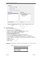
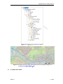
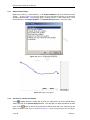
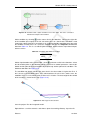
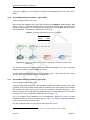
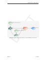
1D/2D/3D Modelling suite for integral water solutions
DR
AF
T
Delft3D Flexible Mesh Suite
D-Real Time Control
User Manual
DR
AF
T
T
DR
AF
D-Real Time Control
D-Real Time Control (D-RTC) in Delta Shell
User Manual
Version: 3.4.0
Revision: 41757
24 September 2015
DR
AF
T
D-Real Time Control, User Manual
Published and printed by:
Deltares
Boussinesqweg 1
2629 HV Delft
P.O. 177
2600 MH Delft
The Netherlands
For sales contact:
telephone: +31 88 335 81 88
fax:
+31 88 335 81 11
e-mail:
[email protected]
www:
http://www.deltaressystems.nl
telephone:
fax:
e-mail:
www:
+31 88 335 82 73
+31 88 335 85 82
[email protected]
https://www.deltares.nl
For support contact:
telephone: +31 88 335 81 00
fax:
+31 88 335 81 11
e-mail:
[email protected]
www:
http://www.deltaressystems.nl
Copyright © 2015 Deltares
All rights reserved. No part of this document may be reproduced in any form by print, photo
print, photo copy, microfilm or any other means, without written permission from the publisher:
Deltares.
Contents
Contents
.
.
.
.
.
.
.
.
.
.
.
.
.
.
.
.
.
.
.
.
.
.
.
.
.
.
.
.
.
.
.
.
.
.
.
.
.
.
.
.
.
.
.
.
.
.
.
.
.
.
.
.
.
.
.
.
.
.
.
.
.
.
.
.
.
.
.
.
.
.
.
.
.
.
.
.
.
.
.
.
.
.
.
.
.
.
.
.
.
.
1
1
1
1
1
2
2 Module D-RTC: Overview
2.1 Introduction . . . . . . . . . . . . . . . . .
2.2 Controlgroup . . . . . . . . . . . . . . . .
2.3 Flow chart . . . . . . . . . . . . . . . . .
2.4 The properties window . . . . . . . . . . .
2.5 Examples . . . . . . . . . . . . . . . . . .
2.5.1 Minimal controlflow . . . . . . . . .
2.5.2 Combinations of conditions and rules
.
.
.
.
.
.
.
.
.
.
.
.
.
.
.
.
.
.
.
.
.
.
.
.
.
.
.
.
.
.
.
.
.
.
.
.
.
.
.
.
.
.
.
.
.
.
.
.
.
.
.
.
.
.
.
.
.
.
.
.
.
.
.
.
.
.
.
.
.
.
.
.
.
.
.
.
.
.
.
.
.
.
.
.
.
.
.
.
.
.
.
.
.
.
.
.
.
.
.
.
.
.
.
.
.
.
.
.
.
.
.
.
.
.
.
.
.
.
.
3
3
5
6
6
7
7
8
3 Module D-RTC: Getting started
3.1 Introduction . . . . . . . . . . . . . . . . . . . . . .
3.2 Getting started . . . . . . . . . . . . . . . . . . . .
3.2.1 The integrated model . . . . . . . . . . . . .
3.2.2 The D-Flow 1D model . . . . . . . . . . . .
3.3 A simple D-RTC model . . . . . . . . . . . . . . . .
3.3.1 Add a Control Group . . . . . . . . . . . . .
3.3.2 Construct a minimal controlflow . . . . . . . .
3.3.3 Perform a simulation . . . . . . . . . . . . .
3.4 View the simulation results . . . . . . . . . . . . . .
3.4.1 Introduction . . . . . . . . . . . . . . . . . .
3.4.2 Table view . . . . . . . . . . . . . . . . . .
3.4.3 Side-view . . . . . . . . . . . . . . . . . . .
3.5 A more complex control flow . . . . . . . . . . . . .
3.5.1 Multiple controlled parameters on one structure
3.5.2 Multiple controlled structures . . . . . . . . .
3.6 Control flows with conditions . . . . . . . . . . . . .
3.6.1 A controlflow with a condition . . . . . . . . .
3.6.2 A controlflow with two conditions: logical AND
3.6.3 A controlflow with two conditions: logical OR .
.
.
.
.
.
.
.
.
.
.
.
.
.
.
.
.
.
.
.
.
.
.
.
.
.
.
.
.
.
.
.
.
.
.
.
.
.
.
.
.
.
.
.
.
.
.
.
.
.
.
.
.
.
.
.
.
.
.
.
.
.
.
.
.
.
.
.
.
.
.
.
.
.
.
.
.
.
.
.
.
.
.
.
.
.
.
.
.
.
.
.
.
.
.
.
.
.
.
.
.
.
.
.
.
.
.
.
.
.
.
.
.
.
.
.
.
.
.
.
.
.
.
.
.
.
.
.
.
.
.
.
.
.
.
.
.
.
.
.
.
.
.
.
.
.
.
.
.
.
.
.
.
.
.
.
.
.
.
.
.
.
.
.
.
.
.
.
.
.
.
.
.
.
.
.
.
.
.
.
.
.
.
.
.
.
.
.
.
.
.
.
.
.
.
.
.
.
.
.
.
.
.
.
.
.
.
.
.
.
.
.
.
.
.
.
.
.
.
.
.
.
.
.
.
.
.
.
.
15
15
15
15
16
17
18
18
19
19
19
19
20
20
21
22
23
24
26
26
4 Module D-RTC: All about the modelling process
4.1 Conditions . . . . . . . . . . . . . . . . .
4.1.1 Hydro condition . . . . . . . . . . .
4.1.2 Time condition . . . . . . . . . . .
4.2 Rules . . . . . . . . . . . . . . . . . . . .
4.2.1 Hydraulic rule . . . . . . . . . . . .
4.2.2 Time rule . . . . . . . . . . . . . .
4.2.3 PID rule . . . . . . . . . . . . . .
4.2.3.1 Introduction . . . . . . .
4.2.3.2 PID rules in D-RTC . . . .
4.2.3.3 PID rule calibration . . . .
4.2.4 Interval rule . . . . . . . . . . . . .
4.2.5 Relative from time/value rule . . . .
.
.
.
.
.
.
.
.
.
.
.
.
.
.
.
.
.
.
.
.
.
.
.
.
.
.
.
.
.
.
.
.
.
.
.
.
.
.
.
.
.
.
.
.
.
.
.
.
.
.
.
.
.
.
.
.
.
.
.
.
.
.
.
.
.
.
.
.
.
.
.
.
.
.
.
.
.
.
.
.
.
.
.
.
.
.
.
.
.
.
.
.
.
.
.
.
.
.
.
.
.
.
.
.
.
.
.
.
.
.
.
.
.
.
.
.
.
.
.
.
.
.
.
.
.
.
.
.
.
.
.
.
.
.
.
.
.
.
.
.
.
.
.
.
29
29
29
30
31
32
33
34
34
35
36
37
38
DR
AF
T
1 A guide to this manual
1.1 Introduction . . . . . . . . . . . . . . . .
1.2 Overview . . . . . . . . . . . . . . . . .
1.3 Manual version and revisions . . . . . . .
1.4 Typographical conventions . . . . . . . .
1.5 Changes with respect to previous versions
5 Module D-RTC: Simulation and model output
Deltares
.
.
.
.
.
.
.
.
.
.
.
.
.
.
.
.
.
.
.
.
.
.
.
.
.
.
.
.
.
.
.
.
.
.
.
.
.
.
.
.
.
.
.
.
.
.
.
.
.
.
.
.
.
.
.
.
.
.
.
.
39
iii
D-Real Time Control, User Manual
41
DR
AF
T
References
iv
Deltares
List of Figures
List of Figures
.
.
.
.
.
.
.
.
.
.
.
.
.
.
.
.
.
.
.
.
.
.
.
.
.
.
.
.
.
.
.
.
.
.
.
.
.
.
.
.
.
.
.
.
.
.
.
.
.
.
.
.
.
.
.
.
.
.
.
.
.
.
.
.
.
.
.
.
T
Example of an RTC-model in the project explorer . . . . . . .
Example of a flow chart . . . . . . . . . . . . . . . . . . . .
Example of the properties window for a Time rule . . . . . . .
D-RTC modelling concept and data flow . . . . . . . . . . . .
Components and basic concept of the flowchart . . . . . . . .
Example minimal controlflow . . . . . . . . . . . . . . . . .
Example minimal controlflow with a condition . . . . . . . . .
Example of two conditions that combined form an AND trigger
Example of two conditions that combined form an OR trigger .
Example of three conditions: 1 AND (2 OR 3) . . . . . . . . .
Example of three conditions: 1 OR (2 AND 3) . . . . . . . . .
Example of four conditions: 4 OR (1 AND 2 AND 3) . . . . . .
Example of four conditions: 1 AND 2 AND (3 OR 4) . . . . . .
Example of four conditions: (1 OR 2) AND (3 OR 4) . . . . . .
Example of four conditions: (1 AND (3 OR 4)) OR (2 AND 4) .
Example of four conditions: 4 AND (1 OR 2 OR 3) . . . . . .
Example of four conditions: (1 AND 2) OR (3 AND 4) . . . . .
.
.
.
.
.
.
.
.
.
.
.
.
.
.
.
.
.
.
.
.
.
.
.
.
.
.
.
.
.
.
.
.
.
.
.
.
.
.
.
.
.
.
.
.
.
.
.
.
.
.
.
.
.
.
.
.
.
.
.
.
.
.
.
.
.
.
.
.
DR
AF
2.1
2.2
2.3
2.4
2.5
2.6
2.7
2.8
2.9
2.10
2.11
2.12
2.13
2.14
2.15
2.16
2.17
3
4
4
5
7
8
8
8
9
9
10
10
11
11
12
12
13
15
3.21
Integrated model default properties . . . . . . . . . . . . . . . . . . . .
Integrated model, settings for a coupled simulation with D-RTC and D-Flow 1D
. . . . . . . . . . . . . . . . . . . . . . . . . . . . . . . . . . . . . . . .
Integrated model in the project Explorer . . . . . . . . . . . . . . . . . . . .
Example water flow model schematisation with an OpenStreet background
map (http://openstreetmap.org) . . . . . . . . . . . . . . . . . . . . .
Options for default controlgroups . . . . . . . . . . . . . . . . . . . . . . .
Empty controlgroup . . . . . . . . . . . . . . . . . . . . . . . . . . . . . .
Minimum flow chart with a Time Rule . . . . . . . . . . . . . . . . . . . . .
Project Explorer after a coupled simulation with D-RTC and D-Flow 1D. . . .
Table and chart view D-RTC output . . . . . . . . . . . . . . . . . . . . . .
Sideview with water level, discharge and crest level of the structure . . . . . .
Flowchart for example with two controlled parameters for one weir. . . . . . .
Structure selected on the map view of simulation output . . . . . . . . . . . .
Select output coverage . . . . . . . . . . . . . . . . . . . . . . . . . . . .
Crest level, crest width and water level over time for the weir. A point in time
has been selected in the diagram, the corresponding line is selected in the table.
Chart properties window, the chart title “Simulation results” has been added. .
D-Flow 1D network with two weirs. . . . . . . . . . . . . . . . . . . . . . .
D-Flow 1D network with one weir and a single observation point upstream. . .
Flowchart with a Hydro Condition and a Time Rule. The rule is connected with
the true-output of the condition. . . . . . . . . . . . . . . . . . . . . . . . .
Data origin for the structure . . . . . . . . . . . . . . . . . . . . . . . . . .
Flowchart with two Hydro conditions in an AND combination combined with a
Time rule. . . . . . . . . . . . . . . . . . . . . . . . . . . . . . . . . . . .
Flowchart with two Hydro conditions in an OR combination and a Time rule. . .
4.1
4.2
4.3
4.4
4.5
4.6
4.7
Example of a flowchart with a hydro condition
A hydro condition in the Properties Window
Example of a flowchart with a time condition
A time condition in the Properties Window .
A hydraulic rule in the flowchart . . . . . . .
A hydraulic rule in the Properties Window .
A time rule in the flowchart . . . . . . . . .
30
30
31
31
32
33
33
3.1
3.2
3.3
3.4
3.5
3.6
3.7
3.8
3.9
3.10
3.11
3.12
3.13
3.14
3.15
3.16
3.17
3.18
3.19
3.20
Deltares
.
.
.
.
.
.
.
.
.
.
.
.
.
.
.
.
.
.
.
.
.
.
.
.
.
.
.
.
.
.
.
.
.
.
.
.
.
.
.
.
.
.
.
.
.
.
.
.
.
.
.
.
.
.
.
.
.
.
.
.
.
.
.
.
.
.
.
.
.
.
.
.
.
.
.
.
.
.
.
.
.
.
.
.
.
.
.
.
.
.
.
.
.
.
.
.
.
.
.
.
.
.
.
.
.
.
.
.
.
.
.
.
.
.
.
.
.
.
.
16
17
17
18
18
19
20
20
21
21
22
22
23
23
24
24
25
25
26
27
v
D-Real Time Control, User Manual
4.8
4.9
4.10
4.11
4.12
A time rule in the Properties Window . .
A PID rule in the flowchart . . . . . . . .
A PID rule in the Properties Window . . .
An interval rule in the flowchart . . . . . .
An interval rule in the Properties Window
5.1
D-RTC-model selected in the Project Explorer . . . . . . . . . . . . . . . . 39
.
.
.
.
.
.
.
.
.
.
.
.
.
.
.
.
.
.
.
.
.
.
.
.
.
.
.
.
.
.
.
.
.
.
.
.
.
.
.
.
.
.
.
.
.
.
.
.
.
.
.
.
.
.
.
.
.
.
.
.
.
.
.
.
.
.
.
.
.
.
.
.
.
.
.
.
.
.
.
.
.
.
.
.
.
34
35
36
37
38
DR
AF
T
.
.
.
.
.
vi
Deltares
List of Tables
List of Tables
Discharge boundary condition table for the upstream end
Time Rule data for crest level . . . . . . . . . . . . . .
Time series for the crest width (rule 2) . . . . . . . . .
Time series of crest level for a second structure . . . . .
Parameter-Data table for condition . . . . . . . . . . .
Parameter-Data table for the second condition . . . . .
.
.
.
.
.
.
.
.
.
.
.
.
.
.
.
.
.
.
.
.
.
.
.
.
.
.
.
.
.
.
.
.
.
.
.
.
.
.
.
.
.
.
.
.
.
.
.
.
.
.
.
.
.
.
.
.
.
.
.
.
.
.
.
.
.
.
16
19
21
24
25
26
4.1
Example hydraulic rule for structure . . . . . . . . . . . . . . . . . . . . . . 32
DR
AF
T
3.1
3.2
3.3
3.4
3.5
3.6
Deltares
vii
DR
AF
T
D-Real Time Control, User Manual
viii
Deltares
1 A guide to this manual
1.1
Introduction
This User Manual concerns the module D-Real Time Control.
This module is part of several Modelling suites, released by Deltares as Deltares Systems
or Dutch Delta Systems. These modelling suites are based on the Delta Shell framework.
The framework enables to develop a range of modeling suites, each distinguished by the
components and — most significantly — the (numerical) modules, which are plugged in. The
modules which are compliant with the Delta Shell framework are released as D-Name of the
module, for example: D-Flow Flexible Mesh, D-Waves, D-Water Quality, D-Real Time Control,
D-Rainfall Run-off.
1.2
DR
AF
T
Therefore, this user manual is shipped with several modelling suites. In the start-up screen
links are provided to all relevant User Manuals (and Technical Reference Manuals) for that
modelling suite. It will be clear that the Delta Shell User Manual is shipped with all these
modelling suites. Other user manuals can be referenced. In that case, you need to open the
specific user manual from the start-up screen in the central window. Some texts are shared
in different user manuals, in order to improve the readability.
Overview
To make this manual more accessible we will briefly describe the contents of each chapter.
If this is your first time to start working with D-RTC we suggest you to read Chapter 3, Module
D-RTC: Getting started. This chapter provides a tutorial.
Chapter 2: Module D-RTC: Overview, gives a brief introduction on D-RTC.
Chapter 3: Module D-RTC: Getting started, provides examples of D-RTC with a tutorial.
Chapter 4: Module D-RTC: All about the modelling process, provides practical information
on the GUI, setting up so-called Control groups presented as a Flow chart and validating the
model.
Chapter 5: Module D-RTC: Simulation and model output, describes how the simulation results
can be accessed.
1.3
Manual version and revisions
This manual applies to SOBEK 3 suite (version 3.4) and Delft3D Flexible Mesh (version 2015).
1.4
Typographical conventions
Throughout this manual, the following conventions help you to distinguish between different
elements of text.
Deltares
1 of 44
D-Real Time Control, User Manual
Description
Waves
Boundaries
Title of a window or sub-window.
Sub-windows are displayed in the Module window and
cannot be moved.
Windows can be moved independently from the Module window, such as the Visualisation Area window.
Save
Item from a menu, title of a push button or the name of
a user interface input field.
Upon selecting this item (click or in some cases double
click with the left mouse button on it) a related action
will be executed; in most cases it will result in displaying
some other (sub-)window.
In case of an input field you are supposed to enter input
data of the required format and in the required domain.
<\tutorial\wave\swan-curvi>
<siu.mdw>
Directory names, filenames, and path names are expressed between angle brackets, <>. For the Linux
and UNIX environment a forward slash (/) is used instead of the backward slash (\) for PCs.
DR
AF
T
Example
“27 08 1999”
Data to be typed by you into the input fields are displayed between double quotes.
Selections of menu items, option boxes etc. are described as such: for instance ‘select Save and go to
the next window’.
delft3d-menu
Commands to be typed by you are given in the font
Courier New, 10 points.
User actions are indicated with this arrow.
[m/s] [-]
1.5
Units are given between square brackets when used
next to the formulae. Leaving them out might result in
misinterpretation.
Changes with respect to previous versions
This edition has only minor adjustments.
2 of 44
Deltares
2 Module D-RTC: Overview
Introduction
The D-RTC (Real Time Control) plug-in can be used for the simulation of real time control
of hydraulic systems. It can be applied to rainfall-runoff, hydraulics and water quality computations. The D-RTC module is used in a composite model and is always combined to a
hydrodynamic model, such as D-Flow 1D and/or D-RR and/or D-WAQ. A D-RTC model has
three main windows in Delta Shell: the Project Explorer, the map with the Flow chart, and
the Properties Window.
T
The Project Explorer is used to show a total overview of all D-RTC model objects, while the
map and flow chart show the relations between the D-RTC components. Figure 2.1 shows
an example of a D-RTC-model in the Project Explorer. In this case the composite model
contains a D-Flow 1D model and the D-RTC model. The D-RTC model consists of a set of
controlgroups and an output folder. This is described in more detail in section 2.2. Figure 2.2
shows an example of a flowchart. Flowcharts are described in section 2.3. The Properties
window shows details of the RTC-components and facilitates editing (see also section 2.4).
Figure 2.3 shows an example of the Properties Window for a Time rule (see also ??).
DR
AF
2.1
Figure 2.1: Example of an RTC-model in the project explorer
Deltares
3 of 44
DR
AF
T
D-Real Time Control, User Manual
Figure 2.2: Example of a flow chart
Figure 2.3: Example of the properties window for a Time rule
Figure 2.4 gives an overview of the RTC modelling concept. D-RTC uses observed values of
control parameters to determine the values of controlled parameters. These observed values
can consist of actual measurements or observations from the hydrodynamic model. Examples
of control parameters are:
Hydraulic parameters at an observation point, such as discharge or waterlevel
Water quality parameters at an observation point
Rainfall
External data, such as meteorological conditions, diversions due to building or maintenance activities etc.
Controlled parameters are positions of moving elements of the structures that are directed by
D-RTC. Examples are
Crest level or crest width of weirs
Discharge of pumps
4 of 44
Deltares
Module D-RTC: Overview
T
Gate opening at gated weirs
Valve opening at Culverts
DR
AF
Figure 2.4: D-RTC modelling concept and data flow
D-RTC uses the input from control parameters to evaluate conditions that trigger rules that set
the controlled parameters. For example, if a pump operates during the night with a capacity
of 500 m3 /s and is shut down during the day, the condition is true during the night and false
during the day. The rule connected to the "true" output sets the discharge to 500 m3 /s, while
the rule connected to "false" output set the discharge of the pump to 0 m3 /s.
Rules contain the actual algorithms that D-RTC uses to calculate the values of a controlled
parameter.
Conditions trigger a rule to be active or not. Both the true and false outcome of a condition
can be used to activate rules.
By connecting a sequence of conditions and rules, a control flow is generated for a controlled
parameter. This controlflow is visualized in a flowchart, which is described in more detail
below.
D-RTC uses the objects from a hydraulic model such as a D-Flow 1D model, but has no
knowledge of the model itself and no spatial information. The objects from a hydraulic model
used by D-RTC are passive objects which can not be edited in D-RTC. D-RTC directs the
controlflow, which means that the only editable objects are rules and conditions.
2.2
Controlgroup
A D-RTC model consists of one or multiple controlgroups which are shown in the Project
Explorer. A controlgroup is a set of D-RTC components. Each controlgroup consists of
one flow chart with one ore more controlflows (see section 2.3)
a list of observation points which supply the values of the control parameters
a list of conditions used in the controlflow(s)
a list of rules used in the controlflow(s)
a list of structure output locations for the controlled parameters
The set of elements in a single flowchart is a single controlgroup and one or more control-
Deltares
5 of 44
D-Real Time Control, User Manual
groups form a D-RTC model.
The controlgroup can be used to organize the D-RTC model. For example, a user can decide
to group the controlflows per
controlled parameter; each controlled parameter has its own controlflow and a controlgroup has one controlflow,
controlled structure; a controlled structure can have controlflows for each controlled pa-
T
rameter (for example, both crest level and crest width are controlled of a single weir). Each
controlgroup can then have more than one controlflow,
compound structure; several structures combined can form one large complex, such as
Haringvlietsluizen, which consist of 17 individual locks. It can be convenient to group DRTC around these compound structures. Each controlgroup can then contain more than
one controlflow, one for each controlled parameter.
2.3
DR
AF
Deciding how to group the controlflows is finding a balance between transparancy and easier
modeling in the controlgroups, and having a good overview of the total model. It is recommended to use as few controlflows as possible within a single controlgroup. Only use more
than one controlflow per controlgroup if the project explorer becomes too complex.
Flow chart
The flow chart is the visual interpretation of the controlgroup. While the Project Explorer only
shows a list of all components of a controlgroup, the flowchart shows how the components of
the controlgroup relate to one another.
D-RTC is built around the concept of controlflows. Figure 2.5 shows the concept of a controlflow and its components. The controlflow in a flow chart always:
has one starting point for each controlled parameter (depicted with a thick black line
around the controlflow component, see Figure 2.5),
has at least one controlled parameter and one rule,
can combine multiple conditions and rules,
shows the controlflow with solid arrows, and data input or output with dashed arrows, see
Figure 2.5,
has exactly one active path per controlled parameter (no 2 rules for the same controlled
parameter are active at the same time).
In section 2.5 examples are described in more detail.
The properties window
Similarly to other Delta Shell modules in D-RTC the Properties window shows details of a DRTC schematisation object by clicking on an item in the Project Explorer or on the flowchart.
The corresponding parameters can be edited in this window. An additional table window is
shown if necessary. Examples for properties of different D-RTC objects are given below:
Condition parameters:
condition type
the table in case of a lookup table controller
control parameters:
2.4
6 of 44
discharge
waterlevel
Deltares
Module D-RTC: Overview
salinity
rule type
the table of a lookup table controller
rule-specific parameters
DR
AF
T
controlled locations and parameters
Rule parameters:
Figure 2.5: Components and basic concept of the flowchart
2.5
Examples
In this section several examples of controlflows are presented. These examples also form the
basis for the tutorial in ??.
2.5.1
Minimal controlflow
Figure 2.6 shows the minimal controlflow; a parameter controlled by a rule. Depending on
the type of rule, there may be also be control data required. In addition to a rule, conditions
can be added that (de)activate a rule, Figure 2.7. An example for Figure 2.6 could be that the
water level is 3 m on the first day and 6 m on day two at a specified location. A condition for
that rule is added in Figure 2.7 and could imply that the rule is only active when the discharge
at a certain observation point is higher than a specified value. ?? explains which types of
rules and conditions are available and what they do.
Deltares
7 of 44
D-Real Time Control, User Manual
T
Figure 2.6: Example minimal controlflow
Figure 2.7: Example minimal controlflow with a condition
Combinations of conditions and rules
DR
AF
2.5.2
In this section an overview is given of basic combinations of conditions and rules.
A condition can be used on its own, but will often be used in combinations. The most elementary combinations of two conditions are AND and OR. An AND combination of two conditions
means that both conditions have to be true for the rule to be active. As soon as one of the two
conditions is false, the rule becomes inactive. The controlflow first checks the first condition,
and only if this condition is true, the controlflow proceeds to check the second condition. If
either the first or second condition is false, another rule can be activated. It is not required to
have a different rule for the false-scenario; if a structure only has to perform an action if the
conditions are true, no second rule is required. A second rule is only required if the structure
also has to perform an action once the conditions are false.
An OR combination of two conditions means that only one of the two conditions has to be true
for the rule to be active. Only if both conditions are false, the rule becomes inactive.
Figure 2.8: Example of two conditions that combined form an AND trigger
8 of 44
Deltares
DR
AF
T
Module D-RTC: Overview
Figure 2.9: Example of two conditions that combined form an OR trigger
By adding conditions the controlflow may be expanded to more complex situations. Figures
2.10 and 2.11 show some possibilites by using three conditions in a single controlflow. All
possibilities for combinations of three conditions are:
1 AND 2 AND 3
1 OR 2 OR 3
1 AND (2 OR 3) (Figure 2.10)
1 OR (2 AND 3) (Figure 2.11)
Figure 2.10: Example of three conditions: 1 AND (2 OR 3)
Deltares
9 of 44
DR
AF
T
D-Real Time Control, User Manual
Figure 2.11: Example of three conditions: 1 OR (2 AND 3)
Similarly, the control flow can be extended with even more conditions and rules. Figures 2.12
to 2.17 give examples for a situation with four conditions.
Figure 2.12: Example of four conditions: 4 OR (1 AND 2 AND 3)
10 of 44
Deltares
DR
AF
T
Module D-RTC: Overview
Figure 2.13: Example of four conditions: 1 AND 2 AND (3 OR 4)
Figure 2.14: Example of four conditions: (1 OR 2) AND (3 OR 4)
Deltares
11 of 44
DR
AF
T
D-Real Time Control, User Manual
Figure 2.15: Example of four conditions: (1 AND (3 OR 4)) OR (2 AND 4)
Figure 2.16: Example of four conditions: 4 AND (1 OR 2 OR 3)
12 of 44
Deltares
DR
AF
T
Module D-RTC: Overview
Figure 2.17: Example of four conditions: (1 AND 2) OR (3 AND 4)
Note the difference between Figures 2.14 and 2.15; there is only a small difference in flowchart
(the arrow going from the true side of Condition 2 to Condition 3), but a large difference in
meaning!
Deltares
13 of 44
DR
AF
T
D-Real Time Control, User Manual
14 of 44
Deltares
3 Module D-RTC: Getting started
3.1
Introduction
In this chapter we will provide examples of D-RTC with a tutorial. The D-RTC module can not
be used on its own: an RTC model uses information and determines the values of parameters
of another model, typically a D-Flow 1D model or D-Flow FM model. However, this can also
be a water quality model or a rainfall-runoff model. We start with the tutorial model of D-Flow
1D.
The integrated model
Applying control with D-RTC on a D-Flow 1D model is coupled modeling or integrated modeling. To develop an integrated model in Delta Shell right-mouse click on the project, e. g.
<project1>, in the Project Explorer. Select Add. . . and choose New Model . . . . A Select
model . . . dialog appears. Choose “Integrated Model”. In the central window the integrated
model dialog appears (Figure 3.1). Under Models and Tools delete all items but “real-time
control” and “water flow 1d” with the Delete button. Set the Run Parameters in such a way
that the simulation period begins on 2000-01-01 and ends on 2000-01-05. Set the time step
to one hour. The window should now look like the one in Figure 3.2.
T
3.2.1
Getting started
DR
AF
3.2
Figure 3.1: Integrated model default properties
The Project Explorer now looks like Figure 3.3. The <Region> folder contains schematisations for the models: a network for the D-Flow 1D model and a basin for rainfall-runoff models.
The latter one is not used in this tutorial. Under <Models> we find the D-Flow 1D-model
“water flow 1d” and the D-RTC model “real-time control”. Note that the network of the water
flow 1d model is a link to the network under <Region>.
Deltares
15 of 44
DR
AF
T
D-Real Time Control, User Manual
Figure 3.2: Integrated model, settings for a coupled simulation with D-RTC and DFlow 1D
3.2.2
The D-Flow 1D model
Create a simple D-Flow 1D model:
(Optional) Enable OpenStreetMap WMS layer
Add one branch with a length of about 60 km long to the network.
Add a cross-section of type YZ with default properties.
Add a Weir node with default properties.
Create a computational grid.
Set a constant water level of -2 m at the downstream boundary.
Set a transient discharge boundary condition at the upstream end (Table 3.1).
Set the current crest level the current crest width of structures as output parameter.
Set the current water level and the current discharge of observation points as output parameter.
Save the project.
Validate the model.
Run the model.
The flow model schematisation (<network>) then should look more or less like the one given
with Fig. 3.4.
Table 3.1: Discharge boundary condition table for the upstream end
Date
2000-01-01 00:00:00
2000-01-02 00:00:00
2000-01-05 00:00:00
16 of 44
Discharge in m3 /s
300
300
500
Deltares
DR
AF
T
Module D-RTC: Getting started
Figure 3.3: Integrated model in the project Explorer
Figure 3.4: Example water flow model schematisation with an OpenStreet background
map (http: // openstreetmap. org )
3.3
A simple D-RTC model
Deltares
17 of 44
D-Real Time Control, User Manual
3.3.1
Add a Control Group
DR
AF
T
Right-mouse click on <Control Groups> in the Project Explorer and select Add New Control
Group. . . . A menu (Figure 3.5) appears where the user can choose between a set of default
available control groups. Select empty group. Control Group 1 is now added to the set of
Control Groups in the Project Explorer. The Control Group window is currently empty.
Figure 3.5: Options for default controlgroups
Figure 3.6: Empty controlgroup
3.3.2
Construct a minimal controlflow
Select
(toolbar below the empty flow chart on the right-hand side of the Control Group
editor) and click in the Control Group window. This tool adds an output location to the flow
chart. Select
under the flow chart and click in the flow chart to add a rule. Connect the two
objects to obtain a flow chart as shown in Figure 3.7: move the mouse over the rule object,
18 of 44
Deltares
Module D-RTC: Getting started
Table 3.2: Time Rule data for crest level
Date
2000-01-01 00:00:00
2000-01-02 00:00:00
2000-01-05 00:00:00
Crest level in m
1
1
-8
T
left-click on the anchor point of the rule object on its right side, hold the mouse clicked and
find the anchor point on the left side of the output location object. Release the mouse button.
Figure 3.7: Minimum flow chart with a Time Rule
DR
AF
Now set the crest level of the weir as output location: right-click click on the output location
object and navigate through the menus. From the available locations in the network of the
flow model select the weir as location and crest level as controlled parameter. The output
location ellipsoid turns blue after having specified the parameters. Note that now in the map
the available location are highlighted.
The default rule is a PID rule. In this tutorial we use a Time rule, because this is the simplest
one. Right-mouse click on the rule and select Convert PID Rule to Time Rule. The data of the
time rule can be edited in the Properties window. Under Data click on <Time Series> and
the drop down menu to open the table editor. Fill in the data from Table 3.2. Use the arrow
keys to switch between cells and the return key to add a new line. With the F2 key you can
address the date value. Select periodicity constant and interpolation linear (default values).
Save the project.
3.3.3
Perform a simulation
To perform a coupled flow simulation right-click on the <integrated model> in the Project
Explorer and choose Run Model.
3.4
3.4.1
View the simulation results
Introduction
Both the D-Flow 1D model and RTC run simultaneously and exchange data with each other
during run-time on a time stap basis. Figure 3.8 shows the Project Explorer after the simulation run. Both D-RTC and D-Flow 1D generate their own output; the output time step of
the D-Flow 1D model is set by the user. The RTC model uses this time step and puts out the
values of the controlled parameters per timestep. Note that the output of D-RTC is the input
for the next timestep D-Flow 1D computes.
3.4.2
Table view
Double click on <real-time control> <output> <crest level (s)> in the Project Explorer
(Figure 3.8) and select table and chart view. A tab opens in which the crest levels are shown
as a function of time (Figure 3.9). A mouse-click on the top left corner of the table selects the
Deltares
19 of 44
D-Real Time Control, User Manual
T
content. The data can now be copied and pasted to a file.
DR
AF
Figure 3.8: Project Explorer after a coupled simulation with D-RTC and D-Flow 1D.
Figure 3.9: Table and chart view D-RTC output
3.4.3
Side-view
To create a side-view double-click on <input> <network> in the water flow model to open
the network editor. Select
in the ribbon and click in the map to create a network
route along the branch. For this purpose, click on the start of the branch (the most upstream
point) and click on the end of the branch (most downstream point). A route between the two
points is created. The created route can be deleted in Region Contents under <network>
<Routes>. Click
in the ribbon to open the sideview. Right-mouse click in the side-view.
Select Select Coverages. Choose “Discharge” and “Crest level (s)” from the list. Navigate
through the time steps with the time series navigator to explore the simulation results in time
along the chainage of the channel.
3.5
A more complex control flow
20 of 44
Deltares
DR
AF
T
Module D-RTC: Getting started
Figure 3.10: Sideview with water level, discharge and crest level of the structure
3.5.1
Multiple controlled parameters on one structure
Save the project under a new name. Open the editor for Control Group 1. Select
in the flow chart to add an output location. Select
Connect the two objects.
and click
and click in the flow chart to add a rule.
Select the output location and right-mouse click to specify Weir1 as location and crest width
as controlled parameter. Select the new rule and right-mouse click to convert the standard
PID rule into a Time rule. Fill in the values from Table 3.3 under TimeSeries in the properties
window. The flow chart now looks as in Figure 3.11.
Table 3.3: Time series for the crest width (rule 2)
Date
2000-01-01 00:00:00
2000-01-02 00:00:00
2000-01-05 00:00:00
Crest width in m
5
5
20
Figure 3.11: Flowchart for example with two controlled parameters for one weir.
Run the integrated model again. Save the project. In addition to <crest level>, also <crest
width> is now available under <Output> of the real-time control model in the Project Ex-
Deltares
21 of 44
D-Real Time Control, User Manual
plorer.
To visualize the simulation results coherently, double click on <water flow model> <Output>
<water level>. If the structure feature is not visible in the map, change the view in the Map
DR
AF
T
Contents window: switch layers on or off or drag the network layer on top. Select the structure
feature on the map (Figure 3.12).
Figure 3.12: Structure selected on the map view of simulation output
Figure 3.13: Select output coverage
Then select the Query Time Series tool
. Press the Control key on your keyboard and
choose crest level, crest width and water level from the water flow 1d model as output coverage (Figure 3.13). These parameters are now plotted over time for the selected Weir Node
(Figure 3.14). Click with the mouse in the diagram or select rows in the table.
Add a title for the chart in the chart Properties window (Figure 3.15).
3.5.2
Multiple controlled structures
Save the project under a new name. Add a second weir to the network of the water flow
model. The network should now look like the one given in Figure 3.16. Change the crest
width to 30 m and the crest level to -4 m.
22 of 44
Deltares
T
Module D-RTC: Getting started
DR
AF
Figure 3.14: Crest level, crest width and water level over time for the weir. A point in time
has been selected in the diagram, the corresponding line is selected in the
table.
Figure 3.15: Chart properties window, the chart title “Simulation results” has been added.
Add a new control group to the D-RTC model: right-click on <Control Groups> in the Project
Explorer and select empty group. Add an output location and a Time Rule to the new Control
Group (buttons
and
, convert to Time Rule). Note that the name of the rule is rule01.
This name is also used in the first Control Group. Within one Control Group the names have
to be unique.
Fill in the table of the Time Rule properties with the data from Table 3.4. Select the output
location and set it to Weir2 and Crest level. Run the integrated model. Save the project.
Double-click on <crest level> in the Project Explorer under <real time control> <output>
and select Table and Chart View to open the output for the crest levels. The output of both
weirs is now visible in the table. Select
to filter the individual weirs. Apply a custom filter
on the value column to find out when the crest level of Weir1 is lower than -6 m.
3.6
Control flows with conditions
Deltares
23 of 44
D-Real Time Control, User Manual
T
Figure 3.16: D-Flow 1D network with two weirs.
Table 3.4: Time series of crest level for a second structure
2000-01-01 00:00:00
2000-01-02 00:00:00
2000-01-05 00:00:00
3.6.1
Crest level m
DR
AF
Date
-4
-4
-9
A controlflow with a condition
Save the project under a different name. Add an observation point to the network with the
help of the Create Observation Point tool
in the ribbon to the in the upstream part of the
network, close to the upstream boundary. Remove the second weir. The network should now
look like Figure 3.17.
Figure 3.17: D-Flow 1D network with one weir and a single observation point upstream.
Remove Control Group 1 from the D-RTC model. Save the project.
Go to Control Group 2. Let the Rule control the crest level of the weir.
24 of 44
Deltares
Module D-RTC: Getting started
T
Figure 3.18: Flowchart with a Hydro Condition and a Time Rule. The rule is connected
with the true-output of the condition.
DR
AF
Add a condition by selecting
and a mouse-click in the flowchart. Connect the right-side
of the condition (true-output) to the left side of the time rule. Note that the condition is now
shown with a thick, black line instead of the rule, indicating that the controlflow now starts with
the condition instead of the rule. Select the condition and fill in the Properties window with
data from Table 3.5. This is a so-called Hydro Condition, which evaluates input data and puts
out true or false.
Table 3.5: Parameter-Data table for condition
Operation
Value
>
3
Add an input location to the Control Flow: select
and mouse-click in the flowchart. Select
the observation point as data location and the water level as control parameter. Connect the
bottom anchor point of the data location object to the top anchor point of the condition. The
flowchart now looks like Figure 3.18.
The condition now checks whether the water level in the observation is higher than 3 m. If
this is the case, the condition returns ’true’, which activates the rule. If this is not the case, the
condition ’false’ as result, which means that the rule is inactive. The data origin for the control
of the structure is shown on the map (Figure 3.19).
Figure 3.19: Data origin for the structure
Save the project. Run the integrated model.
Right-click on <real-time control> and choose Open last working directory. Open the file
Deltares
25 of 44
D-Real Time Control, User Manual
<timeseries_0000.csv> and analyze the output of the computational core of D-RTC (RTCTools)1 .
3.6.2
A controlflow with two conditions: logical AND
Save the project under a new name.
Add a new hydro condition to the flow chart and fill in the Properties window with the data
given in Table 3.6. Add a data location object, select the observation point and choose Discharge as control parameter. Connect the true-output of the new condition with the input of
the first condition. The flowchart now looks like Figure 3.20.
>
300
DR
AF
Operation
Value
T
Table 3.6: Parameter-Data table for the second condition
Figure 3.20: Flowchart with two Hydro conditions in an AND combination combined with
a Time rule.
This flow chart represents a logical AND combination of two conditions. The rule is only active
if both the first and the second condition are active.
Run the integrated model and analyze the simulation results. Check when the rule is active
and the status of the conditions during simulation time.
3.6.3
A controlflow with two conditions: logical OR
Save the project under a new name.
Select the connection between the two conditions and delete it with the Delete-key on your
keyboard. Connect the bottom anchor point of condition01 (the false-output of the condition
that evaluates the water level) to the left side of condition02 (evaluates discharge). Then
connect the right side anchor point of condition02 to the left anchor point of the rule. Arrange
the elements in such a way that the flowchart looks like Figure 3.21.
This is an example of two conditions in an OR combination. Whereas in Figure 3.20 both
conditions had to be true for the rule to be active, in Figure 3.21 only one of the two conditions
needs to be true for the rule to be active.
Run the integrated model, save the project and analyze the results.
1
Future versions of SOBEK will provide more features to analyze simulation results of D-RTC
26 of 44
Deltares
DR
AF
T
Module D-RTC: Getting started
Figure 3.21: Flowchart with two Hydro conditions in an OR combination and a Time rule.
Deltares
27 of 44
DR
AF
T
D-Real Time Control, User Manual
28 of 44
Deltares
4 Module D-RTC: All about the modelling process
4.1
Conditions
In D-RTC there are 2 types of conditions:
1 Hydro condition
2 Time condition
The hydro condition uses data to assess whether a rule should be active or not, while the time
rule uses a timetable and is therefore independent of data.
Hydro condition
T
Figure 4.1 shows an example of the use of a hydro condition in a flowchart. A hydro condition
always needs input data, which are connected to the condition at the top side. These data
are the control parameters and can be any parameter available at a control location, i.e. water
level, discharge, velocity, but also salt concentration or water temperature, depending on the
modules used.
DR
AF
4.1.1
Figure 4.2 shows the Properties Window for a hydro condition. A hydro condition has as
parameters:
input
Operation
Value
id
name
The input is equal to the selected control location and parameter (in this case waterlevel at
observation point 1). The value is the setpoint of the control parameter. The hydro condition
checks with the operation how the actual value of the control parameter relates to the setpoint.
In the example in Figure 4.2 the hydro condition checks if the waterlevel at the observation
point is larger than zero. If this is the case, the operation is true and the hydro condition is
also true. If this is not the case, the operation is false as is the hydro condition. The following
operations are available
> (larger)
< (smaller)
= (equal)
<> (not equal)
>= (larger or equal)
<= (smaller or equal)
If the hydro condition is true, the rule connected to the true side (right side of the condition) is
activated and the rule connected to the false side (bottom side of the condition) is deactivated.
Otherwhise, if the condition is false, the rule connected to the true side is deactivated and the
rule connected to the false side is activated.
The id is obligatory and unique for the control group in which it is used. The name is not
obligatory and not necessarily unique.
Deltares
29 of 44
T
D-Real Time Control, User Manual
DR
AF
Figure 4.1: Example of a flowchart with a hydro condition
Figure 4.2: A hydro condition in the Properties Window
4.1.2
Time condition
Figure 4.3 shows an example of the use of a time condition. The main difference in flowchart
compared to a hydro condition is the absence of input data. The time condition is independent
of simulation results or measurements. It only needs a time table in which is stated during
which time the condition is true or false.
Figure 4.4 shows the Properties Window for a time condition. A time condition has the
following parameters:
Time Series
Extrapolation (constant, periodic, none)
Id: obligatory, unique for each Control Group
Name: optional and not necessarily unique
a window pops up in which the time table can be
By clicking on Time Series and selecting
entered. For each time entry true or false can be checked. Between two consecutive entries
the value of the first time entry is maintained. If the condition is true, the rule connected to the
true (right) side of the condition is activated, otherwise deactivated. Similarly, if the condition
is false, the rule connected to the false (bottom) side of the condition is activated, otherwise
deactivated.
30 of 44
Deltares
Module D-RTC: All about the modelling process
The parameter extrapolation controls what happens outside the ranges of the defined timetable.
Three options are possible:
Constant: the first and last value of the timetable are used for each time before and after
the defined timetable respectively.
Periodic: the time table is repeated before its first and after its last time entry.
None: no extrapolation, before the first and after the last time entry no rules are triggered
DR
AF
T
and the value of the controlled parameter is unaffected by RTC.
Figure 4.3: Example of a flowchart with a time condition
Figure 4.4: A time condition in the Properties Window
4.2
Rules
In D-RTC there are five different types of rules:
Hydraulic rule
Time rule
PID rule
Interval rule
Relative from time/value rule
All rules will be discussed below.
Deltares
31 of 44
D-Real Time Control, User Manual
Hydraulic rule
The hydraulic rule can be used to operate a structure as a function of a control parameter,
such as waterlevel or discharge at an observation point. The rule operates according to a
table with a specified relation between the control parameter and the controlled parameter.
An example of such a table is Table 4.1.
Table 4.1: Example hydraulic rule for structure
Controlled parameter:
crest level of weir m AD
0
1
2
3
4
5
4
3
2
1
T
Control parameter:
water level at observation
point
DR
AF
4.2.1
Figure 4.5: A hydraulic rule in the flowchart
Figure 4.6 shows the Properties Window for the hydraulic rule. The following parameters
can be set:
Id: obligatory and unique for the control group
Name: not obligatory and not necessarily unique
TimeLag (always given in seconds)
Extrapolation: extrapolation of table. Always constant
Interpolation: interpolation of table (constant or linear)
Table: Table with relation between control parameter and controlled parameter
The time lag is the time difference between the control parameter and the controlled parameter. For example, if the time lag is 1 day (86400 s), the value of the controlled parameter is
determined by the value of the control parameter one day before. It is not a delay in response
of the structure!
If a time lag different to zero is applied, care must be taken for the initial phase of the simulation. Until a simulation period equal to the time lag is computed, no input data is available
for the hydraulic rule. So the rule gives no output and no controlled parameter is transferred
to the structure connected to the rule. Consequently, the structure is considered to be not
controlled by D-RTC. For the simulation the parameter value specified for the structure in the
corresponding D-Flow 1D menu (see ?? and ??) is used in this case. Hence, for modeling
studies where a time lag for a hydraulic rule is specified the user either has to
32 of 44
Deltares
Module D-RTC: All about the modelling process
take into account the lack of input data for control in the initial phase in the analysis of
results or
T
use initial conditions from restart (a state saved previously; see ??).
Time rule
The time rule is the simplest rule; the controlled parameter is defined explicitly as a function
of time. The time rule is therefore the only rule without input data from a control parameter.
Figure 4.7 shows an example of the use of the time rule in the flowchart.
Figure 4.7: A time rule in the flowchart
Figure 4.8 shows the time rule in the Properties Window. The time rule has the following
parameters:
Timeseries: timetable of the controlled parameter as a function of time
Interpolation: interpolation within the time table (linear or constant)
Periodicity: extrapolation of time table. The options are
4.2.2
DR
AF
Figure 4.6: A hydraulic rule in the Properties Window
Constant: the last value is maintained
Periodic: the table is repeated (both before and after the times in the table)
Id: obligatory and unique for the control group
Name: not obligatory and not necessarily unique
Deltares
33 of 44
D-Real Time Control, User Manual
4.2.3.1
PID rule
Introduction
The PID (proportional integral derivative) rule is a control loop feedback mechanism used to
operate a structure in such way that a specified hydraulic control parameter (e.g. water level
or discharge) is maintained. The control parameter can be the water level or the discharge at
a specified observation point in the network.
DR
AF
4.2.3
T
Figure 4.8: A time rule in the Properties Window
The PID rule uses three tuning parameters
the proportional gain Kp
the integral gain Ki and
the derivative gain Kd
which must be adjusted for each situation. By adjusting the values the user puts the emphasis
of the rule on current deviations from the setpoint of the control parameter (Kp ), previous
deviations (Kd ) and all previous deviations (Ki ). This allows the user to set the behavior of
the rule such that the structure responds fast or that the response is dampened by previous
events. Wheras the interval rule can become unstable with many fluctuations in the controlled
parameter, by optimizing the factors the PID rule can be stabilized.
The PID rule computes the new value of the control parameter w(t) for a time step t as
follows:
w(t) = w(t − 1) + Kp e(t) + Ki
t
X
e(t) + Kd [e(t) − e(t − 1)]
(4.1)
t=0
in which e denotes the deviation of the controlled variable (e.g. the discharge) defined by the
set point minus the computed value at the previous time step.
If necessary, the new value of the control parameter w(t) is adjusted to fit within the physical
limits of the structure (i.e. Minimum, MaxSpeed, Maximum).
Gain factors can be positive or negative. The choice of the sign depends on the type of the
control structure (e.g. crest level, crest width or gate lower edge level) and the location and
type of the hydraulic parameter (e.g. water level or discharge) that is controlled by the PID rule.
For example, consider a PID rule that at a bifurcation tries to maintain a constant discharge
34 of 44
Deltares
Module D-RTC: All about the modelling process
flowing into one branch by manipulating the crest level of a River weir located in the branch
that should receive this constant discharge. In case the discharge flowing into the branch of
which its discharge is controlled is too large, this means that the deviation e in the equation
above is negative (i.e. e = set point actual discharge < 0). From a hydraulic point of view the
crest level (W(t)) of the river weir is to be raised in order to reduce the discharge flowing into
the controlled branch. In order to achieve this, the Kp gain factor should be negative.
PID rules in D-RTC
T
Figure 4.9 shows an example of the use of a PID rule in the flowchart.
DR
AF
Figure 4.9: A PID rule in the flowchart
Figure 4.10 shows the PID rule in the Properties Window. The PID rule uses the following
parameters:
Setpoint: setpoint of control parameter
IsUsingConstantSetpoint: true if the setpoint is constant in time, false if the setpoint is
a function of time
ConstantSetpoint: value of the setpoint if IsUsingConstantSetpoint is true
Table: table with setpoints as a function of time if IsUsingConstantSetpoint is false
TableExtrapolation/Interpolation: Linear or block interpolation and constant or periodic
extrapolation
Gain factors: Kp , Ki and Kd .
Limits: Physical limits of the structure
4.2.3.2
Minimum: minimum value of the controlled parameter
Maximum: maximum value of the controlled parameter
MaxSpeed: maximum velocity with which the controlled parameter is adjusted
Id: obligatory and unique for the controlgroup
Name: not obligatory and not necessarily unique
Deltares
35 of 44
T
D-Real Time Control, User Manual
4.2.3.3
DR
AF
Figure 4.10: A PID rule in the Properties Window
PID rule calibration
The gain factors Kp , Ki , Kd must be calibrated for optimal performance of the PID rule. For
example the calibration can be carried out as follows:
Take Kd , Ki equal to zero, and increase the value of Kp gradually from a small value
until the solution starts to oscillate. The sign of Kp must be chosen dependent of the type
of structure and the chosen control parameter (see technical background below)
Next divide the resulting value of Kp in half and start increasing Ki with a factor times
Kp . Again the value of Ki is increased until oscillations appear. Kd remains equal to
zero
Finally increase the value of Kd (sign of Kd may be opposite of sign of Ki )
A strict procedure for this calibration cannot be presented, since the procedures and results
are dependent on the type of model.
Warning:
Import from SOBEK 2
The PID rule can behave differently from the PID controller in previous releases of
SOBEK (2.12.002 and lower). During the import of a schematization from SOBEK 2,
the gain factors are changed to fit better within the new PID rule. Nevertheless, after
import from SOBEK we recommend to calibrate the PID rule again to obtain reliable
results.
36 of 44
Deltares
Module D-RTC: All about the modelling process
Interval rule
The interval rule can be used to operate a structure in such a way that a specified hydraulic
parameter is maintained. This controlled parameter can be the water level at a specified
observation point in the network, the discharge at a specified observation point in the network.
Figure 4.11 shows an example of the use of an interval rule in the flowchart. An interval rule
always needs the input of a control parameter.
Figure 4.12 shows the Properties Window for an interval rule. There are several parameters
available for the interval rule:
Setpoints control parameter; this is either a constant set point or a timeseries. Once a
timeseries has been generated, this is used as set point
Interpolation: only used when set points as a function of time are available. The interpoconstant
linear
T
lation is between the values in the time-series for the set points. Possibilities are
Below/above limits: Values for controlled parameter when control parameter is above or
below the setpoint
DR
AF
4.2.4
Deadband: a region in which the interval rule does not respond to deviations in the control
parameter from the setpoint
Deadband Type: the deadband region can be defined absolute or as a percentage
IntervalType: fixed or variable
Fixedinterval or Maxspeed: one of the two depending on the IntervalType must be entered
When the interval type is set to fixed, the controlled parameter is adjusted with a fixed amount
each timestep. This fixed amount is the parameter FixedInterval. In this mode the value of
the controlled parameter is independent of the actual timestep. If the controlled parameter is
crest level of a weir and the FixedInterval is set to 1, the crest level will be adjusted with 1
meter every timestep (within the limits of the structure set by the values Below and Above),
regardless whether the timestep is a minute or an hour. It is up to the user to set an appropriate
value for the FixedInterval.
When the interval type is set to variable, the controlled parameter is adjusted with a velocity,
specified by the parameter Maxspeed. This velocity is a maximum velocity. D-RTC checks
whether within that timestep the limits of the structure are reached. If so, the actual adjustment
is smaller and hence also the actual velocity. In this mode, the actual adjustment of the
structure is a function of the timestep. If the timestep is twice as long, the adjustment will be
twice as large (within the limits of the structure).
Figure 4.11: An interval rule in the flowchart
Deltares
37 of 44
T
D-Real Time Control, User Manual
4.2.5
DR
AF
Figure 4.12: An interval rule in the Properties Window
Relative from time/value rule
The relative time rule can be used to specify the controlled parameter as a function of time,
where the time (in seconds) is given relative to the moment that the rule is activated for the first
time by a condition. When the rule is activated for the first time, the relative time table is made
absolute (= computational time + relative time), thereafter the rule starts at the top of the table
and continues downward until the rule is deactivated by a condition. The rule table will remain
absolute during the user-defined so called Start period. In case the rule is activated after this
start period has passed, the table will be made absolute again. Start period= 0, means that
the table is made absolute each and every time that the rule is activated. In case the user
defined value for d(value)/dt is too small to allow for the in the Table defined changes in control
parameter, D-RTC will divert from these defined parameter values in such way as to best fit
the overall table. d(value)/dt= 0, means that there is no restriction in change in parameter over
one time step. When it reaches the end of the table, the value of the controlled parameter is
kept constant at the last value.
The relative from value rule is similar, except that the table is started not at the top, but at the
value of the controlled parameter.
38 of 44
Deltares
5 Module D-RTC: Simulation and model output
The simulation results of D-RTC can be accessed as described in section 3.4. D-RTC Simulation results are also written into a temporary directory of the user’s local settings:
c:\Documents and Settings\<user>\Local Settings\Temp\
where <user> is a placeholder for the user’s name.
T
Right-click in the Project Explorer and choose Open last working directory to navigate to the
current working directory where the simulation input and output is stored. The file <timeseries_0000.csv>
contains the time series of all model objects of the D-RTC model as comma-separated value
table. This file can be easily opened and postprocessed with text editors or programs like
Microsoft Excel or Matlab in order to analyze the simulated values related to input and output
locations and the status of D-RTC objects coherently.
Furthermore, the following files can be found in the temporary directory:
<rtcDataConfig.xml>
<tcRuntimeConfig.xml>
<rtcToolsConfig.xml>
<state_import.xml>
<statePI.xml>
<timeseries_export.xml>
DR
AF
With this set of xml-files a complete RTC-Tools model is given. RTC-Tools is the computational
core of D-RTC and can be considered as the research version of D-RTC (see http://oss.
deltares.nl/web/rtc-tools for details). <diag.xml> and <state_export.xml> are RTCTools output files.
Figure 5.1: D-RTC-model selected in the Project Explorer
Deltares
39 of 44
DR
AF
T
D-Real Time Control, User Manual
40 of 44
Deltares
DR
AF
T
References
Deltares
41 of 44
DR
AF
T
D-Real Time Control, User Manual
42 of 44
Deltares
DR
AF
T
T
DR
AF
PO Box 177
2600 MH Delft
Boussinesqweg 1
2629 VH Delft
The Netehrlands
+31 (0)88 335 81 88
[email protected]
www.deltaressystems.nl