1
PROCESSOR, PAYLOAD, AND POWER SUBSYSTEM DEVELOPMENT OF THE
MISSAT-1 CUBESAT
by
Zachary Christian Puuwai Olaa Morgan
Samuel Liyang Di
Rana Roxanne Gordji
A thesis submitted to the faculty of The University of Mississippi in partial fulfillment of
the requirements of the Sally McDonnell Barksdale Honors College.
Oxford
May 2014
Approved by
___________________________________
Advisor: Professor Matthew Inman
___________________________________
Reader: Professor Richard Gordon
___________________________________
Reader: Professor John O’Haver
© 2014
Zachary Christian Puuwai Olaa Morgan
Samuel Liyang Di
Rana Roxanne Gordji
ALL RIGHTS RESERVED
ii
Abstract
This thesis details the development and programming of the processor subsystem,
camera payload, and power subsystem of the Mississippi Imaging Space Satellite
(MISSat-1). An overview of the hardware and software considerations necessary for the
processor subsystem is discussed. An explanation of microcontroller uses as well as real
time operating system fundamentals is also presented as it relates to MISSat-1. The
subsystem deals with varieties of peripheral integration and communication standards
among devices. The camera graphical user interface (GUI) was expanded with the
addition of functions that improve CubeSat image handling. Additionally, image
processing techniques and algorithms are considered to improve CubeSat images. This
work continues the camera payload work undertaken by University of Mississippi
electrical engineering students from previous years. This paper will then discuss the
design and analysis completed thus far for the power subsystem of the MISSat-1. Such
topics will include an in-depth solar panel investigation, which will lead to the selection
of the solar panels that will be used on the MISSat-1. The solar panel selection, along
with the other chosen subsystem components, will allow for the formation of the power
budget, which shows the breakdown of power usage for each subsystem. The power
budget will then be developed into a Matlab GUI. Finally, the power budget will be
further analyzed by comparing it to other satellite projects.
iii
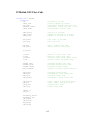
Table of Contents
LIST OF TABLES AND FIGURES ........................................................................................... vii
LIST OF ABBREVIATIONS .......................................................................................................x
1. INTRODUCTION..................................................................................................................1
2. PROCESSOR SUBSYSTEM ...................................................................................................3
I. Introduction ...................................................................................................................3
A. Project Description and Purpose..............................................................................3
II. Subsystem Overview ...................................................................................................5
A. General Requirements .............................................................................................5
B. Hardware Selection ..................................................................................................6
C. Software Selection ...................................................................................................7
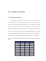
III. Development Configuration .....................................................................................11
A. Development Board Setup .....................................................................................11
B. PC Connection .......................................................................................................13
C. Integrated Development Environment ...................................................................15
IV. Peripheral Integration ...............................................................................................19
A. Serial Communication ...........................................................................................19
B. Payload...................................................................................................................21
C. Electrical Power System .......................................................................................28
D. Communication Board ...........................................................................................30
V. Conclusion .................................................................................................................33
3. PAYLOAD SUBSYSTEM ....................................................................................................34
I. Introduction .................................................................................................................34
A. Project Description and Purpose............................................................................34
B. Background Information ........................................................................................35
iv
II. CubeSat Cameras .......................................................................................................37
A. Survey of CubeSat Cameras ..................................................................................37
B. Camera Specifications ...........................................................................................38
III. Previous Work ..........................................................................................................40
A. Camera Selection ...................................................................................................40
B. Existing Code .........................................................................................................41
IV. Programming the Camera Interface .........................................................................43
A. Camera Operation ..................................................................................................43
B. Improvements and Modifications ..........................................................................43
V. Integration of Camera Interface into MISSat-1 .........................................................47
A. Space Imaging Conditions .....................................................................................47
B. Testing of Camera Settings ....................................................................................50
C. Image Processing ...................................................................................................51
VI. Conclusion ...............................................................................................................57
A. Future Work ...........................................................................................................57
4. POWER SUBSYSTEM ........................................................................................................59
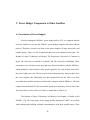
I. Introduction .................................................................................................................59
A. Project Description and Purpose............................................................................59
II. Solar Panels ...............................................................................................................60
A. Solar Cell Degradation ..........................................................................................60
B. EPS and Solar Panel Selection...............................................................................64
C. Overview of the EPS..............................................................................................66
III. Power Budget ...........................................................................................................69
A. Solar Panel Calculations ........................................................................................69
B. Modes of Operation ...............................................................................................71
C. Battery Charging ....................................................................................................75
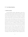
IV. Power Budget Simulations .......................................................................................77
A. Matlab Programming .............................................................................................77
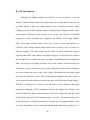
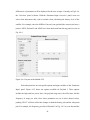
B. GUI Introduction....................................................................................................80
C. Simulation Results .................................................................................................82
v
V. Power Budget Comparison to Other Satellites ..........................................................85
A. Presentation of Power Budgets ..............................................................................85
B. Comparison ............................................................................................................91
VI. Conclusion ...............................................................................................................93
A. Future Work ...........................................................................................................93
5. APPENDIX .......................................................................................................................94
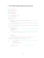
I. Salvo RTOS Sending and Receiving String Task .......................................................95
II. Camera GUI Code (C#) .............................................................................................96
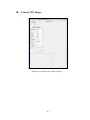
III. Camera GUI Image ..................................................................................................99
IV. Image Processing Code (Matlab) ...........................................................................100
V. Matlab GUI Code ....................................................................................................103
VI. Matlab GUI Class Code .........................................................................................115
6. LIST OF REFERENCES ....................................................................................................119
vi
List of Tables and Figures
Figure 1.1.1: Small satellite in low earth orbit ....................................................................1
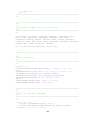
Figure 2.1.1: Microcontroller quad flat package ................................................................4
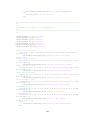
Figure 2.2.1: Single board computer motherboard .............................................................5
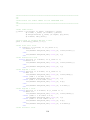
Figure 2.2.2: CubeSat Kit Pluggable Processor Module ....................................................6
Figure 2.2.3: RTOS program execution flow chart ............................................................9
Figure 2.2.4: Context switching among tasks ...................................................................10
Table 2.3.1: Development board test point voltage values ...............................................11
Table 2.3.2: USB powered test point voltage values ........................................................12
Table 2.3.3: HyperTerminal for program display .............................................................13
Figure 2.3.1: Program output in HyperTerminal ..............................................................14
Figure 2.3.2: Flash Emulation Tool for PC connections ..................................................16
Figure 2.3.3: MSP430 Flasher Command Line Programmer Interface ............................17
Figure 2.3.4: Flash Emulation Tool connection properties ...............................................18
Figure 2.4.1: UART character framing scheme ................................................................20
Table 2.4.1: Baud rates, settings, and errors .....................................................................21
Figure 2.4.2: On board camera pin layout ........................................................................22
Figure 2.4.3: Protoboard for CubeSat Kit bus connector scheme .....................................23
Figure 2.4.4: Synchronization signal sent from a laptop ..................................................24
Figure 2.4.5: Block diagram for transceiving with the development board .....................25
Figure 2.4.6: CrossStudio interface displaying successful receipt of signal .....................26
Figure 2.4.7: Camera interfacing work station .................................................................27
Figure 2.4.8: Synchronization signal sent from the development board ..........................28
Figure 2.4.9: Electrical power system connection pins ....................................................29
Figure 2.4.10: Data stored in Big versus Little Endianness ..............................................30
Figure 2.4.11: AstroDev Helium Radio product line board ..............................................31
Figure 2.4.12: Packet structure for commands and packet header description .................32
Figure 3.2.1: C6820 Module Specifications ......................................................................39
Figure 3.2.2: C6820 Dimensions .......................................................................................39
Figure 3.2.3: C6820 power measurements ........................................................................39
Figure 3.3.1: COMedia C6820...........................................................................................41
Figure 3.4.1: Table of transmission times ..........................................................................46
vii
Figure 3.5.1: Intelligent Space Systems Laboratory, University of Tokyo .......................48
Figure 3.5.2: Images taken by the COMPASS-1 CubeSat ................................................49
Figure 3.5.3: Calculated light intensity values seen by CubeSats .....................................50
Figure 3.5.4: Laplacian filter mask used for image sharpening .........................................51
Figure 3.5.5: Original image, Laplacian mask, and sharpened image ...............................52
Figure 3.5.6: Averaging and Gaussian filter mask, respectively .......................................53
Figure 3.5.7: Image, image blurred w/averaging, sharpened image, respectively.............53
Figure 3.5.8: Gaussian blurred image and sharpened image, respectively ........................53
Figure 3.5.9: Pixel value as a function of log exposure .....................................................56
Figure 4.2.1: Comparison of Solar Cell Materials .............................................................63
Table 4.2.1: Solar Cell Data used in the HESP Experiment ..............................................63
Figure 4.2.2: Comparison of Solar Cell Thicknesses ........................................................64
Table 4.2.2: Comparison of One Side Solar Panel ............................................................66
Figure 4.2.3: Layout of Power Board and Battery ............................................................68
Table 4.2.3: Power Subsystem Components and Specifications .......................................68
Table 4.3.1: Solar Panel Parameters ..................................................................................71
Table 4.3.2: Standard Power Mode....................................................................................74
Table 4.3.3: Low Power Mode ..........................................................................................74
Table 4.3.4: Transmitting a Picture Mode .........................................................................75
Table 4.3.5: Battery Charging Times .................................................................................76
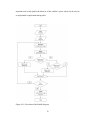
Figure 4.4.1: Flowchart of the Matlab Program ................................................................78
Figure 4.4.2: Flowchart of the Matlab Function ................................................................79
Figure 4.4.3: Output of the Matlab Program......................................................................79
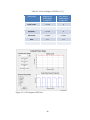
Figure 4.4.4: Layout of the Matlab GUI ...........................................................................81
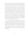
Figure 4.4.5: Payload 1 Output of the Matlab GUI ..........................................................82
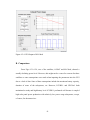
Figure 4.4.6: MISSat-1 Standard Power Mode GUI Output .............................................84
Figure 4.4.7: MISSat-1 Low Power Mode GUI Output ....................................................84
Table 4.5.1: Power Budget of ICUBE-1 ............................................................................87
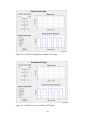
Figure 4.5.1: GUI Output of ICUBE-1 ..............................................................................87
Table 4.5.2: Power Budget of UPCSat-1 ...........................................................................88
Figure 4.5.2: GUI Output of UPCSat-1 .............................................................................88
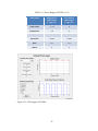
Table 4.5.3: Power Budget of AUSAT ..............................................................................89
Figure 4.5.3: GUI Output of AUSAT ................................................................................89
viii
Table 4.5.4: Power Budget of M-Cubed ............................................................................90
Figure 4.5.4: GUI Output of M-Cubed ..............................................................................91
ix
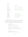
List of Abbreviations
ADCS ...............................................................Attitude Determination and Control System
ANSI ....................................................................... American National Standards Institute
AUSAT ............................................. Picosatellite of the University of Adelaide, Australia
BCR.............................................................................................. Battery Charge Regulator
BOL........................................................................................................... Beginning of Life
BRCLK ...................................................................................................... Baud Rate Clock
COM .................................................................................................... Communication port
COVE ............................................... CubeSat On-board processing Validation Experiment
CRRES ...................................................Combined Release and Radiation Effects Satellite
EPS................................................................................................. Electrical Power System
FET .....................................................................................................Flash Emulation Tool
GaAs/Ge ................................................................................ Gallium Arsenide Germanium
GUI ................................................................................................ Graphical User Interface
HDR ....................................................................................................High Dynamic Range
HESP .........................................................................................High Efficiency Solar Panel
I2C................................................................................................... Inter-Integrated Circuit
ICUBE-1 ................................. Picosatellite of the Institute of Space Technology, Pakistan
ISR ................................................................................................ Interrupt Service Routine
JPEG .............................................................................. Joint Photographic Experts Group
JTAG .............................................................................................. Joint Test Action Group
LED .................................................................................................... Light-emitting Diode
LEO ............................................................................................................. Low-Earth Orbit
mil ................................................................................................ one thousandth of an inch
M-Cubed ........................................................... Picosatellite of the University of Michigan
MISSat-1 ........................................................ Picosatellite of the University of Mississippi
MPPT .................................................................................. Maximum Power Point Tracker
RISC ............................................................................. Reduced Instruction Set Computing
RTOS ...................................................................................... Real Time Operating System
RX ............................................................................................................................. Receive
SPI ............................................................................................... Serial Peripheral Interface
TI .............................................................................................................. Texas Instruments
x
TX ........................................................................................................................... Transmit
UART ......................................................... Universal Asynchronous Receiver/Transmitter
UPCSat-1 ........................... Picosatellite of the Polytechnic University of Catalonia, Spain
USB ..................................................................................................... Universal Serial Bus
xi
1. Introduction
A CubeSat is a class of small satellites with short development time and low
production costs. It is designed for students of the undergraduate skill level. The satellite
is 1000 cm3 in size and less than 1.33 kg in weight. The Mississippi Imaging Space
Satellite is being designed as a CubeSat class satellite and will be launched as a
secondary payload. Its purpose is to capture terrestrial images. These images will be
transferred, while the satellite is in orbit, back to the University ground station. In order
to develop the CubeSat efficiently, the design was divided into its necessary subsystems
and each subsystem was then assigned to a project member. The subsystems presented
include the processor, payload, and power.
Figure 1.1.1: Small satellite in low earth orbit.
1
The primary mission of MISSat-1 is to capture images of earth and send those
images to the ground station at the University of Mississippi while in orbit. In addition,
the design and implementation provides an opportunity for students to practically apply
theoretical knowledge. The overall hope is that the project of designing and sending a
satellite into orbit can be continued in future years, building upon the knowledge obtained
from the realization of MISSat-1.
2
2. Processor Subsystem
I. Introduction
A. Project Description and Purpose
The processor subsystem is a central component with several responsibilities to
integrate all the elements of the satellite. Tasks include managing the power states,
driving communication with the ground station, initiating data collection, and
maintaining the system state. Within the processor subsystem is the actual
microcontroller, the motherboard along with integrated peripherals, and the operating
system.
Microcontrollers are self-contained systems that are often programmable for
interfacing with the outside world. Embedded systems make use of microcontrollers
designed to respond to environmental events by dedicating them to certain tasks such as
regulating room temperature. As microcontrollers have become more sophisticated, so
have the systems in which they are embedded. Microcontrollers with higher speed and
larger memory can even support what can be called an operating system that is driven top
down by user input and bottom up by environmental events.
3
Figure 2.1.1: A microcontroller in a quad flat package by Texas Instruments.
One of the main objectives of MISSat-1 is to capture terrestrial images. This
sensing application may employ microcontrollers to acquire data without making
physical contact with the subject or harsh environment under investigation. As
microcontrollers have become more complex their usage in remote sensing has increased.
At remote locations data is now able to be processed and compressed by microcontrollers
before it is sent back to the observer rather than being sent in bulk. With powerful
microcontrollers, a plethora of applications are made more available.
4
II. Subsystem Overview
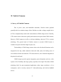
A. General Requirements
The components selected for the processor subsystem must meet certain unique
conditions to be suitable for space applications. A lightweight, low-power device that
does not sacrifice computing ability is what is needed for this particular project. With the
amount of CubeSat development projects increasing, there is a large number of space
proven microcontrollers from which to choose. Pumpkin, a CubeSat component provider,
has designed standardized motherboards that allow arbitrary microcontrollers to firmly
connect to peripherals.
Figure 2.2.1: A single board computer motherboard for harsh environments.
5
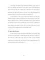
Many universities have chosen to use Pumpkin’s CubeSat Kit when developing
small satellites in an effort to simplify peripheral integration and troubleshooting. The kit
provides a standard set of connections that many devices made specifically for CubeSats
follow. Among the pluggable microcontrollers are products from Microchip, Silicon
Labs, and Texas Instruments that are used frequently in university focused projects.
Figure 2.2.2: This figure shows common CubeSat Kit Pluggable Processor Module for
Texas Instrument’s MSP430.
Each microprocessor has certain attributes that make it unique on the market;
however, the basic operation and capabilities from product to product are essentially the
same. Choosing a suitable microprocessor is based on the goal of the project. For
example, some products may lack in speed but triumph in durability. MISSat-1 needs a
microprocessor that is lightweight, power efficient, robust, and can handle a sophisticated
level of programming.
B. Hardware Selection
A space proven device is very important when considering what to select because
it suggests other groups chose it above other microcontrollers and demonstrates the
theoretical assumptions of performance may hold true. The Belgian OUFTI-1 CubeSat
6
project uses the TI MSP430 family of microcontrollers for their compatibility with
different styles of programming [1]. For MISSat-1, this flexibility proves useful
especially when considering MSP430’s ability to host a real time operating system that
will be discussed further in a later section.
The 11 gram TI MSP430F1612 uses between 1.8 V to 3.6 V and 200 µA in active
mode. It has a 16-bit RISC architecture with highly optimized instructions to reduce time
spent computing. The TI MSP430F1612 is equipped with built in operating modes such
as active mode and several levels of low power modes [2]. Depending on what state the
satellite is in (e.g. high activity or low activity) the software can switch among power
modes. Toggling through these modes with event driven interrupts is a key feature that
will allow the satellite to far exceed its power budget allowances. This device interfaces
with the rest of the subsystems through pins that lead to its many modules. The
MSP430F1612 has a 12-bit analog-to-digital converter, two modules for universal
synchronous/asynchronous receiver/transmitter use, and an inter-integrated circuit bus
that are needed to operate the antenna deployment, communications and camera boards,
and the electrical power system, respectively.
C. Software Selection
The style of operating system chosen to manage the hardware of the processor
subsystem is the real-time operating system (RTOS). A key characteristic of an RTOS is
its consistency in completing tasks. Salvo is such an operating system that is space
proven, supports the TI MSP430F1612, and is highly configurable with header files, user
7
hooks, and data types included that are written in ANSI C [3]. Salvo is small and efficient
allowing more data to be collected. It is also a multitasking RTOS that allows 16 levels of
priority for tasks that might be as simple as telling the communication system to send out
a beacon or as crucial as determining if there is enough power to capture an image. Of the
four supported compilers for the Salvo RTOS, the Rowley Associates: CrossWorks for
MSP430 has been chosen after gathering information from other satellite projects and
receiving quotes from each retailer. This particular compiler and IDE set is ideal based on
its low cost of $300 and a user license that is not limited on time.
Salvo is a multitasking real time operating system that is event-driven. The code
executes several tasks sequentially; however, the context is switched at a rate that makes
each task and corresponding event appear simultaneous. Programs written for Salvo do
not require the user to keep multitasking in mind as Salvo automatically handles services
such as task scheduling, access to shared resources, intertask communication, and
interrupt control [4].
8
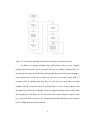
Figure 2.2.3: Real time operating system (Salvo) program execution flow chart.
In addition to running multiple tasks, Salvo allows tasks to have assigned
priorities that dictate the level of importance one has over another. Suppose there is a
low-priority task A that is periodically ran along with other tasks of the same importance
and a high-priority task B that is required to run every ten seconds. During task A’s
execution Salvo’s scheduler may stop task A to run task B to meet that ten second
deadline. After B’s execution context is switched back to A where it may continue from
the point from which it was suspended. Salvo also supports interrupt service routines that
may suspend any task. However, if a task must fully execute without a context switch
(e.g. a task that sends a packet to the communication board) interrupts may be disabled
prior to calling the non-reentrant function.
9
Figure 2.2.4: Context switching among tasks of varying priorities.
10
III. Development Configuration
A. Development Board Setup
The MSP430 Development Kit comes with a few items that allow the
microcontroller user to easily test and debug programs as well as work out some of the
issues associated with interfacing with peripherals. The kit includes the development
board, power supplies, USB wire, and a flash emulation tool. Defects from the
manufacturer could easily be the cause of issues early on in the development process.
This can be avoided by first powering on the development board with the +5 V standard
power supply and probing test points of interest. Below are the results of probing the test
points of the MISSat-1 development board after the proper jumpers were configured.
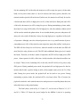
Table 2.3.1: CubeSat Kit development board’s expected and measured test point voltage
values.
Signal
Location
Value
Measured
+5V
TP9
+5V
+5.14V
VCC
TP12
+3.3V
+3.31V
VCC_MCU
TP20 TP44
+3.3V
+3.28V
VCC_232
TP21
+3.3V
+3.28V
V+_232
TP19
> +5V
+5.49V
V-_232
TP22
< -5V
-5.53V
+5V_SW
TP10
0V
0V
-RST/NMI
TP8 TP51
+3.3V
+3.30V
11
Each of the measured values was close enough to what was expected that
development moved forward. The next step involves installing drivers for the USB
connection between the PC and development board. This is not the main connection that
new programs will be loaded from; it is mainly used for I/O in conjunction with a service
such as HyperTerminal. With the drivers installed, the development board may be
powered on by simply connecting it via USB with or without a power supply. Test points
probed without a power supply for MISSat-1 were as follows.
Table 2.3.2: USB powered CubeSat Kit development board expected and measured test
point voltage values.
Signal
Location
Value
+5V Power Supply
+5V_USB
TP11
0V/+5V
0V
VCC_IO
TP13
0V/+3.3V
0V
A correctly operating MSP430 development board will have a starter
programming running each time it is powered on that features a blinking yellow LED.
Within this test program is a process that checks the ambient temperature of the
microcontroller. As there is no screen to view this result, a HyperTerminal or other
program such as TeraTerm must be set up to see the feedback from the running code.
12
B. PC Connection
Programs running on microprocessors may have the functionality of displaying
useful information to the user on a monitor and connection software. Regularly gathered
information or even input from the user may be exchanged via such a program. For
MISSat-1 the computer communication software chosen for initial use is HyperTerminal.
The settings that proved successful were as follows.
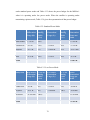
Table 2.3.3: HyperTerminal settings for default MSP430 program display.
Bits per Second
Data Bits
Parity
Stop Bits
Flow Control
9600
8
None
1
None
These parameters indicate that the baud rate is 96000 with eight data bits in each
character. There is no parity used for error detection, but each block of data is specified to
be complete with just one bit after the 8 bits of information. Upon successful
configuration of the PC, the starter programming produces an output similar to what is
shown below.
13
Figure 2.3.1: Default program output viewed in HyperTerminal.
With everything working properly the test program uses the HyperTerminal to
display the ambient temperature that it has measured repeatedly at a short interval. At this
point the development board, power supply, and PC connection are verified to be
working properly. The next step is installing an integrated development environment to
write and debug new programs created to meet the goals of the satellite mission.
14
C. Integrated Development Environment
The integrated or interactive development environment allows programmers to
write, test, and debug software. The environment used in this project is CrossWork’s
CrossStudio for MSP430. This product provides the usual compiler, macro assembler,
linker/locator, and Salvo libraries; however, what makes it unique is its core simulator
and JTAG debugger. The core simulator allows programs to be uploaded to a virtual
microcontroller for general testing rather than having all the physical equipment that may
not be needed for troubleshooting a certain part of the program. This feature is useful in
that it prevents time from being wasted dragging out the components and perhaps being
damaged from movement or foreign objects. The JTAG debugger has proven essential
because it allows the software developer run the program line by line on the
microcontroller.
Initially CrossStudio would not identify the CubeSat Kit development board as a
recognized device so a bit of troubleshooting took place to correct the issue and report the
solution on various forums. To connect to a PC for use with CrossStudio, a supported
flash emulation tool, MSP-FET430UIF, is used.
15
Figure 2.3.2: TI MSP430 Flash Emulation Tool for PC connections.
From there it is expected that navigating to the “Target” menu and selecting
which method of connectivity to use will prepare the device for programming, but there
is a flaw in how Texas Instruments has moved forward with firmware upgrades to their
devices. CrossStudio initially displays the error message “Can’t connect to target USB:
Could not find MSP-FET430UIF on specified COM port” which misleads the user into
thinking the incorrect COM port has been assigned. Under further investigation it was
determined that this development environment only communicates with the latest
firmware known at the time of installation. Rather than installing a previous version the
firmware of the flash emulation tool needed to be updated.
Texas Instruments endorses an open source command line programmer called
MSP430 Flasher. It is downloaded and run as an executable that identifies connected
16
Texas Instruments devices via the flash emulation tool. During runtime, the flasher
detects conflicts and prompts the user to choose a course of action.
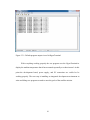
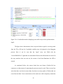
Figure 2.3.3: MSP430 Flasher Command Line Programmer Interface.
If an outdated version of firmware is detected the flasher recommends updating
by entering “Y” as a confirmation. The software then updates the firmware without any
further assistance. The command line programmer can be useful in other ways as well. If
there is a voltage outside the desired range when using the flash emulation tool along
with the development board and PC a security fuse may be blown. This fuse can be reset
with this executable as well. Another great option supported by the command line
17
programmer is the ability to load programs, read memory, and verify memory without the
use of a development environment.
With the firmware updated and drivers installed, custom programs are ready to be
built and run on the microcontroller. The properties in CrossStudio may vary from user to
user. The settings that resulted in successful communication after connecting the
development board can be seen in the figure below.
Figure 2.3.4: Flash Emulation Tool connection properties for CrossStudio.
18
IV. Peripheral Integration
A. Serial Communication
Microcontrollers are able to control peripherals by the use of pins that send and
receive signals among devices. This communication can be as simple as raising the
voltage on one pin as another pin observes a voltage decrease; however, many standards
have been established for efficiency. Serial communication protocols such as UART,
I2C, and SPI are quite common, and many microcontrollers support multiple standards
[5].
UART communication is seen often with CubeSat components because of its
reconfigurable and asynchronous nature. From a physical standpoint, UART systems
have four wires; ground reference, 3.3V/5V high reference, transmit line, and receive line
[6]. When these four wires are connecting the two communicating devices, there is a
common high and low reference. Two separate receiving and transmitting lines allow the
devices to transfer information simultaneously as each store the data into buffers until it
is needed.
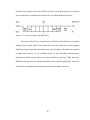
Data sent via a UART connection follows a general character framing scheme but
can be altered by adjusting control registers in the controlling microprocessor. The
19
character frame begins with a start bit followed by the actual data being sent. A parity bit
for error detection is optional and is followed by a specified number of stop bits.
Figure 2.4.1: UART character framing scheme.
The rate at which devices communicate is referred to as the baud rate, or symbols
transferred per second. Both devices must have the same baud rate to work together
which may also be specified via microprocessor control registers. The baud rate is limited
in speed and accuracy by the available clocks of the controlling microprocessor.
Programmers divide system clocks of a microcontroller to generate UART baud rate.
Different baud rates may be selected depending on the particular application. Some uses
call for faster communication, but higher baud rates have higher error rates.
20
Table 2.4.1: Commonly used baud rates, settings, and errors [7].
The table above demonstrates how certain baud rate clocks (BRCLK) of the
MSP430 family may be divided to obtain desired baud rates. This information is provided
by Texas Instruments to help users choose baud rates wisely. It can be seen that for a
specific clock the baud rate is a factor for the error percentage.
B. Payload
The payload for MISSat-1 consists of terrestrial images captured by an onboard
camera. It is important that this device is understood so that commands and data can be
efficiently passed to and from the camera. A JPEG Module handles the compression of
images captured by the camera and hosts a serial interface featuring a UART core.
21
Figure 2.4.2: On board camera pin layout.
The figure above shows the pins available for interfacing the camera board.
Because this camera is widely used and not just for CubeSat projects, it does not feature
CubeSat Kit bus connectors for simplified interfacing. The four wires of the camera’s
UART connection are instead directed to where they can connect to the microprocessor’s
UART module via a protoboard.
22
Figure 2.4.3: Protoboard that converts arbitrary devices to use the CubeSat Kit bus
connector scheme.
It is important to rout these wires to pins that lead to one of the UART modules
designated for general use. Example code from Salvo designates that the communication
board should use UART module 1 while other peripherals may use UART module 0. The
pins for UART 0 are specified on the CubeSat Kit motherboard datasheet.
The camera board initiates communication by listening for a synchronization
signal. Those working on the camera subsystem have developed a program that sends this
signal to the camera board until a confirmation signal is received or a set number of
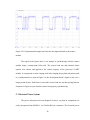
attempts have been reached for timeout purposes. The synchronization signal in the
figure below is sent from a laptop to the camera. The signal is five bytes long, and a
positive confirmation was received from the camera in return.
23
Figure 2.4.4: Synchronization signal sent from a laptop and correctly received by the
camera board.
The first step for the processor subsystem to control the camera module is
ensuring that the transmitted signals are understood by each device. If the processor can
receive a confirmation from the camera after sending the synchronization signal then a
positive handshake has occurred. This means the two devices are using the same
character framing scheme and baud rate. All other commands to and from the camera will
be understood once effective communication is established.
To ensure the processor has the ability to send and receive arbitrary signals a
quick test was conducted. In this setup the transmitting pin of the UART module is
directly connected to the same module’s receiving pin. With the CrossStudio
development environment in debug mode the received information can be seen through
the IDE’s ability to view registers and buffers in real time.
24
Figure 2.4.5: Block diagram to check sending and receiving signals with the
Development board.
The block diagram of Figure 4.5 helps to visualize the way this particular test is
wired. The synchronization signal is sent using CubeSat Kit Salvo commands and the
incoming characters are received into an array. The user may toggle whether or not the
wire between the UART TX and RX pins are connected. Receipt of expected signals is
indicated with an onboard LED. Successful operation results in the LED being on when
the pins are connected and off otherwise. The task code written for this may be found in
the appendix section.
25
Figure 2.4.6: CrossStudio interface displaying successful receipt of the synchronization
signal.
The figure above demonstrates what is expected when a signal is correctly passed
from the TX to RX pin. In CrossStudio variables may be displayed in the debugging
process. Here it can be seen that the “input” array was filled with the
“0xAA01B00005AA” signal that was transmitted. Because the information now stored in
the array matches what was sent out, the section of code that illuminates the LED is
entered.
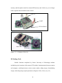
As mentioned before, the camera board does not feature CubeSat Kit bus
connectors so other means of connecting the processor must be used. There are just four
wires that these two devices must share, but there are many points of failure that can
occur between them. Loose connections are the main issue with a temporary connection
26
such as this. A solderless breadboard is used to hold the reference for ground and +5V.
As camera control is further developed an established work station with probing points
for a multimeter and oscilloscope has been made.
Figure 2.4.7: Camera interfacing work station.
At all times the developer can read the UART reference voltage (e.g. +5.06V is
the reference here) and using the Analog Discovery USB oscilloscope the sent signals are
viewed. No switching connections or change in probe locations is needed with such an
extensive work station.
27
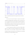
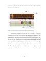
Figure 2.4.8: Synchronization signal sent from the development board to the camera
module.
The signal in the figure above is an attempt at synchronizing with the camera
module using a custom-made Salvo task. The correct baud rate and character frame
options were chosen and applied to the control registers of the processor’s UART
module. In comparison to what a laptop used in developing the payload subsystem sends
as a synchronization as seen in Figure 4.4, the development board’s signal is sent over a
longer period of time. Each frame is sent at the correct baud rate, but the spacing between
characters in Figure 4.8 prevents the camera from properly synchronizing.
C. Electrical Power System
The power subsystem has been designed in such a way that its components are
easily incorporated into MISSat-1 via CubeSat Kit bus connectors. The electrical power
28
system board is stacked along with other peripherals to fit neatly within the allowable
dimensions of the CubeSat [8].
Figure 2.4.9: Electrical power system CubeSat Kit bus connection pins.
Communication between the processor and EPS is driven by an I2C bus. No
adjustments have to be made to the CubeSat Kit bus connector because there are no other
peripherals in this project that use the serial data line and serial clock line of the I2C bus.
The only issue with using this specific EPS board is that the microcontroller within the
device operates on data differently than the processor subsystem microcontroller. The
difference is the order of storing bytes of a data word in either big or little endianness.
The EPS is big endian while the microcontroller of the processor subsystem is little
endian.
29
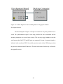
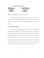
Figure 2.4.10: Data stored in Big versus Little Endianness.
The term “endian” is an allusion to a great war in Gulliver’s Travels, but the issue
is resolved with simple conversion code. Beyond the data transfer between the EPS board
and processor subsystem is the use of the real time operating system to manage power in
a safe way.
D. Communication Board
The radio has the responsibility of communicating with the ground station while
the satellite is in orbit. Information such as subsystem statuses must be collected during
flight and continue to be transmitted throughout the life of MISSat-1. The communication
board chosen for MISSat-1 is of the AstroDev Helium Radio product line and adheres to
the CubeSat Kit standards on size and bus connection [9]. Like the payload, the
communication board will make use of one of the UART modules of the processor to
send and receive data. Unlike the EPS board, this radio is built around the same
microcontroller as the processor subsystem so no endianness issues will be found.
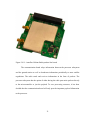
30
Figure 2.4.11: AstroDev Helium Radio product line board.
The communication board relays information between the processor subsystem
and the ground station as well as broadcasts information periodically to meet satellite
regulations. The radio sends and receives information in the form of packets. The
processor subsystem has the option of either having the radio pass entire packets directly
to the microcontroller or just the payload. To save processing resources, it has been
decided that the communication board will only pass the important payload information
to the processor.
31
Figure 2.4.12: Packet structure for commands and data (top) and packet header
description (bottom).
With this decision in place, the radio will take on a portion of the responsibilities
associated with processing incoming and outgoing data. All information exchanged
between MISSat-1 and the ground station will be in the AX.25 link-layer protocol
specification because of its widespread use in the small satellite community.
32
V. Conclusion
The goal of this section has been to lay the initial foundation for further
development of MISSat-1 as it pertains to the microcontroller that directs all of the
satellite’s functionality. Both hardware and software considerations have been
documented as well as the reasons for specific product selection. Using this paper as a
guide, groups may begin to develop their own processor subsystems without repeating
some of the troubleshooting issues explored during this project. Programs used regarding
MISSat-1’s operating system are available through purchasing Pumpkin’s Salvo RTOS.
33
3. Payload Subsystem
I. Introduction
A. Project Description and Purpose
Communication between the camera microcontroller and the satellite processor
will be explored, with the goal of successful commands sent and received from the
processor. Communication attempts in the past between camera and processor
development board have been unsuccessful. Upon successful communication with the
processor via the UART interface, functionality designed by recent University of
Mississippi graduates will be implemented with the processor.
In previous years students have designed a GUI to interface and experiment with
camera functions and settings through a computer. The final configuration must take the
camera functionality and camera-computer interactions developed by past students and
implement it with the processor. Additional functionality was added such as are obtaining
storage and file information, luminance, and deleting files on the camera. Resolution and
compression ratio must be able to be adjusted to ensure that the images will be able to be
transmitted when the satellite passes over the ground station. The satellite will have a 10
34
minute window to transmit images while in low earth orbit. Testing will also be
conducted to determine the best initial capture settings of the camera before being
launched into space. Images were captured to test the effects of various lighting and
distances.
Prior work on the camera payload included selection of the camera and
programming of an interface that communicates directly with the camera microcontroller
from the user’s computer. The C6820 Enhanced JPEG Module manufactured by
COMedia was selected as the camera subsystem based on weight, size, image
compression, and power usage considerations. Additionally, an interface was
programmed in C# to communicate with the camera board directly from the user’s
computer through a serial connection.
B. Background Information
Often times CubeSats choose a camera as their primary payload system. Camera
payloads can be used for weather forecasting, space imagining, and surveillance systems.
These images are usually low resolution due to the mass, power, and bandwidth
constraints of CubeSats [10].
In previous years, University of Mississippi students designed a GUI to interface
and experiment with camera functions and settings through a personal computer. The
final configuration must take all of the camera functionality and computer interactions
developed and implement it with the CubeSat processor. Additional functionality was
added such as obtaining storage and file information, observing luminance, and deleting
35
files on the camera. The old code was also modified to ensure proper exception handling
and bugs presented were fixed. Functions to adjust image resolution and compression
ratio were implemented to ensure that the images will be able to be transmitted when the
satellite passes over the ground station, as the satellite will only have a 10 minute window
per orbit to transmit images while in low earth orbit.
Smaller images were taken to ensure that images can be successfully transmitted
in the window. Testing was conducted to determine the best initial capture settings of the
camera before being launched into space. Special considerations for space imaging
(lighting conditions in space, camera orbital speed, etc.) were researched and taken into
account in the programming of the camera subsystem. Images were captured to test the
effects of various lighting and distances.
36
II. CubeSat Cameras
A. Survey of CubeSat Cameras
Due to power, mass, and bandwidth constraints, CubeSat camera payloads
generally take low resolution images. Most CubeSats use either a charge coupled device
(CCD) or complementary metal oxide semiconductor (CMOS) image sensor. Generally,
CCD cameras retrieve data more quickly and consume more power than CMOS cameras.
However, CMOS cameras are still an evolving technology, whereas CCD is a mature
technology. The general trend of CubeSat cameras is towards CMOS because it
consumes less power and lasts longer in space [10].
The durability of CMOS image sensors is due to the fact that all functions can be
integrated in the chip, which minimizes leads and solder joints; the leading cause of
circuit failure in harsh environments. CCD sensors however, have functions integrated on
the printed circuit board.
CMOS imagers provide superior integration, power dissipation, and size, at the
expense of low flexibility and image quality, especially in low light. This makes CMOS
technology ideal for space-constrained applications where image resolution is of no
consequence, such as security cameras, PC videoconferencing, and wireless handheld
devices.
37
CCD imagers offer higher image resolution and flexibility, at the expense of
device size. Flexibility means that the user can achieve greater system differentiation
with a CCD sensor than with a CMOS sensor. This makes CCD sensors ideal for
applications where high quality images are necessary, such as digital photography and
broadcast television. The cost of these two sensors are comparable [11].
For our CubeSat, we chose to use a CMOS sensor due to our size and power
constraints, the details of which will be discussed in the following sections. In the “Space
Imaging Conditions” section, we determine the luminance of space to better understand
the conditions our camera will be performing under. This is necessary to determine the
proper settings to take pictures in space, and to see if the CMOS sensor has poor
resolution in different lighting situations, as mentioned previously.
B. Camera Specifications
We have chosen to use the C6820 Enhanced JPEG Module in our CubeSat, which
was also used as payload in the F-1 CubeSat designed at FPT University in Vietnam [12].
The C6820 has a CMOS image sensor and has the ability to adjust resolution,
compression ratio and many other values necessary for space imaging applications. The
camera specifications can be found in Figure 3.2.1.
38
Figure 3.2.1: C6820 Module Specifications [13]
Figure 3.2.2: C6820 Dimensions (In Centimeters) [13]
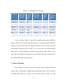
Table 3.2: C6820 Power Consumption
Voltage Draw
5.27 V
5V Input
Current Draw
.245 A
Capture Mode
.235A
Download Mode
.187A
Idle Mode
Figure 3.2.3: C6820 power measurements [13]
39
III. Previous Work
A. Camera Selection
The weight restriction for CubeSats is 1.33 kg for the entire satellite. The frame of
the satellite takes up a third of the allotted weight, so the camera must weigh less than
10g to ensure there is enough weight leftover for the components of the other subsystems.
The volume of the entire CubeSat is restricted to a 10cm x 10cm x 10cm cube. The
camera should occupy less than 1cm3 to ensure there is room for larger components, such
as batteries and processors.
The entire satellite runs at a very low power and must be able to recharge itself
with solar panels attached to the sides of the satellite. At full charge, the batteries hold
about 10Wh, so an ideal camera would use less than 1W of power. The camera uses the
most power while capturing an image, and uses nearly no power in while it is in idle
mode.
The C6820 Enhanced JPEG Module, manufactured by COMedia, was chosen
because it met all weight and size requirements of MISSat-1 and can be easily integrated
into the satellite. An image of the C6820 can be found below in Figure 3.2.3. Integration
of the C6820 is simpler because it comes with an evaluation kit. The evaluation kit
complies with the MISSat-1 size constraints and includes an on-board JPEG compressor,
on-board
40
memory, and the option to attach an external SD memory card. In this way, we no longer
need a separate microcontroller for the camera.
DC/TV
UART
SD Card Socket
Mini USB
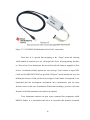
Power On
Figure 3.3.1: COMedia C6820 [14]
B. Existing Code
Notable functions completed by former University of Mississippi students
included on prior iterations of the camera GUI include: Synchronization between camera
and computer, switching between various camera modes, taking images, downloading
images, and setting image capture parameters (Exposure Value, Color, etc.) [15].
41
The camera synchronization function is used to open the communication port on
the computer and send the proper synchronization signal to activate the camera. The
function repeatedly sends this signal until the camera responds with the proper
hexadecimal values to indicate the camera has been synchronized or until the function
times out.
The “change camera modes” function has also been implemented in past years.
The camera has three modes: idle, capture, and playback. The latter mode will not be
used on the MISSat-1, as it is only for video recordings. The idle mode allows users to
manipulate images currently stored on the camera, while the capture mode allows images
to be taken. In idle mode, the camera’s capture parameters can be adjusted, such as the
exposure value and color properties.
The download image function operates by sending the camera a series of bytes
indicating a download request and the file to be downloaded. The camera replies with a
series of bytes that specify the image’s file size, the number of packets the image has
been broken down to, and the filename. The camera GUI uses this information to loop
through the packets being sent to process the image and store it as a JPEG file.
The following section details the improvements added to the previous version of
the camera GUI.
42
IV. Programming the Camera Interface
A. Camera Operation
The camera GUI operates by sending bytes of information to the camera
microcontroller and waiting for response. Typically, the sent code from the GUI to the
camera is an array of five hexadecimal bytes, bookended by the bytes “0xAA.” The GUI
then waits for an array of hexadecimal bytes from the camera. This received array usually
consists of six hexadecimal bytes, bookended by the bytes “0xAA.” This returned array
contains valuable information as to the success or failure of the operation. For more
complex functions such as downloading an image or synchronization with the camera, a
series of arrays may be returned, all of which contain information regarding the status of
the camera. One major improvement of the camera GUI discussed in the next section is
the analysis of the received byte array in order to ensure the stability of the GUI and
exception handling.
B. Improvements and Modifications
The window to download images from the satellite is approximately 10 minutes
every day. Thus, communication with the satellite can be quite cumbersome and proper
file management is needed to ensure that all processes are executed efficiently during the
10 minute window. The following functions were added to the existing camera GUI to
43
ensure that there would be no confusion when attempting to access camera files. Each of
these functions rely on low-level exception handling to ensure the program does not
crash.
Delete Function
The delete command deletes files directly from the camera memory. However,
there is no way to directly observe the contents of the camera memory. As a result,
testing of the delete function is limited to taking a picture, downloading the picture,
deleting the picture, then verifying that the deleted picture cannot be downloaded again,
or, taking a picture, deleting the picture, taking a new picture, and verifying that the old
picture filename now holds the new picture. The delete function makes use of the ID and
Parameter commands of the camera. Testing of the delete function revealed various bugs
in the camera GUI. Attempts to download nonexistent pictures resulted in an
“IndexOutOfBounds” exception. Handling of these exceptions is done through low level
checking of bytes returned from the camera microcontroller, instead of higher level
exception handling such as try-catch blocks. This and other modifications to the code are
discussed in later sections.
Memory Management
In order to allow for greater user control over file management and downloading
of images, additional functionality was added to the GUI to work in conjunction with the
delete function.
A memory function was implemented to display the memory available on the
camera in megabytes, the number of files on the camera and the number of images that
can be taken given the current settings. Testing of the function consisted of running the
function to observe the current memory state, deleting a file, and running the function a
44
second time to confirm that the total number of files has decreased by one, and that the
available memory has increased. This also verifies the functionality of the Delete
function implemented last week. Because the memory information is obtained by sending
a sequence of bytes to the camera microcontroller, the memory update function cannot
update in real-time. Instead, a button must be pressed to refresh the memory data.
Low-Level Exception Handling
Many of the camera functions on the existing GUI had no exception-handling.
These functions were updated to take advantage of the return bytes from the camera to
better understand the camera processes. These function now interpret the return bytes and
can stop the program from crashing if a function is not successful. Most notably, the
download function implemented in past years can now operate fully without crashing.
The prior version of the download function would crash the program if an error occurred,
or if the file could not be found. With low-level exception handling, this can be avoided.
Resolution and Compression Ratio
A resolution and compression ratio setting was implemented in order to manage
the size of the images taken. Because there is a short window of opportunity to transmit
images from the satellite to the ground station, achieving an appropriate image size is
imperative. The MISSat-1 can take pictures in 1280x960 and 640x480 resolution and a
compression ratio between 1 and 45. Many universities choose to take images with
640x480 resolution. The COMPASS-1 FH Aachen University in Germany used a very
similar camera as the MISSat-1 and only takes pictures in the lowest resolution to
improve transmission time. Testing of the compression ratio and resolution setting shows
that the addition of these operations allow the user to significantly decrease the size of the
45
image to be downloaded. Assuming a 640x480 pixel RGB image will be taken, with three
bytes per pixel, the image size can be calculated as follows:
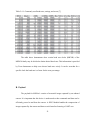
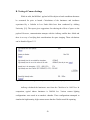
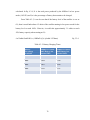
The transmission rates available are: 9600 baud/s, 4800 baud/s, 2400 baud/s, and
1200 baud/s. The amount of time needed to transmit an image at each of the transmission
rates are given in Figure 3.4.1.
Transmission Times
TX Time (1 image)
Sec
768
9600 baud/s
1536
4800 baud/s
3072
2400 baud/s
1200
1200 baud/s
Figure 3.4.1: Table of transmission times. [15]
TX Rate
Min
12.8
25.6
51.2
102.4
Optimistically, the satellite pass over time will be around ten minutes. From the
Figure 3.4.1, it is evident that even the fastest transmission rate cannot transmit an image
without compression. Assuming a transmission rate of 2400 baud/s, a pass time of eight
minutes, and a file size of 921,600 bytes (calculated above), a compression ratio of 1.4:1
is needed. Further testing must be conducted to determine the optimum compression ratio
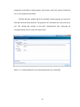
for implementation. An image of the GUI can be found in Appendix II.
46
V. Integration of Camera Interface into MISSat-1
A. Space Imaging Conditions
While in space, MISSat-1 will be subject to extremely harsh lighting conditions.
These conditions need to be accounted for and simulated to ensure quality images of the
Earth are taken. Many of the resources for taking pictures of space are written by
astrophotographers, who primarily take pictures of Earth from the International Space
Station. While this information is helpful in understanding the imaging conditions of
space, the cameras used for these applications are very high quality DSLR cameras with
highly tunable exposure and aperture values. In order to understand how space affects
CMOS image sensors, further investigation is needed.
CubeSats with similar camera payloads have been launched by the University of
Michigan and VIT University in India. These two universities provide extensive
documentation of their camera testing and settings. Both universities believe that it is
important to test the functionality of the camera in the extreme cold temperatures and
radiation of space. Additionally, both universities believe it is important to protect the
camera lens from exposure to the sun.
The University of Michigan CubeSat uses a CMOS camera and a compression ratio
of about 10 [16]. They tested their camera settings by simulating Earth’s luminosity in
47
lab, taking pictures of modulation transfer function test charts, and testing the necessary
exposure time for blur free photos.
VIT University’s VITSAT-1 also uses a CMOS camera manufactured by
OmniVision. They cite the following as difficulties that arise when attempting to take
pictures in space: high power density of sunlight, low temperature of space, high
radiation intensities, directional stability, power consumption, and weight of the camera
[17]. Because CubeSats have a short pass time, low resolution images must be taken to
ensure the image can be transmitted in a reasonable amount of time. CubeSat cameras
also require adjustable exposure settings. Because most camera modules are designed to
be used for terrestrial applications such as mobile phones and webcams, an adjustable
exposure is needed to ensure the camera can take quality images of the Earth under the
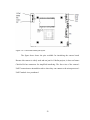
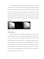
harsh luminance conditions of space. Figure 3.5.1 shows images taken in space using the
same camera module as the VITSAT-1, taken by a University of Tokyo CubeSat at the
Intelligent Space Systems Laboratory.
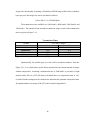
Figure 3.5.1: Intelligent Space Systems Laboratory, University of Tokyo
To illustrate the importance of adjustable camera settings for space imaging,
Figure 3.5.2 contains images taken from a similar OmniVision CMOS camera taken by
COMPASS-1 of FH Aachen University of Applied Sciences in Germany. COMPASS-1
uses a camera module with an automatic exposure setting [18]. Because of the strong
48
illumination in space, the automatic exposure cannot adjust to a proper setting to take
proper images of Earth. The COMPASS-1 also has a neutral density filter installed.
Neutral density filters are used to reduce all wavelengths of light equally. In doing so, a
longer exposure time can be used, without oversaturating the images. The use of the filter
provided satisfactory images on Earth, but failed when implemented in space. Despite the
use of a filter, the images are still incredibly saturated, which speaks to the importance of
properly testing camera settings on Earth.
Figure 3.5.2: Images taken by the COMPASS-1 CubeSat. The satellite antenna and the
contour of the Earth can be seen in some of the images.
The MISSat-1 camera has an adjustable exposure value with range -2 to 2. The
camera settings and the testing of the camera is detailed in the following section.
49
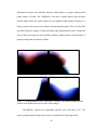
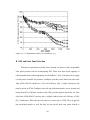
B. Testing of Camera Settings
While in orbit, the MISSat-1 payload will be subject to harsh conditions that must
be accounted for prior to launch. Calculations of the luminance and irradiance
experienced by a CubeSat in Low Earth Orbit have been conducted by Aalborg
University [19]. The report gives suggestions for reducing the effects of space on the
payload. However, communication attempts with the Aalborg satellite have failed and
there is no way of verifying their considerations for space imaging. These calculations
can be found in Figure 3.5.3.
Figure 3.5.3: Calculated light intensity values seen by CubeSats [19].
Aalborg calculated the luminance seen from the CubeSat to be 16425 lux. In
comparison, typical indoor luminance is 200-500 lux. Various camera lighting
configurations were tested in an anechoic chamber. These configurations attempted to
simulate the high intensity, high contrast scenes that the CubeSat would be capturing.
50
C. Image Processing
In order to improve the quality of images taken in space, various image
processing techniques were explored. Two filtering techniques were considered:
Laplacian Filtering and Highboost Filtering. Both Laplacian and Highboost filtering are
spatial filtering techniques.
Laplacian Filtering
Laplacian filtering is a spatial filtering technique to sharpen images by creating a
filter mask based on the discrete formulation of the Laplacian operator. The discrete
formulation of the Laplacian for a function of two variables is:
Where the second order derivative in the x-direction and y-direction is:
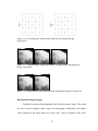
The filter mask constructed from these equations is given in Figure 3.5.4.
0
1
0
1
-4
1
0
1
0
Figure 3.5.4: Laplacian filter mask used for image sharpening.
51
The corresponding filter mask gives the second-order derivative in the horizontal
and vertical directions. The convolution of the filter mask with the original image yields
the edges of the original image. The edges can be added to the original image to yield a
sharpened version of the original image. It is important to note that the above filter mask
considers only the horizontal and vertical changes in an image. To account for diagonal
changes in intensity, the center value of the mask is replaced by -8 and the four terms that
are currently set to 0 are replaced by 1 [20]. The results of Laplacian filtering can be seen
in Figure 3.5.5.
Figure 3.5.5: Original image, Laplacian mask, and sharpened image
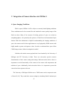
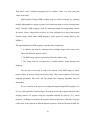
Highboost Filtering
Highboost filtering is a spatial filtering technique where the filter mask is
obtained by subtracting a blurred version of the image from the original image. The mask
is then scaled by a constant factor and added to the original image. Figure 3.5.6 shows
two different kernels used to blur the image. The averaging filter blurs the image by
setting pixel values to the average intensity of its surrounding neighbors. The Gaussian
filter blurs images in a similar manner, but weights the pixels differently based on a
Gaussian distribution. The coefficients are necessary to preserve the overall image
intensity. The effects of the averaging mask can be seen in Figure 3.5.7 and the effects of
the Gaussian mask can be seen in Figure 3.5.8.
52
Figure 3.5.6: Averaging and Gaussian filter mask used for image blurring,
respectively.
Figure 3.5.7: Original image, image blurred with averaging mask, and sharpened
image, respectively.
Figure 3.5.8: Image blurred with Gaussian mask, and sharpened image, respectively
High Dynamic Range Imaging
Traditional cameras take photographs with a limited exposure range. This results
in a loss of detail in bright or dark sections of a photograph. Additionally, the radiance
values captured by the image sensor are not the “true” values of radiance of the scene.
53
Thus, there exists a nonlinear mapping between radiance values in a scene and pixel
values in an image.
High Dynamic Range (HDR) imaging improves detail in images by capturing
multiple photographs at varying exposure levels and merge them to create a broader tonal
range. Typically, HDR imaging is used for enhancing images and exaggerating contrast
for artistic effects. Images taken in space are often subjugated to a larger than normal
dynamic range, which makes HDR imaging a viable option for images taken by the
MISSat-1.
The implementation of HDR imaging is split into three components:
1. A radiance map must be constructed from multiple images of the same scene
taken with different exposure values.
2. The HDR image must be reconstructed from the radiance map.
3. The image must be converted into a suitable display image through tone
mapping.
The last step is necessary to reduce the contrast of the HDR image to ensure
proper display on devices with lower dynamic range. There exists a number of local tone
mapping procedures that exist, and the proper tone mapping algorithm must be
determined.
We are currently in the process of testing and implementing HDR imaging to see
if it is a viable option for CubeSat images. In order to recover the response function of the
imaging process, we propose using the algorithm outlined by Debevec [21], which
proposes a technique to construct the response function based on a collection of images
of the same scene captured at different known exposures. With the function in hand, the
54
pixel values of the pictures with varying exposures can be used to construct a radiance
map, which covers the entire dynamic range of the scene.
Response Function Recovery
When a digital image is taken, the exposure X is given as the product of E, the
irradiance of the film and Δt, the exposure time. After digitizing and processing, the
exposure X becomes a new number, Z, a nonlinear mapping of the exposure at each pixel.
This transformation is the characteristic curve of the film and encompasses the
irregularities introduced by processing the image. The above can be expressed as such:
This equation can be rewritten as:
where i is the pixel index and j is image exposure index. In this equation, Ei and Δt are
known and the function g and Zij are the desired values. Debevec includes a smoothing
factor and a weighting term to more accurately fit the data, and solves the overdetermined
system [21]. With a recovered g, the pixel values can be converted to the appropriate
radiance values with given Δt for any image taken. Figure 3.5.9 shows the process of
constructing the mapping between exposure and pixel value given three images.
Debevec’s code can be found in Appendix III.
55
Figure 3.5.9: Pixel value plotted as a function of log exposure given three images [22].
56
VI. Conclusion
A. Future Work
After successful construction of the radiance map of a series of images, tone
mapping must be performed in order to properly display the HDR image. There are a
variety of tone mapping techniques that exist, the simplest of which consists of applying
a global transfer curve. However, when the image has an unusually high exposure range,
global tone mapping techniques fail to preserve exposure details. Instead, local tone
mapping is needed. Durand [23] details a local tone mapping technique to display HDR
images while preserving edge details. The process works by decomposing the HDR
image into a base layer and a detail layer. The base layer has contrast reduced, thus
preserving details in the displayed image. A bilateral filter is used to obtain the detail
layer due to its edge-preserving properties.
Because HDR images use multiple images of the same scene with different
exposures, it is imperative that the camera remain relatively steady during the imaging
process. A camera function should be implemented that iterates through a series of
exposure values and takes images automatically at each of them, as manually taking and
adjusting exposure values is too timely to produce quality images for HDR imaging.
Additionally, further testing of the behavior of the CubeSat in space conditions
must be conducted. The possibility of a neutral density filter and other mechanical
57
techniques to improve imaging should be explored. Currently, the camera has a “measure
luminance” function, which should be implemented to provide insight on image scenes.
Further investigation must be conducted to determine the best configuration to simulate
space conditions on Earth.
58
4. Power Subsystem
I. Introduction
A. Project Description and Purpose
Of the subsystems of the MISSat-1, the power subsystem will be the main focus
of the last few sections of this paper. The power subsystem is responsible for managing
the power for the entire satellite. The main function of the power subsystem is to collect,
store and distribute power. Once launched, if the satellite is in the sun, power for the
satellite is collected through the solar panels surrounding the exterior of the CubeSat
which is then transferred to the battery and the other subsystems that require it. When the
satellite is in the dark, the battery will transfer power to the subsystems that require it.
Therefore, the power subsystem that is selected for the MISSat-1 must be able to
integrate seamlessly with the other subsystems of the satellite.
59
II. Solar Panels
A. Solar Cell Degradation
One of the initial responsibilities of the power subsystem is the selection of both
an electrical power system (EPS) and solar panels that will be best suited for the MISSat1. With regards to solar panels, in order to make a well-informed decision, it is essential
to first become familiar with not only how solar panels function but how they are affected
by a space environment. A space environment is known to negatively impact the lifespan
of a satellite and, in most cases, the typical lifespan of a CubeSat only ranges from 3 to 9
months. Maximizing the lifetime of the CubeSat would be a great advantage since it
would allow the satellite a longer time period in which to collect data. Therefore, some
time was spent investigating the main causes of solar cell degradation. This topic is of
particular interest for the MISSat-1 because it not only influences the overall lifespan of
the satellite but the power intake as well. On this topic, a term to be familiar with is
beginning of life (BOL). BOL power for a solar panel refers to the amount of power the
panel can take in before it has been exposed to a space environment, at the start of a
satellite’s mission [24]. Another important term is solar cell efficiency, which simply
refers to how much solar power can be converted to power for the satellite.
After looking into the issue, it was found that solar cells can be degraded in space
due to three main reasons: exposure to atomic oxygen, thermal cycling and ultraviolet
60
radiation. Atomic oxygen itself is a result of bursts of ultraviolet radiation that cause the
breakdown of molecular oxygen. According to the European Space Agency, the
concentration of atomic oxygen in space is dependent upon both the satellite’s altitude
and the current solar activity that the satellite is exposed to [25]. Atomic oxygen is
notably a concern for satellites in low earth orbit (LEO), which is where the MISSat-1
will be orbiting. Prolonged exposure negatively impacts the satellite by eroding the
satellite’s surfaces including the solar cells. Eroded solar cells result in drastically
reduced solar cell efficiencies. However, the susceptibility of solar cells to atomic oxygen
is more of an issue for silicon solar panels. The second cause for solar cell breakdown,
thermal cycling, is a result of the satellite cycling through two extreme temperatures. The
temperatures experienced by satellites in LEO can range from -100°C to 120°C [26]. This
temperature cycling causes damage to both solar cells and their connectors. Finally,
ultraviolet radiation exposure darkens the solar cells cover glass which in turn reduces the
amount of solar energy that is transmitted to the cells. These three factors all contribute to
the eventual degradation of the solar panels and therefore result in a substantial decrease
in power absorbed for the satellite. Since solar panels are the only source to replenish the
satellite’s power, it is crucial that they are kept in optimal shape.
After acquiring this information, the next step was to see to what degree satellites
are affected by solar cell degradation and to find the best methods to avoid degradation.
Research was done on past satellite projects, while specifically looking for ones that had
provided a good timeline of degradation that can be used as a basis for comparison. One
specific satellite group collected data over a period of 1067 orbits. This mission, known
as the High Efficiency Solar Panel (HESP) Experiment, was flown as a part of the
61
CRRES (Combined Release and Radiation Effects Satellite) Mission [27]. Since this
group did not fly in LEO, one orbit for the CRRES Mission lasted for almost 600 minutes
(versus LEO which is about 90 minutes per orbit). Therefore, their total satellite mission
lasted for about 440 days. The HESP satellite group focused their time on the degradation
of solar panels. During these 1067 orbits, the group researched combinations of solar cell
materials and cover glass thicknesses that would be most beneficial for satellites to use to
maximize their power intake and to minimize the effects of degradation. The HESP group
compared two solar cell materials in particular: silicon (Si) and gallium arsenide
germanium (GaAs/Ge). Additionally, for the Si material, the group tested with two
different cell efficiencies. From their studies they were able to plot the percentage of
remaining BOL power over 1067 orbits which can be seen in Fig. 4.2.1. The efficiencies
and cover glass thicknesses used for the solar cells in Fig. 4.2.1 can be seen in Table
4.2.1. Upon examination of Fig. 4.2.1, there is a rapid drop in the percent of BOL power
in both of the Si cell types between orbits 0 and 300. According to the HESP group, this
initial drop is caused by radiation damage to the solar cells. As stated previously,
radiation can cause problems for the satellite’s silicon solar panels by reducing their
power intake. By the end of orbit 1067 the GaAs/Ge cells continue to take in about 87%
of their initial BOL power. On the other hand, the Si Reference cells take in 84% while
the thin Si cells only take in 78%. Therefore, it can be concluded that the GaAs/Ge solar
cells perform better than the Si solar cells over a longer period of time. For this reason,
the HESP group suggested that GaAs/Ge cells were the best choice for future satellites to
use. Further research confirmed that Si panels do not work as effectively as GaAs/Ge
panels do. In fact, the majority of solar panels today are made with GaAs/Ge solar cells
62
whereas Si solar cells are less frequently used. Si panels are used in satellites to reduce
costs or for low power missions. Another advantage with using GaAs/Ge as opposed to
Si is the increased cell efficiency that GaAs/Ge provides. It is important for solar cell
efficiency to be as high as possible so that more light can be eventually converted to
power for the satellite.
Figure 4.2.1: Comparison of Solar Cell Materials [27]
Table 4.2.1: Solar Cell Data used in the HESP Experiment [27]
Si Reference
K4-3/4
Thin Si
K7-3/4
GaAs/Ge
Solar Cell
Efficiency
12.3%
14.8%
18.25%
Cover Glass
Thickness
12 mils
12 mils
12 mils
63
Figure 4.2.2: Comparison of Solar Cell Thicknesses [27]
B. EPS and Solar Panel Selection
With these requirements in mind, some research was done to find a dependable
solar panel provider with an accompanying EPS. There were three main suppliers of
CubeSat panels that seemed appropriate for the MISSat-1. First, GomSpace has a supply
of solar panels available for purchase. GomSpace provides panels fitted with solar cells
from AZUR SPACE which have a 30% cell efficiency [28]. A single GomSpace side
panel is priced at $2700. GomSpace also sells top and bottom panels, power systems and
battery boards for CubeSats. Another seller, ISIS, provides panels which also use solar
cells from AZUR SPACE, but they have a slightly reduced solar cell efficiency of 28%
[29]. Furthermore, ISIS sells one side panel at a steeper price, $3500. They do provide
top and bottom panels as well, but they do not provide their own power boards or
64
batteries. Because of this, ISIS products are not only compatible with their other products
but with some GomSpace products as well. Therefore, it is possible to purchase ISIS
solar panels and use them in conjunction with a GomSpace EPS. Finally, Clyde Space
offers solar panels with a 28.3% cell efficiency with each side panel priced at $2600 [30].
They use solar cells outfitted from Spectrolab and provide their own EPS and batteries
for purchase. A summarized form of the solar panel provider information can be seen in
Table 4.2.2.
All the panels shown in Table 4.2.2 are space qualified and designed for LEO
missions. They also all follow the CubeSat standard. The solar cells are all made with the
same GaAs/Ge material. As for cover glass, the panels sold by GomSpace, ISIS and
Clyde Space come fitted with it. However, the glass thickness is not customizable. The
panels also all come with the option of including magnetorquers, for Attitude
Determination and Control System (ADCS) purposes, embedded in the panel for an
additional price.
After comparing these power systems and solar panels, the power system that was
chosen for the MISSat-1 was the Clyde Space 1U EPS and a 10 Whr battery along with
the Clyde Space high efficiency solar panel set. The Clyde Space power system has
sufficient solar cell efficiency while keeping costs and overall weight relatively low. The
battery is expected to allow ample storage for the power required for the MISSat-1.
Finally, Clyde Space products have been included in numerous other CubeSat projects
and have yielded positive results.
65
Table 4.2.2: Comparison of One Side Solar Panel
Company
Cell
Efficiency
Mass
Power
Price
GomSpace
[28]
30%
29 g
2.27 W
$2700
ISIS
[29]
28%
50 g
2.30 W
$3500
Clyde Space
[30]
28.3%
42 g
2.08 W
$2600
Image of Side Solar
Panel
C. Overview of the EPS
There are three major components to the power subsystem of the MISSat-1: the
power board, the battery board and the solar panels. The power board of the Clyde Space
EPS is in charge of battery management for the satellite. The power board is embedded
with three battery charge regulator (BCR) modules with built-in maximum power point
trackers (MPPTs). The MPPTs are designed to check with each of the six solar panels
every 2.5 seconds and draw power from the three panels that are receiving the most
sunlight at that time. The three panels chosen will each be from one direction: +x or -x,
+y or –y, and +z or -z. The power board also has safeguards that provide over-current and
under-voltage protection. The power board uses I2C serial communication, which is a
66
master-slave type of communication. This form of communication is compatible with the
selected processor subsystem of the MISSat-1. The board is also compatible with the
chosen MISSat-1 pumpkin skeleton shell structure. The power board is fairly low weight,
at about 170 grams which includes the weight of the battery.
The Clyde Space power board has an integrated 10 Whr battery board with a
cover. The layout of power and battery board can be seen in Fig. 4.2.3. Additional battery
packs may be purchased if it is required by the power budget and can simply be stacked
within the satellite. One benefit of the selected power and battery board is that it has the
flexibility to be positioned anywhere inside the satellite, which will be helpful when
adjusting to the proper center of mass. The Clyde Space battery also has a built in heater
to optimize satellite performance in colder temperatures. The heater works automatically,
turning on when the temperature of the battery drops below 0°C and shuts off when the
temperature rises above 5°C. The operations of the heater can be overridden if desired by
the satellite’s processor. Keeping the battery temperature from getting too cold is crucial
to maintaining maximum battery capacity.
Six solar panels will be purchased in total; five of these include three side panels
and two top/bottom panels all of which are fitted with two large solar cells. In addition,
one front solar panel equipped with six small solar cells will also be purchased. As
previously stated, the cells all have an efficiency of 28.3%. The panels themselves are
covered with cover glass and have insulation that allows the satellite to contain its heat.
The combined weight of the panels is about 250 grams. The solar panel set also comes
with a connection harness.
67
Table 4.2.3 lists the components included in the power subsystem and their
specifications. An effective and efficient power subsystem, along with the other
subsystems, will help to ensure mission success for the MISSat-1.
Figure 4.2.3: Layout of Power Board and Battery [30]
Table 4.2.3: Power Subsystem Components and Specifications [30]
Component (qty)
Total
Mass (g)
Total
Price ($)
Specifications
EPS Board &
Battery (1)
169.0
4250.00
EPS with an integrated 10 Whr
Lithium Ion battery board
Side Solar Panels
(3)
126.0
7800.00
2 large area cells with 28.3% cell
efficiency
Top/Bottom Solar
Panels (2)
84.0
5200.00
2 large area cells with 28.3% cell
efficiency
Front Solar Panel
(1)
38.0
2950.00
6 cells with 28.3% cell efficiency
Total
417.0
20200.00
68
III. Power Budget
A. Solar Panel Calculations
Now that the power subsystem equipment has been selected, it must be verified to
provide adequate power storage for the MISSat-1. The power budget will therefore be
one of the most important tools for the CubeSat. It will show how much power each
subsystem will consume under different circumstances. One of the intentions with the
power budget is to determine how best the satellite should respond when faced with a
certain situation while in orbit. For example, if the satellite becomes critically low on
power, what should the satellite do to continue functioning? The power budget will help
to foresee and also to avoid these types of problems. It provides the ability to plan ahead
in case such a situation does arise. The power budget also verifies that the satellite does
not use more power than is available. The power budget that has been calculated for the
MISSat-1 includes the activities of the solar panels, transceiver, payload, processor and
EPS.
Beginning with the solar panels, the panel calculations that are presented are
based on similar power budget calculations that were done by the Satellite Solutions
CubeSat Design Team at the University of Texas at Austin [31]. The power budget was
calculated while assuming a LEO with 93 minutes per orbit. It was also estimated that the
satellite will spend 55.8 of those minutes in the sun (or for 60% of an orbit). The full
69
surface area of a 1U CubeSat is known to be 600 cm2, but the effective area will vary
depending on the chosen solar panels. In one orbit, there is a maximum 10 minutes
available for data transmission from the MISSat-1 to the ground station and vice versa. It
is also important to note that the power budgets were calculated under a worst case
scenario.
For the solar panels, the power produced per orbit was found using Eq. 4.3.1. In
Eq. 4.3.1, Asc represents the surface area of the CubeSat that the solar cells cover, and ηsc
is the efficiency of the solar cells. These values were found using Clyde Space solar panel
datasheets [30]. The coefficient of average area is given by α. This is a value that was
calculated by the University of Texas at Austin [31]. ϕ is the percentage of the orbital
period that the CubeSat is in the sun which was previously stated as being 60%. Finally,
ψ is the solar constant in units of W/cm2. Table 4.3.1 summarizes these solar panel
parameters and provides the values that were used to calculate the power draw per orbit
from the solar panels of the MISSat-1.
Solar Panel Power Ascηscαψφ
Eq. 4.3.1
From Eq. 4.3.1 and Table 4.3.1, the solar panels of the MISSat-1 are projected to
produce 1.944 W of power per orbit. This value is a result of the solar panels producing
3.24 W of power 60% of the time (when the satellite is in the sun) and 0 W during the
other 40% of the time (when the satellite is not in the sun). When the satellite is in an
eclipse, the only source of power is from the batteries. The solar panels need to draw in
enough power when the satellite is in the sun so that the batteries can sustain the satellite
during the dark period. Calculating the remaining parts of the power budget can confirm
whether this is the case.
70
Table 4.3.1: Solar Panel Parameters
Parameters
Values
Additional Details
Asc
338.5 cm2
The surface area of the CubeSat that the solar cells
cover
ηsc
28.3%
The efficiency of the solar cells
α
0.25
The coefficient of average area
ϕ
60%
The percentage of the orbital period that the
CubeSat is in the sun
ψ
0.1353 W/cm2
The solar constant
B. Modes of Operation
For the remaining subsystems of the satellite, their behavior will most likely rely
on the battery level. Depending on the current state of the battery, the satellite can be in
three different modes of operation: low power mode, standard mode or transmitting a
picture mode. Low power mode is defined for the MISSat-1 as when the battery charge
drops below 40%, whereas either standard power mode or transmitting a picture mode
can be maintained as long as the battery level is above 40%.
There are two forms of power consumption for each subsystem: high power and
low power. High power is used by a subsystem when it is in an active state. Low power is
used by a subsystem when it is in an idle state. Equation 4.3.2 was used to calculate the
power consumed by each subsystem per orbit. In Eq. 4.3.2, Hp is the amount of power
that is used by the subsystem when it is using high power and %H is the percentage per
71
orbit that the subsystem is using high power. Conversely, Lp is the amount of power that
is used by the subsystem when it is using low power and %L is the percentage per orbit
that the subsystem is using low power. The summation of %H and %L should be 100% for
each individual subsystem as shown in Eq. 4.3.3. This essentially means that during one
orbit, a subsystem can either be using high power or low power.
Subsystem Power Draw (Hp )(%H ) (Lp )(%L )
Eq. 4.3.2
Total % of Subsystem Used Per Orbit %H %L 100%
Eq. 4.3.3
Once these equations were derived, the subsystems were then individually
analyzed, for each of the three possible modes of operation, to calculate the amount of
power that each subsystem would use. The high power draw (Hp) values and the low
power draw (Lp) values for each subsystem are found from the user manuals of the
respective products that the MISSat-1 will use. The percent that each subsystem is in high
power mode (%H) or in low power mode (%L) will depend on how the subsystem is used
during an orbit.
So, the next step is to figure out how often the subsystems will be used during an
orbit. The transceiver can be used during the 10 minutes that it passes over the ground
station, which is known as the transmit window period. During this period, images that
have been taken by the satellite will be sent down to the ground station. The transceiver
also includes the beacon usage. The beacon sends vital details about the satellite back
down to Earth. The beacon is a 10 second signal sent out every 110 seconds. Therefore,
the beacon uses high power for about 7 minutes per orbit of the orbit. So, in total, there is
high power usage for 18% of the orbit for the transceiver during standard power mode.
72
For the remaining 82% of the orbit, the transceiver will be using low power. On the other
hand, in low power mode, there is a need to conserve the battery power, therefore, the
transmit window period will not be used. In this case, the transceiver will only be used as
a beacon and thus will be on high power for 8% of the total orbit. During the other 92%
of the orbit, the transceiver will be using low power. During transmitting a picture mode,
the transceiver usage will be about 18% for high power, since the transmit window period
will be used to transfer the photos taken. It was decided that the processor subsystem will
always be active and will therefore always be using high power, regardless of the mode
of operation. Although, since the selected processor uses a very small amount of power,
using high power 100% of the time does not negatively impact the satellite’s total power.
The EPS will also always be on. However, when the satellite is in the dark, the EPS will
most likely be using a heater as well. The EPS takes additional battery power to control
the heater. Therefore, in all three modes of operation, the EPS will use high power (EPS
power + heater power) for 40% of the time, which coincides with when the satellite is in
an eclipse. Then, for the remaining 60% of the time, the EPS will use low power (only
EPS power). During standard power mode, the payload will use high power for the few
minutes that it takes a picture during an orbit, which roughly comes out to be 5% of the
orbit. During low power mode, the payload will not be used to save power. During
transmitting a picture mode, the payload will be used more often. This is because the
payload is needed to work with the transceiver and processor to send the photos that were
taken back down to the ground station.
The final values, used in Eqs. 4.3.2 and 4.3.3, can be seen in Tables 4.3.2, 4.3.3
and 4.3.4. Table 4.3.2 shows the power budget for the MISSat-1 when it is operating
73
under standard power mode and Table 4.3.3 shows the power budget for the MISSat-1
when it is operating under low power mode. When the satellite is operating under
transmitting a picture mode, Table 4.3.4 gives the representation of that power budget.
Table 4.3.2: Standard Power Mode
Subsystem
High Power
Generation/
Usage (Hp)
% Hp on
during
Orbit
(%H)
Low Power
Generation/
Usage (Lp)
% Lp on
during
Orbit
(%L)
Power
Generation/
Usage per
Orbit
Solar Panels
+ 3.24 W
60%
Transceiver
– 6.0 W
18%
– 0.20 W
82%
– 1.244 W
Payload
– 0.12 W
5%
– 0.06 mW
95%
– 6.057 mW
Processor
– 0.726 mW
100%
EPS
– 0.30 W
40%
+ 1.944 W
– 0.726 mW
– 0.20 W
60%
Total
– 0.24 W
+ 0.453 W
Table 4.3.3: Low Power Mode
Subsystem
High Power
Generation/
Usage (Hp)
% Hp on
during
Orbit
(%H)
Low Power
Generation/
Usage (Lp)
% Lp on
during
Orbit
(%L)
Power
Generation/
Usage per
Orbit
Solar Panels
+ 3.24 W
60%
Transceiver
– 6.0 W
8%
– 0.20 W
92%
– 0.664 W
Payload
– 0.12 W
0%
– 0.06 mW
100%
– 0.06 mW
Processor
– 0.726 mW
100%
EPS
– 0.30 W
40%
+ 1.944 W
–0.726 mW
– 0.20 W
Total
60%
– 0.24 W
+ 1.039 W
74
Table 4.3.4: Transmitting a Picture Mode
Subsystem
High Power
Generation/
Usage (Hp)
% Hp on
during
Orbit
(%H)
Low Power
Generation/
Usage (Lp)
% Lp on
during
Orbit
(%L)
Power
Generation/
Usage per
Orbit
Solar Panels
+ 3.24 W
60%
Transceiver
– 6.0 W
18%
– 0.20 W
82%
– 1.244 W
Payload
– 0.12 W
11%
– 0.06 mW
89%
– 0.0133 W
Processor
– 0.726 mW
100%
EPS
– 0.30 W
40%
+ 1.944 W
–0.726 mW
– 0.20 W
Total
60%
– 0.24 W
+ 0.446 W
It can be seen from Table 4.3.2 that while in standard power mode, the MISSat-1
produces about 0.453 W of power per orbit. However, as expected, when the satellite is
acting in low power mode, there is a higher net yield of 1.039 W of power per orbit.
Since all three of the total values in Tables 4.3.2-4.3.4 are positive, this confirms that the
solar panels can support the batteries enough to last through an eclipse. Table 4.3.2 also
shows that even though the subsystems are actively being used at their maximum levels,
the satellite still manages to produce power.
C. Battery Charging
If the satellite is in low power mode, the time that it takes to recharge the battery
back to 100% or at least back to standard power mode (battery level > 40%) can also be
calculated. Using Table 4.3.3 and Eq. 4.3.4, the values shown in Table 4.3.5 were
75
calculated. In Eq. 4.3.4, PL is the total power produced by the MISSat-1 in low power
mode (1.039 W) and %B is the percentage of battery that remains to be charged.
From Table 4.3.5, it can be seen that if the battery level of the satellite is ever at
0%, then it would take about 6.2 orbits of the satellite running in low power mode for the
battery level to reach 100%. Likewise, it would take approximately 3.1 orbits to reach
50% battery capacity when starting at 0%.
# of Orbits Until100% (10Whr/PL )(%B )(1 orbit/1.55 hour)
Table 4.3.5: Battery Charging Times
Battery
Percentage
Available
Number of Orbits
until Battery has
reached 50%
Number of Orbits
until Battery has
reached 100%
0%
3.105
6.209
10%
2.484
5.589
20%
1.863
4.968
30%
1.242
4.347
40%
0.621
3.726
76
Eq. 3.3.4
IV. Power Budget Simulations
A. Matlab Programming
Once the power budget was finalized, a Matlab program was written to form a
visual representation of the power budget. The program starts by initializing a set of input
data. The input data includes information such as the maximum battery level, the amount
of time in an orbit, the high and low power draw of each subsystem, etc. With these
variables, the subsystem usage for each second of the orbit would be calculated. Then,
the battery level would be totaled by adding in the solar cell power draw and subtracting
out the other subsystem’s power usages. This provides an array of battery power values
for the battery for each second in time, which is then plotted. A full flowchart of this
program can be seen in Fig. 4.4.1. Additionally, each subsystem has its own Matlab
function that calculates its total power usage. A flow chart of one of these written Matlab
functions can be seen for the solar panels in Fig. 4.4.2. From the final program, a partial
output can be seen in Fig. 4.4.3. Figure 4.4.3 shows an example of how a battery level
might look for a satellite over one orbit. The fluctuations that are seen are caused by the
activities of other subsystems. The program is also able to plot each of the subsystem’s
power levels for an orbit as well. These Matlab graphs allow for analysis of the second by
second changes in the satellite’s available power. Therefore, this program provides an
77
important tool to help predict the behavior of the satellite’s power which can be used to
avoid potential complications during orbit.
Figure 4.4.1: Flowchart of the Matlab Program
78
Figure 4.4.2: Flowchart of the Matlab Function
Figure 4.4.3: Output of the Matlab Program
79
B. GUI Introduction
Although the Matlab program was effective, it was not however, very user
friendly. If other satellite groups wish to replicate the power budget analysis done thus far
in a short amount of time, they might struggle at first to find the results they desire.
Changing even the smallest variables requires reading through a lengthy amount of code,
which might be difficult for someone who is new to the code. Therefore, the Matlab
program was further developed into a graphical user interface (GUI) using Matlab’s
Guide. The purpose behind creating a GUI was to create a visual representation of a
CubeSat’s power budget with the added benefit that it would be easy to modify for
different situations. The GUI would therefore allow for quick comparison between
outcomes when some of the variables are changed. Figure 4.4.4 shows the basic layout of
the developed GUI. It contains two plots, two panels, two pushbuttons and one dropdown
menu. The top plot will display the battery level of the satellite, while the bottom plot
will display a specific subsystem’s power usage. Both plots use the number of orbits as
the x-axis variable and power as the y-axis variable. The bottom plot can actually graph
more than one subsystem at a time. The specific subsystem graphed in the lower plot area
can be selected from the checkboxes in the lower panel titled ‘Subsystem Usage Display’.
With Fig. 4.4.4 shown as is, only the solar cell activity will be plotted in the bottom
graph, after pushing the ‘PLOT’ pushbutton. However, the ‘Battery Level Display’ plot
will still include the addition and subtraction of all of the subsystems that have been
checked in the upper panel titled ‘Parameter Input: Overview’. The dropdown menu, near
the top left, allows for different variables to be entered into the program and later edited
as needed. Depending on what is selected from this menu, followed by pushing ‘Go’, a
80
different set of parameters will be displayed for the user to input. Currently in Fig 4.4.4,
the ‘Overview’ panel is shown. With the ‘Parameter Input: Overview’ panel, users can
select what subsystems they wish to include when calculating the battery level of the
satellite. For example, since the MISSat-1 has only one payload (the camera) and uses a
passive ADCS, Payload 2 and ADCS have been deselected from the top panel, as seen in
Fig. 4.4.4.
Figure 4.4.4: Layout of the Matlab GUI
Each subsystem has its own specific options and input variables in the ‘Parameter
Input’ panel. Figure 4.4.5 shows the options available for Payload 1. These options
include the high and low power draw, the payload usage time, the offset time and the
frequency of usage per orbit. Once these parameters are set to their desired values,
pushing ‘PLOT’ will then reflect the changes in both the battery plot and the subsystem
plot. For example, the frequency per orbit of Payload 1 in Fig. 4.4.5 is set at four and the
81
‘Payload 1 Usage’ graph confirms this is true. Four spikes can be seen in the ‘Payload 1
Usage’ plot, each of which last exactly five minutes (equivalent to the usage time).
Furthermore, when the initial battery level starts at 5 Whr and the ‘Active Power Draw’
for the payload is set at 10 W, the four points in the payload graph coincide with the dips
seen in the battery plot. Also, since the ‘Offset Time’ is set at five minutes, the first peak
in the ‘Payload 1 Usage’ graph occurs five minutes after the orbit begins.
Figure 4.4.5: Payload 1 Output of the Matlab GUI
C. Simulation Results
Once the GUI was functioning accurately, it was time to test out the power budget
of the MISSat-1 to see what changes will occur in the battery level after multiple orbits.
The power budget data for the standard power mode, given in Table 4.3.2, was inputted
82
into the GUI and the outcome is shown in Fig. 4.4.6. Figure 4.4.6 shows the battery level
and the solar panel production for 5 orbits, when the MISSat-1 is operating in standard
power mode. As the top left panel shows in Fig. 4.4.6, an orbit is considered to be 93
minutes with 60% of that time spent in the sun. As the battery level graph indicates, the
MISSat-1’s battery should remain near full capacity, ranging between 9 and 10 Whr.
There are some small dips that occur in the battery level however, which are due to two
reasons. One reason is because the satellite is no longer in the sun, which means that the
solar cells have stopped taking in solar power to contribute to the battery. This effect can
be verified when comparing the top graph (battery level) to the bottom one (solar panel
power production) in Fig. 4.4.6. Another reason for the drops in the battery level is
caused by the transceiver and beacon using 6 W of power when active, which has a
significant effect on the battery. The other subsystems are either not used often enough or
do not have large high power draws to affect the battery level.
The power budget data for the low power mode, shown in Table 4.3.3, was also
placed into the GUI. The outcome is shown in Fig. 4.4.7. Compared to Fig 4.4.6, Fig
4.4.7 has fewer drops in the battery level and maintains almost a 10 Whr battery level
throughout the five orbits shown. Again, this is due to the fact that the transmit window is
no longer being used and therefore there is less transceiver high power usage during an
orbit. Therefore, the dips that occur in Fig. 4.4.7 are only a result of the satellite being
away from the sun.
83
Figure 4.4.6: MISSat-1 Standard Power Mode GUI Output
Figure 4.4.7: MISSat-1 Low Power Mode GUI Output
84
V. Power Budget Comparison to Other Satellites
A. Presentation of Power Budgets
After developing the MISSat-1 power budget and its GUI, it is apparent that the
next task would be to see how the MISSat-1 power budget compares with other CubeSat
projects. Therefore, research was done on the power budgets of other universities and
satellite groups. There are four in particular that have been outlined in this paper: The
Institute of Space Technology in Pakistan, The Polytechnic University of Catalonia in
Spain, The University of Adelaide in Australia, and The University of Michigan. These
universities were selected because they had some shared similarities with the MISSat-1,
which included a camera acting as their primary payload. For each of these universities,
the power budget was first laid out, based on the information they had provided. Once
this was complete, this information was then incorporated into the GUI to see how
successful these satellite missions would be and to compare with the MISSat-1. The final
outputs from the Matlab GUI for each satellite group show the battery level of each of the
four universities over the course of 5 orbits, to match that of Table 4.4.6.
The Institute of Space Technology in Pakistan is developing a CubeSat called
ICUBE-1 [32]. The major goals of this group include launching ICUBE-1 successfully
while subsequently building working communications with their ground station. Their
85
secondary objective, like the MISSat-1, is to take photos of the Earth and then transfer
them back to Earth. Therefore, the payload of the ICUBE-1 is a camera sold by
Omnivision. ICUBE-1’s other major subsystems include their solar panels, transceiver,
processor and EPS. ICUBE-1 uses a passive ADCS which simply makes use of a
permanent magnet and two hysteresis rods to help align the satellite. The power budget
for ICUBE-1 is shown in Table 4.5.1. The power budget information was then
incorporated into the GUI, the output of which is shown in Fig. 4.5.1.
The Polytechnic University of Catalonia in Spain is also developing a picosatellite
by the name of UPCSat-1 [33]. Their mission was similar to ICUBE-1’s, in that they
wanted to observe the Earth through photos taken by their payload camera. UPCSat-1 did
have an active ADCS, however, which consisted of a gyroscope. Other subsystems that
are included in their power budget are an EPS, a processor, solar panels and a transceiver.
The power budget for UPCSat-1 is shown in Table 4.5.2 and the corresponding GUI
output is shown in Fig. 4.5.2.
Another researched satellite was the AUSAT which was created by a team at the
University of Adelaide [34]. They also had a payload that consisted of a camera and an
active ADCS made up of magnetorquers. In addition to their one payload and ADCS,
AUSAT also has a transceiver system, processor subsystem, EPS and solar panels. The
power budget that AUSAT calculated can be seen in Table 4.5.3. The GUI representation
of their power budget can be seen in Fig. 4.5.3.
86
Table 4.5.1: Power Budget of ICUBE-1 [32]
Subsystem
High Power
Generation/
Usage (W)
Low Power
Generation/
Usage (W)
Solar Cells
+3.24
0
Transceiver
-3.0
0
Payload 1
-0.2
0
Processor
-0.066
-0.066
EPS
-0.1
-0.1
ADCS
0
0
Figure 4.5.1: GUI Output of ICUBE-1
87
Table 4.5.2: Power Budget of UPCSat-1 [33]
Subsystem
High Power
Generation/
Usage (W)
Low Power
Generation/
Usage (W)
Solar Cells
+2.149
0
Transceiver
-4.0
0
Payload 1
-0.198
0
Processor
-0.066
-0.066
EPS
-0.1
-0.1
ADCS
-0.09
0
Figure 4.5.2: GUI Output of UPCSat-1
88
Table 4.5.3: Power Budget of AUSAT [34]
Subsystem
High Power
Generation/
Usage (W)
Low Power
Generation/
Usage (W)
Solar Cells
+1.0
0
Transceiver
-3.0
-0.08
Payload 1
-0.485
0
Processor
-1.5
-0.2
EPS
-0.1
-0.1
ADCS
-1.5
0
Figure 4.5.3: GUI Output of AUSAT
Finally, the last researched satellite was M-Cubed by the University of Michigan
[35]. M-Cubed had two payloads, where their primary payload was a camera. For their
89
secondary payload, they had a CubeSat On-board processing Validation Experiment
(COVE) board. The COVE board is used to optimize data processing and transfer.
However, in order to do this, the COVE board requires a sizable amount of battery
power. For this reason, M-Cubed designed and selected the remaining subsystems
because of their relatively low power usages. For example, they chose to use passive
attitude control to conserve battery life. The power budget for M-Cubed has been laid out
in Table 4.5.4. The GUI plots for M-Cubed can be seen in Fig. 4.5.4.
Table 4.5.4: Power Budget of M-Cubed [35]
Subsystem
High Power
Generation/
Usage (W)
Low Power
Generation/
Usage (W)
Solar Cells
+2.01
0
Transceiver
-1.0
-0.6165
Payload 1
-0.25
0
Payload 2
-5.0885
0
Processor
-0.2925
-0.216
EPS
-1.254
-0.2275
ADCS
0
0
90
Figure 4.5.4: GUI Output of M-Cubed
B. Comparison
From Figs 4.5.1-4.5.4, two of the satellites, AUSAT and M-Cubed, showed a
steadily declining power level. However, this might not be a cause for concern for those
satellites as some assumptions were made when inputting the parameters into the GUI
due to a lack of data. Some of these assumptions include the maximum battery capacity,
duration of some of the subsystems, etc. However, ICUBE-1 and UPCSat-1 both
maintained a steady and high battery level. ICUBE-1 performed well because it coupled
high solar panel power production with relatively low power usage subsystems, except,
of course, for the transceiver.
91
In fact, when examining all the power budgets, the transceiver is consistently the
most draining subsystem of the satellite. The same can also be said about the MISSat-1.
Actually, compared to these four satellites, the MISSat-1 has the highest transceiver
active power draw. Therefore, once in orbit, the usage of the transceiver must be closely
monitored, since it will be the most likely cause for the battery to hit 0%. On the other
hand, when comparing solar cell power production values, the MISSat-1 has a higher
intake than most others. This is most likely due to the efficiency of the chosen solar cells.
Slightly lower solar cell efficiencies can greatly affect the overall power produced.
However, it is also important to keep in mind that along with higher cell efficiency there
comes a larger price tag on the solar panels. For the AUSAT (who has a solar panel
active power draw of 1.0 W), it is possible that the costs of the panels outweighed the
benefits.
When comparing the other subsystems of the MISSat-1 to these four satellites,
there are more similarities. The chosen MISSat-1 payload high power draw is fairly
similar to the other satellites. The EPS values are very much alike as well. The processor
selected for the MISSat-1, however, has a much lower high power draw than the other
satellites. So, with the exception of the transceiver, the subsystem power usages seem
fairly consistent between the MISSat-1 and the other satellites. This consistency helps to
confirm the validity of the MISSat-1’s power budget.
92
VI. Conclusion
A. Future Work
Now that all the calculations for the power subsystem have been completed and
the power budget has been tested, in the future, the next step would be to purchase the
EPS and solar panels so that they can be tested with the other components of the MISSat1. As for the GUI, one of the original intentions was to make it accessible to any
CubeSat, not just the MISSat-1. In fact, this is why the Payload 2 subsystem and the
ADCS were incorporated into the GUI. Therefore, future satellite groups could replicate
the power budget analysis that has been done for the MISSat-1. The code for the GUI has
been included in the Appendix for this purpose.
93
5. Appendix
94
I. Salvo RTOS Sending and Receiving String Task
#include "csk_io.h"
#include "csk_uart.h"
// Pumpkin Salvo headers
#include "salvo.h"
#include "io.h"
#include "csk_led.h"
#define LED_ON_TIME
20
void task_exercise_io(void) {
int input[6];
int i;
csk_led_status_open();
while (1) {
usart_uart1_open(USART_UART_115200_N81_SMCLK);// Initialize UART1
OS_Delay(20);
csk_uart1_putchar(0xAA);csk_uart1_putchar(0x01);csk_uart1_putchar
(0xB0); // Fill TX Buffer
csk_uart1_putchar(0x00);csk_uart1_putchar(0x05);csk_uart1_putchar
(0xAA); // Fill TX Buffer
OS_Delay(20);
csk_uart1_outchar();
OS_Delay(20);
// Output contents of TX Buffer to TX pin
for (i = 0; i < 6; i++)
// Fill input array with RX bytes
input[i] = csk_uart1_getchar();// Retrieve first byte in RX
buffer
i = 0;
OS_Delay(20);
if (input[0]==0xAA && input[1]==0x01 && input[2]==0xB0 &&
input[3]==0x00 &&input[4]==0x05 && input[5]==0xAA) {
// Compare received signal to sync signal
csk_led_status_on(); // Indicate positive receipt with LED
flash
OS_Delay(40);
csk_led_status_off();
}
csk_uart1_close();
} /* while */
// Shut down UART module
}
95
II. Camera GUI Code (C#)
Delete Function
private void buttonDelete_Click(object sender, EventArgs e)
{
byte[] pic_num = new byte[1];
pic_num[0] = Convert.ToByte(textBox3.Text.ToString());
byte[] checksum = new byte[1];
int a = pic_num[0] + 0xaa + 0xaa;
checksum = BitConverter.GetBytes(a);
// id command
byte[] DeletePic = new byte[5] { 0xaa, 0x02, 0x7a, 0xd0, 0xaa };
// parameters command
byte[] PicID = new byte[5] { 0xaa, 0x00, pic_num[0], checksum[0], 0xaa
};
//-------------------------------------------------------------------------------// Note: Program is currently set to download picture number 30. To change the
//picture the third byte of PicID should be reset to the desired picture number
//(in hex) and the //checksum byte (fourth byte) must be reset. Instructions for
//determining the checksum byte value are in the C6820 user manual
//-------------------------------------------------------------------------------int sleeptime = 10000; //Change this to increase wait times
//-------------------------------------------------------------------------------// Now Select File Number and Wait for ACK with file data
//-------------------------------------------------------------------------------serialPort1.Write(DeletePic, 0, DeletePic.Length);
textBox1.Text += "Sending: " + BitConverter.ToString(DeletePic) +
"\r\n";
System.Threading.Thread.Sleep(sleeptime / 10);
serialPort1.Write(PicID, 0, PicID.Length);
textBox1.Text += "Sending: " + BitConverter.ToString(PicID) + "\r\n";
System.Threading.Thread.Sleep(sleeptime / 10);
int btr = serialPort1.BytesToRead;
// No response received
if (btr < 1)
{
textBox1.Text += "Download ACK Error - Exiting Call\r\n";
return; // This should exit out
}
byte[] receivedData = new byte[btr];
serialPort1.Read(receivedData, 0, receivedData.Length);
if (receivedData[3] == 0x09)
{
textBox1.Text += "File Not Found\r\n";
}
buttonStart.Enabled = false;
buttonStop.Enabled = true;
buttonDownload.Enabled = true;
Memory.Enabled = true;
comboMode.Enabled = true;
Memory.Enabled = true;
}
96
Memory Management
private void Memory_Click(object sender, EventArgs e)
{
byte[] Mem = new byte[5] { 0xaa, 0x00, 0x66, 0xba, 0xaa };
int sleeptime = 10000; //Change this to increase wait times
//-------------------------------------------------------------------------------// Now Select File Number and Wait for ACK with file data
//-------------------------------------------------------------------------------serialPort1.Write(Mem, 0, Mem.Length);
textBox1.Text += "Sending: " + BitConverter.ToString(Mem) + "\r\n";
System.Threading.Thread.Sleep(sleeptime / 10);
int btr = serialPort1.BytesToRead;
// No response received
if (btr < 1)
{
textBox1.Text += "Download ACK Error - Exiting Call\r\n";
return; // This should exit out
}
// Response received
byte[] receivedData = new byte[btr];
serialPort1.Read(receivedData, 0, receivedData.Length);
float MemLeft = receivedData[3]*0x1000000 + receivedData[4]*0x10000 +
receivedData[5]*0x100 + receivedData[6];
int NumFiles = receivedData[7] * 100 + receivedData[8];
float NumPics = receivedData[9] * 100 + receivedData[10];
MemInfo.Text += "Memory Available: " + MemLeft/(1024*1024) + "
Mb\r\n";
MemInfo.Text += "Files in Memory: " + NumFiles + "\r\n";
MemInfo.Text += "Pics left w/current settings: " + NumPics + "\r\n";
MemInfo.Text += "\r\n";
buttonStart.Enabled = false;
buttonStop.Enabled = true;
buttonDownload.Enabled = true;
buttonDelete.Enabled = true;
comboMode.Enabled = true;
Memory.Enabled = true;
}
97
Resolution and Compression Ratio
private void snapshotRes_Click(object sender, EventArgs e)
{
byte[] res = new byte[1];
byte[] CR = new byte[1];
int checksumNum = 0;
//-------------- Resolution -----------------------------// 00 = 1280 x 960, 01 = 640 x 480, CR from 1 to 45
res[0] = Convert.ToByte(comboResolution.SelectedIndex.ToString());
CR[0] = Convert.ToByte(CompR.Text.ToString());
checksumNum = res[0] + 0xaa + 0xaa + CR[0]; //CHANGE 0x18 for cr!!!!
byte[] checksum = BitConverter.GetBytes(checksumNum);
//id command
byte[] resConfig = new byte[5] { 0xaa, 0x02, 0x32, 0x88, 0xaa };
//parameter command
byte[] resParam = new byte[5] { 0xaa, res[0], CR[0], checksum[0],
0xaa};
// Send the id and parameter
serialPort1.Write(resConfig,
textBox1.Text += "Sending: "
textBox1.Text += "Sending: "
command
0, resConfig.Length);
+ CR[0] + "\r\n";
+ BitConverter.ToString(resConfig) +
"\r\n";
System.Threading.Thread.Sleep(100);
serialPort1.Write(resParam, 0, resParam.Length);
textBox1.Text += "Sending: " + BitConverter.ToString(resParam) +
"\r\n";
System.Threading.Thread.Sleep(100);
int btr = serialPort1.BytesToRead;
// No response received
if (btr < 1)
{
textBox1.Text += "Download ACK Error - Exiting Call\r\n";
return; // This should exit out
}
// Response received
byte[] receivedData = new byte[btr];
serialPort1.Read(receivedData, 0, receivedData.Length);
textBox1.Text += "Received: " + BitConverter.ToString(receivedData) +
"\r\n";
}
98
III. Camera GUI Image
Graphical User Interface for Camera Operation
99
IV. Image Processing Code (Matlab)
Image Sharpening (Laplacian, Highboost Filtering)
image1 = imread('sat1.jpg');
image1 = rgb2gray(image1);
%Create Kernels
laplacian = [0, 1, 0;
1,-4, 1;
0, 1, 0];
gauss = [0, 1, 0;
1, 8, 1;
0, 1, 0];
gauss=gauss./12;
ave = [1, 1, 1;
1, 1, 1;
1, 1, 1];
ave=ave./9;
%Laplacian sharpening with scaling
LAP = convolve(laplacian, image1);
for i=1:length(LAP(:,1))
for j=1:length(LAP(1,:))
final_LAP(i,j) = (image1(i,j) - LAP(i,j));
end
end
%Highboost Filtering - Average
HBFa = convolve(ave, image1);
for i=1:length(HBFa(:,1))
for j=1:length(HBFa(1,:))
final_HBFa(i,j) = image1(i,j)+4*(image1(i,j)-HBFa(i,j));
end
end
%Highboost Filtering - Gaussian
HBFg = convolve(gauss, image1);
for i=1:length(HBFg(:,1))
for j=1:length(HBFg(1,:))
final_HBFg(i,j) = image1(i,j)+4*(image1(i,j)-HBFg(i,j));
end
end
figure
subplot(1,3,1), imshow(image1);
subplot(1,3,2), imshow(uint8(LAP));
subplot(1,3,3), imshow(uint8(final_LAP));
figure
subplot(1,3,1), imshow(image1);
100
subplot(1,3,2), imshow(uint8(HBFa));
subplot(1,3,3), imshow(uint8(final_HBFa));
figure
subplot(1,3,1), imshow(image1);
subplot(1,3,2), imshow(uint8(HBFg));
subplot(1,3,3), imshow(uint8(final_HBFg));
101
Response Function for HDR Imaging (Debevec ‘97)
%
% gsolve.m - Solve for imaging system response function
%
% Given a set of pixel values observed for several pixels in several
% images with different exposure times, this function returns the
% imaging system’s response function g as well as the log film
irradiance
% values for the observed pixels.
%
% Assumes:
%
% Zmin = 0
% Zmax = 255
%
% Arguments:
%
% Z(i,j) is the pixel values of pixel location number i in image j
% B(j) is the log delta t, or log shutter speed, for image j
% l is lamdba, the constant that determines the amount of smoothness
% w(z) is the weighting function value for pixel value z
%
% Returns:
%
% g(z) is the log exposure corresponding to pixel value z
% lE(i) is the log film irradiance at pixel location i
function [g,lE]=gsolve(Z,B,l,w)
n = 256;
A = zeros(size(Z,1)*size(Z,2)+n+1,n+size(Z,1));
b = zeros(size(A,1),1);
%% Include the data?fitting equations
k = 1;
for i=1:size(Z,1)
for j=1:size(Z,2)
wij = w(Z(i,j)+1);
A(k,Z(i,j)+1) = wij; A(k,n+i) = -wij; b(k,1) = wij * B(i,j);
k=k+1;
end
end
%% Fix the curve by setting its middle value to 0
A(k,129) = 1;
k=k+1;
%% Include the smoothness equations
for i=1:n-2
A(k,i)=l*w(i+1); A(k,i+1)=-2*l*w(i+1); A(k,i+2)=l*w(i+1);
k=k+1;
end
%% Solve the system using SVD
x = A\b;
g = x(1:n);
lE = x(n+1:size(x,1));
102
V. Matlab GUI Code
function varargout = power_gui(varargin)
function varargout = power_gui(varargin)
gui_Singleton = 1;
gui_State = struct('gui_Name',
mfilename, ...
'gui_Singleton', gui_Singleton, ...
'gui_OpeningFcn', @power_gui_OpeningFcn, ...
'gui_OutputFcn', @power_gui_OutputFcn, ...
'gui_LayoutFcn', [] , ...
'gui_Callback',
[]);
if nargin && ischar(varargin{1})
gui_State.gui_Callback = str2func(varargin{1});
end
if nargout
[varargout{1:nargout}] = gui_mainfcn(gui_State, varargin{:});
else
gui_mainfcn(gui_State, varargin{:});
end
function power_gui_OpeningFcn(hObject, eventdata, handles, varargin)
handles.output = hObject;
guidata(hObject, handles);
function varargout = power_gui_OutputFcn(hObject, eventdata, handles)
varargout{1} = handles.output;
function plot_button_Callback(hObject, eventdata, handles)
p = pow;
%%%%%%%%%%%%%%%%%%%%%%%%%%%%%%%%%%%%%%%%%%%%%%%%%%%%%%%%%%%%%%%%%%%%%%%
%%%
%%%
%%%Creates VARIABLES with the DATA from the GUI
%%%
%%%%%%%%%%%%%%%%%%%%%%%%%%%%%%%%%%%%%%%%%%%%%%%%%%%%%%%%%%%%%%%%%%%%%%%
%%%
%%%%%%%%%%%%%%%%%%%%%%%%%%%%%%%%%%%%%%%%%%%%%%%%%%%%%%%%%%%%%%%%%%%%%%%
%%%
%%%Orbital Variables
orbit1 = str2double(get(handles.orbit_range2,'String'));
orbit2 = str2double(get(handles.orbit_range1,'String'));
sunlength = str2double(get(handles.suntime,'String'));
sunoffset = str2double(get(handles.suntime_offset,'String'));
orbitlength = str2double(get(handles.total_time,'String'));
%%%%%%%%%%%%%%%%%%%%%%%%%%%%%%%%%%%%%%%%%%%%%%%%%%%%%%%%%%%%%%%%%%%%%%%
%%%
%%%Battery Variables
103
bat1 = str2double(get(handles.battery_max,'String'));
bat2 = str2double(get(handles.battery_start,'String'));
bat_plot1 = str2double(get(handles.bat_range1,'String'));
bat_plot2 = str2double(get(handles.bat_range2,'String'));
%%%%%%%%%%%%%%%%%%%%%%%%%%%%%%%%%%%%%%%%%%%%%%%%%%%%%%%%%%%%%%%%%%%%%%%
%%%
%%%Solar Cell Variables
sc_test = get(handles.sc_check,'Value');
%%%
%%%If UNCHECKED turn off SUBSYSTEM
if sc_test == 1
solar1 = str2double(get(handles.sc_active,'String'));
else
solar1 = 0;
end
%%%%%%%%%%%%%%%%%%%%%%%%%%%%%%%%%%%%%%%%%%%%%%%%%%%%%%%%%%%%%%%%%%%%%%%
%%%
%%%Transceiver Variables
beacon1 = str2double(get(handles.beacon_on,'String'));
beacon2 = str2double(get(handles.beacon_off,'String'));
window = str2double(get(handles.transmit_time,'String'));
camoffset = str2double(get(handles.transmit_offset,'String'));
transceiver_test=get(handles.transceiver_check,'Value');
%%%
%%%If UNCHECKED turn off SUBSYSTEM
if transceiver_test==1
trans1 = str2double(get(handles.transceiver_active,'String'));
trans2 = str2double(get(handles.transceiver_low,'String'));
else
trans1 = 0;
trans2 = 0;
end
%%%%%%%%%%%%%%%%%%%%%%%%%%%%%%%%%%%%%%%%%%%%%%%%%%%%%%%%%%%%%%%%%%%%%%%
%%%
%%%Payload 1 Variables
camlength1 = str2double(get(handles.payload_time,'String'));
camoffset1 = str2double(get(handles.payload_offset,'String'));
camfreq1 = str2double(get(handles.payload_freq,'String'));
payload_test = get(handles.payload_check,'Value');
%%%
%%%If UNCHECKED turn off SUBSYSTEM
if payload_test == 1
cam1 = str2double(get(handles.payload_active,'String'));
cam2 = str2double(get(handles.payload_low,'String'));
else
cam1 = 0;
cam2 = 0;
end
%%%%%%%%%%%%%%%%%%%%%%%%%%%%%%%%%%%%%%%%%%%%%%%%%%%%%%%%%%%%%%%%%%%%%%%
%%%
%%%Payload 2 Variables
camlength2 = str2double(get(handles.secondary_time,'String'));
104
camoffset2 = str2double(get(handles.secondary_offset,'String'));
camfreq2 = str2double(get(handles.secondary_freq,'String'));
secondary_test=get(handles.secondary_check,'Value');
%%%
%%%If UNCHECKED turn off SUBSYSTEM
if secondary_test==1
cam12 = str2double(get(handles.secondary_active,'String'));
cam22 = str2double(get(handles.secondary_low,'String'));
else
cam12 = 0;
cam22 = 0;
end
%%%%%%%%%%%%%%%%%%%%%%%%%%%%%%%%%%%%%%%%%%%%%%%%%%%%%%%%%%%%%%%%%%%%%%%
%%%
%%%Processor Variables
processor_test=get(handles.processor_check,'Value');
%%%
%%%If UNCHECKED turn off SUBSYSTEM
if processor_test==1
processor1 =
str2double(get(handles.processor_active,'String'));
processor2 = str2double(get(handles.processor_low,'String'));
else
processor1 = 0;
processor2 = 0;
end
%%%%%%%%%%%%%%%%%%%%%%%%%%%%%%%%%%%%%%%%%%%%%%%%%%%%%%%%%%%%%%%%%%%%%%%
%%%
%%%EPS Variables
eps_test=get(handles.eps_check,'Value');
%%%
%%%If UNCHECKED turn off SUBSYSTEM
if eps_test==1
eps1 = str2double(get(handles.eps_active,'String'));
eps2 = str2double(get(handles.eps_heater,'String'));
else
eps1 = 0;
eps2 = 0;
end
%%%%%%%%%%%%%%%%%%%%%%%%%%%%%%%%%%%%%%%%%%%%%%%%%%%%%%%%%%%%%%%%%%%%%%%
%%%
%%%ADCS Variables
adcslength = str2double(get(handles.adcs_duration,'String'));
adcsoffset = str2double(get(handles.adcs_offset,'String'));
adcsfreq = str2double(get(handles.adcs_freq,'String'));
adcs_test=get(handles.adcs_check,'Value');
%%%
%%%If UNCHECKED turn off SUBSYSTEM
if adcs_test==1
adcs1 = str2double(get(handles.adcs_active,'String'));
adcs2 = str2double(get(handles.adcs_low,'String'));
else
adcs1 = 0;
105
adcs2 = 0;
end
%%%%%%%%%%%%%%%%%%%%%%%%%%%%%%%%%%%%%%%%%%%%%%%%%%%%%%%%%%%%%%%%%%%%%%%
%%%
%%%%%%%%%%%%%%%%%%%%%%%%%%%%%%%%%%%%%%%%%%%%%%%%%%%%%%%%%%%%%%%%%%%%%%%
%%%
%%%
%%%CALCULATE the POWER levels for each subsystem
%%%
%%%%%%%%%%%%%%%%%%%%%%%%%%%%%%%%%%%%%%%%%%%%%%%%%%%%%%%%%%%%%%%%%%%%%%%
%%%
p.calculation (p, orbit1, sunlength, sunoffset, orbitlength, bat1,
bat2, solar1, camlength1, camlength2, camoffset, cam1, cam2,
camoffset1, camfreq1, beacon1, beacon2, trans1, trans2, processor1,
processor2, eps1, eps2, adcs1, adcs2, adcslength, adcsoffset, adcsfreq,
window, cam12, cam22, camoffset2, camfreq2)
tt = (p.time_start-1:p.time_stop)./p.time_orbit;
%%%%%%%%%%%%%%%%%%%%%%%%%%%%%%%%%%%%%%%%%%%%%%%%%%%%%%%%%%%%%%%%%%%%%%%
%%%
%%%
%%%PLOTS the BATTERY
%%%
%%%%%%%%%%%%%%%%%%%%%%%%%%%%%%%%%%%%%%%%%%%%%%%%%%%%%%%%%%%%%%%%%%%%%%%
%%%
%%%Battery Plot
plot(handles.battery_axes,tt,p.battery, 'LineWidth', 1.5, 'Color',
'red')
set(handles.battery_axes,'XGrid','on','YGrid','on','ZGrid','on')
set(handles.battery_axes,'XLim',[orbit2, orbit1])
set(handles.battery_axes,'YLim',[bat_plot1, bat_plot2])
set(handles.battery_text,'String','Battery Level')
grid on
xlabel(handles.battery_axes, 'Number of Orbits')
ylabel(handles.battery_axes, 'Power (Whr)')
%%%%%%%%%%%%%%%%%%%%%%%%%%%%%%%%%%%%%%%%%%%%%%%%%%%%%%%%%%%%%%%%%%%%%%%
%%%
%%%
%%%PLOTS the individual SUBSYSTEMS
%%%
%%%%%%%%%%%%%%%%%%%%%%%%%%%%%%%%%%%%%%%%%%%%%%%%%%%%%%%%%%%%%%%%%%%%%%%
%%%
%%%Solar Cell Plot
sc_value = get(handles.sc_box, 'Value');
sc_line = plot(handles.subsystem_axes,tt,(3600*p.sc_power),
'LineWidth', 1.5, 'Color', 'blue');
106
grid on
xlabel(handles.subsystem_axes, 'Number of Orbits')
ylabel(handles.subsystem_axes, 'Power (W)')
hold on
if sc_value == 1
set(sc_line,'Visible','on');
set(handles.subsystem_axes,'YLim',[0, (1+solar1)]);
else
set(sc_line,'Visible','off');
end
%%%Transceiver Plot
r_value = get(handles.r_box, 'Value');
r_line = plot(handles.subsystem_axes,tt,(3600*p.r_power),
'LineWidth', 1.5, 'Color', 'red');
grid on
xlabel(handles.subsystem_axes, 'Number of Orbits')
ylabel(handles.subsystem_axes, 'Power (W)')
hold on
if r_value == 1
set(r_line,'Visible','on');
set(handles.subsystem_axes,'YLim',[0, (1+trans1)]);
else
set(r_line,'Visible','off');
end
%%%Payload 1 Plot
c_value = get(handles.c_box, 'Value');
c_line = plot(handles.subsystem_axes,tt,(3600*p.cam_power),
'LineWidth', 1.5, 'Color', 'red');
grid on
xlabel(handles.subsystem_axes, 'Number of Orbits')
ylabel(handles.subsystem_axes, 'Power (W)')
hold on
if c_value == 1
set(c_line,'Visible','on');
set(handles.subsystem_axes,'YLim',[0, (0.1+cam1)]);
else
set(c_line,'Visible','off');
end
%%%Payload 2 Plot
c_value2 = get(handles.c_box2, 'Value');
c_line2 = plot(handles.subsystem_axes,tt,(3600*p.cam_power2),
'LineWidth', 1.5, 'Color', 'red');
grid on
xlabel(handles.subsystem_axes, 'Number of Orbits')
ylabel(handles.subsystem_axes, 'Power (W)')
hold on
if c_value2 == 1
set(c_line2,'Visible','on');
107
set(handles.subsystem_axes,'YLim',[0, (0.1+cam12)]);
else
set(c_line2,'Visible','off');
end
%%%Processor Plot
p_value = get(handles.p_box, 'Value');
p_line = plot(handles.subsystem_axes,tt,(3600*p.p_power),
'LineWidth', 1.5, 'Color', 'red');
grid on
xlabel(handles.subsystem_axes, 'Number of Orbits')
ylabel(handles.subsystem_axes, 'Power (W)')
hold on
if p_value == 1
set(p_line,'Visible','on');
if processor1 >= 1
set(handles.subsystem_axes,'YLim',[0, (1+processor1)]);
elseif processor1 > 0.1 || processor1 < 1
set(handles.subsystem_axes,'YLim',[0,
(0.5+processor1)]);
else
set(handles.subsystem_axes,'YLim',[0,
(0.001+processor1)]);
end
else
set(p_line,'Visible','off');
end
%%%EPS Plot
eps_value = get(handles.eps_box, 'Value');
eps_line = plot(handles.subsystem_axes,tt,(3600*p.eps_power),
'LineWidth', 1.5, 'Color', 'red');
grid on
xlabel(handles.subsystem_axes, 'Number of Orbits')
ylabel(handles.subsystem_axes, 'Power (W)')
hold on
if eps_value == 1
set(eps_line,'Visible','on');
set(handles.subsystem_axes,'YLim',[0, (0.1+eps2)]);
else
set(eps_line,'Visible','off');
end
%%%ADCS Plot
adcs_value = get(handles.adcs_box, 'Value');
adcs_line = plot(handles.subsystem_axes,tt,(3600*p.adcs_power),
'LineWidth', 1.5, 'Color', 'red');
grid on
xlabel(handles.subsystem_axes, 'Number of Orbits')
ylabel(handles.subsystem_axes, 'Power (W)')
hold off
if adcs_value == 1
set(adcs_line,'Visible','on');
108
set(handles.subsystem_axes,'YLim',[0, (0.5+adcs1)]);
else
set(adcs_line,'Visible','off');
end
%%%%%%%%%%%%%%%%%%%%%%%%%%%%%%%%%%%%%%%%%%%%%%%%%%%%%%%%%%%%%%%%%%%%%%%
%%%
%%%
%%%Displays the TITLE for the SUBSYSTEM Plot
%%%
%%%%%%%%%%%%%%%%%%%%%%%%%%%%%%%%%%%%%%%%%%%%%%%%%%%%%%%%%%%%%%%%%%%%%%%
%%%
sc1=get(handles.sc_box,'value');
r1=get(handles.r_box,'value');
c1=get(handles.c_box,'value');
c2=get(handles.c_box2,'value');
p1=get(handles.p_box,'value');
ep1=get(handles.eps_box,'value');
ad1=get(handles.adcs_box,'value');
%%%Use Solar Cell Title
if sc1 == 1 && r1 == 0 && c1 == 0 && c2 == 0 && p1 == 0 && ep1
0 && ad1 == 0
set(handles.subsystem_text,'String','Solar Panel Power
Production')
%%%Use Transceiver Title
elseif sc1 == 0 && r1 == 1 && c1 == 0 && c2 == 0 && p1 == 0 &&
== 0 && ad1 == 0
set(handles.subsystem_text,'String','Transceiver Usage')
%%%Use Payload 1 Title
elseif sc1 == 0 && r1 == 0 && c1 == 1 && c2 == 0 && p1 == 0 &&
== 0 && ad1 == 0
set(handles.subsystem_text,'String','Payload 1 Usage')
%%%Use Payload 2 Title
elseif sc1 == 0 && r1 == 0 && c1 == 0 && c2 == 1 && p1 == 0 &&
== 0 && ad1 == 0
set(handles.subsystem_text,'String','Payload 2 Usage')
%%%Use Processor Title
elseif sc1 == 0 && r1 == 0 && c1 == 0 && c2 == 0 && p1 == 1 &&
== 0 && ad1 == 0
set(handles.subsystem_text,'String','Processor Usage')
%%%Use EPS Title
elseif sc1 == 0 && r1 == 0 && c1 == 0 && c2 == 0 && p1 == 0 &&
== 1 && ad1 == 0
set(handles.subsystem_text,'String','EPS Usage')
%%%Use ADCS Title
elseif sc1 == 0 && r1 == 0 && c1 == 0 && c2 == 0 && p1 == 0 &&
== 0 && ad1 == 1
set(handles.subsystem_text,'String','ADCS Usage')
%%%Use Generic Title
else
set(handles.subsystem_text,'String','Subsystem Usages')
end
109
==
ep1
ep1
ep1
ep1
ep1
ep1
%%%%%%%%%%%%%%%%%%%%%%%%%%%%%%%%%%%%%%%%%%%%%%%%%%%%%%%%%%%%%%%%%%%%%%%
%%%
%%%
%%%Calculates the Y-AXIS LIMITS for the SUBSYSTEM Plot
%%%
%%%%%%%%%%%%%%%%%%%%%%%%%%%%%%%%%%%%%%%%%%%%%%%%%%%%%%%%%%%%%%%%%%%%%%%
%%%
%%%Get Y-Max Values
y_values = [(1+solar1) sc_value; (1+trans1) r_value;
(0.1+cam1) c_value; (0.1+cam12) c_value2;
(0.001+processor2) p_value; (0.1+eps2) eps_value;
(0.5+adcs1) adcs_value];
%%%Sort based on checkbox AND max Y value
ysort = sortrows(y_values, [2 1]);
%%%Use Solar Cell Y-lim
if (ysort(7) == 1+solar1) && (sc_value == 1)
if solar1 >= 1
set(handles.subsystem_axes,'YLim',[0, 1+ceil(solar1)]);
else
set(handles.subsystem_axes,'YLim',[0, 1]);
end
%%%Use Transceiver Y-lim
elseif (ysort(7) == 1+trans1) && (r_value == 1)
if trans1 >= 1
set(handles.subsystem_axes,'YLim',[0, 1+ceil(trans1)]);
else
set(handles.subsystem_axes,'YLim',[0, 1]);
end
%%%Use Payload 1 Y-lim
elseif (ysort(7) == 0.1+cam1) && (c_value == 1)
if cam1 >= 1
set(handles.subsystem_axes,'YLim',[0, 1+ceil(cam1)]);
elseif (cam1 < 1 && cam1 >= 0.5)
set(handles.subsystem_axes,'YLim',[0, 1]);
elseif (cam1 < 0.5 && cam1 > 0.1)
set(handles.subsystem_axes,'YLim',[0, 0.5]);
else
set(handles.subsystem_axes,'YLim',[0, 0.1+cam1]);
end
%%%Use Payload 2 Y-lim
elseif (ysort(7) == 0.1+cam12) && (c_value2 == 1)
if cam12 >= 1
set(handles.subsystem_axes,'YLim',[0, 1+ceil(cam12)]);
elseif (cam12 < 1 && cam12 >= 0.5)
set(handles.subsystem_axes,'YLim',[0, 1]);
elseif (cam12 < 0.5 && cam12 > 0.1)
set(handles.subsystem_axes,'YLim',[0, 0.5]);
else
set(handles.subsystem_axes,'YLim',[0, 0.1+cam12]);
end
%%%Use Processor Y-lim
110
elseif (ysort(7) == 0.001+processor2) && (p_value == 1)
if processor1 >= 1
set(handles.subsystem_axes,'YLim',[0, 1+ceil(processor1)]);
elseif (processor1 < 1 && processor1 >= 0.5)
set(handles.subsystem_axes,'YLim',[0, 1]);
elseif (processor1 < 0.5 && processor1 >= 0.1)
set(handles.subsystem_axes,'YLim',[0, 0.5]);
elseif (processor1 < 0.1 && processor1 >= 0.01)
set(handles.subsystem_axes,'YLim',[0, 0.1]);
else
set(handles.subsystem_axes,'YLim',[0, 8e-4]);
end
%%%Use EPS Y-lim
elseif (ysort(7) == 0.1+eps2) && (eps_value == 1)
if eps2 >= 1
set(handles.subsystem_axes,'YLim',[0, 1+ceil(eps2)]);
elseif (eps2 < 1 && eps2 >= 0.5)
set(handles.subsystem_axes,'YLim',[0, 1]);
elseif (eps2 < 0.5 && eps2 > 0.1)
set(handles.subsystem_axes,'YLim',[0, 0.5]);
else
set(handles.subsystem_axes,'YLim',[0, 0.1+eps2]);
end
%%%Use ADCS 1 Y-lim
elseif (ysort(7) == 0.5+adcs1) && (adcs_value == 1)
if adcs1 >= 1
set(handles.subsystem_axes,'YLim',[0, 1+ceil(adcs1)]);
elseif (adcs1 < 1 && adcs1 >= 0.5)
set(handles.subsystem_axes,'YLim',[0, 1]);
elseif (adcs1 < 0.5 && adcs1 > 0.1)
set(handles.subsystem_axes,'YLim',[0, 0.5]);
else
set(handles.subsystem_axes,'YLim',[0, 0.1+adcs1]);
end
end
%%%%%%%%%%%%%%%%%%%%%%%%%%%%%%%%%%%%%%%%%%%%%%%%%%%%%%%%%%%%%%%%%%%%%%%
%%%
%%%
%%%The DROPDOWN List Controlled by the 'GO BUTTON'
%%%
%%%%%%%%%%%%%%%%%%%%%%%%%%%%%%%%%%%%%%%%%%%%%%%%%%%%%%%%%%%%%%%%%%%%%%%
%%%
X=get(handles.menu,'string');
Y=get(handles.menu,'value');
Z=X(Y,:);
%menu string in it entirety
%chosen value
%chosen string
%%%Overview Panel
if strcmp(Z,'Overview') == 1
set(handles.overview_panel,'Visible','on')
set(handles.orbital_panel,'Visible','off')
set(handles.bat_panel,'Visible','off')
set(handles.sc_panel,'Visible','off')
set(handles.t_panel,'Visible','off')
111
set(handles.beacon_panel,'Visible','off')
set(handles.cam_panel,'Visible','off')
set(handles.secondary_panel,'Visible','off')
set(handles.processor_panel,'Visible','off')
set(handles.eps_panel,'Visible','off')
set(handles.adcs_panel,'Visible','off')
set(handles.parameter_text,'String','Parameter Input: Overview')
%%%Orbital Panel
elseif strcmp(Z,'Orbital') == 1
set(handles.overview_panel,'Visible','off')
set(handles.orbital_panel,'Visible','on')
set(handles.bat_panel,'Visible','off')
set(handles.sc_panel,'Visible','off')
set(handles.t_panel,'Visible','off')
set(handles.beacon_panel,'Visible','off')
set(handles.cam_panel,'Visible','off')
set(handles.secondary_panel,'Visible','off')
set(handles.processor_panel,'Visible','off')
set(handles.eps_panel,'Visible','off')
set(handles.adcs_panel,'Visible','off')
set(handles.parameter_text,'String','Parameter Input: Orbital')
%%%Battery Panel
elseif strcmp(Z,'Battery') == 1
set(handles.overview_panel,'Visible','off')
set(handles.orbital_panel,'Visible','off')
set(handles.bat_panel,'Visible','on')
set(handles.sc_panel,'Visible','off')
set(handles.t_panel,'Visible','off')
set(handles.beacon_panel,'Visible','off')
set(handles.cam_panel,'Visible','off')
set(handles.secondary_panel,'Visible','off')
set(handles.processor_panel,'Visible','off')
set(handles.eps_panel,'Visible','off')
set(handles.adcs_panel,'Visible','off')
set(handles.parameter_text,'String','Parameter Input: Battery')
%%%Solar Cells Panel
elseif strcmp(Z,'Solar Cells') == 1
set(handles.overview_panel,'Visible','off')
set(handles.orbital_panel,'Visible','off')
set(handles.bat_panel,'Visible','off')
set(handles.sc_panel,'Visible','on')
set(handles.t_panel,'Visible','off')
set(handles.beacon_panel,'Visible','off')
set(handles.cam_panel,'Visible','off')
set(handles.secondary_panel,'Visible','off')
set(handles.processor_panel,'Visible','off')
set(handles.eps_panel,'Visible','off')
set(handles.adcs_panel,'Visible','off')
set(handles.parameter_text,'String','Parameter Input: Solar Cells')
%%%Transceiver Panel
elseif strcmp(Z,'Transceiver') == 1
set(handles.overview_panel,'Visible','off')
112
set(handles.orbital_panel,'Visible','off')
set(handles.bat_panel,'Visible','off')
set(handles.sc_panel,'Visible','off')
set(handles.t_panel,'Visible','on')
set(handles.beacon_panel,'Visible','off')
set(handles.cam_panel,'Visible','off')
set(handles.secondary_panel,'Visible','off')
set(handles.processor_panel,'Visible','off')
set(handles.eps_panel,'Visible','off')
set(handles.adcs_panel,'Visible','off')
set(handles.parameter_text,'String','Parameter Input: Transceiver')
%%%Beacon Panel
elseif strcmp(Z,'Beacon') == 1
set(handles.overview_panel,'Visible','off')
set(handles.orbital_panel,'Visible','off')
set(handles.bat_panel,'Visible','off')
set(handles.sc_panel,'Visible','off')
set(handles.t_panel,'Visible','off')
set(handles.beacon_panel,'Visible','on')
set(handles.cam_panel,'Visible','off')
set(handles.secondary_panel,'Visible','off')
set(handles.processor_panel,'Visible','off')
set(handles.eps_panel,'Visible','off')
set(handles.adcs_panel,'Visible','off')
set(handles.parameter_text,'String','Parameter Input: Beacon')
%%%Payload 1 Panel
elseif strcmp(Z,'Primary Payload') == 1
set(handles.overview_panel,'Visible','off')
set(handles.orbital_panel,'Visible','off')
set(handles.bat_panel,'Visible','off')
set(handles.sc_panel,'Visible','off')
set(handles.t_panel,'Visible','off')
set(handles.beacon_panel,'Visible','off')
set(handles.cam_panel,'Visible','on')
set(handles.secondary_panel,'Visible','off')
set(handles.processor_panel,'Visible','off')
set(handles.eps_panel,'Visible','off')
set(handles.adcs_panel,'Visible','off')
set(handles.parameter_text,'String','Parameter Input: Payload 1')
%%%Payload 2 Panel
elseif strcmp(Z,'Secondary Payload') == 1
set(handles.overview_panel,'Visible','off')
set(handles.orbital_panel,'Visible','off')
set(handles.bat_panel,'Visible','off')
set(handles.sc_panel,'Visible','off')
set(handles.t_panel,'Visible','off')
set(handles.beacon_panel,'Visible','off')
set(handles.cam_panel,'Visible','off')
set(handles.secondary_panel,'Visible','on')
set(handles.processor_panel,'Visible','off')
set(handles.eps_panel,'Visible','off')
set(handles.adcs_panel,'Visible','off')
set(handles.parameter_text,'String','Parameter Input: Payload 2')
113
%%%Processor Panel
elseif strcmp(Z,'Processor') == 1
set(handles.overview_panel,'Visible','off')
set(handles.orbital_panel,'Visible','off')
set(handles.bat_panel,'Visible','off')
set(handles.sc_panel,'Visible','off')
set(handles.t_panel,'Visible','off')
set(handles.beacon_panel,'Visible','off')
set(handles.cam_panel,'Visible','off')
set(handles.secondary_panel,'Visible','off')
set(handles.processor_panel,'Visible','on')
set(handles.eps_panel,'Visible','off')
set(handles.adcs_panel,'Visible','off')
set(handles.parameter_text,'String','Parameter Input: Processor')
%%%EPS Panel
elseif strcmp(Z,'EPS') == 1
set(handles.overview_panel,'Visible','off')
set(handles.orbital_panel,'Visible','off')
set(handles.bat_panel,'Visible','off')
set(handles.sc_panel,'Visible','off')
set(handles.t_panel,'Visible','off')
set(handles.beacon_panel,'Visible','off')
set(handles.cam_panel,'Visible','off')
set(handles.secondary_panel,'Visible','off')
set(handles.processor_panel,'Visible','off')
set(handles.eps_panel,'Visible','on')
set(handles.adcs_panel,'Visible','off')
set(handles.parameter_text,'String','Parameter Input: EPS')
%%%ADCS Panel
elseif strcmp(Z,'ADCS') == 1
set(handles.overview_panel,'Visible','off')
set(handles.orbital_panel,'Visible','off')
set(handles.bat_panel,'Visible','off')
set(handles.sc_panel,'Visible','off')
set(handles.t_panel,'Visible','off')
set(handles.beacon_panel,'Visible','off')
set(handles.cam_panel,'Visible','off')
set(handles.secondary_panel,'Visible','off')
set(handles.processor_panel,'Visible','off')
set(handles.eps_panel,'Visible','off')
set(handles.adcs_panel,'Visible','on')
set(handles.parameter_text,'String','Parameter Input: ADCS')
%%%Error Checker
else
disp ('Check: Go Button Panel')
end
114
VI. Matlab GUI Class Code
classdef pow < handle
properties
sih
orbit_num
sun_time
suntime_offset
orbit_time
%seconds in an hour
%orbit1: number of orbits
%sunlength: minutes spent in sun
%sunoffset: offset for time in sun
%orbitlength: orbital time
time_start
time_orbit
time_stop
%start at 2 seconds
%number of seconds in an orbit
%number of seconds in X orbits
sun_start
sun_stop
%sun start (0 seconds)
%sun stop time
bat_max
bat_start
%bat1: 10 Watt Hour Max
%bat2: battery start power
sc_active
r_start
r_stop
r_active
r_low
%beacon1: radio start time
%beacon2: radio stop time
%trans1: radio active power usage
%trans2: radio low power usage
window_open
window_close
window_offset
max_transmit
%transmit window open time
%transmit window close time
%transmit window offset
%window: transmit window duration
img_start
cam_time
img_stop
cam_offset
%transmit image begins
%camlength1: total image time
%transmit image ends
%camoffset: offset start time
cam_active
cam_low
cam_start
cam_stop
%cam1: camera active power usage
%cam2: camera low power usage
%camera start time
%camera stop time
offset_c1
freq_c1
secondary_active
secondary_low
cam_time2
cam_start2
img_stop2
cam_stop2
115
offset_c2
freq_c2
p_active
p_low
%processor1:
%processor2:
eps_active
eps_heat
%eps1: eps active power usage
%eps2: eps heat power usage
adcs_active
adcs_low
adcs_duration
adcs_start
adcs_stop
%adcs1: adcs active power usage
%adcs2: adcs low power usage
%adcslength: adcs duration
%adcs start time for window/antenna
offset_adcs
freq_adcs
battery
sc_power
r_power
cam_power
cam_power2
p_power
eps_power
adcs_power
%battery power vector
%solarcell power vector
%radio power vector
%camera power vector
%secondary payload power vector
%processor power vector
%eps power vector
%adcs power vector
end
methods (Static)
function calculation (p, orbit_num, sun_time, suntime_offset,
orbit_time, bat_max, bat_start, sc_active, cam_time, cam_time2,
window_offset, cam_active, cam_low, offset_c1, freq_c1, r_start,
r_stop, r_active, r_low, p_active, p_low, eps_active, eps_heat,
adcs_active, adcs_low, adcs_duration, offset_adcs, freq_adcs,
max_transmit, secondary_active, secondary_low, offset_c2, freq_c2)
p.sih = 60*60;
p.time_start = 2;
p.time_orbit = orbit_time * 60;
p.time_stop = orbit_num * p.time_orbit;
p.sun_start = 60 * suntime_offset;
p.sun_stop = (sun_time + suntime_offset) * 60;
p.window_open = (0 + window_offset) * 60;
p.window_close = (max_transmit + window_offset) * 60;
p.img_start = 0;
p.img_stop = cam_time * 60;
p.cam_start = (0 + offset_c1) * 60;
p.cam_stop = p.img_stop + (offset_c1 * 60);
116
p.img_stop2 = cam_time2 * 60;
p.cam_start2 = (0 + offset_c2) * 60;
p.cam_stop2 = p.img_stop2 + (offset_c2 * 60);
p.adcs_start = (0 + offset_adcs) * 60;
p.adcs_stop = (adcs_duration * 60) + (offset_adcs * 60);
p.battery(1) = bat_start;
p.sc_power(1) = sc_active/p.sih;
p.r_power(1) = r_active/p.sih;
p.cam_power(1) = cam_low/p.sih;
p.cam_power2(1) = secondary_low/p.sih;
p.p_power(1) = p_active/p.sih;
p.eps_power(1) = eps_active/p.sih;
p.adcs_power(1) = adcs_low/p.sih;
for time = p.time_start:p.time_stop
orbit = mod(time, p.time_orbit);
radio_time = mod(time, r_start+r_stop);
cam1_time = (p.time_orbit/freq_c1);
cam1_time1 = mod(time, cam1_time);
cam2_time = (p.time_orbit/freq_c2);
cam2_time2 = mod(time, cam2_time);
adcs_time = (p.time_orbit/freq_adcs);
adcs_time1 = mod(time, adcs_time);
%calculate solar cell
if ((orbit > p.sun_start) && (orbit < p.sun_stop))
p.sc_power(time) = sc_active/p.sih;
else
p.sc_power(time) = 0;
end
%calculate transceiver (radio & camera)
if ((orbit > p.window_open) && (orbit < p.window_close)) ||
(radio_time <= r_start)
p.r_power(time) = r_active/p.sih;
else
p.r_power(time) = r_low/p.sih;
end
%calculate camera
if ((cam1_time1 > p.cam_start) && (cam1_time1 <
p.cam_stop))
p.cam_power(time) = cam_active/p.sih;
else
p.cam_power(time) = cam_low/p.sih;
end
%calculate secondary payload
if ((cam2_time2 > p.cam_start2) && (cam2_time2 <
p.cam_stop2))
p.cam_power2(time) = secondary_active/p.sih;
else
p.cam_power2(time) = secondary_low/p.sih;
117
end
%calculate processor
p.p_power(time) = p_active/p.sih;
%calculate eps
if (p.sc_power(time) ~= 0)
p.eps_power(time) = eps_active/p.sih;
else
p.eps_power(time) = eps_heat/p.sih;
end
%calculate adcs
if ((adcs_time1 > p.adcs_start) && (adcs_time1 <
p.adcs_stop))
p.adcs_power(time) = adcs_active/p.sih;
else
p.adcs_power(time) = adcs_low/p.sih;
end
%calculate total charge
p.battery(time) = p.battery(time-1) + p.sc_power(time) p.r_power(time) - p.cam_power(time) - p.p_power(time) p.eps_power(time) - p.adcs_power(time) - p.cam_power2(time);
%battery check
if (p.battery(time)
p.battery(time)
end
if (p.battery(time)
p.battery(time)
end
> bat_max)
= bat_max;
< 0)
= 0;
end
end
end
end
118
6. List of References
[1] Dijcker, S., et al., "Mission design for the CubeSat oufti-1." University of Liege
(2008).
[2] Instruments, Texas. "MSP430F15x, MSP430F16x, MSP430F161x Mixed Signal
Microcontroller (Rev. G)." 2011.
[3] Kalman, A. "Salvo User Manual." (2003).
[4] Valenti, H., Kalman, A. "Multi-Tasking on the PIC16F877 with the Salvo RTOS."
Microchip Technology Inc. (2001).
[5] Labs, Silicon. "Serial Communications" (2013).
[6] Instruments, Texas. "MSP430 Universal Synchronous Asynchronous
Receive/Transmit Communication Interface (Application Report)." (1999).
[7] Instruments, Texas. "Commonly Used Baud Rates, Settings, and Errors." 2001.
[8] Space, Clyde. "CubeSat 1U Electronic Power System and Batteries: CS-1UEPS2NB/-10/-20." (2010).
[9] Development, Astronautical. "Helium radio product line overview for CubeSat Kit
compatible communication systems." (2009).
[10] Khurshid K., Mahmood R., Islam Q., "A Survey of Camera Modules for CubeSats Design of Imaging Payload of ICUBE-1." Proc. of 6th International Conference on
Recent Advances in Space Technologies (RAST), Istanbul, Turkey, pp. 875-79, 2013.
[11] Litwiller, Dave, “CCD vs. CMOS: Facts and Fiction.”, Photonics Spectra, 2001.
[12] Thu Vu Trong, Tri Dinh Quoc, Anh Nguyen Tuan, Anh Vu Tuan, Tuan Pham Van,
Thang Dao Van, Thai Pham Hong, Trung Tran The, Hong Tran Duc, Hung Nguyen
Manh, Phuong Vu Viet, “Design and manufacture of a nanosatellite for space technology
education and potential application.”, Hanoi, Vietnam, 2010.
[13] COMedia Ltd, “C6820 Enhanced JPEG Module User Manual V2.0.”, Hong Kong:
COMedia, 2007.
119
[14] COMedia Ltd, “C6820 Enhanced JPEG Module Data Sheet Rev 1.0.”, Hong Kong:
COMedia, 2007.
[15] Farris, S., “Capturing Space: Designing the Camera Interface for MISSat-1 - The
University of Mississippi’s First Satellite Program.”, University of Mississippi, 2012.
[16] “Subsystems: CubeSat Program.”, University of Michigan, 2009.
[17] Dasari, R., “VITSAT-1 Payload Report.”, VIT University, India, 2008.
[18] Scholz, A., König, F., Fröhlich, S., Piepenbrock, J., “Flight Results of the
COMPASS-1 Mission.”, Department of Aerospace Engineering, FH Aachen University
of Applied Sciences, Germany, 2008.
[19] Rasmussen, K., Nielsen, P., Olsen, R., Clausen, T., “The CubeSat Payload: A
Camera Unit.”, University of Aalborg, Denmark, 2001.
[20] Gonzalez, Rafael C., and Richard E. Woods, “Digital Image Processing.”, Upper
Saddle River, NJ: Prentice Hall, 2008.
[21] Debevec, P., Malik J., “Recovering High Dynamic Range Radiance Maps from
Photographs.”, Proceedings of the 24th annual conference on Computer graphics and
interactive techniques, pp.369-378, August 1997.
[22] Szeliski, R., “Computer Vision: Algorithms and Applications.”, Springer, 2010.
[23] Durand, F., Dorsey, J., “Fast bilateral filtering for the display of high-dynamic-range
images.”, Proceedings of the 29th annual conference on Computer graphics and
interactive techniques, pp. 257-266, July 2002.
[24] "Photovoltaics.", Spectrolab, Sylmar, CA, 2009.
[25] ESA: European Space Agency, "About the Space Environments and Effects.", ESA Space Environment, European Space Agency, Noordwijk, Netherlands, March 2007.
[26] ITSI, "University of Illinois - ION CubeSat Project Power System.", University of
Illinois - ION CubeSat, July 2006.
[27] Ray, K. P., Mullen, E. G., and Trumble, T. M., "Results from the High Efficiency
Solar Panel Experiment Flown on CRRES." IEEE Transactions on Nuclear Science 40.6
pp. 1505-511, 1993.
[28] GomSpace, "Power Components.", GomSpace, Denmark, 2014.
[29] CubeSat Shop, "ISIS CubeSat Solar Panels." CubeSat Shop, 2014.
120
[30] Clyde Space. "CubeSat Lab." Clyde Space, Glasgow, Scotland, 2014.
[31] Garg, M., Franki., M, Sembera, J., “Satellite Solutions CubeSat Design Team. Rep.”,
University of Texas at Austin, May 2003.
[32] Mahmood, Rehan, Khurram Khurshid, and Qamar Ul Islam. "Institute of Space
Technology CubeSat: ICUBE-1 Subsystem Analysis and Design." Proceedings of the
2011 IEEE Aerospace Conference, Big Sky, MT, March 12, 2011.
[33] Roger, J., Camps, A., and Ramos, J., "CubeSat-based Demonstrator for Optical
Earth Observation.", Universitat Politècnica de Catalunya, IGARSS 2012: Munich,
Germany, July 2012.
[34] Maziar, A., Gibson, B., Chartier, C., Mackay, M., Ravalico, D., Russell, S., Wallis,
A., "Design, Build and Launch of a Small Satellite Based on CubeSat Standards."
AUSAT, January 2010.
[35] Dontchev, K., Ghorakavi, K., Haag, C., Liu, T., Ramos, R., "M-Cubed: University
of Michigan Multipurpose MiniSatellite with Optical Imager Payload."
121