Download User Manual - PC

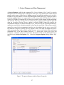
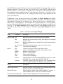
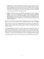
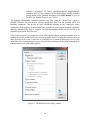
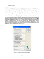
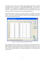
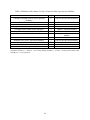
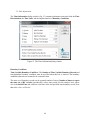
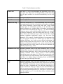
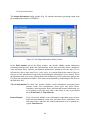
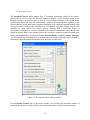
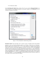
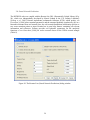
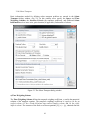
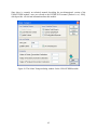
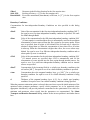
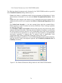
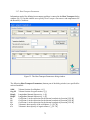
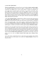
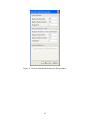
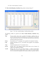
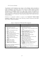
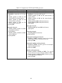
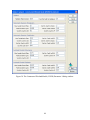
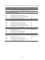
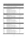
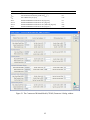
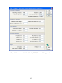
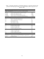
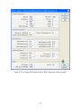
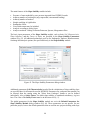
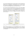
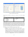
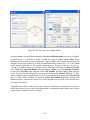
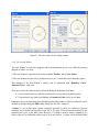
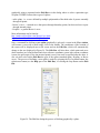
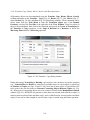
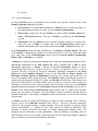
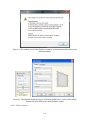
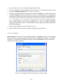
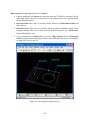
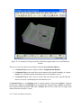
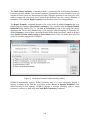
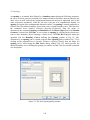
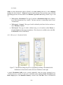
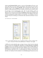
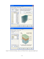
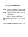
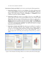
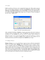
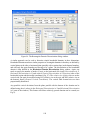
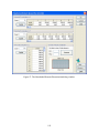
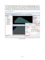
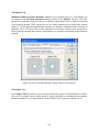
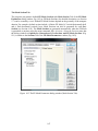
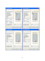
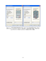
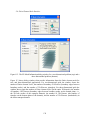
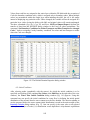
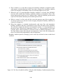
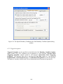
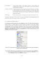
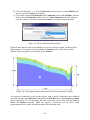
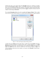
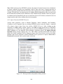
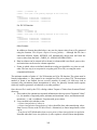
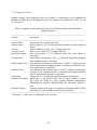
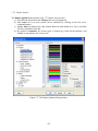
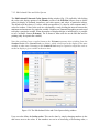
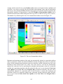
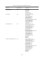
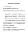
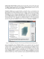
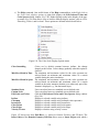
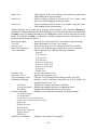
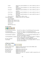
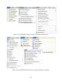
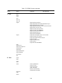
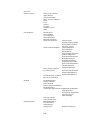
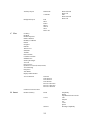
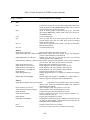
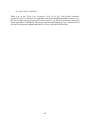
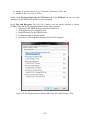
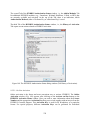
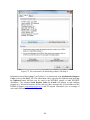
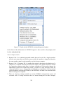
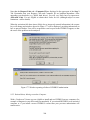
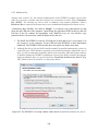
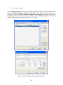
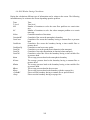
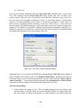
6. Domain Properties, Initial and Boundary Conditions
Initial and boundary conditions for both water flow and solute (heat) transport, and the spatial
distribution of other parameters characterizing the flow domain (e.g., the spatial distribution of soil
materials, hydraulic scaling factors, root-water uptake parameters, and possible hydraulic
anisotropy) and/or observation nodes are specified in a graphical environment with the help of a
mouse. The program automatically controls the logical correspondence between the water flow and
solute transport boundary conditions.
Various spatially variable properties (e.g., material distribution, initial and boundary conditions)
can be specified in Version 2.0 of HYDRUS (Standard and Professional, not Lite) either
a) directly on the finite element mesh (as done in Version 1.0), or
b) on geometric objects (e.g., boundary curves, rectangles, circles, surfaces, volumes).
The main advantage of the latter approach is that when the FEM is changed, these properties are
not automatically lost, but can be recalculated to the new FEM from their definition on
Geometric Objects. Which option is used depends on the menu command Edit->Properties and
Conditions on FE-Mesh. A similar button switch is also available at the end of the tool bar ( ),
next to the Results button, and at the Edit Bar. The latter approach (i.e., on Geometric Objects) is
described in detail below in Section 6.5.
6.1. Default Domain Properties
For rectangular two-dimensional domains and for layered three-dimensional domains,
immediately after the finite element mesh is generated, one can specify the initial Default
Domain Properties in the dialog window shown in Figure 115. Values listed in this window are
initially assigned to each horizontal layer of the transport domain, but can later be modified
graphically. The following variables are involved:
Code
h
Q
Mater
Roots
Axz
Bxz
Dxz
Temp
Conc
Sorb
Code of the boundary condition (0 for no flow, -1 for constant flux, +1 for constant
head, -2 for unsaturated seepage face, +2 for saturated seepage face, -3 (-7, -8, -9) for
variable flux, +3 (+7, +8, +9) for variable head, -4 for atmospheric, - 5 for tile drain, 6 for free drainage)
Initial value of the pressure head [L]. The initial pressure head changes linearly
between the first and last layer if one clicks on the command at the bottom of the
dialog (Linear interpolation of the pressure heads between the first and last layer).
Recharge flux, [L2T-1] and [L3T-1] for 2D and 3D applications, respectively. Since
this variable is usually specified in individual nodes, it is uncommon to specify it here.
Material number
Root distribution
Scaling factor for the pressure head
Scaling factor for the hydraulic conductivity
Scaling factor for the water content
Initial temperature [K]
Initial concentration (of the equilibrium phase) [ML-3]
Initial concentration of the nonequilibrium phase (kinetically sorbed [MM-1] or of the
immobile region [ML-3])
181