1
Ver. 1.2 May 2004
KLY- 4 / KLY- 4S / CS- 3 / CS- L
User’s Guide
Modular system for measuring magnetic susceptibility,
anisotropy of magnetic susceptibility,
and temperature variation of magnetic susceptibility.
AGICO
Advanced Geoscience Instruments Co.
Brno
Czech Republic
2
Contents
CONTENTS ................................................................................................................................................2
INTRODUCTION TO THE USER’S GUIDE ....................................................................................................4
PREFACE ...................................................................................................................................................4
WARRANTY ..............................................................................................................................................6
GENERAL SAFETY SUMMARY ............................................................................ 7
Convention .............................................................................................................................................................. 7
Injury Precautions.................................................................................................................................................... 7
Product Damage Precautions................................................................................................................................... 8
GETTING STARTED ................................................................................................ 9
KLY-4S / KLY-4 DESCRIPTION ...............................................................................................................9
KLY-4S / KLY-4 SPECIFICATIONS ........................................................................................................11
CS-3 / CS-L DESCRIPTION .....................................................................................................................12
CS-3 / CS-L SPECIFICATIONS.................................................................................................................12
EC DECLARATION OF CONFORMITY ......................................................................................................13
UNPACKING INSTRUCTIONS....................................................................................................................14
STORAGE AND TRANSPORTATION ..........................................................................................................14
INSTALLATION PROCEDURES.......................................................................... 15
Choosing the place ................................................................................................................................................ 15
Interconnection of Units ........................................................................................................................................ 15
Interconnection Scheme KLY-4 / CS-3 .................................................................................................................. 16
Testing the communication with computer............................................................................................................ 17
Testing the magnetic environment......................................................................................................................... 19
OPERATING BASICS ............................................................................................. 20
MEASURING OF AMS USING PROGRAM SUFAM................................................................................21
Purpose....................................................................................................................................................... 21
Running Program ....................................................................................................................................... 21
MEASURING MENU OF SUFAM ..............................................................................................................22
Function Key 1 15dir Sufam .................................................................................................................... 22
Measuring positions of the specimen SUFAM........................................................................................... 23
Function Key 2 Corr Sufam ..................................................................................................................... 25
Function Key 5 Eval Sufam ..................................................................................................................... 25
Function Key 6 ActVol Sufam.................................................................................................................. 30
Function Key 7 Help Sufam..................................................................................................................... 30
Function Key 9 Kill Sufam....................................................................................................................... 30
Function Key 10 Aux Sufam...................................................................................................................... 30
MEASURING OF AMS USING PROGRAM SUFAR................................................................................31
Purpose....................................................................................................................................................... 31
Running Program ....................................................................................................................................... 31
MEASURING MENU OF SUFAR ..............................................................................................................33
Function Key 1 Ax1 Sufar........................................................................................................................ 33
Measuring positions of the specimen SUFAR............................................................................................ 34
Function Key 2 Ax2 Sufar........................................................................................................................ 35
Function Key 3 Ax3 Sufar........................................................................................................................ 35
Function Key 4 Bulk3 Sufar..................................................................................................................... 35
Function Key 5 Field Sufar...................................................................................................................... 35
Function Key 5 Eval Sufar ....................................................................................................................... 36
Function Key 6 ActVol Sufar ................................................................................................................... 41
Function Key 7 Help Sufar ....................................................................................................................... 41
Function Key 8 Stop Sufar ....................................................................................................................... 41
Function Key 9 Kill Sufar........................................................................................................................ 41
3
Function Key 10 Aux Sufar....................................................................................................................... 41
AUXILIARY MENU OF SUFAR AND SUFAM .......................................................................................42
Convention ................................................................................................................................................. 42
Function AKey 1 Bulk ............................................................................................................................ 43
Function AKey 2 Etal Sufar.................................................................................................................... 43
Function AKey 2 Etal Sufam .................................................................................................................. 44
Function AKey 3 Cal Sufar ..................................................................................................................... 45
Function AKey 3 Cal Sufam ................................................................................................................... 46
Function AKey 4 Hol Sufar .................................................................................................................... 47
Function AKey 4 Hol Sufam................................................................................................................... 48
Function AKey 5 Orpar .......................................................................................................................... 49
Function AKey 6 Anfac .......................................................................................................................... 49
Function AKey 7 Help ............................................................................................................................ 50
Function AKey 8 Acmd Sufar ................................................................................................................. 50
Function AKey 8 Acmd Sufam ............................................................................................................... 50
Function AKey 9 Kill .............................................................................................................................. 50
Function AKey 10 Main ........................................................................................................................... 50
APPENDICES............................................................................................................ 51
LIST OF MAGNETIC ANISOTROPY FACTORS ...........................................................................................52
STRUCTURES OF DATA FILES.................................................................................................................53
Structure of Standard AMS File ................................................................................................................. 54
Structure of Geological Data File.............................................................................................................. 55
SELECTION OF COORDINATE SYSTEMS .................................................................................................56
GEOLOGICAL LOCALITY DATA...............................................................................................................57
MAINTENANCE ...................................................................................................... 58
Cleaning the Holder............................................................................................................................................... 58
Cleaning the Rotator.............................................................................................................................................. 58
KLY-4S Rotator - Belt Adjustment ................................................................... Chyba! Záložka není definována.
Cleaning the Up/Down Mechanism....................................................................................................................... 60
List of Error Messages of the System KLY-4S / CS-3 .......................................................................................... 61
APPARATUS CS-3 / CS-L ...................................................................................... 63
PREFACE .................................................................................................................................................64
CS-3 / CS-L DESCRIPTION .....................................................................................................................65
CS-3 / CS-L SPECIFICATIONS.................................................................................................................65
INSTALLING AND OPERATING THE CS-3 / CS-L ...................................................................................66
Furnace....................................................................................................................................................... 66
Temperature Sensor ................................................................................................................................... 66
Specimen .................................................................................................................................................... 67
Argon Flow Meter ...................................................................................................................................... 67
Measuring Vessel ....................................................................................................................................... 67
Cooling System .......................................................................................................................................... 68
Cryostat CS-L............................................................................................................................................. 69
MEASURING TEMPERATURE VARIATION OF MAGNETIC SUSCEPTIBILITY USING PROGRAM SUFTE ..70
Purpose....................................................................................................................................................... 70
Running the Program.................................................................................................................................. 70
Data File Description ................................................................................................................................. 76
MEASURING TEMPERATURE VARIATION OF MAGNETIC SUSCEPTIBILITY USING PROGRAM SUFTEL 77
Purpose....................................................................................................................................................... 77
Running the Program.................................................................................................................................. 77
4
Introduction to the User’s Guide
Thank you for purchasing magnetic susceptibility meter AGICO Kappabridge KLY-4.
Kappabridge and its optional accessories represent modular system designed for
measurement of magnetic susceptibility of rock and its anisotropy in variable fields, and
in conjunction with furnace or cryostat apparatus, also for measurement of temperature
variation of magnetic susceptibility.
Preface
The User’s Guide is divided into two parts.
❐
The Part 1, Kappabridge KLY-4 / KLY-4S, contains general common
information, description and specifications of individual modules, and decribes
the capabilities of the system. The attention is focused on measurement of
anisotropy of magnetic susceptibility (AMS) using the Kappabridge KLY-4S with
a spinning specimen and the KLY-4 version with static specimen.
❐
The Part 2, Apparatus CS-3 / CS-L, describes the measurement of temperature
variation of magnetic susceptibility using the high temperature furnace CS-3 and
low temperature cryostat CS-L.
5
KAPPABRIDGE
KLY- 4 / KLY- 4S
User’s Manual
Instrument for measuring magnetic susceptibility
and its anisotropy in variable fields
AGICO
Advanced Geoscience Instruments Co.
Brno
Czech Republic
6
Warranty
AGICO warrants that this product will be free from defects in materials and
workmanship for a period of 1 (one) year from date of installation. However, if the
installation is performed later than 3 (three) months after the date of shipment due to
causes on side of Customer, the warranty period begins three months after the date of
shipment. If any such product proves defective during this warranty period, AGICO, at
its option, either will repair the defective product without charge for parts and labour, or
will provide a replacement in exchange for the defective product.
In order to obtain service under this warranty, Customer must notify AGICO of the
defect before the expiration of the warranty period and make suitable arrangements for
the performance of service. AGICO will decide if the repair is to be performed by
AGICO technician or AGICO delegated serviceman in customers laboratory, or product
shall be sent for repair to the manufacturer. In latter case, customer shall be responsible
for packaging and shipping the defective product to the AGICO service centre. In both
cases, all the costs related to a warranty repair shall be at expenses of AGICO.
The warranty becomes invalid if the Customer modifies the instrument or fails to follow
the operating instructions, in case of failure caused by improper use or improper or
inadequate maintenance and care, or if the Customer attempts to install the instrument
without explicit written permission of AGICO company. AGICO shall not be obligated
to furnish service under this warranty a) to repair damage resulting from attempts by
personnel other than AGICO representatives to install, repair or service the product; b)
to repair damage resulting from improper use or connection to incompatible equipment;
or c) to service a product that has been modified or integrated with other products when
the effect of such modification increases the time or difficulty of servicing the product.
This warranty is given by AGICO with respect to this product in lieu of any other
warranties, expressed or implied. AGICO and its vendors disclaim any implied
warranties of merchantability or fitness for a particular purpose. AGICO’s responsibility
to repair or replace defective products is the sole and exclusive remedy provided to the
Customer for breach of this warranty. AGICO and its vendors will not be liable for any
indirect, special, incidental, or consequential damages irrespective of whether AGICO
or vendor has advance notice of the possibility of such damages.
7
General Safety Summary
Review the following safety precautions to avoid and prevent damage to this product or
any products connected to it.
Only qualified personnel should perform service procedures.
Convention
Symbol Attention is used to draw attention to a particular information.
Symbol Prohibition is used to accent important instruction, omission of which
may cause lost of properties, damage or injury.
Injury Precautions
Use Proper Power Cord. To avoid fire hazard, use only the power cord specified for
this product.
Do Not Operate Without Covers. To avoid electric shock or fire hazard, do not
operate this product with covers or panels removed.
Fasten Connectors. Do not operate the instrument if all connectors are not properly
plugged and fixed by screws.
Do Not Operate in Wet / Damp Conditions. To avoid electric shock, do not operate
this product in wet or damp conditions.
Do Not Operate in an Explosive Atmosphere. To avoid injury or fire hazard, do not
operate this product in an explosive atmosphere.
Disconnect Power Source. To avoid risk of electric shock unplug the instrument from
mains before reinstalling or removing unit.
8
Product Damage Precautions
Use Proper Power Source. Do not operate this product from a power source that
applies more than the voltage specified.
Use Proper Fuses only. Do not use fuses which are not specified by the manufacturer.
If a fuse with a different characteristics or value is used, the protection is not effective.
Operator’s Training. Operator should be familiar with operation of the instrument and
Safety Regulations.
Use Manufacturer’s Cables Only. Other devices can be connected to the instrument
via the appropriate cables only.
Do Not Disconnect Connectors. To avoid damage of the instrument never disconnect
any connector while device is on.
Do Not Operate With Suspected Failures. If you suspect there is damage to this
product, have it inspected by qualified service personnel.
9
Getting Started
In addition to a brief product description, this chapter covers the following topics:
❐
Specifications of Individual Modules.
❐
Declaration of Conformity.
❐
Unpacking Instructions.
❐
Storage and Transportation.
KLY-4S / KLY-4 Description
The KLY-4S / KLY-4 Kappabridge is probably the world's most sensitive
commercially available laboratory instrument for measuring bulk
magnetic
susceptibility and anisotropy of magnetic susceptibility (AMS). The Kappabridge has
the following features:
High sensitivity.
Automatic zeroing over the entire measuring range.
Autoranging.
Slowly spinning specimen (KLY-4S).
Quick AMS measurement (KLY-4S).
Easy manipulation.
Only three manual manipulations for measuring AMS (KLY-4S).
Built-in circuitry for controlling the furnace CS-3 and cryostat CS-L.
Full control by computer.
Sophisticated software support.
The Kappabridge apparatus consists of the Pick-Up Unit, Control Unit and User’s
Computer. In principle the instrument represents a precision fully automatic
inductivity bridge. It is equipped with automatic zeroing system and automatic
compensation of the thermal drift of the bridge unbalance as well as automatic
switching appropriate measuring range. The measuring coils are designed as 6th-order
compensated solenoids with a remarkably high field homogeneity.
10
The digital part of the instrument is based on micro-electronic components, with
the microprocessor controlling all functions of the Kappabridge. The instrument has
no control knobs, it is fully controlled by external computer via serial channel RS232C.
The KLY-4 version measures the AMS of a static specimen fixed in the manual holder.
In the static method, the same as in KLY-2 or KLY-3 bridges, the specimen
susceptibility is measured in 15 different orientations following rotatable design. From
these values six independent components of the susceptibility tensor and statistical
errors of its determination are calculated using software SUFAM. The specimen
positions are changed manually during measurement.
The KLY-4S version measures the AMS of a spinning specimen fixed in the rotator.
In the spinning method, the specimen rotates with small speed of 0.5 r.p.s. inside the
coil, subsequently about three axes. From these data, the deviatoric susceptibility tensor
can be computed. This tensor carries information only on anisotropic component of the
specimens. For obtaining complete susceptibility tensor one complementary
measurement of bulk susceptibility must be done.
The main advantage of the new model KLY-4 / KLY-4S is a possibility to measure bulk
susceptibility and AMS in variable fields from 3A/m to 450 A/m in 21 steps. The
autoranging and autozeroing work over the entire measuring range. Automatic zeroing
compensates real and imaginary components, the zeroing circuits work in digital way
using 16-bit up-down counters and D/A converters. The output signal is digitalized, raw
data are transferred directly to the computer which controls all the instrument functions.
These features enable to zero the bridge prior the anisotropy measurement after inserting
the specimen into the measuring coil. The ´background´ bulk susceptibility is eliminated
and the bridge measures only the susceptibility changes during specimen rotation and
thus the most sensitive range can be used. The result is high precision of measurement
and determination of principlal directions of susceptibility tensor.
One has to adjust the specimen only in three perpendicular positions. Thus the
specimen measurement time was dramatically shortened. The measurement is rapid,
about two minutes per specimen, and precise, profiting from many susceptibility
determinations in each plane perpendicular to the axis of specimen rotation. The static
method of the measurement can also be used.
Software SUFAR combines the measurements in three perpendicular planes plus one
bulk value to create a complete susceptibility tensor. The errors in determination of
this tensor are estimated using a new method based on multivariate statistics principle.
11
KLY-4S / KLY-4 Specifications
1
Specimen Size
Cylinder
Diameter
Length
Cube
Cube
ODP box
Fragments (bulk. susc.)
Spinning Specimen
25.4 mm (+0. 2 , -1. 5)
22.0 mm (+0. 5 , -1. 5)
Static Specimen
25.4 mm (+1. 0, -1. 0)
22.0 mm (+2. 0, -2. 0)
20 mm (+0. 5 ,
20 mm (+0.5 , -2. 0)
23 mm (+0.5 , -2. 0)
26 x 25 x 19.5 mm3
40 cm3
Pick-up coil inner diameter
Nominal specimen volume
Operating frequency
Field intensity
Field homogeneity
Measuring range
Sensitivity (300 Am-1) Bulk measurement
AMS measurement (spinning specimen)
Accuracy within one range
Accuracy of the range divider
Accuracy of the absolute calibration
HF Electromagnetic Field Intensity Resistance
Power requirements
Power consumption
Operating temperature range
Relative humidity
Dimensions / Mass
Measuring Unit
Pick-up Unit
Rotator
1
Holders for specimens of slightly different size can be supplied on request.
-1. 5)
43 mm
10 cm3
875 Hz
3 Am-1 to 450 Am-1 in 21 steps
0.2 %
0 to 0.2 (SI)
3 x 10⁻⁸ (SI)
2 x 10⁻⁸ (SI)
0.1 %
0.3 %
3%
1 Vm-1
240, 230, 120, 100 V ±10 %
50 / 60 Hz
45 VA
o
+ 15 to + 35 C
max. 80 %
260 mm x 160 mm x 250 mm / 4 kg
240 mm x 320 mm x 330 mm / 11 kg
320 mm x 70 mm x 65 mm / 1 kg
12
CS-3 / CS-L Description
The CS-3 Temperature Control Unit has been designed for measurement, in
connection with the KLY-4S Kappabridge, of the temperature variation of low-field
magnetic susceptibility of minerals, rocks and synthetic materials in the temperature
range from ambient temperature to 700 oC. The apparatus consists of non-magnetic
Furnace with a special platinum Thermometer, electronic Temperature Control Unit,
cooling water Reservoir with Pump, and Argon Flow Meter. The specimen is placed in a
measuring vessel which is heated by a platinum wire in three selectable heating rates.
The temperature is measured by special platinum thermometer. The protect Argon
atmosphere during heating can be applied to prevent oxidation of measured specimen.
To perform susceptibility measurement at a chosen temperature range, the equipment
moves automatically the furnace into and out of the pick-up coil of the KLY-4S
Kappabridge. The quasi-continuous measurement process is fully automated, being
controlled by the software SUFTE.
The CS-L Low Temperature Apparatus has been designed for measurement, in
connection with the KLY-4S Kappabridge and CS-3 Temperature Control Unit, of the
temperature variation of low-field magnetic susceptibility of minerals, rocks and
synthetic materials in the temperature range from minus 192 oC to ambient temperature.
The apparatus consists of non-magnetic Cryostat with a special platinum Thermometer.
The specimen is placed in a measuring vessel which is cooled inside the cryostat by
liquid nitrogen and then heated spontaneously to a given temperature. The argon gas is
needed for deplenishing the liquid nitrogen out of cryostat. Temperature is measured by
special platinum thermometer. The quasi-continuous measurement process, after cooling
the specimen, is fully automated, being controlled by the software SUFTEL.
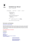
CS-3 / CS-L Specifications
3
Maximum specimen volume (fragments or powder)
Inner diameter of measuring vessel
Sensitivity to susceptibility changes (300 Am-1)
Temperature range CS-3
Temperature range CS-L
Accuracy of temperature sensor
Power requirements
Power consumption
Dimensions / Mass
Electronic unit
Water container with Pump
Argon flow meter
0.25 cm
6.5 mm
1 x 10 -7 (SI)
o
ambient temperature to 700 C
-192 oC to ambient temperature
o
±2 C
240, 230, 120, 100 V ±10 %, 50 / 60 Hz
350 VA
260 mm x 160 mm x 250 mm
380 mm x 380 mm x 700 mm
32 mm x 32 mm x 140 mm
Cryostat
Argon gas flow requirement (protect atmosphere)
Amount of liquid nitrogen (cooling cryostat)
Argon gas flow requirement (deplenishing cryostat)
diameter 60 mm, length 220 mm / 0.5 kg
approx. 100 ml min-1
approx. 0.5 l for one cooling
approx. 20 l min-1 for about 10 s
/ 9 kg
/ 2 kg
/ 1 kg
13
EC Declaration of Conformity
We,
AGICO, s.r.o., Ječná 29a, CZ - 621 00 Brno, IČO 607 313 54,
declare that the Modular system for measuring magnetic susceptibility, anisotropy of magnetic
susceptibility and temperature variation of magnetic susceptibility,
KLY-4
indicator of susceptibility and anisotropy of susceptibility,
KLY-4S
indicator of susceptibility and anisotropy of susceptibility with rotating sample,
CS-3
indicator of temperature variation of susceptibility from room temperature to 700 oC,
CS-L
indicator of temperature variation of susceptibility from –192 oC to room temperature,
meet the intent of directives 89/336 EEC and 73/23 EEC.
The compliance was demonstrated to the following specifications:
ČSN EN 61010-1+A2:1997 (EN 61010-1+A2:1995), ČSN EN 55022:1999 (EN 55022:1998),
ČSN EN 61326-1:1999 (EN 61326-1+A1:1998), ČSN EN 61000-4-2:1997 (EN 61000-4-2:1995),
ČSN EN 61000-4-3:1997 (EN 61000-4-3:1995), ČSN EN 61000-4-4:1997, (EN 61000-4-4:1995),
ČSN EN 61000-4-5:1997 (EN 61000-4-5:1995), ČSN EN 61000-4-6:1997 (EN 61000-4-6:1995),
ČSN EN 61000-4-11:1997 (EN 61000-4-11:1995).
Marking CE: 02
Manufacturer : AGICO, s.r.o., Ječná 29a, CZ - 621 00 Brno.
The judgement of conformity was performed in co-operation with the ITI TÜV s.r.o. Modřanská 98,
CZ – 147 00 Praha 4.
Place and date of issue: Brno, 23 April 2004.
Responsible person: Prof. RNDr. František Hrouda, CSc., director of company.
14
Unpacking Instructions
Remove carefully the instrument and its accessories from the box and packing material,
referring to the packing list included to confirm that everything has been delivered.
Briefly inspect each item for shipping damage. If anything is missing or damaged,
contact the manufacturer or your dealer immediately. You may want to retain the box
and other packing material in case later you need to ship the instrument.
Storage and Transportation
The properly wrapped instrument can be stored and transported at a temperature -20 oC
to + 55 oC and relative humidity up to 80 %. In both cases the instrument should be
stored in suitable premises, free of dust and chemical evaporation.
15
Installation Procedures
The first installation and training is performed exclusively by the AGICO technician or
by the authorised representatives. If you need later to reinstall the apparatus, due to the
removing the instrument to another place or any other reasons, be sure the following
conditions are met to achieve guaranteed parameters.
Choosing the place
Place the apparatus to a room with relatively magnetically clean environment.
The instrument must not be placed near sources of alternating magnetic field, e.g.
big transformers, electric motors, electricity power source wires, thermal sources
etc.
Do not place the instrument near thermal and electrical sources and prevent
the pick-up coils from direct sunshine. The pick-up coils must not be exposed to
heat from the sun or from other sources, which would affect the precision of
measurement.
Do not place the pick-up coils near the other instruments or computer’s
monitors.
Do not place the instrument to a draughty room. Air condition may sometimes
cause higher thermal drift of coils, prevent the direct air flowing in the room .
The temperature in the room should be stable as much as possible. The
temperature variation in the room should not exceed 2 oC / hour.
Place the instrument and pick-up unit on a wooden table with good stability which
has no iron loop under working desk.
It is recommended to place the pick-up unit on a separate stand or a small table
which should be of such a height so that the middle of the pick-up unit coincides
with the level of the working table. This arrangement makes the operation easier.
During measurement prevent motion of magnetically significant parts (metal parts
of chairs, doors, furniture, watches, rings, tools, components of your clothes, etc.)
Interconnection of Units
Fig. 1 shows the Interconnection Scheme. If you are installing only Kappabridge do not
care CS-3 unit and its accessories. Be sure the instrument is unplugged from mains
during connecting the cables. Fix the connectors by screws, plug the mains socket and
switch the Kappabridge on.
16
Interconnection Scheme KLY-4 / CS-3
17
Testing the communication with computer
Copy the software SUFAR and SUFAM (for KLY-4) to your computer exactly in
the same structure as it is on original diskette and run program SUFAR.EXE or
SUFAM.EXE.
After the program is started the communication of the instrument with your
computer via serial channel RS-232C is tested automatically each time you run the
program SUFAR or SUFAM. If there is something wrong in the communication,
the following message appears on the screen :
#### RS-232 COMMUNICATION ERROR
Current communication port: COM1
For change edit the file SUFAR.SAV
In this case it is recommended to switch the instrument off and to check the
connection of the instrument with the computer as well as to check whether the
correct serial port number is set in the configuration file SUFAR.SAV or
SUFAM.SAV.
If the number of the serial channel should be changed, it can be done using any
text editor (for example the NORTON Commander).
One must be very careful in this operation, because the SUFAR.SAV file is the
random access file and the port number must be changed only through
overwriting the number, but without affecting the other information contained in
the file and retaining the original format of the file. Then, the program should be
started once again after switching on the instrument.
If the communication is O.K., the following information subsequently appear
on the screen of the computer :
SUFAR program :
In case the initialization of the Up/Down Mechanism, of the Rotator and the
Zeroing of the bridge were successful :
Initialization in progress...
** LEVEL SET
** AUTO RANGE
** FIELD SET H = 300 A/m
Zeroing in progress ...
** END OF ZEROING
** READY
18
SUFAM program :
In case the Zeroing of the bridge was successful :
** AUTO RANGE
** FIELD SET H = 300 A/m
Zeroing in progress ...
** END OF ZEROING
These information inform the user of the current activities of the instrument. In
case the communication test was successful, and there are no other problems, the
offer of the MAIN MANU appears. For detailed information and explanation of
the main menu see chapter Operating Basics. Press <Ctrl Q> to quit the program.
In the case that something fails during initialization for some reasons (for
example, too strong disturbing magnetic fields in the vicinity of the pick up coil)
the following message appears :
FATAL ERROR
E7 ZEROING ERROR (blinking)
Press any key to return to AUX menu
If you wish to finish the program press <Ctrl Q> .
19
Testing the magnetic environment
Connect the multimeter (using a single two-wire cable - it is in the holder box) to
the KLY-4S control unit rear panel.
Run program SUFAM.EXE or SUFAR.EXE.
In the MAIN menu select function Key 10 AUX, then function Key 8 Acmd and
start the zeroing process by pressing <Z>. (During zeroing you can hear the sound
whose frequency is approximately proportional to the level of unbalance of the
bridge).
Immediately after and only after you obtain message ** END OF ZEROING, read
the voltage level on the multimeter. This voltage is approximately proportional to
the level of magnetic environmental background, should not be higher than 1 Volt
and should not be changing quickly.
If you do not use notebook with LCD display (we recommend it), take attention to
your PC monitor. The monitor distance from pick-up coils and its azimuth
position can have sometimes great influence. Try to rotate the monitor and/or
pick-up coils about the vertical axis, zero the bridge again, read the voltage value
on multimeter. Repeat several times and try to find the best configuration, when
the voltage value is minimal. Usually it is possible to obtain about 0.5 V, but there
is no reason to be nervous if it is higher but below 1 V.
20
Operating Basics
This chapter covers the following topics:
❐ Measuring of AMS using KLY-4 and program SUFAM
Measuring Menu of the SUFAM
❐ Measuring of AMS using KLY-4S and program SUFAR
Measuring Menu of the SUFAR
❐ Auxiliary Menu of the SUFAM and SUFAR
❐ Appendices
List of Magnetic Anisotropy Factors
Structures of Data Files
Selection of Coordinate Systems
Geological Locality Data
21
Measuring of AMS Using Program SUFAM
Purpose
This program serves for on line measurement of the anisotropy of magnetic
susceptibility of rocks using the KLY-4 Kappabridge (static specimen method).
During measurement process, the susceptibility of the specimen is measured
subsequently in 15 directions following the rotatable design in exactly the same way
as in the KLY-2 or KLY-3 Kappabridges. Using the least squares method, the
susceptibility tensor is fit to these measurements of the 15 directional susceptibilities
and the errors of the fit are calculated. The results of the measurement, in the form of
various parameters derived from the susceptibility tensor and orientations of the
directions of the principal susceptibilities in various coordinate systems, are presented
on the screen, can be printed using the line printer or written on the disk. The tensor
elements together with orientations of mesoscopic foliations and lineations can be also
written on the disk (into standard AMS file which is binary random access file) from
where they can be read in advanced processing.
Running Program
After the SUFAM.EXE is started,
appears on the screen
<Ctrl Q>
the information how to terminate the program
EXIT ,
the communication of the instrument with the computer is tested and the bridge is
automatically zeroed.
If there is no zeroing problem, the offer of the MAIN MENU appears
1 15dir
2 Corr
3
4
5 Field
6 ActVol
7 Help
8
9 Kill
10 Aux
This menu serves for the measurement of the specimen using program SUFAM.
Do not forget to install the plastic cylinder into the coil before the measurement with
SUFAM program.
22
Measuring Menu of Sufam
The individual function keys start the following activities:
F1 - measurement of the AMS in 15 directions
F2 - correction (repetition) of current position
F5 - field set or
evaluation of the measured data (activated only after all measurements F1 are
completed)
F6 - setting up the actual volume of the measured specimen
F7 - invoking the HELP page
F9 - breaking the current activities and clearing current specimen data
F10 - activation of the AUXILIARY MENU
Function Key 1 15dir
Sufam
This procedure serves for the measurement of 15 directional susceptibilities. The design
of the 15 directions is shown in the Fig. 2. The position design is the same for the cubic
and cylindrical specimens. After pressing F1, the following picture appears on the
screen
DATA MEASURED
RESIDUALS
Next direction 1
Press <SpaceBar> to continue
One puts the specimen into the holder in the position 1 (see Fig. 2), presses the
SpaceBar key and waits the computer's beep. Then, one inserts the specimen into
the measuring coil from where one pulls it out after the second beep. Then, one
changes the specimen's position and continues analogously until all the 15
directional susceptibilities are measured.
23
24
The results look like in the following example
DATA MEASURED
RESIDUALS in %
30.41E-03
32.25E-03
31.54E-03
-0.12
-0.19
0.03
31.27E-03
31.42E-03
31.79E-03
-0.11
-0.13
0.05
30.60E-03
31.20E-03
32.63E-03
-0.13
-0.28
-0.12
30.44E-03
32.33E-03
31.60E-03
-0.02
-0.05
0.24
30.29E-03
31.45E-03
31.85E-03
-0.03
-0.02
0.22
Std. error :
Anisotropy test
:
356.1
Confidence angles :
1
2 Corr
3
4
322.9
135.6
5.1
2.0
3.3
5 Eval
6
7
8
9 Kill
0.18
10 Aux
The three columns DATA MEASURED show the values of 15 directional
susceptibilities measured. The data RESIDUALS represent the deviations of the
measured and fitted data. After fitting the susceptibility ellipsoid to the measured
data using the least squares method, the susceptibility in each measuring direction
is calculated from the fitted tensor and subtracted from the measured value; this is
the residual. The residuals are the lower the higher is the measuring accuracy
and better fit. Ideally, the residuals are as low as the measuring errors of individual
directional susceptibilities. Std. error is the mean value of the absolute values of
the residuals.
The quality of the measurement can be evaluated also from the values of
Anisotropy test and Confidence angles. The Anisotropy test values are the
values of the F-test for anisotropy/isotropy and for triaxial/rotational prolate and
for triaxial/rotational oblate ellipsoids. If the left value is higher than 3.48,
then the differences between the principal susceptibilities determined by
measurement compared to measuring errors are great enough that the specimen
can be considered anisotropic from the statistical point of view (on the 95 % level
of significance). If the central and right values are higher than 4.25, then the
ellipsoid is triaxial. The Confidence angles values are those of the angles
defining the statistical accuracy of the determination of the directions of the
individual principal susceptibilities on the 95 % level of significance (for more
details see AGICO Print No. 1).
Fig. 2 Measuring positions of the specimen
25
Function Key 2 Corr
Sufam
This key may be activated during and after the 15 directional susceptibilities are
measured (during the measurement pressing Corr sets the position number to the
current position minus one). It enables any imprecisely measured directional
susceptibility to be re-measured. After complete measurement and after pressing F2,
one has to input the Direction to be repeated and re-measure the corresponding
directional susceptibility. The proper specimen position should be prepared before
pressing F2 key. The re-measurements in various directions can be repeated until the
expected accuracy is reached.
Function Key 5 Eval
Sufam
This procedure evaluates the measured data through the determination of the
susceptibility tensor and its related parameters. Before this procedure is activated, it is
possible to repeat measurement of any of the 15 directional susceptibilities in order to
get the best data for the evaluation. After the evaluation is once started, neither of the
directional susceptibilities can be re-measured; only the whole specimen can be remeasured.
If the Eval procedure is started for the first time, the following questions
subsequently appear on the screen
Path ?
drive:\ dir1\dir2\...\ <CR>...current
Name of file ?
without extension, 8 chars max.
Each of associated files contains x record(s)
Specimen name (# means new file) ?
After the above information are input, the question appears for the way of inputting
the geological orientation data
➪
Select:
Using geological file
[1]
Manual input from memo-book
[2]
Non-oriented specimen
[3]
➪
One selects [1] if the data should be read from the geological data file created
earlier (the geological data file can be created using the program ANISOFT
program package) which is located in the same directory as the standard AMS file
being measured. The reading is made automatically by the computer. The
geological data are used in the calculations and also copied into the standard
AMS file (see Appendix 2).
➪
If one selects [2], the following questions appear on the screen
MANUAL INPUT FROM MEMO-BOOK
2 sampling angles ?
26
One inputs the angles of the orientation of the specimen, the first is azimuth of
the fiducial mark of the specimen, the second is the dip or plunge of the fiducial
mark, for details see the AGICO Print No. 6.
Number of tectonic systems (0 to 2):
If 0 is input (for example if non-foliated and non-lineated volcanic or plutonic
rock is measured), no other geological data are input.
If 1 or 2 is input, the following data must also be input
1: Code, 4 tectonic angles ?
The two-character code characterizes the measured mesoscopic foliation and
lineation, the angles are azimuth of the dip (or strike if the orientation parameter
P4 is 90), dip of the first mesoscopic foliation, trend, plunge of the first
mesoscopic lineation, respectively. If only foliation exists, the second character
in the code must be zero and the last two angles are also zeros.
If 2 is input, the following data must also be input
2: Code, 4 tectonic angles ?
The two-character code characterizes the measured mesoscopic foliation and
lineation, the angles are azimuth of the dip (or strike if the orientation parameter
P4 is 90), dip of the second mesoscopic foliation, trend, plunge of the second
mesoscopic lineation, respectively. If only foliation exists, the second character of
the code must be zero and the last two angles are also zeros.
➪
If one selects [3], no angle data are necessary.
After the geological data are input the program displays the results and after
pressing ESC key, the program asks
Output to file
[Y/N]
<CR> = YES
Output to printer
[Y/N]
<CR> = NO
These questions concern the calculated data which appear later on the screen.
They can be written to the file on the disk and/or on the paper using the line
printer. If they are written on the disk, they are written as an ASCII file in the
same format as they appear on the screen (later they can be re-printed on the
paper if necessary). The extension of this file is ASC and the file is located in the
same directory as the standard AMS file.
After measuring the second or later specimen only the question for the
specimen name appears on the screen. The data are handled in the same way as
those of the first specimen. If one wishes to change the file, one inputs #
instead of the specimen name and the inputting is made as in the first specimen.
27
Then, the calculated data are shown on the screen in the form whose example is
shown on the next page. The meaning of the presented results is as follows :
Azi
first orientation angle (mostly azimuth of the dip or strike of the
fiducial mark on the specimen)
Dip
second orientation angle (dip of the fiducial mark or plunge of
the cylinder axis)
O.P.
orientation parameters (see the section OrPar)
Nom.vol.
nominal volume of the used pick up unit (mostly 10cm3)
Act.vol.
the volume of the specimen measured (in cm3)
Demag.fac.
information whether the demagnetizing factor of the specimen
was considered in the calculation of the mean susceptibility
Holder
susceptibility of the holder (measured in the section Hol)
T1
code for the first pair of mesoscopic foliation and lineation
F1
orientation angles for the first foliation
L1
orientation angles for the first lineation
T2
code for the second pair of mesoscopic foliation and lineation
F2
orientation angles for the second foliation
L2
orientation angles for the second lineation
Mean
mean susceptibility
Norming factor
norming factor for calculation of the
normed susceptibility tensor
Standard err. [%]
error in fitting the susceptibility tensor of
the measured data
F, F12, F23
statistics for anisotropy, triaxiality and
uniaxiality testing
Normed principal susceptibilities
principal susceptibilities normed by the
norming factor and errors in their
determination
95% confidence angles, E12, E23, E13 confidence angles (on the 95 %
probability level) in the determination of
the orientations of the principal
susceptibilities
28
Anisotropy factors
values of
parameters
the
selected
anisotropy
Principal directions
orientations of principal susceptibilities
(in decreasing succession) as declination
(D) and inclination (I) in various
coordinate systems
Normed tensor
values of the normed susceptibility
tensor in the appropriate coordinate
system; the upper line gives the diagonal
tensor elements (consecutively K11,
K22, K33),while the lower line gives the
non-diagonal elements (K12, K23, K13)
29
NJC8-1
******
Azi
Dip
ANISOTROPY OF SUSCEPTIBILITY
30
60
T1
CD
O.P. : 12
0
3
Demag. fac. : NO
90
Holder -5.15E-06
L1
30/40
T2
SO
F1
100/20
Field
[A/m]
300
Program SUFAM ver.1.0
Mean
susc.
199.2E-06
Standard
err. [%]
0.22
F2
140/60
F
271.2
Normed principal
Nom. vol. 10.00
Act. vol. 8.00
L2
70/80
Tests for anisotropy
F12
F23
33.9
363.7
95% confidence angles
susceptibilities
1.0323
1.0139
0.9537
+- 0.0014
0.0014
0.0014
E12
E23
E13
10.1
3.1
2.4
Anisotropy factors (principal values positive)
L
F
P
'P
T
U
Q
E
1.018
1.063
1.082
1.087
0.546
0.532
0.265
1.044
Principal directions
241
76
344
4
3
85
Normed tensor
0.9591
1.0115
1.0294
0.0166 -0.0041 -0.0080
Specimen
system
D
I
Geograph
system
D
I
164
63
278
11
13
24
0.9695
-0.0119
1.0117
-0.0029
1.0188
-0.0288
Paleo 1
system
D
I
127
51
264
31
8
21
0.9654
0.0162
1.0176
0.0094
1.0169
0.0074
Tecto 1
system
D
I
187
51
324
31
68
21
1.0141
0.0173
0.9690
0.0211
1.0169
-0.0151
Paleo 2
system
D
I
91
5
187
47
356
43
0.9818
0.0018
1.0320
0.0036
0.9862
-0.0368
Tecto 2
system
D
I
111
5
207
47
16
43
0.9865
-0.0126
1.0273
-0.0072
0.9862
-0.0294
➪ The data page can be left by pressing ESC key.
30
Function Key 6 ActVol
Sufam
This procedure serves for inputting the actual volume of the measured specimen. If all
the specimens measured in a particular collection have the same volume, it is sufficient
to input this volume only once. If the volume varies from specimen to specimen, it is
necessary, before or after the measurement of each specimen (but at least before the
evaluation of the measured data), to input the correct volume of the measured
specimen.
After starting this procedure, the volume written in the configuration file appears
on the screen in the following form :
Actual volume
ccm
10
Any changes [Y/N] ?
If the volume of the measured specimen is the same, one only hits ENTER, while
if the volume is different, one should input Y and then the actual volume of the
measured specimen.
Function Key 7 Help
Sufam
This key invokes the help procedure. To quit help page press ESC key.
Function Key 9 Kill
Sufam
This key breaks the current activities and clears the measured and input specimen data.
Function Key 10 Aux
This key switches the program to the AUXILIARY MENU.
Sufam
31
Measuring of AMS Using Program SUFAR
Purpose
This program serves for on line measurement of the anisotropy of magnetic
susceptibility of rocks using the KLY-4S Kappabridge (spinning specimen method).
During measurement, the specimen slowly rotates subsequently about three
perpendicular axes. The bridge is zeroed after inserting the specimen into the measuring
coil so that susceptibility differences are measured during specimen spinning (64
measurements are made during one spin) which results in very sensitive determination
of the anisotropic component of the susceptibility tensor profiting from the
measurement on the lowest possible and therefore most sensitive range. Then, one bulk
susceptibility value is measured along one axis and the complete susceptibility tensor is
combined from these measurements. The measured data, in the form of various
parameters derived from the susceptibility tensor and orientations of directions of the
principal susceptibilities in various coordinate systems, are presented on the screen, can
be printed using the line printer or written on the disk (into a sequential ASCII file). The
tensor elements together with orientations of mesoscopic foliations and lineations can be
also written on the disk (into standard AMS file which is binary random access file)
from where they can be read in advanced processing.
Running Program
After the SUFAR.EXE is started, the information how to terminate the program appears
on the screen
<Ctrl Q>
EXIT
and the communication of the instrument with the computer is automatically tested.
If communication failed check configuration file SUFAR.SAV (see also the
chapter Testing the communication with computer).
If the communication is O.K., the following information subsequently appear on
the screen of the computer
Initialization in progress...
** LEVEL SET
** AUTO RANGE
** FIELD SET H = 300 A/m
Zeroing in progress ...
32
** END OF ZEROING
** READY
These are information of the current activities of the instrument.
In the case that initialization or zeroing failed for some reasons (for example, too
strong disturbing magnetic fields in the vicinity of the pick up coil) the following
message appears
FATAL
ERROR
E7 ZEROING ERROR (blinking)
Press any key to abort program
1 Ax1
If there is no initialization or zeroing problem, the offer of the MAIN MENU
appears
2 Ax2
3 Ax3
4 Bulk3
5 Field 6 ActVol
7 Help
8 Stop 9 Kill
10Aux
This menu serves for the measurement of the specimen using program SUFAR.
Do not forget to remove the plastic cylinder from the coil in case the SUFAM program
was used in the last session.
33
Measuring Menu of SUFAR
The individual function keys start the following activities:
F1
the specimen spins about the x1 axis (measurement of the AMS in the x2,x3 plane
of the specimen - Position No.1)
F2
the specimen spins about the x2 axis (measurement of the AMS in the x2,x3 plane
of the specimen - Position No.2)
F3
the specimen spins about the x3 axis (measurement of the AMS in the x1,x2 plane
of the specimen - Position No.3)
F4
measurement of the bulk susceptibility in the Position No.3
F5
field set or evaluation of the measured data (activated only after the measurements
F1 to F4 are completed)
F6
setting up the actual volume of the measured specimen
F7
invoking the HELP page
F8
stops the current measurement and sets up the rotator to the initial position
F9
the program breaks the current activities and clears current specimen data
F10 activation of the AUXILIARY MENU
Function Key 1 Ax1
Sufar
This procedure serves for the measurement of the AMS in the x1,x2 plane (the specimen
spins about the x1 axis). The spinning is very slow (one revolution per 2 seconds) and
the susceptibility is measured 64 times during one revolution. As the bridge is zeroed
with the specimen inserted into the measuring coil before the specimen starts spinning,
the susceptibility differences are measured between the susceptibilities along the
respective directions and that of the direction in which the bridge was zeroed. This way
of measurement is very advantageous, because one measures only the anisotropic
component of the susceptibility which is much lower than the bulk component and one
can profit from the higher accuracy of the measurement made on the more sensitive
range.
Before pressing Key F1, one has to fix the specimen into the specimen holder in
the measuring position No. 1 (see Fig. 3).
After pressing F1, the specimen is inserted into the specimen coil, the bridge is
zeroed and the specimen starts spinning; during spinning the specimen
susceptibility is measured.
34
Measuring positions of the specimen
SUFAR
Fig. 3 Measuring positions of the specimen
The results are presented in the form as in the following example
Ax
1
Range
Cosine
Sine
Error
Error%
1
-5.709E-06
-2.102E-06
8.2E-09
0.14
Ax means that the specimen spinned about the x1 axis (the measurement was
made in the x2,x3 plane - Position No.1).
Range informs us of the range on which the anisotropy was measured (this is only
formal information, because the instrument has a fully autoranging feature).
Cosine and Sine give the values of the cosine and sine components, respectively,
of the average anisotropy curve.
Error gives the standard deviation of the individual curves from the average
curve.
Error% gives this deviation divided by the amplitude value.
35
The Error you obtain in each of three AMS axes measurement is standard deviation of
the individual curves (there are two sine wave curves for one physical revolution) from
the average curve and the Error% gives this deviation divided by the amplitude value.
This errors has only informative meaning and reflect the ratio between the noise and
aniso signal for measurement in one plane only. Thus it depends not only on absolute
susceptibility of the specimen measured but mainly on the degree of anisotropy in an
individual plane perpendicular to the axis of rotation. In case there is no anisotropy in
one of the three planes this error may be over 100% and has no physical meaning. In
case the anisotropy in one plane has "reasonable" value, the usual value is lower 5%, but
it does not reflect the quality of the measurement, but the level of anisotropy in one
plane. On the other hand it is clear that the sensitivity of the instrument influeces this
error. For judgement of the quality of AMS measurement, use F test numbers and 95%
confidence angles. The general rule is follow. If the F numbers are high (let say at least
above 5) the confidence angles are low and principal direction (directions) is (are) very
well defined. The sensitivity of AMS measurement for field 300 Am-1 on KLY-4S is
2x10⁻⁸, the anisotropy of the specimens with mean susc. about 5x10⁻⁶ SI can be
measured, but the confidence angles may be in some cases higher, it depends on type of
anisotropy.
Function Key 2 Ax2
Sufar
This procedure serves for the measurement of the AMS in the x1,x3 plane (the specimen
spins about the x2 axis - Position No.2 ) in the same way as in the previous case.
Function Key 3 Ax3
Sufar
This procedure serves for the measurement of the AMS in the x1,x2 plane (the specimen
spins about the x3 axis - Position No.3 ) in the same way as in the previous case.
Function Key 4 Bulk3
Sufar
This procedure measures the bulk susceptibility along the x1 axis (corresponding to the
specimen in the third measurement position). After pressing F4, the bridge is zeroed, the
specimen is inserted into the measuring coil and the bulk susceptibility is measured.
The knowledge of the bulk susceptibility along the x1 axis is necessary in the
construction of the complete susceptibility tensor from the deviatoric tensor (based
on susceptibility differences) and one bulk value
Function Key 5 Field
Sufar
After pressing the Fkey the required Field can be entered. The value is automatically
rounded into the row of 21 available Fields. Below 10 A/m in step of 2 A/m, upper 10
A/m up to 100 A/m in step of 10 A/m and upper 100 A/m up to 450 A/m in step of 50
A/m.
36
Function Key 5 Eval
Sufar
This procedure evaluates the measured data through the determination of the
susceptibility tensor and its related parameters. Before this procedure is activated, it is
possible to repeat any of the procedures Ax1, Ax2, Ax3, Bulk3 in order to get the best
data for the evaluation. When any of the above procedures is completed, the denotation
of the respective key is supplemented by an asterisk *. After the evaluation is once
started, neither of the above procedures can be repeated; only the whole specimen can
be re-measured.
If the Eval procedure is started for the first time, the following questions
subsequently appear on the screen
Path ?
drive:\ dir1\dir2\...\ <CR>...current
Name of file ?
without extension, 8 chars max.
Each of associated files contains x record(s)
Specimen name (# means new file) ?
After the above information are input, the question appears for the way of inputting
the geological orientation data
➪
Select:
Using geological file
[1]
Manual input from memo-book
[2]
Non-oriented specimen
[3]
➪
One selects [1] if the data should be read from the geological data file created
earlier (the geological data file can be created using the ANISOFT program
package) which is located in the same directory as the standard AMS file being
measured. The reading is made automatically by the computer. The geological
data are used in the calculations and also copied into the standard AMS file (see
Appendix 2).
➪
If one selects [2], the following questions appear on the screen
MANUAL INPUT FROM MEMO-BOOK
2 sampling angles ?
One inputs the angles of the orientation of the specimen, the first is azimuth of
the fiducial mark of the specimen, the second is the dip or plunge of the fiducial
mark, for details see the AGICO Print No. 6.
Number of tectonic systems (0 to 2):
If 0 is input (for example if non-foliated and non-lineated volcanic or plutonic
rock is measured), no other geological data are input.
37
If 1 or 2 is input, the following data must also be input
1: Code, 4 tectonic angles ?
The two-character code characterizes the measured mesoscopic foliation and
lineation, the angles are azimuth of the dip (or strike if the orientation parameter
P4 is 90), dip of the first mesoscopic foliation, trend, plunge of the first
mesoscopic lineation, respectively. If only foliation exists, the second character
in the code must be zero and the last two angles are also zeros.
If 2 is input, the following data must also be input
2: Code, 4 tectonic angles ?
The two-character code characterizes the measured mesoscopic foliation and
lineation, the angles are azimuth of the dip (or strike if the orientation parameter
P4 is 90), dip of the second mesoscopic foliation, trend, plunge of the second
mesoscopic lineation, respectively. If only foliation exists, the second character of
the code must be zero and the last two angles are also zeros.
➪
If one selects [3], no angle data are necessary.
After the geological data are input the program displays the results and after
pressing ESC key, the program asks
Output to file
[Y/N]
<CR> = YES
Output to printer
[Y/N]
<CR> = NO
These questions concern the calculated data which appear later on the screen.
They can be written to the file on the disk and/or on the paper using the line
printer. If they are written on the disk, they are written as an ASCII file in the
same format as they appear on the screen (later they can be re-printed on the
paper if necessary). The extension of this file is ASC and the file is located in the
same directory as the standard AMS file.
After measuring the second or later specimen only the question for the
specimen name appears on the screen. The data are handled in the same way as
those of the first specimen. If one wishes to change the file, one inputs #
instead of the specimen name and the inputting is made as in the first specimen.
Then, the calculated data are shown on the screen in the form whose example is
shown on the next page. The meaning of the presented results is as follows :
38
Azi
first orientation angle (mostly azimuth of the dip or strike of the
fiducial mark on the specimen)
Dip
second orientation angle (dip of the fiducial mark or plunge of
the cylinder axis)
O.P.
orientation parameters (see the section OrPar)
Nom.vol.
nominal volume of the used pick up unit (mostly 10cm3)
Act.vol.
the volume of the specimen measured (in cm3)
Demag.fac.
information whether the demagnetizing factor of the specimen
was considered in the calculation of the mean susceptibility
Holder
susceptibility of the holder (measured in the section Hol)
T1
code for the first pair of mesoscopic foliation and lineation
F1
orientation angles for the first foliation
L1
orientation angles for the first lineation
T2
code for the second pair of mesoscopic foliation and lineation
F2
orientation angles for the second foliation
L2
orientation angles for the second lineation
Mean
mean susceptibility
Norming factor
norming factor for calculation of the
normed susceptibility tensor(equal to the
absolute
value
of
the
mean
susceptibility)
Standard err. [%]
error in fitting the susceptibility tensor of
the measured data
F, F12, F23
statistics for anisotropy, triaxiality and
uniaxiality testing
Normed principal susceptibilities
principal susceptibilities normed by the
norming factor and errors in their
determination
95% confidence angles, E12, E23, E13 confidence angles (on the 95 %
probability level) in the determination of
the orientations of the principal
susceptibilities
39
Anisotropy factors
values of
parameters
the
selected
anisotropy
Principal directions
orientations of principal susceptibilities
(in decreasing succession) as declination
(D) and inclination (I) in various
coordinate systems
Normed tensor
values of the normed susceptibility
tensor in the appropriate coordinate
system; the upper line gives the diagonal
tensor elements (consecutively K11,
K22, K33),while the lower line gives the
non-diagonal elements (K12, K23, K13)
40
9-4-1
*****
Azi
Dip
ANISOTROPY OF SUSCEPTIBILITY
30
60
T1
CD
O.P. : 12
0
3
Demag. fac. : NO
90
Holder -1.67E-06
L1
30/40
T2
SO
F1
100/20
Field
[A/m]
300
Program SUFAR ver.1.0
Mean
susc.
127.9E-06
Standard
err. [%]
0.042
Nom. vol. 10.00
Act. vol. 11.00
F2
140/60
L2
70/80
Tests for anisotropy
F
F12
F23
2953.2
2055.3
1564.5
Normed principal
95% confidence angles
susceptibilities
Ax1
Ax2
Ax3
1.0304
0.9985
0.9711
1.6
1.9
0.9
+- 0.0003
0.0003
0.0003
0.9
1.6
1.9
Anisotropy factors (principal values positive)
L
F
P
'P
T
U
Q
E
1.032
1.028
1.061
1.061
-0.063
-0.078
0.738
0.996
Principal directions
283
193
68
4
3
85
Normed tensor
1.0000
1.028
0.9715
-0.0069
0.0046
0.0004
Specimen
system
D
I
Geograph
system
D
I
40
9
146
60
305
28
1.0095
0.0254
0.9973
0.0124
0.9932
-0.0028
Paleo 1
system
D
I
34
26
152
44
284
35
1.0153
0.0162
0.9890
0.0194
0.9957
0.0074
Tecto 1
system
D
I
94
26
212
44
344
35
0.9815
0.0033
1.0228
0.0161
0.9957
-0.0131
Paleo 2
system
D
I
229
67
42
23
133
2
0.9878
0.0160
0.9868
-0.0095
1.0254
-0.0068
Tecto 2
system
D
I
249
67
62
23
153
2
0.9774
0.0126
0.9972
-0.0112
1.0254
-0.0031
➪ The data page can be left by pressing ESC key
41
Function Key 6 ActVol
Sufar
This procedure serves for inputting the actual volume of the measured specimen. If all
the specimens measured in a particular collection have the same volume, it is sufficient
to input this volume only once. If the volume varies from specimen to specimen, it is
necessary, before or after the measurement of each specimen (but at least before the
evaluation of the measured data), to input the correct volume of the measured
specimen.
After starting this procedure, the volume written in the configuration file appears
on the screen in the following form :
Actual volume
ccm
10
Any changes [Y/N] ?
If the volume of the measured specimen is the same, one only hits ENTER, while
if the volume is different, one should input Y and then the actual volume of the
measured specimen.
Function Key 7 Help
Sufar
This key invokes the help procedure. To quit help page press ESC key.
Function Key 8 Stop
Sufar
This key stops the current measurement and sets up the rotator to the initial position.
Function Key 9 Kill
Sufar
This key breaks the current activities and clears the measured and input specimen data.
Function Key 10 Aux
This key switches the program to the AUXILIARY MENU.
Sufar
42
Auxiliary Menu of SUFAR and SUFAM
This menu is usually used to input the auxiliary information into the program useful
during the measurement of all the specimens in one measuring shift.
Convention
To help you quickly find the information, the name of the Key of the Auxiliary Menu is
denoted as Function AKey, instead of Function Key in Measuring (Main) Menu, to
underline that the key of Auxiliary menu is mentioned. Examples of measurement
values are expressed in Italic.
After activating Auxiliary menu, the following offer appears in SUFAR program
1 Bulk
2 Etal
3 Cal
4 Hol
5 Orpar
6 Anfac
7 Help
8 Acmd
9 Kill
10 Main
In the program Sufam the menu is the same.
The individual keys start the following procedures:
F1
measurement of the bulk susceptibility only (without AMS) of a specimen. It can
be useful in susceptibility monitoring between demagnetization steps in
palaeomagnetism.
F2
checking and/or inputting the susceptibility value for the used calibration standard
F3
instrument calibration
F4
measurement of the susceptibility of the specimen holder
F5
checking and/or setting up the values of the orientation parameters
F6
checking and/or setting up the set of the parameters characterizing the rock AMS
F7
invoking the help procedure
F8
auxiliary commands
F9
-
Enable and Disable movement Up/Down
(available for KLY-4S)
-
checking the Up and Down movement
(available for KLY-4S)
-
Zeroing of the bridge
-
Field set
-
List of Parameters
the program breaks the current activities
F10 return to the MAIN MENU
43
Function AKey 1 Bulk
This procedure serves for measurement of the bulk susceptibility (for example in
monitoring the susceptibility changes due to the demagnetization steps in
palaeomagnetism).
After starting the procedure, the following information appear on the screen :
Measurement of bulk susceptibility
----------------------------------------------The current holder susceptibility : -2.57 E-6
New measurement of holder [Y/N] ?
If one inputs Y, the procedure Key 4 Hol is made. If one inputs N or <CR>, the
procedure continues by bulk measurement in current Field - select <F>, or by
measurement of the bulk field variation Curve in all available fields - select <C>.
In case of individual bulk measurement any measurement is started by pressing
Then the bridge is zeroed, wait for a beep and insert (KLY-4 only) the
specimen into the pick-up coil, wait for second beep and pull (KLY-4 only) the
specimen out.
<CR>.
To finish measurements, type Q
N
Specimen
Bulk
1
XY
-4.58E-06
2
STANDARD
82.75E-03
3
Q
After inserting the specimen into the specimen holder and inputting the specimen
name, the bulk susceptibility is measured using manual holder. The measurement
is terminated after inputting Q instead of the specimen name. The bulk
susceptibility is calculated using the specimen volume which is entered in
procedure Key 6 ActVol.
Function AKey 2 Etal
Sufar
This procedure serves for checking and setting the nominal values of the calibration
standard.
44
Please note that the instrument is calibrated by two values. This is because the
calibration standard gives not only the directional bulk susceptibility value, but
also the anisotropy which is derived from the susceptibility along the x3 axis of
the standard and from that along the direction perpendicular to the x3 axis.
After activating this procedure through pressing the AKey F2, the following
information appear on the computer screen.
Etalon
Bulk-max
136.7 E-03
Bulk-min
27.00 E-03
Any Changes [Y/N]
If both the Bulk-max and Bulk-min values are the same as those written on the
etalon to be used for the instrument calibration, one inputs N or <CR> and the
procedure is terminated.
If any or both the values are different, one has to input Y and then the correct
values of both the Bulk-max and Bulk-min. Then, the procedure is finished.
Note: If you change the calibration standard nominal value(s), the Holder is reset
to zero. (See AKey 3 and AKey 4).
Function AKey 2 Etal
Sufam
After activating this procedure through pressing the AKey F2, the following information
appear on the computer screen
Etalon
Susc.
136.7 E-03
(the higher value of the two written on the standard)
Any Changes [Y/N]
If the Susc. value is the same as the higher one written on the standard to be used
for the instrument calibration, one inputs N or <CR> and the procedure is
terminated.
If the value is different, one has to input Y and then the correct value. Then, the
procedure is finished.
Note: If you change the calibration standard nominal value, the Holder is reset to
zero. (See AKey 3 and AKey 4).
45
Function AKey 3 Cal
Sufar
This procedure serves for the calibration of the instrument. This calibration is made as
for the bulk susceptibility value along the x3 axis of the standard as well as for the
anisotropy represented by the susceptibility difference between the standard
susceptibility along the x3 axis and the perpendicular direction (the standard is fixed in
the holder in the first measuring position, see Fig. 3).
After activating this procedure through pressing the AKey F3, the calibration
procedure starts and the following information subsequently appear on the computer
screen
AUX
300 A/m
**
ANISO
CALIBRATION : 05-15-2003 08:13:47
Bulk
Cos
Sin
Delta
GainA
GainB
0.00 E+00
-22.77
1.0023
1.0005
OLD
136.7 E-03
54.85 E-03
MEAS
136.6 E-03
54.84 E-03
38.51E-06
-22.77
1.0023
1.0005
NEW
136.7 E-03
54.85 E-03
0.00 E+00
-22.81
1.0027
1.0008
➪ Press <CR> to save calibration data
Bulk displays the values of the bulk susceptibility of the standard along the x3
axis.
Cos shows the value of the cosine component of the anisotropy of the standard.
Sin shows the value of the sine component of the anisotropy of the standard.
Delta value represents the phase lag of the measured signal relatively to the
position of the spinning specimen. This lag is mainly due to the phase
characteristics of the output low-pass filter.
GainB is the correction for getting the total gain for the bulk susceptibility to be
measured precisely.
GainA is the correction for getting the total gain for the anisotropy to be measured
precisely.
The line headed “OLD” gives the above data of the last calibration corresponding
to those written in the configuration file.
The line “MEAS” gives the data actually measured standard assuming that Delta,
GainB and GainA values equal “OLD” values.
46
The line headed “NEW” shows the result of the above measurement, but with
proper new corrections Delta, GainB, GainA. The constants Delta, GainB, GainA
are also written into the configuration file.
The data are systematically checked to warn, if needed, the operator to prevent
writing results into the configuration file. Thus, the GainB and GainA values
should be within the interval of 90% to 110% of the old values, otherwise the
error is indicated.
Note: If you change the calibration standard nominal value, the GainB and GainA
are undefined for current field until proper calibration is performed successfully.
Function AKey 3 Cal
Sufam
This procedure serves for the calibration of the instrument. After pressing AKey F3, the
following message appear :
Calibration in current Field
➪ Insert calibration standard after first (longer) beep
... Pull out it after second (shorter) beep
Press <SPACE> bar if you are ready to continue
Before pressing any key, it is necessary to put the standard into the holder in such
a way that the cylinder axis is vertical and after pressing space bar one has to
follow the above instructions.
The calibration results are shown as follows
AUX
300 A/m
CALIBRATION : 05-15-2003 08:13:47
OLD
Bulk
Gain
136.7 E-03
1.0001
MEAS 136.5 E-03
NEW
1.0001
136.7 E-03
➪ Press <CR> to save calibration data
1.0016
** BULK
47
The column Bulk displays the values of the bulk susceptibility of the standard
along the x3 axis. Gain is the correction for getting the total gain for the bulk
susceptibility to be measured precisely.
Note: If you change the calibration standard nominal value, the Gain is undefined
for current field until proper calibration is performed successfully.
Function AKey 4 Hol
Sufar
This procedure consists of the measurement of the bulk susceptibility and anisotropy of
the empty holder in the field 300 A/m. This susceptibility and anisotropy are written
into the configuration file and subtracted from the measured values after measuring the
specimen.
After activating this procedure through pressing the AKey F4, the measurement of
the empty holder starts and the following information subsequently appear on the
computer screen
AUX
HOLDER
Old values
New values
Std.error
Bulk
300 A/m
Cos
Sin
-4.138E-06
-10.E-09
-2.7E-09
-4.179E-06
-29.E-09
-19.E-09
-4.140E-06
-36.E-09
-13.E-09
-4.113E-06
-11.E-09
-14.E-09
-4.144E-06
-25.E-09
-15.E-09
13.E-09
3.5.E-09
33.E-09
** BULK ( ** ANISO)
➪ Press <CR> to save the data and complete this routine
In the beginning of the procedure the Old values data appear on the screen. These
are the data stored in the configuration file obtained in the last measurement of the
empty holder.
The bulk susceptibility of the empty holder is automatically measured three times,
its mean value and standard error of the average are calculated. Afterthat, the
anisotropy of the empty holder is measured three times and the mean value and
standard error of the average are also calculated.
48
If the measurements are inconsistent (for example, if holder bulk susceptibility does
not lie within the interval between -20E-06 to +5E-06 or the standard error is greater
than 0.1 x 10⁻⁶) the New values are blinking, indicating that the procedure is
recommended (in some cases needed) to be repeated.
Function AKey 4 Hol
Sufam
This procedure consists of the measurement of the bulk susceptibility of the empty
holder in the field 300 A/m. This susceptibility is written into the configuration file and
subtracted from the measured values after measuring the specimen.
After activating this procedure through pressing the AKey F4, the following
message appears on the screen :
HOLDER measurement is repeated 3 times
➪ Insert empty holder after first (longer) beep
... Pull it out after second (shorter) beep
Press <SPACE> bar if you are ready to continue
Then, one has to follow the above instructions. The results of the measuring empty
holder are presented as follows
AUX
300 A/m
** BULK
HOLDER
Old value : -3.314E-06
New value : -3.310E-06
Susc
Error
Drift
1
-3.305E-06
5.2E-09
-480E-09
2
-3.269E-06
41.E-09
-430E-09
3
-3.356E-06
-46.E-09
-360E-09
-3.310E-06
44.E-09
-420E-09
Resulting
➪ Press <CR> to save the data and complete this routine
The Old value is the holder susceptibility of the last measurement, stored in the
configuration file. Then, the bulk susceptibility of the empty holder is measured three
times, its mean value and standard error of the average are calculated. If the
measurements are inconsistent (for example, if holder bulk susceptibility does
not lie within the interval of -10 E-06 to +0 E-06 the New value is blinking,
49
indicating that the procedure is recommended (in some cases needed) to be repeated.
Note: If you change the calibration standard nominal value, the Holder is reset to
zero.
Function AKey 5 Orpar
The scientists use different ways of sampling oriented specimens. In order to respect
these differences we have developed such a software solution of the data transformation
from the specimen coordinate system to the geographic, palaeogeographic and tectonic
coordinate systems that it is controlled through the so called orientation parameters. In
this way, any oriented sampling is possible. For definition of these orientation parameters and more details see AGICO Print No. 6.
The program shows the set of current orientation parameters
Orientation parameters
P1 = 6
P2 = 0
P3 = 6
P4 = 0
Any changes [Y/N] ?
If one enters N or free string, the shown parameters are used in the subsequent
calculations.
If one enters Y, new parameters are set up. Computer asks for inputting the P1,
P2, P3 and P4 parameters and displays them on the screen. These new parameters
are written into a configuration file and are displayed, if the program is started
again.
Function AKey 6 Anfac
Magnetic fabric can be visualized by the shape and orientation of the anisotropy
ellipsoid. The eccentricity and shape of the ellipsoid can be characterized by
conveniently chosen parameters derived from the principal values (parallel to the axes
of the anisotropy ellipsoid). Unfortunately, more than 30 parameters have been
suggested for this purpose, even though 2 parameters are sufficient to characterize the
eccentricity and shape. Some of them are listed in the enclosed Table. As it is not
reasonable to present them all, our program selects 8 parameters according to the
demands of the user.
50
The selection is made as follows. First, the set of the previously used
parameters appear on the screen (Current anisotropy factors) together with the
question Any changes [Y/N] ?
If one does not wish to change this set, one enters N or free string, the program
prints Factors saved and continues in function.
If one wishes to change this set, one enters Y and the program shows the table of
factors from which one can select new set and asks Count of factors and one has
to input the number of selected factors (in our case 8). Then one enters the
number of factors and the name (abbreviation) of the factor delimited by
comma. This is repeated till the whole set is introduced. After entering the last
factor the program displays again the whole set and asks Any changes [Y/N]. In
the case that one needs to do any change one has to repeat the whole procedure. If
not, one enters N or free string to terminate the procedure.
Function AKey 7 Help
Pressing this key invokes the help procedure. To quit help page press ESC key.
Function AKey 8 Acmd
Sufar
This routine allows to set the field, zero the bridge, allows the rotator to be moved up
and down without measurement. The up/down movement can be also enabled or
disabled. The parameters of SUFAR.SAV and PAFA.SAV files can be listed.
Function AKey 8 Acmd
Sufam
This key allows to set the field and zero the bridge. The parameters of SUFAM.SAV
and PAFA.SAV files can be listed.
Function AKey 9 Kill
The programs breaks the current activities and clear current specimen data.
Function AKey 10 Main
Return from Auxiliary menu to the MAIN MENU.
51
Appendices
This chapter covers the following topics
❐
List of Magnetic Anisotropy Factors.
❐
Structures of Data File.
❐
Selection of Coordinate Systems.
❐
Geological Locality Data.
52
List of Magnetic Anisotropy Factors
Factor No.
Mathematical expression
1.
2.
3.
4.
5.
6.
7.
8.
9.
10.
11.
12.
13.
14.
15.
16.
17.
18.
19.
20.
21.
22.
23.
24.
25.
26.
27.
28.
29.
30.
31.
32.
33.
34.
35.
36.
37.
38.
(15/2)[(k1-k)^2+(k2-k)^2+(k3-k)^2]/(3*k)^2
exp{sqr[2((n1-n)^2+(n2-n)^2+(n3-n)^2)]}
sqr{2[(n1-n)^2+(n2-n)^2+(n3-n)^2]}
k1/k3
ln(k1/k3)
100(k1-k3)/k1
(k1-k3)/k2
(k1-k3)/k
k1/k2
ln(k1/k2)
(k1-k2)/k
2k1/(k2+k3)
k2/k3
ln(k2/k3)
(k1+k2)/(2k3)
(k1+k3)/(2k2)
2k2/(k1+k3)
1-k3/k2
(2k1-k2-k3)/(k1-k3)
(k1+k2)/2-k3]/k
(k2-k3)/k
k1/sqr(k2*k3)
(k1*k3)/(k2^2)
(k1-k2)/[(k1+k2)/2-k3]
(k1-k2)/(k2-k3)
(k2-k3)/(k1-k2)
arcsin{sqr[(k2-k3)/(k1-k3)]}
(k2^2)/(k1*k3)
k2(k1-k2)/[k1(k2-k3)]
(k2/k3-1)/(k1/k2-1)
(2n2-n1-n3)/(n1-n3)
(2k2-k1-k3)/(k1-k3)
(k1+k2-2k3)/(k1-k2)
sqr{[(k1-k)^2+(k2-k)^2+(k3-k)^2]/3}/k
(k1*k2*k3)^(1/3)
k3(k1-k2)/[k1(k2-k3)]
k3(k1-k2)/(k2^2-k1*k3)
(k1-k2)(2k1-k2-k3)/[(k2-k3)(k1+k2-2k3)]
➪
➪
➪
➪
➪
➪
➪
➪
Usual Abbreviation
P'
ln P'
P
ln P
L
ln L
F
ln F
Q
E
T
U
R
k1>k2>k3 are principal normed susceptibilities and n1, n2, n3 are their respective natural
logarithms, the symbol
➪ means default set of AGICO (stored in PAFA.SAV configuration file of a new instrument)
53
Structures of Data Files
The programs Sufar and Sufam work with the following data and configuration files :
The following notation is used for variables denotation :
n$
2I
4R
n bytes string variable
two bytes integer variable
four bytes real variable
The classical sequential ASCII file with extension .ASC contains the printable
output results of measured specimen(s), in the same form as on the screen.
The Standard Anisotropy File (AMS) contains the results of the anisotropy
measurement in binary form and has extension .RAN
The Geological Data File contains only the geological data (orientations of
specimens and of mesoscopic fabric elements), its extension is .GED
File Pafa.SAV contains current set of orientation parameters and anisotropy
factors.
Files Sufar.SAV and Sufam.SAV contain serial port number, calibration standard
values, instrument gain and phase coefficients calculated during calibration
procedure for field 300 A/m, holder components measured during holder
correction routine and actual current volume of specimen. Note: These files
remain compatible with older Susar.SAV and Susam.sav files used for KLY-3S /
KLY-3.
Files CalKly4.SAV for Sufar.exe and CalKly4m.sav for Sufam.exe contain
instrument gain coefficients for all available fields.
Files Sufar.TMP and Sufam.TMP contain the screen contents results of the last
specimen measured.
File Bulk.TMP contains the screen contents in measuring bulk susceptibility
using routine Bulk invoked by function AKey 1. This file can be saved as
xxx.KY4 for future post processing.
Files Sufar.HLP and Sufam.HLP contain the Help page.
54
Structure of Standard AMS File
The STANDARD ANISOTROPY FILE is a random access file with the length of the record being 64
bytes.
Structure of the First Line (Record)
2I
N+2
16$
7$
LOCALITY LONGI
7$
4$
LATI
ROCK
4$
4$
STRATI
4$
LITHO
4x3$
4$
REGIO ORIENT.P. EOL
The first record contains the locality data:
N+2
LOCALITY
LONGI
LATI
ROCK
STRATI
LITHO
REGIO
ORIENT
EOL
number of specimens in the file+2,
name of locality,
geographical longitude of the locality,
geographical latitude of the locality,
rock type,
stratigraphical position,
lithostratigraphy,
regional position,
orientation parameters P1, P2, P3, P4,
end of line sequence.
Structure of the Other Lines (Records)
12$
4R
SPEC
CHAR
4R
NORM
6x4R
K11 to K33
2$
2x2I
C1
FOLI1
2x2I 2$
2x2I
2x2I
LINE1
FOLI2
LINE2
C2
The second and the following records contain the specimen data. Each record
contains:
SPEC
CHAR
NORM
K11, K22, K33,
K12, K23, K13
C1
FOLI1
LINE1
C2
FOLI2
LINE2
name of the specimen,
-6
mean susceptibility in the order of 10 SI,
-6
absolute value of the mean susceptibility in the order of 10 SI,
components of normed AMS tensor in the geographic system,
code for the 1st pair of mesoscopic foliation and lineation,
azimuth of dip and dip of the 1st foliation,
trend and plunge of the 1st lineation,
code for the 2nd pair of mesoscopic foliation and lineation,
azimuth of dip and dip of the 2nd foliation,
trend and plunge of the 2nd lineation.
55
Structure of Geological Data File
The GEOLOGICAL DATA FILE is a random access file with the length of the record being 64 bytes.
The numerical data are for practical reasons recorded as strings so that they can be directly checked.
Structure of the First Line (Record)
4$
16$
N+2 LOCALITY
7$
7$
4$
LONGI
LATI
ROCK
4$
4$
STRATI LITHO
4$
4x3$
2$
REGIO
ORIENT.P.
EOL
The first record contains the locality data:
N+2
LOCALITY
LONGI
LATI
ROCK
STRATI
LITHO
REGIO
ORIENT
EOL
number of specimens in the file+2,
name of locality,
geographical longitude of the locality,
geographical latitude of the locality,
rock type,
stratigraphical position,
lithostratigraphy,
regional position,
orientation parameters P1, P2, P3, P4,
end of line sequence.
Structure of the Other Lines (Records)
12$
2x4$
SPEC
4$
ORIENTATION CODE1
FOLI1
2x4$
4$
2x4$
2x4$
LINE1
CODE2
FOLI2
LINE2
The second record and the following records contain the specimen data. Each
record contains:
SPEC
ORIENTATION
A
CODE1
FOLI1
LINE1
CODE2
LINE2
FOLI2
LINE2
FREE
1
2x4$
name of the specimen,
azimuth1 and dip2 of the fiducial mark orienting the specimen,
code for the 1st pair of mesoscopic foliation and lineation,
azimuth1 of dip and dip3 of the 1st foliation,
trend1 and plunge3 of the 1st lineation,
code for the 2nd pair of mesoscopic foliation and lineation,
trend and plunge of the 2nd lineation,
azimuth of dip and dip of the 2nd foliation,
trend and plunge of the 2nd lineation,
four characters free string.
values from 0 degrees to 360 degrees
values from 0 degrees to 180 degrees
3
values from 0 degrees to 90 degrees
A
for the reason of compatibility with the AMS file only 2 characters are recommended to be used
2
56
Note : The orientation of mesoscopic foliation should be measured in terms of azimuth of dip and
dip or strike and dip and this is indicated by the orientation parameter P4 (see the section
Orientation Parameters). The azimuth of dip or strike should be measured as angles ranging from 0
to 360 degrees (not from zero to 180 degrees) and they are recorded in the geological data file as
measured. However, in the standard anisotropy file they are recorded in terms of azimuth of the dip
and dip. This is made automatically when the anisotropy is measured on line or the anisotropy is
measured in the specimen coordinate system and later transformed into the geographical coordinate
system using the program EFILE (function [8]) and this must be kept in mind in the case of manual
creation of the anisotropy data file.
Selection of Coordinate Systems
The orientations of magnetic foliation and magnetic lineation can be presented not only
in the standard geographical coordinate system, but also in the so-called palaeogeographical system (after rotation of the mesoscopic foliation under consideration into
the horizontal position about the corresponding lineation) or in the so-called tectonic
coordinate system (mesoscopic lineation and foliation are the coordinate axes). The
program can work with up to 2 pairs of mesoscopic foliation and lineation which are
described by a two-character code. The first character of the code describes the foliation,
while the second character describes the lineation (for the proposal of the codes see the
enclosed table). For example, the code characterizing the existence of metamorphic
schistosity and mineral alignment lineation is SA. If only the foliation and no lineation
exist, the second character in the code is zero. For example, the system characterized by
the bedding only has the code B0 (zero).
Codes characterizing mesoscopic foliations and lineations :
_______________________________________________________________________
Code Foliation
Code Lineation
_______________________________________________________________________
B
bedding
A
mineral alignment
C
cleavage
D
bedding/cleavage intersection
K
cataclastic schistosity
F
fold axis
S
metamorphic schistosity
R
striation
J
joint
W
wave hinge lineation
G
igneous banding
P
current direction
E
fluidal foliation
M
beta axis
H
schlieren foliation
L
lava flow lineation
N
lava flow foliation
O
schlieren lineation
_______________________________________________________________________
57
Geological Locality Data
The inputting of the locality data is not compulsory. The ANISOFT package of programs
for advanced AMS data processing does not work with the locality data. These data
serve only for storing the locality geological characteristics on the disk.
In inputting the locality geological data, the following data are asked for.
NAME OF LOCALITY
(max. 16 characters, ENTER means no data)
This is the literary name of the locality, it serves only as a note characterizing the
locality location, etc.
LOCALITY GEOGRAPHICAL LONGITUDE (DECADICAL EXPRESSION)
LOCALITY GEOGRAPHICAL LATITUDE (DECADICAL EXPRESSION)
Both in the format xxxx.xx. These data are input as decadical expressions, not
using minutes and seconds.
(max. 4 characters)
ROCK TYPE
STRATIGRAPHY
LITHOSTRATIGRAPHY
REGIONAL (max.
(max. 4 characters)
(max. 4 characters)
4 characters)
These data are recommended to be input as 3 character codes; their purpose is to
characterize geologically the locality investigated, they are not used in further
calculations.
ORIENTATION PARAMETER P1
ORIENTATION PARAMETER P2
ORIENTATION PARAMETER P3
ORIENTATION PARAMETER P4
(See also Appendix - Selection of Coordinate System)
58
Maintenance
Cleaning the Holder
It is recommended to clean the specimen holders regularly, especially if you continue
with measurement of relatively weak specimens after measuring strong ones. For
cleaning use pure water with a small amount of detergent and soft brush.
Cleaning the Rotator
From time to time, it is necessary to clean the shell in which the specimen is fixed
during the measurement, and the other part of the rotator.
Loosen three screws which fix the upper black cover of the motor and remove it
carefully by pulling it up. Then loosen a little bit (do not remove it) two screws B,
see Fig. 4., but before loosening this screws check the belt strain to set it later in
the same level. After loosening this screws, the strain of the tooth belt eases and
the specimen shell can be removed from its bearing.
Clean the shell, the belt and the bearing. For cleaning use pure water with a small
amount of detergent and soft brush.
If upper tooth wheel should be cleaned, loosen six screws A - Fig. 4, and clean it
too.
Clean the black wheel with 64 notches, optocouples and photosensor from dust
using soft dry brush. Check if all 64 notches are transparent.
Before assembling dry up everything properly.
During assembling pay attention to the following three points:
- the strips on the upper wheel are in the same line
- the strips on specimen shell are in the same line
- the white belt mark is approximately in the centre of the photosensor
Fix the two screws B, adjust the proper belt strain by picking-up slightly the part
with motor.
Finally set the motor cover and fix it by screws.
59
Fig. 4 KLY-4S Belt Ajustment
60
Cleaning the Up/Down Mechanism
The Up/Down Mechanism should be cleaned in case the mechanism makes suspicious
noise during movement and/or if the time of the movement of the holder from lower to
upper position is longer than 3.5 s. The Up/Down execution time can be checked using
AKey 8 in Axiliary Menu of Sufar program.
Set the Up/Down Mechanism to down position (AKey 8) and switch off the
instrument.
Remove the rear panel of the Pick-Up Unit (so that you can see inside).
After loosening the small screw remove the arm of the holder. Check the position
of the white teflon ring to reinstall it later into the same position and angle
orientation. Then remove the screw and the washer and, at last, the white teflon
ring.
Using two cleaning papers clean the space inside the cylinder. Insert the papers
into the gap between the inner cylinder and outer tube and clean the inner cylinder
space by moving papers along inner surface of the cylinder and simultaneously by
moving them a little bit up and down.
Clean the ring also and reinstall it, checking its proper position and angle
orientation inside the cylinder. Tighten the screw fixing the washer gently.
For easier manipulation it is recommended to use the following size and shape of
cleaning paper. Paper strip about 30 cm in length of trapezoid shape, with bases 5
and 2 cm, thickness of about 0.1 mm.
Do not lubricate the inner cylinder by any lubricant. In case the cleaning does not
fix the problem, do not try to solve it yourself, contact the manufacture.
61
List of Error Messages of the System KLY-4S / CS-3
Error message
Description
What to do
E1 INIT. ERR: xxH
initialization of CS-3
xx is hex.number error
switch off and on KLY-4S and ru
run SUFTE program again, check
all connectors
E2 CS-3 UNIT ON
CS-3 is on while
should be off
try to run program once again
after switching off and on
the KLY-4S
CS-3 is off while
should be on
check the connection
between KLY-4S and CS-3
E3 BAD OPTO MAX
E3 BAD OPTO MIN
E3 BAD STEP MOTOR
E3 BAD MAX/MIN
hardware error
contact manufacture
E4 LEVEL ERROR
up/down motor
malfunction
check connectors
contact manufacture
E4 POSITION ERROR
overflow during
measurement of empty
coil
check the disturbance sources
and interconnection cables
E5 TEMP TOO HIGH
missing (broken) temp.
sensor or overheating
check connection of the
temperature sensor
E2 CS-3 UNIT OFF
during exchanging rotator
for temp.sensor switch off
the instrument
E6 VOLT.OVERFLOW
E6 VOLT.TIMEOUT
hardware error
contact manufacture
E7 ZEROING ERROR
bridge is unbalanced
check the disturbance
sources and connection
E8 BAD COOLING
wrong circulation
of cooling water
check the cooling circle,
pump connection
E9 BAD REVOLUTION
missing rotator or
slow revolution
check connection and
motor wires inside rotator
62
Error message
Description
What to do
E9 MISSING 1x
E9 MISSING 64x
pulse 1x or 64x per
revolutin is missing
check opto couples and
wires inside rotator
E9 BELT ERROR
missing belt signal
check the belt adjustment
and belt mark
E0 SYNTAX ERROR
E0 INPUT TIMEOUT
E0 BAD COMMAND
illegal parameter or
wrong timing
unknown command
** WITHOUT RANGE
range is overflow
specimen is too strong,
use smaller one
Unexpected message
other message was
received
switch off the instrument
while connecting or
the temperature sensor or
rotator
Illegal message
the unknown message
was received
check RS 232 serial connection
No message received
timeout passed
check RS 232 serial connection,
run only one program at one time
Missing furnace
no furnace installed
in the holder
ocures if the SUFTE is run
without furnace, which could
remain in stanby position
Missing file xxx.SAV
some .SAV file is not
present in current dir.
copy the proper .SAV file to your
working directory
Wrong heating or
temperature sensor
the temperature is not
increasing properly
check temperature sensor,
contact manufacture
Disconnect Cryostat
the cryostat is connected unplug the cryostat before
running SUFTE
disconnecting
RS-232 Communication error
check the serial port number
preset in configuration .SAV file,
check RS 232 serial connection
63
ver. 1.1 November 2003
APPARATUS
CS-3 / CS-L
User’s Manual
Supplement for KLY - 4S
User’s Manual
Apparatus for measuring temperature
variation of magnetic susceptibility
AGICO
Advanced Geoscience Instruments Co.
Brno
Czech Republic
64
Preface
This Supplement is intended for Users who already have
extend the instrument by CS-3 and/or by CS-L Apparatus.
❐
Kappabridge KLY-4S and
The Part 2 of the User’s Guide KLY-4/KLY-4S, Apparatus CS-3 / CS-L,
describes the measurement of temperature variation of magnetic susceptibility
using the high temperature furnace CS-3 and low temperature cryostat CS-L.
65
CS-3 / CS-L Description
The CS-3 Temperature Control Unit has been designed for measurement, in
connection with the KLY-4S Kappabridge, of the temperature variation of low-field
magnetic susceptibility of minerals, rocks and synthetic materials in the temperature
range from ambient temperature to 700 oC. The apparatus consists of non-magnetic
Furnace with a special platinum Thermometer, electronic Temperature Control Unit,
cooling water Reservoir with Pump, and Argon Flow Meter. The specimen is placed in a
measuring vessel which is heated by a platinum wire in three selectable heating rates.
The temperature is measured by special platinum thermometer. The protect Argon
atmosphere during heating can be applied to prevent oxidation of measured specimen.
To perform susceptibility measurement at a chosen temperature range, the equipment
moves automatically the furnace into and out of the pick-up coil of the KLY-4S
Kappabridge. The quasi-continuous measurement process is fully automated, being
controlled by the software SUFTE.
The CS-L Low Temperature Apparatus has been designed for measurement, in
connection with the KLY-4S Kappabridge and CS-3 Temperature Control Unit, of the
temperature variation of low-field magnetic susceptibility of minerals, rocks and
synthetic materials in the temperature range from minus 192 oC to ambient temperature.
The apparatus consists of non-magnetic Cryostat with a special platinum Thermometer.
The specimen is placed in a measuring vessel which is cooled inside the cryostat by
liquid nitrogen and then heated spontaneously to a given temperature. The argon gas is
needed for deplenishing the liquid nitrogen out of cryostat. Temperature is measured by
special platinum thermometer. The quasi-continuous measurement process, after cooling
the specimen, is fully automated, being controlled by the software SUFTEL.
Special program CUREVAL serves for off-line data post processing and graphical
representation of the data obtained by measurement of temperature variation of
magnetic susceptibility of rocks by means of the CS-3/CS-L High/Low Temperature
Apparatus and the KLY-4S Kappabridge.
CS-3 / CS-L Specifications
Maximum specimen volume (fragments or powder)
Inner diameter of measuring vessel
Sensitivity to susceptibility changes
Temperature range CS-3
Temperature range CS-L
Accuracy of temperature sensor
Power requirements
Power consumption
Dimensions / Mass
Electronic unit
Water container with Pump
Argon flow meter
3
0.25 cm
6.5 mm
1 x 10 -7 (SI)
o
ambient temperature to 700 C
-192 oC to ambient temperature
o
±2 C
240, 230, 120, 100 V ±10 %, 50 / 60 Hz
350 VA
260 mm x 160 mm x 250 mm
380 mm x 380 mm x 700 mm
32 mm x 32 mm x 140 mm
/ 9 kg
/ 2 kg
/ 1 kg
66
Cryostat
Argon gas flow requirement (protect atmosphere)
Amount of liquid nitrogen (cooling cryostat)
Argon gas flow requirement (deplenishing cryostat)
diameter 60 mm, length 220 mm / 0.5 kg
approx. 100 ml min-1
approx. 0.5 l for one cooling
approx. 20 l min-1 for about 10 s
Installing and Operating the CS-3 / CS-L
For connection of the CS-3/CS-L to the Kappabridge KLY-4S follow the
Interconnection Scheme KLY-4/CS-3, (see Chapter Installation Procedures in Manual Part
1, Kapabridge KLY-4/KLY-4S.)
Furnace
The power for heating the furnace is connected through two wire cables fixed by two
screws. The heating wire itself is made of platinum (bifillar winding). The specimen
vessel, the heating tube and the insulation tube are made from silicon glass, while the
furnace outer tube is made from perspex. The temperature insulation of the furnace
consists of a layer of Al2O3 powder and a layer of cooling water, respectively.
Temperature Sensor
Thermometer is special platinum sensor whose resistance depends on temperature.
Thermometer is connected to the system by 9-pin connector, the same as used for the
rotator of the KLY-4S.
If you connect the thermometer and/or rotator be sure the Kappabridge is off.
The sensor and the silicon glass pipe are very fragile. For this reason, a very
careful manipulation is needed to prevent damaging the pipe when it is inserted in
or taken out from measuring tube.
Temperature sensor should be carefully cleaned after each specimen measurement.
For cleaning use cotton-wool, which can be soaked with various solvents (e.g.
acetone, spirit), if necessary. After cleaning dry up the sensor.
Do not use ultrasonic cleaning for thermometer. Take care of outlet wires of the
thermometer as well. In any manipulations, do not bend them too much.
67
Specimen
The basic type of a specimen measured is fine powder of a mineral or rock. Small
fragments can also be used - in this case add Al2O3 powder to prevent position changes
of the fragment(s) during movement up and down. For correct measurement, the
specimen should be placed in the area of homogeneous temperature and homogeneous
measuring magnetic field. This area extends at the length of 20 mm from the bottom of
the specimen vessel. The temperature sensor is placed in the centre of this area. In this
case, the measurement of a specimen temperature is the most precise and the
measurement of the specimen susceptibility is the most sensitive.
Argon Flow Meter
The protect Argon atmosphere can be used to prevent chemical changes of the
specimen during heating. The appropriate flow is about 100 ml/min which corresponds
to the level of 50 mm on the argon flow meter.
Measuring Vessel
The specimen silicon glass vessel should be cleaned regularly to achieve the right
results.
Ultrasonic cleaning is a very effective and a very quick procedure for cleaning
measuring vessels.
Cotton-wool wound on a skewer is used for mechanical cleaning of the specimen
vessel interior. Cotton-wool can be soaked with various solvents (e.g. acetone,
spirit).
Chemical cleaning is needed if a specimen was smelted during a measurement.
Contact a chemist for rules for manipulation with acids before using following
procedure. Be careful while operating with acids.
- put acid in a cylindrical vessel made from laboratory glass
- put acid in the specimen vessel
- insert the specimen vessel into the acid
- let acid act for several hours
- exchange acid several times
68
- pour acid out
- rinse the specimen vessel with water several times
- dry the vessel carefully
Some recommended acids:
a) HCl
b) H2SO4
c) the strongest acid is the chrome-sulphur acid prepared as follows:
- use 15g of K2Cr2O7 and 200 ml (cm3) of concentrated H2SO4
- crush finely K2Cr2O7 in a porcelain (or achate) mill
- dissolve this powder in concentrate H2SO4
Cooling System
The CS-3 apparatus is equipped with a closed water circle for shielding the pick-up
coil of the KLY-4S Kappabridge from the hot furnace. The main parts of the cooling
system are double mantle of the furnace, pipes, flow indicator and water container with
pump.
Correct flow of the cooling water is monitored during the operation of the
apparatus by control software and by green LED located on the pick-up unit of
KLY-4S. The LED is on if sufficient amount of water is flowing. Any interruption
of the water flow longer than two seconds is signalled by this LED going off,
and the heating of the furnace is automatically switched off and the measurement
is interrupted.
The optimum condition for the measurement is reached when the temperature
of water in the container and the temperature in the laboratory are the same.
Therefore we recommend to switch on the cooling system approximately 2 hours
before starting the measurement every time after new tanking or replenishing
the container. Normally this is not necessary, because the temperature of water is
equal to the ambient temperature.
An outlet of warm water (WATER-OUT) of the PICK-UP unit is connected by
approx. 2.5 m long tubing with an inlet IN of the water container.
An outlet of cold water (WATER-IN) of the PICK-UP unit is connected by
approx. 2.5 m long tubing with an inlet OUT of the water container.
The water reservoir must contain approx. 50 litres of distilled water.
69
Cable from the pump of the water reservoir should be connected to the socket
situated on the CS-3 Temperature Control Unit.
After first filling with water or after any other aerating of the cooling system, it
is necessary to carry out its disaerating. It is recommended to do it after the
apparatus has not been in function for a prolonged period of time.
The process of the disaerating of the cooling system is as follows :
Connect the CS-3 apparatus to the KLY-4S Kappabridge (see Chapter Installation
Procedures, Interconnection Scheme, Fig.1), do not forget to connect temperature
sensor and fill the water reservoir by destilled water.
Switch on the KLY-4S Kappabridge.
Run the program SUFTE.EXE.
After activation of the CS-3 the program tests the water circle.
In case of E8 COOLING ERROR message, open water circle and wait until water
without air is running out.
Close water circle and check if the green led COOLING on Pick-up Unit is on.
After this procedure, the cooling system is ready.
Cryostat CS-L
Cryostat is used for measurement of temperature variation of magnetic susceptibility in
temperature range -192 oC to ambient temperature. Before running SUFTEL program,
which controls the measurement prepare the cryostat to its operating position.
Switch off the system.
Put the high temperature furnace to its standby position without connecting it.
Stanby position is the place in the black big hole on the pick-up unit.
Install the cryostat to the holder and connect the 9-pin connector located on the
upper part of the pick-up unit.
Check if the cryostat is properly mounted in the notch and if the tube for output
the liquid nitrogen is not damaged.
70
Measuring Temperature Variation of Magnetic Susceptibility
Using Program SUFTE
Purpose
The program SUFTE serves for on-line measurement of temperature variation of
magnetic susceptibility of rocks, by means of the CS-3 Apparatus and KLY-4S
Kappabridge, in temperature range from ambient temperature to 700 oC.
This program requires DOS ver.4.0 and higher, and VGA graphic card.
Running the Program
Check if the temperature sensor is connected and if the cooling system is closed.
If you used in the last session SUFAM prog. remove the plastic cylinder from coil.
Switch on the KLY-4S / CS-3 system.
After switching the KLY-4S on, the CS-3 and the pump are switched on for a few
seconds (for testing the interconnection between the instruments) and then
switched off. The CS-3 and the pump are switched on again later during the
initialization by software command.
Run program SUFTE.EXE.
After the program is started, the communication of the instrument with the
computer via the serial channel RS-232 is tested.
If communication failed check configuration file SUFTE.SAV. See also the
chapter, Testing the communication with computer, in this Manual Part 1.
If the communication is O.K., the following information subsequently appear on
the screen of the computer
Initialization in progress...
** LEVEL SET
** AUTO RANGE
Zeroing in progress ...
** END OF ZEROING
** READY
Initialization of CS-3 in progress...
** CS-3 READY
71
After initialization of the CS-3 the screen is cleared, and the following continues
Temperature sensor test
Temp: 22.8
COOLING TEST LOOP
COOLING IS O.K.
These are information of the current activities of the instrument.
In the case that zeroing of the bridge failed for some reasons (for example, too
strong disturbing magnetic fields in the vicinity of the pick up coil), or
initialization of the CS-3 failed for some reasons, the following message appears
(example)
FATAL
ERROR
E5 TEMP TOO HIGH (blinking)
Press any key to abort program
(Error E5 indicates that the temperature sensor is missing)
If there is no initialization or zeroing problem, the initial menu appears :
Select key F1...F6
F1 MAX. temperature
[50 to 700 deg Celsius]
: 700
F1 MIN. temperature
[40 to 100 deg Celsius]
: 40
F2 y axis min. susceptibility [SI]
:0
F2 y axis max. susceptibility [SI]
:0
F3 heating rate [slow=1 medium=2 fast=3 extra=4]
:3
F4 linger at tempmax [minutes]
:0
F5 CONTINUE
F6 Field [ 2 to 450 A/m ]
: 300
By means of the key F1, one can choose the maximum and minimum
temperatures to which the investigated specimen should be heated and cooled,
respectively. The pre-set values are those of the last measured specimen (stored in
the configuration file SUFTE.SAV). The values 700 oC and 40 oC are set in the
new instrument, because they are probably the most common ones useful in the
investigation of the most rocks. They are also the limit values. The maximum
temperature cannot be chosen higher than 700 oC (otherwise the message Illegal
value appears and the program waits for new input) and the minimum temperature
cannot be chosen lower than 40 oC. In addition, the minimum temperature cannot
be set higher than 100 oC, because of the necessity of cooling the furnace before
measuring the next specimen. Within the above interval, the temperatures can
be selected. For example, if one investigates pyrrhotite bearing rocks and is
72
interested only in the Curie temperatures of pyrrhotite, one would select the
maximum temperature about 350 oC and considerably save measuring time.
The key F2 controls the susceptibility scale of the figure of the susceptibility vs.
temperature relationship to be drawn on the screen of the computer during
measurement. The default values (0,0) mean that the program selects the suitable
scale automatically. If one has some preliminary idea of the susceptibility to be
measured, one can choose the scale correspondingly.
The key F3 controls the heating rate. The default value heat rate 3 corresponds
approximately to the rate of 11 oC per minute which is suitable for the most rocks
(heating the specimen up to 700 oC and its cooling down to 40 oC takes
approximately 2 1/4 hours). For special studies, slower heating rates can be used
(1 corresponds approx. 6.5 oC/min or 2 - approx. 8.5 oC/min ), but one must
realize that such as measurements take correspondingly longer time.
If you select value 4 extra, you are asked to enter temperature point of changing
the heating rate. In this case the heat rate is approx. 35 oC/min before point of
changing heating rate on heating curve and after point of changing on cooling
curve, and approx. 8 oC/min after point of changing on heating curve and before
point on cooling curve. It is recommended to set the temperature point at least 50
to 100 oC bellow expected Curie temperature. This option accelerates the
measurement in case you are interested in particular Curie temperature.
Temperature [C]
Remark: If you set the temperature point of changing heating rate only 30 to 20 oC
below max. temperature you can measure all the curve with maximum heating and
cooling rate very fast (approx. 40 min. for all curve up to 700 oC). This can be
used e.g. for empty furnace measurement or for brief testing purposes. The option
heating rate = 4 is not saved in config. file SUFTE.SAV, it must be set before each
measurement exclusively.
700
.
600
500
400
300
200
Heat4
change point 480 C
100
Heat3
Heat1
0
0
3000
6000
9000
12000
Tim e [s]
The key F4 controls the time of the thermal treatment of the specimen at the
maximum temperature. The default value 0 means that the temperature,
immediately after reaching the maximum temperature set by the F1 key, starts
decreasing. If longer heating at the maximum temperature is needed, it must be
set using the key F4. However, the thermal treatment at the maximum
temperature cannot be set longer than 20 min.
73
The key F6 sets the field. After pressing the key the required Field can be entered.
The value is automatically rounded into the row of 21 available Fields. Below 10
A/m in step of 2 A/m, upper 10 A/m up to 100 A/m in step of 10 A/m and upper
100 A/m up to 450 A/m in step of 50 A/m.
The key F5 is pressed if one agrees with the input data of the entire table and the
program continues. First the path for storing the data file should be specified
Output path (drive:\dir1\dir2\...[CR]current) ?
Then, the list of files in the specified directory is displayed and file name and
furnace name should be input
Enter file name (without ext.)
@-->change path ?
Name of furnace ?
If you press <CR> only, the default name furnace is NONAME. After entering the
furnace name the following figure appears on the screen
300 A/m Temp: 22.8
1 Menu 2 ETAL
3 CALIB
4
5 START
6
7
8
9
10 EXIT
In the frame, the thermomagnetic curve will be drawn when measured.
Key F1 - means return to the initial menu.
Key F2 - the same as in the case of Kappabridge KLY-4.
Key F3 - the same as Kappabridge KLY-4, the holder is operated automatically
Key F5 - activates the measurement procedure.
Key F10 - exits the program.
After activating the START key F5, the programs starts the measurement of the
specimen. Before pressing F5, it is necessary that the powdered specimen is in the
measuring vessel, the thermometer is inserted in the specimen and the vessel is inserted
in the furnace.
During measuring, the screen of the computer has the outlook, whose example is shown.
The cooling curve is illustrated on the screen as dashed line.
74
**BULK Transferred xx %
423: susc: -158.9E-06
Range 1
300 A/m
Temp: 52.5
Heat:084
Tmax:700 Tmin:40
0
[E-6 SI]
-20
HAEMAT.CUR
-40
-60
-80
-100
-120
Heating
-140
Cooling
-160
-180
-200
0
1 Menu
100
2
3
200
4
300
5 STOP
400
500
600
6
7
8
700
9
10
The measurement can be aborted any time using STOP Key F5. The heating is
switched off , but the program does not terminate until the temperature is lower
than 100 oC .
Do not manipulate with measuring tube and with the thermometer until the
program terminates !
The message **BULK in the uppermost line alternates during measurement with
the message Zeroing in progress.... It informs the operator that only the bulk
susceptibility is measured. The message Transferred informs us of how large part
of the signal has been transferred from the measuring unit for further evaluation
during each Bulk measurement. The message Range informs us of the measuring
range set up in the autoranging mode to measure the specimen. The leftmost
number in the second line (423 in our example) is the succession number of the
measurement of the pair of susceptibility and temperature values.
The susc. is the measured total susceptibility value, while Temp is the measured
temperature value (in degrees centigrade). The value Heat contains an
information of the heating intensity (in arbitrary units). The values Tmax and
Tmin are the set up values of the maximum and minimum temperatures,
respectively.
75
The values Tmax and Tmin can be changed also during measurement after
pressing F1. The measurement is paused for short time, new temperatures are set
up and the measurement continues. It should be emphasized that the maximum
temperature cannot be selected lower than the actual temperature in the
measurement process.
The thermomagnetic curve is drawn automatically during the measurement. The
computer selects itself the most convenient susceptibility scale, while the
temperature scale is always the same, i.e. from 0 to 700 oC. In the case that one
wishes to have another susceptibility scale, one can press F1 and adjust the
susceptibility scale manually.
It should be emphasized here that the measured susceptibilities are the so called
total susceptibilities (i.e. those not corrected for the specimen volume or mass).
These susceptibilities are stored in the file and displayed on the screen. If one is
interested in bulk susceptibilities, one has to enter the data of the specimen
volume (or mass and density) or the bulk susceptibility of the measured specimen
at the room temperature into the file. This can be made after measurement using
the program CUREVAL (see AGICO Print No. 19), which enables the
thermomagnetic curves to be presented in various ways (correction for empty
furnace, smoothing, etc.)
The way of determination of the Curie temperature from measured curve is
illustrated on the following figure.
2500
2000
1500
1000
500
Tc
0
300
320
340
360
380
400
420
440
460
480
76
Data File Description
The data obtained by measurement are stored in random access ASCII files made
automatically during measurement. Each file contains the data of one specimen and has
the extension .CUR for high temperature data and .CLW for low temperature data.
The first record contains the abbreviations of the parameters stored in individual
columns.
The second and other records contain the values of the measured and calculated
parameters (later by program Cureval) specified in the following table.
Abbreviation
Length
Parameter stored
TEMP
9 bytes
temperature (in degrees centigrade)
TSUSC
9
uncorrected total susceptibility
CSUSC
10
NSUSC
6
BULKS
12
FERRT
9
total susc. of separated ferromagnetic comp.
FERRB
9
bulk susc. of separated ferromagnetic comp.
TIME
7
time of measurement (in seconds)
(AUXI)
9
auxiliary data
total susc. corrected for empty furnace
susceptibility normalized by maximum value
bulk susceptibility
The column containing the auxiliary data is not headed AUXI, but by the name of
the free furnace for which the measured data are corrected (F20056 in our
example shown below). The suceptibilities except the normalized ones are given
in the order of 10-6 [SI]. The file appears as in the following example :
TEMP
TSUSC
CSUSC
21.2
-164.4
12.94
21.5
-164.4
12.74
NSUSC
.650
.640
BULKS
FERRT FERRB TIME F20056
815.0
2.3
802.4
2.1
147.2
135.3
0
16
815
.170
for details see Manual Cureval (Agico Print No. 33)
Here are examples of High Temperature Measurement with CS-3.
3500
Empty Furnace
-165
Tot.Susc.[E-6]
-160
Tot.Sucs.[E-6]
Nikl+Magnetit
2500
1500
500
-170
-500
0
200
400
600
800
Tempe rature [C]
0
200
400
600
800
Te mperature [C ]
77
Measuring Temperature Variation of Magnetic Susceptibility
Using Program SUFTEL
The operation of the program SUFTEL is very similar to SUFTE program, only some
parameters which have no sense in low temperature measurement are omitted.
Purpose
The program SUFTEL serves for on-line measurement of temperature variation of
magnetic susceptibility of rocks, by means of the CS-3 and CS-L Apparatus and
Kappabridge KLY-4S, in temperature range from -192 oC to ambient temperature.
This program requires DOS ver.4.0 and higher, and VGA graphic card.
Running the Program
Put the high temperature furnace to its standby position without connecting it. If
you used in the last session SUFAM prog. remove the plastic cylinder from coil.
Install the cryostat to the holder and connect the 9-pin connector located on the
upper part of the pick-up unit.
Check if the cryostat is properly mounted in the notch, if the tube for output the
liquid nitrogen is not damaged. Check also if the temperature sensor is connected.
If you do not temporarily use the CS-3 furnace and/or the cooling system is from
some reasons open, unplug the Pump from rear panel of CS-3 Unit before
switching the system on.
Switch on the KLY-4S / CS-3 / CS-L system .
After switching the KLY-4S on, the CS-3 and the pump (if plugged) are switched
on for a few seconds (for testing the interconnection between the instruments) and
then switched off. The CS-3 is switched on again and the pump is switched off by
software commands later during the initialization of the CS-3 unit.
Run program SUFTEL.EXE.
After the program is started, the communication of the instrument with the
computer via the serial channel RS-232 is tested.
If communication failed check configuration file SUFTEL.SAV. See also the
chapter, Testing the communication with computer, in this Manual Part 1.
78
If everything is O.K., prepare the specimen and insert the measuring tube with the
thermometer into the cryostat.
The calibration procedure is available only if the temperature in the cryostat is
higher than 0 oC. If you wish to calibrate the instrument, perform it at the
beginning of daily session.
Follow the instruction on the computer screen.
Fill liquid nitrogen very slowly and wait for required temperature.
Do not fill more nitrogen than is the level where the Teflon white body is
decreasing its diameter.
After the minimum temperature is reached the computer beeps - it is the attention
to be ready to apply argon gas to force out the nitrogen out of the cryostat.
Wait for the message 'Apply Argon and Start Measurement' - then use argon gas,
flow about 20 l/min for approx. 3 sec., wait a few seconds and apply argon one
again, two or three times. When the argon is flowing into the cryostat, press the
front hole by finger at the same time to increase the pressure of the argon inside
the cryostat to achieve easier deplenishing of the cryostat.
If there is no liquid nitrogen inside the cryostat start measurement by pressing
START Key F5.
During measurement you can change the value Tmax. and the scale for
susceptibility axis (in SI unit).
Here are examples of Low Temperature Measurement with CS-L.
100
Empty Cryostat
-80
-85
-200
-150
-100
-50
0
Tempe rature [C]
Tot.Susc.[E-6]
Tot.Susc.[E-6]
-75
Magnetite
50
0
-50
-200
-150
-100
-50
0
Te mperature [C ]