1
BROWN UNIVERSITY
Department of Computer Science
Master's Project
CS-96-M7
"The Dynamic Adaptation of Parallel
Mesh-Based Computation"
by
Jose Gabriel Castanos
The Dynamic Adaptation of Parallel
Mesh-Based Computation
Jose Gabriel Castaiios
Sc.M. Thesis
Department of Computer Science
Brown University
Providence, Rhode Island 02912
May 1996
-".
The Dynamic Adaptation of Parallel
Mesh-Based Computation
by
Jose Gabriel Castanos
Licenciate in Operations Research
Dniversidad Cat6lica Argentina, 1989
Thesis
Submitted in partial fulfillment of the requirements for
the Degree of Master of Science in the Department of
Computer Science at Brown Dniversity
May 1996
This thesis by Jose G. Castanos
is accepted in its present form by the Department of
Computer Science as satisfying the thesis requirement for
the degree of Master of Science.
Dathif.6
..
~.[;
John E. Savage
Approved by the Graduate Council
Date
.
Kathryn T. Spoehr
ii
.
1
Introduction
Although massively parallel computers can deliver impressive peak performances, their com
putational power is not sufficient to simulate physical problems with highly localized phe
nomena by using only brute force computations. Adaptive computation offers the potential
to provide large increases in performance for problems with dissimilar physical scales by
focusing the available computing power on the regions where the solution changes rapidly.
Since adaptivity significantly increases the complexity of algorithms and software, new de
sign techniques based on object-oriented technology are needed to cope with the complexity
that arises.
In this thesis we study problems that arise when finite-element and spectral methods
are adapted to dynamically changing meshes. Adaptivity in this context means the local
refinement and derefinement of meshes to better follow the physical anomalies. Adaptation
produces load imbalances among processors thereby creating the need for repartitioning of
the work load. We present new parallel adaptation, repartioning and rebalancing algorithms
that are strongly coupled with the numerical simulation. Adaptation, repartitioning and
rebalancing each offer challenging problems on their own. Rather than studying these
problems individually we put special emphasis on investigating the way these different
components interact. By considering adaptivity as a whole we obtain new results that are
not available when these problems are studied separately.
We discuss the difficulties of designing parallel refinement algorithms and we introduce
a refinement algorithm based on the Rivara's bisection algorithm for triangular elements
[1], [2]. By representing the adapted mesh as a forest of trees of elements we avoid the
synchronization problems for which Jones et al use randomization [3].
We propose a new Parallel Nested Repartitioning algorithm that has its roots in the
multilevel bisection algorithm of Barnard et al [16]. It produces high quality partitions at a
low cost, a very important requirement for recomputing partitions at runtime. It has a very
natural parallel implementation that allows us to partition meshes of arbitrary size. The
collapsing of the vertices is performed locally using the refinement history and avoiding the
1
communication overhead of other partitioning methods [19]. Compared to iterative local
migration techniques [42] this method does not require several iterations to rebalance the
work.
Finally we design a mesh data structure where the elements and nodes are not assigned
to a fixed processor throughout the computation but can easily migrate from one processor
to another in order to rebalance the work. The mesh is represented as a set of C++
objects. To avoid the problem of having dangling pointers between different address spaces,
the references to remote objects are handled through local proxies. These proxies keep track
of the migration of objects a.<; a result of load balancing.
To evaluate these idea.<; we designed and implemented a system in C++. This program
runs on a network of workstations (NOW) and uses MPI [23] to communicate between
processors. The most salient characteristic of adaptive codes is the high sophistication
of their data structures. The use of object oriented techniques allowed us to reduce the
complexity of the implementation without significantly affecting the performance.
2
Mesh-based computation
The numerical solution of complex partial differential equations using computational re
sources requires the definition of a domain
n in which
the problem is to be solved and a set
of conditions to be applied at its boundaries [10]. The continuous domain and boundary
conditions are discretized so they become amenable to computer manipulation. A computa
tional mesh M is thereby produced. This mesh is constructed by splitting the domain into a
set of simple polygons such a.<; triangles and quadrilaterals (in 2 dimensions) or tetrahedrals
(in 3 dimensions) called elements that are connected by faces, edges and nodes.
Once a mesh is constructed, elements can be split into a set of nested smaller elements
or combined into a macroelement. This process is called the adaptation of the mesh. In
an adaptive method the selective and local refinement of the mesh is interleaved with the
solution of the problem by contrast with the static grid generation approach in which a
fixed discretization of the geometry is done in a preprocessing step.
2
Adaptive methods can be schematically described as a feedback process where the auto
matic construction of a quasi-optimal mesh is performed in the course of the computation
[1]. Rather than using a uniform mesh with grid points evenly spaced on a domain, adaptive
mesh refinement techniques place more grid points where the solution is changing rapidly.
The mesh is adaptively refined during the computation according to local error estimates
on the domain [3]. Meshes are usually refined for two main rea.'3ons: [10]:
• to obtain a better solution by increa.'3ing the resolution in a particular region (steady
case) .
• to better resolve transient phenomena like shocks in the simulation of stiff unsteady
two-dimensional flows [6]. During the computation the mesh is refined and coarsened
(called sometimes fission and fusion operations) as the regions of interest evolve and
move. The construction of meshes for this type of problem requires data structures
that allow:
addition of elements when an element is refined by replacing it by two or more
nested elements.
coalescence of elements into larger elements when the mesh is coarsened.
Although the computational power of parallel computers is continuously increa.'3ing it
is unlikely that they will reach the level of performance required to solve problems of very
localized physical phenomena using a uniform discretization of the domain. Rather than
using this brute force approach adaptive meshes restrict the use of small elements to the
regions of interest while maintaining a coarser mesh everywhere else.
The use of adaptive meshes has the potential of producing large computational savings
but at the price of significantly increasing the sophistication of codes and algorithms. As
the mesh is no longer regular we need to develop new data structures that are usually more
difficult to implement than the regular ones. Also the design of adaptive meshes in a parallel
environment requires a close interaction between the algorithms that refine, partition and
3
rebalance the mesh and the numerical simulation. The success of an adaptive strategy will
depend strongly on how well these different modules can communicate with each other.
There is a wide variety of strategies for mesh refinement [8]. In the remaining part
of this section we review some of the most common techniques for mesh generation and
refinement. In the following section we introduce a strategy to implement adaptive meshes
using a sequence of nested refinements. Later we show how to implement this approach on
a parallel computer. We also explain the object-oriented techniques that we use to simplify
the software design.
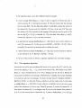
2.1
Selection of the mesh type
The selection of the mesh type depends on the problem to be studied since there is no
strategy that it is considered best for every problem. Among the most common approaches
we mention [8]:
• structured meshes: there is a mapping from the physical space to the computational
space. In the computational space the elements appear as squares (in two dimensions)
or cubes (in three dimensions) and the neighbors and vertices of an element are easily
calculated using an array based data structure. The data structures for this type of
mesh are very regular .
• unstructured meshes: in this case the elements store explicit connectivity information
to determine their neighbors and vertices. The data structures in this case are more
complex than in structured meshes but it is easier to represent complex geometries.
Each type of mesh has its advantages and disadvantages. Structured meshes require
simpler codes with less overhead but are more limited in the representation of complex
domains. Unstructured meshes are more complex, require more storage and overhead per
element but can easily represent complex geometries and moving bodies. Some techniques
implement the meshes as a combination of both approaches. In such cases the mesh is
4
-"
usually decomposed in a set of unstructured super-elements where each super-element is
decomposed into a structured grid.
The choice of the mesh type determines the data structures and algorithms available
for refinement, partitioning and rebalancing. For example, a partitioning method adequate
for unstructured meshes such as Recursive Spectral Bisection [15] is useless for structured
meshes.
A refinement algorithm will perform well on some type of meshes but is not
recommended for anothers. And the migration algorithm described in Section 7.2 highly
depends on how the mesh is actually stored. In the rest of this paper we a.'3sume that the
domain is discretized using unstructured meshes.
2.2
Mesh generation
The generation of meshes for unsteady problems is usually done in two distinct pha.'3es [10]:
• initial mesh creation: involves the creation of a compatible unstructured mesh us
ing the geometry description of the problem domain. The complex topology of the
problem is discretized into a set of simpler elements. This is a global process usually
performed on a sequential computer and it might require human assistance.
• mesh adaptation: the selective refinement/coarsening of sections of the mesh improves
the quality of the solutions either by increasing the resolution in interesting areas or
by decrea.'3ing it on regions of little interest. The refinement of elements is largely a
local process.
The compatibility of the mesh to the problem topology and correct treatment of the
boundaries are not the only requirements for high-quality meshes. In addition it is desirable
to have meshes whose elements are [1]:
• conforming: the intersection of elements is either a common vertex or a common side.
• non-degenerate: the interior angles of the elements are bounded away from zero.
• smooth: the transition between small and big elements is not abrupt.
5
Mesh adaptation
2.3
The following are the two principal strategies for mesh refinement [12J :
• h-refinement: is performed by splitting an element into two or more smaller subele
ments (refinement) or by combining two or more subelements into one element (coars
ening). h is a parameter of the size of the elements. This method involves the modi
fication of the graph structure of the mesh.
• p-refinement: can be thought as increasing the amount of information associated with
a node without changing the geometry of the mesh [10], where p is the polynomial
order of some element.
Through the rest of this paper we concentrate mainly on h-refinement although some
of the techniques for mesh partitioning and migration are independent of the refinement
strategy. Since p-refinement also modifies the workload in each processor the repartitioning
and migration algorithms apply to it also.
2.3.1
Local h-refinement algorithms
Starting from a conforming mesh M formed by a set E of non-overlapping elements E i E E
that discretize a domain
n of interest
and a set of elements R, R
~
E, that are selected
for refinement, h-refinement algorithms construct a new conforming mesh M' of embedded
elements Ei such that:
• if Ei E R, Ei is split into a set of nonoverlapping su belements {Ei t , Ei 2 ,
... ,E:J that replace Ei.
The selection of elements for refinement (or coarsening) in R is made by examining the
values of an "adaptation criteria" [6J that can be related to a discretization error. Usually
these refinement methods cause the propagation of the refinement to other mesh elements so
6
an element Ei
rt R
might also be refined in order to obtain a conforming mesh. Coarsening
algorithms have similar problems.
One common refinement algorithm is the Rivara bisection refinement algorithm for tri
angular elements that it is used in two dimensional problems. In its simplest form it bisects
the longest edge of a triangle to form two new triangles with equal area. There are several
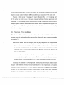
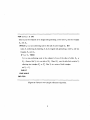
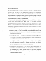
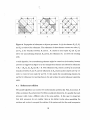
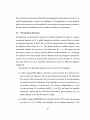
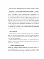
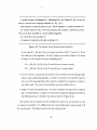
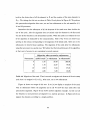
variants of the serial bisection refinement algorithm. In Figure 1 we illustrate an example
of the 2-triangles bisection algorithm [1] and [2] described in Figure 2. In Figure 1 (a)
the element selected for refinement is shaded. The refinement of this element creates a
non-conforming white node on its longest edge. The shaded element in 1 (b) must now be
refined to to maintain a conforming mesh. This process is repeated in (c) where there are
two non-conforming nodes. Finally in (f) we show the resulting mesh. Using the bisection
refinement algorithm the propagation is guaranteed to terminate. Also if we start the refine
ment with a mesh M that ha.'3 elements that are smooth, conforming and non-degenerate
then the elements of the resulting mesh M' will also have the same properties.
3
Multilevel mesh adaptation
To support dynamic adaptation of meshes we designed a data structure based on a multilevel
finite-element mesh with a filiation hierarchy between two consecutive levels. As we will
show in later sections, our algorithms for refinement, partition and migration take good
advantage of this mesh representation.
We a.<;sume that the user supplies an initial coarse mesh M o(E, V) called a O-level mesh
where E is a set of elements and V is a set of nodes. This is the coarsest mesh that the
refinement algorithm is able to manipulate. Using defined adaptation criteria we select
some elements Ei E R
~
E for refinement and others Ej E C
~
E for coarsening.
For each refined element Ei we define the Children(Ei) = {Eill E i2 , .. . , E in } to be the
elements into which Ei is refined and let Parent(Ei,J = Ei. Also for each element Ei E Ewe
define Level(Ei) = 0 if E i is in Mo and Level(Ei) = Level(Parent(Ei))
+ 1 otherwise.
The
children of an element Ei of level l can be further refined and they become the parents of
7
a)
b)
c)
d)
e)
f)
Figure 1: Bisection refinement: in (u) only one element is selected for refinement. (b) shows
the mesh after the refinement of that element. A non-conforming white node is created so
we propagate the refinement to an adjacent element. (c), (d) and (e) show different stages
of the refinement and (1) shows the final mesh. Although only one element was initially in
R we refined 3 more elements to obtain a conforming mesh.
8
FOR each Ei E R DO
bisect Ei by the midpoint of its longest side generating a new node Vp and two triangles
Ei l and Ei 2 '
WHILE Vp is a non-conforming node in the side of some triangle Ej DO
make Ej conforming by bisecting Ej by its longest side generating a node Vq and two
triangles Ejl and Ej2'
IF Vp
# Vq
THEN
Vp is a non-conforming node in the midpoint of one of the sides of either Ejl or
Ei2' Assume that Vp is in one side of Ejl' Bisect E jl over the side that contains Vp
obtaining two triangles Ejl or E~. Now Vp is a vertex of both triangles.
set Vp = Vq .
END IF
END WHILE
END FOR
Figure 2: Rivara's two-triangle refinement algorithm.
9
o
o
o
o
o
o
1
a)
b)
o
o
o
o
.........----- 0
o
3
1
d)
c)
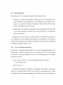
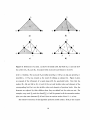
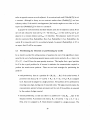
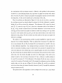
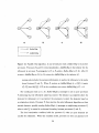
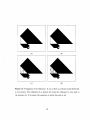
Figure 3: Refinement of a mesh. (a) shows the initial mesh Mo while (b), (c) and (d) show
the meshes M] , M 2 and M 3 • Associated with each node and element is its level.
level 1+ 2 children. For each node Vp we define Level (Vp )
Level(Ei)
+1
if Vp was created
&'3
= 0 if Vp is in Mo and Level (Vp ) =
the result of refining an element Ei. Figure 3 gives
an example of the refinement of a mesh along with the associated levels. Note that the
meshes M I , M 2 and M 3 in (b), (c) and (d) do not only include nodes and elements of the
corresponding level but can also include nodes and elements of previous levels. Also the
elements are replaced by their children when they are refined but the nodes are not. For
example, every node Vp such that Level(Vp )
= 0 will be present in all the successive meshes.
Also note that some elements Ei of level 1 have as vertices nodes of level 1- 1 or less.
The iterative execution of this algorithm produces nested meshes. If M o is the coarsest
10
mesh then for any level l:
where Mi -<
Mi-l
is a relation that indicates that Mi has all the nodes present in
that some elements in
Mi-l
Mi-l
and
have been split to form the elements in Mi.
Multilevel refinement
3.1
A sequence of nested refinements creates an element hierarchy.
In this hierarchy each
element of the initial mesh belongs to the coarse mesh Mo and time t > 0 each element
that it is not refined belongs to the fine mesh.
A decision to perform an n-fold refinement of Ei E R is transmitted to the refinement
module as the pair (Eil n). For example if n
= 1 then using
Rivara's bisection refinement
the element Ei is divided into 2 triangles. If n > 1 then each of its children is refined n - 1
times.
The multilevel algorithm for refinement has the following properties:
• an element that has no parents has level 0 and belongs to the coarse (initial) mesh
Mo. No coarsening is done above this level.
• an element with no children belongs the fine mesh M t . The numerical simulations are
always based on the fine mesh.
• an element could be at the same time in both the coarse mesh M o and the fine mesh
M t (for example before any refinement is done) or in any intermediate mesh.
• only elements that are in the fine mesh M t can be selected for refinement or coarsening.
The hierarchy of elements is only modified at its leaves.
• a node Vp such that Level(Vp ) = l is a vertex of elements Ei of level l or below. An
element Ei of level l has vertices of level m where m
~
1.
• as the elements are individually selected for refinement or coarsening the hierarchy
can have different depths in different regions of the mesh.
11
0-----GJ
a)
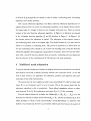
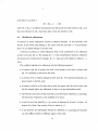
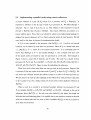
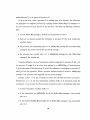
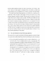
Figure 4: Multilevel refinement.
c)
b)
Initially elements E a and Eb in (a) are selected for
refinement. Both elements are refined and replaced by their children (b). In (c) the element
E a ! is further refined. Under the meshes we show the corresponding mesh hierarchy.
• when an element Ei is refined it is replaced by its children in the fine mesh M t . To
coarsen an element all its children must be selected for coarsening. In this case the
children in the fine mesh M t are replaced by their parent and destroyed .
• both refinement and coarsening can propagate to adjacent elements. The algorithms
are not completely local because they need to preserve conformality requirements.
This sequence of refinements is explained in Figure 4. Initially the elements E a and Eb
are selected for refinement (a). Under the mesh we show the internal representation. Both
E a and Eb belong to M o and M t . After the first refinement 4 new elements are created. At
this point M t includes Ea !, E a2 , Eb! and Eb2 (b).
12
3.2
Local coarsening
The selection of elements for coarsening is performed by evaluating an adaptation criterion
at their vertices. The nodes in a finite element mesh are associated with the degrees of
freedom and the unknowns of a system of equations. After finding its solution at time t the
system might desire the elimination of nodes considered unnecessary according to a selected
evaluation criterion to reduce the number of unknowns. This destruction of nodes requires
coarsening of elements to maintain a conforming mesh.
The successful evaluation of the adaptation criteria at a node Vp is not a sufficient
condition for the destruction of a node.
Nodes created as a result of the propagation
of refinement need to be adequately coarsened to preserve the conformality of the mesh.
Elements at a lower level that reference the node need to be eliminated to prevent dangling
references and this might require the destruction of other nodes. The conditions for a correct
coarsening algorithm are:
• to select an element Ei of level [ as a candidate for coarsening, all its vertices
v;, that
are nodes of level [ should be selected as candidates for coarsening by evaluating the
adaptivity criteria at the node.
• assume that this element Ei of level [ is the child of some other element Ej of level
[-1. In order to replace all the children of Ej by Ej all its children should be selected
&'5
a candidates for coarsening or none of them are.
• a node Vp is selected for coarsening, not anymore as a simple candidate, only if all
its adjacent elements Ei are selected as candidates for coarsening. This condition
prevents dangling references from elements to destroyed nodes.
• if an element E i that is an element of level [ has more than one vertex of level [ and
not all of them are selected for coarsening, then none of its vertices of level [ is selected
for derefinement since an element that has vertices of its level that are not selected
for coarsening will not be coarsened and we need to prevent that its vertices allow the
coarsening of adjacent elements.
13
• finally, an element Ei of level 1 is selected for coarsening if:
the element Ei has no children (it belongs to the fine mesh).
the element Ei has a parent (it does not belong to the coarse mesh).
its vertices are nodes of level m where m
~
1.
all its vertices that are nodes of level 1 are selected for coarsening (and are not
simple candidates). This last condition will ensure that the resulting mesh is
conforming because a node Vp is selected for coarsening only if there will be no
references to it.
4
The challenge of exploiting parallelism
The data structures and algorithms introduced in the previous section allow us to refine
and coarsen a mesh in a serial computer. Most of the work that we will present in the rest
of this paper extends these ideas to a parallel computer. Parallelism introduces a series
of problems that we need to solve in order to perform the dynamic adaptation of parallel
mesh-based computation.
Refinement algorithms typically use a local information to perform refinement. Unfortu
nately the refinement of an element E a that creates a new node Vp in an internal boundary
between two processors requires synchronization between the processors.
The second problem concerns with the termination of the refinement phase. The serial
algorithm terminates when no more elements are marked for refinement. This is not always
easy to detect in a parallel environment. In this case, global refinement termination holds
only when all the processors have refined their elements and there is no propagation message
in the network. A processor P; might have no more local elements to refine but it needs
to wait for possible propagations from neighbor processors. Only when all the processors
agree on the termination of the refinement phase can they proceed to the next phase.
The adaptation of the mesh produces imbalances on the work assigned to each processor
as elements and nodes are dynamically created and destroyed. Also mesh partitions are
14
computed at runtime interleaved with the numerical simulation. In this environment we
cannot afford expensive algorithms that recompute the partitions from scratch after each
refinement. Instead we propose repartitioning algorithms that use the information available
from previous partitions and the refinement history.
Finally we must keep a consistent mesh while migrating elements and nodes between pro
cessors. In our meshes the physical location of nodes and elements is not fixed throughout
the computation. Instead our design supports dynamically changing connectivity infor
mation where the references to remote elements and nodes are updated as new nodes or
elements are created, deleted or moved to a new processor to balance the work load.
In the following sections we address these problems in detail and we present our solutions.
First however, we introduce some definitions, explain a strategy for storing meshes in a
distributed memory parallel computer (that we call a parallel
me.~h)
and show how to use
the mesh to solve dynamic problems.
5
Mesh representation in a parallel computer
In Section 3 we presented a data structure to represent a refined mesh in a serial computer
and we introduced serial refinement and coarsening algorithms. In this section we extend
this data structure to store adapted meshes in parallel computers.
Let M(E, V) be a finite element mesh where E is a set of elements and V is a set
of nodes. We define Adj (Ea )
ElemAdj(Vp )
= {Ea
:
=
{Vp
:
Vp is a vertex of E a }. In a similar way we define
Vp is a node of E a } and NodeAdj(Vp )
= {Vq
:
Vp and Vq are both
nodes of a common element E a }. Adj (Ea ) of an element E a is the set formed by the vertices
of Ea.
In the case of triangular elements IAdj (Ea ) I = 3, and in the case of quadrilateral elements
IAdj (Eb) I = 4.
ElemAdj (Vp ) of a node Vp is the set formed by the elements adjacent
to Vp and NodeAdj (Vp ) is the set formed by the nodes adjacent to Vp • Two nodes are
considered adjacent not only because there is an edge between them in the mesh M but
also if they are adjacent to a common element. In the case of quadrilateral elements two
15
nodes at opposite corners are node adjacent. In an unstructured mesh INodeAdj(Vp ) I is not
a constant. Although in theory we can construct meshes where INodeAdj (Vp ) I can have
arbitrary values, if the mesh is non-degenerate (the interior angles are not close to 0) we
expect that INodeAdj(Vp ) I be close to a constant k.
A graph G is constructed from the finite element mesh M. Its adjacency matrix H ha.<;
one row and column for each node V p E V. The entry hp,q
= 1 if the nodes V p and Vq are
adjacent to a common element and hp,q = 0 otherwise. The adjacency matrix H can be
directly constructed from NodeAdj (Vp). Since V p E NodeAdj (Vq) => V q E NodeAdj (Vp), the
matrix H is symmetric and G is an undirected graph. In general INodeAdj(Vp) I ~
IVI
so
we expect that H will be very sparse.
Partitioning by elements or partitioning by nodes
5.1
In an iterative method for solving systems of equations the cost of the algorithm is domi
nated by the cost of performing repeated sparse matrix-vector products Ab
IVI
X
IVI.
= c where A is
A and H have the same sparsity structure. This implies that a good partition
for G is also a good partition for A because it minimizes the communication required to
perform the matrix-vector products. There are two ba.<;ic strategies for partitioning the
graph G:
• node-partitioning: there is a partition (J? = {(J?l' (J?z, ... , (J?p} of the nodes between P
processors such that
to
~.
U
(J?i
= V and (J?i n (J?j = 0, V i
I- j.
If Vp E (J?i it is assigned
Each node is assigned to a single processor. The partition of G is performed by
removing some edges, leaving sets of connected nodes. The edges removed express the
communication pattern between processors and the cost of the partition is measured
by the number of edges removed .
• element-partitioning: in this case there is a partition II = {Ill, lIz, ... , IIp} of the
elements between P processors such that
If E a E IIi it is a.<;signed
to~.
U
IIi
=E
and IIi n IIj
= 0,
Vi
I-
j.
Each element is assigned to a single processor. The
16
partition is performed across the edges that separate two elements. If Vp E Adj (Ea)
and also Vp E Adj(Eb) where E a E ITi, Eb E ITj and i
i= j
then Vp is a shared node.
Both ~ and Pj have their own copy of Vp , that we will denote V~ and
vl respectively.
Communication is required between multiple copies of the same node so the cost of
the partition is measured by the number of shared nodes.
We define Nodes(ITi) = {V; : E a E ITi and Vp E Adj(Ea)} hence Nodes(ITi) is the set
of nodes corresponding to the elements in ITi. Note that Nodes(ITd
n Nodes(ITj) i= 0
if the two partitions ITi and ITj are adjacent.
To find a partition of the mesh using element-partitioning we first compute the dual
M-l(E,W) of the mesh M where W = {(Ea,Eb): Ea,Eb E E,Ea i= Eb' Adj(Ea)n
Adj(Eb)
i=
0}. W is a set of pairs of adjacent elements so they have at least one
node in common. We then use a graph partitioning algorithm to assign elements to
processors.
It is shown in [13] that partitioning by elements has several advantages over partitioning
by nodes due to the way the matrix A is computed in the finite element method. The matrix
A is the result of an assembly process. We first compute a local square matrix of L(Ea)
(of size IAdj(Ea)l) for each element E a E E. L(Ea) represents the contribution of E a to
its nodes Vp • The global matrix A is equal to
L,EaE E L(Ea) (where L, means the direct
sum of the local matrices after converting from the local indices in L to the global indices
in A). The matrix A is also partitioned between the processors. If the node Vp is a shared
node between two or more processors Pi and Pj then the entry in Ai corresponding to V~
has the contributions of the elements E a E ITi and the entry in Aj corresponding to
V;
has the contributions of the elements Eb E ITj. The matrix Ai in processor Pi is partially
assembled since it only considers the contributions of the elements E a E Pi. The fully
assembled matrix is A = L, Ai .
The matrix-vector product Ab =
C
is performed in two phases. In the first phase each
processor computes Aib = Ci. The resulting vectors Ci are also partially assembled. In the
second phase we communicate the individual vectors Ci to obtain C=
17
L, Ci.
Implementing a parallel mesh using remote references
5.2
A remote reference is a pair (~, V~) where Pi is a processor and V~ E Nodes (TIi)' It
represents a reference to the V~ copy of node Vp in processor Pi. We define Ref(V~)
{(Pj, VJ) : VJ is a copy of Vp in Pj, i
t=
=
j}. This relation is also symmetric so that if
(Pj, vj) E Ref(V~) then (Pi, V~) E Ref(Vj).
The remote references are pointers to a
remote address space. Since this is not allowed in almost any programming language we
designed the remote references as C++ objects using the notion of smart pointers. We will
come back to this when we discuss the implementation details.
If Vp is a node internal to the processor, then Ref(Vp )
= 0.
A node in an internal
boundary can be shared by more than two processors. Hence if Vp is a shared node then
1 :::; IRef(Vp ) I
:::;
P - 1 where P is the number of processors. In a conforming mesh we
expect that IRef (Vp ) I
~
P - 1 and usually IRef (Vp ) I = 1 for a shared node since most
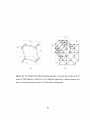
of the shared nodes are shared by only two processors in a 2-D mesh. The example in
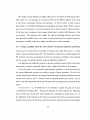
Figure 5 shows a mesh with 8 elements and 9 nodes.
processors Po, PI, P2 and P3 so Ref(V".p)
The node V4 is shared by four
= {(PI, Vl), (P2 , V1), (P3, Vln
while Ref(Vl)
{(Po, 'v.p), (P2 , vi), (P3, vln. Figure 6 states for initializing the references.
There is no need to have more than one copy per node in each processor. Suppose that
a processor ~ has two copies of the same node V; and V~' so that (~, V/) E Ref(V~). We
can detect this condition because the reference points to a node in the same processor Pi.
We then remove the copy
to
V/
V/ after updating all the references in other processors that point
to point to V~. For a similar reason we do not need or allow duplicate references in
Ref(V;).
When a node Vp is created in an internal boundary between two processors
~
and
Pj we initialize Rej(V~) = {(Pj, vjn and Ref(Vj) = {(Pi, V~)}. Although at the end of
refinement phase IRej(V~) I = 1 for each new node created in that phase, this might not
hold after the load-balancing phase. It is possible that a new partition converts an internal
node into a shared node and vice versa or that it modifies Rej(V;) so that it is shared by
more than two processors.
18
PO
................................. .:
.
P3 :
.........................
.
..........................
a)
b)
Figure 5: A square mesh partitioned by elements between four processors (a) and its
internal representation using remote references (b).
19
INPUT: M(E, V) where M is a finite element mesh with a set E of elements and a set V
of vertices.
-
compute the dual M- 1 (E, W) of M where W = HE a , Eb) : E a , Eb E E, a =/:- b,
Adj(Ea ) n Adj(Eb) =/:- 0}. W is a set of adjacent elements and Adj(Ea ) is the nodes
of element Ea.
- partition M- 1 into P regions using a graph partitioning algorithm such that E a E lli if
E a is assigned to
F'i
where
U lli = E
and lli
n llj
=0
Vi=/:- j.
- Nodes(ll;) is the set of nodes corresponding to elements in lli. Note that is not required
that Nodes(lli)
n Nodes(llj) =/:-0.
FOR each V~ E Nodes(lli) in parallel DO
Ref(V~)
= 0
END FOR
FOR each V~ E Nodes(ll;) in parallel DO
IF E a E ElemAdj(Vp ) and E a E llj and j =/:- i THEN
Ref(V~) = Ref(V~) U (Pj,
vt)
END IF
END FOR
Figure 6: Computing the initial references in a parallel mesh.
20
The design of these references is highly influenced by the element partitioning method.
Their main use is to maintain the connections between the different regions of the mesh
as the mesh is partitioned between the processors. As will be shown in later sections,
they provide a very flexible mechanism for maintaining a dynamic mesh. When a node is
moved to a new processor it can use its reference list to find its copies in other processors.
It can then send a message to these copies telling them to update their references to the
new location. The references also simplify the task of assembling matrices and vectors
from partially assembled ones as new nodes are created and moved at runtime because no
assumption is initially made about origin and destination of these messages.
5.3
Using a parallel mesh for the solution of dynamic physical problems
In this paper we assume that we are given an initial coarse mesh M o at time t
which we find an initial partition
nO.
= 0 from
This partition is computed in a preprocessing step.
We distribute the nodes and elements between the processors according to that partition
and we compute the initial references using the algorithm in Figure 6.
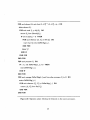
Our algorithm for finding the solution of dynamic problems consists of four consecutive
phases that we execute repeatedly. Figure 7 gives a high level outline of the program.
In the first pha.se we use numerical approximation techniques to find the solution of
the partial differential equations by solving a system of linear equations. We solve this
system using iterative methods. As we have mentioned earlier we generally perform repeated
matrix-vector products Ab
= c when
we need to assemble matrices and vectors. All the
effort in the following phases has the goal of improving the performance and quality of this
pha.se.
At some time t
= tk
we decide that it is convenient to adapt the mesh so we start
a refinement/coarsening pha.se. Using error estimates we select elements for refinement
that we insert into R and if we select elements for coarsening we insert them in C. If
the refinement of the elements in R creates a new shared node Vp in an internal boundary
between two processors Pi and Pj we create the two local copies V; and V/ and we initialize
21
- find an initial partition Ilo.
- load the mesh using the partition Ilo.
- initialize the references Ref (V;) using the algorithm in Figure 6.
FOR t < T DO
- compute a solution.
- refine/coarsen the mesh. For each new shared node V; determine Ref(V;).
- find a new partition Il t .
- migrate the elements and nodes according to Ilt. If a node V; is moved from ~ to P j
then if Vpk is another copy of Vp in Pk update Ref(V;) = ((Ref(V;) - (Pi, V;)) U (Pj , vj)
and set Ref(Vj) = Ref(V;).
END FOR
Figure 7: Outline of a general algorithm for computing the solution of dynamic physical
system using a paralle.! mesh.
Since adaptation produces imbalances in the distribution of the work, we compute a
new partition Il t • If Il t
=1= Il t -
1
we need to migrate some elements and nodes to adequate
the mesh to the new partition. This phase does not create new nodes or elements but it
modifies the reference lists as nodes are moved to new processors.
6
Parallel mesh adaptation
Using the data structures presented in the previous section we now introduce an algorithm
for adapting the mesh in a parallel computer. Let R be a set of elements selected for
refinement and let Ri be the subset of the elements of R assigned to processor
case R
= URi
and also Ri n Rj
=0
for i
=1=
~.
In this
j because by using the element-partitioning
method of assigning elements to processors each element is assigned to only one processor.
Each processor has all the information it needs to refine in parallel its own subset Ri using
22
a)
b)
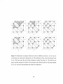
c)
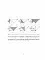
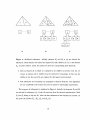
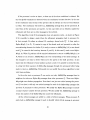
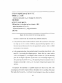
Figure 8: Propagation of refinement to adjacent processors. In (a) the elements E a , E e , Ej
and E g are selected for refinement. The refinement of these elements creates two nodes, Vp
and Vq , in the boundary between Po and Pl. PI creates its local copies Vi and Vql and
selects the nonconforming elements Eb and Eh for refinement (b). (c) shows the resulting
mesh.
a serial algorithm, but nonconforming elements might be created on the boundary between
processor as suggested in Figure 8. In that example four elements are selected for refinement
so R o = {E a , E e , Ej, E g } and R 1
= 0.
The refinement of E a creates a node V~ in an internal
boundary between Po and PI and the refinement of E g creates another shared node ~o. PI
needs to create its local copies Vp1 and Vi. It then marks the nonconforming elements Eb
and Eit for refinement by inserting them in R I and invokes the serial refinement algorithm
again.
6.1
Refinement collision
The parallel algorithm can run into two synchronization problems [3]. First, if processor Pi
refines an element E a and processor Pj refines an adjacent element E b , it is possible that each
processor could create a different node at the same position. In this case it is important
that both processors do not consider them as two distinct nodes when assembling the
matrices and vectors to compute the solution of the system and that the node incorporates
23
the contributions of all the elements around it. Related to this problem is what processor
~
believes is a nonconforming element Eb in processor Pj might have already been refined
there. Processor Pj needs to evaluate and update the propagation requests it receives before
executing them. In this case Pj should insert a descendant of Eb in Rj.
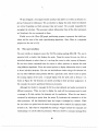
These two problems are illustrated in Figure 9. In the top row we show a case where
the receiving processor has already refined the element but further refinement is required.
Initially E a and Eb are selected for refinement. The refinement of E a creates the shared
node Vpo. PI creates its copy of Vp but it then has to determine which of the children of
Eb (Eb 1 or Eb2) should be inserted into R I for further refinement. In the bottom row the
receiving processor should only update the reference rather than creating a new copy. Both
Po and PI create shared nodes (Vp and Vq ) in the same mesh location as the result of the
refinement of E a and Eb. We need to detect that both nodes are the same and update the
references accordingly.
The solution to the synchronization problem is greatly simplified by using the nested
elements of our multilevel algorithm. When an element Eb in processor Pj is refined into
two or more elements Eb l and
E~
the element Eb is not destroyed as it would be the case
in other refinement algorithms. Any message arriving to processor Pj from processor
~
with the instruction of making a copy of a shared node Vp in processor Pj (named VJ) that
causes the refinement of the element Eb can be compared against the status of the element
Eb. If the element Eb was already refined in the local phase (but processor
~
did not know
about this), then the element Eb might not need to be refined again. If the node Vp was
already created in the local phase of processor Pj then a reference is added pointing to
its copy
V; in processor ~. If the refinement of the element Eb did not cause or was not
caused by the creation of the shared node Vp (for example the refinement was done dividing
another edge
as
in the top row of Figure 9), then its children Ebl and Eb2 are evaluated
and the one that shares the internal boundary between Pi and Pj is marked for refinement
using the shared node
V,t.
The pseudocode for this algorithm is shown in Figure 10 but there are a some details
24
................................................... :
:
:
....................................................
a)
c)
h)
.
--
PI,
PO
. PO
:
:
a)
: PO
:
:
h)
:
:
c)
Figure 9: Refinement of adjacent elements located in different processors. In the top row
two elements are selected for refinement (a). The refinement of E a creates the shared node
Vp (b). We then select Eb1 for further refinement (rather than Eb) (c). The bottom row
shows another example (a) where two processors create shared nodes in the same position
(b). In (c) we detect this problem and update the references.
25
Ri is the set of elements selected for refinement in Pi.
WHILE Ri /; 0
DO
- extract an element E a from Ri.
- refine E a using a serial refinement algorithm.
FOR each shared node
V; created in an internal boundary between F'i and Pj
Send a message from Pi to Pi requesting the creation of a shared node
node
v,1
v,1
DO
in Pi' If a
already exists, then return a reference to it. Otherwise, create the node
vj,
determine the element to refine, and insert it into Ri' Finally return its reference to Pi.
END FOR
END WHILE
Figure 10: Avoiding refinement collisions in a parallel mesh.
that they are not explained there. First, we do not send a message for each individual node
because of the high cost of sending messages. Instead we first refine all the elements in
Ri keeping track of the shared nodes that Pi creates as a result of refining elements in Ri.
Once Ri
= 0, Pi sends the messages to its adjacent processors and listens for
propagation
messages from them. If it receives such a message it creates the new shared nodes and
inserts the nonconforming elements into Ri.
To determine which element to refine we use ElemAdj (Vp ). Suppose that the refinement
of an element E a in Pi creates a shared node Vp in a boundary between F'i and Pi' This
new node is created at a midpoint between two other shared nodes Vq and Vr • Note that
(Pi, vj) E Re!(V:) and also (Pi, Vi) E Re!(Vj). We use these references to send a message
from F'i to Pi' When Pi receives this message, it determines the unrefined element Eb E
ElemAdj (vj)
n ElemAdj (VI) and inserts it into Ri'
As it can be easily seen, the parallel algorithm is not a perfect parallelization of the
serial one and it can result in a different mesh. The serial Rivara's algorithm [1] and [2] first
selects an element E a from R. It then continues refining all the nonconforming elements
26
that result from the refinement of E a before proceeding with another element from R. In our
parallel implementation we ignore this serialization. We approximate the serial algorithm
within each processor as much as possible but do not impose it across processor boundaries.
We claim that this modification does not affect the quality of the refinement.
6.2
Termination detection
The algorithm for detecting the termination of parallel refinement is based on a general
termination algorithm in [4]. A global termination condition is reached when no element
is marked for refinement, so if R is the set of all the elements selected for refinement, then
the algorithm finishes when R
=
0.
termination condition for processor
Pi
This global termination condition implies a local
that holds when Ri = 0. We assume that the
refinement is started in one special processor referred to as the coordinator, Pc. To simplify
the explanation we assume initially that the refinement does not propagate cyclically from
processor Pi to processor Pi and then from processor Pi back to processor Pi. We will
show later that this is not a reasonable restriction but it does not affect the algorithm
significantly.
The algorithm for detecting termination uses two basic kind of messages:
• a refine message Refine-Msg( i, j) sent from a source processor Pi to processor Pi is
used to request the refinement of one or more elements of processor Pi' We will specify
the contents of this message later but let's assume for now that it can either indicate
the elements selected for refinement (if the message is sent by the coordinator) or it
can include a reference to a shared node. If Pi receives a Refine-Msg(i,j) = {V;}
it creates the node
vt, it initializes Rej(Vt) =
{(Pi, V;)} and inserts the unrefined
element E a E Adj(Vp ) into Ri' Note that at this stage V; has no reference to V{ To
update Ref(V;) we use the next type of message.
• an update message AddRej-Msg(j, i) is returned from Pi to Pi for each refine message
sent from Pi to Pi to indicate the completion of the requested refinement. This
27
a)
c)
b)
----:~~
d)
Refine-Msg
- - - - - -> AddRef-Msg
Figure 11: Parallel refine algorithm. In (a) the initiator sends a Refine-Msg to each other
processors. Processors Po and P j return immediately a AddRej-Msg to the initiator but the
refinement in processor P 2 propagates to P j so P 2 sends a Refine-Msg to P j (b). After P j
returns a AddRej-Msg to P2 (c), P z returns its AddRej-Msg to the initiator (d).
message also includes the necessary information to update the references to the nodes
shared between Pi and Pi' When Pi receives an AddRej-Msg(j, i) = {VJ} it inserts
(Pi, VJ) into Rej(V;). If Pi is the coordinator we return AddRej-Msg(j, C) = 0.
The coordinator sends at t = 0 a Refine-Msg(C, i) message to one or more processors
Pi indicating that the refinement phase has started. The initiator can explicitly select the
elements for refinement or it can instruct the processors to select the elements based on
an adaptation criteria. Processor Pi then executes the serial refinement algorithm on these
marked elements, possibly sending Refine-Msg( i, j) messages to neighboring processors Pi
when a node
V; is created in an internal boundary between processors Pi and Pi'
The local termination condition holds for processor Pi when no more elements are
marked for refinement. When this condition holds, processor Pi does not generate new
28
_lP_
Refine-Msg messages and it is not
waitin~
for any AddRef-Msg messages. Also proces
sor Pi does not insert new elements into Ri until a Refine-Msg(j, i) message arrives from
some other processor Pj. In this case, new nodes are created in the internal boundary as
instructed in the message and the corresponding elements are selected for refinement by
inserting them into Ri. Then processor Pi executes the serial refinement algorithm, which
might cause further propagation to other processors. An example is shown in Figure 11
where Pc sends an initial Refine-Msg to the other processors. Po and PI complete their
work without propagation so they return a AddRef-Msg message to Pc. On the other hand
the refinement of elements in P 2 propagates to PI so P2 sends a Refine-Msg(2, 1) message
to Pl' PI completes this request without further propagation so it returns to P2 which in
turn returns an AddRef-Msg(2, C) message to Pc.
We say that the parallel refinement terminates (the global termination condition holds)
at some t if:
• Ri
=0
for each processor Pi at time t .
• there is no Refine-Msg or AddRef-Msg in transit at time t.
The termination detection procedure is based on message acknowledgments. In particu
lar Refine-Msg(i,j) messages received by processor Pj from processor Pi are acknowledged
by Pj by sending to Pi a AddRef-Msg(j, i) message. These messages return the references
to the newly created vertices so that if v~ is a vertex in processor P;, over a shared edge
that caused a propagation to processor Pj and
vj
is its copy in processor Pj, a reference to
v~ is added at v~ and vice versa.
A processor P;, can be in two possible states: the inactive state and the active state.
While in an inactive state Pi can send no Refine-Msg or AddRef-Msg but it can receive
messages. If it receives a receives a Refine-Msg(j, i) from another processor Pj while in an
inactive state it moves from the inactive to the active state. It creates the shared nodes
as stated in the message and proceeds to refine the nonconforming elements. The message
Refine-Msg (j, i) is called the critical message because it caused the refinement that Pi is
29
performing and P j is the parent of processor Pi.
In the active state, while a processor Pi is refining some of its elements, the refinement
can propagate to a neighbor processor P k requiring another Refine-Msg(i, k) message to it.
An active processor becomes inactive at the first time t for which the following conditions
hold:
• no new Refine-Msg message is received by the processor at time t.
• there are no elements marked for refinement in processor Pi (the local termination
condition holds).
• the processor has transmitted prior to t an AddRef-Msg message for each Refine-Msg
message it has received except for the critical message.
• the processor has received prior to t a AddRef-Msg message for each Refine-Msg
message it ha.<; transmitted.
Using this definition, the local termination condition might hold in processor P;. (Ri = 0)
but processor P;. might be in an active state waiting for a AddRef-Msg(j, i) from processor
Pj if the refinement of the elements of P;. caused the refinement to propagate to processor Pj
and P:J. ha.<; not yet responded. When a processor becomes inactive it returns a AddRef-Msg
message to the processor that originally sent its critical message.
Initially, at time t = 0, the coordinator is active and all other processors are inactive.
Furthermore, at t = 0, the local termination condition holds at all processors except the
coordinator. It can be seen that if a processor is inactive at time t, the following rules hold:
• its local termination condition holds at t.
• it ha.<; transmitted an AddRef-Msg for all the Refine-Msg messages it ha.<; received
prior to t.
• it ha.<; received AddRef-Msg messages for all Refine-Msg messages it has transmitted
prior to t.
30
If the processor is active at time t, at least one of the above conditions is violated. We
say that global termination is detected when the coordinator becomes inactive. In the ca.'3e
of the coordinator only the last of the previous rules is relevant as it has no local elements
to refine. The coordinator will receive an AddRef-Msg message from all the processors Pi
only when all the processors are inactive. In this case there are no elements marked for
refinement and there are no other messages in the network.
This algorithm works if the propagation does not generate cycles. As shown in Figure
12 it is possible to design a mesh where the refinement propagates back to processor Po.
In that example Po refines an element E a creating a shared node Vpo. It then sends a
Refine-Msg(O, 1) to PI' PI creates its copy of the shared node and proceeds to refine the
nonconforming elements but before PI is ready to return a AddRef-Msg(l, 0) a new shared
node ~I is created in the boundary between PI and Po. In this case PI sends a new Refine
Msg(l, 0). When Po performs all the required refinements it returns a AddRef-Msg(O, 1) to
PI which in turn returns a AddRef-Msg(l, 0) to Po corresponding to the initial message. In
this example is not easy to detect which one is the parent or the child processor. It also
shows that the refinement of some meshes can have a cycle. It is possible to extend the idea
to a long but finite sequence of Refine-Msg messages through two processors before being
ready to return a AddRef-Msg. Fortunately we can modify the previous algorithm to deal
with these problems.
In the active state a processor Pi can receive not only AddRef-Msg messages from its
neighbors but also new Refine-Msg messages from other processors Pj. These new Refine
Msg might cause further propagation. Now there is not just one critical message for proces
sor
~
but there is still only one critical message for each of the Refine-Msg messages that
processor Pi transmits to other processors. We modify the Refine-Msg message to include
a unique sequence number for each processor. We also modify the AddRef-Msg message to
return the number of the Refine-Msg that caused the refinement.
All the critical messages are added to a table of critical messages. When processor Pj
sends back a AddRef-Msg message it needs to identify which critical message in processor
31
':
'"
~.'
............................................. : :
.
:
~
: :
~
ro
n
::
··:
.:
PO
·:
··: :..
·· ..
··· ...
·· ..
·· ..
~ ~
.
·.
·
:;
"::::
.'
........................ :
:
.
.L-..----------c.p~
..._---.
: : p
~
b)
~
:"
*
.........................................................................
:
a)
~
~
\
~----<
PI
·: :.
"'---------.
-M- ...---~.
)<
·.
.
"
~
ro
.'
: :
n
PO
PI
.---.
~ .~
,
....---I.~
·.
:~
--H- ...--....--<.
~
~
.....
.L-..
~.
~
~
.
:
-
~. ~
c)
:
..._-....- .
~.
.
d)
Figure 12: A propagation cycle. Po has initially one element marked for refinement (a).
The refinement propagates to PI (b) and then comes back to Po (c). (d) shows the final
mesh.
32
FOR each processor
~
DO
send Refine-Msg(C, i) indicating elements to refine.
END FOR
FOR each processor
~
DO
wait for an AddRef-Msg(i, C).
END FOR
FOR each processor
~
DO
send Con tin ue-Msg (C, i) to finish the refinement phase.
END FOR
Figure 13: Detecting the termination of the refinement phase (Coordinator algorithm).
~
caused the propagation to Pj using the sequence number. When a critical message
in a processor Pi receives a AddRef-Msg message for all the propagations it caused, then
processor
~
removes the critical message from the table and it sends back a AddRef-Msg
message to the processor that initially sent that critical message to it. The processor
~
is
in the inactive state if Ri = 0 and it has no critical messages in its table. The pseudocode
for the algorithm executed by the coordinator is shown Figure 13 while Figure 14 has
an outline of the program executed by all the remaining processors. This pseudocode is
explained below.
Initially Pc sends a Refine-Msg(C, i) to all the other processors ~ to start the refinement
phase. These messages are used to select the elements in Ri to be refined in
~.
Each
~
returns a AddRef-Msg(i, C) once they have refined these elements and has also received a
AddRef-Msg(k, i) for each Refine-Msg(i, k) produced by the propagation of the refinement
to
~.
The algorithm uses a new type of message:
• a continue message Continue-Msg( i, j) sent from the initiator to every other processor
is used to inform them that the refinement phase concluded and that they can continue
to the next phase.
33
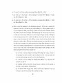
seq
=0
WHILE true DO
wait for a message msg.
IF msg = Continue-Msg(j, i) THEN
return.
ELSE IF msg = Refine-Msg(j, i) THEN
set seq++, table[seq].critical = msg and table[seq].count = 0
FOR each element E a E msg DO
create the shared nodes and insert E a in Ri.
END FOR
refine the elements in Ri
FOR each shared node V; created in an internal boundary between P;. and Pk DO
send Refine-Msg( i, k) containing seq and the elements to refine.
table[seq].count++
END FOR
IF table[seq].count = 0 THEN
return AddRef-Msg( i, j) as msg did not cause refinement to other processors.
END IF
ELSE IF msg
= AddRef-Msg(j, i)
THEN
seq is the sequence number returned by msg. set table[seq].count -
IF table[seq].count = 0 THEN
send AddRef-Msg( i, j) to Pj where Pj sent the message stored in table[seq].critical.
END IF
END IF
END WHILE
Figure 14: Detecting the termination of the refinement phase.
34
Once Pc has received a AddRef-Msg from each other processor it broadcasts a Continue
Msg.
Each processor Pi starts the refinement phase waiting for a message. If it receives a
Continue-M.'1g from the initiator it knows that it can proceed to the next phase. If the
message is a Refine-Msg(k, i) it inserts the elements indicated in the message in Ri and
refines it using the serial algorithm. Rather than having one critical message now Pi can
have several critical messages sent by the same or different processors. P; gives them a
sequence number and stores them in a table. If the refinement of the elements in Ri creates
shared nodes in a boundary between Pi and Pj then Pi sends a Refine-Msg( i, j) message to
Pj' Pi keeps track of how many of these Refine-Msg(i, j) it sends for each critical Refine-Msg
it receives. Once it ha.<; received a AddRef-Msg(j, i) for each Refine-Msg(i,j) it can send
back a AddRef-Msg(i, k) response to Pk. Pi continues to listen for messages until it receives
a Continue-Msg from the coordinator. Figure 15 shows an example where the refinement
propagates cyclically between processors.
7
Load balancing
In this section we present a strategy for repartitioning and rebalancing the mesh. We first
explain serial multilevel refinement algorithms. We then introduce a new highly parallel
repartitioning method called the Parallel Nested Repartitioning (PNR) algorithm which is
fa.<;t and gives high quality partitions.
In Section 7.2 we explain a mesh migration algorithm. This algorithm receives as input
the partition obtained from the repartitioning of the mesh and migrates the elements and
nodes according to this partition.
7.1
The mesh repartitioning problem
While the PNR repartitioning algorithm is based on the serial multilevel algorithms pre
sented in [15], [20] and [18] it also makes use of the refinement history to achieve great
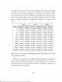
reductions in execution time and an improvement in the quality of the partitions produced.
35
(a)
(b)
(c)
(d)
Figure 15: Propagation of the refinement. In (a) we show an arbitrary mesh distributed
in 4 processors. The refinement of an element (b) causes the refinement to come back to
the processor (c). If we repeat this operation we obtain the mesh in (d).
36
General multilevel algorithms partition the mesh by constructing a tree of vertices. They
create a sequence of smaller graphs by collapsing vertices, then partition a suitable small
graph and finally reverse the collapsing process to produce a partition of the larger graphs.
The Parallel Nested Repartitioning algorithm can be divided into a serial phase and a
parallel phase. When the graph is small enough to fit into one processor we use a serial
refinement algorithm to partition the graph. When the mesh is very large as in the case of
a highly refined mesh we collapse vertices in parallel. The PNR method differs from other
methods in that it uses the refinement history of the mesh to collapse the vertices while
other methods use maximum matchings or independent sets. As a consequence we are able
to collapse vertices locally in the parallel pha.'3e without any communication overhead unlike
other methods. Our tests show that by using the refinement history we obtain partitions
that are almost always of higher quality than those obtained by the multilevel algorithms
yet PNR is very fast. For simplicity we assume that the initial mesh fits into one processor
and marks the transition between the serial and the parallel pha.'3e. In Section 7.1.5 we
discuss possible generalizations of this method.
7.1.1
The serial Multilevel Graph Partitioning algorithms
The pseudocode for a standard serial Multilevel Partitioning Algorithm is sketched in Figure
16. III general serial multilevel algorithms perform the partitioning of a mesh in three phases:
• in the coarsening phase these algorithms construct a sequence of graphs Go, G I , .. . Gk
such that the
IGil < IGi-II
by collapsing adjacent nodes or contracting edges. This
contraction is implementing by finding a maximal independent set [16] or a maximal
matching [20]. Given a graph G(V, F) where V is a set of vertices and F is a set of
edges then V' ~ V is an independent set of G if for all v E V', (v, w) E F
=}
w
~
V'.
An independent set Viis maximal if the the addition of any vertex in V' would make
it no longer an independent set. A matching of G is a set F '
~
F od edges such
that no two of which are incident on the same verex. A mathing F ' is maximal if
the addition of an edge in F ' would make it no longer a matching. A contraction
37
compute the weighted graph Mol (E, W) = Go.
WHILE
IGil > K
DO
compute a coarser graph Gi+l by collapsing the vertices of Gi.
END WHILE
partition the coarsest graph Gk.
FOR each level i in the refine tree from k downto 0 DO
project the partition of Gi to Gi-l.
improve the partition of Gi-l using local heuristics.
END FOR
Figure 16: Serial Multilevel Partitioning algorithm.
IGil is smaller than
operation is repeated until
a defined constant K .
• in the partitioning phase standard multilevel methods find a partition II of the graph
Gk using anyone of a number of different graph partitioning algorithms such as
Recursive Spectral Bisection [15]. Note that typically
IGkl
~
IGol so their use of RSB
is generally not very expensive.
• in the uncoarsening phase these methods project the partition found for G i to the
graph G i -
l
by reversing the collapsing process. Assume that two or more vertices
v and w in the graph
Gi-l
are collapsed to form a vertex u in Gi in the coarsening
phase. If u is assigned to processor Pq then both rand s are initially assigned to Pq .
After projecting the partition to
Kernighan and Lin [32] on each
Gi-l,
Gi-l
they typically perform local heuristics such as
for the purpose of improving the quality of the
partition.
To implement this algorithm on a parallel computer note that for each level of the
coarsening phase we need to compute either an independent set or a matching of the graph.
This implies that for each
Gi-l
we will need to send messages to insure that two adjacent
38
processors do not select adjacent vertices of the graph at the same time, an operation that
can be very time consuming. As we will show, our algorithm uses a different heuristic for
collapsing the vertices of the graph that does not require synchronization at each level.
1.1.2
General repartitioning of an adapted mesh
In Section 5.1 we explained that our meshes are partitioned by elements. That is, given
a mesh M(E, V) where E is a set of elements and V is a set of vertices we construct a
partition IT = {IT I , IT 2 , ••• , ITp} such that each element E a E E is assigned to only one
partition ITi. This is done by creating a graph M- 1 (E, W) that is the dual of M where W
is a set of pairs of adjacent elements: (Ea , Eb) E W if and only if E a and Eb are adjacent.
Thus the elements in E are the vertices of the graph M- 1 and the pairs in Ware its edges.
A partition of the vertices of M-l is a partition of the elements of the mesh M.
In order to contract the graph while preserving its global structure we associate weights
to each element E a and each pair of adjacent elements (E a , Eb)' Given the graph M- 1 we
define Elem Weight (Ea ) to be the number of descendants of E a in the fine mesh (or 1 if E a
has no children). We also define EdgeWeight(Ea ) to be the number of edges between the
descendants of E a in the fine mesh. That is Edge Weight (E a )
= LtEb,EcEM (Eb, E e )
t
such
that Eb and E e are the lowest level descendants of E a and they are adjacent to each other.
For each pair (Ea , Eb) E W we define Weight(Ea , Eb) to be the number of edges between
the descendants of E a and Eb in the fine mesh. Note that if both E a and Eb are unrefined
then Weight(E a , Eb) = 1.
Although we defined Elem Weight, Edge Weight and Weight based on our multilevel
elements of Section 3 we could also define· them recursively for any mesh. Given a graph
M-l (E, W) we can define ElemWeight(Ea ) = 1, EdgeWeight(Ea ) = 0 and Weight(Ea , Eb) =
1 if E a and Eb are adjacent and 0 otherwise. If we collapse two or more elements E a and
Eb into one element E e then:
Elem Weight(E e ) = Elem Weight(Ea )
Edge Weight(Ee ) = Edge Weight(Ea )
+ Elem Weight(Eb)
+ Edge Weight(Eb) + Weight(Ea , Eb)
39
In a similar way we can define Weight(Ec • Ed) for two collapsed elements E c and Ed.
The goal of the coarsening phase in the partitioning algorithm is to approximate cliques.
A refined vertex E a of the graph M- I approximates a clique if EdgeDensity(Ea) = (2x
EdgeWeight(Ea))j( EdgeWeight(EaH EdgeWeight(Ea) - 1)) is close to 1 and it does not
approximate a clique if it is close to O. Intuitively, if a vertex E a has a a large edge density
it will not be cut in half by the bisection in the partition of the contracted graph.
7.1.3
The Parallel Nested Repartitioning (PNR) algorithm
The partitioning algorithm that we discuss in this section incorporates the idea that the
fine mesh M t at time t was obtained as a sequence of refinements of a coarse initial mesh
Mo. The mesh M t includes all the elements E a such that Children(Ma) =
(0
at time t.
IMI as the number of elements in the mesh. We assume that IMol < IMt I but in
IMol ~ IMtl. Note that it is possible to have an element E a E M o n M t if E a is not
We define
general
refined.
Figure 17 shows an example of an initial mesh M o and the refined mesh M t at time
t. The amount of work for processor Po is far larger than the amount of work of the
other processors. The goal of the repartitioning algorithm is to rebalance the work so each
processor has approximately the same number of elements.
The PNR algorithm uses the information that M t was obtained as a sequence of refine
ments. Rather than computing directly a partition of M t it computes a partition of M o
and then projects this partition to M t . The notion is that in the coarsening phase we do
not need to find a matching or independent set to collapse the children of refined elements.
Instead we use the refinement tree to collapse the descendants of each element of the coarse
mesh Mo. In Section 9.6 we compare the PNR with the serial multilevel algorithm. By
using the refinement history we are able to obtain better partitions at a lower cost than the
standard methods.
Our PNR algorithm allows for a very natural parallel implementation. Is is possible
to compute the Elem Weight, Edge Weight and Weight of MOl in parallel using only local
40
ro
~-TI---~
PO
PI
~_._-~~
......__ L_._ __
I
J~J
I ' ,
i~t
I
I
1
~~--_~
.
Pl
:--~
... __ .. J.J.. J ...... J~J ~~.L .....L ..... .+. .......
, ~f+-~H
P2
...
:--~
...:_-+
_ .+.
•••.•••.• ~ .•••••.••••.••.•• .I••.• ~", .••. I••••.••••..••.•••• J••••••••
.................................
...
~-:--r-~
........!
P2
P3
I
I
I ' ,
I
I
!
.
mJ:tm
•
12=SL-~~
PI
............................
.
I
1•••• ~ •••••••••1•••• / " , •••• 1••••••••• t
.
.
b)
a)
Figure 17: The Parallel Nested Repartitioning algorithm. (a) shows the initial mesh M o
and (b) shows the mesh M t at the beginning of the partitioning phase.
information. We then send the graph MOl to a common processor Pp which partitions
the reduced graph M O- 1 • At this point all the other processors wait until Pp sends back a
message informing them of which elements to migrate. Finally, the migration is performed
by moving fully refined subtrees. The partitioning algorithm will inform a processor Pi of
the elements E a E M o to move to another processor Pj. It is assumed that P; will not only
send E a but also all its descendants to Pj. The intention is not to break partition trees to
simplify the unrefinement of the elements. In the rest of this section we will explain the
algorithm in more detail using the example shown in Figure 17. The pseudocode for the
PNR algorithm is shown in Figure 18 and explained below.
As we explained earlier, our Parallel Nested Repartitioning algorithm for mesh parti
tioning can be divided into a parallel phase and a serial phase:
• we construct in parallel the weighted graph Mol. Communication is not required at
this point. Each processor P; computes the weights of each element E a E Mo. This
is done using a simple recursive algorithm. In the same way it computes the weight
41
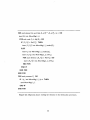
- in parallel compute ElemWeight (Ea ) , EdgeWeight(Ea ) and Weight(Ea , Eb) for each ele
ment E a and each pair of adjacent elements (Eal Eb) E Mol.
- each processor ~ sends its portion of Mol and the weights to a common processor Pp.
- Pp receives sections of M O- I from each processor and computes a partition II of M o- 1 .
This can be done using RSB or a serial multilevel algorithm.
- Pp returns II to each processor Pi.
- Pi migrates the elements and nodes according to II.
Figure 18: The parallel Nested Repartitioning algorithm.
of each edge W
= (Ea , Eb).
Once Pi obtains its portion of Mol it sends it to Pp for
the serial part of the algorithm. The Mol graph for the mesh in Figure 17 is shown
in Figure 19. We consider two ways of defining set W:
- W = {(Ea , Eb) : E a , Eb E Mo, E a and Eb have a common vertex}.
W = {(Ea , Eb) : E a , Eb E Mo, E a and Eb have a common edge} .
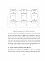
• once Pp receives a message for each processor Pi it partitions the reduced graph MOl
using a serial partitioning algorithm. As IMol1 is a.'3sumed to be relatively small we
can use at this stage algorithms that would be considered too expensive to apply to
the refined mesh. The result of this partition is shown in Figure 20 (a).
• finally we resume the parallel phase. Pp sends a message to each processor Pi inform
ing it of which elements to migrate. Pi executes the migration algorithm described in
the following section to distribute the mesh as shown in Figure 20 (b).
Our method does not require that the complete fine mesh be in one processor in order
to compute the partition. It is sufficient that the coarse initial mesh is small enough to fit
into one processor. The refined mesh can be of an arbitrary size.
42
PO
: P2
:
Pi
PO
P3
P2
Pi
:
:
a)
P<:
b)
Figure 19: The Parallel Nested Repartitioning algorithm. (a) shows the graph G where
there is an edge in G between each two elements in M o that share a node. (b) shows the
graph G where there is an edge in G between each two elements in M o that share a common
edge.
43
.·'
,
.. , ,
"
.
~
PI
P1
P3
a)
b)
Figure 20: The Parallel Nested Repartitioning algorithm. (a) shows the partition II of M
using thE' PNR algorithm. Finally we use the migration algorithm to migrate elements and
nodes to their destination processors. (b) shows the resulting mesh.
44
7.1.4
Partitioning of an initial mesh
We have yet to explain how to compute the partition of MOl in Pp. In theory we can use
any serial graph partitioning algorithm without affecting the structure of the PNR algorithm
but in practice we use one of two approaches.
In one case Pp spawns a new process that calls Chaco [21]. This process finds a partition
of MOl using the multilevel algorithm (or any other partitioning algorithm supported by
Chaco) and returns it to Pp.
In the other case Pp computes the partition of MOl directly. We initially find a matching
of the graph, defined to be a set of edges such that no two edges in that set are incident in the
same vertex. Once we find this matching we collapse pairs of vertices to form a new vertex.
As a consequence, for 1 ::; i ::; k we create a subgraph Gi(Ei, Wi) of Gi-l (Ei-l, Wi-I) where
IE;I < lEi-II.
We also compute ElemWeight(Ec ), EdgeWeight(Ee ) and Weight(E e , Ed) for
each element E e and each pair (Ee , Ed) of adjacent elements in Gi.
We choose a matching that ha.<; an approximate maximal edge density. We approximate
the matching by using a randomized algorithm. We select in random order an unmatched
vertex r and we determine for each unmatched neighbour s of r the EdgeDensity of a vertex
u formed by collapsing rand s. Then r is collapsed with the neighbour with which it ha.<;
the largest edge density.
We then partition the graph Gk using a partitioning algorithm. In our tests we used
Recursive Spectral Bisection. We usually call Chaco for this purpose. This is very fast since
IEkl is small.
Finally we uncoarsen the graph for each level k > i > O. At this time we also improve
the partition using local heuristics that are a variation on Kernighan-Lin [32]. We compare
pairs of elements a.<;signed to different processors and if we find that there is an improvement
in the quality of the partition, flip them. While these algorithms have been implemented,
performance results are not reported because the method provides at least equally good
results.
45
7.1.5
Improving the PNR algorithm
In this section we discuss three possible improvements to the PNR algorithm. Two of them
are generalizations of the PNR algorithm while the third one is a discussion of parallel
heuristics to improve the quality of the partition.
We assumed that the transition between the parallel phase and the serial phase is given
by the initial mesh Mo. This does not always have to be the case. If an element E a E M o
is highly refined, we can send the children of E a rather than E a to Pp or some of its
descendants.
Although we send the full mesh M o to Pp with all the weights each time we repartition
the mesh this is not necessary. If we assume that the serial partition of M o is computed
using a serial multilevel algorithm then we can just compute the tree once and store it
in Pp. To repartition the mesh Pi needs to send to Pp only the changes of the weights
produced as the result of the refinement and coarsening of the mesh. In this way we are
extending the PNR to graphs that are not obtained a.<; the result of a refinement process.
In the migration algorithm explained in the next section we migrate fully refined trees.
This means that at every time step t if an element E a E M o is assigned to processor Pi
then all the descendants of E a are also assigned to Pi. For this reason we have not yet
implemented parallel heuristics such as the MOB heuristic [9] to try to improve the quality
of the partition.
7.2
Using remote references for work migration
Although we demonstrated in the previous section how to compute a partition ITt that
balances the work, at this stage of the computation the mesh is still distributed according
to an unbalanced partition ITt-I. In this section we present an algorithm that migrates
elements and nodes between processors. If ITt =I- ITt-I, then there is at least one element E a
such that E a E IT~-I and E a E ITj where i =I- j. Remember that we assume that the mesh is
partitioned by elements so that the ITi partitions are disjoint, E a (j. ITj-1 and E a (j. IT~. To
adjust the mesh to the ITt partition we need to move E a from Pi to Pj. Let's a.<;sume that
46
the vertices of E a are Adj (E a) = {Vp1 , ••• , Vpn }.
Our algorithm considers several cases that depend on Pj having a local copy of these
nodes or if they are included in the message to Pj:
• for each node Vp E Adj (E a), if (Pj, V;)
f/. Ref(V;)
(so Vp is not a shared node between
Pi and Pj at time t - 1) then we need to create the node
vj
in Pj and then use this
node to create the element E a in Pj.
• otherwise (Pj , vj) E Rej(V;) (so Vp is a shared node between Pi and Pj at time t - 1
and Pj has a local copy
vj)
then we should not create the
vj
node again. When Pi
sends the element E a to Pj, it also includes the reference (Pj, V;) instead of the node
Vp , Then Pj can use
vj
to create Ea. This condition has an important implication:
processor Pj cannot delete its copy of
V; until it has received all the elements, even
if processor Pj has already sent the only element E c that points to
vj
to another
processor Pk because some other processor Pi might expect Pj to have a copy of Vp ,
• if processor P; sends more than one element E a and Eb to Pj and there is a node
Vp E Adj (Ea) n Adj (Eb) (so Vp is a vertex of both E a and Eb) then only one copy
vj
should be created in Pj and both elements E a and Eb should refer to it in the
destination processor.
• now if two processors 1>;. and Pk send the elements E a and Eb respectively to processor
Pj where elements E a and Eb are adjacent elements and there is a shared node Vp E
Adj(Ea)n Adj(Ea) so (Pk, V;) E Ref(V;) and (P;, V;) E Ref(V;) then Pj should
detect that V; and Vpk are two copies of the same node. In this case Pj should create
only one copy V; for both elements E a and Eb.
• finally if processor P; sends an element E a to another processor Pj and Pk sends an
element Eb to PI and E a and Eb are adjacent elements in two different processors
that share a common node Vp then we should insure that (F't, V~) E Ref(V;) and
(Pk, V;) E Ref(V~) (so V; and V~ refer to each other).
47
-'
In the migration phase we use three different kinds of messages:
• a move message Move-Msg(i,j) = {Ea } is used to migrate an element E a from a
source processor Pi to a destination processor Pj. We also assume that this message
ha.'3 two other fields. The first field Move-Msg(i,j).nodes(Ea) contains the vertices of
the element Ea. For each node Vp E Adj(Ea), if Pj has a local copy of vj then only
the reference (Pj, vj) is included in the message. Otherwise we send the node Vp , We
also set Rej(V;) U (Pi, V;) to initialize VJ. The other field, Move-Msg(i,j).ref(Vb),
contains the references to Vp in the other processors.
• an add reference message AddRef-Msg(i,j)
= {(vj, V;)} is used to add a reference to
node V; in processor Pj. In this case we set Ref(Vj) = Ref(Vj) U (Pi, V;). This is
essentially the same kind of message used for refining the mesh.
• a delete reference message DelRef-Msg (i, j)
= {(VJ, V;)} is used to remove a reference
to the node V; in Pj. So Ref(vj) = Ref(Vj) - (Pi, V;).
In the rest of this section we discuss a migration algorithm that uses these messages.
7.2.1
The migration algorithm
Assume that we need to move an element E a from Pi to Pj, that is E a E II~-l and E a ElI;.
Assume also Adj (Ea) = {Vp1 , ••• , Vpn } is the set of vertices of Ea. We initially send a Move
Msg(i,j)
= {Ea} message from
Pi to Pj. If Vp E Adj(Ea) and also (Pj, vj) E Rej(V;) we
only include the reference in the message. Otherwise if Vp E Adj (E a) and (Pj , vj)
rt. Ref (V;)
we include the node Vp in the message. Pj creates the copy vj and it initializes Ref (vj) =
Ref(V~) U (Pi, V~). At this point Pj has a reference to all the copies of Vp , It then sends
an AddRef-Msg (j, i)
=
{(V;, vj)} for each reference in Ref (vj) and all the other copies
update their references to the new copy. Using vj processor Pj creates the element Ea. Pi
then deletes its element Ea. It can happen that E a was the only element that pointed to
Vp in Pi. In this case we wish to remove also V;. Pi sends a DelRef-Msg(i,j)
48
= {(vj, V;)}
.......................... ,
iAOi---Li°
o
~
A
=
:
j
2~---:2
!1
;
i
;
,
:
B
°
: ::':
A
1
3~
..:
<j-{
~
P11
:
;
:
I
,.
2.-~f.l
1
......._...•.......... '
I
•
~
,'If
.
PI:
8
.
3,
..
I'
~'f!{J
•
.
:'
,
A
:
;P2
: P2
a)
I
:'
I
:'
I
Ii(
0
~
b)
<)
Figure 21: A migration example. (a) shows the initial mesh. The goal is to move E a from
Po to P2 • We first copy E a to P2 (b) and then we delete the element E a in Po (c).
to each reference in Ref(V~). Once all the other processors remove their references to V;
we can delete the node. A simple illustration of this algorithm is shown in Figure 21.
In this example we show a mesh with two elements partitioned between three processors
Po, PI and P2 . Our goal is to move the element E a form Po to P2 . We initially send a Move
Msg(O,2) = {Ea } that includes Vo, VI and V2 • We initialize Ref(Vi) = {(PI, Vd), (Po, VOO)}.
We similarly initialize Ref(Vl) and also Ref(Vi). P2 then sends a AddRef-Msg to Po and
PI to the copies of Vo, VI and V2 that includes references to Vi, V? and
vl.
Po then deletes
its copy of Ea. Since it can also remove Voo, V IO and V20, it sends a DelRef-Msg to the other
processors.
We will explain the algorithm in more detail using the example in Figure 22. There
we show a mesh composed of 8 elements (Ea , ••• , Eh) and 9 nodes (Vo, ., ., Vs) partitioned
between 4 processors (Po, ... , P3 ). In the top Figure we show the initial partition
rr t - l
and
in the bottom Figure we show the target partition ITt. The initial representation of the
mesh is shown in Figure 23 (a). Our goal is to move the elements from the initial partition
to the destination partition. This can be done by executing the commands:
• Po: move E a to P3 by sending the message Move-Msg(O, 3) = {Ea }.
49
• PI: move Ed to Pz by sending the message Move-Msg(O, 2) = {Ed}.
• Pz : move E e to P3 and Ef to Po by sending the messages Move-Msg(2, 3) = {Ee }
and Move-Msg(2, 0) = {Ef }.
• P3 : move E g to PI and Ell to Pz by sending the messages Move-Msg(3, 1) = {Eg }
and Move-Msg(3, 2) = {Ell}.
• First we send the elements to the destination processor. If there is an element E a
located in Pi and E a E TI; then we send a Move-Msg(i,j) = {Ea } message from Pi to
Pj . If an element E a refers to a node V; of which Pj has no local copy then Pi must
also include the node in the message. Determining if Pj has a local copy of Vp is easy:
we only need to look at the references to remote copies of V; (is (Pj , V~) E ReJ(V;)?)
in the sending processor Pi. If we find that Pj has a local copy
vI then we use that
copy to create the element E a in Pj. When we send a node we also include all the
references to other copies. This way the receiving processor can create its local copy
and then send a message to the other processors to update their references to it. Also
when we are sending multiple elements to a processor we need to be careful to include
only one copy of the nodes. The description of this phase is shown in Figure 24. The
initial messages for the previous example are:
Po: move E a to P3 by sending the message Move-Msg(O, 3) = {Ea }. Include in
the message the nodes Vo and V3 and a reference to Vi. In P3 use these two
nodes and the existing copy of V4 to create the element Ea.
P1 : send Ed to Pz by sending the message Move-Msg(l, 2)
nodes VI, Vz and V5 •
Pz: similarly send E e to P3 (with V3 and V6 and a reference to Vi) and E f to
Po (with V7 and reference to V30 and V40).
P3 : at the same time send E g to P1 (with V7 and VB and a reference to V14 ) and
send Ell to Pz (with V5 and VB with a reference to VZ4 ).
50
.......................................
}-------{ 1
PO
:
'. ;
--
2
PI
D
B
c
A
........................................
1-------( 5
P2
P3
H
F
E
G
6}------;
..
.............................................
..
a)
........................................
PO
o
P2
::
}------12
D
A
3 -.;:_ _
---
-
---=- -:.~". :. . - :
- - --------------E
---
- --be
)------{5
H
G
6}-------{
-- ---
PI
P3
..............................
.
.
b)
Figure 22: Migration of elements from an initial partition
rrt
(b).
51
rr t - l
(a) to a target partition
PO
PO
,
,
Pl
~
"':":~.:::'i>:{:r~,~""""""""""""""""'"~ .
A
~ :~:
;,"-'--'::
3
B
:
:,~ .... - ....... >~
-4'
3
4
6
F
.
..
:.
I,"
:
C
..............................."'\ II
0
..............
5
\.....
.. :
:
'
7
:
:
~' ~
~\
I~
I'
,
1"
: "
I
"
,
I
f
I
I
I
(,
I,I
P3
\
,
\
"
\
I
\',I
1\
• "
: I
I
P2
I
"
1\.
I
I
I
. --'
:
I
I
\
Ir
i.'
I
I
I
\
I
,
(I
I
I
.
I
I
\
I
,
I
8
I
I
I
'Vi
1\
I
I
H
/
"
I
:•••••••••
I
I :
'
I
G
5
I
I'
I,:
'J
4
..
.. .. t,
'1.....
4
: .-- ••• -- :
7
P2
:,/:
~.,'_ ... -"""
E
:
Pl
\
':
..
6
';
'
P3
;
b)
Figure 23: A migration example: internal representation of the mesh at the beginning of
the migration (a) and after copying the elements to the destination processors (b).
52
FOR each element E a such that E a E
n:- 1 , E a E nj, i =I- j
DO
insert E a into Move-Msg(i, j).
FOR each node Vp E Adj(Ea ) DO
IF (Pj , vt) E Ref(V;) THEN
insert (Pj,
vt)
into Move-Msg(i,j).nodes(Ea ).
ELSE
insert Vp into Move-Msg(i,j).nodes(Ea ).
insert (Pi, V;) into Move-Msg(i,j).ref(Vp ).
FOR each reference (Pk, V;) E Ref(V;) DO
insert (Pk, V;) into Move-Msg(i,j).ref(Vp ).
EI\lD FOR
END IF
END FOR
END FOR
FOR each processor Pj DO
IF i =I- j and Move-Msg( i, j) =I- 0
THEN
send Move-Msg( i, j).
END IF
END FOR
Figure 24: Migration phase: sending the elements to the destination processors.
53
• Once a processor Pj receives a message Move-Msg(i,j) it first creates the new nodes
as specified in the message and then constructs the elements. If Vp is a node of a an
element E a such that E a E Move-Msg(i,j) and Vp E Move-Msg(i,j).nodes(Ea ) then
.
.
a new copy vt is created in Pj and Rej(Vt) is initialized to Move-Msg(i,j).rej(Vp )
(remember that this also includes a reference to the sending processor (Pi, V;)). At
this point (Pi, V;) E Rej(Vj) but (Pj, vj)
rt
Rej(Vj). It is responsibility of Pj to
inform the other processors of the newly created copy.
Continuing with the example, when P2 sends Ef to Po it should also include a copy
of V7. Before PI constructs the element Ef it should first create the node V70. Using
that node and the local copies V30 and V40 it can then create the element Ef. Note
that the copy of V7 in Po has a reference to the copies in P2 and P3 and not vice versa.
It is the responsibility of Po to inform the other processors of the newly created copy.
When PI receives the element E g it also creates a copy of V7 but the copies in Po and
PI of that node know nothing about each other at this moment.
There is another problem: P2 receives Ed from PI and Eh from P3 and both messages
include the vertex V5 (a similar problem happens in
P3
with V3 ). We will explain
later how to handle these conditions. Figure 23 (b) shows the mesh at this stage and
Figure 25 presents an outline of this phase.
• In the next pha.<;e we update the references to the new nodes. Assume that
V; is a
node created in Pi in the previous phase as the result of a MoveMsg(j, i). Pi needs to
inform Pj and all the other processors Pk that have a copy of Vp about the location
of V; in memory so they can create a reference to it. Using ReJ(V;), Pi sends a
AddRej-Msg(i, k) for each reference (Pk, V;) E ReJ(V;). This procedure is shown in
Figure 26.
In the previous example Po sends a message to P2 and P3 to update their references
to V,p and so does Pl. P2 detects that there is more than one new copy of V7 so it
informs Po to update the reference from V70 to Vi. The same thing happens in P3 •
54
FOR each message Move-Msg(i,j) sent from other processor ~ to Pj DO
receive Move-Msg (i, j).
FOR each element E a EMove-Msg(i,j) DO
FOR each node Vp E Move-Msg(i,j).nodes(Ea ) DO
IF Vp does not exist in Pi THEN
create the node Vp and initialize Ref(V~) = Move-Msg(i,j).ref(Vp ).
END IF
END FOR
construct the element Ea.
END FOR
END FOR
Figure 25: Migration pha:;;e: creating the elements in the destination processors.
At this stage we detect that there are two copies of Vs in P2 and two copies of V3
in P3 . One of the copies is destroyed and the corresponding elements are updated
accordingly. The state of the mesh at the end of this phase is shown in Figure 27 (a)
and (b) .
• We now remove the elements from the source processors. Moreover if there is some
node Vp such that ElemAdj (Vp ) = 0 we delete the node to free memory. In the
exam pIe the destruction of E e and E f in processor P 2 causes the deletion of Vi,
and
vi.
Note that the node
Vl
vl
is referenced by the new element Ell so it is not
deleted.
Before deleting the nodes we send a DelRef-Msg message to the processors that have
a reference to the node indicating that they should remove the reference. Finally we
destroy the nodes. The representation of the mesh at the end of the migration is
shown in Figure 28. Figure 29 shows this procedure.
55
FOR each new node
V;
DO
FOR each reference (Pj, Vt) E Ref(V;) DO
insert
(vj, vj)
into AddRef-Msg(i, k).
END FOR
END FOR
FOR each processor Pj
DO
IF i f j and AddRef-Msg(i,j) f 0
THEN
send AddRef-Msg (i, j).
END IF
END FOR
FOR each message AddRef-Msg(j, i) sent from other processor Pj to Pi DO
receive AddRef-Msg(j, i).
FOR each reference (V~, vj) E AddRef-Msg(j, i) DO
insert (Pj, vt) into Ref(V;).
END FOR
END FOR
Figure 26: Migration phase: updating the references to the new nodes.
56
f··po·····················,
·:;
:
'
am
F
7
:
...
.
I'
I'
:
1
"'." ' ".........."
.
I
,
:
,
"
':(
"
,/
"
: ,/
•
I,
I,
: ,
I
[
.
:
7
~
,
:,:,r
r' :
\~.
'1
,,':
I'
l
'\
,
"
:,v
:
,I
~, i
"
~
:
.\
-- •• ----------
P2
~. A ,. A' L--'
:,
,
, P2
fJ. ..:
-_
"
1
\.
.
~~L
;
~
7
.
:
"
,'/ \\
,
,.
.
,,'
":".'
\,
I
'.
:" '\
I
"
/J
---.---------
................................~: . :
I
'\
i ,:
o
F
1
3
,/:
"
\,
:
1
I
8
'.
'1
\
PI:
'PO~!
c? ·
..
j~~
l...-J "V.fn
":
1 ~
• :
.."
:
PI
:
\!, 1G)
.l.:~~ :
i G)
P3 .
;,
~
:
h)
0)
Figure 27: A migration example: internal representation of the mesh after copying the
elements to the destination processors (a) and after removing the elements from the source
processors (b).
P2
:
P3
:
Figure 28: A migration example: internal representation of the mesh at the end of the
migration phase.
57
FOR each element E a such that E a E II~-l, E a E IIj, i =J. j
DO
delete element Ea.
FOR each node Vp E Adj(Ea ) DO
remove E a from EJemAdj(Vp ).
IF ElemAdj(Vp )
=0
THEN
FOR each reference (Pj
insert
(vt, V;)
,
vt)
E Ref(V;) DO
into DeJRef-Msg (i, j).
END FOR
delete
V;.
END IF
END FOR
END FOR
FOR each processor Pj
DO
IF i =J. j and DeJRef-Msg(i,j) =J. 0
THEN
send DeJRef-Msg( i, j).
END IF
END FOR
FOR each message DeJRef-Msg(j, i) sent from other processor Pj to Pi DO
receive DeJRef-Msg(j, i)
FOR each reference (V;, vt) E DeJRef-Msg(j, i) DO
remove (Pj, vt) from Ref(V;).
END FOR
EI\ID FOR
Figure 29: Migration phase: deleting the elements on the source processors.
58
8
Project overview
In finite element programs written in FORTRAN meshes are typically represented by a
table of elements and a table of nodes. Each row in the table of nodes corresponds to a
node and in its columns we store the coordinates of the node. The elements are stored in
the table of elements and each element keeps track of its vertices by storing their indices in
the table of nodes.
This storage scheme allows for compact representations. This is a desirable property as
real problems have thousands of elements and nodes. Also it is very easy to find the nodes of
an element and the coordinates of a node. These are the two most common operations that
are required to construct the local and global matrices explained in Section 5. Unfortunately
the storage scheme using simple arrays is inflexible for a dynamic environment where the
nodes and elements are continuously created and deleted a.<; the result of the refinement and
coarsening algorithms.
In this section we will give an overview of the object-oriented approach that we have
taken to support the dynamic mesh adaptation. We will also explain how we implemented
the remote references a.<; smart pointers to avoid memory leaks or dangling references.
Our program ha.<; been designed to run on distributed memory parallel computers. The
current version runs in parallel in a network of SUN workstations. For communication we
use the MPI [23] message pa.<;sing library. In particular our program uses the MPICH [26]
implementation of MPI from the Argonne National Lab. MPI is becoming the standard for
message passing libraries and there are efficient implementations for many parallel comput
ers. Although MPI has many different ways of sending a message between two computers we
use the standard blocking send and receive. When a processor
~
wants to send a memory
buffer to another processor Pj it calls a C function and blocks until it is safe to reuse the
buffer. This does not guarantee that the message is actually delivered. When a processor
Pj wants to receive a buffer from Pi it calls another C function and waits until a message
from
~
arrives to Pj. We have designed C++ wrappers around these C routines. In our
environment a message is just another kind of object.
59
We also designed a very simple window interface that allows us to select an element or a
group of elements for refinement. We use windows to display the mesh where the elements
are colored depending on which processor they are located. Po is usually responsible for
managing the windows. This processor collects information from all the other processors
and broadcasts the user commands to them.
Finally we use the Chaco [20] graph partitioning program to generate the initial par
titions and for some of the mesh repartitioning algorithms. Since Chaco is a sequential
program we also run it in Po.
8.1
The user interface
The user interface is designed around the Tcl/Tk scripting package [28], [29]. The user is
presented with a window that displays the mesh. Using the mouse the user can click on
individual elements to select them or it can drag the cursor to select a group of elements.
He can then choose commands from the menus to refine, partition or migrate the mesh
using different algorithms. There are several options to display information about a mesh
or about individual elements. The user can load different meshes using a file selection box
and can select different initial partition files for a particular mesh. There is also an option
for zooming regions of the mesh. A sample display with the mesh used in Section 7.1 is
shown in Figure 30. The elements are colored according to their processor assignment. In
this example the mesh is partitioned between 4 processors.
Although the window is managed by Po the actual elements and nodes are located in
different processors. When we want to display the mesh all the processors need to send
a message to Po that contains the elements and its coordinates. When the user issues a
command by selecting an option from the menus Po broadcasts the command to all the
other processors. All this distributed input and output is managed by 4 classes. When
the user selects an option from the menu the program calls a method of a Console object
located in Po. This object is responsible for putting a wrapper around the command and
broadcasting it to all the other Pi processors. When Pi receives a command message from
60
Figure 30: Sample display of the window interface of the program.
61
~
DrawStub
t
-..
~ -,-
--- -
DrawStub
t
•
XWindow
FEMesh
t
ConsoleStub
Draw
~
-
•
Console
FEMesh
t
I
PO
P2
r0
~
ConsoleStub
PI
..............................
I
I
I
I
\
j
Figure 31: Implementation of the distributed input/output.
Po it invokes a method on its ConsoleStub object. This object unwraps the command
and calls the appropriate method on the FEMesh object that implements the mesh. This
FEMesh object executes the command, probably communicating with some other FEMesh
objects in other processors. When Pi wants to produce some output like drawing an element
in the screen it calls a method on its DrawStub object. This object collects several output
instructions and sends an individual message to Po. Po receives the output messages through
the Draw object. Finally to display the output the Draw object calls the appropriate Tcl/Tk
commands. The relations between these objects are shown in Figure 31.
8.2
Object oriented representation of the FE mesh
The distributed mesh is implemented using the FEMesh class. There is only one FEMesh
object per processor. As this class is in essence a container for elements and nodes its two
62
most important data members are a list of pointer to elements and a list of pointers to
nodes. These lists are implemented using the Tools++ [30] templates library. The list of
elements is a list of pointers to the elements in the fine mesh assigned to the processor while
the list of nodes is a list of pointers to all the nodes in the processor. The FEMesh class has
also a pointer to a root element. The children of this distinguished element are the elements
of the coarse mesh assigned to the processor. In this way it is possible to traverse down
in the element hierarchy from the elements in the coarse mesh to their descendants in the
fine mesh. The FEMesh cla.'3s ha.'3 methods for all the algorithms described in the previous
sections.
The remote references described in Section 5.2 are implemented using the NodeRef class.
This cla.'3s is just a pair consisting of a processor and a memory address. It represents a
reference to a node located in that processor at a specific memory location. To invoke a
method into a node located in a remote processor these addresses are packed into a message
a.'3 long integers (MPI does not support the notion of messages of pointers) and sent to the
remote processor. Once the message arrives at the destination processor the address is ca.<;t
into a pointer to the node and the corresponding method is invoked on the node. For this
rea.'3on it is very unsafe to delete or move a node if the other processors still have a reference
to it. This restriction had a big influence on the migration algorithm of Section 7.2.
The elements are implemented using inheritance. There is an abstract class AbsElement
from where we derive cla.'3ses for the different types of elements such a.'3 Triangle and
Quadrilateral. An element ha.'3 a pointer to its parent, that is the element whose refine
ment created it. If the element was also refined it has a list of pointers to its children.
Finally the element has a vector of pointers to its vertices. This makes it easy to access the
coordinates of the vertices of the element to generate its local matrices for the numerical
simulations.
Another important cla.'3s is the Node class. This class keeps track of the coordinates
of the node and ha.'3 a list of NodeRef to the copies of the node in other processors. For
an internal node this list is empty. For a node located in an internal boundary between
63
processors this list contains the references to the copies of the node in the remote processor.
The Node class ha.<; also a list of pointers to their adjacent elements. When a element is
created it is automatically added to the lists in its vertices. When the element is deleted it
is removed from the lists of its vertices. If the list of pointers to the adjacent elements of
a Node object becomes empty then there is no element pointing to that node. In this ca.<;e
the node can be safely deleted without leaving any dangling pointers to it.
The messages are also encapsulated in classes that inherit from a common Message cla.<;s.
To send or receive a message the user just calls the send and receive methods of the message
object. These cla.<;ses also handle all the manipulation of the buffers so the user does not
have to call MPI routines directly. The MPI functions that are not related to messages,
such a.<; obtaining the processor number or the number of processors, are encapsulated in
an HPI da.<;s.
8.3
File format
The file format for the meshes is very simple. Each mesh description consists of a header
line that includes the number of nodes and the number of elements. After this header line
there is a line for each node that includes the node number and its coordinates. After all
the nodes there is a line for each element. For each element we include its type, the element
number and the number of its vertices.
9
Experimental results
To evaluate the quality and performance of our system we performed a series of tests on a
network of SUN SparcStation10 workstations, each with 32MB of RAM and running Solaris
2.4. The processor Po that wa.<; responsible for the window interface and the serial part of the
refinement algorithm is a multiprocessor workstation with 64MB. We tested our program
using between 4 and 32 processors. These machines were scattered between the 1st and the
5th floor of the CIT building and were connected by a lOMbs ethernet network. Most of the
machines that we used were located in the SunLab in the 1st floor while Po was located in
64
the 5th floor. The network is divided in several subnetworks that were connected through
gateways in the 5th floor. In particular, to send a message from a machine in one row of
the SunLab to a machine in a different row (that is connected to a different subnetwork)
the message has to travel all the way up to the 5th floor and then all the way down to the
SunLab.
The tests cover the major components of the system. We found that the cost of the
refinement algorithm is dominated by the serial part. By performing a sequence of successive
refinements of the whole mesh we obtained some very big meshes. Our parallel Parallel
Nested Repartition algorithm computed high quality partitions in a very rea.'3onable time.
By using the refinement history we were able to obtain better partitions than in other
multilevel algorithms.
We ran these test when most of the machines were idle but there is no guarantee that
the timings are not influenced by other users.
9.1
Network performance
The first test does not evaluate our system directly. Instead our goal is to determine the
performance of the network and compare it with a real parallel computer. We tried three
sets of programs on machines located in the 5th floor and machines located in the 1st floor.
The intuition wa.'3 that a.'3 the distance between machines in the SunLab is longer than the
distance between the machines in the 5th floor their messages should take more time.
The first test is a point-to-point communication program where a processor Pi sends
a message to some other processor Pj and waits for a response. We tried this test for
several messages whose length ranged from 1 to 100000 double. Table 1 shows the results
of this test mea.'3ured in MBytes per seconds. These results are plotted in Figure 32 (a).
Sending a message of only 1 double takes 0.0015 sec. (this is the latency of the message)
while the cost of sending an additional byte for long messages is 0.0015 msec and the
maximum performance was around 1 MByte/sec., consistent with performance obtainable
a using lOMbit/sec ethernet network. We did not experience too much difference between
65
machines in the lab and machines connected to the same subnetwork. In both cases only
when the messages are around 8K we do obtain full speed.
Length
5th floor
SunLab
1
0.005234
0.004999
5
0.025177
0.021793
10
0.050197
0.034597
50
0.179837
0.166160
100
0.260687
0.246555
500
0.586020
0.565639
1000
0.741308
0.725855
5000
0.786961
0.766936
10000
0.820302
0.764463
50000
0.843152
0.820467
100000
0.859652
0.838322
Table 1: Point to point data rates between machines located in the 5th floor and machines
located in the SunLab. Performance is measured in MBytes/sec and the length of the
message is in double.
The second test corresponds to the broadcast operation. In this case a distinguished
processor Po sends a different message to all the other processors and waits for a response
from all of them. This operation is usually executed when Po broadcasts the result of the
repartitioning algorithm. The results for 4, 8 and 16 processors are shown in Table 2 and
plotted in Figure 32 (b), (c) and (d). Again the full speed is obtained when the messages
are of 8K. For longer messages we start to notice a degradation of the performance, possible
due to contention. In these tests the maximum performance was also around 1 MByte/sec.
The last test is an all-to-all communication program. In this test each processor sends
a message to each other processor and waits for a response. This test is an extreme ca.se of
our migration algorithm. The effect is that it saturates the network as it is shown in Table
66
4 Processors
8 Processors
16 Processors
Length
5th floor
SunLab
5th floor
SunLab
5th floor
SunLab
1
0.007748
0.006733
0.006648
0.004730
0.005601
0.006167
5
0.038316
0.033345
0.030359
0.025214
0.026274
0.027965
10
0.077707
0.066563
0.060923
0.049014
0.051953
0.057124
50
0.329701
0.300788
0.326305
0.158403
0.245903
0.282621
100
0.515726
0.494174
0.531610
0.491153
0.465172
0.517887
500
0.838217
0.896251
0.952069
0.972119
0.917585
1.041698
1000
0.937303
0.998263
1.026578
0.958222
1.048212
1.046217
5000
0.819534
0.861735
0.819441
0.861253
0.931990
0.908919
10000
0.757282
0.746826
0.915833
0.869889
0.936937
0.917223
50000
0.849323
0.809480
0.891440
0.842223
0.904827
0.842918
100000
0.862556
0.833068
0.881041
0.842355
0.850441
0.837908
Table 2:
Broadca.~t
from a single source to all the other processors. Performance is mea
sured in MBytes/sec and the length of the message is in doubles.
67
Broadcast (4 processors)
Point to Point
1.2
1.2
5th Floor SunLab --------
0
Ql
.!!!
VJ
0.8
~
0.6
:::iE
0.4
m
5th Floor SunLab -------
-
0
Ql
=-----
.!!!
VJ
0.8
~
0.6
:::iE
0.4
m
0.2
0.2
0
0
1
10
100 1000 10000 100000
Buffer size (doubles)
1
(a)
(b)
Broadcast (8 processors)
Broadcast (16 processors)
1.2
1.2
5th Floor
SunLab ---------
0
Ql
\
.!!!
VJ
i
:::iE
10
100 1000 10000100000
Buffer size (doubles)
5th Floor -
SunLab --------
0
Ql
0.8
.!!!
VJ
0.6
i
0.4
:::iE
0.2
0.8
0.6
0.4
0.2
0
0
1
10
100 1000 10000 100000
Buffer size (doubles)
1
10
100 1000 10000 100000
Buffer size (doubles)
(d)
(c)
Figure 32: Comparison of the performance of the network between machines in the 5th
floor and machines in the SunLab. (a) shows the performance of a ping application where a
source processor sends a message to a destination processor and then waits for a response.
This example is used to measure the latency of the network. Only when the messages are
around 8K (1000 doubles) we do obtain full speed. (b), (c) and (d) show the performance of
a broadcast example where a source processor sends an individual message to every other
processor and waits for a response from all of them.
68
3 and Figures 33 (a), (b) and (c). As it is shown in the figures when we increa.c;e the number
of processors we notice a lower performance due to contention. The maximum speed for
the 4 processor ca.'3e wa.c; around 0.6 MByte/sec., almost half of the performance of the
point to point program. When we increa.c;e the number of processors to 16 the maximum
performance drops to 0.2 MByte/sec. (compared with 1 MByte/sec. in the point to point
test) .
4 Proc
8 Proc
16 Proc
Length
5th floor
SunLab
5th floor
SunLab
5th floor
SunLab
1
0.002787
0.003874
0.002790
0.002305
0.000545
0.000169
5
0.041049
0.014917
0.018661
0.015755
0.010178
0.007148
10
0.075899
0.033313
0.066663
0.028382
0.024450
0.015553
50
0.360098
0.276849
0.194468
0.073495
0.158196
0.059094
100
0.483465
0.248942
0.251540
0.091595
0.196801
0.105000
500
0.490462
0.566953
0.313826
0.265786
0.195512
0.147489
1000
0.550117
0.363984
0.315014
0.258172
0.224284
0.184256
5000
0.435300
0.558364
0.329452
0.317619
0.238315
0.187827
10000
0.489746
0.559008
0.318954
0.340022
0.222170
0.195876
50000
0.496505
0.537064
0.316744
0.346304
0.116656
0.196713
100000
0.504589
0.531281
0.201673
0.324911
0.078395
0.139036
Table 3: All to all communication. Performance is mea.'3ured in MBytes/sec and the length
of the message is in doubles.
Finally we ran the same tests in an IBM SP-2 with 24 processors. These results are
shown in Table 4 and plotted in Figure 33 (d). The SP-2 was able to run the same tests
around 35 times faster than the network of workstations. Furthermore contention has a
much smaller effect on that machine.
69
I
Length
pt2pt
beast 4
beast 8
a1l2all 4
a1l2all 8
1
0.030493
0.049504
0.032990
0.049397
0.047356
5
0.449846
0.936888
0.728459
0.820869
0.786651
10
0.962093
1.980803
1.431854
1.617866
1.552719
50
3.441315
6.545091
5.087394
6.464023
6.080583
100
5.241769
10.247676
8.709354
10.275279
9.726054
500
14.986043
21.422860
20.492599
21.749445
22.099546
1000
19.998413
24.756026
26.153441
27.523068
25.587889
5000
28.619531
27.910036
22.897113
31.495189
22.869594
10000
31.171557
32.700909
24.209284
31.805331
22.370358
50000
33.140733
34.230389
25.071044
33.086489
24.191446
100000
32.841156
32.861832
25.181348
32.626888
25.082283
Table 4: Point to point, broadcast and all to all communication on the SP2. Performance
is measured in MBytes/sec. and the length of the message is in doubles.
70
All to All (4 Processors)
All to All (8 Processors)
1.2
1.2
5th Floor SunLab --------
0
Ql
~Ql
>.
m
~
5th Floor SunLab --------
0
Ql
0
0.8
0.6
li5
Ql
-....._--
>.
m
0.4
~
0.2
0.8
0.6
0.4
0.2
0
0
1
1
10
100 1000 10000 100000
Buffer size (doubles)
(a)
(b)
All to All (16 Processors)
1.2 ,----r----r--,----,...-----,
5th Floor
SunLab --------
\
10
100 1000 10000100000
Buffer size (doubles)
SP2: Point to Point, Broadcast and All to all
40 ,-----.------r-----,,..----.------,
35
pt2pt
bcast4 - a2a4- bcast8
a2a 8 ---
30
0.8
25
0.6
20
15
0.4
10
~~__
0.2
~
5
OL...--=::::=-----'-----'---'-----l
1
O'-~=----'---'----""-------I
10
100 1000 10000100000
Buffer size (doubles)
1
10
100 1000 10000100000
Buffer size (doubles)
(d)
(c)
Figure 33: Comparison of the performance of the network between machines in the 5th
floor and machines in the SunLab and the performance of the same applications run on the
SP2. (a), (b), (c) show the performance of an all to all communication example where each
processor sends an message to each other. These example are a measure of the contention
on the network. (d) is the result of running the same tests on the SP2.
71
(a)
(b)
(c)
(d)
Figure 34: The air .mesh is a 2D finite element grid of a complex airfoil with triangular
elements. It consists of 9000 elements and 4720 nodes. This mesh is provided with the
Chaco program.
9.2
Mesh examples
Our tests were run on two basic meshes. The first mesh is of relatively small size. It contains
9000 triangular elements and 4720 nodes and is a 2D unstructured FE grid of an airfoil.
This mesh is provided with the Chaco program and it is known as the Hammond mesh.
In our examples we will refer to it as air .mesh. Several views of this mesh are shown in
Figure 34.
The second mesh is a larger 2D finite element grid of around 30000 triangular elements
and 15000 nodes. We will refer to it as the big. mesh. Four different views of this mesh are
72
(a)
(b)
(c)
(d)
Figure 35: The big. mesh is a 2D finite element mesh of a complex airfoil.
It con
sists of 30269 elements and 15606 nodes. It is obtained from riacs.edu in the directory
"pub/grids/big.*" .
displayed in Figure 35. As it is shown in these pictures there is a big disparity on the size
of the elements.
9.3
Initial partition of the mesh
Recall that the first task of the general algorithm for computing the solution of dynamic
systems in Figure 7 was to obtain an initial partition of the mesh. This partition is usually
computed using a serial computer during a preprocessing step and it is not part of our
system. Nevertheless it allows us to compare the quality of the partitions obtained using
serial multilevel algorithms with more standard algorithms like Recursive Spectral Bisection
73
[15]. Recursive Spectral Bisection is knowf; to produce very good partitions but it is too
expensive to use for repartitioning the mesh.
Our program assumes that there is an initial partition of the mesh and we generate this
partition using Chaco in a preprocessing step. This system provides several method for
partitioning a graph. We used both Recursive Spectral Bisection and Multilevel Bisection.
As Chaco is a serial program we run these tests on a single SparcStationlO workstation
with 64MB of RAM. The results are shown in Tables 5, 6, 7 and 8. The time required to
compute the partitions of both meshes is shown in Figure 36 and the number of shared nodes
is shown in Figure 37. Clock time is the time elapsed to compute the partition while user
and system time denote the time spent in user and system mode. The difference between
clock time and the sum of user and system time represents the time the system was idle
because of trashing. Remember that this partition is computed using the dual of the mesh.
In this case the row labeled "edges cut" is the number of edges cut in the dual of the mesh.
Average elements is the number of elements in each processor while shared nodes is the
number of nodes in the internal boundaries between processors. A lower number of shared
nodes represents a better partition as it requires less communication.
In these examples Chaco's Multilevel Bisection outperformed Chaco's Spectral Bisection
both in time and in the quality of the partitions. The low performance of RSB on computing
the partitions for the big .mesh was due to the fact that it required a considerable amount
of memory, more than the 64MB available in the computer. Although all the partitions
required more than 4:30 hours of clock time only 1 hour was spent doing useful work. In
all cases the serial Multilevel Bisection algorithm produced better partitions in less than a
minute.
9.4
Refinement of the mesh
To test the refinement algorithm we performed successive refinements of the mesh. In each
of these phases all the elements of the mesh are selected for refinement. The number of
elements grows exponentially with the level of refinement. By doing a series of successive
74
N umber of partitions
4
8
16
32
Clock Time
4:54.8
5:57.1
6:49.4
6:48.5
User Time
4:49:0
5:51.2
6:40.9
6:36.8
System Time
3.7
5.4
8.0
11.1
Edge cuts
928
1702
2747
4417
2250
1125
563
281
144
267
428
690
Avg. elements
Shared nodes
Table 5: Spectral Bisection on the air .mesh using Chaco on a 64Mb Sun SparcSta
tion.
The dual of the mesh has 9000 vertices and 52507 edges.
The times are in
hours:minutes:seconds. Edge cuts is the number of edges cut reported by Chaco.
Number of partitions
4
8
16
32
5:24:43.7
4:16:16.6
4:43:06.6
4:34:39.7
User Time
42:45.5
49:29.9
1:00:13.0
1:02:58.5
System Time
18:53.6
19:35.0
19:27.2
19.57.6
Edge cuts
1929
3252
5427
8084
Avg. elements
7567
3784
1892
946
Shared nodes
298
494
834
1243
Clock Time
Table 6: Spectral Bisection on the big .mesh using Chaco on a 64Mb Sun SparcSta
tion.
The dual of the mesh has 30269 vertices and 178639 edges.
hours:minutes:seconds.
75
The times are in
N umber of partitions
4
8
16
32
Clock Time
8.0
11.2
18.6
26.2
User Time
6.4
9.7
15.2
21.1
System Time
0.6
1.3
3.2
4.9
Edge cuts
878
1510
2440
3978
2250
1125
563
281
127
238
371
613
Avg. elements
Shared nodes
Table 7: Serial Multilevel Bisection on the air .mesh using Chaco on a 64Mb Sun Sparc
Station. The times are in hours:minutes:seconds.
N umber of partitions
4
8
16
32
Clock Time
17.9
23.4
47.4
52.7
User Time
16.3
21.4
43.0
46.3
1.3
1.8
4.1
6.1
Edge cuts
1575
2509
4047
6701
Avg. elements
7567
3784
1892
946
Shared nodes
233
374
619
1026
System Time
Table 8: Serial Multilevel Bisection on the big.mesh using Chaco on a 64Mb Sun Sparc
Station. The times are in hours:minutes:seconds.
76
Initial Partition (air.mesh)
450
a
400
350
(,)
(1)
U)
(1)
E
i=
300
250
200
150
100
50
___________ 4 _ _ _ _ _ _ _ _ _ _ _ _
0
4
---_._..
(b)
_-----~--------------------
16
8
32
Number of partitions
(a)
Initial Partition (big.mesh)
(,)
(1)
U)
(1)
E
i=
20000
18000
16000
14000
12000
10000
8000
6000
4000
2000
0
(a)
Spectral ~a)
Multilevel b)
(b)
4
8
16
32
Number of partitions
(b)
Figure 36: Partition of the initial mesh using Chaco. Time spent to compute 4, 8, 16 and
32 partitions of (a) air .mesh and (b) big.mesh.
77
Initial Partition (air.mesh)
700 ,....------.,------,.-------,
Spectral (a)
Multilevel
(b) -----
600
~
500
"0
o
c:
"0
@
400
ttl
..c:
C/)
300
200
100
L....-
4
----'
----'
8
16
Number of partitions
---l
32
(a)
Initial Partition (big.mesh)
1400 ,....------.,------,.-------,
1200
~
Spectral (a)
Multilevel (b)
1000
(a)
"0
o
c:
"0
@
800
ttl
..c:
C/)
600
400
200 '-----------'--------'-------'
4
8
16
32
Number of partitions
(b)
Figure 37: Partition of the initial mesh using Chaco. Number of shared of nodes after
computing the partitions of (a) air.mesh and (b) big.mesh.
78
refinements we were able to create meshes L:onsisting of more than 2,000,000 elements. We
estimate that we could store around 40,000 to 50,000 elements in each processor. After
that the data sets were too big and the performance of the algorithm drops considerably
due to trashing. These results are shown in Tables 9, 10, 11 and 12. The serial time is
the time spent creating new elements and nodes and the communication time is the time
spent propagating the refinement to adjacent processors. For each refinement we include the
total number of elements, the average number of elements per processor, and the number of
elements in the processor that stores the largest number of elements and the one that stores
the smallest number. Imbalance is the ratio between the absolute value of the difference
between the largest or smallest number of elements (whichever is larger) and the average.
Shared nodes is the number of nodes in an internal boundary between processors.
The algorithm spends most of its time in the serial part and the communication cost
IS
very small. This is not surprising because of the way we are selecting the elements
for refinement. It is unlikely that by selecting all the elements the refinement is going
to propagate to too many processors. In these tests the longest propagation was to a
couple of processors. Also note that when we increase the number of processors there is a
higher imbalance of the element distribution that reaches a 33 per cent after 6 successive
refinements. As it is shown in the figures we are able to obtain superliner speedups. This is
due to the fact that when we use a small number of processors we require a lot of memory.
This is particularly true when the number of elements assigned to a processor is more than
50,000. In some of these tests we measured 90MB of virtual memory on machines that have
around 15MB of physical memory available. This speedup tends to become linear as the
number of processors increase and the memory is less of an issue. Figure 38 plots these
results and Figure 39 shows the air .mesh before and after the refinement of all its elements.
9.5
Migration of the mesh
The migration tests are performed by migrating all the elements in processor Pi to processor
Pi+l. This is probably one of the most demanding migrations that we can perform. It
79
N umber of refinements
Initial
1
2
3
4
Time (serial)
7.42
35.50
162.63
927.25
Time (comm)
0.13
0.32
0.40
9.80
Time (total)
7.55
35.81
163.03
937.05
Elements (total)
9000
22247
51703
115347
251458
Elements (avg)
2250
5562
12926
28837
62865
Elements (max)
2250
5549
13220
29617
64743
Elements (min)
2250
5522
12793
28461
61949
1.56
2.27
2.70
2.99
194
304
440
676
Imbalance (%)
127
Shared nodes
Table 9: Successive refinements of the air .mesh in 4 processors. In each phase all the
elements are selected for refinement.
N umber of refinements
Initial
2
1
3
4
5
Time (serial)
2.51
11.68
50.89
223.40
1396.67
Time (comm)
0.10
0.21
0.30
0.67
10.92
Time (total)
2.61
11.89
51.19
224.07
1407.59
Elements (total)
9000
22253
51711
115363
251490
535896
Elements (avg)
1125
2782
6464
14420
31436
66987
Elements (max)
1125
2814
7011
15900
35005
75020
Elements (min)
1125
2718
6205
13708
29708
63009
2.30
8.46
10.26
11.35
11.99
357
558
815
1241
1773
Imbalance (%)
Shared nodes
238
Table 10: Successive refinements of the air .mesh in 8 processors. In each phase all the
elements are selected for refinement.
80
N umber of refinements
Initial
5
6
81.00
347.69
2535.00
0.31
0.58
1.69
86.84
4.59
15.95
81.58
349.38
2620.84
1
2
Time (serial)
1.70
4.30
15.64
Time (comm)
0.12
0.29
Time (total)
1.82
3
4
Elements (total)
9000
22247
51703
115347
251458
535840
1124496
Elements (avg)
563
1390
3231
7209
15716
33490
70281
Elements (max)
563
1580
3951
9173
20514
44357
93940
Elements (min)
562
13.11
2918
6316
13481
28298
58739
13.70
22.28
27.24
30.53
32.45
33.66
576
911
1292
2044
2795
4357
Imbalance (%)
Shared nodes
371
Table 11: Successive refinements of the air. mesh in 16 processors. In each phase all the
elements are selected for refinement.
N umber of refinements
Initial
5
1
2
3
Time (serial)
0.42
1.38
5.91
22.80
77.66
376.17
Time (comm)
0.32
0.34
0.39
0.68
1.18
4.00
Time (total)
0.73
1.72
6.30
23.48
78.84
380.17
4
6
Elements (total)
9000
22251
51713
115363
251490
535902
1124612
Elements (avg)
281
695
1616
3605
7859
16747
35114
Elements (max)
281
788
1967
4567
10214
22080
46764
Elements (min)
282
642
1389
3081
6271
13069
26979
13.38
21.72
26.69
29.97
31.84
33.06
945
1475
2138
3307
4633
7093
Imbalance (%)
Shared nodes
613
Table 12: Successive refinements of the air .mesh in 32 processors. In each phase all the
elements are selected for refinement.
81
)
Mesh Refinement (air. mesh) (computation)
160 r ; - - - - - - - , . . . . - - - - - - - - , , . . . . - - - - - - - - ,
1st refinement (a)
2nd refinement (b) ---.
140
3rd refinement (c)
.
th refinement (d)--
120
100
80
(d)
60
40
:
................
.......
'··'·...•.(b)
20
_._
......
_---
(c)
o c=~=======--=--~-.~--.~-..-;;;...~--~-~-.-~--=
..--=--=---~--.-::.J-
4
16
8
32
Processors
(a)
Mesh Refinement (air.mesh) (communication)
2
\
1.8
1st refinement
2nd refinement
3rd refinement
4th refinement
\
\
1.6
\,
\
1.4
(a)
(b) ---
(c)
.
(d)-
\
!
0CD
\
1.2
i
.e
\
\
\
CD
E
i=
0.8
"\
(d)
'--._-
0.6
--- -- --. -------- -- ~ --~ ---
_
0.4
0.2
O'-------....I....------....L..--------'
4
16
8
32
Processors
(b)
Figure 38: Successive refinements of the mesh. In (a) we show time spent in the serial
part of the algorithm while in (b) we show the time spent on communication.
82
(b)
Figure 39: Refinement of the mesh. The initial air.mesh (a) and after refining all its
elements (b).
83
involves the destruction of all the elementf: in P; and the creation of the same elements in
P;+1. The timings for this test are shown in Table 13 and plotted in Figure 40. We perform
this permutation migration after none, one and two refinements on the air .mesh for 4, 8,
16 and 32 processors.
Remember that the refinement of all the elements of the mesh more than doubles the
size of the mesh. Also the migration does not include only the elements in the fine mesh
but also all the elements in the intermediate meshes. When the mesh is not refined the cost
of the algorithm is dominated by the communication. This is why we do not observe any
speedup in the column corresponding to the migration of the initial mesh. After one or two
refinements we observe linear speedups. The migration of the mesh after two refinements
using four processors is a special case. We believe that the low performance of the algorithm
at that case is because we are consuming too much memory.
Migration after successive refinements
Processors
Initial mesh
1 refinement
2 refinements
4
1.85
37.99
283.60
8
1.76
13.37
79.95
16
2.62
6.44
27.24
32
4.86
5.89
12.26
Table 13: Migration of the mesh. Time in seconds to migrate each element of the air. mesh
mesh that it is assigned to P; to Pi+l after none, one or two refinements.
Figure 41 shows two stages of this test. In 41 (a) we display a snapshot of the mesh
with no refinements before the migration and in (b) we show the same mesh after this
permutation migration. Figure 42 (a) shows another migration example. In this case all
the elements in each processor are migrated to a random processor. In Figure 42 (b) we
migrate the elements according to a target partition.
84
Mesh Migration (air.mesh)
100
80
0<D
.!!?.
initial mesh (a)
after 1 refinement (b)
after 2 refinements (c)
",
""{~)
60
".
<D
E
i=
40
.\ ...\." .•.
.......... (b)
................
. ..
...................
20
o
I
a)
4
~
..
............ _-_._._._._._----_.._---------------------
16
8
32
Processors
Figure 40: Migration of the mesh. We migrate each element of the air .mesh that it is
assigned to
9.6
~
to
~+l
after none, one or two refinements.
Dynamic partitioning of the mesh
Finally we put all the tests together. In this section we present tests that refine the mesh,
find a new partition at run time and migrate the mesh according to the new partition. These
tests are performed using two different methods. For the first set of tests we partition the
mesh using the Parallel Nested Repartitioning algorithm (see Section 7.1.3). In parallel
we compute the weight of the mesh MOl by collapsing elements that are descendants of a
common element of the coarse initial mesh. This phase does not require communication.
We then send the dual of the coarse mesh to Po to start the serial phase of the algorithm.
In the serial phase we find a partition of the coarse mesh using a serial algorithm. In this
phase we use Chaco's serial Multilevel Bisection algorithm to partition this reduced graph.
We then broadcast the partition to the processors to start the migration phase.
For comparison we run the same tests using the serial Multilevel Bisection algorithm
to repartition the mesh. Rather than collapsing the refined elements in parallel as in the
85
(a)
(b)
Figure 41: Migration of the mesh. In (a) we show the air.mesh distributed between 32
processors. This partition was obtained using a Multilevel Bisection algorithm. In (b) we
migrate every element in each processor to the next processor.
86
(b)
Figure 42: Migration of the mesh. In (a) we migrate the elements to a random processor
and in (b) we migrate the mesh according to a Spectral Bisection partition.
87
PNR algorithm we send to Po the whole me,;h. In this test we forget that the fine mesh was
obtained as the result of the refinement of another coarser mesh. For this reason we eliminate
all the intermediate elements and we send the fine mesh to Po. We perform this operation
by flattening the hierarchy of elements: we delete all the intermediate refined elements
leaving only the elements of the fine mesh. The serial multilevel algorithm running in Po
collapses the elements by computing a matching of the graph. For a complete description of
the method see [21]. Note that if we were implementing this method in a parallel computer
we would require to communicate at each level to find a matching of the graph.
The results are shown in Tables 14, 15, 16 and 17. These results are also plotted in
Figures 43, 44 and 45. In these pictures and tables we divide the repartitioning in four
pha.c;es:
• in the first pha.c;e every processor calculates the weights of its portion of the coarse
mesh and sends it to Po.
• in the second pha.c;e Po computes the dual of the graph and spawns a process to run
Chaco. In the case of the PNR algorithm Chaco computes a partition of the reduced
mesh MOl. In the ca.c;e of the serial algorithm Chaco computes a partition using all
the elements of the fine mesh.
• in the third phase Po sends the new partition to all the processors.
• finally we migrate the elements according to the new partition.
First note that if the mesh is not refined both the serial and PNR algorithm are essen
tially the same and should produce similar results. Only when the mesh is refined we would
note a difference between both approaches.
It is not surprising that the partition is significantly faster if we send only the coarse
mesh to Po as in the PNR algorithm rather than the fine mesh as in the serial algorithm.
In the PNR algorithm the cost of computing the weights of the mesh MOl and sending it
to Po does not increa.c;e too much as we perform successive refinements of the mesh. In this
88
ca.'3e
IMol1
is a constant so the same nun!ber of elements are always sent to Po. This is
obviously not true in the serial algorithm. As Po needs to partition a much smaller graph
during the serial pha.'3e of the PNR algorithm the cost of performing this partition is much
smaller than if it wa.'3 made using the serial algorithm. The time to receive the partition
from Po increa.'3es faster in the serial algorithm than in the PNR algorithm as Po needs to
return longer messages because it partitioned a bigger graph.
It is also not surprising that the migration pha.'3e using the serial algorithm performs
better than the one using the PNR algorithm because in the serial algorithm we removed all
the intermediate elements. In this ca.'3e the migration corresponding to the PNR partition
does not only need to migrate the elements in the fine mesh but also all the refined elements.
But this advantage is outweighed by the cost of sending the mesh to Po and performing the
partition on a bigger mesh.
The really important results are obtained by looking at the last row of Tables 14, 15,
16 and 17 and comparing the quality of the partitions. Our Parallel Nested Repartitioning
\.I
j
algorithm produced almost always better partitions than the serial multilevel algorithm and
we have shown in Section 9.3 that the serial Multilevel Bisection algorithm produced better
partitions than the highly acclaimed Recursive Spectral Bisection algorithm. This proves
that the information from the refinement can be effectively used in the mesh partitioning
algorithms.
10
Related projects
This project follows the spirit of the Distributed Irregular Mesh Environment (DIME) [31],
[43] by Roy Williams at the California Institute of Technology. DIME allowed the refinement
of triangles but wa.'3 not able to coarsen them. Also it is not clear how its parallel refinement
and load migration work.
The Scalable Unstructured Mesh Computation (SUMAA3d) at the Argonne National
Laboratories is another related project. The refinement algorithm [3] avoids the creation
of duplicate nodes in the boundaries of processors by refining the elements in independent
89
Serial algorithm
PNR algorithm
Initial
1 Ref
2 Ref
Initial
1 Ref
2 Ref
Send mesh to Po
20.59
32.85
34.85
21.52
57.24
256.91
Partition
18.05
17.81
18.38
17.70
55.47
267.27
Receive partition from Po
1.17
0.90
1.28
0.94
2.41
39.24
Migration
5.36
25.90
281.53
8.80
22.65
109.53
Total time
46.06
77.89
337.47
49.44
138.75
675.71
119
205
298
119
233
442
Number of shared nodes
Table 14: Repartition of the air .mesh in 4 processors after none, one and two refine
ments using the PNR algorithm and the serial Multilevel Bisection algorithm. Times are
in seconds.
PNR algorithm
Serial algorithm
Initial
1 Ref
2 Ref
Initial
1 Ref
2 Ref
Send mesh to Po
17.04
16.13
21.16
15.72
49.01
229.20
Partition
22.23
21.62
21.73
22.03
57.19
263.98
Receive partition from Po
1.83
1.77
1.67
1.67
2.15
6.56
Migration
4.52
16.55
84.08
4.81
8.80
29.66
Total time
47.71
56.23
128.97
44.41
118.00
530.76
221
465
510
221
448
694
Number of shared nodes
Table 15: Repartition of the air .mesh in 8 processors after none, one and two refine
ments using the PNR algorithm and the serial Multilevel Bisection algorithm. Times are
in seconds.
90
PNR algorithm
Serial algorithm
Initial
1 Ref
2 Ref
Initial
1 Ref
2 Ref
Send mesh to Po
15.76
13.99
17.39
14.16
46.39
237.69
Partition
34.51
31.26
33.61
30.96
76.81
304.19
Receive partition from Po
2.49
2.31
2.95
2.95
3.03
5.50
Migration
7.82
10.36
32.70
6.76
9.52
29.86
Total time
60.69
58.13
86.86
54.97
138.40
591.30
397
597
919
397
797
1225
Number of shared nodes
Table 16: Repartition of the air .mesh in 16 processors after none, one and two refine
ments using the PNR algorithm and the serial Multilevel Bisection algorithm. Times are
in seconds.
PNR algorithm
Serial algorit hm
I
Initial
1 Ref
2 Ref
Initial
1 Ref
2 Ref
Send mesh to Po
15.62
16.09
16.05
14.65
38.25
250.19
Partition
40.44
47.26
46.16
40.72
86.25
331.65
4.99
5.19
4.42
5.24
5.30
9.61
Migration
23.59
15.74
30.90
21.19
91.90
30.83
Total time
85.26
84.48
97.71
82.01
252.94
624.18
618
955
1525
618
1122
1701
Receive partition from Po
Number of shared nodes
Table 17: Repartition of the air .mesh in 32 processors after none, one and two refine
ments using the PNR algorithm and the serial Multilevel Bisection algorithm. Times are
in seconds.
91
Sending the mesh (air.mesh)
300 , - - - - - - - - - - , , - - - - - - - - - , - - - - - - - - ,
250
.-.-.-.-.J~!_.
_
- - - _.- --- -
.......
200
-_.- -- -- - - - --- -- - .-
no refinement
1 ref PNR
2 ref PNR
1 ref serial
2 ref serial
150
(a)
(b)
(c)
(d)
(e)
------
..---...
------.
---
100
:
~~§[==~~~~===:===~~------4
8
16
32
Processors
(a)
Partitioning the mesh (air.mesh)
350 , - - - - - - - , - - - - - - - - - - , , - - - - - - - - - - ,
_.- ...
300
___ ._i~~ .
._.
...
.-.
250
_.
no refinement
1 ref PNR
2 ref PNR
1 ref serial
2 ref serial
200
(a)
(b)
(c)
(d)
(e)
-.-
.
-
--.--...
150
100
50
o
----_.._-..(g)...._.._.._--_._._._----_.__.....__._--_.-._.-_.-.------_.----
__,,,:
U(b~»),.....,.(~lc)L----.........,==--=1
(a)
4
8
16
32
Processors
(b)
Figure 43: Partitioning of the mesh after none, one and two refinements using the PNR
algorithm and the serial Multilevel Bisection algorithm. (a) shows the time spent on sending
the mesh to one processor. (b) shows the time spent by Po to partition the graph.
92
Receiving the partition (air. mesh)
40
.
\\
35
...\
30
~
!E
Ql
E
i=
no refinement
1 ref PNR
2 ref PNR
1 ref serial
2 ref serial
\\ (e)
\
\\..
. ..
25
(a)
(b)
(c)
(d)
(e)
-.--
--_.._-.
-.----.
.
...
\ ..
20
. ..
.
\,
15
..
\,
. ..
10
\
5
(d)
..
-_. ...-. _.- ... -
,- -- - - - - - - - - -
------.--~
E:::--::--::'--::r,,'.::~.'----===-=-_
_~
o ~---t=---.-:fi--.-o=--,.-':m.4
32
16
8
Processors
(a)
Migration (air.mesh)
300
\
250
no refinement
1 ref PNR
2 ref PNR
1 ref serial
2 ref serial
200
0Ql
!EQl
(a)
(b)
(c)
(d)
(e)
---
-_.... _
-.--.
.
150
E
i=
100
16
32
Processors
(d)
Figure 44: Partitioning of the mesh after none, one and two refinements using the PNR
algorithm and the serial Multilevel Bisection algorithm. (a) is the time spent on commu
nicating back the results of the partition from Po to the processors and (b) shows the time
spent on the migration of the mesh.
93
Total time (air. mesh)
700 ,---------,,---------,,.--------,
""""" (e)
........
600
",
",
",
500
no refinement (a)
1 ref PNR (b)
2 ref PNR (c)
1 ref serial (d)
2 ref serial (e)
400
---
.
---
-._._.-.
300
200
16
8
32
Processors
(a)
Shared nodes (air.mesh)
1800
1600
no refinement (a) 1 ref PNR (b) ----,.
2 reff P~RI ((dC))
1
1400
III
(J)
"0
0
c
2;~ ~:;::I
1200
"0
...
(J)
Cll
/
800
..c
C/)
(eJ
1000
600
400
(e)
.,/
/,/
(C;)-.
=,////:'*J
..
,., /..-
..,./'./
.
~::..
.~~-,/'--
/.--
.-
~--------
200
OL-------'---------'-----------l
4
16
8
32
Processors
(b)
Figure 45: Partitioning of the mesh after none, one and two refinements using the PNR
algorithm and the serial Multilevel Bisection algorithm. (a) is the total time. The number
of shared nodes is shown in (b).
94
sets so that adjacent elements in different processors are never refined at the same time.
These independent sets are computed using Monte Carlo methods. Also the partitioning
algorithm is based on the Orthogonal Recursive Bisection method. In general is possible to
obtain much better partition using multilevel methods.
In [33], [42] an adaptive environment for unstructured problems is presented. In this
project the migration is only done to adjacent processors using iterative local migration
techniques. The load balancing algorithm is done by comparing the work between adjacent
processors. This means that we might require several iterations to rebalance the work. The
refinement is performed using quadtree structures.
11
Conclusion and future work
In this thesis we present contributions in the areas of mesh refinement, mesh repartitioning
and mesh migration.
We have developed parallel refinement algorithms for unstructured meshes and used the
refinement history to develop a Parallel Nested Repartitioning algorithm superior to the
algorithms in [19] when applied to the partition of adapted meshes. Although we explained
the theoretical problems of doing the refinement in parallel our tests showed very little
overhead due to communication.
We used the Parallel Nested Repartitioning algorithm to compute partitions on the fly.
We showed that we can obtain high quality partitions at a reasonable cost. We also showed
that we can use these partitions to rebalance the work by migrating elements and nodes
between the processors.
The implementation of the project was highly simplified by using C++. The use of an
object oriented language allowed us to design irregular data structures efficiently. It also
reduced the number of bugs as we encapsulated the most dangerous components (like the
remote pointers) into objects.
There are two major possible improvements to this project. The first one is to port it to
the IBM SP-2. The second one is to find a real physical problem to drive the computation.
95
Although we have worked only with triangles we designed the data structures to allow
different types of elements both in 2D and in 3D.
12
Acknowledgements
I would like to thank the great guys of Room 402 for two wonderful years: Al Mamdani,
Andy Foersberg, Dawn Garneau, Jon Metzger, Laura Paglione, Madhu Jalan, Rob Ma.'3on
and especially Sonal Jha who were always finding new ways of keeping me away from the
CIT. Thanks also to my friends Vaso Chatzi, Laurent Michel and Michael Benjamin and
my officemates Sonia Leach and Michael Littman. Many thanks to my parents Gianna and
Buby and my stepfather Carlos for their support and motivation for coming to the States.
I have worked with many professors while at Brown but I want to mention four of them
tha.t had the biggest influence on me: Paris Kanellakis, Paul Fischer, Tom Dean and Tom
Doeppner.
Finally Prof. John Savage, more than an advisor, ha.'3 been a mentor and a friend.
96
References
[1] Maria Cecilia Rivara: Selective refinement/derefinement algorithms for sequences of
nested triangulations, International Journal for Numerical Methods in Engineering,
Vol. 28, 2889-2906, 1989.
[2] Maria Cecilia Rivara: Algorithms for refining triangular grids suitable for adaptive
and multigrid techniques, International Journal for Numerical Methods in Engineering,
Vol. 20, 745-756, 1984.
[3] Mark T. Jones and Paul E. Plassmann: Parallel algorithms for the adaptive refinement
and partitioning of unstructured meshes, Proceedings of the Scalable High-Performance
Computing Conference, Knoxville, Tennessee, 1994.
[4] Dimitri P. Bertsekas and John N. Tsisiklis: Parallel and Distributed Computation:
Numerical Methods, 570-579, Prentice Hall, New Jersey, 1989.
[5] Ivo Babuska, Jagdish Chandra and Joseph E. Flaherty (eds.): Adaptive computational
methods for partial differential equations, SIAM, Philadelphia, 1983.
[6] M. Mamman and B. Larrouturou: Dynamical mesh adaptation for two-dimensional re
active flow simulations, Numerical Grid Generation in Computational Fluid Dynamics
and Related Fields, North-Holland, Amsterdam, 1991.
[7] L. Ferragut, R. Montenegro and L. Plaza: Efficient refinement-derefinement algorithm
of nested meshes to solve evolution problems, Communications in Numerical Methods
in Engineering, Vol. 10, 403-412, 1994.
[8] Kenneth G. Powell, Philip L. Roe and James Quirk: Adaptive-mesh algorithms for
computational fluid dynamics, Algorithmic Trends in Computational Fluid Dynamics,
Springer-Verlag, 1991.
[9] J. E. Savage and M. Wloka: Parallelism in Graph Partitioning. Journal of Parallel and
Distributed Computing, 13, 257-272, 1991.
97
[10] Roy Williams: Adaptive parallel meshes with complex geometry, Numerical Grid Gen
eration in Computational Fluid Dynamics and Related Fields, North Holland, 1991.
[1l] A. Bowyer: Computing Dirichlet tessalations, Compo J., 24,162,1981.
[12] J. E. Akin: Finite Elements for Analysis and Design, Academic Press, 1994.
[13] E. J. Schwabe, G. E. Blelloch, A. Feldmann, O. Ghattas, J. R. Gilbert, G. L. Miller,
D. R. O'Hallaron, J. R. Shewchuck and S. Teng: A separator-based framework for
automated partitioning and mapping of parallel algorithms for numerical solution of
PDEs, Proc. 1992 DAGS Symposium, 1992.
[14] John J. Barton and Lee R. Nackman: Scientific and Engineering C++: An introduction
with advanced techniques and examples, Addison Wesley, 1994.
[15] H. D. Simon: Partitioning of unstructured meshes for parallel processing, Computing
Systems Eng., 1991.
[16] S. T. Barnard and H. D. Simon: A fast multilevel implementation of recursive spectral
bisection for partitioning unstructured problems, Proceedings of the 6th SIAM confer
ence on Parallel Processing for Scientific Computing, 711-718, 1993.
[17] S. T. Barnard and H. D. Simon: A parallel implementation of multilevel recursive
spectral bisection for application to adaptive unstructured meshes, Proceedings of the
7th SIAM conference on Parallel Processing for Scientific Computing, 627-632, 1995.
[18] G. Karypis and V. Kumar: A fast and high quality multilevel scheme for partitioning
irregular graphs, Tech. Rep. CORR 95-035, University of Minnesota, Dept. of Computer
Science, 1995.
[19] G. Karypis and V. Kumar: Parallel Multilevel Graph Partitioning, Tech. Rep. CORR
95-036, University of Minnesota, Dept. of Computer Science, 1995.
[20] B. Hendrickson and R. Leland: A multilevel algorithm for partitioning graphs, Technical
Report SAND93-1301, Sandia National Laboratories, 1993.
98
[21] B. Hendrickson and R. Leland: The Chaco user's guide, Technical Report SAND93
2339, Sandia National Laboratories, 1993.
[22] B. Hendrickson and R. Leland: The Chaco user's guide, Version 2.0, Technical Report
SAND94-2692, Sandia National Laboratories, 1995.
[23] Message Passing Interface Forum: MPI: A Message Passing Interface Standard, 1994.
[24] W. Gropp, E. Lusk and A. Skellum: Using MPI: Portable parallel programming with
the Message Passing Interface, MPI Press, 1994.
[25] M. Snir, S. Otto, S. Huss-Lederman, D. Walker and J. Dongarra: MPI: The complete
reference, MIT Press, 1996.
[26] W. Gropp and E. Lusk: User's Guide for MPICH: A portable Implementation of MPI,
Argonne National Lab and Missisipi State University.
[27] R. Butler and E. Lusk: User's guide to the p4 Parallel Programming System, Technical
Report ANL-92/17, Argonne National Laboratory, 1992.
[28] B. Welch: Practical Programming in Tel and Tk, Prentice Hall, 1995.
[29] J. Ousterhout: Tel and the Tk Toolkit, Addison-Wesley, 1994.
[30] Sun Microsystems: Tools.h++ Class Library: Introduction and Reference Manual, Sun
Pro, 1993.
[3:1.] R. D. Williams: DIME: A User's Manual, Caltech Concurrent Computation Report
C3P 861, 1990.
[32] B. Kernighan and S. Lin: An efficient heuristic procedure for partitioning graphs, Bell
System Technical Journal, 29, 291-307, 1970.
[33] K. Devine, J. Flaherty, R. Loy and S. Wheat: Parallel partitioning strategies for the
adaptive solution of conservation laws, Modeling, Mesh Generation and Adaptive Nu
99
[43] G. C. Fox, R. D. Williams and P. C. Messina: Parallel Computing Works!, Morgan
Kaufmann Publishers, Inc. 1994.
101