Download AQUASIM 2.0 Tutorial

CHAPTER 3. APPLICATION OF DATA ANALYSIS TECHNIQUES
64
Part B
Continue just after doing part A or load the le saved in part A from within the window
interface version of AQUASIM. Then perform the following steps:
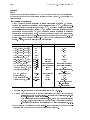
Modications of the system denitions
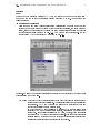
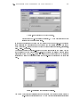
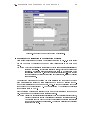
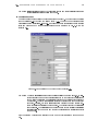
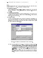
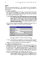
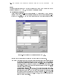
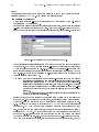
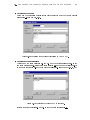
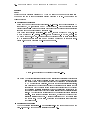
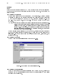
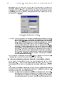
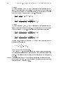
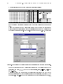
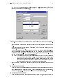
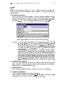
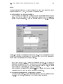
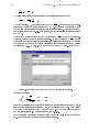
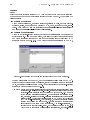
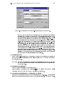
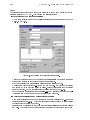
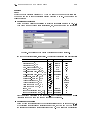
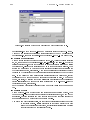
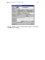
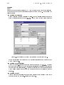
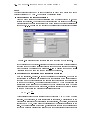
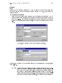
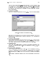
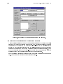
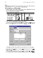
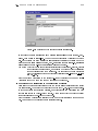
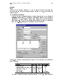
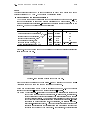
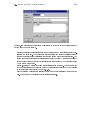
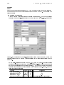
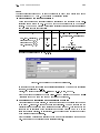
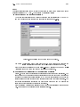
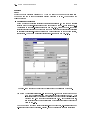
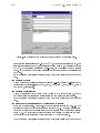
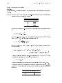
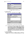
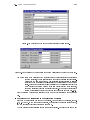
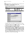
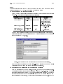
Dene a constant variable Cini with a value of 12 mg/l, a standard deviation of
1:2 mg/l, a minimum of 0 mg/l and a maximum of 100 mg/l. Activate the check boxes
active for sensitivity analysis and active for parameter estimation. Change
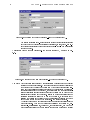
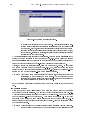
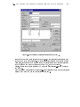
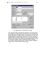
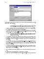
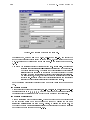
the initial condition for variable C in the compartment Reactor from Cmeas to Cini and
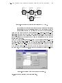
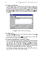
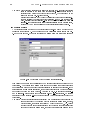
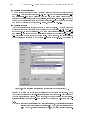
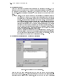
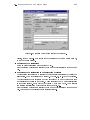
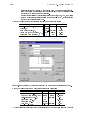
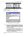
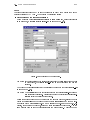
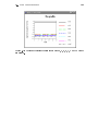
extend the plot denition Sens to contain a curve for the sensitivity of C with respect
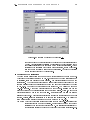
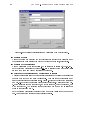
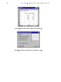
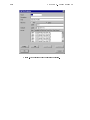
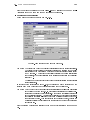
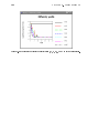
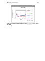
to Cini. Finally, duplicate the plot denition Sens, change the name to Err, for all
curves change the curve type from Sensitivity Function to Error Contribution,
and adapt the plot title and the ordinate label.
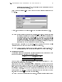
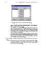
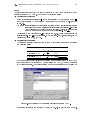
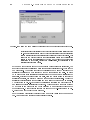
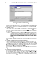
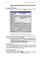
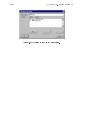
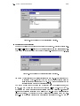
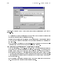
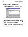
Save your system denitions to the le parest b.aqu by clicking the command File!Save As from the main menu bar and specifying the le name.
Execution of parameter estimation and sensitivity analysis
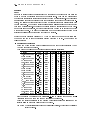
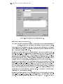
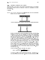
Redo the parameter estimation and the sensitivity analysis. The nal value of 2 is now
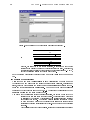
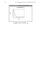
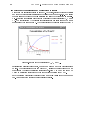
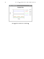
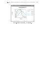
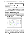
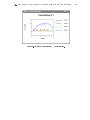
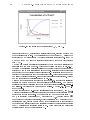
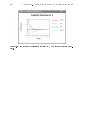
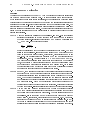
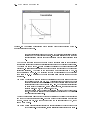
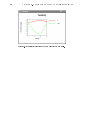
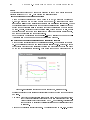
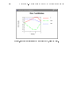
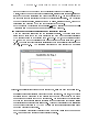
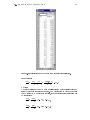
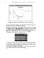
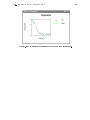
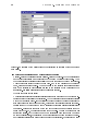
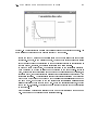
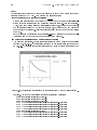
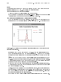
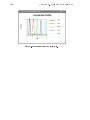
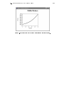
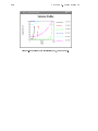
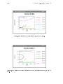
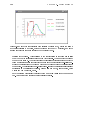
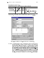
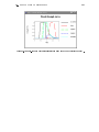
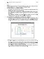
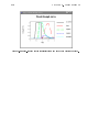
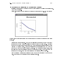
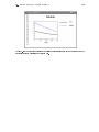
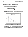
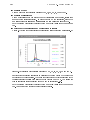
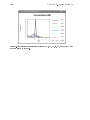
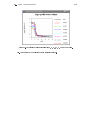
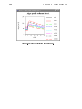
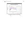
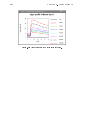
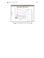
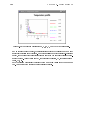
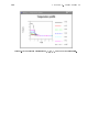
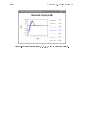
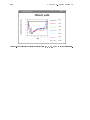
12.1, the correlation between K and rmax decreased slightly to 0.95. Figure 3.19 shows
the dierent behaviour of the sensitivity function of C with respect to Cini compared
to the two other sensitivity functions. This means that the new parameter Cini is
Figure 3.19: Sensitivity functions of C with respect to K, rmax and Cini.
identiable although there exists an identiability problem between the parameters K
and rmax.
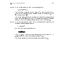
Comment: Note that the parameter estimation done in part B is much better than that of
part A because it considers the inaccuracy of the rst measurement at time zero.
Although usually only the parameters K and rmax are of interest, their estimates
can be improved by including the initial condition as an additional parameter to
be estimated.
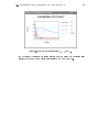
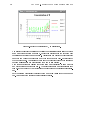
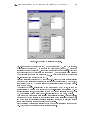
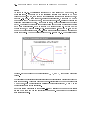
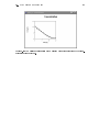
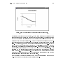
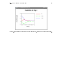
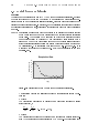
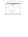
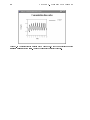
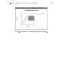
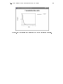
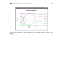
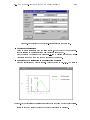
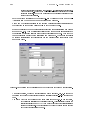
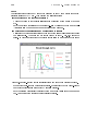
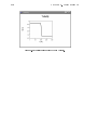
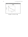
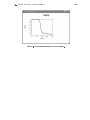
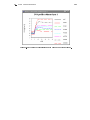
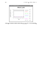
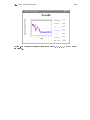
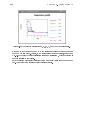
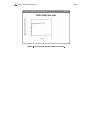
Plot now the calculated values (plot Conc). The result is shown in Fig. 3.20. Because