1
3D Multimedia Lab for Exploring Physics
Mechanics
Users Guide
DesignSoft
2007
I
Newton v3.0
Table of Contents
Part I Introduction
2
Part II Installation
4
1 Installation procedure
................................................................................................................................... 4
2 Uninstalling NEWTON
................................................................................................................................... 7
3 Network Installation
................................................................................................................................... 7
4 Copy Protection
................................................................................................................................... 8
10
Part III Overview
1 Screen layout
................................................................................................................................... 10
2 Running demonstrations
................................................................................................................................... 12
14
Part IV Getting started with examples
1 Demonstrating
...................................................................................................................................
free fall and making diagrams
14
2 Force and velocities
................................................................................................................................... 20
3 Fix Joint
................................................................................................................................... 24
4 Experiments...................................................................................................................................
with spring
25
5 Movement along
...................................................................................................................................
a straight line
27
6 Circular motion
................................................................................................................................... 28
7 Motion on spherical
...................................................................................................................................
surface
29
8 Incline
................................................................................................................................... 30
9 Planetary motion
................................................................................................................................... 31
10 Problems
................................................................................................................................... 32
37
Part V Usage of Newton in detail
1 Objects : Newton's
...................................................................................................................................
virtual building blocks
37
Simple bodies..........................................................................................................................................................
Dynamic Object
..........................................................................................................................................................
Constant .........................................................................................................................................................
force
Torque .........................................................................................................................................................
Fixjoint .........................................................................................................................................................
Spring .........................................................................................................................................................
Balljoint .........................................................................................................................................................
Hinge
.........................................................................................................................................................
Slider
.........................................................................................................................................................
Extra objects ..........................................................................................................................................................
Cannon .........................................................................................................................................................
Incline .........................................................................................................................................................
Matchbox.........................................................................................................................................................
Stand
.........................................................................................................................................................
38
39
40
41
42
42
43
44
45
45
45
46
46
46
© 2007 DesignSoft
Contents
II
Celestial body
.........................................................................................................................................................
(Cel. body)
Environment ..........................................................................................................................................................
objects
Background
.........................................................................................................................................................
Table
.........................................................................................................................................................
Camera .........................................................................................................................................................
Supplementary
..........................................................................................................................................................
element
Point
.........................................................................................................................................................
Velocity vectors
.........................................................................................................................................................
Acceleration
.........................................................................................................................................................
vectors
Track - the
.........................................................................................................................................................
path of movement
46
47
47
47
47
47
47
48
48
48
2 Editing in the...................................................................................................................................
3D window
49
Changing the..........................................................................................................................................................
point of view
Object manipulation
..........................................................................................................................................................
Adding, selecting
.........................................................................................................................................................
and deleting objects
Editing modes
.........................................................................................................................................................
Positioning,
.........................................................................................................................................................
rotating and scaling
Linking, anchoring
.........................................................................................................................................................
and fixing
Vector and
.........................................................................................................................................................
point editing
Cut, copy,.........................................................................................................................................................
insert, undo functions
3D Window settings
..........................................................................................................................................................
dialog
Units dialog ..........................................................................................................................................................
49
51
51
52
52
53
54
55
56
57
3 Properties window
................................................................................................................................... 58
Location
..........................................................................................................................................................
Velocity
..........................................................................................................................................................
Size
..........................................................................................................................................................
Inertia
..........................................................................................................................................................
Appearance ..........................................................................................................................................................
Material
..........................................................................................................................................................
Background ..........................................................................................................................................................
Table
..........................................................................................................................................................
Camera
..........................................................................................................................................................
Spring
..........................................................................................................................................................
Balljoint
..........................................................................................................................................................
HingeJoint ..........................................................................................................................................................
Slider
..........................................................................................................................................................
Fixjoint
..........................................................................................................................................................
Constant force,
..........................................................................................................................................................
Torque
Point
..........................................................................................................................................................
Cannon
..........................................................................................................................................................
Incline
..........................................................................................................................................................
Celestial object
..........................................................................................................................................................
60
62
63
64
65
66
67
68
69
70
71
72
73
74
75
76
77
78
79
4 Understanding
...................................................................................................................................
the simulation environment - running simulations
80
Force Field ..........................................................................................................................................................
Setting Simulation
..........................................................................................................................................................
Parameters
80
81
5 Description Window
................................................................................................................................... 83
General Usage
..........................................................................................................................................................
Insert line, ellipses,
..........................................................................................................................................................
pictures
Edit Text and ..........................................................................................................................................................
Equations
Icons of Text
.........................................................................................................................................................
dialog box
Text dialog
.........................................................................................................................................................
box | Speed menu
Sizes dialog
.........................................................................................................................................................
box
Creating Diagrams
..........................................................................................................................................................
Diagram properties
.........................................................................................................................................................
window
84
85
86
86
87
87
88
88
© 2007 DesignSoft
II
III
Newton v3.0
Interactive controls
..........................................................................................................................................................
Editfield .........................................................................................................................................................
Checkbox.........................................................................................................................................................
Radiobutton
.........................................................................................................................................................
Trackbar .........................................................................................................................................................
Button .........................................................................................................................................................
92
93
94
95
95
96
6 Creating Problems
...................................................................................................................................
and Problem Sets
97
Creating a problem
..........................................................................................................................................................
Creating a Problem
..........................................................................................................................................................
Set
Solving a Problem
..........................................................................................................................................................
Set
97
98
99
7 Printing and...................................................................................................................................
Exporting
100
Printing
Exporting
..........................................................................................................................................................
..........................................................................................................................................................
101
101
8 Newton Interpreter
................................................................................................................................... 102
Simple Mathematical
..........................................................................................................................................................
Expressions
Constants
.........................................................................................................................................................
and Variables
Mathematical
.........................................................................................................................................................
operation
Boolean.........................................................................................................................................................
operation
Mathematical
.........................................................................................................................................................
Function
Miscellaneous
.........................................................................................................................................................
Function
Browse Interpreter's
.........................................................................................................................................................
Symbol...
New Symbol
.........................................................................................................................................................
Multi-lined Expressions
..........................................................................................................................................................
Global Structure
.........................................................................................................................................................
Variables
.........................................................................................................................................................
Declaration and Assignments
Conditional
.........................................................................................................................................................
Statement
Loops .........................................................................................................................................................
Part VI Glossary
103
103
104
105
105
106
106
108
109
109
110
111
112
115
1 Command in
...................................................................................................................................
Menus
115
File
..........................................................................................................................................................
Edit (3D Window)
..........................................................................................................................................................
Edit (Description
..........................................................................................................................................................
Window)
View
..........................................................................................................................................................
Simulation ..........................................................................................................................................................
Problem
..........................................................................................................................................................
Windows ..........................................................................................................................................................
Help
..........................................................................................................................................................
115
116
116
117
117
118
118
118
2 Commands...................................................................................................................................
in Context Menu
118
3 Icons
Index
................................................................................................................................... 121
0
© 2007 DesignSoft
Part
I
2
1
Newton v3.0
Introduction
The virtual world of Newton v3.0 provides a completely new way of learning physics–the
exploration of kinematics and dynamics on a computer in 3D. The virtual world of Newton is
ruled by the simulated laws of physics, allowing you to build, manipulate and analyze your
experiments freely and interactively.
When creating an experiment in Newton, you can select from a wide range of real world or
abstract objects, from the simplest geometrical bodies (brick, sphere, etc.), complex
instruments (stands, slope, car, etc.), and constraints (many types of joints and springs). You
can adjust their physical parameters (mass, elasticity, friction, etc.); assign to them forces,
torques or velocity; and make relationships subject to constraints. You can add virtually any
object to Newton using a VRML editor; you may also export your experiments in VRML
format.
With the example files included, it's easy to get started. You can alter them and simulate
again, and you will see that it's quite simple to create amazing demonstrations.
When running a simulation, the bodies start moving, guided by the acting constraints; are
rotated by torques; and collide with each other as in a movie. Actually, you can set up one or
more “cameras” and capture their views of the experiment, storing them in an AVI file.
You can also add descriptions to your examples, with explanatory texts, images, and
formulas. Using diagrams, it’s easy to measure and evaluate the results of your experiments.
Several user-defined curves can be displayed on the same diagram, so it's easy to compare the
measured data with the results derived from theoretical calculations. You may also change the
units of the physical quantities.
© 2007 DesignSoft
Part
II
4
Newton v3.0
2
Installation
2.1
Installation procedure
Minimum hardware and software requirements
•
•
IBM PC Pentium or better
128 MB of RAM
•
A hard disk drive with at least 100 MB free space
•
CD-ROM
•
Mouse
•
24 bit true color, fast VGA graphics card with OpenGL Support
•
Microsoft Windows 98 / ME / NT / 2000/ XP
•
Novell Netware version 3.12 or later or MS Windows NT/ 2000/ XP Server or later
for the Network versions
If the program is copy protected by a hardware key, the minimum hardware configuration
includes also a parallel printer or USB port.
Installation from CD-ROM
To begin the installation, simply insert the CD into your CD-ROM drive. The Setup Program
will start automatically if the Auto-Run function of your CD-ROM has been enabled
(Windows-Default). If not, Select Start/Run and type:
D:SETUP (Enter) (where D represents your CD-ROM drive).
The setup program will start.
Note: This software may come with copy protection. For further details see the
Copy Protection and the Network Installation sections.
© 2007 DesignSoft
Installation
5
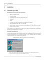
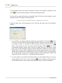
Following the Installation Steps
NEWTON’s Setup Procedure follows the steps standard with most Windows Programs. There
are several screen pages where you can enter or change important installation choices, such as
Type of Installation, Destination Directory, etc. To continue installation, click on the Next
button. You can always step back, using the Back button. If you do not want to continue
installation for any reason, click on the Cancel button. If you elect to cancel installation, the
program will ask you if you really want to exit. At this point you can either resume or exit
Setup.
Welcome and Software License Agreement
To begin the Procedure, click on the Next button on the Welcome Page. The first step is the
Software License Agreement.
Note: By clicking on “Yes” you are agreeing fully with DesignSoft’s Terms and Conditions
for using this software.
Entering User Information
This data is used to personalize your copy of the software. By default, the installation program
picks up the data entered when you set up Windows. You accept these names as defaults by
clicking on Next or you can change them.
Depending on your program version you might also need to enter a Serial Number located on
your CD-ROM package or on your Quick Start Manual.
Choose Destination Location
Here you can select an Installation Directory other than the one suggested as a default. The
default is the Windows Standard Directory for Programs. To change the directory, click on
Browse and select a different drive and/or directory from the Choose Folder Dialog.
© 2007 DesignSoft
6
Newton v3.0
Note: If you are installing NEWTON for Windows to a hard disk that already has
an earlier version of NEWTON, you must be sure to use a new directory name for
NEWTON for Windows, such as the suggested directory, C:\Program
Files\DesignSoft\Newton, or the working files you have already created will be
overwritten and lost. If uncertain, exit setup, copy your NEWTON files safely to
another hard disk directory or to floppy disks, then resume setup.
Completing the Setup
After all the selected files have been copied and the Start Menu entries created, you are asked
if you want to place a Shortcut to the NEWTON program file on your Desktop. The last page
indicates a successful installation and invites you to open and read a file with the latest
information about NEWTON. We urge you to take a moment and review that file. Click on
finish when you’re ready.
Note: You can read the latest information in the file again at any time by
selecting Read Me from the Newton Start Menu Entries. You can also get the
latest information about changes or new features by visiting our Web Site,
© 2007 DesignSoft
Installation
7
www.designsoftware.com.
2.2
Uninstalling NEWTON
You can uninstall NEWTON for Windows at any time. Note that this will not delete files you
have created.
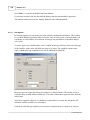
1.
To begin Uninstallation, choose Newton for Windows from the Newton Start-Menu
Entries.
2.
In the Window that appears, double-click on Uninstall Newton.
3.
Click on Yes if you are positive you want to uninstall Newton.
After all the files have been removed successfully, an OK Button appears. Click on it and
uninstallation is complete.
2.3
Network Installation
To install the Network version of NEWTON, you must log on to your server machine as a user
with administrative privileges (Novell 3.x: supervisor, Novell 4.x: admin, Windows NT:
Administrator). Then execute the procedure for the Hard Disk Installation on a disk volume
that is accessible from the network. Now carry out the following additional steps:
Make all files in the program and user directories sharable:
Novell 3.x:
FLAG *.* S SUB
Novell 4.x:
FLAG *.* +SH /S
Windows NT/2000/XP:
Depending on the setup of your system, you can give the rights to a group (<groupname>)
whose members will then have the appropriate rights automatically.
Next make sure that the clients have a mapped drive set to the network drive containing the
NEWTON program folder.
To assign (map) a drive letter to a network computer or folder do the following:
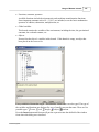
1. Open Windows Explorer
2. On the Tools menu, click Map Network Drive.
3. In Drive, select a drive letter e.g. G:
4. In Path (Win9x/Me/ or Folder (NT/2000/XP), select from the drop-down list or type
in the network drive (server and share name) or folder name to which you want to
assign (map) a Drive letter. Note, that share name refers to a shared folder on the
© 2007 DesignSoft
8
Newton v3.0
server. On Windows NT/2000/XP you can use Browse to find the network computer,
drive and folder.
5. Set the Reconnect at Logon checkbox.
6. Press OK
7. Examples:
Drive: G:
Folder: \\servername\sharename
or
\\MyServer\Volume1
\\MyServer\Volume1\Public
After you have set everything up on the Network disk according to the instructions above, you
must run the setup program on each Novell workstation where you want to run NEWTON.
Using the Run command, start NSETUP from the Newton\NWSETUP directory. Note, do
not double click on the NSETUP icon, but use the Run command instead to start the program.
When you run NSETUP, you must specify the working directory (which should be located on
a local drive of the workstation). The working directory can be on the network; however
in this case the path of this directory must be different on every workstation. After
running NSETUP, you will be able to run NEWTON simultaneously on any number of
workstations, just as though each workstation had a single user version.
2.4
Copy Protection
Software Protection
If your version of NEWTON is copy-protected by software, select Authorize from the Help
menu. For more information, choose Help from the Authorization dialog or open the file
'DSPNewton.hlp'.
Hardware protection
If you have a hardware-protected version, plug the dongle (hardware protection key ) into the
parallel (printer) or USB port connector. If you have a printer, connect it through this key.
Should you forget to connect the dongle, an error message will come up on the screen:
Hardware protection key is not present
Note: If you have a dongle-protected version under NT/2000/XP you should
install Newton in Administrator mode and restart the computer after installation.
© 2007 DesignSoft
Part
III
10
3
Newton v3.0
Overview
In this chapter we present NEWTON’s screen format, controls and menu structure.
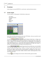
3.1
Screen layout
The user interface of the program is divided into six main parts:
3D Window
Description Window
Toolbars
Menus
Status field
Dialogs
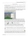
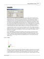
On the left side of the initial screen you can see the 3D Window, where you can edit or track
the ongoing experiments in a 3D perspective view.
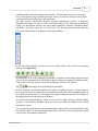
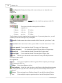
Use the
control buttons (Camera bar), to change your
point of view. Rotate the scene, zoom-in or zoom-out, and select special top or side views.
Even if a portion of the experiment is obscured from one vantage point, you can adjust the
camera and bring it into view. You can also rotate the scene by holding down the left mouse
button and moving the mouse, zoom in and out by holding down the right mouse button, or
shift the scene by holding down both buttons and moving the mouse.
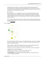
Using the
control buttons (Scene bar) and the mouse, you can modify
objects and their positions in the 3D window. The first two icons choose between the
geometric and physical editing modes. Using the geometric editing mode, objects can be
moved freely without regard for their logical and dynamic relationship to the other objects.
The Bodies can slide into each other without collision, and the constraint parameters can be
altered using the mouse.
Using the
physical editing mode, the bodies collide and slide against each other,
© 2007 DesignSoft
Overview
11
remaining on their track according to the constraints. The next three icons give you control
over vertical position, object rotation, and zoom setting. The last two icons are used to build
various relations among the object, link and anchor.
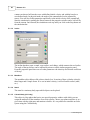
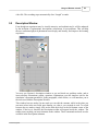
The right window (Description Window) presents explanations, pictures, or diagrams.
Diagrams can display the curves of the experiment based on the simulated or theoretical
results. The Description Window may also contain interactive elements, including buttons,
edit fields, radio boxes, check boxes, or track bars. The Description Bar presents icons that
you can use when editing or creating the Description Window.
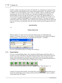
On the top of the application window you can see many toolbars. One of the most important
of them is the Object Bar.
It contains the icons of the commonly used bodies, constraints and auxiliary objects that you
can use in your demonstrations. The different types of objects are grouped on different tabs.
Click on an icon to pick up the selected object and place it into the 3D window.
The
toolbar helps you in performing file operations.
In some situations, pressing the right mouse button will bring on-screen a context menu to
give you quick access to commonly used commands related to the selected graphical object or
to the panel you clicked on. You can find these by right-clicking the objects in 3D Window or
the graphical objects of the Description Window.
One of the most important dialogs, which you can access by right-clicking or double-clicking
an object, is the Properties Window, where you can set or modify the attributes of the bodies
and dynamic objects.
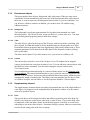
You can quickly toggle between open demonstrations using the tabs at the bottom-left corner
of the main window. In the bottom-right corner there is the Time field. It displays the elapsed
(virtual) time of the running simulation.
© 2007 DesignSoft
12
3.2
Newton v3.0
Running demonstrations
Newton comes with many prepared example demonstrations. Select the File/Open command
to load them.
When you load an example, the 3D and Description Windows will show the 3D experiment
and the explanations (if any) respectively.
You can rotate the point of view by clicking on a blank area of the 3D Window, holding down
the left mouse button, and moving the object to the desired position. If you click with the right
mouse button, you can step back and forward. You can slide up or down in the space by
moving the mouse and holding down both mouse buttons simultaneously.
Click on the
(Run) icon to start the simulation. The simulated laws of physics will guide
the bodies in their motion. To stop the simulation, click on the
(Stop) icon; it appears in
place of the Run button when an experiment is running. You can reset the scene by clicking
on the
icon.
The smoothness and speed of the motion depend on your computer speed and screen
resolution. If a simulation requires a lot of calculations, and your PC’s processor isn’t fast
enough, the simulation will not move smoothly and in realtime. In this case, use the
(Playback) function. It plays the last simulated demonstration smoothly and continuously
from the PC’s DRAM memory.
© 2007 DesignSoft
Part
IV
14
4
Newton v3.0
Getting started with examples
In this tutorial chapter, we will show you step-by-step how to use the program and how to
make convincing experiments and demonstrations. We recommend that you take the time to
walk through all the examples, not just read them.
The instructions for the first and second tutorials are detailed, while the later examples build
on the knowledge acquired from these and are not presented as thoroughly.
4.1
Demonstrating free fall and making diagrams
Our first example is very simple: you are to investigate the movement of a ball constrained by
the constant gravitational field of the earth. You will learn how to set the basic properties of
the bodies and how to depict their movement via diagrams. Later, the measured data will be
compared with the results derived from theoretical calculations. You can find this pre-built
example in the Freefall.ex example file.
Create a new experiment by clicking on the
(New) icon. This will call up empty 3D and
Description Windows and the screen shows only a tabletop.
Here’s how to modify the point of view in the 3D space: to rotate the vantage point, click and
hold the left mouse button on an empty area of the 3D Window and move the mouse in the
selected direction. To step forward and back (zoom-in and zoom-out), press and hold the
right mouse button. To slide in any direction, press and hold both mouse buttons. Note that
you can do the same but in larger steps using the
Perhaps you’d like a special top or side view of the scene – use the
to select another view, or the
toolbar controls.
toolbar buttons
button to revert to the general 3D view. Using the
control buttons (Scene bar) and the mouse, you can modify objects
and their positions in the 3D window. The first two icons choose between the geometric
and physical
editing modes. Using the geometric editing mode, objects can be moved
freely without regard for their logical and dynamic relationship to the other objects. The
Bodies can slide into each other without collision, and the constraint parameters can be
altered using the mouse.
Using the
physical editing mode, the bodies collide and slide against each other,
remaining on their track according to the constraints. For example, if a body is linked to a
hinge, it can move only on a circular track. Because more editing can be carried out in the
physical editing mode, it is the default. In the following instructions, you only have to switch
to the geometric mode if requested.
© 2007 DesignSoft
Getting started with examples
15
Let's start building our first simple experiment.
You can find the body named “ball”
on the Bodies page of the Objects toolbar. Click
on its icon and the body will immediately appear in the middle of the 3D area. To move the
ball to its initial position, use the mouse as follows. To change the location, press and hold the
left mouse button over the ball and move the mouse over the scene. This will move the body
in the xy plane and keep the z coordinate unchanged. To place the body properly in the z
direction, press down and hold the
icon and use the mouse.
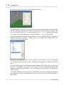
The properties of the ball can be set in the Object Properties dialog. This window will appear
if you double click on the ball.
The property window gives access to several pages of properties grouped according to
function. For example, on the Location page the position and rotation can be changed, while
on the Size page the size of the body can be reset. Each kind of object can have different
panels. Clicking on the body invokes the default page, showing the material properties group.
On the right side of the window there are icons which you can use to switch to another page
of properties.
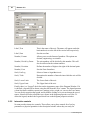
At the top of this window there is a combo box that contains a list of all the objects currently
present in the 3D scene. If you would like to alter its properties, select an object by name and
change the appropriate settings. In this list you will find, in addition to the object’s name, its
identity. All objects have a name and an identity, and they are not the same. The identity, as it
identifies the object, cannot be used with more than one object at the same time. It is a
combination of a short character string–generally an English word or abbreviation–and a
number. There are restrictions: special character cannot be used, for example +-*/[]() or
space. We will reserve these special characters for later use; for example, in defining curves
in diagrams.
The name of the object can be anything; it can contain more than one word; and the same
name can belong to more than one object.
You can easily change an object’s name or identity. Select the object and click on the
command 'Rename...' in the Edit menu. Alternatively, right-click anywhere in the properties
window and a context menu will appear with the command 'Rename'. Name the ball 'Rubber
Ball'.
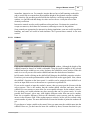
Click the
icon to bring up the Material panel. There is a combo box on this page with
commonly used materials. For material, select “Rubber” for now. There are other fields on
this page–density, friction, elasticity, etc.–but we will accept their default values now. Press
the Apply button to use these new settings.
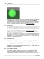
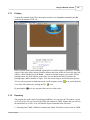
The color of the ball can be changed on the
below has been assigned a light blue color.
Appearance page. The ball in the picture
The dimensions of the body may be altered on the
(Size) page. Assign 10 centimeters to
the diameter (radius equals 0.05 meters) in the first field of the Size panel.
© 2007 DesignSoft
16
Newton v3.0
To assign a mass to the body, bring up the
Inertia panel.
Click on the
(Inertia) icon and set the value of Mass to 0.8 kg. Note that since an object’s
mass is directly proportional to the density, the density of the ball is changed as well.
Using the
(Location) panel, set the ball’s position to (x=0,y=0, z=2) or z=2m. Adjust the
scene by stepping back using the
icon until both the ball and the table can be seen.
Start the simulation. Click on the
(Run) button and watch the ball on the screen.
After falling briefly, the ball bounces off the table. Note that the simulation doesn't stop by
itself. To stop it, click on the
(Stop) button. Click on the
(Reset) icon to reset the
experiment environment to its pre-simulation state.
Making diagrams
Now let’s create diagrams to represent the motion of the ball.
In the middle of the table, a coordinate system indicates the origin of the 3D space. By
default, the positions versus time diagrams are made using this coordinate (reference) system.
The three gray axes that are drawn from the origin, perpendicular to each other, represent the
three (x, y, z) directions in the space. In this example, we will display the position of the ball
on the z axis as a function of time.
© 2007 DesignSoft
Getting started with examples
17
First, be sure that the Description window is in the Edit mode. This is the default for new
projects, but you can always switch to Edit mode using the Edit checkbox at the bottom left
corner of the Description window. When this window is in Edit mode, you should see the
vertical Description toolbar with icons to help you create the contents of the window.
Find the (Diagram) icon
and click on it to bring up the Diagram properties window. In
this context, you could create a curve and place it in a diagram in the description window. But
sometimes you want to just define an empty diagram to prepare for a curve that you will add
later. Let’s do that now.
Click the OK button. Place the diagram in the Description window as follows. After pressing
the OK button, a small coordinate system will appear on the canvas under the cursor. First,
move the mouse to the position where you want to place the top left corner of the diagram and
click there. After this the diagram size will change as you move the mouse. Moving the
mouse now will determine the bottom right corner of the diagram and if it is in its place, click
with the left mouse button again.
If you need to modify the size of the diagram, select the diagram by clicking anywhere within
its area, and move the graphic cursor above one of the little marking squares appearing in the
corners. Use the basic Windows mouse techniques to click and drag the marking squares to
their required places. Lastly, you can move the whole diagram by clicking within the diagram
area and dragging it with the mouse.
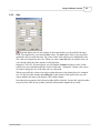
Now let’s add a curve to the diagram. Double click on the diagram area, and the Diagram
properties window will appear again. This is a two-page dialog. Clicking on the tabs at the top
you can change between the pages Curve and Appearance. On the Curve page you can
create, alter and delete curves, and on the Appearance page you can set the general appearance
of the diagram, such as the scaling of the axes, format of numbers, etc.
Select the Curves tab to activate its panel. There are two different ways to define a curve. We
will use the quicker and easier method, but its possibilities are limited.
Look for the tree view list in the upper part of the window. This presents the variable of the
scene object in a tree-structure. Clicking on the ball displays its physical variables, and
clicking on the position node expands the three components of the position vector. Select the
z component and click on the Add button below. This will tell the diagram tool to draw the
position z versus time. Click the OK button to apply this setting.
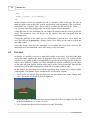
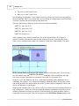
Starting the simulation again, we see Newton plot the vertical component of the ball’s
position versus time. The curve is a parabola, a parabola that corresponds to the motion of a
© 2007 DesignSoft
18
Newton v3.0
body accelerated by the gravitational field. Note that this curve was created with data obtained
using numerical methods.
Now let’s add the same curve, only created by theoretical methods. This will let us compare
the two methods. First, however, to make the theoretical curve, we have to use another
method.
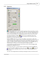
Bring up the Diagram Properties window again by double-clicking on the diagram. On the
Curves page click the Advanced button. This removes the object tree view from the screen.
Two text fields and some new buttons appear. These two text fields show the variables
assigned to the axes.
Select the previously created curve (“Position z”) and note the simple expressions in its edit
fields. In the previous step, where we selected the z-position of the ball, we have generated
the curve by actually filling in these expressions. Before creating more curves let’s study the
properties of this existing curve.
The Edit fields of this dialog are called Horizontal axis and Vertical axis. In each field there is
an expression already; „time” in the Horizontal axis and Ball.p[3] in the Vertical axis field.
When the simulation is running, these two expressions are evaluated at every time step, and
the two values together provide the point of the curve.
The ‘time’ expression is a global variable of the simulation; it defines the elapsed time from
starting. The ball.p[3] expression is a reference to the z component of the ball’s position. Here
the ‘ball’ is the identity of the scene object we are examining, ‘p’ means the position of the
ball and ‘[3]’ means the 3rd (z) component of the position vector.
All the other variables of the bodies and other objects can be used; moreover, you can use
mathematical functions.
You don’t have to remember all the available expressions and variables of your experiment. If
you click on the
icon, a dialog listing all the available and appropriate variables and
functions will appear. You can browse and insert them into the edit field by pressing the Insert
button.
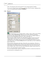
Now we are finally ready to make a new curve. Click on the Add button and write into the
© 2007 DesignSoft
Getting started with examples
19
fields the expressions shown in the figure below.
The word ‘time’ defines the horizontal axis variable to be the simulation time. The vertical
axis is assigned the expression
2-(9.81/2)*time^2, written as the equation z = z0 - 1/2gt2 in Newton. The term z0 = 2 is the
initial position of the ball.
You can write the expression in more than one row if this is more comfortable, but in this
case you have to use another form. Let's rewrite the example using this form.
var
z0 :real;
a :real;
begin
z0 := 2;
a := -9.81;
result := z0+1/2*a*time^2;
end.
This is a short piece of code in a Pascal-like language where between the begin...end rows you
can list your commands, such as 'z0 := 2;'. You must always include the line 'result :=... '; the
value of this expression will be plotted as the given axis point. Any variables you use must be
declared between the var...begin rows. Be careful that every command line is terminated with
a semicolon, and that a period follows the last 'end.' To learn more about writing simple or
multi-line expressions, see the chapter 'Newton Interpreter.'
Now we’ll change the color of the first curve we created. Select this in the Curve list and click
on the Properties button, which can be found in the right bottom part of the window. Set the
color to Red and the width to 3.
Close the windows and run the simulation again.
© 2007 DesignSoft
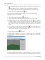
20
Newton v3.0
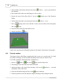
While the ball free falls to the table, the two curves overlap, as you can see in the picture.
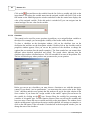
To set the axis properties, double-click an axis and work in the axis properties dialog that
pops up. For example, adjust the upper limit of the time axis to 1.6, and then close it using the
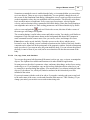
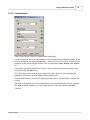
OK button.
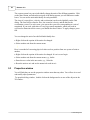
You can prevent the simulation from running continuously. In the Simulation menu, locate
the Time settings… command and click on it. In the window that opens, you will see the
Period panel. Set the “final time” checkbox on and set the time to 1.5s.
4.2
Force and velocities
In this chapter you can learn how to add constant forces to a body, how to adjust them using
the mouse in the 3D window, and how to assign an initial velocity to the body. This
experiment can be found in the file named ‘Const_Force.ex’.
Create a new example and place a ball
on the scene by clicking its icon on the Object
Toolbar. Move the ball to one of the table’s corners by double-clicking on the ball and setting
its position value on Location page of the Properties window. Type these values into the
position fields:
© 2007 DesignSoft
Getting started with examples
21
x=1m, y=1m, z=0.5m
Set the ball’s color to blue on the Appearance page. Set the z component of the velocity on
the Velocity page to 2m/s.
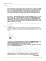
To verify the entries, click the check button under the edit fields to show the velocity arrow in
the 3D Window. You can immediately see in the 3D window that the ball now has a red
arrow emanating from the body’s center of mass.
There’s a more intuitive way to adjust the initial velocity. Using the mouse, select the vector
then click on the vector’s head by pushing the left mouse button. This will let you set the
vector’s direction. If you click on the vector’s shaft, you can change its magnitude.
When you need to set a property to an
exact value, use the Properties Dialog. Now let’s set the velocity to x=-1.5, y=0, z=1.7 m/s.
Next, we will add calibration ticks to the curve of the ball’s motion. Right click on the ball
and in the context menu choose the Show/ Track / Points command. Now the body will leave
markers along its path so we can examine the trajectory. Start the simulation. The ball falls to
the table in a parabolic arc, bounces up, and after a few more bounces falls off the table. Stop
the simulation
and press reset
to get back to the initial state.
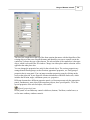
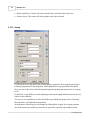
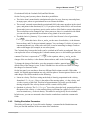
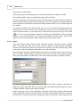
Clicking the
(Force fields) icon brings up the Force Fields window. Here you can set all
the external forces acting on the body: gravitational force, Coulomb force, and fluid
resistance. It can be seen that gravity is set to constant acceleration and its value is g =
9.81m/s2 as on the surface of the Earth. These are default settings in all new experiments.
Try the experiment with gravitation set to “none”. Click on the OK button and see what
happens. The ball will move along a constant line with constant speed, and won’t fall to the
table.
Stop the simulation and return to the original state by clicking on the reset button. Now we
will add a constant force acting on the ball. Select the body and click on the force icon
on the dynamics tab of the Object toolbars. In the 3D window you can see the blue force
vector originating from the body’s center of mass. You can alter the force vector in the same
fashion as seen earlier with the velocity vector. Click on the tip of the vector to set its
© 2007 DesignSoft
22
Newton v3.0
direction, and click on the shaft to set the strength of the force.
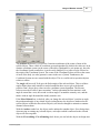
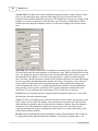
Add one more force to the body
Double-clicking on the Force’s blue arrow brings up the Properties dialog. From this dialog,
you can set the force’s parameters. Set the two constant forces with the help of this panel. The
first vector should be a force of 1N, and its direction x = 0, y = 0, z = -1, pointing downwards.
The second vector’s force should be 2N, and its direction x=1, y=0, z=0, (horizontal).
Start the simulation and observe that the body’s velocity is changing linearly, indicating a
constant acceleration. The body’s motion will stay in a planar zone, because there is no
velocity or force in the y direction.
Let’s make some diagrams of the vertical component of the motion. Click on the Diagram
icon on the Description window toolbar. The diagram dialog appears so that you can define
curves.
Choose the Ball/Position /z node and click the New button. This defines a new curve that will
draw the z component of the position versus time. Click on the OK button and place the
diagram on the Description Window. You can change the axis settings of the diagram by
double-clicking.
To compare a theoretical curve to the curve calculated by Newton, you can draw the analytical
and the numerical results on a single diagram. First, we’ll solve for the analytical solution of
this problem.
© 2007 DesignSoft
Getting started with examples
23
There is no gravitational force, so only the two constant forces accelerate the body. Since the
bigger force doesn’t contain a component in the vertical (z) direction, we need only take into
consideration the smaller force. Restating the problem, the Fz = 1.7 (N) force component acts
on the body and accelerates it in the z direction. The object has vz = 1(m/s) initial velocity
and z = 0.5 (m) initial position (we set these parameters earlier).
According to Newton’s second law ( F = m a ), the acceleration is:
a = F / m = -1 (N) / 0.1 (kg) = 10 (m/s2)
Next, we need the expression that describes the position versus time function of an object
with constant acceleration. This is the function:
s = 1/2 a t2 + v0 t+s0 ,
Substituting the values:
s = -5 t2 + 1.7 t+0.5 ,
Put a curve for this equation on the diagram. Click twice on the diagram area (not on an axis
or curve, because then the axis or the curve dialogs will appear). In the diagram properties
window click on the Edit button. The upper part of the window will change, the object tree
view disappears, and the two edit fields appear for directly defining the expression to the
diagram.
If you click on the curve created earlier you will see the two expressions of that curve. You
need to place the new expressions. Click on the new curve, and write in the horizontal axis
edit field:
time
And in the vertical axis edit field:
-5*time^2+1.7*time+0.5,
This format is required for Newton. The format below is perhaps more familiar, but they both
define the same equation, -5 t2 + 1.7 t+0.5 equation.
An alternative and more elegant way of defining this curve for the diagram is to store the
initial value of the ball's position and velocity instead of writing the numerical (1.7 and 0.5)
values directly into the expressions. For this we have to use multi-line form:
var
p0,v0 :vector;
begin
ifStartTime = Time then
begin
p0 := ball.p;
v0 := ball.v;
© 2007 DesignSoft
24
Newton v3.0
end;
result := -5*time^2 + v0[3]*time+p0[3];
end.
In this example we have two variables, p0 and v0, which are of the vector type. We store in
them the initial value of the ball's velocity and position at the beginning of the experiment,
when StartTime is equal to Time. The p0 and v0 variables are then used in the 'result := ...'
row. To learn more about writing code, consult the chapter 'Newton Interpreter.'
Using this form of curve definition you can change the position and the velocity of the ball
freely. The theoretical curve will always use the altered values and correspond with the
simulation curve.
Change the attributes of the earlier curve to differentiate it from the new curve. Select the
curve and click on the properties… button. On the Curve dialog set the color to yellow and
the width to three.
Close the dialogs and start the simulation. If everything has been done correctly, the
theoretical curve and simulation curves will exactly overlay each other.
4.3
Fix Joint
In Newton, it is possible to fix two or more bodies rigidly to each other. Now the bodies must
move and rotate together and share an aggregate mass and inertia. The motion of this
assembly is very similar to that of a simple body except that the material properties of the two
bodies can be different. Consider two cubes with different friction coefficients. Put the cubes
on the table and push, Repeat with the other cube’s surface facing downward. Note that the
friction force will be different depending which side is in contact with the table.
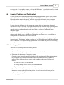
In this chapter you will learn how to build a gyroscope from a brick and a capsule rigidly
fixed together. The dynamic object you thus create will be called Fixjoint.
1. Get the brick and capsule from the Object bar and place them in the scene. Change their
color– the capsule to red and the brick to light blue.
2. Resize the bodies. The diameter of the capsule should be 0.03m, its length 0.3m. The side
of the brick should be x, y =0.4m, z=0.03m.
3. Get a FixJoint from the object bar and place it on the 3D window.
© 2007 DesignSoft
Getting started with examples
25
4. Select the three objects with the mouse and press down the
(Link to…) icon. This
causes the two bodies to be linked to the Fixjoint. The position of the FixJoint will be the
center of mass of the two bodies.
5. In Physical mode, dragging either of the two objects drags the other with it. The two bodies
’ relative position to each other can only be adjusted in geometric mode, so click on the
geometric
icon. Position the two objects according to the picture below.
6. Assign an initial velocity to the gyroscope. Since the bodies don’t have independent
velocity, only collective, their velocity cannot be altered individually on the Properties
window. The collective velocity can be changed on the FixJoint Properties window, at the
velocity page. Set to (-60,10, 750) -re. Their first two values mean a small change in the
exact rotation around the z-axis, which makes the motion of the gyroscope more
interesting.
7. Start the simulation.
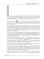
4.4
Experiments with spring
In this experiment, a force acts on a body via a (linked) spring. The force of the spring model
in Newton is composed of two parts; the first is a linear force in elongation that wants to
stretch the spring back to its unstrained length. In the second term the force overcomes
friction and is proportional to the velocity of the body. Expressed in an equation:
Here Dx is the difference of the actual length and the unstrained length, D is the stiffness, v is
the velocity, and b is the friction coefficient.
The behavior and use of the spring object will be explained in two examples. In the first, we
attach the spring to a stand and link it to a ball to examine harmonic oscillation.
1. Place a spring
object toolbar.
and a ball
on the scene clicking the appropriate icons of the
2. Select both the spring and the ball at the same time, and click on the
(Link to...) icon.
This links the spring to the ball. Note that you can select two objects at the same time by
selecting the first then clicking on the second while the CTRL button is pressed on the
keyboard.
3. To set the parameters of the spring, double-click on it and work within the Properties
Window that appears. Set the Stiffness of the force to 35N/m, and the unstrained length to
0.4 m.
4. Change the Location page of the properties window by clicking on the
icon. Adjust the z component of position of the spring to 0.8 m.
© 2007 DesignSoft
(Location)
26
Newton v3.0
5. Place the ball under the spring and lift the ball up. You can do this by pressing down the
(move up/down) icon. This constrains the ball movement to up and down only.
6. Go to the inertia page of the properties window and set the mass of the ball to 0.5kg.
7. Start the simulation by pressing down the
button.
Notice that the end of the spring that is not linked stays in rest during the simulation.
Let's include a stand in our experiment.
8. Place a stand from the Object toolbar
on the scene.
9. Drag the spring under the Stand and lift it up until it touches the bar of the stand.
10. Anchor the spring to the stand. Select the spring. Then click on the
icon and then on
the stand. Moving the stand now will drag the spring with it. To cancel the anchor, first
select the body, then press down the anchor icon, and click anywhere on the background
of the scene. You can also work with anchors from the Location page of the Properties
window.
11. You can change the width of the spring. Press down the
icon and move the cursor to
the spring. Adjust the spring width by moving the mouse up or down. Note that this
changes only the appearance, not the mechanical behavior.
12. Start the simulation with the
(Run) button.
The default setting of damping is zero–there is no damping. You can set the damping
coefficient from the spring page of the properties window by double clicking on the spring.
Try the value 0.1
The unstrained length of the spring can be set while viewing the 3D window. Lift the ball to
the desired unstrained position, click on the spring with the right mouse button, and select the
© 2007 DesignSoft
Getting started with examples
27
unstrained length command from the context menu. This results in the actual size of the
spring also being the unstrained size.
The following example is more complex, using three balls and three springs.
(Springs_with3ball.ex)
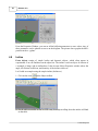
1. Create a new example and place three balls and three springs on the table.
2. Set the mass of all three balls to 0.1kg and the unstrained length of the springs to 0.6m
Link the balls to the spring as illustrated in the screen shot to the left.
3. Start the simulation.
In this example the ball-spring system is symmetric. You can adjust the unstrained lengths
and the masses to try variants of this example.
4.5
Movement along a straight line
Frequently we will want to examine problems where motion is confined to one dimension.
There is a constraint in Newton that reduces the six-degree of freedom case to only one. This
object is a constraint called Slider. It will force the object to stay on a straight line.
If we link two bodies using a Slider, they will move together except for the distance between
them, which can change freely. It is as though the bodies are skewered on a shaft and can only
slide along its axis.
This constraint is well suited to an examination of one-dimensional motion. In this example, a
ball and spring will permit us to examine the one dimensional harmonic oscillation.
Let’s get started making an example (1DSpring.ex).
1. Place a
ball and a
slider on the scene.
2. Select the ball and change its color to red on the
window.
© 2007 DesignSoft
(Appearance) page of the Properties
28
Newton v3.0
3. Select both the slider and the ball and click on the
the constraint.
(Link to…) icon, to put the ball on
4. Place another ball on the scene and change its color to yellow.
5. Increase the mass of the yellow ball to 2 kg on the
Dialog.
6. Link the ball to the slider; select both and click on the
7. Place a
and click
(Inertia) page of the Properties
(Link to…) icon.
(Spring) on the scene and link its ends to the two bodies (Select all together
icon).
8. Set the friction coefficient of the bodies to zero.
9. Start the simulation (
Run ).
Explore this experiment by stiffening the spring (see the chapter ‘Experiments with springs’).
4.6
Circular motion
The dynamic object called Hinge constrains the body to move in a circular track. If we link
two bodies to the hinge, we have modeled the linkage used for the rear wheels of cars.
Let’s build a pendulum utilizing the hinge. (Pendulum.ex).
1. Retrieve a
stand, a
ball, and a
hinge from the Objects bar.
2. Lift the hinge to the end of the stand’s horizontal shaft.
3. Anchor the hinge to the stand. Select the hinge, click on the
immediately click on the stand.
4. Select the ball and the hinge and click on the
(Anchor to…) icon and
icon to link them.
5. Switch to geometric mode and adjust the length of the hinge rod by lifting the objects.
© 2007 DesignSoft
Getting started with examples
29
6. Return to physical mode and set the initial angle of swing.
7. Start the simulation (
).
Go to the Properties window where the hinge’s parameters are set. You can draw any of these
parameters on a diagram, and they all can be reached from the Diagram dialog. In the diagram
window above we have presented a curve showing the angle of swing of the pendulum.
4.7
Motion on spherical surface
You can constrain a body to the surface of a sphere by linking the body to a balljoint. A
balljoint constrains the ball to remain at a constant distance from a point; however, the body
can rotate freely around the joint.
We can make another pendulum, this time using the balljoint (Pendulum_withballjoint.ex).
1. Place a
scene.
stand, a
ball and a
2. Select the balljoint, click on the
stand.
balljoint from the object toolbar onto the 3D
(Anchor to…) icon, and immediately click on the
3. Select the balljoint and the ball and click on the
to link them together.
4. Switch to geometric mode to adjust the position of the ball. Place it under the balljoint.
5. Switch back to physical mode and drag the ball to its initial position.
6. Set the initial velocity of the ball. If you don’t do this, the swinging ball moves in a plane.
Now we want the plane of the swinging ball to rotate. To achieve this, assign a velocity to
the ball perpendicular to this plane.
7. Start the simulation by clicking the
© 2007 DesignSoft
(Start) icon.
30
Newton v3.0
From the Properties Window, you can set all the balljoint parameters to exact values. Any of
these parameters can be plotted as curves on the diagram. The picture above graphs the ball’s
position in the x–y plane.
4.8
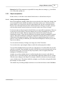
Incline
Extra objects consist of simple bodies and dynamic objects, which often appear in
experiments. You will find these on the object bar. The incline is such an object. It consists of
a rectangle, a hinge, and an incline-base. It has its own Object Properties window where the
angle, the friction coefficient, and elasticity of the incline can be set.
Let’s build an example using the simple incline (Incline.ex).
1. Click on the icon
in the Object toolbar.
2. Set the table next to the incline in such a way that objects rolling down the incline will land
on the table.
© 2007 DesignSoft
Getting started with examples
31
3. Set the angle of the incline by moving the flat of the incline.
4. Add a brick
to the experiment.
5. Change its color from the
(Appearance) panel.
6. Pull the brick up the incline until its bottom surface fits onto the surface of the incline
perfectly.
7. Set the friction coefficient. Click twice on the body, the incline and the Table, set the
values required on the Object Properties window.
8. Start the simulation by clicking on the
4.9
(Start) button.
Planetary motion
Up to now we have only made experiments in the gravitational force field of Earth. Using
Newton, it is possible to set the gravitational field so the bodies attract each other according to
Newton’s gravitational law,
. This will allow us to demonstrate planetary motion. In
this chapter we will show the detailed steps required to simulate our Solar system
(InnerPlanets.ex). This simulation is quite different from those seen up until now, because the
values of distance coordinates and time magnitudes are vastly larger. Try to imagine the huge
distances that separate the planets, and the time scales of their periods. The main task in
creating this experiment is to set the magnitudes of time and space parameters.
1. Create a new example and set the table visibility parameter to false.
2. Click twice the background of the 3D window, in an open area. The Properties window
appears–select the starry night sky.
12
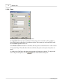
3. Set the Dimension value to 10 (type: 1e12) in the View menu 3D window settings
dialog. This setting affects mouse movements in the 3D window. Bigger values make the
same mouse movement cover far greater distances in the virtual space. You can travel
millions of virtual kilometers with a single mouse gesture.
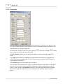
4. Set the gravitational force to planetary in the Simulation menu Force fields
dialog.
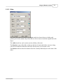
5. Change the unit system to astronomical by selecting it from the combo box in the
Simulation menu Units dialog.
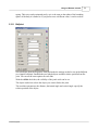
6. In the Simulation menu Setting… command invoke the Settings dialog, set the virtual time
to one day, and the time step to 0.01 day.
7. Click on the
(Planet) icon in the extra objects tab on the object bar.
8. Select the sphere object, and double click on it to bring up the Properties Window. Choose
one of the planets or the sun from the Object name combo box. Newton automatically sets
© 2007 DesignSoft
32
Newton v3.0
the astronomical body’s real properties.
9. Insert as many objects as you want (don’t forget the Sun), repeating the previous step.
10.The two trackbars on the Properties window are useful for scaling the size of the Sun and
the planets. Note that this scaling doesn’t alter the mass or the density parameters. It’s
meant only for improving the view of the solar system.
11.On the bottom of the panel you can set the Date, which will affect all of the object
positions.
12.Choose a good location in the universe where you can see all the objects, and run the
simulation.
Note: During editing in this experiment, it is possible to inadvertently get inside an
object while moving the camera, Of course we can’t find that object because from
the inside it is transparent. If this happens, use the camera positioning controls or
the camera properties window to get out of the object.
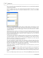
4.10
Problems
This chapter shows how to start with an existing example file and transform it into a new
problem file.
Just as with example files, problem files contain 3D window(s) in which the problem is
illustrated, and description windows. Problems can be presented using both types of windows.
You may also use the description window to present some hints or even a solution to help the
problem-solver.
We will now alter the free fall example into a problem. The task for the student will be to
answer a few questions. Follow the steps below:
1. Open the Freefall.ex file.
© 2007 DesignSoft
Getting started with examples
33
2. Delete all the text except the title.
3. Place this text below the title :
’A body is dropped from a height of 2 meters.’
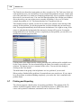
4. In the first question (problem a) the student has to choose the right value from the possible
answers. The text of the question is:
Findtheaccelerationofgravityontheearth!
We’ll use
(radio buttons) to make this a multiple-choice problem. You will find radio
buttons on the description toolbar. Place one on the description window and double click on
it. The radio button properties dialog appears with which all the settings can be adjusted.
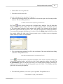
Enter three answers into the row list: 2, 9.81, 100. One of these has to be the right answer.
You must tell the program which answer is correct. Select the Right value field and write the
line number holding the right value. Newton permits you to calculate scores–an important
feature when you create a set of problems.
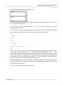
5. The second question (problem b) will be the calculation of the time the ball takes falling
to the floor. The problem text is:
Findthetimewhentheballreachesthefloor!
Use the
(editfield) element for this kind of problem. Click on the icon in the toolbar, put
it into the description window, and click twice on it. In the properties window, chose the Use
in questionnaire option to enter the right value (0.64 second in this problem), and assign a
tolerance of 0.03. (This means that the acceptable error is 0.03/0.64 = 5%). Finally, enter the
point value for scoring this problem.
6. The third task (problem c) is to solve a yes-no question. The problem text is:
Iftheanswerisright,checkthebox!
© 2007 DesignSoft
34
Newton v3.0
For this multiple choice test, the best descriptive element is the checkbox component. Click
on the
icon on the toolbar and place it onto the description window.
Let’s give this a caption that asserts a questionable truth. Click twice on the checkbox and its
properties window will appear. Enter the caption:
The acceleration of the ball doesn ’t depend upon its mass.
Check the right value of this statement to true, and enter the point value for scoring this
problem.
7. It is possible to give hints to help the student solve the problem. Click on the
(Create
new Page) icon at the bottom of the description window. Each time you click on this icon,
a new page is created. It is possible to delete the page currently on-screen with the
(
Delete Actual Page) icon. You can move among the pages with the
icon. To tell
Newton that the page contains a hint, you have to change the type of the newly created
page. Click on the description window with the right mouse button and in the context
menu choose Set page as/Hint command. Newton’s scoring system allows you to define a
penalty when a student needs a hint. His/her score will be reduced by a given percentage.
To set this number, click on the description window with the right mouse button, and
choose the Hint Score Reduction… command in the context menu.
8. It is also possible to provide the full solution. However, if the student looks at it, her score
on this problem is set to zero. Create a new page , write the solution, and right-click on
the description window. In the context menu choose Set page as/Solution command.
© 2007 DesignSoft
Getting started with examples
35
9. When you have completed the problem file, you can save it. In the Save dialog, change the
filter of the file type to ‘Newton problem file *.pb’.
When you next reload the file, Newton will determine automatically that it is a problem file
and switch to problem solving mode. All editing operation will be prohibited and in place of
the Object bar, Newton will present the Problem control. The student’s answer can be entered
for the interactive elements, and hints and solutions can be fetched using the two buttons of
the status bar of the description window. To test a value entered by the student, click on the
Submit button on the problem tool bar.
To switch back to editing mode, click on the Problem menu Edit command. Entry to the Edit
mode is password protected so that students will be prohibited from checking their answers or
otherwise manipulating the test. For all problems there is only one password. Its default value
is ‘Newton’, and, of course, you can change it. If you forget your password, reinstall Newton
(be careful not to overwrite your own experiment and problem files) to set the password again
to the default.
If you have a number of problem files covering the same material, you can bind them into a
set of problems. The resulting problem set can be used for student testing. You can do this
clicking on the File/Problem Set Manager… command, which will invoke a dialog where
you can set up the details for the problem set. The extension of a problem set file is ‘*.pbs’.
© 2007 DesignSoft
Part
V
Usage of Newton in detail
5
37
Usage of Newton in detail
In this chapter we will introduce and explain Newton’s tools and their use. We will guide you
through the objects that can be used to build your experiments and explain their functionality
and properties. We will show you how to easily and quickly use objects to create accurate,
stable and fast simulations.
You will also learn how to create powerful description windows using diagrams, explanatory
texts, and interactive elements. We will demonstrate making output files formatted as a vrml
model file or as an avi video file.
To create a new experiment click on the New
icon on the Standard toolbar or on the New
command in the File menu. You can save the current file with the Save
icon or the Save
command in the File menu.
5.1
Objects : Newton's virtual building blocks
We will typically use several elements to realize our experiments; these elements are called
Objects.
The Objects can be classified into the following groups:
· Simple body (e.g., ball, brick, octoeder)
· Dynamic objects (e.g., force, spring, joints)
· Extra objects (e.g., incline, seesaw, matchbox)
· Environmental objects (e.g., table, background, camera )
· Supplementary element (e.g., track, velocity vectors, points)
The first three groups can be found on the Objects toolbar. This bar has three pages, one for
each group. You can switch among them by clicking on the tabs. Click on an icon to add a
new object to the scene. Newton will place it temporarily in the middle of the window.
The supplementary elements cannot exist unless incorporated into one of the simple bodies or
extra objects. The track (which displays the trajectory of its body) is an example of this kind
of object. Its properties can be manipulated by the properties window or by the context menu
of its 'parental' objects.
The environmental objects generally play a passive role in the experiment. They make the
scene attractive and aid in editing operations. When you create an experiment from scratch,
Newton automatically provides these (environmental) objects.
All objects–except the supplementary ones–have their own identifier and name. Extra
objects may contain several simple bodies and dynamic objects, so each parts have its own
name and identifier. The identifier and the name are not the same! Each object has a unique
© 2007 DesignSoft
38
Newton v3.0
identifier, which is not used by the others. The identifier is a combination of a short character
string, (generally a short English word or abbreviation), and a number. The identifier is used
to define a curve for the diagrams, where we have to identify an object and their parameters
unambiguously. Because these identifiers are often placed in mathematical formulas, we
should confine ourselves to using only the letters [a..b] and [A..B] and the numbers [0..9].
The first character of the identifier cannot be a number. Object Identifiers in Newton are not
case sensitive–redball22 and RedBall22 are interpreted as the same. The name of an object,
on the other hand, can be anything. It may contain several words and more than one object can
have the same name. In the program, the name and the identifier generally appear beside each
other, as:
name[identifier]
e.g.
Billiard Ball [ball1]
When creating a new object, Newton will automatically assign it a default name and
identifier. If you move the mouse over the object, the default name and identifier will appear
in the status bar. To alter the strings, use the Edit menu/ Rename... command.
Now let's go through the objects according to their category.
5.1.1
Simple bodies
The most common building shapes can be found on the Bodies page of the Object Bar. In
Newton, we use the term body for any object that has material. This kind of object has mass,
density, and inertia properties; the bodies can collide and slide with each other; may have
charge; and are affected by gravitation. Simply put, these are the commonly known bodies of
our ordinary, real world. Newton offers the following basic shapes:
There are still more body models in Newton’s 'models' folder. These files have a '.o'
extension. To browse these models, click on the library icon
on the bodies page to
invoke the model dialogs. Select a body model and click the OK button to create an instance
of that model in the 3D window.
© 2007 DesignSoft
Usage of Newton in detail
39
If Newton doesn’t have the body shape model you need, you can use 3D modeling software
(available from other vendors) to create the model. The program you choose must be able to
export models to the prevalent standard, the so-called VRML 2.0 (Virtual Reality Modeling
Language 2.0).
Pay attention to these aspects of model creation:
The body should be a one piece, continuous, closed-surfaced shape. It doesn't matter that the
vrml file may contain several shape elements, but the elements together must comprise a
polygon with a one piece, continuous, closed-surfaced shape. In addition, the following
requirements must be respected:
·
The normal vectors of each polygon face must point outward.
·
There must not be any duplicate faces.
·
All face sides must connect to another face.
If these requirements aren’t met, the volume and mass calculations cannot be executed or will
be wrong. There is no way for a program to convert an unclosed surface to a continuous,
closed-surface body.
The imported body automatically gets default material properties, which can be changed
later.
In some simulations, bodies collide with each other, which in general requires a great deal of
processor resources and can significantly slow down the simulation. The special shapes–ball,
brick, cylinder, capsule, etc.– are computed differently, and their collision calculations
execute faster and with greater accuracy. Collisions involving the other bodies are calculated
on the basis of the location of the polygons, and the required calculation time is proportional
to the square of the number of faces. When using these bodies it’s best to reduce the number
of faces. Wherever possible, we can use passive elements in the simulation, which don't
collide. For passive bodies, reducing the number of faces is not so important because only 3D
drawing slows down, and drawing is generally so fast (aided by the PC’s graphics card), that
the slowdown isn’t noticeable.
5.1.2
Dynamic Object
In Newton the constraints and forces acting on a body can be defined by dynamic elements
placed in the 3D window and linked to the bodies. These objects, although appearing in the
3D window, don't have material properties and cannot collide with other bodies. Their shape
only illustrates their functionality and helps to understand the configuration of the experiment.
These dynamic objects can be used in our demonstrations:
· force, torque
· spring
· constraints: ball joint, hinge, slider
© 2007 DesignSoft
40
Newton v3.0
· fix joint
Every dynamic object must be attached to one or more bodies to have an effect. The constant
force or a torque can be assigned to only one body, whereas the springs and joints can control
the motion of two bodies simultaneously. These objects have two connectors, but they also
work with one connected body; in this case, the free connector will be fixed to its current
position. The fixjoint, which clamps bodies together, requires a minimum of two, and can
accommodate an unlimited number. The glued bodies will behave as one during the
simulation.
By default all of the dynamic connections are visible and appear in the 3D window. You will
notice “symbolic rods” between the centers of mass of the body and the dynamic object. It
must be emphasized that this is a virtual rod, so, for example, it has no mass property and is
unable to collide. The rod only shows the relation between the two objects to make the scene
more understandable. You can hide a symbolic rod by right clicking on it and unchecking the
visible command in the context menu.
In the next section, we will examine the functions of these elements and get a better feeling
for their use.
5.1.2.1
Constant force
According to Newton's second law, a constant force will accelerate a body. To create and
attach a new constant force, select the body and click on the force button on the object toolbar
(dynamic tab) . A blue vector, starting from the center of mass of the body, appears in the 3D
window.
You can alter its direction and magnitude using the mouse (see Vector editing chapter), or by
adjusting the related parameters on the properties window's force panel. To place this
property, click twice on the blue force vector in the 3D window.
You can assign more than one force vector to a body. The program computes the resulting net
force according to the parallelogram law.
By default, the point at which the force acts is the center of mass, but this isn't a requirement.
It can be attached to any point object (from the supplementary object group) that was
assigned previously to the body, and can be placed anywhere inside or outside of the body or
on its surface. To place the acting point of the force outside the center of mass, you should
first create and reposition a point object, then select it and click on the force object in the
object bar. Note that you can also change the position of the acting point on the force panel.
Using this method, Newton will automatically create the acting point and make it the
currently selected object. You can read more about point objects in the Supplementary
© 2007 DesignSoft
Usage of Newton in detail
41
objects chapter.
There is one vector visualization issue left to discuss. How big (or little) should the force
appear on the screen? This question arises because the size of the force is expressed in [N]
(using the SI system), while the representation of the force vector should have a length
measured in [m]. We need a rate number with which to multiply the size of the force to get
the length for screen presentation:. On screen, the force vector will be represented by a blue
arrow in the scene alongside the body upon which it bears. Multiplying all the vectors with
the same rate number makes sense, because the force vectors will maintain correct proportion
to each other, their size can be compared on the scene, and vector addition can easily be
visualized. But the rate number cannot be arbitrary: use too big a rate and the screen will be
overgrown by the vectors; or use too small a rate and the vectors will be hardly noticeable or
hidden by the bodies. You can change the rate number of forces and other kinds of vectors–as
long as the vector units are not length type. Velocity and acceleration, for example, can be
used with a rate number.
On the Unit dialog (Simulation/Unit command), besides setting the unit used in Newton
dialogs, you can set the rate number of three parameter fields related to the vectors: force,
velocity, acceleration. These incorporate the rate number, which can be altered here. If you
enter a value two times bigger into the force editfield, the force vectors on the scene will
double in size.
5.1.2.2
Torque
Torque is a force that acts upon the body and produces angular acceleration inversely related
to its inertia moment. Visually, the torque object is very similar to the force vector, except for
a rotation indicator around the head. The direction and the size of the torque vector can be
adjusted with the mouse or by the torque panel on the Properties window (double click on the
© 2007 DesignSoft
42
Newton v3.0
torque). The length of the torque vector in the scene is scaled by the rate number of the force
(see Unit dialog).
5.1.2.3
Fixjoint
The fixjoint joins two or more bodies together. After you attach two or more bodies to each
other, Newton inserts a fixjoint at the center of mass of the aggregated bodies. The bodies
connected by the Fixjoint move and rotate together as though they were a simple rigid body
with the total inertia. When you link two or more bodies, the resultant initial velocity and
angular velocity are automatically computed. If you want to adjust the velocity, you will have
to set the velocities of the Fixjoint. Newton makes the velocity properties of objects read only,
so you cannot give initial velocity or angular velocity to composite bodies. Of course, you can
modify the material properties of the individual components separately.
5.1.2.4
Spring
© 2007 DesignSoft
Usage of Newton in detail
43
The spring object acts upon one or two bodies with a force directly proportional to the
difference between its unstrained and current length. Both bodies can rotate freely because
they maintain their inherent degrees of freedom. The physical spring model contains a friction
component, which is proportional to the velocity.
where D is stiffness, is Dx elongation between the current and unstrained lengths, b is the
friction coefficient, and v is the difference of the velocity of the two bodies. The stiffness,
unstrained length, and friction parameters can be controlled on the spring panel. Setting the
friction coefficient to zero gives you an ideal spring , which can be used, in creating an ideal
harmonic oscillator.
You can link the spring not only at the center of mass, but to any other Point (supplementary
objects) assigned to the body. The spring acts upon the selected body through this acting point
(See the Point chapter).
5.1.2.5
Balljoint
If you attach a body to a point in space by a fixed length rod and let it rotate freely around the
point, you constrain the body to the surface of a sphere. The balljoint acting upon its linked
bodies realizes this constraint.
When two bodies are linked to the balljoint, both are able to rotate around the balljoint. In
addition, the three linked objects can translate and rotate together freely.
In addition to Cartesian coordinates, the position of a linked body can be given in spherical
coordinates relative to the joint location:
l distance : distance between a body and the joint (length of the rod)
Q vertical angle : angle between (0,0,1) and a rod to the body
d horizontal angle : if you project the rod into the xy plane, this is the angle between the
(1,0,0) axis and the projected rod
© 2007 DesignSoft
44
Newton v3.0
While a simulation is running, the length of the rod remains constant, but the two angles
change as the simulation progresses. These coordinates can be plotted on a diagram as
functions of time. You can alter these parameters numerically on the balljoint panel of the
properties window.
5.1.2.6
Hinge
If you link a body to a hinge, it can freely rotate around the axis of the hinge ( a ) at a constant
distance; namely, on a circle.
In the case of two linked bodies, the bodies can rotate around the hinge axis, and together the
three objects can move and rotate freely.
The position of a body, in addition to its usual Cartesian coordinates, can be described relative
to the hinge by three new coordinate values.
l distance: distance between the body and the hinge (length of the rod)
d angle : angle between the axis a and the rod
Q rotation: If you rotate the body around the a axis, you will find a location where the z
component of the body position is the biggest. This is the zero rotation point, and this rotation
parameter is measured from that point.
During simulation time, only the rotation will change–the distance and angle remain fixed.
However, these parameters can be plotted on diagrams and can be changed on the properties
panel of the hinge.
© 2007 DesignSoft
Usage of Newton in detail
5.1.2.7
45
Slider
A body has six degrees of freedom in 3D space; three belong to translation and three to
rotation. Sometimes, in the interest of simplicity, you may want to examine the movement in
only one dimension. Perhaps you’d even dispense with the three rotational degrees of freedom
in the interest of simplicity. The slider dynamic object will handle this requirement.
The slider keeps the linked bodies on a line ( a direction vector). The body can slide upward
or backward along the straight path, but it's unable to leave it.
If you attach two bodies to the object, they can also slide along the line freely, but the three
objects must stay together as they move and rotate.
The center of the slider object is always at the midpoint of the distance of the bodies ( a ). All
parameters ( a , l ) can be adjusted on the slider panel of the properties window.
5.1.3
Extra objects
Several special or frequently used objects can be found on the Extra object tab of the object
bar. Most of these objects were created using the dynamic objects and bodies. As they are
often used in demonstrations and make the development of demonstrations easier and faster,
we made them before we made the demonstrations. Some of these extra objects have unique
capabilities that can be controlled on their properties window (see Properties window chapter)
. Let's walk through these objects one at a time.
5.1.3.1
Cannon
You can easily demonstrate projectile motion with the cannon object. It has three parts: a
stand, a cannon barrel, and a hinge, which connects the stand and the cannon barrel. The
© 2007 DesignSoft
46
Newton v3.0
cannon can shoot a ball into the scene with defined initial velocity and with the barrel at a
user-defined angle. In physical mode, the angle of the cannon barrel can be adjusted by
mouse. You can also set this parameter numerically to the initial velocity of the cannon ball.
Start the simulation by pushing the Shoot! button on the properties window and a ball will fly
from the cannon. Once started, the simulation won't stop until you click on the Stop button on
the simulation bar.
5.1.3.2
Incline
The incline has three parts: a stand, a top surface, and a hinge, which connects the two bodies.
The angle of the top surface can be adjusted by mouse or on the incline properties panel.
From the properties panel there are two other parameters–the elasticity and friction coefficient
of the top.
5.1.3.3
Matchbox
The matchbox object behaves like a three-wheeled car. It consists of three cylinders (wheels),
three hinges and a simple frame. If we set its initial velocity, it will roll on the surface (table,
etc.).
5.1.3.4
Stand
The stand is a stationary body upon which objects can be placed.
5.1.3.5
Celestial body (Cel. body)
This object is a big sphere that has its own special properties window with which you can
assign the attributes of the members of our solar system. Choose your planet and place it at a
given time with the right mass and rotation velocities. It’s easy and fast to simulate our Solar
system using the Celestial body.
© 2007 DesignSoft
Usage of Newton in detail
5.1.4
47
Environment objects
This group includes three objects: background, table, and camera. When you open a new
experiment, Newton automatically places one each of the background, table, and camera on
the scene. A scene accepts only one background and one table, so you can’t add them. You
can, however, add more cameras; in addition, you can have more 3D windows using
additional cameras.
5.1.4.1
Background
The background is a polygon-approximation of a big sphere that surrounds our virtual
laboratory and us. You can set its color, assign a texture to it, or draw stars on it. You must
go to the background properties panel to make these settings.
5.1.4.2
Table
The table object is placed at the origin of the 3D space, with its top surface coinciding with
the z=0 plane. Its width and height are freely adjustable and you can put bodies on it. It has
friction and elasticity properties and reacts appropriately when a body collides with it. These
important parameters can be altered on the table panel of the Properties window (clicking
twice on the table).
The table can't be deleted. If you don't want to use it, you can set its visibility to off.
5.1.4.3
Camera
The camera object provides a view of the 3D space. Every 3D window has an assigned
camera, which shows the scene from its point of view. You can add more camera objects with
the Edit/New camera command. You can switch among the current cameras in the
View/Camera menu.
You can adjust the position and aiming of a camera with the mouse (see the Changing point
of view chapter). The camera bar button makes it easy to place the camera in alignment with
the X-Y, Y-Z, X-Z planes. Newton provides predefined camera movements, which take place
automatically during a simulation run. The camera can rotate around a specific object, rotate
as it follows its object, and can follow it. See the Properties Window / Camera chapter.
5.1.5
Supplementary element
The supplementary elements cannot exist unless incorporated into one of the simple bodies or
extra objects. Its properties can be manipulated by the properties window or by the context
menu of its 'parental' objects.
5.1.5.1
Point
This special object can be assigned to bodies and defines a particular point of the body. By
default, every body has a point object at the body’s center of mass. If you set the body color
to transparent, a little red sphere mostly inside the body appears. Generally, we want forces
and springs to act on the center of mass. Sometimes, though, you may want to use some other
location for the acting point of the force or spring.
© 2007 DesignSoft
48
Newton v3.0
To add a point to a body, select the body and click on the surface where you want to place the
point. With the right mouse button, open the context menu and choose the Add point
command. Newton will now place a little red point on the surface. To select the point, move
the cursor to hover over the point (you will see the cursor change shape), click and drag it to
anywhere on the scene. Learn more about points in the Point relocation chapter.
5.1.5.2
Velocity vectors
The values of velocity and angular velocity, at time t=0 are part of the initial conditions of the
simulation. Once the simulation is running, these velocities may be changing continuously. If
you want to see the changing velocities of objects, you must represent these quantities in the
3D scene. Velocity vectors appear similar to force vectors, but they are red and more
rounded. You can set their initial values by mouse (see Vector editing chapter), and more
precisely by the velocity panel of the bodies.
We face the same problem here as we did with the force vector: it’s complicated dealing with
the plotted size of the velocities, because the unit of velocity doesn't match the unit of length.
As with the force vector, we need a rate number with which to scale it. The rate number can
be found on the Simulation / Units dialog.
5.1.5.3
Acceleration vectors
During the simulation, bodies accelerate or slow down and rotate with changing speed.
Newton provides acceleration vectors so these can be made visible. The acceleration (and
angular acceleration) vectors appear yellow on the 3D scene. By default they are programmed
to not be displayed (visibility set to off), but you can change this on the appearance panel of
the selected body if you set the related check boxes (acceleration, angular acceleration).
As with the force vector, we need a rate number with which to scale it. The rate number can
be found on the Simulation/ Units dialog.
5.1.5.4
Track - the path of movement
If you want the user to get a good sense of the trajectory of bodies, turn on movement
tracking. At regular intervals during the simulation, a point will be drawn at the current
position of the body. The path of these points is a trail or track of points. It is also possible to
© 2007 DesignSoft
Usage of Newton in detail
49
attach points to a line.
By default, the number of track points is limited, but this can be changed. The track length is
measured in seconds, the amount of time taken by the track to complete. If Newton runs out
of points before the track is completed, it will begin to delete the earliest points. Alternatively,
you can set how many points are to be drawn in one second. These settings can be found on
the Simulation / Settings dialog.
Right click on the background to bring up the context menu. From this window you can turn
tracking on or off globally.
5.2
Editing in the 3D window
Newton comes with a number of features that can help you create an accurate and attractive
model. In this chapter we will show how to manage a camera, how to move, rotate and join
objects, and will introduce other useful tools.
5.2.1
Changing the point of view
The view you see in the 3D window comes from a virtual camera. When you change the point
of view, you are actually modifying the position and direction of the current (active) camera.
Newton allows you to work simultaneously with more than one camera. By switching to
another camera, you can jump to a new point of view immediately.
Here’s how we adjust the camera using the mouse.
You can rotate around the scene by pressing down the left mouse button over an empty place
on the background, where the mouse cursor shape changes to an arrow . Holding down the
button, move the cursor left, right, up, down, and see the camera rotate left, right, up, and
down. Repeating the same operation using the right mouse button will shift the camera
forward, backward or side-to-side. Pressing both buttons down you can raise or lower the
camera.
Keyboard shortcuts can also carry out some of the point of view operations. Use the Arrow
keys for turning the camera and the +/- keys of the numeric keypad to shift the camera
forward or backward.
Icons on the Camera toolbar provide yet another way to call these commands. If the camera
bar isn't visible, you can turn it on using the command View/Toolbars/Camera bar.
The arrow icons
rotate the camera, while the magnifying glass buttons
shift the camera forward and back. Still more interesting are the other buttons on the
camera toolbar
. The four buttons take you directly to normal, front, side or
top view. The camera will be fixed perpendicular to the plane of the selected view. These
planes are spanned by the main axis of the 3D space, for example,
·
© 2007 DesignSoft
Front view: by the X and Z axes
50
Newton v3.0
·
Top view: by the X and Y axes
·
Side view: by the Y and Z axes
One advantage of using these views is that in each view objects can only be moved parallel to
the selected plane. This is very useful when you are editing an example and you need to adjust
an object’s position fast and accurately using the mouse.
There are shortcut keys (hotkeys) for the four View/Camera commands:
SHIFT-F1, top view (X-Y)
SHIFT-F2, front view (X-Z)
SHIFT-F3, side view (Y-Z)
SHIFT-F4, normal view
After switching views, Newton centers the view on the selected object. If no object is
selected, Newton will center the camera on the origin of the space. You can return from a
fixed view by clicking on the normal view button or on the icon of the selected view again.
We've mentioned that more than one 3D window can exist at the same time. You can create a
new 3D window using the Edit/New 3D window command. In the screenshot to the right,
four views are open, each with its own camera, each with its own camera view.
In physics, sizes and distances vary over a wide range depending on the phenomena we’re
examining. For example, if we compare the distances among the planets of our Solar system
and among the balls on a snooker table, they differ by many orders of magnitude. This is true
also in our laboratory‘s virtual space.
With Newton’s default values, you can move only a few meters forward or backward with one
pull of the mouse. Clearly, this won't be enough in planetary simulations, where there can be
millions of kilometres between two objects. In Newton there is a global parameter which is
responsible for camera speed. This can be adjusted on the 3D Window Setting dialogs in the
© 2007 DesignSoft
Usage of Newton in detail
51
Dimension field. This parameter is responsible for many other size settings, e.g., the default
size of the joints, springs, etc.
5.2.2
Object manipulation
In this section, we will take a more detailed look at how we edit and move objects.
5.2.2.1
Adding, selecting and deleting objects
Most of the important, instantly usable objects are on the tabs of the Object bar. Simply click
on an icon and Newton will add one instance of the object to the scene. All objects can be
placed in this way except for two objects on the dynamic tab: the force and torque objects.
Because force and torque make no sense without reference to a body to act upon, you must
select an object on the screen first; then you can click on the icon of force or torque.
For the most part, an object must be selected before you can modify its parameters. There are
several ways to select objects. The most common way to select something is to click on it
with the left mouse button. When an object has been selected, the corners of the gray
bounding box appear. If the object has different colored parts, another bounding box (green)
appears. This green bounding box marks the component of the body that can be recolored
(commands on the appearance panel). When you select a supplementary object (such as a
point or vector), the body to which they are related will be transparent. This lets you see this
object in its entirety.
You can unselect a body by clicking on an empty area of the 3D window.
You can also select a part using the Objects combo box on the properties window.
You can select multiple objects in several ways. The first way is to select them one at a time
until all are included. Press and hold down the CONTROL key on the keyboard, and click on
the objects one by one. If you select an object by mistake, click on it again (all the time
holding the CONTROL key down).
Another way to select multiple objects is useful when the objects are near each other in a
specific area. To select these objects, press and hold the right mouse button for two seconds.
After the cursor changes to the shape of a rectangle, define the selection area by moving the
cursor with the mouse. The objects inside the rectangle, as well as those only partially inside
the rectangle, are now selected.
The ultimate way of making multiple selections is to use the check boxes on the Edit/Select
© 2007 DesignSoft
52
Newton v3.0
by name
dialog. There you can select objects by their names.
The selected objects can be deleted by pushing the DEL button on the keyboard. If the object
you’re attempting to delete has related objects, the program asks you if the related (connected)
parts are also to be deleted. On the properties window the selected object can be deleted with
the CTRL+DEL hotkey.
5.2.2.2
Editing modes
geometric and
physical. In the geometric mode, you
There are two editing modes,
can move every object freely, ignoring any logical or dynamic relationship among them. The
bodies cannot collide, but they can penetrate each other. In addition, the objects’ constraints
don't apply. The geometric mode could also be called the “raw editing mode,” because you
can edit the scene without considering the rules of physics.
In physical mode, bodies can collide, and constraints upon them do apply. For example, in
physical mode, a brick connected to a ball joint is constrained by the joint and can be moved
only around the joint, with the distance between them fixed (in geometric mode, the body
would be placed anywhere, with Newton adjusting the length of the rod). The Physical mode
is usually a more natural way to edit demonstrations, and it is the default mode.
5.2.2.3
Positioning, rotating and scaling
Use the left mouse button to move objects. By default, objects are constrained to remain on
the X-Y plane, the horizontal plane. Position the cursor over the object, click and hold the left
mouse key, and drag the object with the mouse. The selected body follows the position of the
mouse cursor projected on the plane. During the move, the object’s coordinates are displayed
in the quick info field at the bottom right corner of the 3D window. When the object is at its
destination, release the button.
© 2007 DesignSoft
Usage of Newton in detail
53
To move an object vertically, first click on the
(Move up-down) button on the 3D bar, and
then click on the object. A black line appears on the screen, running through the object’s
center. This is the domain of possible movement of the object. After you have placed the
object vertically, you should deselect the object by clicking on the background or on another
object. The axis disappears, and the mouse reverts to horizontal mode. If you want to raise or
lower another object, click the
button again.
Note: Newton generally deactivates tools (and changes their icon back to normal) when the
target object is deselected or when you click again on the tool button.
The SHIFT key on the keyboard also enters Move up-down mode, just press the key during
the operation.
Don't forget that in front, top and side views (see Changing the point of view chapter) objects
can be relocated parallel to the selected plane of the view.
Any object can be rotated on the scene by the
(Rotation) tool. You can spin the object
around the three main axes: x, y and z. A black line shows the current axis of the operation.
You can switch among the three axes by pressing the SPACE bar on the keyboard. To rotate
an object, click and hold the left mouse button, and move the mouse perpendicularly to the
axis. Let the object spin until it’s aligned properly, then click on the background to deselect
the object.
You can resize an object with the
(Scale) tool. First click on the icon, and next on the
object. Drag the mouse until the object is the proper size. Note that changing the size of the
body will change its inertia because Newton does not alter the object’s density but, rather,
keeps it constant.
In physical mode at resizing, the position of an object can change due to collisions with other
objects. For example: if you place a ball on the table and inflate it, the ball would grow so
large that it would penetrate into the table. Newton prevents this by raising the ball.
5.2.2.4
Linking, anchoring and fixing
Dynamic objects (springs, joints) need to be acted upon by a body if we want to change their
motion. In Newton, the term linking is used to describe the act of attaching a dynamic object
to a body. For example, when you link a body to a spring, you determine that the spring
should act upon that body.
You can link an object(s) to a dynamic object if you select the body (bodies) and the dynamic
object at the same time, and push the
(Link to...) button. Only body type objects can be linked with springs or joints--you can't
link two springs together, for example. However, one body can be linked to multiple dynamic
objects.
Joints and springs have two (or more) connectors. These are shown as little sticks coming out
from the basic shape of constraints and springs. If you link a body to a joint, a symbolic rod
stretches out between the body and the object. If you click on a rod or on one of the little
sticks with the right mouse button, the selected link’s context menu appears. From this menu
© 2007 DesignSoft
54
Newton v3.0
you can make the rod invisible or unlink its connection.
If you select a linked body, you will find the
you will find instead the
(Unlink) icon. If you select an unlinked body,
(Link to...) icon.
Anchoring works differently from linking. It defines an asymmetric relationship between two
objects, and it acts only when you are editing the demonstration. It has no effect upon the
objects during simulation time. Anchoring allows you to select objects and group them so that
they can be moved or rotated as a cohesive group. Let’s imagine that there is a ball and it is
anchored to a brick. If you move the brick, the ball will follow it and maintains its position
relative to the brick. We say that anchoring is asymmetric because the linkage works only in
one direction. Referring to our brick and ball example, when you move the ball, the brick
remains where it was; move the brick, however, and see the ball follow. Anchoring is useful
when you need to move some objects as a group while maintaining their relationships to other
objects in the group. To recap: select a central object, and anchor the others to it. Now,
whenever you are in the editing mode, you need only move the central object and the rest will
follow.
To anchor an object to another follow these steps:
1. Select the first object, the object to which the others will be anchored..
2. Click on the
anchor icon.
3. Select the second object, one of the objects that you want to that you want to anchor to the
first.
To cancel an anchoring relationship, do steps one and two again, but instead of step three,
position the cursor over an empty place (background) on the scene, and click.
As an interesting variation on anchoring, you can anchor two or more objects to each other.
Simply anchor the first object to the second and the second to the first. Now all anchored
objects will move as a group whenever a member of the group is moved
Using the fix command, you can establish an object’s position both at edit and at simulation
times. Fixing an object while editing prevents inadvertent repositioning. Fixing an object at
run timer enders the object inactive. Newton won't calculate its motion, and it remains at rest;
however, it can still collide at simulation times. You can turn fixing on/off, either on the
properties window location panel, or on the object’s context menu.
5.2.2.5
Vector and point editing
The velocity, angular velocity, force and torque objects are represented in the scene by
vector-like shapes. Manipulation of these objects calls for special techniques.
If you move the mouse cursor over the vector, the cursor changes to a thin arrow shape. To
change the vector’s direction, grab its head and adjust. If you grab the vector’s tail, you can
alter its length (the magnitude of the force, for example). In both cases, the body belonging to
the vector becomes transparent during the operation. The position and direction of the vector
is numerically displayed on the Quick info field (bottom-right corner of the 3D window).
© 2007 DesignSoft
Usage of Newton in detail
55
Sometimes an attached vector is smaller than the body, so it remains hidden–you can neither
see it nor adjust it. There are two ways to handle this. You can globally change the scale of
the vectors on the Simulation/Units dialog. Although the size of vector type objects are based
on their magnitude values, they are multiplied with a rate number. This not only scales them,
but it sets their units to a length unit. Every vector type (force/torque, velocity/angular
velocity, and acceleration) owns a parameter field on the dialog, where the sizes belonging to
one magnitude unit can be set. These scaling parameters can be altered intuitively by mouse:
select a vector and push the
scale tool. Resize the vectors; this time all other vectors of
the same type will change size together.
The second technique is useful when vectors and bodies overlap. You simply set all bodies to
transparent. Click with right mouse button on the background and choose the Transparent
mode command from the context menu. Now you can see, select, and change all vectors.
Point objects can be moved similarly. Float the cursor over the object, and the cursor
becomes a cross. By default, you are confined to locations on the surface of the body, but this
constraint can be turned off on the point panel of the properties window. Switch to transparent
mode (see above) if you want to move the point inside the body. You can relocate the point of
the body’s center of mass if you wish, but be aware that this will alter the movement of the
body.
5.2.2.6
Cut, copy, insert, undo functions
You can use the general edit functions (Edit menu)–such as cut, copy, or insert–to manipulate
objects. The clipboard is available and functions as in other Windows applications.
Newton preserves the object’s parameter values, and many other things, such as forces acting
on the object, etc. If you attempt to copy an object along with other objects related to it, you’
re warned by a question dialog that appears. You must decide if you want to include the other
objects. If you answer Yes, all objects, linked or anchored to the selected object will be
included in the action.
If you aren't content with the result of an edit or if you make a mistake and want to step back
to the earlier state of the scene, use the undo function (Edit menu or CTRL-Z hotkey). If you
change your mind, you can also reverse undo actions using redo.
© 2007 DesignSoft
56
5.2.3
Newton v3.0
3D Window settings dialog
The 3D window settings dialog allows you to control the appearance and the editing
properties in the 3D windows. Click on the 3D button
or select the View/3D Window
settings command. Since you can use more than one 3D window simultaneously, you can
adjust each separately. The dialog always shows the settings of the 3D window currently in
focus.
Next, we’ll explore the controllers:
Show|Quick info field: The Quick Info Panel provides numerical information about the
objects, such as position and current direction,.... This panel is on the bottom-right area of the
3D window and it appears only during editing operations.
Show|Vector: shows all vectors (velocity, acceleration, force) in the 3D scene if enabled.
Show|Object name and Color: Gives access to object name and color.
Center|Use axes: The coordinate system appears in the origin of the scene, if enabled.
Center|Length: The length of the axes of the coordinate system can be adjusted here.
Center|Show rulers: To enable rulers (they help with accurate placement), turn this on.
Center|Use caption: The captions and the rulers will be shown, if enabled.
Grid|Show grid at projection: If enabled, a grid helps the editing operations in special
views.
Grid|Size and Density: The size and density of the grid used in special views are adjustable
parameters.
Size|Snap enabled: If enabled, the objects snap in place according to the value of the
Controller field (see below).
© 2007 DesignSoft
Usage of Newton in detail
57
Size|Controller: Use this field to set the origin.
Size|Dimension: This influences the camera speed (the distance that will be covered with one
mouse pull when navigating in space), and acts upon the default size of some objects. If this
parameter is set correctly, you will be able to comfortably navigate in the virtual space. For
example, if your demonstration fits on a table, set it to approximately one (m); but if you
simulate the Solar system, 1.00E+011 (au) is a better choice.
5.2.4
Units dialog
This dialog can be used to globally change the unit system used in the dialogs of Newton. If a
number on a dialog has units you will see the unit symbol between round brackets to the right
of the editfield.
At the top of the dialog, the System combo box indicates the current unit system. You can
change it to another unit system by selecting another item from the list. You can use one of
the these systems:
· SI with degrees
· SI with radians
· Astro
· CGS
· Custom
© 2007 DesignSoft
58
Newton v3.0
The custom system lets you to individually change the units of the different quantities. Click
on the More button, and when the next part of the dialog appears you will find more combo
boxes. You can set the units individually for each parameter.
The sizes of vectors (force, velocity, and acceleration) can be scaled globally on the Unit
dialog. The first field is related to force, the second to velocity, and the third to the
acceleration vectors. For each vector, you can set the vector size corresponding to a unit of
magnitude. If you work with values of very big or small magnitude, which can result in
oversized or almost invisible vectors, you should alter these values. To apply changes, press
OK.
You can change the unit of an edit field individually also:
· Right click on the caption of the unit to be changed.
· Select another unit from the context menu.
Here is a method of converting physical values such as position from one system of units to
another,
· Right click on the caption of the unit to be changed. It is m/s as we begin.
· Select another unit from the context menu; e.g., km/hr.
· Enter the new value in the new units; e.g., 10 km/hr.
· Reset the units to m/s and see the numerical result in m/s.
5.3
Properties window
You will find that you use the properties window more than any other. You will use it to read
and modify object parameters.
To open this dialog window, double click on the background or on one of the objects in the
3D window.
© 2007 DesignSoft
Usage of Newton in detail
59
The list of the combo box at the top of the form contains the names with the identifiers of the
existing objects of the scene. Beside the name and identifier you can see a small icon in the
combo box. It shows the type of the element. The selected item of the combo box is the same
object, which is selected in the 3D window. Change it at either place and the selection will be
applied at the other place also.
You can change the properties here only for the selected object. The various properties are
arranged into different groups, such as location, appearance properties, etc. Each group of
properties has its own panel. You can jump to another properties group by clicking on the
icons on the right side. In our figure the location information of the ball can be seen, which
includes the location, angle, coordinate system, etc. properties.
Different elements have different properties panels, so Newton presents only the appropriate
panels. Furthermore, some objects like astronomy objects, have special panels,. To see the
special properties of the selected object, click on the
(Special properties) icon.
On the panels we can find many controls–edit boxes, buttons, Trackbars, combo boxes, as
well as more ordinary windows controls.
© 2007 DesignSoft
60
Newton v3.0
The input boxes usually display the value of a physical quantity, with its unit to the right of
the box. You can change the unit at any time by right clicking on the sign of the unit and
choosing another from the pop up menu.
To set the changed values into place, click on the Apply button or press Enter. Clicking on
the OK button has the same effect as the Apply button, but in addition the window closes.
The Cancel button closes the window and doesn't validate the changes.
Let’s continue with the full description of the different panels. We’ll start with the most
general groups, which are accessible for most of the objects, then go on with the special
property groups.
5.3.1
Location
For starters, this group of properties shows the position and the direction of the selected
object, but more properties–like coordinate system–are to be found here.
© 2007 DesignSoft
Usage of Newton in detail
61
The position edit boxes (x,y,z) give the Cartesian coordinates of the center of mass of the
selected object. These values are coordinate system dependent. By default, the values are in an
absolute coordinate system (at the center of the table, right handed, z-axis points up), but with
the Coordinate System combo box, it can be easily changed. Every object can be selected as
the origin of the Coordinate System. The center of the Coordinate System will be at the center
of mass of the body (or at the geometric center in the case of joints). Furthermore, the
Coordinate System axes are rotated with the object. This is a useful tool to reposition objects
relative to others.
The Angle edit boxes (Q,Y,F) give the Euler angles of the selected object. This set of three
angles defines how much rotation is needed around the three axes to get to the desired
position. Don’t forget, these values are also coordinate system dependent. The Newton
software uses the so-called “xyz-convention.” In this convention the first rotation is with
angle Q around the x-axis, the second is with an angle Y around the rotated y-axis, and the
third is with an angle F around the doubly rotated z-axis.
If the Move Related box is checked, after you change the selected object’s position or angle,
the position and angle of any related objects (related means: the objects are anchored to the
selected object or linked to the selected objects) will also be changed to maintain a constant
distance between them.
With the Anchor combo box, the object can be anchored to another object. So at design time,
when moving or rotating any selected objects, each object which is anchored to the selected
object will move together.
With the Fix at editing / Fix at Running check boxes you can lock the objects at design time
© 2007 DesignSoft
62
Newton v3.0
or running time. Locking a body at design time is helpful when you don't want to move the
selected object by mistake. A body locked at running time becomes static (position and angle
are constant), but it will collide with the other bodies.
5.3.2
Velocity
On this panel, you can check the actual values of the velocity and the angular velocity
and of course you can enter a different initial value. Using the Show check boxes below the
edit boxes, you can display or hide the velocity and the angular velocity vectors in the 3D
windows. Around the angular velocity vector, you can see a little circular vector, which shows
the direction of rotation.
Note that the 'show vectors' checkbox on the 3D Window Settings dialog may overwrite the
settings of these checkboxes, because this switch hides all the vectors. If you believe that
vectors should be visible but you can not see them, check the setting of this dialog.
© 2007 DesignSoft
Usage of Newton in detail
5.3.3
63
Size
With this dialog, the size and volume of the selected object can be modified in many
ways. The simplest way is to enter the Size values. The scale values allow you to stretch or
squash the object in each direction. The values of the Scale edit boxes are multiplied by the
Size values to compute the new size. When you enter a scale all value not equal to one, you
can scale the object the same amount in each direction.
Instead of 'Size All', for some objects you will find the Volume field more useful. In this
editfield you can read and modify the volume of the body. Setting the Volume value causes
Newton to change the size of the object in every direction.
When you modify the volume of an object, either the mass or the density has to be changed
too. Use the two radio buttons (At scaling, fix) in the bottom of this panel where you can
choose whether the mass or the density will be held constant.
Note that the size panels of the ball and cylinder differ a little bit. For the ball, only the radius
may be scaled, while for the cylinder, both the radius and the length can be scaled.
© 2007 DesignSoft
64
5.3.4
Newton v3.0
Inertia
This panel contains all the possible settings for the inertia of a body. At the top of the
panel the mass can be modified, and just below the center of mass can be repositioned. The
values of the center of mass are referenced to the geometrical center of the bounding box of
the body.
At the bottom of the panel the components of the inertia moments are shown. Click on one of
these
icons and assign various inertia values of ideal shapes, such as point,
sphere, box, or cylinder. With the
(Inertia Calculator) button you can calculate the
values of the inertia tensor for any shape.
Select any icon and you will notice that the number of active editfields changes as the inertia
moments changes. This is because the geometric shapes have symmetries, which reduce the
number of the parameters of the inertia moment. For the point, which is an abstraction and
doesn't exist in the real world, there are no inertia moments to assign. At the opposite
extreme, the most general case is when the inertia is calculated from a triangle face of the
polyhedral; you will need six parameters to determine the inertia moment properly.
Note that the inertia values of ideal shapes–sphere, box, and cylinder–can differ slightly from
the calculated values that are embedded in a loaded model file, despite their nominally being
the same shape. For example, place a sphere on the scene and click on it to get to this panel.
Assign the ideal inertia values for a sphere, then click on the Inertia Calculator (the icon is a
gear symbol). You will find some small difference between the results. This comes about
because the model isn't perfect–the sphere is actually built up from a finite number of triangle
faces. Compared to a real ball, the model is very angular. But the more triangle faces used in
modeling the sphere, the closer the numerical results will be to the ideal case.
© 2007 DesignSoft
Usage of Newton in detail
5.3.5
65
Appearance
Working with this panel, you can control the appearance of the selected object. In a box
below the Model file text, you will see the name of the file in which the shape information is
stored. Newton can handle “wrl” (VRML ) and “o” (Newton object) files. VRML files store
only the visual representation, as a closed polygon mesh; the Newton object files can also
store physical parameters. With the
(Open) icon you can change the actual visual
representation of the object, and with the
(save) icon you can save the object to your
storage device in Newton object file format.
With the visibility check boxes you can specify whether or not an object is visible, and
whether or not its velocity, angular velocity, acceleration, and angular acceleration vectors are
visible. The track combo box determines if the object’s path will be visible and, if so, if it
appears as a dotted or solid line. Below the visibility panel there is the selectable check box,
which determines whether you can select the object by clicking on its shape.
A Newton object can contain many parts, and each part can have different texture, color,
transparent and emission properties.
For each part of the object, a texture file name is shown in the box below the texture text.
The texture file (JPEG, or BMP picture files) can be erased ( ), changed ( ) and saved (
). When creating or modifying a texture file, the values of width and height must be a
power of two.
The color can be changed with the color dialog, which appears when you click on the color
© 2007 DesignSoft
66
Newton v3.0
button. The transparent and emission properties can be changed with the Trackbars.
You can move among the parts using the
buttons. In the 3D window a light green box
can be seen around the part (if nothing is overlapping).
5.3.6
Material
On the material panel, you can manage density, elasticity, charge, and the various friction
parameters. With the material type combo box you can choose from many predefined
materials and set the properties of the selected object to the values of a “known” material. In
this list you will find predefined material, e.g.; steel, wood, plastic, etc.
When two objects collide, the relative rate of the change of velocity is usually given by the
collision number. In Newton, this is the mean of the two elasticity parameters of the two
colliding objects. This number is between 0 and 1, where 0 is the perfect inelastic case and 1
is the perfect elastic case. With the collision check box on the bottom, you can set whether the
objects collide or not.
When two objects slide against each other, a friction force acts on the objects. This force is
proportional to the sliding frictional coefficient. In Newton this coefficient assumes the value
of the smallest of the friction parameters of the chafing bodies. This value is between 0 and
positive infinity, where 0 is the case of no friction, and positive infinity is perfect stiction. In
practice, 10e9 is big enough to stand in for infinity.
You can set another friction coefficient–rolling friction–which is a resistance force that slows
down the motion of a rolling ball or wheel.
© 2007 DesignSoft
Usage of Newton in detail
5.3.7
67
Background
The background object is actually a very big sphere within which we and all the objects have
been placed. You can select the color and the texture, or you can set them to a starry night
sky.
Choosing the texture radio button, with the
(Load) button, you can load BMP and JPEG
picture files. Note that the texture file height and width should be the power of two.
In astronomical demonstrations Newton provides an attractive starry night background, which
gives a nicer view. In addition, you can discover different constellations.
© 2007 DesignSoft
68
5.3.8
Newton v3.0
Table
The table object is very simple, but since it is used frequently it has its own properties
window, where all the important settings can be adjusted. The first setting is the checkbox for
object visibility.
The next two editfields determine the x and y dimensions of the table.
Because other bodies bounce and slide on the table top, it is convenient to be able to set the
friction and elasticity material properties directly.
© 2007 DesignSoft
Usage of Newton in detail
5.3.9
69
Camera
On this panel, you can adjust camera navigation at runtime and the camera field of view (in
degrees).
You cannot select the active camera (the camera that is providing the scene in the 3D
window) by simply clicking on it; however, you can select it at any time using the object
combo box (on the properties window). Other cameras that may be inactive can be adjusted
by finding them on the scene and clicking on them.
At runtime one or more bodies of interest may move out of the camera’s view, so you may
want the camera to automatically follow one of the objects. Set the combo boxes and edit
fields accordingly.
For camera position you can specify the type of motion:
· Fix: The camera is fixed. (This is the default camera motion.)
· Locked to Object: The camera moves together with the selected object.
· Go around object: The camera moves around the object. The angular velocity of rotation
and the object can be set in the edit box. It is usually used together with the Rotation Type /
Point to object option .
With the Rotation type combo box you can set the automatic rotation:
· Fix (default): Camera does not rotate.
© 2007 DesignSoft
70
Newton v3.0
· Rotate with object: Camera will rotate with the object selected in the combo box .
· Point to object: The camera will always point to the object selected.
5.3.10 Spring
Use this panel to see and modify the selected spring’s properties. In Newton the spring force
is linearly proportional to the elongation, while spring friction is proportional to the speed.
Here you can set the value of the Unstrained length (the spring length when no force is acting
on it).
If called for, set the stiffness, friction (damping), and current length (distance between the two
bodies) in the editfields.
You can see two comboboxes to select the bodies upon which the spring will act. Selecting
the item 'None' will unlink the original body.
At the bottom of the dialog you can change the Linking Row Length. Every spring contains
two small connectors, similar to joints, that are part of the symbolic representation of the
© 2007 DesignSoft
Usage of Newton in detail
71
spring. Their size can be estimated easily, as it is the same as the radius of the bounding
sphere of the body it is linked to. If you prefer to use a different value, it can be set here.
5.3.11 Balljoint
Select balljoint from the Properties Panel and make the settings needed to set up the balljoint
(see chapter balljoint). Establish the two linked objects and their relative position from the
joint. You can set the same options for each link.
With the visible check box, the visibility of the joint's stick can be set.
The object combo box selects the object you want to link to the joint.
The next three parameters–the distance, horizontal angle and vertical angle–specify the
relative position of the object.
© 2007 DesignSoft
72
Newton v3.0
5.3.12 HingeJoint
Select the hinge joint from the Properties Object combo box. From here you can choose the
two linked objects and their relative position. For more information on the parameters of the
object position, see chapter HingeJoint.
Determine the visibility of the joint’s stick with the visible check box. With the object combo
box you can select the object you want to link.
With the distance edit box you can specify the distance from the joint (the length of the
stick).
The angle edit box shows the angle between the rotation axis and the axis along the stick
(which is constant at running time). It is zero if the two axes are parallel and 90 if they are
perpendicular to each other.
The rotation angle gives the current angle of rotation.
The direction of the rotational axis can be set with the edit boxes in the bottom of the panel.
In many cases you may want the angle between the sticks and the rotational axis to be 90
degrees: enter a check in the automatic check box. Now when any linked object is rotated,
the rotation angle will automatically rotate in that direction, while the angle remains 90
degree.
© 2007 DesignSoft
Usage of Newton in detail
73
5.3.13 Slider
The slider object links two bodies. The object combo box shows these two bodies, and
permits you to select another object from the list. Select 'none' to break the original link to the
object.
The visible check box can be used to set the visibility of the stick.
The direction vector of the slider, which sets the line of motion the bodies can move along,
can easily be modified in the three edit field, which you use to set its unit vector.
The distance edit box shows the distance from the currently linked objects to the center of the
slider.
© 2007 DesignSoft
74
Newton v3.0
5.3.14 Fixjoint
The Items list displays the linked objects. Additional objects can be linked to the fixjoint by
selecting the object from the combo box below the list, and clicking on the Attach button.
If you want to remove an object from this list, select it in the items list and click delete.
© 2007 DesignSoft
Usage of Newton in detail
75
5.3.15 Constant force, Torque
The selected force or torque object properties can be seen on this panel. The only difference
between the force and the torque on this panel is that the acting point is disabled for the
torque.
In the editfields of the force (torque) the size and direction are displayed and can be
modified.
The size is the norm of this physical quantity, while the direction determines its unit vector.
You can specify the acting point of the force on an object. This point is to be referenced to the
object’s Cartesian coordinate system. Generally, it is in the center of mass. If you reposition
the acting point, a new point object (supplementary objects) appears attached to the object,
and the force will point from that point.
With the show check box you can control the visibility of the selected force, or torque vector
on the scene.
In Newton you can set more than one force or torque vectors to an object. Use the
buttons in the bottom of the panel to cycle through the force or torque objects acting on a
given object
© 2007 DesignSoft
76
Newton v3.0
5.3.16 Point
With this panel you can modify point properties.
In the position edit boxes the coordinates of the point can be seen and set. The position is
given with respect to the object’s coordinate system. The system type can be modified with
the coordinate system combo box.
If the Fixed to surface checkbox is checked, then the point is constrained to be on the surface
of its parent body. When this check box is unchecked, the point can be placed anywhere in
space.
As in the case of the force and torque, many points can belong to an object. To jump to the
next or the previous point, use the
buttons at the bottom of the panel.
© 2007 DesignSoft
Usage of Newton in detail
77
5.3.17 Cannon
On this special panel you can see and set the properties of the cannon. You can modify the
angle of the cannon's pipe (barrel) and the initial magnitude of the velocity vector of the
bullet (cannon ball). The bullet itself is a simple ball.
When you click on the cannon shoot button, Newton creates a ball for the bullet, sets its
initial velocity according to the entered value, and finally starts the simulation. You can press
this button several time one after the other.
© 2007 DesignSoft
78
Newton v3.0
5.3.18 Incline
On this panel the properties of the incline can be seen and set.
The angle property is the angle between the top and the bottom plate, which can be between 0
and 90 degrees.
The incline plate’s elasticity and friction can be modified here.
© 2007 DesignSoft
Usage of Newton in detail
79
5.3.19 Celestial object
This is a special object for use in astronomical simulations.
Use the combo box below the Object name to select among many predefined schemes. In the
list you can find the sun and all of the planets. When you select one of these, Newton sets the
properties of the selected object to those of the celestial object (mass, density, size, texture,
etc.).
Furthermore, the initial position and velocity values are automatically set according to the
date specified by the date dialog.
Try it now–place some celestial object in the scene (don’t forget the Sun!) and start the
simulation. You can see how the planets orbit around the Sun.
If you modify the date, Newton will change the initial values of all the planets’ position and
velocity.
The sizes of the planets are in correct proportion, but you can change their size by adjusting
the Scale Trackbar. Similarly, you can change the size of the Sun with the scale Sun
Trackbar.
© 2007 DesignSoft
80
5.4
Newton v3.0
Understanding the simulation environment - running simulations
After building the experiment you can start the numerical calculation of the simulated motion
by pressing the Run
button. This single button toggles between the Run and Stop
commands. To terminate a run, press the Stop
the simulation menu.
button,. These commands are also in
You can view the simulation again by pressing the replay button
. This time, though,
Newton doesn’t have to do the calculations because the resulting data are stored in computer
memory. In this way, the complex calculations of a simulation, (which need the computing
power of big computers and cannot be carried out in real time on desktop PCs), can be
replayed as fast as you wish. Before replaying the simulation, you can freely change the point
of view.
To return to the initial state, click on the reset
its initial position, assigns its initial velocity, etc….
button. This sets every object back to
The simulation has many parameters, which the user may adjust. There are parameters related
to the simulation time, the external force field, the length of the tracks or the length of the
records which can be replayed, etc.... These parameter are classified into two groups, one of
them being the external forces, and the other being “all the rest.” The dialog with the
parameters of the first group is reached by clicking on the command Force Field in the
Simulation menu.
5.4.1
Force Field
In this panel, you can set the external force(s) acting on the bodies. These are the
© 2007 DesignSoft
Usage of Newton in detail
81
Gravitational field, the Coulomb field, and fluid friction.
On the Gravity panel you may choose from three possibilities:
· The choice 'none' means that the simulation take place far away from any stars and planet,
in empty space, where no gravitational forces accelerate the bodies.
· The second, 'constant' means that the gravitational field is the same anywhere in the virtual
space, and points in the direction (0,0,-1). If you place a body in this field, it will accelerate
downwards just as we experience gravity on the surface of the Earth or on any other planet.
The acceleration can be changed to any value; moreover, there is a combo box with which
you can select the gravitational acceleration of any planet of our solar system.
· The third choice is 'planetary'. If you want to use Sir Isaac Newton’s law of gravitation,
, select this choice. Here m1 and×m2 are the mass of two bodies, r is the distance
between them, and G is the gravitational constant. You can change G, which, of course is a
constant and doesn't vary in the real world. Still, it can be interesting to change G and see
what would happen (for example, in our solar system).
The Coulomb force between the bodies can be switched on/off on the second panel. Here you
can explore the effects of changing the Coulomb constant just as we did with the gravitational
constant. The force is expressed as
in the equation, where Q1 and Q2 are the
charges of the two bodies, r is the distance between them, and k is the Coulomb coefficient.
To change the charge of the bodies, go to the properties window material page
. The
default value of the charges is zero, so the Coulomb force also will be zero until we change
the charge of at least two bodies.
On the last panel, you can choose from two different fluid resistance models. With either
model, the friction approximations are only valid for spheres: Newton ignores friction on all
other shapes. The friction models are the following:
· Linear in velocity: The Force acting on the body is linearly proportional to the velocity,
formulated : F = 6p r h v . Here r is the radius of the moving sphere, v is the velocity, and
h is the viscosity of the fluid. This kind of approximation is typically good for bodies
moving in liquids if the velocity doesn't exceed a certain velocity limit.
· Quadratic in velocity: The F = 1/2 c q r v2 force slows down the body, proportional here to
the square of the velocity. c is the numerical drag coefficient (for a sphere c=0.45), q is the
cross-sectional area, r is the air density. This model is used typically for air resistance.
In both cases, you can use measured values from the combo boxes under the constant edit
fields.
5.4.2
Setting Simulation Parameters
This dialog will come up if you click on the Settings... command in the Simulation menu.
Here you can find attributes of the execution of the simulation.
© 2007 DesignSoft
82
Newton v3.0
Virtual Time: The inner clock of the simulation can progress faster or slower then our clock.
Here you can adjust how many virtual seconds elapse in one real second. Because the
program cannot calculate arbitrarily fast (due to CPU limitations), Newton may, in spite of the
settings, use a slower virtual time. In this situation, you first make a simulation run. When
finished you can replay the simulation, and now it will run according to the selected virtual
time.
Time Step : the computer cannot make calculations in continuous time, only in discrete time.
The interval between two time moments is called the time step. When you adjust the time step
here, you change the density of the discrete time moment and at the same time the accuracy of
the simulation. For example, a 0.01s time step means that in 1 virtual second the program
takes 100 steps. Thus the position of a body will be calculated 100 times a second. Decreasing
the time step makes the simulation more accurate, but slower. The optimal value of the time
step is achieved when further decreases of the time step will not significantly change the
result. Estimating this value is a very difficult problem and cannot be solved automatically.
But generally we can say that a virtual time of 1% percent makes the simulation fast and
inaccurate, 0.1% is moderately fast and accurate, 0.01% is slow but very accurate.
Period: Here you can change the time moment when the simulation starts and – if you wish –
the final time when the simulation stops.
Track: For each of the bodies you can have Newton draw a track to show the trajectory of the
body’s center of mass in the 3D window. You can adjust how long the track will be in time
units and thereby extend the time the body takes to complete its motion. Keep this length on
the shorter side. If the simulation extends over too long a time, the scene may become
confusing and cluttered by the accumulation of earlier points. You can set the density of the
track at the point/time editfield.
Record: Newton automatically starts recording the results of the simulation. This record can
be replayed repeatedly after the simulation completes. It can also be exported into a *.avi
© 2007 DesignSoft
Usage of Newton in detail
83
video file. The recording stops automatically after “Length” seconds.
5.5
Description Window
Even though an experiment may be visually attractive and sophisticated, it will be enhanced
by the inclusion of explanations, descriptions, calculations, or test problems. This will help
the user understand physical phenomena more deeply and broadly, and improve the learning
experience.
You may use Newton’s description window to get and check test problem results, and to
insert auxiliary illustrations, graphs, equations, explanations–even the interface unit for the
simulation’s important parameters. In the paragraphs, which follow, we will introduce you to
the tools used with the Description Window.
This window has two modes. In one mode you can edit the contents, while in the other you
can enter values in the text fields, press buttons, etc.; that is, you can make it work. To switch
between the two modes, simply click on the Edit check box in the left bottom corner of the
window. If the box is checked, the Description toolbar will appear beside the window. The
toolbar icons can help you insert elements on the window. These commands and tools are also
available in the Description submenu.
© 2007 DesignSoft
84
5.5.1
Newton v3.0
General Usage
The description window can have more than one page. This facilitates longer, structured
explanations for the experiment. On the first page, for example, you could place diagrams,
and on the second page you could explain the theoretical calculation of the motion.
At the bottom of the window beside the check box you will see two other icons; these are to
manage the window page. The left icon
creates a new page, and the right icon
deletes
the currently selected page. Right beside the right icon a caption displays the currently
selected page number and the total number of pages. The third part of the caption says what
type page is currently selected and is only of interest when you edit the description window of
a problem file. In this example, you may need to change the page type from normal to hint or
solution depending upon the contents of the page. We will present the page type in more
detail later on. You can use the type-switching command (which can be found in the context
menu of the window) to set the type of the current page.
In the right side of the status bar, there are two arrow buttons
that you can cycle through
the pages. The PageUp/PageDown keys of the keyboard do the same thing.
If you have placed elements in the description window that extend beyond the window,
Newton enables the vertical and horizontal scroll bars. The horizontal scroll bar appears on
the right side of the status bar and shares with it the available space. Between the status bar
and the horizontal scroll bar you can find a so-called splitter. Move the mouse over the splitter
and its shape changes to . Now you can drag the splitter to reallocate the space shared
between the scroll bar and the status bar.
Each element inserted in the description window has its own properties window from which
you can change the element’s position and size numerically. The appropriate dialog will
appear if you click twice on an element. We will present the details of these dialogs later
when we present the corresponding element.
To replace or resize the element, do the following. Place the cursor over the item (the cursor
shape will change to
), press and hold down the left mouse button, and drag the element
into a new position. When an element is selected, you will see small boxes in the corners of
its drawing area. These boxes are for resizing elements, but only when doing so makes sense;
for example, pictures or diagrams. If you try dragging a line’s selection rectangles, you can
move the end point of the line.
You can select and move several elements at once. Click near one of the elements, hold down
the mouse button, and extend the selection rectangle until it encloses the elements you wish to
move. When you release the button, the items within this rectangle will be selected. Now
click on one of the selected elements, hold down the mouse button, drag the elements to their
new location, and release the mouse button. Another way to move a group of elements is to
select them one by one. Hold down the Crtl key and click on the elements one at a time. When
the selections have all been made, move them as explained above.
© 2007 DesignSoft
Usage of Newton in detail
85
After you have placed a few elements onto the Window, you may find some element(s)
overlapping. To change which element will be visible and which will be covered, press the
icons
. One of them places the selected element behind the other, the other sends it to the
front.
In the settings submenu of the context menu of the description window you will find the
Settings/Snap... and Settings/ Papercolor commands. Snap is a helpful tool to force
repositioned items onto a grid. On the 'snap' dialog you can switch snap-to-grid on and off and
adjust the size of the grid. The papercolor (background color) setting changes the background
color of the description window.
Now let's go through the tools used for editing. In the followings, we will always suggest that
you insert the elements from the description tool bar, but all of them are available from the
description menu or from the description window context menu.
5.5.2
Insert line, ellipses, pictures
The first icon
enables line drawing. Move the mouse cursor where you want the line to
begin, click with the left mouse button, extend the line to the end point, and click again. You
can draw additional lines in the same way. When you are through drawing lines, press the
right mouse button or the ESC key.
Use this tool
to draw ellipses or circles. Select the ellipse icon, and move the cursor to a
corner of the boxed ellipse and click to establish the starting point. Now move the mouse to
extend the ellipse to the desired shape and click a second time.
You can change the line style, the color, or the fill style of the ellipse if you select the item(s)
and press the third icon
below.
, named 'Pen and Brush Format'. A dialog will appear as shown
The three pen properties–color, style, and width–determine the appearance of lines or ellipse
contours that you draw. To change the color, click on the button and select the desired color.
If you have selected a Pen style that is continuous (doesn't include dots or dashes), then the
Brush color will be used to fill ellipses.
If you haven't selected any items before clicking on this icon, the pen and brush settings will
be changed, and will be in effect the next time you draw a line or ellipse.
To place an image from a Windows bitmap file onto the Description Window, click on the
bitmap icon
. A dialog will open with which you can select a file from one of your disc
© 2007 DesignSoft
86
Newton v3.0
drives (format bmp and jpg can be imported). Click the OK button and place the image onto
the window. If you want to resize the image, select the bitmap and move the cursor over any
of the small rectangles that indicate the selection handles (the cursor shape will change to
), and resize it by dragging and moving the handle.
5.5.3
Edit Text and Equations
, the next icon on the Description Toolbar, is the Text tool. It allows you to create and
place captions, words, and equations – using some simple rules – in the Description
Window. Clicking on the Text icon brings up the Text dialog window where you can
compose your text. This dialog window and the composing rules are explained in this chapter.
When you have completed your text and set all the attributes, click OK to place the text on the
Description Window. Later, if you want to edit the text, click on it twice and use the dialog
again. To reposition the text, use the usual drag and move method.
5.5.3.1
Icons of Text dialog box
This dialog box operates in two distinct modes. In edit mode, you can enter text, modify text,
or insert mathematical formulas using the appropriate meta language expression. In view
mode, however, you can preview your text as it will appear in the Description Window, but
you cannot edit it.
The buttons on the text dialog box's toolbar are:
View: Switches to view mode.
Edit: Switches to edit mode.
To make it easier to enter a properly formatted equation, Newton provides you with icons to
insert meta expression icons. Clicking on one of these icons will insert at the cursor an
expression; for example clicking on the fraction inserts the characters \f(n,d). This presents
you with sort of a template that will become a proper expression after you substitute your
parameter names for the denominator 'd' and the numerator 'n' characters. The expressions can
be nested freely into each other.
The following buttons can be used in edit mode:
Fraction:
Inserts a fraction at the current cursor position. Replace the 'n' and 'd'
characters with the actual numerator and denominator expressions.
Exponent:
Inserts an exponential expression at the current cursor position.
Replace the 'x' and '2' characters with the actual base and power.
Special character:
Inserts a special character or expression at the current cursor
position. Replace the 'U' character with the expression you want to be in normal line position
and the '^' character with the expression you want to be over the normal line.
Index: Inserts an expression with subscript at the current cursor position. Replace the
© 2007 DesignSoft
Usage of Newton in detail
87
'a' and 'i' characters with the actual label and subscript.
Symbol font: Inserts a character or expression with symbol font at the current cursor
position. Replace the 'b' character with the actual character or expression you would like to be
formatted to symbol font.
In view mode, you can use the Copy button.
Copy: Copies the content of the text editor to the clipboard both in wmf and text
formats.
5.5.3.2
Text dialog box | Speed menu
The context menu in the text dialog box enables you to save and load your text or to set its
properties. Click the right mouse button over the editing area or on the
icon to make this
menu appear.
Commands on the popup menu are:
Open:
Loads existing text from a file into the text editor.
Save:
Saves the contents of the text dialog box to a file with its current name.
Save as...:
Saves the contents of the text dialog box to a file with a new file name.
Background:
Sets the background of the text to either opaque or transparent.
Border:
Sets the border style of the text.
Properties...: Sets the properties of the mathematical formula. Selecting Properties brings
up the Sizes dialog box.
5.5.3.3
Sizes dialog box
This dialog box enables you to specify how the mathematical expression will appear in
Newton.
Font:
Sets the font used in the expression. This font setting is applied only to
normal expressions. All the texts within a symbol section will use the
symbol fonts.
Exponent | Relative size:
Sets the size of the superscript relative to its base.
Exponent | Base overlap:
superscript.
Sets what percentage of the base should be overlapped by the
Index | Relative size:
Sets the size of the subscript relative to its label.
Index | Label overlap: Sets the percentage of the label overlapped by the subscript.
Num/Den distance:
Sets the distance between the numerator and denominator in a fraction
relative to the normal font size.
Special overlap:
Sets what percentage of the lower character should be overlapped by
the upper in a special expression.
© 2007 DesignSoft
88
5.5.4
Newton v3.0
Creating Diagrams
The motion of objects in the experiment not only can be watched in virtual 3D, but also can
be easily plotted on diagrams placed in the Description Window. Many other physical
quantities can be plotted, not just motion; for example, the components of velocity, moment,
acceleration, the energies, etc..
Several curves can be plotted on one diagram simultaneously. A curve is defined by two
expressions. These expressions are mathematical functions containing the variables of the
bodies and objects of the experiment, and they are evaluated at every simulation time step. As
result we get a pair of real numbers at every time step. The series of these points define a
curve, and the curve is plotted on the plane extending through the horizontal and vertical axis
of the diagram.
Press the diagram icon
on the description tool bar to create a new diagram. This brings up
the diagram properties dialog, where you can add one or more curves to the diagram or
change the settings of the axis, scroll, curves, and appearance. Even if you’re not prepared to
define curves now, you can place an “empty diagram” in the description window. Click on the
OK button and place the diagram in the description window, first the top left corner, then the
bottom right corner. If at a later time you want to change the size of the diagram, select the
diagram by clicking on any point of the diagram area. In the corners of the diagram you can
see small rectangles, place the mouse over any one of them, press and keep down the left
button and move the mouse to reposition it. To move the diagram to another place of the
description window, click anywhere in the diagram and drag it to the desired position.
Double-clicking anywhere within the diagram will pop up the diagram properties window
again. In the next chapter we will explain it in more detail.
5.5.4.1
Diagram properties window
The Diagram Properties Window is presented on two pages, Curves and Appearance. To
switch pages, click on the tab with the appropriate caption. The Curves page is for creating
and adjusting curves, while the Appearance page is for changing the appearance of the
diagrams and setting the axis.
© 2007 DesignSoft
Usage of Newton in detail
89
5.5.4.1.1 The curve page
When this dialog first appears, you can see the name of the object in a list at the upper part of
the window. Of course, if no object has yet been placed in the scene, this list will be empty.
Next to the object name, you can see the folder outline character, . If you click on it, the
object’s variable list will be displayed.
If an object has vector type variables, it cannot be plotted on the diagram. Newton vector
variable names are preceded by this symbol . Clicking on them will bring up the vector
components, X, Y, Z. To draw a curve for this variable, select the variable and click on the
add button. You have now defined a curve, the curve of the variable versus time.
The icons to the left of the name indicate the variable type. The is the vector type variable,
the is the real type, and is the integer type. Only the last two types can be plotted
directly on the diagram. If you select the vector type, Newton grays out the add button. An
expanded list can be collapsed by clicking on the symbol.
If you followed the operation described above, and pressed down the add button, the name of
the new curve will now appear in the Curves list. Next to the list, you will see buttons with
which to manage the selected curves. To select another curve, simply click on it. The
functions of the buttons are the following: the familiar add to create a new curve, delete to
delete the selected curve (you can also use the delete keyboard key), and the properties
button to set the selected curve’s appearance. The color and the width of the curve can be set.
A check box determines if the curve points will be tied together with a simple line.
To rename the selected curve, click the rename... button. The name of the curve will be
shown in the legend, so it is important to use names that suggest their function.
© 2007 DesignSoft
90
Newton v3.0
Despite its simplicity, there are some disadvantages to defining curves as demonstrated above.
Only the time dependent functions of the predefined variables can be plotted.
We need a more powerful way to define the plotting of functions if, for example, we want to
plot the projection of the motion onto a plane (which is not a time dependent function).
Another case arises when we wish to plot a function of more then one variable. As mentioned
previously, the definition of the curve requires two expressions related to the axes of the
diagram. The formulas can be entered directly. Click on the Edit button and note that the
upper part of the dialog alters.
There are two new edit fields–horizontal axis and vertical axis. You must enter the two
mathematical expressions defining the curves. The rules are simple: you compose the
expression from a variable name, mathematical operation (+,-,*,/,^) and functions (e.g.
trigonometry functions, coordinate transformation functions, etc) . The function syntax is:
name of the function, followed by the parameters inside parenthesis. You don't have to
memorize the names of the variables and functions–simply click the
icon. The Variables
Window opens, allowing you to browse the variable and function lists. At the lower part of
this window you will find a short description of the selected item. To insert it into the
expression, click on the insert button. You can read more about this dialog in the chapter
'Variable Window' .
To the right of the two edit fields are icons for addition (+), subtraction (-), multiplication (*),
division (/), and raising to a power. Clicking on an operation symbol inserts it into the
© 2007 DesignSoft
Usage of Newton in detail
91
expression at the cursor position. The selected edit field is denoted by its caption., which is
displayed in bold characters.
After entering the expression you should verify that it is acceptable for the program. Click on
the Syntax Check button. If an error is found, Newton will present an error message and the
edit field of the wrong expression will turn to red. A syntax check will be carried out
automatically after you click the OK button of the dialog. You cannot close the dialogs as
long as the program reports an error.
To modify a curve, simply select that curve, and the two axis edit fields will open revealing its
expression. You may edit freely.
If you have created a curve using the simpler method presented earlier, you can still use this
editing dialog. For example, let’s say you have chosen the z component of the body named
ball. If you select the curve from the list in the edit fields, you will find the following
expressions:
Horizontal axis
time
Vertical axis
ball.p[3]
Here the expression time is a variable that shows the actual simulation time. The ball.p[3]is
the z component ([3] = z) of the position ( .p ) the body ball (ball is the identifier). The
diagram gets a value at every time step, and adds a point on the plane and adds the point to the
curve.
5.5.4.1.2 Appearance page
The appearance of the diagram can be altered using tools on the appearance page. Let's go
through the possible settings.
On the Axis panel you can change the settings of the axis. If the Scrolling box is checked at
drawing time, the program will scroll the axis if necessary; i.e., if the maximum or minimum
value of the curve is bigger or smaller then the Upper or Lower limit. There are two ways to
treat this. The first is to 'change axis limits', which means that the limits will be pushed out.
The second way is to 'shift interval', which shifts the limits together.
Clicking on one of the two buttons–X-axis and Y-axis–will bring up another dialog. Another
way to reach this dialog is to move the mouse over the axis of the diagram drawn in the
description window and double click on it. The dialog contains the following:
© 2007 DesignSoft
92
Newton v3.0
Label | Text
This is the name of the axis. The name will appear under the
horizontal axis or to the left of the vertical axis respectively.
Label | Font
Sets the text font.
Number | Format
Allows you to set the format of numbers. The options are
decimal, engineering, or scientific.
Number | Divide by Factor
The axis numbers will be divided by this number. This will
also be reflected in the written numbers.
Number | Precision
Defines the number of digits to the right of the decimal point.
Number | Font
Sets the Font of numbers.
Scale | Lin/Log
Selects a linear or logarithmic axis.
Scale | Ticks
Determines the number of intervals into which the axis will be
divided.
Scale | Lower Limit
The Lower limit of the axis.
Scale | Upper Limit
The Upper limit of the axis.
Finally, there is a “Legend” check box on the Appearance page of the Diagram Window. If it
is checked, a legend will be drawn, using the data from the curve’s name. The legend presents
a short line drawn with the current curve settings (color, weight, etc.) next to the curve name.
You can freely reposition the legend, and by double clicking on it you can change the curves'
names. Newton will also refresh the curve names in the diagram properties curve list. To
delete the legend, uncheck the Legend check box on the diagram properties window.
5.5.5
Interactive controls
Newton provides interactive controls. These allow you to place controls for a few key
parameters or physical quantities in the description window where they are ready for
© 2007 DesignSoft
Usage of Newton in detail
93
immediate, interactive use. For example, imagine that we have a ball bouncing on the table
and we would like to examine how the maximum height of the rebound correlates with the
ball’s elasticity. By providing an edit field for the elasticity coefficient on the description
window, we can both read and change its value–and we can see vividly the effect of the
elasticity coefficient.
Interactive controls are also used in problem solving and tests. Use interactive controls to
accept user answers, check them for correctness, and assign a score for the problem.
Some controls are appropriate for interactivity during simulations, some are useful in problem
handling, and some are useful in both situations. We’ll present these controls in the next
section.
5.5.5.1
Editfield
Click on the editfield icon and place it on the description window. Although the height of the
editfield cannot be altered, its width is adjustable. Drag the small rectangles of the selected
editfield and set the width to a new value, and move the editfield to a new position. If the edit
mode is set to off you can click on the editfield and enter the desired text or numbers.
In Edit mode, double-clicking on the editfield will bring up the editfields properties window.
From here you can set the position and the width of this item on the upper panel. Next, choose
the editfield’s function on the lower panel. A variable can be assigned to this editfield or it
can be an input field to receive the answer to a question in a problem file.
If you use the control to input the student’s answer, then you must provide Newton with the
correct answer. This is the number that the student should calculate and enter into this
editfield. For two reasons we must allow for an acceptable tolerance for the student’s answer.
For one thing, real world solutions may have answers that can’t be given exactly. It is also
possible that Newton’s solver may yield slightly different results from one run to another.
Enter the acceptable difference between the nominally correct answer and the student’s
answer in the tolerance field. If the student answers correctly, he/she will be credited with a
certain number of points. The next editfield tells Newton the number of points the student will
get.
If you choose to 'assign variable to the control', then you must enter the variable name into the
editfield. However, you don't need to know the variables by heart, Newton does that for you.
© 2007 DesignSoft
94
Newton v3.0
Click on the
icon and browse the variable from the list. Select a variable and click on
insert button. This places the variable name into the assigned variable edit field. Click on
OK button on the editfield properties window and observe that the control now displays
value of the assigned variable. If the edit mode is switched off, you can navigate into
control and type in a new value for the variable.
5.5.5.2
the
the
the
the
Checkbox
This control can be used for yes-no questions in problems, or to assign Boolean variables to
the object. For example, you can assign the visibility of the bodies with a checkbox.
To place a checkbox on the description window, click on the checkbox icon on the
description bar and then on the description window. Double-click on the checkbox and its
properties window appears. Here you can set the position of the checkbox or change the
caption (the text written after the small rectangles}. The State combo box can assume three
different values–checked, unchecked and grayed. The grayed choice indicates that the
checkbox does not have a defined answer. You will encounter it in some of the problem files.
The box will also be gray when you have not yet answered a yes-no question.
Before you can set up a checkbox, you must choose a function to use with this interactive
control. If you choose “use in questionnaire,” you must enter the correct value in the “Right
Value” checkbox and the score (points) that the student will get for the right solution in the
Score window. If you choose the “assign variable to the control” option you can browse for
the variable by clicking on the
icon. Newton filters the variable list, presenting only
variables of acceptable type. For this function Newton filters out all but the variables that
have two states. Choose the correct variable and click on the insert button. The window closes
and the variable name is placed into the assign variable editfield. All settings are complete, so
click on the OK button. If the edit mode is switched off at the description window, you can
change the state of the checkbox.
© 2007 DesignSoft
Usage of Newton in detail
5.5.5.3
95
Radiobutton
The Radiobutton is only used in multiple choice problem files, where the student must select
the correct answer from a list of two or more possible answers. To place this item on the
description window, click on its icon on the description bar. Double-clicking on the
Radiobutton brings up its properties window, displaying all its settings. You can change its
position via the X and Y coordinates in the “Checked” box you may (optionally) select one
answer that is initially, by default, given a checkmark. In the Rows editfield the possible
answers are listed. Each line is ended by pressing the ENTER key. Next, enter the number of
the right answer and the score that the student will earn for the right answer. Click on the OK
button to close the window. If the edit mode is switched off, you can select any of the radio
buttons by clicking over it.
5.5.5.4
Trackbar
The trackbar can be assigned to variables of real type. Use the trackbar for variables (e.g.,
certain physical quantities) that have maximum and minimum limits; that is, they are defined
in a given interval. Elasticity, for example, is defined over the interval [0..1]. Any variable can
be limited to an interval. If for any reason you want to constrain a coordinate component of a
body between limits, use this interactive control.
Click on the trackbar icon on the description bar and place the control on the description
window. Double-click on the item to invoke the properties window with which you can set
© 2007 DesignSoft
96
Newton v3.0
the properties of the trackbar.
On the upper panel of this dialog you can reposition the trackbar or change its width.
Set the Min and Max values to establish the upper and lower limits.
The division parameter determines the value with which the given interval must be divided to
achieve the desired step size between two adjacent values. For example, the settings shown on
the screen shot to the left indicate that all the integer numbers from 0 to 10 can be assigned to
the variable.
You assign a variable to the control in the same way as seen earlier for the other interactive
elements. If you know the name of the variable you can enter it in the variable field. If you
don't remember its name, you can browse for it in the list that comes up when you click on the
icon. You accept any parameter changes by clicking on the OK button. If the description
window is not set to Edit mode, you can drag the trackbar with the mouse, Newton will
update the value of the assigned variable when you release the mouse button.
5.5.5.5
Button
This special button differs from the other interactive controls. We don’t assign a variable
name to a button, but rather one or more “actions.” When the student presses this button,
Newton will execute the actions in the Action list in sequence, one time, and then stop. There
is an action to run the simulation and another to reset the simulation.
Place the button on the description window using the by now familiar steps: click on the icon,
move the object with the mouse, and click on any point to invoke the description window
where you can position it. Double-click on the item to open the button’s properties window.
By setting parameters in the upper panel you can set the button’s position, and adjust its
height and width. Remember that you can also adjust the height and width using the mouse.
Change the button Caption in the caption editfield.
In the lower panel you can create and edit the Action list. Click on the triangle at the right side
of the combo box and select an action. Next, click on the 'add' button to place the action into
the action list. To delete an action or to change the order of the actions, use the buttons next to
© 2007 DesignSoft
Usage of Newton in detail
97
the action list. To accept the changes, click on the OK button. To test the Action list, switch
out of edit mode and press down the button to begin execution of the actions.
5.6
Creating Problems and Problem Sets
Newton provides tools to make problem sets. Problems help students improve their problem
solving skills and tests their knowledge of physics. The 3D scene can illustrate the exercise
before the student submits the answer, and/or it can provide information after the student
submits his answer. Newton is also able to solve the problem numerically and check the
student’s answer.
Newton offers the ability to give the student one or more hints–an instruction, a detailed
calculation, or step by step hints. Step by step hints enable the student to stop requesting hints
after one, two, or more hints. Using multiple step hints that become progressively more
complex suits the student who needs only minor help as well as the student who needs
complete support.
Students can measure their knowledge using Newton’s scoring feature–correct answers win
points toward a higher score, while the use of hints leads to a lower score. In a problem set,
each problem is scored and a total score is derived.
We will now show how to make a questionnaire containing hint and solution pages using the
interactive tools. The chapter 'making a problem set' will describe how to bundle the problems
into a problem set. The chapter 'solving a problem set' will illustrate the process of answering
the test questions.
5.6.1
Creating a problem
These are the typical steps taken to create a problem:
· Frame the question.
Create the text description object and compose the question in a few sentences.
· Placement and adjustment of interactive element
Generally, there is enough space left after placing the question on the Description window
to place one or more interactive elements. These elements will be used to gather the
answers. Three different elements can be used according to the type of question and
answer.
If asking for a value, use the editfield.
If offering multiple choice answers, use the radiobutton.
If posing a yes-no question, use the checkbox.
You can have more than one question in a problem. For each question, you must place an
interactive element on the description window. For each interactive element, you are
required to provide the right answer and score.
· Accompanying simulation
© 2007 DesignSoft
98
Newton v3.0
You may use any of the objects and bodies to make an experiment. If your experiment
incorporates motion, it is a good idea to place a button on the description window with an
action list Reset, Run. The student will be able to run the animation more then once. See
the chapter Interactive elements for details.
· Writing hints
Instructions or hints should begin on a new page. This will hide them from the student so
that they can only be seen in exchange for a reduction in score. If the student asks for hints,
her possible score will be reduced by ten, twenty, or any percentage, as set by the creator of
the problem. After creating a new page, change the type of the page to hint. This command
can be found in the context menu: Set page as hint. Now place the pictures, help text, and
equation(s) on the window. Finally, in the context menu (right click on the description
window) click on the item 'Hint Score Reduction.…' A small dialog appears with which
you give the percentage that will be used to decrease the score.
· Writing a solution
It is a good idea to provide a “solutions page” for each problem because if the student
really has difficulty solving the problem, he can at least step through the solution and learn
from it. However, even if the student solves the problem correctly, it can be useful having
an official solution because there often are multiple ways to solve a problem. If the student
asks for the solution before submitting his answers, he will lose the opportunity to earn
credit points for this problem.
Just as with the hint page, the solution page should start on a new, separate page that can
be kept hidden until the student asks to see it. To set the page’s type to solution, click on
the context menu (right button, click anywhere on the description window) and select the
'Set page as solution' command.
You can carry out these steps in any order. When you are finished, save the problem by
clicking on the save icon. In the dialog that appears, locate a combo box named filter and
select file type .pb. Replace the asterisk (*) with a file name and click on the save button.
Newton automatically switches to problem solving mode after loading a problem file. This
hides all the editing and adjustment possibilities, preventing the student from prying into the
hints and solutions. In place of the Object bar, you will find the Problem bar, which makes it
easier to manage problems and problem sets. If you want to modify a problem file, open it and
click on the problem menu edit command. You will be challenged by Newton to enter your
password before you can gain access to the normal mode. This is another precaution to
prevent inappropriate behavior on the student’s part. After first installation, Newton by
default uses the password “Newton.” This can be–and should–be changed soon after
installation. If you forget the password, uninstall and install Newton. The password will once
again be set to “Newton.”
5.6.2
Creating a Problem Set
Once you have created a number of problems on a given theme, you can bundle them into a
“problem set file.” This file contains a list with the problem file name, path, and title. Newton
automatically switches to problem solving mode after loading a problem file. The Problem
© 2007 DesignSoft
Usage of Newton in detail
99
bar will replace the Object bar to help you manage the problem set and scoring.
Because the problem set file stores only the filename and path of the problem file, it is a good
idea to move the files to their final directory before creating the problem set file. Better still,
create a new folder to hold the files, and save the problem set file into the same directory. A
result of this is that the path will be relative, and the files can be moved together into other
directories.
Click on the File menu and select the 'Problem Set Manager...' command. This will invoke a
dialog where all of the tasks associated with problem sets can be carried out. Initially, the
table is empty, but its cells eventually will contain the names and titles of the problems. Click
on the 'Add files...' button and browse the problem files on your hard drive(s). Select the
related files and click on the open button. The files immediately appear in the table. The order
of the files is important, because this will be the order that the program will use when
presenting problems to solve. Of course, the student can freely choose the first problem to
solve. The up and down buttons near the list allow you to move selected row(s) up or down in
the list. If there are rows you don't need anymore, simply select them and click on the delete
button. When you have finished collecting the problems and putting them in the correct order,
you can save the problem set using the Save button. If you want to make another problem set,
click on the New button. If you want to modify an earlier problem set, click on the open
button, locate the problem set, and make your changes. Be sure to save the updated file.
5.6.3
Solving a Problem Set
Newton automatically switches to problem solving mode when Loading a Problem is
executed. The program closes all open example files and prevents the use of the simulation
tools to get the solution of the problem. All the menu titles disappear except the help title, and
the problem menu title appears. In the place of the Object bar, Newton presents the Problem
bar. This helps you to navigate the problem file and to summarize the scores.
The left panel of this control bar shows the score and how many points you will get if your
answer is correct. When you request a hint, the number of points you receive will be reduced.
© 2007 DesignSoft
100
Newton v3.0
The Gained score shows how many points you have accrued so far. The Total score for the set
is the maximum score you could achieve if you solved all the problems correctly. On the right
side of the panel there is a combo box listing the problem titles. Select a problem to bring it to
the screen so you can work on it. You can scroll through problem lists with the arrow buttons.
Above the arrows you can see that you are currently on problem 1 of a set of 10. In this
example the problem is 1/10. This means that there are 10 problem in the set.
Three buttons remain to explain. Use the first to submit your solution. After entering all the
answers for this problem, you tell the program that you have finished and your answers are
final. The program immediately checks the answer and indicates if it is right or wrong. If the
answer is right then the background of the interactive element will be green, if wrong the
background will be red. Now that you have completed your first problem, you can ask to see
the hints and solution pages hereafter.
Clicking on the score button invokes a dialog showing each problem and its available score
for the correct solution. The last column displays the points you actually received for your
solutions. The bottom row gives a summary of the scores. You can close the dialog by
clicking on the Close button.
The third button of the group is the help button: use it to get hints if you are stuck.
When you have finished all the problems, Newton indicates your actual score. If you want to
leave the problem set without finishing completely, you can use the 'close' command in the
problem menu.
5.7
Printing and Exporting
The software supports a broad variety of exporting possibilities. The contents of the 3D
window and the description window can be exported into picture or VRML files and of
course can be printed. Furthermore, simulations can be saved as avi files.
© 2007 DesignSoft
Usage of Newton in detail
5.7.1
101
Printing
To print the contents of the 3D or description windows, use the print command in the file
menu (or the shortcut CTRL+P).
After you click on the print command, a print preview window appears (see above). Various
aspects of the print can be adjusted with the buttons and icons on the tool bar at the top of the
window. When finished, press the Print… button to send the image to your printer. Before
printing begins, the Print window opens where you can define the choice of printer, the
printing range, and the number of copies. You can use the loupe to rescale the print preview.
You can choose portrait or landscape mode; set the margins via the ( ) icon; and modify the
view of the 3D windows by clicking the 3D ( ) icon.
By pressing the
5.7.2
icon, you can print what you see on the screen.
Exporting
The program has wide range of exporting possibilities. You can save the 3D window (or part
of it) to a picture file, you can save the whole 3D window in VRML format, and you can save
the simulations as avi files. You will find the Export command in the file menu.
· Exporting into VRML: With this command, the whole 3D window can be saved in VRML
© 2007 DesignSoft
102
Newton v3.0
(Virtual Reality Modeling Language) format.
· Exporting into AVI: Saves the last simulation in an avi file, as it was seen on the 3D
window.
· 3D Screenshot: Saves the whole active 3D window or a part of it into a bitmap or a Jpeg
file.
5.8
Newton Interpreter
Newton Interpreter is a very useful tool which can be used in several places.
1. Definition of the curve for diagrams
When you make a new curve on a diagram you must define what you want to plot. In this
definition you will need to use references for various object quantities (variables) as well as
the mathematical operations or functions between them. This definition can be single- or
multi-line.
2. Assignment of interactive elements in the Description Window
Interactive elements can be used as both output and input of a variable. This way you can put
out the relevant physical quantities on the description window and you can examine their
influence faster and more comfortable. Actually you can't use expression here only variable
name, but in the dialog named Interpreter's Symbol you can define new variables and link to
these elements.
3. Writing mathematical expression in the edit field instead of value only
Generally in Newton you can write simple expressions into the edit fields of the dialogs. For
example, if you derived the equation for the position of a body theoretically in a problem, you
don't have to calculate in a pocket calculator the result, but directly type into the edit field and
the interpreter will evaluate it and substitute the result. It has a special rule you have to use,
that these expression should start with the '=' symbol. For example, you can type into a edit
field the following:
= 1/2*9.81*2
After pressing the Enter button it will be changed to 9.81. Or another example:
=sin(pi*3/2)
© 2007 DesignSoft
Usage of Newton in detail
103
This gives you the value -1. If you type a wrong expression and want to correct it you can
press the Left Arrow button on the keyboard and you will get back the earlier expression.
With this button you can alter between the last evalueate result and its expression.
In this chapter we will discuss the rules of the syntax, the functions and the variables of the
possible expressions.
5.8.1
Simple Mathematical Expressions
In these one-line expressions you can join together any global constants, variables and
mathematical functions with arithmetic operators.
5.8.1.1
Constants and Variables
Loading an example file, or creating a new one the program automatically creates several
variables. These variables are referred to the environment, to the physical quantities, to the
appearance, etc.
They are represented by strings, and have datatypes. Let's see them:
· Integer (Integer)
This is the well known natural numbers (1, 2, 3, …), their negatives (-1, -2, -3, ...) and the
number zero.
· Real (Real)
This type include both rational numbers, and irrational numbers.
· Boolean (Boolean)
It can have two values: true or false
· String (String)
It is a sequences of characters
· Vector (Vector)
It is three real number put together to represent vector quantities, such as the position,
velocity, acceleration of the bodies.
In the next list, you can find special types, called References, which refer someway to other
existing variables:
· Alias (Alias)
It enables you to refer to a variable with another variable name. For example creating an
reference and set it to refer to ball.p[1] , which is an existing variable, you can use the
© 2007 DesignSoft
104
Newton v3.0
(probably shorter) reference name instead of the ball.p[1].
· Initial Values (Inivalue)
It enables you refer to the initial value of any physical quantities, which may alter during the
simulation. It is used similar way as the alias, you create an Initial Value, set it to refer to a
variable, then use the name of the initial value in the expressions.
· Formula (Formula)
All formula type variables have an assigned expression which evaluated on the fly, resulting
the value of the variable at any time, when it's needed. It is strictly read-only type.
You can browse the global variables in the dialog called Interpreters's Symbol where you will
find some explanatory text either.
5.8.1.2
Mathematical operation
You can use the following arithmetic operations, here i1,i2 has integer; r1,r2,a,b,c integer or
real , v1,v2 vector type.
-r1
r1 + r2
r1 - r2
r1 * r2
r1 / r2
i1 div i2
v1 + v2
v1 - v2
v1 cross v2
v1 dot v2
a in [b .. c]
negation
addition
subtraction
multiplication
division
integer division
vector addition
vector subtraction
vector product
scalar product
comparison, true if
b< a < c
© 2007 DesignSoft
Usage of Newton in detail
5.8.1.3
105
Boolean operation
In this chapter we get through the Boolean operations, which take part in conditional statements:
If a and b are integer or real then it is
a
a
a
a
a
a
< b
> b
<= b
>= b
= b
<> b
is
is
is
is
is
is
true
true
true
true
true
true
if
if
if
if
if
if
a
a
a
a
a
a
less than b
bigger than b
is less or equals to b
is bigger or equals to b
equals to b
does not equal to b
true
true
true
true
if
is
if
if
d is false (negation)
any of them is true (disjunction)
not equals (exclusive disjunction)
both of them is true (conjunction)
if c and d are Boolean then it is
not d
c or d
c xor d
c and d
5.8.1.4
is
is
is
is
Mathematical Function
Here we list some of the usable function, but all of them can be find in the dialog of the
Interpreter's Symbols. Here x is real or integer, r is real, a is integer, v is vector type variable.
function name
returning type
sqr( x )
sqrt( r )
real
real
sgn( x )
real or integer
abs( x )
real or integer
exp( x )
ln(x)
real
real
© 2007 DesignSoft
description
Gives the square of x
Gives the square root of
x
Gives the sign of x: {0,
+1, -1}
The result is the absolute
value of x
Exponential function.
Natural based
logarithmic function.
106
5.8.1.5
Newton v3.0
sin(x)
cos(x)
arcsin(x)
arccos(x):
tan(x):
arctan(x)
vlen(v)
random
random(a)
real
The trigonometric
functions
real
real
integer
length of v
random real number between 0 and 1
random integer number
between 0 and a-1
time
real
time elapsed from the simulation start
Miscellaneous Function
Some important examples of the miscellaneous function, here o1,o2 are object type, r is real,
v1,v2 are vector :
functio
n
name
returning type
description
Dist(o
1, o2
real
distance between the o1 and o2
objects
vector which point from object o1 to
object o2
Rounds the real r to the nearest integer
AtoB(o1, o2)
vector
Round(
r)
DotNor
m(v1,v
2)
5.8.1.6
integer
real
Scalar prodoct dividing by
abs(v1)*abs(v2), if any abs=0 then r1
will be zero
Browse Interpreter's Symbol...
An important feature of Newton is the variables which denote the value of various parameters
of objects. In the Variable window you can examine not only the variables defined for this
experiment, but also the available functions, constants and operators. This window can be
called up where needed; for example when creating a curve or to assign a control to a
variable. Look for this icon
in the dialogs and click on the icon to open the window
The variables are grouped in a tree structure for easier searching. The branches can be
expanded by clicking on the icon, and can be hidden by clicking the icon. A short hint is
displayed when you have selected a branch.
There are three main branches:
© 2007 DesignSoft
Usage of Newton in detail
107
· Functions, constants, operators
Available functions include the trigonometric and coordinate transformation functions.
Some important constants such as p = 3.1415 , are included, as are the basic mathematics
operators of addition, subtraction, multiplication, etc.
· Global variables
This branch contains the variables of the environment, including the time, the gravitational
constants, the coulomb constant, etc.
· Objects
Newton lists the objects’ variables in this branch. If this branch is empty, no object has
been placed on the scene so far.
Every variable in Newton has a type. The functions’ return values are also typed. The type of
the variables and functions are displayed by way of small icons near the name. There are five
possible types: vector, real, integer,
object, boolean.
Press the Insert button and Newton will put the expression into the editfield of the window
from where this dialog was visualized.
© 2007 DesignSoft
108
Newton v3.0
Press 'More...' to invoke an editfield and some buttons.
If you select an item in the list, the editfield displays the relevant insertable expression.
The buttons can be used to create, modify and delete user-defined symbols.
5.8.1.7
New Symbol
In Newton program you can create your own symbols: variables and references. The variable
is a symbol denoting a quantity whose value may vary over the course of an experiment, you
can change it values and use in evaluation. It has type, the possibilities are boolean, integer,
real, vector.
To create, type a new variable name, select 'variable' at the type radio box, then select the type
of the variable. At the value edit field you can give its value. The variables can have unit
types, with the unit type combo box you can set which one it should be.
Moreover you can create special type of symbol, it is called reference. They make access to
reach the other variable in three certain way. The name of these three types: the alias, formula,
initial value.
Alias is the simplest, wherever it is found in a expression or in a script, the interpreter will
substitute with the variables it is referring to.
Formula is read-only type symbol, you can create an expression, give a name to it, and you
© 2007 DesignSoft
Usage of Newton in detail
109
can use it in the expression. When the interpreter found it will evaluate it and use its value.
Somehow It is similar to a function, since anywhere it is used it will return with its value.
The initial value store the value of a certain variable at the initial moment and it remains
constant at the running.
To create reference, give the variable name, select 'referring to existing variables'. Then you
can change the appropriate type: Alias, Formula, Initial Value. Into the edit field you have to
write the variable name for the alias and for the initial value or the equation for the formula.
Last row show the value of the reference with its unit type, which is the same as the referred
variable.
5.8.2
Multi-lined Expressions
The NEWTON interpreter can evaluate multi-line expressions also. With the built-in, pascal
like language you can write small scripts, it makes the complicated mathematical expressions
easy to implement. This language has the Pascal-like terms to create different type of variable,
conditional statement, loops, etc. In the next chapter we discuss these things.
5.8.2.1
Global Structure
Let’s first take a look at the global structure of a multi-lined code. The main frame is:
var
// variable declaration
begin
{ this is a multiple-line
comment }
// this is a one-line comment
// commands
result := 2*14+5;
end.
You can make variable declaration between the var and the begin rows, and between the
begin and the end rows you can implement your code. Note that it is important to put a point
© 2007 DesignSoft
110
Newton v3.0
after the code terminating end. Anywhere in the code you can make comments, there are two
kinds of comment, with the // character you can make a single line comment, it begins where
you put it, and it remains until the end of the line. The second way you have to sign the
beginning point (with the { character) and the end point (with the } character) of the
comment.
You also need a result := ... line, this assignment define the returning value of the
code.
If no variables are needed, the var keyword can be omitted:
begin
// commands
result := 2*14+5;
end.
Note that in a block every command must terminate with a semicolon.
5.8.2.2
Variables Declaration and Assignments
In the variable block you should define all your own variables you want to use in the code. Of
course the global variable still can be used at anytime.
The possible variable types which can be defined here is the the following:
I
A
B
S
P
:
:
:
:
:
integer;
real;
boolean;
string;
vector;
//
//
//
//
//
integer
real
boolean
string
vector
As you can see, the variable name(s) is (are) followed by a colon and then comes the variable
type. The definition ends
with a semicolon. These variable types are already discussed in the chapter 'Constants and
Variables'.
Let's see some examples:
var
i: integer;
R: real;
S: string;
b : boolean;
v1,v2 : vector;
i1, i2: integer;
b1, b2, b3: boolean;
begin
// assignments
© 2007 DesignSoft
Usage of Newton in detail
111
i := 1;
r := 10.3;
s := 'text';
b := true;
v1 := (0,0.2,1.2);
v2[1] := 1.2;
v2[2] := 2.3;
v2[3] := v1[3] + 1;
i1 := i;
i2 := i+1;
b1 := not b;
b2 := b1 and b;
b3 := false;
end.
You should use the := characters to assign a variable to another variable or a constant. All text
data must be put between apostrophe and for boolean variable you can use the true or false
term. To a vector you can give value in two way, above first we used a vector constant
directly, it is put in parenthesis and the component are separated by colon. The second we set
the vector component separately, this way you have to put after the vector name the index of
the component in [] bracket.
5.8.2.3
Conditional Statement
The conditional statements are requests to the computer to evaluate a given condition, and if
the condition is true, the statement block following shall be executed, otherwise the execution
shall skip the following statement block. If the conditional statement contains else branch
then that will be executed in case of false value.
The conditional statement is implemented in the following way:
if condition then statement1;
OR
if condition then statement1 else statement2;
The condition is a logical expression (results boolean), the statement1 and statement2 are
single commands or so called command blocks. The command block contains more than one
single line between begin ... end words. Thus the conditional statement are implemented as
the following:
if condition then
begin
// commands
end else
begin
© 2007 DesignSoft
112
Newton v3.0
// commands
end;
Examples:
(1)
if a < 0 then a := -a;
(2)
if a < 0 then
begin
a := -a;
end;
(3)
if a < 0 then
begin
a := -a;
end
else
begin
a := 0;
end;
5.8.2.4
Loops
A loop is a sequence of statements which is specified once but which may be carried out several times in
succession.
There are two kinds of loops:
Count-controlled loops
This loop executes the subsequent statements by an explicit number of times.
Examples:
(1)
for i := 1 to 10 do
begin
// commands
end;
(2)
for k := 20 downto 5 do
begin
© 2007 DesignSoft
Usage of Newton in detail
113
// commands
end;
Condition-controlled loops
The loop condition is evaluated before the loop and executes until the 'condition' is true.:
while condition do
begin
// commands
end;
Example:
i := 0;
while (i < max) and (arr[i] <> value) do
begin
i := i + 1;
end;
© 2007 DesignSoft
Part
VI
Glossary
6
115
Glossary
This glossary chapter contains a short (one or two sentences) description of the commands
and icons that can be found in Newton’s menus and windows.
6.1
Command in Menus
These are the commands in Newton’s menus.
6.1.1
File
Use this menu to open and save your example files or to exit from Newton.
New
Brings up an empty working plate upon which you can build your own mechanisms.
Open...
Loads a previously saved experiment file. The extension of experiment
files is .EX, the template file is .NTP, the problem file is *.PB and the problem set file is
.PBS. You can use the dialog box to select the appropriate directory and/or file name. Note
that you can open several examples at the same time.
Reopen
files.
Save
Loads a just saved experiment file. The program memorizes the last five saved
Saves changes that you have made to the example currently open.
Save as...
example).
Saves changes to an example as a new example (and preserves the original
Close closes the file currently selected.
Print...Shows the print view of the scene and the description. Several settings can be adjusted
and the entire screen can be printed.
Export Scene Into
· &VRML file...
Exports the active window into a VRML file. This allows you to use Newton objects in
other CAD programs and publish them on the internet. The VRML format allows viewing
of the exported mechanisms from any angle using a VRML viewer. VRML viewers are
available on the internet. A free VRML viewer can be downloaded at
www.parallelgraphics.com/ and http://www.ca.com/cosmo/
· &AVI file...
Exports the recorded simulation into an 'avi' video file. It can be played later with any
commonly used media player (e.g. Windows Media Player, Winamp, RealPlayer, etc.).
· &Picture...
Exports the Scene into a bmp or jpg file.
Problem Set Manager...
© 2007 DesignSoft
Presents a dialog where you can manage problem sets.
116
Newton v3.0
General Settings
Displays the Newton Global Settings dialog.
Exit Exit allows you to end your Newton work session. You will be warned if you have not
yet saved your example(s).
6.1.2
Edit (3D Window)
Undo You can undo the last operations (up to 15).
Redo You can redo the last undo operations (up to 15).
Cut Copies the selected objects onto the Clipboard and deletes them from the scene. All
the relations (link, anchor) among the objects will be retained.
Copy Copies the objects on the Clipboard. All the relations among the objects will be
retained.
Paste Takes the objects copied to the Clipboard and places them in the 3D window.
Delete Deletes the selected objects.
Rename...
Changes the name and/or the identifier of the selected object.
Select All
Select all the objects in the 3D Window.
Invert Select The unselected objects become selected and the selected objects become
unselected.
Select by Name
Presents a dialog with which you can select an object by name and
identifier from a list.
New Camera Create a new camera in the Scene and make it active.
6.1.3
Edit (Description Window)
Edit mode
Switches to Edit mode. This mode is used to create new text, pictures,
diagrams, etc. in the description window.
Undo You can undo the last operations (up to 15).
Redo You can redo the last undo operations (up to 15).
Cut Copies the selected objects onto the Clipboard and deletes them from the scene. All
the relations (link, anchor) among the objects will be retained.
Copy Copies the objects on the Clipboard. All the relations among the objects will be
retained.
Paste Takes the objects copied to the Clipboard and places them in the 3D window.
Delete Deletes the selected objects.
© 2007 DesignSoft
Glossary
New Page
Creates a new page.
Delete Page
Deletes page currently selected.
New Item
Creates an item that you chose from the submenu.
Next Page
Jumps to next page.
Previous Page
6.1.4
117
Jumps to previous page.
View
Transparent mode Shows all the objects in the 3D window as transparent. It is useful if
you want to move a point or a vector hidden by an object.
Hide Vectors All the vectors (velocity, acceleration, force) will be hidden.
Camera
This menu lets you set the camera position.
X-Y Plane
gives a planar (X-Y) top view
Y-Z Plane
gives a planar (Y-Z) side view
X-Z Plane
gives a planar (X-Z) side view
<List of Cameras>
Select a camera from the list.
Object Properties... Use the properties window of the selected object to set the location,
velocity, appearance, etc.
Variables
3D Window Settings Displays the 3D window setting dialog. Use it to set grid spacing, to
turn snap to grid on and off, to choose coordinate system, etc..
Toolbar Visibility
All toolbars Turns all the toolbars on/off
<List of the toolbars>
Status Bar Visible
6.1.5
Turns any toolbar panel on/off.
Turns the Status bar panel on/off.
Simulation
Run
Starts the simulation from the beginning.
Stop If the simulation is running already, Newton will display “Stop” in this button. If the
simulation has stopped, Newton will display “Run” instead.
Reset Sets the parameters to their initial values.
Replay
Plays back the recorded simulation.
Force Field... Displays the Force Field dialog. With it, you can adjust the forces –
Gravitation, Coulomb force, and Fluid resistance.
© 2007 DesignSoft
118
Newton v3.0
Settings...
Displays the Settings dialogs. Here you can adjust the time step, virtual time
rate, initial/final time, record length, and track length.
Units...
Presents the Units dialogs. Here you can select the units to use when
displaying physical quantities in the dialogs.
6.1.6
Problem
Try as Problem
It is visible, if a problem file is edited. Switches the program into
Problem Solving mode so you can verify the interactive elements.
6.1.7
Next
Jumps to next problem file.
Previous
Jumps to previous problem file.
Edit
Switches to Edit mode.
Close Problem
Close the problem file
Windows
New 3D Window
Puts a duplicate copy of the selected 3D window on the screen. In the
new window(s), you can set another viewpoint(s). You can edit your experiments in any of
these windows while viewing from different viewpoints simultaneously.
New Description Window Puts an empty description window on screen. Because only one
description window can be used in Newton in an example, you cannot create a new
description widow if there already is one.
Cascade
Cascades the open windows overlapped but with all the titles visible and the
active window on top.
Tile
Arranges the open windows so that they are not overlapped.
Examples
You can jump to any loaded experiment file listed in the submenu.
<List of Windows of current example>
6.1.8
switches to another loaded file.
Help
Access Newton's help system with this command.
Help Topics Anytime you don't know how to proceed or want more information on a topic,
use this menu item or press F1 to access the help system.
DesignSoft on the Web
Offers a link to browse DesignSoft’s web pages.
About
gives you information about DesignSoft, the program version number, and
certain other details.
6.2
Commands in Context Menu
If you click on a dialog or a window with the right mouse button, you will generally find a
context menu. The menu that appears gives access to commands that are specifically useful in
© 2007 DesignSoft
Glossary
119
the present context. The commands explained next are listed and grouped according to the
context.
3D Window
Click Over Background
Select All
Selects all the objects in the 3D Window.
Transparent mode Shows all the objects in the 3D window as transparent. It is useful if
you want to move a point or a vector, but an object hides it.
Hide Vectors All the vectors (velocity, acceleration, force) will be hidden.
Show All Tracks
the bodies.
Switches on the display of tracks that show an object’s path. Affects all
Hide Tracks Switches off the display of all the bodies’ tracks.
Click Over Body
Fix at Running
Entering this command causes the body to be fixed in a static position
during the simulation; however, the object still participates in collisions, gravitational, and
Coulomb interactions
Show
Velocity
Shows the velocity vector of the body.
Angular Velocity
Shows the angular velocity vector of the body.
Acceleration Shows the acceleration vector of the body.
Angular Acceleration
Shows the angular acceleration vector of the body.
Track
Line
The body will leave a trail as it moves along its trajectory line.
Point The body will leave points along its trajectory line as it moves.
Add Point
Adds a point on the surface of the body.
Properties... Displays the properties window of the object.
Click Over Joint
Link To...
Makes a link between a Joint and a body. Click on the command first, then the
objects to be linked.
Visible
Makes the joint visible or invisible.
Click Over Spring
Equilibrium PositionAllows you to change the spring from its initial unstrained length to its
desired length.
Click Over Force
© 2007 DesignSoft
120
Newton v3.0
Delete Force Deletes the force currently selected.
Rotate With Object If it is switched on, the direction of the force will change with the body’
s rotation. If it is switched off, the force will remain pointing in the same direction,
independently of the rotation of the body.
Description window
Edit mode
switches to Edit mode. This mode is used to create new text, pictures,
diagrams, etc. in the description window.
Settings
Pen and Brush
Before drawing, you can select line style, color, and fill style of
the ellipse. Line and ellipse objects already drawn can be edited for pen and brush
characteristics.
Snap The snap setting controls the grid upon which the elements are placed. You can
switch snap on or off, and you can enter the number of pixels between grid locations.
Papercolor
The background color of the description window can be adjusted here.
New
Page Create new page.
<Items>
Select an item from the list in the submenu reached from the
description window.
Set Page As Set the type of the current page. The Normal type page is chosen as default; the
other four types are used only in problem files.
Normal
Hint
The default type of the description window page.
Hint pages contain the problem solving hints and help.
Solution
Solution pages contain the solution to the problem.
Hint Score Reduction...
Displays the dialog for setting how many points the
student will lose if he asks for the hint.
Diagram Context menu
Clear Curve Points Deletes only the points of the curve and leaves the curves themselves.
If the simulation continues running, the curve will continue being drawn.
Properties... Displays the dialog of the diagram properties.
Text Dialog
Open...
Save
Loads an existing Newton text from a file into the Text Editor.
Saves the contents of the Text Editor to a file using its current name.
Save as...
Saves the contents of the Text Editor to a new file using a new name.
Background Sets the background of the text to either opaque or transparent.
© 2007 DesignSoft
Glossary
Border
121
Sets the border style of the text.
Properties... Sets the properties of the mathematical formula. Selecting Properties brings up
the Sizes dialog box.
6.3
Icons
Newton has a number of toolbars. Use the View/Toolbars command to see and change their
visibility. Here's a list of the commands on the various toolbars.
Standard bar
New
Create new experiment file.
Open
Open a new experiment file.
Save
Save the current experiment file.
Scene bar
Geometric mode The geometric edit mode is useful for move and rotation operation
when you don't want the dynamic relations, collisions, or the joint linkages to interfere with
your editing.
Physical mode Sometimes during editing you will want to see how objects collide or
how they move when they are linked or constrained by a joint. Select the Physical mode to
change to this behavior.
Move Up/Down To change the position of an object along the z direction, use this icon.
Rotate
Use this icon if you want to rotate an object around the x, y, or z-axis. To
change the axis, press the spacebar on the keyboard.
Size
Use to set the size of objects. Press this button, select the object, and–while
holding down the left mouse button–increase the size by moving the mouse up, or decrease
the size by moving it down.
Link
Use to establish relationships between joints and bodies. Click on the Link
icon, then select all the bodies and elements that should be linked.
Anchor Use to anchor one object to another, Now the anchored object will follow the
other –if is moved by some edit operation. Select one or more objects that should be
anchored, click on the Anchor icon, and lastly click on the other object.
Simulation bar
Run:
Starts or continues the simulation.
Stop:Stops the simulation.
Reset:
Replay
Plays back the simulation recorded earlier.
Force Fields
© 2007 DesignSoft
Sets the parameters to their initial values.
Displays the dialog of the force fields permitting you to adjust them.
122
Newton v3.0
Scene Properties Displays the dialog of the scene so that you can adjust the scene
properties.
Object bar
Use the Object bar to build an experiment in the 3D
window.
Camera bar
1st button
These icons select the camera position as follows:
original view
2nd button
side view
X-Y plane
3rd button
side view
X-Z plane
4th button
top view
Y-Z plane
The first button is used to jump back to the original view. If you are in planar view, you will
find that you can move the object only in that plane.
Zoom In Set the camera lens to show a smaller field of view and “get in closer” to the
scene.
Zoom Out Set the camera lens to show a greater field of view and “take in more” of the
scene.
Rotate upward: Use to rotate the selected 3D scene up in 5-degree steps.
Rotate downward:
Use to rotate the selected 3D scene down in 5-degree steps.
Rotate Left:
Use to rotate the selected 3D scene left in 5-degree steps.
Rotate Right:
Use to rotate the selected 3D scene right in 5-degree steps.
Go To: With the go to function the camera can move to any of the objects that are
listed in the context menu.
Description bar
Line
Use to draw straight lines and line segments. When complete, press the right
mouse button or the ESC key.
Ellipse
Use to draw ellipses or circles.
Pen and Brush Set the line style, the color, or the fill style of the ellipse before drawing
them. Change the line style, the color, or the fill style of the selected ellipse after they have
been drawn.
Picture Places an image from a Windows bitmap file onto the Description Window.
Text
Create and place captions, equations and text into the Description Window.
© 2007 DesignSoft
Glossary
123
Diagram Create diagrams of plotted curves. The diagram properties window opens and
lets you define the curves to be plotted.
Button
Button placed on the description window, used to initiate predefined sequences
of action, such as running the simulation.
Editfield Editfield is an interactive element used for two purposes: to display and
modify parameters of the simulation or to use in a problem set to accept student solutions.
Trackbar The Trackbar is an interactive element used to display and set a simulation
parameter between certain limits.
Radio
The Radio button is used in problem files to select the right answer from
several possible choices.
Checkbox
The checkbox is used to receive an answer from the student to a yes/no
question. It’s also handy when displaying and modifying Boolean parameters on the
description window.
Send selected to back
Used with overlapping elements, this command sends the top
element to the back.
Bring selected to front. Used with overlapping elements, this command sends the back
element to the front.
Properties bar
This icon denotes the different property groups of the selected objects.
Location You will find here the position and rotation of the object. You can move the
anchor and fix the object at edit or at runtime.
Velocity Velocity and angular velocity can be changed here. You may set the velocity
vector to be visible or invisible.
Size
Use to change the size of an object.
Appearance
color, texture, etc.
Inertia
Several cosmetic properties can be changed here, such as model file,
Use to change the mass, center of mass, and moment of inertia.
Material You can choose the material of which a body is made. A number of predefined
materials are provided in Newton, but you can define your own material by setting the
individual material properties separately.
Special Many objects have their own special properties page. Pressing this icon will
get you there.
Point
If a body has one or more points assigned to it, this icon will show their
position and properties.
Force, Torque If a constant force or torque has been assigned to a body you can
change the properties here; for example, the acting point and the direction of the constant
force.
© 2007 DesignSoft