Download Dataflow Design Tool - ODU Computer Science

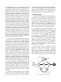
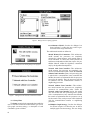
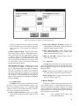
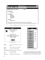
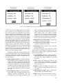
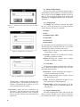
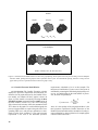
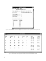
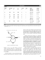
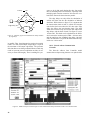
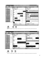
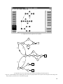
Figure 58. Dataflow analysis of DFG of figure 55 with communication delays and Network without Com Controller model.
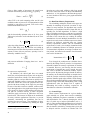
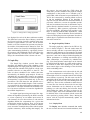
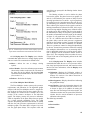
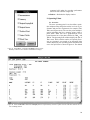
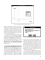
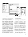
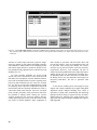
Tool creates a Metrics window for each graph. The first
graph found in the file will be opened along with the
SGP window. All other Metrics windows will be minimized to icons, as shown beside the Parallel Execution
window icon at the bottom of figure 61.
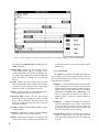
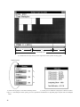
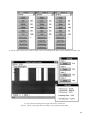
Figure 61 also indicates that Graph 1 requires a fourprocessor schedule for an iteration period of 200 time
units. This is an optimum four-processor solution for
both TBIO and TBO, since there is no idle time in the
periodic schedule. At this level of throughput (1/TBO),
three data sets would execute simultaneously in the
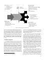
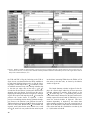
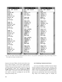
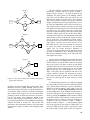
graph. Figure 62 shows the Metrics window, SGP window, and TGP window of Graph 2; eight processors are
required at an iteration period of 108 time units. The
TGP shows that five data sets would be processed in the
graph simultaneously at this level of throughput. The
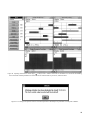
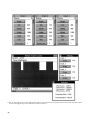
dataflow analysis of Graph 3, portrayed in figure 63,
indicates that four processors would suffice for an iteration period of 134 time units. Since the dataflow schedules of Graph 2 and Graph 3 have idle time, the solutions
are not optimal. Nonetheless, a search for a better solution will not be shown here, since the intent of this discussion is to demonstrate the multiple graph analysis
features.
44
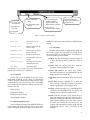
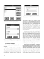
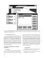
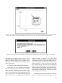
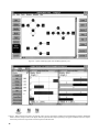
Given the individual scheduling solutions portrayed
in figures 61 to 63, the overall processor requirements
and utilization are displayed by the Parallel Graph Execution window in figure 64. The total computing effort is
computed as 1950 time units by summing the TCE values for all graphs. For each individual graph, the processor requirement is equal to the peak of the corresponding
TRE curve and processor utilization is calculated from
equation (7). To provide for the worst-case overlap of the
individual TRE’s, the total processor requirement is the
sum of the individual processor requirements, calculated
to be 16 in this example. As defined in section 6.4, the
total processor utilization of the system is calculated
from equation (9), where the individual graph speedup
values are summed together and divided by the total
number of processors. In this example, utilization of all
processors is computed to be (800/200 + 750/108 + 400/
134)/16 = 87.1 percent.
10.3.2. Time Multiplex Execution of Multiple
Graphs
This section demonstrates the idea of deterministically controlling the phasing between graphs, which can
produce scheduling solutions with fewer processors. The