Download SAVA User Manual - Christian-Albrechts

SAVA
User Manual
© Christian-Albrechts-Universität Kiel (Germany) and
Technische Universität Bergakademie Freiberg TUBAF (Germany)
Version 1.0
November 22, 2014
1
Authors
The DENISE code was first developed by Daniel Köhn, Olaf Hellwig and Denise De Nil at the Christian-AlbrechtsUniversität Kiel and TU Bergakademie Freiberg (Germany) from January to February 2012.
The anisotropic forward code is an extension of the 3D isotropic elastic FD code fd3D by Olaf Hellwig.
Different external libraries for timedomain filtering are used.
The copyright of the source codes are held by different persons:
cseife.c, cseife.h, lib_stfinv, lib_aff, lib_fourier:
Copyright (c) 2005 by Thomas Forbriger (BFO Schiltach)
cseife_deriv.c, cseife_gauss.c, cseife_rekfl.c, cseife_rfk.c and cseife_tides.c:
Copyright (c) 1984 by Erhard Wielandt
This algorithm was part of seife.f. A current version of seife.f can be obtained from http://www.software-for-seismometry.de/
The Matlab implementation of a few SU routines, mainly used to read and write SU files in data pre-processing
are:
Copyright (C) 2008, Signal Analysis and Imaging Group
For more information: http://www-geo.phys.ualberta.ca/saig/SeismicLab
Author: M.D.Sacchi
Since then it has been developed and maintained by a development team: in alphabetical order,
Maik Linke (TU Bergakademie Freiberg),
(add other developers here in the future).
Contents
1
Introduction
1.1 Citation . . . . . . . . . . . . . . . . . . . . . . . . . . . . . . . . . . . . . . . . . . . . . . . . . .
1.2 Support . . . . . . . . . . . . . . . . . . . . . . . . . . . . . . . . . . . . . . . . . . . . . . . . . .
2
Theoretical Background
2.1 Equations of motion for an elastic medium . . . . . . . .
2.2 Solution of the elastic wave equation by finite differences
2.2.1 Discretization of the equations of motion . . . .
2.2.2 Accuracy of FD operators . . . . . . . . . . . .
2.2.3 Initial and Boundary Conditions . . . . . . . . .
2.3 Numerical Artefacts and Instabilities . . . . . . . . . . .
2.3.1 Grid Dispersion . . . . . . . . . . . . . . . . . .
2.3.2 The Courant Instability . . . . . . . . . . . . . .
.
.
.
.
.
.
.
.
.
.
.
.
.
.
.
.
.
.
.
.
.
.
.
.
.
.
.
.
.
.
.
.
.
.
.
.
.
.
.
.
.
.
.
.
.
.
.
.
.
.
.
.
.
.
.
.
.
.
.
.
.
.
.
.
.
.
.
.
.
.
.
.
.
.
.
.
.
.
.
.
.
.
.
.
.
.
.
.
.
.
.
.
.
.
.
.
.
.
.
.
.
.
.
.
.
.
.
.
.
.
.
.
.
.
.
.
.
.
.
.
.
.
.
.
.
.
.
.
.
.
.
.
.
.
.
.
.
.
.
.
.
.
.
.
.
.
.
.
.
.
.
.
.
.
.
.
.
.
.
.
.
.
.
.
.
.
.
.
.
.
.
.
.
.
.
.
.
.
.
.
.
.
.
.
.
.
.
.
.
.
.
.
6
6
7
7
10
11
14
14
17
The adjoint problem
3.1 What is an ”optimum” model ? . . . . .
3.2 How to find an optimum model . . . . .
∂E
3.3 Calculation of the gradient direction ∂m
3.4 Estimation of an optimum step length µn
3.5 Nonlinear Conjugate Gradient Method .
3.6 The elastic FWT algorithm . . . . . . .
.
.
.
.
.
.
.
.
.
.
.
.
.
.
.
.
.
.
.
.
.
.
.
.
.
.
.
.
.
.
.
.
.
.
.
.
.
.
.
.
.
.
.
.
.
.
.
.
.
.
.
.
.
.
.
.
.
.
.
.
.
.
.
.
.
.
.
.
.
.
.
.
.
.
.
.
.
.
.
.
.
.
.
.
.
.
.
.
.
.
.
.
.
.
.
.
.
.
.
.
.
.
.
.
.
.
.
.
.
.
.
.
.
.
.
.
.
.
.
.
.
.
.
.
.
.
.
.
.
.
.
.
.
.
.
.
.
.
.
.
.
.
.
.
19
19
20
21
26
28
31
3
.
.
.
.
.
.
.
.
.
.
.
.
.
.
.
.
.
.
.
.
.
.
.
.
.
.
.
.
.
.
.
.
.
.
.
.
.
.
.
.
.
.
.
.
.
.
.
.
.
.
.
.
.
.
4
Source Wavelet Inversion
5
Getting Started
5.1 Requirements . . . . . . . . . . . . . . . . . . . . . . . . . .
5.1.1 LAM . . . . . . . . . . . . . . . . . . . . . . . . . .
5.1.2 How to run SAVA on the NEC-Linuxcluster at RZ Kiel
5.2 Installation . . . . . . . . . . . . . . . . . . . . . . . . . . .
5.3 Compilation of SAVA . . . . . . . . . . . . . . . . . . . . . .
5.4 Running the program . . . . . . . . . . . . . . . . . . . . . .
5.5 Postprocessing . . . . . . . . . . . . . . . . . . . . . . . . .
3
4
4
32
.
.
.
.
.
.
.
34
34
34
35
36
37
38
40
6
Definition of parameters for the modelling and inversion code
6.1 Input file with fixed parameters SAVA.inp . . . . . . . . . . . . . . . . . . . . . . . . . . . . . . . .
6.2 Workflow file with variable inversion parameters FWI_workflow.inp . . . . . . . . . . . . . . . . . .
41
41
54
7
Example 1 - coming soon ...
57
.
.
.
.
.
.
.
.
.
.
.
.
.
.
.
.
.
.
.
.
.
.
.
.
.
.
.
.
.
.
.
.
.
.
.
A Harmonic and arithmetic averages of elastic and strain tensor components
2
.
.
.
.
.
.
.
.
.
.
.
.
.
.
.
.
.
.
.
.
.
.
.
.
.
.
.
.
.
.
.
.
.
.
.
.
.
.
.
.
.
.
.
.
.
.
.
.
.
.
.
.
.
.
.
.
.
.
.
.
.
.
.
.
.
.
.
.
.
.
.
.
.
.
.
.
.
.
.
.
.
.
.
.
.
.
.
.
.
.
.
.
.
.
.
.
.
.
.
.
.
.
.
.
.
61
Chapter 1
Introduction
The aim of Full Waveform Tomography (FWT) is to estimate the elastic material parameters in the underground. This
can be achieved by minimizing the misfit energy between the modelled and field data using a gradient optimization
approach. Because the FWT uses the full information content of each seismogram, structures below the seismic wavelength can be resolved. This is a tremendous improvement in resolution compared to traveltime tomography (Pratt
et al. [2002]).
The concept of full waveform tomography was originally developed by Albert Tarantola in the 1980s for the acoustic,
isotropic elastic, and viscoelastic case (Tarantola [1984b,a, 1986, 1988]). First numerical implementations were realized at the end of the 1980s (Gauthier et al. [1986], Mora [1987], Pica et al. [1990]), but due to limited computational
resources, the application was restricted to simple 2D synthetic test problems and small near offset datasets. At the
begining of the 1990s the original time domain formulation was transfered to a robust frequency domain approach
(Pratt and Worthington [1990], Pratt [1990]). With the increasing performance of supercomputers moderately sized
problems could be inverted with frequency domain approaches.
A spectacular result to prove the application of acoustic FWT on laboratory scale was presented by Pratt [1999] for
ultrasonic tomography measurements on a simple block model. In a numerical blind test Brenders and Pratt [2007]
achieved a very good agreement between their inversion result and the unkown true P-wave velocity model. The parallelization and performance optimizations of the frequency domain approach (see e.g. Sourbier et al. [2009a], Sourbier
et al. [2009b]) lead to a wide range of acoustic FWT applications for problems on different scales, from the global
scale, crustal scale over engineering and near surface scale, down to laboratory scale (Pratt [2004]).
Beside the application to geophysical problems, the acoustic FWT is also used to improve the resolution in medical
cancer diagnostics (Pratt et al. [2007]). However, all these examples are restricted to the inversion of the acoustic
material parameters: P-wave velocity, density and additionally the viscoacoustic damping Qp for the P-waves. Even
today the independent 2D FWT of all three isotropic elastic material parameters is still a challenge. Most elastic approaches invert for P-wave velocity only and use empirical relationships to deduce the distribution of S-wave velocity
and density (Shipp and Singh [2002], Sheen et al. [2006]). Recently some authors also investigated the independent
multiparameter FWT in the frequency domain (Choi et al. [2008a,b], Brossier [2009]).
In order to extract information about the structure and composition of the crust from seismic observations, it is
necessary to be able to predict how seismic wavefields are affected by complex structures. Since exact analytical
solutions to the wave equations do not exist for most subsurface configurations, the solutions can be obtained only
by numerical methods. For iterative calculations of synthetic seismograms with limited computer resources fast and
accurate modelling methods are needed.
The FD modelling/inversion program SAVA, is based on the FD approach described by Virieux [1986] and Levander [1988]. The present program SAVA has the following extensions
• considers propagation of seismic waves in general anisotropic elastic media
• is efficently parallelized using domain decomposition with MPI,
• applies Convolutional Perfectly Matched Layer boundary conditions at the edges of the numerical mesh Komatitsch and Martin [2007].
3
CHAPTER 1. INTRODUCTION
4
In the following sections, we give an extensive description of the theoretical background, the different input parameters and show a few benchmark modelling and inversion applications.
1.1
Citation
If you use this code for your own research, please cite at least one article written by the developers of the package, for
instance:
XX
or
(XX add more references here)
and/or other articles from (http://www.geophysik.uni-kiel.de/~dkoehn/publications.htm)
The corresponding BibTEX entries may be found in file doc/USER_MANUAL/thesis.bib.
1.2
Support
The development of the code was suppported by the Christian-Albrechts-Universität Kiel, TU Bergakademie Freiberg,
Deutsche Forschungsgemeinschaft (DFG), Bundesministerium für Bildung und Forschung (BMBF). The code was
tested and optimized at the computing centres of Kiel University, TU Bergakademie Freiberg and the Hochleistungsrechenzentrum Nord (HLRN 1+2).
Acknowledgments and contact
We thank for constructive discussions and further code improvements:
Wolfgang Rabbel (Christian-Albrechts-Universität Kiel).
Please e-mail your feedback, questions, comments, and suggestions to
Daniel Köhn (dkoehn-AT-geophysik.uni-kiel.de).
5
Chapter 2
Theoretical Background
2.1
Equations of motion for an elastic medium
The propagation of waves in a general elastic medium can be described by a system of coupled linear partial differential
equations. They consist of the equations of motion
ρ
∂vi ∂σij
=
+ fi
∂t
∂xj
(2.1)
which simply state that the momentum of the medium, the product of density ρ and the displacement velocity vi , can
be changed by surface forces, described by the stress tensor σij or body forces fi . These equations describe a general
medium, like gas, fluid, solid or plasma. The material specific properties are introduced by additional equations which
describe how the medium reacts when a certain force is applied. In the general anisotropic elastic case this can be
described by a linear stress-strain relationship:
σij = cijkl kl + Tij
1 ∂ui
∂uj
+
ij =
2 ∂xj
∂xi
(2.2)
where cijkl denotes the elastic tensor, ij the strain tensor, Tij surface force source term and ui the displacement vector.
i
Using the definition of the particle velocity vi = ∂u
∂t , (2.1) and (2.2) can be transformed into a system of second order
partial differential equations:
ρ
∂ 2 ui ∂σij
=
+ fi
∂t2
∂xj
σij = cijkl kl + Tij
∂uj
1 ∂ui
+
ij =
2 ∂xj
∂xi
(2.3)
This expression is called Stress-Displacement formulation. Another common form of the elastic equations of motion
can be deduced by taking the time derivative of the stress-strain relationship and the strain tensor in Eq. (2.3). Since
the elastic tensor cijkl does not depend on time, Eq. (2.3) can be written as:
∂vi ∂σij
=
+ fi
∂t
∂xj
∂σij
∂kl
∂Tij
= cijkl
+
∂t
∂t
∂t
∂ij 1 ∂vi
∂vj
=
+
∂t
2 ∂xj
∂xi
ρ
(2.4)
(2.5)
(2.6)
This expression is called Stress-Velocity formulation. For simple cases (2.3) and (2.4) can be solved analytically.
More complex problems require numerical solutions. One possible approach for a numerical solution is described in
the next section.
6
CHAPTER 2. THEORETICAL BACKGROUND
7
(i, j+0.5, k)
vy, <ρ>y
vz, <ρ>z
vx, <ρ>x
(i, j, k)
(i+0.5, j, k)
σxy
σyz
σxz
σxx, σyy, σzz, cijkl, ρ
(i, j, k+0.5)
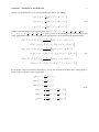
Figure 2.1: Elementary cell for the staggered grid scheme in Cartesian coordinates.
2.2
2.2.1
Solution of the elastic wave equation by finite differences
Discretization of the equations of motion
For the numerical solution the elastic equations of motion (2.4)-(2.6) are discretized in time and space on an equidistant
grid. The particle velocities vi , the stresses σij and components of the elastic tensor cijkl are defined at discrete
Cartesian coordinates x = i dh, y = j dh, z = k dh and discrete times t = n dt. dh denotes the spatial distance
between two adjacent grid points and dt the difference between two successive time steps. Therefore every grid point
is located in the interval i ∈ N|[1, NX], j ∈ N|[1, NY], k ∈ N|[1, NZ] and n ∈ N|[1, NT], where NX, NY, NZ and
NT are the maximum number of discrete spatial grid points in each direction and time steps, respectively. Finally the
partial and temporal derivatives are replaced by 2nd order finite-difference (FD) operators. Two types of operators can
be distinguished, forward and backward operators D+ , D− . The derivative of a function f(x, y, z) with respect to the
x-direction can be approximated by the following operators:
f[k, j, i + 1] − f[k, j, i]
dh
f[k,
j,
i]
−
f[k, j, i − 1]
D−
x f(x, y, z)=
dh
D+
x f(x, y, z)=
forward operator
(2.7)
backward operator
To calculate the spatial derivatives of the wavefield variables at the correct positions and avoid consequent numerical
instabilities, the wavefield variables and model parameters are not placed on the same grid points, but staggered by
half of the spatial grid point distance [Virieux, 1986, Levander, 1988]. Fig. 2.1 shows the distribution of the material
parameters and wavefield variables on the spatial grid. Forward and backward FD operators are choosen according to
the positions of the wavefields on the LHS of eq. (2.4) and (2.5), respectively. For the discretization of the momentum
CHAPTER 2. THEORETICAL BACKGROUND
8
equation (??) the densities have to be averaged arithmetically (Moczo et al. [2004])
1
+ +
+ + +
+ + −
< ρ[k , j , i] >x =
ρ[k , j , i ] + ρ[k , j , i ]
2
1
+
+
+ + +
+ − +
< ρ[k , j, i ] >y =
ρ[k , j , i ] + ρ[k , j , i ]
2
1
+ +
+ + +
− + +
< ρ[k, j , i ] >z =
ρ[k , j , i ] + ρ[k , j , i ]
2
(2.8)
Similiar to Levander [1988] we introduced the abbreviation (i+ , j+ , k+ , n+ ) = (i + 12 , j + 12 , k + 12 , n + 12 ) and
(i− , j− , k− , n− ) = (i − 12 , j − 12 , k − 12 , n − 12 ) to denote positions on the half-staggered spatial and temporal grid
points. Applying these rules to eq. (2.4) leads to the following pseudo code for the discrete momentum equation
dt
n + +
n−1 + +
n− + + −
vx [k , j , i]= vx [k , j , i] +
σ n− [k+ , j+ , i+ ] − σxx
[k , j , i ]
dh < ρ >x xx
n− +
n− +
n−
+
n−
+
+σxy [k , j + 1, i] − σxy [k , j, i] + σxz [k + 1, j , i] − σxz [k, j , i]
dt
n− +
n− +
n +
+
n−1 +
+
σxy
[k , j, i + 1] − σxy
[k , j, i]
vy [k , j, i ]= vy [k , j, i ] +
dh < ρ >y
(2.9)
n− + + +
n− + − +
n−
+
n−
+
+σyy [k , j , i ] − σyy [k , j , i ] + σyz [k + 1, j, i ] − σyz [k, j, i ]
dt
n
+ +
n−1
+ +
n−
vz [k, j , i ]= vz [k, j , i ] +
σ n− [k, j+ , i + 1] − σxz
[k, j+ , i]
dh < ρ >z xz
n−
+
n−
+
n− + + +
n− − + +
+σyz [k, j + 1, i ] − σyz [k, j, i ] + σzz [k , j , i ] − σzz [k , j , i ] .
For the update of the stress-strainrate relationship eq. (2.5) we first discretize the strainrate tensor at the positions of
the stress tensor components on the staggered grid
˙xx [k+ , j+ , i+ ]=
˙yy [k+ , j+ , i+ ]=
˙zz [k+ , j+ , i+ ]=
˙yz [k, j, i+ ]=
˙xz [k, j+ , i]=
˙xy [k+ , j, i]=
∂vx + + +
[k , j , i ]
∂x
∂vy + + +
[k , j , i ]
∂y
∂vz + + +
[k , j , i ]
∂z
1 ∂vy
∂vz
[k, j, i+ ] +
[k, j, i+ ]
2 ∂z
∂y
1 ∂vz
∂vx
[k, j+ , i] +
[k, j+ , i]
2 ∂x
∂z
1 ∂vx +
∂vy +
[k , j, i] +
[k , j, i]
2 ∂y
∂x
(2.10)
CHAPTER 2. THEORETICAL BACKGROUND
9
with the FD operators
∂vx + + +
[k , j , i ]≈ (vx [k+ , j+ , i + 1] − vx [k+ , j+ , i])/dh
∂x
∂vy + + +
[k , j , i ]≈ (vy [k+ , j + 1, i+ ] − vy [k+ , j, i+ ])/dh
∂y
∂vz + + +
[k , j , i ]≈ (vz [k + 1, j+ , i+ ] − vz [k, j+ , i+ ])/dh
∂z
∂vx +
[k , j, i]≈ (vx [k+ , j+ , i] − vx [k+ , j− , i])/dh
∂y
∂vy +
[k , j, i]≈ (vy [k+ , j, i+ ] − vy [k+ , j, i− ])/dh
∂x
∂vz
[k, j+ , i]≈ (vz [k, j+ , i+ ] − vz [k, j+ , i− ])/dh
∂x
∂vx
[k, j+ , i]≈ (vx [k+ , j+ , i] − vx [k− , j+ , i])/dh
∂z
∂vy
[k, j, i+ ]≈ (vy [k+ , j, i+ ] − vy [k− , j, i+ ])/dh
∂z
∂vz
[k, j, i+ ]≈ (vz [k, j+ , i+ ] − vz [k, j− , i+ ])/dh
∂y
(2.11)
Substitution of these expressions in the stress-strain-rate relationship eq. (2.5) for the general anisotropic case leads to
n+ + + +
n− + + +
σxx
[k , j , i ]= σxx
[k , j , i ] + dt ˙nxx c11 + ˙nyy c12 + ˙nzz c13
+ + +
a,n + + +
a,n + + +
+2(˙a,n
xy [k , j , i ]c16 + ˙xz [k , j , i ]c15 + ˙yz [k , j , i ]c14 )
n+ + + +
n− + + +
σyy
[k , j , i ]= σyy
[k , j , i ] + dt ˙nxx c12 + ˙nyy c22 + ˙nzz c23
(2.12)
+ + +
a,n + + +
a,n + + +
+2(˙a,n
xy [k , j , i ]c62 + ˙xz [k , j , i ]c52 + ˙yz [k , j , i ]c24 )
n+ + + +
n− + + +
σzz
[k , j , i ]= σzz
[k , j , i ] + dt ˙nxx c13 + ˙nyy c23 + ˙nzz c33
+ + +
a,n + + +
a,n + + +
+2(˙a,n
xy [k , j , i ]c63 + ˙xz [k , j , i ]c53 + ˙yz [k , j , i ]c43 )
n+ +
n− +
+
h
+
a,n +
h
+
a,n +
h
+
σxy
[k , j, i]= σxy
[k , j, i] + dt ˙a,n
xx [k , j, i]c16 [k , j, i] + ˙yy [k , j, i]c62 [k , j, i] + ˙zz [k , j, i]c63 [k , j, i]
+
h
+
a,n +
h
+
+2(˙nxy [k+ , j, i]ch66 [k+ , j, i] + ˙a,n
xz [k , j, i]c65 [k , j, i] + ˙yz [k , j, i]c64 [k , j, i])
n+
n−
+
h
+
a,n
+
h
+
a,n
+
h
+
σxz
[k, j+ , i]= σxz
[k, j+ , i] + dt ˙a,n
xx [k, j , i]c15 [k, j , i] + ˙yy [k, j , i]c52 [k, j , i] + ˙zz [k, j , i]c53 [k, j , i]
+
h
+
n
+
h
+
a,n
+
h
+
+2(˙a,n
xy [k, j , i]c65 [k, j , i] + ˙xz [k, j , i]c55 [k, j , i] + ˙yz [k, j , i]c54 [k, j , i])
n+
n−
+ h
+
a,n
+ h
+
a,n
+ h
+
σyz
[k, j, i+ ]= σyz
[k, j, i+ ] + dt ˙a,n
xx [k, j, i ]c14 [k, j, i ] + ˙yy [k, j, i ]c24 [k, j, i ] + ˙zz [k, j, i ]c43 [k, j, i ]
+ h
+
a,n
+ h
+
n
+ h
+
+2(˙a,n
xy [k, j, i ]c64 [k, j, i ] + ˙xz [k, j, i ]c54 [k, j, i ] + ˙yz [k, j, i ]c44 [k, j, i ])
(2.13)
To simplify the expression of the elastic tensor we introduced the Voigt notation [Voigt, 1910], where pairs of tensor indices are related to integer numbers from 1 to 6: (1, 1) → 1, (2, 2) → 2, (3, 3) → 3, (2, 3) → 4, (1, 3) → 5,
(1, 2) → 6. The correct update of the stress tensor components on the staggered grid requires the arithmetic averages
of certain strain-rate tensor components ˙aij and the harmonic averages of elastic tensor components chij . The details of
the averaging are described in appendix A. A detailed dispersion and stability analysis for the isotropic case can be
found in Crase [1990], Igel et al. [1995], Saenger et al. [2000], Saenger and Bohlen [2004]. For the general anisotropic
case Igel et al. [1995] suggests to replace the maximum P-wave velocity of the isotropic medium in the stability criterion by the maximum phase velocity in the anisotropic medium. In order to model wave propagtion in an elastic
full- or half-space convolutional PML (C-PML) absorbing boundary conditions are implemented according to the approach by [Komatitsch and Martin, 2007]. To reduce computation time, the resulting code is parallelized by domain
decomposition using MPI.
CHAPTER 2. THEORETICAL BACKGROUND
2.2.2
10
Accuracy of FD operators
The derivation of the FD operators in the last section was a simple replacement of the partial derivatives by finite
differences. In the following more systematic approach, the first derivative of a variable f at a grid point i is estimated
by a Taylor series expansion (Jastram [1992]):
∂f 1
(2k − 1) =
(fi+(k−1/2) − fi−(k−1/2) )
∂x i dh
N
1 X ((k − 21 )dh)2l−1 ∂ (2l−1) f + O(dh)2N
+
(2l−1) dh
(2l − 1)!
∂x
i
l=2
For an operator with length 2N, N equations are added with a weight βk :
N
N
X
∂f 1 X
[
βk (2k − 1)] =
βk (fi+(k−1/2) − fi−(k−1/2) )
∂x i dh
k=1
k=1
N N
1 X X ((k − 21 )dh)2l−1 ∂ (2l−1) f + O(dh)2N
+
βk
dh
(2l − 1)!
∂x(2l−1) i
(2.14)
k=1 l=2
The case N=1 leads to the FD operator derived in the last section, which has a length of 2N=2. The Taylor series is
truncated after the first term (O(dh)2 ). Therefore this operator is called 2nd order FD operator which refers to the
truncation error of the Taylor series and not to the order of the approximated derivative. To understand equation (2.14)
better, we estimate a 4th order FD operator. This operator has the length 2N = 4 or N=2. The sums in Eq. (2.14)
lead to:
∂f 1
(β1 + 3β2 ) =
(β1 (fi+1/2 − fi−1/2 ) + β2 (fi+3/2 − fi−3/2 ))
∂x i dh
(2.15)
dh3
27 ∂ 3 f 1
+
+ β2
β1
dh
8 · 3!
8 · 3! ∂x3 i
The weights βk can be calculated by the following approach: The factor in front of the partial derivative on the LHS
of Eq. (2.15) should equal 1, therefore
(β1 + 3β2 ) = 1.
∂3f The coefficients in front of ∂x
3 on the RHS of Eq. (2.15) should vanish:
i
(β1 + 27β2 ) = 0.
The weights βk can be estimated by solving the matrix equation:
1 3
β1
1
·
=
1 27
β2
0
The resulting coefficients are β1 = 9/8 and β2 = −1/24. Therefore the 4th order backward- and forward operators
are:
∂f 1
=
[β1 (fi+1 − fi ) + β2 (fi+2 − fi−1 )]
forward operator
∂x i+1/2 dh
(2.16)
∂f 1
=
[β
(f
−
f
)
+
β
(f
−
f
)]
backward
operator
1 i
i−1
2 i+1
i−2
∂x dh
i−1/2
The coefficients βi in the FD operator are called Taylor coefficients. The accuracy of higher order FD operators can be
improved by seeking for FD coefficients βk that approximate the first derivative in a certain frequency range (Holberg
[1987]). These numerically optimized coefficients are called Holberg coefficients.
CHAPTER 2. THEORETICAL BACKGROUND
2.2.3
11
Initial and Boundary Conditions
To find a unique solution of the problem, initial and boundary conditions have to be defined. The initial conditions for
the elastic forward problem are:
ui (x, t)= 0
(2.17)
∂ui (x, t)
=0
∂t
for all x ∈ V at t = 0.
For the geophysical application two types of boundary conditions are very important:
1. Horizontal Free Surface: The interface between the elastic medium and air at the surface is very important when
trying to model surface waves or multiple reflections in a marine environment. Since all stresses in the normal
direction at this interface vanish
σxy = σyy = 0.0
(2.18)
this boundary condition is called (stress) free surface. Two types of implementations are common. In the implicit defintion of the free surface, a small layer with the acoustic parameters of air (Vp = 300 m/s, Vs = 0.0 m/s,
ρ = 1.25 kg/m3 ) is placed on top of the model. One advantage of the implicit definition of the free surface is
the easy implementation of topography on the FD grid, however to get accurate results for surface waves or
multiples, this approach requires a fine spatial sampling of the FD grid near the free surface. An explicit free
surface can be implemented by using the mirroring technique by Levander, which leads to stable and accurate
solutions for plain interfaces (Levander [1988], Robertsson et al. [1995]). If the planar free surface is located at
grid point j = h, the stress at this point is set to zero and the stresses below the free surface are mirrored with
an inverse sign:
σyy (h, i)= 0
σyy (h − 1, i)= −σyy (h + 1, i)
1
1
1
σxy (h − , i + )= −σxy (h + , i +
2
2
2
3
1
3
σxy (h − , i + )= −σxy (h + , i +
2
2
2
1
)
2
1
)
2
(2.19)
When updating the stress component σxx = (λ + 2µ)uxx + λuyy at the free surface, only horizontal particle
displacements should be used because vertical derivatives over the free surface lead to instabilities (Levander
[1988]). The vertical derivative of the y-displacement uyy can be replaced by using the boundary condition at
the free surface:
σyy = (λ + 2µ)uyy + λuxx = 0
λ
uxx
uyy = −
(λ + 2µ)
(2.20)
Therefore the stress σxx can be written as
σxx =
4(λµ + µ2 )
uxx
λ + 2µ
(2.21)
2. Absorbing Boundary Conditions: Due to limited computational resources, the FD grid has to be as small as
possible. To model problems with an infinite extension in different directions, e.g. a full or half-space problem,
an artificial absorbing boundary condition has to be applied. A very effective way to damp the waves near the
boundaries are Perfectly Matched Layers (PMLs). This can be achieved by a coordinate stretch of the wave
equations in the frequency domain (Komatitsch and Martin [2007]). The coordinate stretch creates exponentially
decaying plane wave solutions in the absorbing boundary frame. The PML’s are only reflectionless if the exact
wave equation is solved. As soon as the problem is discretized (for example using finite differences) you are
solving an approximate wave equation and the analytical perfection of the PML is no longer valid. To overcome
this shortcoming the wavefield is damped by the damping function
c = −Vpml ∗
log(α)
L
(2.22)
CHAPTER 2. THEORETICAL BACKGROUND
12
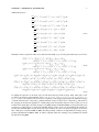
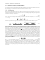
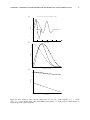
where Vpml denotes the typical P-wave velocity of the medium in the absorbing boundary frame, α = 1 × 10−4
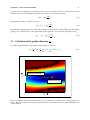
and L is the thickness of the absorbing boundary layer. A comparison between the exponential damping and the
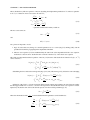
PML boundary is shown in Fig.2.2. The PMLs are damping the seismic waves by a factor 5-10 more effective
than the absorbing boundary frame.
CHAPTER 2. THEORETICAL BACKGROUND
13
Figure 2.2: Comparison between exponential damping (left column) and PML (right column) absorbing boundary
conditions for a homogeneous full space model.
CHAPTER 2. THEORETICAL BACKGROUND
2.3
14
Numerical Artefacts and Instabilities
To avoid numerical artefacts and instabilities during a FD modelling run, spatial and temporal sampling conditions for
the wavefield have to be satisfied. These will be discussed in the following two sections.
2.3.1
Grid Dispersion
The first question when building a FD model is: What is the maximum spatial grid point distance dh, for a correct
sampling of the wavefield ? To answer this question we take a look at this simple example: The particle displacement
in x-direction is defined by a sine function:
x
,
(2.23)
ux = sin 2π
λ
where λ denotes the wavelength. When calculating the derivation of this function analytically at x = 0 and setting
λ = 1 m we get:
dux 2π
x =
= 2π.
(2.24)
cos 2π
dx x=0 λ
λ x=0
In the next step the derivation is approximated numerically by a staggered 2nd order finite-difference operator:
2π(x− 21 dx)
2π(x+ 12 dx)
− sin
sin
λ
λ
ux (x + 12 ∆x) − ux (x − 12 ∆x) dux .
(2.25)
≈
=
dx x=0
∆x
∆x
x=0
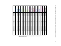
Using the Nyquist-Shannon sampling theorem it should be sufficient to sample the wavefield with ∆x = λ/2. In
table 2.1 the numerical solutions of eq. (2.25) and the analytical solution (2.24) are compared for different sample
intervals ∆x = λ/n, where n is the number of gridpoints per wavelength. For the case n=2, which corresponds to the
x
Nyquist-Shannon theorem, the numerical solution is du
dx |x=0 = 4.0, which is not equal with the analytical solution
2π. A refinement of the spatial sampling of the wavefield results in an improvement of the finite difference solution.
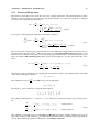
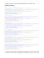
For n = 16 the numerical solution is accurate to the second decimal place. The effect of a sparsly sampled pressure
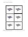
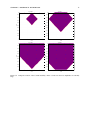
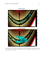
field is illustrated in figure 2.3 for a homogeneous block model with stress free surfaces. The dimensions of the FD
grid are fixed and the central frequency of the source signal is increased systematically. When using a spatial sampling
of 16 grid points per minimum wavelength (figure 2.3, top) the wavefronts are sharply defined. For n = 4 grid points
a slight numerical dispersion of the wave occurs (figure 2.3, center). This effect is obvious when using the Nyquist
criterion (n = 2) (figure 2.3, bottom). Since the numerical calculated wavefield seem to be dispersive this numerical
artefact is called grid dispersion. To avoid the occurence of grid dispersion the following criteria for the spatial grid
spacing dh has to be satisfied:
λmin
Vmin
dh ≤
=
.
(2.26)
n
n fmax
Here λmin denotes the minimum wavelength, Vmin the minimum velocity in the model and fmax is the maximum
frequency of the source signal. Depending on the accuracy of the used FD operator the parameter n is different.
In table 2.2 n is listed for different FD operator lengths and types (Taylor and Holberg operators). The Holberg
coefficients are calculated for a minimum dispersion error of 0.1% at 3fmax . For short operators n should be choosen
relatively large, so the spatial grid spacing is small, while for longer FD operators n is smaller and the grid spacing
can be larger.
CHAPTER 2. THEORETICAL BACKGROUND
n
analytical
2
4
8
16
32
15
∆x [m]
λ/2
λ/4
λ/8
λ/16
λ/32
dvx
dx |x=0
[]
2π ≈ 6.283
4.0
5.657
6.123
6.2429
6.2731
Table 2.1: Comparison of the analytical solution Eq. (2.24) with the numerical solution Eq. (2.25) for different grid
spacings ∆x = λ/n.
FDORDER
2nd
4th
6th
8th
10th
12th
n (Taylor)
12
8
6
5
5
4
n (Holberg)
12
8.32
4.77
3.69
3.19
2.91
Table 2.2: The number of grid points per minimum wavelength n for different orders (2nd-12th) and types (Taylor
and Holberg) of FD operators. For the Holberg coefficients n is calculated for a minimum dispersion error of 0.1% at
3fmax .
500
500
1000
1000
1500
1500
2000
2000
2500
3000
3000
3500
4000
4000
4500
4500
5000
5000
2000
3000
Distance [m]
4000
5000
500
500
1000
1000
1500
1500
2000
2000
Depth [m]
Depth [m]
2500
3500
1000
2500
3000
3500
4000
4500
4500
5000
5000
4000
5000
500
1000
1000
1500
1500
2000
2000
Depth [m]
500
2500
3000
3500
4000
4500
4500
5000
5000
4000
5000
5000
1000
2000
3000
Distance [m]
4000
5000
1000
2000
3000
Distance [m]
4000
5000
3000
4000
2000
3000
Distance [m]
4000
2500
3500
1000
2000
3000
Distance [m]
3000
4000
2000
3000
Distance [m]
1000
2500
3500
1000
Depth [m]
16
Depth [m]
Depth [m]
CHAPTER 2. THEORETICAL BACKGROUND
Figure 2.3: The influence of grid dispersion in FD modelling: Spatial sampling of the wavefield using n=16 (top),
n=4 (center) and n=2 gridpoints (bottom) per minimum wavelength λmin .
CHAPTER 2. THEORETICAL BACKGROUND
2.3.2
17
The Courant Instability
Beside the spatial, the temporal discretization has to satisfy a sampling criterion to ensure the stability of the FD code.
If a wave is propagating on a discrete grid, then the timestep dt has to be less than the time for the wave to travel
between two adjacent grid points with grid spacing dh. For an elastic 2D grid this means mathematically:
dh
dt ≤ √
,
h 2Vmax
(2.27)
where Vmax is the maximum velocity in the model. The factor h depends on the order of the FD operator and can
easily calculated by summing over the weighting coefficients βi
X
h=
βi .
(2.28)
i
In table 2.3 h is listed for different FD operator lengths and types (Taylor and Holberg operators). Criterion (2.27)
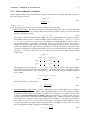
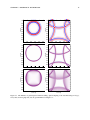
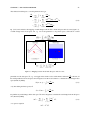
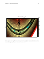
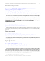
is called Courant-Friedrichs-Lewy criterion (Courant et al. [1928], Courant et al. [March 1967]). figure 2.4 shows
the evolution of the pressure field when the Courant criterion is violated. After a few time steps the amplitudes are
growing to infinity and the calculation becomes unstable.
FDORDER
2nd
4th
6th
8th
10th
12th
h (Taylor)
1.0
7/6
149/120
2161/1680
53089/40320
1187803/887040
h (Holberg)
1.0
1.184614
1.283482
1.345927
1.387660
1.417065
Table 2.3: The factor h in the Courant criterion for different orders (2nd-12th) and types (Taylor and Holberg) of FD
operators.
CHAPTER 2. THEORETICAL BACKGROUND
18
T= 1.5ms
0
0.1
0.1
0.2
0.2
0.3
0.3
0.4
0.4
y/m
y/m
T= 0.8ms
0
0.5
0.5
0.6
0.6
0.7
0.7
0.8
0.8
0.9
0.9
1
0
0.2
0.4
0.6
0.8
1
1
0
0.2
0.4
x/m
0.1
0.1
0.2
0.2
0.3
0.3
0.4
0.4
0.5
0.6
0.7
0.7
0.8
0.8
0.9
0.9
0.2
0.4
0.6
x/m
1
0.6
0.8
1
0.5
0.6
0
0.8
T= 3.0ms
0
y/m
y/m
T= 2.3ms
0
1
0.6
x/m
0.8
1
1
0
0.2
0.4
x/m
Figure 2.4: Temporal evolution of the Courant instability. In the colored areas the wave amplitudes are extremly
large.
Chapter 3
The adjoint problem
The aim of full waveform tomography is to find an ”optimum” model which can explain the data very well. It should
not only explain the first arrivals of specific phases of the seismic wavefield like refractions or reflections, but also the
amplitudes which contain information on the distribution of the elastic material parameters in the underground. To
achieve this goal three problems have to be solved:
1. What is an ”optimum” model ?
2. How can this model be found ?
3. Is this model unique or are other models existing, which could explain the data equally well ?
3.1
What is an ”optimum” model ?
In reflection seismics the ith component of the elastic displacement field ui (xs , xr , t) excited by sources located at xs
will be recorded by receivers at xr at time t. For a given distribution of the material parameters the forward problem
Eq. 2.3 can be solved by finite differences (section 2.2). The result is a model data set umod . This modelled data
can be compared with the field data uobs . If the misfit or data residuals δu = umod − uobs (figure 3.1) between the
modelled and the field data is small the model can explain the data very well. If the residuals are large the model
cannot explain the data. The misfit can be measured by a vector norm |L|p which is defined for p = 1, 2, ... as
|L|p =
X
p
1/p
|δui |
(3.1)
i
The special case |L|∞ is defined as
|L|∞ = maxi |δui |p
The L2-norm
(3.2)
1 T
δu δu
(3.3)
2
has a special physical meaning. It represents the residual elastic energy contained in the data residuals δu. An optimum
model can be found in a minimum of the residual energy. Therefore the optimum model is the solution of a nonlinear
optimization problem.
E = |L|2 =
19
CHAPTER 3. THE ADJOINT PROBLEM
3.2
20
How to find an optimum model
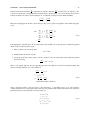
Figure 3.2 shows a schematic sketch of the residual energy at one point in space as a function of two model parameters
λ and µ. The colors represent different values of the residual energy. Red areas represent models with high residual
energy which do not fit the data, while the blue parts are good fitting models with low residual energies. The aim is to
find the minimum of the residual energy marked by the red cross. Starting at a point m1 = (λ1 (x), µ1 (x), ρ1 (x), ) in
the parameter space we want to find the minimum by updating the material parameters in an iterative way
m2 = m1 + µ1 δm1 ,
(3.4)
along the search direction δm1 with the step length µ1 . To find the optimum search direction δm1 we expand the
residual energy E(m1 + δm1 ) near the starting point in a Taylor series:
2 ∂E
1
∂ E
δmT
(3.5)
E(m1 + δm1 ) ≈ E(m1 ) + δm1
+ δm1
∂m 1 2
∂m2 1 1
and set the derivative of Eq. 3.5 with respect to δm1 zero
2 ∂E(m1 + δm1 )
∂ E
∂E
+ δm1
=0
=
∂δm1
∂m 1
∂m2 1
(3.6)
Which finally leads to
δm1 = −
∂2E
∂m2
−1 1
∂E
∂m
= −H1 −1
1
∂E
∂m
(3.7)
1
where (∂E/∂m)1 denotes the steepest-descent direction of the objective function and H1 −1 the inverse Hessian
matrix. The inverse Hessian matrix for the elastic problem is often singular and can only be calculated with high
computational costs. Therefore the inverse Hessian matrix is approximated by a preconditioning operator P. There is
u
−
u
obs
=
δu
¬ time
mod
channel ®
channel ®
Figure 3.1: Definition of data residuals δu.
channel ®
CHAPTER 3. THE ADJOINT PROBLEM
21
no general rule for an optimum preconditioning operator, but two very simple operators are described in more detail
in chapter ?? for a cross-well acquisition geometry and in chapter ?? for a reflection geometry.
∂E
δm1 ≈ −P1
.
(3.8)
∂m 1
By replacing δm1 in Eq. 3.4 with Eq. 3.8 we get
m2 = m1 − µ1 P1
∂E
∂m
,
(3.9)
1
The optimum model parameters can be found along the negative gradient direction of the residual energy. The starting
point m1 is not a particular point, so the update function can be applied to every point in the parameter space mn
∂E
mn+1 = mn − µn Pn
.
(3.10)
∂m n
3.3
Calculation of the gradient direction
∂E
∂m
To estimate the gradient direction ∂E/∂m the residual energy is rewritten as:
Z
X
1
1 X
E = δuT δu =
dt
δu2 (xr , xs , t)
2
2 sources
(3.11)
Starting model m1
2
mµ ®
receiver
Final model m n
mλ1 ®
Figure 3.2: Schematic sketch of the residual energy at one point in space as a function of two model parameters m1
and m2 . The blue dot denotes the starting point in the parameter space, while the red cross marks a minimum of the
objective function.
CHAPTER 3. THE ADJOINT PROBLEM
22
After derivation with respect to a model parameter m we get
X Z
X ∂δu
∂E
=
dt
δu
∂m sources
∂m
receiver
X Z
X ∂(umod (m) − uobs )
=
dt
δu
∂m
sources
receiver
X ∂umod (m)
X Z
dt
=
δu
∂m
sources
(3.12)
receiver
Eq. (3.12) can be related to the mapping of small changes from the data to the model space and vice versa (figure 3.3).
A small change in the model space δm, e.g. one model parameter at one point in space, will result in a small
Figure 3.3: Mapping between model and data space and vice versa.
∂u
perturbation of the data space δũ, e.g. one wiggle in the seismic section. If the Frechét derivative ∂m
is known, all
the small perturbations in model space can be integrated over the model volume V to calculate the total change in data
space (Tarantola [2005]):
Z
∂u
δũ(xs , xr , t) =
dV
δm,
(3.13)
∂m
V
or by introducing the linear operator L̂
Z
δũ = L̂δm :=
dV
V
∂u
δm.
∂m
In a similar way small changes in the data space δũ0 can be integrated to calculate the total change in the model space
δm0 (Tarantola [2005])
X Z
X ∂u ∗
0
δm =
dt
δũ0 ,
(3.14)
∂m
sources
receiver
or as operator equation
δm0 = L̂∗ δũ0 .
CHAPTER 3. THE ADJOINT PROBLEM
23
∗
∂u
∂u
In this case the Frechét derivative ∂m
is replaced by it’s adjoint counterpart ∂m
. Note that δũ 6= δũ0 and δm 6= δm0 ,
so there is no unique way to map perturbations from the model to the data space or vice versa. Because the operator L̂
is linear, the kernel of L̂ and it’s adjoint counterpart L̂∗ are identical (see chapter 5.4.2 in Tarantola [2005])
∗ ∂u
∂u
=
∂m
∂m
Therefore the mapping from the data to the model space Eq. (3.14) is equal to the gradient of the residual energy Eq.
(3.12):
X ∂ui ∗
δũ0
dt
δm =
∂m
sources
receiver
X ∂ui X Z
dt
=
δu
∂m
sources
X Z
0
(3.15)
receiver
∂E
=
∂m
if the perturbation of the data space δũ0 is interpretated as data residuals δu. So the approach to estimate the gradient
direction ∂E/∂m can be split into 3 parts
1. Find a solution to the forward problem
δu = L̂δm.
2. Identify the Frechét kernels ∂u/∂m
3. Use the property, that a linear operator L̂ and it’s adjoint L̂∗ have the same kernels and calculate the gradient
direction by using:
∂E
= δm0 = L̂∗ δu0 .
∂m
This is a very general approach. Now we apply this approach to the equations of motion for an elastic medium. The
elastic forward problem Eqs. (2.3) can be written as
ρ
∂ 2 ui
∂
−
σij = fi ,
∂t2
∂xj
σij −cijkl kl = Tij ,
1 ∂ui
∂uj
ij =
+
,
2 ∂xj
∂xi
(3.16)
+ initial and boundary conditions,
where ρ denotes the density, σij the stress tensor, ij the strain tensor, cijkl the stiffness tensor, fi , Tij source terms for
volume and surface forces, respectively. In the next step every parameter and variable in the elastic wave equation is
perturbated by a first order perturbation as shown in Fig. 3.3:
ui → ui + δui ,
ρ→ ρ + δρ,
σij → σij + δσij ,
cijkl → cijkl + δcijkl ,
ij → ij + δij ,
(3.17)
CHAPTER 3. THE ADJOINT PROBLEM
24
These substitutions yield new equations of motion describing the displacement perturbations δui and stress perturbations δσij as a function of new source terms ∆fi and ∆Tij
ρ
∂
∂ 2 δui
−
δσij = ∆fi ,
2
∂t
∂xj
δσij −cijkl δkl = ∆Tij ,
1 ∂δui
∂δuj
δij =
+
2 ∂xj
∂xi
(3.18)
+ perturbated initial and boundary conditions
The new source terms are
∂ 2 ui
∂t2
(3.19)
∆Tij = δcijkl kl .
(3.20)
∆fi = −δρ
and
Two points are important to notice:
1. Eq.(3.18) states that every change of a material parameter acts as a source (Eq.(3.19) and Eq.(3.20)), but the
perturbated wavefield is propagating in the unperturbated medium.
2. The new wave equation (3.18) has mathematically the same form as the unperturbated elastic wave equation,
and hence its solution can be obtained in terms of Green’s functions Gij of the elastic wave equation.
The solution of the perturbated elastic equations of motion (3.18) in terms of the elastic Green’s function Gij (x, t; x0 , t0 )
can be written as:
Z
Z T
δui (x, t)=
dV
dt0 Gij (x, t; x0 , t0 )∆fj (x0 , t0 )
V
0
(3.21)
Z
Z T
0 ∂Gij
0 0
0 0
−
dV
dt
(x, t; x , t )∆Tjk (x , t ).
∂x0k
V
0
Substituting the force and traction terms given by Eqs.(3.19) and (3.20) into Eq.(3.21) yields after some rearranging
Z
Z T
∂ 2 uj
δui (x, t)= −
dV
dt0 Gij (x, t; x0 , t0 ) 2 (x0 , t0 )δρ
∂t
V
0
(3.22)
Z
Z T
∂G
ij
0
0 0
0 0
−
dV
(x, t; x , t )lm (x , t )δcjklm
dt
∂x0k
V
0
Utilization of Eq.(3.22) to solve the forward problem is known as Born approximation. In waveform tomography
the Born approximation is not used to solve the forward problem. Instead the full elastic wave equation is solved.
Equation (3.22) has the same form as the desired expression for the forward problem Eqs.(3.13):
Z
∂u
δu =
dV
δm.
(3.23)
∂m
V
Therefore the Frechét kernels
∂ui
∂m(x)
for the individual material parameters can be identified as:
∂ui
=−
∂ρ
Z
∂ui
=−
∂cjklm
Z
T
dt0 Gij (x, t; x0 , t0 )
0
0
T
dt0
∂ 2 uj 0 0
(x , t )
∂t2
∂Gij
(x, t; x0 , t0 )lm (x0 , t0 )
∂x0k
(3.24)
CHAPTER 3. THE ADJOINT PROBLEM
25
By definition the adjoint of the operator (3.23) can be written as
∗
rec X
X Z T N
∂ui
0
dt
δm (x) =
δu0i (xα , t0 ),
∂m
sources 0
α=1
(3.25)
Because a linear operator and its transpose have the same kernels ∂ui /∂m, the only difference arise in the variables
of sum/integration, which are complementary. Inserting the integral kernels (3.24) in Eq.(3.25) yields
rec Z T
X
X Z T N
∂ 2 uj
0
dt
dt0 Gij (xα , t0 ; x, t) 2 (x, t)δu0i (xα , t0 ),
δρ = −
∂t
sources 0
α=1 0
rec Z T
X
X Z T N
∂Gij
dt0
dt
(xα , t0 ; x, t)lm (x, t)δu0i (xα , t0 ).
δc0jklm = −
∂x
k
sources 0
α=1 0
The terms only depending on time t and the positions x can be moved infront of the sum over the receivers
N
rec Z T
X
X Z T ∂ 2 uj
dt 2 (x, t)
dt0 Gij (xα , t0 ; x, t)δu0i (xα , t0 ),
δρ0 = −
∂t
sources 0
α=1 0
Z
N
rec
T
X
XZ T
∂Gij
(xα , t0 ; x, t)δu0i (xα , t0 ).
δc0jklm = −
dtlm (x, t)
dt0
∂x
k
0
0
sources
α=1
(3.26)
Defining the wavefield
Ψj (x, t)=
N
rec
X
T
Z
dt0 Gij (xα , t0 ; x, t)δu0i (xα , t0 ),
(3.27)
0
α=1
Eqs.(3.26) can be written as
δρ = −
dt
0
sources
δc0jklm =
T
X Z
0
T
X Z
−
0
sources
∂ 2 uj
Ψj ,
∂t2
∂Ψj
dtlm
.
∂xk
(3.28)
The wavefield Ψj is generated by propagating the residual data δu0i from the receiver positions backwards in time
through the elastic medium. To obtain a more symmetric expression for the gradient δc0jklm we exchange the indices j
and k in Eqs. (3.21) - (3.28) and add both gradient expressions
δc0jklm
+
δc0kjlm =
X Z
−
T
dtlm
0
sources
∂Ψk
∂Ψj
+
.
∂xk
∂xj
(3.29)
Because both gradients should be equal we get
2δc0jklm = −
X Z
sources
δc0jklm = −
with Θjk =
1
2
∂Ψj
∂xk
+
∂Ψk
∂xj
dtlm
0
X Z
sources
T
∂Ψk
∂Ψj
+
.
∂xk
∂xj
(3.30)
T
dtlm Θjk ,
0
. Therefore the gradients for density and components of the elastic tensor are:
δρ0 = −
X Z
sources
δc0jklm =
−
dt
0
X Z
sources
T
0
∂ 2 uj
Ψj ,
∂t2
(3.31)
T
dtlm Θjk ,
CHAPTER 3. THE ADJOINT PROBLEM
3.4
26
Estimation of an optimum step length µn
The choice of the step length µn in Eq. 3.10 is crucial for the convergence of the steepest gradient optimization
method. I demonstrate this using a very familiar test problem for optimization routines, the Rosenbrock function with
two unkown parameters (Rosenbrock [1960], Fig. 3.4)
fr (x, y) = (1 − x)2 + 100(y − x2 )2
(3.32)
The aim is to find the minimum of this function located at the point [1,1] which is surrounded by a very narrow valley.
We start the search for the minimum at [-0.5,0.5]. An obvious first choice would be a constant step length. Fig. 3.4
(top) shows the convergence after 16000 iteration steps of the steepest descent method when choosing a step length
µn = 2e − 3. Note the large model update during the first iteration step, when the gradient of the Rosenbrock function
is large. After reaching the narrow valley the gradient is much smaller and as a result the model updates are also
decreasing. This leads to a very slow convergence speed. Especially near the minimum the model updates become
very small. When choosing a larger step length (µn = 2e − 3, Fig. 3.4 (bottom)) the model update is larger even
when the gradient is small, but the code fails to converge at all. Instead it is trapped in a narrow part of the valley. To
solve this problem a variable step length is introduced. For three test step lengths µ1 , µ2 and µ3 three test models are
calculated
mtest1 = mn + µ1 δm0n
mtest2 = mn + µ2 δm0n
mtest3 = mn +
(3.33)
µ3 δm0n
and the corresponding L2-norms L21 , L22 and L23 are estimated (Fig. 3.5). The true misfit function (yellow line) can
be approximated by fitting a parabola through the three points
L2i = aµ2i + bµi + c
(3.34)
where i ∈ {1, 2, 3} and a, b, c are the unkown coefficients. This system of equations can be written as matrix equation:
 2
 
 

µ1 µ1 1
a
L21
 µ22 µ2 1  ·  b  =  L22 
µ23 µ3 1
c
L23
or
Ax = b.
(3.35)
The unknown coefficients of this matrix equation are formally defined by
x = A−1 b,
(3.36)
In the FWT code the solution vector x is calculated by Gaussian elimination. In the following the step length at the
extremum of the parabola defines the optimum step length µopt (denoted as green square in Fig.3.5). This optimum
step length is
b
(3.37)
µopt = − .
2a
The application of the variable step length calculation to the Rosenbrock test problem is shown in Fig. 3.6. The number
of required iteration steps to reach the minimum is reduced by a factor 80 when compared with the constant step length
gradient method. The only problem remaining is the slow convergence speed in the small valley of the Rosenbrock
function, due to the fact that the update occurs along the gradient direction of the objective function resulting in a
”criss-cross” pattern. This behaviour can be avoided by applying a nonlinear conjugate gradient method (chapter 3.5).
In case of the FWT algorithm the three test step lengths for the individual material parameter classes are calculated by
scaling the maximum of the gradient to the maximum of the actual models:
max(λn )
max(δλn )
max(µn )
µµ = p
max(δµn )
max(ρn )
µρ = p
srho
max(δρn )
µλ = p
(3.38)
CHAPTER 3. THE ADJOINT PROBLEM
27
Residual Energy E
250
200
y→
150
100
50
x→
Residual Energy E
250
200
y→
150
100
50
x→
Figure 3.4: Results of the convergence test for the Rosenbrock function. The minimum is marked with a red point, the
starting position with a blue point. The maximum number of iterations is 16000. The step length µn varies between
2e − 3 (top) and 6.1e − 3 (bottom).
CHAPTER 3. THE ADJOINT PROBLEM
28
Normalized L2−Norm
Case 1
( µ , L2 )
1 1
minimum of the parabolic fit
= optimum step length
( µ , L2 )
2
2
( µ , L2 )
3
3
Step length µ
Figure 3.5: Line search algorithm to find the optimum step length µopt : The true misfit function (yellow line) is
approximated by a parabola fitting values of the objective function for 3 different step length.
Because changes of the density model are in most cases smaller than velocity changes the step length for the density
update can be systematically reduced by a factor srho . All material parameters can be updated simultaneously or according to a hierachical strategy. To save computational time the corresponding L2 −norms are calculated for a few
representative shots. The number of shots depends on the complexity of the problem and the signal/noise ratio of the
data. For the acoustic case the step length estimation by parabolic fitting works very well and leads to a smooth decrease of the misfit function during the FWT (Kurzmann (2007), personal communication, ?). For the multiparameter
elastic FWT the misfit function consists of more local minima and therefore the decrease of the objective function is
not as smooth as in the acoustic case. Brossier [2009] proposed a more intensive bracketing stage before applying the
parabolic fit. Starting from p1 = 0.0 the test step lengths p2 and p3 are calculated to satisfy the following criteria:
L22 (mtest2 = mn + µ2 δm0n ) < L21 (mtest1 = mn )
L23 (mtest3 = mn + µ3 δm0n ) > L22 (mtest2 = mn + µ2 δm0n )
(3.39)
This approach leads to a smoother decrease of the objective function, but also increases the number of required forward
models.
3.5
Nonlinear Conjugate Gradient Method
To increase the convergence speed in narrow valleys it would be better to update the model at iteration step n not
exactly along the gradient direction δmn , but along the conjugate direction δcn
δcn = δmn + βn δcn−1 ,
(3.40)
The first iteration step (n=1) consists of a model update along the steepest descent direction:
m2 = m1 + µ1 δm1 ,
(3.41)
For all subsequent iteration steps (n > 1) the model is updated along the conjugate direction:
mn+1 = mn + µn δcn ,
where δc1 = δm1 . The weighting factor β can be calculated in different ways [Nocedal and Wright, 2006]:
(3.42)
CHAPTER 3. THE ADJOINT PROBLEM
29
Residual Energy E
250
200
y→
150
100
50
x→
Figure 3.6: Results of the convergence test for the Rosenbrock function using the pure gradient method. The minimum
is marked by a red point, the starting position by a blue point. The number of iterations is 200. The optimum step
length is calculated at each iteration by the parabola fitting algorithm. Note the criss-cross pattern of the updates in
the narrow valley and the slow convergence speed near the minimum.
1. Fletcher-Reeves [Fletcher and Reeves, 1964]:
δmT
n δmn
δmT
n−1 δmn−1
(3.43)
δmT
n (δmn − δmn−1 )
δmT
n−1 δmn−1
(3.44)
δmT
n (δmn − δmn−1 )
δcT
n−1 (δmn − δmn−1 )
(3.45)
βnFR =
2. Polak-Ribiére [Polak and Ribière, 1969]:
βnPR =
3. Hestenes-Stiefel [Hestenes and Stiefel, 1952]:
βnHS =
We use the very popular choice βn = max[0, βnPR ] which provides an automatic direction reset. This is important
because subsequent search directions lose conjugacy requiring the search direction to be reset to the steepest descent
direction. Note that the conjugate gradient method doesn’t require any additional computational time because only
the gradient δmn at two subsequent iterations has to be known. The application of the nonlinear conjugate gradient
method combined with the variable step length calculation to the Rosenbrock function is shown in Fig. 3.7. The
criss-cross pattern of the steepest descent method has vanished and the conjugate gradient method already converges
after 30 iterations compared with 200 iteration steps of the pure gradient method.
CHAPTER 3. THE ADJOINT PROBLEM
30
Residual Energy E
250
200
y→
150
100
50
x→
Figure 3.7: Results of the convergence test for the Rosenbrock function using the nonlinear conjugate gradient method,
where the optimum step length is calculated with the parabolic fitting algorithm. The minimum is marked by a red
cross, the starting point by a blue point. The number of iterations is 30.
CHAPTER 3. THE ADJOINT PROBLEM
3.6
31
The elastic FWT algorithm
In summary the FWT algorithm consists of the following steps:
1. Define a starting model m1 in the parameter space. This model should represent the long wavelength part of the
underground very well, because the FWT code is only capable to reconstruct structures at or below the dominant
seismic wavelength due to its slow convergence speed, the nonlinearity of the problem and the inherent use of
the Born approximation to calculate the gradient direction.
2. At iteration step n do:
(a) For each shot solve the forward problem, stated in Eq.(3.16) for the actual model mn to generate a synthetic
dataset umod and the wavefield u(x, t).
(b) Calculate the residual seismograms δu = umod − uobs for the x- and y-components of the seismic data.
(c) Generate the wavefield Ψ(x, t) by backpropagating the residuals from the receiver postions.
(d) Calculate the gradients δmn of each material parameter according to Eqs.(??).
(e) To increase the convergence speed an appropriate preconditioning operator P is applied to the gradient δm
δmpn = Pδmn
(3.46)
Examples of simple preconditioning operator are given in chapter ?? for a cross-well acquisition geometry
and in chapter ?? for a reflection geometry.
(f) For a further increase of the convergence speed calculate the conjugate gradient direction for iteration steps
n ≥ 2:
δcn = δmpn + βδcn−1 , with δc1 = δmp1
(3.47)
where the weighting factor
β PR = δmpn
δmpn − δmpn−1
δmpn−1 δmpn−1
(3.48)
by Polak-Ribiére is used. The convergence of the Polak-Ribiére method is guaranteed by choosing β = max[β PR , 0].
(g) Estimate the step length µn by the line search algorithm described in chapter 3.4.
(h) Update the material parameters using the gradient method
mn+1 = mn − µn δcn .
(3.49)
If the material parameters are not coupled by empirical relationships it is important to update all three
elastic material parameters at the same time, otherwise strong artefacts may dominate the inversion result,
especially in the case of very complex media.
3. If the residual energy E is smaller than a given value stop the iteration. Otherwise continue with the next iteration
step.
Chapter 4
Source Wavelet Inversion
So far we assumed that only the material parameters are unkown, while the characteristics of the sources are perfectly
known. For the application of FWI to a field dataset the source wavelet has to be estimated. In frequency domain the
source wavelet s has the complex value
s = e + if
√
where i = −1, e and f are the real and imaginary parts, respectively. The seismograms of the vertical displacements
of the modelled data can be described by:
vrm = (cv,r + idv,r )(e + if)
where (cv,r + idv,r ) denotes the spike response of the vertical displacement and r the receiver location. Similar the
seismograms of the vertical displacements of the field data are:
vrd = (av,r + ibv,r )
Update the real and imaginary parts of the source wavelet with the Newton method
∂E
en+1 = en − Hn −1
,
∂e n
(4.1)
∂E
fn+1 = fn − Hn −1
.
∂f n
∂E
where H, ∂E
∂e n and ∂f n are the Hessian matrix and gradient vector for e and f, respectively. With the objective
function
1X m
E=
(v − vrd )(vrm − vrd )∗
(4.2)
2 r r
the gradients and Hessian can be explictly calculated
∂E X
=
[e(c2v,r + d2v,r ) − av,r cv,r − bv,r dv,r ]
∂e
r
∂E X 2
=
[f(cv,r + d2v,r ) + av,r dv,r − bv,r cv,r ]
∂f
r
∂2E X 2
=
(cv,r + d2v,r ),
∂e2
r
∂2E
∂2E
= 0,
= 0,
∂f∂e
∂e∂f
∂2E X 2
=
(cv,r + d2v,r ).
∂f 2
r
32
(4.3)
CHAPTER 4. SOURCE WAVELET INVERSION
33
Inserting Eq. (4.3) in Eq. (4.1) leads to
P
en+1 =
c
r (a
Pv,r v,r
2
r (cv,r
− bv,r dv,r )
+ d2v,r )
P
fn+1 = −
d − bv,r cv,r )
r (a
Pv,r 2v,r
.
2
r (cv,r + dv,r )
(4.4)
To stabilize the inversion a Marquardt-Levenberg regularization is required:
−1 ∂E
en+1 = en − (Hn + λe I)
∂e n
∂E
−1
fn+1 = fn − (Hn + λf I)
∂f n
where λe , λf are damping factors and I the unity matrix. Therefore Eq. (4.4) can be written as
P
(av,r cv,r − bv,r dv,r )
en+1 = Pr 2
(cv,r + d2v,r ) + λe
Pr
(av,r dv,r − bv,r cv,r )
.
fn+1 = − Pr 2
2
r (cv,r + dv,r ) + λf
The values of the damping factors can be expressed as fractions of the maximum value in the denominators
X
λe = λf = stf max (c2v,r + d2v,r )
r
This approach is a stabilized Wiener deconvolution.
(4.5)
(4.6)
Chapter 5
Getting Started
In the following sections, we give a short description of the different modelling parameters, options and how the
program is used in a parallel MPI environment.
5.1
Requirements
The parallelization employs functions of the Message Passing Interface (MPI). MPI has to be installed when compiling
and running the SAVA software. At least two implementations exist for Unix-based networks: OpenMPI, MPICH2 and
Intel-MPI. The LAM-MPI implementation is no longer supported by the developers. Currently all four implementation
work with SAVA. OpenMPI, MPICH2 and Intel-MPI are MPI programming environments and development systems
for heterogeneous computers on a network. As of the time of writing we get the best performance out of SAVA by using
Intel-MPI together with the latest Intel-Compiler on a NEC-Linux Cluster. With MPI a dedicated cluster or an existing
network computing infrastructure can act as a parallel computer. Fast network (infiniband) connections and RAM
access are the most important issuses for a good scaling of the SAVA code. The latest version of OpenMPI can be obtained from http://www.open-mpi.org. MPICH2 is available at http://www-unix.mcs.anl.gov/mpi/mpich. LAM-MPI
can be downloaded here: http://www.lam-mpi.org, the commerical Intel-MPI from here: https://software.intel.com/enus/intel-mpi-library.
5.1.1
LAM
Even though outdated, LAM-MPI will be used to illustrate the setting up of the MPI implementation. In order to
reproduce the following instructions, you must first install the LAM-MPI software. On SUSE LINUX systems the
package can be installed with yast. The software can also be downloaded from http://www.lam-mpi.org. A good
documentation of LAM/MPI is available at this site. Before you can run the SAVA software on more than one node
you must boot LAM. This requires that you can connect to all of your nodes with ssh without a password. To enable ssh
connection without a password you must generate authentication keys on each node using the command ssh-keygen
-t rsa. These are saved in the file ∼/.ssh/id_rsa.pub. Copy all authentication keys into one file named authorized_keys
and copy this file on all nodes into the directory ∼/.ssh.
Before you can boot LAM you must specify the IP addresses of the different processing elements in an ASCII file.
An example file is par/lamhosts. Each line must contain one IP address. The first IP number corresponds to node 0,
the second line to node 1 and so forth. Note that in older LAM-MPI implementations the mpirun command to run the
FD programs must always be executed on node 0 !, i.e. you must log on node 0 (first line in the file par/lamhosts) and
run the software on this node. In the last stable release of LAM-MPI, the node 0 just has to be listed in the lamhosts
file (the order does not matter). To boot lam just do lamboot -v par/lamhosts. To run the software in serial on a
single PC just type lamboot without specifying a lamhosts file. You can still specify more PEs in the FD software but
all processes will be executed on the same CPU. Thus this only makes sense if you run the software on a multicore
system. In this case, you should boot it without a lamhosts file and specify a total number of 2 processing elements
(PEs). To shut down LAM again (before logout) use the command lamclean -v. However, it is not necessary to shut
down/restart LAM after each logout/login.
34
CHAPTER 5. GETTING STARTED
5.1.2
35
How to run SAVA on the NEC-Linuxcluster at RZ Kiel
Before you can run SAVA on the Linux cluster at the computing centre in Kiel you have initialize Intel-MPI and
Intel-compilers, and assure that the different nodes can communicate password-free. This has to be done only once.
1. Add the following lines to your .bashrc in your $HOME directory, to intialize Intel-MPI and the Intel-compiler:
. /opt/intel/composer_xe_2013_sp1/bin/compilervars.sh intel64
. /opt/intel/impi/4.1.1.036/intel64/bin/mpivars.sh
2. To setup a password-free communication between the different nodes generate a pair of authentication keys for
ssh with:
[sungwXXX@nesh-fe2 ~]$ ssh-keygen -t dsa
You can accept the default values by hitting <return>.
3. Copy the file $HOME/.ssh/id_dsa.pub to $HOME/.ssh/authorized_keys.
Because SAVA can produce up to a few GB of data output, don’t run the code from the home-directory. To submit a
batch job it is required, that SAVA is located in the $WORK directory. Keep in mind, that the file system $WORK will
not be automatically backuped, so do a manual backup from time to time. After compiling the code (see section 5.3),
you can define and start a batch job with a shell script like this:
#!/bin/ksh
#PBS -l elapstim_req=96:00:00 # Walltime
#PBS -l cputim_job=1536:00:00 # akkumulated CPU-time per node
#PBS -l memsz_job=64gb
# RAM requirement
#PBS -b 4
# number of nodes
#PBS -T mpich
# job type; mpich for Intel-MPI
#PBS -l cpunum_job=16
# number of CPUs per node
#PBS -N SAVA
# name of the batch job
#PBS -o SAVA.out
# file for standard output
#PBS -j o
# standard and
#PBS -q cllong
# batch class
#
#
. /opt/intel/composer_xe_2013_sp1/bin/compilervars.sh intel64
. /opt/intel/impi/4.1.1.036/intel64/bin/mpivars.sh
. /opt/modules/Modules/3.2.6/init/ksh
#
#
cd $WORK/SAVA/par
mpirun $NQSII_MPIOPTS -np 64 ../bin/denise SAVA.inp FWI_workflow.inp > denise.out
The individual parameters and possible batch-job classes are described in more detail on the homepage of the RZ
Kiel https://www.rz.uni-kiel.de/hpc/nec_cluster.html The most important parameters are
• elapstim_req, which defines how long the job will actually run
• cputim_job the accumulated CPU-time per node
• memsz_job the required memory per node
• -b the number of nodes
• mpich the job type, in case of Intel-MPI you have to choose mpich
• cpunum_job number of CPUs per node
CHAPTER 5. GETTING STARTED
36
• -N name of the batch job
• -o file name for standard output
• -q the requested batch-class.
An example for a job-file can be found in the /SAVA/jobs directory. The job can be submitted with
[sungwXXX@rzcluster ~]$ qsub SAVA.job
With
[sungwXXX@rzcluster ~]$ qstat
you can check the status of your Jobs and with
[sungwXXX@rzcluster ~]$ qdel <job_id>
you can cancel a submitted or running job, where < jobi d > denotes the number at the first column of the status
information, f.e.
[sungwXXX@nesh-fe2 jobs]$ qstat
RequestID
ReqName UserName Queue
Pri STT S
Memory
CPU
Elapse R H
--------------- -------- -------- -------- ---- --- - -------- -------- -------- - 459654.ace-ssio SAVA
sungwXXX clmedium
0 RUN 13.89G 1077746.75
68303 Y Y
470371.ace-ssio SAVA
sungwXXX clmedium
0 QUE 0.00B
0.00
0 Y Y
[sungwXXX@nesh-fe2 jobs]$ qdel 459654
would kill the first job in the queue. For further information I again refer to the homepage of the RZ-Kiel:
https://www.rz.uni-kiel.de/hpc/nec_cluster.html
5.2
Installation
SAVA consists of four different packages:
• The source code
• A collection of benchmark models and pre-/postprocessing tools
• Matlab scripts for data pre-processing.
• The manuals for the different code versions.
Start with unpacking the source code package (e.g. by tar -zxvf SAVA.tgz) and changing to the directory SAVA (cd
SAVA) you will find different subdirectories:
bin
This directory contains all executable programs, generally SAVA and snapmerge. These executables are generated
using the command make <program> (see below).
jobs
This directory contains Batch-scripts to submit SAVA modelling/inversion runs on HPCs with PBS-batch system.
libcseife
This directory contains external contributions to SAVA for the implementation of a Butterworth frequency filter.
par
Parameter files for SAVA modelling and inversion.
src
This directory contains the complete source codes.
M Jobs
- ---Y
4
Y
4
CHAPTER 5. GETTING STARTED
5.3
37
Compilation of SAVA
Before compiling SAVA you have to compile the additional libraries for timedomain filtering. In the SAVA/libcseife
directory simply type:
-bash-2.05b$:~/SAVA/libcseife> make
The source code of SAVA is located in the directory SAVA/src. To compile SAVA the name of the model function
has to be entered in the MAKEFILE. Depending on your MPI environment (MPI distribution) you may need to modify
the compiler options in src/Makefile. For a few typical platforms the compiler options are available in src/Makefile. It
is often useful to enable a moderate level of optimization (typically -03). The highest level of optimization -O4 can
lead to a strong performance improvement. For example the optimization option -04 of the hcc LAM compiler leads
to a speedup of SAVA of approximately 30 per cent. Eventhough keep in mind that -O4 can also lead to crashes and
compilation errors, when used in combination with certain compilers. No other changes in the Makefile should be
necessary.
# Makefile for SAVA
#-------------------------------------------------------# edit here:
# source code for model generation
MODEL_ANISO = model_aniso_triclin_new.c
EXEC= ../bin
# ON Linux cluster using OpenMPI
#CC=mpicc
#LFLAGS=-lm -lcseife
#CFLAGS=-O3
#SFLAGS=-L./../libcseife
#IFLAGS=-I./../libcseife
# ON Linux cluster using Intel-MPI
CC=mpiicc
LFLAGS=-lm -lcseife
CFLAGS=-O3
SFLAGS=-L./../libcseife
IFLAGS=-I./../libcseife
# On Desktop computer with LinuxMint 17, OpenMPI and gcc 4.8.2
#CC=mpicc
#LFLAGS=-lm -lcseife
#CFLAGS=-O3 -fno-stack-protector
#SFLAGS=-L./../libcseife
#IFLAGS=-I./../libcseife
# ALTIX
#CC=icc
#CFLAGS=-mp -O0 -ipo
#LFLAGS=-lmpi -lm -i-static
# after this line, no further editing should be necessary
# -------------------------------------------------------To compile the program SAVA you must change to the src directory and execute:
CHAPTER 5. GETTING STARTED
38
-bash-2.05b$:~/SAVA/src> make sava
The following (or a similar) output should occur:
[...]
mpiicc -O3 -c sources.c -I./../libcseife
mpiicc -O3 -c solvelin.c -I./../libcseife
mpiicc -O3 -c spat_filt.c -I./../libcseife
mpiicc -O3 -c splitsrc.c -I./../libcseife
mpiicc -O3 -c splitsrc_back.c -I./../libcseife
mpiicc -O3 -c splitrec.c -I./../libcseife
mpiicc -O3 -c stalta.c -I./../libcseife
mpiicc -O3 -c step_length_est.c -I./../libcseife
mpiicc -O3 -c step_length_est1.c -I./../libcseife
mpiicc -O3 -c stf.c -I./../libcseife
mpiicc -O3 -c taper.c -I./../libcseife
mpiicc -O3 -c taper_grad.c -I./../libcseife
mpiicc -O3 -c taper_grad_shot.c -I./../libcseife
mpiicc -O3 -c timedomain_filt.c -I./../libcseife
mpiicc -O3 -c time_window.c -I./../libcseife
mpiicc -O3 -c util.c -I./../libcseife
mpiicc -O3 -c wavelet.c -I./../libcseife
mpiicc -O3 -c wavelet_stf.c -I./../libcseife
mpiicc -O3 -c writemod.c -I./../libcseife
mpiicc -O3 -c write_par.c -I./../libcseife
mpiicc -O3 -c writedsk.c -I./../libcseife
mpiicc -O3 -c zero_fdveps.c -I./../libcseife
mpiicc -L./../libcseife sava.o calc_mat_change.o calc_mat_change_test.o
calc_res.o calc_opt_step.o calc_opt_step_test.o calc_energy.o catseis.o
checkfd_ssg_elastic.o conv_FD.o psource.o holbergcoeff.o comm_ini.o
exchange_v.o exchange_s.o exchange_L2.o fft.o fft_filt.o forward_mod.o
[...] snap_ssg.o seismo_ssg.o surface_elastic_2nd.o writemod.o
write_par.o writedsk.o zero_fdveps.o -o ../bin/sava -lm -lcseife
The program snapmerge that is used to merge the snapshots (see below) can be compiled with ”make snapmerge”.
Since this is not a MPI program (no MPI functions are called) the MPI libraries are not required and any standard
compiler (like gcc and cc) can be used to compile this program. The executables sava and snapmerge are located the
directory bin.
5.4
Running the program
Each SAVA run reads the required parameters from the parameter files par/SAVA.inp and par/FWI_workflow.inp. A
detailed description of the parameters can be found in chapter 6. The command to start a simulation on 8 processor
with the lowest priority of -19 (in order to allow working on the a workstation while running a simulation) is as
follows. Please note, that we assume you have navigated to the folder SAVA/par and all parameter files are located in
this directory.
mpirun -np 8 nice -19 ../bin/sava SAVA.inp FWI_workflow.inp
If you use LAMMPI the command lamboot -v lamhost must be executed on node 0 which is the PE where
./par/lamhosts is the file containing IP addresses of all computing nodes. It if often useful to save the standard output
of the program for later reference. The screen output may be saved to SAVA.out using
mpirun -np 8 nice -19 ../bin/sava SAVA.inp FWI_workflow.inp > SAVA.out
After the output of geometry and model parameters the code starts the time stepping and displaying timing information:
CHAPTER 5. GETTING STARTED
39
==================================================================================
MYID=0 *****
Starting simulation (forward model) for shot 1 of 1
**********
==================================================================================
Number of samples (nts) in source file: 3462
Number of samples (nts) in source file: 3462
Message from function wavelet written by PE 0
1 source positions located in subdomain of PE 0
have been assigned with a source signal.
PE 0 outputs source time function in SU format to start/source_signal.0.su.shot1
Computing timestep 1000 of 3462
**Message from update_v (printed by PE 0):
Updating particle velocities ... finished (real time: 0.00 s).
particle velocity exchange between PEs ... finished (real time: 0.00 s).
**Message from update_s (printed by PE 0):
Updating stress components ... finished (real time: 0.00 s).
stress exchange between PEs ... finished (real time: 0.00 s).
total real time for timestep 1000 : 0.01 s.
Computing timestep 2000 of 3462
**Message from update_v (printed by PE 0):
Updating particle velocities ... finished (real time: 0.00 s).
particle velocity exchange between PEs ... finished (real time: 0.00 s).
**Message from update_s (printed by PE 0):
Updating stress components ... finished (real time: 0.00 s).
stress exchange between PEs ... finished (real time: 0.00 s).
total real time for timestep 2000 : 0.01 s.
Computing timestep 3000 of 3462
**Message from update_v (printed by PE 0):
Updating particle velocities ... finished (real time: 0.00 s).
particle velocity exchange between PEs ... finished (real time: 0.00 s).
**Message from update_s (printed by PE 0):
Updating stress components ... finished (real time: 0.00 s).
stress exchange between PEs ... finished (real time: 0.00 s).
total real time for timestep 3000 : 0.01 s.
PE 0 is writing 11 seismograms (vx) to
su/SAVA_US_x.su.shot1.it1
PE 0 is writing 11 seismograms (vy) to
su/SAVA_US_y.su.shot1.it1
**Info from main (written by PE 0):
CPU time of program per PE: 17 seconds.
Total real time of program: 18.08 seconds.
CHAPTER 5. GETTING STARTED
Average times for
velocity update:
0.003
stress update:
0.002
velocity exchange:
0.000
stress exchange:
0.000
timestep:
0.005 seconds
5.5
40
seconds
seconds
seconds
seconds
Postprocessing
The wavefield snapshots can be merged using the program snapmerge. The program snapmerge is not a MPI program.
Therefore, it can be executed without MPI and the mpirun command. You can run snapmerge on any PC since a MPI
environment (e.g. LAM) is not required. You may therefore copy the snapshot outputs of the different nodes to another
non-MPI computer to merge the files together. snapmerge reads the required information from the SAVA parameter
file. Simply type
-bash-2.05b$~/SAVA/par> ../bin/snapmerge SAVA.inp
Depending on the model size the merge process may take a few seconds or hours. The output should read like this:
pressure (files: ./snap/test.bin.p.??? ).
writing merged snapshot file to ./snap/test.bin.p
Opening snapshot files: ./snap/test.bin.p.??? ... finished.
Copying... ... finished.
Use
xmovie n1=100 n2=100 < ./snap/test.bin.p loop=1 label1=Y label2=X title=%g
to play movie.
XX Add description of visualization with Paraview here. XX
Chapter 6
Definition of parameters for the modelling
and inversion code
The geometry of the FD grid and all parameters for the wavefield simulation and inversion have to be defined in a
parameter file (which we name in this case SAVA/par/SAVA.inp). Parameters changing during the waveform inversion
are defined in a separate file (which we name in this case SAVA/par/FWI_workflow.inp). This allows the flexible
combination of different inversion parameters and therefore an implementation of complex FWI workflows. In the
following we will explain every input parameter section in detail.
6.1
Input file with fixed parameters SAVA.inp
Most lines in the parameter file are organized as follows:
description_of_parameter_(VARNAME)_(switches) = parameter value
where VARNAME denotes the name of the global variable in which the value is saved in all functions of the program. The possible values are described in switches. A comment line is indicated by a # on the very first position of a
line. The meaning of the different parameters is described in the following.
Domain decomposition
#-------------- Domain Decomposition ----------------------------number_of_processors_in_x-direction_(NPROCX) = 2
number_of_processors_in_y-direction_(NPROCY) = 2
number_of_processors_in_y-direction_(NPROCZ) = 2
#
Parallelization is based on domain decomposition (see Figure 6.1), i.e each processing element (PE) updates the
wavefield within his portion of the grid. The model is decomposed by the program into sub grids. After decomposition each processing elements (PE) saves only his sub-volume of the grid. NPROCX, NPROCY and NPROCZ
specify the number of processors in x-, y-, z-direction, respectively (Figure 6.1). The total number of processors
thus is NP=NPROCX*NPROCY*NPROXZ. This value must be specified when starting the program with the mpirun
command: mpirun -np <NP> ../bin/SAVA SAVA.inp FWI_workflow.inp (see section 5.4). If the total number of processors in SAVA.inp and the command line differ, the program will terminate immediately with a corresponding
error message. Obviously, the total number of PEs (NPROCX*NPROCY*NPROCZ) used to decompose the model
should be less equal than the total number of CPUs which are available on your parallel machine. If you use LAM
and decompose your model in more domains than CPUs are available two or more domains will be updated on the
same CPU (the program will not terminate and will produce the correct results). However, this is only efficient
if more than one processor is available on each node. In order to reduce the amount of data that needs to be exchanged between PEs, you should decompose the model into more or less cubic sub grids. In our example, we
41
CHAPTER 6. DEFINITION OF PARAMETERS FOR THE MODELLING AND INVERSION CODE
42
use 2 PEs in each direction: NPROCX=NPROCY=NPROCZ=2. The total number of PEs used by the program is
NPROC=NPROCX*NPROCY*NPROCZ=8.
Spatial discretization
#-------------------- 2-D Grid ----------------------------------number_of_gridpoints_in_x-direction_(NX) = 200
number_of_gridpoints_in_y-direction_(NY) = 200
number_of_gridpoints_in_z-direction_(NZ) = 200
#
file_for_grid_spacing_in_x-direction_(in_m)_(DX_FILE) = ./model/dx.dat
file_for_grid_spacing_in_y-direction_(in_m)_(DY_FILE) = ./model/dy.dat
file_for_grid_spacing_in_z-direction_(in_m)_(DZ_FILE) = ./model/dz.dat
#
These lines specify the size of the total numerical grid (Figure 6.1). NX, NY and NZ give the number of grid points
in the x-, y- and z-direction, respectively. The grid spacing in all three spatial directions can be variable, therefore
the spatial discretization in x-, y- and z-direction is defined in the files dx.dat, dy.dat and dz.dat, respectively. If you
simple want to use a constant spatial grid spacing enter only this value in the files. A variable grid in e.g. in x-direction
can be defined by the following dx.dat file
50 10.0
50 5.0
100 2.5
which means the first 50 gridpoints in x-direction have a spacing of 10.0 m, the next 50 gridpoints a spacing of
5.0 m and the final 100 gridpoints a spacing of 2.5 m. Obviously the sum of all gridpoints in this example should be
NX=200. To allow for a consistent domain decomposition NX/NPROCX, NY/NPROCY and NZ/NPROCZ must be
integer values. To avoid numerical dispersion the wavefield must be discretized with a certain number of gridpoints
per wavelength. The number of gridpoints per wavelength required, depends on the order of the spatial FD operators
used in the simulation (see section 2.3.1). In the current FD software, 2nd order operators are implemented. The
criterion to avoid numerical dispersion reads:
vmin
(6.1)
DH ≤
2fc n
min
is the smallest wavelength propagating through the model. vmin denotes the minimum phase velocity in
where v2f
c
the model, and fc is the center frequency of the source wavelet. The program assumes that the maximum frequency
of the source signal is approximately two times the center frequency. The value of n for different FD operators is tabulated in table 2.2. The criterion 6.1 is checked by the FD software. If the criterion is violated a warning message will
be displayed in the SAVA output section “— CHECK FOR GRID DISPERSION —“. Please note, that the FD-code
will NOT terminate due to grid dispersion, only a warning is given in the output file.
Time stepping
#-------------------Time Stepping ------------------------------time_of_wave_propagation_(in_sec)_(TIME) = 1.8e-4
timestep_(in_seconds)_(DT) = 5.2e-8
#
The propagation time of seismic waves in the entire model is TIME. The time stepping interval (DT) has to fulfill
the stability criterion (2.27) in section 2.3.2. The program checks these criteria for the entire model, outputs a warning
message if these are violated , stops the program and will output the time step interval for a stable model run.
CHAPTER 6. DEFINITION OF PARAMETERS FOR THE MODELLING AND INVERSION CODE
43
Figure 6.1: Geometry of the numerical FD grid using 2 processors in x-direction (NPROCX=2), 2 processors in ydirection (NPROCY=2) and 2 processors in z-direction (NPROCZ=2). Each processing element (PE) is updating the
wavefield in its domain. At the top of the numerical mesh the PEs apply a free surface boundary condition, otherwise
an absorbing boundary condition (PML). The size of the total grid is NX grid points in x-direction, NY gridpoints
in y-direction and NZ gridpoints in z-direction. The size of each sub-grid thus is NX/NPROCX x NY/NPROCY x
NZ/NPROCZ gridpoints. XX Add 3D example XX
CHAPTER 6. DEFINITION OF PARAMETERS FOR THE MODELLING AND INVERSION CODE
44
Sources
#--------------------Source--------------------------------------# Shape_of_source-signal:
(ricker=1;fumue=2;SIN**3=3;from_ASCII_FILE=4;from_BIN_FILE=5)_(QUELLART) = 1
SIGNAL_FILE = ./model/signal.bin
# shot coordinates, amplitude and center frequency are defined in:
SOURCE_FILE = ./model/source
#
3 built-in wavelets of the seismic source are available. The corresponding time functions are defined in src/wavelet.c.
You may modify the time functions in this file and recompile to include your own analytical wavelet or to modify the
shape of the built-in wavelets.
Ricker wavelet
π(t − 1.5/fc − td )
r(τ ) = 1 − 2τ 2 exp(−τ 2 ) with τ =
1.0/fc
(6.2)
Fuchs-Müller wavelet
fm (t) = sin(2π(t − td )fc ) − 0.5 sin(4π(t − td )fc ) if t ∈ [td , td + 1/f c] else
f m(t) = 0
(6.3)
sin3 wavelet
s3(t) = 0.75πfc sin(π(t + td )fc )3
if
t ∈ [td , td + 1/f c] else s3(t) = 0
(6.4)
In these equations, t denotes time and fc is the center frequency. td is a time delay which can be defined for each
source position in SOURCE_FILE. Note that the symmetric (zero phase) Ricker signal is always delayed by 1.0/fc ,
which means that after one period the maximum amplitude is excited at the source location. These 5 source wavelets
and the corresponding amplitude spectra for a center frequency of fc = 50 Hz and a delay of td = 0 are plotted in
Figure 6.2. Note the delay of the Ricker signal described above. The Fuchs-Müller wavelet has a slightly higher center
frequency than the Ricker wavelet and covers a broader frequency range.
You may also use your own time function as the source wavelet (for instance the signal of the first arrival recorded
by a geophone at near offsets). Specify QUELLART=3 and save the samples of your source wavelet in ASCII-format
in SIGNAL_FILE. SIGNAL_FILE should contain one sample per line. It should thus look like:
0.0
0.01
0.03
...
The time interval between the samples must equal the time step interval (DT) of the FD simulation (see above) !
Therefore it might be necessary to resample/interpolate a given source time function with a smaller sample rate. You
may use the matlab script mfiles/resamp.m to resample your external source signal to the required sampling interval.
The location of the sources and other characteristics have to be defined in an external ASCII file (SOURCE_FILE)
that has the following format:
NSRC
% XSRC YSRC ZSRC TD FC AMP
SOURCE_TYPE (NSRC lines)
In the following lines, you can define certain parameters for each source point:
the first line must be the overall number of sources (NSRC). XSRC is the x-coordinate of a source point (in meter),
YSRC is the y-coordinate of a source point (in meter) and ZSRC is the z-coordinate of a source point (in meter). TD
is the excitation time (time-delay) for the source point [in seconds], FC is the center frequency of the source signal [in
Hz], and AMP is the maximum amplitude of the source signal.
CHAPTER 6. DEFINITION OF PARAMETERS FOR THE MODELLING AND INVERSION CODE
a)
45
Source Signals with fc=50 Hz. Ricker:solid, FM=dashed, sin3: dotted
1.5
1
Amplitude
0.5
0
−0.5
−1
−1.5
b)
0
10
20
30
Time [ms]
40
50
60
Amplitude Spectrum
1
0.9
0.8
0.7
Amplitude
0.6
0.5
0.4
0.3
0.2
0.1
0
0
50
100
150
Frequency [Hz]
c)
Phase Spectrum (unwrapped)
0
−10
Phase [deg]
−20
−30
−40
−50
−60
−70
0
50
100
150
Frequency [Hz]
Figure 6.2: Plot of built-in source wavelets (equations 6.2, 6.3, 6.4) for a center frequency of fc = 50 Hz
(T S = 1/fc = 0.02s): Ricker signal (solid), Fuchs-Müller signal (dashed), sin3 -signal (dotted). a) Time function, b)
amplitude spectrum, c) phase spectrum.
CHAPTER 6. DEFINITION OF PARAMETERS FOR THE MODELLING AND INVERSION CODE
46
The value of SOURCE_TYPE defines:
• SOURCE_TYPE = 1: explosive source
• SOURCE_TYPE = 2: force in x-direction
• SOURCE_TYPE = 3: force in y-direction
• SOURCE_TYPE = 4: force in z-direction
• SOURCE_TYPE = 5: double couple in x-y-plane
• SOURCE_TYPE = 6: double couple in y-z-plane
• SOURCE_TYPE = 7: double couple in x-z-plane
The SOURCE_FILE = ./sources/source.dat that defines an explosive source at xs = 2592.0 m, ys = 2106.0 m
and ys = 5304.0 m with a center frequency of 5 Hz (no time delay) is
2592.0
2106.0
5304.0
0.0
5.0
1.0
Model input
#--------------------- Model ------------------------------------read_model_from_MFILE(yes=1)(READMOD) = 0
MFILE = model/test
#
If READMOD=1, the components of the stiffness tensor and density model grids are read from external binary files. MFILE defines the basic file name that is expanded by the following extensions: c_1111: ”.c1111”,
c_1112: ”.c1112”, ..., c_3333: ”.c3333” and density model: ”.rho”. In the example above, the model files thus are:
”model/test.c1111”,”model/test.c1112”, ..., ”model/test.c3333” and ”model/test.rho”.
In these files, each material parameter value must be saved as 32 bit (4 byte) native float. Components of the elastic
tensor must be in Pa, density values in kg/m3 . For more details see src/readmod_aniso.c. The number of samples for
the entire model in the x-direction is NX, the number of values in the y-direction is NY and the number of values in
the z-direction is NZ. The file size of each model file thus must be NX*NY*NZ*4 bytes. You may check the model
structure using the SU command ximage: xmovie n1=<NZ> n2=<NX> < model/test.vp .
If READMOD=0 the model is generated ”on the fly” by SAVA, i.e. it is generated internally before the time loop
starts. If READMOD=0 this function is called in SAVA.c and therefore must be specified in src/Makefile (at the top
of src/Makefile, see section 5.3). If you change this file, for example to change the model structure, you need to
re-compile SAVA by changing to the src directory and ”make sava”.
Q-approximation
#---------------------Q-approximation----------------------------Number_of_relaxation_mechanisms_(L) = 0
L_Relaxation_frequencies_(FL) = 5.0
Tau_value_for_entire_model_(TAU0) = 0.00001
#
These lines are a relict from the isotropic viscoelastic code. We have to think how to handle viscoelasticity for the
triclinic anisotropic case ...
1
CHAPTER 6. DEFINITION OF PARAMETERS FOR THE MODELLING AND INVERSION CODE
47
Boundary conditions
#--------------------Boundary conditions--------------------------# left boundary
type_of_absorbing_boundary_(FREE_SURFACE=0,PML=1,AB=2,PERIODIC=3)_(ABTYPE_LE)
boundary_width_(in_gridpoints)_(FWLE) = 20
if_AB_percentage_of_amplitude_decay_at_outer_edge_(DAMPLE) = 8.0
if_PML_(N_SIGMA_LE,SIGMA_LE) = 2.0 , 15000.0
if_PML_(N_KAPPA_LE,KAPPA_LE) = 1.0 , 1.0
if_PML_(N_ALPHA_LE,ALPHA_LE) = 1.0 , 0.0
#
# right boundary
type_of_absorbing_boundary_(FREE_SURFACE=0,PML=1,AB=2,PERIODIC=3)_(ABTYPE_RI)
boundary_width_(in_gridpoints)_(FWRI) = 20
if_AB_percentage_of_amplitude_decay_at_outer_edge_(DAMPRI) = 8.0
if_PML_(N_SIGMA_RI,SIGMA_RI) = 2.0 , 15000.0
if_PML_(N_KAPPA_RI,KAPPA_RI) = 1.0 , 1.0
if_PML_(N_ALPHA_RI,ALPHA_RI) = 1.0 , 0.0
#
# back boundary
type_of_absorbing_boundary_(FREE_SURFACE=0,PML=1,AB=2,PERIODIC=3)_(ABTYPE_BA)
boundary_width_(in_gridpoints)_(FWBA) = 20
if_AB_percentage_of_amplitude_decay_at_outer_edge_(DAMPBA) = 8.0
if_PML_(N_SIGMA_BA,SIGMA_BA) = 2.0 , 15000.0
if_PML_(N_KAPPA_BA,KAPPA_BA) = 1.0 , 1.0
if_PML_(N_ALPHA_BA,ALPHA_BA) = 1.0 , 0.0
#
# front boundary
type_of_absorbing_boundary_(FREE_SURFACE=0,PML=1,AB=2,PERIODIC=3)_(ABTYPE_FR)
boundary_width_(in_gridpoints)_(FWFR) = 20
if_AB_percentage_of_amplitude_decay_at_outer_edge_(DAMPFR) = 8.0
if_PML_(N_SIGMA_FR,SIGMA_FR) = 2.0 , 15000.0
if_PML_(N_KAPPA_FR,KAPPA_FR) = 1.0 , 1.0
if_PML_(N_ALPHA_FR,ALPHA_FR) = 1.0 , 0.0
#
# top boundary
type_of_absorbing_boundary_(FREE_SURFACE=0,PML=1,AB=2,PERIODIC=3)_(ABTYPE_TO)
boundary_width_(in_gridpoints)_(FWTO) = 20
if_AB_percentage_of_amplitude_decay_at_outer_edge_(DAMPTO) = 8.0
if_PML_(N_SIGMA_TO,SIGMA_TO) = 2.0 , 15000.0
if_PML_(N_KAPPA_TO,KAPPA_TO) = 1.0 , 1.0
if_PML_(N_ALPHA_TO,ALPHA_TO) = 1.0 , 0.0
#
# bottom boundary
type_of_absorbing_boundary_(FREE_SURFACE=0,PML=1,AB=2,PERIODIC=3)_(ABTYPE_BO)
boundary_width_(in_gridpoints)_(FWBO) = 20
if_AB_percentage_of_amplitude_decay_at_outer_edge_(DAMPBO) = 8.0
if_PML_(N_SIGMA_BO,SIGMA_BO) = 2.0 , 15000.0
if_PML_(N_KAPPA_BO,KAPPA_BO) = 1.0 , 1.0
if_PML_(N_ALPHA_BO,ALPHA_BO) = 1.0 , 0.0
#
= 1
= 1
= 1
= 1
= 1
= 1
The boundary conditions are applied on each side face of the Cartesian modelling grid can be define separately,
left ABTYPE_LE, right ABTYPE_RI, back ABTYPE_BA, front ABTYPE_FR, top ABTYPE_TO and bottom AB-
CHAPTER 6. DEFINITION OF PARAMETERS FOR THE MODELLING AND INVERSION CODE
48
TYPE_BO. If ABTYPE_XX = 0 a free surface boundary condition is applied, while ABTYPE_XX = 1 and ABTYPE_XX = 2 applies perfectly matched layer (PML) or a simple but less effective absorbing boundary condition
[Cerjan et al., 1985], respectively. Note that the absorbing frames are always located INSIDE the model space, i.e.
parts of the model structure are covered by the absorbing frame, in which no physically meaningful wavefield propagates. You should therefore consider the frame width when you design the model structure and the acquisition
geometry (shot and receivers should certainly be placed outside). The parameters FWXX defines the thickness of the
absorbing boundary condition at each side of the model. N_SIGMA_XX, SIGMA_XX, N_KAPPA_XX, KAPPA_XX
and N_ALPHA_XX, ALPHA_XX define the damping profile within the PML boundary layer and DAMPXX the
amount of damping within the Cerjan absorbing boundary conditions. The parameters have to adapt to your modelling/inversion problem.
In some cases, it is useful to apply periodic boundary conditions (see section 2.2.3). If ABTYPE_XX=3 no absorbing boundaries are installed at the respective and opposite side of the grid. Instead, wavefield information is copied
from one side of the grid to the other and vice versa. Therefore a wave which leaves the model on one side enters the
model again at the opposite side and vice versa.
Wavefield snapshots
#----------------------Snapshots---------------------------------output_of_snapshots_(SNAP)(yes>0) = 0
# SNAP=0:
no snapshots
# SNAP=SNAP+1: add particle-velocities
# SNAP=SNAP+2: add pressure (hydrophones)
# SNAP=SNAP+4: add curl and div
# SNAP=SNAP+8: add particle-accelerations
# SNAP=SNAP+16: add stress components
first_snapshot_(in_sec)_(TSNAP1) = 0.02
last_snapshot_(in_sec)_(TSNAP2) = 2.0
increment_(in_sec)_(TSNAPINC) = 0.02
min_x_position_(in_m)_(XSNAPMIN) = 0.0
max_x_position_(in_m)_(XSNAPMAX) = 2000.0
increment_y-direction_(IDX) = 1
min_y_position_(in_m)_(YSNAPMIN) = 1000.0
max_y_position_(in_m)_(YSNAPMAX) = 1010.0
increment_y-direction_(IDY) = 1
min_z_position_(in_m)_(ZSNAPMIN) = 0.0
max_z_position_(in_m)_(ZSNAPMAX) = 2000.0
increment_z-direction_(IDZ) = 1
data-format_(SNAP_FORMAT)(ASCII(2);BINARY(3)) = 3
basic_filename_(SNAP_FILE) = ./snap/fd3d_aniso
#
If SNAP> 0, wavefield information (particle velocities, pressure, curl and divergence of particle velocities,
particle-accelerations or stress components) for the entire model is saved on the hard disk (assure that enough free
space is on disk!). Each PE is writing his sub-volume to disk. The filenames have the basic filename SNAP_FILE plus
an extension that indicates the PE number in the logical processor array (see Figure 6.1), i.e. the PE with number PEno
writes his wavefield to SNAPFILE.PEno. The output format can be either ASCII (SNAP_FORMAT=2) or BINARY
(SNAP_FORMAT=3). The first snapshot is written at TSNAP1 seconds of seismic wave traveltime to the output files,
the second at TSNAP1+TSNAPINC seconds etc. The last snapshots contains wavefield at TSNAP2 seconds. Make
sure that TSNAP1 is larger or equal than the FD-timestep DT, otherwise no output will be produced. Note that the file
sizes increase during the simulation. The snapshot files might become quite LARGE. It may therefore be necessary to
reduce the amount of snapshot data by increasing IDX, IDY, IDZ and/or TSNAPINC. Furthermore only parts of the
3D model can be written to disk, where the minimum and maximum spatial coordinates in each spatial dimension is
defined by XSNAPMIN, XSNAPMAX, YSNAPMIN, YSNAPMAX, ZSNAPMIN and ZSNAPMAX, respectively. In
order to merge the separate snapshot of each PE after the comletion of the wave modelling, you can use the program
CHAPTER 6. DEFINITION OF PARAMETERS FOR THE MODELLING AND INVERSION CODE
49
snapmerge (see Chapter 5.2, section src). The bash command line to merge the snapshot files can look like this:
../bin/snapmerge SAVA.inp. A desciption how to visualize the 3D wavefield with Paraview can be found in section 5.5.
Receiver
#----------------------Receiver----------------------------------read_receiver_positions_from_file_(yes=1)_(READREC) = 1
REC_FILE = ./model/receiver.dat
reference_point_for_receiver_coordinate_system_(REFREC) = 0.0 , 0.0, 0.0
# if READREC=1 the following three lines are ignored
position_of_first_receiver_(in_m)_(XREC1,YREC1,ZREC1) = 1.0 , 10.0 , 5.0
position_of_last_receiver_(in_m)_(XREC2,YREC2,ZREC2) = 3.0 , 10.0 , 5.0
distance_between_two_adjacent_receivers_(in_gridpoints)_(DXREC,DYREC,DZREC) = 100 , 100, 10
#
The locations of the receivers on the FD grid may either be specified in a separate file REC_FILE or in this
parameter file. If READREC=1 receiver locations are read from the ASCII-file REC_FILE. Each line contains the x-,
y- and z-coordinates of one receiver. To give an example of a receiver file, the following 3 lines specify 3 receivers
located at constant depth (2106.0 m). However, the receiver coordinates change in x-direction (starting at 540 m) and
therefore lining up along the x-axis, while the y-coordinate is also contant (500.0 m)
540.0 500.0
2106.0
1080.0 500.0
2106.0
1620.0 500.0 2106.0
These receiver coordinates in REC_FILE are shifted by REFREC[1], REFREC[2], REFREC[3] in the x-, y- and
z-direction, respectively. This allows for completely moving the receiver spread without modifying REC_FILE. This
may be useful for the simulation of moving profiles in reflection seismics.
If READREC=0 the receiver locations must be specified in the parameter file. In this case, it is assumed that the
receivers are located along a straight line. The first receiver position is defined by (XREC1, YREC1, ZREC1), and
the last receiver position by (XREC1, YREC1, ZREC1) (see Figure 6.1). The spacing between receivers in the three
spatial directions are DXREC, DYREC and DZREC grid points.
Receivers are always located on full grid indices, i.e. a receiver that is located between two grid points will be
shifted by the FD program to the closest next grid point. It is not yet possible to output seismograms for arbitrary
receiver locations since this would require a certain wavefield interpolation.
It is important to note that the actual receiver positions defined in REC_FILE or in SAVA.inp may vary
by DX/2 and/or DY/2 and/or DZ/2 due to the staggered positions of the particle velocities and stress tensor
components.
Seismograms
#-------------------- Seismograms -------------------------------output_of_seismograms_(SEISMO) = 1
# SEISMO=0:
no seismograms
# SEISMO=SEISMO+1: add particle-velocities
# SEISMO=SEISMO+2: add pressure (hydrophones)
# SEISMO=SEISMO+4: add curl and div
# SEISMO=SEISMO+8: add particle-accelerations
# SEISMO=SEISMO+16: add stress components
samplingrate_(in_timesteps!)_(NDT) = 1
data-format_(SU(1);ASCII(2);BINARY(3)) = 1
basic_filename_(SEIS_FILE) = ./su/fd3d_aniso
#
CHAPTER 6. DEFINITION OF PARAMETERS FOR THE MODELLING AND INVERSION CODE
50
If SEISMO>0 seismograms recorded at the receiver positions are written to the corresponding output files SEIS_FILE.
Depending on SEISMO the seismograms consist of the x- and y-component of particle velocity, pressure, curl and divergence of the particle velocity, particle accelerations or stress components recorded at the receiver locations.
The curl and divergence of the particle velocities are useful to separate between P- and S-waves in the snapshots
of the wavefield. SAVA calculates the divergence and magnitude of the curl of the particle velocity field according to
Dougherty and Stephen [1988]. The motivation for this is as follows. According to Morse and Feshbach Morse and
Feshbach [1953] the energy of P- and S-wave particle velocities is, respectively,
Ep = (λ + 2µ) (div(~v ))2
2
and Es = µ |rot(~v )|
.
(6.5)
λ and µ are the Lamè parameters, and ~v is the particle velocity vector. The sampling rate of the seismograms is
NDT*DT seconds. In case of a small time step interval and a high number of time steps, it might be useful to choose
a high NDT in order to avoid a unnecessary detailed sampling of the seismograms and consequently large files of
seismogram data. Keep in mind though that the application of FWI requires NDT=1. Possible output formats of the
seismograms are SU, ASCII and BINARY. It is recommended to use SU format for saving the seismograms. The
main advantage of this format is that the time step interval (NDT*DT) and the acquisition geometry (shot and receiver
locations) are stored in the corresponding SU header words. Also additional header words like offset are set by SAVA.
This format thus facilitates a further visualization and processing of the synthetic seismograms. Note, however, that
SU cannot handle sampling rates smaller than 1.0e-6 seconds and the number of samples is limited to about 32.000.
In such cases, you should increase the sampling rate by increasing NDT. If this is impossible (for example because the
Nyquist criterion is violated) you must choose a different output format (ASCII or binary).
Monitoring the simulation
# each PE is printing log-information to LOG_FILE.MYID
log-file_for_information_about_progress_of_program_(LOG_FILE) = ./log/fd3d_aniso.log
info_of_processing_element_zero_to_stdout_(yes=1/no=0)_(LOG) = 1
SAVA can output a lot of useful information about the modelling parameters and the status of the modelling process
etc. The major part of this information is output by PE 0. If LOG=1, PE 0 writes this info to stdout, i.e. on the screen
of your shell. This is generally recommended to monitor the modelling process. You may want to save this screen info
to an output file by adding ”> SAVA.out” or ”|tee SAVA.out”. to your starting command. If LOG=1 all other processes
with PE number (PEno) greater than zero will write their information to LOG_FILE.PEno. If you specify LOG=2 PE
0 will also output information to LOG_FILE.0. As a consequence only little information is written directly to the
screen of your shell. On supercomputers where you submit modelling jobs to a queuing system as batch jobs LOG=2
may be advantageous. In case of LOG=2, you may still watch the simulation by checking the content of LOG_FILE.0
for example by using the Unix commands more or tail. After finishing the program the timing information is written
to the ASCII file log/test.log.0.timings. This feature is useful to benchmark your local PC cluster or supercomputer.
If LOG=0 no output from node 0 will be written, neither to stdout nor to an LOG file. There will be also no output of
timing information to the ASCII file log/test.log.0.timings.
Checkpointing
#------------------------Checkpoints ---------------------------read_wavefield_from_checkpoint_file_(yes=1/no=0)_(CHECKPTREAD) = 0
save_wavefield_to_checkpoint_file_(yes=1/no=0)_(CHECKPTWRITE) = 0
checkpoint_file_(CHECKPTFILE) = tmp/checkpoint_SAVA
These options are obsolete and not be supported in the current version of SAVA.
CHAPTER 6. DEFINITION OF PARAMETERS FOR THE MODELLING AND INVERSION CODE
51
General inversion parameters
#------------- General SAVA inversion parameters -------------------number_of_TDFWI_iterations_(ITERMAX) = 10
output_of_jacobian_(JACOBIAN) = gradient/SAVA
seismograms_of_measured_data_(DATA_DIR) = su/INC/fd3d_aniso
forward_modelling_only_(yes=0)_FWI_(yes=1)_(INVMAT) = 1
point_source_backpropagation_(all_comp=1/x_comp=2/y_comp=3/z_comp=4)_(QUELLTYPB) = 1
#
This section covers some general inversion parameters. The maximum number of iterations are defined by ITERMAX. The switch INVMAT controls if only the forward modelling code should be used (INVMAT=0), e. g. to
calculate synthetic seismograms or a complete FWI run (INVMAT=1). In case of INVMAT=0 the parameters in the
workflow file (section 6.2) are ignored, but a workflow file still has to be defined. The seismic sections of the real field
data are located in the DATA_DIR. Depending on the recored field data different components of the seismic sections
can be backpropagated. For three component data (x-,y- and z-component) set QUELLTYPB=1, only x-component
(QUELLTYPB=2), only y-component (QUELLTYPB=3) or only z-component (QUELLTYPB=4).
Optimization method
# ----- Optimization-Method ------ #
gradient_method_(PCG=1/LBFGS=2)_(GRAD_METHOD) = 2
#
During the FWI the misfit function can be minimized by different optimization methods. Currently a preconditioned conjugate gradient (PCG) and the quasi-Newton method L-BFGS method (see f.e. Nocedal and Wright [2006])
can be used.
Reduce inversion grid
#----- Reduce inversion grid ------#
use_only_every_DTINV_time_sample_for_gradient_calculation_(DTINV) = 3
#
To reduce the memory requirements during an inversion one can define that only every DTINV time sample is used
for the calculation of the gradients. To set this parameter appropriately one has to keep in mind the Nyquist criterion
to avoid aliasing effects.
Step length estimation
#----- Step length estimation ------#
maximum_model_change_of_maximum_model_value_(EPS_SCALE) = 0.01
maximum_number_of_attemps_to_find_a_step_length_(STEPMAX) = 4
SCALEFAC = 2.0
#
For the step length estimation a parabolic line search method proposed by Sourbier et al. [2009a,b], Brossier [2009]
and Nocedal and Wright [2006] is implemented. For this step length estimation further test forward modellings are
needed. The vector L2t contains the misfit values and the vector epst contains the corresponding step length. During
the forward modelling of an iteration step the misfit norm of the data residuals is calculated. The value L2t[1] then
contains the misfit from the forward modelling and the corresponding epst[1] value is 0.0.
The step lengths for the different parameters are defined as:
EPSILON = EPS_SCALE * m_max/grad_max EPSILON = epst[i] * m_max/grad_max
CHAPTER 6. DEFINITION OF PARAMETERS FOR THE MODELLING AND INVERSION CODE
52
where m_max is the maximum value of the corresponding model parameter in the whole model and grad_max is the
maximum absolute value of the gradient.
For a better definition of the parabola the improved line search is now trying to estimate a steplength epst[2] with
L2t[2]<L2t[1]. If the code is not able to find an appropiate steplength using the user-defined value EPS_SCALE (f.e.
EPS_SCALE = 0.01 = 1% change in terms of m_max/grad_max), the code divides this steplength by the variable
SCALEFAC and calculates the misfit norm again. If this search fails after STEPMAX attempts SAVA exits with an
error message. If the algorithm has found an appropriate value for epst[2], it is trying to estimate a steplength epst[3]
with L2t[3]> L2t[2], by increasing the steplength
EPS_SCALE += EPS_SCALE/SCALEFAC.
If a corresponding value epst[3] can be found after STEPMAX forward modellings, SAVA can fit a parabola
through the 3 points (L2t[i],epst[i]) and estimates an optimum step length at the minimum of the parabola. If the
L2-value L2t[3] after STEPMAX forward models is still smaller than L2t[2] the optimum steplength estimated by
parabolic fitting will be not larger than epst[3].
Trace killing
#----- Trace killing -----#
apply_trace_killing_(yes=1)_(TRKILL) = 0
TRKILL_FILE = ./trace_kill/trace_kill.dat
To mute noisy or unwanted traces during FWI, the parameter TRKILL is introduced. If TRKILL is set to 1, all
traces defined in the parameter file TRKILL_FILE are muted. The file should include a mute table, where the rows
have the same lengths as the number of receivers and the columns reflects the number of sources. A 1 (ONE) indicates
a mute of the trace, while a 0 (ZERO) means that this trace should NOT be muted.
Time damping
#----- Time windowing and damping -----#
files_with_picked_times_(PICKS_FILE) = ./picked_times/picks_
If time damping of the seismograms is activated in the workflow file by setting TIMEWIN!=0 picked times of specific seismic phases, like first arrivals, for each source and receiver must be specified in a seperate file. The folder and
file name can be set with the parameter PICKS_FILE. The files must be named like this [PICKS_FILE]_sourcenumber.dat.
So the number of sources in (SRCREC) must be equal to the number of files. Each file must contain the picked times
for every receiver. Other important parameters are set in the workflow file (see section 6.2).
Name of the misfit log file
#----- MISFIT LOG FILE -----#
log_file_for_misfit_evolution_(MISFIT_LOG_FILE) = LOG_TEST.dat
#
The name of the misfit log file can be changed with the parameter MISFIT_LOG_FILE. The columns of the misfit
log file contain information about the step length and misfit function values acquired during the step length estimation
and the stage number nstage:
opteps epst[1] epst[2] epst[3] L2t[1] L2t[2] L2t[3] L2t[1] nstage
When a frequency filter is applied information about the corner frequencies are also written to the misfit log file.
opteps epst[1] epst[2] epst[3] L2t[1] L2t[2] L2t[3] L2t[1] FC_low FC_high nstage
CHAPTER 6. DEFINITION OF PARAMETERS FOR THE MODELLING AND INVERSION CODE
53
Time-lapse FWI mode
# ----- FWT double-difference time-lapse mode ---------------------------- #
activate_time_lapse_mode_(yes=1)_(TIMELAPSE) = 0
# if TIMELAPSE == 1, DATA_DIR should be the directory containing the data differences
# between time t0 and t1
seismograms_of_synthetic_data_at_t0_(DATA_DIR_T0) = su/CAES_spike_time_0/SAVA_CAES
#
If TIMELAPSE=1 the spatial FWI is replaced by a double-difference time-lapse FWI Denli and Huang [2009],
al Hagrey et al. [2014]. In this case DATA_DIR defines the data differences between the baseline data at time
t0 and the time-lapse data at t1. For existing SU-files the data differences can be calculated with the shell script
time_lapse_data_diff.sh in the par-directory. The location of the baseline data can be defined with DATA_DIR_T0.
Elastic Reverse Time Migration
# ----- Elastic Reverse Time Migration ------------------------- #
apply_reverse_time_migration_(yes=1)_(RTM) = 0
#
If RTM=1 an elastic 3D Reverse Time Migration is applied for the field data defined in the directory DATA_DIR.
If time-lapse mode is activated (TIMELAPSE=1) the time-lapse data will be migrated. The workflow file (section
6.2) should only contain one stage. The resulting migrated seismic sections are written to the directory JACOBIAN.
Currently Reverse Time Migration is only defined for the L2-Norm (L2NORM=2).
CHAPTER 6. DEFINITION OF PARAMETERS FOR THE MODELLING AND INVERSION CODE
6.2
54
Workflow file with variable inversion parameters FWI_workflow.inp
Complex FWI workflows can be designed with the input file shown in table 6.1. Each line represents a FWI stage with
a specific combination of different inversion parameters, defined in the columns.
Abort criterion
Beside the parameter ITERMAX a second abort criterion is implemented in SAVA which is using the relative misfit
change within the last two iterations. The relative misfit of the current iteration step and the misfit of the second to last
iteration step is calculated with regard to the misfit of the second to last iteration step. If this relative change is smaller
than PRO the inversion aborts or proceeds to the next inversion stage.
Frequency filtering
To tame the nonlinearity of the inversion problem Butterworth frequency filters can be applied to the source wavelet
and field data.
• TIME_FILT=1 applies a lowpass frequency filter with an upper corner frequency FC_high.
• TIME_FILT=2 applies a bandpass frequency filter with a lower corner frequency FC_low and upper corner
frequency FC_high.
The order of the Butterworth filter is defined by the parameter ORDER.
Time damping
Multiple or complex reflections can significantly increase the nonlinearity of the inverse problem. Different timedamping strategies are implemented in SAVA to
• TIMEWIN=1 reads traveltime picks of the first arrival from the PICKS_FILEs defined in the parameter file
(section 6). A constant time-delay TWIN+ can be applied to each pick.
• TIMEWIN=2 applies a time-damping from a constant time TWIN+ for all receivers and shots.
The amount of damping can be defined by the parameter GAMMA.
Spatial filtering of gradients
To suppress short wavelength artefacts below the source and receiver positions the gradients can be smoothed.
• SPATFILTER=1 applies a wavenumber domain damping with a Gaussian function
ĝ(kx , ky ) = g(kx , ky )exp(−WD_DAMP(k2x + k2y ))
to the gradients g(kx , ky ). The amount of damping can be controlled by the parameter WD_DAMP.
• SPATFILTER=2 applies a damped least squares technique to the gradients. The size of the filter is defined by
WD_DAMP.
Preconditioning
To accelerate the convergence speed of the optimization method and avoid the convergence in a local minimum, amplitude loss with depth due to geometrical spreading and reflections in the upper model parts have to be compensated.
In case of Quasi-Newton or Full-Newton methods these effects are corrected by the inverse Hessian. For (conjugate)
gradient methods different approximations of the inverse Hessian can be used as preconditioning operator.
• EPRECOND=1 approximates the inverse of the Hessian by the absolute value of the forward wavefield [Shin
et al., 2001]:
Z
−1
−1
2
Ha =
dt|u(xs , x, t)|
.
CHAPTER 6. DEFINITION OF PARAMETERS FOR THE MODELLING AND INVERSION CODE
55
• EPRECOND=3 approximates the inverse of the Hessian by a zero-lag correlation of the absolute value of the
forward wavefield with an approximation of the receiver Greens function contribution [Plessix and Mulder,
2004]:
min
−1
Z
max
xr − x
xr − x
−1
2
,
Ha =
dt|u(xs , x, t)| asinh
− asinh
z
z
where xmin
, xmax
, xs denote the minimum, maximum receiver and source positions.
r
r
Misfit definition
Different objective functions can have a significant impact on the nonlinearity of the inverse problem. Changing the
misfit function between the modelled data u and field data d does only change the backpropagated residuals in the
FWI algorithm.
• LNORM=2 sets the misfit function to the ”classical” L2 norm of the data residuals Eq. (3.3)
EL2
ns
nr
i
j
1 XX
(uij − dij )2 .
=
2
In this case the misfit is scaled with the energy of the measured seismograms.
• LNORM=5 sets the misfit function to the global correlation norm [Choi and Alkhalifah, 2012]
EGC
ns X
nr X
dij
uij
·
=−
||uij || ||dij ||
i
j
Source wavelet inversion
As discussed in chapter 4 the estimation of the source wavelet is vital for a successful FWI. With STF_INV=1 a source
wavelet inversion by a stabilized Wiener deconvolution is activated. This requires one additional forward model run per
shot to estimate the Greens function solution for the actual model. The parameter NTR_STF defines how many traces
in the vicinity of the shot point are used. In case of dispersive wavefields it is recommended to limit the source wavelet
inversion only to the near-offset traces to avoid the interpretation of model parameter changes as source wavelet. In
case of NTR_STF<0 all traces are incorporated for the wavelet inversion. EPS_STF denotes the regularization parameter defined in Eq. (4.6). So far the source wavelet will be only estimated from the vertical component data.
Offset-Windowing
In some cases the application of an offset-window can be useful to achieve a ”layer-stripping” update of the model
parameters from top to bottom.
• OFFSET_MUTE=1 mutes all traces with an offset larger than OFFSETC (far-offset mute).
• OFFSET_MUTE=2 mutes all traces with an offset smaller than OFFSETC (near-offset mute).
Density model update restriction
Because changes of the density model are in most cases smaller than velocity changes the step length for the density
update can be systematically reduced by a factor SCALERHO (see Eq. (3.38)).
OFFSETC
SCALERHO
1.7 6 2 1e2 0.0 1.75 0 160 3 2 0 -4 1e-1
2.9 6 2 1e2 0.0 1.75 0 160 3 2 0 -4 1e-1
9.0 6 2 1e2 0.0 1.75 0 160 3 2 0 -4 1e-1
1.7 6 2 1e2 0.0 2.55 0 160 3 2 0 -4 1e-1
2.9 6 2 1e2 0.0 2.55 0 160 3 2 0 -4 1e-1
9.0 6 2 1e2 0.0 2.55 0 160 3 2 0 -4 1e-1
9.0 6 2 1e2 0.0 3.55 0 160 3 2 0 -4 1e-1
9.0 6 2 1e2 0.0 5.15 0 160 3 2 0 -4 1e-1
1.7 6 2 1e2 0.0 1.75 0 160 3 2 0 -4 1e-1
2.9 6 2 1e2 0.0 1.75 0 160 3 2 0 -4 1e-1
9.0 6 2 1e2 0.0 1.75 0 160 3 2 0 -4 1e-1
1.7 6 2 1e2 0.0 2.55 0 160 3 2 0 -4 1e-1
2.9 6 2 1e2 0.0 2.55 0 160 3 2 0 -4 1e-1
9.0 6 2 1e2 0.0 2.55 0 160 3 2 0 -4 1e-1
9.0 6 2 1e2 0.0 3.55 0 160 3 2 0 -4 1e-1
9.0 6 2 1e2 0.0 5.15 0 160 3 2 0 -4 1e-1
1.7 6 2 1e2 0.0 1.75 0 160 3 2 0 -4 1e-1
2.9 6 2 1e2 0.0 1.75 0 160 3 2 0 -4 1e-1
9.0 6 2 1e2 0.0 1.75 0 160 3 2 0 -4 1e-1
1.7 6 2 1e2 0.0 2.55 0 160 3 2 0 -4 1e-1
2.9 6 2 1e2 0.0 2.55 0 160 3 2 0 -4 1e-1
9.0 6 2 1e2 0.0 2.55 0 160 3 2 0 -4 1e-1
9.0 6 2 1e2 0.0 3.55 0 160 3 2 0 -4 1e-1
9.0 6 2 1e2 0.0 5.15 0 160 3 2 0 -4 1e-1
Table 6.1: Example of a complex hierachical multiparameter FWI workflow definition (modified after Kurzmann [2012]). The colors represent
different parameter groups.
OFFSET_MUTE
EPS_STF
NTR_STF
STF_INV
LNORM
EPRECOND
WD_DAMP
SPATFILTER
TWIN+
TWIN-
GAMMA
TIME_WIN
FC_low
ORDER
TIME_FILT
0.0
0.0
0.0
0.0
0.0
0.0
0.0
0.0
0.0
0.0
0.0
0.0
0.0
0.0
0.0
0.0
0.0
0.0
0.0
0.0
0.0
0.0
0.0
0.0
FC_high
PRO
1
1
1
1
1
1
1
1
1
1
1
1
1
1
1
1
1
1
1
1
1
1
1
1
0
0
0
0
0
0
0
0
0
0
0
0
0
0
0
0
0
0
0
0
0
0
0
0
10.0
10.0
10.0
10.0
10.0
10.0
10.0
10.0
10.0
10.0
10.0
10.0
10.0
10.0
10.0
10.0
10.0
10.0
10.0
10.0
10.0
10.0
10.0
10.0
0.0
0.0
0.0
0.0
0.0
0.0
0.0
0.0
0.0
0.0
0.0
0.0
0.0
0.0
0.0
0.0
0.0
0.0
0.0
0.0
0.0
0.0
0.0
0.0
CHAPTER 6. DEFINITION OF PARAMETERS FOR THE MODELLING AND INVERSION CODE
0.01
0.01
0.01
0.01
0.01
0.01
0.01
0.01
0.01
0.01
0.01
0.01
0.01
0.01
0.01
0.01
0.01
0.01
0.01
0.01
0.01
0.01
0.01
0.01
56
Chapter 7
Example 1 - coming soon ...
57
Bibliography
S. al Hagrey, D. Köhn, and W. Rabbel. Geophysical assessments of renewable gas energy compressed in geologic
pore storage reservoirs. SpringerPlus, 3(1):1–16, 2014.
A. Brenders and R. Pratt. Full waveform tomography for lithospheric imaging: results from a blind test in a realistic
crustal model. Geophys. J. Int., 168:133–151, 2007.
R. Brossier. Imagerie sismique á deux dimensions des milieux visco-élastiques par inversion des formes d’ondes :
développements méthodologiques et applications. PhD thesis, Universite de Nice - Sophia Antipolis, 2009.
C. Cerjan, D. Kosloff, R. Kosloff, and M. Reshef. A nonreflecting boundary condition for discrete acoustic and elastic
wave equations. Geophysics, 50:705–708, 1985.
Y. Choi and T. Alkhalifah. Application of multi-source waveform inversion to marine streamer data using the global
correlation norm. Geophysical Prospecting, 60:748–758, 2012.
Y. Choi, D. Min, and C. Shin. Frequency-domain elastic full waveform inversion using the new pseudo-hessian matrix:
Experience of elastic marmousi-2 synthetic data. Bull., Seis Soc. Am., 98:2402–2415, 2008a.
Y. Choi, D. Min, and C. Shin. Two-dimensional waveform inversion of multi-component data in acoustic-elastic
coupled media. Geophysical Prospecting, 56:863–881, 2008b.
R. Courant, K. Friedrichs, and H. Lewy. Über die partiellen Differenzengleichungen der mathematischen Physik.
Mathematische Annalen, 100:32–74, 1928.
R. Courant, K. Friedrichs, and H. Lewy. On the partial difference equations of mathematical physics. IBM Journal,
pages 215–234, March 1967.
E. Crase. High-order (space and time) finite-difference modeling of the elastic wave equation. In 60th Annual International Meeting, Society of Exploration Geophysicists, Expanded Abstracts, pages 987–991, 1990.
H. Denli and L. Huang. Double-difference elastic waveform tomography in the time domain. In SEG Technical
Program Expanded Abstracts, pages 2302–2306, 2009.
M. Dougherty and R. Stephen. Seismic energy partitioning and scattering in laterally heterogeneous ocean crust. Pure
Appl. Geophys., 128(1/2):195 – 239, 1988.
R. Fletcher and C. M. Reeves. Function minimization by conjugate gradients. The Computer Journal, 7(2):149–154,
1964.
O. Gauthier, J. Virieux, and A. Tarantola. Two-dimensional nonlinear inversion of seismic waveforms - numerical
results. Geophysics, 51(7):1387–1403, 1986.
M. Hestenes and E. Stiefel. Methods of conjugate gradients for solving linear systems. Journal of Reasearch of the
National Bureau of Standards, 49(6):409–436, 1952.
O. Holberg. Computational aspects of the choice of operator and sampling interval for numerical differentiation in
lage-scale simulation of wave phenomena. Geophysical Prospecting, 35:629–655, 1987.
58
BIBLIOGRAPHY
59
H. Igel, P. Mora, and B. Riollet. Anisotropic wave propagation through finite-difference grids. Geophysics, 60:
1203–1216, 1995.
C. Jastram. Seismische Modellierung mit Finiten Differenzen höherer Ordnung auf einem Gitter mit vertikal variierendem Gitterabstand. PhD thesis, Universität Hamburg, 1992.
D. Komatitsch and R. Martin. An unsplit convolutional perfectly matched layer improved at grazing incidence for the
seismic wave equation. 72(5):155 – 167, 2007.
A. Kurzmann. Applications of 2D and 3D full waveform tomography in acoustic and viscoacoustic complex media.
PhD thesis, Karlsruhe Institute of Technology (KIT), 2012. available at http://nbn-resolving.de/urn:nbn:de:swb:90344211.
A. Levander. Fourth-order finite-difference P-SV seismograms. Geophysics, 53(11):1425–1436, 1988.
P. Moczo, J. Kristek, and L. Halada. The Finite-Difference Method for Seismologists. An Introduction. Comenius
University, Bratislava, 2004.
P. Mora. Nonlinear two-dimensional elastic inversion of multioffset seismic data. Geophysics, 52:1211 – 1228, 1987.
P. Morse and H. Feshbach. Methods of theoretical physics. McGraw-Hill Book Company, New York, 1953.
J. Nocedal and S. Wright. Numerical Optimization. Springer, New York, 2006.
A. Pica, J. Diet, and A. Tarantola. Nonlinear inversion of seismic reflection data in a laterally invariant medium. 55
(3):284–282, 1990.
R.-E. Plessix and W. A. Mulder. Frequency-domain finite-difference amplitude-preserving migration. Geophysical
Journal International, 157(3):975–987, 2004.
E. Polak and G. Ribière. Note sur la convergence de mèthodes de directions conjuguèes.
d’Informatique et de Recherche Opèrationnelle, 16:35–43, 1969.
Revue Francaise
R. Pratt. Inverse theory applied to multi-source cross-hole tomography. Part II: Elastic wave-equation method. Geophysical Prospecting, 38:311–329, 1990.
R. Pratt. Seismic waveform inversion in the frequency domain, Part 1: Theory and verification in a physical scale
model. Geophysics, 64:888–901, 1999.
R. Pratt. Velocity models from frequency-domain waveform tomography: Past, present and future. In 66th EAGE
conference and exhibition, Expanded Abstracts, pages 181–182, Paris, France, 2004.
R. Pratt and M. Worthington. Inverse theory applied to multi-source cross-hole tomography. Part I: Acoustic wave
equation method. Geophysical Prospecting, 38:287–310, 1990.
R. Pratt, F. Gao, C. Zelt, and A. Levander. The limits and complementary nature of traveltime and waveform tomography. In International Conference of Sub-basalt imaging, Expanded Abstracts, pages 181–182, Cambridge, England,
2002.
R. Pratt, L. Huang, N. Duric, and P. Littrup. Sound-speed and attenuation imaging of breast tissue using waveform
tomography of transmission ultrasound data. 2007.
J. Robertsson, A. Levander, W. Symes, and K. Holliger. A comparative study of free-surface boundary conditions for
finite-difference simulation of elastic/viscoelastic wave propagation. pages 1277–1280, Houston, Texas, 1995.
H. Rosenbrock. An automatic method for finding the greatest or least value of a function. The Computer Journal, 3:
175–184, 1960.
E. Saenger and T. Bohlen. Finite difference modeling of viscoelastic and anisotropic wave propagation using the
rotated staggered grid. Geophysics, 69(2):583–591, 2004.
BIBLIOGRAPHY
60
E. Saenger, N. Gold, and S. Shapiro. Modeling the propagation of elastic waves using a modified finite-difference
grid. Wave Motion, 31(1):77–92, 2000.
D. Sheen, K. Tuncay, C. Baag, and P. Ortoleva. Time domain Gauss-Newton seismic waveform inversion in elastic
media. Geophys. J. Int., 167:1373–1384, 2006.
C. Shin, K. Yoon, K. Marfurt, K. Park, D. Yang, H. Lim, S. Chung, and S. Shin. Efficient calculation of a partialderivative wavefield using reciprocity for seismic imaging and inversion. Geophysics, 6:1856–1863, 2001.
R. Shipp and S. Singh. Two-dimensional full wavefield inversion of wide-aperture marine seismis streamer data.
Geophys. J. Int., 151:325–344, 2002.
F. Sourbier, S. Operto, J. Virieux, P. Amestoy, and J. L’Excellent. FWT2D: a massively parallel program for frequency
domain full-waveform tomography of wide-aperture seismic data - part 1: algorithm. Computer & Geosciences,
35:487–496, 2009a.
F. Sourbier, S. Operto, J. Virieux, P. Amestoy, and J. L’Excellent. FWT2D: a massively parallel program for frequency
domain full-waveform tomography of wide-aperture seismic data - part 2: numerical examples and scalability
analysis. Computer & Geosciences, 35:496–514, 2009b.
A. Tarantola. Inversion of seismic reflection data in the acoustic approximation. Geophysics, 49:1259–1266, 1984a.
A. Tarantola. Linearized inversion of seismic reflection data. Geophysical Prospecting, 32:998–1015, 1984b.
A. Tarantola. A strategy for nonlinear elastic inversion of seismic reflection data. Geophysics, 51:1893–1903, 1986.
A. Tarantola. Theoretical background for the inversion of seismic waveforms, including elasticity and attenuation.
PAGEOPH, 128:365–399, 1988.
A. Tarantola. Inverse Problem Theory. SIAM, 2005.
J. Virieux. P-SV wave propagation in heterogeneous media: velocity-stress finite-difference method. Geophysics, 51
(4):889–901, 1986.
W. Voigt. Lehrbuch der Kristallphysik: mit Ausschlußder Kristalloptik. Teubner, Leipzig, 1910.
Appendix A
Harmonic and arithmetic averages of elastic
and strain tensor components
Harmonic averages of the elastic tensor components used in eqs. (2.12)-(2.13)
61
APPENDIX A. HARMONIC AND ARITHMETIC AVERAGES OF ELASTIC AND STRAIN TENSOR COMPONENTS62
1
−1
(c16 [k+ , j+ , i+ ]−1 + c16 [k+ , j− , i+ ]−1 + c16 [k+ , j− , i− ]−1 + c16 [k+ , j+ , i− ]−1 )
4
1
−1
h
+
c62 [k , j, i]= (c62 [k+ , j+ , i+ ]−1 + c62 [k+ , j− , i+ ]−1 + c62 [k+ , j− , i− ]−1 + c62 [k+ , j+ , i− ]−1 )
4
1
−1
h
+
c14 [k , j, i]= (c14 [k+ , j+ , i+ ]−1 + c14 [k+ , j− , i+ ]−1 + c14 [k+ , j− , i− ]−1 + c14 [k+ , j+ , i− ]−1 )
4
1
−1
h
+
c65 [k , j, i]= (c65 [k+ , j+ , i+ ]−1 + c65 [k+ , j− , i+ ]−1 + c65 [k+ , j− , i− ]−1 + c65 [k+ , j+ , i− ]−1 )
4
−1
1
h
+
c64 [k , j, i]= (c64 [k+ , j+ , i+ ]−1 + c64 [k+ , j− , i+ ]−1 + c64 [k+ , j− , i− ]−1 + c64 [k+ , j+ , i− ]−1 )
4
1
−1
h
+
c15 [k, j , i]= (c15 [k+ , j+ , i+ ]−1 + c15 [k+ , j+ , i− ]−1 + c15 [k− , j+ , i− ]−1 + c15 [k− , j+ , i+ ]−1 )
4
1
−1
h
+
c52 [k, j , i]= (c52 [k+ , j+ , i+ ]−1 + c52 [k+ , j+ , i− ]−1 + c52 [k− , j+ , i− ]−1 + c52 [k− , j+ , i+ ]−1 )
4
1
−1
h
+
c53 [k, j , i]= (c53 [k+ , j+ , i+ ]−1 + c53 [k+ , j+ , i− ]−1 + c53 [k− , j+ , i− ]−1 + c53 [k− , j+ , i+ ]−1 )
4
−1
1
h
+
c65 [k, j , i]= (c65 [k+ , j+ , i+ ]−1 + c65 [k+ , j+ , i− ]−1 + c65 [k− , j+ , i− ]−1 + c65 [k− , j+ , i+ ]−1 )
4
1
−1
h
+
c54 [k, j , i]= (c54 [k+ , j+ , i+ ]−1 + c54 [k+ , j+ , i− ]−1 + c54 [k− , j+ , i− ]−1 + c54 [k− , j+ , i+ ]−1 )
4
1
−1
h
+
c14 [k, j, i ]= (c14 [k+ , j+ , i+ ]−1 + c14 [k+ , j− , i+ ]−1 + c14 [k− , j− , i+ ]−1 + c14 [k− , j+ , i+ ]−1 )
4
−1
1
h
+
c24 [k, j, i ]= (c24 [k+ , j+ , i+ ]−1 + c24 [k+ , j− , i+ ]−1 + c24 [k− , j− , i+ ]−1 + c24 [k− , j+ , i+ ]−1 )
4
1
−1
h
+
c43 [k, j, i ]= (c43 [k+ , j+ , i+ ]−1 + c43 [k+ , j− , i+ ]−1 + c43 [k− , j− , i+ ]−1 + c43 [k− , j+ , i+ ]−1 )
4
1
−1
h
+
c64 [k, j, i ]= (c64 [k+ , j+ , i+ ]−1 + c64 [k+ , j− , i+ ]−1 + c64 [k− , j− , i+ ]−1 + c64 [k− , j+ , i+ ]−1 )
4
1
−1
h
+
c54 [k, j, i ]= (c54 [k+ , j+ , i+ ]−1 + c54 [k+ , j− , i+ ]−1 + c54 [k− , j− , i+ ]−1 + c54 [k− , j+ , i+ ]−1 )
4
1
−1
h
+
c66 [k , j, i]= (c66 [k+ , j+ , i+ ]−1 + c66 [k+ , j− , i+ ]−1 + c66 [k+ , j− , i− ]−1 + c66 [k+ , j+ , i− ]−1 )
4
1
−1
h
+
c55 [k, j , i]= (c55 [k+ , j+ , i+ ]−1 + c55 [k+ , j+ , i− ]−1 + c55 [k− , j+ , i− ]−1 + c55 [k− , j+ , i+ ]−1 )
4
−1
1
h
+
c44 [k, j, i ]= (c44 [k+ , j+ , i+ ]−1 + c44 [k+ , j− , i+ ]−1 + c44 [k− , j− , i+ ]−1 + c44 [k− , j+ , i+ ]−1 )
4
ch16 [k+ , j, i]=
(A.1)
APPENDIX A. HARMONIC AND ARITHMETIC AVERAGES OF ELASTIC AND STRAIN TENSOR COMPONENTS63
and the arithmetic averages of the strain tensor components required for eqs. (2.12)-(2.13)
˙axy [k+ , j+ , i+ ]=
˙axz [k+ , j+ , i+ ]=
˙ayz [k+ , j+ , i+ ]=
˙axz [k+ , j, i]=
˙ayz [k+ , j, i]=
˙axy [k, j+ , i]=
˙ayz [k, j+ , i]=
˙axy [k, j, i+ ]=
˙axz [k, j, i+ ]=
˙axx [k, j, i+ ]=
˙ayy [k, j, i+ ]=
˙azz [k, j, i+ ]=
˙axx [k, j+ , i]=
˙ayy [k, j+ , i]=
˙azz [k, j+ , i]=
˙axx [k+ , j, i]=
˙ayy [k+ , j, i]=
˙azz [k+ , j, i]=
1
(˙xy [k+ , j, i] + ˙xy [k+ , j, i + 1] + ˙xy [k+ , j + 1, i] + ˙xy [k+ , j + 1, i + 1])
4
1
(˙xz [k, j+ , i] + ˙xz [k, j+ , i + 1] + ˙xz [k + 1, j+ , i] + ˙xz [k + 1, j+ , i + 1])
4
1
(˙yz [k, j, i+ ] + ˙yz [k, j + 1, i+ ] + ˙yz [k + 1, j, i+ ] + ˙yz [k + 1, j + 1, i+ ])
4
1
(˙xz [k, j+ , i] + ˙xz [k + 1, j+ , i] + ˙xz [k, j− , i] + ˙xz [k + 1, j− , i])
4
1
(˙yz [k, j, i+ ] + ˙yz [k, j, i− ] + ˙yz [k + 1, j, i+ ] + ˙yz [k + 1, j, i− ])
4
1
(˙xy [k− , j, i] + ˙xy [k− , j + 1, i] + ˙xy [k+ , j, i] + ˙xy [k+ , j + 1, i])
4
1
(˙yz [k, j, i+ ] + ˙yz [k, j, i− ] + ˙yz [k, j + 1, i+ ] + ˙yz [k, j + 1, i− ])
4
1
(˙xy [k+ , j, i] + ˙xy [k+ , j, i + 1] + ˙xy [k− , j, i] + ˙xy [k− , j, i + 1])
4
1
(˙xz [k, j+ , i] + ˙xz [k, j+ , i + 1] + ˙xz [k, j− , i] + ˙xz [k, j− , i + 1])
4
1
(˙xx [k+ , j+ , i+ ] + ˙xx [k+ , j− , i+ ] + ˙xx [k− , j+ , i+ ] + ˙xx [k− , j− , i+ ])
4
1
(˙yy [k+ , j+ , i+ ] + ˙yy [k+ , j− , i+ ] + ˙yy [k− , j+ , i+ ] + ˙yy [k− , j− , i+ ])
4
1
(˙zz [k+ , j+ , i+ ] + ˙zz [k+ , j− , i+ ] + ˙zz [k− , j+ , i+ ] + ˙zz [k− , j− , i+ ])
4
1
(˙xx [k+ , j+ , i+ ] + ˙xx [k+ , j+ , i− ] + ˙xx [k− , j+ , i+ ] + ˙xx [k− , j+ , i− ])
4
1
(˙yy [k+ , j+ , i+ ] + ˙yy [k+ , j+ , i− ] + ˙yy [k− , j+ , i+ ] + ˙yy [k− , j+ , i− ])
4
1
(˙zz [k+ , j+ , i+ ] + ˙zz [k+ , j+ , i− ] + ˙zz [k− , j+ , i+ ] + ˙zz [k− , j+ , i− ])
4
1
(˙xx [k+ , j+ , i+ ] + ˙xx [k+ , j+ , i− ] + ˙xx [k+ , j− , i+ ] + ˙xx [k+ , j− , i− ])
4
1
(˙yy [k+ , j+ , i+ ] + ˙yy [k+ , j+ , i− ] + ˙yy [k+ , j− , i+ ] + ˙yy [k+ , j− , i− ])
4
1
(˙zz [k+ , j+ , i+ ] + ˙zz [k+ , j+ , i− ] + ˙zz [k+ , j− , i+ ] + ˙zz [k+ , j− , i− ])
4
(A.2)