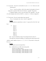
1
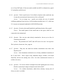
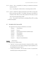
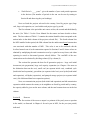
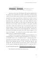
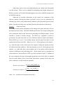
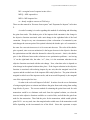
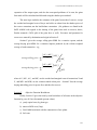
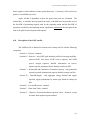
Long Term Model USER MANUAL, February 2001 expansion of the output report, and also has conceptual problems of its own, the gains from trade will be calculated and allocated using the shadow price method. The same logic underlies the estimates of the gains from trade of reserves, except the avoided and marginal costs of buyer and seller are taken from the shadow prices of the reserve constraints, not the load balance constraints. (No guidance was found in the SAPP ABOM with regards to the sharing of the gains from trade in reserves; hence, Purdue assumed a 50/50 split of the gains here as well.) Revenues and payments for reserves are entered by destination and origin in Section F. Section F gives the average selling price/MWh for a counties exports, and the average buying price/MWh for a countries imports produced by the volume-weighted average of each transaction – e.g., average selling price = ∑ AC x + MCx ( MWx ) 2 ∑ MW x x x average buying price = ∑ AC y + MC y ( MWy ) 2 y ∑ MW y y where ACx, MCx, ACy, and MCy are the avoided and marginal costs of transactions X and Y, and MWx and MWy are the volumes traded at that price. Section F lists the average buying and selling price for power first, and then for reserves. Section G Objective Function Breakdown Finally, Section G gives the term by term breakdown of all terms in the objective function by year; all $ are discounted (present values) a) yearly capital costs, by plant type b) unserved MW cost (if any) c) fixed O&M associated with the construction of new plants d) fuel costs 141