Download Stream Depletion Factor Model SDF View

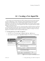
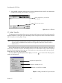
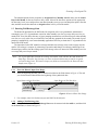
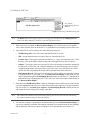
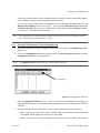
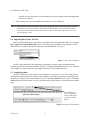
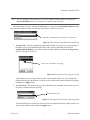
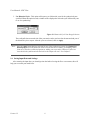
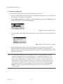
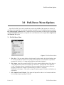
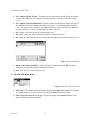
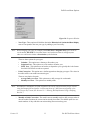
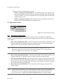
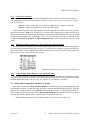
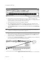
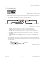
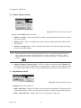
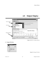
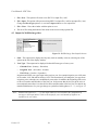
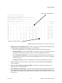
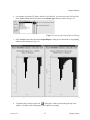
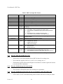
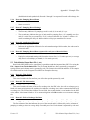
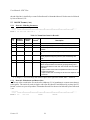
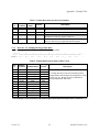
Stream Depletion Factor
Model
SDF View
User Manual - Version 1.2
Developed for the South Platte Advisory Committee by the Integrated
Decision Support Group (IDS) at Colorado State University
User Manual - SDF View
Stream Depletion Factor (SDF) View - Version 1.2
Copyright
Copyright © 1999 Integrated Decision Support Group
About This Document
This user manual describes the Stream Depletion Factor (SDF) View. The information presented here
parallels the on-line documentation available with the SDF View software and describes a program
developed to calculate stream accretions and depletions based on recharge and consumptive use data.
Participation
This project was created in order to meet the needs of as many water users in the South Platte as
possible. In order to develop a consensus on the data and modeling needs of the water users in the South
Platte Basin an advisory committee was formed. The committee is comprised of representatives from: the
Northern Colorado Water Conservancy District (NCWCD), the South Platte Lower River Group, Inc.
(SPLRG), the Colorado State Engineers Office (SEO), Goundwater Appropriators of the South Platte
(GASP), the Central Colorado Water Conservancy District (CCWCD), Lower South Platte Water
Conservancy District (LSPWCD), Colorado Water Resources Research Institute (CWRRI), City of
Greeley (Greeley), and the City of Fort Collins (Fort Collins). SDF View described in this manual is part
of the South Platte water management research being worked on by the Integrated Decision Support (IDS)
Group (a research group at Colorado State University).
For information about IDS contact:
For information about SDFView contact:
Luis Garcia -- IDS Group
601 South Howes, USC Suite 502
Colorado State University
Fort Collins, Colorado 80523 USA
Phone:
(970) 491-5144
Fax:
(970) 491-2293
E-mail:
garcia@ engr.colostate.edu
Jon Altenhofen - NCWCD
Northern Colorado Water Conservancy District
Post Office Box 679
Loveland, CO 80539
Phone:
(970) 667-2437
Fax:
(970) 669-1143
E-mail:
[email protected]
About the SDV View Software
The SDF Model computational program is written in standard FORTRAN. The SDF View model
interface is written in the C++ programming language and was constructed with visual C++. The
development and user platform is a PC running Windows 95/98/NT. The interface contains online help
parallel to this documentation and also contains a graphing package.
Installing the Software
1. Copy the sdfview.zip file into a directory on your machine where the winzip program is installed.
2. Using Microsoft Explorer double click on the sdfview.zip file. Winzip will open the file.
3. When the files appear in the browser window select the Install button in Winzip, the setup routine
will begin. (For more information see the http://www.ids.colostate.edu/projects/sdfview/)
4. Follow the instructions provided in the setup routine.
Version 1.2
ii
Table of Contents
Table of Contents
1.0 Creating a New Input File - - - - - - - - - - - - - - - - - - - - - - - - - - - - - - - - - - - - - - - - - - - - - - -1
1.1 Creating and Saving a New SDF View Input File - - - - - - - - - - - - - - - - - - - - - - - - - - - - -1
1.2 Setting Properties - - - - - - - - - - - - - - - - - - - - - - - - - - - - - - - - - - - - - - - - - - - - - - - - - - -2
1.3 Entering Well/Recharge Data - - - - - - - - - - - - - - - - - - - - - - - - - - - - - - - - - - - - - - - - - - -3
Enter the Historic Input Year Range - - - - - - - - - - - - - - - - - - - - - - - - - - - - - - - - - - - - - -3
Adding a Well/Recharge Site - - - - - - - - - - - - - - - - - - - - - - - - - - - - - - - - - - - - - - - - - - -3
Entering Well Information Using a Pumping Record - - - - - - - - - - - - - - - - - - - - - - - - - - -5
1.4 Importing Data from a Text File - - - - - - - - - - - - - - - - - - - - - - - - - - - - - - - - - - - - - - - - -6
1.5 Synthesizing Data - - - - - - - - - - - - - - - - - - - - - - - - - - - - - - - - - - - - - - - - - - - - - - - - - -6
1.6 Saving Input Data and Settings - - - - - - - - - - - - - - - - - - - - - - - - - - - - - - - - - - - - - - - - - -8
2.0 Running the SDF View Model - - - - - - - - - - - - - - - - - - - - - - - - - - - - - - - - - - - - - - - - - - - -9
2.1 Setting the Run Year Range - - - - - - - - - - - - - - - - - - - - - - - - - - - - - - - - - - - - - - - - - - - -9
2.2 Selecting the Output Type - - - - - - - - - - - - - - - - - - - - - - - - - - - - - - - - - - - - - - - - - - - - -9
2.3 Running an Input File - - - - - - - - - - - - - - - - - - - - - - - - - - - - - - - - - - - - - - - - - - - - - - - 10
3.0 Pull-Down Menu Options - - - - - - - - - - - - - - - - - - - - - - - - - - - - - - - - - - - - - - - - - - - - - - 11
3.1 File Pull-Down Menu - - - - - - - - - - - - - - - - - - - - - - - - - - - - - - - - - - - - - - - - - - - - - - - 11
3.2 The SDF Pull-Down Menu - - - - - - - - - - - - - - - - - - - - - - - - - - - - - - - - - - - - - - - - - - - 12
3.3 Edit Pull-Down Menu - - - - - - - - - - - - - - - - - - - - - - - - - - - - - - - - - - - - - - - - - - - - - - - 14
Edit Pull-Down Menu Options - - - - - - - - - - - - - - - - - - - - - - - - - - - - - - - - - - - - - - - - - 14
Control Key Functions - - - - - - - - - - - - - - - - - - - - - - - - - - - - - - - - - - - - - - - - - - - - - - 15
Right Mouse Button Options for Cutting and Pasting Individual Items - - - - - - - - - - - - - - 15
Using the Right Mouse Button to Copy and Paste Tables - - - - - - - - - - - - - - - - - - - - - - - 15
3.4 Cutting and Pasting Data from Other Programs - - - - - - - - - - - - - - - - - - - - - - - - - - - - - - 15
3.5 View Pull-Down Menu - - - - - - - - - - - - - - - - - - - - - - - - - - - - - - - - - - - - - - - - - - - - - - 17
3.6 Window Pull-Down Menu - - - - - - - - - - - - - - - - - - - - - - - - - - - - - - - - - - - - - - - - - - - - 18
3.7 Help Pull-Down Menu - - - - - - - - - - - - - - - - - - - - - - - - - - - - - - - - - - - - - - - - - - - - - - 18
4.0 Output Display - - - - - - - - - - - - - - - - - - - - - - - - - - - - - - - - - - - - - - - - - - - - - - - - - - - - - 19
4.1 Output File Menu - - - - - - - - - - - - - - - - - - - - - - - - - - - - - - - - - - - - - - - - - - - - - - - - - - 19
4.2 Output for Well/Recharge Sites - - - - - - - - - - - - - - - - - - - - - - - - - - - - - - - - - - - - - - - - 20
4.3 Output Buttons - - - - - - - - - - - - - - - - - - - - - - - - - - - - - - - - - - - - - - - - - - - - - - - - - - - 22
iii
User Manual - South Platte SDF View
4.4 Plotting Output - - - - - - - - - - - - - - - - - - - - - - - - - - - - - - - - - - - - - - - - - - - - - - - - - - - 22
5.0 Appendix I: Example Files - - - - - - - - - - - - - - - - - - - - - - - - - - - - - - - - - - - - - - - - - - - - - 25
5.1 Example SDF View Input File (*.sdf) - - - - - - - - - - - - - - - - - - - - - - - - - - - - - - - - - - - - 25
Record 1: Version Number - - - - - - - - - - - - - - - - - - - - - - - - - - - - - - - - - - - - - - - - - - - - 25
Record 2: Modeling Parameters - - - - - - - - - - - - - - - - - - - - - - - - - - - - - - - - - - - - - - - - 25
Record 3: SDF and Well/Recharge Site - - - - - - - - - - - - - - - - - - - - - - - - - - - - - - - - - - - 26
Record 4: Well/Recharge Site Name and ID - - - - - - - - - - - - - - - - - - - - - - - - - - - - - - - - 26
Record 5: Well/Recharge Data (Records 3-5 are repeated for each well/recharge site) - - - 26
Record 6: Pumping Record Name - - - - - - - - - - - - - - - - - - - - - - - - - - - - - - - - - - - - - - - 27
Record 7: Pumping Record Settings - - - - - - - - - - - - - - - - - - - - - - - - - - - - - - - - - - - - - - 27
Record 8: Application Efficiencies - - - - - - - - - - - - - - - - - - - - - - - - - - - - - - - - - - - - - - - 27
Record 9: Pumping Record Data (repeated for each year of historical data) - - - - - - - - - - 27
5.2 Tab-delimited Input Data File (*.txt) - - - - - - - - - - - - - - - - - - - - - - - - - - - - - - - - - - - - - 27
Record 1: Time Period - - - - - - - - - - - - - - - - - - - - - - - - - - - - - - - - - - - - - - - - - - - - - - 27
Record 2: File Information - - - - - - - - - - - - - - - - - - - - - - - - - - - - - - - - - - - - - - - - - - - - 27
Record 3: Well or Recharge Site Data - - - - - - - - - - - - - - - - - - - - - - - - - - - - - - - - - - - - 27
5.3 Old SDF Format (*.txt) - - - - - - - - - - - - - - - - - - - - - - - - - - - - - - - - - - - - - - - - - - - - - - 28
Record 1: Modeling Parameters - - - - - - - - - - - - - - - - - - - - - - - - - - - - - - - - - - - - - - - - 28
Record 2: Withdrawal and Return Sites - - - - - - - - - - - - - - - - - - - - - - - - - - - - - - - - - - - 28
Record 3: CU Pumping/Recharge Input Rates - - - - - - - - - - - - - - - - - - - - - - - - - - - - - - - 29
6.0 Index - - - - - - - - - - - - - - - - - - - - - - - - - - - - - - - - - - - - - - - - - - - - - - - - - - - - - - - - - - - - - 31
Version 1.2
iv
Creating a New Input File
1.0 Creating a New Input File
Water managers use Stream Depletion Factors (SDF) to determine the lag time from when irrigation
well water is pumped from, or water is recharged to, an alluvial unconfined river aquifer and when a
depletion or accretion happens in the river. Required input information for SDF View is irrigated
consumptive use from well water or net recharge amounts and SDF values for irrigation wells or recharge
basins. This section describes how to create an input file for the SDF View program, which then computes
depletions or accretions to the river.
SDF input files can be created as a new file, created in the pending CU Model and imported, or imported
from a previous SDF input format. This section will describe the steps needed to create a new SDF View
input file. Another approach to making an SDF View input file is to modify an existing file. All of these
approaches are described in “Section 3.0: Pull-Down Menu Options”.
1.1 Creating and Saving a New SDF View Input File
1. Open SDF View by selecting the Start > Programs > SDF View > SDF View icon.
2. Select the File > New option and the Input Editor Window will be displayed with blank fields.
Well/Recharge Site Information
Input Historical Years
Historical Data Display
Synthesized Data Display
Figure 1: New File Option with Blank Input Window
Version 1.2
1
Creating and Saving a New SDF View Input File
User Manual - SDF View
3. Select the File > Save As option and select a location and name for the input file, the default name
is SDFVie#.sdf starting with 1 for the #, see Figure 2.
Select the directory you want to
save the file
Enter in a new name
Figure 2: Save As Window
1.2 Setting Properties
The properties pop-up window allows you to enter data in the format you want. Data can be entered in
irrigation, calendar, or USGS year types with monthly totals or average daily values, but the model will run
only in irrigation year using daily averages.
Note - Enter new data as monthly totals and allow the model to do the conversion to daily values,
since the factor or method used to compute the average daily values may not be the same as
what you used.
Most of the time data are available in monthly totals, therefore the conversion used to run the model in
average daily values has two options. The default option is to use actual numbers of days in the month with
this conversion taking into account leap years. You can also use a conversion rate that is the same for all
months and years (30.417 days per month).
Select the SDF > Properties (Units & Year Type), or select the
icon in the toolbar. The properties
window will be displayed.
Default is Irrigation Year
Default is Monthly Acre-Ft
Default is Actual Days in Month
Figure 3: Setting Unit and Year Type Properties
Version 1.2
2
Creating a New Input File
The standard options for the properties are Irrigation Year, Monthly Acre-Ft and to use the Actual
Days in the Month for the conversion to daily values. Most of the time these options will be appropriate
for data entry, but if you would prefer to enter data in another year type you can change the option, enter the
data, and then convert the data back to Irrigation Year before you run the model.
1.3 Entering Well/Recharge Data
The historical input data for the SDF model for irrigation wells is net groundwater withdrawal or
consumptive use (CU) of groundwater entered as either monthly acre-feet or average daily acre-feet per
month. SDF View also allows the entry of gross pumping amounts from well flow meters as either monthly
acre-feet or as a cfs (cubic feet per second) flow rate and days pumped for the month. The record of gross
pumping is multiplied by a user entered monthly application efficiency to obtain the CU of groundwater for
input to the SDF model.
The input data for the SDF model for recharge should be net recharge values or the seepage into the
aquifer. Net recharge is compute by subtracting evaporation and changes in recharge pond storage from
measured gross inflows into the recharge pond. Net recharge values are entered as either monthly acre-feet
or average daily acre-feet per month.
Note - For a given SDF Run Scenario all recharge sites and/or wells will have the same historical
data range. Therefore, the first step is to select an historical data time period for irrigation
well and recharge sites. The historical input year fields are located above the historical data
display area (Figure 4).
1.3.1
Enter the Historic Input Year Range
1. Enter the beginning and end years of the historical data in the fields shown in Figure 4. The end
year for the historical data defines the beginning of the synthesized data.
Input Historical Start Year Here.
Input Historical End Year Here
Figure 4: Historical Data Year Range
2. For example, enter 1991 for the start year and 1992 for the end year.
1.3.2 Adding a Well/Recharge Site
To add a specified amount of Well/Recharge Sites enter the amount in the # to add box, and then click
on the New button, as shown in Figure 5.
Version 1.2
3
Entering Well/Recharge Data
User Manual - SDF View
}
Site Description List
New, Delete
and Pumping Record
Buttons.
Figure 5: Selecting a Well/Recharge Site
Note - The Delete button will bring up a menu for selecting sites to be deleted. The Pumping Record
button will add a pumping record for a selected Irrigation well site.
3. When a new site(s) is added, the Historical Data Display area is filled with zeros for monthly
values. Enter in actual values for historical CU of groundwater or net recharge in place of the zeros.
4. Type in data for the well or recharge site in the following categories:
•
Well/Recharge Sites - This is the name and identification for the site.
•
SDF - Stream depletion factors in units of days are entered in this field.
•
Location Type - This toggle switch with two choices, i.e., “Irrig. well or Recharge site”. Click
the entry you want to change with the mouse and it will toggle between the two choices.
•
Output? - This toggle switch is used to specify if the well/recharge site should be included in
the output file. If you select “no,” then the computation for the well/recharge site will not be
computed and no output will be generated. If you select “yes,” the well/recharge site will be
used for the SDF computation and output will be generated when the model is run.
•
Has Pumping Record - This toggle switch controls if a well record for gross pumping was used
to compute well CU. If you select “yes”, then Historical Data Display for the given well can
only be changed through the Well Pumping Record window (See Section 1.3.3 “Entering Well
Information Using a Pumping Record”). If you select “no” then values can be edited directly in
the Historical Data Display.
5. Enter data in the Well/Recharge Sites window by clicking the mouse with the cursor in the cell (the
cell will be highlighted and a text cursor will be placed to the right of the text). For options that have
only two choices (i.e. Location Type, Output?, and Has Pumping Record), clicking on the cell
will change the current setting (for example, yes to no).
Note - The width of the columns can be increased by placing the cursor on the title bar and moving
the column separator along the top of the display.
6. You can enter recharge or consumptive use amounts directly into the Historical Data Display, or
you can use pumping records that will compute consumptive use amounts based on gross pumping
and an application efficiency to obtain consumptive use of groundwater (See Section 1.3.3
Version 1.2
4
Creating a New Input File
“Entering Well Information Using a Pumping Record”). Pumping records contain daily pumping
rates or monthly pumping volumes and application efficiencies.
7. For each site, enter the historical CU of groundwater or net recharge data by month and year in the
Historical Data Display area shown in Figure 1, for the period of Historical Start Year through
the Historical End Year. The unit type and year type can be edited using the Properties window,
see “Section 3.2: The SDF Pull-Down Menu”.
Note - The heading above the Historical Data Display lists the name of the well/recharge site and
the current settings for the unit and year types.
1.3.3
Entering Well Information Using a Pumping Record
1. Select the irrigation well site by clicking the mouse on the site name in the Well/Recharge Sites
display area.
2. Click on the Pumping Record button on the right side of the Well/Recharge Sites display, and the
Pumping Record window will be displayed.
Note - The Pumping Record button is only active for irrigation well sites.
Units Setting
Figure 6: Pumping Record Window
3. Enter the Application Efficiency (0.0 - 1.0), this is a factor that is multiplied by the monthly gross
pumping to get consumptive use amounts from the pumping records. For example enter 0.5 for 50%
efficiency.
4. Select the discharge measurement units for gross pumping amounts, there are two choices:
•
CFS - Cubic feet per second, enter values for the discharge rate, the number of days of operation
each month, and the application efficiency for each month.
•
Ac-Ft - Acre feet, one foot of water distributed uniformly over one acre of land. Enter monthly
Version 1.2
5
Entering Well/Recharge Data
User Manual - SDF View
values for acre feet. Since this is a volume and not a rate, only a monthly total and an application
efficiency are entered.
5. After entering your values select OK and a warning box will be displayed.
Note - Selecting OK in the warning box will enter the computed well CU from the pumping record
and replace any previous values in the Historical Data Display area. If you do not want to
replace previously inputted values, then first save them as a new file name before you enter
a new pumping record.
1.4 Importing Data from a Text File
Data for the SDF Model can be entered into a spreadsheet and then imported into SDF View using the
File > Import from Tab-delimited File option. To use this option, spreadsheet files should be saved in
Microsoft Excel or another spreadsheet program as a tab-delimited file, see Figure 7.
Figure 7: Excel Save As Options
The file format should have lines separated by paragraph or carriage returns and column entries
separated by tabs. The format is described in “Section 5.2: Tab-delimited Input Data File (*.txt)” and there
is an example file called testsdf.txt in the \Program Files\SDFView\Examples directory.
1.5 Synthesizing Data
The SDF model can be used to project future depletions or accretions to a river. This is done first by
entering known historical data for recharge and consumptive use and then projecting or synthesizing into
the future. To synthesize data, enter the number of years in the Years of Data field, see Figure 8. The Years
of Data field specifies the number of years to synthesize data, starting from the year after the historical data
range.
Enter Number of
Years to Synthesize
Here and Hit Enter
or the Recalculate
Button.
Synthesized Data Display
Figure 8: Synthesize Data Window
Version 1.2
6
Creating a New Input File
Note - For an existing file input window, if new sites are added or historical data is changed, the
Recalculate Button must be clicked in order to update synthesized data.
After the number of years is selected and the Enter key is pressed or the Recalculate Button clicked,
the type of data synthesis can be selected from three choices, as shown in Figure 9.
Methods are displayed by selecting the scroll arrow.
Figure 9: Choose Synthesizing Method Pop-up Window
1. Average Years - This data synthesizing option will calculate an average over a selected range of
historical years for each month and paste these values for the synthesized period into the
Synthesized Data Display area. A data selection window is displayed when the Average Years
option is selected, see Figure 10.
Years to be selected for averaging.
Figure 10: Selecting Years for Using the Average
Select multiple years to average using the shift, control, and/or arrow keys, or by clicking and
pulling down the list with the mouse. Once the years are selected the synthesized data is created by
clicking on the Apply button.
2. Use Given Year - This option will copy a given historical year’s monthly values to each year over
the range of synthesized years specified.
Selected Given Year
Figure 11: Selecting a Given Year for Synthesizing Data
Select the historical year of data you want to use for the synthesized period by clicking on the year
in the pop-up window, and selecting the Apply button.
Version 1.2
7
Synthesizing Data
User Manual - SDF View
3. Use Historical Cycle - This option will repeat a set of historical years for the synthesized years
specified. When this option is used, a window will be displayed to select the cycle of historical years
to use for synthesizing.
Figure 12: Historical Cycle Year Range Selection
The scroll pull-downs on each side of the year entries can be used to select the start and end year of
the historical cycle to repeat. After the years are selected, click on Apply.
Note - Once the Apply button has been selected for any of the synthesizing options, the Synthesized
Data Display area will be filled with values. You can also enter in values, by modifying values
from one of the other synthesized options or adding your own values. When new values are
entered into the synthesized table the label in the output will read “User Defined”.
1.6 Saving Input Data and Settings
After entering the input data, you should get into the habit of saving the file to a new name, this will
help you to recreate past model runs.
Version 1.2
8
Running the SDF View Model
2.0 Running the SDF View Model
2.1 Setting the Run Year Range
Set the Run Year Range at the bottom of the Input Editor window, see Figure 1 and Figure 13. If the
run range is greater than the historical range and the synthesized range, zero values for recharge and/or
consumptive use values will be used for the entries after the historical and synthesized ranges.
Figure 13: Run Year Range
For example, if there are two years of historical data (1991-1992) and there are two years of synthesized
data (1993-1994), the run years will be (1991-1994) by default. But if you enter (1991-1996) for the run
years (Figure 13), the years (1995-1996) will be run in the SDF Model with zero values for recharge or
consumptive use.
2.2 Selecting the Output Type
The type of output that will be produced when the model is run can be set in the Input Editor window
next to the run years, see Figure 13. There are two options for output display as shown in Figure 14.
Figure 14: Selecting Output Type
•
by well/recharge site - This option creates output for each well/recharge site as well as totals
and averages for all the sites.
•
only totals for all well/recharge sites - This option only creates output for the totals for all the
sites and does not include information by individual site.
Note - In the output, a recharge site is summed as a positive value (accretion) and a well is summed
as a negative value (depletion).
Version 1.2
9
Setting the Run Year Range
User Manual - SDF View
2.3 Running an Input File
To run an SDF input file follow these steps after an input file is created:
1. Open an existing SDF Input File (See Section 3.1 “File Pull-Down Menu”) or create a new SDF file
(See Section 1.0 “Creating a New Input File”).
2. select the SDF > Run option (See Section 3.2 “The SDF Pull-Down Menu”) or the Run icon in the
toolbar (See Section 3.5 “View Pull-Down Menu”).
Figure 15: Selecting the Run Option
3. A pop-up window will be displayed with the option to save the input file if it has not already been
saved.
Figure 16: Input File Save Pop-Up Window
4. Select the Yes button, the input file will be saved and run. The output for the model will be
displayed in the main window using the output display (See Section 4.0 “Output Display”). The
output file will have the same name as the input file, but with a *.out extension instead of the *.sdf
extension of the input file.
Note - The SDF Model can only run in the Irrigation year (Nov. - Oct.) format and a warning is
displayed to change to this year type (See Section 3.2 “The SDF Pull-Down Menu”). In
converting to irrigation year to run the SDF Model, zero values are entered as historical
values for any added months. For example, if historical data is entered in calendar year
format (Jan-Dec) and then changed to irrigation year, another year is added at the end of the
historical data to include the Nov. and Dec. data with zero values for Jan. through Oct. of
this added irrigation year. When changing year type in order to run the SDF model, BE
SURE to check that synthesized data is still appropriate, otherwise recalculate the
synthesized data.
Version 1.2
10
Pull-Down Menu Options
3.0 Pull-Down Menu Options
Input files for SDF View can be created from scratch using the File > New option (See Section 1.0
“Creating a New Input File”), created in the pending Consumptive Use (CU) Model and opened with the
File > Import from CU Model option, or imported from a previous format of SDF input files using the File
> Import Old SDF Format option, or imported from a tab-delimited text file using the File > Import from
Tab-delimited File option.
3.1 File Pull-Down Menu
Figure 17: File Pull-Down Menu
1. File > New - The new option displays a blank input file editor window in which all the data must
be entered by hand (See Section 1.0 “Creating a New Input File”) or pasted from a spreadsheet
program (See Section 3.4 “Cutting and Pasting Data from Other Programs”).
2. File > Open - Input files created with SDF View can be opened with this option, if they have an
*.sdf extension and are in the correct format (See Section 5.1 “Example SDF View Input File
(*.sdf)”). When the software is installed it will create example files in the directory where the
program is installed, for example it will most likely be saved in ‘C:\Program
Files\SDFView\Examples’. There will be an input file and an output file called test.sdf and test.out,
respectively.
3. File > Import From CU Model - This option will import files with an *.owl extension that have
been creating using the pending CU Model.
Version 1.2
11
File Pull-Down Menu
User Manual - SDF View
4. File > Import Old SDF Format - This option can be used to import an SDF file for the original
version of the SDF Model. An example file format is shown in “Section 5.3: Old SDF Format
(*.txt)”.
5. File > Import from Tab-delimited File - Imports a dataset into the Historical data field. The text
file should be in the correct format as described in “Section 5.2: Tab-delimited Input Data File
(*.txt)”. The dataset can be created in a spreadsheet and saved as a text file that can be imported
using this option, see “Section 1.4: Importing Data from a Text File”.
6. File > Close - Closes the current file with an option to save.
7. File > Save - Saves the current version of the input file with the same name.
8. File > Save As - This option allows you to change the name and location of the file when you save it.
Figure 18: Save As Window
9. Display of Recently Opened Files - The files in the list on the bottom of the File pull-down
window can be opened by clicking on them with the mouse.
10. Exit - Exits SDF View with an option to save.
3.2 The SDF Pull-Down Menu
Figure 19: The SDF Pull-Down Menu
1. SDF > Run - This option runs the SDF Model and opens the Output View Window (See Section
4.0 “Output Display”). This is the same as clicking on the Run Button in the toolbar.
2. SDF > Properties (Units & Year Type) - This option displays the Properties Window, with
options for unit conversion and display.
Version 1.2
12
Pull-Down Menu Options
Figure 20: Properties Window
•
Year Type - These options will shift the data in the Historical and Synthesized Data Display
areas to correspond to the new year type, by adding a year if necessary.
Note - When changing year types, for example from USGS Year to Irrigation Year type in order to
run the model, BE SURE to check that historic and synthesized data is still appropriate
otherwise edit historical data or Recalculate synthesized data.
•
There are three options for year types:
• Calendar - This option uses a January to December year.
• Irrigation Year - This option uses a November to October year.
• USGS Year - This option uses an October to September year, typically this is the format
for which USGS flow records are reported.
Units Conversion - This option uses a similar approach as changing year types. The values in
the tables will be converted between unit types.
There are two choices for units:
• Average Daily Acre Feet - This option uses a daily average for each month.
• Monthly Acre Feet - This option uses monthly totals.
Note - Groundwater consumptive use from irrigation wells can be entered in cubic feet per second
using the Pumping Record option, A conversion factor of 1.9835 from average daily cfs to
acre-feet per day is used. (See Section 1.3.3 “Entering Well Information Using a Pumping
Record”).
•
Version 1.2
Monthly to Daily Conversion - The model converts monthly totals to daily averages when it
does the model run unless the conversion has already been done. The default option is to use
actual numbers of days with this conversion taking into account leap years.
13
The SDF Pull-Down Menu
User Manual - SDF View
There are two options for doing this conversion:
• Will Use Average Days in Month (30.417) - This selection will use an average of 30.417
days per month to make the conversion between monthly and daily values when the model
is run. For example, a conversion of monthly totals to average daily values will divide the
monthly totals by 30.417.
• Will Use Actual Days in Month - This selection will use actual numbers of days in the
month with this conversion taking into account leap years.
3.3 Edit Pull-Down Menu
Figure 21: The Edit Pull-Down Menu
3.3.1 Edit Pull-Down Menu Options
The copy and paste function use the Windows 95/98/NT concept of a clipboard. A clipboard is a
temporary location in the computer’s memory where information is stored before it is pasted or another item
is cut or copied.
1. Edit > Copy from Historical Table - Copies the contents of the entire historical input table to the
computers clipboard. The clipboard contents are separated by tabs for columns and paragraph
returns for rows. This data can then be pasted into other programs.
Note - There is no way to directly view the contents of the computer’s clipboard. To see the
information saved there you must paste it into another program (i.e. by selecting the paste
option in the Edit pull-down menu of the other program).
2. Edit > Copy from Synthesized Table - Copies the entire contents of the synthesized table to the
computers clipboard. The clipboard contents can then be pasted into another program.
3. Edit > Paste into Historical Table - Pastes the contents of the computers clipboard to the historical
table. The contents of the clipboard should be a table with 13 columns (the first column is the years,
and the other 12 columns are monthly data). The number of rows should correspond to the number
of years specified for the appropriate table.
4. Edit > Paste into Synthesized Table - Pastes the contents of the computers clipboard to the
synthesized table.
Note - Clipboard contents must have entries separated by tabs with the end of the line signified by
a paragraph return. The clipboard contents must have the same number of columns as the
table being pasted into. Entries CAN NOT be left blank, enter a zero “0” for no value.
Version 1.2
14
Pull-Down Menu Options
3.3.2 Control Key Functions
These functions can also be activated by holding the keyboard control key down and pressing the
corresponding letter for the following control key option, with the cursor in the window you are copying
from or pasting to:
• control-c - Copies all the items in the selected window into the computer’s clipboard.
•
control-v - Pastes the clipboard items to the specified window.
These functions typically work in all Windows 95/98/NT programs even if there is not a copy or paste
option in the program’s Edit menu. The SDF View version of these functions copies and pastes the entire
table in the selected data display window. Remember if pasting into the Well/Recharge Site area of the input
window, the clipboard must have 5 non-blank (i.e. use “x”s) columns separated by tabs, even though the last
3 columns (Location Type, Output?, and Has Pumping Record) will not be pasted because they are fixed
values.
3.3.3 Right Mouse Button Options for Cutting and Pasting Individual Items
Press the right mouse button in any of the data windows and a small menu will be displayed with options
for cutting and pasting individual items, see Figure 22. To display these options, you must click the right
mouse button when a cell is highlighted for editing with the cursor over the selected cell. This option can
only be used to copy, cut or paste one item at a time.
Figure 22: Right Mouse Options for Cutting and Pasting
3.3.4 Using the Right Mouse Button to Copy and Paste Tables
If you click the right mouse button in a data display area outside of the data cells, the right mouse menu
will give you the option to copy or paste. This option works the same as the control key options for, selecting
the entire data display table to copy or paste, see “Section 3.3.2: Control Key Functions”.
3.4 Cutting and Pasting Data from Other Programs
Data can be entered into the Historical Data Display or other data windows by cutting and pasting from
a spreadsheet, text editor, or word-processing program by using the standard Windows 95/98/NT keyboard
functions or by using the options in the Edit pull-down menu (See Section 3.3 “Edit Pull-Down Menu”).
This example will show how to paste into the Historical Data Display using the Microsoft Excel program,
but other spreadsheet programs such as Quatro Pro can be used in the same way.
1. In the spreadsheet program Excel, display the data you want to copy into SDF View.
Version 1.2
15
Cutting and Pasting Data from Other Programs
User Manual - SDF View
Figure 23: Selected Data in Excel
2. Select the data you want to paste into SDF View as in Figure 23 and press control-c on the
keyboard. You must select the year column and twelve months of data (i.e. 13 columns of data). All
the cells should have an entry since blank cells will create errors.
3. The data selected will be copied to your computer’s clipboard.
4. Enter an Historical Start and End Year corresponding to the data on the clipboard, for this
example the Historical Start Year is 1991 and the Historical End Year is 1992, see Figure 23.
5. Add a Well\Recharge Site(s) by pressing the New button on the right side of the Well\Recharge
Site display.
Note - If you want to add historical years to correspond to the data being pasted, enter them in the
historical year cells before you paste the data, see Figure 24.
6. Make sure the water year type and the units selected for the historical data correspond to the data
being pasted. These settings can be changed using the Properties option in the SDF pull-down
menu (See Section 3.2 “The SDF Pull-Down Menu”).
7. Click the mouse in the Historical Data Display area, and press control-v, see Figure 24. Make sure
the years being copied are the same as the historical year period.
Input Data
should match
years being
pasted.
Historical Data Display
Figure 24: SDF Data Paste for Consumptive Use of Groundwater.
Version 1.2
16
Pull-Down Menu Options
3.5 View Pull-Down Menu
Figure 25: The View Pull-Down Menu
The View pull-down menu has two options, that are toggle switches to change the SDF View display:
1. View > Toolbar - This displays the tool bar with the following options:
New File
Open File
Save File
Run Model Open Properties
Figure 26: SDF View Toolbar
•
New File - Opens new input file, see “Section 1.0: Creating a New Input File”.
•
Open File - Opens existing input file, see “Section 3.1: File Pull-Down Menu”.
•
Save File - Saves current version of input file, see “Section 3.1: File Pull-Down Menu”.
•
Run Model - Runs the SDF Model with current input file, see “Section 3.2: The SDF PullDown Menu”.
•
Open Properties - Opens the Properties window, see “Section 3.2: The SDF Pull-Down
Menu”
2. View > Status Bar - The status bar contains information about the workings of the program and
can be displayed or not depending on the setting of the option. It is located in the lower left corner
of the main window.
Status Bar
Figure 27: Status Bar
Version 1.2
17
View Pull-Down Menu
User Manual - SDF View
3.6 Window Pull-Down Menu
Figure 28: The Window Pull-Down Menu
Options for the Window pull-down menu:
3. Window > Cascade - If there are multiple file windows open, this option will cascade the windows
in the main window.
4. Window > Tile - If there are multiple file windows open, this option will tile the windows in the
main window.
5. Window > Arrange Icons - If there are multiple file windows iconified, this option will arrange
the icons in the main window.
Note - Input file windows can be iconified, displayed in full-view, or closed using the buttons on the
upper right of each window. The horizontal line iconifies a window, the square or double
square displays the window in full or partial view, respectively and the “x” symbol closes the
window.
6. Display of Windows Currently Open - The list of windows on the bottom of the Window pulldown menu displays all the windows that are currently opened, a window can be brought to the front
by clicking on the window in the list. The currently displayed window has a check mark next to it.
3.7 Help Pull-Down Menu
Figure 29: The Help Pull-Down Menu
The Help pull-down menu option are:
1. Help > Help Topics - Displays the online version of the help documentation. This online help file
parallels this document. There is an index and search features available with the online help files.
2. Help > About SDF View - Displays the current version number of SDF View.
Version 1.2
18
Output Display
4.0 Output Display
Scale of Data
Year Type
Output Data Display
Output Buttons
Figure 30: SDF View Output Window
4.1 Output File Menu
Figure 31: Output File Menu
Version 1.2
19
Output File Menu
User Manual - SDF View
1. File > New - This option will create a new SDF View input file (*.sdf).
2. File > Open - This option will open an existing SDF View input file (*.sdf) or an output file (*.out).
Change the files of type option to (*.out) in the Open window to view output files.
3. File > Close - Closes the window with the option to save.
4. The list of files along the bottom of the menu are the most recently opened files.
4.2 Output for Well/Recharge Sites
Figure 32: Well/Recharge Site Output Selection
1. Scale - The output can be displayed with yearly totals or monthly values by selecting one of the
options to the left of the display window.
2. Year Type - The output can be displayed in three different types of water years.
•
Calendar Year - (January - December)
•
Irrigation Year - (November - October)
•
USGS Year - (October - September)
Irrigation and USGS year types begin in the previous year, for example irrigation year 1992 starts
in November, 1991 and ends in October, 1992. This means that if you change the year type from
irrigation year to calendar year, an additional year needs to be added to the beginning of the series
to show November and December of the first year. It also means that the last year in the series is
not complete because there is no data for November and December of the last year. The data for any
months added because of a year type change are symbolized with hyphens (i.e. “-”), see Figure 33.
Note - Months with hyphens (i.e. “-”) in the output tables are not included in the computation of
averages in the output tables. Totals in the output for years with months of hyphens are
assumed to be zero values.
Version 1.2
20
Output Display
Hyphens for Added Months.
The last year of historical data is 1997
There are 5 year(s) of synthesized data.
SYNTHESIZED DATA WAS GENERATED USING HISTORICAL DATA YEAR 1994
No well CU/Recharge after year 2002
Location: 646533 (farm 1)
CU or Recharge Data
YEAR
JAN
FEB
Location Type = Irrig. well
SDF = 80 days
( acre feet )
MAR
APR
MAY
JUN
JUL
AUG
SEP
OCT
NOV
DEC
TOTAL
CUMULATIVE
TOTAL
-------------------------------------------------------------------------------------------------------------1991
-
-
-
-
-
-
-
-
-
-
0
0
0
0
1992
0
0
0
0
0
-11.7
-47.1
-32.4
-3
0
0
0
-94.2
-94.2
1993
0
0
0
0
0
-6.5
-70.9
-38.1
-20.2
0
0
0
-135.7 -229.9
1994
0
0
0
-0.4
-10.2
-38
-58.7
-85.5
-27.3
0
0
0
-220.1 -450
1995
0
0
0
0
0
0
-24.3
-79.9
-35.6
-4.7
0
0
-144.5 -594.5
1996
0
0
0
0
0
-11.7
-47.1
-32.4
-3
0
0
0
-94.2
1997
0
0
0
0
-5.3
-4.8
-73.8
-59.6
-34.1
0
0
0
-177.6 -866.3
1998
0
0
0
-0.4
-10.2
-38
-58.7
-85.5
-27.3
0
0
0
-220.1 -1086.4
1999
0
0
0
-0.4
-10.2
-38
-58.7
-85.5
-27.3
0
0
0
-220.1 -1306.5
2000
0
0
0
-0.4
-10.2
-38
-58.7
-85.5
-27.3
0
0
0
-220.1 -1526.6
2001
0
0
0
-0.4
-10.2
-38
-58.7
-85.5
-27.3
0
0
0
-220.1 -1746.7
2002
0
0
0
-0.4
-10.2
-38
-58.7
-85.5
-27.3
0
-
-
-220.1 -1966.8
Avg
0
0
0
-0.22
-6
-24
-56
-69
-24
-0.43
0
0
-160
-688.7
-
Hyphens for Added Months.
Figure 33: Output Data Display with Change in Year Type
3. Output Type For Well/Recharge Sites - There are four types of output that can be displayed by
using the mouse to highlight the output type(s), as listed below:
•
Individual Well/Recharge Sites - Displays the data for individual well/recharge sites.
•
Recharge Summary - This contains monthly values and/or yearly totals for the amount of net
recharge and corresponding accretion to the river from all recharge sites summed.
•
CU of Groundwater Summary - This contains monthly values and/or yearly totals for the CU
of groundwater by irrigation wells and corresponding depletions to the river from all irrigation
well sites summed.
•
Net Impact on Stream - This is a summation of all accretions and depletions to the river.
4. Years - Displays yearly values and/or average values over the modeling period. Highlight the
year(s) to display
5. Show CU of Groundwater/Net Recharge Data - This option will display input data for net
recharge and/or CU of groundwater.
6. Show Depletion/Accretion Data - This option will display the depletion/accretion impacts at the
river computed by the SDF model. Depletions are the amount of water withdrawn from the river
due to the CU from irrigation wells and accretions are the amount of water returned to the river from
recharge sites.
Version 1.2
21
Output for Well/Recharge Sites
User Manual - SDF View
Note - CU of groundwater and depletions are shown in the output as negative values. Net recharge
and accretions are shown as positive values.
4.3 Output Buttons
Figure 34: Buttons for Saving, Printing and Plotting Output Data
1. Print - This button prints a text file with the output selected.
2. Save to File - This option can be used to save the contents of the output display to a text file. When
this option is selected, a window will be displayed to select a name and location for the file. The file
will be saved with returns separating rows and tabs separating column items.
Note - This file can then be imported into a spreadsheet program. By clicking on the right mouse
button in the output display area a copy/select menu will be displayed to copy items to the
clipboard.
3. Plot - This option can be used to plot the output specified, see “Section 4.4: Plotting Output”.
4. View in Wordpad - Allows the viewing of all the data in the Output Display area in Microsoft
Wordpad, so that the printing format (landscape/portrait) and the font can be customized.
5. Done - Closes this window and returns to the Input Editor window.
6. Help - Displays help on the output window parallel to this document.
4.4 Plotting Output
A graphing package has been incorporated into SDF View to display output. To view and print graphs
of output data follow these steps:
1. Arrange the data in the Output Display the way you want. You can select individual or multiple
sites and individual years or averages over the entire period. You can also select different year
types, or just show monthly or yearly totals.
Version 1.2
22
Output Display
2. For example, to plot 646533 (farm 1) data for 1992 and 1993, you can select years 1992 and 1993
in the Years column and the farm name in the Output Type column as shown in Figure 35.
Figure 35: Selecting the Output Data for Plotting
3. Select the Plot button when data in the Output Display is what your are interested in. The graphing
window will be displayed, Figure 36.
Figure 36: Plotting Windows for Diversion and Depletion Data (Summary data for farms in test.sdf file)
4. To print the plots select the print icon
in the plot’s window, located along the top of the
window. A window will be displayed to select options for printing.
Version 1.2
23
Plotting Output
User Manual - SDF View
5. The graphing package has numerous options to change the plots appearance which are obtained
through the tool bar at the top of the plots. The graphing package also has on-line help and can be
accessed by clicking on the help icon
Version 1.2
.
24
Appendix I: Example Files
5.0 Appendix I: Example Files
5.1 Example SDF View Input File (*.sdf)
This file is created by SDF View and is in a free format with the input information for SDF View.
5.1.1 Record 1: Version Number
This is the file version number, the version number is updated when changes are made to the input file
format. This section will describe version 1.2 of the input file.
Record 1:
Version 1.2
5.1.2 Record 2: Modeling Parameters
The first record includes the input, simulation, output, and projection start and end years, the number of
wells, the output format, the projection format, the type of year and units the data is saved in. The labels
correspond to the data in the entries.
Record 1:
1992 1997 5 1992 2002 4 0 2 2 0 1 1 0 # inputStartYear inputEndYear noOfSimulationYears
outputStartYear outputEndYear nwells outputFormat synthesizeFormat projYearStart
projYearEnd yearMode unitMode useAvgDaysPerMonth
Version 1.2
25
Example SDF View Input File (*.sdf)
User Manual - SDF View
Table 1: SDF View Input File Format
Variable Name
Format
Description
inputStartYear
Integer
Historical data beginning year.
inputEndYear
Integer
Historical data ending year.
noOfSimulationYears
Integer
The number of years to be synthesized.
outputStartYear
Integer
The output starting year.
outputEndYear
Integer
The output ending year.
nwells
Integer
The Number of wells/recharge sites in the input data.
outputFormat
Integer
(0 or1)
Indicates if the output will display information for each site (0) or totals for all
the sites (1).
synthesizeFormat
Integer
(1-4)
Indicates the type of projection used, the options are:
1 - Use Average - Uses an average of a period of years.
2 - Use Given Year - Repeats the given year over the synthesized
period.
3 - Use Historical Cycle - Repeats a series of years.
4 - User Defined - Used to indicate a user edited version.
projStartYear
Integer
Indicates year after input start year (=0) for the beginning year of the
projection method.
projEndYear
Integer
Indicates the end year of projection method.
yearMode
Integer
(0-2)
Defines the type of year used, there are three types supported:
0 - Calendar Year, Jan-Dec.
1 - Irrigation Year, Nov-Oct.
2 - USGS Year, Oct-Sept.
unitMode
Integer
(0 or1)
Type of units used for input data:
0 - Daily Acre-Feet.
1 - Monthly Acre-Feet.
useAvgDaysPerMonth
Integer
(0 or1)
Type of conversion to use for monthly to daily values:
0 - Use actual days in the month depending on the date.
1 - Use a standard conversion for each month (30.417 days/month).
The rest of the file contains information specific to individual sites in the modeling area.
5.1.3
Record 3: SDF and Well/Recharge Site
Record 2:
5.1.4
50 -1 1
•
The first entry is the stream depletion factor (SDF) for the well or recharge sites.
•
The second entry signifies if the site is a well (-1) or a recharge site (1).
•
The third entry signifies if the model will ignore or read this site, 0 means to ignore and 1 means
to use the site in the calculations.
Record 4: Well/Recharge Site Name and ID
Record 3:
646533 (farm 1)
•
5.1.5
The well name or ID and the name of the modeling are in parenthesis.
Record 5: Well/Recharge Data (Records 3-5 are repeated for each well/recharge site)
Record 4:
0 0 89 0 0 0 0 0 0 0 0 0
•
Version 1.2
Twelve entries, one for each month starting with November with a line for each year of data
26
Appendix I: Example Files
(both historical and synthesized). Records 3 through 5 are repeated for each well/recharge site.
5.1.6
Record 6: Pumping Record Name
Record 5:
646533 (farm 1)
•
5.1.7
Record 7: Pumping Record Settings
Record 6:
5.1.8
Same as record 4.
0 1
•
The first entry indicates if a pumping record is used, (0) is no and (1) is yes.
•
The second entry indicates the type of units used for pumping flows, (1) is monthly acre-feet
and (2) is cubic feet per second (cfs). If (2) is selected, the table for “record 8” will have 24
entries containing the daily cfs and the number of days per month the flow occurs.
Record 8: Application Efficiencies
Record 7:
1 1 1 1 1 1 1 1 1 1 1 1
•
5.1.9
Indicates the application efficiencies for each month starting with November, the values can be
between 0 and 1.
Record 9: Pumping Record Data (repeated for each year of historical data)
Record 8:
0 0 0 0 0 0 0 0 0 0 0 0
•
Entries for each month starting with November in acre-feet (i.e. 12 entries per row), or average
daily flow in cfs and days per month (i.e. 24 entries per row).
5.2 Tab-delimited Input Data File (*.txt)
Data for the SDF Model can be entered into a spreadsheet and then imported into SDF View using the
File > Import from Tab-delimited File. The file format should have lines separated by paragraph or
carriage returns and columns entries separated by tabs. The format is described in and there is an example
file called testsdf.txt in the \Program Files\SDFView\Examples directory.
5.2.1
Record 1: Time Period
Record 1:
1987 1988
This record contains the first and last year of the data period separated by a tab.
5.2.2
Record 2: File Information
Record 2:
name
75
0
comment
This record contains the name of the well or recharge site, the SDF value, the well or recharge type (a
blank or 0 means an irrigation well, anything else indicates a recharge site), and a comment about the well
or recharge site. The first and last columns are text fields, the second column is a real number for the SDF
value, and the 3rd column is blank or “0” to mean an irrigation well OR a number or text to mean a recharge
site.
5.2.3
Record 3: Well or Recharge Site Data
Record 3:
1987
1988
0
0
0
0
0
0
32.2
0
0
0
0
0
0
0
0
0
3.6
0
54
0
0
0
0
0
The first column of the data indicates the year of the records and it is followed by twelve columns of
pumping or recharge values in average daily or monthly acre-feet. Each column is separated by a tab and
Version 1.2
27
Tab-delimited Input Data File (*.txt)
User Manual - SDF View
the end of the line is signified by a return. Follow Record 3 with another Record 2 for the next site followed
by lines of Record 3, etc.
5.3 Old SDF Format (*.txt)
5.3.1
Record 1: Modeling Parameters
Col 10s 0
1
2
3
4
5
6
7
8 ...
Col #s 12345678901234567890123456789012345678901234567890123456789012345678901234567890 ...
Record 1:
636 1943 1995 1995 1943 6
0
Table 2: Column Data Items for Record 1
Var.
#
Column
Location
Variable
Name
Formata
Description
1
1-5
N
I5
Number of months from Year1 thorough YearL (Max = 576).
2
6-10
Year1
I5
First year of pumping.
3
11-15
Presyr
I5
Most recent year for which complete monthly pumping records are
available.
4
16-20
YearL
I5
Last projected year of pumping (YearL-year1+1 must not exceed
48)
5
21-25
Yr1p
I5
1st year in which depletion results are desired. Program will print
monthly depletions beginning with this year and finishing with
YearL.
6
26-30
Noloc
I5
Total of number of model wells and irrigation return plots.
7
31-35
Code
I5
A single digit describing data and format desired for output as
follows. Output is tables of the monthly pumping/recharge and
depletions/accretions for each site. Also includes summary tables
for all sites.
1. output is tables of the total river depletions/accretions and net
impact upon the river.
2. output is tables with no headings of the total river depletions and
accretions.
a. I = integer, F = fixed with integer and number of places to the right of the decimal, and A = characters.
5.3.2 Record 2: Withdrawal and Return Sites
The rest of the records in the file can describe withdraws (CU of groundwater) or returns (net recharge)
to the aquifer. The section for each site begins with a line like Record 2 and followed by as many lines of
Record 3 as there are years of input data. Then another Record 2 for the next site followed by lines of Record
3, etc.
Col 10s 0
1
2
3
4
5
6
7
8 ...
Col #s 12345678901234567890123456789012345678901234567890123456789012345678901234567890 ...
Record 2:
300.
Version 1.2
Dave Test
RETURN
SHALLOW
28
Appendix I: Example Files
Table 3: Column Data Items for Data Card Headers
Var.
#
Column
Location
Variable
Name
Formata
1
1-5
sdf
F5.1
2
6-29
loc
A
Address or identification number of plot or site.
3
31-40
type code
A
The word WITHDRAWAL for CU of groundwater or the word
RETURN for net recharge, begin in column 31.
4
51-57
water code
A
The word SHALLOW or the word DEEP for type of water, begin in
column 51. SDF View only supports SHALLOW aquifers.
Description
Stream depletion factor for site or plot described in this data card
set.
a. I = integer, F = fixed with integer and number of places to the right of the decimal, and A = characters.
5.3.3 Record 3: CU Pumping/Recharge Input Rates
Each line represents a single year with 12 monthly input values.
Col 10s 0
1
2
3
4
5
6
7
8 ...
Col #s 12345678901234567890123456789012345678901234567890123456789012345678901234567890 ...
Record 3:
197.3
98.6
98.6
197.3
197.3
98.6
98.6
67.3
54.1
43.2
...
Table 4: Column Data Items for Body of Data Cards
Col.
#
Column
Location
Variable Name
Formata
1
1-8
November
F8.3
2
9-16
December
F8.3
3
17-24
January
F8.3
4
25-32
February
F8.3
5
33-40
March
F8.3
6
41-48
April
F8.3
7
49-56
May
F8.3
8
57-64
June
F8.3
9
65-72
July
F8.3
10
73-80
August
F8.3
11
81-88
September
F8.3
12
89-96
October
F8.3
Description
The monthly rates are in units of acre feet/day monthly
averages with the rates arranged chronologically by month
(nov, dec, jan, etc.). No entry means no withdraws or
recharges happened in that month.
a. I = integer, F = fixed with integer and number of places to the right of the decimal, and A = characters.
Version 1.2
29
Old SDF Format (*.txt)
User Manual - SDF View
Version 1.2
30
6.0 Index
Symbols
C
# to add box - 3
Calendar Option - 13
Calendar Year - 20
CFS (Cubic Feet per Second) - 5
Close Option - 12
Computer Clipboard - 16
Consumptive Use or Recharge Data - 26
Control Key Functions - 15
Control-c - 15, 16
Control-v - 15, 16
Conversion Between Monthly and Daily
Values - 14
Conversion from Average Daily cfs to
Acre-feet - 13
Creating a New Input File - 1
Creating and Saving a New SDF View
Input File - 1
CU of Groundwater Summary - 21
Cutting and Pasting Data from Other
Programs - 15
A
Ac-Ft (Acre Feet) - 5
Adding a Well/Recharge Site - 3
Application Efficiencies - 27
Application Efficiency - 5
Apply Button - 7
Average Daily Acre Feet Option - 13
Average Years - 7
B
Buttons for Saving, Printing and Plotting
Output Data - 22
by well/recharge site - 9
D
Delete Button - 4
Display of Recently Opened Files - 12
Display of Windows Currently Open - 18
Done Button - 22
31
Symbols Entries
User Manual - SDF View
E
H
Edit > Copy from Input Table Option - 14
Edit > Copy from Synthesized Table
Option - 14
Edit > Paste into Input Table Option - 14
Edit > Paste into Synthesized Table - 14
Edit Pull-Down Menu - 14
Edit Pull-Down Menu Options - 14
Entering Recharge or Consumptive Use
Amounts - 4
Entering the Input Year Range - 3
Entering Well Information Using a
Pumping Record - 5
Entering Well/Recharge Data - 3
Example Files - 25
Excel - 15
Has Pumping Record? - 4
Help > About SDF View Option - 18
Help > Help Topics Option - 18
Help Button - 22
Help Pull-Down Menu - 18
Historic Input Year Range - 3
Historical Cycle Year Range Selection - 8
Historical Data Display - 4, 5, 13
Historical End Yea - 16
Historical End Year - 5
Historical Start Year - 5, 16
I
Iconified - 18
Individual Well/Recharge Sites - 21
Input Editor Window - 1, 9
Input End Year - 16
Input File Save Pop-Up Window - 10
Input Files - 1
Irrigation Well Site - 4
Irrigation Year - 13, 20
Irrigation Year Option - 13
F
File > Close Option - 20
File > Import From CU Model Option - 11
File > Import from CU Model Option - 11
File > Import Old SDF Format Option - 11,
12
File > New Option - 1, 11, 20
File > Open Option - 11, 20
File > Save As Option - 2
File Pull-Down Menu - 11
Full-View - 18
L
Location Type - 4
G
M
Groundwater Consumptive Use or
Recharge - 13
Version 1.2
Microsoft Excel - 15
Microsoft Wordpad - 22
Modeling Parameters - 25, 28
Monthly Acre Feet Option - 13
32
N
P
Negative Values - 22
Net Impact on Stream Report - 21
Net Recharge - 3
New Button - 3
New File Button - 17
New File Option - 1
Paste for Consumptive Use Data - 16
Plot Button - 22, 23
Plotting Output - 22
Print Button - 22
Pull-Down Menu Options - 11
Pumping Rates - 29
Pumping Record - 4
Pumping Record Button - 5
Pumping Record Data - 27
Pumping Record Name - 27
Pumping Record Settings - 27
Pumping Record Window - 5
Pumping Records - 4
O
Old SDF Format (*.txt) - 28
only totals for all well/recharge sites - 9
Open File Button - 17
Open Properties - 17
Opening SDF View - 1
Output Buttons - 22
Output Displa - 23
Output Display - 19
Output File Menu - 19
Output for Well/Recharge Sites - 20
Output Type For Well/Recharge Site - 21
Output Window - 19
Output Years - 21
Output? - 4
Q
Quatro Pro - 15
R
Recalculate Button - 7
Recalculate Synthesized Data - 13
Recharge Pond Storage - 3
Recharge Summary - 21
Right Mouse Button Options for Cutting
and Pasting - 15
Right Mouse Options for Cutting and
Pasting - 15
Run Icon - 10
Run Model - 17
Run Year Range - 9
Running an Input File - 10
Running the SDF View Model - 9
33
N Entries
User Manual - SDF View
S
U
Save As Option - 12
Save As Window - 2, 12
Save File Button - 17
Save Option - 12
Save to File Button - 22
Saving Input Data and Settings - 8
Scale of Output - 20
SDF (Stream Depletion Factor) - 4
SDF > Run Option - 10, 12
SDF and Well/Recharge Site - 26
SDF Input Files - 1
SDF Pull-Down Menu - 12
SDF View Icon - 1
SDF View Input File (*.sdf) - 25
Selected Data in Excel - 16
Selecting a Given Year for Synthesizing
Data - 7
Selecting a Well/Recharge Site - 4
Selecting the Output Type - 9
Selecting the Run Option - 10
Selecting Years for Using the Average - 7
Setting Properties - 2
Setting the Run Year Range - 9
Show CU of Groundwater/Net Recharge
Data - 21
Show Depletion/Accretion Data - 21
Status Bar - 17
Stream Depletion Factors (SDF) - 1
Synthesize Data Window - 6
Synthesized Data Display - 8, 13
Synthesizing Data - 6
Use Given Year Option - 7
Use Historical Cycle Option - 8
USGS Year - 13, 20
USGS Year Option - 13
V
View > Status Bar Option - 17
View > Toolbar Option - 17
View in Wordpad - 22
View Pull-Down Menu - 17
W
Well name and ID - 26
Well Recharge Sites - 4
Well/Recharge Site Display - 5
Well/Recharge Site Output Selection - 20
Well/Recharge Site Window - 4
Well/Recharge Sites - 3
WellRecharge Site(s) - 16
Window > Arrange Icons Option - 18
Window > Cascade Option - 18
Window > Tile Option - 18
Window Pull-Down Menu - 18
Withdraws and Returns - 28
Y
T
Year Type - 20
Years of Data Field - 6
Toolbar - 17
Version 1.2
34