1
Phone :
Fax :
Mail:
+49 (0)561 804 2654 / 2632
+49 (0)561 804 3631
[email protected]
Internet: www.uni-kassel.de\fb14\leichtbau
MATFEM 04
User’s Guide
Revision 09-Aug-2005
MATFEM 04 User’s Guide
Contents:
1.
MATFEM Installation
2.
General
3.
Input Data Files
4.
Fixed Name Variables used in MATFEM
5.
Meshing
6.
Element Types
6.1
6.2
Beam Element
Shell Element
7.
Analysis Results, Output Data Files, MATFEM Data Base
8.
Postprocessing
9.
Solutions
9.1
9.2
9.3
9.4
9.5
9.6
9.7
9.8
10.
Dynamic response analysis in the frequency domain
Substructure coupling using CRAIG/BAMPTON method
Calculation of cross section parameters
Dynamic response analysis in the time domain
Calculation of eigensolutions using LANCZOS algorithm
Dynamic non-linear response analysis in the frequency domain using the
‘Harmonic Balancing’ approach
Dynamic Condensation for non-linear response calculation
Iteration Algorithm for non-linear response calculation
References
Appendix:
A
B
C
D
E
Table of Fixed Name Variables used in MATFEM
MATFEM Data Basis
MATFEM Input Data File Templates
MATFEM Demo Examples
MATFEM Program Flow Charts
0-2
MATFEM 04 User’s Guide
Abbreviations
w.r. to
DOF
UKL
FEM
MATLAB
MDB
BNP
LNP
X, Y, Z,
XX, YY, ZZ
x, y, z,
xx, yy, zz
UX, UY, UZ
UXX, UYY, UZZ
FX, FY, FZ
FXX, FYY, FZZ
σx, σy, σz
σxy, σxz, σyz
NP
CS
with respect to
degree of freedom
University of Kassel, Department of Civil Engineering,
Laboratory of Lightweight Structures and Structural Mechanics
finite element method
high performance numeric computation and visualization software,
The MATHWORKS Inc. Natick, MA, USA
MATFEM data basis
basic nodal point
local nodal point
DOF direction w.r. to the global coordinate system
DOF direction w.r. to the local coordinate system
translational DOF
rotational DOF
nodal forces
nodal forces (moments)
normal stresses
shear stresses
nodal point
coordinate system
Frequently used MATFEM Fixed Name Variables
nbalk
nshel
nshel3
nshel4
overall number of beam elements
overall number of shell elements (nshel = nshel3 + nshel4)
overall number of 3 node shell elements
overall number of 4 node shell elements
0-3
MATFEM 04 User’s Guide
0-4
Right-handed screw rule
Fig. 0.1: Right-handed triple of vectors, right-handed screw rule, [Kreyszig 1]
General
Generally, the term ‘nodal forces’ can either imply nodal forces or nodal moments. The term
‘degree of freedom DOF’ can imply translational and/or rotational degrees of freedom.
One-dimensional arrays must generally be specified as row vectors.
Due to the original program development of MATFEM is done by German authors and
therefore variable names used in MATFEM are often based on German expressions, this
documentation uses both German and English terms where helpful.
MATFEM 04 User’s Guide
0-5
Main New Features of MATFEM02
preprocessor:
analysis:
• calculation of non-linear frequency dynamic response using modal condensation during
response calculation to speed up the calculation time (wahl = 8) (using the ‘Harmonic
Balancing’ linearization approach)
• dynamic condensation has been improved for non-linear response calculation (wahl = 8)
(using the ‘Harmonic Balancing’ linearization approach)
• additional non-linear elements (Friction type, clearance type, arctan-stiffness, arcsinhstiffness, Gaul element (2 parameters)) (wahl = 8) (using the ‘Harmonic Balancing’
linearization approach)
postprocessor:
general:
•
the subdirectory \issp has been removed from the MATFEM path. All former functions of
this subdirectory are now included in the MATFEM main path \src
•
the subdirectory \toolbox has been removed from the MATFEM path. All former
functions of this subdirectory are now included in UKL's TBOX software package. The
TBOX is general UKL toolbox used by different UKL software packages like ISSPA and
UPDATE
The user can use the input file structure of older MATFEM versions but it is recommended to
use the actual input file structure, as given in the template directory, for future applications.
MATFEM 04 User’s Guide
0-6
Main New Features of MATFEM04
preprocessor:
analysis:
• real and complex eigensolutions
• MATLAB build-in eigensolution solver eigs is now available for dynamic analysis
(ieig=5)
• eigenvector 'blowup' feature now available for external data (real or complex
eigensolutions) given in Universal File format (type 15, 82,55)
• BNP labels
• accumulation of damping input (damptyp= 4 ) in the case of proportional damping
D = αK + βM and direct D matrix specification (e.g. used for dashpot dampers)
postprocessor:
• The MATFEM Plot Panel helps to easily modify the plot of the undeformed structure and
to gain detailed information about nodes, elements, boundary conditions, etc.
• complex mode visualization (animation)
general:
•
the UKL TBOX is now divided into the subdirectory \src, \exe, \pcode . Some new
routines have been added to handle data given in Universal File Format. The TBOX is a
general toolbox used by different UKL software packages like ISSPA and UPDATE
The user can use the input file structure of older MATFEM versions but it is recommended to
use the actual input file structure, as given in the template directory, for future applications.
MATFEM 04 User’s Guide
Upgrading from earlier MATFEM releases: Changes and Enhancements
0-7
MATFEM 04 User’s Guide
1. MATFEM Installation
1-1
1. MATFEM Installation
MATFEM requires that MATHWORKS/MATLAB Version 5.3 or higher is installed on the
computer (PC or UNIX workstation).
MATFEM is distributed on a media using the following directory structure:
ukl\matfem
--------------------------------------I--------------------------------I
I
I
I
I
I
src
demo
template
docu
pcode
link
contents:
src
demo
template
docu
pcode
link
MATFEM main source (MATLAB script files)
MATFEM input files for several demonstration examples (ref. Appendix D)
Templates of MATFEM input files ( ref. Appendix C)
MATFEM Documentation (Microsoft WORD 97 documents)
Precompiled MATFEM source files to be used within MATLAB5.3 or higher
Special MATLAB script files to link MATFEM to different UKL software
packages e.g. UKL/UPDATE_B
In addition the media includes the UKL TBOX , a special software package which includes
general data handle tools which are commonly used by several UKL software packages. The
UKL TBOX has the following directory structure:
ukl\tbox
--------------I---------------I
I
I
src
pcode
exe
contents:
src
pcode
exe
TBOX main source (MATLAB script files)
Precompiled TBOX source files to be used within MATLAB5.3 or higher
TBOX FORTRAN executables
Note:
Your implementation of MATFEM and the UKL TBOX may differ from this general
directory structure due to individual requirements.
MATFEM 04 User’s Guide
1. MATFEM Installation
1-2
To run MATFEM within MATLAB the MATLABPATH has to be extended to include at
least the following directories:
• ukl\matfem\src or ukl\matfem\pcode
• ukl\tbox\src or ukl\tbox\pcode
Note:
If only the pcode edition or the limited edition of MATFEM is available the user must link
\pcode directory to the MATLABPATH.
Refer to the MATLAB User’s Guide to set the MATLABPATH.
The user must also set the operating system program search path to include ukl\tbox\exe.
Refer to the User's Manual of your computer to properly set the program search path.
To check the MATFEM installation it is recommend to copy the demo directory to a
temporary working directory and start the auto-sequence of demonstration examples by
calling demo_all within MATLAB from the actual demo directory.
MATFEM 04 User’s Guide
1-3
1. MATFEM Installation
Setting the MATFEM editor
The user must set the MATFEM editor in the file ed.m in the ukl\tbox\src or the
ukl\tbox\pcode directory. The editor is invoked by the preprocessor to edit the MATFEM
input files or directly from the MATFEM main window to edit the MATFEM listing file
*.aus. The user must edit the ed.m file and set the correct destination of the editor of his
system w.r. to the operating system of his computer.
% Edit a MATLAB m-file with a system Editor.
function ed(filename)
system = computer;
if (nargin == 0)
[filename,curpath] = uigetfile('*.m','Please select a m-file');
if isstr(filename)
if ~strcmp(system,'VAX_VMSD')
curpath = lower(curpath(1:length(curpath)-1));
end
filename = lower(filename);
else
return
end
else
curpath = cd;
curpath = lower(curpath);
if isempty(find(filename=='.'))
filename = lower([filename,'.m']);
end
end
if
strcmp(system,'PCWIN')
eval(['!notepad ',curpath,'\',filename])
% PC with Windows
elseif strcmp(system,'IBM_RS')
% eval(['!nedit ',curpath,'/',filename])
eval(['!xedit ',curpath,'/',filename])
% IBM RS6000
elseif strcmp(system,'SGI')
% eval(['!ieditor ',curpath,'/',filename])
eval(['!editor ',curpath,'/',filename])
% Silicon Graphics
elseif strcmp(system,'SOL2')
eval(['!textedit ',curpath,'/',filename])
% DLR Sun Solaris 2
elseif strcmp(system,'VAX_VMSD')
eval(['!edit ',curpath,filename])
% VAX
else
error('Please add your system''s editor to file: ed.m !')
end
return
Fig. 1.1: Setting the MATFEM editor in the file ukl\tbox\src\ed.m or ukl\tbox\pcode\ed.m
MATFEM 04 User’s Guide
2. General
2-1
2. General
MATFEM is a Finite Element code for linear static and dynamic analysis. It is developed by
the department of lightweight structures and structural mechanics at the department of civil
engineering at the University of Kassel (UKL), Prof. Dr. Ing. M. Link. MATFEM is written
using MATHWORKS/MATLAB [MATLAB 1] computation and visualization software.
MATFEM is aimed to be used within the fields of research and education to solve low to
medium scaled static and dynamic problems up to ≈ 8000 degrees of freedom (DOF) which
yields reasonable CPU times for Pentium IV PC’s. The developers of MATFEM put more
emphasis on the solution algorithms and the variety of applications than on graphical user
interface programming and the evaluation of routines to check the conformity and
completeness of input data specification. Due to this, the user has to take a high share on
specifying all needed input data correctly.
MATFEM expects the user to be a so called ‘friendly user’, i.e.
- he/she has a basic knowledge in mechanics and FEM to supply the needed input data and
interpret the output results
- he/she has a basic knowledge in using MATHWORKS/MATLAB
MATFEM is certainly not designed for users who want to proof how stupid software can be.
Like any FEM program MATFEM consists of three main modules:
preprocessor (editing of input files, no graphical support)
analysis
postprocessor (visualization of analysis results)
To specify the input for a MATFEM analysis a maximum of 20 ASCII input files can be
provided. These files are standard MATLAB script files. They all share a common file name
(marked by * throughout this documentation) but have different file extensions. The
common file name is specified by the user and may be any name, e.g: demo1 . The file
extensions are fixed to *.m01 ... *.m20, e.g:
demo1.m01
...
...
demo1.m20
It is recommended to use the MATFEM input file templates to specify all needed data.
MATFEM is started within MATLAB by using the command: matfem or mfstart
For very special purposes (e.g. data debugging) it may be helpful to start MATFEM using
the command: mfein . If so, the user has direct access to some main MATFEM variables
after the analysis has terminated.
MATFEM 04 User’s Guide
2. General
2-2
The commands matfem or mfstart invoke the main MATFEM menu from which the three
main modules
preprocessor (editing of input files)
analysis
postprocessor (visualization of analysis results)
are accessible.
At each analysis run an ASCII file is created in which parts of the input data, information
about the program flow and the analysis results are listed. This file serves as the major results
listing file and is accessible directly from the MATFEM main window ( button: edit .aus).
The common file name is assigned to this file and the file extension is fixed to *.aus, e.g:
demo1.aus .
In addition, MATFEM creates data files which include additional and intermediate results.
These files also carry the common file name but with different file extensions depending on
the contents of each file, e.g.
demo1.mtx (system matrices)
demo1.mod (modal parameters)
The files serve as a data basis for the interface analysis/postprocessor or provide access to
analysis results for further user defined calculations. These files are referred as the MATFEM
data basis (MDB). In general, these files are not used by the user. For detailed information
about the contents, type and structure of the files refer to Appendix B. The files are written in
MATLAB *.mat binary format. Refer to the MATLAB User’s Guide for detailed information
about the *.mat file format.
Using the command matfem or mfstart, all variables used in MATFEM are local variables,
which are cleared after the analysis has terminated. However, the variables defined in any of
the input files will be treated as local variables of the MATFEM analysis and therefore be part
of the analysis. Therefore, care should be taken to properly choose variable names and define
input parameters within the input files. Refer to chapter 4 and Appendix A for more details.
NOTE:
The user must take care about the unit system used for input and output data. Therefore it is
strongly recommended to specify all input data in SI units i.e. mass [kg], dimensions [m],
time [s], force [N]. Hence, all output quantities will also be in SI units i.e displacement [m],
stresses [N/m2], eigenfrequency [Hz], ... etc.
MATFEM 04 User’s Guide
3. Input Data Files
3-1
3. Input Data Files
The input parameters of a MATFEM analysis can be specified in up to 20 ASCII input files.
These files share a common file name but have different file extensions (*.m01 ... *.m20) and
must be within the same directory. For detailed information about the contents of the input
files, refer to Appendix C and D and also to the templates and examples given in the
TEMPLATE and DEMO directory.
Contents of input data file
*.m01
*.m02
*.m03
*.m04
*.m05
general MATFEM control parameters
--- user defined ----- user defined --meshing parameters
--- user defined ---
*.m06
*.m07
*.m08
*.m09
*.m10
*.m11
*.m12
*.m13
*.m14
*.m15
*.m16
*.m17
*.m18
*.m19
*.m20
material properties
beam properties
shell
properties
boundary conditions
static condensation/ CRAIG-BAMPTON substructure coupling
grounded spring elements
--- user defined --static analysis, loads
dynamic analysis, loads, response
--- user defined ----- user defined ----- user defined ----- user defined ----- user defined --direct element parameter and matrix modification. Only to be used by highly
experienced MATFEM users and MATFEM program developers)
This input file structure is different to older MATFEM releases where always sixteen input
files had to be specified for any application. In addition, all of the MATFEM input variables
had to be specified, regardless of the application type or whether they were needed or not. In
MATFEM04 all variables are automatically set to initial values and the user only has to
specify the input needed for the actual application. However, input files according the old
input file structure can be used with MATFEM04 and should run without any modifications.
MATFEM 04 User’s Guide
3. Input Data Files
3-2
Due to the input file handling of MATFEM, the structures of the input files can be specified
by the user to a large extend. The input files are read in ascending order in a two step
procedure.
1.
Input files *.m01 - *.m05 are read. They must contain some basic control parameters
(e.g. wahl, iplt ) and all meshing parameters. The files are read one by one and there is
no data processing of any kind during the read process. Input file *.m01 must always
exist. If one of the other input files does not exists the read process skips to the next
file. Therefore it would be possible to specify all needed input in a single input file
(e.g. *.m01), but this would be rather confusing. After reading these five input files the
mesh is generated and plotted, if specified.
2.
Input files *.m06 - *.m20 are read. These files contain all other MATFEM input (e.g.
element properties, loads,...) The files are read one by one and there is no data
processing of any kind during the read process. If any of the input files does not exist
the read process skips to the next file. Again, it would be possible to specify all needed
input in a single input file (e.g. *.m06), but this would be even more confusing.
To gain a clear structure for the input data it is best to use the file structure presented in the
TEMPLATE directory. The MATFEM preprocessor supports this file structure in first place.
But it also supports the older file structure by demand. However, it is up to the user to modify
this file structure if needed, as long as the two step input file read procedure is kept.
Using already existing input files as templates for a new application
For a new application it is always recommended to fill out the respective template files of
TEMPLATE directory. But it is also possible to use already existing input files of a different
application, e.g. of the DEMO directory, as templates for a new application. This can be
managed in two different ways:
1. a.) Copy the template input files or the already existing input files to the actual working
directory using the respective tools of the operating system, e.g. WINDOWS Explorer
b.) Rename these files so that they all share the common file name of the new application
c.) Edit the input files using the MATFEM Preprocessor and specify/modify all needed
input for the new application.
MATFEM 04 User’s Guide
3. Input Data Files
3-3
2. a.) Start MATFEM and select an already existing application as the actual model file (e.g.
from the TEMPLATE or DEMO directory).
b.) Start the MATFEM Preprocessor so that the main MATFEM Preprocessor window
becomes accessible
Fig. 3.1: Main window of the MATFEM preprocessor
c.) Press the “Copy/Rename MATFEM Input Files” button. The “MATFEM Copy/
Rename Input Files” window and a status window will appear.
Fig. 3.2: The MATFEM Copy/Rename Input Files main and status window
MATFEM 04 User’s Guide
3. Input Data Files
3-4
d.) Select a source file by pressing the source button. The actual model file is selected by
default
e.) Select the destination i.e. the new model file name and the respective directory by
pressing the destination button (the actual model file is selected by default). At this
destination the new input files will be created. They will all share the specified
common file name.
f.) Press the copy button to start the copy/rename task. The status window will notify the
status of the copy task.
Fig. 3.3: The MATFEM Copy/Rename Status window after the successful termination
of the copy task
g.) Exit from the copy/rename task by
1. pressing the exit button. The original working directory and model file is
not altered i.e. the actual working directory and model file is retained as it
was set for the MATFEM preprocessor.
2. pressing one of the select model file buttons (fig. 3.2). The actual working
directory and model file will be altered to the respective destination:
a.) upper button - source file specification
b.) lower button - destination file specification
d.) Edit the input files using the MATFEM Preprocessor and specify/modify all needed
input for the new application.
Note: The user must take high care to specify/modify all needed input for the new
application properly. If he/she uses a copy of already existing input files chances are high
that he/she will miss the setting of at least one important parameter. So the MATFEM
listing file *.aus of the new application should always be checked first in every detail that
all settings of the new application are correct. To keep this error source in mind will
definitely save a large amount of time in the error localization process if the MATFEM
analysis fails or the MATFEM results are obviously incorrect.
MATFEM 04 User’s Guide
4. Fixed Name Variables
4-1
4. Fixed Name Variables used within MATFEM
MATFEM uses a large number of variables which names are fixed and must not be modified
by the user. To specify the input for a MATFEM analysis the parameters of some of these
variables must be assigned. The input is assigned directly to the fixed name variables within
the twenty input files. The input files are treated as standard MATLAB *.m script files. Hence
it is possible to perform additional computing of any kind within the input files. But this
additional computing is restricted:
The user must not assign or delete MATFEM fixed name variables for subsequent
computing in any other context than the assignment of MATFEM input.
However, in any application it is advisable to use the MATLAB programming language
intensively to create or modify the input data conveniently. This implies the call of user
specified subroutines or MATLAB script files within the input files. If applied, the user has to
take high care that the user defined variable names do not match any of the fixed name
variables of MATFEM. Therefore, it is recommended to use special characters in the user
defined variable names, e.g h__up or m_j_k. The user should also check the table in
Appendix A which summarizes the most important fixed name variables used in MATFEM.
The list is not complete and subject to change with every future MATFEM update.
Note
It is recommended that the user should not use the MATLAB load command in the MATFEM
input files as the user will not be notified which variables are actually read in. This is
especially important if the user imports data from an existing MATFEM data basis in a
MATFEM input file via the MATFEM load command. In this special case the user should use
the special MATFEM input routines which exist for every file of the data basis, e.g mf_r_mtx,
mf_r_pld.
MATFEM 04 User’s Guide
5. Meshing
5-1
5. Meshing
Generally, it requires three basic steps to generate a FEM mesh
1. Allocation of nodal points and elements
2. Allocation of a material and geometrical property data base
(e.g. YOUNG’s modulus, thickness, cross section, torsional moment of inertia)
3. Assignment of material and geometrical data to elements
To create a FEM mesh MATFEM first uses geometry elements which in a second step will be
broke up into a number of structural FEM elements like beams and shells.
geometry element
break up
shell elements
Fig. 5.1: Geometry element / FEM element
In MATFEM a FEM mesh is created according the following steps
1. Allocation of nodal points and elements (specified in *.m04)
a) Allocation of basic nodal points (BNP), which will be used to define the geometry
elements (Bereichskoordinaten)
b) Allocation of the geometry elements (e.g. fla9, linien) which then will be broken up to
generate nodal points and structural FEM elements (beam, shell). Geometry elements are
defined by BNP’s. There are
• patches
• axis-symmetry areas
•
•
•
•
grillages
axis-symmetry grillages
rib areas
lines.
Generally, patches and axis-symmetry areas are related to 3 and/or 4 node shell elements.
Grillages, axis-symmetry grillages, rib areas and lines are related to beam elements.
MATFEM 04 User’s Guide
5. Meshing
5-2
c) Specification of fraction ratios to break up the overall geometry of each geometry element
into a set of refined subdivisions which finally yield the structural FEM elements
(beams, shells). The fraction ratios refer to the local coordinate system (η and ξ axis) of
each geometry element. In addition, special parameter vectors are defined to specify
general geometry element parameter and element break up rules.
d) Specification of the coincidence of geometry elements and element cards by vectors
ec_*_koi. Therefore all elements derived from a geometry element are assigned to the
same element card. There is an assignment vector for each type of geometry element (e.g.
fla9 patch: ec_f_koi, ribs: ec_rip_koi)
The overall mesh is then derived from the geometry elements and their respective
refinement. MATFEM automatically manages node and element numbering from input a)c).
2. Allocation of a material and geometrical property data base
(specified in *.m06, *.m07, *.m08)
MATFEM uses parameter vectors to define geometrical and material properties, e.g.
YOUNG’s modulus E, shell element thickness dicke. They serve as a kind of data base
which will be referenced in step 3. The user may even specify parameters which are not
needed in the actual application.
3. Assignment of material and geometrical properties to element cards
(specified in *.m07, *.m08)
MATFEM uses the matrices ec_beam and ec_shell to specify element cards for beam and
shell elements respectively. Each column represents an element card which is assigned to
the beam and shell elements by the geometry element coincidence vector ec_*_koi.
Previous MATFEM releases used beam and shell assignment vectors for each element
property, e.g. ihooke, idicke. The introduction of element cards does not change this basic
idea. In fact, all properties assigned in an element card are assigned automatically to the
corresponding beam and shell assignment vectors. The element cards are especially useful
for a mesh refinement of a model which consists of several beam and shell areas with
different properties. However, the user may either use the beam and shell assignment
vectors or the element cards.
MATFEM 04 User’s Guide
5. Meshing
5-3
5.1. Allocation of nodal points and elements (specified in *.m04)
5.1a) Allocation of basic nodal points (BNP)
The only coordinates of nodal points a user has to specify are those of the BNP’s
(Bereichskoordinaten). These nodal points are common to any subsequent meshing. The
BNP’s are specified in a (n,3) matrix called berkoord (file *.m04), where n specifies the
overall number of BNP’s . The user may also specify berkoord as a (n,4) cell array where the
4-th column is the BNP label. The coordinates refer to a global Cartesian coordinate system.
Each row specifies the X,Y,Z coordinates of a BNP. The row number of berkoord is
automatically assigned to the BNP as the nodal number. So the first row in berkoord defines
nodal point #1, the second nodal point #2, ... etc. The BNP label is automatically set to BNP
1, BNP 2, ...etc, if not specified. The user may also specify more BNP's then actually needed
to define the element geometry. BNP's may also be coincident, i.e. may have equal X,Y,Z
coordinates.
The mesh generating routines independently create the matrix of node coordinates koord from
the geometry elements i.e. the specified BNP’s will not generally be included into koord.
However koord will include nodal points which coordinates coincide with the BNP’s of
berkoord, if the BNP’s are consistent with the geometry element break up rule.
The user can force MATFEM to renumber the nodal points of koord so that the nodal points
of berkoord are kept by setting bkeep in *.m04.
Note: All nodal referred input and output, e.g forces or displacement, refer to the nodal
points and numbering of koord. The BNP’s and berkoord are only used to generate the
mesh.
Therefore the user always has to check that all nodal assignment is specified properly. The
listing file *.aus provides detailed information about the nodal point coincidence. It is also
recommended to set bkeep= 1 in *.m04 to keep the BNP numbering of berkoord in koord.
Any modifications of the original BNP sequence will then be prompted to the user and listed
in detail in the *.aus file.
MATFEM 04 User’s Guide
5. Meshing
5-4
5.1b) Allocation of geometry elements
There are eight types of geometry elements in MATFEM to conveniently support complex
meshing:
•
•
•
•
fla9
patch
flarot axis-symmetry area
tria6
patch
triarot axis-symmetry areas
•
roste
•
•
•
to generate 3 and 4 node shell elements
to generate 3 and 4 node shell elements
to generate 3 node shell elements
to generate 3 node shell elements
grillage
to generate linear 2 node spring and beam elements and
non-linear 2DOF truss elements
rostrot axis-symmetry grillage to generate linear 2 node spring and beam elements and
non-linear 2DOF truss elements
linien
line
to generate linear 2 node spring and beam elements and
non-linear 2DOF truss elements
rippen rib
to generate linear 2 node spring and beam elements and
non-linear 2DOF truss elements
Note: It is recommended to use linien for definition of non-linear 2DOF truss elements !
The edges and respectively the generating lines of the geometry elements can generally be
specified as straight or parabolic curved lines
Note: Do not use parabolic curved lines for definition of non-linear 2DOF truss elements !
- fla9 patch
fla9 patches are defined by a (mp ,9) matrix of BNP numbers called fla9, where mp
specifies the overall number of fla9 patches. fla9 may also be defined as a (mp ,9) cell
array, if BNP labels are used. Each patch is defined by 1...9 local nodal points (LNP)
which are selected by the user as a subset of the BNP’s.
Note: Patches are used to generate 3 and/or 4 node shell elements.
Note: The partition geometry /structural element is set by xsif, etaf , refer to chapt. 5.1.c
Fig. 5.2: a single fla9 patch specified by LNP 1 ... LNP9
MATFEM 04 User’s Guide
5-5
5. Meshing
A fla9 patch can represent a parabolic curved surface in 3-D space. A quadrilateral
patch is defined by specifying LNP ( 1 2 3 4 ) only and setting LNP ( 5 6 7 8 9 ) to
zero. For a patch with parabolic shaped edges the LNP ( 5 6 7 8 ) of the
corresponding edge must be specified. LNP 9 may be used to distort the mesh
perpendicular to its curved surface. If LNP ( 5 6 7 8 ) are zero the LNP’s are located in
the middle of the edges. If LNP (9) is zero LNP (9) is located at the coordinate
average of the 4 corner nodes.
Note: A fla9 patch must always be numbered in counterclockwise direction.
Specific parameters for the element generation e.g. type of elements are set for each
element of fla9 by specifying the parameter matrix fla9par:
fla9par(:,1)
element type
= 3 3- node element
= 4 4- node element (default)
fla9par(:,2) type of 3 node break up pattern for the fla9 patch
= 0 none
= 1 quadrant
= 2 line by line w.r. to xsi/eta coordinate system
fla9par(:,3:6) 4 element integer vector to specify the pattern design
for each quadrant. Each integer specifies the left (1)
or right hand (2) break up rule of the corresponding
4 node sub patch
4-------3
!#
!
1 ! # !
!
#!
1-------2
yields
triangles:
124
and
234
4-------3
!
#!
2 ! # !
!#
!
1-------2
yields
triangles:
134
and
123
Example 5.1:
Generate a fla9 patch of a given structure:
1) a plane patch between BNP( 11 15 18 22) = LNP( 1 2 3 4),
4 node shell elements
fla9
= [ 11 15 18 22 0 0 0 0 0 ]
fla9par = [ 4 0 0 0 0 0]
2) a patch between BNP( 11 15 18 22) = LNP( 1 2 3 4) with curved edges and the
center point 21 above the average of the 4 corner points, as in fig. 5.2 ,
4 node shell elements
fla9
= [ 11 15 18 22 23 17 20 32 21 ]
fla9par = [ 4 0 0 0 0 0]
MATFEM 04 User’s Guide
5-6
5. Meshing
3) a plane patch between BNP(( 1 2 3 4) = LNP( 1 2 3 4), 3 node shell elements,
quadrant break up pattern, acc. fig. 5.3
fla9
= [ 1 2 3 4 0 0 0 0 0]
fla9par = [ 3 1 1 2 1 2 ]
IV
III
II
I
Note: The partition geometry /structural element is set by xsif, etaf, refer to chapt. 5.1.c
Fig 5.3: A plane patch to generate 3 node shell elements, quadrant break up pattern.
4) a plane patch between BNP(( 1 2 3 4) = LNP( 1 2 3 4), 3 node shell elements,
line by line break up pattern, acc. fig. 5.4
fla9
=[1234 0000]
fla9par = [ 3 2 1 2 1 2 ]
line by line
Note: The partition geometry /structural element is set by xsif, etaf , refer to chapt. 5.1.c
Fig 5.4: A plane patch to generate 3 node shell elements, line by line break up
pattern
MATFEM 04 User’s Guide
5. Meshing
5-7
- flarot axis-symmetry area
flarot axis-symmetry areas are defined by a (ma ,3) matrix of BNP numbers called
flarot, where ma specifies the overall number of axis-symmetry areas. . flarot may also
be defined as a (ma ,3) cell array, if BNP labels are used. Each area is defined by 1...3
local nodal points (LNP) which are selected by the user as a subset of the BNP’s.
These nodal points specify the contour of the area.
Note: flarot axis-symmetry areas are used to generate 3 or/and 4 node shell elements.
P2
P1
Note: The partition geometry /structural element is set by xsimantel, etaumfang , refer to chapt. 5.1.c
Fig. 5.5: a single flarot axis-symmetry area specified by LNP1 .. LNP3
An flarot axis-symmetry area can represent a curved surface in 3-D space. A straight
contour is defined by specifying LNP ( 1 2 ) only and setting LNP ( 3 ) to zero. A
parabolic shaped contour can be defined using LNP ( 1 2 3 ).
Specific parameters for the element generation e.g. rotation axis, type of element are
set for each element of flarot by specifying the parameter matrix flarotpar:
flarotpar(:,1)
flarotpar(:,2)
flarotpar(:,3)
flarotpar(:,4)
flarotpar(:,5)
flarotpar(:,6)
X coordinate of P1 to define rotation axis
Y "
of P1 " "
"
"
Z "
of P1 " "
" "
X coordinate of P2 to define rotation axis
Y "
of P2 " "
" "
Z "
of P2 " "
" "
flarotpar(:,7) assignment direction of element node coincidence
= 0 negative to flarot( :,1) -> flarot( :,2) direction
= 1 in
flarot( :,1) -> flarot( :,2) direction
MATFEM 04 User’s Guide
5-8
5. Meshing
flarotpar(:,8:10) -- reserved for future use -flarotpar(:,11) element type
= 3 3- node element
= 4 4- node element (default)
flarotpar(:,12) type of 3 node break up pattern for the flarot patch
= 0 none
= 1 quadrant
= 2 line by line w.r. to xsi/eta coordinate system
Note: For the definition of the pattern the flarot patch is treated
as unrolled and thereby equivalent to a fla9 patch, ref.
figs. 5.3, 5.4
flarotpar(:,13:16) 4 element integer vector to specify the pattern design
for each quadrant. Each integer specifies the left (1)
or right hand (2) break up rule of the corresponding
4 node sub patch
4-------3
!#
!
1 ! # !
!
#!
1-------2
yields
triangles:
124
and
234
4-------3
!
#!
2 ! # !
!#
!
1-------2
yields
triangles:
134
and
123
P1 is the origin of the rotation axis.
Example 5.2:
Generate a flarot axis-symmetry area of a given structure:
1) a flarot axis-symmetry area with a plane contour between
BNP( 11 15 ) = LNP( 1 2 ), rotation axis: global Z axis, 4 node elements
flarot
= [ 11 15 0 ]
flarotpar = [ 0 0 0 0 0 1 1 0 0 0 4 0 0 0 0 0]
2) a flarot axis-symmetry area with a parabolic contour between
BNP( 11 15 18) = LNP( 1 2 3) , as in fig. 5.5
rotation axis: global Z axis, 4 node elements
flarot
= [ 11 15 18 ]
flarotpar = [ 0 0 0 0 0 1 1 0 0 0 4 0 0 0 0 0]
MATFEM 04 User’s Guide
5. Meshing
5-9
3) a flarot axis-symmetry area with a parabolic contour between
BNP( 11 15 18) = LNP( 1 2 3) , rotation axis: global Z axis, 3 node shell
elements, quadrant break up pattern, acc. fig. 5.6
flarot
= [ 11 15 18 ]
flarotpar = [ 0 0 0 0 0 1 1 0 0 0 3 1 1 2 1 2]
P2
P1
Note: The partition geometry /structural element is set by xsimantel, etaumfang , refer to chapt. 5.1.c
Fig 5.6: A flarot patch to generate 3 node shell elements, quadrant break up pattern
4) a flarot axis-symmetry area with a parabolic contour between
BNP( 11 15 18) = LNP( 1 2 3) , rotation axis: global Z axis, 3 node shell
elements, line by line break up pattern, acc. fig. 5.7
flarot
= [ 11 15 18 ]
flarotpar = [ 0 0 0 0 0 1 1 0 0 0 3 2 1 2 1 2]
P2
P1
Note: The partition geometry /structural element is set by xsimantel, etaumfang, refer to chapt. 5.1.c
Fig 5.7: A flarot patch to generate 3 node shell elements, line by line break up
pattern
MATFEM 04 User’s Guide
5. Meshing
5-10
- tria6 patch
tria6 patches are defined by a (mp ,6) matrix of BNP numbers called tria6, where mp
specifies the overall number of tria6 patches. tria6 may also be defined as a (mp ,6) cell
array, if BNP labels are used. Each patch is defined by 1...6 local nodal points (LNP)
which are selected by the user as a subset of the BNP’s.
Note: tria6 patches are used to generate 3 node shell elements. They are especially
designed to allow local mesh refinements i.e. to link coarse mesh areas to fine mesh
areas.
Note: The partition geometry /structural element is set by xsit, refer to chapt. 5.1.c
Fig. 5.8: a single tria6 patch specified by LNP 1 ... LNP6
A tria6 patch can represent a parabolic curved surface in 3-D space. A plane patch is
defined by specifying LNP ( 1 2 3 ) only and setting LNP ( 4 5 6 ) to zero. For a
patch with parabolic shaped edges the LNP ( 4 5 6 ) of the corresponding edge must
be specified. If LNP ( 4 5 6 ) are zero the LNP’s are located in the middle of the
edges.
Note: A tria6 patch must be numbered in counterclockwise direction.
Example 5.3:
Generate a tria6 patch of a given structure:
1) a plane patch between BNP( 11 15 18 ) = LNP( 1 2 3 )
tria6= [ 11 15 18 0 0 0 ]
2) a patch between BNP( 11 15 18 ) = LNP( 1 2 3 ) with curved edges, as in fig. 5.8
.
tria6= [ 11 15 18 22 23 17 ]
MATFEM 04 User’s Guide
5. Meshing
5-11
- triarot axis-symmetry area
triarot axis-symmetry areas are defined by a (ma ,3) matrix of BNP numbers called
triarot, where ma specifies the overall number of axis-symmetry areas. triarot may
also be defined as a (ma ,3) cell array, if BNP labels are used. Each area is defined by
1...3 local nodal points (LNP) which are selected by the user as a subset of the BNP’s.
These nodal points specify the contour of the area.
Note: triarot axis-symmetry areas are used to generate 3 node shell elements. They
are especially designed to allow local mesh refinements i.e. to link coarse mesh areas
to fine mesh areas.
P2
P1
Note: The partition geometry /structural element is set by eta_triarot_umfang, refer to chapt. 5.1.c
Fig. 5.9: a single triarot axis-symmetry area specified by LNP1 .. LNP3
A triarot axis-symmetry area can represent a curved surface in 3-D space. A straight
contour is defined by specifying LNP ( 1 2 ) only and setting LNP ( 3 ) to zero. A
parabolic shaped contour can be defined using LNP ( 1 2 3 ).
Specific parameters for the element generation, e.g. rotation axis, are set for each
element of triarot by specifying the parameter matrix triarotpar:
triarotpar(:,1)
triarotpar(:,2)
triarotpar(:,3)
triarotpar(:,4)
triarotpar(:,5)
triarotpar(:,6)
X coordinate of P1 to define rotation axis
Y "
of P1 " "
"
"
Z "
of P1 " "
" "
X coordinate of P2 to define rotation axis
Y "
of P2 " "
" "
Z "
of P2 " "
" "
MATFEM 04 User’s Guide
5. Meshing
triarotpar(:,7) assignment direction of element node coincidence
= 0 negative to triarot( :,1) -> triarot( :,2) direction
= 1 in
triarot( :,1) -> triarot( :,2) direction
Example 5.4:
Generate a triarot axis-symmetry area of a given structure:
1) a triarot axis-symmetry area with a straight contour between
BNP( 11 15 ) = LNP( 1 2 ), as in fig. 5.19, rotation axis: global Z axis
triarot
= [ 11 15 0 ]
triarotpar = [ 0 0 0 0 0 1 1]
2) a triarot axis-symmetry area with a parabolic contour between
BNP( 11 15 18) = LNP( 1 2 3) , as in fig. 5.9, rotation axis: global Z axis
triarot = [ 11 15 18 ]
triarotpar = [ 0 0 0 0 0 1 1]
5-12
MATFEM 04 User’s Guide
5. Meshing
5-13
- grillage
Grillages are defined by a (mg,4) matrix of BNP numbers called roste, where mg
specifies the overall number of grillages. roste may also be defined as a (mg,4) cell
array, if BNP labels are used. Each grillage is defined by 1...4 local nodal points
(LNP) which are selected by the user as a subset of the BNP’s.
Note: roste grillages are used to generate beam elements.
Note: The partition geometry /structural element is set by xsir and etar, refer to chapt. 5.1.c
Fig. 5.10: A single roste grillage specified by LNP1 ... LNP4
A grillage can represent a skew surface in 3-D space. Grillages are generally not
curved. The edges along LNP (2 3) and LNP ( 3 4) will not be included in the beam
allocation process to allow for appending grillages without duplicating beam elements
at these edges. However, if at these edges beam elements are required the user must
use the line geometry element.
Example 5.5:
Generate a roste grillage of a given structure
1) between BNP( 8 12 13 15), acc. fig 5.10
roste = [ 8 12 13 15 ]
Note: It is recommended to define non-linear 2DOF truss elements using lines !
MATFEM 04 User’s Guide
5. Meshing
5-14
- rostrot axis-symmetry grillage
rostrot axis-symmetry grillages are defined by a (ma ,3) matrix of BNP numbers called
rostrot, where ma specifies the overall number of axis-symmetry areas. rostrot may
also be defined as a (ma ,3) cell array, if BNP labels are used. Each area is defined by
1...3 local nodal points (LNP) which are selected by the user as a subset of the BNP’s.
These nodal points specify the contour of the area.
Note: rostrot axis-symmetry grillages are used to generate beam elements.
P2
P1
Note: The partition geometry /structural element is set by xsimantelrost and etaumfangrost, refer to
chapt. 5.1.c
Fig. 5.11: a single rostrot axis-symmetry area specified by LNP1 .. LNP3
An axis-symmetry grillage can be defined on a curved surface in 3-D space. A plane
contour is defined by specifying LNP ( 1 2 ) only and setting LNP ( 3 ) to zero. A
parabolic shaped contour can be defined using LNP ( 1 2 3 ).
Specific parameters for the element generation, e.g. rotation axis, are set for each
element of rostrot by specifying the parameter matrix rostrotpar:
rostrotpar(:,1)
rostrotpar(:,2)
rostrotpar(:,3)
rostrotpar(:,4)
rostrotpar(:,5)
rostrotpar(:,6)
X coordinate of P1 to define rotation axis
Y "
of P1 " "
"
"
Z "
of P1 " "
" "
X coordinate of P2 to define rotation axis
Y "
of P2 " "
" "
Z "
of P2 " "
" "
rostrotpar(:,7) switch to generate ribs
rostrotpar(:,8) switch to generate stringers
rostrotpar(:9-10) = 0
(reserved)
MATFEM 04 User’s Guide
5. Meshing
5-15
Example 5.6:
Generate a rostrot axis-symmetry grillage of a given structure:
1) an axis-symmetry grillage with a plane contour between
BNP( 11 15 ) = LNP( 1 2 ), rotation axis: global Z axis, ribs and stringers
rostrot
= [ 11 15 0 ]
rostrotpar = [ 0 0 0 0 0 1
11 00 ]
2) an axis-symmetry grillage with a parabolic contour between
BNP( 11 15 18) = LNP( 1 2 3) , as in fig. 5.11,
rotation axis: global Z axis, ribs and stringers
rostrot
= [ 11 15 18 ]
rostrotpar = [ 0 0 0 0 0 1 1 1 0 0 ]
Note: Do not define non-linear 2DOF truss elements using parabolic contour!
3) an axis-symmetry grillage with a parabolic contour between
BNP( 11 15 18) = LNP( 1 2 3) , as in fig. 5.12,
rotation axis: global Z axis, ribs only
rostrot
= [ 11 15 0 ]
rostrotpar = [ 0 0 0 0 0 1
10 00 ]
Note: Do not define non-linear 2DOF truss elements using parabolic contour!
P2
P1
Note: The partition geometry /structural element is set by xsimantelrost and etaumfangrost,
refer to chapt. 5.1.c
Fig. 5.12: Axis-symmetry grillage, ribs only
MATFEM 04 User’s Guide
5. Meshing
5-16
4) an axis-symmetry area with a parabolic contour between
BNP( 11 15 18) = LNP( 1 2 3) , as in fig. 5.13,
rotation axis: global Z axis, stringers only
rostrot
= [ 11 15 0 ]
rostrotpar = [ 0 0 0 0 0 1
01 00 ]
Note: Do not define non-linear 2DOF truss elements using parabolic contour!
P2
P1
Note: The partition geometry /structural element is set by xsimantelrost and etaumfangrost,
refer to chapt. 5.1.c
Fig. 5.13: Axis-symmetry grillage, stringers only
Note: It is recommended to define non-linear 2DOF truss elements using lines !
MATFEM 04 User’s Guide
5. Meshing
5-17
- line
Lines are defined by a (ml ,3) matrix of BNP numbers called linien, where ml specifies
the overall number of lines. linien may also be defined as a (ml,3) cell array, if BNP
labels are used. Each line is defined by 1...3 local nodal points (LNP) which are
selected by the user as a subset of the BNP’s.
Note: linien lines are used to generate beam elements.
Note: The partition geometry /structural element is set by xsil, refer to chapt. 5.1.c
Fig. 5.14: A single linien line specified by LNP1 ... LNP3
A line can represent a parabolic curved connection line in 3-D space. If the LNP 3 is
set to zero the connection line between LNP 1 and 2 is a straight line.
Example 5.7:
Generate a linien line of a given the structure
1) a straight line between BNP ( 8 12 )
linien = [ 8 12 0 ]
1) a parbolic connection line between BNP ( 8 12 ), acc. fig 5.14.
linien = [ 8 12 13 ]
Note: Do not define non-linear 2DOF truss elements using parabolic connections!
MATFEM 04 User’s Guide
5. Meshing
5-18
- rib area
Rib areas are defined by a (mr,6) matrix of BNP numbers called rippen, where mr
specifies the overall number of rib areas. rippen may also be defined as a (mr ,3) cell
array, if BNP labels are used. Each rib area is defined by 1...6 local nodal points
(LNP) which are selected by the user as a subset of the BNP’s.
Note: rippen rib areas are used to generate beam elements.
Note: The partition geometry /structural element is set by xsirip and etarip, refer to chapt. 5.1.c
Fig. 5.15: A single rippen rib area specified by LNP1 ... LNP6
A rib area is defined by two straight or curved lines representing the first rib between
LNP(1...3) and the last rib between LNP( 4...6). If LNP( 3, 6) are set to zero the
connection lines between LNP( 1 , 2) and LNP( 4 , 5) are straight lines.
Example 5.8:
Generate a rippen rib area of a given structure:
1) a plane rib area between BNP (11 15 22 23)
rippen= [ 11 15
0 22 23 0 ]
2) a rib area between BNP (11 15 22 23) with parabolic curved edges,
acc. fig. 5.15
rippen= [ 11 15
18 22 23 17 ]
Note: Do not define non-linear 2DOF truss elements using parabolic curved edges!
Note: It is recommended to define non-linear 2DOF truss elements using lines!
MATFEM 04 User’s Guide
5. Meshing
5-19
5.1c) Specification of fraction ratios for geometry elements
A local ξ,η coordinate system is assigned to each geometry element to conveniently support
mesh refinement. The overall dimensions along each edge of the geometry elements are
scaled to unity and can be partitioned in arbitrarily fractions, e.g.
ξ = [ 0 .25 .5 .75 1 NaN],
η = [ 0 .33 1 NaN] .
NaN (Not a Number) is generally used as the terminator of the fraction ratio specification.
To each type of geometry element up to two corresponding partition vectors are assigned:
fla9
-> xsif, etaf
flarot
-> xsimantel, etaumfang
tria6
-> xsit
triarot
-> eta_triarot_quot, eta_triarot_umfang
grillages -> xsir, etar
rostrot
-> xsimantelrost, etaumfangrost
rostrot
-> xsimantelrost, etaumfangrost
linien
-> xsil
rib
-> xsirip, etarip
Each element of a geometry element must have its own fraction ratio specification, e.g. for
two fla9 patches
fla9= [ 12 11 23 24 0 0 0 0 0
9 16 23 17 0 0 0 0 0]
each fraction ratio vector must comprise two ranges
xsif = [ 0 .25 .5 .75 1 NaN 0 1 NaN]
etaf = [ 0 .25
1 NaN 0 1 NaN]
Each range is terminated by NaN.
If no refinement is required ξ,η are set to ξ = [ 0 1 NaN], η = [ 0 1 NaN]
Note:
The fraction ratios ξ , η for each type of geometry element are generally specified in a single
row vector where the fraction ratios for each element are terminated by NaN. This is different
to the specification of the geometry elements where matrices are used (e.g. rippen, linien).
Each row of those matrices specifies an element of the geometry elements.
The partitions of the ξ,η axis are independent in general. Each cross point of fraction line /
fraction line or fraction line / edge defines the location of a nodal point which will be further
used for element allocation.
MATFEM 04 User’s Guide
5. Meshing
5-20
Generally, the user will use fraction ratios which vary within the range of 0 and 1. But the
specification of fraction ratios is not restricted to this range. The user may even specify e.g.
xsif= [ –1 ... 2 ] or even xsif= [ 2 ... 4]. In these cases the left and right borders are beyond
the definition range of the geometry element which is given by the spatial distribution of the
respective BNP’s. This definition is possible because the BNP’s are used to define the
geometry element only and are not used to define the structural FEM elements like beams and
shells.
The partitioning of the geometry element determines the extend of mesh refinement. The
overall mesh is derived from the geometry elements and their respective refinement.
MATFEM automatically manages node and element numbering. The user then only has to
assign geometry and material properties to each element (specified in *.m07, *.m08).
Note: It is recommended to specify a fraction ratio of [0:1 NaN] for non-linear 2DOF truss
elements !
Note:
MATFEM allocates shell elements from geometry elements in the following order
fla9
(patch)
flarot (axis-symmetry area)
tria6
(patch)
triarot (axis-symmetry area)
3 and/or 4 node shell elements
3 and/or 4 node shell elements
3 node shell elements
3 node shell elements
Therefore shell elements specified using flarot always have a higher element number than
those specified by fla9.
MATFEM allocates beam elements from geometry elements in the following order
roste
rostrot
linien
rippen
(grillage)
(axis-symmetry grillage )
(line)
(rib area)
Therefore beam elements specified using linien always have a lower element number than
those specified by rippen. But they have a higher element number than those generated by
rostrot.
MATFEM allocates shell elements first followed by the allocation of beam elements.
Therefore shell elements always have a lower element number than beam elements.
For detailed examples about meshing please refer to Appendix D and to the MATFEM
demonstration examples given in the DEMO directory.
MATFEM 04 User’s Guide
5-21
5. Meshing
- fla9 patch
Fig. 5.16: fraction ratios ξ and η of a fla9 patch
The local ξ axis of each patch (row) of fla9 is specified by LNP 1 and LNP 2 i.e.
fla9(:,1) and fla9(:,2) . The local η axis of each patch area of fla9 is specified by
LNP 1 and LNP 4 i.e. fla9 (:,1) and fla9(:,4) .
The fraction ratios of the ξ and η axis are specified in the row vectors xsif and etaf.
For each patch of matrix fla9 two fraction ratios e.g. 0 and 1 have to be specified at
least. If no partitioning is required, xsif and etaf only consist of mp * 3 elements
[ 0 1 NaN 0 1 NaN ....]. In this case each patch represents a single shell element.
Generally, the partitioning of xsif can be different to etaf
Note: fla9 patches are used to generate 3 and/or 4 node shell elements
Example 5.9:
Generate shell elements from a given fla9 patch acc. fig 5.16:
ξ divided into 4 elements
xsif = [
0 .25
.50
etaf = [
0
.50
η divided into 2 elements
.75
1
NaN ]
1
NaN ]
MATFEM 04 User’s Guide
5-22
5. Meshing
-flarot axis-symmetry area
Fig. 5.17: fraction ratios ξ and η of a flarot axis-symmetry area
The local ξ axis of each axis-symmetry area (row) of flarot is specified by LNP 1,
LNP 2 and LNP 3 i.e. flarot(:,1 : 3). The local η axis of each axis symmetry area of
flarot is specified counterclockwise in circumferential direction.
The fraction ratios of the ξ and η axis are specified in the row vectors xsimantel
(Teilung in Mantelrichtung) and etaumfang (Teilung in Umfangsrichtung). For each
axis-symmetry area of matrix flarot two fraction ratios e.g. 0 and 1 have to be
specified at least. If no partitioning is required, xsimantel and etaumfang only
consist of mp * 3 elements [ 0 1 NaN 0 1 NaN ....]. In this case each axis-symmetry
area represents a single shell element, which for axis-symmetry purposes does not
make much sense. Therefore etaumfang should comprise at least 4 elements to
represent a circumferential contour, e.g. etaumfang = [ 0 .25 .5 .75 1]. However,
from the point of structural mechanics, eta_triarot_umfang should at least comprise 8
elements to represent a shell structure.
Generally, the partitioning of xsimantel can be different to etaumfang.
Note: flarot axis-symmetry areas are used to generate 3 and/or 4 node shell elements
Example 5.10:
Generate shell elements from a given flarot axis-symmetry area acc. fig 5.17:
ξ
η
divided into 4 elements (Mantelrichtung)
divided into 12 elements (Umfangsrichtung)
xsimantel = [ 0 .25
.50
.75
etaumfang = [ 0 : 1/ 16 : .75
1
NaN ]
NaN ]
MATFEM 04 User’s Guide
5. Meshing
5-23
- tria6 patch
Fig. 5.18: fraction ratios ξ of a tria6 patch
The local ξ axis of each patch (row) of tria6 is specified by LNP 1 and LNP 2 i.e.
tria6(:,1) and tria6(:,2).
The fraction ratios of the ξ axis are specified in the row vectors xsit. The fraction
ratios of the η axis are automatically set equal to the ξ axis. For each patch of matrix
tria6 two fraction ratios e.g. 0 and 1 have to be specified at least. If no partitioning is
required, xsit only consist of mp * 3 elements [ 0 1 NaN 0 1 NaN ....]. In this case
each patch represents a single shell element.
Note: tria6 patches are used to generate 3 node shell elements
Example 5.11:
Generate shell elements from a given tria6 patch acc. fig 5.18:
ξ divided into 10 elements
xsit = [
0 : 0.1 : 1 NaN ]
MATFEM 04 User’s Guide
5. Meshing
5-24
-triarot axis-symmetry area
Fig. 5.19: fraction ratios η of a triarot axis-symmetry area
The local η axis of each axis symmetry area of triarot is specified counterclockwise in
circumferential direction.
The fraction ratios of the η axis are specified in the row vector eta_triarot_umfang
(Teilung in Umfangsrichtung). The fraction ratios of the xsi axis are even spaced and
derived automatically from the partition ratio of eta w.r. to the upper and lower edge
of the triarot element. The partition ratios must be of power 2 and are specified by the
vector eta_triarot_quot.
Example acc. fig. 5.19: eta_triarot_quot = 8 : one fraction at the lower edge yields
eight fractions at the upper edge.
For each axis-symmetry area of matrix triarot two fraction ratios e.g. 0 and 1 have to
be specified at least. If no partitioning is required, eta_triarot_umfang only consist of
mp * 3 elements [ 0 1 NaN 0 1 NaN ....]. In this case each axis-symmetry area
represents a single shell element, which for axis-symmetry purposes does not make
much sense. Therefore eta_triarot_umfang should comprise at least 4 elements to
represent a closed circumferential contour, e.g.
eta_triarot_umfang = [ 0 .25 .5 .75 1 NaN].
However, from the point of structural mechanics, eta_triarot_umfang should at least
comprise 8 elements to represent a shell structure.
Note: triarot patches are used to generate 3 node shell elements
MATFEM 04 User’s Guide
5. Meshing
5-25
Example 5.12:
Generate shell elements from a given triarot axis-symmetry area acc. fig 5.19:
η
divided into 7 elements (Umfangsrichtung) at the lower edge and into
80 elements at the upper edge. There are (7+1) nodes at the lower edge and
(8*7 + 1) nodes at the upper edge
eta_triarot_umfang = [ 0 : .1: .7 NaN];
eta_triarot_quot = [ 8 ];
The respective fraction ratios of the ξ-axis for this example are automatically set to
ξ = [ 0: 1/3: 1]
MATFEM 04 User’s Guide
5. Meshing
5-26
- grillage
Fig. 5.20: fraction ratios ξ and η of a roste grillage
The local ξ axis of each grillage (row) of roste is specified by LNP 1 and LNP 2 i.e.
roste(:,1) and roste(:,2) . The local η axis of each grillage of roste is specified by
LNP 1 and LNP 4 i.e. roste (:,1) and roste(:,4) .
The fraction ratios of the ξ and η axis are specified in the row vectors xsir and etar.
For each grillage of matrix roste the fraction ratios 0 and 1 have to be specified at
least. If no partitioning is required, xsir and etar only consist of mg * 3 elements
[ 0 1 NaN
0 1 NaN ....].
Generally, the partitioning of xsir can be different to etar
Note: roste grillages are used to generate beam elements
Example 5.13:
Generate beam elements from a given roste grillage acc. fig 5.20:
ξ divided into 3 elements
xsir = [ 0 1/3
etar = [ 0
.50
2/3
η divided into 2 elements
1
NaN ]
1
NaN ]
MATFEM 04 User’s Guide
5-27
5. Meshing
-rostrot axis-symmetry grillage
Fig. 5.21: fraction ratios ξ and η of a rostrot axis-symmetry area
The local ξ axis of each axis-symmetry grillage (row) of rostrot is specified by LNP 1,
LNP 2 and LNP 3 i.e. rostrot(:,1 : 3). The local η axis of each axis symmetry area of
rostrot is specified counterclockwise in circumferential direction.
The fraction ratios of the ξ and η axis are specified in the row vectors xsimantelrost
(Teilung in Mantelrichtung) and etaumfangrost (Teilung in Umfangsrichtung).
For each axis-symmetry grillage of matrix rostrot two fraction ratios e.g. 0 and 1 have
to be specified at least. If no partitioning is required, xsimantelrost and etaumfangrost
only consist of mp * 3 elements [ 0 1 NaN 0 1 NaN ....]. In this case each axissymmetry grillage represents a single beam element, which for axis-symmetry
purposes does not make much sense. Therefore etaumfangrost should comprise at least
4 elements to represent a closed circumferential contour, e.g. etaumfangrost = [ 0 .25
.5 .75 1 NaN ].
Generally, the partitioning of xsimantelrost can be different to etaumfangrost.
Note: rostrot axis-symmetry grillages are used to generate beam elements
Example 5.14:
Generate beam elements from a given rostrot axis-symmetry grillage acc. fig 5.21:
ξ
η
divided into 4 elements (Mantelrichtung)
divided into 12 elements (Umfangsrichtung)
xsimantelrost = [ 0 .25 .5 .75 1 NaN]
etaumfangrost = [ 0 : 1/ 16 : .75
NaN]
MATFEM 04 User’s Guide
5. Meshing
5-28
- line
Fig. 5.22: fraction ratio ξ of a linien line
The local ξ axis of each line (row) of linien is specified by LNP 1 and LNP 2 i.e.
linien(:,1) and linien(:,2) . The fraction ratio of the ξ axis of each line is specified in
the row vector xsil. For each line of matrix linien the fraction ratios 0 and 1 have to be
specified at least. If no partitioning is required, xsil only consists of ml * 3 elements
[ 0 1 NaN 0 1 NaN ....].
Note: linien lines are used to generate beam elements
Example 5.15:
Generate beam elements from a given linien line acc. fig 5.22:
ξ divided into 3 elements
xsil = [
0 .25 .5 1 NaN]
Note: For non-linear 2DOF truss elements it is recommended to define xsil= [ 0 1 NaN]!
MATFEM 04 User’s Guide
5-29
5. Meshing
- rib area
Fig. 5.23: fraction ratios ξ and η of a rippen rib area
The local ξ axis of each rib area (row) of rippen is specified by LNP 1 and LNP 2
i.e. rippen(:,1) and rippen(:,2) . The local η axis of each rib area of rippen is
specified by LNP 1 and LNP 4 i.e. rippen(:,1) and rippen(:,4) .
The fraction ratios of the ξ and η axis are specified in the row vectors xsirip and
etarip. For each rib area of matrix rippen the fraction ratios 0 and 1 have to be
specified at least. If no partitioning is required, xsirip and etarip only consist of
mr * 3 elements [ 0 1 NaN 0 1 NaN ....].
Generally, the partitioning of xsirip can be different to etarip
Note: rippen rib areas are used to generate beam elements
Example 5.16:
Generate beam elements from a given rippen rib area acc. fig 5.23:
ξ divided into 4 elements
η divided into 2 elements
xsirip = [
0 .25
.50
etarip = [
0
.50
.75
1
NaN ]
1
NaN]
MATFEM 04 User’s Guide
5. Meshing
5-30
To illustrate the mesh generating process consider the structure of the demonstration example
demo1:
Fig. 5.24a: Illustration of mesh generating process, demo01
The mesh of this structure is generated as follows:
step 1: Nodes 1, 2, 3, 4, 5, 6, 7, 8 are specified as BNP’s .
a = .5; % Parameter for overall structure width and length dimensions
h = .1; % Parameter for overall structure height dimension
% ------------- X --- Y ------- Z -------------------global coordinates
berkoord = [ 0
0
h
% BNP 1
a
0
h
% BNP 2
0
a
h
% BNP 3
a
a
h
% BNP 4
0
.5*a
h % BNP 5
a
.5*a
h
% BNP 6
0
.5*a
0 % BNP 7
a
.5*a
0 % BNP 8 ]
MATFEM 04 User’s Guide
5. Meshing
5-31
step 2: A fla9 patch is defined using BNP( 1, 2, 3, 4) .
fla9
= [1 2 4 3 0 0 0 0 0 ]
fla9par = [ 4 0 0 0 0 0]
The partition vectors xsif and etaf of this patch are set to
xsif= [ 0 .25 .5 .75 1 NaN ]
etaf= [ 0 .25 .5 .75 1 NaN ]
This yields a 4 by 4 mesh of 4 node shell elements. The total number of shell
elements is nshel = 16 .
step3:
Two straight lines are defined using BNP( 5, 7) and BNP( 6, 8)
linien = [ 7 5 0 ;
860]
The partition vector xsil of the two lines is set to
xsil= [ 0 .5 1 NaN
0 .5 1 NaN]
This yields 2 beam elements for each line. The total number of beam elements is
nbalk= 4 .
Fig. 5.24b: Nodes of the generated mesh
The overall structure is made of np = 29 nodal points:
Nodes 1 ... 8 correspond to BNP 1 ...8.
The BNP label is automatically set to 'BNP 1' ... 'BNP 8' .
MATFEM 04 User’s Guide
5. Meshing
5-32
Fig. 5.24c: Elements of the generated mesh:
The overall structure is made of 20 elements:
16 shell elements( 1 ...16), 4 beam elements(17 ...20)
Due to the mesh generating process used in MATFEM it is recommended to follow a three
step procedure
1. The user should first generate the BNP’s, the geometry elements and their respective
fraction ratios. The program flow parameter iplt specified in *.m03 should be set to
iplt = 4 (generate FEM mesh , plot)
2. The user should then start the analysis process which will terminate after the mesh is
generated. No further calculations will be performed. The generated mesh can then be
checked using the MATFEM postprocessor. Thereby the user can find out about node and
element numbering, which is automatically performed by MATFEM.
3. The user can then supply all further needed input and start the analysis specifying the
program flow parameter iplt
iplt = 2 (generate FEM mesh , plot, analysis)
During all steps the user should use the listing file *.aus to check all input settings the
program flow and the analysis results.
The complete set of MATFEM input files for demo01.m01, demo01.m04, ... is listed in the
appendix D and is given in the \demo directory.
MATFEM 04 User’s Guide
6. Element Types
6-1
6. Element Types
MATFEM supports the following element types:
beam element
- general 2 node; 12 DOF, beam element (Timoshenko, Bernoulli)
- 2 node, 12 DOF spring element with user defined stiffness and mass properties
- 2 node, 12 DOF spring element (realized by decoupled beam element stiffness)
- non-linear 2DOF truss element (for non-linear dynamic response calculation only)
shell element
node, 18 DOF shell element
- 4 node, 24 DOF shell element
-3
General:
All analysis results viewed in the postprocessor, listed in the *.aus file or stored in the MDB
is given node by node or element by element respectively w.r. to the global or local
coordinate system:
Displacements, mode shapes and nodal forces are given w.r. to the global coordinate system.
Stresses are given w.r. to the local element coordinate system. The local element coordinate
system of each element can be viewed within the MATFEM postprocessor.
The required input for beam and shell element properties is managed as follows:
The geometrical and material properties (e.g. YOUNG’s modulus, mass density) of either
beam or shell elements are specified in parameter vectors in the input files *.m06, *.m07 and
*.m08. They serve as a kind of general data basis. There must be at least one parameter
specified in each parameter vector. But parameter vectors may also include additional
parameters which are not referenced in the actual application.
Example 6.1:
% --- YOUNG’S Modulus
%
Ek = [
steel
2.10e+11
Ek(1,:) --------------------aluminum
.7e+11
];
Fig. 6.1: Parameter vector Ek to specify the YOUNG’S Modulus for beam elements in input
file *.m06
MATFEM 04 User’s Guide
6. Element Types
6-2
The user then has to assign the parameters of the parameter vectors to each shell or beam
element. For this MATFEM uses the matrices ec_beam (file *.m07) and ec_shell (file *.m08)
to specify element cards for beam and shell elements respectively.
Example 6.2:
% --- matrix of beam element cards EC_beam( 21,:) ----------------------------%
%
EC_beam( 1, :) = element type
%
%
= 100
linear
2 node, 12 DOF general spring element,
nodes may coincide
%
%
= 101
linear
2 node, 12 DOF beam element (BERNOULLI
beam theory)
%
= 102
linear
2 node, 12 DOF beam element (TIMOSHENKO
beam theory)
%
%
= 105
linear
2 node, 12 DOF spring element, nodes
must not coincide
%
%
= 111
nonlinear 2 node, 2 DOF truss element,
nonlinearity of 'power' type
%
= 112
nonlinear 2 node, 2 DOF truss element,
nonlinearity of 'Signum/Coulomb' type
%
= 113
nonlinear 2 node, 2 DOF truss element, stiffness
nonlinearity of 'arctan' type
%
= 114
nonlinear 2 node, 2 DOF truss element, stiffness
nonlinearity of 'arcsinh' type
%
= 115
nonlinear 2 node, 2 DOF truss element,
nonlinearity of 'clearance' type
%
= 116
nonlinear 2 node, 2 DOF truss element, Gaul
element (2 Parameters)
%
%
%
Type 100
linear
2 node, 12 DOF spring element, coinciding nodes
%
%
EC_beam( 2, :) = auxiliary node
( beam100_auxnode index
no.)
%
EC_beam( 3, :) = CS for element stiffness matrix input
%
= 0 global Cs
%
= 1 local element Cs
%
EC_beam( 4, :) = element stiffness matrix ( beam100_k
index
no.)
%
EC_beam( 5, :) = CS for element mass matrix input
%
= 0 global Cs
%
= 1 local element Cs
%
EC_beam( 6, :) = element mass matrix
( beam100_m
index
no.)
%
EC_beam( 7, :) = CS for equivalent element force vector input
%
= 0 global Cs
%
= 1 local element Cs
%
EC_beam( 8, :) = equivalent element force vector
%
EC_beam( 9, :) = angle dgamma of principal axis w.r. to beam
reference system (radian)
%
EC_beam( 10, :) = reserved
%
EC_beam( 11. :) = reserved
%
%
eccentric nodal point connections
%
node A:
%
EC_beam( 12, :) = distance y-direction: eccentric nodal point/ center
of gravity
%
EC_beam( 13, :) = distance z-direction: eccentric nodal point/ center
of gravity
%
EC_beam( 14, :) = distance y-direction: eccentric nodal point/ shear
center
%
EC_beam( 15, :) = distance z-direction: eccentric nodal point/ shear
center
MATFEM 04 User’s Guide
6. Element Types
6-3
%
node B:
%
EC_beam( 16, :) = distance y-direction: eccentric nodal point/ center
of gravity
%
EC_beam( 17, :) = distance z-direction: eccentric nodal point/ center
of gravity
%
EC_beam( 18, :) = distance y-direction: eccentric nodal point/ shear
center
%
EC_beam( 19, :) = distance z-direction: eccentric nodal point/ shear
center
%
%
hinges at local nodes A and/or B (A=1 or B=2)
%
EC_beam( 20, :) = hinges w.r. to local y axis
%
EC_beam( 21, :) = hinges w.r. to local z axis
%
%
%
Type 101, 102, 105
linear 2 node, 12 DOF beam element
%
%
EC_beam( 2, :) = material law (Ek index no.)
%
EC_beam( 3, :) = cross section (Ak index no.)
%
EC_beam( 4, :) = shear modulus (Gk index no.)
%
EC_beam( 5, :) = maximum moment of inertia (I1) (Jk index no.)
%
EC_beam( 6, :) = minimum moment of inertia (I2) (Jkk index no.)
%
EC_beam( 7, :) = centroidal torsional moment of inertia (Tk index
no.)
%
EC_beam( 8, :) = mass density (Roh index no.)
%
EC_beam( 9, :) = angle dgamma of principal axis w.r. to beam
reference system (radian)
%
%
distance: center of gravity / shear center
%
EC_beam( 10, :) = y-direction
%
EC_beam( 11. :) = z-direction
%
%
eccentric nodal point connections
%
node A:
%
EC_beam( 12, :) = distance y-direction: eccentric nodal point/ center
of gravity
%
EC_beam( 13, :) = distance z-direction: eccentric nodal point/ center
of gravity
%
EC_beam( 14, :) = distance y-direction: eccentric nodal point/ shear
center
%
EC_beam( 15, :) = distance z-direction: eccentric nodal point/ shear
center
%
node B:
%
EC_beam( 16, :) = distance y-direction: eccentric nodal point/ center
of gravity
%
EC_beam( 17, :) = distance z-direction: eccentric nodal point/ center
of gravity
%
EC_beam( 18, :) = distance y-direction: eccentric nodal point/ shear
center
%
EC_beam( 19, :) = distance z-direction: eccentric nodal point/ shear
center
%
%
hinges at local nodes A and/or B (A=1 or B=2)
%
EC_beam( 20, :) = hinges w.r. to local y axis
%
EC_beam( 21, :) = hinges w.r. to local z axis
%
%
%
Type 111
nonlinear 2 node, 2 DOF beam element, nonlinearity of 'power'
type
%
%
nonlinear stiffness parameters w.r. to local
coordinate system
%
EC_beam( 2, :) = type of nonlinear stiffness
%
EC_beam( 3, :) = kx
%
EC_beam( 4, :) = ky
%
EC_beam( 5, :) = kz
%
EC_beam( 6, :) = kxx
%
EC_beam( 7, :) = kyy
%
EC_beam( 8, :) = kzz
MATFEM 04 User’s Guide
6. Element Types
6-4
%
%
nonlinear damping parameters w.r. to local
coordinate system
%
EC_beam( 9, :) = type of nonlinear damping
%
EC_beam( 10, :) = dx
%
EC_beam( 11, :) = dy
%
EC_beam( 12, :) = dz
%
EC_beam( 13, :) = dxx
%
EC_beam( 14, :) = dyy
%
EC_beam( 15, :) = dzz
%
%
EC_beam( 16, :) = angle dgamma of principal axis w.r. to beam
reference system (radian)
%
%
EC_beam( 17 : 21, :) = 0
reserved
%
%
%
Type 112
nonlinear 2 node, 2 DOF beam element, nonlinearity of
'Signum/Coulomb' type
%
%
nonlinear stiffness parameters w.r. to local
coordinate system
%
EC_beam( 2, :) = 0
(reserved)
%
EC_beam( 3, :) = kx
%
EC_beam( 4, :) = ky
%
EC_beam( 5, :) = kz
%
EC_beam( 6, :) = kxx
%
EC_beam( 7, :) = kyy
%
EC_beam( 8, :) = kzz
%
%
nonlinear damping parameters w.r. to local
coordinate system
%
EC_beam( 9, :) = 0
(reserved)
%
EC_beam( 10, :) = dx
%
EC_beam( 11, :) = dy
%
EC_beam( 12, :) = dz
%
EC_beam( 13, :) = dxx
%
EC_beam( 14, :) = dyy
%
EC_beam( 15, :) = dzz
%
%
EC_beam( 16, :) = angle dgamma of principal axis w.r. to beam
reference system (radian)
%
%
EC_beam( 17 : 21, :) = 0
reserved
%
%
%
Type 113
nonlinear 2 node, 2 DOF beam element, stiffness nonlinearity of
'arctan' type
%
%
nonlinear stiffness parameters w.r. to local
coordinate system
%
EC_beam( 2, :) = 0
(reserved)
%
EC_beam( 3, :) = kx
%
EC_beam( 4, :) = ky
%
EC_beam( 5, :) = kz
%
EC_beam( 6, :) = bx
%
EC_beam( 7, :) = kyy
%
EC_beam( 8, :) = kzz
%
%
horizontal deformation factor for arctan(factor*displacement)
%
EC_beam( 9, :) = 0
(reserved)
%
EC_beam( 10, :) = bx
%
EC_beam( 11, :) = by
%
EC_beam( 12, :) = bz
%
EC_beam( 13, :) = bxx
%
EC_beam( 14, :) = byy
%
EC_beam( 15, :) = bzz
%
MATFEM 04 User’s Guide
6. Element Types
6-5
%
EC_beam( 16, :) = angle dgamma of principal axis w.r. to beam
reference system (radian)
%
%
EC_beam( 17 : 21, :) = 0
reserved
%
%
%
Type 114
nonlinear 2 node, 2 DOF beam element, stiffness nonlinearity of
'arcsinh' type
%
%
nonlinear stiffness parameters w.r. to local
coordinate system
%
EC_beam( 2, :) = 0
(reserved)
%
EC_beam( 3, :) = kx
%
EC_beam( 4, :) = ky
%
EC_beam( 5, :) = kz
%
EC_beam( 6, :) = bx
%
EC_beam( 7, :) = kyy
%
EC_beam( 8, :) = kzz
%
%
horizontal deformation factor for arcsinh(factor*displacement)
%
EC_beam( 9, :) = 0
(reserved)
%
EC_beam( 10, :) = bx
%
EC_beam( 11, :) = by
%
EC_beam( 12, :) = bz
%
EC_beam( 13, :) = bxx
%
EC_beam( 14, :) = byy
%
EC_beam( 15, :) = bzz
%
%
EC_beam( 16, :) = angle dgamma of principal axis w.r. to beam
reference system (radian)
%
%
EC_beam( 17 : 21, :) = 0
reserved
%
%
%
Type 115
nonlinear 2 node, 2 DOF beam element, stiffness nonlinearity of
'clearance' type
%
%
nonlinear stiffness parameters w.r. to local
coordinate system
%
EC_beam( 2, :) = 0
(reserved)
%
EC_beam( 3, :) = kxo - gap open
%
EC_beam( 4, :) = kxc - gap closed
%
EC_beam( 5, :) = bx - half gap length [m]
%
EC_beam( 6, :) = kyo - gap open
%
EC_beam( 7, :) = kyc - gap closed
%
EC_beam( 8, :) = by - half gap length [m]
%
EC_beam( 9, :) = kzo - gap open
%
EC_beam( 10, :) = kzc - gap closed
%
EC_beam( 11, :) = bz - half gap length [m]
%
%
EC_beam( 12 : 15, :) = 0
reserved
%
%
EC_beam( 16, :) = angle dgamma of principal axis w.r. to beam
reference system (radian)
%
%
EC_beam( 17 : 21, :) = 0
reserved
%
%
%
Type 116
nonlinear 2 DOF truss element, Gaul element (2-Parameters)
%
%
nonlinear spring stiffnesses w.r. to local
coordinate system
%
EC_beam( 2, :) = 0
(reserved)
%
EC_beam( 3, :) = kx
%
EC_beam( 4, :) = ky
%
EC_beam( 5, :) = kz
%
EC_beam( 6, :) = kxx
%
EC_beam( 7, :) = kyy
%
EC_beam( 8, :) = kzz
MATFEM 04 User’s Guide
6-6
6. Element Types
%
%
system
%
EC_beam( 9, :) =
%
EC_beam( 10, :) =
%
EC_beam( 11, :) =
%
EC_beam( 12, :) =
%
EC_beam( 13, :) =
%
EC_beam( 14, :) =
%
EC_beam( 15, :) =
%
%
EC_beam( 16, :) =
reference system (radian)
%
%
EC_beam( 17 : 21,
nonlinear friction forces w.r. to local coordinate
0
(reserved)
hx
hy
hz
hxx
hyy
hzz
angle dgamma of principal axis w.r. to beam
:) = 0
reserved
% ----------
linear 2 node, 12 DOF --
non-linear 2node, 2 DOF
EC_beam =
102
1
1
1
1
1
1
1
0
0
0
0
0
0
0
0
0
0
0
0
0
];
111
3
0
0
1e11
0
0
0
0
0
0
0
0
0
0
0
0
0
0
0
0
[
102
1
2
1
2
2
2
2
0
0
0
0
0
0
0
0
0
0
0
0
0
102
1
3
1
3
3
3
3
0
0
0
0
0
0
0
0
0
0
0
0
0
102
1
4
1
4
4
4
4
0
0
0
0
0
0
0
0
0
0
0
0
0
111
0
0
0
0
0
0
0
2
10
0
0
0
0
0
0
0
0
0
0
0
111
2
1e7
0
0
0
0
0
3
5
0
0
0
0
0
0
0
0
0
0
0
%
%
%
%
%
%
%
%
%
%
%
%
%
%
%
%
%
%
%
%
%
1
2
3
4
5
6
7
8
9
10
11
12
13
14
15
16
17
18
19
20
21
Fig. 6.2: Matrix of beam element cards EC_beam as specified in input file *.m07 for linear
and non-linear beam elements. In this example there are 4 (= no. of columns)
element cards specified for linear beam elements (type 102) and three element cards
specified for non-linear 2DOF truss elements (type 111).
MATFEM 04 User’s Guide
6. Element Types
6-7
Example 6.3:
% --- matrix of shell
%
%
EC_shell(
1,
%
%
%
EC_shell( 2: 3,
%
EC_shell(
5,
%
%
%
EC_shell = [ [1
[1
[1
[3
[1
];
element cards
:)
:)
:)
1];
1];
2];
2];
1];
EC_shell(5,:) -----------------------------
element concept
= 1 plane anisotropic shell element, constant thickness
Reissner/Mindlin plate theory
index no. of respective parameter vector
shell reference input CS
= 1 local element Cs
= 2 uniform local/global element Cs
= 3 uniform local element Cs
%
%
%
%
%
element concept
material law (Es index no.)
shell thickness (dicke index no.)
mass density (Roh index no.)
shell reference input CS
Fig. 6.3: Matrix of shell element cards EC_shell as specified in input file *.m08. In this
example there are 2 (= no. of columns) element cards specified.
Element cards comprise complete sets of assignments to parameters. They comprise
assignments to parameter vectors, e.g. material law, and in addition some parameters are set
directly, e.g. angle of principal axis. Each column of the element card matrices represents a
different element card. They are assigned to elements during meshing. The beam and shell
properties specified in ec_beam and ec_shell are assigned to all the structural elements
generated within the geometry elements via a coincidence vector ec_*_koi specified in file
*.m04. There is a coincidence vector for each type of geometry element, e.g. ec_flarot_koi for
flarot geometry elements, ec_l_koi for linien geometry elements.
Previous MATFEM releases used beam and shell assignment vectors for each element
property, e.g. ihooke, idicke. The introduction of element cards does not change this basic
idea. In fact, all properties assigned in an element card are assigned automatically to the
corresponding beam and shell assignment vectors. The assignment vectors assign the
beam/shell elements in ascending order to the corresponding parameters of the parameter
vectors. Therefore, an assignment vector always has nbalk or nshel elements respectively.
Note: The user may either use the element cards or the beam and shell assignment vectors
but he must not use them both in the same application.
MATFEM 04 User’s Guide
6-8
6. Element Types
6.1 Beam Element
Fig. 6.1.1: General beam element with eccentric junction points A,B in 3-D-space
general:
solid beam of constant cross section in 3-D space, eccentric nodal points, St
Venant torsion
Beam types applicable to statics and dynamics:
BERNOULLI beam theory (no shear deformation)
TIMOSHENKO beam theory (shear deformation)
Two Node Spring Element
(realized by decoupled beam stiffness terms)
Two Node Spring Element with user specified stiffness
and mass properties
beam_type 101
beam_type 102
beam_type 105
beam_type 100
MATFEM 04 User’s Guide
6. Element Types
6-9
Non-linear 2DOF truss elements (non-linear dynamic response analysis only):
nonlinearity of 'power' type
beam_type 111
nonlinearity of 'Signum/Coulomb' type
beam_type 112
stiffness nonlinearity of 'arctan' type
beam_type 113
stiffness nonlinearity of 'arcsinh' type
beam_type 114
nonlinearity of 'clearance' type
beam_type 115
Gaul element (2 Parameters)
beam_type 116
reference:
number of nodes:
number of DOF:
degrees of freedom:
beam orientation in
3-D space:
[Link 1], [Gruber 1], [Meyer 1]
2
12
x, y, z
translational DOF’s
xx, yy, zz
rotational DOF’s
local element coordinate system:
x- axis
along the beam from node A to B
y, z- axis
coincide with the principal axis of the cross section
MATFEM 04 User’s Guide
6. Element Types
6-10
Fig. 6.1.2: beam cross section, principal axis, local beam xyz- axis
The principal axis and their respective principal moments of inertia I1, I2 are defined by
-
y axis ,
I1 = Iyy = Imax
-
z axis ,
I2 = Izz = Imin
'starke Achse, Biegung um y, Biegung um y verursacht
Verschiebung Uz und Verdrehung Uyy in der xz Ebene '
'strong axis, bending w.r. to the y axis causes displacement Uz
and rotation Uyy in xz plane'
maximum moment of inertia (MATFEM parameter vector: Jk)
'schwache Achse, Biegung um z verursacht Verschiebung Uy
und Verdrehung Uzz in der xy Ebene '
'weak axis, bending w.r. to the z axis causes displacement Uy
and rotation Uzz in xy plane'
minimum moment of inertia (MATFEM parameter vector: Jkk)
Due that the y and z axis are the principal axis of inertia the respective centrifugal moment is
zero (!). For each beam element the user must specify I1, I2 and the angle dgamma, which
specifies the orientation of the local/global coordinate system, and thereby specifies the
spatial orientation of the cross section. He can check the orientation of each beam in
MATFEM postprocessor, where I1 and I2 are displayed using the 'double T (H)' section
symbol according fig. 6.1.2.
MATFEM 04 User’s Guide
6-11
6. Element Types
The beam element stiffness matrix in local coordinates is assembled from the longitudinal,
bending and torsion stiffnesses as shown in fig. 6.1.3 .
1
7
2
6
8
⎡c − c
⎢
c
⎢
⎢
⎢
Kbxy
⎢
⎢
⎢
⎢
⎢
⎢
sym
⎢
⎢
⎢
⎢
⎢
⎢
⎢⎣
12
3
5
9
11
Kbxz
4
10
⎤
⎥
⎥
⎥
⎥
⎥
⎥
⎥
⎥
⎥
⎥
⎥
⎥
⎥
⎥
d − d⎥
⎥
d ⎥⎦
where
EA
= Kx
l
GI
d = T = K xx
l
c=
K xy
longitudinal stiffness
torsional stiffness
bending stiffness matrix w.r. to xy plane
(bending w.r. to z-axis, shear forces in y axis direction)
BERNOULLI beam theory (no shear deformation)
Kbxy = (E*Imin/l^3)*[ 12
6*l
-12
6*l
6*l
4*l^2
-6*l
2*l^2
-12
-6*l
12
-6*l
6*l
2*l^2
-6*l
4*l^2 ];
TIMOSHENKO beam theory (shear deformation)
phiy = 12*E*Imin/G/A(2)/l^2;
h1
= (1+phiy);
Kbxy = (E*Imin/l^3/h1)*[ 12
6*l
-12
6*l
Fig. 6.1.3:
% A(2) == Asy (Schubfläche)
6*l
(4+phiy)*l^2
-6*l
(2-phiy)*l^2
-12
-6*l
12
-6*l
6*l
(2-phiy)*l^2
-6*l
(4+phiy)*l^2 ];
Element stiffness matrix of a beam element in local coordinates. Node
numbering w.r. to fig. 6.1.1.
MATFEM 04 User’s Guide
K xz
6-12
6. Element Types
bending stiffness matrix w.r. to xz plane
(bending w.r. to y-axis, shear forces in z axis direction)
BERNOULLI beam theory (no shear deformation)
Kbxz = (E*Imax/l^3)*[ 12
-6*l
-12
-6*l
-6*l
4*l^2
6*l
2*l^2
-12
6*l
12
6*l
-6*l
2*l^2
6*l
4*l^2 ];
TIMOSHENKO beam theory (shear deformation)
phiz = 12*E*Imax/G/A(3)/l^2;
h1
= (1+phiz);
Kbxz = (E*Imax/l^3/h1)*[ 12
-6*l
-12
-6*l
% A(3) == Asz (Schubfläche)
-6*l
(4+phiz)*l^2
6*l
(2-phiz)*l^2
-12
6*l
12
6*l
-6*l
(2-phiz)*l^2
6*l
(4+phiz)*l^2 ];
A
cross section
Axy shear area where shear forces in y direction apply, the x axis is perpendicular to this
area
Axz shear area where shear forces in z direction apply the x axis is perpendicular to this
area
A, Axy, Axz are set in the MATFEM parameter vector Ak(:, 1), Ak(:,2), Ak(:,3)
E
G
I
Imax
Imin
l
YOUNG’s modulus, set in the MATFEM parameter vector Ek
shear modulus,
"
"
Gk
torsional moment of inertia,
"
"
Tk
maximum area moment of inertia, "
"
Jk
minimum area moment of inertia, "
"
Jkk
element length (calculated automatically from node distance A,B)
Fig. 6.1.3, continued: Element stiffness matrix of a beam element in local coordinates. Node
numbering w.r. to fig. 6.1.1.
MATFEM 04 User’s Guide
6. Element Types
6-13
Two node spring element (beam_type 105):
The general beam element can also be used as a two node spring element with decoupled
stiffness terms for longitudinal, torsional, bending and shear stiffness. Thereby the two node
spring element can be used to model
a longitudinal spring with respect to the local x direction
a torsional spring with respect to the local xx direction
two bending springs with respect to the local yy and zz direction respectively
two shear springs with respect to the local y and z direction.
Therefore the stiffness matrix of the general beam element is modified acc. fig. 6.1.4.
Note:
All rotation related terms of fig. 6.1.4 which are affected by the shear stiffness Kxy and Kxz are
needed to fulfill the equilibrium conditions of the element.
Note:
The stiffness terms of the two node spring element beam_type 105 can not be specified
directly as for beam_type 100. They have to be specified by the equivalent beam parameters
like beam length, cross section, shear area, YOUNG’s modulus, etc. The nodal points A,B of
the two node spring element must not coincide.
MATFEM 04 User’s Guide
1
7
2
6
⎡c − c
⎢
c
⎢
le
⎢
e
⎢
2
⎢
l2e
+a
⎢
4
⎢
⎢
⎢
⎢
⎢
⎢
⎢
⎢
⎢
sym
⎢
⎢
⎢
⎢
⎢
⎢
⎢
⎢
⎢⎣
where
EA
c=
= Kx
l
GA xy
e=
= K xy
l
GA xz
f=
= K xz
l
EI
b = max = K zz
l
EI min
a=
= K yy
l
GI
d = T = K xx
l
6-14
6. Element Types
8
−e
− le
2
e
12
3
5
9
11
le
2
l2e
4
− el
2
l2e
+a
4
−a +
f
− lf
−f
2
lf
l2f
+b
2
4
f
− lf
2
l2f
−b+
4
fl
2
l2f
+b
4
4
10
⎤
⎥
⎥
⎥
⎥
⎥
⎥
⎥
⎥
⎥
⎥
⎥
⎥
⎥
⎥
⎥
⎥
⎥
⎥
⎥
⎥
⎥
⎥
d − d⎥
d ⎥⎦
longitudinal stiffness
shear stiffness (xy- plane)
shear stiffness (xz-plane)
bending stiffness w.r. to local element z-axis
bending stiffness w.r. to local element y-axis
torsional stiffness
A
cross section
Axy shear area where shear forces in y direction apply, the x axis is perpendicular to this area
Axz shear area where shear forces in z direction apply the x axis is perpendicular to this area
A, Axy, Axz are set in the MATFEM parameter vector Ak(:, 1), Ak(:,4), Ak(:,5)
E
YOUNG’s modulus, set in the MATFEM parameter vector
Ek
G
shear modulus,
"
"
Gk
IT
torsional moment of inertia,
"
"
Tk
Imax maximum area moment of inertia, "
"
Jk
Imin minimum area moment of inertia, "
"
Jkk
l
element length (calculated automatically from node distance A,B)
Fig. 6.1.4: Element stiffness matrix of a two node spring element. Node numbering w.r. to
fig. 6.1.1.
MATFEM 04 User’s Guide
6. Element Types
6-15
Two node spring element with user specified stiffness and mass properties (beam_type 100):
For beam_type 100 the element stiffness and mass matrices and the equivalent element forces
must totally be specified by the user. These quantities are set in the beam100_k, beam100_m
and beam100_f parameter matrices of input file *.m07. Each column of beam100_k represents
the 144 elements (12*12) of an element stiffness matrix. The columns of beam100_m
represent different element mass matrices. The element forces at the 12 DOFs are specified as
columns in the matrix beam100_f. The quantities in the parameter matrices can be given w.r.
to the local or global coordinate system. The orientation of the element in 3 D space is
equivalent to the general beam element. The local x-axis is determined as the straight line
connection from node A to B. If nodes A and B coincide, an auxiliary node must be specified
from the beam100_auxnode parameter vector to define the local x axis. The specification of
the local y and z axis follows the definition for the general beam element. With respect to
transformation, eccentric nodal points and hinges the element is also treated as a general beam
element.
Note: The user must very carefully specify the parameter matrices, so that the equilibrium
requirement is fulfilled for every beam_type100 element.
% --- beam type [ 100 ] parameters ( 2 node, 12 DOF general spring element, nodes
may coincide)
% --- auxiliary node coordinates in global CS, to specify the local element
%
x axis, if element nodes coincide:
beam100_auxnode( :, 3)
beam100_auxnode = [ berkoord( 5,:)+ [ 0 0 .1];
berkoord( 6,:)+ [ 0 0 .1] ];
% --- element stiffness matrix ------------------------------------------%
beam100_k( 144, :)
beam100_k = 1.0E8*[
eye( 6, 6)
-eye( 6, 6); ...
-eye( 6, 6)
eye( 6, 6) ];
beam100_k = reshape( beam100_k, 144, 1);
% --- element mass matrix -----------------------------------------------%
beam100_m( 144, :)
beam100_m= [];
% --- equivalent element force vector -----------------------------------%
beam100_f( 12, :)
beam100_f = [];
Fig. 6.1.4b: Parameter vectors to specify the element stiffness and mass matrices, the
equivalent element forces and the auxiliary node coordinates to specify the beam
orientation. Here, six springs are set to couple each respective DOF of Node A
and B. The spring mass is zero.
MATFEM 04 User’s Guide
6-16
6. Element Types
Non-linear 2DOF truss element (beam_type: 111 - 116):
The geometrical definitions of the location of the general beam element in 3-D space can also
be used to define non-linear 2DOF truss elements, with decoupled local non-linear stiffness
and damping for the three translational and rotational DOF’s. The stiffness and damping
factors of these local non-linear elements can be specified directly in EC_beam. They do not
depend on cross section parameters. The length of the element is only needed in case of local
non-linear shear elements (local y-direction and local z-direction) where equilibrium is only
obtained if additional moments are introduced at the nodal points. The nodal points A,B of the
2DOF truss element must not coincide.
As an example, the element stiffness matrices of a non-linear 2DOF truss element with nonlinear stiffness defined for all coordinate directions are shown in Fig. 6.1.5.
local x-direction:
1
local xx-direction:
7
4
⎡ 1 − 1⎤
kx ⎢
⎥
⎣ − 1 1⎦
local y-direction:
2
6
5
local zz-direction:
11
6
12
⎡ 1 − 1⎤
k zz ⎢
⎥
⎣− 1 1⎦
⎡ 1 − 1⎤
k yy ⎢
⎥
⎣− 1 1⎦
local z-direction:
8
12
l 2 ⎤
−1
⎡ 1 l 2
⎢
2
l 4 − l 2 l2 4⎥
⎥
ky ⎢
⎢
1 − l 2⎥
⎢
⎥
l2 4⎦
⎣ sym
l
10
⎡ 1 − 1⎤
k xx ⎢
⎥
⎣− 1 1⎦
local yy-direction:
3
5
9
11
⎡ 1 − l 2 − 1 − l 2⎤
⎢
l2 4 l 2 l2 4⎥
⎥
kz ⎢
⎢
1 l 2 ⎥
⎢
⎥
l2 4⎦
⎣ sym
element length (calculated automatically from node distance A,B)
Fig. 6.1.5: Element stiffness matrices of a non-linear 2DOF truss element. Node numbering
w.r. to fig. 6.1.1.
Note: These elements are only available in case of a non-linear dynamic response calculation
(wahl = 8) but not for the calculation of static displacements (wahl = 3) or a linear dynamic
response calculation (wahl = 2).
MATFEM 04 User’s Guide
6. Element Types
6-17
input data:
element allocation:
material data:
geometrical data:
specified in *.m04
specified in *.m06
specified in *.m07
beam theory:
BERNOULLI, Æ beam_type 101
TIMOSHENKO Æ beam_type 102
two node spring element isoparametric beam with one point
integration of shear energy [ Link 1]
Æ beam_type 105
two node spring element user defined element stiffness and mass
matrices, coinciding nodes
Æ beam_type 100
non-linear 2DOF truss element [Meyer 1] Æ beam_type 111 - 116
general beam:
Beam theory selection:
The beam theory selection of the general beam element is controlled by cross section
parameter matrix Ak:
BERNOULLI beam theory (no shear effects). Ak has to be specified as a (5, na) matrix,
where rows 2,3,4,5 are set to zero
Ak = [ A(1,1)
0
0
0
0
... A(1,na) ;
...
0 ;
...
0 ;
...
0 ;
...
0]
where
na
A(1,i)
number of different cross sections
cross section
If for a given application only BERNOULLI beams are present it is sufficient to specify
only the first row of Ak.
MATFEM 04 User’s Guide
6. Element Types
6-18
TIMOSHENKO beam theory (shear effects). Ak has to be specified as a (5, na) matrix,
where rows 4,5 are set to zero
Ak = [ A(1,1) ... A(1,na) ;
A(2,1) ... A(2,na) ;
A(3,1) ... A(3,na) ;
0
...
0 ;
0
...
0
]
where
na
A(1,i)
A(2,i)
A(3,i)
number of different cross sections
cross section
shear area Axy , where shear forces in y-direction (local coordinate
system) apply
shear area Axz , where shear forces in z-direction (local coordinate
system) apply
If for a given application only TIMOSHENKO and BERNOULLI beams are present it
is sufficient to specify only the first three rows of Ak.
two node spring element. Ak has to be specified as a (5, na) matrix, where the two
rows ( row 2 and row 3, which are related to the shear areas of the TIMOSHENKO
beam) must be set to zero
Ak = [ A(1,1)
0
0
A(4,1)
A(5,1)
... A(1,na) ;
...
0 ;
...
0 ;
... A(4,na) ;
... A(5,na) ]
where
na
number of different cross sections
A(1,i) cross section area. The longitudinal spring stiffness will be calculated by
EA 1,i
Kx =
l
A(4,i) shear area Axy, where shear forces in y direction apply . The shear spring
stiffness in xy will be calculated by
K xy =
GA 4,i
l
MATFEM 04 User’s Guide
6. Element Types
6-19
A(5,i) shear area Axz, where shear forces in z direction apply . The shear spring
stiffness in xz will be calculated by
K xz =
GA 5,i
l
The bending stiffnesses of the two node spring element will be calculated by
K zz =
EI min
l
K yy =
EI max
l
and the torsional stiffness by
K xx =
GI T
l
NOTE: The user should be aware that the parameter l is common to all stiffness terms,
(fig.6.1.4). The parameter l is the distance between the nodal points A,B (length of
beam) which is automatically assigned within MATFEM.
MATFEM 04 User’s Guide
6. Element Types
6-20
Example 6.3:
A given structure with BERNOULLI beams, TIMOSHENKO beams and two node spring
elements of beam_type 105:
Ak = [ A(1,1) A(1,1) A(1,3)
0
A(2,2)
0
0
A(3,2)
0
0
0
A(4,3)
0
0
A(5,3)
;
;
;
;
]
Parameter vectors:
material law:
Ek
YOUNG’s modulus
Gk
shear modulus
geometry
Ak
Jk
Tk
cross section
maximum moment of inertia Imax, inertia moment w.r. to the local yy axis of the
principal axis coordinate system, ref. fig. 6.1.2
minimum moment of inertia Imin inertia moment w.r. to the local zz axis of the
principal axis coordinate system, ref. fig. 6.1.2
torsional area moment of inertia ( ≡ IT )
mass
Roh
mass density
Jkk
MATFEM 04 User’s Guide
6. Element Types
6-21
Beam element cards:
Beam element cards are specified in the matrix EC_beam( 21, :). Each column of EC_beam
represents a different element card which comprises assignments to parameter vectors, e.g.
material law or a direct parameter input, e.g. angle of principal axis. Linear and non-linear
elements can be defined.
a.) linear beam elements
EC_beam ( 1, :)
( 2, :)
( 3, ;)
( 4, :)
( 5, :)
( 6, :)
( 7, :)
( 8. :)
( 9. :)
element typeÆ here: linear: 101,102 or 105
material law (Ek index no.)
cross section (Ak index no.)
shear modulus (Gk index no.)
maximum moment of inertia Imax (Jk index no.)
minimum moment of inertia Imin (Jkk index no.)
centroidal torsional IT moment of inertia (Tk index no.)
mass density (Roh index no.)
angle of principal axis w.r. to beam reference system (radians)
distance: center of gravity / shear center:
( 10. :) y-direction
( 11. :) z-direction
( 12. :)
( 13. :)
( 14. :)
( 15. :)
eccentric nodal point connections
node A:
distance y-direction: eccentric nodal point/ center of gravity
distance z-direction: eccentric nodal point/ center of gravity
distance y-direction: eccentric nodal point/ shear center
distance z-direction: eccentric nodal point/ shear center
( 16. :)
( 17. :)
( 18. :)
( 19. :)
node B:
distance y-direction: eccentric nodal point/ center of gravity
distance z-direction: eccentric nodal point/ center of gravity
distance y-direction: eccentric nodal point/ shear center
distance z-direction: eccentric nodal point/ shear center
hinges at local nodes A or B or A,B ( 1= A, 2= B, 3 = A and B )
( 20. :) hinges w.r. to local z axis
( 21. :) hinges w.r. to local y axis
All input of EC_beam( 10:21, :) for linear beam elements w.r. to the local coordinate system
according fig 6.1.1
MATFEM 04 User’s Guide
6. Element Types
6-22
b.) linear two node spring element with user defined element stiffness and mass matrices
element type Æ here: 100
auxilary node
( beam100_auxnode index no.)
CS for element stiffness matrix input
= 0 global Cs
= 1 local element Cs
( 4, :) element stiffness matrix ( beam100_k index no.)
( 5, :) CS for element mass matrix input
= 0 global Cs
= 1 local element Cs
( 6, :) element mass matrix ( beam100_m index no.)
( 7, :) CS for equivalent element force vector input
= 0 global Cs
= 1 local element Cs
( 8. :) equivalent element force vector
( 9. :) angle of principal axis w.r. to beam reference system (radians)
( 10. :) reserved
( 11. :) reserved
EC_beam ( 1, :)
( 2, :)
( 3, ;)
( 12. :)
( 13. :)
( 14. :)
( 15. :)
eccentric nodal point connections
node A:
distance y-direction: eccentric nodal point/ center of gravity
distance z-direction: eccentric nodal point/ center of gravity
distance y-direction: eccentric nodal point/ shear center
distance z-direction: eccentric nodal point/ shear center
( 16. :)
( 17. :)
( 18. :)
( 19. :)
node B:
distance y-direction: eccentric nodal point/ center of gravity
distance z-direction: eccentric nodal point/ center of gravity
distance y-direction: eccentric nodal point/ shear center
distance z-direction: eccentric nodal point/ shear center
hinges at local nodes A or B or A,B ( 1= A, 2= B, 3 = A and B )
( 20. :) hinges w.r. to local z axis
( 21. :) hinges w.r. to local y axis
All input of EC_beam( 12:21, :) w.r. to the local coordinate system according fig 6.1.1
MATFEM 04 User’s Guide
6. Element Types
6-23
c.) non-linear beam elements (2DOF truss elements)
Beam_type = 111
EC_beam ( 1, :)
element type Æ here: non-linear: 111
nonlinear stiffness parameters w.r. to local coordinate system
( 2, :) = type of nonlinear stiffness
( 3, :) = kx
( 4, :) = ky
( 5, :) = kz
( 6, :) = kxx
( 7, :) = kyy
( 8, :) = kzz
nonlinear damping parameters w.r. to local coordinate system
( 9, :) = type of nonlinear damping
( 10, :) = dx
( 11, :) = dy
( 12, :) = dz
( 13, :) = dxx
( 14, :) = dyy
( 15, :) = dzz
( 16, :) = angle dgamma of principal axis w.r. to beam reference system (radian)
( 17 : 21, :) = 0 reserved
Beam_type = 112
EC_beam ( 1, :)
element type Æ here: non-linear: 112
nonlinear stiffness parameters w.r. to local coordinate system
( 2, :) = 0 (reserved)
( 3, :) = kx
( 4, :) = ky
( 5, :) = kz
( 6, :) = kxx
( 7, :) = kyy
( 8, :) = kzz
nonlinear damping parameters w.r. to local coordinate system
( 9, :) = 0 (reserved)
( 10, :) = dx
( 11, :) = dy
( 12, :) = dz
( 13, :) = dxx
( 14, :) = dyy
( 15, :) = dzz
( 16, :) = angle dgamma of principal axis w.r. to beam reference system (radian)
( 17 : 21, :) = 0 reserved
MATFEM 04 User’s Guide
6. Element Types
6-24
Beam_type = 113
EC_beam ( 1, :)
element type Æ here: non-linear: 113
nonlinear stiffness parameters w.r. to local coordinate system
( 2, :) = 0 (reserved)
( 3, :) = kx
( 4, :) = ky
( 5, :) = kz
( 6, :) = kxx
( 7, :) = kyy
( 8, :) = kzz
horizontal deformation factor for arctan(factor*displacement)
( 9, :) = 0 (reserved)
( 10, :) = bx
( 11, :) = by
( 12, :) = bz
( 13, :) = bxx
( 14, :) = byy
( 15, :) = bzz
( 16, :) = angle dgamma of principal axis w.r. to beam reference system (radian)
( 17 : 21, :) = 0 reserved
Beam_type = 114
EC_beam ( 1, :)
element type Æ here: non-linear: 114
nonlinear stiffness parameters w.r. to local coordinate system
( 2, :) = 0 (reserved)
( 3, :) = kx
( 4, :) = ky
( 5, :) = kz
( 6, :) = kxx
( 7, :) = kyy
( 8, :) = kzz
horizontal deformation factor for arcsinh(factor*displacement)
( 9, :) = 0 (reserved)
( 10, :) = bx
( 11, :) = by
( 12, :) = bz
( 13, :) = bxx
( 14, :) = byy
( 15, :) = bzz
( 16, :) = angle dgamma of principal axis w.r. to beam reference system (radian)
( 17 : 21, :) = 0 reserved
MATFEM 04 User’s Guide
6. Element Types
6-25
Beam_type = 115
EC_beam ( 1, :)
element type Æ here: non-linear: 115
nonlinear stiffness parameters w.r. to local coordinate system
( 2, :) = 0 (reserved)
( 3, :) = kxo - gap open
( 4, :) = kxc - gap closed
( 5, :) = bx - half gap length [m]
( 6, :) = kyo - gap open
( 7, :) = kyc - gap closed
( 8, :) = by - half gap length [m]
( 9, :) = kzo - gap open
( 10, :) = kzc - gap closed
( 11, :) = bz - half gap length [m]
( 12 : 15, :) = 0 (reserved)
( 16, :) = angle dgamma of principal axis w.r. to beam reference system (radian)
( 17 : 21, :) = 0 (reserved)
Beam_type = 116
EC_beam ( 1, :)
element type Æ here: non-linear: 116
nonlinear stiffness parameters w.r. to local coordinate system
( 2, :) = 0 (reserved)
( 3, :) = kx
( 4, :) = ky
( 5, :) = kz
( 6, :) = kxx
( 7, :) = kyy
( 8, :) = kzz
nonlinear friction forces w.r. to local coordinate system
( 9, :) = 0 (reserved)
( 10, :) = hx
( 11, :) = hy
( 12, :) = hz
( 13, :) = hxx
( 14, :) = hyy
( 15, :) = hzz
( 16, :) = angle dgamma of principal axis w.r. to beam reference system (radian)
( 17 : 21, :) = 0 reserved
All input of EC_beam for non-linear beam elements w.r. to the local coordinate system
according fig 6.1.1
MATFEM 04 User’s Guide
6. Element Types
6-26
Direct beam assignment vectors:
Beam assignment vectors assign parameter vectors to beam elements or comprise the
parameters directly for each element. Beam assignment vectors are always of length nbalk.
material law:
ihooke
material law (Ek index no.)
geometry:
iflaeche
ischubmod
itraegh
itraeghk
itors
dgamma
cross section (Ak index no.)
shear section (Gk index no.)
maximum moment of inertia Imax (Jk index no.)
minimum moment of inertia Imin (Jkk index no.)
torsional area moment of inertia (Tk index no.)
angle of principal axis w.r. to beam reference system (radians, details see below)
mass:
irohdi
mass density
hinges:
glbalk
glkmax
glkmin
beam numbers with hinges
local node number (A or B) of hinges w.r. to local z axis
local node number (A or B) of hinges w.r. to local y-axis
eccentric junctions:
yMk
distance y-direction: center of gravity / shear center
zMk
distance z-direction: center of gravity / shear center
yMa
node A distance y-direction: eccentric nodal point/ shear center
yMb
node B distance y-direction: eccentric nodal point/ shear center
zMa
node A distance z-direction: eccentric nodal point/ shear center
zMb
node B distance z-direction: eccentric nodal point/ shear center
ySa
node A distance y-direction: eccentric nodal point/ center of gravity
ySb
node B distance y-direction: eccentric nodal point/ center of gravity
zSa
node A distance z-direction: eccentric nodal point/ center of gravity
zSb
node B distance z-direction: eccentric nodal point/ center of gravity
MATFEM 04 User’s Guide
6-27
6. Element Types
output data (static analysis):
stress resultants
at nodal points A and B w.r. to local coordinate system (fig. 6.1.6)
nxA , qyA , qzA , mxxA , myyA , mzzA
nxB , qyB , qzB , mxxB , myyB , mzzB
y
qyB
mxxB
x
mzzB
myyBM
qzB
S
B
nxB
qzA
M
mxxA
nxA
S
qyA
mzzA
A
z
myyA
M shear center, S center of gravity m yy =
∫σ
Fig. 6.1.6: Stress resultants of a beam element
xx
z dA
m zz =
∫σ
xx
y dA
MATFEM 04 User’s Guide
6. Element Types
6-28
Beam stresses:
The physical shape of a beam element cannot be specified in MATFEM. So MATFEM does
not know whether the geometrical and material data refer e.g. to a solid beam with a
rectangular cross section or to a U-shaped beam or an S-shaped beam with eccentric junction
points. Therefore stresses can not be calculated within MATFEM. The user must calculate
beam stresses externally using the beam stress resultants which are available from the MDB.
Center of gravity/ shear center, eccentric nodal points:
In the general case where the center of gravity S and the shear center M of a beam element do
not coincide and the junction points are not on the center line of the beam area (like fig. 6.1.1)
the user has to specify the appropriate distances:
center of gravity /shear center
eccentric nodal point/ center of gravity
eccentric nodal point/ shear center
In the special case where the center of gravity and the shear center coincide and the junction
points are on the center line of the beam area these quantities are all set to zero. In all other
cases the quantities have to be specified for node A and node B of a beam (ref. fig. 6.1.1).
MATFEM 04 User’s Guide
6. Element Types
6-29
Beam orientation:
Fig. 6.1.7: Definition of angle dgamma to specify the orientation of a beam in 3-D space
The orientation of each beam in 3-D space has to be specified. In many FEM software
packages the local x-axis y-axis and z- axis are specified by means of an auxiliary point
within the x,y- plane thus fixing the orientation of the beam in 3-D space. In MATFEM the
specification of the local y-axis and z-axis is made in a different manner:
The local coordinate system of a beam is always the principal axis coordinate system
In order to force the local y-axis and z-axis to coincide with the principal axis of the area
moment an auxiliary cartesian coordinate systems is introduced. It is referred as the beam
reference coordinate system (xref , yref , zref). The beam reference coordinate system is defined
by
coincides with the local x-axis. It points from node A to node B
- xref
is calculated from the vector product xref and the global Z axis. The vector
- yref
product yields yref which is perpendicular to the plane determined by xref and Z
and therefore parallel to the global XY-plane. yref is sensed so that a right-handed
screw turned from Z toward xref through the smaller of the angles determined by
these vectors would advance in the direction of yref .
is perpendicular to xref , yref. The orientation of zref follows the right-handed screw
- zref
rule.
MATFEM 04 User’s Guide
6. Element Types
6-30
In the special case that the beam is parallel to the global Z axis the beam reference coordinate
system is defined by
coincides with the local x-axis. It points from node A to node B
- xref
coincides with the global Y-axis
- yref
is perpendicular to xref , yref. The orientation of zref follows the right-handed screw
- zref
rule.
Using this definition it is possible to rotate the beam reference coordinate system around the
local x, xref axis until the yref axis coincides with the y-axis of the principal axis coordinate
system, i.e. the local beam coordinate system. The angle dgamma defines this rotation in
radians. The angle dgamma is positive, if this rotation follows a rotation around the local xaxis in a positive sense.
Fig 6.1.8: Definition of the angle dgamma to specify the orientation of a beam in 3 D space
In practice the angle dgamma is often not easy to specify for a given beam element in 3-Dspace due to its rather complex definition which implies to imagine a rotation in 3-D space.
Therefore it is recommended to always check the angle dgamma using the postprocessor of
MATFEM where I1 and I2 are displayed using the double T section symbol according fig.
6.1.2.
NOTE:
All beam input data e.g. area moments of inertia, off-beam geometry ...etc. refer to the local
coordinate system.
MATFEM 04 User’s Guide
6-31
6. Element Types
Example 6.4:
Consider the cross section of figure 6.1.9
Fig. 6.1.9: cross section of an extruded beam profile. The cross section is specified in an
arbitrary x, y coordinate system.
step 1:
The cross section parameters of this profile are calculated with MATFEM (wahl= 6)
The results are listed in fig 6.1.10.
Fig. 6.1.10: cross section parameters
of an extruded beam profile of fig.
6.1.9.
MATFEM 04 User’s Guide
6. Element Types
6-32
The results are calculated w.r. to the origin of the x,y coordinate system of fig. 6.1.9 and with
respect to the center of gravity (S). In addition, the principal moments of inertia I1, I2 and the
respective angle phi of the principal axis w.r. to the x,y axis of fig. 6.1.9 are calculated.
step 2:
To assign this cross section to a clamped beam structure according fig 6.1.11 the user must
specify the maximum of principal moments Imax to the parameter vector Jk and the minimum
of principal moments Imin to Jkk:
Jk = I1 ≡ Imax = 1.51E-01
Jkk = I2 ≡ Imin = 0.87E-01
Fig. 6.1.11: Beam, clamped at node 1, extruded beam profile
The beam reference coordinate system in this case is defined by
coincides with the local x-axis. It points from node A (1) to node B (2)
- xref
is calculated from the vector product xref and the global Z axis. The vector
- yref
product yields yref which is perpendicular to the plane determined by xref and Z
and therefore parallel to the global XY-plane. yref is sensed so that a right-handed
screw turned from Z toward xref through the smaller of the angles determined by
these vectors would advance in the direction of yref .
is perpendicular to xref , yref. The orientation of zref follows the right-handed screw
- zref
rule.
To yield the angle dgamma the beam reference coordinate system must now be turned around
the local x, xref axis until the yref axis coincides with the y-axis of the principal axis coordinate
MATFEM 04 User’s Guide
6. Element Types
6-33
system, i.e. the local beam coordinate system. The angle dgamma defines this rotation in
radians. In this case
dgamma = 32.39° * 2* pi / 360° = 0.565
dgamma is positiv because this rotation follows a rotation around the local x-axis in a positive
sense.
The user must then supply all other cross section parameters e.g. torsional moment of inertia,
distance center of gravity/shear center.
Note: These additional parameters are yet not available from the MATFEM run with wahl = 6
and therefore must be calculated externally.
step 3:
The user can now start the MATFEM static (wahl = 3) or dynamic (wahl = 2) analysis. The
orientation of the beam and the beam cross section parameters can be checked within the
MATFEM postprocessor, fig. 6.1.12. The beam orientation is viewed using the double T
section symbol according fig. 6.1.2.
Fig. 6.1.12: Clamped beam with an extruded beam profile. Input of cross section parameters
View of beam orientation within the postprocessor
MATFEM 04 User’s Guide
6. Element Types
6-34
In the given example a static force in the global -Z direction is applied at the tip of the beam.
Due to the principal axis of the beam cross section do not coincide with the global XYZ
coordinate system the resulting displacement has not only a component in the global Z
direction but components in both Y and Z direction, fig. 6.1.13.
Fig. 6.1.13: Clamped beam with an extruded beam profile. Displacement due to a static force
at the tip of the beam in global -Z direction.
MATFEM 04 User’s Guide
6. Element Types
6-35
6.2 Shell Element
MATFEM supports the following shell element types:
- 3 node, 18 DOF shell element
a) element concept 1
plane, anisotropic shell element, with constant thickness, consisting of a plane
membrane constant strain triangle (CST) element (9 DOF’s) and a plane plate bending
Discrete Kirchhoff Triangle (DKT) element (9 DOF’s), no coupling between bending
and membrane forces (no transverse shear deformation)
- 4 node, 24 DOF shell element
a) element concept 1
plane, anisotropic shell element, with constant thickness, consisting of a plane
membrane element (12 DOF’s) including rotational DOF's and a quasi conforming
plane plate bending element (12 DOF’s), no coupling between bending and membrane
forces,
Reissner-Mindlin plate theory, thermal loading
b) element concept 2
plane isoparametric plate element, independent shear formulation
The different shell types are treated generally as 'shells' and therefore share the same variables
for parameter vectors (e.g. dicke), element cards (EC_shell) and direct shell assignment
vectors (e.g. idicke).
The overall number of shells nshel is given by
nshel = nshel3 + nshel 4
where
nshel3 overall number of 3 node shell elements
nshel4 overall number of 4 node shell elements
MATFEM 04 User’s Guide
6. Element Types
6-36
6.2.1 4 node Shell Element
The shell element has 4*6 = 24 local DOF’s which are assembled in all related output as
[ 1x 1y 1z 1xx 1yy 1zz , 2x 2y 2z 2xx 2yy 2zz ,
3x 3y 3z 3xx 3yy 3zz , 4x 4y 4z 4xx 4yy 4zz ]
The upper surface of a shell element is defined by the uppermost plane w.r. to the positive z direction of
the local coordinate system
The local coordinate system of a shell element can be viewed within the MATFEM postprocessor
Fig. 6.2.1.1: 4-node shell element
a) element concept 1
general:
plane, anisotropic shell element, with constant thickness, consisting of
a plane membrane element (12 DOF’s) including rotational DOF's and
a quasi conforming plane plate bending element (12 DOF’s), no
coupling between bending and membrane forces,
Reissner-Mindlin plate theory, thermal loading
reference:
membrane element: [Long&Xu 1]
plate element: [Zou 1]
4
24
x, y, z
translational DOF’s
xx, yy, zz
rotational DOF’s
number of nodes:
number of DOF:
degrees of freedom:
MATFEM 04 User’s Guide
6. Element Types
6-37
a) element concept 2
general:
plane, anisotropic shell element, with constant thickness, independent
shear formulation
Assumed Natural Strain (ANS) element, based on the Hughes T1 plate
element.
reference:
M. Fiolka: Entwicklung und Erprobung eines viereckigen ebenen
Schalenelementes mit Schubverformung, Diplomarbeit, Universität
Gh Kassel, Fachgebiet Leichtbau, Kassel 2001
T.J.R. Hughes: Finite Elements Based upon Mindlin Plate Theory
with Particular Reference to the four Node bilinear isoparametric
Element Journal of Applied Mechanics (1981) Vol.48 587-596
A.Tessler: An improved treatment of transverse shear in the Mindlin
type four-node quadrilateral Element Computer Methods in applied
Mechanics an Engineering 39 (1983) 311-335
number of nodes:
number of DOF:
degrees of freedom:
4
24
x, y, z
xx, yy, zz
translational DOF’s
rotational DOF’s
MATFEM 04 User’s Guide
6. Element Types
6-38
local coordinate system:
Fig. 6.2.1.2: local coordinate system of a 4-node shell element
The local coordinate system of a 4 node shell element is defined by:
x
z
y
is given by the straight line between node 1 and node 2 (vec12). It points
from node1 to node 2.
is calculated from the vector product of x and the straight line between node
1 and node 4 (vec14). The vector product yields z which is perpendicular to
the plane determined by x and vec14. The z axis is sensed so that a righthanded screw turned from x toward vec14 through the smaller of the angles
determined by these vectors would advance in the direction of z.
is calculated from the vector product of x and z. The vector product yields y
which is perpendicular to the plane determined by x and z. The y axis is
sensed so that a right-handed screw turned from z toward x through the
smaller of the angles determined by these vectors would advance in the
direction of y.
The local coordinate system of each shell element can be viewed within the
postprocessor
MATFEM 04 User’s Guide
6. Element Types
6-39
The overall shape of the shell element may be quadrilateral. As an extreme shape distortion, a
triangular shape is possible if one node lies on the straight connection line between two other
nodes. In this case an increase of the element stiffness must be expected.
Fig. 6.2.1.3: Overall shapes of a 4-node shell element
The specification of the input parameters is given in chap. 6.2.3.
MATFEM 04 User’s Guide
6-40
6. Element Types
output data (static analysis):
stress resultants: at GAUß integration points, w.r. to local coordinate system
membrane forces nxx , nyy , nxy
bending moments mxx , myy , mxy
shear forces
qxz , qyz
Note: All forces are related to a unit shell length (N/m)
element stresses: at GAUß integration points, w.r. to local coordinate system
membrane stresses (index m)
σxx,m , σyy,m , σxy,m
bending stresses (index b)
σxx,b , σyy,b , σxy,b
stresses at lower surface (index u)
principal stresses and angle of
principal stresses at lower surface (index u)
v.-MISES stresses
stresses at upper surface (index o)
principal stresses and angle of
principal stresses at lower surface (index o)
v.-MISES stresses
σxx,u , σyy,u , σxy,u
σ1,u , σ2,u , alfau
σv,u
σxx,o , σyy,o , σxy,o
σ1,o , σ2,o , alfao
σv,o
Optionally, stresses at nodal points can be calculated. The user has to set the switch mitwert in
*.m13 to mitwert = 1. The stresses are simply averaged out of adjacent elements. Beam
elements are not included in the averaging process. However, the results are only reasonable
if all adjacent elements are defined in the same local coordinate system. The user has to take
high care whether this simplified assumption is fulfilled for the parts of the structure under
consideration. The averaged stresses can be viewed graphically on the structure using the
MATFEM postprocessor.
N
).
m2 m
The angle of principal stresses is given in degrees.
Note: All stresses are related to a unit shell length (
MATFEM 04 User’s Guide
6. Element Types
The stress resultants are calculated from
- membrane forces
nxx , nyy , nxy ( i = x, y)
n ii = ∫ σ ii ,m dz
t
- bending moments mxx , myy , mxy ( i = x, y)
m ii = ∫ σ ii ,b zdz
t
- shear forces qxz , qyz ( i = x, y)
n ij = ∫ σ ij,s dz
t
Fig. 6.2.1.4: GAUSS integration points of a 4 node shell element in the unit coordinate
system
6-41
MATFEM 04 User’s Guide
6-42
6. Element Types
Due that the forces are calculated w.r. to a unit length and the section modulus
b * t2
, where b specifies the actual edge
(Widerstandsmoment) of the edges is given by
6
length, the element stresses are calculated from
- stress at upper and lower surface of shell element
σo =
n 6m
+ 2
t
t
at upper surface
(index o derived from the German term oben)
σu =
n 6m
− 2
t
t
at lower surface
(index u derived from the German term unten)
where
n
m
normal forces
bending forces
- main stresses σ1,2 and main stress angle alfa (Hauptspannungen und
Hauptspannungswinkel)
σ1, 2 = 12 (σ xx + σ yy ) ±
alfa =
1
4
(σ
− σ yy ) + σ 2xy
2
xx
⎛ 2σ xy ⎞
1
⎟
arctan⎜
⎜
⎟
2
⎝ σ xx − σ yy ⎠
- 'von MISES' stresses σv ( Gestaltänderungsenergiehypothese)
σ v = σ 12 + σ 22 − σ 1σ 2
=
σ 2x + σ 2y − σ x σ y + 3 σ 2xy
MATFEM 04 User’s Guide
6. Element Types
6-43
Fig. 6.2.1.5: Stress resultants of 4 node shell element, membrane forces
Fig. 6.2.1.6: Stress resultants of a 4 node shell element, bending moments and shear forces
MATFEM 04 User’s Guide
6. Element Types
Fig. 6.2.1.7: Stresses at upper and lower surface of a 4 node shell element
6-44
MATFEM 04 User’s Guide
6. Element Types
6-45
6.2.2 3 node Shell Element
The shell element has 3*6 = 18 local DOF’s which are assembled in all related output as
[ 1x 1y 1z 1xx 1yy 1zz , 2x 2y 2z 2xx 2yy 2zz , 3x 3y 3z 3xx 3yy 3zz ]
The upper surface of a shell element is defined by the uppermost plane w.r. to the positive z direction of
the local coordinate system
The local coordinate system of a shell element can be viewed within the MATFEM postprocessor
Fig. 6.2.2.1: 3-node shell element
general:
plane, anisotropic shell element, with constant thickness, consisting of
a plane membrane constant strain triangle (CST) element (9 DOF’s)
and a plane plate bending Discrete Kirchhoff Triangle (DKT) element
(9 DOF’s), no coupling between bending and membrane forces (no
transverse shear deformation)
reference:
number of nodes:
number of DOF:
degrees of freedom:
[Link 1], [Gröger 1], [Jeych&Kirk 1]
3
18
x, y, z
translational DOF’s
xx, yy, (zz) rotational DOF’s
Note:
The respective stiffness for the rotational DOF zz, which is not defined
in the element evaluation, is set to 1.0E-12 by default.
MATFEM 04 User’s Guide
6. Element Types
6-46
local coordinate system:
Fig. 6.2.2.2: local coordinate system of a 3-node shell element
The local coordinate system of a 3 node shell element is defined by:
x
z
y
is given by the straight line between node 1 and node 2 (vec12). It points
from node1 to node 2.
is calculated from the vector product of x and the straight line between node
1 and node 3 (vec13). The vector product yields z which is perpendicular to
the plane determined by x and vec13. The z axis is sensed so that a righthanded screw turned from x toward vec13 through the smaller of the angles
determined by these vectors would advance in the direction of z.
is calculated from the vector product of x and z. The vector product yields y
which is perpendicular to the plane determined by x and z. The y axis is
sensed so that a right-handed screw turned from z toward x through the
smaller of the angles determined by these vectors would advance in the
direction of y.
The local coordinate system of each shell element can be viewed within the
postprocessor
The specification of the input parameters is given in chap. 6.2.3.
MATFEM 04 User’s Guide
6-47
6. Element Types
output data (static analysis):
stress resultants: at GAUß integration points, w.r. to local coordinate system
membrane forces nxx , nyy , nxy
bending moments mxx , myy , mxy
shear forces
qxz , qyz
Note: All forces are related to a unit shell length (N/m)
element stresses: at GAUß integration points, w.r. to local coordinate system
membrane stresses (index m)
σxx,m , σyy,m , σxy,m
bending stresses (index b)
σxx,b , σyy,b , σxy,b
stresses at lower surface (index u)
principal stresses and angle of
principal stresses at lower surface (index u)
v.-MISES stresses
stresses at upper surface (index o)
principal stresses and angle of
principal stresses at lower surface (index o)
v.-MISES stresses
σxx,u , σyy,u , σxy,u
σ1,u , σ2,u , alfau
σv,u
σxx,o , σyy,o , σxy,o
σ1,o , σ2,o , alfao
σv,o
Optionally, stresses at nodal points can be calculated. The user has to set the switch mitwert in
*.m13 to mitwert = 1. The stresses are simply averaged out of adjacent elements. Beam
elements are not included in the averaging process. However, the results are only reasonable
if all adjacent elements are defined in the same local coordinate system. The user has to take
high care whether this simplified assumption is fulfilled for the parts of the structure under
consideration. The averaged stresses can be viewed graphically on the structure using the
MATFEM postprocessor.
N
).
m2 m
The angle of principal stresses is given in degrees.
Note: All stresses are related to a unit shell length (
MATFEM 04 User’s Guide
6. Element Types
The stress resultants are calculated from
- membrane forces
nxx , nyy , nxy ( i = x, y)
n ii = ∫ σ ii ,m dz
t
- bending moments mxx , myy , mxy ( i = x, y)
m ii = ∫ σ ii ,b zdz
t
- shear forces qxz, qyz are calculated from the derivatives of the bending moments
∂ m x ∂ m xy
+
∂x
∂y
∂ m y ∂ m xy
q yz =
+
∂y
∂x
q xy =
Fig. 6.2.2.3: GAUSS integration points of a 3 node shell element in the unit coordinate
system
6-48
MATFEM 04 User’s Guide
6. Element Types
6-49
Due that the forces are calculated w.r. to a unit length and the section modulus
b * t2
, where b specifies the actual edge
(Widerstandsmoment) of the edges is given by
6
length, the element stresses are calculated from
- stress at upper and lower surface of shell element
σo =
n 6m
+ 2
t
t
at upper surface
(index o derived from the German term oben)
σu =
n 6m
− 2
t
t
at lower surface
(index u derived from the German term unten)
- main stresses σ1,2 and main stress angle alfa (Hauptspannungen und
Hauptspannungswinkel)
(σ
)
1
2
alfa =
⎛ 2 σ xy ⎞
1
⎟
arctan⎜
2
⎝ σx − σy ⎠
x
+ σy ±
(σ
σ 1,2 =
1
4
x
− σy
)
2
+ σ 2xy
- ‘von MISES’ stresses σv ( Gestaltänderungsenergiehypothese)
σ v = σ 12 + σ 22 − σ 1σ 2
=
σ 2x + σ 2y − σ x σ y + 3 σ 2xy
Fig. 6.2.2.6: Stresses at upper and lower surface of a 3 node shell element
MATFEM 04 User’s Guide
6. Element Types
6.2.3 Specification of shell input parameter
input data:
element allocation:
material data:
element type and
geometrical data:
specified in *.m04
specified in *.m06
specified in *.m08
Parameter vectors:
material law:
Ast
symmetric in-plane stiffness matrix
⎡nxx ⎤
⎢ ⎥
⎢nyy ⎥ =
⎢n ⎥
⎣ xy ⎦
⎡ Ast(11
, ) Ast(12
, ) Ast(13
, ) ⎤ ⎡ ε xx ⎤
⎢
⎥⎢ ⎥
Ast
(
2
,
2
)
Ast
(
2
,
3
)
⎢
⎥ ⎢ ε yy ⎥
⎢⎣ sym
Ast(3,3)⎥⎦ ⎢⎣γ xy ⎥⎦
where
ε
γ
n
in-plane strain
shear strain
membrane forces
only input of upper triangle of Ast required:
Ast(:,1:6) = [ Ast(1,1), Ast(1,2), Ast(1,3), ...
Ast(2,2), Ast(2,3), Ast(3,3) ]
Dst
symmetric bending stiffness matrix
⎡m xx ⎤
⎢
⎥
⎢m yy ⎥ =
⎢m ⎥
⎣ xy ⎦
⎡Dst(11
, ) Dst(12
, ) Dst(13
, ) ⎤ ⎡ χ xx ⎤
⎢
⎥⎢ ⎥
Dst(2,2) Dst(2,3)⎥ ⎢χ yy ⎥
⎢
⎢⎣ sym
Dst(3,3)⎥⎦ ⎢⎣χ xy ⎥⎦
where
χ
m
plate curvature
bending moments
only input of upper triangle of Dst required:
Dst(:,1:6) = [ Dst(1,1), Dst(1,2), Dst(1,3), ...
Dst(2,2), Dst(2,3), Dst(3,3) ]
6-50
MATFEM 04 User’s Guide
6. Element Types
6-51
symmetric shear stiffness matrix
Sst
⎡q xz ⎤
⎢q ⎥ =
⎣ yz ⎦
, ) Sst(12
, ) ⎤ ⎡ γ xz ⎤
⎡Sst(11
⎢ sym Sst(2,2)⎥ ⎢ γ ⎥
⎣
⎦ ⎣ yz ⎦
where
γ
q
shear strain
shear forces
only input of upper triangle of Sst required:
Sst(:,1:3) = [ Sst(1,1), Sst(1,2), Sst(2,2) ]
symmetric thermal expansion coefficient matrix
alfast
⎡ ε xx ⎤
⎢ ⎥
⎢ ε yy ⎥ =
⎢γ ⎥
⎣ xy ⎦
where
ε
γ
∆t
⎡alfaxx
⎢
⎢
⎢⎣ sym
0
alfayy
0 ⎤ ⎡∆t ⎤
⎥⎢ ⎥
0 ⎥ ⎢∆t ⎥
alfaxy ⎥⎦ ⎢⎣∆t ⎥⎦
in-plane strain
shear strain
temperature
only input of upper triangle of alfast required:
alfast(:,1:3) = [ alfaxx, alfaxx, alfaxy ]
Es matrix of shell material laws, automatically assembled from parameter vectors
Ast, Dst, Sst, and alfast:
Es = [ Ast, Dst, Sst, alfast ]
Each row of Es represents a complete shell material law and will be referenced for
each shell by the shell element cards EC_shell or by the direct shell assignment
vector ishooke.
geometry
dicke shell thickness
mass
Roh
mass density
MATFEM 04 User’s Guide
6. Element Types
6-52
Shell element cards:
Shell element cards are specified in the matrix EC_shell( 5, :). Each column of EC_shell
represents a different element card which comprises assignments to parameter vectors, e.g.
material law.
EC_shell(
(
(
(
(
1, :)
2, :)
3, :)
4, :)
5, :)
element concept
material law (Es index no.)
shell thickness (dicke index no.)
mass density (Roh index no.)
shell reference input coordinate system (CS)
Direct shell assignment vectors:
Shell assignment vectors assign parameter vectors to shell elements or comprise the
parameters directly for each element. Shell assignment vectors are always of length nshel.
shooke material law (Es index no.)
idicke shell thickness (dicke index no.)
irohdis mass density (Roh index no.)
examples for input in file *.m06 :
isotropic material law (e.g: steel)
di
Emod
nue
= 0.14;
= 2.1E11;
= 0.3;
% shell thickness
% YOUNG’s modulus
% POISSON ratio
% --- in-plane stiffness Ast(:,6)=[Ast11 Ast12 Ast13 Ast22 Ast23 Ast33]
Ast= Emod*di/(1-nue*nue) * [1 nue 0 1 0 (1-nue)/2 ] ;
% --- bending stiffness Dst(:,6)= [Dst11 Dst12 Dst13 Dst22 Dst23 Dst33]
Bst= Emod/(1-nue*nue) *di^3/12;
Dst= Bst* [1 nue 0 1 0 (1-nue)/2 ] ;
% --- shear stiffness Sst(:,3)= [ Sst11 Sst12 Sst22]
Sst= di*Emod/2/(1+nue) * [1 0 1] ;
% --- thermal expansion coefficients alfast(:,3)=[alfaxx alfayy alfaxy]
alfast=[0 0 0] ;
% --- NOTE:
the matrix of shell material laws Es is automatically
%
assembled from parameter vectors Ast, Dst, Sst, and alfast :
%
Es = [ Ast, Dst, Sst, alfast ]
%
%
Each row represents a complete shell material law and will be
%
referenced for each shell by the assignment vector ishooke
Fig. 6.2.3.1: Input file *.m06, isotropic material law
MATFEM 04 User’s Guide
6-53
6. Element Types
orthotropic material law (e.g. CFK)
given design and material parameters:
di
nue
%
Exx
Exy
Eyy
Gxy
Gxz
Gyz
= [ 0.009 ];
= [ 0.3];
=
=
=
=
=
=
% shell thickness
% POISSON ratio
CFK
[ 2.8115e10 ];
[ 0.8631e10 ];
Exx;
[ 0.9741e10 ];
[ 0.1072e10 ];
[ 0.1013e10 ];
% --- in-plane stiffness
Ast= [
di( 1) * [
Ast(:,6)=[Ast11 Ast12 Ast13 Ast22 Ast23 Ast33]
Exx( 1)
Exy( 1)
Eyy( 1)
0
0
Gxy( 1)
...
...
] ];
% --- bending stiffness Dst(:,6)= [Dst11 Dst12 Dst13 Dst22 Dst23 Dst33]
Dst= [ di( 1)^3/12 * [
Exx( 1)
Exy( 1)
Eyy( 1)
0
0
Gxy( 1)
...
...
] ];
% --- shear stiffness Sst(:,3)= [ Sst11 Sst12 Sst22]
Sst= [
di(1) * [ Gxz( 1)
0
Gyz( 1)
....
] ];
% --- thermal expansion coefficients alfast(:,3)=[alfaxx alfayy alfaxy]
alfast=[0 0 0] ;
% --- NOTE:
the matrix of shell material laws Es is automatically
%
assembled from parameter vectors Ast, Dst, Sst, and alfast :
%
Es = [ Ast, Dst, Sst, alfast ]
%
%
Each row represents a complete shell material law and will be
%
referenced for each shell by the assignment vector ishooke
Fig. 6.2.3.2: Input file *.m06, orthotropic material law
MATFEM 04 User’s Guide
7. Analysis results, listing, MDB
7-1
7. Analysis results, listing, MATFEM data basis
7.1 Analysis results
The type of analysis results is determined by the type of analysis performed (parameter wahl,
specified in *.m01). The amount of listing in the output file *.aus can be controlled by the
parameter drucke. The user can also control the run time display by setting sw_display. Both
parameters are specified in *.m01.
All mesh information and the analysis results are available from the MATFEM Data Basis
(MDB). Refer to chapter 7.2 and 7.3 for more information about the output data file and the
MDB.
Analysis features and results available:
dynamic analysis (wahl = 2)
- real eigensolutions (natural frequencies, eigenvectors) of undamped structure
- complex eigensolutions (damped eigenfrequencies , complex eigenvectors) of damped
structure
- rigid body mass matrix w.r. to origin of global coordinate system
- acceleration frequency domain response due to multi- DOF force input and proportionally
or non-proportionally damping
- acceleration, velocity, displacement time domain response due to multi- DOF force input
and proportionally or non-proportionally damping
- single mode indicator function (SIF)
- multivariate indicator function (MIF), if more than one excitation force is applied
- substructure coupling using CRAIG-BAMPTON model
- static model order reduction (GUYAN reduction)
static analysis (wahl = 3)
- nodal displacements and nodal forces due to
- concentrated loads at nodal points
- uniformly distributed loads
- temperature loads ( for shell elements only)
- prescribed displacement
- static model order reduction (GUYAN reduction)
- stresses at nodal points or GAUS points (shell elements)
- stress resultants at nodal points for beam elements
MATFEM 04 User’s Guide
7. Analysis results, listing, MDB
7-2
calculation of cross section parameters (wahl = 6)
- cross section parameters
test eigenvector expansion ('blow up') (wahl = 7)
- eigenvectors of the overall model derived from a selected subset (e.g. measurement
DOF's) of the overall DOF's
non-linear dynamic analysis (wahl = 8)
- all results of wahl = 2 are available
- non-linear acceleration frequency domain response due to multi- DOF force input and
proportionally or non-proportionally damping
MATFEM 04 User’s Guide
7. Analysis results, listing, MDB
7-3
7.2 MATFEM listing file *.aus
For each analysis run a listing file *.aus is created which comprises detailed information
about
-
program flow
input parameters
analysis results
error handling
The amount of output in the listing file *.aus can be controlled to some extend by the printing
switch drucke specified in *.m01. However, the switch drucke does not affect the contents of
the data files of the MDB.
drucke= 0
minimum output, e.g.
displacement
nodal forces
eigenfrequencies, eigenvectors (mode shapes)
...
drucke=1
extended output, same as drucke= 0 plus e.g.
coincidence table of element connectivity
boundary conditions
distributed loads
master/slave DOF
grounded spring elements
parameters for dynamic response analysis
element forces of beam elements at start and end node
element forces of shell elements at GAUSS integration points
...
drucke=2
extended output, same as drucke= 0 and drucke= 1 plus e.g.
shell element stresses at GAUSS integration points
...
MATFEM 04 User’s Guide
7. Analysis results, listing, MDB
7-4
7.3 MATFEM Data Basis (MDB)
The MATFEM Data Basis (MDB) comprises the following MATLAB *.mat files:
general
*.bcs
*.bqd
*.guv
*.koi
*.kos
*.mtx
*.pld
*.prp
*.zuo
*.frc
*.ups
boundary conditions
beam principal axis parameters
Universal Files of mesh contour (ASCII file !)
geometry element coincidences: nodes, DOF, shell type, element cards
coincidence, ...
interface DOF coincidence for Craig/Bampton substructure analysis
system matrices: stiffness, mass
basic plot parameters: nodal points, connectivity, ueberschrift, ...
properties of shell and beam elements
coincidence table of DOF after introduction of boundary conditions
excitation forces
prescribed DOF, initial conditions
static analysis
*.sgp
beam and shell stress resultants, shell element stresses at GAUß integration
points
*.sig
shell element stresses at nodal points averaged from adjacent elements
*.ugf
nodal displacements and nodal forces
*.mxx
stress resultants intermediate results of 4 node shell elements to be used for the
recalculation of shell element stresses (internal use only)
dynamic analysis
*.mod
modal parameters: eigensolution, modal mass ...
*.acc
time domain acceleration response
*.vel
time domain velocity response
*.dis
time domain displacement response
*.rp1
frequency domain mode indicator functions
*.rp2
real part of frequency response
*.rp3
imaginary part of frequency response
*.ctr
control parameters for dynamic response: type of damping, frequency axis
parameter,...
*.rst
data of residual structure for CRAIG/BAMPTON substructure coupling
non-linear dynamic analysis
*.phd
damping matrix transformed to physical coordinates
*.nlp
parameters of local non-linear elements
*.rp4
real part of non-linear frequency response (calculated in ‘up’ direction)
*.rp5
imaginary part of non-linear frequency response (calculated in ‘up’ direction)
*.rp6
real part of non-linear frequency response (calculated in ‘down’ direction)
*.rp7
imag. part of non-linear frequency response (calculated in ‘down’ direction)
*.rp8
real part of total non-linear frequency response (calculated in all directions)
*.rp9
imag. part of total non-linear frequency response (calculated in all directions)
*.dyc
data for dynamic condensation for non-linear response calculation
postprocessor
*.adr
graphic handles
Detailed information about the contents of the files is given in Appendix B.
MATFEM 04 User’s Guide
7. Analysis results, listing, MDB
7-5
In each file of the MDB the actual MATFEM runtime identifier MF_RUNID is stored. This
identifier is a global string variable which is set within each analysis run and consists of the
MATFEM version identifier, the common file name, actual date and time, e.g.
MF_RUNID = '99.01.b018__demo01__26-Apr-0__11:8:16.21'
The MATFEM runtime identifier is also listed in the *.aus file. This identifier helps to assign
analysis results of different analysis runs.
Retrieving data from the MATFEM Data Basis
There are two different ways to load data from the MATFEM data basis
a) using the MATLAB command load,
e.g.: load *.mtx -mat,
b) using the MATFEM MDB data retrieve functions,
e.g.: [ K, Ke, Kekoin, Kes, Keskoin, Fei, Ffpg, koin, va, vb, EKaa, mkel, ...
M, Me, Mekoin, Mes, Meskoin, EMaa, Mstarr, MF_RUNID_sav ]= ...
mf_r_mtx( name_bsp, FID_AUS, warn, MF_RUNID_ref)
There is a data retrieve function for each file of the MDB. Press help mf_r_* , e.g. help
mf_r_mtx, for detailed information about the syntax.
MATFEM 04 User’s Guide
8-1
8. MATFEM GUI
8. MATFEM GUI
MATFEM main window
select common file
actual common file
name (name_bsp)
start MATFEM
preprocessor
MATFEM Release
select MATFEM demo
start analysis
edit MATFEM listing
file *.aus
Exit MATFEM
start MATFEM
postprocessor
view frequency response data
(linear / non-linear)
Fig. 8.1: MATFEM Main window
MATFEM 04 User’s Guide
8. MATFEM GUI
MATFEM Preprocessor
select input file structure:
edition2K: 20 input file (default)
or previous MATFEM 16 input file
structure
open selected input file
Fig. 8.2: MATFEM Preprocessor
select input file (pull down menu)
Exit MATFEM preprocessor
8-2
MATFEM 04 User’s Guide
8-3
8. MATFEM GUI
MATFEM Postprocessor
select analysis result type
to plot
1
plot scaling
plot according actual plot
settings
1)
undeformed
cross section
arrow plot of Ux, Uy, Uz
deformed/undeformed
deformed
multi-view, deformed
contour
beam stress resultants
arrow plot of Uxx,Uyy,Uzz
arrow plot of Fx, Fy, Fz
arrow plot of Fxx,Fyy,Fzz
shell stress resultants at Gauss IP
shell stresses at Gauss IP
averaged stress resultants at NP
averaged stresses at Gauss NP
Fig. 8.3: MATFEM Postprocessor
MATFEM Results Plot (deformed)
Exit postprocessor
animated plot
MATFEM 04 User’s Guide
8. MATFEM GUI
1
1) drawtools
Rotate
Zoom
origin of global coordinate
system
Axis
square (3D)
auto
on/off
Restore
Menubar
b/w plot to printer
b/w plot to paste
b/w plot bmp file
Keep figure
Print
Print
Print
Print
to
to
to
to
Printer
PS
HPGL
Paste
toggle xscale
toggle yscale
toggle zscale
Fig. 8.4: MATFEM results plot (deformed)
MATLAB figure
menubar
8-4
MATFEM 04 User’s Guide
8. MATFEM GUI
8-5
MATFEM Results Plot (undeformed), MATFEM Plot Panel
2
2) Properties
Structural
Elements
Nodes
list structural, element and node properties of
selected elements in separate windows ( fig. 8.6)
list element stress resultants of selected elements
in a separate window (static analysis only)
Stress Resultants
view principal stresses (static analysis only)
principal stresses
local CS
reference CS
view local element coordinate system (CS)
view reference CS (element, uniform
global/local, uniform user1)
numbering
view element and node numbers
show nonlinear elements
close
view nonlinear elements
close all property windows
Fig. 8.5: MATFEM results plot (undeformed), MATFEM Plot Panel
MATFEM 04 User’s Guide
8. MATFEM GUI
MATFEM Element Property Window
Fig. 8.6: MATFEM property window: shell element, nodal point
8-6
MATFEM 04 User’s Guide
8-7
8. MATFEM GUI
linear element
Fig. 8.7: MATFEM property windows: beam elements
non-linear element
MATFEM 04 User’s Guide
9. Solutions
9-1
9. Solutions
9.1 Dynamic linear response analysis in the frequency domain
Using the dynamic response analysis feature in MATFEM it is possible to calculate the linear
acceleration frequency response U
(ω) = − ω2 U(ω)
U
(9.1.1)
of selective DOF’s due to a harmonic excitation
F( t ) = F( jω)e jωt
(9.1.2)
with one or several nodal forces (excitation forces), acc. the basic linear equation of motion
(−ω2 M + jωD + K ) U( jω) = F( jω)
(9.1.3)
where
M, D, K physical system matrices
ω
excitation frequency
j = − 1 imaginary unit
The selected DOF's are referred as MDOF's (measurement degrees of freedom). The
amplitudes of the excitation forces may be constant and real valued for all the frequency
points (spectral lines) included in the analysis or the user may specify general non-constant
complex excitation forces. Within the MATFEM analysis run the results of the dynamic
analysis are presented in a plot of the real and imaginary parts of the acceleration frequency
response. All MDOF’s are overlaid onto the same graph. The user can view the frequency
response in more detail by using the response postprocessor, fig. 8.1.
In addition, the Single Mode Indicator Function (SIF, Phasenresonanzkriterium) is calculated
from the response.
SIF(i) =
∑U
re
j,i
j
∑ (U
re
j ,i
imj,i )
+U
j
(9.1.4)
where
rej,i , U
imj,i
U
real and imaginary part of acceleration frequency response for the
j-th MDOF at excitation frequency ωi
MATFEM 04 User’s Guide
9. Solutions
9-2
If more than one excitation forces are applied, the Multivariate Mode Indicator Function
(MIF) [BRILLHART 1] is also calculated. Therefore the eigenvalue problem for each
eigenfrequency is solved:
⎡ − ( H Tre H re + H Tim H im ) λ1 ( ω0i ) + H Tre H re ⎤ α ( ω0i ) = 0
⎣
⎦
(9.1.5)
where
ω0i
λ1 ( ω0i )
eigenfrequency (i = 1...m)
smallest eigenvalue = multivariate mode
H∈R
α(ω0i) ∈ Rne,1
indicator function value at ω = ω0i
FRF matrix (re = real-, im = imaginary part)
eigenvector = appropriate force vector
n,ne
This multivariate mode indicator function λ1 ( ω) shows explicitly whether all desired mode
shapes can be excited or not. Furthermore the calculation of the multivariate mode indicator
function provides the determination of optimum excitation configurations (amplitudes) w.r. to
the applied excitation force locations to excite the respective modes shapes best. This
excitation force configurations are referred as the optimum excitation vector foptr and is listed
in the MATFEM listing file *.aus. If the user would apply this optimum excitation vector in
the response calculation instead of the originally specified excitation vector the overall
response at an eigenfrequency ω0i would be dominated by a almost pure response of the
respective mode shape and therefore fulfill the phase resonance criterion ( SIF(ω0i) = 1).
The response analysis parameters and results are stored in the MDB:
*.ctr response control parameters
*.frc excitation forces, DOF coincidence
*.rp1 response/reference MDOF identifier, Single Mode Indicator Function,
Multivariate Indicator function
*.rp2 real part of frequency response
*.rp3 imaginary part of frequency response
NOTE:
The acceleration frequency response is calculated in MATFEM.
MATFEM 04 User’s Guide
9. Solutions
9-3
(4 MDOF’s, 7 modes, 2 constant real valued excitation force, excitation frequency range 0 ... 220 Hz,
1000 excitation frequency points with eigenfrequencies included)
Fig. 9.1.1: Acceleration frequency response, Single Mode Indicator Function (SIF) and
Multivariate Mode Indicator function (MIF) of 4 MDOF’s of a given structure
(demo01).
MATFEM 04 User’s Guide
9. Solutions
9-4
The parameters of a dynamic frequency domain response analysis are specified in the input
file *.m14
resp_domain response domain:
= 0 no response calculation (suppress response calculation)
= 1 frequency domain
= 2 time domain (see chapter. 9.4)
Specification of modal parameters used for the response calculation:
name_modalresp
nresp
xeffno
name of a file with already existing modal data
if name_modalresp = [] the actually calculated modal data are used
total number of modes to be included in the response calculation.
nresp = 0 suppresses response calculation
mode numbers to be included in the response calculation.
The user must take care that xeffno is less or equal to the number of modes, which
will be calculated from the eigenvalue problem.
Specification of the damping matrix:
The damping matrix can be specified in physical or modal coordinates. The damping
matrices is assumed to be symmetric. The user has to specify one of the following matrices
C, xsi, xsid, prop_d
upper triangle of physical damping matrix C (na,na), where na = number
of physical DOF’s ( line-by-line input )
xsi
upper triangle of non-diagonal modal damping matrix xsi(nresp,nresp)
xsid
diagonal of modal damping matrix xsid (nresp). Input in fractions of critical
damping
prop_d alpha and beta –factors as multipliers for the stiffness and mass matrix to generate
a proportional damping matrix, prop_d(1,2)
C
Specification of dynamic excitation forces:
nef
knr
ril
F
total number of nodal excitation forces
nodal points at which the excitation nodal forces apply, knr( 1, nef)
DOF direction of knr
- constant excitation forces w.r. to frequency
real valued force amplitude F( 1, nef)
example: Two excitation forces 1N, 1 N:
F= [ 1 1 ];
- non-constant excitation forces w.r. to frequency
complex valued force amplitude F( :, 1+ nef). In the first column the
excitation frequency axis is specified. In columns 2 .. 1+ nef the nef
complex excitation forces w.r. to the frequency axis of column 1 are
specified
example: Two linearly increasing excitation forces: 1N, 1N at 2 Hz and
5N and 3 N at 50 Hz
MATFEM 04 User’s Guide
F= [
9. Solutions
9-5
2 1 1
50 5 3 ];
example: One linearly increasing complex excitation forces 1N at 2 Hz
and 5N at 50 Hz
j = sqrt( -1)
F= [
2 0+ j* 1
50 0+ j* 5 ];
Note: The force vector is linearly interpolated to the frequency response axis
Specification of frequency response axis:
stepno
number of excitation frequencies to be generated within lower and upper
frequency bounds
flow
lower excitation frequency bound [Hz]
fup
upper excitation frequency bound [Hz]
addf
numbers of eigenfrequencies to be included as excitation frequencies
Specification of DOF's for the response calculation (MDOF):
knresp
riresp
node numbers for frequency response calculation
DOF directions of knresp
Mode indicator functions, plotting:
imif
plotresp
switch for calculation of Multivariate Indicator Function (MIF)
switch for plotting the frequency response
MATFEM 04 User’s Guide
9. Solutions
9-6
9.2 Substructure coupling using CRAIG/BAMPTON method
In dynamic analysis of complex structures with a large number of DOF’s the
CRAIG/BAMPTON (CB) method is a well known method to drastically reduce the overall
number of DOF’s. Therefore the overall structure is divided into two or more parts:
- main structure
- residual structure(s)
re
Fig. 9.2.1: Main and one residual structure
The main structure is totally represented in physical coordinates. A residual structure is
represented by a number of interface DOF’s (physical coordinates) which are shared with the
main structure and it is also possible to define some additional physical coordinates which are
not coupled to the main structure. In addition a number of modal DOF’s are used which are
related to the residual structure being fixed at the master DOF’s. These modal DOF’s
represent the dynamic stiffness of the residual structure. The (na,1) DOF’s of the residual
structure ya are transformed to the (nm,1) displacements of the master DOF’s ym and to the
(nq,1) modal displacements q related to the residual structure being fixed at the master DOF’s.
y a = T y m + Φa q
(9.2-1)
where
na
nm
nI
np
nq ≤ na+nm
index I
index a
index m
index p
T = −K −aa1 K am
number of DOF’s of restrained residual structure
number of master DOF’s
number of interface DOF’s (≤ nm)
= nm – nI = physical DOF’s
no. of retained modes
related to interface DOF’s
related to residual structure, fixed at master DOF’s
related to master DOF’s of residual structure
related to physical DOF’s of residual structure
(na,nm) static transformation matrix (Guyan matrix)
MATFEM 04 User’s Guide
9-7
9. Solutions
Φa = [ ϕ1 ...ϕnq] (na,nq ) modal matrix of the residual structure fixed at the master DOF’s,
resulting from the solution of the eigenvalue problem
( − ω 2a M aa + Kaa )ϕ a = 0
(9.2-2)
The eigenvalue problem of the unconstrained residual structure with free interfaces and
partitioned with respect to the ya and ym displacements can be expressed by the ym and q
displacement coordinates using the transformation acc. eq. (9.2-1) together with the identity
ym = ym which leads to
2
(− ω R
M R + KR ) ϕ R = 0
where
index R
index q
(9.2-3)
related to residual structure, free at interface DOF’s,
related modal DOF’s of residual structure, free at interface DOF’s,
with the (nm + nq , nm + nq ) Craig/Bampton matrices
⎡K m 0⎤
KR = ⎢
⎥
⎣0 γ a ⎦ R
(9.2-4)
⎡M m M mq ⎤
MR = ⎢
⎥
⎢⎣M qm µ a ⎥⎦ R
(9.2-5)
related to the displacement vector
ϕ R T = ⎡⎣ y mT qT ⎤⎦
(9.2-6)
Km and Mm denote the residual matrices of the structure statically condensed to the master
DOF’s ym by
Km = TT Kam + Kmm
(9.2-7)
Mm = Mmm + TT Mam + Mma T + TT Maa T
(9.2-8)
The matrices γa and µa in eq. 9.2-4,5 represent the modal stiffnesses, the modal masses and
the eigenfrequencies of the residual structure fixed at its master DOF’s and calculated from
eq. (9.2-2)
γa = diag( γi = µi ωai2 ) = Φa T Kaa Φa
µa = diag( µi )
= Φa T Maa Φa
where
ωai ( i= 1,..nq )
(9.2-9)
(9.2-10)
retained circular eigenfrequencies of residual structure fixed at master
DOF’s
MATFEM 04 User’s Guide
9-8
9. Solutions
The (nm ,nq) matrix
Mmq = (Mma + TT Maa) Φa
(9.2-11)
represents the participation matrix which couples the modal and the master DOF’s.
After partitioning the main structure matrices KM and MM with respect to the (ns, 1)
displacement vector ys and the (nI, 1) interface displacement vector yI the main structure and
the residual structure can be assembled as usual by coupling the submatrices at the interface
DOF’s thus yielding the following eigenequation of motion for the coupled system:
⎧ ⎡ K M , ss
⎪⎢
⎪⎢
⎨
⎪⎢
⎪ ⎢⎢⎣
⎩
K M , sI
K M , II + K R , I
0
where
index M
index R
0
0
K R, p
0⎤
⎡ M M , ss
⎥
⎢
0⎥
−ω2 ⎢
⎢
0⎥
⎥
⎢
γ R ⎥⎦
⎢⎣
M M , sI
M M , II + M R , I
0
0
M R, p
0 ⎤ ⎫ ⎡ ys ⎤
⎪
M R , Iq ⎥⎥ ⎪ ⎢⎢ yI ⎥⎥
= 0
⎬
M R , pq ⎥ ⎪ ⎢ y p ⎥
⎥ ⎢ ⎥
µ R ⎥⎦ ⎪⎭ ⎢⎣ qR ⎥⎦
(9.2-12)
related to main structure
related to residual structure
The matrices γR and µR in eq. 9.2-12 represent the modal stiffnesses, the modal masses and
the eigenfrequencies of the residual structure free at its interface DOF’s
γR = diag( γi = µR,i ωR,i2 ),
µR= diag( µR,i ).
(9.2-13)
(9.2-14)
This equation represents the classical CRAIG/BAMPTON formulation frequently used for
substructure coupling analysis. Its accuracy is governed by the number nq of the modes of the
residual structure which are retained in the modal matrix Φ a in eq. 9.2-1. This formulation
shows that the main structure is totally described by its physical quantities in the stiffness and
mass matrix whereas the residual structure is described by its modal parameters. In eq. 9.2-12
only one substructure is coupled, but the same technique can be used to couple many
(different) substructures to one main structure.
To couple substructures using the Craig/Bampton method two or more (dependent on how
many substructures are defined) separate MATFEM analysis runs must be performed:
step 1: analysis of the each residual structure with free interfaces
*.m09
boundary conditions
no boundary conditions must be specified.
i.e.: Kux = [ ], Kuy = [ ] , Kuz = [ ] , Kuxx = [ ] , Kuyy = [ ] , Kuzz = [ ]
*.m10
static condensation
specification of node numbers with master DOF’s is required
i.e.: Hux, Huy, Huz, Huxx, Huyy, Huzz
numbers of modal DOF's to be saved on file *.rst have to be defined:
MATFEM 04 User’s Guide
9. Solutions
9-9
e.g.: qrest = [1 2 4 5 6]
specification of interface DOF's of substructure to link Craig/Bampton
substructure to main structure is required:
i.e.: Kosx, Kosy, Kosz, Kosxx, Kosyy, Koszz
NOTE: interface DOF’s must be equal or less than master DOF’s defined
no file name name_rst must be specified:
name_rst = [];
no effective numbers of modal DOF’s of the main structure qeff must be
specified:
qeff = 0
no interface DOF's of main structure to link Craig/Bampton substructures to
main structure must be specified:
e.g: Kox = [ ], Koy = [ ] , Koz = [ ] , Koxx = [ ] , Koyy = [ ] , Kozz = [ ]
A *.rst data file is created automatically. This file contains all needed
information about the residual structure and will be used in step 2.
step 2: analysis of the coupled structure
*.m09
boundary conditions
boundary conditions may be specified as usual.
*.m10
static condensation
no specification of:
- Hux, Huy, Huz, Huxx, Huyy, Huzz
- qrest
- Kosx, Kosy, Kosz, Kosxx, Kosyy, Koszz
The vector of the numbers of modal DOF’s of the residual structures qeff to
be used for the CRAIG/BAMPTON matrices must be specified:
e.g.: qeff = [1 2 3 NaN 2 3 4 NaN 1 2 5 NaN] (in case of 3 substructures)
qeff can be empty; then only physical DOF’s are coupled and added to main
structure. Values of qeff must have been defined in qrest of the
corresponding substructure in step 1.
The file name name_rst must be specified for each substructure. Each row
of name_rst contains the name of one substructure. All names need to have
the same length. The corresponding *.rst-files were generated in step 1.
They contain the needed input of the residual structures to assemble the
CRAIG/BAMPTON matrices.
specification of interface DOF's of main structure to link Craig/Bampton
substructures to main structure:
i.e.: Kox, Koy, Koz, Koxx, Koyy, Kozz
MATFEM 04 User’s Guide
9. Solutions
9-10
An example for a substructure analysis with one residual structure using the CRAIG/
BAMPTON method is given in the demonstration directory demo09. See also demo09 in
Appendix D for more information. An example with two residual structures is given in
demo17. See also demo17 in Appendix D for more information.
NOTE:
The residual structure should always be specified using the same global coordinate system as
the main structure. However, if the user prefers to use a local coordinate system for the
residual structure he must take high care that the local and global coordinate system are
specified using the same axis orientation.
re
Fig 9.2.2:
Axis orientation of local coordinate systems for main and residual structure
must coincide
NOTE:
Using the CRAIG/BAMPTON method, ONLY eigenfrequencies and eigenvectors of the
reduced system can be calculated. NO response can be calculated for the reduced system.
MATFEM 04 User’s Guide
9. Solutions
9-11
9.3 Calculation of cross section parameters
In MATFEM it is possible to calculate the parameters of a given cross section. They are
derived from the rigid mass matrix properties in the special case that the plane thickness and
the mass density of all elements describing the cross section are set to unity. In MATFEM the
rigid mass matrix is calculated from the expression
M rigid = X Tr MX r
(9.3.15)
where X r is the vector of rigid body modes, ref. [LINK 1].
Fig. 9.3.1: Calculation of cross section parameters, (demo12)
The user has to specify the following parameters
*.m01
*.m04
wahl = 6 must be set
specifying the cross section by the geometry elements fla9,flarot,tria,triarot only
(no beam elements supported). Input in x,y-coordinates only (plane surface)
An example for this type of analysis is given in the demonstration directory demo12. See also
demo12 in Appendix D for more information. It is strongly recommended that the user should
use the demo12 input files as templates for his application. In this case the user only has to
modify the input file *.m04 to represent the actual cross-section.
MATFEM 04 User’s Guide
9. Solutions
9-12
After the analysis has terminated the user can view the cross section and the corresponding
parameters using the postprocessor. The cross section parameters are also listed in the *.aus
file:
A
xs
ys
Ixx
Iyy
Ixy
Ixxs
Iyys
Ixys
I1
I2
phi
cross section area
x-coordinate of center of gravity
y-coordinate of center of gravity
moment of inertia w.r. to x-axis of the origin coordinate system
moment of inertia w.r. to y-axis of the origin coordinate system
centrifugal moment w.r. to the origin coordinate system
moment of inertia w.r. to x-axis of the center of gravity coordinate system
moment of inertia w.r. to y-axis of the center of gravity coordinate system
centrifugal moment w.r. to the center of gravity coordinate system
main moment of inertia (max. value)
main moment of inertia (min. value)
main axis angle (in degrees) ( measured anti-clockwise w.r. to x-axis)
MATFEM 04 User’s Guide
9-13
9. Solutions
9.4 Dynamic response analysis in the time domain
The dynamic time domain response of a structure for discrete time steps t i can be calculated
within MATFEM based on the linear equation of motion
( t ) + DU
( t ) + KU ( t ) = F ( t )
MU
(9.4.1)
where
M, D, K physical system matrices
, U
, U acceleration, velocity, displacement
U
There are four classical methods available [Bathe 1], [Brodkorb 1] to calculate the time
domain response:
- finite differences
- WILSON/TETA
- NEWMARK
- exact integration
An example for a dynamic response analysis in the time domain is given in the demonstration
directory demo13. See also demo13 in Appendix D for more information.
Fig. 9.4.1: Time domain response of an MDOF for a given excitation, amplitude spectrum of
the response and the excitation, (demo13)
MATFEM 04 User’s Guide
9. Solutions
9-14
The parameters of a dynamic time domain response analysis are specified in the input file
*.m14
resp_domain response domain:
= 0 no response calculation (suppress response calculation)
= 1 frequency domain (see chapter. 9.1)
= 2 time domain
Specification of modal parameters used for the response calculation:
name_modalresp
nresp
xeffno
name of a file with already existing modal data
if name_modalresp = [] the actually calculated modal data are used
total number of modes to be included in the response calculation.
nresp = 0 suppresses response calculation
mode numbers to be included in the response calculation.
The user must take care that xeffno is less or equal to the number of modes, which
will be calculated from the eigenvalue problem.
Specification of the damping matrix:
The damping matrix can be specified in physical or modal coordinates. The user has to
specify one of the following matrices C, xsi, xsid
C
xsi
xsid
upper triangle of physical damping matrix C (na,na), where na = number
of physical DOF’s ( line-by-line input )
upper triangle of non-diagonal modal damping matrix xsi(nresp,nresp)
diagonal of modal damping matrix xsid (nresp). Input in fractions of critical
damping
Specification of dynamic excitation forces:
nef
knr
ril
F
total number of nodal excitation forces
nodal points at which the excitation nodal forces apply, knr( 1, nef)
DOF direction of knr
excitation forces F( :, 1+ nef). In the first column the excitation time axis is
specified. In columns 2 .. 1+ nef the nef excitation forces w.r. to the time axis
of column 1 are specified.
example: Two excitation forces: a half cosine and a constant excitation force
A1 =
A2 =
om =
t_f=
F= [
2
excitation amplitudes
-5
2*pi* 10
circular frequency
0: pi/om/ 100: pi/om
t_f', [ A1* cos( om* t_f)]', A2* ones( length( t_f), 1) ]
Specification of DOF's for the response calculation (MDOF):
knresp
riresp
node numbers for the response calculation
DOF directions of knresp
plotresp
switch for plotting the response
MATFEM 04 User’s Guide
9. Solutions
9-15
Specification of time response calculation method:
tdr_calc
wilsonteta_par
newmark_par
finite differences, WILSON/TETA, NEWMARK, exact integration
parameter of WILSON/TETA method (default 1.4)
parameter of NEWMARK method (default 0.5, 0.25)
Specification of initial conditions:
initcond_pnt nodal point number with initial conditions different from zero
initcond_dir DOF direction of initcond_pnt
initcond
initial conditions
Specification of time response axis:
The specification of the response time axis is limited to an even spaced time axis.
tdr_time_axis_par lower time limit, upper time limit, time increment
The time domain response analysis results are stored in the MDB:
*.acc time domain acceleration response
*.vel time domain velocity response
*.dis time domain displacement response
MATFEM 04 User’s Guide
9. Solutions
9-16
9.5 Calculation of eigensolutions using LANCZOS algorithm
There are four algorithms available within MATFEM to solve the eigenvalue problem
(− λ M + K )X = 0
where
M
K
X
λ
(9.5.1)
mass matrix
stiffness matrix
eigenvector
eigenvalue
The user must choose one of the algorithms by specifying the parameter ieig in the input file
*.m14 . The choice depends on whether the stiffness matrix is singular, i.e. rigid body modes
of the structure are present, or regular. The choice also depends on whether all or only a few
eigensolutions are required:
ieig = 1
M regular, K regular
MATLAB build-in eigensolution solver eig is used
all eigensolutions are calculated
ieig = 2
M regular, K singular
MATLAB build-in eigensolution solver eig is used
all eigensolutions are calculated
ieig = 4
MATFEM LANCZOS algorithm
only nr eigensolutions are calculated
ieig = 5
MATLAB build-in LANCZOS algorithm (eigs)
only nr eigensolutions are calculated
Known Limitations
The MATFEM LANCZOS algorithm (ieig= 4) works quiet well for most applications.
However, the results may be erroneous in the very special case where the stiffness matrix is
singular and where the stiffness terms of the overall stiffness matrix are totally decoupled
from other stiffness terms. Consider a single beam element which local x,y,z axis coincides
with the global coordinate system XYZ. The overall stiffness matrix of the beam is then totally
decoupled w.r. to the longitudinal, bending and torsional stiffness. In this special case the
results of the eigenvalue problem with free/free boundaries may be erroneous. To overcome
this problem
- use ieig = 1, ieig = 2 or ieig = 5 instead
or
- restrain the appropriate DOF’s and solve each rigid body mode separately
or
- change the local coordinate system of the structure, so that there is no decoupling of the
overall stiffness matrix
MATFEM 04 User’s Guide
9-17
9. Solutions
9.6 Dynamic non-linear response analysis in the frequency domain using the ‘Harmonic
Balancing’ approach
9. 6.1 Theoretical background of local non-linear 2DOF truss elements
Investigating the dynamic behaviour of real structures, non-linear effects can often be
observed. Using classical linear experimental modal analysis procedures in these cases yields
erroneous results. Therefore, these non-linear effects must be taken into account by using a
suitable model. In this approach, the equation of motion is extended by additional terms
describing the influence of non-linear stiffness and non-linear damping. These terms depend
on powers of the displacement response. If the non-linearities are assumed to be weak, these
non-linear equations can be linearized and transformed to the frequency domain following the
procedure of the ‘Harmonic Balance’ method, [ MEYER 1, MEYER 2].
We will focus here on 2-DOF Elements which enclose the special case of a SDOF Element.
These local non-linear elements can be assembled into linear finite element models.
The 2-DOF Element consists of two masses connected by linear and non-linear damper(s) and
linear and non-linear spring(s). Exemplary, a non-linear 2-DOF Spring is shown in Fig. 9.6.1.
If a harmonic excitation is applied at mass m1 and/or mass m2, the non-linear spring forces at
DOF 1 and DOF 2 can be expressed as a function of the power of the relative displacement
between the two masses. This is also valid for non-linear dampers and the corresponding
damping forces.
(
) ( )
Fnl = f (u1 − u 2 )a = f ∆u a
m1
(9.6.1)
m2
u1
u2
m1
m2
Fig. 9.6.1: 2-DOF Non-linear spring
Modelling approach in the time domain
The linear equation of motion is extended by additional stiffness and damping matrices which
depend on powers of the relative displacement between the masses. This yields the non-linear
equation of motion in the time domain as
MU( t ) + CU ( t ) + KU ( t ) + ∑ C a ∆u( t )a −1U ( t ) + ∑ K b ∆u( t )b −1U ( t ) = F ( t )
a
b
(9.6.2a)
with
∆u( t ) = u1 ( t ) − u 2 ( t ) ,
(9.6.2b)
∆u( t ) = u1 ( t ) − u 2 ( t ) .
(9.6.2c)
MATFEM 04 User’s Guide
9-18
9. Solutions
The values of a and b can be rational and non-rational. Two nodes can be connected by more
than one local non-linear spring or damper.
Eqn. (9.6.2a) contains the linear element matrices
⎡m
M =⎢ 1
⎣0
0⎤
⎡ 1 − 1⎤
⎡ 1 − 1⎤
, C = c⋅⎢
, K = k ⋅⎢
⎥
⎥
⎥,
m2 ⎦
1
1
−
−
1
1
⎣
⎦
⎣
⎦
(9.6.3a,b,c)
and the element matrices describing the non-linear properties
⎡ 1 − 1⎤
⎡ 1 − 1⎤
, K b = kb ⋅ ⎢
C a = ca ⋅ ⎢
⎥
⎥,
1
1
1
1
−
−
⎣
⎦
⎣
⎦
(9.6.3d,e)
ca , kb = damping/stiffness parameter of type a,b.
Transformation to the frequency domain
Eqn (9.6.2a) is linearized and transformed to the frequency domain assuming that for weak
non-linearities the displacements u1 ( t ) and u 2 ( t ) are also harmonic (following the
procedure of the ‘Harmonic Balance’ approach)
u1 ( t ) = u1,re ⋅ cos( ω t ) + u1,im ⋅ sin( ω t ) ,
(9.6.4a)
u 2 ( t ) = u 2 ,re ⋅ cos( ω t ) + u 2 ,im ⋅ sin( ω t ) .
(9.6.4b)
Inserting Eqns (9.6.4a,b) into Eqn (9.6.2) yields, after some tedious mathematical operations,
the following linearized equation of motion for the 2-DOF Element in the frequency domain
[Zˆ l + Zˆ nl ]⋅ ⎡⎢UU re ⎤⎥ = ⎡⎢FFre ⎤⎥ .
⎣
im ⎦
⎣
(9.6.5a)
im ⎦
Eqn (9.6.5a) contains the linear dynamic stiffness matrix Ẑ l
2
⎡
−ωC ⎤
ˆZ = ⎢− ω M + K
⎥
l
−ω 2M + K ⎦
ωC
⎣
⎡ 0 − C ⎤ ⎡K
⎡M 0 ⎤
= −ω 2 ⎢
+
ω
⎢C
⎥+ ⎢0
⎥
M
0
0
⎣
⎦ ⎣
⎣
⎦
ˆ + ω Cˆ + Kˆ
= −ω 2 M
l
l
0⎤
K ⎥⎦
(9.6.5b)
l
with the mass and the linear damping and stiffness matrix according to Eqns (9.6.3a-c) and it
contains also the non-linear dynamic stiffness matrix Ẑ nl
Zˆ nl
⎡ k b*
⋅K
⎢
a −1,b −1
k
=∑A
⋅⎢
*
⎢ a ca
a ,b
⎢⎣ω c ⋅ C
⎤
c*a
−ω
⋅C⎥
c
⎥.
*
kb
⎥
⋅K ⎥
k
⎦
a
(9.6.5c)
MATFEM 04 User’s Guide
9-19
9. Solutions
The displacement vector of the two degrees of freedom is given by U re ,im = [u1
T
u 2 ] re ,im .
NOTE:
The stiffness and damping factors have been changed (indicated by the ‘*’) due to the
linearization using the ‘Harmonic Balance’ approach. For cubic stiffness/damping this
yields ca = 34 ca , k a = 34 k a . In MATFEM, the user has to specify the stiffness/damping
factors ka and ca directly. The linearization is done automatically by MATFEM. For
convenience, the ‘*’- symbol will be neglected in the following text.
*
*
According to Eqn (9.6.5b), Eqn (9.6.5c) can be divided into damping- and stiffness parts
c ⎡0
Zˆ nl = ∑ A a −1 ⋅ ω a ⋅ a ⋅ ⎢
c ⎣C
a
− C⎤
b −1 k b
+
⋅
A
∑
0 ⎥⎦ b
k
⎡K
⋅⎢
⎣0
0⎤ ˆ
= C nl + Kˆ nl .
K ⎥⎦
(9.6.5d)
The matrices in Eqns (9.6.5c,d) depend on the non-linearity parameters k b and ca and on the
squared maximum displacement amplitude between the two degrees of freedom
A
where u1
2
a −1,b −1
2
2
= ⎛⎜ u1 + u 2 − 2 ⋅ (u1,re ⋅ u 2 ,re + u1,im ⋅ u 2 ,im ) ⎞⎟
⎝
⎠
= u12,re + u12,im and u 2
2
a −1,b −1
(9.6.5e)
= u 22,re + u 22,im denote the square of the absolute
response amplitudes.
Eqn (9.6.5e) yields A = 0 if u1 = u2 ≠ 0, that means the non-linear forces depend on the
relative displacement and not on the absolute displacement of u1 and u2.
The special case of a SDOF Element is achieved when setting the displacement u1 = 0. That
leads to a linear and non-linear dynamic stiffness matrix as shown in Eqns (9.6.5b,d) where
the mass, damping and stiffness matrices only contain one element. The squared maximum
displacement amplitude according to Eqn (9.6.5e) reduces to
A
a −1,b −1
2
= ⎛⎜ u 2 = u 22,re + u 22,im ⎞⎟
⎝
⎠
a −1,b −1
.
(9.6.6)
The derived non-linear elements (SDOF or 2-DOF) may be assembled into linear FE models
allowing to model complex structures with local non-linearities like those introduced at joints.
The response of the non-linear system has to be calculated iteratively in the frequency
domain. Using such a model to predict the measured response requires to assume numerical
values for the linear and the non-linear model parameters.
MATFEM 04 User’s Guide
9-20
9. Solutions
9.6.2 Some explanations using local non-linear elements
The response of a system with local non-linearities has to be calculated iteratively. This is
done using the MATLAB function ‘fsolve’ of the optimization toolbox (version 1.5 or 2.0).
Due to stiffness non-linearity, problems of convergence may occur. A big problem is the so
called ‘jump phenomenon’ which can be seen if the influence of the local stiffness nonlinearity exceeds a certain limit (which can not be specified). A typical shape of the response
that has to be expected in such cases is shown in Fig. 9.6.2, where the influence of a stiffening
stiffness non-linearity is shown qualitatively.
A [m/s²]
c
f [Hz]
unstable region
Fig. 9.6.2: Typical response shape of a system with stiffening stiffness non-linearity
A problem calculating the response of a system with such a non-linear behaviour is the so
called ‘unstable region’ where three different response amplitudes are in general possible for
the same excitation frequency. Only one of these three response amplitudes can be calculated
using MATFEM. It depends on the starting values, what response amplitude is found. In
general it can be stated, that it is possible to find either the upper branch of the response curve
or the lower branch, but it will never be possible to find the middle branch.
To overcome some of the iteration problems, two major strategies are followed. The first is
called the response calculation in ‘up’-direction, starting with small excitation frequencies and
going up to higher excitation frequencies. Doing this, the results of the iterative calculation of
the response are used to extrapolate the starting values for the response calculation at higher
excitation frequencies. This is done using linear, quadratic and cubic extrapolation. In the
ideal case this will lead to a response as indicated by the solid line in Fig. 9.6.3. It can be
seen, that in the ideal case the total upper branch of the response is calculated and the jump
occurs at point c.
MATFEM 04 User’s Guide
9-21
9. Solutions
A [m/s²]
c
direction of the
response calculation
f [Hz]
Fig. 9.6.3: Typical response shape of a system with stiffening stiffness non-linearity
(calculated in ‘up’-direction, ideal case)
The second strategy is called the response calculation in ‘down’-direction, starting with high
excitation frequencies and going down to smaller excitation frequencies. Doing this, the
results of the iterative calculation of the response are used to extrapolate the starting values
for the response calculation at smaller excitation frequencies. This is done using linear,
quadratic and cubic extrapolation. In the ideal case this will lead to a response as indicated by
the solid line in Fig. 9.6.4. It can be seen, that in the ideal case the total lower branch of the
response is calculated.
A [m/s²]
direction of the
response calculation
f [Hz]
Fig. 9.6.4: Typical response shape of a system with stiffening stiffness non-linearity
(calculated in ‘down’-direction, ideal case)
MATFEM 04 User’s Guide
9-22
9. Solutions
A big problem is, that these ideal cases are almost never met. Especially during the response
calculation in ‘up’ direction, problems of convergence often do occur. This leads to a jump to
the lower branch, although the end of the upper branch (point c) is not reached. This leads to
a possible response curve which is shown in Fig. 9.6.5. Once the response jumps to the lower
branch, there is almost no possibility to get back to the upper branch.
A [m/s²]
c
direction of the
response calculation
f [Hz]
Fig. 9.6.5: Typical response shape of a system with stiffening stiffness non-linearity
(calculated in ‘up’-direction, general case)
The location of the jump depends on the parameters which are set during the call of ‘fsolve’.
Sometimes even for the same parameters of iteration the jump does occur at different
frequency points. This behaviour should always be kept in mind when dealing with local nonlinearites.
Another problem is the number of equations that have to be minimized using ‘fsolve’. Due to
the mathematical formulation of the non-linear equation of motion, the imaginary and the real
parts of the response at all degrees of freedom (DOF’s) are needed. For the demo16 example
with 5 DOF’s this leads to a total amount of 5*2=10 values to be minimized using ‘fsolve’.
The higher the number of equations, the more often iteration problems (no convergence) are
caused. Some experience with a system having 27 DOF’s (= 54 values to be minimized)
indicates that for a system of that size these kind of problems do occur and cause a sever lack
of reproductivity of the location of the jump phenomenon.
NOTE:
The non-linear dynamic response calculation in MATFEM should (by now) only be used
for small order systems. In the future, the Craig-Bampton sub-structure coupling shall be
used to minimize the number of DOF’s to improve the robustness and the speed of the nonlinear response calculation.
MATFEM 04 User’s Guide
9-23
9. Solutions
9.6.3 Specification of local non-linearities: 2DOF truss elements
The specification of the geometry of local non-linear 2DOF truss elements is done in *.m04.
It is recommended to use lines to define the geometry of these elements. The meshing is also
done in *.m04 using a partitioning vector. Here, the user must use a partition of [0 1 NaN], so
that the nodes of the truss element correspond with basic nodal points (BNP).
example:
linien = [ 1 6 0; 2 7 0; 3 8 0; 4 9 0; 5 10 0; 6 7 0; 7
9 10 0; 6 8 0; 8 10 0; 3 8 0; 6 7 0; 7 8 0];
xsil
8 0; 8 9 0; ...
= [ 0:1 0:1 0:1 0:1 0:1 0:1 0:1 0:1 0:1 0:1 0:1 0:1 0:1 0:1];
% coincidence line to beam elementcard EC_beam
ec_l_koi = [ 1 1 2 1 1 3 3 3 3 4 4 5 6 7];
Fig. 9.6.6: Specification of geometry of a system with 10 BNP, 11 linear linien parts
consisting of one element and 3 non-linear linien parts consisting of one element
(demo16). 7 elementcards are defined, No. 1-4 for linear elements and No. 5-7 for
non-linear elements.
The properties of the linear and non-linear elements are specified in *.m07. They are assigned
in EC_beam. For the non-linear 2DOF truss elements only the beam_type (111), the kind of
local non-linear stiffness and local non-linear damping and the corresponding stiffness and
damping factors have to be defined. Each elementcard for a beam_type 111-116 can contain
up to three (115) or six (all others) local non-linear stiffness elements (max. one for each
DOF). Each elementcard for a beam_type 111-112, 116 can contain up to six local non-linear
damping elements (one for each DOF). The stiffness and damping factors have to be specified
directly in EC_beam (all input w.r. to the local coordinate system!!). All local stiffness
elements of one elementcard are of the same type of non-linearity (the same holds for the
local damping). The type of local non-linear stiffness and local non-linear damping can be
different using the same elementcard.
MATFEM 04 User’s Guide
9-24
9. Solutions
example:
% -- linear 2 node, 12 DOF -nonlinear 2node, 2 DOF
EC_beam = [
102 102 102 102
111
1
1
1
1
3
1
2
3
4
0
1
1
1
1
0
1
2
3
4
1.333*1e11
1
2
3
4
0
1
2
3
4
0
1
2
3
4
0
0
0
0
0
0
0
0
0
0
0
0
0
0
0
0
0
0
0
0
0
0
0
0
0
0
0
0
0
0
0
0
0
0
0
0
0
0
0
0
0
0
0
0
0
0
0
0
0
0
0
0
0
0
0
0
0
0
0
0
0
0
0
0
0
0
];
111
111
0
2
0 1.1781*1e7
0
0
0
0
0
0
0
0
0
0
2
3
11.781 1.333*5
0
0
0
0
0
0
0
0
0
0
0
0
0
0
0
0
0
0
0
0
0
0
%
%
%
%
%
%
%
%
%
%
%
%
%
%
%
%
%
%
%
%
%
1
2
3
4
5
6
7
8
9
10
11
12
13
14
15
16
17
18
19
20
21
Fig. 9.6.7: Specification of properties of linear and non-linear beam elements. Card 5-7
contain non-linear element properties (beam_type 111). Card 5 defines a local
non-linear cubic stiffness of value 1.333*1e11 in local z-direction, card 6 defines
a local non-linear quadratic damper of value 11.781 in local x-direction and card 7
defines a local non-linear quadratic stiffness of value 1.1781*1e7 in local xdirection and a local non-linear cubic damper of value 1.333*5 in local x-direction
(demo16).
NOTE:
The values of the type of non-linearity can also be non-rational (e.g. 3.1 or 1.74)!
9.6.4 Dynamic non-linear frequency response calculation
The parameters of a non-linear dynamic frequency response analysis are specified in the input
file *.m14. The input parameters are the same as shown in chapter 9.1 for the linear dynamic
response calculation. One additional parameter has to be defined to specify the direction of
the non-linear response calculation:
step_dir
iteration step direction
0 – ‘up’
1 – ‘down’
2 – ‘up’ + ‘down’
Start analysis by pushing the ’run ...’ – button. For a view of the linear response results click
on ‘linear response’, for a view of the non-linear response results click on ‘non-linear
response’.
MATFEM 04 User’s Guide
9. Solutions
9-25
NOTE:
The response of the underlying linear system is always calculated first during a MATFEM
non-linear response calculation. Therefore the non-linear elements are neglected. It has to
be taken great care, that the underlying linear system consist of only one structure which is
not separated into decoupled substructures when the non-linear elements are neglected
during the linear response calculation.
NOTE:
If the iteration procedure has difficulties to find a stable solution for each excitation
frequency a first step to improve the results is to increase the number of frequency points
in the selected frequency range. This will yield better starting values for the iterative nonlinear response calculation and therefore possibly lead to better results.
All input and output parameters are specified in *.aus – file. Please use ‘edit.aus’ button to
take a look at the specified data.
The linear response analysis parameters and results are stored in the MDB as shown in
chapter 9.1. The parameters and results of the non-linear response calculation are stored in up
to six files as listed below:
*.phd
*.nlp
*.rp4
*.rp5
*.rp6
*.rp7
damping matrix transformed to physical coordinates
parameters of local non-linear elements
real part of non-linear frequency response, ‘up’ - direction
imaginary part of non-linear frequency response, ‘up’ - direction
real part of non-linear frequency response, ‘down’ - direction
imaginary part of non-linear frequency response, ‘down’ - direction
NOTE:
The non-linear acceleration frequency response is calculated in MATFEM.
MATFEM 04 User’s Guide
9-26
9. Solutions
9.7 Dynamic Condensation for non-linear response calculation (in the frequency domain)
9. 7.1 Theoretical background of dynamic condensation
For the dynamic condensation, master (index u) and slave (index s) DOF’s have to be defined.
The system matrices are divided according to these DOF’s as shown in the equation of motion
given in Eqn (9.7.1):
⎧⎪ 2 ⎡M uu
⎨−ω ⎢
⎪⎩
⎣ M su
M us ⎤
⎡C
+ ω ⎢ uu
⎥
M ss ⎦
⎣ Csu
Cus ⎤ ⎡K uu
+
Css ⎥⎦ ⎢⎣ K su
K us ⎤ ⎪⎫ ⎡ Uu ⎤ ⎡Fu ⎤
=
⎬⋅
K ss ⎥⎦ ⎪⎭ ⎢⎣ U s ⎥⎦ ⎢⎣ 0 ⎥⎦
(9.7.1)
with K us = K Tsu , Cus = CTsu , M us = MTsu .
From the lower row of Eqn (9.7.1) the following mathematical expression for the connection
between the displacements at the slave DOF’s and the master DOF’s can be derived:
U s = − ( K ss + ω Css − ω 2 M ss ) ⋅ ( K su + ω Csu − ω 2 M su ) ⋅ U u = T* (ω ) ⋅ U u .
−1
(9.7.2)
This yields the transformation matrix T*(ω) for the dynamic condensation:
T* (ω ) = − ( K ss + ω Css − ω 2 M ss ) ⋅ ( K su + ω Csu − ω 2 M su ) .
−1
(9.7.3)
The general transformation matrix T(ω)is then given by:
⎡ I ⎤
T (ω ) = ⎢ *
⎥.
⎣ T (ω ) ⎦
(9.7.4)
The condensed equation of motion can now be calculated using T(ω). This yields
( −ω M
2
cc
+ iω Ccc + K cc ) ⋅ Uu = Fu
(9.7.5)
with
M cc (ω ) = Re ⎡⎣TT (ω ) ⋅ M ⋅ T (ω ) ⎤⎦ ,
(9.7.6)
Ccc (ω ) = Re ⎡⎣TT (ω ) ⋅ C ⋅ T (ω ) ⎤⎦ ,
(9.7.7)
K cc (ω ) = Re ⎡⎣TT (ω ) ⋅ K ⋅ T (ω ) ⎤⎦ .
(9.7.8)
The condensed system matrices M, C and K in general have complex values (due to the
complex transformation matrix in Eqn (9.7.4)). The complex parts are so small that they can
be neglected (as indicated in Eqns (9.7.6-8)).
The condensed force vector is given by
Fc = TT ⋅ F .
(9.7.9)
MATFEM 04 User’s Guide
9. Solutions
9-27
9. 7.2 Dynamic condensation in MATFEM
Dynamic condensation can only be used for wahl == 8 (non-linear response calculation in the
frequency domain). To calculate a linear response using dynamic condensation, simply set all
non-linearity factors in *.m07 (EC_beam) to zero.
All input for dynamic condensation is defined in *.m14. There, the master DOF’s have to be
defined.
example:
Demo18, ECL
% --- DOF numbers of master DOF's for dynamic condensation (only for wahl == 8)
% --- master node numbers of main structure
%- in X -direction
Dcx = [];
Dcx(1,:)
%- in Y -direction
Dcy = [];
Dcy(1,:)
%- in Z -direction
Dcz(1,:)
Dcz = [2:5 7 8];
%- in XX -direction
Dcxx = [];
Dcxx(1,:)
%- in YY -direction
Dcyy(1,:)
Dcyy = [];
%- in ZZ -direction
Dczz = [];
Dczz(1,:)
% --- dynamic condensation dyn_f(1,:) ----------------------------------%
all or some discrete excitation frequencies are used to calculate
%
the dynamic condensation matrix
%
special cases: dyn_f = [0] --> static condensation
%
dyn_f = [ ] --> using each excitation frequency for condensation
dyn_f = [];
% --- dynamic condensation dyn_wc(1,1) ---------------------------------%
calculation of transformation matrix including damping
%
(exact, dyn_wc = 1, default) or without damping (not exact, dyn_wc = 0)
Fig. 9.7.1: Input of master DOF’s in demo18.m14
The initial system has 27 DOF’s, 13 of them are in translational z-direction, 14 of them are in
rotational yy-direction. These 27 DOF’s are condensed to 6 master DOF’s in translational zdirection (see Fig. 9.7.1 and ‘demo18’).
The vector dyn_f can be specified. The specified frequencies (in Hz) will be used to calculate
the dynamic condensation matrices. The condensation will be exact at the specified
frequencies and the calculated response will therefore be exact, too. For all other frequency
points, the calculated response will deviate from the exact response. The larger the distance
between excitation frequency point and given frequency in dyn_f, the more the response will
deviate from the exact value. If only one frequency is specified, the dynamic condensation
matrix is calculated once and is the same for all excitation frequencies. If no frequency is
specified, each excitation frequency will be used to calculate a new condensation matrix for
each frequency point. The special case of a static condensation is given by setting dyn_f to
[0].
The value dyn_wc can be defined to specify, if the damping shall be taken into account when
calculating the transformation matrix T(ω) (default)
MATFEM 04 User’s Guide
9. Solutions
9-28
NOTE:
Take care that no forces are applied at slave DOF’s (or an error message will be shown).
Some information about the numbers of master and slave DOF’s of the unconstrained and the
constrained system are saved to MATFEM data basis in *.dyc.
MATFEM 04 User’s Guide
9. Solutions
9-29
9.8 Iterative Calculation of non-linear acceleration response
The iterative non-linear response calculation in MATFEM can be done using either physical
coordinates or modal coordinates. This can be selected in the *.m14 input template (see
below)
% --- kind of non-linear response calculation kind_it(1,1)
%
= 0 physical iterative response calculation (default)
%
= 1 modal
iterative response calculation
kind_it = [--- input ---];
Fig. 9.8.1: Selection of non-linear iterative response calculation
The general procedure during the iterative response calculation is explained below. The only
difference is the definition of the force vectors for physical/modal iteration. Whereas for the
physical response calculation the system matrices and the corresponding external force
vectors are used directly, the system matrices and the external force vectors are condensed
into modal space using the eigenvectors of the underlying linear system. Therfore the
displacement vectors are replaced by
U re ,im = ΦT ⋅ q re ,im
(9.8.1)
The non-linear acceleration response is calculated iteratively. Therefore, the error between
external excitation forces and the vector of internal forces (resulting from inertia, damping or
stiffness) is minimized. This is done using the Least-Squares approach. Shown below is the
response calculation using the physical system matrices and the corresponding external forces
directly.
The vector of external excitation forces is given by
⎡ Fex ,real ⎤
Fex = ⎢
⎥,
F
⎣ ex ,imag ⎦
(9.8.2)
where the imaginary part (corresponding to the sine part) of excitation usually equals zero.
But that is no necessity of the presented iteration algorithm.
The Vector of internal forces is given by the left part of the equation of motion, if this is
written in the 2n*2n –size:
⎡ −ω 2M + K + K (U )
−ω C − C(U ) ⎤ ⎡ U real ⎤
Fin = ⎢
⎥
⎥⋅⎢
−ω 2M + K + K (U ) ⎦ ⎣ U imag ⎦
⎣ +ω C + C(U )
(9.8.3)
where K(U) and C(U) are non-linear stiffness and damping matrices which depend on powers
of the relative displacement between two DOF’s. These local non-linear elements lead to nonlinear force-parts, which have to be taken into account. That is the reason, why the response
calculation has to be done iteratively.
MATFEM 04 User’s Guide
9-30
9. Solutions
For a given excitation frequency ω, the arbitrary selection of initial values for the
displacement response parts Ureal and Uimag, will yield force vectors Fex and Fin which will not
be the same. (only in the special case where the sought-after displacement response has been
used as initial values by some coincidence). The residual is defined by
∆F = Fex − Fin
(9.8.4)
which will, in general, yield a value unequal to zero. Main objective of the iterative
calculation of the response is the minimization of the residual given by Eqn (9.8.4). That is
done by a Least-Squares approach. Therefore, the objective function given by
J = ∆FT ⋅ ∆F → min
(9.8.5)
is minimized. The model vector Fin is therefore given by a Taylor-series, which is truncated
after the first element.
Fin (U ) = Fana + G ⋅ ∆U
where
Fana = F U =U
G=
(9.8.6a)
(9.8.6b)
ana
∂F
.
∂U U =U ana
(9.8.6c)
The residual vector of Eqn (9.8.4) is now given by
where
∆F = Fex − Fana − G ⋅ ∆U = ra − G ⋅ ∆U
(9.8.7a)
ra = Fex − Fana .
(9.8.7b)
From the request that ∂J ∂∆U = 0 the minimum of the objective function can be found.
Then, the changes of the response values are after one iteration step given by
∆U = ( G T G ) G T ⋅ ra .
−1
(9.8.8a)
The number of parameters (response values) equals the number of available equations.
Therefore, the sensitivity matrix becomes quadratic. The pseudo-inverse can be replaced by
the normal inverse of the sensitivity matrix G. That yields
∆U = G −1 ⋅ ra .
(9.8.8b)
r
⎡ ∆U real ⎤
−1 ⎡ a , real ⎤
G
=
⋅
⎢ ∆U ⎥
⎢r
⎥.
imag
a
,
imag
⎣
⎦
⎣
⎦
(9.8.8c)
or
The sensitivity matrix is calculated by finite differences. Therefore, for each displacement
DOF ∆U a vector of the sensitivity matrix G is calculated.
MATFEM 04 User’s Guide
9-31
9. Solutions
Gj =
Fin (U,U j + 0.001 ⋅ U j ) − Fin (U)
0.001 ⋅ U j
(9.8.9)
After assembling the complete sensitivity matrix
G ( n⋅n ) = n ⎡⎣G1 " G j " G n ⎤⎦
n
(9.8.10)
the changes of the response values can be found by using Eqn (9.8.8). The response values
after the i-th iteration step are given by
U ana ,i +1 = U ana ,i + ∆U i .
(9.8.11)
These will be used as initial values for the next iteration step. The procedure will continue
until the norm of the residual vector is under a certain threshold. The criterion for the end of
the iteration is given by
ε ≤ norm ( ∆F ) .
(9.8.12)
MATFEM 03 User’s Guide
10. References
10-1
10. References
[Link 1]
Link, M.
Finite Elemente in der Statik und Dynamik, 3. Auflage
Stuttgart/Leipzig/Wiesbaden, 2002, ISBN 3-519-22953-6
[Gruber 1]
Gruber, J.
Stabilitäts- und Spannungsberechnung nach Theorie II. Ordnung von
räumlichen Rahmenstrukturen
Diplomarbeit, Universität GH Kassel, 1993
[Matlab 1]
MATLAB
High Performance Numeric Computation and Visualization Software
Reference Guide
The MathWorks, Inc
24 Prime Park Way, Natick, Mass
[Craig 1]
Craig R.R. , Bampton M.C.C.
Coupling of Substructures for Dynamic Analysis
AIAA Journal, Vol. 6, No. 7, 1968
[Brillhart 1]
Brillhart R., Hunt, D. L.
Computation of Total Response Mode Shapes Using Tuned Frequency
Response Functions
IMAC 4, Los Angeles 1986
[Kreyszig 1]
Kreyszig E.
Advanced Engineering Mathematics, 5th Edition
John Wiley & Sons, New York 1983
[Gröger 1]
Gröger, G.
Entwicklung und Erprobung eines dreieckigen ebenen Schalenelementes mit
Schubverformung
Diplomarbeit, Universität GH Kassel, 2000
[Jeych&Kirk 1] Jeychandrabose C. Kirkhope J.
An Alternative Explicit Formulation for the DKT Plate-Bending Element
Int. J. Num. Methods in Engineering. Vol. 21, 1289-1293 (1985)
[Long&Xu 1]
Long Yu, Xu Yin
Generalized conforming quadrilateral membrane element with vertex rigid
rotational freedom
Computers & Structures, Vol. 5.2, No. 4, pp 749-755, (1994)
[Bathe 1]
Bathe, K. J.
Finite Element Procedures
Prentice Hall, 1996
ISBN 0-13-301458-4
MATFEM 03 User’s Guide
10. References
10-2
[Brodkorb 1]
Brodkorb, J.
Zeitbereichsverfahren zur Berechnung der dynamischen Antwort
Projektarbeit, FB 14 , Fachgebiet Leichtbau und Strukturmechanik
Universität Gh Kassel, Kassel, 1998
[Zou 1]
Zou Z., Link M.
A quasi conforming plate element for the analysis of plates and shells
Internal Report
Department of civil engineering
Laboratory of Lightweight Structures and Structural Mechanics
University of Kassel, Kassel, 1995
[Meyer 1]
Meyer, S.; Weiland, M.; Link, M.
Identifikation von lokalen Steifigkeits- und Dämpfungsnichtlinearitäten
VDI-Schwingungstagung 2000, VDI Berichte 1550, Kassel, 2000
[Meyer 2]
Meyer, S.
Modellbildung und Identifikation von lokalen nichtlinearen Steifigkeits- und
Dämpfungseigenschaften in komplexen strukturdynamischen Finite
Elemente Modellen, Dissertation
Universität Kassel, Kassel, 2003

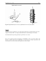

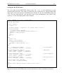
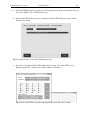
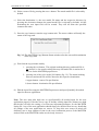
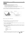
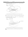
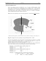
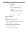
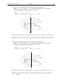
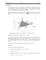
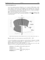
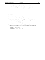
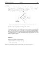
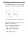
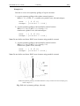
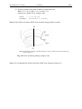
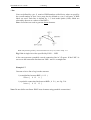
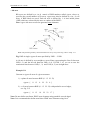
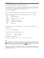
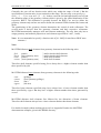
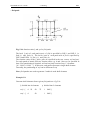
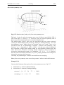
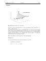
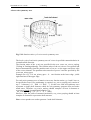
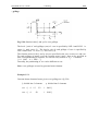
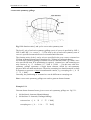
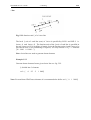
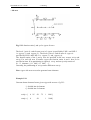
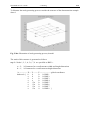
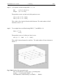
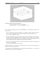
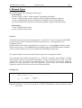
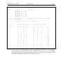
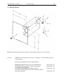
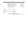
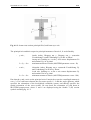
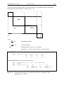
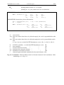
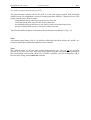
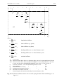
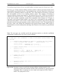
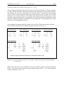
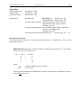
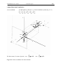
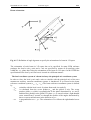
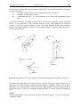
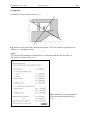
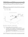
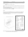
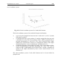
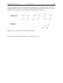

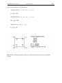
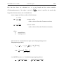
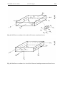
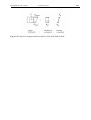
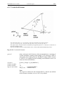
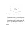
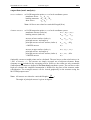
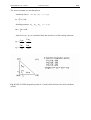
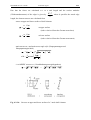
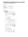
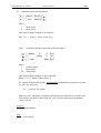
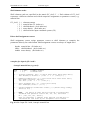
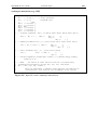
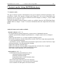
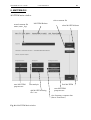
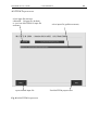
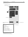
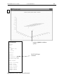
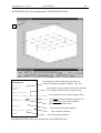
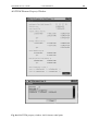
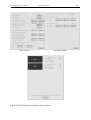
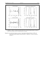
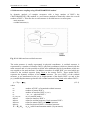
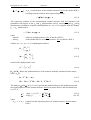
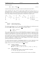
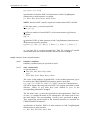
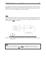
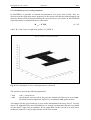
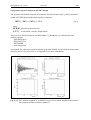
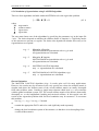
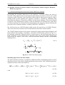
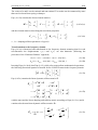
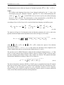
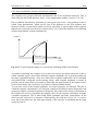
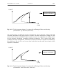
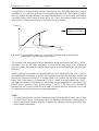
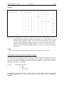
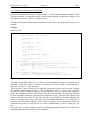


![[U3.01.00] Description du fichier de maillage de Code_Aster](http://vs1.manualzilla.com/store/data/006352534_1-e4fd209025fb7c0ab8d5dd0118ddbb98-150x150.png)


![[U3.14.09] Modélisation 3D_ABSO](http://vs1.manualzilla.com/store/data/006354556_1-90d294b391fedb0a3a4ef0c43d87b2dc-150x150.png)
![[U3.14.01] Modélisations 3D et 3D_SI mécaniques](http://vs1.manualzilla.com/store/data/006353306_1-ee66ca199d5dc34d37fc69c57c8e21ef-150x150.png)