Download PixeLINK µScope User`s Guide

PixeLINK µScope User’s Guide
Issue date: April 21, 2009
2
PixeLINK
3030 Conroy Road
Ottawa, Ontario, Canada
K1G 6C2
PixeLINK µScope© IMT i-Solution Inc . All rights reserved.
This manual is a part of PixeLINK µScope
Information in this document is subject to change without notice. No part of this document may be
reproduced or transmitted in any form or by any means, electronic or mechanical, for any purpose,
without the express written permission of IMT i-Solution Inc.
2
3
Contents
Contents .................................................................................................................................... 3
Introduction ............................................................................................................................... 7
PROGRAM GENERAL FEATURES AND FUNCTIONS ................................................................................... 7
MAIN TASKS ......................................................................................................................... 7
Chapter 1 - Getting Started .......................................................................................................... 9
OVERVIEW ........................................................................................................................... 9
USING THIS MANUAL ................................................................................................................ 9
Special conventions.......................................................................................................... 9
SYSTEM REQUIREMENTS .......................................................................................................... 10
SOFTWARE PACKAGE .............................................................................................................. 10
INSTALLING THE PROGRAM ........................................................................................................ 10
STARTING THE PROGRAM .......................................................................................................... 10
UNINSTALLING THE PROGRAM .................................................................................................... 11
Getting Technical Support ............................................................................................... 11
Chapter 2 - Image Processing ..................................................................................................... 12
WHAT IS IMAGE PROCESSING ..................................................................................................... 12
IMAGES AND IMAGE DIGITIZATION .............................................................................................. 12
PIXEL DEPTH ....................................................................................................................... 12
COLOR AND COLOR MODELS ..................................................................................................... 13
Gray Model ................................................................................................................... 13
RGB Model .................................................................................................................... 14
YUV Model .................................................................................................................... 14
HSB Model .................................................................................................................... 14
Program Specialty.......................................................................................................... 15
Converting between different color models ........................................................................ 15
IMAGE ENHANCEMENT ............................................................................................................. 15
Intensity modifying ........................................................................................................ 15
Spatial Filtering ............................................................................................................. 17
Chapter 3 - Program Basics ........................................................................................................ 19
OVERVIEW OF PROGRAM BASICS ................................................................................................. 19
PROGRAM LAYOUT ................................................................................................................. 19
Main window ................................................................................................................. 19
Toolbars ....................................................................................................................... 20
Menu Bar...................................................................................................................... 22
Status Bar .................................................................................................................... 22
Context window............................................................................................................. 23
ZoomIn window............................................................................................................. 24
Document window ......................................................................................................... 24
DOCUMENTS ....................................................................................................................... 27
Image document ........................................................................................................... 28
WORKING WITH DOCUMENTS ..................................................................................................... 28
Making a new document ................................................................................................. 28
Opening document......................................................................................................... 28
Opening recent documents.............................................................................................. 28
Reload document ........................................................................................................... 28
Closing document .......................................................................................................... 28
Saving document ........................................................................................................... 29
Saving document with new name ..................................................................................... 29
WORKING WITH COMMANDS ...................................................................................................... 29
Commands and menus ................................................................................................... 29
Interactive Commands.................................................................................................... 29
OPTIONS AND SETTINGS .......................................................................................................... 30
General tab................................................................................................................... 30
Measurement tab........................................................................................................... 31
Excel tab ...................................................................................................................... 33
Sequence tab ................................................................................................................ 33
Chapter 4 - Working with Images ................................................................................................ 35
SUPPORTED FILE FORMATS ........................................................................................................ 35
OPENING IMAGES .................................................................................................................. 36
Preview mode ............................................................................................................... 36
CREATING A NEW IMAGE .......................................................................................................... 38
CLOSING IMAGES .................................................................................................................. 38
Reload ......................................................................................................................... 39
SAVING IMAGES ................................................................................................................... 39
3
4
PRINT ................................................................................................................................40
PRINT PREVIEW .....................................................................................................................40
PAGE SETUP .........................................................................................................................40
EXPORT TO EXCEL ..................................................................................................................40
Chapter 5 – Edit Menu ................................................................................................................41
UNDO ................................................................................................................................41
REDO ................................................................................................................................41
COPY ................................................................................................................................41
PASTE ...............................................................................................................................41
PASTE NEW .........................................................................................................................41
DELETE ..............................................................................................................................41
DELETE ALL….......................................................................................................................41
ANNOTATING IMAGES ..............................................................................................................42
Line ..............................................................................................................................43
Spline ...........................................................................................................................44
Polyline .........................................................................................................................44
Rectangle ......................................................................................................................45
Ellipse ...........................................................................................................................46
Text label ......................................................................................................................47
Changing annotations......................................................................................................48
IMAGE INFO .........................................................................................................................48
File tab..........................................................................................................................48
Image tab .....................................................................................................................49
Calibration tab ...............................................................................................................49
Chapter 6- Acquiring Images .......................................................................................................50
Getting images from a Video or Digital Camera ...................................................................50
Live measurements.........................................................................................................52
Chapter 7 - Images ....................................................................................................................56
Changing image color models ...........................................................................................56
Changing image pixel depth .............................................................................................56
Show image in the view...................................................................................................57
DUPLICATING IMAGES ..............................................................................................................57
CROPPING IMAGES..................................................................................................................57
COPYING AND PASTING IMAGES ...................................................................................................57
Copy.............................................................................................................................57
Paste ............................................................................................................................57
Paste new......................................................................................................................58
Resizing images..............................................................................................................58
Rotating images .............................................................................................................58
Apply Vectors to images ..................................................................................................59
WORKING WITH IMAGE SEQUENCES ...............................................................................................59
USING AN IMAGE HISTOGRAM .....................................................................................................60
Histogram window ..........................................................................................................60
Chapter 8 - Process ....................................................................................................................63
SPATIAL FILTERING.................................................................................................................63
Edge filters tab...............................................................................................................64
Enhance filters tab ..........................................................................................................65
Morphological filters tab...................................................................................................67
Special filters tab............................................................................................................68
IMAGE ENHANCEMENT ..............................................................................................................68
Intensity modifying .........................................................................................................68
PSEUDO-COLORING IMAGES .......................................................................................................71
SHADING CORRECTION ............................................................................................................74
Chapter 9 - Measuring and Counting .............................................................................................75
CALIBRATION .......................................................................................................................75
Spatial Calibration dialog .................................................................................................75
Modify existing calibration................................................................................................77
Creating a new calibration................................................................................................78
Save and load calibration .................................................................................................81
Marker ..........................................................................................................................81
Split marker...................................................................................................................82
TAKING MANUAL MEASUREMENTS ................................................................................................83
Manual Measurements types ............................................................................................83
Visualizing measurements data.........................................................................................87
MANUAL TAGGING AND COUNTING ................................................................................................88
Visualizing manual tags data ............................................................................................88
4
5
PROFILE ............................................................................................................................ 89
Working with Profile lines ................................................................................................ 89
Graph properties for a line .............................................................................................. 90
Export to Excel .............................................................................................................. 91
EXPORTING MEASUREMENT DATA ................................................................................................. 91
Chapter 10 - Printing ................................................................................................................. 92
Page Settings ................................................................................................................ 92
Zooming In and Out ....................................................................................................... 93
Fit to window ................................................................................................................ 94
Fit to page .................................................................................................................... 94
WINDOW ........................................................................................................................... 94
Chapter 11 - Tools and Commands Reference................................................................................ 95
FILE MENU .......................................................................................................................... 95
New Image... ................................................................................................................ 95
Open............................................................................................................................ 95
Reload ......................................................................................................................... 95
Save ............................................................................................................................ 95
Save As........................................................................................................................ 95
Print... ......................................................................................................................... 96
Print preview................................................................................................................. 96
Page setup.................................................................................................................... 96
Export to Excel .............................................................................................................. 96
Export to Excel gray image data....................................................................................... 96
Preferences… ................................................................................................................ 96
Exit.............................................................................................................................. 96
Recent Files .................................................................................................................. 96
EDIT MENU ......................................................................................................................... 97
Undo............................................................................................................................ 97
Redo ............................................................................................................................ 97
Copy ............................................................................................................................ 97
Paste ........................................................................................................................... 97
Paste New .................................................................................................................... 97
Delete .......................................................................................................................... 97
Delete All… ................................................................................................................... 97
Annotate ...................................................................................................................... 98
Information................................................................................................................... 99
ACQUIRE MENU .................................................................................................................... 99
Image capture............................................................................................................... 99
Live measurements ........................................................................................................ 99
Overlay settings ...........................................................................................................100
Get image from PTP camera ...........................................................................................100
IMAGE MENU ......................................................................................................................100
Mode ..........................................................................................................................100
Clone ..........................................................................................................................101
Resize... ......................................................................................................................101
Rotate.........................................................................................................................101
Apply vectors ...............................................................................................................102
Sequence ....................................................................................................................102
Histogram… .................................................................................................................103
PROCESS MENU ...................................................................................................................103
Filters... ......................................................................................................................103
Brightness/Contrast... ...................................................................................................103
Pseudo-color... .............................................................................................................103
MEASURE MENU ...................................................................................................................103
Calibration ...................................................................................................................104
Manual measurements...................................................................................................104
Send statistics to Excel ..................................................................................................106
Manual tag...................................................................................................................106
VIEW MENU .......................................................................................................................106
Zoom In ......................................................................................................................107
Zoom Out ....................................................................................................................107
Zoom 100%.................................................................................................................107
Zoom ..........................................................................................................................107
Fit to Window ...............................................................................................................107
Fit to Image .................................................................................................................107
View type ....................................................................................................................107
5
6
Status Bar ................................................................................................................... 107
Context window............................................................................................................ 107
ZoomIn window............................................................................................................ 108
WINDOW MENU ...................................................................................................................108
Cascade ...................................................................................................................... 108
Tile Horizontal .............................................................................................................. 108
Tile Vertical..................................................................................................................108
Arrange Icons .............................................................................................................. 108
Split Horizontal............................................................................................................. 108
Split Vertical ................................................................................................................ 108
Close ..........................................................................................................................108
Close All ......................................................................................................................109
Next ...........................................................................................................................109
Previous ...................................................................................................................... 109
HELP MENU ........................................................................................................................109
About..........................................................................................................................109
Appendix A - GUARDANT ELECTRONIC KEYS. DIRECTION FOR USE. .............................................. 110
GENERAL PROVISIONS............................................................................................................110
USB PORT ........................................................................................................................110
RUNNING AND STORAGE REGULATIONS .........................................................................................110
6
7
Introduction
Welcome to PixeLINK µScope, the image-processing program designed to capture, modify, enhance,
and measure digital images.
PixeLINK µScope is a 32-bit/64-bit application for Windows
98SE/ME/2000/XP/VISTA. We hope that our program will help you to solve a wide variety of imageanalysis problems. Please take the time to read through this manual so that you can take full
advantage of PixeLINK µScope's many features.
Note: This user guide assumes you have a working knowledge of your computer and its
operating conventions, including how to use a mouse and standard menus and commands. It
also assumes you know how to open, save, and close files. For help with any of these
techniques, please see your Windows documentation.
This section describes the program's general features and functions as well as the tasks that the
program can help you perform.
Program general features and functions
The program allows you to:
• load and save images in several graphical formats:
− bmp
− jpg
− tiff
− pсx
− gif
− tga
• load and save image sequences in the formats below, if
− avi
DirectX 7.0 or higher is installed:
− mpg
− mov
− img, rpt (the formats from the IMT program)
• acquire
gray-scale and color images directly through a PixeLINK image device that the program
controls, open images from files, and paste images from the clipboard
• enhance image quality
• type comments, draw graphics, and exchange graphics between images
• manually measure linear and angular values
• export measurement results to MS Excel for further processing
• print images and results of analysis
Main Tasks
The main task of the program is to help a user identify objects on images and to measure their
parameters.
The following steps will help you carry out this task successfully:
I. Capture an image or open the image or image sequence.
II. Enhance the image.
III. Measure the objects.
IV. Create and print a report.
7
8
8
9
Chapter 1 - Getting Started
Overview
This chapter describes the organization of this manual and introduces you to the program. It also
covers some basics about using the program, including:
• Using this manual
• System requirements
• Software package
• Installing the program
• Starting the program
• Uninstalling the program
• Getting help
Using this manual
This program User's Manual is designed to provide you with instructions on using the program to
measure and manipulate color and gray scale images. The chapters of the manual cover the following
topics:
•
Introduction describes what the program is and its features.
•
Chapter 1 describes the system requirements, how to install and uninstall the program, and
how to get help.
•
Chapter 2 contains a short overview of image processing.
•
Chapter 3 describes the program layout, setting options, terms and notions, and working
with documents.
•
Chapter 4 describes general settings, printer settings, and how to open, save, and print
image files.
•
Chapter 5 describes how to manipulate images (cut, copy, paste, etc.), transform images,
and annotate the image.
•
Chapter 6 describes how to acquire images, to measure the image on preview windows, and
to set the overlay mask.
•
Chapter 7 describes how to manipulate, turn, divide, and merge images, and how to make
video files.
•
Chapter 8 describes various ways to control and enhance the quality of images.
•
Chapter 9 describes how to define image objects, measure image objects, view and process
data.
•
Chapter 10 describes how to print images, and measure results.
•
Chapter 11 describes all of the menu commands.
•
Appendix A describes the Guardant electronic key and how to use it.
Special conventions
Below are some special conventions used to present information in this manual. This special
information can help you to quickly solve possible problems while working with this program.
Important notes
Important notes and notices are marked like this:
Note: An important note.
9
10
Tips
Tips that can help you work with the program more efficiently are marked like this:
Tip: Useful tip.
Terms and Notions
Terms and notions used in this manual are marked as in this example:
Image is a picture in a digital form, suitable for processing by a computer. It consists of figures that
are the values of color brightness.
Referencing Commands
The manual refers to commands in the following way:
Menu¾Sub-menu¾Command
For example, to show the Filter dialog from the Process menu, the manual would describe the
location of the command as: Process¾Filter…
System Requirements
• PC with a Pentium-class processor; Pentium 300MMX or higher recommended
• Microsoft Windows 98SE/ME/2000/XP/VISTA operating system
• 32 MB of RAM or more (128 MB recommended)
• 15 MB hard-disk space
• CD-ROM drive
• VGA or higher-resolution monitor; Super VGA recommended
• Microsoft Mouse or compatible pointing device
• USB- or LPT-port for hardware key (depends on delivery).
Software package
The software package includes the program software and documentation:
•
•
•
The program software CD
The PDF program User’s Guide
USB- or LPT-port hardware key (drivers are included).
The program software CD contains everything you need to install and run the program:
•
Sample image files.
Installing the program
The program must be installed from within Windows. To install the program:
1.
Place the program Setup CD into the appropriate CD drive.
2.
Run PixeLINK µScope.exe in the program Setup CD and follow the instructions. You can install
“CaptureDrivers.exe,” which is the driver for PixeLINK imaging devices that are controlled by its
own programs.
3.
Connect the “Dongle (Electronic key)” to a printer port or USB port of your computer. Then
Windows will find it by itself.
Starting the program
After the program is installed it is automatically included in the Windows programs list. To run the
program:
10
11
1.
2.
3.
4.
Click the Start button.
Select the Programs item.
Select the IMT > PixeLINK µScope item from the Programs list.
Run the program.
Uninstalling the program
Use the Add/Remove Programs in the Control Panel program group or Uninstall or change a
program in the Computer (depending on Windows) group to uninstall the program. You must use it
to remove the program completely from your system..
Getting Technical Support
The services of Technical Support is available to registered customers. To reach Technical Support,
please contact the below.
PixeLINK
3030
Ottawa,
Phone: +1 (613) 247-1211
Fax: +1 (613) 247-2001
www.pixelink.com
Conroy
Road
ON
K1G
6C2
ext 300 or: 1 (888) 484-8262 ext 300 (Eastern Time Zone)
11
12
Chapter 2 - Image Processing
This chapter is a brief introduction to the basics of image processing, including:
• What is image processing
• Image Digitization
• Pixel Depth
• Color & color models, converting between different color models
• Image Enhancement
• Measuring and Counting
What is image processing
Visual representation of an object or a group of objects can be considered an image. Image processing
is used to change the information within an image. To perform specific digital image processing, a
computer is used.
To do this, the image must be converted into numeric form. This process is known as Image
Digitization.
Images and Image Digitization
Image is a numeric form of picture, or bitmap. It is a result of a digitization process that divides a
picture into very small picture elements, or pixels, which are often 1/300th of an inch square or
less. In the computer, the image is represented by a two-dimensional array (or digital grid) of
pixels.
Pixel is the smallest picture element that describes the color and brightness of a single point of the
picture. Each pixel is identified by its position in the bitmap and is referenced from the upperleft position of the bitmap.
The quality of the digital image is determined by the resolution specified during digitization.
Resolution is a ratio of the number of picture points to a unit of the picture area. Usually resolution is
defined in dpi (dot per inch). Desired quality (and thus resolution) and original picture size
defines pixel quantity, and thereby the bitmap dimension. During digitization each pixel in the
image is individually sampled, and its brightness is measured and quantified. This measurement
result is a value for the pixel, usually an integer that represents the brightness or darkness of
the image at that point. This value is stored in the corresponding pixel of the computer's image
bitmap. When the image is digitized, the width and height of the bitmap are chosen and fixed.
Together, the bitmap pixel width and height are known as its spatial resolution.
Pixel Depth
Each pixel value is a number. In a computer a pixel is represented by an 8-, 16-, 24- or 48-bit
unsigned integer. The number of bits depends on the number of colors an image has.
Pixel values for an image that contains only black and white colors can be represented by a single bit:
0=black, 1=white.
In order to represent all the possible colors—approximately 16.7 million that might be found in a True
Color image—a pixel must be at least a 24- bit unsigned integer.
Pixel Depth, or bits-per-pixel (BP), is the number of bits used to represent the pixel values in an
image. The requisite value of Pixel Depth depends on the image and its quality. Pixel Depth can
also be called Color Depth.
Most images supports more than one level of bits-per-pixel, and therefore more than one level of
color. The more information is recorded for each pixel, the more shades and hues a file can contain.
The following table lists all of the bits-per-pixel ratios in the image that the program supports, and
shows the corresponding maximum number of colors.
Bits-Per-Pixel
Maximum
Number
of
12
13
Colors
1
2
4
16
8
256
16
32,768
or
65,536
(depends on format)
24
16,777,216
32
16,777,216
48
281,474,976,710,656
Pixel Depth of an image gives us the number of unique colors that can be contained within the image.
But it does not tell us what colors are actually contained within the image. Pixel Depth plus one of
several conventions determine color interpretation, which we call the Color Model.
Color and Color Models
How can we describe and process colors? Natural colors are compound and can possess millions of
tints which the human eye cannot even differentiate. For example, a black-and-white image can be
represented by only a single bit: 0=black, 1=white. Color ones may take 24 bits. That means more
than 16 million colors. Fortunately, most color tints consist of different combinations of basic colors.
That allows us to describe color mathematically and create Color Models.
Color Model is a mathematical model describing color based on several components. A Color Model
enables us to interpret a pixel value and define what color and brightness the point of the image
described by this pixel has.
There are three primary colors of light: Red, Green and Blue. All other colors are represented by a
mix of different proportions of these three primary colors.
These primary colors can be called color channels.
Color Depth is the number of bits used to represent the pixel’s color component values in an image.
Pixel Depth is equal to Color Depth Red + Color Depth Green + Color Depth Blue. For
example, for a 24-bit color image the Color Depth is 8, but for 16-bit gray image the Color
Depth is 16.
All images can be subdivided into two main classes:
• Black-and-white,
where all the image colors are shades of gray, from black to white. All the
possible colors can be described by a Gray Model.
• Color, where all possible colors can be described by RGB, HSB, YUV, and other models.
By using color models we can describe color tints.
Gray Model
A Gray Model can be described as a scale ranging from completely black to completely white (all
colors are shown only as shades of gray). This level of grayness or brightness is called grayscale. If,
in the Gray Model, one pixel is stored by 8 bits (1 byte), a pixel with a value of 0 will be completely
black, and a pixel with a value of 255 will be completely white (in this case Pixel Depth is 8 BPP). That
means 256 levels of gray—at least 56 levels more than a human eye can distinguish.
13
14
A Gray Model with a Pixel Depth equal 16 BPP uses 16 bits to store a pixel and provides 65,536 levels
of gray.
This model needs only one color channel to represent a grayscale image.
RGB Model
RGB means “Red, Green and Blue,” the three primary colors of light. If you mix different levels of each
primary color in definite proportions, you will get any desired color. In a True Color image (Pixel Depth
is 24 BPP), each pixel contains a 24-bit value, 8 bits per one color. These brightness values represent
levels within a 256-level scale, from 0 to 255. The first
sample, the Red, ranges from 0 (black) to 255 (brightest
red). The Green sample is the level of green (0-255), and
the Blue sample is the one of blue (0-255). Various
combinations of the Red, Green and Blue values allow us to
get 224 (over 16 million) colors.
Equal levels of Red, Green and Blue always generate a level
of gray.
This model has three color channels.
In the case that the image Pixel Depth is 48 BPP, each
color component will have a range from 0 to 65,535. It
allows you to work with a wide range of digital cameras
and scanners without loss of any information.
YUV Model
In this model and RGB signal is converted to a single luminance signal (Y). You can use the following
formula to get the best conversion result:
Y = 0.299 R + 0.587 G + 0.114 B,
where R, G, and B stand for the brightness of the respective color channels and the coefficients
express physiological qualities of human vision.
U and V stand for color signals:
U = B – Y, V = R – Y
The three components described above are used in YUV model to express color.
This model has three color channels.
HSB Model
The HSB (Hue, Saturation, and Brightness) color model describes three fundamental characteristics of
color:
• Hue is the color reflected from or transmitted through an object. It is specified by a position on
the standard color wheel given as an angular displacement ranging from 0 to 360 degrees. In
common use, hue is identified by the name of the
color such as red, orange, or green.
• Saturation
(percentage of white in a color) is the
strength or purity of a color. Saturation represents
the amount of white in proportion to the hue,
measured as a percentage from 0% (white) to 100%
(fully saturated). Colors with the maximal saturation
(100%) are placed at the edge of the circle. By
decreasing saturation we make the color lighter, as if
white color was added. Every color with the minimal
saturation (0%) becomes white.
14
15
• Brightness
is the relative lightness or darkness of a color, usually measured as a percentage
from 0% (black) to 100% (white). By adjusting brightness we can add black color to the spectral
hue. Adding black and white, we create colors.
Complementary colors are placed opposite each other on the color circle, and every color is placed
between the colors it was made of. For example, blue and red together create magenta. To get the
increased intensity of a color we need to decrease the intensity of its complementary color. For
example, to modify the overall color towards green tints, we need to decrease the content of red.
This model has three color channels.
Program Specialty
This program supports Gray, RGB, HSB and YUV color models. It also supports the following values
for Pixel Depth:
• 8, 12, 16 – for Gray Scale images
• 24, 32, 48 – for color images
Depending on the chosen Pixel Depth, pixels are represented by 8-, 12-, 16-, 24-, 32-, or 48-bit
unsigned integers.
Note: An image with 16 bits per color channel can be saved only in the native file format
(*.img) and tif.
You will find the description of various file formats in Chapter 4 - Working with images.
Converting between different color models
The program allows you to convert images from one color model to another. During this operation,
the L*A*B color model is used as an intermediate format. It uses 16 bit values to provide lossless
converting.
Note: When decreasing Pixel Depth or converting a color image to a grayscale image you can
loose information, which will be impossible to restore later.
Image Enhancement
One of the main tasks of image processing is Image Enhancement. Its aim is to change the image so
that it will be possible to identify the objects on it most precisely. Object identification is usually
provided by binarization, or thresholding, which divides an image into objects and background. The
more the objects differ from the background in brightness and color, the more exactly they can be
thresholded. That is what image processing investigates. There is no general solution to this task for
all kinds of images, so this problem is solved empirically for each separate image.
There are several methods of image enhancement. One of them is to modify the intensity of each
pixel of an image.
Intensity modifying
The first way to enhance an image is to change the way intensity values are interpreted. For example,
if your image was very dark overall, you could boost all the values by a certain amount. You might
boost all values by 20 points, or flatten a range of intensities to a single value (e.g., set all intensities
from 75 through 127 to the same value of 150).
The following intensity manipulation tools are described here:
•
•
•
•
•
Brightness
Contrast
Gamma
Histogram
Thresholding
15
16
Brightness
Brightness (or intensity) describes the overall amount of light in an image.
For a digital image, the brightness of each pixel and the color model of the image are determined by
the pixel values.
For example:
• For a grayscale image, the brightness of a pixel is the pixel value.
• For an HSB image, the brightness of a pixel is the B component.
• For
an RGB image,
0.3*R+0.59*G+0.11*B.
the
brightness
of
a
pixel
is
expressed
by
the
formula:
When you increase brightness you increase the value of every pixel in the image, moving each pixel
closer to the intensity upper limit (for grayscale 8 BPP image this value is 255, or white). When you
decrease brightness you reduce the value in each pixel, moving it closer to the intensity lower limit
(for grayscale 8 BPP image this value is 0, or black). To the human eye, increasing or decreasing the
image brightness looks like decolorizing or darkening of the image, respectively.
For more details about modification of image brightness and how to do it, see Chapter 4 - Working
with images.
Contrast
Contrast denotes the degree of difference between the brightest and darkest components in an
image, i.e. the width of the image's brightness range.
An image with good contrast is composed of a wide range of brightness values from black to white. An
image with poor contrast contains only harsh black and white transitions, or contains pixel-brightness
values within a narrow range.
The amount of the intensity scale used by an image is called its dynamic range.
Thus we can tell that an image with good contrast will have a good dynamic range.
Modification of image contrast is modification of image dynamic range correspondingly. In other
words, on modification of image contrast each pixel value is scaled by a contrast value, which serves
to redistribute the intensities over a wider or narrower range. Increasing the contrast spreads the
pixel values across a wider range, while decreasing contrast squeezes the values into a narrower
range.
You will learn how to modify image contrast in Chapter 4 - Working with images.
Gamma
Gamma correction is a specialized form of contrast enhancement. It is designed to enhance contrast
in very dark or very light areas of an image by changing the midtone values, particularly those
at the low end, without affecting the highlight and shadow points.
Gamma is a parameter of the gamma correction function. When you reduce gamma value the image
gets darker and the contrast of light image details is increased. When you increase gamma
value the image gets lighter and the contrast of dark image details is increased.
Gamma correction can be used to improve the appearance of an image, or to compensate for
differences in the way different input and output devices respond to an image.
You will learn how to use Gamma Correction in Chapter 4 - Working with images.
Histogram
A Histogram (or Intensity Histogram) of an image is the distribution of intensities of individual
pixels. Usually a histogram is represented in a graphic form as a plot, where the X-axis
represents the intensity scale, and the Y-axis measures the number of pixels in the image
possessing that value.
16
17
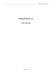
Here is an example of an Intensity Histogram:
Figure 2.1. An example of a Histogram.
Histograms measure and illustrate in graphic form brightness and contrast characteristics of an image.
Histogram data can be created and viewed for data gathering and analysis (discussed in more details
in Chapter 4 – Working with Images), or can be manipulated for image enhancement.
When you are working with grayscale 8 BPP images, the X-axis represents gray values from 0 to 255.
For grayscale 16 BPP images, the X-axis will represent the intensity range from 0 to 65,535. When
working with color images, you can choose to measure either the combined image luminosity or its
separate color channels (e.g., Red or Green or Blue, Hue or Saturation or Brightness...).
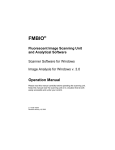
The Histogram allows you to estimate quickly what kind of brightness or contrast deficiencies exist in
an image. Figures 2.2.x show histograms for images with low contrast. You may see that histograms
are clustered around a very narrow portion of the color range. The position of the cluster will indicate
whether the image is too dark (see Figure 2.2.a), too light (see Figure 2.2.c), or simply too gray
(see Figures 2.2.b).
Figure 2.2.a. Dark.
Figure 2.2.b. Gray.
Figure 2.2.c. Light.
Brightness, contrast and gamma adjustments modify the shape of a histogram as follows:
• Contrast operations affect the width of the histogram—compressing it when it is decreased, and
stretching it when it is increased.
• Brightness operation affects the X-axis position of the histogram shape (intensity scale).
• Gamma correction operation affects the width, the X-axis position, and the shape
of the
histogram. A decrease in gamma brings out features in the lighter area of the image by
stretching the histogram in the upper region. An increase in gamma stretches the lower values,
providing increased contrast in the darker areas.
For more details about image histograms, see Chapter 4 - Working with Images
Spatial Filtering
If you want the objects of interest in the image to be thresholded well, it is necessary that the image
is “good”, i.e., image areas occupied by the objects of interest must differ from the other part of the
image on intensity.
Unfortunately ideal images are a rare thing in real life. Very often images contain areas in which the
intensity changes too quickly or too little, or contains areas of equal intensity with different colors and
other defects. Frequently people clearly see objects on the image but the program can not distinguish
them from the background, or does it poorly.
Filtering operations produce their effect by modifying a pixel's value (intensity) based upon the values
of the pixels that surround it. This small region is called pixel neighborhood.
17
18
Neighborhood is a square region of image pixels (typically 3x3, 5x5 or 7x7 in size) that surrounds
the specified pixel.
Filtering operations are used to even out or remove the image background, to identify the object
edges, to increase image sharpness, or to blur it.
Filtering is an operation that modifies the value for all pixels of the image based upon the values of
the pixels that surround it (pixel neighborhood).
All filters are divided into two categories:
• convolution (linear) filters,
• non-convolution (nonlinear) filters.
• edge filters
• special filters
Convolution filters
A convolution (or enhancement) filter has a kernel. A filter’s kernel is a matrix of filtering coefficients
(integer values). The size of a kernel defines the neighborhood size that the filter works with.
Convolution filters process each pixel neighborhood by multiplying the values within a neighborhood
by the filter’s kernel. The results of this multiplication are summed and divided by the sum of the filter
kernel. The result replaces the center pixel in the neighborhood of this pixel.
Usually this group contains filters to equalize the image histogram, perform image blur or sharpening,
and subtract image background.
Non-Convolution filters
Non-convolution (or Morphological) filters also work with the pixel neighborhood, but do not have a
kernel. These filters work only with data in the neighborhood itself. Applying to each neighborhood
either a statistical method or a mathematic formula gives a value that replaces the center pixel in the
neighborhood of this pixel.
You can find more details about image filtering in Chapter 4 – Working with Images.
18
19
Chapter 3 - Program Basics
Overview of Program Basics
This chapter reviews some basic parts of the program’s user interface, including:
• The program layout
• Options and settings
• Working with documents
• Working with commands
• The program menu structure
Program layout
The first thing you'll see when you run the program is the application's Main window. Initially this
window is relatively empty, as you can see in Figure 3.2, but once you start working, it will contain
one or more "child" windows displaying images, measurements, reports, etc.
Here is an example of the Main window containing several child windows:
Figure 3.1. program layout example.
Main window
The Main window is the main window of the program. It is shown on Figure 3.2. It contains a Menu
Bar, Toolbars, and Status Bar. The Main window can have "child" windows inside that display the
contents of Documents. These are called Document windows. Upon closing the Main window, the
program finishes its work. In the same figure, on the right, inside the Main window you will find the
Context window, which is described below.
19
20
Figure 3.2. The Main window.
Toolbars
A Toolbar is a set of buttons that represent the program tools (Figure 3.3). Press a toolbar button to
start the needed command. There are eight toolbars in the program. They are the Manual,
Annotate, Profile, Sequence, and Standard Toolbars. The program toolbars look and behave like
the ones in MS Internet Explorer, as follows:
• You
can find all the toolbars at the top of the Main window. If they are partially overlapped, a
“chevron” appears on a toolbar. Click on it, and you will find the latent part of the toolbar (Figure
3.3).
20
21
Figure 3.3. Toolbar’s partial covering.
• They can be moved close to the top edge of the Main window.
• Toolbars buttons can be in one of three states:
− Normal – the command is allowed, i.e. it can be performed. In this case a black-and-white
picture is displayed on the button (see Figure 3.4);
− Hot – the command is allowed. The mouse cursor is on the button, and a color picture is
shown on it (see Figure 3.4);
− Disabled - the command is forbidden, i.e. it cannot be performed. In this case a disabled
(gray) picture is displayed on the button (see Figure 3.4).
Hot
Normal
Disabled
Figure 3.4. The Toolbar’s button states.
• All
tools except Standard can be displayed or be hidden. The Standard toolbar is always
displayed. Click the right mouse button in the toolbar area at the top of the Main window to call
the Toolbar’s Context Menu. Then choose the toolbar name that you want to display or hide (see
Figure 3.5).
Figure 3.5. The Toolbar’s context menu.
• You may customize all the toolbars to include one or all of the tools associated with that particular
bar. To do it you need to display Toolbar’s Context Menu and select the Customize… tool. The
Customize Toolbar dialog will be displayed (see Figure 3.6). The Customize Toolbar dialog allows
you to display or hide the text labels of the toolbar buttons and to choose the button picture size
(small or large). The default size of icons is large.
Figure 3.6. The Toolbar’s Customize dialog.
21
22
Some toolbar buttons have an additional dropdown menu for fast access to often-used features. This
menu appears by pressing the arrow on the right side of the toolbar button. For example, in the
File¾Open…
command the dropdown menu contains a list of recently opened files.
Menu Bar
The Menu Bar is a specialized Toolbar. Press its buttons to call the list of commands available to
perform actions inside the program (see Figure 3.7). The structure of the Menu is described in
Chapter 7 – The Menu Structure.
Figure 3.7. An Example of the drop-down menu.
Status Bar
The Status Bar is located at the bottom of the Main window (see Figure 3.8). It displays several
panes:
• active-image calibration name
• active-image color model and color information about a pixel under the
is over an image
pointer, when the pointer
• pointer coordinates (in pixels), when the pointer is over an image
• active-image dimension
• active-image Pixel Depth
It also displays summaries of menu commands when the menu is active and the pointer is over a
command. The right mouse click in the Status Bar area will display the context menu, which allows
you to show/hide any pane (you can see an example of this menu in Figure 3.8).
Figure 3.8. Status Bar’s Context Menu.
The left part of the Status Bar can show a progress-bar indicator. This control is displayed only when
a long operation is executed, for example during the loading of a large file. The progress bar
represents the progress of operation and may display additional information about executed
operation. Figure 3.9 shows an example of a progress bar.
22
23
Figure 3.9. An example of a progress bar indicator.
Use the View¾Status Bar command to show or hide the Status Bar.
Context window
The Context window (or Image Manager window) is a window that shows all the opened images. It
contains a set of buttons. Each button has a thumbnail of one image. If the image document has
several images, each of them will have its own button. Thus, the Context window includes thumbnails
of all the images, and it allows you to work with them more comfortably.
An example of the Context window is shown in Figure 3.10
Three images in one document
Active image
Report Template document
Figure 3.10. An example of the Context window.
The active document has a button with a yellow frame. If the image document has several images,
the buttons of these images also have yellow frames (see Figure 3.10). An image button displays as
"pressed" only when the active document window displays this image.
A button also has an image or document name. If the name is too long it is displayed only partially.
Place the mouse cursor above the button to display a tool tip with the name of the image.
Usually for an active image it is 1. If several images are selected, each of their buttons has its own
figure. These figures show the order of the selected images. To select some images and to specify the
order of the selected images, you need to click the left mouse button on the desired image buttons,
while holding down the [CTRL] key on the keyboard. You can use the same method to deselect the
images, and the figures will disappear from the image buttons. With the [SHIFT] key you can choose
several images at a time.
Figure 3.11 shows the Context window with three selected images.
Figure 3.11. Selected images in the Context window.
The Context window lets you activate any image by a left mouse-button click on the desired image
button. As a result, the whole image document becomes active, and its document window is shown
23
24
over all document windows. Regardless of how many images are contained in the image document,
the active image will be displayed in the document window.
The Context window can be resized by clicking and dragging the corners or sides of the window.
During this operation all the buttons inside the Context window will be rearranged. You can show or
hide the Context window by using the View¾Context window menu command.
ZoomIn window
ZoomIn window shows a zoomed-in part of the image under mouse pointer in the active document.
Information in this window is updated as the mouse moves.
Figure 3.12 shows an example of the ZoomIn window. The contoured pixel in the center of the
window indicates the mouse pointer position. Marking of this pixel is optional. It can be switched
on/off in the “General” tab of the “Preferences” dialog in the “File” option.
Figure 3.12. An example of ZoomIn window.
The ZoomIn window can be resized by clicking and dragging the corners or sides of the window. You
can show or hide the ZoomIn window by using the View¾ZoomIn window menu command.
Document window
Document window is a window that displays document contents (images, Report Template,
measured data, measured objects, annotations, and others). It also allows you to manipulate
document data.
Figure 3.13 shows an example of the document window of the Image document.
A document window is created at the moment a document is created. The document stays open as
long as its document window is open. Closing the document window closes the document. Only one
document is active at a time. The document with an active document window is the active document.
You will find more detailed information about documents and how to work with them below in this
chapter.
24
25
Figure 3.13. An example of document window.
The upper part of the document window contains a title bar. The left part of the title bar contains
the System Menu Button, the document name, and some additional information depending upon the
active view mode. The right part has the Minimize, Maximize and Close buttons (see Figure 3.13).
Click on the
Close button to close the window and free the memory used to store the document.
An alternate way to close the window is to click with the mouse on the System Menu Button. A
menu will drop down and you can then choose the Close menu item. You can perform the same
action by choosing the Window¾Close menu command or by pressing the [CTRL] + [F4] shortcut
key on the keyboard.
Maximize button to enlarge a window to its maximum possible size. In this case a
Click on the
document window will occupy the entire program workspace, and other document windows will be
invisible.
Click on the
Minimize button to reduce the window to an icon. Minimized windows are placed along
the bottom of the program workspace. You can restore a window size and position by clicking the
Minimize button or by double-clicking its icon.
Like any window, a document window can be moved by dragging its title bar. It also can be resized by
clicking and dragging the corners or sides of the window.
Since several documents can be opened simultaneously, several document windows can be displayed
in the program window. You can use the [CTRL] + [Tab] or [SHIFT] + [CTRL] + [Tab] shortcut
keys to activate the next or previous document window correspondingly. Another way to do the same
is to use the Window¾Next or Window¾Previous menu commands.
In the left bottom corner of the window there is the Horizontal Split Button. It allows you to split
the window horizontally into two parts. The Vertical Split Button is located in the right top corner of
the window. It allows you to split the document window vertically into two parts.
25
26
Document window splitting
Document window lets you display two or four parts of the document simultaneously, i.e. the
document window can be split into two or four parts, named Panes. Right after creation a
document window contains only one part (or pane).
An example of the document window split into two parts is shown in Figure 3.14.
Figure 3.14. An example of the document window split into two parts.
• The Horizontal Split Button (see Figure 3.13) splits the document window horizontally into two
parts. It is located in the left bottom corner on the horizontal scroll bar of the document window,
or its part, when the window is split.
• The
Vertical Split Button (see Figure 3.13) splits the document window vertically into two
parts. It is located in the right top corner on the vertical scroll bar of the document window.
To move the separating line of the document window, place the mouse cursor on the line. The cursor
will change its view depending on the type of the line. It can look like:
• a horizontal arrow when the document window is split vertically,
• a vertical arrow when the document window is split horizontally,
• a cross arrow when the document window is split into 4 parts.
Press the left mouse button and while holding it down move the line in the desired direction. Release
the mouse button to fix the line.
An alternate way to split a document window is to double-click with the mouse on the Horizontal
Split Button or Vertical Split Button. In any of these cases the document window will be divided
into two equal parts.
26
27
You can also use the Window ¾Split Horizontal or Window ¾Split Vertical menu commands to
perform this action.
To cancel the splitting of the document window, double-click with the left mouse button on the
separating line you want to remove, or place the mouse pointer on the separating line and move it
while holding down the left mouse button until it matches an image edge. If the window is split into
four panes, move the cross point of the separating lines to an image corner.
An alternate way to cancel document-window splitting is to double-click with the left mouse button on
the separating line you want to remove.
You can also use the Window¾Split Horizontal or Window ¾ Split Vertical menu commands to
perform this action.
Each pane can display its own part of the document and contains View Header, View, Vertical
Scrollbar, Horizontal Scrollbar and several buttons that allow you to change view mode.
Note: At any moment, for your convenience, only one pane can be active. An active pane has
an active View Header (marked by blue color in the figure) and active (not gray) view mode
buttons. This pane can get commands from the keyboard input.
Document Views
The main part of a document window or its part (split pane) is a View. There are several types of
View, each of which can display the document contents in different formats. It is possible to
switch the visible View type at any moment by clicking the View ¾ View type .
There are the following view types used for and Image document:
•
•
•
•
Image View
Manual View
Manual Tags View
Profile View
For a Report Template document there is only Report View.
Not all program commands are available for each type of View. All types of View will be described in
detail below in this manual.
Documents
The program is designed mainly for working with images, but while working with the program new
data may appear: measured objects, annotations, reports, enhanced images, measurement and
statistics data, etc. To save these data, use Document.
Document is a container with some data in it, for example one or more images, thresholded objects,
results of measurements, and results of statistical treatment of the measurements data.
The program supports two types of documents:
• Image Document allows you to work with images and data related to them, such as thresholded
objects, measurements results, and statistics.
The program can work with image sequences, but an "Image Sequence Document" does not exist.
Instead, the Image Document is used because it can contain several images loaded from one file. The
Image Document has enough functionality to replace an Image Sequence Document.
Each document has only one document window, functioning as follows:
• Document window is created during the last stage of the document creation.
• Document is closed as soon as the document window is closed.
• Document window allows you to manipulate the document contents.
27
28
It is impossible to work with document contents without a document window. The program is designed
with the use of MDI-architecture, and a document window is created as a MDI-child window. It allows
you to have several document windows in the program. But only one window can be active at any
moment (the active window has a keyboard input), if at least one document is opened. This means
several documents can be opened, but only one of them can be active.
A document that has an active document window is an active document.
You can see an example of document window in Figure 3.13.
Image document
The Image Document contains one or more loaded or captured images, results of their treatment,
and data related to them: image attributes, thresholded objects, measurements results, etc.
Note: if the Image document has several images, only one image or its part can be displayed
in the document window. To work with another image of this document you need to activate
it in the Context window.
Working with documents
Making a new document
Keyword: CTRL+N
Menu: File¾New image…
The File¾New image… command shows the “New image” dialog. Use this dialog to select the type
you want and then press the OK button or Enter key on the keyboard. If you want to stop this
command, press Cancel or Esc on the keyboard. If the dialog ends successfully, a new document
window will appear. A new image document contains a new image with basic size and color.
Tip: [CTRL]+[N] key on the keyboard allows you to perform the File ¾ New image… command.
Opening document
Menu: File¾Open…
The File¾Open… command shows the “Open” dialog. Using this dialog you can select the path and
file you want to load. This command allows you to load several files simultaneously. If the dialog ends
successfully and a new document (or documents) is created successfully too, the command will load
the file (or files) contents to the document (or documents).
Opening recent documents
The File menu lists names of recently used files. By clicking on a menu item with the corresponding
file name you can load recently used files. If this file is already opened, this command performs
nothing. Otherwise it chooses a document type based on the file extension, creates a new document,
and loads the file contents to this document.
Reload document
Use the File¾Reload command to reload the active document. This command shows a prompt to
ensure you want to reload the active document. If you confirm, it closes the active document and
opens it again. All previous changes of this document will be discarded.
Closing document
The Window¾Close command is used to close the active document by closing the document window.
If a document has unsaved changes, a prompt will be shown to ensure you want to save the
document before closing it, close it without saving, or cancel this command. Depending on your wish,
the command will break or execute its action.
28
29
Saving document
The File¾Save command is used to save the active document changes to a file. If the active
document is not saved yet, this command provides the same action as the File¾Save As… menu
command.
Saving document with new name
The File¾Save As… command is used to save the active document changes to a file with a new
name. It shows the Save As dialog, in which you can choose the path to save a file and type a new
file name. If the Save As dialog is ended successfully, the command will try to save a document with
the selected path and the new name. If this procedure is completed successfully too, the active
document will have the new name.
Working with commands
The program provides a lot of commands and tools that allow you to manage the program execution.
Each command performs some single action (loads a file, filters an image, etc.) or repeats its action
many times (draws a line, outlines an object, etc.). You can start a command by clicking a button on
the toolbar, by choosing a menu item, by pressing a key on the keyboard, or by other ways. Usually
the menu provides a full set of commands. The toolbars and the keyboard shortcuts give access to a
set of these commands; they provide an alternative way to start the commands.
Commands and menus
A menu is a list of menu items, and each menu item is a command. When you choose a menu item
the corresponding command is started. Most commands are available to execute only if certain
conditions are satisfied. The menu item state represents the command's availability. If the menu item
is disabled (gray) it means the corresponding command cannot be executed. For example, if a
document is not changed the File¾Save menu item is disabled, but the File¾Exit menu item is
always enabled.
Most of the menu items are prefaced by icons. You can also judge a command state by the state of an
icon.
You can find an example of the menu item states in Figure 3.15.
Figure 3.15. An example of menu item states.
Interactive Commands
Interactive commands are a set of commands designed to make one kind of work repeatedly, for
example, the Edit¾Annotate¾Line command. During execution of this command you can draw a
straight line on an image. To do it you need to click the left or right mouse button and move the
mouse pointer, i.e. this command is required to interact with a user. After the desired straight line is
drawn the command is restarted automatically because it can create only one straight line.
29
30
Command is interactive if it needs to interact with a user to perform its action. Usually interactive
commands are repeated until a user cancels them. An interactive command is also called a tool.
Command settings
Some interactive commands allow you to change their settings. These commands have one or more
tabs containing controls that let you change command settings. For example, the
Edit¾Annotate¾Line command has two tabs. The “Color” tab allows you to choose the Background
and Foreground colors of the drawn line. The “Figure” tab lets you change the styles of the line
endings and the line thickness. These tabs are included in the “Properties” tab dialog, which is
displayed until the command is executed. After the command is ended, these tabs will hide.
An example of the Edit¾Annotate¾Line command properties tab window is shown in Figure 3.16.
The Line annotation
The Edit¾Annotate¾Line
command settings window
Figure
3.16.
An
example
for the Edit¾Annotate¾Line command.
of
the
“Properties”
tab
window
Note: Some interactive commands cannot get new settings until restarted. If you want to
immediately apply new settings to such commands, you need to restart them manually.
Options and Settings
The program lets you customize general aspects of the program to your own specifications. You can
read about how to customize the toolbars above. Here are some other options that can be changed:
• colors of object contours and measurement contours
• measurement label colors
• measurement label contents
• depth of undo stack (number of commands that can be undone)
These changes can be done in the “Preferences” tab dialog. There are six different tabs that can be
opened and used to control the program. They are:
•
•
•
•
General tab
Measurement tab
Excel tab
Sequence tab
The complete description of each of these tabs is given below.
General tab
You can see an example of the “General” tab in Figure 3.17.
30
31
Figure 3.17. An example of “General” tab.
This figure shows the following:
• Undo
buffer size field allows you to specify the depth of the Undo stack (number of commands
that can be undone).
• Prompt
before closing modified images flag lets you indicate that the program can issue a
warning asking if you want to save a modified image before attempting to close it.
• Open
images fitted to screen flag lets you indicate that the program must adjust the
magnification and the window size of a just-opened image so that the entire image is displayed
in the window.
• Show calibration units in table headers flag influences the display of Object, Statistics and
Measurement views.
• Zoom
factor control allows selecting more appropriate magnification strength for the ZoomIn
window.
• Show mouse hot flag shows in the ZoomIn window the exact position of the mouse pointer on
the image.
• Digits after decimal point flag allows you to show digits after the decimal point. It can show up
to three digits after the point.
Measurement tab
You can see an example of the “Measurement” tab in Figure 3.18.
31
32
Figure 3.18. An example of “Measurement” tab.
This figure shows the following:
• Colors box contains three controls that allow you to specify the colors:
− Features control lets you specify the color that will be used to draw measurement features.
− Measurements control lets you specify the color that will be used to draw measurements.
− Labels control lets you specify the color that will be used to draw measurement labels.
− Back lets you see the background of the drawn measurement labels.
• Measurement
labels:
label box contains controls that allows you to specify contents of measurement
− Show measurement name lets you specify that measurement labels will display the
names of measurement features. If you select this field the Show measurement units
field is disabled.
− Show measurement value lets you specify that measurement labels will represent values
of measurements. If you select this field the Show measurement units field is enabled.
− Show measurement units lets you specify that measurement labels will display the units
of measurements together with the measurement values.
− Show measurement name and value lets you specify that measurement labels will
display the names of measurement features and the values of measurements at the same
time. If you select this field the Show measurement units field is enabled.
• Visibility box:
− Line thickness field specifies the object thickness of manual measurements.
− Font size shows the size of figures that show measurement values.
• Apply to image box:
− Line thickness field specifies the object thickness of manual measurements after Apply
vectors to the image command.
32
33
− Font size shows the size of figures that show measurement values after Apply vectors to
the image command.
Excel tab
You can see an example of the “Excel” tab in Figure 3.19.
Figure 3.19. An example of “Excel” tab.
This figure shows the following:
• Row
and Column of the starting cell in the Excel sheet where the program will transfer
information.
• Don’t send table’s header (data only) will transfer only the data to the Excel sheet.
• Put active manual measurement into focused cell will transfer manual measurement value to
the focused cell of Excel sheet.
Sequence tab
You can see an example of the “Sequence” tab in Figure 3.20.
33
34
Figure 3.20. An example of “Sequence” tab.
This figure shows the following:
• Compression allows you select an appropriate method of compression for a saved video stream.
• FPS (Frames per second) determines the speed of further playback of a saved video stream.
• Quality
control allows you to specify the desired power of the video compression while saving a
sequence to a file. Less quality yields smaller file size and worse video output.
34
35
Chapter 4 - Working with Images
Image manipulation is one of the main tasks of Image analysis, and the program provides a lot of
tools for modifying and transforming images. This chapter describes procedures ranging from simple
tasks such as copying, resizing, or rotating an image, to advanced tasks such as image filtering.
Supported file formats
The program supports several different image file formats. The number of colors that a file can contain
is determined by the pixel depth (bits-per-pixel): the more information is recorded for each pixel, the
more shades and hues a file can contain.
The table given below lists the image formats that are supported by the program, the type of support
that is provided (read, write, or both), and the format's bits-per-pixel levels.
Supported Image Formats:
Format
Sub-Format
or
Compression
BMP
RGB encoded
BMP
RLE encoded
GIF
Ver.87a
(interlaced)
Ver.87a
(noninterlaced)
Ver.
89a
(interlaced)
Ver.89a
(noninterlaced)
Huffman
compressed
GIF
GIF
GIF
JPG
= program can open files,
Source/Sta
ndard
CompuServe
Joint Photo.
Expert Group
PCX
Version 0
PCX
PCX
Ver.2
(with
palette
info)
Ver.3
(without
palette info)
Version 5
ZSoft
Paintbrush
ZSoft
Paintbrush
TGA
Compressed
Truevision
TGA
No compression
Truevision
TIFF
Huffman
compressed
Pack
bits
compression
LZW
compressed
No compressed
Aldus
Corporation
Aldus
Corporation
Aldus
Corporation
Aldus
Corporation
TIFF
TIFF
4
CompuServe
Joint Photo.
Expert Group
TIFF
1
CompuServe
Progressive
PCX
BPP and Color Type
Microsoft
Windows
Microsoft
Windows
CompuServe
JPG
= program can save files
ZSoft
Paintbrush
ZSoft
Paintbrush
35
8
Grey
8
Color
16
24
48
36
The table below lists the image-sequence formats that are supported by the program.
Type
AVI
File
extension
*.avi
MOV
*.mov
Apple Quick Time
MPEG
*.mpeg,
*.mpg
Compressed
Support
Comment
Standard Windows video format
The table below lists the native file formats that are supported by the program.
Type
Image
Document
Report Template
Document
File
extension
*.img
Support
*.rpt
Comment
This format is used to store the whole program Image
document.
This format is used to store the program Report
Template document.
Opening Images
When you select the File¾Open… menu or press the [CTRL] + [O] shortcut key on the keyboard,
the “Open” dialog box will appear. You can find an example of this dialog in Figure 4.1.
Figure 4.1. The “Open” dialog box.
Using this dialog you can select the path and file you want to load. It seems like a standard Windows
“Open” dialog box, but it has an important addition. The program “Open” dialog box has Preview
mode. You can toggle this mode by pressing the Preview Mode button that is placed on the right side
of the dialog toolbar.
Preview mode
When Preview mode is turned on, both the Preview pane and Information pane are visible. These
panes allow you to see images and get image information just before you load them. You can see
these panes on the right side of the dialog in Figure 4.1.
36
37
The Preview pane displays the single image that is contained in the selected image file. After you
select a new file in the dialog file list, the image will be displayed in the Preview pane. If the selected
file contains several images, only the first one will be shown in the Preview pane.
The Information pane displays information about the selected image:
• image dimension (width, height),
• color space (grayscale or RGB) and pixel depth,
• number of images in a file,
• file compression type,
• file size.
If you select several files in the dialog file list, the Preview pane and Information pane will be
empty.
Note: You can preview only the images that are contained in files with formats supported by
the program. The Files of type dropdown box includes the list of all supported file formats.
If you want to preview a big size file it may take some time to load an image. During the image
loading the progress indicator will appear on the bottom of the dialog box, as you may see in Figure
4.2.
Figure 4.2. The “Open” dialog box during the file loading for preview.
The File¾Open… command allows you to load several files simultaneously. If the dialog ends
successfully and a new document (or documents) is successfully created, the command will load the
file (or files) contents to the document (or documents).
Note: If the loaded image has a Pixel Depth or Color Model not supported by the program it
will be converted to the most suitable Pixel Depth or Color Model.
37
38
Creating a new Image
Use the File¾New Image… command to create an empty image of the specified dimensions and
color model. After you choose this command the “New Image” dialog box will appear. An example of
this dialog is shown in Figure 4.3.
Figure 4.3. An example of the “New Image” dialog box.
This figure shows the following:
• The Color Model control allows you to select a color model for a new image.
• Bit/Channel
allows you to specify the color depth for a new image. If you select the 16 radio
button the pixel depth will be 16 BPP for grayscale images or 48 BPP for color images; otherwise
the 8 radio button will remain selected, which means the pixel depth will take a value of 8 BPP for
grayscale images or 24 BPP for color images.
• The
Width edit box allows you to specify the new image width value in pixels. This value
establishes the number of pixels the new image will contain in the horizontal direction.
• The
Height edit box allows you to specify the new image height value in pixels. This value
establishes the number of pixels the new image will contain in the vertical direction.
• Press the OK button to create a new, empty image of the specified size and color model.
• Press the Cancel button to break the command execution.
When an empty image is created, all pixels are initialized with the highest intensity value for its type
(e.g., 255, or white, for a grayscale 8 BPP image).
After an empty new image is created the new document window will appear.
Tip: You can use the [CTRL] + [N] shortcut key to perform the File¾New Image… command
After an empty image is created, the image data can be copied into it using the Edit¾Paste
command.
Tip: You can use the Edit¾ Paste New command to create a new image from the contents of
the Windows Clipboard.
Closing Images
To close an active image and remove its window from the screen choose the Window¾Close menu
command, or click on the
Close button in the upper right corner of the image window. If the
active image document contains several images, all of them will be closed.
Note: If you have modified an image before attempting to close it, the program can issue a
warning asking if you want to save it first. Choose the File¾Preferences… command, which
will display the “Preferences” tab dialog. Set the appropriate flag in the “General” tab to issue
a warning. Otherwise, set the preference not to warn you, and your image documents will close
immediately with no changes and no warning.
38
39
Tip: You can do the same by pressing the [CTRL] + [F4] shortcut key.
Reload
This command restores a modified image to the original image. If you saved the image with the same
name as the modified image, the most currently saved image will appear.
Saving Images
Use the File¾Save command to immediately store the contents of the active document window to its
file (the file name is listed on the window title bar). After this command is executed the image and its
window remain active.
Tip: You can perform the File¾Save command by pressing the [CTRL] + [S] shortcut key on
the keyboard.
If the document window is untitled, it means the document is not saved yet, so the “Save As” dialog
box will appear. An example of this dialog box is shown in Figure 4.4.
Figure 4.4. The “Save As” dialog box.
You need to type the document name in the File name edit box and press the Save button to
continue the storing process.
You may also save your image in the specified format. To do this you need to choose the desired file
format from the Save as type dropdown box. This box contains the list of all image file formats that
are supported by the program.
The File¾Save command with *.img format saves the entire document and any document part, such
as images, measured data, and statistics data, as well as its images, as a single file.
39
40
Print
Use this command to print one or more copies of the active report, or the active document view, to
the selected output device. This command shows the standard “Print” dialog that lets you take full
advantage of your printer capabilities.
Print Preview
Use this command to preview the active report or the active document view before printing. This
command displays the “Print preview” dialog box that shows how the report pages will look before
you print them.
Figure 4.5. The “Print Preview” dialog box.
Page setup
Use this command to access the standard Windows “Page setup” dialog box for the printer you have
selected. You can change the page layout settings using the controls in this dialog, and change the
selected printer and its settings.
Export to Excel
Use the File ¾Export to Excel command to send to Excel information provided by a view. In the case
of Image View, common information about the image will be transferred. Performing this command on
‘preview’ allows you to transfer image data to Excel without capturing the image.
40
41
Chapter 5 – Edit Menu
Edit menu contains commands you need to work with images. You can use the Edit menu
commands to copy, crop, or paste all or part of images. The Edit menu also contains commands that
allow you to change print properties of images and to modify view windows and information about the
images.
Undo
To cancel the most recent commands, you can use the [CTRL] + [Z] command. The depth of the
undo stack defines the number of commands that can be undone. You can change this in the
“General” tab of the “Preferences” tab dialog, which can be displayed using the
File¾Preferences… command. Undo command allows the image to undo the most recent
commands. You can use this command to perform the previously undone commands (by the
Edit¾Undo command) again.
Redo
Perform again the previously undone commands.
Copy
Use the Copy ([CTRL] + [C]) command to copy the contents of the region of interest (ROI) of the
active image to the Window Clipboard. If the image has no ROI, the entire image will be copied to the
Clipboard. The Edit¾Copy command will not change the contents of the active image (i.e., this
command does not delete the copied pixels). Any data already existing on the Clipboard will be
replaced.
You can paste the copied data to any opened image using the Edit¾Paste command. You can also
create a new image directly from the Clipboard contents using the Edit¾Paste New command.
Paste
You can use the Paste ([CTRL] + [V]) command to retrieve data, images, or drawing objects from
the Windows Clipboard. Before you perform this command, you need to check whether the image data
exists on the Windows Clipboard (for more detail, see “Copy”). If you do not have the data on the
Clipboard, the Paste command will not work. You can paste all image data on the Clipboard to any
data format supported by the program. The program allows you to Paste *.bmp, and *.jpg format
images that are copied to Clipboard from other programs. However, it sends you an ‘error’ message
when the data is not image data but something else, such as text data, or spreadsheet data.
Paste New
By this command you can retrieve images or data from the Windows Clipboard and place them into a
new image.
Before you perform this command, you need to check whether the image data exists on the Windows
Clipboard (for more detail, see “Copy”). The Edit¾Paste New command is available only if the
Windows Clipboard has valid image data in it. You can place the image data into the Clipboard using
the Edit¾Copy command. After a new image is created, it becomes an active image. The pixel depth
and color model of the new image will be the same as that of the original image. If a nonrectangular
ROI or drawing object is copied into the Clipboard, the program uses its bounding box for the new
image.
Delete
Use this command to remove the selected objects from your image or report page.
Delete All…
This command shows the “Delete all objects” dialog box, which contains the types of objects that
may exist in your image. After you choose the types of objects you want to remove, and close this
dialog by clicking the OK button, the objects with the selected types will be deleted from your image.
41
42
Annotating images
This set of commands and tools contained in the Edit¾Annotate popup menu allows you to add text
labels, shapes, arrows, etc. on the image. The program lets you store your annotations (also known
as overlays) in the program's native format file. Once the annotations are inserted into your image,
you can change them. The annotations do not become a part of the image until you execute the
Image¾Apply vectors… command.
Annotation commands are as follows:
• Select: You can use this command to select an annotation object. After that you can change its
position or shape. You can also change the selected object properties using the “Properties” tab
window, which will be displayed when you select a single object. The number and contents of the
tabs depend on the object.
• Line: You can use this command to draw straight lines in the active image or in the active report
page. Using the settings of this command, you may define the following line properties: color,
width of your line, and types of end points of the line. Changing the types of the line end points
allows the straight line to look like an arrow.
• Spline:
This command allows you to draw closed or open-ended shapes outlined by a spline in
the active image or in the active report page. Using the settings of this command, you may define
the shape properties: background and foreground colors, width of contour, types of the end
points, and filling mode.
• Polyline:
This command allows you to draw a closed or open-ended polyline or a filled or thin
polygon shape in the active image or in the active report page. Using the settings of this
command, you may define the shape properties: background and foreground colors, width of
outline, types of the end points, and filling mode.
• Rectangle: Use this command to draw filled or thin rectangular shapes in the active image or in
the active report page. Using the settings of this command you may define the following shape
properties: background and foreground colors, width of contour, and filling mode.
• Ellipse: You can use this command to draw filled or thin elliptical shapes in the active image or in
the active report page. Using the settings of this command you may define the following shape
properties: background and foreground colors, width of contour, and filling mode.
• Apply
Vectors: This command makes already-drawn annotations, measurement objects, and
manual-measurement objects become permanent parts of the image, so that they cannot be
changed later. Go to Image¾ Apply vectors.
The above commands are available only in an Image View or in a Report View.
The Edit¾Annotate¾Select and Image ¾ Apply vectors commands require the presence of at least
one annotation object. The results of all these commands can be discarded by using the Edit¾Undo
command.
Each drawing object has several properties. You can change object properties during the object
creation process or later. The first six tools have a “Properties” dialog box, which is displayed while a
tool is executing. This dialog has several tabs that allow you to change object properties.
Note: All object properties that you change while the tool is executing will be applied to the
next created object. It means you need to change the object properties before it is drawn. It is
also possible to change the object properties after selecting it by using the Select command.
The Edit¾Annotate and Image¾Apply vectors commands do not have tabs.
The Edit¾Annotate¾Select command can display the “Properties” tab dialog only if one drawing
object is selected.
All the drawing objects have the "Color" tab. You can see an example of the "Color" tab window in
Figure 5.1.
42
43
Figure 5.1. An example of the "Color" tab window.
This figure shows the following:
• This tab window allows you to choose Background and Foreground colors of the drawn object. In
the left part of this window the currently selected colors are shown.
• The
middle part is the Palette, which contains color buttons. You can change the object
Background or Foreground color by clicking the right or left mouse button correspondingly on the
Palette color button. Double clicking the left mouse button on the Palette color button calls the
Windows “Choose Color” dialog, which can help you replace a color of this Palette button.
• The right part of the "Color" tab window contains switches. They allow you to choose the palette
you want to use: color or grayscale. You can see an example of the "Color" tab window with a
grayscale palette in Figure 5.2.
Figure 5.2. An example of the "Color" tab window with grayscale palette.
The other tab windows will be described below.
Line
The Edit¾Annotate¾Line command is used to draw straight lines and arrows on an active image.
To draw a line, you need to select this tool, then press the left or right mouse button on the location in
your image where you want to start the line. Then hold the mouse button down, drag the mouse
cursor to the desired ending point, and release the mouse button. As a result the line will appear.
The start and the end points of the line are marked by the endings. You can change styles of the line
endings to make an arrow from a line.
While the line tool is executing, the "Figure" tab is displayed in the “Properties” tab dialog. It allows
you to change styles of the line endings and the line thickness. You can find an example of the
"Figure" tab window in Figure 5.3
43
44
Figure 5.3. The "Figure" tab window for the Edit¾Annotate¾Line command.
This figure shows the following:
• The Line width control allows you to define the line thickness.
• The End styles controls allow you to change the styles of the line endings.
An example of an arrow is shown in Figure 5.4
Figure 5.4. An example of an arrow.
Spline
The Edit¾Annotate¾Spline command is used to draw an opened or closed spline line or spline shape
on the active image.
Spline shape is a figure that is created as a bicubic spline from the given reference points. The spline
shape is open if the start and end points of its contour are not equal; otherwise the spline shape
is closed.
The spline reference points are set by the mouse button clicks. To create a spline, click the left mouse
button at each point (including the beginning one). The spline edges will be drawn automatically
during spline creation. Double-click the left mouse button to close the figure.
The "Figure" tab window, which is displayed while the Edit¾Annotate¾Spline command is
executing, lets you change the spline properties: the spline contour thickness, styles of the opened
spline line ending, and filling mode for the closed spline shape.
The "Figure" tab window for the Spline command is the same as for the Edit¾Annotate¾Polyline
command. You can find an example of the "Figure" tab window in Figure 5.6 and in Figure 5.7.
The Closed flag on the "Figure" tab window turns your spline line into a closed spline shape. The
area limited by the spline contour is filled according to the Border/fill mode property.
In the example in Figure 5.5 you can see the opened and closed spline shapes.
Figure 5.5. An example of the opened and closed spline shapes.
Polyline
The Edit¾Annotate¾Polyline command is used to draw an open or closed polyline or polygon shape
on an active image.
The polyline is a figure that can include both straight line segments and smooth edges. The vertexes
are set by the mouse button clicks. To create a polygon, click the left mouse button at each vertex
(including the start point) in the polygon. Smooth edges are created by holding the mouse button
down while you are dragging the mouse cursor. Double-click the left mouse button to end the polyline.
44
45
The "Figure" tab window allows you change the properties for the polygon or polyline, including
polyline thickness and styles of the polyline ending.
You can find an example of the "Figure" tab window in Figure 5.6. and Figure 5.7.
Figure 5.6. The "Figure" tab window for Polyline and Spline.
This figure shows the following:
• The Line width control allows you to define the polyline thickness.
• The End styles controls let you change the styles of the polyline endings.
• The Closed flag turns your polyline into a closed polygon.
Figure 5.6 shows the "Figure" tab window when the Closed flag is not checked.
If the Closed flag is checked, the Polyline command produces the polygon that is the area limited by
the polyline just created. This area is filled according to the "Figure" tab window settings. You can see
an example of the "Figure" tab window with the Closed flag checked in Figure 5.7.
Figure 5.7. The "Figure" tab window for the Polygon and Spline shapes.
This figure shows the following:
• The Line width control allows you to define the polygon outline thickness.
• The Closed flag turns your polyline into a closed polygon.
• The Border/fill mode controls allow you to choose the polygon area filling mode.
You can see the polygon and polyline shapes in Figure 5.8
Figure 5.8. An example of the polygon and polyline shapes.
Rectangle
The Edit¾Annotate¾Rectangle command is used to draw a rectangle shape on the active image.
45
46
To draw a rectangle, place the mouse cursor in the desired position in the image and press the left
mouse button. Then, holding the left mouse button down, drag the mouse cursor for the appropriate
length and release the left mouse button. As a result the rectangle shape will appear.
The "Figure" tab window allows you to change the rectangle properties: the border thickness and the
filling mode.
You can find an example of the "Figure" tab window in Figure 5.9.
Figure 5.9. The "Figure" tab window for the Rectangle command.
This figure shows the following:
• The Line width control allows you to define the rectangle border thickness.
• The Border/fill mode controls allow you to choose the area filling mode.
An example of the rectangle shapes is shown in Figure 5.10.
Figure 5.10. An example of rectangle shapes.
Ellipse
The Edit¾Annotate¾Ellipse command is used to draw an elliptical shape on the active image.
To draw an ellipse, press the left mouse button in the desired location on the image. Then, holding the
left mouse button down, drag the mouse cursor until an ellipse of the size and shape you need is
produced, and release the left mouse button.
The "Figure" tab window for the Edit¾Annotate¾Ellipse command is the same as for the
Edit¾Annotate¾Rectangle command. It allows you to change the ellipse shape properties: the
border thickness and the filling mode. You can find an example of the "Figure" tab window in Figure
5.9
An example of the ellipse shapes is shown in Figure 5.11
Figure 5.11. An example of ellipse shapes.
46
47
Text label
The Edit¾Annotate¾Text label command is used to place text on the active image.
To draw the text you need to select the Edit¾Annotate¾Text label command first. Then click the left
mouse button inside the image. While this command executes you will see an empty text box and the
“Properties” tab dialog with several tabs. After you release the left mouse button the “Text” tab will
be active. After you enter the text on the “Text” tab and set its attributes and colors on the
“Settings” and “Color” tabs, click the right mouse button anywhere on the image to finish this
command.
The “Settings” tab window lets you select the text characteristics, such as type font, size, style and
alignment, as well as special attributes such as bold, italic, or underlined.
Note: all these attributes are applied to the entire character string that will be applied to the
image.
An example of the "Settings" tab is shown in Figure 5.12
Figure 5.12. The "Settings" tab window.
Here the following properties are set:
• Font by which the text will be drawn and its attributes.
• Text Alignment in the rectangle surrounding it.
• If the Word wrap flag is checked, and the text cannot be placed in one line, it is automatically
continued on the next line as soon as it reaches the edge of the bounding rectangle.
• Transparent lets the image show through a drawing on top of it. If this flag is not set, the text is
enclosed in a box filled by the Background color.
• The Autosize bounds flag lets the rectangle enclosing the text change as the text changes.
• Alignment allows you to align the arrangement of the text.
An example of the "Text" tab is shown in Figure 5.13.
Figure 5.13. The "Text" tab window.
Here the text that will be displayed is set. An example of the text labels is shown in Figure 5.14.
47
48
Figure 5.14. An example of text labels.
Changing annotations
The Edit¾Annotate¾Select tool lets you select an annotation object from the earlier-drawn ones on
the image. This command can select only objects that are not “burned” into the image (not a
permanent part of the image). While an object is selected, its reference points are marked by white
squares. Using this command, you may also select more than one object by holding down the [CTRL]
key on the keyboard while clicking the mouse pointer on the objects. It is possible to select all the
objects in an area by using the object selector to draw a rectangle to enclose the objects.
You may change all the annotation objects that are not “burned in.” To do this, select the desired
objects first, using the Edit¾Annotate¾Select tool. After the object reference points are drawn by
white squares, you can change the object by dragging these points. You may also move the whole
selected object or several selected objects by dragging any part of any selected object excluding
reference points.
If you select only one object the “Properties” tab dialog with object-dependent tabs will be displayed,
otherwise this dialog will be hidden. These tabs allow you to change object properties in the same
manner as during object creation.
The menu commands Edit¾Copy and Edit¾Paste can be used to manipulate the selected objects.
These commands allow you to copy the selected annotations to the Windows Clipboard and paste a
new copy of them to the active image. You can perform the same actions by using the [CTRL] + [C]
and [CTRL] + [V] shortcut keys.
The Edit¾Delete commands remove the selected objects. You can do this by pressing the [DELETE]
button on the keyboard. You can also use the Edit¾Delete all… menu command to remove all the
annotations from your image or report page.
Image info
Use the Edit¾Information… command to view the image information such as resolution, size, or
color model. This command shows the “Information” tab dialog, which contains the following tabs:
• File tab,
• Image tab,
• Calibration tab.
File tab
The fields on this page display the file information associated with the image document that contains
your image:
• File Name displays the name of the image file.
• Size displays the file size in bytes.
• Format indicates the format of the stored image: BMP, JPEG, sequence, etc.
• Compression indicates the compression method used to store the image, i.e. JPEG, LZW, etc.
• Date displays the date and time the image was created.
48
49
• Access Right indicates whether the file is stored with Read Only or Read/Write properties.
• Entries Count indicates whether there are more than one image stored in the file.
If the document is not saved to a file, all the fields will be empty.
Image tab
The fields on this page display information about image characteristics:
• Width indicates the image width in pixels.
• Height indicates the image height in pixels.
• Color Space displays a color model of an active image.
• Channels displays the number of color channels in an image
• Bits
per Pixel displays the active image pixel depth (the number of bits per pixel). The bits per
pixel is equal to the bits per channel multiplied by the number of channels.
• Memory Size displays the amount of memory the current image requires.
• Pseudo-colored indicates whether an image is pseudo-colored or not.
Calibration tab
The fields on this page display information about the spatial calibration used on this image.
• Name displays the name of the spatial calibration of an active image.
• Unit Name displays the name of units of the image spatial calibration.
• Units
per Pixel by X shows the number of units that represent a single pixel in the horizontal
direction.
• Units
per Pixel by Y shows the number of units that represent a single pixel in the vertical
direction.
• Pixels
per Unit by X shows the number of pixels that represent a single unit in the horizontal
direction.
• Pixels
per Unit by Y shows the number of pixels that represent a single unit in the vertical
direction.
For more information about the contents of these fields, please refer to the Measure¾ Calibration…
command.
49
50
Chapter 6- Acquiring Images
The Acquire menu commands allow to you capture images directly from digital cameras or other
image input devices (e.g., VCR). These commands let you see the image while making camera
adjustments as well as while making subject adjustments. Using the Acquire commands you can
manually or automatically capture images from the continuous video stream.
These commands also help you to select the appropriate hardware and software drivers, and configure
your setup correctly.
Getting images from a Video or Digital Camera
The program supports PixeLINK image-capture devices. For successful work with these devices it is
necessary to have the PixeLINK driver for your device correctly installed in the system.
In the Figure 6.2 you can see an example of the “Image capture” dialog of the Acquire¾Image
capture… command.
Note: If there is not at least one image device in the system that is supported by the
program, the Acquire¾Image capture… command will be disabled.
50
51
Figure 6.2. An example of “Image capture” dialog box.
This figure shows the following:
• Capture
device control allows you to specify the device for image-capture operation from a list
of devices correctly installed in the system and supported by the program.
• Destination
group allows you to select the destination for the captured image. For each new
captured image, a new document will be created or a captured image will be placed in the current
active document. Thus a sequence of images will be produced.
• Graphic
file option allows you to save the captured images on the selected location
automatically.
• Saving settings provides a group of folders in which the image can be saved. You can also select
and create folders as you wish. You can save captured images in the base folder option, or you
can automatically create sub-folders in the Create Sub-folder option. The order for creating a
sub-folder is: Work group, Worker Name, and Current date.
• Name
prefix edit box allows choosing the basic part of the captured image name. For example,
when you type “time capture” in the box, the name of the image files will have names such as
“time capture000”, “time capture001,” and “time capture003”.
• Accumulation
group allows you to set up parameters to make averaged capturing. Several
consequently acquired images (exact number is determined by first edit box) are added to each
other and finally the resulting image is divided by the value of the specified divisor (second edit
box). If both edit boxes contain the same values (greater than one), a smoothing effect on the
captured image will be obtained.
• Preview
window group determines resizing rules for the preview window. If the Keep aspect
ration while resizing flag is set, the preview window will always have a size that is proportional
to the current device's image resolution. The Resize according resolution flag is used to resize
the preview window each time the captured resolution is changed, so the preview window will
reflect the current actual image size.
51
52
• Source
button opens a device-specific dialog that allows some tuning of the device itself. For
example, you can choose image input type, video standard, established appropriate brightness,
and contrast of signal. If the selected device does not support such tuning, this button will be
disabled.
• Format button opens a device-specific dialog that allows setup of the video stream format. This
dialog most often contains controls for choosing frame rate, quality, output image size, and so on.
• Info
button opens a device-specific dialog that contains information about the developer and
version of the program driver for this device.
• Preview button allows you to open and close the preview window for a live image preview.
• Capture
button allows you to capture still images into the program, according to selected
parameters and tuning.
• Less option makes image capture window size minimized.
• Time lapse button is used to show the Time lapse capture dialog for automatic, periodic image
captures. File Prefix name assigns the prefix for naming the image files to be captured.
Capture to movie file saves the file in movie-file formats such as *.avi, *.mpeg, and *.mov.
Frame selects the number of images to be captured. Time interval sets the time intervals (e.g.
hours, minutes, seconds, milliseconds).
• Password
change.
button is for protecting camera capture resolution in Format from the unexpected
Note: A large value in the Accumulation images control will increase the time needed to
capture video.
Live measurements
Live measurement is a special mode of Image View. It can be switched on/off by the Acquire¾Live
measurements command. In this case the live image preview is in the Image View and it is possible
to make most of the operations on the video like on a static image. The most useful application is for
taking manual measurements on live preview. For obtaining video, the currently selected device is
used. So to select an image device for live measurements and to tune the device settings, the
Acquire¾Image capture… command must be used.
Command Acquire¾Overlay settings sets allows to setup several kind of information that will be
drawn above video image both previewed and captured. Live measurement mode supports overlays
also. The command will show dialog box like in the Figure 6.3.
52
53
Figure 6.3.1. An example of “Overlay settings” dialog box
Here:
•
Crosshair group box is used to switch on/off drawing two special lines (vertical and
horizontal) that crossed in the center of image. “None” tap turns off crosshair. “Black” draws
black lines and “ White” gives white ones. “Inverse” allows you to see drawn lines with
guarantee at any images, whereas white crosshair will be almost invisible on very bright
images and black will be imperceptible on too dark images.
53
54
Figure 6.3.2. An example of “Overlay settings” dialog box
•
Grid mask group box shows grids of squares and circles. Here, you can specify their length,
radius, and distances. These figures will show additional information depending current active
calibration. “Visual options” makes you to set the “Grid mask” color, font, and size of
letters.
Figure 6.3.3. An example of “Overlay settings” dialog box
54
55
•
Image group box allows to choose image file that will be shown above video image. “Enable”
checkbox is needed to switch on this feature. With help “Path” button and/or corresponding
edit box, on can specify the desired image file. All graphic files that supported by the program
are allowable here. “Transparent color” option allows you to select the color that will be fully
transparent on the overlay image, so this color will be disappeared from the overlay image
and video image will be always shown instead. “Alpha blending” option allows to specify
common transparency of the overlay image. 100% alpha blending means that overlay image
is fully opaque, and 0% means full transparency.
•
Keep overlays while capturing check box may be used to store overlays information on
captured images too. If this check box is switched off, then selected overlays will be shown
only while video preview and live measurement.
Figure 6.3.4. An example of “Overlay settings” dialog box
Marker group box allows you to place a calibration marker on the image as overlay. The
“Number of units” tab allows you to specify the marker length in calibration units. “Enable”
checkbox is needed to switch on this feature. “Color” allows you to specify the Background
and Foreground colors. Font sets font and font thickness. Position sets the place of Marker.
55
56
Chapter 7 - Images
Here you will learn how to change the color model and pixel depth of images. When an image is active
the Image¾Mode popup menu contains the menu items that describe the image pixel depth and
color model. For example, if the Image¾Mode¾RGB and the Image¾Mode¾8 Bit/Channel menu
items have check marks it means the active image is a 24-bit True Color image and the RGB color
model is used to represent image data. You can see an example of the Image¾Mode popup menu in
Figure 7.1.
Figure 7.1. An example of the Image¾Mode popup menu for the RGB 48 BPP image.
Changing image color models
You can change the color model for the active image. You can do this to perform editing or analysis
upon the image using another model. You might also do this to save the image data in a model other
than RGB for use with an external program.
The program supports the grayscale, RGB, HSB, and YUV color models and allows you to convert
images from one color model to another. During the converting operation the LAB color model is
used as an intermediate format. It uses 16 bit values for each color component to provide lossless
converting.
To change the image color model you need to choose the desired color model from the available ones
in the Image¾Mode popup menu. After you select the desired color model the image will be
converted. This operation can take some time, so while it is performing the Status Bar will display
the progress indicator. You may break the operation at any moment by pressing the [ESC] button on
the keyboard.
Note: If you convert a color image to a grayscale image you will loose the color information,
which will be impossible to restore later.
Changing image pixel depth
You can change the pixel depth of images. The Image¾Mode popup menu allows you to choose how
many bits per color channel your image may have. The program supports images with 8 or 16 bits per
color channel. That means the following image types are supported:
• Grayscale 8 BPP has an 8 bits per color channel,
• Grayscale 16 BPP has a 16 bits per color channel,
• Color 24 BPP has an 8 bits per color channel,
• Color 48 BPP has 16 bits per color channel.
To change the image pixel depth, choose the 8 Bit/Channel or 16 Bit/Channel menu items from
the Image¾Mode popup menu. After you select the desired color model, the image will be converted.
This operation may take some time, so while it is performing the Status Bar will display the progress
indicator. You may break the operation at any moment by pressing the [ESC] button on the
keyboard.
56
57
The program uses the bit-shifting scaling technique to convert the pixel value between 8 and 16 bits
per color channel. For example, if an active image is a grayscale one with 8 BPP the Image¾Mode¾8
Bit/Channel menu item has check marks. After you have chosen the Image¾Mode¾16
Bit/Channel menu item the image will be converted to a grayscale image with 16 BPP.
Show image in the view
The image menu always sets the default as the base option. You can change this option by clicking the
left mouse button to deselect the option. You will see only vector images—outline images—not the
background image.
Duplicating images
Sometimes you need to have another copy of an image in a separate window. For example, if you
want to experiment with an image, but do not want to risk modifying the original, this feature is
useful.
To duplicate an image make it active, then choose the Image¾Clone command. A copy of the
selected image will appear in a new document window.
Cropping images
Sometimes you need to process and analyze only part of an image. In this case you may want to
replace the image by its part. Use the ROI tools to select an area on an image. Then choose the
Image¾Crop ROI command, or the appropriate toolbar button, to create a new image that contains
only pixels within the ROI bounding rectangle.
The new image will be created in a new Image document, and will appear in a new document window.
The cropped image will have the same pixel depth and color model as the image from which it was
created.
Copying and Pasting images
You can use the Windows Clipboard to work with images.
Copy
Use the Edit¾Copy command to copy the contents of the ROI of the active image to the Window
Clipboard. If the image has no ROI, the entire image will be copied to the Clipboard. The Edit¾Copy
command will not change the contents of the active image (i.e., this command does not delete the
copied pixels). Any data already existing on the Clipboard will be replaced.
You can paste the copied data to any opened image using the Edit¾Paste command. You can also
create a new image directly from the Clipboard contents using the Edit¾Paste New command.
The Edit¾Copy command puts the image data to the Clipboard in Device Independent Bitmap (DIB)
form, so many programs can get the image from the Clipboard.
Tip: You can perform the same action by pressing the [CTRL] + [C] shortcut key on the
keyboard.
Paste
Use the Edit¾Paste New command to place the contents of the Windows Clipboard into a new image.
A new Image document will be created to store this image. After the new image is created, it becomes
the active image.
The Edit¾Paste New command is available only when the Windows Clipboard has valid image data in
it. You can place the image data into the Clipboard using the Edit¾Copy command.
The program will accept image data from other applications via the Clipboard when the data is in the
form of a Windows bitmap or a Device Independent Bitmap. If the Clipboard contains non-image data
such as text this command will be unavailable to execute.
57
58
With the Copy¾Paste command, the program will automatically locate the Clipboard data on the left
top of the window. After you paste the data on the selected image, a cursor with four-direction arrows
will appear and you can draw them anywhere you want.
Tip: You can perform the same action by pressing the [CTRL] + [V] shortcut key on the
keyboard.
Paste new
Use the Edit¾Paste New command to place the contents of the Windows Clipboard into a new image.
A new Image document will be created to store this image. After the new image is created, it becomes
the active image. The depth and color model of the image is the same as its original image.
The Edit¾Paste New command is available only when the Windows Clipboard has valid image data in
it.
The program will accept image data from other applications via the Clipboard when the data is in the
form of a Windows bitmap or a Device Independent Bitmap. . If the Clipboard contains non-image
data such as text this command will be unavailable to execute. If a nonrectangular ROI is copied into
the Clipboard, the program uses its bounding box for the new image.
Resizing images
Use the Image¾Resize… command to create a new copy of your image at a specified size and
replace the original image by this new copy. This process actually changes spatial resolution by adding
(replicating) or removing (decimating) pixels to achieve the specified dimensions. The bilinear scaling
technique is applied to reduce jagged edges. After you choose this command the “Resize” dialog box
will appear.
An example of the “Resize” dialog box is shown in Figure 7.2.
Figure 7.2. An example of the “Resize” dialog box.
This figure shows the following:
• Use the Width and Height
selectors to scale the image to a specific height and width. You can
specify new values in pixels or percent from the current value. If the Keep Aspect Ratio flag is
not checked, you can set the height and width values independently, i.e., you can stretch or
shrink the width without affecting the height, and vice versa.
• Clear
the Keep Aspect Ratio flag if you need to set the Width and Height dimensions
independently. Otherwise the Height and Width fields remain linked to maintain your image
proportions. When one dimension is changed, the other is automatically adjusted to preserve the
ratio between the height and width.
• Click
the OK button to perform the image resizing. The program will resize the active image to
the specified dimension, after that the dialog box is hidden.
• Click the Cancel button to break this command execution.
The program uses the bilinear scaling technique to resize an image. With bilinear scaling, adjacent
pixels are evaluated and interpolated to produce smooth results. This operation may take some time,
so while it is performing the Status Bar will display the progress indicator. You may break the
operation at any moment by pressing the [ESC] button on the keyboard.
Rotating images
Use the set of Image¾Rotate commands to rotate an image to a specified angle.
58
59
The Image¾Flip vertical command reverses the position of the image in the application area, so that
the top right corner of the original image is now the bottom right corner, and the top left corner of the
original image is now the bottom left corner.
The Image¾Flip horizontal command reverses the image, so that the top right corner of the original
image is now the top left one, and the top left corner of the original image is now the top right corner.
The Image¾Rotate¾180 command turns the active image by 180 degrees.
The Image¾Rotate¾ 90 CW command turns the active image 90 degrees to the right (the clockwise
direction).
The Image¾Rotate¾90 CCW command turns the active image 90 degrees to the left (the
counterclockwise direction).
The Image¾Rotate¾Arbitrary… command allows you to turn the active image to the specified
angle. It shows the “Rotate arbitrary” dialog box. You can find an example of this dialog in Figure
7.3.
Figure 7.3. An example of the “Rotate arbitrary” dialog box.
This figure shows the following:
• You can specify the correct angle of rotation by typing in a number in the Angle edit box or using
the spin buttons. The angle value must be from 0 to 359.99 degrees.
• The CW and CCW buttons allow you to choose the direction of rotation.
• The Keep image size flag lets you specify that the rotated image dimension (and size) must be
the same as the original image.
• Click the OK button to perform the image rotating. The program will turn the active image to the
specified angle. After that the dialog box will hide.
• Click the Cancel button to close the dialog box and keep the image untouched.
The image rotating operation may take some time, so while this operation is executing the Status
Bar will display the progress indicator. You may break the operation at any moment by pressing the
[ESC] button on the keyboard.
Apply Vectors to images
The Image¾Apply vectors… command makes already-drawn annotations, measurement objects,
and manual measurement objects become permanent part of the image so that they cannot be
changed later. Until you execute this command, your vector objects exist on a transparent overlay
that is displayed on the top of your image.
Image¾Apply vectors… command is enabled only when at least one vector object exists in the
active image. Once you start the Image¾Apply vectors… command, the drawing objects on the
overlay are permanently embedded into the image, and the image data is changed.
Working with image sequences
The Image¾Sequence popup menu contains commands that allow you to create a new image
sequence and manipulate it with the active image sequence.
Sequence is a document with several images. A sequence can be saved only in files that support
many entries. For example, a sequence can be saved in native program file format with img
extension. You can transform it as video files as well in the form of avi, mpeg, and mov.
When any image of the sequence is activated, all images contained in the sequence are marked by a
yellow frame in the Context window (Figure 7.4).
59
60
Figure 7.4. Active sequence in Context window (all images marked by yellow frames).
A sequence can be manipulated several ways:
• Image¾Sequence¾Create
new sequence: Before executing this command it is necessary to
select several images in the Context window that will contained in new sequence. You can choose
the image by clicking the mouse with the [SHIFT]+[Ctrl] keys.
• To
delete an image from a sequence, use the Image¾Sequence¾Remove frame command.
The current active image is removed from the sequence. This command is available only when
the image sequence has more than one image.
• For
step-by-step navigating between frames in a sequence, two commands are used:
Image¾Sequence¾Next frame and Image¾Sequence¾Previous frame.
• Playing
of the sequence is performed by Image¾Sequence¾Play forward and
Image¾Sequence¾Play backward commands. If the Image¾Sequence¾Play repeatedly flag
is set, playing will wrap around when the end of the sequence is reached. If this flag is not set,
playing will be automatically stopped when edge frames (first or last) are reached.
Using an Image Histogram
Use the Process¾Histogram command to open the Histogram window and display the intensity
histogram and statistics for the active image. A histogram shows a frequency distribution of the
intensities in your image. It describes, in graphic form, the contrast and dynamic-range characteristics
of your image. If you are not familiar with histograms, you may want to review Chapter 2 - Overview
of Image processing.
If you select the Process¾Histogram command, the Histogram window will open.
Histogram window
The Histogram window is a "common access" window. It shows the histogram for an active image.
After another image is activated, the contents of the Histogram window will be changed. The
Histogram window remains open until you explicitly close it by choosing the Process¾Histogram
command, or until you close all the images. You can find an example of the Histogram window in
Figure 7.5.
60
61
Color Channel
control
Figure 7.5. An example of the Histogram window.
The histogram X-axis is calibrated to the intensity unit. If the active image has 8 bits/color channel
(True Color or grayscale 8 BPP images), the X-axis represents gray values from 0 to 255. Otherwise, if
the active image has 16 bits/color channel (grayscale 16 BPP or color 48 BPP images), the X-axis will
represent the intensity range from 0 to 65,535. The Y-axis is calibrated to the spatial unit-of-measure.
You can see any part of the histogram in more detail because it is possible to enlarge and focus on a
particular area of the histogram. To do this, select the desired intensity range by clicking the left
mouse button in the beginning of the range. Then, holding the left mouse button pressed, move the
mouse cursor to the end of the desired range and release the button. After you select the intensity
range, the X-axis will show only the specified range. Thus the histogram will be displayed enlarged.
The statistical information will be updated also. Clicking the right mouse button returns the histogram
to its original size.
When the active image is color, the Histogram window contains the Color Channel control. By using
this control you can choose to see either the histogram of the image's combined luminosity or the
histogram of its separate color channels (e.g., Red or Green or Blue, Hue or Saturation or Brightness).
You can see the Color channel control in the right-top corner of the Histogram window as it is
shown in Figure 7.5. This control contains four buttons: Red, Green, Blue and a button of combined
Luminosity (or Brightness).
Below the Color channel control on the right side of the Histogram window you will find some
statistical information about the displayed intensity interval, as follows:
• Lo field displays the lower interval limits.
• Hi field displays the high interval limits.
• Minimum field displays the minimum value of a histogram within the given intensity interval.
• Maximum field displays the maximum value of a histogram within the given intensity interval.
• Mean field displays the mean value of a histogram within the given intensity interval.
• Count field displays the sum of the histogram values within the given intensity interval.
• % from total count field displays the ratio of the sum of the histogram values within the given
intensity interval (from Lo to Hi) to the total sum of the histogram values. This value is
represented in percent. Note that this value is calculated for the currently selected color channel.
Continued on the following page…
61
62
Note: The Histogram window uses the image pixel values of the image bitmap. That is, the
Brightness/Contrast/ Gamma dialog box does not use LUT when a user previews the change
in image intensity, so when the user modifies images with the Brightness/ Contrast/Gamma
dialog box, the histogram does not accept the change in pixel values. If the user makes it
accept the change, the histogram window automatically updates the image histogram. See
Chapter 8 - Process.
62
63
Chapter 8 - Process
Spatial Filtering
Filtering operations are used for image modification. They reduce or increase the rate of change that
occurs in the intensity transitions within an image. Areas in which there are sudden or rapid changes
in intensity appear as hard edges in an image. Areas where there are gradual changes produce soft
edges.
Filtering acts to detect and modify the rate of change at these edges. It can increase the intensity
differences in a soft edge to make it sharper, or reduce the intensity differences in a hard edge to
smooth and soften it.
All the filters are applied to the whole image or to the image ROI.
The program provides an extensive set of filters that is divided into four groups:
• Edge
• Enhance
• Morphology
• Special
When you select the Process¾Filters… menu command, the “Image Enhancement” tab dialog is
opened. Each group of filters has its own tab, where you select the type of filter you want to use. You
can also change settings for the selected filter there. Filtered results can be represented in the active
image as well as in a new image. You may use the Edit¾Undo command if you want to remove the
effects of the filter you have applied.
The “Image Enhancement” dialog will be displayed until you close it by clicking the Close button on
this window or by choosing the Process¾Filters… menu command. An example of the “Image
Enhancement” tab dialog is shown in Figure 8.1.
Preview window
Groups of filters
Image Filters
Current filter
Current filter settings
Current filter description
New image Flag
Figure 8.1. The “Image Enhancement” tab dialog.
At the top of the dialog there are tabs that contain the filter group names: Edge, Enhance,
Morphology, and Special. You can choose one of them by the left mouse button click. You can also
use the shortcut keys [CTRL] + [TAB] and [SHIFT] + [CTRL] + [TAB] to move through them
forward and backward correspondingly.
The Filters box contains filters from the group you have chosen. A frame looking like a pressed
button marks the current filter.
63
64
The preview window occupies the left part of the Preview box. Here you can see the effects of a filter
before it was applied to the active image. A brief description of the filter appears in the right part of
the Preview box (on the right from the preview window).
To preview a filter, choose the desired filter from the Filters box. Filter preview will start
automatically. If you change any option of a filter, preview will restart.
To view the desired part of the image, press the left mouse button inside the preview window and
scroll the cursor around inside the preview window to see different areas of the image. After you
release the left mouse button the visible part of the image will be previewed automatically.
Another way to view the desired part of an image is to press down the right mouse button inside the
preview window. The mouse pointer will take the form of a hand. The preview window will display the
active image thumbnail and a white frame that represents the preview area of the active image, as
shown in Figure 8.2. You can choose different areas of the image by moving the white frame inside
the thumbnail. You can do it by moving the mouse and holding down the right mouse button. After
you release the right mouse button the desired image area will be displayed in the preview window
and preview will restart.
Figure 8.2. The Preview window with the area chosen.
The Options group box contents will vary depending on the kind of filter you have selected. The
options for each filter are described below.
You can apply the specified filter by clicking the Apply button. Before clicking this button, be sure you
have selected the filter you want to use, and have set the filter options that you need. Be sure to
select the filter group first, because the group of filters selected determines your choices.
Filtered results are almost always written to the active image. If you want to keep the active image
untouched you can set the New image flag. This flag means that the filtered result will be a new
image.
Click the Close button when you have finished working with the filters.
Below you will find a description of each of the filter groups.
Edge filters tab
Filters of this class detect edges of areas in an image by extracting a high-frequency component of the
image, or by calculating the first or second derivative. The edge enhancement operations extract all of
the edges in an image, regardless of direction. The resulting image appears as an outline of the
objects in the original image. Constant brightness regions become black, while changing brightness
regions become highlighted.
There are the following edge filters:
•
•
•
•
•
Gradient
Kircsh
Laplase
Sobel
Variance
Options group box of the “Image Enhancement” tab dialog contains the Add to source flag for all
Edge filters (see Figure 8.3). If this flag is set, the filtered results will be combined with the
untouched initial image. As a result, you will get the effect of sharpness enhancement of the initial
image. This flag is available for all edge filters.
The Options group also shows the Mask size group box. This option allows you to choose a filter’s
kernel size, which sets its neighborhood size. This option is available only for the Laplase and Sobel
filters. For the rest of edge filters the Mask size group box is invisible.
64
65
Figure 8.3. The Edge filters options.
Gradient
Gradients are calculated from a pair of convolution operations. One convolution kernel responds
maximally to a vertical edge, and the other to a horizontal edge. Gradient magnitude is calculated as
the square root of the sum of squares of the results of the two mask overlays.
The borders enhanced by this filter are clearer, more even, and unbroken compared to the Laplase
filter.
Kircsh
The Kircsh filter calculates an approximation of the first derivative of the image data and is used as
an edge detector. The filter gives thick, bright edges.
Laplase
A Laplace operator is calculated from the image pixel values by using finite differences.
The Laplacian is the 2D equivalent of the second derivative:
∇2 f =
∂2 f ∂2 f
+
∂x 2 ∂y 2
The Laplase filter modifies each pixel value of an image to exaggerate its intensity difference from its
neighbors. This filter produces harsh intensity transitions, and results in an image with edges of high
contrast. The edges enhanced by this filter are clear, but usually dim and broken.
Select the Laplase filter if you want to enhance all the edges in an image.
Sobel
This filter extracts and enhances edges and contours in an image by expressing intensity differences
(gradients) between neighboring pixels as an intensity value. The results of this filter are highlighted
edges against a dark background. The Sobel filter gives thick edges.
Select this filter if you want to enhance just the principal edges in an image.
Variance
The Variance filter replaces each pixel with the standard deviation of its 3x3 neighborhood. The
edges enhanced by this filter are less thick and bright than in the Kirsch filter.
Select this filter if you want to detect and emphasize edges and textures.
Enhance filters tab
Use this group of filters for preprocessing the images. It includes the following filters:
•
•
•
•
•
•
•
Auto Brightness and contrast
Average
Background subtraction (Even or Flatten)
Equalize
Median
Sharpening
Smooth
Note: If your image appears black after applying any of the above filters, use your Brightness,
Contrast, and Gamma controls to lighten the image and bring out the edge detail.
65
66
Auto Brightness and contrast
This filter redistributes pixel brightness by stretching the histogram of the original image. There are no
additional options for this filter.
Average
Average filter replaces a pixel value by an average value of the neighborhood of 3x3 or 5x5 pixels,
depending on the Mask size option in the Options group box (an example of the Average filter
options is shown in Figure 8.4). Pixel values in the neighborhood are summed without being
weighted, and the sum is divided by the number of pixels in the neighborhood.
Figure 8.4. The Average filter and Smooth filter options.
Background subtraction
This filter for analysis breaks the image into squares with sides set by the Mask size option. Figure
8.5 shows an example of the Options group box with the Mask size option. You can select a mask
size from 15 to 45. In each square, a background value is defined, then the filter subtracts the
background value within a mask from the original image brightness. As a result the intensity
variations in the background pixels are reduced.
Figure 8.5 the Even filter options.
Equalize
This filter provides linear histogram equalization. Histogram equalization redistributes intensity values
to “flatten” the frequency distribution. As a result, the quantity of points of each brightness value on
the image is nearly equalized, and imperceptible elements on the original image become visible. Thus
the dynamic range of the image extends. There are no additional options for this filter.
Median
Median filter replaces pixel values by the median value of the neighboring intensities in a 3x3
neighborhood. This filter is efficient in eliminating isolated strong spikes, like noise. There are no
additional options for this filter.
Sharpening
Image sharpening allows high spatial frequencies to remain unchanged, but suppresses low
frequencies. A high-pass filter has the effect of preserving sudden variations in intensity, such as
those that occur at the boundaries of objects, but suppresses more gradual variations. It makes noise
more prominent because noise has a strong high-frequency component.
This filter is a 3x3 convolution. There are three gradations of sharpness enhancement: weak,
normal, and strong, as you can see in Figure 8.6.
66
67
Figure 8.6. The Sharpening filter options.
Smooth
Image smoothing, or low-pass filtering, allows low spatial frequencies to remain unchanged, but
suppresses high frequencies. A low-pass filter has the effect of smoothing or blurring the image,
reducing noise but obscuring fine details. Smooth filter uses kernels depending on the Mask size
settings in the Options group box (see Figure 8.4).
Morphological filters tab
Filters of this group work with images. These filters are morphological operations. There are the
following morphological filters:
• Bottom hat
• Close
• Dilate
• Erode
• Open
• Top hat
All the above-listed filters have a parameter that allows you to set the size of pixel neighborhood
subjected to morphological analysis. The Options group box of the Image Enhancement tab dialog
contains the controls as you can see in Figure 8.6. With the help of these controls you can choose 4
or 8 neighbors.
Figure 8.7. The Morphological filters options.
Bottom hat
This transformation allows one to detect the dark area of the image
First, ordinary "Close" morphology operation is applied. After it, original image is subtracted from the
closing result. Result of this filter is revelation of small cavities on the black background
Close
This filter is a consecutive performance of Dilate and Erode. The effect is to smooth boundaries, to
join narrow breaks, and to fill small holes caused by noise. It also connects disconnected objects.
Dilate
Morphological dilation expands or dilates a binary image. It shrinks the holes enclosed by a single
region and makes the gaps between different regions smaller. It tends to fill in any small intrusions
into a region's boundary.
Erode
Opposite to the operation of dilation, morphological erosion shrinks or erodes a binary image. It
expands the holes enclosed by a single region and makes the gaps between different regions larger.
Open
This filter is a consecutive performance of the Erode and Dilate filters. The effect is to smooth
boundaries, to break narrow isthmuses, and to eliminate small noise regions. This filter separates
connected objects and removes small objects.
67
68
Top hat
First, ordinary "Open" morphology operation is applied. After it, original image is subtracted from the
opening result. So, this filter has the same sense of Bottom hat, but it works with saliences rather
than cavities
Special filters tab
Emboss
This filter replaces an image with a 3D lifted/depressed-face relief based on pixel brightness.
Negative
Use this filter to get an inverting image.
Image Enhancement
Intensity modifying
You can use the Process¾Brightness/Contrast… command to adjust the brightness, contrast, and
gamma settings for an active image. You can change these settings and apply them to the
Luminance channel, or to Red, Blue, and Green color channels separately. When you choose the
Process¾Brightness/Contrast… command the “Brightness/Contrast/Gamma” dialog box will
appear. The controls on this dialog allow you to change the brightness, contrast and gamma for an
active image in different ways. You can find an example of this dialog in Figure 8.8.
Lookup Table
The “Brightness/Contrast/Gamma” dialog uses the image Lookup Table (LUT) to preview the
image modification in the image window. This means the pixel values in your image bitmap are not
actually modified until you apply the changed settings to the image. The controls modify the image
LUT that defines how each pixel value is interpreted. For example, when you increase brightness in an
image, all of the intensity values in your image are increased by a certain amount, as you can see in
the image window. The pixel values in your image are not actually changed. The changes you see on
the screen are calculated by reading the image original value and processing it through the LUT.
There are two reasons the program uses LUT for processing intensity enhancements:
1. It is the fastest way to apply multiple adjustments to an image.
2. It lets you easily reverse adjustments you have made.
As shown in Figure 8.8., the “Brightness/Contrast/Gamma” dialog box contains three sliders that
allow you to modify image brightness, contrast, and gamma.
Image intensity
window
Curve
window
Color Channel
control
Curve type
Brightness value
Contrast value
Gamma value
Curve points
setting Controls
Brightness slider
Contrast slider
68
Gamma slider
69
Figure 8.8. An example of the “Brightness/Contrast/Gamma” dialog box.
Color Channel controls
The following controls are used to adjust the visual qualities of your image. The Color Channel
control looks different depending on the color model of your image:
•
•
•
•
Grayscale: Only one Brightness channel can exist for grayscale images, so
the Color Channel Selector looks empty.
RGB: Select the Luminance, Red, Green, or Blue channel button
corresponding to the color in your image. The Brightness channel is the intensity produced by
the combined RGB channels.
HSB: Select the Hue, Saturation or Brightness channel button corresponding
to the color component in your image.
YUV: Select the Y, U or V channel button corresponding to the color
component in your image.
Click on the color button, and move the slider controls until the new color values are reflected in your
image.
Sliders
There are three independent slider controls for each characteristic:
•
•
•
Move the Brightness slider to the right to increase the image brightness, or to the left to
decrease it. On the right of this slider the current brightness value is shown. Using this slider you
can change the value from 0 to 100. Value 50 means that the brightness value remains
unchanged.
Move the Contrast slider to the right to increase the image contrast, or to the left to decrease
it. On the right of this slider the current contrast value is shown. Using this slider you can change
the value from 0 to 100. Value 50 means that the contrast value remains unchanged.
Move the Gamma slider to the right to increase the Gamma value (increase dark area
contrast), or to the left to decrease it (increase bright area contrast). On the right of this slider
the current Gamma value is shown. Using this slider you can change the value from 0.1 to 9.8.
Value 1 means that the contrast value remains unchanged.
Image Intensity
The Image Intensity window gives you visual feedback during intensity changing.
This field shows the intensity curves for all color channels of the active image, i.e. this window always
shows the final LUT.
Curve window
This window lets you modify the LUT, giving you more control over the results. Using this control you
can reshape the Intensity Response Curve that describes your intensity scale. Initially, the values on
your scale are linearly distributed from its smallest value to its largest one. The Curve control is
scaled to use values in a range that is defined by the bits/color channel value of your image (from 0 to
255 for grayscale 8 BPP and True Color images, from 0 to 65,535 for grayscale 16 BPP or color 48 BPP
images).
69
70
Curve Type combo box
The Curve Type control allows you to select the intensity curve type. In this combo box, select the
number of control points you need. When you select a curve type, the appropriate curve will be
displayed in the Curve window. You can modify the curve shape by dragging the control point to a
new position. When you drag the control point, its values are displayed in the x and y fields in the
Manual Set group box. You will also see the results of change immediately in your image. If you want
to undo the curve changes you have made, use the Reset button. To write the changes permanently
to your image, click the OK button. The following curve types are provided:
• The
Highlight & Shadow option lets you modify the curve using two control points: the
Highlight point (the largest value on the scale) and the Shadow point (the smallest value on the
scale). Both these control points can be moved in a horizontal direction only.
− The Highlight point specifies a point at which all values to the right of this point are set to
the highest value on your scale (white or 255 if you are working with a grayscale 8 BPP
image).
− The Shadow point defines the point at which all values to the left are set to the smallest
value on your scale (black or 0 if you are working with a grayscale 8 BPP image).
• The 1/4 Tone option lets you modify the curve using 5 control points. It allows you to change the
shape of the curve in 4 segments. All these points can be moved in a vertical direction only. You
need to move the control point upward to increase the intensity value of that point and the points
along the segments it touches. Moving a control point downward decreases the intensity value of
that point and the points along the segments it touches.
• The
1/8 Tone option allows you to modify the curve using 9 control points. The curve shape
consists of 8 segments. All control points can be moved in a vertical direction only. You need to
move the control point upward to increase the intensity value of that point and the points along
the segments it touches. Moving a control point downward decreases the intensity value of that
point and the points along the segments it touches.
• The Composite option allows you to specify directly all elements of the selected color channel of
LUT. You can do it by changing the response curve shape in the Curve window using the mouse.
A pixel with a particular intensity value (X-axis) will receive a certain output value (Y axis) as a
result. The Composite option allows you to get the most detailed control over the LUT.
Note: Unlike the other options in the Curve Type combo box, when the Composite option is
chosen the Curve window shows the final LUT changes.
Manual Set
The Manual Set group box shows the input (x) and output (y) values of the cursor in the Curve
window. You may change these values by using the x and y controls, as follows:
• If the Highlight
& Shadow option is chosen in the Curve Type control, the y control contains
the output values of the Highlight and Shadow control points. You can change the input value
for each of these points by typing it in the x control and pressing [ENTER] key on the keyboard.
• If the 1/4 Tone or 1/8 Tone option is chosen in the Curve Type control, the x control contains
the input values of all curve control points. You can change the output value for each of these
points by typing it in the y control and pressing the [ENTER] key on the keyboard.
• If the Composite option is chosen in the Curve
Type control, the x and y controls contains the
input and output values of the last dragged curve point. By using these controls you can change
any curve point values.
Click the Reset button to restore the LUT to the initial linear state. You will see all controls returned to
their initial, flat positions.
When contrast modifications are performed, all changes are placed into the image LUT, so you may
want to close the dialog box to continue working with your image. To apply changes to the image click
the OK button. After the “Brightness/Contrast/Gamma” dialog box is closed the image LUT will be
destroyed.
70
71
Click the OK button to close the “Brightness/Contrast/Gamma” dialog box and make the LUT
enhancements permanent. The modified pixel values will be written to your image bitmap.
Click the Cancel button to close the “Brightness/Contrast/Gamma” dialog box and keep the image
untouched.
Pseudo-coloring images
You can use the Process¾Pseudo-color… command to "colorize" an active grayscale image
(grayscale 8 BPP or grayscale 16 BPP). With its help you can highlight certain features in a grayscale
image. You can also use it to increase specific intensities that are difficult to distinguish from their
surroundings. For example, for features with pixel values 128 it will be impossible to see a gray tone
image in a field of pixels with similar values, but if that value is changed in color it will stand out.
Figure 8.9a shows the image with uneven background. It is difficult to determine that the right side
of the image is darker than the left one.
Figure 8.9a. The source image.
Figure 8.9.b. The pseudo-colored image.
Figure 8.9b shows the same pseudo-colored image. In this image you can easily see a difference
between colors on the right side of the image and its left side.
When you pseudo-color a grayscale image you do not alter the pixel values in your image bitmap. You
build a palette through which your image is displayed. This pseudo-color palette is associated with a
pseudo-colored image that translates the gray-level values in the image as color. The pseudo-color
palette associated with a pseudo-colored image is not a permanent part of the image. It is a palette
that you assign to the image while you work with it in the program.
Note: As the Process ¾Pseudo-color… command concerns grayscale images only, it will be
disabled if a color image is active. If you want to pseudo-color a color image, you must first
convert it into a grayscale one.
The Process¾Pseudo-color… command shows the “Pseudo-color for Gray ” dialog box. You can
find an example of this dialog in Figure 8.10. The “Pseudo-color for Gray ” dialog box contains
tools that allow you to build pseudo-color palettes for grayscale images.
The sequence of operations you need to perform to pseudo-color the active grayscale image is the
following:
1. Specify the range of intensities you want to pseudo-color. The intensity range is specified
using the Lo and Hi controls.
2. Specify the number of distinct colors you want to associate with the selected intensity
range. The number of colors is selected using the Level control. When you set Level to a
number different from 0, the Color bar and your image assume pseudo-color settings by
default. The Color bar represents the entire intensity range and illustrates the portion that is
being colorized.
71
72
3. Change the color assignments. This is done using the color buttons on the Color map,
Color bar controls, and the Original Color and Mapped Color buttons.
After you finish specifying the pseudo-color palette, click the OK button on the “Pseudo-color for
Gray” dialog box to assign the palette to the active image. Your image will be displayed using this
palette for as long as your image remains open. If you want the pseudo-colored image to return to its
normal grayscale state, you need to select the Process¾Pseudo-color… command and click the
Reset button on the “Pseudo-color for Gray” dialog box. After that you can close this dialog.
Initial Color
button
Color bar
Number of
colors
Color
Spread
Final Color
button
Interval Low
Limit
Interval
Uppe r Limit
Color Map
Sele cted
entry index
Selected entry
original color
Selected entry
mapped color
Selected
entry
Map current
page
Figure 8.10. An example of the “Pseudo-color for Gray” dialog box.
This figure shows the following elements:
• The Initial color button lets you choose the initial color for the Color bar.
• The Final color button lets you choose the final color for the Color bar.
• The Color bar control represents the entire intensity range. It also illustrates the portion of the
intensity range that is being colorized. You can find the intensity low limit on the left and above
the Color bar. On the right and above the Color bar the intensity upper limit is shown. These
limits take values 0 and 255 for 8 bits/-per-channel images, or 0 and 65,535 for 16 bit-perchannel ones. Clicking the left mouse button can change the limits of the current interval.
• The Limits group box and the Level control box allow you to choose the intensity range and the
number of distinct colors you want to use for pseudo-coloring. The program will divide the
specified intensity range into the number of intervals you specify by using the Level control, and
assign a default color to each interval. The color intervals are displayed in the Color bar control.
Changing the number of divisions will divide the range into equal numbers of intensities.
Individual controls are:
− The Lo control lets you specify the intensity value that is the lowest one you want to
colorize. If you select the number of colors, the Color bar will reflect the change. You can
also change this limit by dragging the left end of the colorized part of the Color bar.
− The Hi control lets you specify the intensity value that is the highest one you want to
colorize. If you have selected the number of colors, the Color bar will reflect the change.
You can also change this limit by dragging the right end of the colorized part of the Color
bar.
− The Level control lets you specify the number of distinct colors to be pseudo-colored. Your
image and the Color bar respond this value changes. You can specify up to 255 divisions.
72
73
• The
Fill type control allows you to change the predefined colors for the pseudo-color scale
assignments. The following types of filling are provided:
− The Gradient option lets you go directly across the Hue color wheel from the initial color to
the final color without intermediate colors. For example, gradations from blue to red. The
initial and final colors can be chosen using the Initial color button and the Final color
button.
− The Hue clockwise option lets you go around the Hue color wheel clockwise from the initial
color to the final color. For example, you can go from blue to red through shades of
magenta.
− The Hue anticlockwise option lets you go around the Hue color wheel counter-clockwise
from the initial color to the final color. For example, from blue to red you can go through
shades of yellow and green.
• The
Color map contains color cells. The cells cover the entire intensity range, and each cell
represents a color. For grayscale 8 BPP images the number of cells is 256 (or one palette page).
In this case the Color map contains all colors of the image. If your image is grayscale 16 BPP,
the number of cells is 65,535, and the Color map contains 256 palette pages, but only one
palette page can be visible. You can change the visible page using the scroll bar on the right side
of the Color map. The current page number is displayed on the right of the Color map below it.
Using the mouse you can choose the color cell and edit it with the help of the Index, Original
color, and Mapped color buttons.
• The
Index control represents the initial color value of the image (grayscale index). It takes
values from 0 to 255 for grayscale 8 BPP images, or form 0 to 65,535 for grayscale 16 BPP
images.
• The Original
color button represents the same color as in the Index control item. It gives the
visual representations of the initial color.
• The Mapped
color button represents the color that is used in pseudo-coloring. You can change
this color by clicking the button. Thus it is possible to change separate colors in the pseudocoloring palette.
• The Current
page field shows the current page of the Color map. If your image is grayscale 8
BPP, only one palette page can exist. For grayscale 16 BPP images, this field can display values
from 1 to 256.
• Click the OK button to assign the palette to the active image and to close the dialog.
• Click the Reset button to return the pseudo-colored image to its initial grayscale state.
• Click the Hide map button to hide or show the Color map in the bottom part of the dialog.
73
74
Shading Correction
Figure 8.11. Example of the shading-correction process.
Acquire a standard image from a blank space on the slide glass, or from an out of focus image in a
metallurgical specimen. The first image selected in the Context Window is treated as the background.
The remaining images will be corrected against this image.
Under Process ¾Shading Correction choose Process to correct the background shading of all
selected images. When the New Image option is checked in Process ¾Filters, the corrected images
will appear as new ones in the Context Window.
Brightness in the resulting images can be altered in Process ¾Shading Correction ¾Settings.
74
75
Chapter 9 - Measuring and Counting
This chapter describes how to measure image objects, view data, and work with the measured data.
The main task of the program is to take measurements upon your images. The program lets you
perform spatial measurements manually or automatically. You can perform measurements in two
ways:
• Manually
measuring single objects. The program gives you a lot of tools that can define
features such as lines, polylines, polygons, and arcs, and measure their characteristics. You can
also measure distances between any two features. For example, you can measure the length of
lines that you define, the area of polygons that you define, and the angles of arcs that you define.
Measurement operations are performed in terms of image pixel positions, e.g., the length of a
measurement is determined by the number of pixels along the line, the area of an outlined object is
determined by the number of pixels within the outline, and so forth.
Note: When the program performs a measurement, the pixels included in the outline are
included in the measurement. For example, when you are measuring the area of the object you
have outlined, the pixels making up the outline are included in the area calculation. When an
outline crosses over the pixel, the program calculates it as a half of the pixel. This makes the
measurement error from one pixel to a half a pixel.
Your pixel-level measurements can be scaled to fit any coordinate system that allows you to obtain
measurements, which will be reported in terms meaningful to your application. For example, you can
calibrate the measurement scale so that five pixels are equal to one micron (or inch, or mile). The
program will express your measurements in terms of that unit.
If your image contains a measurable object with known length, you can calibrate your scale directly
using that object.
Calibration
Calibration is necessary to obtain actual measurements. This program expresses the measurements
such as length and area of objects by the pixel location and number. Calibration is a process that
defines how many pixels in images are scaled as micrometers, inches, miles, and nanos. For optical
microscopes, 1/100 mm scales are usually used. For electronic microscopes, you can calibrate the
images by scale bars on the images.
Use the Measure¾Calibration¾ command to work with spatial calibration. It is used to create a new
spatial scale, to modify the existing spatial scales, to select the calibration for measuring your image,
and to draw a calibration marker in your image. By default, the program expresses spatial
measurements in terms of pixels, but you can use this command if you want to measure objects in
terms of microns, inches, nanos, or miles.
Spatial Calibration dialog
When you select the Measure¾ Calibration… command, the “Spatial Calibration” dialog box is
displayed. You can find an example of this dialog box in Figure 9.1.
75
76
Figure 9.1. The “Spatial Calibration” dialog box.
This dialog contains the existing calibration. You can apply any of them to the image. This dialog box
allows you to create a new calibration. You can also modify the name, unit name, pixels-per-unit and
aspect ratio values of the desired calibration. The calibration with the “Default” name is the default
program calibration, and cannot be modified.
Figure 9.1. shows the following:
• The Name list box contains the names of the existing calibrations. You can select the calibration
you want to apply to the image by highlighting its name in this control. If you want to use the
program default calibration, select “Default”. If the “Default” calibration is the only listed one,
you can create a new one by clicking the New button and specifying its values.
• The
Unit combo box contains all available unit names. You can choose the desired one for the
selected calibration. You can also type the name of your unit in this field.
• The Pixels/Unit X field contains the pixels-per-unit value that displays the number of pixels that
represent a single unit in both the horizontal and vertical directions. You may either enter the
desired value directly into this field by typing the value, or you can click the
button to specify
the values from an object of the known length in your image. Usually users click 1/100mm scale
with the
button to obtain the pixels-per-unit value.
• The Same
by X and Y flag allows you to specify that the calibration has different pixel-per-unit
values in horizontal and vertical directions.
• The Pixels/Unit Y field contains the pixels-per-unit value that displays the number of pixels that
represent a single unit in the vertical direction when the pixels-per-unit value in the vertical
direction differs from the same one in the horizontal direction. You may either enter the desired
value directly into this field by typing the value, or you can click the
values from an object of the known length in your image.
button to specify the
• The Aspect Ratio field contains the value that represents the relationship between the horizontal
and vertical axes in your image. This value is the ratio of the pixels-per-unit value in the
horizontal direction to the pixels-per-unit value in the vertical direction. It is used to compensate
for distortion on an image acquired with a camera having an aspect ratio different from that of
the displaying device. You may either enter the value directly into the Aspect Ratio field by
typing the value, or you can click the
button to specify the value from an object that is
known to be square in your image. You may also indirectly specify the Aspect Ratio by setting
the Pixels/Unit Y value to a value that is not equal to the Pixels/Unit X value. In this case the
program will automatically calculate and update the Aspect Ratio value.
• Click the OK button to apply the selected calibration to your image.
• Click the New button to create a new calibration.
• Click the Delete button to remove the highlighted calibration. The “Default” calibration cannot be
removed.
• Click
the Reset button to return the highlighted calibration to its initial state, which means its
values will become the same as the “Default” calibration.
76
77
Tip: In order not to modify or delete the calibration value by mistake after completing the
process, click the Less button to minimize the window that only contains names of calibration
ratios. You can return it to its original size by clicking the More button below OK (this will be
changed into Less, and vice versa).
Figure 9.2. An example of the “Less” window.
To apply the desired calibration to the image, you need to highlight its name in the Name list box and
click the OK button.
Modify existing calibration
The “Spatial Calibration” dialog box allows you to modify any of the existing calibrations excluding
“Default”.
Note: You will not be able to modify the “Default” calibration.
Proceed as follows:
1. If you want to change the name, unit name, pixel-per-units and aspect ratio values of the
desired calibration you need to highlight its name in the Name list box first.
2. You can change the name of calibration by double-clicking on it in the Name list box and
typing a new name in the in-place edit box over the previous one.
3. You may change the unit name by choosing the appropriate name in the Unit combo box. You
can also type the name of your unit in this field.
4. Now you may either enter the pixels-per-unit value directly into the Pixels/Unit X field by
typing the value, or you can click the
button to specify the values from an object of the
known length in your image. When you select this button, the “Properties” tab window
containing the “Units” tab will be displayed, and a defining line will be placed in your image.
Figure 9.3. shows an example of the “Units” tab.
Figure 9.3. An example of the “Units” tab.
5. In the Number of units field of this window you need to specify the number of units your
reference object represents. Then, using your mouse you must place the defining line over the
length of the object to specify its size in pixels: position and then stretch the defining line so
77
78
that its length is equal to the length of the reference object. Then click
button to complete
the measurement. The program will calculate the calibration by dividing the number of pixels
under the defining line by the unit number you have specified in the “Units” tab. The result
will be placed in both the Pixels/Unit X and Pixels/Unit Y fields.
Figure 9.4. An example of the “defining line”.
6. If you want the calibration to have a different pixels-per-unit value in the horizontal and
vertical directions, you must clear the Same by X and Y flag. Then the Pixels/Unit Y and
Aspect Ratio fields will be enabled; otherwise these fields will be disabled.
7. If Same by X and Y is not set you need to specify the Pixels/Unit Y value. There are two
ways to do it:
− You can either enter the desired value directly into the Pixels/Unit Y field by typing the
value, or you can click the
button to specify the values from an object of the known
height in your image. The procedure of defining of the Pixels/Unit Y value is the same for
defining the Pixels/Unit X value. After the Pixels/Unit Y value is calculated, the result
will be placed in the Pixels/Unit Y fields. If the Pixels/Unit Y value is not equal to the
Pixels/Unit X value, the program will automatically calculate and update the Aspect Ratio
value.
− You may either enter the Aspect Ratio value directly into the Aspect Ratio field by typing
the value, or you can click the
button to specify this value from an object that is known
to be square in your image. When you select this button, a defining line will be placed in
your image. Using your mouse you need to position the defining line diagonally over your
square object and stretch the defining line so that its length is equal to the diagonal length
of the square object, from corner-to-corner. Then click the
button to complete the
measurement. The program will calculate the Aspect Ratio and update the Pixels/Unit Y
value if it is necessary.
8. After your calibration is defined you can apply it to your image by clicking the OK button.
9. The program will store the new calibration automatically when you close the “Spatial
Calibration” dialog box.
Creating a new calibration
You can create a new calibration by clicking the New button in the "Spatial Calibration" dialog box
and entering your calibration values in the appropriate fields. When a new calibration is created, the
program places its name in the Name list box and activates the calibration fields. By default, the
program assigns the name "Spatial0" to a new calibration; however, you may change it to something
more descriptive. You may want to modify the unit name, pixel-per-units, and aspect ratio values of
78
79
the just created calibration. You can do it the same way as described above. The program will store
the new calibration automatically when you close the “Spatial Calibration” dialog box.
Auto Calibration
Auto Calibration allows the program to calculate the pixel-per-units value automatically and you only
need to set the unit for the calibration scale and the distance between the scale marks. That is, you do
not need to move the defining line at all. This function greatly improves the accuracy and repetition.
Measure ¾ Calibration ¾ Auto command shows the dialog box below.
Magnification means the magnification of the microscope. This only provides a name, not the actual
calibration value. The magnification offers a drop-down style, and you also can type the name of
magnification manually. In this case, you can delete what you want by clicking the Del button in the
dialog box.
Unit of micrometer object sets the actual distance between the scale marks in the scale for
calibration. The example below set the scale with a 10-um distance.
OK button will perform the Auto calibration.
Figure 9.5. An Example of the “Auto” dialog box.
Semi-auto Calibration
Semi-auto calibration needs a mouse drag, but does not need the defining lines. Instead, the
program automatically perceives the marks on the scale. In other words, the program automatically
perceives the mark when you drag your mouse on the scale image. This function is useful when you
need to use a non-ordinary calibration scale.
Measure ¾ Calibration ¾ Semi-auto command will show you the same dialog box as Auto
Settings. You can set the setting in the same way you did in Auto Settings. After that, click OK and
you will see another dialog box as illustrated in Figure 9.6. below. The figure shows the following
functions:
• Detector
sets the position the scale detects. This is to eliminate the errors that can occur in
calibration because every scale mark has a line width of its own. Detector options are:
− Dark to bright point automatically detects edges when it moves from the dark point of the
scale to the bright point.
− Bright to dark point, in reverse, automatically detects edges when it moves from the
bright point of the scale to the dark point.
− Dark center automatically detects the mid point of each scale when the scale mark is white
on a black background.
− Bright center automatically detects the mid point of each scale when the scale mark is
black on the background.
• Edge threshold option sets the degree of differences in brightness of edge lines. Edge threshold
has degrees from 1 to 10. A low threshold figure means less contrasts on edges, while a high
figure means more contrast. Some extreme settings such as 1 and 10 often terminate the autodetecting function.
79
80
• Smooth makes the edges smooth so that the program perceives them as straight lines.
Figure 9.6. An example of the “Semi-auto” dialog box
The Box scan window is shown in Figure 9.7 It sets the number of marks and the line width of the
marks when the program detects the marks on the scale, as follows:
• In Scan lines distribution:
− By number option defines the number of marks detected when you drag mouse following
the straight scale. The example below shows 10 detector marks.
− By pixels option sets the distances between detector markers by pixels. The example below
will show the detector markers on every 5 pixels.
•
Area half width sets the width of the detector box when you drag your mouse following the
scale. This figure represents the number of pixels, from a minimum of 5 to a maximum of 300.
• Show edge points option selects whether the program shows edge point or not.
Figure 9.7. An Example of the “Box scan” dialog box
If you made a new setting or decided to use an existing setting, make a vertical drag with your
mouse from the starting point on the scale on the image. The detector marks will appear on the scale.
Next, make a horizontal drag with your mouse and make sure that you start a bit apart from the
starting point of the vertical drag. Otherwise, you will move the position of the first scale box instead,
making a horizontal detector box.
After all operations you will see the box and detector marks as illustrated below. The program already
calculated the calibration value.
80
81
Figure 9.8. A Result of Semi-auto Calibration
Save and load calibration
Calibration settings can be saved and loaded using special text files with clb extension. Command
Measure¾Calibration¾Save active… is used to save the current selected calibration in its own file.
This command is active only when active calibration is not the Default.
Command Measure¾Calibration¾Save all… is used to save all calibration currently represented in
the program. All calibrations are stored in one common file. This command is active only when at least
one calibration, except Default, is available in the program.
To open an existing file with calibration(s) use the Measure¾Calibration¾Open command. It is
necessary to restart the “Spatial Calibration” dialog (if it was currently opened, of course) for
changes.
If you want to re-install the program and use the calibration, you do not need to perform a new
calibrations and just use Measure ¾ Calibration) ¾ Open command and open *.clb file.
Take note that the program does NOT open *.clb calibration file with File ¾ Open command.
Password option does not allow changing the existent calibration if one does not know the password.
Adjust by resolution option lets calibration be adjusted to the image size automatically. With the
option one can use all camera capture resolution with the same calibration. Calibration is adjusted to
the captured image size automatically.
Tip: You can easily select the saved calibrations with the dropdown menu
by pressing the arrow on the right side of the toolbar button.
that appears
Marker
To place a calibration marker on the image, click the
(Marker) button in the "Spatial
Calibration" dialog, and the Create Marker command will start. It will place a new marker in the
center of your image window. You can drag the marker to the desired position on your image using
the mouse. The Measure¾Calibration¾Create Marker command displays the “Properties” tab
window, which contains three tabs: “Units”, “Color” and “Settings”.
The “Units” tab allows you to specify the marker length in calibration units. You can find an example
of this tab in Figure 9.9.
81
82
Figure 9.9. An example of the “Units” tab.
The “Color” tab allows you to specify the Background and Foreground colors. You can find an example
of this tab in Figure 9.11.
As you can see, the “Color” tab for the calibration marker is the same as for annotation objects. You
can specify the desired Background and Foreground colors for a marker the same way as for
annotations.
Figure 9.10. An example of the “Color” tab.
You can find an example of the “Settings” tab in Figure 9.11. This tab lets you specify the font and
its attributes. The chosen font will be used to draw the marker. This tab contains the Transparent
flag, which lets the image be shown through a drawing on it. If this flag is not set, the marker is
enclosed in a box filled by the Background color. Thickness sets the thickness of the font. Unchecking
the Show text flag gets the calibration marker without text.
Figure 9.11. An example of the “Settings” tab.
Clicking the right mouse button or double-clicking the left mouse button will burn the marker to your
image, and it will be a permanent part of your image. After that the Create Marker command will be
completed. You can also do the same by clicking the
Calibration” dialog box one more time.
(Marker) button in the “Spatial
Split marker
This function divides images into 4 or 16 parts according to the units and value of calibration.
The Measure ¾ Calibration ¾ Split marker command displays the Split calibrations marker
dialog box. The Split number option splits the image into 4 or 16. The Color option sets the color of
splitting lines. The Font option concerns the font size in the horizontal and vertical length of the
splitting lines and the total area of the images.
82
83
Figure 9.12. An example of the “Split calibration marker” dialog box.
Taking Manual Measurements
The manual measurement tools are accessed using the Measure¾Manual measurements popup
menu items. The manual measurement tools are useful for obtaining individual measurements, and
they are the only way to obtain straight-line length and thickness measurements. You can define
features that have measurements of their own (the length of a line, for example) or take
measurements between two existing features (i.e. distance, angle, or thickness).
Manual Measurements types
Here are all the measurement types that you can take from the measurement features:
• Center Point X represents the X-coordinate of the feature central point.
• Center Point Y represents the Y-coordinate of the feature central point.
• Area represents the feature area.
• Length represents the feature length.
• Radius represents the circle feature radius.
• Diameter represents the circle feature diameter.
• Start Point X represents the X-coordinate of the feature initial point.
• Start Point Y represents the Y-coordinate of the feature initial point.
• End Point X represents the X-coordinate of the feature end point.
• End Point Y represents the Y-coordinate of the feature end point.
• Angle represents the angular measurement:
− for an individual line feature it is angle between the line feature and X-axis.
− for two lines features it is angle between these lines features.
• Min Distance represents the minimal distance between two feature.
• Max Distance represents the maximal distance between two features.
• Ctrl–to–Ctrl Distance represents the distance between the central points of two features.
• Perpendicular Distance represents the distance between parallel lines.
The following table contains most types of measurement features provided by the program.
83
84
Measurement types
Center
Point
Feature
X
Area
Length
Radius
Y
Start
Point
X
End
Point
Y
X
Angle
Y
Point
9
9
Line
9
9
9
9
9
9
9
Spline
9
9
9
9
9
9
9
Polyline
9
9
9
9
9
9
9
Polygon
9
9
9
9
Circle
9
9
9
9
Rectangl
e
9
9
9
9
Angle
9
9
9
9
9
9
Distance
Min
Ma
x
Ctrl
-toCtrl
9
9
9
9
9
Distance
9
To obtain manual measurements you should take some basic steps.
1. Select the measurement tool you need to obtain your measurement by choosing the
appropriate item in the Measure¾Manual Measurements popup menu, or by pressing the
tool button (point, line, circle, etc.) in the “Manual” toolbar.
2. Take the measurement in your image. Each command has its own way of obtaining a
measurement: you need to select two existing straight lines to measure the angle between
them, stretch a defining line to get a straight-line length, or outline an object to obtain an
area. You will find the details about technique below in command description.
3. When you take a measurement, the measurement object is highlighted and numbered in the
image, and measurement values are placed in this object. You can see results in Measurement
View. You may take as many measurements as you need. The values of each will be recorded
and can be stored to file later. You need to have both Image View and Measurement View in
your window simultaneously to show results during measure.
The following commands are used to take the manual measurements:
• Select
feature: This button is used to select and modify existing measurements and/or
features.
Once you have completed a manual measurement, choose “Select Feature” in the Manual
Measurement toolbox. Next click the target object. When you see the color dot on the center of the
line, drag the dot to a new position. You can place the measurement value label anywhere on the
image. For some objects (circle, polygon, spline) this feature is switched off as they have label in
their center.
84
85
• Point:
This button is used to create a point feature on the current image. Click the left mouse
button on an image to create the Point feature you need. While drawing an object and holding the
left mouse button down, you can move the created object along the image. According to the
settings during and after creation of the object, you can see near the object its name or the
measurements, i.e. center point coordinates. After you have drawn the object and selected it with
the Select feature command, you can move it along the image. During this operation the object
measurement values can change.
• Straight Line: This button helps to create a straight-line feature on the current image. To create
a straight-line feature, click the left mouse button in the start point of the line, then hold the left
mouse button down and draw a line. Release the left mouse button at the end point of the line.
According to the settings during and after creation of the object, you can see near the object its
name or the measurement value, i.e. the length.
• Circle
by radius (Circle feature): Use this button to create a circle feature on the current
image. To draw the figure press the left mouse button – it is the center point of the circle – and
holding it down, move the cursor to the desired position to create the circle of the needed radius.
Then release the mouse button – it is the point of the circle. According to the settings during and
after creation of the object, you can see its name or the measurement value, i.e. the radius.
• Best-fit
circle by N points feature: Use this button to create a circle feature on the current
image. Press the left mouse button on several points of the image and press the right mouse
button and you will have a circle that connects all the points you have selected. According to the
settings during and after creation of the object, you can see near the object its name or the
measurement value, i.e. the radius.
• Circle
by diameter (Circle feature): Use this button to create a circle feature on the current
image. To draw the figure press the left mouse button – it is the center point of the circle – and
holding it down, move the cursor to the desired position to create the circle of the needed
diameter. The distance from a starting point to an ending point is the diameter of the circle.
• Circle by 3 point: Select this button to create a circle feature on the current image. This circle is
based on 3 points that lay on the circle edge. To create the figure, click three times with the left
mouse button to draw the first, second and third points. With the help of these three points, a
circle will be created by a least-square approximation method. According to the settings during
and after creation of the object, you can see near the object its name or the measurement value,
i.e. the diameter.
• Rectangle: This command allows you to create a rectangular measurement feature. To draw this
figure press the left mouse button – it is the left top corner point of the rectangle – and holding it
down, move the cursor to the desired position to create the point of the right bottom corner of
the rectangle. According to the settings during and after creation of the object, you can see near
the object its name or the measurement value, i.e. the area.
• Polygon:
Select this button to create a polygon feature on the current image. This will always
yield a closed figure. Polygon includes straight line segments and (or) smooth edges. The
vertexes are set by the left mouse button clicks. To create a polygon, simply click the left mouse
button at each vertex (including the beginning point) of the polygon. Smooth edges are created
by holding the left mouse button down while you draw with the cursor. Click the right mouse
button closes the polygon. According to the settings during and after creation of the object, you
can see near the object its name or the measurement value, i.e. the area.
• Polyline: This button is used to create a polyline feature on the current image. This will always
yield an open figure. Polyline is a figure that includes straight line segments and (or) smooth
edges. The vertexes are set by the left mouse button clicks. To create a polyline, simply click the
left mouse button at each vertex (including the beginning point) of the polyline. Smooth edges
are created by holding the left mouse button down while you draw with the cursor. Click the right
mouse button closes the polyline. According to the settings during and after creation of the
object, you can see near the object its name or the measurement value, i.e. the length.
• Spline: This button is used to create a spline feature on the current image. This will always yield
an open figure. Spline is a figure created by a bicubic spline function on the given points. The
points are set by clicks of the mouse. To create a spline, simply click the left mouse button at
85
86
each point, including the beginning one. The spline edges will be drawn automatically during
spline creation. Click the right mouse button to closes the spline. While drawing a spline, point
and hold the left mouse button down to move the created point along the image. According to the
settings during and after creation of the object, you can see near the object its name or the
measurement value, i.e. the length.
• Lines
from reference point: With this command it is possible to create a set of lines with a
common reference point. The reference point is selected by first making left mouse click. A
special dotted preview line will appear to show the line that will be. You can create as many lines
as you need just by one mouse click. According to the settings during and after creation of the
object, you can see near the object its name or the measurement value, i.e. the length.
• Lines with common reference point: Use this button to create a group of lines with a common
reference point. First press the left mouse button to set a common reference point. Then another
left mouse-button click displays preview dotted lines representing the lines to be made. You can
make as many as you want by just pressing the left mouse button. Pressing the right mouse
button finishes the process and shows you a straight length of each line.
• Angle:
Use this button to create two new lines and take an angle measurement between these
two lines. The lines do not need to intersect. The angle is measured from the first line to the
second one, in a counter-clockwise direction. Note that this tool is different from the other
measurement tools because you create two features first and then the measurement is taken.
According to the settings during and after creation of the object, you can see near the object its
name or the measurement value, i.e. the angle.
• Parallel
lines: With the help of this command you can create a reference straight-line feature,
with several straight lines that are parallel to the first one. Just create the first line by the same
manner as for the line feature mentioned above, then specify locations of parallel lines by left
mouse clicks. For your convenience, a preview dotted line appears after creation of the first
reference line. This preview line shows the position of the current parallel line that will be created
following a left click. The perpendicular distance measurements are taken between adjacent
parallel lines.
• Perpendicular
width measurements: With the help of this command you will create the
reference straight line feature and several dots. The perpendicular distance measurements are
taken the reference line and the dots. Create the reference line first, and press the left mouse
button to make the dots. You can press the left mouse button as many times as you want to
make dots. The perpendicular distance measurements are taken the reference line and all the
dots.
• Angle
between 2 lines: This button creates a measurement of the angle between two existing
line features. The angle is measured from the first line drawn to the second one, in a clockwise
direction. After you have chosen this measurement tool, select two lines. If two lines are already
selected, the measurement will be added immediately; otherwise the measurement is added
when the second of two lines is selected. The selection is then cleared, and you can continue to
select lines and add more measurements. According to the settings during and after creation of
the object, you can see near the object its name or the measurement value, i.e. the angle.
• Distance: Use this button to create a measurement of the distance between two features. First of
all select two objects on the image. If two features (objects) are already selected, the
measurement will be added immediately; otherwise the measurement is added when the second
of two features is selected. The selection is then cleared, and you can continue to select features
and add more measurements. According to the settings during and after creation of the object,
you can see near the object its name or the measurement value, i.e. distance.
• Perpendicular distance: Use this button to create a measurement of the perpendicular distance
between two features. First of all select two objects on the image. If two features (objects) are
already selected, the measurement will be added immediately; otherwise the measurement is
added when the second of two features is selected. The selection is then cleared, and you can
continue to select features and add more measurements. This command takes a measurement of
the perpendicular distance based on the first object.
86
87
Visualizing measurements data
Measurement View
tab from the left under of the
Select the View ¾ View type ¾ Manual command or click
window. Measurement View includes every possible measurement for all the features and
measurements that you have created for the active image of the document window. This view displays
its contents in a data sheet form.
You can find an example of Measurement View in Figure 9.13.
Figure 9.13. An example of Measurement View.
The first column, "Number," contains the numbers assigned to each feature. The second column,
"Name," contains features names. The rest of the columns contain measurement values, and their
headers show measurement names.
Each row represents feature properties and measurement values. You can edit the name of a feature
by clicking on the name in that feature's grid row and typing a new name.
Rows and columns can be resized. To change the column width you need to place the mouse pointer
at the right edge of the desired column header, press the left mouse button, hold it down, and drag
the pointer in the desired direction. After you release the left mouse button the column will be resized.
Double click on the right edge of the column header to set the most appropriate width of the column.
The same technique can be used to change the row height, but in this case you need to place the
mouse pointer on the bottom edge of the desired row at the first column.
Measurement View supports single row selection. The selected row is highlighted by the dark color.
When you have one or more selected objects on the image or this view, you can delete the feature of
all of its related measurements by pressing the [DELETE] key on the keyboard, or choosing the
Edit¾Delete menu.
Measurement View contents are dynamic, i.e. the data sheet will change as you add, remove or
modify features.
87
88
Manual tagging and counting
The manual tagging tool is accessed using the Measure¾Manual tag command. The manual tagging
tool is used to mark objects in the image within one class, or in different classes, by mouse clicking.
Each class of the objects has own color and symbol, i.e. tag. Command Measure¾Manual tag has a
“Properties” tab window like in Figure 9.14.
Currently active
class
List of available
classes
Class color
Class symbol
Figure 9.14. An example of “Properties” dialog of the Measure¾Manual tag command.
At any time you can change the class name, color, and symbol.
If there is a currently active class in the class list, then by each left mouse click one new tag of this
class will be created. If there is no currently active class, then a new class with its own color and
symbol will be generated automatically. If you right-click on the Image View, the active class will be
reset, and a left mouse click will now generate tags of a newly created class. So, you can create all
tags of one class with the left mouse button, then simply switch to another class by using the right
mouse button, then continue the manual tagging process. One can also reset the current active class
by clicking at the bottom point of the class list field. At any time you can select an existing class in the
class list and add several objects of this class.
The process of creating tags may be finished by switching off the Measure¾Manual tag command, or
simply by pressing the [ESC] key. Later you may continue manual tagging with created classes.
Tip: You can delete all manual tags by Edit¾Delete all… command.
Visualizing manual tags data
Manual tags View
Manual tags View includes information about classes of tags generated by the Measure¾Manual
tag command. You can find an example of Manual tags View in Figure 9.15.
Figure 9.15. An example of Manual tags View.
For each class the following information is shown: class symbol, class name, number of tags in this
class, total number of created tags, and percent of class tags out of the total number of tags.
Class name can be edited by mouse left button double click.
88
89
Profile
This command displays a graph of the intensity value of each pixel for any line drawn across the
image. The X axis gives the location of each pixel. The Y axis shows the intensity value of the red,
green, blue, or grayscale channels on a scale from zero to 255. To view the graph, select View >
View type > Profile or select the Profile button in the document window to display the Profile
View pane or window. To view profile data, select View > View type > Profile data.
Figure 9.17. Example of image Profile lines and Profile View graph
Figure 9.17 shows an example of the three types of Profile lines in the active image. In the pane
below is a corresponding intensity graph displayed in Profile View. The graph is only for the pair of
parallel lines labeled "P_Parallel1." The graphs for the other two line types are not displayed. The
line labeled P_Parallel1 is selected in the Select and change command. The Properties window
shows that all four channel values for each of these two parallel lines are selected for display in the
chart.
Working with Profile lines
To create lines and to modify the lines and the graph values displayed, open the Measure¾Profile
menu and select the appropriate command.
To create a line, select the command for the line type. Start the line by left clicking and dragging. The
graph appears and changes in real time as you draw the line. Lines are numbered sequentially, with a
separate numbering sequence for each type of line.
Creating a straight line
Left click and drag, then let go to end it.
Creating a parallel line
Left click and drag the line to the desired end point, then move the cursor perpendicular to the line to
separate the line into two parallel lines. Left click to end it.
89
90
Creating a polyline
Use this command to draw an open or closed polyline or polygon shape. A polyline can include straight
line segments and smooth contours. The vertexes are set by left mouse-button clicks. To create a
polygon, click the left mouse button at each vertex in the polygon. Create smooth edges by holding
the mouse button down while dragging the mouse cursor. Right-click to end the polyline.
Tip: Use the profile tool in the Tool List for faster access to commands.
Deleting lines
Select the line and press the Delete key.
Moving lines
Click on the line. The line is highlighted and the cursor becomes a hand, showing that you are in
"moving mode" for that line. The graph changes accordingly in real time as you move the position of
the line. Click outside the line to exit this mode. A line's position can be moved at any time. To move
multiple lines together, select multiple lines using Ctrl-click.
Modifying lines
To change a line's length, orientation, or shape—as well as the values chosen for display in the
graph—select the Measure¾Profile¾Select and change command, then click on the line.
Alternatively, click on the line first, then select Measure¾Profile¾Select and change. You can now
move the line's end points or vertices and therefore change the length, angle, or shape of the line.
The graph will change in real time as you modify the line.
While in "Select and change" mode, the position of a line can also be moved in the normal way at
any time.
Parallel lines: Drag the handles to change the length and angle of the two lines and to change the
distance between them.
Polylines: Drag the vertex points individually to change the line shape.
Exiting: To exit "Select and change" mode, click anywhere on the screen outside the active image.
This will close the Properties window for the Profile command. Now you can draw new lines from the
Measure¾Profile menu again. You can also exit "Select and change" mode by directly opening the
Measure¾Profile menu.
Line colors
Each line is drawn in a different color. Once a line is drawn, the color for a new line will change. The
new color is displayed in the color box in the Profile tab. Colors for drawing new lines can be changed
by clicking on the color box.
A line's color can also be changed later with the Measure¾Profile¾Select and change command.
The Properties window will appear and a new color can be chosen. Click on the line, then the color
box.
Graph properties for a line
If only one color channel is chosen, the graph color for that line becomes the same color as the line
color. Multiple channels for a line are always colored in the graph with their designated channel colors
of red, green, blue, or gray.
By default, the channels currently selected in the Properties window will be the ones displayed in the
graph for each new line drawn. When channel selection is changed, all new lines will display these
selected channels in the graph. For a new active image or new image document, the default channel
selection is the last selection used when drawing a line.
To stop displaying a line's graph, open the Measure¾Profile¾Select and change command and deselect all channels in the Profile tab of the Properties box.
90
91
Export to Excel
Select Image View as the active view. Open Excel. Choose the Measure¾Profile¾Send to Excel
command. Measurement data and statistics for all lines are exported.
Exporting measurement data
There are several possible ways to export measuring data for further processing. To accomplish this
export task it is necessary to activate Object View or Statistics View.
1. Export to file. Run File¾Save as… command and select txt file extension for save
measurement data in the tabulated ASCII text file.
2. Export to clipboard. From the active Object View or Statistics View simply execute the
Edit¾Copy menu command. In this case tabulated data will be stored in the clipboard and can
be pasted in the Excel program, or other programs.
3. Export to Excel. By command File¾Export to Excel measurement data will be transferred
directly to the Excel program.
91
92
Chapter 10 - Printing
Page Settings
You can change the size of paper you want to use to print your report, and change the printed area
and orientation of your report page by using the File¾Page Setup… menu command. This command
displays the Windows standard “Page setup” dialog box.
You can find an example of this dialog box in Figure 10.1.
Figure 10.1. An example of the “Page setup” dialog box.
This figure shows the following:
• Paper group box contains controls that allow you to manage the paper:
− Size field lets you specify the size of the paper that will be used to print your report,
− Source field lets you specify where the paper you want to use is located in the printer.
• Orientation group box controls lets you specify the report page orientation:
− Portrait lets you specify how your report will be positioned in the printed page.
− Landscape lets you specify how your report will be positioned in the printed page.
• Margin group box contains controls that allow you to specify the printed area of the page:
− Left field shows the width of nonprinting area on the left side of the report page.
− Right field shows the width of nonprinting area on the right side of the report page.
− Top field shows the height of nonprinting area at the top of the report page.
− Bottom field shows the height of nonprinting area at the bottom of the report page .
• Click the OK button to close the dialog and apply changes you have made to the report pages.
• Click the Cancel button to close this dialog without applying the changes you have made.
• Click the Printer button to change your printer settings.
92
93
Zooming In and Out
Use the zooming commands to magnify or reduce the appearance of the report page on the Report
View. The zooming commands do not change the actual size of the report page, they simply enlarge
or reduce your view of the report page by the specified percentage. The current magnification appears
in the document window title bar.
The zooming commands have fixed magnification of 1% to 1600% of the original. The whole
magnification sequence contains 10, 25, 50, 100, 200, 400, 800, 1600% values. The following two
commands allow you to change the magnification in the report window in sequence, beginning from
the current magnification value:
• View¾Zoom
In increases the magnification to the next one in the sequence, beginning at the
current one
• View¾Zoom
Out decreases the magnification to the previous one in the sequence, beginning at
the current one
An alternative way to perform the View¾Zoom In or View¾Zoom Out commands is to press the
[+] or the [-] keys on the Numpad keyboard, respectively. You may also execute these commands by
clicking the appropriate buttons (
and
) in the toolbar.
The following commands are also available when a report window is active:
• View¾Zoom 10%,
• View¾Zoom 25%,
• View¾Zoom 50%,
• View¾Zoom 100%,
• View¾Zoom 200%,
• View¾Zoom 400%,
• View¾Zoom 800%,
• View¾Zoom 1600%.
These commands allow the Report View to display the report page with the given magnification. You
can select any of them by choosing the corresponding menu item. Another way to execute the
View¾Zoom 100% command is to press the [/] key on the Numpad keyboard. You may also
perform this command by clicking the
You may also use the
report window.
button on the toolbar.
Zoom tool to magnify or reduce the appearance of the report page in the
To use the Zoom tool, click the
button on the toolbar, and move the cursor into the report window.
The cursor will change into a magnifying glass with “+” inside it.
• You can increase the magnification to next in the sequence by clicking the left mouse button in an
area of the report page. You can continue to click until the magnification is increased to the upper
limit of the sequence, which is 1600%. This method gives the same result as using the
View¾Zoom In command.
• You can decrease the magnification to previous in the sequence by placing the magnifying glass
anywhere in the report page area and clicking the left mouse button while holding down the
[SHIFT] key on the keyboard (while you hold down the [SHIFT] key on the keyboard the mouse
cursor will look like a magnifying glass with “-” inside it). You can continue to click until the
magnification is reduced to the lower limit of the sequence, which is 1%. This method gives the
same result as using the View¾Zoom Out command.
93
94
• If
you want to magnify an area of the report page, place the magnifying glass in the desired
position on the report window and press the left mouse button. Then holding down the left mouse
button, drag the mouse cursor to resize the drawn rectangular area. After that, release the left
mouse button to zoom in on this area. This method allows you to set any magnification value
from 100% to 1600%.
Fit to window
The View¾Fit to window command adjusts the magnification ratio so that the entire report page is
displayed in the report window. You may also perform this command by pressing the [*] key on the
Numpad keyboard.
Fit to page
The View¾Fit to image command adjusts a report window size to fit the size of the report page as
currently displayed.
Window
The Window menu has the same function as the Windows standard. Added original commands are:
Window¾Split Horizontal: Split the active window into two parts horizontally.
Window¾Split Vertical: Split the active window into two parts vertically
Window¾Close: Close the active window.
Window ¾Close All: Close all the opened windows.
Window¾Next/Previous: Activate the next or previous window.
Window¾Load UI: Classic means the earlier version of the UI and Modern means the current UI.
94
95
Chapter 11 - Tools and Commands Reference
This chapter describes all of the menu commands. They are organized by the menu in their order of
appearance on the menu bar (from left to right).
File menu
Use the File menu commands to open, save, print, and close your work, to change the program
general preferences, to create new images and report templates. This menu also contains commands
that allow you to change your printer settings, to see a preview of the your reports before printing it,
to see a preview of your images or other data before printing it without the report templates, to print
your document with or without using of the report templates. At the bottom of the File menu you can
find the list of the recently opened files.
New Image...
File¾New Image…
[CTRL] + [N]
Function: Create a new image document and a new image within it.
Description: Using this command you can create a new image document and a new empty image
within it. This command displays the “New image” dialog box that allows you to specify the
dimension, pixel depth and color model of the new image. After the command is performed and a new
image together with its document is created successfully the new image window will be created, and it
will display the newly created image.
Open...
File¾Open…
[CTRL] + [O]
Function: Load an image, image sequence or reports.
Description: Use this command to load images, image sequence, or reports from the existing files. It
shows the “Open” dialog, in which you can select the path and file you want to load. After you open
an image or report, the program places it into a new window, which becomes active. The
File¾Open… command also allows you to load several files simultaneously.
This command can also be used to preview the image, or to view its statistics and information without
actually loading the image itself, that lets you locate a particular image quickly.
Reload
File¾Reload
[CTRL] + [R]
Function: Close the active document (image, image sequence or report) and load it again.
Description: This command shows prompt to ensure you want to reload the active document. If you
confirm your wish it closes the active document and loads it again. All previous changes of this
document will be discarded.
Save
File¾Save
[CTRL] + [S]
Function: Save the active document changes to the existing file.
Description: This command allows you to store the active document changes to the existing file. If
your document is not saved yet, this command will provide the same action as the File¾SaveAs…
command.
Save As...
File¾Save As…
Function: Save the active document or its part to a file with a name and path that you will specify, in
the format that you will specify.
Description: This command allows you to store the active document or its part to a file with the
specified name, path and format. It displays the “Save As” dialog box, in which you can choose the
path to save a file, type a new file name and choose the file format. Depending on the chosen file
format this command lets you store an entire document, single image, image sequence, image info,
drawing object, measurement and statistical data, chart data, report and report template, etc. If this
command stores the entire document and is completed successfully, the document will change its
name to a new one.
95
96
Print...
[CTRL] + [P]
File¾Print
Function: Print the active report or print the active document view (image view, measurement or
statistics view, and chart view) without using a report template.
Description: Use this command to print one or more copies of the active report or the active
document view to the selected output device. This command shows the standard “Print” dialog that
lets you take full advantage of your printer capabilities.
Print preview
File¾ Print preview
Function: Preview the active report or active document view before printing.
Description: Use this command to preview the active report or the active document view before
printing. This command displays the “Print preview” dialog box that shows how the report pages will
look like before you print them.
Page setup...
File¾Page setup…
Function: Change the page layout settings for the selected printer.
Description: Use this command to access the standard Windows “Page setup” dialog box for the
printer you have selected. You can change the page layout settings using the controls in this dialog
and can change the selected printer and its settings.
Export to Excel
File¾Export to Excel
Function: Send data from the active view to Excel.
Description: By this command it is possible to send into Excel information provided by a view. In the
case of Image View, common information about the image will be transferred. For Object View or
Statistics View tabulated measurement or statistics data will be sent to Excel correspondingly. This
command is view dependent, thus you have to activate a view before execution.
Export to Excel gray image data
File¾Export to Excel gray image data
Function: Send brightness image data to Excel.
Description: Command can be used to analyze brightness values of image pixels. Each cell in Excel
sheet will contain information about one pixel of an image.
Preferences…
File¾Preferences…
Function: Change the program general preferences.
Description: This command displays the “Preferences” tab dialog box. Using the controls in the
dialog tabs you can change the general preferences of the program.
Exit
File¾Exit
[ALT] + [ F4]
Function: Quit the application; prompt to save changed documents.
Description: You can use this command to leave the program and return to Windows. The program
will prompt you to save your modified documents before this command will be performed.
Recent Files
File¾ {Recent files names}
Function: Open a file with a name displayed in this menu item.
Description: This menu command loads recently used files. If this file is already opened this
command performs nothing. In other case it chooses a document type based on file extension, creates
a new document and loads file contents to this document.
96
97
Edit menu
You can use the Edit menu commands to undo or redo again the most recent commands, to copy
your images, ROIs, drawing objects, measurement data from data sheet to the Window Clipboard, and
to paste Clipboard contents to an image window. The Edit menu also contains commands that allow
you to remove the selected objects or all objects from your image or report page.
Undo
Edit¾Undo
[CTRL] + [Z]
Function: Undo the most recent commands.
Description: You can use this command to revert to the state of the program before the most recent
commands were performed. Most of the program commands can be undone. The depth of the undo
stack defines the number of commands that can be undone. You can change it in the “General” tab of
the “Preferences” tab dialog, which can be displayed using the File¾Preferences… command.
Redo
Edit¾Redo
[CTRL] + [Y]
Function: Perform again the previously undone commands.
Description: You can use this command to perform the previously undone commands (by the
Edit¾Undo command) again.
Copy
[CTRL] + [C]
Edit¾Copy
Function: Copy an image, an image ROI, measurement objects, annotation objects, measurement or
statistical data, statistics chart to the Windows Clipboard.
Description: This command places the contents of image ROI or the entire image, statistics chart,
annotation or measure object, measurement or statistical data to the Clipboard, leaving the original
data, image, or object intact. Copied contents remain in the Clipboard until they are displaced by new
contents. You can paste the same contents multiple times without recopying the original item.
Paste
Edit¾Paste
[CTRL] + [V]
Function: Retrieve data, images, or drawing objects from the Windows Clipboard.
Description: This command retrieves the item most recently cut or copied to the Windows Clipboard
and places it into the active image or report page. Note: that items remain in the Windows Clipboard
until displaced by the next cut or copied item. You can paste the same Clipboard contents so many
times as you need.
Paste New
Edit¾Paste New
Function: Retrieve images or drawing objects from the Windows Clipboard and place them into a new
image.
Description: Use this command to place the contents of the Windows Clipboard into a new image.
After a new image is created, it becomes an active image. The pixel depth and color model of the new
image will be the same as that of the original image. If a nonrectangular ROI or drawing object is
copied into the clipboard, the program uses its bounding box for the new image.
Delete
Edit¾Delete
[DEL]
Function: Delete the selected objects from the active image or active report page.
Description: Use this command to remove the selected objects from your image or report page.
Delete All…
Edit¾Delete All…
Function: Delete all objects from the active image.
Description: This command shows the “Delete all objects” dialog box, which contains the types of
objects that may exist in your image. After you choose the types of objects you want to remove, and
97
98
close this dialog by clicking the OK button, the objects with the selected types will be deleted from
your image.
Annotate
The Edit¾Annotate menu commands allow you to draw any annotate objects in the active image or
in the active report page. They also let you change the properties, position and dimension of the
existing objects, burn the drawings to the image the way they become the permanent part of the
image.
Select
Edit¾Annotate¾Select
Function: Select the previously drawn annotation object in the active image or report page to change
or move it.
Description: You can use this command to select an annotation object. After that you can change its
position or shape. You can also change the selected object properties using the “Properties” tab
window that will be displayed when you select a single object. The number and contents of the tabs
depend on the object.
Note: If you select several annotation objects the “Properties” tab window will be hidden.
Line
Edit¾Annotate¾Line
Function: Draw a new straight line or arrow in the active image or in the active report page.
Description: You can use this command to draw straight lines in the active image or in the active
report page. Using the settings of this command you may define the following line properties: color,
width of your line, and types of end points of the line. Changing the types of the line end points allows
the straight line to look like an arrow.
Note: You must set the desired line properties before drawing a new line. Later you can change
your line properties by using the Edit¾Annotate¾Select command.
Spline
Edit¾Annotate¾Spline
Function: Draw a new spline line or shape outlined by a spline in the active image or in the active
report page.
Description: This command allows you to draw closed or open-ended shapes outlined by a spline in
the active image or in the active report page. Using the settings of this command you may define the
shape properties: background and foreground colors, width of contour, types of the end points, filling
mode.
Note: You must set the desired spline properties before drawing a new object. Later you can
change your spline properties by using the Edit¾Annotate¾Select command.
Polyline
Edit¾Annotate¾Polyline
Function: Draw a new polyline or polygon shape in the active image or in the active report page.
Description: This command allows you to draw closed and open-ended polyline or filled or thin
polygon shapes in the active image or in the active report page. Using the settings of this command
you may define the shape properties: background and foreground colors, width of outline, types of the
end points, filling mode.
Note: You must set the desired polyline properties before drawing a new object. Later you can
change your polyline properties by using the Edit¾Annotate¾Select command.
98
99
Rectangle
Edit¾Annotate¾Rectangle
Function: Draw a new rectangular shape in the active image or in the active report page.
Description: Use this command to draw filled or thin rectangular shapes in the active image or in the
active report page. Using the settings of this command you may define the following shape properties:
background and foreground colors, width of contour, filling mode.
Note: You must set the desired rectangle properties before drawing a new object. Later you
can change your rectangle properties by using the Edit¾Annotate¾Select command.
Ellipse
Edit¾Annotate¾Ellipse
Function: Draw a new elliptical shape in the active image or in the active report page.
Description: You can use this command to draw filled or thin elliptical shapes in the active image or
in the active report page. Using the settings of this command you may define the following shape
properties: background and foreground colors, width of contour, filling mode.
Note: You must set the desired ellipse properties before drawing a new object. Later you can
change your ellipse properties by using the Edit¾Annotate¾Select command.
Text label
Edit¾Annotate¾Text label
Function: Draw a new text label in the active image or in the active report page.
Description: This command allows you to draw new text labels in the active image or in the active
report page. Using the settings of this command you may define the following properties: background
and foreground colors, text, used font attributes, opaque or transparent drawing mode, text alignment
in the bounding box, etc.
Information...
[ALT] + [ENTER]
Edit¾Information…
Function: Shows the active document properties.
Description: This command shows the “Information” tab dialog, the tabs of which allow you to see
current active document (image or report) properties. For example, for image document this
command shows the tab dialog box that contains the active image attributes, the spatial calibration
applied to the image and the information about the file, in which the image is stored.
Acquire menu
The Acquire menu contains commands that allow you to capture images from PixeLINK devices.
Image capture...
Acquire¾ Image capture...
Function: Capture an image or image sequence from the input device.
Description: Use this commands to capture an image directly from digital cameras or other image
input devices (e.g., VCR). The Acquire¾Image capture... command shows a dialog box that helps
you to select the appropriate hardware and software drivers, and configure your setup correctly. Using
this dialog you may monitor the image while you make camera and/or subject adjustments
(refocusing, relighting, repositioning, and so forth). After you have configured your input device and
place your subject as you want, you can manually or automatically capture an image from the
continuous video flow.
Live measurements
Acquire¾Live measurements
Function: Switched on/off live measurement mode.
Description: Live measurement is special mode of an Image View. In this case live image preview is
in the Image View and it is possible to make most of operations on the preview like on the static
image. Most useful application is taking manual measurements on live preview.
99
100
Overlay settings
Acquire¾ Overlay settings
Function: Draw crosshairs and overlaid rectangular and circles on the live measurement view. Actual
size is same as calibrated values
Description: This command is used to switch on/off drawing two special lines (vertical and
horizontal) above live image that crossed in the center of the view. Draw rectangular and circles as
Vector images.
Get image from PTP camera
Acquire¾ Get image from PTP camera
Function: Receive image from digital camera that supports PTP (Picture Transfer Protocol).
Description: Use this commands to obtain images from digital camera that can work with PTP
communication protocol (see your camera’s documentation to know how to activate this transfer
mode).
Image menu
The Image menu contains commands that allow you to rotate, resize, flip your image, change the
image pixel depth and color model, make the copy of your image or its part, annotate your image,
select the image ROI, display the image histogram, pseudo-color grayscale images, view the image
attributes. This menu also contains the Sequence popup menu that allows you to work with image
sequences.
Mode
The Mode popup menu contains commands that represent the pixel depth and color model of the
active image, and let you change them.
Grayscale
Image¾ Mode¾ Grayscale
Function: Convert the active image to grayscale image.
Description: Use this command to convert a color image to a grayscale image. The pixel intensity
values are set by averaging the weighting values for the Red, Green and Blue components of each
pixel. If the active image is grayscale the command menu item has a checkmark.
RGB
Image¾ Mode¾RGB
Function: Convert the active image to a color image with RGB color model.
Description: Use this command to change the active image color model to RGB. If the active image
color model is RGB the command menu item has a checkmark.
HSB
Image¾ Mode¾HSB
Function: Convert the active image to a color image with HSB color model.
Description: Use this command to transform the active image to a color image with HSB color
model. The command menu item has a checkmark if the active image has HSB color model.
YUV
Image¾ Mode¾YUV
Function: Convert the active image to a color image with YUV color model.
Description: Use this command to transform the active image to a color image with YUV color
model. The command menu item has a checkmark if the active image has YUV color model.
8 Bits/Channel
Image¾ Mode¾8 Bits/Channel
Function: Change an image pixel depth to 8bits/color channel.
Description: Use this command to change an image pixel depth to 8 BPP for grayscale images or 24
BPP for color images. The command menu item has a checkmark if the active image is grayscale 8
BPP or True Color (24 BPP) color image.
100
101
16 Bits/Channel
Image¾ Mode¾16 Bits/Channel
Function: Change an image pixel depth to 16 bits/color channel.
Description: Use this command to change an image pixel depth to 16 BPP for grayscale images or 48
BPP for color images. The command menu item has a checkmark if the active image is grayscale 16
BPP or 48 BPP color image.
Clone
Image¾Clone
Function: Make an exact copy of your image in a new, untitled image window.
Description: This command allows you to create a copy of the active image.
Resize...
Image¾Resize…
Function: Resize the active image to specified dimensions.
Description: This command allows you to resize the active image to a specified dimension. The
bilinear scaling technique is used to resize the image that reduces the jagged edges.
Rotate
The Rotate popup menu contains the commands that allow you to turn the active image to a specified
angle or flip it along the horizontal or vertical axis.
180°
Image¾Rotate¾180°
Function: Turn the active image to 180°.
Description: Use this command to rotate the active image to 180 degree, so that the top right corner
of the image becomes the bottom left corner, and the top left corner of the image becomes the
bottom right corner. The result of this command is the same as of the consecutive performing of the
Image¾ Rotate¾ Flip Vertical and Image¾ Rotate¾ Flip Horizontal commands.
90° CW
Image¾Rotate¾90° CW
Function: Turn the active image 90° clockwise.
Description: This command allows you to turn the active image to the angle of 90 degree to the right
(in clockwise direction).
90° CCW
Image¾Rotate¾90° CCW
Function: Turn the active image 90° counterclockwise.
Description: This command allows you to turn the active image to the angle 90 degree to the left (in
counterclockwise direction).
Arbitrary...
Image¾Rotate¾ Arbitrary…
Function: Turn the active image to a specified angle.
Description: Use this command to rotate your image to a specified angle. You can specify the desired
angle and other settings in the dialog box that is displayed while this command performing.
Flip Vertical
Image¾Rotate¾ Flip Vertical
Function: Flip the active image in vertical direction.
Description: Use this command to flip the active image along its vertical axis, so that the top-right
corner of the image becomes the bottom-right corner, and the top-left corner of the image becomes
the bottom- left corner.
101
102
Flip Horizontal
Image¾Rotate¾ Flip Horizontal
Function: Flip the active image in horizontal direction.
Description: Use this command to flip the active image along its horizontal axis, so that the top-right
corner of the image becomes the top-left corner, and the top-left corner of the image becomes the
top-right corner.
Apply vectors
Image¾ Apply vectors…
Function: Makes the drawing vector objects on the overlay are permanently embedded into the
image.
Description: This command makes already drawn annotations, measurement objects and manual
measurement objects as permanent part of the image so that they cannot be changed later. Until you
execute this command, your vector objects exist on a transparent overlay that is displayed on the top
of your image.
Sequence
The Sequence popup menu contains commands that allow you to create a new image sequence and
manipulate with the active image sequence.
Create new sequence
Image¾Sequence¾Create new sequence
Function: Create a new sequence using the selected images.
Description: Use this command to create a new image sequence and insert the previously selected
images to it. This command is available only when the Context window contains at least two selected
images. After the command is performed a new document will be created, a new image window will
appear and the first image in the sequence (or frame) will be displayed in the window.
Remove frame
Image¾Sequence¾Remove frame
Function: Remove the current frame from the image sequence.
Description: Use this command to remove the currently active frame (it is displayed in the window)
from the sequence. This command is available only when the image sequence has more than one
image.
Next frame
Image¾Sequence¾Next frame
Function: Activate the next frame in the image sequence.
Description: Use this command to step the sequence to the next frame (it means this frame will be
displayed in the window).
Previous frame
Image¾Sequence¾Previous frame
Function: Activate the previous frame in the image sequence.
Description: Use this command to step the sequence to the previous frame (it means this frame will
be displayed in the window).
Play forward
Image¾Sequence¾Play forward
Function: Play the image sequence forward.
Description: Use this command to play the image sequence forward from the active frame to the last
frame. This will not wrap around when the ending of the sequence is reached if the Repeat flag is not
set by using the Image¾Sequence¾Play repeatedly command. This command is available only
when the image sequence contains at least one frame after the current active one.
Play backward
Image¾Sequence¾Play backward
Function: Play the image sequence backward.
102
103
Description: Use this command to play the sequence backward from the active frame to the first
frame. This will not wrap around when the beginning of the sequence is reached if the Repeat flag is
not set by using the Image¾Sequence¾Play repeatedly command. This command is available only
when the image sequence contains at least one frame before the current active one.
Play repeatedly
Image¾Sequence¾Play repeatedly
Function: Allows you to play the image sequence repeatedly.
Description: This command allows you to set or clear the Repeat flag for playing the image
sequence. If this flag is set the image sequence can be played repeatedly, i.e. in this case the
Image¾Sequence¾Play forward and the Image¾Sequence¾Play backward commands play the
sequence and wraps around when the ending or beginning of the sequence is reached.
Histogram…
Process¾Histogram…
[CTRL] + [H]
Function: Show or hide the Histogram window.
Description: Use this command to show or hide the Histogram window that displays the histogram
of the active image.
Process menu
The Process menu commands let you process your images different ways. Using these commands
you can colorize grayscale images, enhance images, adjust brightness/contrast/gamma for images,
show histogram of the active image, threshold your images manually and automatically using different
methods. This menu also includes a command that allows you to create a single image from several
ones.
Filters...
Process¾Filters …
[CTRL] + [F]
Function: Filter the active image or ROI of the active image.
Description: This command shows the “Image enhancement” tab dialog, each tab of which
contains one group of filters. The controls of the dialog lets you choose the desired filter, change the
settings for the selected filter, see preview of the filtered image. Using the selected filter you can
modify the entire active image or its ROI. The “Image enhancement” tab dialog will be displayed
until you close it or until the program has at least one opened image.
Brightness/Contrast...
Process¾Brightness/Contrast...
[CTRL] + [B]
Function: Adjust brightness, contrast and gamma for the active image
Description: This command shows the “Brightness/Contrast/Gamma” dialog box. Using the
controls of this dialog you can modify the intensity of the active image by adjusting brightness,
contrast and gamma values for it.
Pseudo-color...
[CTRL] + [U]
Process¾Pseudo-color…
Function: Colorize a grayscale image.
Description: You can use this command to show the “Pseudo-color for Gray” dialog box that allows
you to choose the color palette and other settings to pseudo-color the active grayscale image. If the
current active image is not grayscale, this command will be disabled. You can make grayscale image
from current one by Image¾ Mode¾ Grayscale menu command.
Measure menu
The Measure menu commands let you perform spatial measurements upon your image, manually or
automatically. Using these commands you can calibrate your images, take manual measurements in
your images, select measurements and count objects in your images automatically, manually outline
objects in your images, make statistical treatment of the measured data, and classify your objects.
103
104
Calibration
This set of commands allows you to manage calibration of images, create calibration markers, load
and save calibration settings.
Calibration…
Measure¾Calibration …
Function: Perform spatial calibration of your images.
Description: Use this command if you want to calibrate the spatial scale for your image. By default,
the program expresses spatial measurements in terms of pixels, and you should use this command to
change the terms in which spatial measurements will be reported. This command shows the
“Calibration” dialog box. Using the controls contained in the dialog you can choose the desired
calibration from the list of existing ones, create new calibration, modify already existing calibrations,
add calibration markers to your images.
Auto/ semi auto calibration
Function: Perform calibration of your images.
Description: This command allows you to perform auto or semi auto calibration.
Create marker
Measure¾Calibration¾ Create marker
Function: Use this command to draw calibration marker on the image.
Description: By this command you can create new calibration markers on the active image according
to currently selected calibration. In the “Properties” tab window of this command several setting of
the marker can be set: font type, color and size, background type (transparent or not) and color, and
the number of calibration units the marker will represent.
Save active…
Measure¾Calibration¾ Save active…
Function: Save currently selected calibration into own file.
Description: By this command you can save the currently selected calibration into its own file with a
clb extension. This command is active only when active calibration is not Default. After the command
executes, select an appropriate file name and location in standard “Save As” dialog.
Save all…
Measure¾ Calibration¾ Save all…
Function: Save all existent calibrations into file.
Description: By this command you can save all currently existent calibrations into a file with clb
extension. This command is active only when there is at least one calibration except Default. After
the command executes, select an appropriate file name and location in standard “Save As” dialog.
Open…
Measure¾ Calibration¾ Open…
Function: Open existent calibration file.
Description: Use this command for load existent file with program calibrations. Such file must have
to have clb extension. After the command executes, select an appropriate file name in standard
“Open” dialog. It is necessary to restart the “Calibration” dialog (if it was currently opened, of
course) to take changes.
Manual measurements
The Manual measurements menu commands are useful for obtaining individual measurements.
Using these commands you can define features that have measurements of their own (the length of a
line, for example) or take measurements between two existing features (i.e. distance, angle). These
commands also allow you to change the existing features later, and update measurements after you
have changed your image calibration.
Select feature
Measure¾Manual measurements¾Select feature
104
105
Function: Select the previously drawn measurement feature in the active image to change or move
it.
Description: You can use this command to select the existing measurement feature; after that you
can change its position or shape. While the selected feature is changed, its own measurements will be
updated. If some external measurements depend on the changed feature they will be updated too.
Point
Measure¾Manual measurements¾Point
Function: Define a new point feature in the active image.
Description: You can use this command to draw point features in the active image, which give you
position measurements.
Straight Line
Measure¾Manual measurements¾Straight Line
Function: Define a new straight line feature in the active image.
Description: You can use this command to draw straight line features in the active image that gives
you length measurements.
Circle by radius
Measure¾Manual measurements¾Circle by radius
Function: Define a new circle feature by radius in the active image.
Description: You can use this command to draw circle features in the active image. You have to
specify the radius of the created circle. This feature gives you radius measurements.
Circle by diameter
Measure¾Manual measurements¾Circle by diameter
Function: Define a new circle feature by diameter in the active image.
Description: You can use this command to draw circle features in the active image. You have to
specify the diameter of the created circle. This feature gives you diameter measurements.
Circle by 3 points
Measure¾Manual measurements¾Circle by 3 points
Function: Define a new circle feature traced by 3 points in the active image.
Description: You can use this command to draw three points in the active image and create circle
features traced by them that gives you diameter measurements.
Rectangle
Measure¾Manual measurements¾Rectangle
Function: Define a new rectangular feature in the active image.
Description: You can use this command to draw rectangular features in the active image that gives
you area measurements.
Polygon
Measure¾Manual measurements¾Polygon
Function: Define a new closed free-form feature in the active image.
Description: You can use this command to draw closed free-form features in the active image that
gives you area measurements.
Polyline
Measure¾Manual measurements¾Polyline
Function: Define a new open-ended free-form feature in the active image.
Description: You can use this command to draw open-ended free-form features in the active image
that gives you length measurements.
Spline
Measure¾Manual measurements¾Spline
Function: Define a new spline feature in the active image.
105
106
Description: You can use this command to draw spline features in the active image that gives you
length measurements.
Lines from reference point
Measure¾Manual measurements¾ Lines from reference point
Function: Define set of straight lines with common point.
Description: By this command it is possible to create set of lines with common reference point. You
can create as many lines as you need.
Angle
Measure¾Manual measurements¾Angle
Function: Define a new angle feature in the active image.
Description: You can use this command to create two connected lines with a common point in the
active image, and measure the angle between them. The angle is measured from the first line to the
second one, in a counter-clockwise direction. Note that this tool is different from the others
measurement tools because you create two features first and then the measurement is taken. This
feature gives you angular measurements.
Parallel lines
Measure¾Manual measurements¾Parallel lines
Function: Create line features parallel each other and measure distances between them.
Description: Using this command you can create line features that are parallel to each other, and
measure distances between them. You can create as many line features as you want.
Perpendicular measurement
Measure¾Manual measurements¾Perpendicular measurement
Function: Measure perpendicular distances between points and lines.
Description: Using this command you can measure perpendicular distances from the base line.
Angle between 2 lines
Measure¾Manual measurements¾Angle between 2 lines
Function: Create an angular measurement between two line features.
Description: You can use this command if you want to measure an angle between two selected line
features. Created feature gives you angular measurements.
Distance
Measure¾Manual measurements¾Distance
Function: Create a distance measurement between two selected features.
Description: Use this command to create a measurement of the distance between two selected
features.
Send statistics to Excel
Measure¾Manual measurements¾Send statistics to Excel
Function: Send the results of measurement and images to Excel.
Description: Using this command you can send the results of measurement and images to Excel.
Manual tag
Measure¾Manual tag
Function: Manual tagging and counting of objects in the image by mouse clicking.
Description: Use this command to select object of some class or different classes in the image by
mouse left button clicking. Each class of the objects has its own color and symbol, i.e. tag. Next class
may be obtained simply by mouse right button click. Statistical data of the tag classes is shown in the
special Manual tags View.
View menu
Use the View menu commands to magnify or reduce the appearance of an image in the active
window. The zooming commands do not change the actual size of the image. They simply enlarge or
106
107
reduce your view of the image by the specified percentage. The current magnification appears in the
document window title bar.
Zoom In
View¾Zoom In
[Numpad +]
Function: Enlarge the active image appearance in the window.
Description: This command increases the image magnification to next in the following sequence: 10,
25, 50, 100, 200, 400, 800, 1600 % of the actual image size beginning from the current image size.
Zoom Out
View¾Zoom Out
[Numpad -]
Function: Reduce the active image appearance in the window.
Description: This command decreases the image magnification to next in the following sequence: 10,
25, 50, 100, 200, 400, 800, 1600 % of the actual image size beginning from the current.
Zoom 100%
[Numpad \]
View¾Zoom 100%
Function: Display the active image at its original size.
Description: This command sets the active image magnification value to 100%, i.e. the window
displays the image at its actual size.
Zoom
The Zoom popup menu contains commands that allow you to set the active image magnification to
specified value.
Fit to Window
View¾ Fit to Window
[Numpad *]
Function: Make the entire active image to be visible in the window.
Description: This command resizes the image window and sets the image magnification value so that
the entire image is visible in the window.
Fit to Image
View¾ Fit to Image
Function: Resize the active image window to the image size.
Description: This command resizes the active window to the image size. You can use this command if
the image occupies only a part of its window and you want to decrease the window dimension to the
image one.
View type
View¾ View type
Function: Select the contents to be activated on a document window.
Description: This command allows you to activate contents such as images, measurement, statistics,
charts, and manual measurement selectively.
Status Bar
View¾ Status Bar
Function: Show or hide the Status Bar.
Description: This command allows you to show or hide the Status Bar. The command menu item
also has a checkmark while the Status Bar is shown.
Context window
View¾ Context window
Function: Show or hide the Context window.
Description: This command allows you to show or hide the Context window. The command menu
item also has a checkmark while the Context window is shown.
107
108
ZoomIn window
View¾ ZoomIn window
Function: Show or hide the ZoomIn window
Description: This command allows you to show or hide the ZoomIn window. The command menu
item also has a checkmark while the ZoomIn window is shown.
Window menu
The Window menu allows you to manipulate the opened windows: to cascade, tile, close them, move
back and forth from window to window, and arrange icons on the bottom of the page. This menu also
lists the names of the all opened windows. You can activate (move to front) a particular window by
choosing the appropriate window name. The Window menu contains commands that allow you to
split the active document windows into 2 or 4 parts in the horizontal or vertical directions, and merge
the split windows.
Cascade
Window¾Cascade
Function: Overlap all opened windows.
Description: This command allows you to overlap all opened windows in the program main window
so that each window is below and to the right of the previous one.
Tile Horizontal
Window¾Tile Horizontal
Function: Arrange all the opened windows as horizontal, non-overlapping tiles.
Description: This command allows you to arrange the opened windows so that they all take up equal
space in the application window without overlapping. After this command is performed the windows
are placed as horizontal tiles.
Tile Vertical
Window¾Tile Vertical
Function: Arrange all the opened windows as vertical, non-overlapping tiles.
Description: This command allows you to arrange the opened windows so that they all take up equal
space in the application window without overlapping. . After this command is performed the windows
are placed in the program main window as vertical tiles.
Arrange Icons
Window¾Arrange Icons
Function: Arrange icons at the bottom of the program main window.
Description: This command allows you to arrange all the icons in a row at the bottom of the program
main window.
Split Horizontal
Window¾Split Horizontal
Function: Split the active window into two parts horizontally.
Description: This command allows you to split the active window into 2 parts in the horizontal
direction. When the window is split the Window¾Split Horizontal has a checkmark.
Split Vertical
Window¾Split Vertical
Function: Split the active window into two parts vertically.
Description: This command allows you to split the active window into two parts in the vertical
direction. When the window is split the Window¾Split Vertical has a checkmark.
Close
Window¾Close
Function: Close the active window.
[CTRL] + [F4]
108
109
Description: This command allows you to close the active window. When the window is closed, its
associated document is closed too.
Close All
Window¾Close All
Function: Close all the opened windows.
Description: You can use this command to close all the opened windows at once. When a window is
closed, its associated document is closed too.
Next
Window¾Next
[F6]
Function: Activate the next window.
Description: You can use this command to activate the next opened window in the order, in which
the opened windows are listed in the Window menu.
Previous
[SHIFT] + [F6]
Window¾Previous
Function: Activate the previous window.
Description: You can use this command to activate the previous opened window in the order in which
the opened windows are listed in the Window menu.
Help menu
Use the Help menu commands to access on-line help and to get information about the program.
About...
Help¾About...
Function: Display the program information.
Description: This command shows the “About program” dialog box that contains important
information about the program, hardware key serial number, pertinent copyright information, and the
contact information.
.
109
110
Appendix A - GUARDANT ELECTRONIC KEYS. DIRECTION FOR USE.
General provisions
The electronic key is the device intended for the protection of programs and data from non-authorized
using and duplicating. The electronic key is connected to USB port of the computer.
USB port
Guardant USB electronic keys can be used in operating systems supporting the USB standard:
MS Windows 95 OSR2/98SE/ME/2000/XP/VISTA
Connection and disconnection of Guardant USB keys can be provided while the computer is turned on
or turned off.
Plug in the electronic key to the USB port of the computer
Running and storage regulations
• Protect
the electronic key against mechanical influences (falling, concussions, vibrations, etc.),
from influence of high and low temperatures, corrosive mediums, high voltage. All this can lead
to its damage.
• Do
not apply excessive efforts while connecting the electronic key to the computer and the
peripheral device to the electronic key.
• Protect the electronic key (especially its plugs) against dust, dirt, moisture, etc. If the electronic
key, especially its plugs, becomes greasy, clean them with a dry rag.
• Do not use organic solvents.
• Do not disassemble the electronic key. It can lead to its breakage.
Thank you for using PixeLINK µScope. program!
110