Download User Manual - Hitachi Solutions America

FMBIO®
Fluorescent Image Scanning Unit
and Analytical Software
Scanner Software for Windows
Image Analysis for Windows v. 3.0
Operation Manual
Please read this manual carefully before operating the scanning unit.
Keep this manual near the scanning unit or in a location that is both
easily accessible and under your control.
C-11530-10200
Revised January 18, 2002
!"#
$
%&%
&%'()**+
,
&"
-
./$
#01 %
&-
0$
&
$
+#0
,
-
0
2# 1 $
3
$
$$
2# 1
2# 1 $
$$-
00
-
$$
$
45#6#,2# 1 -
$
-
7
-
2# 1 $-
%
2#
3$/$
2# 1 $$$
$$8
$
$
-
$
$-
3
$
$-
$
$/
$
$
$
+9%4$$
$
$-
$
$
$
3
-
#0
$
$
$
$
2
# 1 :
2# 1 ;9%4
54
2#$
-
$$ 2
# 1 $
$$$
5
$
$$$
$
02# 1 2
# 1 3
9%4
$
!
9%4
$$+ 5 *<*)=)'>?'>=*@*'?=*@'(''=>)'<*
93
%
%93%
9%
9%4"5%32# 1
4
33
$,A,B$+ 5 @'(<*)*
"
.
9%4$$
3$ C$5>>>*D?D))<A#B
,,
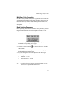
Image Analysis for Windows(r) v3.0 Software - License Agreement
BEFORE INSTALLING THIS SOFTWARE, YOU SHOULD CAREFULLY
READ THE FOLLOWING TERMS AND CONDITIONS. BY OPENING
THIS PACKAGE YOU AGREE TO BECOME BOUND BY THE TERMS
AND CONDITIONS OF THIS AGREEMENT, WHICH INCLUDES THE
SOFTWARE LICENSE AND LIMITED WARRANTY.
IF YOU DO NOT AGREE WITH THESE TERMS AND CONDITIONS, YOU
SHOULD PROMPTLY RETURN THE PACKAGE UNOPENED TO
MIRAIBIO, INC. (MIRAIBIO) OR A MIRAIBIO DEALER, AND YOUR
MONEY WILL BE REFUNDED.
The enclosed software (the "Software") is licensed, not sold, to you for use only
upon the terms of this Agreement, and MIRAIBIO and/or its licensor(s) reserves
any rights not expressly granted to you. You are responsible for the selection of
the Software to achieve your intended results, and for the installation, use and
results obtained from the Software. You own the media on which the Software is
originally or subsequently recorded or fixed, but MIRAIBIO and/or its
licensor(s) retains ownership of all copies of the Software itself.
LICENSE
You may:
a. Use the Software on a single machine at any given time.
b. In no manner engineer or reverse-engineer the copy protection hardware, or
whole or part of the software.
c. Copy the software only for backup or modification purposes, or to merge it
into other software, in support of your uses of the Software on the single
machine, provided that you reproduce all copyright and other proprietary notices
that are on the original copy of the Software provided to you. Certain Software,
however, may include mechanisms to limit or inhibit copying. Such Software is
marked "copy protected." Any portion of the Software merged into another
program will continue to be subject to the terms and conditions of this
Agreement.
d. Transfer the Software and all rights under this Agreement to another party
together with a copy of this Agreement if the other party agrees to accept the
terms and conditions of this Agreement. If you transfer the Software, you must
at the same time either transfer all copies whether in printed or machinereadable form, including all modifications and portions of the Software
contained in or merged into the other programs, to the same party or destroy and
copies not transferred.
RESTRICTIONS
You may not use, copy, modify, or transfer the Software, or any copy,
modification or merged portion, in whole or in part, except as expressly
provided for in this Agreement. Any attempt to transfer any of the rights, duties
or obligations hereunder except as expressly provided for in this Agreement is
void. YOU MAY NOT RENT, LEASE, LOAN, RESELL FOR PROFIT, OR
DISTRIBUTE.
TERM
This Agreement is effective until terminated. You may terminate it as any time
by destroying the Software together with all copies, modifications and merged
portions in any form. This Agreement will immediately and automatically
terminate without notice if you fail to comply with any term or condition of this
Agreement. You agree upon termination to promptly destroy the Software
together with all copies, modifications and merged portions in any form.
LIMITED WARRANTY
MIRAIBIO warrants for the period of ninety (90) days from the date of
delivery of the Software to you as evidenced by a copy of your receipt, or until
the Software is modified by you, whichever period is shorter, that:
(1) The Software, unless modified by you, will perform the function described in
the documentation provided by MIRAIBIO. Your sole remedy under the
warranty is that MIRAIBIO will undertake to correct within a reasonable period
of time any marked "Software Error" (failure of the Software to perform the
functions described in the documentation). MIRAIBIO does not warrant that the
Software will meet your requirements, that operation of the Software will be
uninterrupted or error-free, or that all Software Errors will be corrected.
(2) The media on which the Software is furnished will be free from defects in
materials and workmanship under normal use. MIRAIBIO will, at its option,
replace or refund the purchase price of the media at no charge to you, provided
you return the faulty media with proof of purchase to MIRAIBIO or an
authorized dealer. MIRAIBIO will have no responsibility to replace or refund
the purchase price of the media damaged by accident, abuse or misapplication.
THE ABOVE WARRANTIES ARE EXCLUSIVE AND IN LIEU OR ALL
OTHER WARRANTIES, WHETHER EXPRESS OR IMPLIED, INCLUDING
THE IMPLIED WARRANTIES OF MERCHANTABILITY AND FITNESS
FOR A PARTICULAR PURPOSE.
NO ORAL OR WRITTEN
INFORMATION OR ADVICE GIVEN BY MIRAIBIO, ITS EMPLOYEES,
DISTRIBUTORS, DEALERS OR AGENTS SHALL INCREASE THE SCOPE
OF THE ABOVE WARRANTIES OR CREATE ANY NEW WARRANTIES.
SOME STATES DO NOT ALLOW THE EXCLUSION OF IMPLIED
WARRANTIES, SO THE ABOVE EXCLUSION MAY NOT APPLY TO
YOU. IN THAT EVENT, ANY IMPLIED WARRANTIES ARE LIMITED IN
DURATION TO NINETY (90) DAYS FROM THE DATE OF DELIVERY OF
THE SOFTWARE. THIS WARANTY GIVES YOU SPECIFIC LEGAL
RIGHTS. YOU MAY HAVE OTHER RIGHTS, WHICH VARY FROM
STATE TO STATE.
LIMITATIONS OF REMEDIES
MIRAIBIO's entire liability to you and your exclusive remedy shall be the
replacement of the Software media or the refund of your purchase price as set
forth above. If MIRAIBIO or the MIRAIBIO dealer is unable to deliver
replacement media that is free of defects in materials and workmanship, you
may terminate this Agreement by returning the Software and your money will be
refunded.
REGARDLESS OF WHETHER ANY REMEDY SET FORTH HEREIN
FAILS OF ITS ESSENTIAL PURPOSE, IN NO EVENT WILL MIRAIBIO BE
LIABLE TO YOU FOR ANY DAMAGES, INCLUDING ANY LOST
PROFITS, LOST DATA OR OTHER INCIDENTAL OR CONSEQUENTIAL
DAMAGES ARISING OUT OF THE USE OR INABILITY TO USE THE
SOFTWARE OR ANY DATA SUPPLIED THEREWITH EVEN IF
MIRAIBIO OR AN AUTHORIZED MIRAIBIO DEALER HAS BEEN
ADVISED OF THE POSSIBLITY OF SUCH DAMAGES, OR FOR ANY
CLAIM BY ANY OTHER PARTY.
SOME STATES DO NOT ALLOW THE LIMITAION OR EXLUSION OR
LIBILITY FOR INCIDENTAL OR CONSEQUENTIAL DAMAGES SO THE
ABOVE LIMITAION OR EXCLUSION MAY NOT APPLY TO YOU.
GOVERNMENT LICENSEE
If you are acquiring the Software on behalf of any unit or agency of the United
States Government, the following provisions apply:
The Government acknowledges MIRAIBIO's representation that the Software
and its documentation were developed at private expense and no part of them is
in the public domain.
The Government acknowledges MIRAIBIO's representation that the Software
is "Restricted Computer Software" as that term is defined in Clause 52.227-19 of
the Federal Acquisition Regulations (FAR) and is "commercial Computer
Software" as that term is defined in Subpart 227. 401 of the Department of
Defense Federal Acquisition Regulations supplement (DFARS) The
Government agrees that:
(I) if the Software is supplied to the Department of Defense (DoD), the Software
is classified as "Commercial Computer Software" and the Government is
acquiring only "restricted rights" in the Software and its documentation will be
as defined in Clause 52. 277-19 (c) (2) of the FAR.
(II) if the Software is supplied to any unit or agency of the United States
Government other than DoD, the Government's rights in Software and its
documentation.
RESTRICTED RIGHTS LEGEND
Use, duplication, or disclosure by the Government is subject to restrictions as set
forth in subparagraph.
(c) (1) (11) of the rights in Technical Data and computer software clause of
DFARS 52.227-7013.
MiraiBio Inc.
1201 Harbor Bay Parkway, Suite 150
Alameda, CA 94502
EXPORT LAW ASSURANCES
You acknowledge and agree that the Software is subject to restrictions and
controls imposed by the United States Export Administration Act (the "Act")
and the regulations thereunder. You agree and certify that neither the Software
nor any direct product thereof is being or will be acquired, shipped, transferred
or reexported, directly or indirectly, into any country prohibited by the Act and
the regulations thereunder or will be used for any purpose prohibited by the
same.
GENERAL
This agreement will be governed by the laws of the State of California, except
for that body of law dealing with conflicts of law.
Future updates of the Software will be available for purchase by licensees for a
fee provided a registration card has been received by MIRAIBIO. Registered
Licensees will be notified of such updates as they become available.
Should you have any questions concerning this Agreement, you may contact
MIRAIBIO by writing to MiraiBio Inc., 1201 Harbor Bay Parkway, Suite 150,
Alameda, CA 94502.
You acknowledge that you have read this Agreement, understand it and agree
to be bound by its terms and conditions. You further agree that it si the
complete and exclusive statement of the agreement between us, which
supersedes any proposal or prior agreement, oral or written, and any other
communications between us in relation to the subject matter of this Agreement.
Addendum
Image Analysis v. 3.0
This document contains information regarding the latest changes made for the Image
Analysis v. 3.0.
1. LANE BENDING
When a handle point is clicked and dragged on a lane outline, the outline will swing in a
curved path making it easier for users to manually fit them on an irregularly shaped lane.
If the end points of the outline (i.e. top or bottom handle points) are clicked and dragged,
the corresponding portion (i.e. top or bottom portion) of the lane will bend like a fishing
pole being pulled. If any of the mid handle points are pulled, then the lane will bend from
that handle point resulting in a small arc.
When a control key is pressed while dragging handle points on a lane, then only a
particular segment (i.e. between two handle points) will be moved in a straight line and
not in a curved path.
2. POWER SCROLLING
For images bigger than the size of the window on the screen, any selection tool or
rectangle-shaped tool will cause the image to scroll to the end when the mouse cursor is
moved beyond the window border.
Suppose an image being analyzed is too big to fit in an application window and the user
has about 25 lanes for automatic lane detection. With this Power Scrolling feature,
selection tools and rectangle-shaped tools will cause the image to scroll as the mouse
cursor crosses the window border, until the user stops moving the mouse, or when the
image cannot be scrolled any further.
As of now, the following tools now have this new feature:
Ellipse tool on Draw Toolbar
Rect Tool on Draw Toolbar and Create Rect Angle Spot tool in Medium Grid Toolbar
Oval Tool on Draw Toolbar and Create Oval Angle Spot in Medium Grid Toolbar
Text Tool on Draw Toolbar
Select Tool on Draw or 1D Tool Toolbar or Medium Grid Toolbar
Lane Selection Tool on 1D Tool Toolbar
Multiple Lane Selection Tool on 1D Tool Toolbar
1
3. MAGNIFICATION
Magnification Range has been extended
up to 3200 %. This new feature allows
end-user to magnify the image that is
scanned with high resolution of 25 µm.
In addition, images with 72 Dpi Screen
Resolution can be loaded without
resulting in an error.
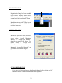
4. OD CALCULATION
In 1D-Gel->Preference dialog box, there
is an extra box where end-users can
select either “Overall Maximum
Intensity” or “Average Pixel Intensity”
algorithm to calculate OD values. The
default setting is Average Pixel
Intensity.
In general, “Average Pixel Intensity” can
give better result for most images.
5. COLOR SEPARATION
Users must set background noise value for each channel before clicking on “Set”
button to calculate Channel-Parameters for color separation.
2
To select a background for a particular channel, locate a band that is known
to be in that channel. Then select an area that is blank next to that band and
then click “Set” button. User must do this for each and every channel before
setting each color separation parameters.
Also, while in Image->Color Separation dialog box, users CANNOT assign or
change any channel’s color. The color assignment has to be changed in “Image
Settings” dialog box before bringing up “Color Separation” dialog.
6. FOUR CHANNEL SUPPORT
To have four channels support to function properly, the image must be in
“OVER” mode or “MONO” mode.
3
"
#
&
'
#
$% &
$$
#()%$
$
#
*
,
-
$ #()%$
$.#
#()%$ $
#
#
,
-
#()%$ $.
#()%$
'
#%#
!
!
!
!+
!+
!+
!
!
!
!
!/
&%#
+!
+!
+!+
+!
.
-
$-
1 $
1
(
$#()%$
$!
2
+!0
+!0
+!
+!/
'%#
!+
!
)
3
1
-
% #
$
% -
*
$$ $
,
$ $
)$
$
$
$*
*
% #
$
$
#
12
$$-$1
$
$
$ #
$-
(
$
$*,7
1%
$#()%(
!
!0
!
!4
!4
!5
!5
!
!+
!+
!+
!
)%#
0!+
0!
0!0
0!
0!/
0!6
0!4
0!4
0!4
0!4
0!5
0!
0!
0!
0!+
0!
0!
+
$-
$-
.$-
1$
-
#
#(
-
(
#()%(
)
(!-
,
#
3' $
3
-
7
-2
7
% 7
$
7
(8
$
9(!-
$1
)
'
1 (
1 -
---
-,
1 1)
*,7
0!0
0!
0!/
0!6
0!4
0!4
0!+
0!+
0!+
0!++
0!+
0!+
0!+
0!+6
0!+
+%#
!
!
!
!
!0
!6
!5
!
!
!
!
!+
!+
!
*$7% *,7
1
*
$ $
(
$,(
-
$ -
$ 8
)-
$ .-
$ 8 (
-
$ 8 ):
1!*(8
(!)-
$ )$
(!)-
$ ,
1,
1 ,,
3,)
-
1,
$( ,
,8 1(
1)
)1
() $(:
(:
!
!/
!+
!+0
!+
!+
!+6
!+5
!+5
!
!0
!0
!
!6
!0
!0
!00
!
!
!
!
!0
!0
!
!4
!/
!/
!/0
!/4
!/4
,
.
3' (:
!6
:(:8 !6+
(:8 !6+
)$-
!6
-9
:;
!66
):
9
!64
-2
<9
=%1> !64
9
-
8 !64
$?
(:
!65
9
-
!4
1 !4
. $ 9
!4
3' $ !4/
%8
!46
%8
!46
%8$
!5
3' ,81
!5
!50
)
!5/
!5/
#-%
,%#
1!*(8
/!+
<1!*
/!/
$
$ /!/
$!-
3' #
/!6
$!-
3' /!4
(!-
3' #
/!/
(!-
3' /!6
.%#
(8
6!+
/
0
-
<$ -*
(
*
*
$ *
-8 ):
-
):
9
(:
$?
(
-
1 $ 3' $ -
*
1$#
%9#
*-
#
$
#
-
1(8
!:(
$(
8'
18
:1%7
-
$
,;
8
6!
6!
6!/
6!5
6!5
6!
6!
6!+
6!
6!/
6!4
6!4
6!+
6!+
6!++
6!+
6!+4
6!
/%#
4!+
4!
4!
4!0
4!6
4!0
0%#
5!
5!
5!+
5!+
#1
% 8 5!+
(
$.
5!+
$ 5!+
$
5!
8
$.
5!
3
,#
5!
5!
$ $.
5!
#
%7$.
5!0
3@ -
1 5!0
.:
-
1
5!0
"
(* "
#1%#
$8 -$
!+
$8 -
!
9
!+
@
!+
$8 -
!+
$$8 -
!
$8 -
!
$8 -
!(
9
!
@
!
$8 -
!0
$$8 -
!
$8 -
!
$
8 !/
3
!6
3' 1!*
!4
.$8 -
3
!5
% !
$8,
: 8
!
$8
!0
$8
-
$
3' 1
-%1$
%
*
"
$
!8
#38
8
1!*8
(!)-
$ 8
8%8
8
18
8
'
!+
!+
!+
!+
!+
%#
!
!+
!+
!
!/
!5
!
!
!
!
2!
!$
(3
( 3
456*
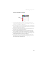
For your safety, operate this equipment only as prescribed by the instructions
in this manual. Operation outside these parameters may subject the purchaser to waive any liabilities by Hitachi Software Engineering Co., Ltd.
In addition, any claims deemed to arise due to failure to thoroughly read this
manual may result in the waiver of any liabilities by Hitachi Software Engineering Co., Ltd.
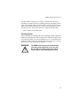
The following symbols are related to safety concerns. Please ensure that you
understand the meaning and implications of each symbol before continuing
to read this manual.
7*889
!
"89
!
(
(
:
(;
(
(((
(<
8
7
@ @ (
Each symbol indicates the type of warning illustrated.
Cautions the user of a particular hazard (in this case, of potential
electrical shock).
This symbol represents prohibited actions.
0
7*889
!4
!
-8
-*
Please do not disassemble or attempt repairs. Tampering with the
internal components risks exposure to such hazards as electrical
shock and laser radiation.
(
(
7
Shield the Scanning Unit from water. Never place objects containing water or other fluids on the Scanning Unit. A spill can lead
to short circuits or electric shock. If there is a spill, immediately
turn the power switch off, disconnect the power cord and contact
your nearest authorized Hitachi Software Engineering Service
representative.
8:
Keep foreign objects out of the Scanning Unit. Do not allow paper
clips, hairpins, metallic objects, paper or other combustible
material to fall in or otherwise enter the Scanning Unit. Foreign
objects in the Scanning Unit can lead to short circuit, fire or
electric shock. If this should happen, turn the power switch OFF,
disconnect the power cord and contact your nearest authorized
Hitachi Software Engineering service representative.
0
7*889
4
(
!
!
(!"
Ground the Scanning Unit with the proper power cord with the
three-prong plug provided with the Scanning Unit. Before
turning on the Scanning Unit, check that the power cord is NOT
damaged. Using the damaged power cord can lead to short circuits, fire or electric shock. If the power cord is damaged, turn
the power switch OFF, disconnect the power cord and contact
your nearest authorized Hitachi Software Engineering Service
representative for a replacement. Use only a properly grounded
three-prong power cord as a temporary replacement.
-8
8%
!
Use the specified power supply (AC100 V and 50/60 Hz). Use
only with the proper voltage and frequency indicated on the
specification plate on the rear of the equipment. Use of other
than the proper power specifications may lead to accidents and
equipment malfunction.
0
#
$$
$
(=
Thank you for purchasing Hitachi Software Engineering Company, Limited,
FMBIO scanning unit, a device for reading the electrophoresis patterns of
fluorescent dye-marked samples. FMBIO represents a maturing of fluorescent technology that has been applied to life sciences labs since the
1960’s. Some of the major benefits associated with the system are improved
safety, speed, accuracy, and lower cost.
Read this manual carefully before attempting to operate the system and carefully heed all safety warnings.
$
The FMBIO system eliminates the risks to lab personnel, the need for radioactive shielding and the storage and procurement problems associated with
handling I125, C14, S35, and P32.
*
With the FMBIO, speed of experimental throughput is substantially greater
because scanning and analysis are independent of electrophoresis. Many
more gels can be run and scanned with the FMBIO than with a dedicated
electrophoretic sequencer.
The FMBIO reads gels, membranes, and plates without the need for x-ray
film or costly phosphor screens. Over- and under-exposure problems are
eliminated. Scan times for the FMBIO are typically five to ninety minutes,
considerably less than the eight hours development time required for conventional radiography. FMBIO images are processed without removing glass
plates, drying gels, or developing film, saving more time. Using multi-wavelength scanning, samples labeled by two or more different fluorophores can
be read in one scan.
1-1
Accuracy, sensitivity, and flexibility of experimental operations are
improved with the FMBIO system. 16 bit imaging allows detection of signal
intensity over a much greater linear dynamic range than isotope-based
systems. This enables both dark and light bands to be read in the same experiment. Many of the errors that stem from sample handling are virtually
eliminated because glass plates are not removed, gels are not dried, and readability of results does not depend on exposure time. Because scanning does
not require removing the gel from the glass plate, gels can be run, then
scanned, then run and scanned again, increasing the number of readable
bands per gel.
6"
When the FMBIO system is in place, the expense associated with X-ray
film, storage phosphor screens, shields, badges, Geiger counters, low temperature freezers, and disposal services is eliminated.
The FMBIO consists of a scanning unit and two software applications that
run on Microsoft Windows 95 or 98. The Read Image scanning software
controls the operation of the scanner, and the Image Analysis software
carries out the analysis of the scans. The two software applications may be
run on separate computers if desired.
D*
=
The FMBIO scanning unit detects laser-induced fluorescent signals on gels,
blots and thin layer chromatograms. It accommodates plate sizes up to 600 x
400 mm, with a maximum reading size of 550 x 400 mm. The excitation
sources are two or three solid state laser.
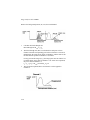
The laser's sample unit moves across the optical unit (Y direction) as its laser
beam is directed onto the sample (X direction) via a polygon mirror rotating
at high speed. The resulting fluorescent light signals emitted from the
excited fluorophores are then collected by two optical fiber arrays.
The instrument also features two photomultiplier tubes, a large scan area of
55x40 cm, and a linear dynamic range of four orders of magnitude. The
FMBIO produces extremely high resolution images capable of resolving
even single-base microvariants.
Fluorescent probes that are responsive to the frequency of the laser beam
emit fluorescent signals upon being excited. The emitted light is collected by
a lens and directed into a fiber optic array which passes it to an interference
filter. The targeted fluorescence wavelength passes through the interference
filter and then to a photomultiplier where the light signal is converted to a
digital signal. Conversion of the digital signal to experimental data takes
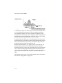
place in the data acquisition circuits, where fluorescence detected at the photomultiplier is synchronized with the angle of rotation of the scanner mirror
and with the horizontal motion of the sample unit to produce positional
values in the sample. See Figure 1-1.
D<
.
,
,
#
% #%#<
$=
Multicolor imaging is achieved using band-pass detection filters to discriminate light from fluorescent dyes emitting between 300 and 700 nm. Up to
four filters can be stored in the instrument and accessed through software.
Two filters can be used simultaneously to detect emissions from two different dyes.
In multicolor analyses, the gel is scanned after electrophoresis using optimal wavelength
band-pass filter to detect various flurorescent dye-labeled products.
These images can be overlaid into a multicolor image or viewed separately.
The maximum number of overlay is 4-color.
D@
=
80 :
%
46=>'/=1>'=;>
% 5!A-
% +!4B
,'
635nm, +, 488nm (optional)
3
$&3!6
1
= >
&
C
#
&+
C
<='>
600 =>' 400 =1>'=;>
$='>
550'400
1
=>
. 25D' E
/=//>
, 10FG
H*
@
C/;<
F
CCC+C++C+09
=->
Ensure that the voltage and frequency of the power source correspond to
FMBIO power settings. Check the power settings on the specification panel
on the rear of the machine. Verify that the building power supply has a functional ground.
The FMBIO software consists of two modules: FMBIO Read Image and
Image Analysis. These applications function independently and need not be
installed on the same computer.
D
This application controls the FMBIO scanning
hardware, synchronizes the fluorescent input signal with the scanning mirror
and optical unit, and converts this data into a bitstream. Read Image is used
to easily set the scan area, scan resolution, image orientation, and photomultiplier sensitivity. The user can also choose filters, add comments to be saved
with the scanned image, and perform hardware checks. The experimental
data collected are converted by Read Image into a 16 bit digital TIFF file for
analysis with the Image Analysis software. The scanning software provides
a 16 bit gray scale image of fluorescence intensity, with a broader linear
dynamic range than possible with conventional autoradiography.
This application offers a user-friendly interface for
viewing and analyzing images. The software features analysis functions that
include automatic band detection to facilitate data processing, quantitation
of peak height or peak area, and band sizing through comparison to size
standards.
With fluorescent dyes for sample labeling, and the FMBIO software the
system can analyze:
E
E
E
FA"*"B
9A
571B
D
D$$
Multi-wavelength analysis makes it possible to create and analyze multicolor signal images. You can run fluorophores of multiple spectra in the
same lanes, and simultaneously scan their emission signals. This function is
useful for comparative allele analysis or, when a marker of known size is
added to the lane, for highly accurate size determination.
FMBIO software contains spatial analysis functions that accurately estimate
fragment migration distances. It also contains signal intensity analysis functions, so that it can perform densitometry to estimate band or spot intensity.
6
With the FMBIO, you can select from a wide range of fluorophores, from
rhodamine red to fluorescein green and including tetramethylrhodamine, Xrhodamine, beta-phycoerythrin, ethidium bromide, propidium iodide.
Because of the powerful intensity of the FMBIO laser, you can use fluorophores with emission wavelengths closer to the excitation wavelength.
D'
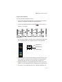
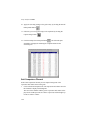
Table 1-2 shows a list of dyes and stains that can be used with the FMBIO,
along with recommended filters.
Almost all molecular species absorb and then re-emit light under certain
conditions, giving a broad emission spectrum, up to 100 nm wide in condensed media. When the emission process (the excited state) takes place at
the nanosecond or a slower time scale, the phenomenon is called
fluorescence.
D?
#%&2Selected -
-
(
(=
-
>?
>?
@
>?
A
$ %
06+
6
4
(
$ /+
/+
(
3)
/
$*
05
+
(
;$
+
/
/
(
#8-#
05
+
#(
05
:!3
I%3
+/
04
4
:!3
;3J
+5
/
4
:!3
8(
5
64
4
:!3
8
0/
6+
J
60
5
/
(
8'
64
/+
/
(
%J
4
/
/
:!3
)
/
/+
/
(
%%
+6G5
/6
4
(
)%%
+6G6
/
/
(
)%)%
+0G6+
/+
/
(
4C/ (
K.
'
D(
-
>?
>?
@
>?
A
-+
045
-
+
/
4
-
4
5/
/
#
J
050
+
0!00
/
I),
/
9
,
9
K.
'
D>
& !
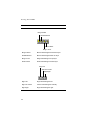
7*889
!
((
(;
<*$
(
("
(
(<
"
=(
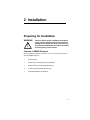
Before beginning installation, check that you received the following items
with the FMBIO shipment.
$.
(2 m long) and two-prong adapter
Blower brush (for cleaning optical devices)
2
Fuses (3A) (stored inside the AC inlet)
% s (605nm and 505nm)
2-1
Installation-FMBIO
(
Instrument and software installations are performed by qualified Hitachi
Service personnel. Any unauthorized attempt to install the scanning unit
could void the instrument warranty.
Prepare a level, sturdy, non-vibrating surface in a well-ventilated,
temperature-stable area for the FMBIO scanning unit. The unit should not be
placed in a dusty or damp location, or in an area where it will be subject to
vibration or impact. Allow at least 10 cm of clearance next to the rear and
left panels. Do not place heavy objects on top of the scanning unit. Keep the
scanning unit away from flammable or corrosive gases.
2
2-2
8s
#()%@
!
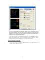
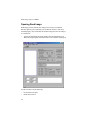
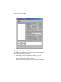
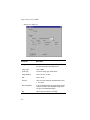
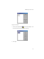
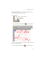
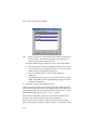
G FMBIO-Installation
(=
FMBIO system requirements:
•
IBM® or 100% IBM®-compatible personal computer
•
Windows 2000
•
Pentium II 300 MHz or greater is recommended
•
128 MB RAM minimum (256 MB or more recommended)
•
10 MB free (minimum) of hard disk storage space is required for
program loading. Image and spreadsheet files could require substantially
more storage space
•
CD-ROM disc drive is required for
installation
•
Resolution: 1024 x 768 or higher, 16 bit color display or higher
•
Mouse or other pointing device
•
Keyboard
The FMBIO software can be obtained on a CD.
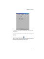
To install the FMBIO software contained on a CD:
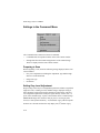
1.
Turn off the screensaver.
•
In the Windows Taskbar, click on the Start button. Choose Settings
> Control Panel.
•
Double-click the Display icon.
•
Click the Screensaver tab, then select None.
2.
Disable all virus protection programs.
3.
On the CD, open the ReadMe file to find out about changes and updates.
4.
Click the Start button, then choose Run....
5.
Enter the pathname for the setup.exe file on the CD (for example,
D:\setup.exe), then click OK.
6.
Follow the instructions on the screen.
2-3
Installation-FMBIO
!"
Users of the FMBIO system should be familiar with basic IBM-compatible
computer and Windows 2000 functions. New users should familiarize
themselves with Windows 2000 operation before attempting to operate the
FMBIO system. Refer to your manuals and the online help installed with
Windows 2000.
"-
1.
In the Windows Taskbar, click on the Start button. Choose Settings >
Control Panel.
2.
In the Control Panel window, double-click the Display icon.
3.
Click the Settings tab, then select the 256 Colors setting or higher.
2-4
FMBIO-Installation
Note
When 256 colors are selected, only the active window is displayed
with sharpness and clarity, while background windows may have a
rough appearance. When High Color (16 bit) or True Color (32 bit)
is selected, all windows are displayed with sharpness and clarity,
but at the cost of slower screen drawing. The number of colors you
choose depends on the complexity of your images and the speed of
your system.
!
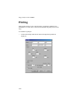
Images generated by the FMBIO system can be printed on conventional
postscript laser printers with 600 dpi resolution. While the images rendered
by such machines are adequate for many reference and record-keeping
purposes, much information is necessarily left out of images printed on such
machines. Always remember that images printed on such machines are
schematics that do not faithfully represent all the information available in the
digital image in the FMBIO file.
2-5
Installation-FMBIO
High quality images that more faithfully represent in hard copy the
information present in the FMBIO image file can be created using a high
quality image printer. Image printer capability should include 256 grayscale,
3-color dye sublimation, and 300 dpi or higher.
!(
-$
A single digital image file may be 10 MB or larger. To conserve hard drive
space, you may store files on a peripheral storage device.
2-6
'
(
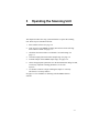
This chapter describes the steps you should follow to operate the scanning
unit. These steps are summarized below:
1.
Start Scanner software. See page 3-2.
2.
Turn on power to the FMBIO scanning unit and wait for the self-diagnosis routine to finish. See page 3-2.
3.
Check that the 605 nm filter is in Channel 1 for autofocusing. See
page 3-5.
4.
Clean the sample plates and scanner sample stage. See page 3-8.
5.
Load the sample on the FMBIO sample stage. See page 3-10.
6.
Choose the appropriate parameter set in the Scan Parameter dialog box and,
if necessary, adjust the scanning parameters. See Scanner
Software.
7.
Use Scanner software to begin scanning the sample. A scan may
take from five to ninety minutes.
See page 3-13 for Guidelines to Scanning with the FMBIO Scanner
software.
3-1
Operating the Scanning Unit-FMBIO
(=
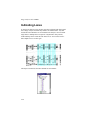
Turning on the power to the scanning unit first, then turn on the computer and
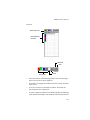
start the FMBIO Scanner software.
•
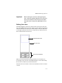
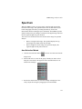
To start the Scanner program, double-click the Scanner icon.
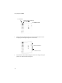
The FMBIO scanning unit has two electrical switches:
•
The Main switch, located on the rear panel next to the SCSI
cable port
•
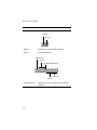
A Power switch, located inside the front panel
For both electrical switches, the Off position is marked with a circle () and
the On position is marked with a vertical line ( B ). The locations of the power
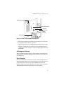
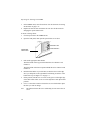
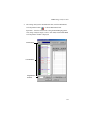
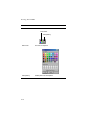
switches are shown in the following two figures.
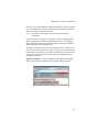
G
3
'%#<
(!
(
3-2
FMBIO-Operating the Scanning Unit
$-$ ( - G
$-$
'%&<*$=
1.
Turn on the computer that is connected to the scanner by a SCSI cable.
2.
Set the Main switch to the On ( | ) position.
3.
Open the front panel of the scanning unit and turn on the Power switch.
When the scanning unit is first turned on, it automatically performs a
self-diagnostic routine. During the routine, the Ready light on the front
panel blinks.
%8
When the Ready light shines steadily, without blinking, the self-diagnostic
routine has been completed without detecting a problem. You may now use
the scanning unit.
-
When the self-diagnostic routine detects an error, the Ready light shuts off
and the Error light begins to glow. Turn off the Power switch for at least five
seconds, then turn on the Power switch. The FMBIO repeats the selfdiagnostic routine. If the routine detects an error again, contact your nearest
authorized Hitachi Software Engineering service representative.
3-3
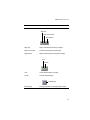
Operating the Scanning Unit-FMBIO
"89
!
7*889
!
$ #()%<;
7
7
8=
+1%7%
<
%
$<
%
((
(
<
C
C
C
7*889
!
-
$
(
<
-
(
<
-
$
(
$
(=
<
(5
(($
(5(
3$
$
<
4
(
$<
"
After a power-up, the FMBIO automatically performs an autofocus before
beginning the first scan. Channel 1 does not have to be active during an
autofocus, but it must contain the 605 nm filter.
After the initial autofocus, you may remove the 605 nm filter and replace it
with a filter that accommodates a detection range compatible with the stain
or dye you are using on your sample.
3-4
FMBIO-Operating the Scanning Unit
"89
$
.
#
G
!
Prepare for a scan by placing the appropriate filters in each channel. Only
active channels collect image data during the scan. See Selecting Active
Channels on page 4-14 for information about active channels.
The FMBIO scanning unit can accommodate two filter holders. Each filter
holder can hold two filters. You must place the appropriate filters in the
scanning unit before beginning a scan. Once the scan begins, the optical unit
moves out of home position and the filters are no longer accessible.
Note
If this is the first scan after turning on power to the FMBIO unit,
insert the 605 nm filter in the Channel 1 position.
If the automatic initial autofocus has been completed, turn off Auto
Focus in the FMBIO menu, and replace the 605 nm filter with a
filter appropriate to your scanning needs.
2
#()%G
G
:
H
$8 !+
!4
1.
To stop the scan, click the Pause button.
2.
A dialog box opens to display three options: Save, Don’t Save, and
Cancel:
•
To stop scanning, return the optical unit to home position and save
the scan data, click Save. Continue to step 3.
•
To stop scanning and discard the scan data, click Don’t Save and
continue to step 3.
•
To continue scanning, click Cancel to close the dialog box, then
click Resume.
3-5
Operating the Scanning Unit-FMBIO
3.
In the FMBIO menu, turn off Autofocus. See the directions for setting
an autofocus on page 4-13.
4.
Replace the 605 nm filter and restart the scan. See the directions for
changing the optical filters below.
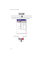
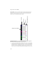
To insert or change filters:
1.
Choose Eject Filter in the FMBIO menu.
2.
Open the front panel, then open the optical filter service door.
-L
% 3.
-+L0
Pull out the appropriate filter holder.
The filter holder in the top position holds filters for Channel 1 and
Channel 3.
The filter holder in the bottom position holds filters for Channel 2 and
Channel 4.
4.
Hold the filter holder in your left hand, so that the arrow on the edge
faces you and points to the right and the ball bearing on surface of the
holder faces up. See Figure 3-3 on page 3-7.
5.
In this position, find the two set screws in the groove on the right edge
of the filter holder. There is one set screw adjacent to each optical filter
position.
6.
Use a 1.5 mm Allen wrench to loosen the set screw that holds in place
the filter you want to change.
Note
3-6
One full turn loosens the screw sufficiently; do not remove the set
screw.
FMBIO-Operating the Scanning Unit
$
# )
#
'%'<"(
7.
After one full turn of the set screw, hold the filter holder over a clean,
lint-free tissue and gently tilt the holder upright until the filter falls out.
Set the filter aside.
8.
Return the filter holder to a horizontal position and hold the replacement
filter over the appropriate hole in the filter holder. The alphanumerics on
the edge of each filter should be upright. If there is an arrow on the edge
of the filter, it should point up. Drop the filter in place.
9.
Turn the set screw one full turn to tighten the filter.
2
8
:G
10. Return the filter holder to its place in the scanning unit. Be sure the
finger hole in the filter holder is nearest to the service door. Close the
optical filter service door.
3-7
Operating the Scanning Unit-FMBIO
!
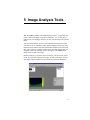
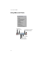
You can use the FMBIO system to scan and generate an image of:
•
Gels —1D and 2D
•
Membranes —Southern, Northern, Western, dot, slot, and TLC
•
Low- and medium-density arrays
("$
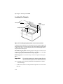
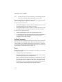
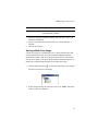
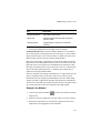
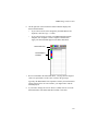
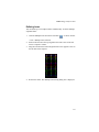
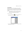
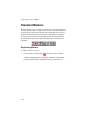
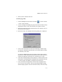
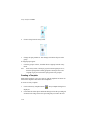
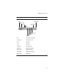
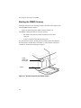
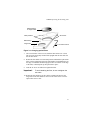
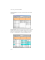
Below is a figure that shows the location of the button which, when pressed,
causes the top cover to open.
'%)<
$=
When the cover is open, you can access the glass plates and the scanner
sample stage.
3-8
FMBIO-Operating the Scanning Unit
2
G
G
!
The scanning unit accommodates a glass plate that is 400 mm wide x 600
mm long and 5.0 mm thick ± 0.1 mm. For best results, only use lowfluorescence borosilicate glass of “Tempax” or similar grade. The use of
other grades or sizes of glass may result in poor scanning quality.
The sample stage supports the sample plates on two sides only to allow the
maximum area to be scanned, and when the glass plate is properly seated on
the scanner bed, the scannable area is 400 mm (width) x 550 mm (length).
Be careful when loading the sample stage; use both hands, lower the sample
plate gently onto the stage supports, and close the scanning cover gently.
Sample plates break easily, and broken glass inside the instrument exposes
the operator to cuts and the equipment to mechanical damage.
Fingerprints, reagents and other foreign objects on the glass plate surface can
cause noise in the image and may even show up as a signal.
•
Keep the surfaces of the plates clean. Use soap and water, plain water, or
70% methanol (MeOH) to clean plates. Avoid using ammonia-based
glass cleaners. Wipe plates until dry to avoid streaks.
Dust and particles on the sample stage reflect stray light which can increase
background signal or cause loss of signal.
•
Keep the sample stage clean, particularly the autofocus strip and adjacent areas.
•
Regularly use the cleaning mode to clean the mirror and lens that passes
below the sample.
•
Wipe the stage and interior areas with a damp, low-lint cloth.
•
Immediately wipe off any gel or samples that fall onto the sample supports or into the unit itself.
3-9
Operating the Scanning Unit-FMBIO
6
(
* $
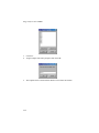
$ '%+<6
(
(
To maximize the scannable area on the glass plates, the scanner supports the
sample plate only on two ends. Take great care when placing the glass plates
on the scanner bed to avoid breaking the glass plate and damaging both the
sample and the scanning unit.
Orientation of glass plates. Scanning begins in the upper left corner of the
scanner bed, near the sample alignment surface. (See Figure 3-5.) The longer
of the two glass plates should rest on the sample supports.
Removing spacers. It is not necessary to remove the spacers on the glass
plates.
2
#
<<G
Note Begin the scan as soon as possible after electrophoresis to ensure a
clear scan image.
1.
Set the Power switch to the On position and open the cover of the scanning unit.
3-10
FMBIO-Operating the Scanning Unit
2.
Clean and thoroughly dry the surfaces of the glass plates. You may want
to mark the front of the plate so that it can be distinguished on the scan.
3.
Before putting the glass plate on the scanner bed, adjust the sliding
sample support so that it is ready to accommodate the length of the plate.
4.
Carefully and firmly place the end of the longer glass plate up against
the sample alignment surface. See Figure 3-5 on page 3-10.
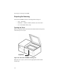
5.
As you carefully begin to lower the rear end of the glass plate to lay flat
on the scanner bed, finely adjust the position of the sliding sample plate
so that it offers full support.
6.
When both ends of the glass plate are firmly supported on the scanner
bed, gently close the scanning unit cover to avoid vibrations that might
unsettle the glass plate. You can hear a clicking sound when the cover
shuts.
7*889
!
6
(
(
($
(
<
%
$
(%
<"( (
(
$
(
<
3-11
Operating the Scanning Unit-FMBIO
(
The sensitivity of the scanning unit is dependent on a number of factors
including: the dyes or stains used; the quality of the reagents; gel density and
the diffusion rate of the sample in the gel; protocols and technique. You can
fine-tune the image scan by adjusting the scanning parameters in the Read
Image dialog box.
Before beginning a scan, read Chapter 4, Scanner Software, to become
familiar with the features of this software.
=
(
Once you are satisfied with the Scanner software scanning parameters, click the
Read button on the Read Image dialog box to begin the scan.
Auto Focus. After the Power switch is first turned on, the FMBIO Read
Image software automatically performs an autofocus before it begins the
first scan. During autofocusing, the rotating mirror and other signal tracking
and processing elements are adjusted to optimize optical alignment. The
entire process requires about thirty seconds to complete. The 605 nm optical
filter should be in Channel 1 during autofocusing.
After the initial autofocus, you can turn autofocusing off and on with Read
Image software. See page 4-13 for more information.
After the initial autofocus routine, you may stop the scan and replace the
605 nm filter with a filter of a different wavelength. See Autofocus
Calibration on page 3-4 for more information.
When you stop a scan in progress, you either save or delete the partially
scanned image.
1.
To stop a scan in progress, click Pause.
2.
A dialog box offers three actions after you click Pause: Save, Don’t
Save, and Cancel:
•
Click Save to save scan data and end the scanning process.
•
Click Don’t Save to discard scan data and end the scanning process.
•
Click Cancel to close the dialog box, then click Resume to continue
3-12
FMBIO-Operating the Scanning Unit
the scanning process.
Following is a list of guidelines for use when scanning with FMBIO Read
Image.
Auto Focus. After the FMBIO is turned on, it performs an autofocus before
it begins the first scan. The 605 nm filter must be in Channel 1 position
although Channel 1 does not have to be active during the autofocus.
PreRead. Use PreRead to identify the area of interest on the sample and to
make sure that spacers and other reflective items are not included in the scan
area.
Scan area. The rectangle on the Scan Control window represents the total
possible scan area. You may specify a smaller rectangle within the total scan
area to represent a pre-defined scan area. By default, Read Image displays
the last scan area used with each Parameter Set.
Time. The amount of time it takes to perform a scan is a product of the area
of the scan, the resolution (dpi), and the number of repeats per scan line.
Repeats. As you increase the number of repeats per scan line, the signal to
noise (background) ratio increases.
Signal. At lower resolutions, the amount of visible signal may increase, but
resolution of bands and spots decreases.
Resolution. The resolution of bands and spots improves as you increase
both resolution (dpi) and repeats per line.
Saving parameters. You can save a set of customized scanning parameters
as a Read Image file. You can open this file and reapply the saved settings to
new scans.
Multiple scans of the same gel. If necessary, you can remove a gel from the
FMBIO scanning unit, remount it in the gel box for additional
electrophoresis, and then rescan the gel.
3-13
) *
The Read Image software controls the FMBIO scanning unit as it generates
digital images of gels, membranes, blots, and microtiter plates. Read Image
converts the experimental data into a digital file which you can store on the
computer hard disk or on a peripheral storage device. You can then use
Image Analysis software to analyze the image.
Note
This manual does not discuss sample preparation. Refer to standard
texts such as Ausubel or Maniatis, and to the documentation accompanying your fluorophores.
With Read Image software you can:
•
Define the type of material being scanned and the scan area
•
Set scan resolution (dpi) and number of repeats
•
Adjust PMT sensitivity
•
Adjust cutoff thresholds for background and signal
•
Adjust the focusing point
•
Set and save an autofocus routine
•
Add comments to be recorded and saved with the scanned image
•
Create and save customized scanning preferences
The procedures discussed in this chapter can be used with all types of scannable materials.
An example which illustrates some of the procedures begins on page 4-27. It
is followed by a troubleshooting guide on page 4-31 and a list of error codes
on page 4-32.
4-1
Read Image Software-FMBIO
*
Read Image provides default scan settings for four types of scannable
material: agarose gels, acrylamide gels, membranes, and TLC (thin layer
chromatography). You can modify the default settings and save the changes
as a custom file.
•
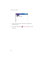
To start the Read Image program, double-click the Read Image icon.
When the program opens, an untitled Scan Control window is displayed.
Use this window to do the following:
•
Pre-read the scan object
•
Define the scan area
4-2
FMBIO-Read Image Software
•
Read the scan object
•
Provide a unique name for the image
•
Enter comments
For more information about this window, see page 4-15.
*
You can save all the Read Image parameters in a file. When you open a saved
Read Image file, the Scan Control window is displayed. Read Image automatically displays the scanning parameters. You may modify these
parameters or apply them unchanged to a new scan.
•
Use the commands in the File menu to create, open, and save Read
Image files. See page 4-20 for a description of this menu.
4-3
Read Image Software-FMBIO
(!
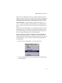
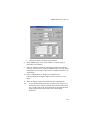
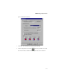
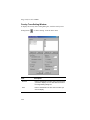
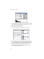
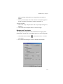
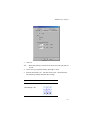
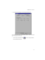
To set the FMBIO parameters, choose Set Parameters... in the Command
menu.
Use the Setting dialog box to specify:
•
Parameter name
•
Scanning resolution
•
SCSI ID
•
Experiment type
•
Channel name, sensitivity, and filter
•
Focusing height
•
Scan line repeats
For more information about this window, see page 4-6.
4-4
FMBIO-Read Image Software
!
Use items in the Command menu to specify:
•
Gray level adjustment settings, including high and low cutoff thresholds
•
Orientation of the scanned image
See page 4-10 for more information about this menu.
Use items in the FMBIO menu to choose:
•
Autofocus
•
Active channels
See page 4-13 for more information about this menu.
4-5
Read Image Software-FMBIO
(!
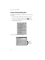
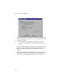
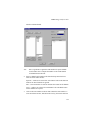
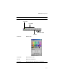
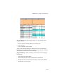
7
8
4-6
-
2
;
<
$-$1
$-$1
#()%
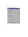
3' 8 .
' -2
.
$
(8
#
#
#
#
=&!+
M >
2
FMBIO-Read Image Software
The most appropriate parameter values for your experiment depend on image
quality (signal to noise ratio), sample volume (heavy bands or faint bands),
and fluorophore chemistry. Improper scan parameters may lead to images
saturated with signal or images so faint that missing important elements,
such as weak bands, are missing. If in doubt, it may be helpful to scan a
portion of the image a number of times using different parameters, then
choosing one set of parameters for the entire image.
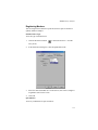
1.
In the Parameter Name pull-down list, choose the material type you
want to scan.
Each parameter name is associated with default settings for the scanning
parameters.
2.
Examine the parameters in the window and modify them as needed to
accommodate your particular experimental conditions.
3.
Click OK to apply the scanning parameters to your scan. See page 4-15
for information about defining scan area.
-
(!
8
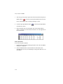
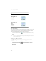
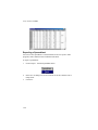
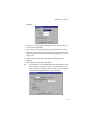
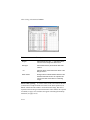
The Parameter Name list contains various types of scannable material. Five
parameter names are available: agarose gel, acrylamide gel, membrane, and
TLC (thin layer chromatography). Each parameter name is linked to a predefined set of default scanning parameters.
6"
;
< 9 +/
+/
+/
+/
-
4
4
0
0
+-
-
4
4
0
0
0-
You can modify any of these parameters as needed to accommodate your
particular gel conditions. You may also specify and save a customized set of
parameters for repeated use. See page 4-20.
4-7
Read Image Software-FMBIO
"The SCSI ID of the FMBIO scanning unit is set to 6 at the factory. If you
have any other peripherals attached to the SCSI port of the computer, make
sure they do not share the same SCSI ID number.
•
Verify that the SCSI ID is set to Auto or 6 in the Read Image software.
(**
The higher the resolution, or dots per inch, of the scanned image, the more
information is collected during the scan. The resulting file for a scan collected at a higher resolution requires more storage space. You can specify
resolution for both vertical and horizontal scan directions. Each parameter
name has a limited number of resolution choices for each direction.
•
Select horizontal and vertical scan resolutions.
*
$
The intensity of the charging voltage generated by the photomultiplier tube
(PMT) influences how much of the collected light signal is considered as
viable data. The higher the voltage, the greater the sensitivity and the more
background signal is included in the data. Material with inherent high background signal, such as membranes, require lower reading sensitivity.
When you use more than one filter to produce an image, one or more fluorescent signals may be noticeably stronger than the others. You can adjust
the sensitivity of each channel to equalize the intensity of the signals.
2
•
H
#()%
$ 0!
Enter a value between 0-100% for each channel. Read Image
automatically assigns a value of 0% to sensitivity fields that are left
blank.
*
During a scan, the laser scans across each line repeatedly before moving on
to the next. Read Image software retains median signal values for each line
and throws out high and low values. This process of throwing out extreme
values reduces anomalies due to temperature shifts in equipment and sample
during processing.
4-8
FMBIO-Read Image Software
The ideal number of repeats for any sample is difficult to predict and is
dependent on a number of factors, including gel density and sample concentration. Increasing the number of scan repeats per line increases the ratio of
signal to noise and also increases the scan time. You may begin with 150 to
256 repeats per line, but do not hesitate to use values outside this range.
•
Enter a number in the Repeat field.
!
When you modify the focusing point value, Read Image software adjusts the
height of the focusing point at the scanning bed to read thick samples, based
on 5.0 mm glass plates. For most acrylamide gels (0.35 - 0.4 mm thick) and
membranes, the focusing point value should be set to zero (0). For a 5.0 mm
agarose gel, you may raise the focusing point to + 1.2 mm.
7*889
!
(=
D'<1
%&<1<
-
$
($
<
4-9
Read Image Software-FMBIO
("
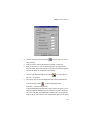
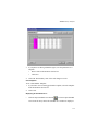
The Command menu contains two kinds of commands:
•
Commands that correspond to buttons on the Scan Control window.
•
Settings that affect the format and appearance of the scanned image.
These are displayed in the Scan Control window.
!
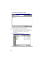
Before beginning a scan, check the following settings displayed in the Scan
Control window:
•
Gray Level Adjustment, including the Adjustment Type and the High
and Low Cutoff Thresholds
•
Image File Type
•
Orientation
6$:
Proper setting of the Gray Level Adjustment parameters enhances signal and
suppresses noise, resulting in clean, readable images. Improper setting of
these parameters might result in either saturated or faint images. The Gray
Level Adjustment parameters modify the signal intensity of each “dot,” or
pixel, in the scanned image. A pixel, is the smallest unit of a scanned image.
FMBIO Read Image files contain 16 bits per pixel, or 65,536 grayscale
levels (2' colors [black and white] = 65,536 shades of gray). Most computer
monitors are 8 bit and can therefore only display 256 (28) shades of gray.
4-10
FMBIO-Read Image Software
The Gray Level Adjustment tool tells your computer monitor how best to
display your image. It allows you to optimize your image by assigning these
256 shades of gray to the region of sample signal only. All pixels below the
sample signal range will be shown as white and all pixels above as black.
!"#"Cutoff thresholds are applied to the range of 216— or
65,536 — shades of gray that are generated during a scan. Background, or
noise, lies at the low end of this range; signal lies near the high end of this
range.
By adjusting the cutoff thresholds, you are adjusting the range between the
highest and the lowest acceptable gray shades. When the high cutoff is too
low, dark band images may be blurry, with indistinct edges. When the low
cutoff is too high, faint images are lost in the background.
When you change the percentages for high and low cutoff thresholds, you
change how the image appears on your monitor. You do not change how
much imaging data is collected. Once the image file has been saved, you can
use Image Analysis software to further experiment with the high and low
cutoff thresholds.
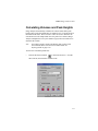
1.
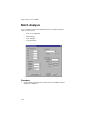
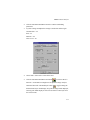
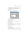
Choose Gray Level Adjustment... in the Command menu.
2.
Enter cutoff threshold values in the fields labeled Low (Background)
and High (Signal).
4-11
Read Image Software-FMBIO
3.
Click OK to save the Gray Level Adjustment settings.
-
The viewing orientation of the image can be changed in the saved file with
the Image Analysis software.
•
Choose Command > Orientation, then choose an orientation.
4-12
FMBIO-Read Image Software
(=
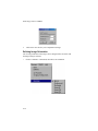
The FMBIO menu contains these commands:
•
Requesting an Autofocus before each scan
•
Determining which channels are active during a scan
•
Preparing the FMBIO scanning unit for cleaning
•
Ejecting the filter
!
During an autofocus, Read Image adjusts the focusing mirror and other
signal tracking and processing elements to find the best optical alignment.
This procedure takes approximately thirty seconds. After the initial autofocus, the procedure does not need to be repeated unless the scanning unit is
moved or bumped. The FMBIO always performs an autofocus at the
beginning of the first scan after the unit is turned on.
If you do not check the Auto Focus command, an autofocus occurs only
once, at the beginning of the first scan after you turn on the power switch,
which is on the front of the FMBIO scanning unit.
When a checkmark appears before the Auto Focus command, an autofocus
occurs before each scan.
The 605 nm filter should be in Channel 1 during the autofocus.
# # $%# #$Choose the parameter
settings and load a sample for a routine scan. When FMBIO completes the
4-13
Read Image Software-FMBIO
autofocus, it begins the scan. If Channel 1 is active, Read Image creates an
image file for the emission wavelength that passes through the 605 nm filter.
1.
Place the 605 nm filter in Channel 1. See page 3-6 for directions.
2.
Select Auto Focus in the FMBIO menu.
3.
Select the appropriate Read Image settings and load the sample.
4.
Click the Read button on the Scan Control window.
Before the FMBIO scanning unit begins the scan, it performs the autofocus.
Note
You can stop the scan after the autofocus. See page 3-12.
$"(
The FMBIO scanning unit has two optical filter holders and each filter
holder can hold two filters. As a result, the FMBIO scanning unit can simultaneously read four different emission wavelengths in the same lane or on an
entire gel.
Read Image collects emission data from all active channels during a scan.
Active channels are preceded by a checkmark in the FMBIO menu and are
listed in the Scan Control window. Channel 1 is the default active channel.
Note
Channel 1 does not have to be active if it is only in place for an
autofocus.
1.
Before beginning a scan, place the appropriate filters in the filter
holders.
2.
Choose the corresponding channels in the FMBIO menu to make them
active. Read Image collects emission data from each active channel
during the scan.
3.
Check the reading sensitivity setting for each active channel in the
FMBIO Parameter window. See page 4-8.
2
3
If you make a channel active in Read Image, the corresponding channel on
the FMBIO scanning unit must contain a filter. During a scan, if an active
channel does not contain a filter, or if the filter holder is not in place, the
resulting scanned image is white. If an active channel contains an opaque,
plastic barrier, the resulting scanned image is black.
4-14
FMBIO-Read Image Software
See Inserting Optical Filters on page 3-5 for directions on changing optical
filters.
See page 4-22 for information about the other commands in the FMBIO
menu.
"
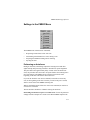
7
8
-
8
1 !
$
#
$
% #()%
)-
-
) -
-
$
-
$
4-15
Read Image Software-FMBIO
("
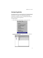
7
In addition to providing the tools for defining the scan area and performing
scans, the Scan Control window displays:
•
Scan settings specified in the Parameters window. See page 4-6.
•
Image file type, orientation, gray level adjustment—settings defined by
items in the Command menu. See page 4-10.
•
Autofocus and the active channels—settings defined by commands in
the FMBIO menu. See page 4-13.
4-16
FMBIO-Read Image Software
2
)
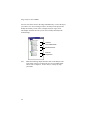
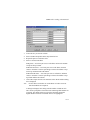
G '
$-
97!
-
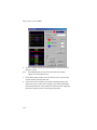
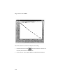
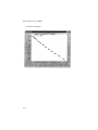
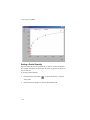
The PreRead Display in the Scan Control window represents the total scan
area of the FMBIO scanner bed. The material you are scanning is positioned
within the total scan area, but may be smaller than the total area. When there
is a rectangle inside the total scan area, it represents a pre-defined scan area
that is smaller than the total scan area.
!$
8
$
$-
When you choose PreRead, Read Image produces a low-resolution, rasterized image of the scan area in the PreRead Display. You can then modify
the scan area to include only essential information.
The total scan area is 200 mm x 430 mm. The minimum scan area is 20 mm
x 20 mm.
4-17
Read Image Software-FMBIO
Note
To reduce the file size of a scanned image, avoid including the glass
plate spacers and areas outside the sample in the scan area.
During a PreRead scan, the optical unit moves under the scanning bed and a
rasterized image begins to appear on the monitor.
To preview the entire scan area:
•
If the PreRead display is empty, the All Area button is not active. Click
the PreRead button to preview the entire scan area.
•
If the PreRead display contains a smaller, pre-defined scan area, the All
Area button is active. Click All Area to preview the entire scan area.
To preview a pre-defined scan area:
1.
Click the PreRead button to preview the pre-defined scan area.
2.
To redefine the scan area, place the cursor in the scan area and drag it to
the area of interest. You can change the size of the scan area by
dragging the sides of the rectangle.
"
You may enter memo information about the scan, such as date, researcher’s
name, or particular experiment features, in the Comment field in the Scan
Control window. The comment field holds up to 255 characters. Comments
are saved in a small text file associated with the image file. You can also use
Image Analysis to add comments to the image file.
*
When you have defined the scan area and all the scan settings, you can begin
scanning the sample.
•
To begin a scan, click the Read button.
Before the scan begins, a Save As dialog box appears. Use this window
to name the image and select its folder location.
When you click the Read button, Read Image estimates the size of the
image file that will be created and compares that size to available disk
space. If the amount of available free disk space is inadequate, an alert
box appears to warn you of insufficient space and Read Image cancels
the scan. If there is adequate disk space, the scan continues.
4-18
FMBIO-Read Image Software
Depending on the size of the image and the stringency of the scan parameters, scanning may take between five and ninety minutes. As the scan
progresses, a low-resolution raster image appears in the PreRead Display
window.
When scanning is complete the data is assembled into the digital image file.
This last step takes a short time.
4-19
Read Image Software-FMBIO
The menu bar in Read Image software contains many standard commands
found in IBM-compatible programs, as well as specific commands for operating the FMBIO scanning unit, modifying scan settings, and opening the
Image Analysis software. These additional features are discussed in this
section of the manual.
Most of the commands in the File menu are standard Windows commands.
&Opens a new Read Image file.
%Opens a saved Read Image file.
Closes the active Read Image file.
'Two commands in the File menu provide a way
to save Read Image files: Save and Save As. You can use these commands to
assign a unique name to a unique collection of settings that you plan to use
repeatedly.
$Files that have been opened recently are listed. Choose a file
to open it.
( Closes only the Read Image software.
4-20
FMBIO-Read Image Software
"
The Command menu contains commands to do the following:
•
correspond to buttons on the Scan Control window.
•
modify settings that appear in text on the Scan Control window.
See page 4-15 for information about the Scan Control window.
Corresponds to the Read button on the Scan Control window.
#Corresponds to the PreRead button on the Scan Control window.
##Corresponds to the Setting button on the Scan Control
window. Choose this command to open the FMBIO Parameters window.
)#'*+#For a discussion of these
commands, see page 4-10.
4-21
Read Image Software-FMBIO
=
The commands in the FMBIO menu directly manipulate the FMBIO
scanning unit. These commands only work if your system has been configured by qualified Hitachi Service personnel.
$See page 4-13 for a description of this command.
"Checkmarks precede the active channels. See page 4-13 for a
discussion of active channels.
,Moves the optical unit to allow access to the inside of the
scanning unit. You cannot change filters when the scanning unit is in the
cleaning position. See page 9-1 for more information about cleaning the
scanning unit.
*$# Moves the filter holders to make filters accessible for removal.
Note
4-22
Use the Eject Filter command only when the optical filter service
door is closed.
FMBIO-Read Image Software
=
In the scanning process, light signals are converted into a bitstream. The
FMBIO scanning unit generates 16 bit images. Each pixel in the image contains 216 or 65,536 possible signal intensity levels. 16 bit imaging can
produce very fine-grained images, in which very small or subtle differences
in the elements of the image may be discerned.
The resolution, or density of pixels (dots) in the digital image may be 75,
150, or 300 dots per inch (dpi) in each direction. Dot density of the image is
determined in Read Image before scanning.
Due to two limitations inherent in video display monitors, the image as it
appears on the monitor is a rough representation of the actual image data
present in the digital file. First, video monitors use 8 bit processing which
means only 28, or 256, signal intensity (gray scale) levels are displayed per
pixel. Thus file signals that are close but not identical to one another in grayscale value appear to have the same intensity on the monitor. Signals that are
slightly above the low cutoff threshold may also be submerged in background on the monitor.
Second, most video monitors have a resolution of 72 dpi. Thus an image
scanned at 150 x 300 dpi would contain 45,000 pixels/in2 in the digital file,
while the monitor is capable of displaying only about 72 x 72, or 5184,
pixels/in2. File pixels are averaged together for display purposes with a consequent loss of resolution, in this case at a resolution loss ratio of nearly 9:1.
The combined effect of these two limitations is that display images are apt to
appear coarser, grainier, or blurrier than they actually are.
You can compensate for these limitations in a number of ways:
•
Adjust gray scale and gamma controls to fit the particular conditions of
an image. With Image Analysis, you can modify the image to reveal a
very broad range of signal intensities. Just remember that considerably
more information is latent in the image than can be displayed with any
particular set of display parameters.
•
Many factors contribute to the success of DNA detection. Variables
include: gel type and concentration, sample preparation, band size, dye
concentration, staining time, destaining time, gray level settings, and
laser focusing point. Further optimization of protocols may result in
higher detection sensitivity.
4-23
Read Image Software-FMBIO
•
For best scanning results, avoid dust specks by using only powderless
gloves, rinsing gloves with distilled water, thoroughly cleaning all
containers used for staining, and filtering all buffers and solutions with a
0.45 µm filter.
•
Loading buffers containing xylene cyanol and bromophenol blue
fluoresce strongly when excited by the FMBIO laser, and can interfere
with the gel image. For best results, use loading buffers containing no
xylene cyanol, and bromophenol blue concentrations decreased 1:10.
•
Gels can be cast with ethidium bromide to save time after
electrophoresis. However, electrophoretic mobility of linear doublestranded DNA is reduced by up to 15% in the presence of ethidium
bromide and background staining is not uniform when casting agarose
gels with ethidium bromide. Therefore, post-staining is highly
recommended.
•
Detection sensitivity is higher in acrylamide gels than in agarose gels,
due to lower background.
•
Ethidium bromide can be used to detect both single-and double-stranded
DNA or RNA. The affinity for double-stranded DNA is higher than for
single-stranded DNA or RNA.
•
Longer staining times do not necessarily increase sensitivity.
•
Shortening the ethidium bromide staining time or lengthening the water
destaining time may decrease detection sensitivity.
•
Keep all solutions containing ethidium bromide covered by aluminum
foil to prevent bleaching of the dye by ambient light.
•
Ethidium bromide is a powerful mutagen. Follow usage precautions as
described on the MSDS.
4-24
FMBIO-Read Image Software
%"
Multi-wavelength analysis makes it possible to create and analyze signals
from multi-color gel images. Two or more fluorophores of different emission
spectra can be run in the same lanes, or on the same gel. This function is
useful for comparative allele analysis, or for highly accurate size determination by running a marker in the same lane with a sample.
To scan material with more than one emission wavelength requires that you
scan with multiple channels, with the appropriate filters in place.
Multi-color analysis depends on the use of appropriate filters. Each filter
captures one emission wavelength by screening out the others. To load
filters, see page 3-5.
6!
Long pass filters reject shorter wavelength light while allowing longer wavelengths to pass through. Long pass filters are named for the wavelength at the
midpoint of the transition range, for example, OG 610. The midpoint of the
sigmoid curve that describes the transition from 0 to maximum transmission.
The narrower this transition range is, the better, especially when the two fluorophore emission frequencies are close.
The name of the long pass filter may also include letters such as OG (orange
glass), RG (red glass), E (emission), LP (long pass), EFLP (edge filter long
pass). OG and RG are colored glass absorption filters, whereas E, LP, and
EFLP filters are coated interference filters. Colored glass filters are cheaper
and have broader transition slopes than coated interference filters.
Match filters to fluorophores in such a way as to maximize the amount of
signal separation. This multi-color image contains red, green and blue
signals, which were created with FITC, TMR and CXR dyes matched with
505, 585 and 650 filters, respectively.
4-25
Read Image Software-FMBIO
4-26
FMBIO-Read Image Software
!
This section describes the process of scanning, using as an example the
detection of fluorophore-labeled str alleles.
7*889
!
(<(
(
(
(
<
(
$=
<
1.
Turn on power to the computer.
2.
Turn on power to the FMBIO. (The switch is behind the pull-down
panel, on the front left).
3.
After electrophoresis has been performed, keep the polyacrylamide gelplate assembly together. Carefully clean and dry the outside of the
plates. The gel-plate assembly does not need to be taken apart, unless
post-staining is necessary for your application.
Note
Maintaining the integrity of the gel-plate assembly can allow for
better separation of larger STR loci, because the gel can be returned
to the electrophoretic apparatus after scanning for additional
electrophoresis.
If you have an agarose gel, polyacrylamide mini-gel or membrane, place
them on a 5 mm thick, low-fluorescent glass plate. Avoid dripping by
removing excess buffer on stain. Smooth out bubbles under gels, as they
can interfere with the scan. Membranes should be mounted wet, face
down between two pieces of glass. Polystyrene and other clear plastics
may also be acceptable for holding sample(s), but may result in high
levels of background.
4.
Place the gel-plate assembly in the scanner.
a.
Press the button on the top right of the front of the instrument, and
open the sample door.
b.
Slide the right side stage bar to the proper distance to support the
plate, without obscuring the area to be scanned.
c.
Place the plate assembly (long plate face down) on the stage, resting
the plate assembly on the black bars at each end and between both
of the stabilizing screws on the bars. Make sure the plate is level
4-27
Read Image Software-FMBIO
and secure. For polyacrylamide gels, place long plate face down.
5.
Start the FMBIO Read Image program.
6.
Click the Setting button. The Read Image Parameter dialog box is
displayed.
7.
Set the Scanning parameters:
Note
The example show described below is for illustration only, and must
not be interpreted as a suitable procedure for any particular case.
a.
Choose the Parameter Name. In this example Acrylamide is
entered.
b.
Choose the resolution. 150 dpi is an example for the initial setting.
c.
Enter the sensitivity. In this example, 80% is entered for Channels 1
and 3, and 100% for Channels 2 and 4. One of the factors
influencing this choice is the filter types used.
d.
Enter the focusing. 0 is shown in this example. It may need to be
lower for the thinner plates used in pre-cast gels. Note that the
range of focusing is ONLY - 2 mm to + 3 mm. Use of values
outside of this range can seriously damage the instrument.
e.
Choose the number of repeats. An initial setting example is 256.
4-28
FMBIO-Read Image Software
a.
Click OK to return to the Scan Control window.
8.
In the FMBIO menu, set the active channels. A separate image is
collected for each channel.
9.
Since the instrument will always autofocus before the first read after
power-up, turn Auto Focus off in the FMBIO menu to save time during
subsequent scans. The 605 nm filter must be installed in Channel 1 for
autofocusing.
10. In the Command menu, set the gray level adjustment for
polyacrylamide gels. Examples might be 50% for Low and 1% for
High.
11. Make any changes needed to Orientation in the Command menu.
Note
To save the Read Image parameters for future scans, choose Save
from the File menu, assign a filename and location, and then click
Save. Double-click on the saved parameter file to launch the Read
Image program and return the user to the saved scanning
parameters.
4-29
Read Image Software-FMBIO
12. Add any comments to an image file by typing those comments in the
text box in the lower section of the Scan Control window.
13. Click the PreRead button to quickly identify the gel area to scan.
Note
If a small scanning box is already set from a previous scan, click on
the All Area button before prereading. If you need to terminate an
in-progress prereading, click Cancel.
14. Designate the scan area by dragging with the mouse from top left to
lower right in the viewing window.
Note
4-30
DO NOT include SPACERS or other solid objects in this box,
because they can distort the gray scale balance of the image.
FMBIO-Read Image Software
15.
Note
Click Read. Specify a file name, and a location for the saved file.
You can terminate a scan before completion by clicking Cancel,
then save or discard the image data.
16. Wait for the instrument to complete all of its scans. The FMBIO will
autofocus and might scan twice depending on the channels chosen.
After the scan begins, a calculated time for completion is noted in the
lower right of the Read Image Window. This time is per scan, and
calculation accuracy improves as the scan progresses.
17. To view the results, use the Image Analysis software.
18. Adjust the gray scale to optimize the image.
Note
See Gray Level Adjustment on page 5-13 for information about gray
scale adjustment.
19. If the image is satisfactory, proceed to Chapter 5.
20. If the gray scale adjustment does not produce an adequate image, make
the adjustments suggested in the Image Troubleshooting Guide at the
end of this chapter, then rescan the image.
)%#2(
!
:
N
8
,
*
;):
C
N
7
N
N
N
7
N
N
N
7
N
N
N
7
4-31
Read Image Software-FMBIO
*"
In the process of using Read Image software, you may occasionally see an
error code number appear on the screen.
###$-./.+./0+./1+./2+./3+./4+#./5Perform the following
steps:
1.
Press the Power switch to the Off position and wait at least 5 seconds.
2.
Press the Power switch to the On position.
The FMBIO performs a self-diagnostic routine.
•
3.
If the error code appears again, repeat steps 1 and 2 one more time.
If the error code persists, call Hitachi Software Engineering service
personnel.
###$-.// Insert a filter holder in either Channel 1 or Channel 2,
and then restart the scan.
###$-./6Firmly close the scanning unit cover.
###$-.50There is an internal memory shortage.
###$-.51There is an external memory shortage.
###$-.56The optical unit did not return to the home position.
4-32
+ With the FMBIO scanning unit and Read Image software, a single scan can
create a multi-color image of a gel that contains one, two, or more fluorophores in one scan. In Image Analysis, you can view and analyze the scanned
image.
You can run fluorophores of two or more different emission spectra in the
same lane or gel for comparative allele analysis. Highly accurate size determinations can be achieved when an internal lane standard is run in the same
lane with a sample. If a sample contains two or more fluorophores and you
designate two or more channels as active during the scan, FMBIO Read
Image creates a multi-color image.
In Image Analysis, you create a project to analyze your 1D or array experiments. You can create a project for a single- or multi-color image. You can
also display images and data from more than one project simultaneously.
5-1
Image Analysis Tools-FMBIO
You can view all the colors in the image simultaneously, or select the layers
you want to view. You can assign a color to each layer in the project and
modify the intensity of each color, or display all layers in gray scale.
This chapter describes the tools you can use to modify and analyze the
scanned image.
-
,L)1
$-
-
1
Note
5-2
While the following chapter describes each of the analysis tools
in the order of use it is not meant to serve as a procedural guide.
Please refer to Chapter 6, 1D-Gel Analysis, for step-by-step
procedures.
FMBIO-Image Analysis Tools
!:
Double-click the Image Analysis shortcut icon to start the Image Analysis
program. When the Image Analysis window opens, a new project is automatically created for you and a new Project window is displayed.
You can use this new project, create another new project, or open an existing
project.
"
8!:
•
To create a new project, click the New Project button
or choose
New Project from the File menu.
!:
•
To open an existing project, click the Open Project button
or
choose Open Project from the File menu.
$!:
•
To save a project, click the Save Project button
or choose Save
Project from the File menu. Give the project a name and click Save.
5-3
Image Analysis Tools-FMBIO
1.
In the Project menu, choose New 1D-Gel Experiment or New Array
Experiment.
2.
Select an image file from the directory window. The image icon is
added to the project tree.
3.
Double-click the image icon to display the selected image.
Once an image is displayed, the Image menu appears in the menu bar and the
Image tool buttons become active.
5-4
FMBIO-Image Analysis Tools
*,7
-
$ $
$1
"
-
*,7
$
!
-
$ $
!+5
$
$1
$
!
!
9 G
!
#()%
$
$
8##
)($
!6
5-5
Image Analysis Tools-FMBIO
"
-
8 ):
$"
#
!
,$
1
$
1
$
$ $#
!+
In addition, you can use the Zoom tools to magnify or reduce the image.
O
%
O
8
O
#
(
8
(
C,)
'
-
O
%
3:
O
3:
(
C,)
'
1 3
!
!
5-6
FMBIO-Image Analysis Tools
O
8
-
-:
8
PMQ
+
1
8
#
%
G
(
8
-:
G
$
You can save the entire image or a selected area of an image as a TIFF or
BMP file.
1.
If you want to crop the image, click the Select area to draw button
or choose Area Selection from the Image menu. Place the crosshair
pointer on a corner of the rectangular area you want to save, and clickand-drag the mouse to the opposite corner of the area. Release the
mouse.
2.
Choose Save Image as... from the Image menu. The Save Image as
5-7
Image Analysis Tools-FMBIO
dialog box is displayed.
!
-
$<
$
$
$
8 8##
)(
*
2
G4G+6G
/
)
4
/
-
$
G+G0
-
$ G
= !
>
#
# <
5-8
FMBIO-Image Analysis Tools
!
)(#
-
$
G
:
3.
Select the appropriate parameter settings, and click OK. The Save As
dialog box is displayed.
4.
Specify a location for the file in the Directory window, and enter a
filename.
5.
Click the Save button.
A
%"
A multi-color image is a combination of two or more scanned image channels that share the same scan area and orientation. FMBIO Read Image
automatically creates a multi-color image file whenever two or more channels are active during a scan. When Image Analysis opens the image file, it
displays the combined image channels as one multi-color image.
1.
Click the folder expansion
symbol next to the image icon to display
the names of each layer in the image.
2.
In this example, during one multi-color scan CTTv, DDDD, and InlaneCXR were the active channels.
5-9
Image Analysis Tools-FMBIO
-=
You use the Image Setting dialog box to change how the image is displayed
on the screen.
•
By default the Image Setting dialog box is displayed. If it is not displayed, click the Show mage Setting Dialog button
or choose
Show Image Setting Dialog from the Image menu. A checkmark indicates the dialog box is displayed.
The Image Setting dialog box looks like this:
*
,
7
5-10
FMBIO-Image Analysis Tools
Note
The Show color-separated images option is active only after you
have performed a color separation on the image. See Color Separation on page 5-29.
-
The Image Setting dialog box assigns a unique color to each channel in the
multi-color image. The colors available depend on the display mode. The
Display Mode list box provides three options: Blend, Over, and Mono. Use
the Display Mode drop-down list box to choose how you want a multi-color
image displayed. The colors available in the Image Setting dialog box
change as the display mode option changes.
"$
)
G*G). -
:
:
E
:E
:
%
G*G)GH
-
!
.
!
7
(
/G
!
-"(
You can choose to display or hide the image data from one or more channels.
•
Select the channel to show the channel image data. To hide a channel’s
image data, remove the checkmark adjacent to the channel.
Note
You cannot turn off the channel display in Mono display mode.
"("("
You can change the color associated with a channel in the multi-color image.
The Color Chooser is the colored square next to the channel name. No two
channels may have the same color assignment.
•
Click the Color Chooser for the channel you want to change. A pop-up
menu of available colors is displayed. Click the desired color.
5-11
Image Analysis Tools-FMBIO
"(
6$
You can change the intensity of each color associated with a channel.
•
Drag the gamma level bar to the right to increase intensity. Slide the bar
to the left to decrease intensity.
--
=
After you use Image Analysis to define bands on all channels, you can
choose which channel displays the band definition lines.
•
Click the radio button adjacent to the channel name. The black dot in the
radio button indicates the active channel. In the image, Image Analysis
displays the band definition lines for the active channel.
For more information on detecting bands, see page 5-60.
5-12
FMBIO-Image Analysis Tools
6$:
The proper setting of the Gray Level Adjustment parameters enhances signal
and suppresses noise, resulting in clean, readable images. Conversely,
improper settings might result in either saturated or faint images.
The Gray Level Adjustment parameters modify the signal intensity of each
“dot,” or pixel, in the scanned image. A pixel, is the smallest unit of a
scanned image and each channel in an FMBIO II file contains 16 bits per
pixel, or 216=65,535 grayscale levels (starting at 0). Most computer monitors
are 8 bit and can therefore only display 256 shades of gray.
Image Analysis transforms the 16 bit image for display on an 8 bit monitor,
averaging the additional 16 bit values within each of the 256 8 bit grayscale
levels to give an 8 bit value. The Gray Level Adjustment tool tells your
computer monitor how best to display your image. It allows you to optimize
your image by assigning these 256 shades of gray to only the region
containing sample signal.
Note
The raw image data is not affected by the gray level settings.
Cutoff Thresholds. Image Analysis assigns a background cutoff threshold
and a high signal cutoff threshold for each image. Cutoff thresholds are
applied to the range of 65,536 shades of gray generated during a scan. Background, or noise, lies at the low end of this range; signal lies near the high
end of this range.
Signals below the background cutoff threshold appear white in the image;
signals above the high signal cutoff threshold appear as black. The range
between the background and high signal cutoff thresholds signals is transformed into 256 gray levels.
5-13
Image Analysis Tools-FMBIO
To obtain greater clarity of an entire image or certain selected bands within
it, you can modify the range of gray levels in each channel. In the Gray
Level Adjustment window, you can use a histogram to adjust the cutoff
threshold values. Alternatively, you can designate reference background and
high signal areas on the scanned image. Using these reference areas, Image
Analysis automatically adjusts all gray levels on the image.
By adjusting the cutoff thresholds, you are adjusting the range between the
highest and the lowest acceptable gray shades. When the high signal cutoff is
too low, dark band images may be blurry, with indistinct edges. When the
background cutoff is too high, faint images are lost.
Because signal intensities can vary greatly from one scan to the next, it is
difficult to assign default values for high signal and background cutoff
thresholds. Images that contain only faint bands against a clean background
can be enhanced with high signal and background cutoff thresholds set to
relatively high values. Images that contain heavily stained or optically dense
regions may suffer substantial loss of content even with low threshold
values.
The diagnostic guide on page 5-24 provides guidelines for threshold adjustment. See also Imaging Basics on page 4-23.
5-14
FMBIO-Image Analysis Tools
:
5-15
Image Analysis Tools-FMBIO
6$:
7
Click the Gray Level Adjustment button
or choose Gray Level
Adjustment from the Image menu. The Gray Level Adjustment window is
displayed.
Channel Selector.
The gray level must be adjusted for each individual channel. Select the
channel from the Channel drop-down list box. The Gray Level Adjustment
window displays the image data for the selected channel.
Background and High Signal cutoff thresholds.
The values in the High Signal Percent and High Signal Number fields
change to reflect the selected region. In the following example, 1.85% of the
pixels have a value between 4,081 and 65,535. These pixels will appear on
the monitor as black.
5-16
FMBIO-Image Analysis Tools
All regions of the image with gray level values below the background cutoff
threshold value will appear white. As shown, 90.44% of the pixels have a
value between 0 and 1,537. These pixels will appear on the monitor as white.
All other elements of the image that fall within the range between the high
signal and background cutoff thresholds appear as shades of gray.
Histogram.
R
'
The Gray Level Histogram shows the 16 bit gray level gradations (0 to
65,535) on the X axis and the number of pixels in the image on the Y axis.
Boundary lines indicate the high signal cutoff threshold and background
cutoff threshold. The red line slider indicates the background cutoff
threshold value. The blue line slider shows the high signal cutoff threshold
value. The green line on the histogram displays the current mapping curve.
By default, the mapping curve is displayed.
5-17
Image Analysis Tools-FMBIO
(
):
8
-
;$8
Show Selected Range. 3
Mapping Type Selector.
The mapping type defines the method used to translate 16 bit gradation (0 to
65535) into 8 bit gradation (0 to 255). The gray level gradations between the
high signal cutoff threshold and the background cutoff threshold are divided
into 255 equal parts. To view the mapping curve, select the Show Mapping
Curve option.
5-18
FMBIO-Image Analysis Tools
3@
-
N
:
+/@ 2
&.3@
3@
N
:
+/@ 2
&.3@
E
2%8
5-19
Image Analysis Tools-FMBIO
.1
-
N
1
2
&..1
<
!
The gray level for each channel is adjusted by setting the background and
high signal cutoff thresholds. You can set these thresholds in three different
ways:
•
Drag threshold boundary lines in the histogram.
•
Visually defining signal and background pixels.
•
Entering numbers for the high signal and background values.
Using the histogram.
1.
Select a channel and mapping type.
2.
To adjust the high signal cutoff threshold value, place the pointer over
the blue line. The pointer transforms into a horizontal double-headed
arrow.
3.
Drag the line along the gray level axis until the desired value is displayed. The new high signal cutoff threshold value is applied to the
Whole Image and Zoomed Area windows and a new High Signal
Percent value is calculated.
4.
To adjust the background cutoff threshold value, place the pointer over
5-20
FMBIO-Image Analysis Tools
the red line. The pointer transforms into a horizontal double-headed
arrow and the value appears in the upper left corner of the window.
5.
Drag the line along the gray level axis until the desired value appears.
The new background cutoff threshold value is applied to the Whole
Image and Zoomed Area windows and a new High Signal Percent value
is calculated.
6.
Click the Try button to apply the modified gray levels to the actual
image. To return to the original settings, click Reset.
7.
Continue to try different gray level settings until you are satisfied with
the signal and background levels.
8.
Repeat the procedure for each channel.
9.
When you are finished, click OK.
Image Analysis recalculates the gray levels for the channels using these
values as high signal and background limits.
Note
The raw image data is not affected by the gray level settings.
Visually defining signal and background pixels. You can define the signal
and background intensities using the Zoom and Selection cursors.
O
-
$
-
1.
Select a channel and mapping type.
2.
In the Whole Image window, drag the Zoom Cursor to a region con-
5-21
Image Analysis Tools-FMBIO
taining average intensity bands/background. If necessary, adjust the size
of the Zoom Cursor to include the desired area. The area appears in the
Zoomed Area.
3.
In the Zoom window, surround a band with the Selection Cursor.
4.
Click the High Signal button. The image displays appear with the new
high signal cutoff threshold and the values are displayed in the High
Signal Percent and High Signal Number fields.
5.
Move the Selection Cursor to a background area away from the band.
6.
Click the Background button. The selected background cutoff threshold
is applied to the Whole Image and Zoomed Area windows and the
values appear in the Background Percent and Background Number
fields.
7.
Click the Try button to apply the modified gray levels to the actual
image. To return to the original settings, click Reset.
8.
Continue to try different gray level settings until you are satisfied with
the signal and background levels.
9.
Repeat the procedure for each channel.
10. When you are finished, click OK.
Image Analysis recalculates the gray levels for the entire image using these
values as high signal and background limits.
Note
5-22
The raw image data is not affected by the gray level settings
FMBIO-Image Analysis Tools
Using the percent and number fields.
You can also adjust the high signal and background cutoff thresholds by
entering values in the percent and number fields.
Select a channel and mapping type.
1.
Enter numbers in either the percent or absolute value fields, and then
click OK.
2.
Click the Try button to apply the modified gray levels to the actual
image. To return to the original settings, click Reset.
3.
Continue to try different gray level settings until you are satisfied with
the signal and background levels.
4.
Repeat the procedure for each channel.
5.
When you are finished, click OK.
Image Analysis recalculates the gray levels for the entire image using these
values as high signal and background limits.
Creating a template.
If you have a series of gels that have been run under the same conditions and
produce similar images, you might want to save your gray level adjustment
values as a template for future use:
1.
Click the Template button.
2.
Click the Create New button. The Template dialog box is displayed.
3.
Type a unique name for the template, then click the Close button.
Note
When a Gray level Adjustment Template is created, only the
mapping type, high signal cutoff threshold value, and background cutoff threshold value are saved. The percent values are
not saved. Therefore, it is imperative that a Gray Level
Adjustment template is created for each channel.
To apply a gray level adjustment template:
1.
Select a channel.
2.
Click the Template button.
3.
Select the template name, then click the Apply button.
5-23
Image Analysis Tools-FMBIO
-
E
"
((
3
:
:
3
1:
:
:
:
1:
G
1:
:
+/
8
'
:
$
7=
G
G
>
G;
$
3
8
G!
7
If, after these steps, you cannot achieve a satisfactory image, you may have
too much signal. Try rescanning the sample at a lower photomultiplier tube
(PMT) sensitivity, scan using a different filter or, if stains were used, destain
the gel.
5-24
FMBIO-Image Analysis Tools
With the FMBIO system you can accurately signal strength at particular
locations on the image. This quantification is more accurate than conventional radiography followed by scanning densitometry because the
intermediate film and scanning steps are eliminated. The FMBIO spectrum
function analyzes the pixel and gray scale data in the digital image and calculates the signal strength at a given location.
You can use two methods to select the location on the image for spectrum
analysis.
•
Draw a rectangle on the image. The spectrum displays the signal strength of the bands within the rectangle.
•
Draw a straight line on the image. The spectrum displays the
signal strength at each point on the line.
(
1.
Click the Area Selection button
or choose Area Selection from the
Image menu.
2.
Position the tool at a corner of the group of bands you want to select.
Drag the cursor down to the opposite corner until the bands are contained in the rectangle.
3.
Release the mouse button. A selection rectangle is displayed. If necessary, adjust the rectangle by dragging the selection handles.
5-25
Image Analysis Tools-FMBIO
4.
Click the Spectrum View Button
or choose Show Spectrum from
the Image menu. The Spectrum window displays an overlay trace of the
signals, with the areas of signal intensity represented by peaks.
Normalize Baseline
Display Channel
Switch Axis
5-26
FMBIO-Image Analysis Tools
-
2
<)
2
<
$'
$
<
1 -
8
5.
To change the dimensions of the graph, resize the window.
Normalize Baseline tool. Click the Normalize Baseline tool to normalize
the vertical range by converting the low end of the range to 0 (zero) and the
upper end of the range to 255. Use this feature to compare lane traces from
different image files or from files created by different filters.
Before the vertical range is normalized, it represents the range between the
high and low Cutoff Thresholds on the Gray Level correction. The low and
high ends of the vertical range before normalization lie somewhere within
the range of available pixels in a 16 bit file, from 0 to 65, 535. On this range,
spots on the image that appear black or “saturated” may actually have a
signal above the high cutoff threshold.
However, when the vertical range is normalized, it is compressed to fit to the
range of available pixels in an 8 bit file, from 0 to 255. The low cutoff
threshold becomes 0; the high cutoff threshold becomes 255. When Image
Analysis encounters signal above the high cutoff threshold, it extrapolates a
value for these spots that may actually be greater than 255. The upper end of
the vertical range reflects the value assigned to these high signals.
(
6
(
1.
Click the Area Selection button
or choose Line Selection from the
Image menu.
2.
Drag the cursor in a straight line over the location you want to analyze.
3.
Release the mouse button. A selection line is displayed. If necessary,
adjust the line by dragging the selection handles.
5-27
Image Analysis Tools-FMBIO
4.
Click the Spectrum View button
the Image menu.
5-28
or choose Show Spectrum from
FMBIO-Image Analysis Tools
"
In multi-color fluorescence imaging, up to four fluorescent dyes (fluorophores) can be detected in a single image. Although each fluorophore
exhibits its own characteristic emission spectrum, with a distinct maximum
at specific wavelength, there may be some overlap (bleed-through) between
the spectra of the different fluorophores.
The purpose of color separation is to identify these areas of emission spectra
overlap by quantifying the proportion of each fluorophore that is known to
overlap with the other fluorophores.
Image Analysis allows two methods for color separation:
•
Color separation by individual band selection
•
Multi-band color separation
Multi-band color separation is a feature of the 1D-Gel analysis tools. See
page 5-41.
"
(
The following is a theoretical treatment of color separation for an image with
two channels. Below are shown the spectra for an image from a lane with
two channels. In this example, the pixels in region B of Channel 2, bleed
through into area A of Channel 1 so the following type of color separation is
performed.
5-29
Image Analysis Tools-FMBIO
Remove the background portion (N1, N2) from each channel.
1.
Calculate the bleed-through rate:
Bleed-through rate RAB=SA/SB
2.
The bleed-through rate (RAB) is calculated for each pixel value in
Channel 2 and the corresponding pixel value in Channel 1. This rate is
multiplied by the image pixel values in Channel 2, and the result is subtracted. Then the spectra in Channel 2 is as follows:
For any point on the image P(x,y), the image pixel value in Channel 1 is
I1 and the image pixel value in Channel 2 is I2. After color separation,
the pixel value in Channel 1 is:
I2 = I2 - (I1-N1) x RAB, provided (I1-N1)>0
3.
The operations explained above for Channel 1 are the applied to
Channel 2.
5-30
FMBIO-Image Analysis Tools
$="
To separate the colors in an image using individual bands, you must select at
least one non-overlapping, medium intensity, representative band of each
color.
1.
Click the Color Separation button
or choose Color Separation
from the Image menu.
The Color Separation window is displayed.
5-31
Image Analysis Tools-FMBIO
2.
Choose a channel from the Selected Fluorophore drop-down list box,
and select a color.
Note
In the Blend mode, the color associated with each channel
appears in the box adjacent to it.
3.
In the Whole Image window, move the Zoom Cursor to an area with
medium intensity bands of that color.
4.
In the Zoomed Area window, pick a band of medium intensity that
matches the color, but does not overlap any other band. Surround the
band with the Selection Cursor. Make the Selection Cursor larger than
the band to include a portion of the image background.
5-32
FMBIO-Image Analysis Tools
O
O
$
5.
Click the Set button to make the color of the selected band represent the
fluorophore. Image Analysis calculates the percent overlap between
selected fluorophore and each of the other channels. The percentages are
displayed in the Emission Overlap fields.
•
You can click the Preview button at any time to test the color
separation process.
•
Click the Original button to revert to the original color settings.
6.
Use one of the other channels in the Selected Fluorophore list.
7.
Repeat this process for each of the remaining channels.
8.
If the Color Separation parameters are to be used again in the future,
click the Template... button. Click Add... and assign the template a
unique name.
9.
When you are satisfied with the color settings, click OK.
10. If you want to remove the color separation, uncheck the Show ColorSeparated Images, checkbox in the Image Setting box. You can now
repeat the color separation process.
5-33
Image Analysis Tools-FMBIO
"
To perform this function a previously created Color Separation template
must have been saved.
1.
Click the Color Separation button
or choose Color Separation...
from the Image menu.
2.
Once the Color Separation window has opened click the Template...
button. The Template dialog box is displayed.
3.
Select a template, then click the Apply button.
4.
Click Close.
5.
Click OK. The selected Color Separation template is applied to the new
image.
"
*
On some gel images, the color separation process can result in over-subtraction of a dye that has minimal bleed-through signal.
For example, a gel image might contain three dyes: tetramethyl rhodamine,
carboxy-x-rhodamine, and fluorescein. The two rhodamine derivatives have
overlapping emission curves, but fluorescein has minimal overlap with the
other two dyes. The following procedure explains how to exclude the nonoverlapping dye, fluorescein, from the color separation process.
1.
In the Image Setting dialog box, turn off the Show color-separated
images option.
When the option is off, the checkbox is empty.
2.
Click the Color Separation button
or choose Color Separation...
from the Image menu.
3.
Choose one of the overlapping dyes (carboxy-x-rhodamine) from the
Selected Fluorophore drop-down list.
4.
In the Target Channel section, enter a zero (0) in both the Background
and Percent entry fields for the fluorescein channel.
5.
In the Mode section, click Preview to examine the new values in the
Whole Image window and Zoom window. You may see a slight color
5-34
FMBIO-Image Analysis Tools
change.
6.
In the Selected Fluorophore list, use the drop-down list to choose the
second overlapping dye (tetramethyl rhodamine).
7.
Enter a zero (0) in both the Background and fluorescein Percent entry
fields.
8.
Preview the color separation.
If you are satisfied with the results, click OK on the Color Separation
box. When the message “Create the Separated Images this time?”
appears, click OK again.
9.
If you want to remove the color separation, uncheck the Show ColorSeparated Images, checkbox in the Image Setting dialog box. You can
now repeat the color separation process.
= You can choose to make the background of an image transparent and position
it over another image to compare bands.
To make the background of an image transparent, select Transparent Background from the Image menu.
5-35
Image Analysis Tools-FMBIO
5-36
FMBIO-Image Analysis Tools
#-%
1.
Click the New Project button or choose New Project from the File menu.
2.
Choose New 1D-Gel Experiment from the Project menu.
The 1D-Gel Experiment window, Image Setting dialog box, 1D-Gel
menu and its corresponding tool bar appear.
5-37
Image Analysis Tools-FMBIO
Overlay Trace
Set Marker
Volume Calculation
Open Spreadsheet
Multi-Band Color Separation
Preferences
Quantification Setting
Open BP Curve
-
%8
1 $(:
1 (:$
9
-
% $ 1 % )$-
1 ?
$
1 ?
$
1 (!)
-
$ 1 (!)-
$ 5-38
FMBIO-Image Analysis Tools
,$
8
( ,$
8
,8 )1
)3
1)
,#
$8
,
-
$8
$
7
,$
8
1
( ,$
1 7
,8
,#
7
,8 - )1
1
1)
1
)3
GG
5-39
Image Analysis Tools-FMBIO
$
C;,
$
C;)
$
C;-
)$
,$
-
$
C;,
8
$
C;
)
8
GG
%1G((G) $
C;
-
8
,$
8
&
G
G
G!
)$
8
&
G :
G
:!
5-40
FMBIO-Image Analysis Tools
%="
In a 1D-Gel Analysis, Image Analysis lets you perform separation all colors
simultaneously using multiple bands within a lane. The colors assigned to
the bands collectively constitute a Multi-Band Separation Parameter Set,
which is used to calculate the spectral overlap between the individual
fluorophores.
=
!
Before performing multi-band color separation can be performed, you assign
values for the Band Selection Parameters, which define the criteria for calculating the background, band area, and overlap between bands in a lane.
1.
Choose New 1D-Gel Experiment from the Project menu.
The 1D-Gel Experiment window, Image Setting dialog box, 1D-Gel
menu and its corresponding tool bar appear.
2.
Click the Preferences button
or choose Preferences... from the
1D-Gel menu.
3.
Click the Multi-Band Color Separation tab. This filecard displays the
default Band Selection Parameter set.
4.
Try these settings and, if necessary, adjust them for different gels:
•
Overlap = 0.0 mm
•
Band Area = 0.1 mm
•
Background Area 1 = 0.5 mm
•
Background Area 2 = 0.5 mm
•
Background % = 100%
Note
If you plan to use these parameter settings in the future, it is necessary to save a template with a unique name.
5-41
Image Analysis Tools-FMBIO
Overlap. Specifies the width of the band used in the area calculation when
checking for band overlap.
•
If this Overlap value is 0.0 mm, the overlap will be the width
detected by the Auto Band tool.
•
If there is no overlap, the band area is the total that is calculated by the Auto Band tool.
•
When the Overlap value (X) is greater than 0 mm the width
used to calculate the area will -X to +X from the peak maximum.
•
Overlap values may range from 0-99.9 mm with a minimum
increment of 0.1 mm.
5-42
FMBIO-Image Analysis Tools
Band Area. Specifies the area that is used to calculate the volume for color
separation.
•
If this Band Area value is 0 mm, the band area will be the area
detected by the Auto Band tool.
•
If the Band Area value (X) is greater than 0 mm the band area
will be -X to +X from the peak maximum.
•
Band Area values may range from 0 to 99.9 mm with a minimum increment of 0.1 mm.
Background Area 1. The area directly adjacent to either side of the band of
interest that is used in the background calculation.
Background Area 2. The area between bands of interest that is used in the
background calculation.
5-43
Image Analysis Tools-FMBIO
Background %. Specifies the correction value for the calculated background value. This Background % value should range from 1 to 100%.
%="
7
To use the multi-band color separation window, you must select a lane
containing a minimum of one medium intensity band of each color.
1.
Find a portion of a lane containing a minimum of one non-overlapping
band of each color.
Note
2.
Two or more bands of each color is recommended.
Click the Lane Selection Tool button
or choose 1D-
Gel>Tool>Lane Selection. Drag down and then across that portion of
the lane.
3.
Click the Automatic Band Detection button
or choose 1D-Gel >
Function > Auto Band.
Note
5-44
Auto Band detects bands in all channels. To view the detected
bands in a channel, select the channel in the Image Setting
dialog box. See Displaying Detected Bands on page 5-12.
FMBIO-Image Analysis Tools
4.
After Image Analysis has autobanded the lane, click the Multi-Band
Color Separation button
or choose Multi-Band Color
Separation... from the 1D-Gel menu. Using the Band Merging parameters, Image Analysis assigns a color to each band, and the Multi-Band
Color Separation window is displayed.
,$
,
(
$
5-45
Image Analysis Tools-FMBIO
1)2
)
,8
,
Lane Window. The Lane window displays all detected bands and a spectrum trace of the selected lane. The color of the Detected Band number
indicates the color assigned by Image Analysis.
):
(:
Magnification Selector. To view the Lane window at a higher magnification, select a percent value from the drop-down list box.
5.
If you are not satisfied with the separation of the colors, you can adjust
the Multi-Band Color Separation preferences. Click the Set Multi-Band
Parameters...button, and change the parameter values. When you click
OK, the colors are automatically separated according to the new values.
5-46
FMBIO-Image Analysis Tools
6.
On the right side of the window the Status Edit Sheet displays the
detected band numbers.
•
If you want to use the colors assigned by the Multi-Band Color
Separator, click the Copy==> button.
•
If you want to load a previously saved Multi-Band Separation
template, click Template...Select a template, and then click
Apply. The detected bands appear in the Status Edit Sheet.
$38
1)
2
7.
Review each band in the Status Edit Sheet, verifying that the assigned
colors are representative of the colors viewed in the gel image.
Typically, the Multi-Band Color Separator accurately selects bands and
assigns colors to them. In a rare instance, you might want to edit the
bands displayed.
8.
If you want to change the color or status of a band, click its row in the
Status Edit Sheet. The Status Edit Sheet toolbar is activated.
5-47
Image Analysis Tools-FMBIO
2
)
$:
%
)-
2
-
)-
1
2
2
3'
!
%
% 3'
!
2
)
)
-
$:
81): •
If the band was not assigned the appropriate color, click the
appropriate color. The new color is displayed.
•
If the band is overlapped by another band, click Overlap. The
band is grayed out.
•
If you do not want to use the band, click None. The Detected
Band numbers do not change. The band is deselected and no
color is displayed.
•
If you have applied a template to the Status Edit Sheet and the
band is not listed in the template, click Not Band. The band is
deselected and the color list is shifted down.
•
If you do not want to use the band, click Skip. The Detected
Band numbering skips the band.
Any band that has an Overlap, None, Not Band, or Skip status is not
5-48
FMBIO-Image Analysis Tools
used for the multi-band color separation.
2
9.
If this Multi-Band Separation Marker is to be used in the future (i.e.
Controls such as K562, 9947A, etc.), click the Template... button. Click
Create New... and assign it a unique name.
10. Once the bands have been verified, then click OK. The Color Separation
window is displayed with the bleed-through values that were calculated
during the multi-band color separation.
11. Click Preview. Image Analysis performs the multi-band separation on
the images in the Color Separation windows.
12. If the Color Separation parameters are to be used again in the future,
click the Template... button and give the parameter set a unique name.
13. Click OK. Image Analysis creates a set of color separated images, each
channel displaying only the signal from a single dye.
14. If you want to remove the color separation, uncheck the Show ColorSeparated Images checkbox in the Image Setting dialog box. You can
now repeat the color separation process.
5-49
Image Analysis Tools-FMBIO
6
To analyze the data in a lane, the lane must first be defined with lane boundaries. Image Analysis automatically numbers each defined lane. Any data
outside the lane boundaries are not included in the analysis. You can define
single lanes or multiple lanes in sequence. Adjustment to lane position,
width and shape can be made after the lanes are set. You can also create a
lane template for use on other gels.
The Project window lists the lanes defined for each channel.
5-50
FMBIO-Image Analysis Tools
-6
You can define up to 255 adjacent lanes simultaneously. To define multiple
sequential lanes:
1.
Click the Multiple Lane Selection Tool button
or choose 1D-Gel
> Tool > Multiple Lane Selection.
2.
Position the tool above the top migration line at the corner of the first
lane in a sequence of lanes.
3.
Drag the tool below the bottom migration line to the opposite corner of
the last lane in the sequence.
4.
Release the mouse. The Multiple Lane Setting dialog box is displayed.
5-51
Image Analysis Tools-FMBIO
5.
Choose either Automatic Lane Detection and Fitting or Manual Input. If
you choose Automatic Lane Detection, you can also choose to check the
uniformity of the lanes.
Note
We do not advise using automatic lane detection on lanes that
are not clearly defined, such as lanes produced by sharks tooth
combs.
If you choose Manual Input, enter the number of lanes in the sequence
then choose to either automatically determine the lane width or specify a
width. Lane width may range from 1.0 to 100.0 mm, in 0.1 mm
increments.
6.
Click OK. By default, Image Analysis displays a central line down each
defined lane, with additional lines marking the lane width. When the
lane is selected, square edit handles are displayed on the lane lines.
5-52
FMBIO-Image Analysis Tools
The Project window lists the lanes defined for each channel.
-66
The Lane Style button
toggles among different display options:
center line with lane borders, center lines only, lane boundaries only, and
lane display off. You can also choose lane styles from the 1D-Gel menu.
6=
You can change the length, width, location, or angle of each defined lane or
copy a selected lane.
•
Click the Select Tool button
or choose 1D-Gel > Tool > Select,
and then click on the lane. Six handles appear in the lane boundary.
Handles also appear on the center line to adjust the lane boundaries for
curved lanes.
5-53
Image Analysis Tools-FMBIO
There are several methods for editing the lane boundaries:
•
Place the cursor inside the lane, then drag the entire lane to the new
location.
•
The top center handle moves the position of the top boundary.
•
The bottom center handle moves the position of the bottom boundary.
•
Dragging an interior center handle bends the lane laterally. Holding
down the Ctrl key while dragging bends only the segment of the lane
between the adjacent handles.
•
The side handles change the width of the lane. Drag a handle away from
the center to make the lane wider; drag the handle toward the center to
make the lane narrower.
•
The corner handles change the lane width at the top or bottom of the
boundary
"-
6
•
To make a copy of a selected lane, choose Duplicate from the Edit menu
or press Ctrl + C on the keyboard.
•
To delete a lane boundary, select the lane and press the Delete key.
6
•
Hold the Shift key as you click each lane.
•
To select all lanes, choose Select All from the Edit menu
5-54
FMBIO-Image Analysis Tools
6
Image Analysis allows you to save lane templates for future use. When
preparing a lane template, it is recommended that the total length of each
lane extends beyond the lowest band in the gel to allow for increased migration distance in future gels. A lane template may be applied to any 1D-Gel
experiment.
Note
When defining lanes for a template, it is suggested that the total
length of each lane extend beyond the lowest band in the gel to
allow for increased migration distance in future gels.
To create a lane template:
1.
Click the Lane Template button
or choose Lane Template... from
the 1D-Gel menu. The Template dialog box is displayed.
2.
Click the Add button. In the Lane Template Saving dialog box, deselect
any lanes you do not want to save.
5-55
Image Analysis Tools-FMBIO
3.
Click Save.
4.
Assign a unique name when prompted, then click OK.
5.
The template name is listed with the number of saved lanes in brackets.
5-56
FMBIO-Image Analysis Tools
To apply a lane template:
1.
Click the Lane Template button
or choose Lane Template... from
the 1D-Gel menu, then select the template from the list.
2.
Click Apply.
5-57
Image Analysis Tools-FMBIO
-
(
You can adjust the top and bottom migration lines according to your laboratory’s protocol. Some labs adjust the lines to encompass only the sample
bands. Other labs set the markers above the top band in the internal ladder:
To adjust the migration lines:
1.
Click on a migration line. Each migration line has a handle at each end.
5-58
FMBIO-Image Analysis Tools
;
;
2.
Click the left or right handle and drag it to change the angle of the
migration line with respect to the migration direction axis of the gel.
This is useful for gels that are misaligned, as in pulse field gels, where
migration paths may deviate from the gel axis.
3.
Click on any other point along the migration line and drag it up and
down to move the migration line perpendicular to the gel.
5-59
Image Analysis Tools-FMBIO
-=
Once lane boundaries are defined, you can define bands in each lane. Use the
Automatic Band Detection (Auto Band) tool to let Image Analysis automatically assign bands. You can also use the Band Edit tool to manually define
bands. The Project window lists all defined bands in each channel.
=-
Band recognition depends on four parameters: Gradient Start, Gradient End,
Duration, and Noise Level. Image Analysis can automatically detect bands
by calculating the linear differential coefficient of the spectrum curve. It
recognizes a signal peak as a band if the linear differentiation of the spectrum curve is greater than the value set for the gradient start, and continues to
exceed that value across a specified duration. The gradient and duration
values must also exceed a baseline, or noise level.
You can adjust these four parameters in the Preferences dialog box. Values
you enter in the Automatic Band Detection filecard depend on the quality of
your gel. Heavily loaded and smeared lanes require more gradual gradients,
longer gradient durations, and higher background settings. Gels with faint or
partially hidden bands require more stringent settings for these parameters.
Note
5-60
For optimum band identification, adjust the gray level to
improve band appearance in the 1D-Gel Experiment window.
See Procedure on page 5-20.
FMBIO-Image Analysis Tools
Automatic Band Detection Preferences.
To set the Automatic Band Detection preferences:
•
Click the Preferences button
or choose Preferences... from the
1D-Gel menu, and then click the Automatic Band Detection tab.
5-61
Image Analysis Tools-FMBIO
-
*$
1
8 G
G
*3
1
8 G
G
1
1
2
,
1*
'
<-
+-
P
Q:!
-
P@Q3
*$7
=#
!+>
5-62
FMBIO-Image Analysis Tools
Using the Auto Band Tool.
To use the Automatic Band Detection tool:
1.
Choose Select All from the Edit menu to select all lanes for automatic
detection, or hold down the Shift key and click the lanes.
2.
Click the Automatic Band Detection button
or choose 1D-Gel >
Function > Auto Band.
For each detected band, Auto Band creates a Band Start line, Band Peak
line, and Band End line. The migration distance is also calculated.
)$
):
)3
3.
Check the accuracy of the automatic detection. Switch from one to the
other channel by selecting the desired channel on the Image Window
Setting dialog box. See Image Setting Dialog Box on page 5-10.
4.
Magnify the image to view individual bands more closely. If you still
cannot view a detected band, increase the gamma level for the channel.
5.
If necessary, you can manually add, move, and delete band lines. See
5-63
Image Analysis Tools-FMBIO
Manual Band Input on page 5-64.
6.
To customize your auto band detection, adjust the Automatic Band
Detection Preferences on page 5-61.
=
Bands that are faint, partially obscured, or highly smeared may not be recognized by the Automatic Band Detection tool. You can manually add bands
that have not been detected.
1.
Double-click on the lane you want to edit. The lane is selected and the
Band Edit button
is activated.
2.
Magnify the image with the Zoom tools to view the band.
3.
Align the Band Edit cursor over the center of the band image.
4.
Click on the band. Image Analysis places the band lines onto the band,
and the cursor transforms into a two-headed arrow. Initially, the active
(violet) band line is the Band End line.
5-64
FMBIO-Image Analysis Tools
5.
Drag the Band End line down to the desired position, then release the
mouse button.
6.
Go back and click on the group of band lines. The Band Start line
becomes active. Drag the Band Start line up to the desired position, then
release the mouse button.
Moving bands.
1.
Double-click on the lane you want to edit. The lane is selected and the
Band Edit button
is automatically selected.
2.
Click on the band line to select it. The band line changes from yellow to
violet.
3.
Drag the band line to the new position.
Deleting bands.
There are two methods to delete bands:
Area Selection method
1.
Draw a rectangle around the bands you want to delete.
5-65
Image Analysis Tools-FMBIO
The edit handles for the bands are displayed.
2.
Press the Delete key.
Note
1.
If you want to delete bands in multiple areas, hold down the
Shift key while selecting the additional areas.
Band Edit Method
Double-click on the lane you want to edit. The lane is selected and the
Band Edit button
2.
is automatically selected.
Click on any band line to select it. The band line changes from yellow to
violet.
5-66
FMBIO-Image Analysis Tools
3.
Press the Delete key.
Hiding bands.
The Show/Hide Band Information button and the 1D-Gel > View > Band
Information menu item control the display of the band migration values and
lane numbers.
Displaying band lines.
The Band Style button
toggles among the different band styles: band
display off, peak and range bands displayed, and only peak bands displayed.
You can also choose a band style from the 1D-Gel menu.
5-67
Image Analysis Tools-FMBIO
Standard markers serve as reference points for base pair length calculations.
You may load more than one marker in the same lane. You can load markers
in sample lanes, and intersperse marker lanes with sample lanes. If you are
using an internal standard (such as Promega’s CXR Fluorescent Ladder),
choose Layer and select the corresponding channel. After the bands have
been detected and edited, the length of the fragments in each band can be
calculated.
*
To register markers in your gel:
1.
Click the Marker Setting button
or choose 1D-Gel > Marker....
A Marker Setting dialog box is displayed. The Marker Setting dialog
box lists the defined lanes. In brackets adjacent to each lane is the
5-68
FMBIO-Image Analysis Tools
number of defined bands.
Note
2.
This is a good time to again check the number of expected bands
in each marker lane. Compare the number to the actual number
of defined bands in the lane.
Select a channel and a marker mode from the drop-down list boxes.
There are three marker modes:
Separate —markers are selected for each channel. The results based on
markers for other channels are ignored.
Mix —selected markers are used to calculate the results for all channels.
Layer —markers are selected for each channel. The calculated results
for the channels are layered.
3.
Click on the lane numbers in the list that contain the same marker. To
select more than one lane, hold down the Ctrl key, then click each lane.
5-69
Image Analysis Tools-FMBIO
4.
Select the marker template from the Marker list.
5.
Click the Set Marker to >>button.
6.
Continue this process for each marker or marker group.
Note
7.
To deselect a marker lane, remove the checkmark adjacent to its
lane number.
Click OK to complete the marker registration.
You can import a set of markers, including markers exported from the
Macintosh FMBIO Analysis software, or export a set of markers.
To import a marker set:
1.
Click the Import...button. The Open File dialog box is displayed.
5-70
FMBIO-Image Analysis Tools
2.
Select a marker set file, and click the Open button. The size markers are
added to the BP Values list.
To export a set of markers:
1.
Click the Export...button. The Save As dialog box is displayed.
2.
Enter a name for the marker set, and click Save.
5-71
Image Analysis Tools-FMBIO
7 ( You can edit an existing marker, add new markers, duplicate, rename, or
delete markers.
To add new marker templates:
1.
Click the Add button. The New Marker dialog box is displayed.
2.
Enter the name of the marker template, then click OK.
5-72
FMBIO-Image Analysis Tools
3.
Select the new marker, then enter the length of the marker band in the
BP field.
4.
Click Add. The new band length appears in the BP list.
5.
Repeat this process for each band in the new marker.
=!
"$
Image Analysis automatically creates a standard curve using the base pair
markers as a reference.
1.
Click the Open BP Curve button
or choose Open BP Curve from
the 1D-Gel menu. The curve is fitted to the base pair values (Y-axis)
versus Rf (X-axis).
5-73
Image Analysis Tools-FMBIO
You can also choose to use the Least Squares curve fitting:
1.
Click the Preferences button
or choose Preferences..from the 1D-
Gel menu, then click the Calculation tab.
2.
Click on the Use Lease Squares Method for BP calculation option to
5-74
FMBIO-Image Analysis Tools
place a checkmark in the box.
3.
Click OK. The calculation is performed automatically.
4.
Click the Open BP Curve button
or choose Open BP Curve from
the 1D-Gel menu. In addition to the base pair curve, the correlation
5-75
Image Analysis Tools-FMBIO
coefficient is displayed.
5-76
FMBIO-Image Analysis Tools
"
A! 4(
Image Analysis automatically calculates the volume (IOD) and/or peak
height (OD) of each designated band. A standard curve is created based on
the marker IOD values. These reference values are used to determine the
concentration of each sample band. Once the peak area is defined, ImageAnalysis multiplies the area by the number of grayscale bits in that area to
determine the volume.
Note
You cannot compare volume calculations until you have used
the commands in the 1D-Gel menu to define bands. See
Defining Bands on page 5-60.
To select the Calculation parameters:
•
Click the Preferences button
or choose Preferences... from the
1D-Gel menu, then click the Calculation tab.
5-77
Image Analysis Tools-FMBIO
= A
The background value defines a cutoff value, in grayscale bits per pixel,
below which signal will not be calculated. Specify the background value for
each channel in your image.
Background of Gray Level Adjustment. This option allows you to use the
background cutoff threshold value for volume calculations. It is automatically entered.
User Defined. This option allows you to enter a background value.
"
85A>-?
Image Analysis can subtract the background signal for more accurate
volume (IOD) calculation. Use this feature with any of the four background
types.
A"
Image Analysis offers four types of volume calculation. Each type offers a
different method of defining the area of the selected peak relative to the
background.
Type 1. The area incorporates any signal that is greater than the background on either side of the selected peak. This gives the largest value of the
four calculation types. Use Type 1 for bands or spots that are distinctly separated from others, or for quantifying isolated faint bands with signal
intensities that are close to background value.
Type 2. The area incorporates any signal that is greater than the spectrum
valleys on either side of the designated peak. The value of the deeper of the
two valleys on either side of the peak is used as the local background value.
Use Type 2 to quantify individual bands or spots that are packed in with
others in a group.
5-78
FMBIO-Image Analysis Tools
Type 3. The peak is split and the lower of the two valleys is defined as the
local background value. The area is defined as half of the peak, between the
highest and the lowest signal. Use Type 3 volume to quantify border regions
of spots or bands, where the signal fades into background.
Type 4. Local background is defined by a line that connects the spectrum
valleys at their lowest point on either side of the peak. The area incorporates
signal above this line and below the peak. Use Type 4 calculation to determine relative volumes of adjacent bands or spots that are packed in with
others in a group.
E
1.
Click the Quantification Setting button
or choose Quantification
Setting... from the 1D-Gel menu.
2.
Select a channel from the drop-down list box.
3.
Select a lane number containing standard markers from the drop-down
list box. The defined bands in the lane appear in the list box.
4.
Click on a marker band to highlight it, then enter a concentration value
5-79
Image Analysis Tools-FMBIO
in the field below the list box.
5.
Click Enter. The value appears in the Concentration column.
6.
Continue to enter concentration values for all marker bands.
7.
Place a checkmark in the box next to each marker band you want to use.
8.
Select a standard curve fit in the drop-down list.
Linear —straight line least squares regression
Second Order —second order curve least squares regression
Logarithmic —natural logarithms least squares regression
9.
Select a straight line or logarithmic X-axis scale.
10. Click OK.
11. Click the Open Standard Curve button or choose Open Standard Curve
from the 1D-Gel menu. The curve is fitted to the marker IOD values (Yaxis) versus concentration (X-axis).
5-80
FMBIO-Image Analysis Tools
A"
After the lanes, bands, and markers have been established, Image Analysis
can compare the known markers to unknown sample bands. Using the
markers as reference points, the volume (IOD), concentration, and fragment
length of the sample bands is calculated.
•
To initiate the analysis, click the Volume Calculation button
or
choose Volume Calculation from the 1D-Gel menu.
-*
You can display the results of the calculation in a spreadsheet and on the
image.
To choose the variables to display:
1.
Click the Preferences button
or choose Preferences...from the 1D-
5-81
Image Analysis Tools-FMBIO
Gel menu, then click the Band Information tab.
5-82
FMBIO-Image Analysis Tools
A
"
(
:
%1
% :
:
%1
)
%1B
)
B
BG
:
!
# :3
-
-
:
3
,
3 2.
Select the variables to display.
To save your selections as a template:
1.
Click the Template...button. The Template dialog box is displayed.
2.
Click the Add...button, and type in a name for the template. The default
name for the first template is info1.tmp, and each additional template is
numbered sequentially.
3.
Click OK, and then click Close.
Spreadsheet Display. The results of the analysis are shown in a spreadsheet
that can be exported.
1.
To display a spreadsheet of results, click the Open Spreadsheet button
or choose Open Spreadsheet from the 1D-Gel menu. The
Spreadsheet window is displayed, and the SpreadSheet menu appears in
the menu bar.
5-83
Image Analysis Tools-FMBIO
2.
Select a channel by clicking its tab at the bottom of the spreadsheet.
Each band is listed in order of migration distance. Image Analysis displays a
set of band information columns for each lane.
Entering Spreadsheet Data. You can enter and edit data in the base pair,
concentration, and label fields.
1.
Click on the field.
2.
Enter the data.
Note
Enter numeric values in the base pair and concentration fields.
Enter alphanumeric values in the label field.
Band Information display. In the 1-D Gel Experiment window, Image
Analysis can display the OD, IOD, IOD%, Rf, base pair, concentration value
or a user-defined label next to the band.
To display values in the 1D-Gel Experiment window:
1.
Click the Preferences button
or choose Preferences... from the
1D-Gel menu, then click the Band Information tab. Select the item you
want to display. See page 6-6 for an explanation of these parameters.
2.
Select the lanes. The information is displayed next to the band.
5-84
FMBIO-Image Analysis Tools
The Show/Hide Band Information button
or 1D-Gel > View >
Band Information menu item toggles the display on and off.
(
A
Changes you make to your 1D-Gel experiment may affect the values
displayed in the spreadsheet. These changes include:
•
Adding or deleting values
•
Changing units of measurement
•
Moving, adding, or deleting bands or lanes
Whenever you make these changes, you must be sure the corresponding
values in the spreadsheet are updated.
5-85
Image Analysis Tools-FMBIO
To update spreadsheet values after changes in the 1D-Gel Experiment
window:
•
Click the Volume Calculation button
or choose 1D-Gel > Volume
Calculation.
((
You can save the spreadsheet as a tab delimited text file for export to other
programs, such as Microsoft Excel and Microsoft Word.
To export a spreadsheet:
1.
Click the Open Spreadsheet button
or choose Open Spreadsheet
from the 1D-Gel menu.
2.
Choose Export... from the SpreadSheet menu.
3.
In the Save As dialog box, select a location for the file, and then enter a
unique name.
4.
Click Save.
5-86
FMBIO-Image Analysis Tools
$
In an Overlay Trace window, you can compare the spectrums of different
lanes. This window also allows you to edit a band while viewing the graphic
trace of its signal. To use Trace Overlay, you must first use 1D-Gel analysis
to define one or more lanes in an 1D-Gel Experiment window. See Analyzing
1D-Gels on page 6-6.
Note
Your images must have defined lanes, but creating an overlay
trace does not require previously defined bands.
$7
1.
2.
Open one or more 1D-Gel Experiment windows that have defined lanes.
Select the lane or lanes of interest by clicking the Arrow cursor on the
desired lane. Shift-click to select more than one lane.
3.
A maximum of 16 lanes may be converted into Lane Trace format at one
time.
4.
Click the New Overlay Trace button
or choose New Overlay
Trace from the 1D-Gel menu. The Overlay Trace window is displayed
and the Trace menu appears in the menu bar.
5-87
Image Analysis Tools-FMBIO
5-88
FMBIO-Image Analysis Tools
O
9
O
%9
%8$
18
-
O
9
(
O
%9
1
.
%8
%8$
1 %8$
Vertical Zoom tools. You can proportionally increase or decrease the
vertical range of all traces in the window simultaneously.
Note
Use the Image Zoom tools to control the vertical magnification.
See page 5-7.
Drawing tools. You can draw and type text on your overlay trace.
1.
Click the Drawing Tool button
or choose Draw from the Trace
menu. The Drawing Tool bars become active and the Draw menu
appears in the menu bar.
2.
Use the Drawing tools to draw and type text on the overlay trace. See
Chapter 8, Drawing Tools.
3.
When you have finished, choose Save Project... from the File menu. An
Overlay Trace icon is added to the 1D-Gel Document tree.
5-89
Image Analysis Tools-FMBIO
$
7
To display the Overlay Trace Setting dialog box, click the Overlay Trace
Setting button
or choose Setting... from the Trace menu.
-
-
::
''
H
$
'
,
::
''
5-90
FMBIO-Image Analysis Tools
9(
-
$ =%,>S8 % G
$ =%->S% G
!
% S8 ,
$
S$
C
:
'
S3
$ 3
$
C;H=>'
$
C;J=9>'
7
(S3 9S3
C
8
!
G
6-
In some cases it may be desirable to export the Lane Trace data from Image
Analysis into an Excel spreadsheet. The data will be displayed in the spreadsheet as migration distance (mm) and intensity (OD).
1.
Define the desired lanes in the images.
2.
View the lane traces if desired.
3.
The lane trace data can be exported to a folder as a set of Microsoft
Excel spreadsheets by choosing Export Lane Trace...from the 1D-Gel
5-91
Image Analysis Tools-FMBIO
menu. The Select Folder dialog box is displayed.
4.
Specify the folder to store the files, and click Select.
Note
The window will automatically choose the Image Analysis
program folder as the default folder and create filenames using
previously entered information (i.e. “Lane #. Project
Name.#ch.csv”).
5.
Open the desired file in Microsoft Excel.
6.
The spreadsheet displays the migration distance (mm) and the intensity
5-92
FMBIO-Image Analysis Tools
(OD) of the trace.
5-93
Image Analysis Tools-FMBIO
!
Image Analysis allows you to print an image, experiment, standard curve,
spreadsheet, or overlay trace. You can also customize the print job in several
ways.
To customize a print job:
•
Choose Print Setup from the File menu. The Page Setup window is
displayed.
5-94
FMBIO-Image Analysis Tools
;G#
G,G
-G
-
B T 7
B T
B
T
B
T B T
(
8
G,GG)
G;G
#
$
7
S3=
>
#
S$
<G
<
#7
;
<
=!BG
>
Print Setup. To set the print options, click the Options... button.
Print Preview. To preview your print job, click Print Preview.
Printing. To begin printing, click the Print button
or choose Print
from the File menu.
5-95
Image Analysis Tools-FMBIO
=
(
A set of templates can be saved and loaded for use in a different analysis.
There are four sections:
•
Gray Level Adjustment
•
Band Settings
•
Lane Template
•
Color Separation
!
1.
Choose Batch Control from the 1D-Gel menu. The 1D Batch Control
dialog box is displayed.
5-96
FMBIO-Image Analysis Tools
*,
7
)$
-
$ !
Note
Special care should be given to match the
template with the correct channel.
$ )$
)
!
$
!
,8 $,8 !
G:%
-
$ !
-
-
(!) -
G!
!
-
$ G
-
$ !
2.
Choose the templates and enter the appropriate parameters in the fields.
3.
If you want to use this set of Batch Control settings again, click on the
Save/Load Setting...button. The Template dialog box appears.
4.
Click the Add...button, and enter a name for the Batch Control template.
5.
Alternatively, if you want to Load a previous Batch Control template,
select the template by clicking on it’s filename in the list box. Then click
the Apply button.
6.
When you have finished entering the parameters, click OK in the Batch
Control dialog box. Image Analysis processes the 1D-Gel experiment.
5-97
, #-%
One-dimensional (1D) analysis entails studying the migration patterns of
molecules that have been separated and spread out in one linear dimension
by the passage of a voltage through a gel. Image Analysis provides a versatile assortment of display options and tools for 1D gel analysis.
Chapter 5, Image Analysis Tools, describes how to use Image Analysis tools
to create single and multi-color image project files. This chapter describes
how to use the 1D-Gel tools to analyze these single- and multi-color images.
The following summaries are provided:
•
Single-color analysis example. See page 6-8.
•
Multi-color analysis example. See page 6-16.
You can also use the Drawing tools to enhance the results of 1D analysis. See
Chapter 8, Drawing Tools.
Note
The procedures and parameters settings contained in this chapter
are recommendations that can be modified to achieve the best
results for your images.
6-1
1D-Gel Analysis-FMBIO
#-%
1.
Choose New 1D-Gel Analysis from the Project menu.
The 1D-Gel Document window, Image Setting dialog box, 1D-Gel
menu and its corresponding tool bar appear.
6-2
FMBIO-1D-Gel Analysis
Overlay Trace
Set Marker
Volume Calculation
Open Spreadsheet
Multi-Band Color Separation
Preferences
Quantification Setting
Open Standard Curve
-
%8
1 $(:
1 (:$
9
-
% $ 1 % $-
1 ?
$
1 ?
$
1 (!)
-
$ 1 (!)-
$ 6-3
1D-Gel Analysis-FMBIO
$8
,$
8
( ,$
8
,
)3
1)
)1
,8 ,#
-
$8
$
7
,$
8
1
( ,$
8
1 7
,
,#
7
,8 $
)1
1)
1
)3
GG
6-4
FMBIO-1D-Gel Analysis
$
C;,
$
C;)
$
C;-
)$
,$
-
$
C;,
8
$
C;
)
8
$
C;
-
8
,$
8
&
G
G
G!
)$
8
&
G :
G
:!
6-5
1D-Gel Analysis-FMBIO
5#-%
With the tools and commands in the 1D-Gel menu, you can identify lanes
and bands of interest. Image Analysis then calculates the following band
parameters:
•
mm—migration distance of the band from the top limit line, in
millimeters
•
OD— optical density of the peak fluorescent signal, relative to a
standard marker
•
IOD—average band volume, based on the fluorescent signal intensity
•
IOD%—band volume as a percentage of the total volume of all bands in
the lane
•
Rf—relative electrophoretic mobility
•
bp—estimated size of the fragment in basepairs (DNA only)
•
concentration
Image Analysis of a 1D gel consists of these steps:
1.
Open project.
2.
Create 1D-Gel analysis.
3.
Adjust gray level.
4.
Set lanes.
5.
Set migration lines.
6.
Perform color separation (if required).
7.
Review image.
8.
Autoband.
9.
Set markers.
10. Calculate base pairs.
11. View results.
6-6
FMBIO-1D-Gel Analysis
%"
(
Open Project
Create 1D-Gel
Analysis
Adjust Gray Level
Set Lanes
Set Migration Lines
Autoband
Set Marker
Calculate Base Pairs
Export Spreadsheet
to STaR Call
6-7
1D-Gel Analysis-FMBIO
%"
!
The following section is a summary of steps used in the analysis of a single
color image. While this summary utilizes diagrams from a single color multiplex, the process is also applicable to other types of single color images
including gels stained with ethidium bromide.
Create a New Project (page 5-3).
1.
In the File menu, click the New Project button
or choose New
Project. A new Project window is displayed.
2.
6-8
In the Project menu, choose Add Image..., then select a file that contains
a digital image of a 1D gel. Image Analysis adds an icon representing
the image file to the project tree.
FMBIO-1D-Gel Analysis
The Image menu appears in the menu bar and its corresponding tool
buttons become active.
Create 1D-Gel analysis (page 5-13).
•
Choose New 1D-Gel Analysis from the Project menu.
The 1D-Gel Document window, Image Setting dialog box, 1D-Gel
menu and its corresponding tool bar appear.
Adjust Gray Level. (page 5-13).
1.
Click the Gray Level Adjustment button
or choose Gray Level
Adjustment from the Image menu. The Gray Level Adjustment window
is displayed.
6-9
1D-Gel Analysis-FMBIO
1.
In the Full Image Display, drag the Zoom Cursor to a region containing
average intensity bands/background. If necessary, adjust the size of the
Zoom Cursor to include the desired area.
2.
The area appears in the Zoom Display.
3.
In the Zoom Display, surround a band with the Selection Cursor.
4.
Move the Selection Cursor to a background area away from the band,
then click the Background button. The calculated Background cutoff
threshold is applied to the Full Image and Zoom windows and the values
appear in the Background Percent and Background Value boxes.
5.
Use the High Signal and Background threshold marker lines in the
histogram to adjust the gray scale range.
6-10
FMBIO-1D-Gel Analysis
6.
When you have finished, click OK.
Set Lanes (page 5-50).
1.
Click the Multiple Lane Selection Tool button
or choose 1D-Gel
> Tools > Lane Selection.
2.
Create a rectangle surrounding the group. Position the tool above the top
migration line at the corner of the first lane in a sequence of lanes.
3.
Drag the tool below the bottom migration line to the opposite corner of
the last lane in the sequence.
4.
Release the mouse. The Multiple Lane Setting dialog box is displayed.
5.
Choose either Automatic Lane Detection and Fitting or Manual Input.
If you choose Automatic Lane Detection, you can also choose to check
the uniformity of the lanes.
6.
7.
If you choose Manual Input, enter the number of lanes in the sequence
then choose to either automatically determine the lane width or specify a
width. Lane width may range from 1.0 to 100.00 mm, in 0.1 mm.
Click OK. By default, Image Analysis displays a central line down each
defined lane, with additional lines making the lane width. When the lane
is selected, square edit handles are displayed on the lane lines.
If any of the lanes need adjustment, click the lane to highlight it and
move it to the correct position. The Lane Style button toggles among
different display options: center line with lane borders, center lines only,
6-11
1D-Gel Analysis-FMBIO
lane boundaries only, and lane display off. You can also choose lane
styles from the 1D-Gel menu.
8.
Enter the number of lanes and verify that Auto Lane Width is selected.
Click OK. Image Analysis creates the lanes automatically.
9.
If any of the lanes need adjustment, click the lane to highlight it and
move it to the correct position. The Lane Style button
toggles
among different display options: center line with lane borders, center
lines only, lane boundaries only, and lane display off. You can also
choose lane styles from the 1D-Gel menu.
Set Migration Lines (page 5-50).
•
Adjust the top and bottom migration lines according to the user’s
laboratory protocol.
Autobanding (page 5-60).
With the lanes selected and the migration lines adjusted, autoband determination can be performed.
1.
Select Normalized Volume (IOD) and choose Type 4 as the calculation
type in the 1D-Gel Preferences dialog box.
6-12
FMBIO-1D-Gel Analysis
2.
Click the Automatic Band Detection tab to edit the autobanding
parameters.
3.
Try these settings and adjust the settings as needed for different gels:
Gradient Start = 2.5
End = 2.5
Duration = 0.2
Noise Level = 20
4.
Choose Edit > Select All to select all the lanes.
5.
Click the Automatic Band Detection button
or choose 1D-Gel >
Function > Auto Band. You might need to adjust the Image Analysis
automatic band calls. The Band Style button
toggles among the
different band styles: band display off, peak and range bands displayed,
and only peak bands displayed. You can also choose a band style from
the 1D-Gel menu.
6-13
1D-Gel Analysis-FMBIO
6.
Click the Band Edit button
or choose 1D-Gel > Tool > Band Edit,
then use the cursor to place bands.
Set Marker (page 5-68).
1.
Click the Quantification Setting button
or choose Quantification
Setting... from the 1D-Gel Menu.
Select the standard curve fit from the drop-down list box. Logarithmic is
the correct standard curve fit for most applications.
2.
Click the Marker Setting button
or choose Set Marker... from the
1D-Gel menu.
3.
Highlight the lanes containing the marker by holding down the Shift key
while clicking on them with the mouse. Select the correct marker from
the Template list, then click Adopt. The selected marker appears next to
each lane in the list.
6-14
FMBIO-1D-Gel Analysis
Calculate Base Pairs (page 5-77).
1.
Click the Volume Calculation button
or choose Volume
Calculation from the 1D-Gel menu to calculate base pair sizes in
reference to the assigned marker.
2.
Click the Open Spreadsheet button
or choose Open Spreadsheet
from the 1D-Gel menu to view the table of base pair values for each
layer. Click the tabs at the bottom of the window to switch among
channels.
3.
Choose Export from the SpreadSheet menu to save the spreadsheets as
comma-delimited text files that can be exported to STaR Call ™.
6-15
1D-Gel Analysis-FMBIO
%"
(
Open Project
Create 1D-Gel
Analysis
Adjust Gray Level
Perform
Color Separation
Poor Color Separation
Review
Good Color Separation
Set Lanes
Set Migration Lines
Autoband
Set Marker
Calculate Base Pairs
Export Spreadsheet
to STaR Call
6-16
FMBIO-1D-Gel Analysis
%"
!
The following section is a summary of steps used in the analysis of a multicolor image. While this summary uses diagrams from the Promega 1.1
Powerplex, the process is also applicable to other types of multi-color
images.
Create a New Project (page 5-3).
1.
In the File menu, choose New Project. A new Project window is
displayed.
2.
In the Project menu, choose Add Image..., then select a file that contains
a digital image of a one-dimensional gel. Image Analysis adds an icon
representing the image file to the project tree.
6-17
1D-Gel Analysis-FMBIO
3.
The Image menu appears in the menu bar and its corresponding tool
buttons become active.
4.
Click the Marker Setting button
1D-Gel menu.
6-18
or choose Set Marker... from the
FMBIO-1D-Gel Analysis
5.
If you are using an internal lane standard (such as Promega’s CXR),
select the channel used to scan the internal lane standard, and then select
Layer from the Marker Mode drop-down list box.
6.
If an internal lane standard was not used, select the channel used to scan
any standard markers on the gel, and then select Separate from the
Marker Mode drop-down list box.
Create 1D-Gel analysis (page 5-13).
•
Choose New 1D-Gel Experiment from the Project menu. The 1D-Gel
Document window, 1D-Gel menu, and its 1D-Gel tool bar appear.
6-19
1D-Gel Analysis-FMBIO
Adjust Gray Level. (page 5-13).
1.
In the Image Setting dialog box, select Mono as the display mode.
When a black and white image is displayed, the user is ready to adjust
the grayscale.
2.
Click the Gray Level Adjustment button
or choose Gray Level
Adjustment from the Image menu. The Gray Level Adjustment window
is displayed.
6-20
FMBIO-1D-Gel Analysis
3.
In the Full Image window, drag the Zoom Cursor to a region containing
average intensity bands/background. If necessary, adjust the size of the
Zoom Cursor to include the desired area. The area appears in the Zoom
window.
4.
In the Zoom window, surround a band with the Selection Cursor, then
click the High Signal button. The new High Signal cutoff threshold is
applied to the Full Image and Zoom windows and the values appear in
the High Signal Percent and Background Number boxes.
5.
Move the Selection Cursor to a background area away from the band,
and then click the Background button. The new Background cutoff
threshold is applied to the Full Image and Zoom windows and the values
appear in the Background Percent and Background Number boxes.
•
All regions of the image with gray level values below these Background values will appear white.
•
All regions of the image with gray level values above the High Signal values will appear black.
•
All other elements of the image that fall within the range between
High Signal and Background values appear as shades of gray.
6.
If these gray level adjustment parameters is to be used again in the
future click the Template button and assign a unique name.
7.
Repeat the gray scale adjustment for each channel. Switch to a different
channel by placing a checkmark next to it in the Image Setting dialog
box.
6-21
1D-Gel Analysis-FMBIO
8.
Click OK to apply these values to the image.
Perform Color Separation (page 5-29).
In this example, color separation is performed by using the Multi-Band
Color Separation window. You can also use the color separation window (see
Individual Band Color Separation on page 5-31), or a previously saved template (see Multi-Band Color Separation on page 5-41).
You must select a lane containing at least one non-overlapping, medium
intensity, representative band of each color.
1.
Select Blend as the display mode.
2.
Review the Multi-Band Separation parameters. Click the Preferences
button
or choose Preferences... from the 1D-Gel menu, then click
the Multi-Band Color Separation tab.
3.
Try these settings and, if necessary, adjust them for different gels:
•
Overlap = 0.0 mm
•
Band Area = 0.1 mm
•
Background Area 1 = 0.5 mm
•
Background Area 2 = 0.5 mm
•
Background % = 100%
6-22
FMBIO-1D-Gel Analysis
4.
Click the Lane Selection Tool button
or choose 1D-Gel > Tool >
Lane Selection.
5.
Find a lane that contains a minimum of one band of each color.
6.
Position the tool at a corner of the lane above the top migration line.
Drag the cursor down to the opposite corner below the bottom migration
line until the bands are contained in the boundary.
7.
Click the Automatic Band Detection button
or choose 1D-Gel >
Function > Auto Band.
8.
After Image Analysis has autobanded the lane, click the Multi-Band
Color Separation button
or choose Multi-Band Color
Separation... from the 1D-Gel menu.
Using the Band Merging parameters, Image Analysis assigns a color to
each band, and the Multi-Band Color Separation window is displayed.
The color of the Detected Band number indicates the color assigned by
Image Analysis. The numbers of the detected bands appear in the Status
6-23
1D-Gel Analysis-FMBIO
Edit Sheet.
,$
,
(
$
9.
If you are not satisfied with the separation of the colors, adjust the
Multi-Band Color Separation preferences. Click the Set Multi-Band
Parameters...button, and change the parameter values (see Band
Selection Parameters on page 5-41). When you click OK, the colors are
automatically separated according to the new values.
10. After the Multi-Band Color Separation window is displayed, click the
Copy>>button or load a previously generated Multi-Band Separation
Marker template. The band colors appear in the Status Edit Sheet.
Typically, the Multi-Band Color Separator accurately selects bands and
assigns colors to them. In a rare instance, you might want to edit the
bands displayed.
11. Click the row of the band you want to edit. The Status Edit buttons are
6-24
FMBIO-1D-Gel Analysis
activated.
$38
1)
2
2
)
$:
%
)-
2
•
If the band was not assigned the appropriate color, click the appropriate color. The new color is displayed.
•
If the band is overlapped by another band, click Overlap. The band
is grayed out.
•
If you do not want to use the band, click None. The band is deselected and no color is displayed.
•
If you have applied a template to the Status Edit Sheet and the band
is not listed in the template, click Not Band. The band is deselected
6-25
1D-Gel Analysis-FMBIO
and the color list is shifted down.
•
If you do not want to use the band, click Skip. The Detected Band
numbering skips the band.
Any band that has an Overlap, None, Not Band, or Skip status is not
used for multi-band color separation.
In this example, Band 5 is an overlapping signal, so click the band row
to select it and then click the None button from the tool bar.
In addition, Band 2 is actually two overlapping bands, so click Band 2 to
select it and then click the Overlap button.
12. If this Multi-Band Separation Marker is to be used in the future (i.e.
Controls such as K562, 9947A, etc.) click the Template button and
assign the template a unique name.
13. Once the band colors have been verified, click OK. The Color
Separation window is displayed.
6-26
FMBIO-1D-Gel Analysis
14. Click OK to perform the color separation. Image Analysis creates an
image for each channel that displays only the signal from a single dye.
Set Lanes (page 5-50).
1.
Click the Multiple Lane Selection Tool button
or choose 1D-Gel
> Tool > Multiple Lane Selection.
2.
Create a rectangle surrounding the group. Position the tool above the top
migration line at the corner of the first lane in a sequence of lanes.
3.
Drag the tool below the bottom migration line to the opposite corner of
the last lane in the sequence.
4.
Release the mouse. The Multiple Lane Setting dialog box is displayed.
5.
Choose either Automatic Lane Detection and Fitting or Manual Input.
If you choose Automatic Lane Detection, you can also choose to check
the uniformity of the lanes.
6.
7.
If you choose Manual Input, enter the number of lanes in the sequence
then choose to either automatically determine the lane width or specify a
width. Lane width may range from 1.0 to 100.00 mm, in 0.1 mm.
Click OK. By default, Image Analysis displays a central line down each
defined lane, with additional lines marking the lane width. When the
lane is selected, square edit handles are displayed on the lane lines.
If any of the lanes need adjustment, click on the lane to highlight it and
move it to the correct position. The Lane Style button
toggles
6-27
1D-Gel Analysis-FMBIO
among different display options: center line with lane boundary, center
line only, lane boundary only, and lane display off. You can also choose
a lane style from the 1D-Gel menu.
Set Migration Lines (page 5-50).
•
Adjust the top and bottom migration lines according to the user’s
laboratory protocol.
Autoband (page 5-60).
With the lanes selected and the migration lines adjusted, autoband determination can be performed.
1.
Select Normalized Volume (IOD) and choose Type 4 as the calculation
type in the 1D-Gel Preferences dialog box.
2.
Click the Automatic Band Detection tab to edit the autobanding
parameters.
3.
Try these settings and adjust the settings as needed for different gels:
Gradient Start = 2.5
End = 2.5
Duration = 0.2
6-28
FMBIO-1D-Gel Analysis
Noise Level = 20
4.
Choose Edit > Select All to select all the lanes.
5.
Click the Automatic Band Detection button
or choose 1D-Gel >
Function > Auto Band. You might need to adjust the Image Analysis
automatic band calls. The Band Style button
toggles among the
different band styles: band display off, peak and range bands displayed,
and only peak bands displayed. You can also choose a band style from
the 1D-Gel menu.
6.
Click the Band Edit button
or choose 1D-Gel > Tool > Band Edit,
then use the cursor to place bands.
Set Marker (page 5-68).
1.
Click the Quantification Setting button
or choose Quantification
Setting... from the 1D-Gel Menu.
6-29
1D-Gel Analysis-FMBIO
Select the standard curve fit from the drop-down list box. Logarithmic is
the correct standard curve fit for most applications.
2.
Click the Marker Setting button
or choose Set Marker... from the
1D-Gel menu.
3.
Highlight the lanes containing the marker by holding down the Shift key
while clicking on them with the mouse. Select the correct marker from
the Template list, then click <<Adopt Marker. The selected marker
appears next to each lane in the list.
Calculate Base Pairs (page 5-77).
1.
Click the Volume Calculation button
or choose Volume
Calculation from the 1D-Gel menu to calculate base pair sizes in
6-30
FMBIO-1D-Gel Analysis
reference to the assigned marker.
2.
Click the Open Spreadsheet button
or choose Open Spreadsheet
from the 1D-Gel menu to view the table of base pair values for each
layer. Click the tabs at the bottom of the window to switch among
channels.
3.
Choose Export from the SpreadSheet menu to save the spreadsheets as
comma-delimited text files that can be exported to STaR Call™.
6-31
7 Array Analysis
Image Analysis can extract information from two-dimensional (2D) objects
as small as one pixel by one pixel. This capability is especially useful when
you need to analyze arrays and other tightly-spaced objects.
Using the analysis tools in the Medium Grid menu, you can analyze dot
blots, slot blots, gels or arrays. These tools allow you to calculate the following parameters, and display them in a table:
•
Spot coordinates (Position)
•
Spot area (Area)
•
Average signal intensity of the fluorescence of the pixels in a designated
spot area (Mean)
•
Volume of relevant pixels in a spot area. (Volume)
•
Quantity in spot, e.g., micrograms DNA (Mol)
•
Standard deviation of signal intensity range in each designated spot area.
Note
For quantification of 1D-gels, see Setting Quantification Markers
on page 5-79.
7-1
Array Analysis-FMBIO
Array Menu and Tools
Drawing Tool
Select Tool
Show/Hide Spot Information
Show/Hide Comment
Create Grid Spot
Create Oval Spot
Create Rectangle Spot
7-2
FMBIO-Array Analysis
Set Selected Spots to Background
Set Selected Spot(s) to Marker
Group
Calculation
Open Standard Curve
Ungroup
Open Spreadsheet
Grid Comparison
Set Grid Marker
Array Template
Preferences
Creating an Array Analysis
To create an array analysis experiment:
1.
Create a new project.
2.
Choose New Array Analysis in the Project menu.
3.
Select a file that contains a digital image. A new Array experiment is
added to the project tree and the Array menu appears in the menu bar.
7-3
Array Analysis-FMBIO
4.
Double-click the Array Experiment icon. An Array Experiment window
containing the image is displayed.
5.
To deselect an item, remove the checkmark adjacent to it.
6.
Click OK.
7-4
FMBIO-Array Analysis
Analyzing Spots in an Image
To analyze spots in an image, you must first create a boundary surrounding
each spot of interest. You can either create a single boundary or create an
evenly spaced grid over a region with many spots. A single spot can be a
rectangle or an oval. In addition, you can specify a region to analyze within
the spot area.
Creating a rectangle or oval spot boundary.
1.
Click the Create Rectangle Spot or Create Oval Spot
.
2.
Drag the cursor to draw a rectangle or oval around each spot of interest.
Modifying the boundary of a spot.
To move a boundary:
1.
Click the Select Tool button
or choose Array > Tool > Select.
2.
Place the cursor inside the boundary until it transforms into a crosshair,
then drag the crosshair to the desired location.
To enlarge or compress a boundary:
1.
Click the Select Tool button
or choose Array > Tool > Select.
2.
Place the cursor over a transformation handle (initially the upper left or
lower right handle), and then drag the cursor until you have the desired
shape.
7-5
Array Analysis-FMBIO
To rotate a boundary:
1.
Click the Select Tool button
or choose Array > Tool > Select.
2.
Place the cursor over a rotation handle (initially an upper right or lower
left handle), and then drag the cursor about the midpoint.
Duplicating a spot boundary.
You can duplicate a spot boundary by using the Copy and Paste function in
the Edit menu.
Creating a Grid
To create a grid over a group of spots:
1.
Click the Preferences button
or choose Preferences... from the
Array menu.
2.
7-6
In the Grid Option filecard, enter the number of cells in the H (horizontal) and V (vertical) direction. By default, the grid dimensions are 12
(horizontal) by 8 (vertical) boxes.
FMBIO-Array Analysis
3.
If you entered 1 as the number of cells horizontally, enter a value in the
cell width field.
4.
If you entered 1 as the number of cells vertically, enter a value in the cell
height field.
5.
Click OK.
6.
Click the Create Grid Spot button
7.
Place the crosshair cursor in the center of the spot at the top corner, and
then drag the cursor through the spots in the top row.
.
7-7
Array Analysis-FMBIO
1. Click here.
2. Drag cursor across top.
3. Release mouse
8.
Release the mouse button, then move the cursor down until the inner
rectangle passes through the spots on the four sides.
4. Move tool down.
5. Click at corner.
9.
7-8
Then click the mouse button. The grid is created according to the grid
options set in the Preferences dialog box.
FMBIO-Array Analysis
Modifying a Grid
You can use the Select Tool
to modify the grid size, position, and rota-
tional angle.
To move the grid:
•
Use the up, down, left, and right arrow keys on the keyboard.
•
Place the Select Tool cursor inside the grid, and then drag the crosshair
to move the shape.
To enlarge or compress a grid:
•
Place the Select Tool cursor over a transformation handle (initially the
upper left or lower right handle), and then drag the cursor until you have
the desired shape.
To rotate a grid:
•
Place the Select Tool cursor over a rotation handle (initially an upper
right or lower left handle), and then drag the cursor about the midpoint.
Grouping Spots and Grids
You can group spots and grids to change their parameters simultaneously.
To Group spots/grids:
1.
Hold down the Shift key, and then click the single spots or grids you
want to group. Any type of spot or grid may be selected.
7-9
Array Analysis-FMBIO
2.
Choose Group from the Array menu.
3.
Change the spot parameters. Your changes will affect all spots in the
group.
To Ungroup spots/grids:
•
Click the group to select it, and then choose Ungroup from the Array
menu.
Note
In the Array menu, if Group is grayed out and Ungroup is active,
then the spots/grids are already grouped. If Group is active and
Ungroup is grayed out, then the spots/grids are not grouped.
Creating a Template
Image Analysis allows you to save spots or grids as templates for future use.
You can also duplicate and rename saved templates.
To create an Array template:
1.
Click on the Array Template button
. Array Template dialog box is
displayed.
2.
Click Add. The Select Spots and Grids dialog box lists the spot and grid
elements in the image. Select the spots and grids you want in the tem-
7-10
FMBIO-Array Analysis
plate by clicking the checkboxes or using the Select All and Clear
buttons.
3.
When you are finished, click the Save button. The template appears in
the list preceded by the number of elements contained in it.
To apply a template:
1.
Click on the Array Template button. The Array Template dialog box is
displayed.
2.
Click on the desired template in the list, and click Apply.
Background Calculation
You can specify the background value, the method for averaging a background marker, and the side of a rectangular spot to use as the background.
1.
Click the Preferences button
or choose Preferences... from the
Array menu.
2.
In the Preferences dialog box, click the Volume Calculation tab.
7-11
Array Analysis-FMBIO
Background Option
Description
Gray Level Adjustment
Uses gray level background value for
the image.
Local
Uses average pixel value of spot/grid
cell boundary. Does not use the
background marker.
Spot Average
Uses average pixel value of background
spot marker.
User Defined Background
Uses value entered in the field.
Average Method
(Local and Spot Average)
Mean = (total volume)/(number of
pixels)
Median = middle value, e.g., 1, 2, 5, 15,
16*, 20, 300, 2000, 5000
Mode = most frequent value
Effective side(s) of Average
(Local Background)
Side of cell used to calculate local
background: All, Left, Top, Right,
Bottom.
For example, if there is significant
horizontal overlap of signal between
spots, you might want to select the top
of each cell.
Registering the Background Value
1.
Create a rectangle or oval spot surrounding the area that represents the
background.
2.
Click the Set Selected Spots to Background button
Selected to Background from the Array menu.
3.
The boundary color changes to yellow.
7-12
or choose Set
FMBIO-Array Analysis
Registering Markers
You can assign known amounts to spots and use these spots as markers to
quantify unknown samples.
Standard Curve Type.
To set the type of standard curve:
1.
Click the Preferences button
or choose Preferences... from the
Array menu.
2.
In the Preferences dialog box, click the Quantification tab.
3.
Select the desired standard curve in the list box, then select a straight or
Logarithmic scale for the X-axis.
4.
Click OK.
Spot Markers.
To set any combination of spots as markers:
7-13
Array Analysis-FMBIO
1.
Select any spot or group of spots, then click the Set Selected Spot(s) to
Marker button
or choose Set Selected to Marker from the Array
menu. The boundary color of each spot changes to violet.
2.
Click the Open Spreadsheet button
or choose Open Spreadsheet
from the Array menu.
3.
Enter a quantity value for each marker spot in the column labeled
“Mol.”. If necessary, use the bottom scroll bar to view the right side of
the Channel table.
Grid Cell Markers.
To set cells in a grid as markers:
1.
Double-click on the grid containing the marker cells. The Grid Marker
dialog box is displayed.
2.
In the Grid Marker table, enter the amount of each marker corresponding table cell. Any cell containing a value greater than zero is set
as a marker.
7-14
FMBIO-Array Analysis
3.
4.
If you plan to use these grid markers again, save the parameters as a
template.
•
Enter a name in the Parameter Set list box.
•
Click Save.
Click OK. The boundary color of the cells changes to violet.
Grid Templates.
To use a Grid Marker Template:
1.
If you want to use an existing grid marker template, select the template
from the Parameter Set list box.
2.
Click Load.
Displaying the Standard Curve.
•
Click the Open Standard Curve button
or choose Open Standard
Curve from the Array menu. The standard curve window is displayed.
7-15
Array Analysis-FMBIO
Setting a Partial Quantity
You can restrict the area of a grid cell that is used for volume calculations.
For example, this feature is useful when the spots in a grid are far apart relative to their size.
To specify a partial quantity:
1.
Click the Preferences button
or choose Preferences... from the
Array menu.
2.
In the Preferences dialog box, click the Part Quantity tab.
7-16
FMBIO-Array Analysis
3.
Click On.
Note
When Part Quantity is turned off, the entire area of the spot/grid cell
is used.
4.
Choose the type of partial boundary, Rectangle or Oval.
5.
Enter the horizontal (0.68 - 100) and vertical (0.68 - 100) dimensions.
The following examples illustrate these settings:
Type/Area Size
Grid Area
Part Quantity = Off
7-17
Array Analysis-FMBIO
Type/Area Size
Grid Area
Part Quantity = On
Rectangle
H = 8 mm
V = 8 mm
Part Quantity = On
Oval
H = 8 mm
V = 8 mm
Mol Calculation
Image Analysis calculates the mean signal intensity, standard deviation, and
volume of each spot. If you have specified quantification markers, Image
Analysis also calculates the quantity of sample in each spot.
•
Click the Calculation button
or choose Calculate from the Array
menu.
Note
Values are only quantified if they fall within the highest and lowest
standard marker values.
Displaying a Spreadsheet
You can select the spot information you want displayed in the Channel
spreadsheet.
1.
Click the Preferences button
Array menu.
7-18
or choose Preferences...from the
FMBIO-Array Analysis
2.
In the Preferences dialog box, click the Spot Information tab.
The calculated values appear in the spreadsheet and the volume of each spot/
grid cell is displayed on the image.
•
Click the Open Spreadsheet button
or choose Open Spreadsheet
from the Medium Grid menu.
7-19
Array Analysis-FMBIO
Exporting a Spreadsheet
You can save the spreadsheet as a tab delimited text file for export to other
programs, such as Microsoft Excel and Microsoft Word.
To export a spreadsheet:
1.
Choose Export... from the SpreadSheet menu.
2.
In the Save As dialog box, select a location for the file, and then enter a
unique name.
3.
Click Save.
7-20
FMBIO-Array Analysis
Comparing Grids
Image Analysis allows you to compare grid data. You can compare data from
two channels in the same grid or two different grids, including grids in different projects. For example, you can conduct data mining for gene
expression by concentration or volume. The resulting images and spreadsheets can be pasted into other applications.
To compare grid data:
1.
Choose Send Data to Grid Comparison...from the Array menu.
The Grid Comparison window is displayed. The list box contains all
open projects with grid data.
7-21
Array Analysis-FMBIO
Data Sheet Filecard
You can view the numerical data for each grid in the Data Sheet. You can
also copy the spreadsheet and use it in another application, such as Microsoft
Excel.
Data Sheet Buttons.
Copy Spreadsheet
Switch Active Channel
Item
Description
Switch Active Channel
Switch the active data channel.
Copy Spreadsheet
Copies spreadsheet to clipboard.
2.
Select the grids to compare by first clicking the first grid to highlight it.
7-22
FMBIO-Array Analysis
3.
Click the Channel 1 button
4.
Highlight the second grid, and click the Channel 2 button
5.
In the Compare by drop-down box, select a Concentration, Volume,
Standard, Mean or Area.
6.
Click the Switch Active Channel button to display the grid data for each
channel.
7.
If you want to copy the spreadsheet to the clipboard, click the Copy
Spreadsheet button
.
.
.
Overlay View Filecard
You can overlay the two grids and to visually screen each spot for differences
in the data values. You can adjust the gray scale for each channel and
enhance the detection of spots with small values. The Screening feature
allows you to display only spots that exceed a minimum Channel 1/Channel
2 ratio and view the numerical data for those spots. The Overlay View is par-
7-23
Array Analysis-FMBIO
ticularly useful for quickly filtering spots for quantitative changes in
expression.
Item
Description
Spot Radius
Adjusts the spot radius.
Channel Setting
Select the target channel and color.
Histogram
Slider adjusts the top and bottom gray scale signal
threshold.
Gray Setting...
Displays the Gray Setting dialog box.
7-24
FMBIO-Array Analysis
Screening Setting...
On/Off Pickup Mode
Capture Image
Pickup Screened Spots
Item
Description
Screening Setting...
Displays the Screening Setting window.
On/Off Pickup Mode
Applies the screening settings to the overlay to
detect spots.
Capture Image
Copies overlay image to the clipboard.
Pickup Screened Spots
Displays the comparison data in the Selected
Spots spreadsheet.
1.
Adjust the spot radius by using the sliding control bar.
7-25
Array Analysis-FMBIO
The spot size changes dynamically in the overlay image.
2.
Choose the target channel and its color from the drop-down list boxes.
3.
The histogram displays the # pixels vs. raw gray scale value. Using the
blue slider on the histogram to adjust the top gray scale threshold and
red line slider to adjust the bottom gray scale threshold for the target
channel. The threshold values and percentages change dynamically as
you move the sliders. For an explanation of the histogram and
thresholds, see Gray Level Adjustment on page 5-13.
Note
4.
You can also use the Gray Settings dialog box to adjust these
threshold values.
Click the Gray Scale...button. The Gray Scale Setting dialog box is
7-26
FMBIO-Array Analysis
displayed.
5.
Choose to use % (percentage) of total pixels or raw values as the gray
scale unit for the thresholds.
6.
Type values for the top and bottom gray scale thresholds in the fields.
7.
If desired, you can choose to use the optimal gray mapping mode. This
mode is equivalent to the Equal Area mode. See Mapping Type Selector
on page 5-18.
8.
Click the Screen Setting button. The Screen Setting dialog box is
displayed.
9.
Specify the Screening and Viewing options.
Note
You can choose to view a simple subtraction of the Channel 2 value
from the Channel 1 value for each spot, or increase the gray scale
value of weak spots. The latter can be used for detection, but is not
recommended for quantification by visual inspection.
7-27
Array Analysis-FMBIO
10. Apply the screening settings to the grid overlay by clicking the On/Off
Pickup Mode button
.
11. If desired, you can copy the image to the clipboard by clicking the
Capture Image button
.
12. Click the Pickup Screened Spots button
. The Selected Spots
spreadsheet is displayed containing the comparison data for the
screened spots.
Grid Comparison Filecard
In the Grid Comparison filecard you can compare histograms of the
expression and volume ratios in the grids.
1.
Click on the Grid Comparison tab. The expression and volume ratios for
the channels is displayed in histograms.
The color of the channel with the greater expression and volume is displayed. The width represents its relative expression, and the height represents its relative volume.
7-28
FMBIO-Array Analysis
Grid Comparison Buttons. The Grid Comparison buttons allow you to
view the expression and volume ratios separately.
On/Off Graduation
Show both expression ratio and volume ratio
Show expression ratio
Show volume ratio
1.
Click on the Show expression ratio button
. The expression ratio
histograms and numerical values for the two channels are displayed.
The color of the channel with the greater expression is displayed. The width
represents its relative expression.
2.
Click on the Show volume ratio button
. The volume ratio histo-
7-29
Array Analysis-FMBIO
grams and numerical values for the two channels are displayed.
The color of the channel with the greater volume is displayed. The height
represents its relative volume.
Scatter Plot Filecard
You can view a scatter plot of the data from the two grids, and automatically
track spots of interest to the grid in the Overlay View. An area of the plot can
be magnified to view selected spots, and numerical spot data viewed in a
spreadsheet.
7-30
FMBIO-Array Analysis
1.
Click on the Scatter Plot tab.
Scatter Plot Buttons.
Show Spot Label
Plot Size
Reset Magnification
Pickup Spots in the range
Capture Image
7-31
Array Analysis-FMBIO
Item
Description
Show Spot Label
Display grid coordinates on each spot.
Plot Size
Adjust the spot radius.
Reset Magnification
Reset to the original magnification.
Capture Image
Copy the graph to the clipboard.
Pickup Spots in the Range
Display the spot data in the Selected Spots
spreadsheet.
2.
Click the Show Spot Label button
dinate appears on each spot.
7-32
. A label with the grid coor-
FMBIO-Array Analysis
3.
Double-click on a spot.
The Overlay View filecard is displayed and the spot is selected on the
grid.
4.
To change the size of the spots, click the down arrow next to the Spot
Size button, and choose the spot radius from the drop-down menu.
7-33
Array Analysis-FMBIO
5.
To magnify an area of the plot, drag the cursor to form a rectangle
enclosing the area of interest.
6.
Release the mouse button. The plot is magnified so that the area
occupies the entire graph.
7.
Click the Pickup Spots in the Range button
7-34
. The comparison data
FMBIO-Array Analysis
for the spots is displayed in the Selected Spots spreadsheet.
8.
To return to the original magnification, click the Reset Magnification
button.
9.
To copy the image to the clipboard, click the Capture Image button
.
7-35
/ -
You may use the Drawing tools before or after analysis functions to create
text and graphics elements for inclusion any document or overlay trace. With
these tools, you can do the following:
•
Call attention to faint or targeted bands.
•
Include comments with the scanned image.
•
Package experimental results with a professional appearance.
8-1
Drawing Tools-FMBIO
-
1.
To use the drawing tools, click the Drawing Tool button
or
choose Drawing from the Tools menu. The Draw menu appears in the
menu bar and the Drawing tool buttons are activated.
2.
8-2
In the View menu, choose to display the Draw 1, Draw 2, Draw 3, and
Text Attribute toolbars.
FMBIO-Drawing Tools
*(
% You can also choose the line and paint attributes by placing the cursor over
the window and right-clicking the mouse.
(
To create a margin for annotations around the image:
1.
Click the Paper Position button
. The Comments Area Settings
dialog box is diplayed.
2.
Type in the desired top, bottom, left, and right margins in pixels, and
8-3
Drawing Tools-FMBIO
click OK. The margins are added to the image.
*
To rotate text boxes:
1.
8-4
Select the text box you want to rotate.
FMBIO-Drawing Tools
2.
Click the Rotate text...button
. The Rotation Setting dialog box is
displayed.
3.
Choose to enter a free rotation angle or select a fixed rotation from the
drop-down list box, and specify the angle.
The text box is rotated clockwise through the angle.
8-5
Drawing Tools-FMBIO
4.
8-6
Position the text box as desired.
FMBIO-Drawing Tools
-
-#
$8
,8
8
3 8
8'8
8
%8
$8
$8
G:
$:
,8
1
8
1
3 8
1 =
>
%8
1
8
-:
1
!:
8'8
1
'
'G '
$
G
GG
8-7
Drawing Tools-FMBIO
-&
)#
$):
$
):
)
#
)#
(
$):
(
:
)
#
)
$
):
$
:
,
9-
,
9-
-
8-8
FMBIO-Drawing Tools
-&
8
;
<-
)
8
;
<-
-
<
)
,
:
.
:
,
:
,
: .
:
.
:
3
3
1 '
8-9
Drawing Tools-FMBIO
-'
-
8 -
$
8 (: 8-10
FMBIO-Drawing Tools
-'
,-
,
$,8 2
,
,-
$
,
$:
2
,
(: ,8 -
GG
8-11
Drawing Tools-FMBIO
-'
1
1
$,
1
!
1
-
,:
8-12
$
GG
:
FMBIO-Drawing Tools
#
8'
8'-
)
-
,
.
#
$'
<
8'-
$
'
)
)
'
'
.
.'
,
'
-
-'
'
8'
'
8-13
Drawing Tools-FMBIO
7 (-:
•
To select an object, click on it with the cursor to select it. A selected
object has rectangles at its four corners.
•
To move an selected object, drag it to the new location.
•
To change the size of a selected object, click one of the corner handles
and drag it. To make the size change proportional, hold the Shift key as
you drag the corner.
•
To delete a selected object, press the Delete key.
8-14
0 "
7*889
(
(%
<
!
To clean the exterior surfaces of the unit, use only a clean cloth or sponge
moistened with mild detergent solution. Wipe dry with a cloth. Never use
benzene, paint thinner or other organic solvents for cleaning purposes, and
never apply adhesives or other chemicals to the exterior surfaces of the unit.
Doing so could result in discoloration and deformation of the covers, with
consequent loss of laser beam protection.
Never attempt to clean, adjust or perform any other maintenance operation
on the laser head, the photomultiplier tube, or any other optical, mechanical
or electrical component of the unit.
"89
!
:
:
$
In the event that fire, flood, earthquake or other adverse environmental incident affect the instrument, contact your Hitachi Software Engineering representative for inspection and service. Do not attempt to reinstall, relocate, or
adjust the FMBIO instrument.
The FMBIO unit should be serviced annually by Hitachi Software Engineering service personnel.
9-1
Maintenance-FMBIO
64
Never attempt to replace the laser head or make any other mechanical repairs
or adjustments to the equipment.
!(
The photomultiplier tube settings are carefully adjusted before shipping. Do
not attempt to change or adjust the photomultiplier tube settings. If any
defective operation occurs, such as a noticeable decrease in signal power,
contact a Hitachi Software Engineering service representative.
Do not use the scanning unit in a location where the surrounding air temperature exceeds 30°C (86°F). At ambient room temperatures greater than
30°C, the scanning unit may fail to emit the laser beam, making it impossible
to produce an image. Should the laser fail due to excessive room temperature, place the power switch in the OFF position, and allow the scanning unit
to cool. If the room temperature is close to 30°C, use an air conditioner to
lower the ambient temperature. The minimum operating temperature is 10°C
(50°F).
$
(
The unit’s optical scanning device is a precision instrument. Do not relocate
or move the scanning unit without prior authorization from Hitachi Software
Engineering, or risk voiding your warranty.
(
The FMBIO unit is a precision device that weighs approximately 50 kg.
When transporting it, you must protect it from impact and torque. Pack it in a
sturdy shipping container with a rigid structure and ample internal cushioning. Transport it on a sturdy cart. The equipment must always stay upright;
never tip it on its side or on its end.
9-2
FMBIO-Maintenance
(
When the FMBIO unit is not to be used for an extended time, turn off the
Main switch on the rear panel, and disconnect the power cord.
(
(
At the first sign of a problem with the operation of the scanning unit, check
the red Error light on the front panel.
*6(
(
1.
Turn off the Power switch and wait 5 seconds.
2.
Turn on the Power switch and wait for the FMBIO self-diagnostic
routine to end.
3.
If the Error light continues to flash, call Hitachi Software Engineering
service personnel.
*
!
7*889
!
(
(
(
<
(
3 3$(
3%
(
(3
(
<
If the Scanning Unit emits an unusual smell, smoke, noise or excessive heat:
•
Immediately turn the power switch to OFF.
•
Disconnect the power cord.
•
Contact your nearest authorized Hitachi Software Engineering Service
representative.
If you continue to use the scanning unit under these circumstances, fire or
electric shock may result.
7
(
If there is a spill:
•
Immediately turn the power switch to OFF.
9-3
Maintenance-FMBIO
•
Disconnect the power cord
•
And contact your nearest authorized Hitachi Software Engineering
Service representative.
If you continue to use the scanning unit under these circumstances, fire or
electric shock may result.
:
(
If foreign objects are discovered or may have dropped inside the equipment:
•
Immediately turn the power switch to OFF.
•
Disconnect the power cord.
•
And contact your nearest authorized Hitachi Software Engineering
Service representative.
If you continue to use the scanning unit under these circumstances, fire or
electric shock may result.
;
!"-
If the Scanning Unit or the Power Cord is damaged:
•
Immediately turn the power switch to OFF.
•
Disconnect the power cord.
•
Contact your nearest authorized Hitachi Software Engineering Service
representative.
If you continue to use the scanning unit under these circumstances, fire or
electric shock may result.
Never under any circumstances repair the equipment by yourself.
"-
If the cause of damage is unknown, and the prompting image fails to appear,
then refrain from using the Scanning Unit.
•
Immediately turn the power switch to OFF.
•
Disconnect the power cord.
•
Contact your nearest authorized Hitachi Software Engineering Service
representative.
9-4
#1"
(* "
STaR Call™ Genotyping Software converts base-pair values generated by
Image Analysis to allele names. STaR Call takes advantage of the quantitation features in Image Analysis to perform automated genotype calling and
analysis of artifact (“stutter”) bands. First, the calculated band sizes are
imported into STaR Call. STaR Call then compares these values with a
selected STR Lookup table that contains size ranges for each allele. Based on
comparison of band sizes with allele ranges, bands are assigned a locus name
and repeat number. Weak bands occurring in the stutter position are identified as artifacts and are excluded from the final output. Genotype data
generated by STaR Call are easily converted to common message format
(CMF) files for export to the Combined DNA Index System (CODIS)
forensic database.
This chapter discusses how to apply STaR Call to evaluate alleles and stutterband artifacts. If you are interested in evaluating STaR Call Genotyping
Software, or obtaining a quotation, please contact your FMBIO Sales
Representative.
10-1
Allele Calling with STaR Call-FMBIO
(* "
The STaR Call software is available for both the PC and Macintosh. Both
versions require that Excel be previously installed. The Macintosh version
will run with either Excel 5 or Excel 98. The PC version will run under
either Windows 95 or Windows 98.
* "
%7A
*;
•
At least 2 MB of free memory to load the STaR Call macro and the data
file.
•
Microsoft Windows 95 or Windows 98, with Excel 95 or Excel 97.
Consult the documentation that came with the Microsoft Excel software
for Microsoft Excel's memory requirements.
* "
Note
To install and use the STaR Call software, you must have Excel
loaded on your computer. If Excel is not already installed on your
hard drive, install it before attempting to install STaR Call.
1.
If you have just installed Microsoft Office or Excel, run Excel once to
allow it to complete some automatic configuration steps.
2.
Make sure that Excel is closed.
3.
Insert the STaR Call disk into the drive.
4.
Select the directory corresponding to the version of Excel that is
installed; either Excel 95 or Excel 97.
5.
According to which version of Excel you have:
6.
•
If you have Excel 95 installed, double click the INSTALL.xla file.
•
If you have Excel 97 installed, double click the install.xla file.
If a dialog box appears asking you if you want to enable or disable
macros, click the Enable Macros button. The STaR Call Installer dialog
box is displayed. Click the Install button.
10-2
FMBIO-Allele Calling with STaR Call
* "
STaR Call will automatically start whenever you load Excel, and a
STaR Call spreadsheet will open.
If you want use Excel for other than STaR Call, you may unload it by
selecting Unload from the STaR Call menu. To use STaR Call again you
must restart Excel.
If you do not want STaR Call to start each time you run Excel, you may
remove it as described below.
*$* "
1.
Make sure that Excel is not running.
2.
Locate the Excel startup folder. The Excel startup folder location
depends on which version of Office you are using. If you are having
trouble finding the Excel startup folder, use the Find application: Click
the Start button, select Find > Files or Folders. Then type ‘fmbiostr.xla’
in the Named field and click the Find Now button.
3.
Remove the files fmbiostr.xla and codisdbf.xls from the startup folder.
* "
%
(A
*;
•
At least 2 MB of free memory to load the STaR Call macro and the data
file.
•
Microsoft Excel 5 or Excel 98.
Consult the documentation that came with the Microsoft Excel software
for Microsoft Excel's memory requirements. If you have less memory
than is required by Excel, it will be necessary to have the virtual
memory turned on. If you have insufficient memory, you may get
various error messages. Many error messages occur due to memory
allocation problems.
10-3
Allele Calling with STaR Call-FMBIO
* "
Note
To install and use the STaR Call Software, you must have Excel
loaded on your computer. If Excel is not already installed on your
hard drive, install it before attempting to install STaR Call.
1.
If you have just installed Microsoft Office or Excel, run Excel once to
allow it to complete some automatic configuration steps.
2.
Make sure that Excel is closed.
3.
Insert the STaR Call disk into the drive.
4.
Select the folder corresponding to the version of Excel that is installed;
either Excel_5 or Excel_98.
5.
According to which version of Excel you have:
•
If you have Excel_5 installed, double click the INSTALL.xla file.
•
If you have Excel_98 installed, double click the install.xla file.
6.
If a dialog box appears asking you if you want to enable or disable
macros, click the Enable Macros button. The STaR Call Installer dialog
box is displayed.
7.
Click the Install button. If you have previously installed STaR Call, a
window will be displayed asking if you would like to replace the
codisdbf.xls file.
8.
•
Click the Yes button if you would like to replace it (a copy of the
old file will be stored in a backup folder located in the Excel startup
folder).
•
Click the No button if you want to keep the old version of
codisdbf.xls file and continue installing the STaR Call macro.
•
Click Cancel to cancel the installation.
At the end of the installation, the following message box will inform
you of a successful installation. Click OK.
10-4
FMBIO-Allele Calling with STaR Call
9.
Restart Excel. STaR Call should automatically load when Excel is
started. It will appear as a menu item as shown below and the STaR Call
spreadsheet will open.
* "
STaR Call will automatically start whenever you load Excel.
If you want use Excel for other than STaR Call, you may unload it by
selecting Unload from the STaR Call menu. To use STaR Call again you
must restart Excel.
If you do not want STaR Call to start each time you run Excel, you must
remove it as described below.
*$* "
1.
Make sure that Excel is not running.
2.
Locate the Excel startup folder. The Excel startup folder location
depends on which version of Office you are using.
Note
3.
If you are having trouble finding the Excel startup folder, use the
Find application: Enter Command+F from the desktop, select ‘Find
items on local disks’ and ‘name’ and ‘contains’. Then type
‘fmbiostr.xla’ in the ‘contains’ box and click the Find button.
Remove the files fmbiostr.xla and codisdbf.xls from the startup folder.
10-5
Allele Calling with STaR Call-FMBIO
(
*
Short tandem repeats (STRs) are short, repetitive DNA sequences two to
seven base pairs long with alleles differentiated by the number of times a
sequence is repeated. STR loci may be detected by polymerase chain
reaction amplification using labeled primers. Electrophoretic separation is
then used to distinguish alleles by size.
STRs are abundant and widely distributed throughout the human genome.
They are well characterized and highly polymorphic, making them ideal for
use in individual human identification.
The discriminatory power of STR analysis is greatly enhanced by evaluating
samples at more than one locus simultaneously (multiplexing). When comparing forensic samples at eight loci, matching probabilities can exceed 1 in
118,000,000. In parentage investigations, multiple-locus analysis can result
in paternity probabilities of 0.9979 and higher.
STR data are efficiently analyzed using a unique combination of instrumentation, non-isotopic chemistry, and software that makes processing DNA
samples fast, safe, and easy for human identity applications and databasing.
10-6
FMBIO-Allele Calling with STaR Call
!$
Before you can use STaR Call Genotyping Software, you must use 1D-Gel
tools in Image Analysis to analyze a gel. Perform the following steps to generate results for allele evaluation.
1.
In a one-dye image, adjust the gray level (see page 5-13). In a multicolor project, perform a color separation (see page 5-50).
2.
Define the lanes to be analyzed (see page 6-11). STaR Call can accept
up to 51 lanes for analysis.
3.
Use the Automatic Band Detection tool to define bands (see page 6-11).
Check bands and edit as necessary.
4.
Register marker lanes, using the Logarithms curve fit (see page 6-14).
5.
In the 1D-Gel menu, choose Preferences.... In the Calculation filecard,
choose Normalized Volume and Type 4 (see page 5-78).
Note
6.
Excel spreadsheets accommodate up to 256 data columns. If the gel
image contains many lanes, you may need to limit the number of
result types on the table to assure all data is imported into Excel.
You can safely eliminate mm, Rf, and IOD%.
Click the Volume Calculation
button to generate results (see
page 5-85).
10-7
Allele Calling with STaR Call-FMBIO
#-%*
1.
Click the Open Spreadsheet button
or choose Open Spreadsheet
from the 1D-Gel menu or to display the table of analysis results.
If the image is a multi-color project, Image Analysis displays results for
each channel.
2.
In the SpreadSheet menu, choose Export....
3.
Indicate where you want to save the tab-delimited text file, name the
file, then click Save.
4.
Save any changes to the project.
10-8
FMBIO-Allele Calling with STaR Call
* "
$
After you analyze a 1D gel and export the results, you are ready to use
STaR Call Genotyping Software for allele calling.
1.
Open Excel.
STaR Call appears as a menu on Excel’s menu bar, and a table named
codisdbf.xls appears.
2
1
'
$8 -G$8 -
If you do not see the STaR Call menu on the Excel menu bar, choose
New from the File menu to make it appear.
10-9
Allele Calling with STaR Call-FMBIO
"
-
$8
/
18H
G%1G
%1B
18
:
:
18
$8,
: 3$8-
-%1$$83' 1 &
N
3' +S' $8 -
-%1$ N
. -%1$S -%1$' -%1$
-
-
(
:
:
$8,
: 8
GG$8
,
: % :
;
1 '
1 $8 -
10-10
FMBIO-Allele Calling with STaR Call
To open the options dialog box, choose Options from the STaR Call menu.
You can choose the sorting order for the alleles in the merged worksheet. The
worksheets for the individual DAT files will sort alleles in ascending order.
You can also select whether single values representing phenotypes or
duplicate values representing genotypes are displayed in the merged
landscape worksheet.
Note
If you are exporting data to CODIS, choose Phenotype.
*6 A STR Lookup table is used when evaluating an STR table. The lookup
tables are saved in a file called codisdbf.xls.
10-11
Allele Calling with STaR Call-FMBIO
-
9
!GMG9
*
93$81
!LM
9
9
3$81
Stutter band reporting. To evaluate stutter, STaR Call calculates the OD
(or IOD) ratios of adjacent bands. If a band is in the stutter position (n-4)
and the related ratio falls within a user-defined cutoff range, that ratio is
reported in the Percentages column. Information on this band is not exported
to CODIS (see page 10-21) and does not appear in the Merged Landscape
worksheet (see page 10-19).
10-12
FMBIO-Allele Calling with STaR Call
•
To include a stutter band in either CODIS or the Merged Landscape
worksheet, delete the value in the Percentages column.
•
To change the cutoff range, choose Edit STR Cutoff Values from the
STaR Call menu.
Creating, editing, or deleting a STR Lookup table.
•
In the STaR Call menu, choose STR Lookup Table. The STR Lookup
Table dialog box is displayed.
To create a STR Lookup table:
1.
Enter a valid sheet name in the Create New Lookup Table field.
2.
Click the New button.
To edit a STR Lookup table:
1.
In the STaR Call menu, choose STR Lookup Table. The STR Lookup
Table dialog box is displayed.
2.
Select the STR Lookup Table in the Edit or Delete Lookup Table list
box.
3.
Click the Edit button.
To delete a STR Lookup table:
1.
In the STaR Call menu, choose STR Lookup Table. The STR Lookup
Table dialog box is displayed.
2.
Select the STR Lookup Table in the Edit or Delete Lookup Table list
10-13
Allele Calling with STaR Call-FMBIO
box.
3.
Click the Delete button.
*
The Import STR function converts an Image Analysis generated table to a
STaR Call table format. It removes all the unnecessary columns such as the
migration distance and Rf columns, and adds columns for allele scoring. It
also adds rows for CODIS export information as follows:
Row
Number Description
1
The Lane name generated by Image Analysis
2*
Specimen Number
3*
Sample ID
4*
Specimen Category
5*
Tissue Type
6*
Tissue Form
7*
Population Group
8
Include/Exclude lane.
9
Sub Headings
10
Start of bp and Genotype values (OD & Percentages).
* Actual values are used when exporting to CODIS.
To import an STR file:
1.
In the STaR Call menu, choose Import STR....
Note
2.
Always use the Import command to open the Image Analysis results
file in STaR Call. Errors occur when you use the Open command to
open a saved results file.
In the Import STR dialog box, click the Browse button.
10-14
FMBIO-Allele Calling with STaR Call
3.
Locate the file you want to evaluate.
4.
Select a STR Lookup Table in the drop-down list box.
5.
Repeat the process to add more files.
6.
Select a conversion method:
STR (plain) —Uses base-pair sizes to call alleles. Deletes all columns
except for the bp column.
STR with OD values —Uses base-pair sizes to call alleles, and OD
values to calculate n-4 stutter percentages. Deletes all columns except
for the bp column and the OD column.
STR with IOD values —Uses base-pair sizes to call alleles, and IOD
values to calculate n-4 stutter percentages. Deletes all columns except
bp column and the OD column.
7.
Click OK to import the files. The Evaluate Select Allelic Ladders dialog
box is displayed.
Note
Do not choose recalculate. No recalculation of values can occur
until the STR files are imported.
A dialog box displays lanes along with the number of bands in each
lane. You are prompted to choose the lanes containing allelic ladders for
averaging. The default selection is all of the lanes that contain the
highest number of bands. The default choices are highlighted.
10-15
Allele Calling with STaR Call-FMBIO
Note
This is a good time to verify that the correct number of bands are in
the chosen lanes. The number in parentheses preceding the lane
number is the number of bands in the lane.
The allelic ladder dialog box offers three ways to select allele ladders:
8.
a.
Click the Auto Select button to let STaR Call choose the lanes with
the most bands, as in the example shown here. The average of these
ladders becomes the standard for comparison.
b.
Click on one allelic ladder to select it as the standard for
comparison.
c.
Press and hold down the Ctrl key as you click more than one allelic
ladder. These ladders will be averaged and the average used as the
standard for comparison.
Click OK to complete allelic ladder selection.
STaR Call puts the average base-pair values of the allelic-ladder standards
into the STR Lookup table. These allelic standard values appear in the Paste
Values column. Ranges are then generated using the “Paste Values” for the
allelic ladder and the values from the “-” and “+” columns.
After the STR Lookup table is filled, the current table is evaluated. Each
base pair value is compared to the ranges in the lookup table.
If the base pair value is within the range for an allele, the corresponding
allele is entered into the Genotype column. Otherwise, “Not in range” is dis10-16
FMBIO-Allele Calling with STaR Call
played. If you evaluate STR data with OD or IOD values, stutter percentages
are entered under the Percentages column for all values that fall within the
stutter cutoff range assigned for that locus.
Note
If a band is “not in range”, it is not included in the stutter
calculations.
After the evaluation is complete, a workbook is created containing worksheets containing data from the individual DAT files, the corresponding
allele evaluations with the selected lookup tables, and merged worksheets
containing results from all the DAT files.
To display a worksheet click on its tab at the bottom of the window. If you
cannot view the entire worksheet, click on the arrows in the scroll bar at the
bottom right of the window. If you cannot see the tab for a worksheet, click
on the arrows at the bottom left of the window. The following types of
worksheets are created:
Summary Worksheet. Provides a summary of the analysis, STR import,
and any comparison performed using the Compare Analysis function.
10-17
Allele Calling with STaR Call-FMBIO
Analysis Worksheet. Provides allele evaluation using the selected STR
Lookup table.
Merged Worksheet. Merges data from all analyses. Differences in the data
among the different analyses are highlighted. Excluded alleles are highlighted in red. Non-agreeing allele calls in overlapping loci between the
PowerPlex 1.1 and PowerPlex 2.1 systems are highlighted in yellow.
10-18
FMBIO-Allele Calling with STaR Call
You can edit values for “Not in range” alleles, e.g., microvariants, in the
merged worksheet.
1.
Click on the cell containing the data you want to edit.
2.
Type the value.
3.
Click on another cell in the sheet.
After you have finished editing the worksheets, choose Created Merged
Landscape from the STaR Call menu. The new merged landscape worksheet
will reflect the current values in each worksheet.
Merged Landscape. Shows a summary of allele calls. It does not display
the following:
•
Lanes labeled as allelic ladders.
•
Lanes marked Exclude in the CODIS portion of STaR Call.
•
Bands with values reported in the Percentages column (stutter bands)
•
Bands marked “Not in range”.
10-19
Allele Calling with STaR Call-FMBIO
4.
Carefully evaluate bands that STaR Call has not assigned to a genotype.
Some “Not in range” bands may be only slightly outside the allele
range. You can correct these calls as needed.
*
1.
Select the analysis workbook.
2.
Choose Import STR... from the STaR Call menu.
3.
Click Yes when asked if you want to add a file to the current analysis.
4.
In the Import STR dialog box, click any available Browse button to
select a file.
5.
Select a STR Lookup Table in the drop-down list box.
*
*
To recalculate results:
•
Choose Recalculate from the STaR Call menu. STaR Call copies the
STR Lookup tables, evaluates the STR files, and creates the Merged and
Merged Landscape worksheets.
"
To compare two analyses:
1.
Choose Compare Analyses... from the STaR Call menu. The Compare
dialog box is displayed.
10-20
FMBIO-Allele Calling with STaR Call
2.
Select the two analysis workbooks in the drop-down list boxes. Click the
Browse button to open a workbook.
3.
Select the Compare lane information option if required.
4.
Click OK.
!
$*
Your evaluation is now complete. You may print and save the STaR Call
table of genotypes and stutter percentages. Save the file either as a tabdelimited text file or an Excel workbook.
-
"-
You can add CODIS information to the table of STaR Call results and
prepare a file to upload your allele calls to the CODIS database.
To export to CODIS:
1.
In the STaR Call menu, choose CODIS STR Export.... The CODIS STR
Header dialog box appears.
10-21
Allele Calling with STaR Call-FMBIO
-
-(#;9
8-
(#
-(#(8 8 -(#(1
$
%<
C-
H
/0 $.<
H
/0 $%
H
,
%
H
-
1C8
.
11!(((!HHHH;;&((&$$
-(#8 8 10-22
FMBIO-Allele Calling with STaR Call
-
-(#9
8
8
8@
H
+ 1
.
11!(((!HHHH
0!
8
.
;;&((&$$
2
=>
8 2.
Enter the required information. Click the [+/-] button to add or delete list
values.
3.
Click Next. The CODIS STR Specimen Information Dialog Box is
displayed.
10-23
Allele Calling with STaR Call-FMBIO
-
,C(:2
1
$ 2
H
+0 .:
-:
'
C
: -
+
3',
-:
'
'=>
' -%1$
C3'
,,
1 '
' $ 1
H
4 10-24
FMBIO-Allele Calling with STaR Call
-
$ -
H
-%1$ 0 88 H
-%1$ 8#
H
-%1$ *
H
-%1$ 4.
5.
Enter the required information. Click the [+/-] button to add or delete list
values.
•
To copy the corresponding control value from the currently selected
lane to the remaining lanes, click the [>>] button.
•
To copy the Sample ID, Specimen Category, Tissue Type, Tissue
Form and the Population Group values for the currently selected
lane to the remaining lanes, click the [All >>] button.
Click Export to convert data to a CODIS-compatible data file.
10-25
Allele Calling with STaR Call-FMBIO
6.
Enter a unique name and location.
7.
Click Save. A CODIS worksheet is added containing the header
information.
The CODIS Specimen Information appears in the Merged worksheet.
10-26
%
*
F(
Keyboard shortcuts are a combination of keys that send a command to the
computer. Each keyboard shortcut behaves just like one of the commands in
the Menu bar. Most keyboard shortcuts use the Control key, represented by
the abbreviation Ctrl, and one other key.
For example, to open a project, you can either choose Open Project from the
File menu, or you can use the keyboard shortcut. To use the keyboard
shortcut to open a project, hold down the Control key and then press the O
key. This shortcut is represented as Ctrl+O.
"
F(
-
-M
-
-M-
-
-MJ
1 -M1
2
7
-M2
% 7
-M%
-M9
-M
$
7
-M$
$
-M
D
%
2
7
% 7
;
$
7
-
-
8
2
7
- 7
% 7
% ' 7
$
7
$ 7
-
7
-
-
7
;
U8V
:
; D*
O
%
O
8
O
#
(
8
(
C,)
'
-
O
%
3:
O
3:
(
C,)
'
1 3
!
!
O
8
-:
8
PMQ
+
1
8
#
-:
(
8
-:
G
D<
*,7
-
$ $
$1
$
$ $
,$
-
*,7
$
!
-
$ $
!+5
$
$1
$
!
!
9 G
!
#()%
3' $8#
' 8 ):
$"
#
!
,$
1
$
1
$
$ $#
!+
D@
2
<)
$'
1 -
-
2
<)
2
<
$'
$
<
1 -
8
D
#-%
$8
,$
8
( ,$
8
,
,#
)3
1)
)1
,8 -
$
$
7
,$
1
( ,$
1 7
,
,#
7
,8 $
D'
$
C;,
$
C;)
$
C;-
)$
,$
-
$
C;,
8
$
C;
)
8
$
C;
-
8
,$
8
&
G
G
G!
)$
8
&
G :
G
:!
D?
%8
$(:
9
-
% $ (!)-
$ ?
$
% )$-
-
%8
1 $(:
1 (:$
9
-
% $ 1 % )$
-
1 )$-!
?
$
1 ?
$
1 '
(!)
-
$ 1 (!)-
$ D(
%="
2
)
$:
)-
%
2
-
)-
$
2
2
1
!
%
% 1
!
2
)
)
-
$:
81): D>
$
O
9
O
%9
%8$
18
-
O
9
(
O
%9
1
.
%8
%8$
1 %8$
D)
18
$8
$
C;$ $
C;-
-*$ -%$ -$ -
1
.
' $
$
7
-$ 1 -%$ 1
-*$ 1
$
C;
$ 8
$
C;-
8
D
$$$ ):
$$$ (:
-
*
.
$*(:
% $ % $-
"
-
$$
$ ):
. :
$$
$ (:
. :
-
% $-
1 $-
% $ 1 $ 1 8 $
$*(:
1 *(:$
D*
"
-
*
C.
*
C
*-
% *-
-
For a description of the Drawing tool icons, see Chapter 8, Drawing Tools.
This an index of all tool buttons in Image Analysis.
D<
A
D
Align Bottom 8-9
Align Center 8-13
Align Horiz Center 8-9
Align Left 8-8, 8-13
Align Right 8-8, 8-13
Align Top 8-9
Align Vert Center 8-8
Arrow 8-12
Automatic Band Detection 5-44, 563, 6-13, 6-23, 6-29
Diamond 8-12
Double-headed Arrow 8-12
Drawing 5-89, 7-2, 8-2
B
Band Color 5-48, 6-25
Band Edit 5-64, 6-14, 6-29
Band Style 5-40, 5-67, 6-5, 6-13, 629
Bold 8-13
Bring Forward 8-8
Bring to Front 8-8
C
Calculate, medium grid 7-18
Calculation 7-18
Circle 8-12
Color Separation 5-5, 5-31, 5-34
Create Grid Spot 7-2, 7-7
Create Oval Spot 7-2, 7-5
Create Rectangle Spot 7-2, 7-5
E
Edit Polygon 8-9
Ellipse 8-7
F
Fit Window 5-6
Font 8-13
G
Gray Level Adjustment 5-5, 5-16,
6-9, 6-20
I
Image Information 5-5
Italic 8-13
L
Lane Selection 6-23
Lane Style 5-40, 5-53, 6-5, 6-12, 627
Lane Template 5-55, 5-57
Line 8-7
Line Color 8-11
Line marker style 8-12
Line Type 8-11
Line Width 8-11
Lock 8-9
M
Marker Setting 5-68, 6-14, 6-18, 630
Moving 5-6
Multi-Band Color Separation 5-45,
6-23
Multiple Lane Selection 5-51, 6-11,
6-27
Preferences
1D-Gel 5-41, 5-61, 5-77, 5-84,
6-22
Medium Grid 7-6, 7-11, 7-13,
7-16
Print 5-95
Q
Quantification 7-13
Quantification Setting 5-79, 6-29
R
N
Rect 8-7
New Overlay Trace 5-87
New Project 5-3, 6-8
No Line 8-11
None 5-48, 5-49, 6-25
Not Band 5-48, 6-25
S
O
Open Project 5-3
Open Spreadsheet
1D-Gel 5-83, 5-86, 6-15, 6-31,
10-8
Medium Grid 7-14, 7-19
Open Standard Curve
1D-Gel 5-80
Medium Grid 7-15
Oval 8-7
Overlap 5-48, 6-25
Overlay Trace Setting 5-89, 5-90
P
Paint Color 8-10
Polygon 8-7, 8-12
Polyline 8-12
D'
Save Project 5-3
Select
1D-Gel 5-53
Draw 8-7
Medium Grid 7-2, 7-5, 7-6, 7-9
Select Line Type 8-11
Send Backward 8-8
Send to Back 8-8
Set Selected Spot(s) to Marker 7-14
Set Selected Spots to Background
7-12
Show Image Setting Dialog 5-5, 510
Show/Hide Band Information 5-40,
5-85, 6-5
Show/Hide Comment
1D-Gel 5-40, 6-5
Medium Grid 7-2
Show/Hide Lanes 5-40, 6-5
Show/Hide Spot Information 7-2
Skip 5-48, 6-25
standard curve type 7-13
Straight Line 8-12
T
Text 8-7
Text Color 8-13
Transparency 8-10
U
Underline 8-13
Unlock 8-9
V
Volume Calculation 5-81, 5-86, 615, 6-30, 10-7
Z
Zoom In 5-6
Zoom In Vertically 5-89
Zoom Out 5-6, 5-7, A-3
Zoom Out Vertically 5-89
Zooming 5-6
D?
Symbols
B
1D-gel
analysis'D'D'
defining bandsD')
genotyping)D?
menuD<?
spreadsheetD(<
toolsD<?A-4
605-nm filter@D<
background
cutoff threshold@D
gray level adjustmentD?(
Medium Grid7-11
percentD@@
subtractionD?(
valueD?(
Background Area 1D@<
Background Area 2D@<
band
addingD'@
areaD@<
boundary linesD'?
deletingD'
displayD*
editingD'@
hidingD'?
informationD(@
manual inputD'@
merging parametersD@
movingD'
recognitionD')
volumeD??'D'
volume percent'D'
basepairs'D'
Basic channelD<*
Blend display modeDD<*
buttonsA-2
A
about, STaR Call10-10
AC power<D<
acrylamide gel@D?
active channel@D@
adding
STR10-20
agarose gel@D?
All Area@D(
allele ladder)D'
allelic ladder10-1610-19
analysis worksheet10-18
analyzing spots7-5
Area SelectionD'
Auto BandD')
Auto Focus<D*@D<
Index-FMBIO
C
calling alleles)D)D<
channel
active@D@D*
colorDD*
displayingD
sensitivity@D(
cleaning
glass plates<D>
sample stage<D>
scanning unit@D**>D
closing ReadImage@D*)
CMF
header version10-2210-23
message ID10-22
message type10-22
type10-22
version10-23
CODIS10-1010-12
preparing data for10-21
specimen information10-26
codisdbf.xls)D>
color separation
excluding a channelD<@
individual bandD<
modifying resultsD<@
Color Separation windowD<
Command menu@D)@D*@D*
comments4-18
comparing analyses10-1710-20
creating
grid7-6
Medium Grid document7-3
oval spot7-5
rectangle spot7-5
Index-2
creation date/time10-22
cutoff threshold@DD<D?(
fieldsD'D*<
histogramD?
D
Display ModeD
displaying
spreadsheet7-18
standard curve7-15
dpi@D(
Draw
menu8-2(D*
objects8-14(D@
text attributes(D<
toolsD(>(D*8-7A-13
Draw 1 tools(D*(D?
Draw 2 tools(D*(D(
Draw 3 tools(D*(D)
DurationD'*
dyes and stains, tableD(
E
edge filter, long pass@D*
Edit
menu@D*)
toolsA-2
editing
lane boundariesD<
eject filter@D**
electrophoretic mobility'D'
emission filter@D*
FMBIO-Index
error
codes@D<*
detected<D<
light>D<
evaluating alleles10-9
Excel)D>
excluding lane10-24
exporting
imageD?
spreadsheet7-2010-8
to CODIS10-21
F
File
menu, ReadImage@D*)
toolsA-2
filter
605 nm@D<
eject@D**
emission@D*
long pass@D*
orange glass@D*
red glass@D*
table of dyes and stainsD(
FMBIO II
location requirements*D*
menu@D<@D**
parameters@D@
printer requirements*D
shipment package*D
shutdown>D<
software requirements*D<
specificationsD
focusing point@D>
G
gamma levelD*
Genotype10-12
genotyping)DGG
glass plates
cleaning<D>
loading<D)<D
orientation<D)
specifications<D>
Gradient EndD'*
Gradient StartD'*
gray level adjustment@D)D<
histogramD?
showing rangeD(
templateD*<
visually definingD*
Gray Level Adjustment windowD
'
grid
cell marker7-14
modifying?D>
templates7-15
grid options7-6
grouping, spots and grids7-9
H
help, STaR Call10-10
high signal
cutoff threshold@DD<
histogramD?D*)
I
icons
ImageAnalysisA-2
Index-3
Index-FMBIO
image
addingD@
diagnostic guideD*@
exportD?
exportingD@
iconD@
informationDD@
multi-colorD>
settingD)
Image toolsD@A-3
imaging
system organization10-22
system ORI10-22
system utilized10-22
importing
STR files10-1410-20
installing
STaR Call10-210-4
K
keyboard shortcutsA-1
L
laboratory ORI10-22
lane
boundary linesD)D<
editingD<
copying and deletingD@
list10-24
selectingD@
templateD
Lane windowD@'
magnificationD@'
lane/marker name10-24
Index-4
laser
beam<D@
head>D*
Line SelectionD'
long pass filters@D*
M
Main switch<D*<D<
manual band inputD'@
mapping
curveD?
mode selectorD(
typeD(
markerD'(
addingD?*?D<
registeringD'(
templateD?*
media type@D?
Medium Grid
document7-3
menu?D)
tools7-2A-11
Medium Grid menu?D
membrane@D?
merged
landscape10-19
worksheet10-18
migration distance'D'
modifying
grid7-9
spot boundary7-5
mol calculation7-18
Mono display modeD
FMBIO-Index
Multi-Band Color Separation
toolsA-9
windowD@@
multi-band color separationD@
multi-color project
assigning colorD
multiple lanes
definingD
N
n-4 stutter percentage)D
net migration areaD(
new projectD<
No. of Reading(s)10-23
noise levelD'*
Normalized Volume (IOD)D?(
O
opening
ReadImage settings@D*)
operating scanner<D<D<
optical density'D'
orange glass filter@D*
orientation
of glass plate<D)
of scanned image@D*
Over display modeD
OverlapD@*
Overlay Trace Setting windowD>)
Overlay Trace windowD(?
vertical zoom toolsD(>
P
Parameter Name
default settings@D?
Parameters window
features@D'@D>
partial quantity?D'
Paste Values10-12
pause scan<D
peak area
background subtractionD?(
photomultiplier tube@D(>D*
pixels@D)D<
population group10-25
Power switch<D*
preparing
allele evaluation10-7
data for CODIS10-21
PreRead<D<@D(
prescan image@D?
print
previewD>
setupD>
printing
STaR Call10-21
Project
menuD@D<?'D*
windowD<
project
creatingD<
openingD<
savingD<
Project menu7-3
Q
quantification markerD?>
quitting
ReadImage@D*)
Index-5
Index-FMBIO
R
Range10-12
Read button<D*@D(
ReadImage
opening file@D*)
quitting@D*)
starting@D*
Reading by10-23
Reading Date10-23
reading resolution@D(
Reading Time10-23
Ready light<D<
recalculating results10-20
red glass filter@D*
registering
background7-12
markers7-13
removing
STaR Call Macintosh10-5
STaR Call Windows10-3
repeats per line<D<@D>
requirements, STaR Call10-2103
resolution@D(
and signal<D<
results, displayingD(
Rf'D'
right-click menu8-3
S
sample ID10-24
sample preparation@D
sample stage, cleaning<D>
sample types<D(
Index-6
saving10-21
scan settings@D*)
scanned image@D(
scan
duration<D<
starting<D*
scan area, preview@D?
Scan Control window@D<@D
@D>
scan resolution@D(
scan settings, saving@D*)
scanning unit
moving>D*
shipping>D*
SCSI ID@D(
self-diagnostic routine<D<
sensitivity@D(
and background@D(
setting
partial quantity7-16
shipping scanning unit>D*
short tandem repeats
See STR
Show SpectrumD'
shutdown>D<
signal to noise ratio@D>
spacers, in scan area<D<
specifications
FMBIO IID
glass plates<D>
specimen
category10-25
number10-24
FMBIO-Index
spot
markers7-13
modifying7-5
Spreadsheet?D@
spreadsheet7-18
1D-gelD(<
entering dataD(@
exportingD('7-1910-8
updatingD(
standard curve
displaying?D
standard markerD'(
STaR Call
evaluating alleles)D>
installation)D<
Macintosh startup)D
Windows startup)D<
STaR Call menu10-9
STaR Call installation
Macintosh version10-3
Windows version10-2
STaR Call results10-21
starting
ReadImage@D*
scan@D(
scanning unit<D*
STaR Call10-310-5
STR
cutoff10-10
import10-17
Lookup table10-1010-11
10-1310-18
stutter band
cutoff range10-17
percentage10-17
reporting10-12)D*
summary worksheet10-17
switch
Main<D*
Power<D*
T
table
dyes and stainsD(
parameter names@D?
technology10-23
temperature, operating>D*
templateD*<
gray level adjustmentD*<
markerD?*
Text Attribute(D*
time, scan<D<
tissue form10-25
tissue type10-25
TLC@D?
Trace Overlay
toolsA-10
Trace Overlay windowD(?
Transparent BackgroundD'
troubleshooting>D<>D@
U
ungrouping spots and grids?D)
V
View menu(D*
volume calculationD(
bandD??
peak typesD?(
Z
Zoom InD'D<
Index-7
Zoom OutD'D?D<
Zooming toolD?D<