1
simul_graphs
User’s manual
Miguel Hernandez University 1
February 11, 2013
1 Copyright
(c) 2008 P. Pablo Garrido Abenza. All rights reserved.
Abstract
In this manual the installation and usage of the simul_graphs program is described, which is included within the simul_xxx set of programs. It has been developed by P. Pablo Garrido Abenza ([email protected]), as a member of the Arquitectura y Tecnología de COMputadores Group (GATCOM) at the Miguel Hernandez
University.
Contents
1
Introduction
3
2
Installation
5
3
2.1
Install the binary of simul_graphs . . . . . . . . . . . . . . . . . . . . .
5
2.2
Install the R statistical software . . . . . . . . . . . . . . . . . . . . . .
6
2.3
Install the R package ’xtable’ . . . . . . . . . . . . . . . . . . . . .
6
2.4
Install the R package ’rplotengine’ . . . . . . . . . . . . . . . . .
7
2.5
Install the gnuplot tool . . . . . . . . . . . . . . . . . . . . . . . . . . .
8
Usage of the program
9
3.1
Syntax . . . . . . . . . . . . . . . . . . . . . . . . . . . . . . . . . . . .
9
3.2
Description . . . . . . . . . . . . . . . . . . . . . . . . . . . . . . . . . .
9
3.3
Files . . . . . . . . . . . . . . . . . . . . . . . . . . . . . . . . . . . . . .
11
3.3.1
Input files . . . . . . . . . . . . . . . . . . . . . . . . . . . . . .
11
3.3.2
Output files . . . . . . . . . . . . . . . . . . . . . . . . . . . . .
15
3.4
Examples . . . . . . . . . . . . . . . . . . . . . . . . . . . . . . . . . . .
16
3.5
Generating graphs without simul_graphs . . . . . . . . . . . . . . . . .
19
3.5.1
An R script . . . . . . . . . . . . . . . . . . . . . . . . . . . . .
19
3.5.2
An R package . . . . . . . . . . . . . . . . . . . . . . . . . . . .
19
3.5.3
Graph parameters files . . . . . . . . . . . . . . . . . . . . . . .
20
2
Chapter 1
Introduction
The aim of this tool is to generate one or more graphs from text data files (.txt)
obtained with the tool simul_data from the binary data files (.ov) indeep obtained as
a result of running a set of simulations for an espcific scenario. Finally, this program
can be executed in a cluster environment like Condor [5], executing several instances
of R [4] or gnuplot [6] in parallel, by only specifing the -cluster option.
3
simul_graphs
User’s manual
The set of programs simul_xxx, contains the following command-line tools:
• simul_run: used for program sets of simulations with OPNET Modeler without
using the Graphical User Interface.
• simul_data: used for extracting the data obtained with the simulations. This
program calls to ov2txt for each of the simulations run.
• ov2txt: invoked from the simul_data for extracting data from the binary vectorial files (.ov). It can also be manually invoked by the user.
• simul_graphs: used for generating graphs from the extracted data (R or gnuplot).
• simul_reports: used for generating a report containing the previously generated
data and graph.
In addition to the aforementioned programs, there exists some other utilities
specifically designed when working with MANETs scenarios:
• simul_geoloc: used for generating network scenarios automatically, computing
the partition grade according to the transmission range.
• simul_ah2r: used for converting the binary animation file (.ah) to a text format
(.as).
• simul_manet: for generating easily .ef files with input parameters for the simul_run
utility. For example, it is possible to specify a transmission range for the nodes,
ant this program will write to the output file the appropriate values for the appropriate properties for some objects in the model.
On the contrary to the conventional MS-DOS/Unix script languages, these programs have been developed using the C programming language, so it has been easy
to migrate them to other platforms, namely, Windows and Unix-like systems like
Linux or Mac OS X1 .
1
Currently OPNET Modeler is only available for Windows y Linux, although perhaps it could be
executed on Mac OS X by using X.
4
Chapter 2
Installation
Although the installation process of the program simul_graphs is very easy, it is required to install the R statistical package R [4] and (optionally) gnuplot [6], which
are used as a plotting engine for each generated graph. The real task of the program simul_graphs is to invoke them with the appropriate arguments (input files,
formats for the generated output files, titles, etc.) or to generate some scripts to
invoke them. All of the above mentioned packages are available for the platforms
Windows, Linux, and MacOS X.
So, the steps to be followed are the following:
1. Install the binary of simul_graphs.
2. Install the R statistical software [4].
3. Install the R package ’xtable’ [2], needed for generating LaTeX files containing the data for each graph.
4. Install the R package ’rplotengine’ [3], which is used for generating the
graphs.
5. Install the gnuplot [6] tool (optional).
Next, these steps are detailed, with notes about the specific platform when needed.
2.1
Install the binary of simul_graphs
Copy the binary downloaded to your working directory. Under Linux (and MacOS
X), set execute permissions to the binary too: chmod +x file. For convenience, it
would be useful to add that path to your PATH environment variable. Please, refer
to the previous manuals (simul_run, simul_data).
5
simul_graphs
2.2
User’s manual
Install the R statistical software
The following explains the necessary steps for installing R:
1. Download the software from the R-project or Comprehensive R Archive Network (CRAN) [4], choosing your appropriate platform, and install it. Specifically:
• Windows: download the file (e.g. R-2.13.2-win.exe) and execute it.
• Linux: it is recommended to download and install it using the package
manager. For example, for Ubuntu you could do it by executing the following as root, or using ’sudo’ in this way:
sudo apt-get update
sudo apt-get install r-base
• MacOS X: download the file (e.g. R-2.13.2.pkg) and execute it.
2. Create a new environment variable called ’R_HOME’ with the absolute path
where R has been installed (this is done automatically for Windows). This
value is checked by simul_graphs only when a cluster Condor is used, in order
to specify the R executable including the absolute path; otherwise it is not
necessary. It does not matter if the path ends with a file path separator (e.g.
’\’) or not, as this is checked by the program and modified when needed. For
example:
• Windows: C:\Program Files\R\R-2.13.2
• Linux (Ubuntu): /usr/bin
• Linux (CentOS): /common/tools/R-2.13.2
• MacOS X: /usr/bin
3. Check that the subdirectory ’bin’ under the home R path is listed in the PATH
environment variable. For example:
• Windows: C:\Program Files\R\R-2.13.2\bin
• Linux (Ubuntu): /usr/bin
• Linux (CentOS): /common/tools/R-2.13.2/bin
• MacOS X: /usr/bin
2.3
Install the R package ’xtable’
The package ’xtable’ is an R extension that allows to generate LATEX files (.tex) containing the data shown in each graph. These files will be used lately by simul_reports
for generating reports.
There are several ways for installing the package, although the recomended one
is the last shown, as the latest version is downloaded and installed automatically:
6
simul_graphs
User’s manual
• Download the package file (e.g. xtable_1.6-0.zip) according to our platform from Comprehensive R Archive Network (CRAN) (or from this local
copy). Then execute the following command from the system command prompt
(console):
R CMD INSTALL xtable_1.6-0.tar.gz
• Download the package file, as explained before, and execute the following
command from the R console:
- Windows: install.packages("xtable_1.6-0.zip"
, repos=NULL)
- Linux:
install.packages("xtable_1.6-0.tar.gz", repos=NULL)
- MacOS X: install.packages("xtable_1.6-0.tgz"
, repos=NULL,
type="source")
• Execute the following command from the R console for downloading the latest
version and installing it automatically (recommended):
install.packages("xtable")
2.4
Install the R package ’rplotengine’
The package ’rplotengine’ is an R extension developed in order to use R as a
plotting engine for generating several kind of graphs. The installation is done similarly to the R package ’xtable’ explained before. That is, it can be downloaded either
from Comprehensive R Archive Network (CRAN) or from the developer web page
and installed manually, although it can also be downloaded and installed automatically executing the following from the R console as follows:
> install.packages("rplotengine")
Once the ’rplotengine’ package has been installed, in order to check that it
works properly, we can execute the next commands from the R console
> library (rplotengine)
Loading required package: xtable
> ?rplotengine
> rplotengine("file.arg")
Error in rplotengine("file.arg") :
Parameters file ’file.arg’ not found.
The messages shown indicate that both the ’rplotengine’ and ’xtable’ R
packages are properly installed. The command ’?rplotengine’ is for showing
the manual for the function (press the [q] key for quit).The last error message is as
expected, as the file ’file.arg’ especified as argument to the function rplotengine()
is not found in the current directory (the directory from the R console was launched).
In fact, this could be an alternative way for generating graphs without using the
simul_graphs program, as explained in section 3.5.
7
simul_graphs
2.5
User’s manual
Install the gnuplot tool
Alternatively to using the R scripts, other possibility for generating graphs is to use
gnuplot [6], which can be used as a plotting engine. The tool simul_graphs generates a
set of scripts, and then launch them from gnuplot. In this way, the user can generate
graphs similar to those generated with R but with a different aspect. In addition,
the user can modify manually the scripts generated, and launch them, allowing to
generate custom graphs without too much effort.
Installing gnuplot is an easy task:
• Windows: download the program gnuplot (e.g. gp443win32.zip) and just
uncompress it into any directory (por ejemplo. C:\Program Files\gnuplot).
Then, add the subdirectory ’binary’ to the PATH environment variable (por
ejemplo C:\Program Files\gnuplot\binary).
• Linux: download the program gnuplot (e.g. gnuplot-4.4.3.tar) and uncompress it into any directory. Then execute the following as root:
./configure
./make
• MacOS X: use MacPorts [1]. As root, execute the following; the program gnuplot will be installed in the path /opt/local/bin, which should be already
specified in the PATH environment variable:
[sudo port selfupdate --nosync]
[sudo port selfupdate]
sudo port install gnuplot
8
Chapter 3
Usage of the program
In this chapter, the usage of the simul_graphs program is explained. It is supposed
that we have already installed both R and gnuplot programs, as explained in the
previous chapter.
3.1
Syntax
simul_graphs -?
simul_graphs -m <input-file> [-i <path>] [-o <path>] [-w <path>]
[-v] [-x <x-values>] [-ci <%>]
[-f <output-formats>] [-x <program-to-use>]
[-first <n>] [-last <n>]
[-cluster <np> <met> [<notif> <email>]]
3.2
Description
The simul_graphs program generates a set of graphs files in several formats (.eps,
.png, etc.), taking as input the data text files obtained with simul_data. For this task, it
is used the R scripts provided, or, the gnuplot program, generating automatically all
the necessary scripts. The program can be executed either sequential or in parallel
with a Condor cluster.
The program does not run interactively. Instead, the program begins to extract
data immediately upon invocation and goes on until the process finishes, without
interruption. Because of that, it is necessary to specify some options when invoking
the program. The options and their meanings are:
Overall arguments (help, paths, ...):
-------------------------------------?: shows this help.
-v: verbose mode.
-m <input-file>: base name to be used for input files (p.e. -m mymodel).
To that value, the following suffix will be added: ’-graph-001.txt’, etc.
9
simul_graphs
User’s manual
The resulting filenames (’mymodel-graph-001.txt’, etc) will be the final
input files used, which contain the necessary information for each graph
to be generated.
-i <dir>: input path.\r\n");
Path for looking for the input data files (.txt) to be used, which were
generated by ’simul_data’, and graphs description files.
If it contains blank spaces, it must be specified within quotation marks.
-o <dir>: output path.
Path for writing data processed files and graphs files (eps,png,svg,fig).
The path can be relative to the current directory (e.g. ./data) or
absolute (e.g. /home/usuario/op_models/data).
If this option is not used, the current directory will be used, unless
the working path have changed by the -w option.
If it contains blank spaces, it must be specified within quotation marks.
-w <dir>: for changing the working path (temporarily).
The specified directory will be the path from the relative paths specified
with the options -i and -o will be considered.
If this option is not used, the current directory will be used.
If a Condor cluster is used (-condor), then it is mandatory to use -w.
If it contains blank spaces, it must be specified within quotation marks.
-x <x-values>: list of values for the x-axis (comma-separated ’,’).
These values should match with the changing values in the ’...-params.ef’
files that ’simul_run’ processes as input.
-f <output-formats>: formats for the output files to be generated,
which can be one or more of the following: eps,png,svg,fig.
Currently with R only .eps and .png are generated.
Examples: -f eps
-f png
-f eps,png (by default)
-g <program-to-use>: specifies the program to be used for generating
the graphs, which can be one or more of the following:
-g r
-> R (by default)
-g gnuplot
-> gnuplot
-g r,gnuplot -> both
NOTE: when using R, a LaTeX file (.tex) are generated for each graph,
which will be used by ’simul_reports’ for generating a report.
Arguments for defining the confidence interval:
-----------------------------------------------ci <%>: include an additional column with the confidence interval.
<%> is the confidence interval percentage (95 by default):
t-Student distribution: {50, 90, 95, 99, 99.9}
If the value ’-ci 0’ is specified, the confidence interval will not be computed.\
Each graph may show the confidence intervals or not by setting the parameter\r\n"
SHOW_CONFINT to 1 or 0 in the corresponding parameters file.\r\n\n");
Arguments for defining the graphs to be generated:
-------------------------------------------------If the model spefified with the -m option is ’mymodel’, the files
used as input will be:
’mymodel-graph-001.txt’, ’mymodel-graph-002.txt’, ...
By default, the first file is always 001, and the process will end
when a file is not found, unless the -first or -last be used:
10
simul_graphs
User’s manual
-first <n>: index of the first graph for begin the process.
By default, it is the first one (001).
-last <n>: index of the last graph for ending the process.
By default, the last file found when incrementing the index.
Arguments for using a cluster (Condor):
---------------------------------------cluster <np> <met> [<notif> <email>]: run the specified simulation set
in parallel (cluster Condor). If ’simul_graphs’ is executed in a cluster
and this option is not specified, the simulations (jobs) will be
executed sequentially in the same processor.
The arguments for this option are:
<np>
= number of processors to be used, that is, maximun number
of simultaneous jobs, one per simulation (np>=0).
Since OPNET Modeler users must own a number of valid
licenses, the <np> value should be less or equal than the
available licenses; otherwise, many simulations will fail.
<met>
= method used to launch the necessary jobs in Condor:
1-independent jobs; 2-DAG; 3-Parametrized DAG.
In case the number of simulations (jobs) be greater than
<np>, method 1 can not be used, as it could mean that.
there is not enough OPNET licenses for them.
If that case is detected, method 2 will be used.
<notif> = events to notify to the indicated <email>:
0-Never; 1-Completed; 2-Errors; 3-Always
<e-mail> = e-mail address to send the notifications.
3.3
3.3.1
Files
Input files
The simul_graphs program needs two types of input files, which names are automatically generated from the base name specified with the option -m (p.e. -m mymodel).
The following files must exists in the current path or in the path specified with the
option -i (if it was done as a relative path, allways relative to the current directory
or the working path if it was changed with the option -w):
1. A set of text files (p.e. ’mymodel-001.data’, . . . ) containing the data to be
plotted, which were generated by simul_data.
2. One or more text files (e.g. ’mymodel-graph-001.txt’, . . . ) containing
the description of each graph to be generated, including a set of parameters,
namely, the title, etc. The format for these files is explained in detail below.
11
simul_graphs
User’s manual
Format of the graphs description files
In this section the format of the graphs descripction files are described, which simul_graphs
processes as input. The following file mymodel-graph-001.txt is an example of
this type of files, which will be used below in the examples section.
# ------------------------------------------------------# Archivo de definicion de un grafico para "simul_graphs"
# ------------------------------------------------------title=Titulo
subtitle=Subtitulo
x_axis_title=Total offered traffic per AC (Mbit/s)
y_axis_title=Achieved throughput ratio
col_x_values=1
col_y_values=2,4,6,8
series_names=Serie 1,Serie 2,Serie 3,Serie 4,Total
x_factor=1
y_factor=1
total_serie=4
total_value=250.0
x_min=-1
x_max=-1
y_min=-1
y_max=-1
y_log=0
show_titles=0
show_grid=1
show_hotspots=1
show_confint=1
confint_as_percentage=0
text_size_title=1.0
text_size_subtitle=1.0
text_size_axis_ticks=0.8
text_size_axis_titles=0.8
text_size_legend=1
pos_legend=1
graph_type=0
width_factor=1.0
height_factor=1.0
As can be seen, the syntax is simple; it consists of a list of pairs: argument=value,
one per line. The name of the arguments are not case-sensitive, that is, no distinction
is made between upper and lower case. In addition, the order of the lines can be
altered. Finally, blank lines and lines starting with the character ’#’ are ignored,
that is, text written after a ’#’ is considered a comment. The meaning of each
argument is explained on tables 3.1 (and next ones).
On table 3.4 in section 3.5 will be shown that these files could contains some
additional arguments not explained here. Those arguments are silently ignored by
the program simul_graphs, so, it is indifferent their value or if such arguments are
present or not; they are only taken into account when generating graphs by invoking
manually to the R scripts without simul_graphs; see section 3.5 for more details.
12
simul_graphs
User’s manual
Table 3.1: Argumentos de los archivos de configuración
Argument
title
subtitle
x_axis_title
y_axis_title
col_x_values
col_y_values
series_names
x_factor
y_factor
total_serie
total_value
x_min
x_max
y_min
y_max
y_log
Description
Main title that can be shown in the graph. It is required to specify
show_titles=1; otherwise the value will be ignored.
Subtitle that can be shown in the graph. It is required to specify
show_titles=1; otherwise the value will be ignored.
Title for the X-axis.
Title for the Y-axis.
Column number of the values for the X-axis within the input data file
(starting from 1). Usually it should be 1 if simul_graphsis used, as the
values for the X-axis are written in the first column fo the mean file
generated once the input data files have been processed (the x values
will be those specified with the -x option). This argument exists in
case that the R scripts be invoked from a scriptor batch file instead of
from simul_graphs.
List with the columns number within the input data file corresponding to the series to be plotted. In case of using confidence intervals,
each column within the input data file should be followed by another
column containing its correspondig confidence interval values, but
that column is not specified here, and this is why a tipical value for
this argument is something like: 2,4,6,8 (being 3,5,7,9 the corresponding columns for the confidence intervals).
Name for the series to be plotted as should be shown in the legend.
The number of names specified should match with the number of
columns speficied in the argument col_y_values. In case of showing an overall serie (argumento total_serie greater than 0), an additional name for it should be specified too.
Value which the X-axis values will be multiplied by (usually 1).
Value which the Y-axis values will be multiplied by (usually 1).
Value ranged from 0 to 4, to indicate if an additional summary serie should be shown. The values mean: 0-none; 1-sum of all the
series; 2-average of all the series; 3-constant value (specified by
total_value); 4-proportional to the x value (proportion specified
by total_value). In case of a total serie be shown (argument
total_serie greater than 0), an additional name need to be specified in the list of names (argumento series_names).
Value used for the argument total_serie in certain cases (3 or 4);
otherwise, it is ignored.
Minimum value for the X-axis (usually 0).
Maximum value for the X-axis (usually -1). It is recommended to start
with the -1 value, in order to the graph be shown automatically adjusted.
Minimum value for the Y-axis (usually 0).
Maximum value for the Y-axis (usually -1). It is recommended to start
with the -1 value, in order to the graph be shown automatically adjusted.
Value 0/1 to indicate if the Y-axis should be shown in logarithm scale
(usually linear scale: 0).
13
simul_graphs
User’s manual
Table 3.2: Argumentos de los archivos de configuración (cont.)
Argumento
show_titles
show_grid
show_hotspots
Descripción
Value 0/1 to indicate if title and subtitle are shown.
Value 0/1 to indicate if a grid are shown in the background.
Value 0/1 to indicate if points are shown on each value over
the lines plotted.
show_confint
Value 0/1 to indicate if confidence interval are shown. The
values for such intervals will be calculated by simul_graphs,
which will write them in the output data files generated.
The program simul_graphs computes the confidence intervals, except if -ci 0 is especified, so that value must not
be specified if confidence intervals are going to be shown.
If the option -ci is not specified, a confidence interval of
95% is assumed, that is, equivalent to using -ci 95.
confint_as_percentage Value 0/1 to indicate if the values for the confidence interval within the input data file are expressed as absolute values (0) or as a % value (1, the margin need to be calculated).
Usually, this value is 0, as simul_graphs writes as absolute
values, but, as will be explained in section 3.5, the user can
generate graphs without the simul_graphs program, providing the necessary data files to the R scripts with his/her
own confidence intervals already computed, which could
be expressed as a percentage.
text_size_title
Font size for the title. The value specified will be a proportion to the normal text (1.0): for a greater font size specify
values > 1.0; for smaller font size specify values < 1.0.
text_size_subtitle
Font size for the subtitle. The value specified will be a proportion to the normal text (1.0): for a greater font size specify values > 1.0; for smaller font size specify values < 1.0.
text_size_axis_ticks Font size for the X-axis and Y-axis numbers. The value
specified will be a proportion to the normal text (1.0): for
a greater font size specify values > 1.0; for smaller font size
specify values < 1.0.
text_size_axis_titles Font size for the X-axis and Y-axis titles. The value specified
will be a proportion to the normal text (1.0): for a greater
font size specify values > 1.0; for smaller font size specify
values < 1.0.
text_size_legend
Font size for the series names in the legend. The value
specified will be a proportion to the normal text (1.0): for
a greater font size specify values > 1.0; for smaller font size
specify values < 1.0.
Place for the legend in the graph, within a 3x3 grid with
pos_legend
cells numbered from 1 to 9: 1-top left corner, 2-top middle;
3-top right corner; ... ; 9-bottom right corner. Specify a 0
value if a legend is not required.
14
simul_graphs
User’s manual
Table 3.3: Argumentos de los archivos de configuración (cont.)
Argumento
graph_type
width_factor
height_factor
3.3.2
Descripción
Type of graph to generate (0:lines; 1:stacked bars).
Graph width. The value specified will be a proportion to
the normal size (1.0): for a greater font size specify values >
1.0; for smaller font size specify values < 1.0.
Graph height. The value specified will be a proportion to
the normal size (1.0): for a greater font size specify values >
1.0; for smaller font size specify values < 1.0.
Output files
On the other hand, the simul_graphs program will generate as output several data
and graph files in different formats. The following files will be generated in the
current path or in the path specified with the option -o (if it was done as a relative
path, allways relative to the current directory or the working path if it was changed
with the option -w):
1. The data input files (e.g. ’mymodel-data-xxx.txt’, . . . ) are processed,
and an unique summary file called ’mymodel-DES-mean-CI95.txt’ containing the mean of each column is generated, writing the mean of each simulation (data file) in a different line. For example, if 9 simulations have been
run, using 3 different values for x and 3 different seeds, this file will have 9
lines.
2. Then, another file called ’mymodel-DES-global-CI95.txt’ is generated,
where all the data corresponding to the same value for x (although different
seed value) are averaged and joined. This file will have the same number of
lines as x different values (specified with the -x option). With regard to the
previous example, this file will have only 3 lines.
3. For each graph description file (e.g. ’mymodel-graph-001.txt’), one or
more graph files will be generated depending on the output formats specified:
’mymodel-graph-001.eps’, ’mymodel-graph-001.png’, etc.
Optionally, if a cluster Condor is used (by specifying the -cluster option), the
program simul_graphs will create automatically all the necessary files to launch jobs
for running the simulations in parallel (.sh/.job/.dag), and the execution of those
jobs will write three more output files with messages and errors (.out/.err/.log).
The later will be written in a subdirectory below the current directory (or working directory), named: ./condor1, ./condor2, or ./condor3, depending on the
method used to launch jobs (1-3). For more details about the generated files when
using the cluster Condor see the simul_run manual.
15
simul_graphs
3.4
User’s manual
Examples
The following examples show how to use the program. Let us start reviewing the
overall process followed till the program simul_graphsis needed, as well as the files
used.
Let us suppose that mymodel.nt.m was the initial scenario model of OPNET
Modeler, and that a set of simulations were run using the program simul_run. As
a result, a set of binary data files ’mymodel-DES-xxx.ov’, xxx=001,002,. . . were
generated in a subdirectory called ./results (relative to the current directory),
one for each simulation run. Then, these binary files were converted to plain text
files with the names ’mymodel-data-xxx.txt’ by using the programs simul_data
and ov2txt). These text files were stored in a subdirectory named ./data (relative
to the current directory).
The next step is the graph generation with the program simul_graphs, which, as
it has been mentioned above, take as input the following:
• the input data files stored in the subdirectory ./data.
• one or more graphs description files to be generated, created in the same input directory ./data. In this section, the file ’mymodel-graph-001.txt’
presented in section 3.3.1 will be used.
In this situation, the first example showed generates a graph from the input data
available. Since the model is ’mymodel’, the graphs description files searched have
the name ’mymodel-graph-xxx.txt’, and they will be looked for in the subdirectory ./data as it is specified as the input path with the option (-i). In that path
will be searched the input data files too. On the other hand, both the data files averaged and the graphs will be created in a subdirectory named ’./graphs’, as the
output path has been established with the option -o.
simul_graphs -m mymodel
-i data
-o graphs
-x 10,20,30
In this example, the graphs have been generated by R, as the option -g has not
been specified. Since the option -f has not been specified the output formats will be
.png and .png, shown on top of Fig. 3.1. This is useful for including graphs either in
a paper (.pdf) or in a presentation slides (e.g. PowerPoint). For a paper .eps graphs
are more suitable, but for presentation slides .png files looks better. If, for example,
we are only interested in creating .png files, we can specify the option -f png.
With regards to the argument -x, it is the less automatized part of all the programas within the simul_xxx package. The program simul_graphs expects a list of
values for the X-axis, that is, the changing values between simulations, and it is
critical that the number of values listed matches with the number of distint values specified in the mymodel_params-xx.ef files when running simulations with
simul_run. For example, it is possible that the number of simulations run were
9, corresponding to the 3 different values 10,20,30, repeated 3 times for 3 different
random number generator seeds. In other words, each 3 simulations, the x value
is used again but with a different seed, which is critical for computing the average
16
simul_graphs
User’s manual
values showed in the graphs. However, simul_run does not identify the changing
values automatically from the mymodel_params-xx.ef files, so, at the momment,
the user must repeat those values (e.g. -x 10,20,30) to inform to simul_graphs
about the x values (future works).
In the next example, we indicate that a confidence interval of 99% should be computed. In this case, simul_graphs computes the margins for the confidence interval
from the input data files (t-student distribution) and writes them to the output data
processed, inserting an additional column next to each data column; if the option
-ci is not specified, a 95% is assumed. The only way to avoid to compute the confidende intervals is to specify -ci 0, and such columns will not be written into the
output files. In order to show the computed confidence intervals on the graphs, the
user must enable the parameter show_confint=1 within the corresponding graph
description file, and set confint_as_percentage=0.
simul_graphs -m mymodel
-i data
-o graphs
-x 10,20,30
-ci 99
The graphs as a result of including a confidence interval of 99% are shown in the
middle part of Fig. 3.1, both in .png and .eps format.
By default, the program used for generating the graphs is R. It is possible to
use gnuplot too, simply specifying the option -g gnuplot or -g r,gnuplot. In
this case, simul_graphs generates a gnuplot script (e.g. myscript.gp) for each graph,
which is launched with gnuplot and the graphs are generated. The resulting graphs
will be very similar to those obtained with R, but the user could choose, or even
to modify the scripts generated and launch them manually in order to get graphs
customized without too much effort (e.g. gnuplot myscript.gp). The resulting
graphs generated with gnuplot for our example can be seen at the bottom part of
Fig. 3.1, for .png (on the left) and .eps formats (on the right), respectively.
In the previous examples, only the ’mymodel-graph-001.txt’ graph description file has been used. If more graphs are going to be generated from the same
input data files, it is enough to create new ’mymodel-graph-xxx.txt’ files in
the same input path, where xxx=001,002,. . . When the same previous commands be
executed, all the graphs will be generated, that is, the process will start with xxx=001
and will go on till reach the last file found. If we only want to generate one graph or
a specific range, we can use the options -first (by default 1) and -last (by default the last file found). For example, if we have 10 graphs description files and we
want to generate only the graphs 4 and 5, we can execute the following command:
simul_graphs -m mymodel -i data
-first 4 -last 5
-o graphs
-x 10,20,30
Finally, similarly to all the programs of the package simul_xxx, the program
simul_graphs allows to make use of the cluster easily only by appending the option -cluster with the appropiate arguments. Refer to the user’s manuals of the
previous tools for some example.
17
simul_graphs
User’s manual
1500000
1000000
0
500000
Achieved throughput ratio
2000000
2500000
Serie 1
Serie 2
Serie 3
Serie 4
Total
1.0
1.5
2.0
2.5
3.0
2.5
3.0
Total offered traffic per AC (Mbit/s)
1500000
1000000
0
500000
Achieved throughput ratio
2000000
2500000
Serie 1
Serie 2
Serie 3
Serie 4
Total
1.0
1.5
2.0
Total offered traffic per AC (Mbit/s)
3e+06
Serie 1
Serie 2
Serie 3
Serie 4
Total
Achieved throughput ratio
2.5e+06
2e+06
1.5e+06
1e+06
500000
0
1
1.5
2
2.5
Total offered traffic per AC (Mbit/s)
Figure 3.1: Graphs with R (top and middle) and gnuplot (bottom); .png on the left
and .eps on the right
18
3
simul_graphs
3.5
User’s manual
Generating graphs without simul_graphs
Something that could be useful for some users is the possibility of generating this
kind of graphs by using an R script manually instead of using any program of the
package simul_xxx. For example, in case that the user use a different network simulator (e.g. ns-2) with his/her own procedures for processing the results.
The user can do this task by two ways, depending on if ’rplotengine’ is
available as a set of R script files (e.g. ’rplotengine.R’ file) or a package (e.g.
’rplotengine_1.0-0.tar’ file).
Both methods invoke an R function called ’rplotengine(...)’, which receives as an argument the name of a text file containing the parameters for the
graphics to be plotted, which is explained below. In addition, the input data must
be text files with the same tabular format used for simul_graphs.
3.5.1
An R script
In case that the user has an R script called ’rplotengine.R’, the procedure is
as follows. Let us suppose that the R script is located under a subdirectory called
’scripts’, and that the parameters file is ’rplotengine.arg’. In order to execute the function ’rplotengine’ written in the R script, you can either invoke to
the ’Rscript’ utility from the command-line:
Rscript -e "source(’./scripts/rplotengine.R’);rplotengine(’rplotengine.arg’)"
> out.log
or execute from the R console the same two commands specified in the -e option.
Although the word script is used, note that it is not properly an R script, as it
contains only a set of functions, one of them is the main function or entry point,
called as similar that the package: ’rplotengine(...)’. An R script, however,
is a text file containing the same commands that would be entered from the R console, and it could not have any function. An R script called ’miscript.R’ could
be executed either with ’R CMD BATCH miscript.R’ from the command-line or
only ’source(miscript.R)’ from the R console, but this case should be done as
explained before.
3.5.2
An R package
In case that ’rplotengine’ be available as an R package (.zip or .tar.gz file),
the user should install previously the package (refer to the 2.4 section). Once the
package has been succesfully installed in the local R system, the main function
’rplotengine()’ can be executed either from the command line as follows:
Rscript -e "library(rplotengine);rplotengine(’rplotengine.arg’)" > out.log
19
simul_graphs
User’s manual
or within the R console executing the two commands specified with the -e option. The command ’library(rplotengine)’ only is executed once; then, many
invocations to the function ’rplotengine()’ can be done.
It is also possible to customize the R environment in order to both ’library(...)’
and ’source(./scripts/rplotengine.R)’ commands be executed automatically at R startup.
3.5.3
Graph parameters files
Either an R script file or an R package file is used, the funcion ’rplotengine(...)’
should be invoked, specifing a file name containing all the necessary parameters
to plot the graphs. The file specified could be the same as simul_graphs uses as
graphs description files, but appending some additional arguments, which meaning is shown on table 3.4. The final file could still be used for simul_graphs, as the
new 4 arguments will be ignored silently, that is, it is not necessary to remove or
comment the new lines appended.
Table 3.4: Argumentos de los archivos de configuración (extra)
Argument
data_filename
graph_filename
graph_fileext_seq
Description
Path and name for the input data file. Path may be absolute
or relative to the current directory.
Path and name for the graphs to be generated (without suffix). Path may be absolute or relative to the current directory.
List of suffixes for each output format to generate. For example: png,eps. The final graph file names generated will
be the specified with graph_filename joined to each of
these suffixes.
20
simul_graphs
User’s manual
The following file is identical to the used till now as graphs description file, but
includes at the end the new four arguments mentioned.
# ------------------------------------------------------# Archivo de definicion de un grafico para "simul_graphs"
# ------------------------------------------------------title=
subtitle=
x_axis_title=Total offered traffic per AC (Mbit/s)
y_axis_title=Achieved throughput ratio
col_x_values=1
col_y_values=2,4,6,8
series_names=Serie 1,Serie 2,Serie 3,Serie 4,Total
x_factor=1
y_factor=1
total_serie=4
total_value=250.0
x_min=0
x_max=-1
y_min=0
y_max=-1
y_log=0
show_titles=0
show_grid=1
show_hotspots=1
show_confint=1
confint_as_percentage=0
text_size_title=1.0
text_size_subtitle=1.0
text_size_axis_ticks=0.8
text_size_axis_titles=0.8
text_size_legend=0.8
pos_legend=1
graph_type=0
width_factor=1.0
height_factor=1.0
# Argumentos ignorados por simul_graphs (uso manual)
data_filename=./data/mymodel-data-003.txt
graph_filename=./graphs/mymodel-graph-003
graph_fileext_seq=png,eps
#scripts_path=./scripts
21
Bibliography
[1] The MacPorts project official homepage.
[2] David B. Dahl. xtable: R package for exporting tables to LaTeX or HTML.
[3] P. Pablo Garrido. rplotengine: R package for using r as a plotting engine.
[4] R Development Core Team. R: A Language and Environment for Statistical Computing. R Foundation for Statistical Computing, Vienna, Austria, 2011. ISBN
3-900051-07-0.
[5] The Condor Team. Condor.
[6] Thomas Williams and Colin Kelley. gnuplot. on-line.
22