1
Chapter 7
MetaNetwork: a computational
protocol for the genetic study of
metabolic networks
Jingyuan Fu1*, Morris A Swertz1,
Joost JB Keurentjes2,3and Ritsert C Jansen1
1
Groningen Bioinformatics Centre, Groningen Biomolecular Sciences and
Biotechnology Institute, University of Groningen, The Netherlands and 2Laboratory
of Genetics, Wageningen University, The Netherlands and 3Laboratory of Plant
Physiology, Wageningen University, The Netherlands.
Nature Protocols 2, 685-94 (March 2007)
chapter 7
Abstract
We here describe the MetaNetwork protocol to reconstruct metabolic networks using
metabolite abundance data from segregating populations. MetaNetwork maps metabolite
quantitative trait loci (mQTLs) underlying variation in metabolite abundance in individuals
of a segregating population using a two-part model to account for the often observed spike
in the distribution of metabolite abundance data. MetaNetwork predicts and visualizes
potential associations between metabolites using correlations of mQTL profiles, rather than
of abundance profiles. Simulation and permutation procedures are used to assess statistical
significance. Analysis of about 20 metabolite mass peaks from a mass spectrometer takes a
few minutes on a desktop computer. Analysis of 2,000 mass peaks will take up to 4 days. In
addition, MetaNetwork is able to integrate high-throughput data from subsequent
metabolomics, transcriptomics and proteomics experiments in conjunction with traditional
phenotypic data. This way MetaNetwork will contribute to a better integration of such data
into systems biology.
Availability
|
download
the
MetaNetwork
package
and
manual
at
http://gbic.biol.rug.nl/supplementary/2007/MetaNetwork.
About Chapter 7
This chapter reports the fourth of four
1. Introduction
case-studies. The purpose of this case was
to refine the ‘generative strategy’ (Chapter
METHODS
CASES
2) for processing, in contrast to data
4. Infrastructure for the
management in Chapters 4-6: to enable 2. Problem analysis and
wet-lab
approach
processing steps to be chained together in
5. Infrastructure for the
alternative combinations. This required
dry-lab
3. Generative
focus on ‘modular reusable assets’ (see
6. Infrastructure for
Chapter 2) that have common input and development in action
clinical trials
output types such that they can ‘talk’ to
7.
Reusable
assets for
each other (and to the Chapter 5 case), as
processing
well as ‘standardized’ naming and behavior
to ease use and integration.
8. Discussion and Future work
96
computational protocol genetical metabolomics
7.1
Introduction
The genetic diversity of primary and secondary metabolites is incredibly high, notably in
plants (Wink, 1988); however, our understanding of such metabolism and its regulation is
still limited (Baxter and Webb, 2006). In a recent paper (Keurentjes, et al., 2006), we have
made the first attempt to unravel the genetic architecture of METABOLISM in a model plant
using “genetical metabolomics.” This is a derivative of the strategy of GENETICAL
GENOMICS (Jansen and Nap, 2001) that has been applied in recent years to the genetic study
of GENE EXPRESSION data in a wide range of organisms (Brem, et al., 2002; Bystrykh, et
al., 2005; Chesler, et al., 2005; Cheung, et al., 2005; DeCook, et al., 2006; Hubner, et al.,
2005; Keurentjes, et al., 2007; Morley, et al., 2004; Schadt, et al., 2003; Yvert, et al., 2003).
For TRANSCRIPTOME data, this strategy works as follows: determine gene expression
(preferably genome-wide) in genetically different individuals, treat the transcript
abundances of each gene over all individuals as a quantitative trait, use molecular markers
to fingerprint the individuals, use QUANTITATIVE TRAIT LOCUS (QTL) mapping to identify
regulators (expression quantitative trait loci (eQTL)) and (re)-construct regulatory
networks. For such network reconstruction, correlations of either transcript abundances
(Bing and Hoeschele, 2005; Keurentjes, et al., 2007; Lan, et al., 2006) or eQTL
profiles (Keurentjes, et al., 2007; Zhu, et al., 2004) are applied. Keurentjes et al. (2006)
developed and applied a similar strategy to metabolite abundance data.
Specifics of MetaNetwork
Similar to the approach used in gene expression studies, the genetic determinants of
variation for metabolite abundance (mQTL) can be mapped. However, algorithms used for
the analysis of transcript abundance have to be accommodated to the specifics of metabolite
abundance. In the work of Keurentjes et al. (2006), one-third of the mass peaks segregating
were not present in the parental lines, presumably caused by new allelic combinations.
Likewise, many segregating mass peaks were not present in an appreciable proportion of
the segregants, causing clear spikes at zero in the corresponding metabolite abundance
distributions. Standard parametric approaches for QTL mapping (e.g., t-test (Morley, et al.,
2004), ANOVA (Bystrykh, et al., 2005; Chesler, et al., 2005; Hubner, et al., 2005),
maximum likelihood (Schadt, et al., 2003)) make use of the assumption that the residual
variation follows a normal distribution and departure from this assumption due to a spike
can inflate errors of type I and II (Broman, 2003). Standard non parametric approaches for
QTL mapping (Wilcoxon–Mann–Whitney test (Brem, et al., 2002; Yvert, et al., 2003)) can
solve this problem, but they are less useful in consideration of multiple QTL
models (Broman, 2003). A more suitable approach is to perform QTL analysis on the
binary trait defined by whether an individual has a non-zero abundance, and on the
quantitative trait for those individuals who have non-zero abundance. To combine these two
97
chapter 7
analyses, METANETWORK implements a two-part parametric model (Broman, 2003) form
QTL mapping and outputs QTL profiles (-10log P significance values plotted at marker
positions along the genome).
Network reconstruction approaches based on the correlation of transcript
abundance (Bing and Hoeschele, 2005; Lan, et al., 2006) may also be suitable for
metabolite abundance. However, whereas transcripts are translated into molecules of
another type (proteins), metabolites are transformed by enzymes into molecules of the same
type (other metabolites). Therefore, if one metabolite is the precursor of another metabolite,
an mQTL involved in the transformation will exert reversed effects for the precursor and its
successor. Counterbalancing of positive and negative effects of multiple mQTLs may make
it difficult to infer associations between metabolites from abundance correlations.
Metabolites in the same pathway will show similar peaks in their QTL profiles, so that a
correlation analysis based on QTL profiles may overcome this problem. MetaNetwork
subsequently uses such correlations to determine associations between metabolites and to
re-construct metabolic networks.
Challenges in MetaNetwork
Within the context of the genetical genomics experimental space, MetaNetwork encounters
numerous challenges due to the size and the scope of the data set and the complexity of
metabolic networks. Testing multiplicity is obviously a general challenge in QTL
mapping (Sabatti, et al., 2003). The genome-wide mapping of each of many (correlated)
mass peaks can result in a large number of false positives and/or false negatives.
MetaNetwork uses Storey’s method (Storey and Tibshirani, 2003) to control false discovery
rate (FDR). Candidate gene multiplicity is another challenge: an mQTL may still harbor
hundreds of candidate genes (Broman, 2005). Incorrect connections between metabolites
affected by different enzymes may be predicted if the genes for those enzymes appear to
colocalize on the genome. To predict or to prioritize candidates among many potential
genes in a mQTL region requires additional strategies such as fine mapping and/or followup laboratory experiments. Appropriate information can also be derived from the use of
assumedly independent (in silico) information in databases with metabolic pathway
information, such as KEGG (Kanehisa and Goto, 2000), MetaCyc (Zhang, et al., 2005) or
AraCyc (Mueller, et al., 2003), or data on eQTL studies, enzyme activity assays, or
phenotypic data on the same segregants. Mass peak multiplicity, that is, metabolites
represented by multiple mass peaks, is another challenge (Dijkstra, et al., 2007). For
example, a metabolite with mass m can have one or more charges and peaks can appear at
masses m, m/2, m/3 and so on. Or different isotopes of this metabolite have different
numbers of neutrons and peaks appearing at m+1, m+2, m+3 and so on. Unfortunately,
error-free assignment of different mass peaks to a single metabolite is still difficult with
today’s mass spectrometry methods (Tikunov, et al., 2005). However, MetaNetwork can
98
computational protocol genetical metabolomics
provide important independent information to improve on this: it can predict possibly
related peaks based on highly correlated mQTL profiles (r > 0.95).
Applications of MetaNetwork
To date, our MetaNetwork applications have been based on untargeted metabolite
abundance data collected from recombinant inbred lines (RILs) of Arabidopsis thaliana
plants
using
LIQUID
CHROMATOGRAPHY
and
MASS
SPECTROMETRY
technology (Keurentjes, et al., 2006). It measures a large range of different metabolites
mainly involved in secondary metabolism, including phenylpropanoids, flavonoids and
glucosinolates (Vos, 2007). Many of these metabolites show a spike in their abundance
distribution and MetaNetwork was specifically developed to handle such data. However,
the MetaNetwork protocol can equally well handle abundance datawithout
spikes.Moreover, it can handle data obtained from other mass spectrometry techniques,
such as gas chromatography–mass spectrometry (Lisec, et al., 2006) that can detect polar
primary metabolites.
In addition to mass spectrometry technologies for targeted or untargeted measuring
amounts of metabolites (Keurentjes, et al., 2006; Kliebenstein, et al., 2001), other highthroughput technologies for measuring amounts of other molecular entities, such as
microRNAs, proteins and their posttranslational modifications, are rapidly being
developed (Hoheisel, 2006). The methodology described here is directly applicable to these
and other quantitative types of data and helps biologists to understand how biological
systems function.
Implementation of MetaNetwork
MetaNetwork is implemented in R, an open source software environment for statistical
computing and graphics (Ihaka and Gentleman, 1996). MetaNetwork is executed via a
command line. However, users with little experience of command-line-driven applications
and/or computer programming can easily runMetaNetwork using default parameter
settings. An advanced user of R can change parameter settings or modify the underlying
protocol, for example, by replacing the module for calculation of correlations by one for
calculation of mutual information (Butte and Kohane, 2000), or the module for QTL
analysis on RILs by one for QTL analysis on other types of segregating or natural
populations. Future MetaNetwork releases will offer more options, for example, multiple
QTL analysis (Jansen, 1993; Jansen, 2003) in the two-part model, combined analysis of
metabolite abundance data with other types of biomolecular data (Keurentjes, et al., 2007)
and direct access of the R-tools to a metabolite abundance database. A seamless software
infrastructure that supports MetaNetwork data management and analysis workflows is
under development using code generation techniques (Swertz and Jansen, 2007). For more
implementation details, please consult the METANETWORK SUPPLEMENTARY MANUAL
online.
99
chapter 7
Algorithm of MetaNetwork
The flowchart of the MetaNetwork protocol is shown in Figure 1. Given the scope of this
manuscript, we will limit ourselves to the definition of the two main steps in the procedure:
QTL mapping of metabolite abundances; and reconstruction of metabolic networks from
correlations of QTL profiles. It should be noted that MetaNetwork does not offer data pre-
Input markers,
traits, genotypes
A
Map QTLs
(qtlMapTwoPart)
QTL profiles
{qtlProfiles}
B
Simulation/FDR
(qtlThreshold/qtlFDR)
QTL summary
{qtlSumm}
QTL threshold
{qtlThres}
C
QTL summary
(qtlSummary)
Significant QTLs
D
Zero-order
correlation
Input mass/charge
peaks
Peak multiplicity
{peakMultiplicity}
H
Peak multiplicity
(findPeakultiplicity)
F
Permutation
(qtlCorrThreshold)
Correlation threshold
{corrThres}
Network files
[network.sif,
network.eda]
Correlation matrix
{corrZeroOrder}
E
2nd-order correlation
(qtlCorrSecondOrder )
Correlation matrix
{corrSecondOrder}
G
Create network
(createCytoFiles)
Figure 1 | MetaNetwork flowchart. The shaded squares represent computational steps where
names of R-functions are indicated between parentheses and the superscript numbers refer to
steps in Box 1. The ellipses represent significance thresholds and cylinders represent biological
results where the result names as R objects are indicated between accolades. The solid line
represents the step that is by default “on” in MetaNetwork and the dashed line represents the step
that is by default “off” in MetaNetwork.
100
computational protocol genetical metabolomics
processing, for example, alignment of mass peaks has to be performed by external
applications such as METALIGN (Vos, 2007).
MetaNetwork detects the genetic determinants underlying variation in metabolite
abundance with the help of a two-part QTL analysis. Part one tests whether the
presence/absence ofmetabolites has a genetic basis: whether different genotype classes at a
given marker differ in their numbers of non-zero observations. Part two tests whether
quantitative variation in non-zero abundances has a genetic basis: whether the non-zero
observations for each of these genotype classes at a given marker differ in mean abundance.
The “P-VALUE” of the QTL is computed as the product of the two “P-values” in the two
parts. With binary data only (no quantitative data) or quantitative data only (no spike), the
“P-value” of the missing part is set to one. These “P-values” are not yet corrected for
multiple testing at many markers and also not for testing multiple metabolites.
MetaNetwork can run simulation and FDR procedures (Storey and Tibshirani, 2003) to set
an empirical threshold for the “P-values” at desired multiple-testing significance levels.
MetaNetwork will output all relevant information such as the estimated effect of each
mQTL, its support interval on the genome and the proportion of variance explained by it
(see Box 1).
MetaNetwork explores the associations between metabolites by comparing theirQTL
profiles based on correlations. A permutation procedure sets an empirical threshold for the
correlation at a desired significance level. MetaNetwork generates files with network
connections that can be visualized using CYTOSCAPE, an open source software suite for
visualization of biomolecular interactions (Shannon, et al., 2003) (see Box 1).
7.2
Materials
EQUIPMENT
• Computer operating systems: Windows XP, GNU Linux or Mac OS X
• R (http://www.r-project.org): software environment for statistical computing and
graphics. The R application (current version 2.4.1) and installation manual can be
found at http://www.r-project.org. In this paper, we assume an application under
Windows XP
• Required R-packages: “qvalue” for FDR control. R packages can be easily installed via
Packages | install package(s). The user can choose a mirror site close to his location
and then select the package “qvalue” for installation. Please go to http://www.rproject.org for help if necessary
• MetaNetwork package, user manual and example data files can be downloaded from
http://gbic.biol.rug.nl/supplementary/2007/MetaNetwork and saved locally. Install
MetaNetwork package via Packages | install package(s) from local zip files: browse the
zip file of MetNetwork package
101
chapter 7
•
7.3
Cytoscape: open source software for visualizing biomolecular interaction networks.
Cytoscape (current version 2.3.2) can be downloaded from http://www.cytoscape.org.
Cytoscape requires Java version 1.4.2, which can be downloaded from
http://java.sun.com/j2se/1.4.2/index.jsp
Procedure
Preparing and starting
1| Prepare input files. Three kinds of information are required in QTL analysis: the genetic
linkage map of molecular markers (markers, see Table 1); the genotypes of each individual
at each marker position (genotypes, see Table 2); and the trait values (metabolite
abundances) of each individual (traits, see Table 3). Optionally, the user can provide mass
weight information for the mass peaks, to allow for a combined analysis of mass data and
QTL profiles (peaks, see Table 4). The files should be formatted as COMMA SEPARATED
VALUES (CSV), for example, as “markers.csv,” “genotypes.csv,” “traits.csv” and
“peaks.csv,” respectively. Files can be formatted by using Microsoft’s Excel via File | Save
as, and choosing the file type “CSV (comma delimited) (*.csv)” from the pull-down menu
of “Save as type.”
2| Load the MetaNetwork package by starting the R application and typing the command
> library(MetaNetwork)
This loads the functions of MetaNetwork and the required qvalue package.
3| Change the working directory (optional). The default directory of R is most likely to be
“C:/Program Files/R/R-2.4.1,” where R is installed. Users can change it to the directory
where the files from Step 1 are saved, for example, change to “C:/MetaAnalysis” using the
command
> setwd("C:/MetaAnalysis")
Loading data
The order of Steps 4–7 does not matter.
4| Load the marker data. Load marker data (see Table 1 for format) from a file into an R
object using the function “loadData,” for example, load file “markers.csv” into R object
“markerData” using the command
> markerData <- loadData("markers.csv")
If the user did not set the working directory in Step 3, he should give the full path of the
file. The same holds for Steps 5–7.
> markerData <- loadData("C:/MetaAnalysis/markers.csv")
102
computational protocol genetical metabolomics
Table 1 | Example table of marker data
Table 3 | Example table of trait data.
Chr
cM
PVV4
1
0.0
AXR-1
1
6.4
HH.335C-Col
1 10.8
…
…
…
Data should be formatted as comma separated
values (“*.csv”). A “markers” file consists of a table
with marker positions, where rows represent
markers and columns represent their positions:
column 1 represents the chromosome number and
column 2 the genetic map position in centi-Morgan
(cM).
RIL1
RIL3
RIL4 …
LCavg.1537
NA
942
2402 …
LCavg.1594
NA
4
10 …
LCvag.1610
NA
55
62 …
…
…
…
… …
A “traits” file consists of a table of phenotype trait
values, for example, metabolite mass peak
intensities, where rows represent metabolite mass
peaks and the columns represent individuals. The
names of individuals should be consistent with
those in the genotypes file (Table 2) and missing
values should be represented as “NA”.
Table 2 | Example table of genotype data
Table 4 | Example table of peak data
PVV4
AXR-1
HH.335C-Col
RIL1
1
1
1
RIL3
1
1
1
RIL4
2
2
1
…
…
…
…
…
…
…
…
A “genotypes” file consists of a table of
genotype data, where rows represent the
markers and columns represent individuals. For
recombinant inbred lines, the genotype values
are “1” or “2” for two homozygous genotypes,
respectively. The marker names should be
consistent with marker map (Table 1) and
missing values should be represented as “NA”
Mass (dalton)
LCavg.1537
345
LCavg.1594
306
LCvag.1610
461
…
A “peaks” file consists of a table which (column
2) provides mass/charge values for each trait
(column 1). The trait names should be
consistent with those in the traits file (Table 3).
5| Load the genotype data (see Table 2 for format) using the command
> genotypeData <- loadData("genotypes.csv")
6| Load the trait data (see Table 3 for format) using the command
> traitData <- loadData("traits.csv")
7| Optionally, load the peak data (see Table 4 for format). Load peak data to allow for a
combined analysis of peak masses and QTL profiles using the command
> peakData <- loadData("peaks.csv")
Running the analysis
8| Run MetaNetwork. Run the “MetaNetwork” function on data from previous steps and
with default settings using the command
>MetaNetwork(markers=markerData, genotypes=genotypeData, traits=traitData,
spike=4)
103
chapter 7
The arguments “markers,” “genotypes” and “traits” take values from the R objects
“markerData,” “genotypeData” and “traitData” loaded in Steps 4–6. Absence of a mass
peak in a considerable number of individuals leads to signal intensities equal to or less than
the detection limit and therefore causes a spike in the trait distribution at zero. The
argument “spike” has to be specified to separate presence/absence (binary) from available
trait abundance (quantitative) in the trait data, for example, here using a threshold of four
times the local noise3. The order of arguments does not matter (see Table 5). The above
command will run analysis steps A–E and G by default (see Box 1). These steps can be
individually excluded from, or optional steps F and H can be included in, the analysis using
the commands outlined in Box 1. During MetaNetwork analysis (see Box 1), a summary of
the process (e.g., the progress of the procedure, generated R objects and output files and the
2 > library(MetaNetwork)
Loading required package: qvalue
3 > setwd(”C:/MetaAnalysis”)
4 > genotypeData <- loadData(”genotypes.csv”)
<- loadData(”traits.cvs”)
5 > traitData
<- loadData(”markers.csv”)
6 > markerData
>
MetaNetwork(markers=markerData,
genotypes=genotypeData, traits=traitData, spike = 4)
8
Step A: QTL mapping....
result in R object 'qtlProfiles'
result in ./MetaNetwork/qtlProfiles.csv
process time 27.87 sec
Step B: Simulation test ( n = 1000 ) for QTL significance (-log10P) threshold ...
alpha-0.05: QTL threshold = 4.087587
fdr = 0.05 : QTL threshold = 1.105846
choose most stringent QTL threshold in R object 'qtlThres':
logp = 4.09; FDR = 0.0002231022
process time 19.37 min
Step C: QTL summary....
result in R object: 'qtlSumm'
result in ./MetaNetwork/qtlSumm.csv
process time 1.84 sec
Step D: Zero-order correlation ....
result in R object: 'corrZeroOrder'
result in ./MetaNetwork/corrZeroOrder.csv
process time 4.09 sec
Step E: 2nd-order correlation ....
result in R object: 'corrSecondOrder'
result in ./MetaNetwork/corrSecondOrder.csv
process time 6.17 sec
Step F: Permutation test for 2nd-order correlation significance threshold...skipped
using user-provided correlation threshold: 0
Step G: Create Cytoscape network files...
SIF file is: ./MetaNetwork/network.sif
EDA file is: ./MetaNetwork/network.eda
Step H: Detection of peak multiplicity...skipped
9
> qtlPlot(markerData, qtlProfiles, qtlThres)
Figure 2 | The view of the R console for the MetaNetwork application. The procedures, R object
names and file names for saving results and processing times are shown.
104
computational protocol genetical metabolomics
computing time) will be displayed in the R Console (see Figure 2) and saved in the file
“output.txt” for future reference.
CRITICAL STEP R objects exist only during the working period of the R Console. To
serve later MetaNetwork analyses, R objects can be saved during closure of the R console.
Visualization
9| QTL profiles visualization. The QTL likelihood along the genome (-10logP calculated at
each marker position) can be visualized in R with function “qtlPlot” using the command
>qtlPlot(markers=markerData, qtlProfiles=qtlProfiles, qtlThres=qtlThres)
where argument “markers” takes values from object “markerData” generated in Step 4;
argument “qtlProfiles” is the QTL test statistic and takes the values in the object
“qtlProfiles” generated in Step 8A (see Box 1) of MetaNetwork; argument “qtlThres” is the
threshold for significant QTLs and takes the value from object “qtlThres” generated in Step
8B of MetaNetwork.
10| Network visualization using Cytoscape. Launch Cytoscape and choose “File | Import |
Network (multiple file types)” to load network file (“network.sif”) and “File | Import | Edge
Attributes” to load edge attributes file (“network.eda”) generated in Step 8G (see Box 1).
Different layout and visualization styles can be applied to view the network, for example,
applying the threshold “corrThres” from Step 8F (see Box 1) as a filter to only show
significant edges. For details, please see the Cytoscape manual (http://www.cytoscape.org).
TIMING
FIGURE 2 shows the timing of the analysis of 24 metabolites from 162 RILs in
Arabidopsis at 117 markers3, using a Windows XP PC with an AMD Athlon 64 CPU
(2.20 GHz) and 1 GB of RAM. The computation time increases with the number of traits
and markers: linearly for QTL mapping (Steps 8A and C), and quadratically for correlation
(Steps 8D and E) and peak multiplicity finding (Step 8H). The computation time of QTL
threshold simulation (Step 8B) and correlation threshold permutation (Step 8F) increases
linearly with the number of simulations/permutations. The timing for optional steps 8F and
H are not shown: 10,000 permutations take 5,270 min (use of a computer cluster is
suggested); peak multiplicity finding takes a few seconds. The total computation time for a
default MetaNetwork analysis of 2,000 mass peaks is up to 4 days.
OPTIONS
The arguments of MetaNetwork are described in Table 5.
TROUBLESHOOTING
The most important sources of error and possible solutions are given in Table 6.
105
Box 1 | Processes of MetaNetwork analysis (step 8)
MetaNetwork will firstly check the order of the markers in “markers” and “genotypes” and
the order of the individuals in “genotypes” and “traits”. MetaNetwork will re-order the
values if necessary and gives an error message about possible inconsistencies between
the data. After this data check, MetaNetwork will start its multiple analysis steps. See also
Figure 1 and Figure 2.
(A) mQTL mapping using a two-part model. MetaNetwork calls the function
10
‘‘qtlMapTwoPart’’ and computes log-transformed ‘‘P–values’’ (- log P) for mQTL
10
likelihood. The - log P values are positive since 0 < P <1. However, the function
‘‘qtlMapTwoPart’’ assigns a positive or negative sign to indicate the direction of the mQTL
effect; a positive sign indicates that individuals with genotype “2” at the mQTL have more
non-zero and/or higher non-zero abundance observations than those with genotype “1”; a
negative sign indicates that the reverse has been observed. The results are saved in R
object “qtlProfiles” and file “qtlProfiles.csv”. MetaNetwork skips Step A when argument
“qtlProfiles” is set, for example, to use QTL profiles previously computed and stored in R
object “qtlResult”, using the command
> MetaNetwork(markers=markerData, genotypes=genotypeData,
traits=traitData, spike=4, qtlProfiles=qtlResult)
(B) Computation of thresholds for significant mQTLs. MetaNetwork calls the functions
“qtlThreshold” and “qtlFDR” to generate an empirical threshold for significant mQTL. The
function “qtlThreshold” computes “P-values” in 1,000 simulations and derives a genomewide threshold at a = 0.05 level. The function “qtlFDR” computes a multiple-testing
threshold at q = 0.05 level (Storey and Tibshirani, 2003) as control for the multiple testing
among all etabolite mass peaks in “traits”. The more stringent threshold from the two tests
is saved in R object “qtlThres” and is used in later steps. Step B will be skipped when
argument “qtlThres” is set, for example, to use thresholds previously computed and stored
in the R object “qtlThres”, using he command
> MetaNetwork(markers=markerData, genotypes=genotypeData,
traits=traitData, spike=4, qtlThres=qtlThres)
(C) mQTL summary analysis. MetaNetwork calls the function “qtlSummary” to
summarize mQTLs, containing information for their map positions, likelihood, additive
effects, 1.5-drop off support intervals and the percentages of explained variation. The
results are saved in R object “qtlSumm” and file “qtlSumm.csv”. Step C will be skipped
when argument “qtlSumm” is set, for example, to use summary information previously
computed and stored in the R object “qtlSumm”, using the command
> MetaNetwork(markers=markerData, genotypes=genotypeData,
traits=traitData, spike=4, qtlSumm=qtlSumm)
(D) Zero-order correlation between metabolites. MetaNetwork calls the function
“qtlCorrZeroOrder” to compute pairwise zero-order correlation coefficients among
metabolites. Argument “corrMethod” provides two options: when set to “qtl” (default), the
correlation between QTL profiles is calculated; when set to “abundance,” the Spearman
correlation between metabolite abundances is calculated. The results are saved in R
object “corrZeroOrder” and file ‘‘corrZeroOrder.csv.’’ Step D will be skipped when
argument “corrZeroOrder” is set, for example, to use correlations previously computed and
stored in the R object ‘‘corrZeroOrder,’’ using the command
> MetaNetwork(markers=markerData, genotypes=genotypeData,
traits=traitData, spike=4, corrZeroOrder=corrZeroOrder)
Box 1 | Continued
(E) Second-order partial correlation analysis. MetaNetwork calls the function
“qtlCorrSecondOrder” to compute pairwise second-order partial correlation. Partial
correlation between two metabolites is the correlation corrected for covariance and can
remove spurious correlation due to common anteceding causes or intervening variables.
Therefore, it is a technique for discovering meaningful associations (de la Fuente, et al.,
2004). The results are saved in R object “corrSecondOrder” and file
“corrSecondOrder.csv”. Step E is skipped when argument “corrSecondOrder” is set, for
example, to use correlations previously computed and stored in the R object
“corrSecondOrder”, using the command
> MetaNetwork(markers=markerData, genotypes=genotypeData,
traits=traitData, spike=4, corrSecondOrder=corrSecondOrder)
(F) Computation of the significance threshold for partial correlation coefficients. To
include optional step F, the argument “corrThres” must be set to NULL using the command
> MetaNetwork(markers=markerData, genotypes=genotypeData,
traits=traitData, spike=4, corrThres=NULL)
MetaNetwork then calls the function “corrThreshold” to generate an empirical significance
threshold for partial correlation coefficients different from zero. The function
“corrThreshold” derives the threshold at Bonferroni-corrected significance level of a = 0.05
from 10,000 permutations. This step is computer-expensive (see TIMING) and is therefore
skipped by default. The results are saved in the R object “corrThres”.
(G) Generation of network files for visualization. MetaNetwork calls the function
“createCytoFiles” to output a network file (“network.sif”) and an edge-attribute file
(“network.eda”) for significant correlations. These two files can be loaded into Cytoscape
for graph visualization. Users who do not want to visualize the networks in Cytoscape can
skip Step G by setting argument “cytoFiles” to FALSE, using the command
> MetaNetwork(markers=markerData, genotypes=genotypeData, traits=
traitData, spike=4, cytoFiles=FALSE)
(H) Peak multiplicity prediction. To include optional Step H, the argument “peaks” must
be set to include peak data loaded in Step 7 using the command
> MetaNetwork(markers=markerData, genotypes=genotypeData,
traits=traitData, spike=4, peaks=peakData)
MetaNetwork then calls function “findPeakMultiplicity” to relate multiple mass peaks for the
same metabolite, outputting information about related peaks, their correlation coefficients,
masses, mass differences, mass ratios and predicted relationships. If two mass peaks are
highly correlated (r=0.95) and their mass difference is 1 or 2, or their mass ratio is 2, 3 or
1/2, 1/3, they are predicted to be multiple peaks of the same metabolite (isotopes, multiple
charges). The results are saved in the R object “peakMultiplicity” and file
“peakMultiplicity.csv”. This step can be included if the peak data have not yet been
cleaned for peak multiplicity.
For description of each argument, see also Table 5. A detailed description of each
function can be found in METANETWORK SUPPLEMENTARY MANUAL and R-help. For
example, users can get information about the function “MetaNetwork” or about argument
“qtlProfiles” using the commands > ?MetaNetwork or > ?qtlProfiles
chapter 7
Table 5 | The description and possible values of the MetaNetwork arguments and their
relationship with subfunctions
Arguments
Description
Possible value(s)
Subfunctionc
markersa
Map position
of all marker
loci
A matrix of marker positions.
The rows represent markers and
the columns represent the
chromosome number (column 1)
and centi-Morgan (cM) the
position on the chromosome
(column 2). The values should
be numeric and the markers
should be ordered sequentially
qtlSummaryC
qtlCorrZeroOrderD
qtlCorrTresholdF
genotypesa
Genotype
information
A matrix of marker genotypes for
each marker and each
individual. The rows represent
markers that should have the
same order as in ‘‘markers’’ and
the columns represent
individuals. The values should
be numeric: values “1” and “2”
for the two homozygous
genotypes, respectively, and
“NA” for the missing value
qtlMapTwoPartA
qtlThresholdB
qtlSummaryC
qtlCorrThresholdF
traitsa
Metabolite
abundance
A matrix of phenotypes for each
trait and each individual. The
rows represent traits and the
columns represent individuals
that should have the same order
as in “genotypes”. The values
should be numeric and “NA” is
for the missing value
qtlMapTwoPartA
qtlThresholdB
qtlSummaryC
qtlCorrThresholdF
spikea
Value for
“null”
phenotype
A numeric cutoff value: any trait
observation below this cutoff
value is considered ‘‘noise’’ and
the metabolite is considered
absent
qtlMapTwoPartA
qtlThresholdB
qtlSummaryC
qtlCorrThresholdF
peaksa
Mass weight
A one column matrix of mass
weight for each mass peak. The
rows represent mass peaks with
trait names as row names. The
values should be numeric and
“NA” is for the missing value
findPeakMultiplicityH
qtlProfilesb
QTL
A matrix of log-transformed ‘‘P-
qtlMapTwoPartA,d
108
computational protocol genetical metabolomics
mapping
result
values’’ ( -10log P) for linkage
between markers and traits. The
rows represent the markers and
the columns represent the traits.
By default, +/- sign is added to
indicate the sign of the mQTL
effect: positive if the mQTL has
higher metabolite abundance for
individuals with genotype “2”
than for those with genotype “1”;
values are negative if the
reverse is true
qtlFDRB
qtlCorrZeroOrderD
qtlSupportInterval
qtlThresb
QTL
threshold
The threshold used to assess
whether marker-based ‘‘Pvalues’’ (-10log P) are significant
at a genome-wide level
qtlThresholdB,d
qtlFDRB,d
qtlSummaryC
qtlCorrZeroOrderD
qtlCorrThresholdF
qtlSummb
Summary of
QTL
Data frame with the following
headers: traitName: name of
trait; QTLchr: the chromosome
number where an mQTL locates;
QTLmk: the name of the marker;
QTLleft: the cM position of the
left border of an mQTL; TLpeak:
the cM of the marker; QTLright:
the cM position of the right
border of an mQTL; -log P: the 10
log P value of an mQTL;
VarP1: the percentage of
qualitative variance explained by
an mQTL; VarP2: the
percentage of quantitative
variance explained by an mQTL;
additive: the half difference of
metabolite abundance between
genotypes “1” and “2”
QTLsummaryC,d
corrZeroOrderb
Correlation
value
The matrix of pairwise
correlation coefficients on mQTL
profiles between metabolites
qtlCorrZeroOrderD,d
qtlCorrSecondOrderE
corrSecondOrderb
Partial
correlation
value
The matrix of pairwise secondorder partial correlation
coefficients on mQTL profiles
between metabolites
qtlCorrSecondOrderE,d
createCytoFilesG
corrThresb
Threshold
The threshold used to find partial
correlations that are significantly
qtlCorrThresholdF,d
createCytoFilesG
109
chapter 7
different from zero
corrMethod
Correlation
method
options
cytoFiles
outputdir
If corrMethod=”qtl” (default), it
calculates the correlation
between metabolites based on
QTL profiles . If
corrMethod=”abundance”, it
calculates the Spearman
correlation between metabolites
based on metabolite abundance
profiles.
Logical values “TRUE” or
“FALSE” for writing network files
(“network.sif” and “network.eda”)
for visualization in Cytoscape
Output
directory
createCytoFilesG
The path where output files will
be saved. The default is to set a
new directory MetaNetwork
under the current working
directory
a
Input from users. bIntermediate argument that can be generated during the MetaNetwork process (can also
be called output) or specified by users. cThe subfunction in which the arguments are required. dThe
subfunction will be called to generate values for intermediate arguments if users do not define their values.
A–H
The corresponding steps in MetaNetwork (Box 1).
Table 6 | Troubleshooting table
Problem
Possible reason
Solution
Error: marker names
do not match in
marker and genotype
files. Or individual
names do not match
in genotypes and
traits files
The marker names in
markers and
genotypes files and
the individual names
in genotypes and
traits file are not
identical
MetaNetwork will first check the order of
markers and individuals in “markers”,
“genotypes” and “traits”. This error occurs if
their names are not consistent among the
three files. Check the names of markers and
individuals in those files
Error: Cannot find
objects or incorrect
values
Argument missing or
not appropriate for
analysis
Occurs when user-defined values are not
appropriate for analysis
Warning: A directory
already exists
The specified output
directory already
exists
When you want to save results in a specified
directory, the program will try to create this
directory. If the directory exists, you will get
this warning. The result can still be saved in
this directory, so you can ignore this warning.
To avoid it, use a new directory name
110
computational protocol genetical metabolomics
7.4
Anticipated results
MetaNetwork was used for the genetic study of ~2,000 mass peaks in 162 RILs of
Arabidopsis generated from a cross between the distant accessions Landsberg erecta (Ler)
and Cape Verde Islands (Cvi) (Keurentjes, et al., 2006). These individuals have been
genotyped at 117 markers which are nearly evenly distributed along the genome. The
network correlations as predicted by the MetaNetwork protocol were verified against
previous knowledge (Kliebenstein, et al., 2001; Kliebenstein, et al., 2001; Kliebenstein, et
al., 2001; Kroymann, et al., 2001) for 18 aliphatic glucosinolates and six glycosylated
flavonols, all products of secondary metabolism. We use this small data set as an example
of the type of results that can be anticipated. All data are shipped with the package and can
be loaded in R using
> data(markers)
> data(genotypes)
> data(traits)
Alternatively, users can load data and test MetaNetwork simply by command line
> example(MetaNetwork)
Mapping genetic determinants
The QTL likelihood along the genome as stored in “qtlProfiles” is visualized with the
function “qtlPlot,” loaded by > data(qtlProfiles) and visualized by > qtlPlot(markers,
qtlProfiles, 4.11). At the empirical -10log P threshold 4.11 (α=0.05, FDR=0.0003), the
glucosinolate mQTLs map to two major loci, which were confirmed by a previous targeted
study (Kliebenstein, et al., 2001): gene AOP at 9.0 cM of chromosome 4 is responsible for
glucosinolate side-chain modification (Kliebenstein, et al., 2001), and gene MAM at 35 cM
of chromosome 5 is responsible for chain elongation (Kroymann, et al., 2001). The
observation that all glucosinolates have a QTL at MAM but only some of them have a QTL
at AOP suggests that AOP acts downstream of MAM (Figure 3a). The mQTL at MAM
exerts the same sign of effect for all glucosinolates that are in the same branch of the
network, whereas the mQTL at AOP exerts reversed effects on precursors and their
successors. Six flavonols showed strong mQTLs at 88.6 cM of chromosome 1, where a not
previously known glycosyl transferase or regulator was suggested3 (Figure 3b).
The mQTLs can underlie binary variation of presence/absence of the metabolite,
quantitative variation of metabolite abundance or both types of variation in the segregants
(Figure 3c). For the detected 52 mQTLs, 22 mQTLs only underlie quantitative variation;
seven mQTLs predominantly underlie binary variation and the rest underlies both types of
variation. For example, two flavonols showed mQTLs 88.6 cM of chromosome 1 that
underlie only quantitative variation, whereas the four other flavonols showed mQTLs at
that position that underlie both binary and quantitative variation. Further interpretation of
111
chapter 7
Chr 3
Chr 4
Chr 5
40
10
20
0
20
Chr 1
Chr 2
Chr 3
0
–20
Chr 1
Chr 2
Chr 3
10
Chr 4
Chr 5
Chr 4
Chr 5
Explained variation (%)
for quantitative trait
Chr 2
–log P
–log P
Chr 1
20
–10
–log P
c
b
a
Genom e
60
40
20
0
0
10 20 30 40 50 60 70
Explained variation (%) for
binary trait
0
–10
–20
Genom e
d
Figure 3 | The visualization of metabolic QTL profiles and networks. (a) The mQTL profiles
for ten aliphatic glucosinolates before AOP catalysis (upper part) and eight after AOP catalysis
(lower part). The mQTL at 303.3 cM on chromosome 4 is at the AOP locus. The mQTL at 409.4
cM on chromosome 5 is at the MAM locus. A positive (negative) sign indicates that individuals
carrying the Cvi allele have higher (lower) abundance than individuals carrying the Ler allele. The
different colors represent different carbon chain lengths (black 3C; red 4C; green 5C; blue 6C;
light blue 7C). (b) The mQTL profiles for six glycosylated flavonols. The mQTL at 88.6 cM on
chromosome 1 is a putative glycosyl transferase, catalyzing the production of
flavonoldihexosides. The different colors represent different aglycone classifications (black:
quercetin; red: kaempferol; green: isorhamnetin), different line types represent different
glycosylation patterns (solid line: dihexoside; dashed line: hexoside). (c) The detected mQTLs
explain a percentage of the total variation observed between the RILs: the percentage of variance
explained for the binary presence/absence of metabolite is on the x axis; the percentage of
variance for the non-zero quantitative metabolite abundance is on the y axis. The green dots
represent MAM mQTLs for glucosinolates; the red dots represent AOP mQTLs for glucosinolates;
the blue triangles represent mQTLs for flavonols. (d) Visualization of the metabolic network using
Cytoscape. The nodes represent different metabolites and the edges represent significant
correlations. Glucosinolates are presented in a different color based on their carbon chain
length—gray (3C), red (4C), green (5C) and blue (6C)—and flavonols are presented in pink.
112
computational protocol genetical metabolomics
these mQTLs can be obtained from the QTL summary “qtlSumm,” loaded by >
data(qtlSumm).
A combined analysis of mass data and QTL profiles predicted that a single
glucosinolate can have up to six mass peaks (1.2 on average, 6 glucosinolates had 3–6 mass
peaks); a single flavonol can have up to four mass peaks.
Metabolic network (re)-construction
MetaNetwork computes the zero-order correlation “corrZeroOrder” and second-order
partial correlation “corrSecondOrder” between pairs of metabolites, loaded by
>data(corrSecondCorr) and >data(corrZeroOrder), respectively. Thirty-one second order
correlations were significant at a Bonferroni-corrected a=0.05 level (“corrThres”=0.14 from
20,000 simulations). These significant correlations are plotted using Cytoscape (Figure
3d). We can observe that glucosinolates and flavonols are separated into two networks
because they have different mQTLs.
The similarities between the reconstructed and known glucosinolate pathway validate
the approach, and the dissimilarities may suggest (but do not prove) possible previously
unknown steps in the formation of glucosinolates. In the constructed network for
glucosinolates (left in Figure 3d), edges for the known transformation between the
methylthio group and the methylsulfinyl group were always observed. But novel edges
between metabolites were also observed, for example, the edge linking 2-propenyl to 4methylthiobutyl (but the biochemical linkage may be indirect, that is, due to coregulation
by the same mQTL). The reverse additive effect of the AOP locus for 4-hydroxybutyl, 2propenyl and 4-benzoyloxybutyl formation shows that regulation can be completely
different for different growth stages (Keurentjes, et al., 2006).Except one flavonol, all
pairwise partial correlations among the other five flavonols remain significant (right in
Figure 3d). Colocation of mQTLs of these sixflavonols suggests that the biochemical
linkages are indirect, that is, variation in their abundance is attributable to a single locus
affecting glycosylation of the basic flavonoid backbone (Keurentjes, et al., 2006). These
results show how the combined genetic and metabolomic approach allows the
(re)construction of metabolic pathways. It can provide an independent line of evidence to
create new knowledge or to validate or modify current knowledge. Even an untargeted
approach can therefore facilitate the annotation of metabolites and show that they play a
role in existing or new pathways (Keurentjes, et al., 2006). Although MetaNetwork can
identify meaningful associations between metabolites, it can obviously not prove causality
(i.e., that there are true biochemical linkages between highly correlated metabolites). Any
output should therefore be treated as an independent source of information solely for the
use of hypothesis formation and be used as guidelines for future experimental confirmation.
Although MetaNetwork is developed for and has been applied to metabolite data, its
theoretical basis readily extends to other high-throughput quantitative measurements such
113
chapter 7
as gene and protein expression. We expect that MetaNetwork will prove increasingly useful
in elucidating systems genetics.
Acknowledgements
We thank Dr. Jan-Peter Nap for constructive comments on an earlier version of this paper,
Bruno Tesson, Gonzalo Vera and Richard Scheltema for helping to develop the R-package,
and Martijn Dijkstra and Rainer Breitling for helping to predict multiple peaks belonging to
the same metabolite. This work was supported by grants from the Netherlands Organization
for Scientific Research Program Genomics (050-10-029).
114