Download CMOS VLSI Design Lab 1 - Courses

Jan 2010/V0.6
Harris
CMOS VLSI Design
Lab 1: Gate Design
The only way to become a good chip designer is to design chips. This is the first of five
labs in which you will use the Electric VLSI Design System to design the 8-bit MIPS
microprocessor described in the CMOS VLSI Design book. The labs will guide you
through mastering schematic entry, layout, simulation, and verification of a complex
system. Chip design is a very time-consuming activity, so certain portions of the
processor will be provided for you to reduce the tedious work and to illustrate good
design style. The design you do in each lab will form a component of the microprocessor,
so careful work on each lab will save you time at the end. We will discuss the workings
of the MIPS processor at a later time.
This lab guides you through the design of a 2-input NAND gate. You will draw and
simulate schematics. Then you will draw the layout and verify that it satisfies design
rules and matches the layout. Using your NAND gate and an inverter, you’ll design a 2input AND gate. Finally, you’ll design your own 2-input NOR and OR gates.
Please look at the course wiki linked to the course lab page for hints on using
Electric, this can save you a lot of time.
In Lab 2, you will design a full adder schematic and layout to learn to handle a more
complicated cell. In Lab 3, you will build an arithmetic/logic unit from your AND, OR,
and full adder. You will attach it to a bitslice to produce the MIPS datapath. In Lab 4,
you will modify the Verilog code for the MIPS controller to implement the ADDI
instruction, then synthesize and place & route it. Finally, in Lab 5, you will put the entire
processor together, test it, and generate files from which it could be manufactured. At the
end of these five labs, you will be prepared to independently design a chip of your own.
1. The Electric VLSI Design System
Integrated circuits have become sufficiently complex that Computer-Aided Design
(CAD) tools are essential; nobody could design a 100-million transistor chip by hand on a
schedule that would complete the chip while it was still interesting. We will use CAD
tools for schematic entry, layout, simulation, and verification. Unfortunately, no CAD
tools are perfect.
The leading industry-standard tool is made by Cadence. It normally sells for six figures
per seat, but is available at extremely generous discounts to universities. However, it runs
only on Unix and is nearly a full-time job to setup and maintain. Mentor Graphics also
1
Jan 2010/V0.6
produces professional CAD tools of a similar nature. The Tanner tools run on NT and
are easier to support, but cost more than Cadence for universities! The freely available
Magic and Sue tools are popular at many universities, but Magic again is limited to Unix
and has a primitive, albeit powerful, user interface. All of these tools have their fair share
of bugs.
The Electric VLSI Design System is a computer-aided design tool developed by Steve
Rubin. It has powerful notions of connectivity, runs on Windows, Unix, and Macintosh,
and is very well integrated. It is also GNU-licensed so you may freely download your
own personal copy and even modify the source code. The drawback is that many features
of Electric are still in development, so the tool crashes more often than you would like
and sometimes does unintuitive things. These labs are written for Electric 6.08ac (Feb.
24, 2003), which is available precompiled for Windows on the web page. You may also
download newer versions and versions for different operating systems from
www.staticfreesoft.com, but the tool changes quickly enough that you are likely
to encounter incompatibilities. Electric has been rewritten in Java since these labs were
developed. The new version has many improvements but is not compatible with these
labs.
Be sure to save often so you do not lose too much work. While Electric rarely corrupts
libraries, it is wise to periodically create backups of your library just in case.
2. Getting Started
Copy the mipsparts.elib library from the web page to your account and rename it to
lab1_netid.elib where netid is your MSU Netid. This library contains many parts of the
MIPS processor that are provided to you. You will add your new designs to the library as
you work through the labs. Do not modify the parts that were already provided lest you
break them in ways that will not become apparent until you put the entire system together
in Lab 5.
Double-click on Electric to start the program. Dismiss the splash screen. Choose Info •
See Manual from the menu to bring up the Electric manual in a web browser. The manual
is also available online at www.staticfreesoft.com. Skim through the following
sections:
Chapter 1 (Introduction): 1-2, 6-9
Chapter 2 (Basic Editing): 1-6
Chapter 3 (Hierarchy): 1-11
Don’t worry if it doesn’t all make sense yet. After you complete this lab, go back and
skim over the sections that you initially found confusing. Refer back to the other chapters
of the manual, as you need help with specific features of Electric.
2
Jan 2010/V0.6
3. Schematic Entry
Your first task is to create a schematic for a 2-input NAND gate. Each design is kept in a
cell; for example, your schematic will be in the nand2{sch} cell, while your layout will
eventually go in the nand2{lay} cell. Choose File • Open Library to open your lab1_xx
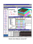
library. You should see a window as shown in Figure 1:
Figure 1: Library ExplorerWindow
When you open the library for the first time, Electric may ask you whether or not to use
the new settings (the one with the library) or keep the old settings. You want to use the
NEW settings (i.e., the settings that are in this library). If you get this message, it will
only be when you open the library for the first time.
There is already a cell named nand2 in the library with an {ic} (icon) view, you will
create additional views for this cell. To create a new view, choose Cell • New Cell to
bring up the Cell dialog, and enter nand2 as the cell name and schematic as the view. A
new editing window will appear with the title lab1_xx:nand2{sch} indicating the
library, cell name, and view. You can use the ‘+’ by each cell to expand a cell to see the
available views; double clicking on a view will open a window for that view.
Electric defines various components for schematics and layout. To see the available
components for schematic creation, clock on the components tab in the library window,
and select schematic from the choice list if it is not already selected. You will see a
component window as seen in Figure 2; this component list contains basic circuit
elements such as transistors, resistors, capacitors, and power and ground.
3
Jan 2010/V0.6
Figure 2: Library Component Window
Your goal is to draw a gate like the one shown in Figure 3 (your transistor sizes will be
different however). Choose Window • Toggle Grid to turn on a grid to help you align
objects. Left-click on an nMOS transistor symbol in the components menu on the left
side of the screen. Left-click on your schematic window to drop the transistor into your
layout. Repeat until you have two nMOS transistors, two pMOS transistors, the circular
power symbol, and the triangular ground symbol arranged on the page. You may move
the objects around by left-clicking and dragging. The transistors default to a width/length
value of 2/2. Double-click on the pMOS transistor and change its width to the value
specified in Table 1. Recall that nMOS transistors are roughly twice as strong as pMOS
transistors. So a single nMOS transistor would only have to be half as wide as the pMOS
transistor. However, because the nMOS transistors are in series, they should also be the
same width as the PMOS in this particular case.
Table 1 Transistor Width
Transistor Width
nMOS: 10+ last digit of MSU Net ID,
pMOS: 10+ last digit of MSU Net ID
4
Jan 2010/V0.6
Figure 3: nand2{sch}
Now, make the connections. Left-click on a port such as the gate, source, or drain of a
transistor. Right-click on another port to create a wire connecting the ports. Continue
until all the blue wiring is completed.
Finally, you will need to provide exports defining the ports (inputs and outputs) of the
cell. Left click on the end of a wire where you need to create the export for input a. You
should see a small square box highlighted at the end of the wire. If the entire wire is
highlighted, you clicked on the middle of the wire instead of the end, so try again. Once
you have selected the end of the wire, choose Export • Create Export. Give your export
the name a. Give it the characteristic Input. Repeat with the other input b. Export y as an
Output. Select the wire between the nmos transistors by left-clicking on it, then examine
its properties by using Edit • Properties • Object Properties (ctrl+I). Change the name of
this internal net to c ; the labels of internal nets are only displayed if you explicitly
change the name. We are doing this so that this net can be viewed in the simulator later.
5
Jan 2010/V0.6
Use File • Save (Ctrl-s) to save your library. Get into the habit of saving often to guard
against software crashes; you should also create copies of your library. Also, learn the
keyboard shortcuts for the commands you use frequently.
4. Switch-Level Simulation
Our next step is to simulate the schematic to ensure it is correct. Electric has two built-in
switch-level simulators: IRSIM and ALS. ALS is buggy, so we will use IRSIM. IRSIM
treats transistors as switches that may be ON or OFF; it also understands resistance and
capacitance based on transistor sizes and crudely estimates switching delays.
First select File • Preferences; then open the Tools • Simulators options panel. Ensure
that the parameter file for IRSIM is specified as scmos0.3.prm; this contains resistance
and capacitance data for the technology we are using. Also select the RC model for
simulation. Start the simulation by selecting Tool • Simulation (Built-in) • IRSIM :
Simulate Current Cell. A waveform window will appear listing each of the nets in your
design. If you created your exports properly, you will see nets for a, b, and y, as well as
the internal net c, as shown in Figure 4.
Figure 4: Simulation of nand2{sch}, all inputs low
6
Jan 2010/V0.6
The simulator has two vertical white dashed-line cursors named main (long dashes) and
ext (short dashes). The main cursor is used to create stimulus. Click and drag the cursor
near the left edge (to time 0 ns as indicated by the display). Click on the a input in the
simulation window and press V to drive the input high (can also use the menu command
Tool • Simulation (Built-in) • Set Signal High at Main Time). Drag the main cursor to
some later time, and then press G to drive the a input low (can also use the menu
command Tool • Simulation (Built-in) • Set Signal Low at Main Time). Modify both the
a and b input stimului to match that of Figure 5. Check that the y output matches the
behavior you would expect for a NAND2 gate as shown in Figure 5 (the simulator runs
when you modify the stimulus). If it does not, fix the bug in your schematic and
resimulate. You can save stimuli to an external file via the Tool • Simulation (Built-in) •
Save Stimuli to Disk... command, and then reload it later with the Restore Stimuli from
Disk... command.
Figure 5: Simulation of nand2{sch}, with stimuli
Use the Window • Zoom In (Ctrl+7), Zoom Out (Ctrl+0), Pan Left (Ctrl+4), Pan Right
(Ctrl+6) to examine the a input transition and the subsequent y output transition until you
can see the delay between these events. Drag the main cursor to the a input transition and
the ext cursor to the y output transition to measure the delta time between these two
events (use the center button to make the main/ext cursors visible if they are off screen).
7
Jan 2010/V0.6
You will find that unloaded gate delays are under 100 ps. Gate delay depends on the
capacitance being driven, so attaching a realistic load will slow the gate.
Use the Windows • Adjust Position • Tile Vertically command to arrange the windows
so that you can see both the simulation window and your schematic at the same time as
shown in Figure 6. Watch the color-coding of the wires in the schematic change as you
drag the primary cursor back and forth. On the schematic, green indicates high, blue
indicates low, and black indicates x, an illegal value. When a signal is selected in the
waveform window, the corresponding net will be highlighted on the schematic. Similarly,
when a net is selected in the schematic then its waveform representation will be
highlighted. Watching the voltage levels change on the schematic is helpful for
debugging problems. Study your simulation and determine why the node between the two
nMOS transistors behaves as it does. A thick purple bar means that the state is floating,
undefined, or could not be made into a definite logic level.
Figure 6: nand2{sch} and IRSIM Simulation side-by-side
Make a habit of simulating each cell after you draw it so you catch errors while the
design is fresh in your mind.
You can use Tool • Print command to print the contents of a window, or better yet, just
do a screen capture of a window for insertion into a document or for printing.
IRSIM Command Files
Instead of creating stimulus graphically, it is much easier to create a text command file
that specifies the stimulus. The following is a simple command file for the nand2
schematic called nand2.cmd:
8
Jan 2010/V0.6
| set stepsize to 2 ns
stepsize 2ns
| a, b both low
l a b
| simulate for 1 stepsize
s
h a
s
h b
s
l a
s
l b
s
The command Restore Stimuli from Disk... command can be used to read this command
file and execute it within IRSIM. The ‘|’ (pipe symbol) is the comment symbol in IRSIM
and must start in column 1.
5. Layout
Now that you have a schematic simulating correctly, it is time to draw the layout. Choose
Cell • New Cell and enter nand2 as the cell name and layout as the view. We will be
targeting the AMI 0.5 μm process but using MOSIS submicron scalable rules so we could
easily adapt to the AMI 1.5 μm process or others. We will use the mocmos technology
(MOSIS CMOS technology), which is the default technology for the library you have
opened. To check that we are using this technology, use File • Project Settings to open
the project settings panel, then select Technology and verify that both the startup and
layout technology is set to mocmos as shown in Figure 7. Also verify that the Submicron
Rules radio button is selected, three metal layers are selected, and “Alternate Active and
Poly contact rules” are checked. The submicron rules are documented on the MOSIS
web page. Alternate Active and Poly contact rules are an older, cleaner set of design
rules that don’t involve half-lambda dimensions.
9
Jan 2010/V0.6
Figure 7: Project Setings/Technology
Left-clicking on the other Settings choices will show other parameters for this
technology, i.e, the Scale choice sets the Lambda 1 value for this technology; verify that
the scale is set to 300 nm (nanometers).
Finally, use File• Preferences to open the preferences window, then use General • Arcs
and set the default width for Metal-1 to 4 and for Metal-2 to 4 for convenience of layout.
Your goal is to draw a layout like the one shown in Figure 8. It is important to choose a
consistent layout style so that various cells can “snap together.” In this project’s style,
power and ground run horizontally in metal2 at the top and bottom of the cell,
respectively. The spacing between power and ground is 80λ center to center. No other
metal2 is used in the cell, allowing the designer to connect cells with metal 2 over the top
later on. nMOS transistors occupy the bottom half of the cell and pMOS transistors
occupy the top half. Each cell has at least one well and substrate contact. Inputs and
outputs are given metal1 ports within the cell.
You may find it convenient to have another sample of layout visible on the screen while
you draw your gate. Use the Cell • Place Cell Instance command and select inv{lay}, then
1
Lambda is normally defined as half of the minimum drawn gate length. Therefore, the minimum drawn
gate length (polysilicon width) is 0.6 μm even though the vendor describes the process is 0.5 μm.
10
Jan 2010/V0.6
click to drop this inverter in the layout window. Select the inverter and use the Cell •
Expand Cell Instances • All the way command to view the contents of the inverter. Study
the inverter until you understand what each piece represents.
You will probably find it helpful to turn on the grid using the Windows • Toggle Grid
command. The grid defaults to small dots every lambda and large dots every 10λ. You
can change this with the Windows • Grid Options command. Also by default, objects
snap to a 1-λ grid. This can be changed by using Windows • Alignment Options. You
can also move objects around with the arrow keys on the keyboard. Pressing the h or f
keys cause the arrows to move objects by a half or full lambda, respectively. You will
avoid messy problems by keeping your layout on a lambda grid as much as possible.
Inevitably, though, you will create structures that are an odd number of lambda in width
and thus will have either centers or edges on a half-lambda boundary.
You can verify the 80λ center-to-center spacing of the Vdd/GND metal in the inverter
layout by using Window • Toggle Grid (ctrl+G) to turn on the grid. Zoom in on the cell
until you can tell by the grid spacing that metal 1 (blue) is 4 units wide, then select the
cell and move it until the metal features of the cell are aligned on the grid. Then use the
Toggle Measure Distance (M) command to turn on the measure cursor. Start at the center
of the ground rail (bottom, magenta rectangle), left-click to anchor the measure, then use
the Pan Up (Ctrl+8) command (or scroll bars) to pan up to the center of the VDD rail and
complete the measurement by left-clicking in the center of the rail. Use the ESC key to
terminate the measurement. You should have a vertical white measurement line with the
label ‘dx=0, dy=80’ labled near the center. This verifies the cell has an 80λ center to
center spacing of the Vdd/GND metal, which translates to a 80 * 0.3 μm = 24 μm cell
height
11
Jan 2010/V0.6
Figure 8: nand2{lay}
Start by drawing your nMOS transistors. You will notice a small black crosshairs on the
, this is the cell center or origin point (0,0). Make sure that no part of your
screen
layout covers this origin point at this time; when the layout is finished we will move the
cell center to the proper location. Draw your initial layout a good distance from this
origin point.
Recall that an nMOS transistor is formed when polysilicon crosses N-diffusion. Ndiffusion is represented in Electric as green diffusion surrounded by a dotted yellow Nselect layer all within a hashed black P-well background. This set of layers is
conveniently provided as a 3-terminal transistor node in Electric. Move the mouse to the
components menu on the left side of the screen. As you move the mouse over various
objects, the node name will appear on the status line next to the word NODE near the
bottom left corner of the screen. Left click on the N-Transistor, shown in Figure 9, and
click again in the layout window to drop the transistor in place. Use the Edit • Rotate • 90
Degrees Counterclockwise command to rotate the transistor so that the red polysilicon
gate is oriented vertically. There are two nMOS transistors in series in a 2-input NAND
12
Jan 2010/V0.6
gate, so we would like to make each wider to compensate. Double-click on the transistor.
In the node information dialog, adjust the width to the same width as what you have used
in your schematic.
Figure 9: nMOS transistor before and after rotation and sizing
We need two transistors in series, so copy and paste the transistor you have drawn or use
the Edit • Duplicate command. Drag the two transistors along side each other so they are
not quite touching as shown in Figure 10.
Figure 10: nMOS transistors side by side
Left click the diffusion (source/drain) of one of the transistors to highlight/select the
source/drain node, then and right click on the diffusion of the other transistor to connect
the two as shown in Figure 11. The white line shows that an arc now connects the nodes
of the two transistors. The concept of node/arc connection is quite important in Electric;
this is the way that Electric understands that these two components are actually connected
13
Jan 2010/V0.6
to each other. If you simply place the two transistors side by side without connecting
them, then Electric will not be able to correspond the arc/node connections in the
schematic with the arc/nodes connections in the layout, and also the design rule checker
will generate many errors from what looks to be correct layout. It is suggested that you
read the section in the Electric User’ Manual titled Basic Editing • Circuit Creation to
fully understand the difference between nodes and arcs, and how to connect them.
Figure 11: nMOS transistors with series connection
Then drag the two transistors until the polysilicon gates are 3λ apart, as shown in Figure
12.
14
Jan 2010/V0.6
Figure 12: nMOS transistors spaced 3λ apart
Electric has two design rule checker (DRC) tools for layout; incremental and
hierarchical (full). If the incremental DRC is turned on, then it is constantly running as
you generate layout. Because of the number of errors generated by the incremental DRC
and because we will be working with small layouts, it is suggested that you turn off the
incremental DRC. Selecting File • Preferences to open the preferences window, then
select Tools • DRC and ensure that the incremental DRC checkbox is not checked as
shown in Figure 13. Hierarchical (Full) DRC does a more complete job than incremental
DRC, and is fast on small layouts, so it is suggested that you always use Full DRC.
15
Jan 2010/V0.6
Figure 13: DRC Preferences
Full DRC is avaiable from the F5 hotkey or from Tool • DRC • Check Hierarchically
menu choice. To test Full DRC, try dragging one of the transistors until its gate is only 2λ
from the other. Hit F5 and observ the DRC error message(s) printed to the message
window. In the Explorer window, you can open the Errors/Layout DRC (full)[current]
view to see a list of errors; double clicking on one them will highlight the error in the cell
as shown in Figure 14. DRC error listings are placed in folders under the Explorer tab;
delete the folder to delete the error listings. You can also use the > key to sequence
through and highlight errors. It is suggested that you check your layout often for errors by
using the F5 hotkey to perform Full DRC.
.
16
Jan 2010/V0.6
Figure 14: DRC Report
Move the transistors back to a 3λ spacing, delete the DRC folder, and use Full DRC
(hotkey F5) to ensure that the layout contains no errors at this point
An Aside on Design Rules
The definitive design rules are available on the MOSIS web page. MOSIS
is a service that collects small orders for designs and combines them into
an order large enough to interest a semiconductor manufacturing facility.
For best density, one could optimize for a particular fabrication process
and design in units of microns rather than lambda. However, the layout
would require redrawing when ported to a different process because the
design rules and feature size will have changed. MOSIS has developed a
set of Scalable CMOS design rules that are sufficiently conservative to
work for virtually all processes. The original rules, SCMOS, apply to older
processes. We will be using the SUBM submicron rules that are even more
conservative and suffice for more advanced processes. They are adequate
17
Jan 2010/V0.6
for both the AMI 0.5 and 1.5 micron processes. Finally, the DEEP deep
submicron rules are slightly more conservative and are necessary for best
performance in the 0.25 μm and below processes. For historical reasons,
all three sets of rules are selected in Electric by choosing the scmossub
process, then using the Technology Options dialog. Tables 3 and 4 on the
MOSIS web page list the differences between these design rules.
http://www.mosis.org/Technical/Designrules/scmos/scmos-main.html
We will be fabricating using the SCNE technology code defined in Table
5 of the web page. SCNE means Scalable CMOS with N-wells and an
Electrode layer, i.e. polysilcon 2. Click on each of the layers in the table to
see the design rules. For example, the Metal1 rules are shown in Figure 15
below. We will follow the SUBM rule set, requiring metal width and
spacing of 3λ.
SCMOS Layout Rules - Metal1
Rule
7.1
7.2
7.3
7.4
Description
SCMOS
3
2
1
Minimum width
Minimum spacing
Minimum overlap of any contact
Minimum spacing when either metal
4
line is wider than 10 lambda
Lambda
SUBM
3
3
1
6
DEEP
3
3
1
6
Figure 15: SCMOS Metal1 Rules
Next we will create the contacts from the N-diffusion to metal1. Diffusion is also refered
to as active area. Drop a square of Metal-1-N-Active-Contact in the layout window and
double-click to change the properties to a Y size to match your transistor width. Move the
contact near the end of the transistor stack and connect it as shown in Figure 16 (left click
on the contact, the right click on the diffusion transistor node).
18
Jan 2010/V0.6
Figure 16: nAct contact to N-transistor
Repeat this process for the second contact that is required for the other end of the series
stack of nMOS transistors. Then move the contacts nearer the transistors until there is
only a gap of 1λ between the metal and polysilicon. Use the design rule checker to ensure
you are as close as possible but no closer. Using similar steps, draw two pMOS
transistors in parallel and create contacts from the P-diffusion to metal1. At this point,
your layout should look something like Figure 17:
Figure 17: Contacted transistors for nand2 layout
To make it easier to follow the cell template, align the bottom of the N-transistors of the
nand2 layout with the bottom of the N-transistors of the inverter layout, and the top of the
P-transistors of the nand2 with the top of the P-transistors of the inverter as shown in
Figure 18. We will eventually delete the inverter layout, but it is handy to keep around as
19
Jan 2010/V0.6
a reference for now. Observe that wide transistors grow towards the center of the cell
template.
Figure 18: inv and nand2 layout side by side
Draw wires to connect the polysilicon gates, forming inputs a and b. To draw a
polysilicon wire, left-click at the end of a poly gate, then right click on the end of the
destination poly gate, to form the connection as shown in Figure 19. Repeat the process
for the other gate connection, referring to the layout of Figure 8 (to create a jog, right
20
Jan 2010/V0.6
click in the empty space to create each wire segment).We will place the metal2 contacts
for the a and b inputs at a later time.
Figure 19:Poly gate connection
To create the metal1 output node y, move the mouse over the center P-active contact until
the contact is highlighted (not the transistor), then left click to select. Then right click
somewhere below the P-transistor strip as shown in Figure 20 to create a vertical metal1
wire.
21
Jan 2010/V0.6
Figure 20:Vertical Metal1 Wire
Then right-click on the end of the wire, and drag to create a vertical wire to the NMOS
transistor strip. When you reach the N-transistor strip, you will note that the N-transistor
may be highlighted; if you release the right button you may create a contact to the
diffusion area (use Edit • Undo to remove if this occurs). Use the space bar to cycle
through connection points until no connection points are highlighted, then release the
right mouse button. This is will terminate the metal wire without connecting it to
anything as shown in Figure 21.
22
Jan 2010/V0.6
Figure 21:Metal Wire
Left click on the end of the metal wire to select the end node, then right-click-drag over
the contact; use the space bar to cycle through connection targets until the contact is
highlighted, then release the mouse button. This should complete the metal wire
connection as shown in Figure 22.
23
Jan 2010/V0.6
Figure 22:Completed Metal Wire
Then add metal2 power and ground lines. You can add a line by selecting a pin such as
metal-2-pin from the Misc. component palette (do not use the Pure palette) then rightclicking nearby to draw the line. Use the grid to ensure they are 80λ apart from the center
of each line. This is the same spacing as the power/ground lines of the inverter. A metal1metal2-contact, also known as a via, is required to connect the metal1 to the metal2 lines.
Left-click on an active contact. Right-click on the ground line. Electric will
24
Jan 2010/V0.6
automatically create the necessary via for you while making the connection. Complete
the other connections to power and ground. Let power and ground extend 2 lambda
beyond the contents of the cell (excluding wells) on either side so that cells may “snap
together” with their contents separated by 4λ so design rules are satisfied (follow the
style of the inverter layout).
Recall that well contacts are required to keep the diodes between the wells and
source/drain diffusion reverse biased. We will place an N-well contact and a P-well
contact in each cell. It is often easiest to drop the Metal1-N-Well-Con near the desired
destination (near VDD,), then right click on the power line to create the via (Figure 23).
Then drag the contact until it overlaps the via to form a stack of N+ diffusion, the
diffusion to metal1 contact, metal1, the metal1-metal2 via, and metal2 (Figure 24).
Figure 23:N-well contact placed above Vdd and connected to Metal2 VDD
Figure 24:N-well contact dragged under the Metal2 Via
Observe that the N-well (dotted black) does not extend evenly around the cell; the small
segment that juts out from the VDD and substrate contact will cause a DRC error at this
point; this will be fixed later.
Repeat this process to place the P-well contacts.
25
Jan 2010/V0.6
In our datapath design style, we will be connecting gates with horizontal metal2 lines.
Metal2 cannot connect directly to the polysilicon gates. Therefore, we will add contacts
from the polysilicon gate inputs to metal1 to facilitate connections later in our design.
Place a metal-1-polysilicon-1-contact near the left polysilicon gate. Connect it to the
polysilicon gate and drag it near the gate. You will find a 3λ separation requirement from
the metal1 in the contact to the metal forming the output y. Add a short strip of metal1
near the contact to give yourself a landing pad for a via later in the design. You may find
Electric wants to draw your strip from the contact in polysilicon rather than metal1. To
tell Electric explicitly which layer you want, move the mouse over the palette until it is
over the blue Metal-1 arc square and click. Then draw your wire.
Electric is agnostic about the polarity of well and substrate; it generates both n- and pwell layers. In our process that has a p-substrate already, the p-well, indicated by black
slanting lines, is actually not needed but is still checked by the MOSIS SUBM rules (so
any rule violations of p-well can be ignored, but it is a good idea to correct these
violations so that they do not mask other errors). The n-well, indicated by small black
dots, will define the well on the chip. Electric only generates enough well to surround the
n and p diffusion regions of the chip. It is a good idea to create rectangles of well to
entirely cover each cell so that when you abut multiple cells you don’t end up with
awkward gaps between wells that cause design rule errors. To do this for the n-well
(covers the p-transistors), left click in the top of the Pure component menu to bring up a
list of layers, then select N-well-node and place this rectangle above the p-transistors.
While it is still selected (highlighted), use ctrl+I (Edit • Properties • Object Properties)
and set the X,Y values to form a square that will complete cover the P-transistors in the
same manner as the inverter. If the n-well square becomes unselected, you will have
trouble reselecting it as a pure layer is marked as ‘hard-to-select’ because often you want
to move other objects around with moving pure layer objects. To re-select the object,
button in the upper menu; you will now be able to
click on the Toggle-special-select
select the n-well square. After you have filled in the n-well, do the same for the p-well for
consistency purposes
Create exports for the cell. When you use the cell in another design, the exports define
the locations that you can connect to the cell. Click near the end of the short metal1 input
lines that you just drew on the left gate. You will see a small white box highlighted,
corresponding to the pin at the end of the cell. If you accidentally selected the entire line
instead, click elsewhere in space to deselect the line, then try again to find the pin. You
may also try holding the ctrl key while clicking to cycle through selections. Add an input
export called a. Repeat for input b. Export output y from the metal line connecting the
nMOS and pMOS transistors. You may have to place an extra pin and connect it to the
output line to give yourself a pin to export as y. Also export vdd and gnd from the metal
2 lines; these should be of type power and ground, respectively. Electric recognizes vdd
and gnd as special names, so be sure to use these names.
The last task is to position your cell layout at the correct origin, or cell center point.
Having a cell center avoids some off-grid weirdness in Electric. The cell center point is a
26
Jan 2010/V0.6
small black crosshair
.as mentioned previously. Save your layout, then open the
layout for the inverter and note that the cell center is located in the center of the gnd rail,
2λ in from the left edge. The cell center can be selected using the Toggle-special-select
button. Using cell centers on all your icons and layout cells will avoid nasty offgrid errors later in your work. Select the cell center object, and move it to its proper
place on your layout (the same location as in the inverter layout).
Your design should now resemble Figure 8 and should pass DRC. When you are done
drawing the nand2 layout, click on the inverter and press delete to remove it from the
cell. Save the library.
Electric has a fun feature to show a 3D rendition of your layout. Use the Windows • 3D
Display • View in 3 Dimensions command. Click and drag with the mouse to rotate the
layout. You will see the layer stack from diffusion on the bottom through polysilicon,
metal1 and metal2. Vias are shown in white and contacts from metal1 to poly or diffusion
in black. Does the 3-D visualization match your mental picture of the layout? When you
are done, use Windows • 2D Display • View in 2 Dimensions to restore normal viewing.
6. Layout Verification
Layout verification involves more checks than schematic verification. The checks include
Design Rule Checks (DRC), Electrical Rule Checks (ERC), Network Consistency
Checking (NCC), and simulation.
You will likely find yourself invoking these menu options often and may wish to give
yourself keyboard shortcuts. To set key bindings, open the preferences window with File
• Preferences, then open the General folder and left click on Key Bindings. In the righthand pane, open the folder Tool, and you will see subfolders for Tool choices. To bind
the NCC tool to F3, open the Tool|NCC folder, then left click on Tool|NCC|Schematic
and layout Views of Cell in Current Window. Then click on the Add button in the lower
half of the window to set a key binding. Another shortcut you may want to consider is F4
for Tool|ERC|Check Wells.
First, be sure the design satisfies the layout design rules by running a hierarchical DRC.
This checks the layout and any cells it might incorporate; in this case the nand2 is a leaf
cell and has no subcells. Correct any DRC violations that might remain.
Next, run Tool • ERC • Check Wells. This check ensures that every N-well has a contact
to VDD and every P-well has a contact to GND reasonably close by. A common cause of
ERC violations is to not export power and ground or to give them the wrong names or the
wrong type of export.
Next, simulate the layout using IRSIM. Apply a complete set of stimulus to the two
inputs to convince yourself that the gate is working correctly. You can also use Tool •
27
Comment [rbr1]: There seem to be a lot of
differences here between the C-Electric and JavaElectric in terms of what is reported for both ERC
and NCC. In the original document, you mention
that ERC reports the number of transistors and the
max distance from any part of a layout to a well or
substrate contact, but I don’t get those reports with
Java-Electric and I can’t find any options for the
DRC to control the verbosity of its output.
NCC has different reports as well since the tools
have changed between C-electric and Java-Electric,
but it has a verbosity option that I mention in the
document.
The new NCC does not catch different ordering of
series transistors, this is discussed in the new NCC
documentation.
Jan 2010/V0.6
Simulation (built-in) • Restore Stimuli from Disk to load your previous stimulus,
assuming that you have saved it to disk previously.
Electric includes a powerful tool called a network consistency checker that checks that
the schematic and layout are equivalent. This is especially valuable when your design is
too complex to verify completely through simulation. The checker relies upon graph
theory algorithms. If your layout and schematic match, you have much greater confidence
that a bug hasn’t crept into your design. Unfortunately, if the two don’t match, the tool
becomes very confused and provides few hints. Also, NCC uses a rather complex
algorithm and has been the source of quite a few bugs in Electric, so don’t trust it blindly.
To use NCC, first open the preferences window (File • Preferences), then open the Tools
folder and left click on NCC to display its options. Ensure that ‘Check Transistor Sizes’
and ‘Hierarchical Comparison’ are checked as shown in Figure 25.
Figure 25:NCC Options
Then, ensure that the nand2{lay} cell is open is open, and run Tool • NCC • Schematic
and layout Views of Cell in Current Window. You should receive the report as shown
below:
28
Jan 2010/V0.6
Hierarchical NCC every cell in the design: cell 'nand2{sch}' cell 'nand2{lay}'
Comparing: lab1_rbr:nand2{sch} with: lab1_rbr:nand2{lay}
exports match, topologies match, sizes match in 0.0 seconds.
Summary for all cells: exports match, topologies match, sizes match
To see an example of a schematic/layout mismatch, open nand2{sch} and change one of
the transistor sizes and rerun NCC. You will then get are report for the mismatched
transistor sizes. In the NCC preferences, you can get more information about the
extracted layout by setting the Reporting Progress value to a number higher than 0.
One thing that NCC does not check is the series ordering of transistors in your layout
versus your layout; you can have a different series ordering between layout and
schematic and NCC reports that the topology matches; this appears to have been done for
execution speed reasons.
If your design is not equivalent in any nontrivial way, NCC will likely mark too much
mismatching to be useful. Identifying the error is part of the art of using NCC. If
possible, simulate both the layout and schematic carefully to eliminate obvious errors.
Carefully examine your design by hand to look for errors. There is a good help section on
NCC, read it for more information.
7. Hierarchical Design
Now that you have a 2-input NAND gate, you can use it and an inverter to construct a 2input AND gate. Such hierarchical design is very important in the design of complex
systems. You have found that the layout of an individual cell can be quite time
consuming. It is very helpful to reuse cells wherever possible to avoid unnecessary
drawing. Moreover, hierarchical design makes fixing errors much easier. For example, if
you had a chip with a thousand nand gates and made an error in the nand design, you
would prefer to only have to fix one nand cell so that all thousand instances of the nand
inherit the correction than to need to fix each nand individually.
Each schematic has a corresponding symbol, called an icon, used to represent the cell in a
higher-level schematic. For example, open the inv{sch} and inv{ic} to see the inverter
schematic and icon provided. You have also been provided an icon for your 2-input
NAND gate. The remaining instructions can be referenced if you find the need to create
an icon for a cell in the future. YOU DO NOT HAVE TO CREATE A NEW ICON FOR
YOUR NAND2, just use the one that is provided.
Create a new schematic called and2. Use Edit • New Cell Instance to create
(“instantiate”) the nand2{ic} and an inv{ic} (the inverter already exists in the library).
Wire the two together and create exports on inputs a and b and output y. Double-click on
the wire between the two gates and give it a name like yb so you know what you are
looking at in simulation. It is good practice to label every net in a design if practical.
When you are done, your and2 schematic should look like Figure 29. If the line between
29
Jan 2010/V0.6
the gates is black rather than blue, you neglected to return to the schematic, analog
technology and were still drawing using the artwork palette.
Figure 26: and2{sch}
Simulate your and2 gate to ensure it works. You can use the Tools • Simulation • Down
Hierarchy command to descend into the nand gate and see its internal node. In the
schematic editor, you can double-click on each gate and assign it a name to help
differentiate cells when you simulate.
Next, create a new layout called and2. Change the technology to mocmos. Instantiate the
nand2{lay} and inv{lay} layouts (the inverter layout already exists in the library, use it
without changes). ALWAYS use the New Cell Instance to create layout from preexisting
cells. NEVER build a cell by cutting and pasting entire existing cells. If you do, then
make a correction to the original cell, your correction will not propagate to the new
layout. However, this does mean that you will need to make all the connections to
existing ports in your instantiated cells.
Initially the layouts appear as black boxes with ports. Select both and use the Cell •
Expand Cell Instances • All the Way command to view the contents of each layout. Wire
together power and ground. Move the cells together as closely as possible without
violating design rules. You may need to place large blobs of pure layer nodes over the nwell and p-well to avoid introducing well-related errors from notches in the wells.
Connect the output of the nand2 to the input of the inv using metal1. Remember that
connections may only occur between the ports of the two cells. Also connect the power
and ground lines of the cells using metal2. Export the two inputs, the output, and power
and ground. The final and gate should resemble Figure 30. Run DRC, ERC, and
simulation to verify your design.
30
Jan 2010/V0.6
Figure 27: and2{lay}
Finally, do a network compare. NCC has three modes in the NCC Options: Expand
hierarchy, Recurse through hierarchy, and neither. Expand hierarchy smashes your entire
design into one giant netlist for its internal comparison. Recurse through hierarchy checks
each subcell on each hierarchical level. NCC is a relatively new feature that has received
many bug fixes, so it is wise to try both Expand hexarchy and Recurse through hierarchy
to catch any problems that one mode misses. Do not check both Recurse through
hierarchy and Expand hierarchy, as it will give meaningless results. In each case, be sure
to check Check export names, Check component sizes, and Ignore Power and Ground.
Do not set any individual cell overrides. After you check a cell, Electric marks it as clean
and thus not in need of rechecking.
If NCC reports a problem, check that your inputs are in the correct order. If a and b are
reversed between the layout and schematic, you will get an error that nodes are wired
differently. If VDD or GND are not exported, you will also get many errors and your
simulations will produce invalid levels. Tracking NCC mismatches is very difficult, so
you are best off ensuring your design is correct by means of careful drawing and
simulation rather than drawing sloppily and hoping to catch problems with the checker.
Keep a list in your notebook of any design errors you made that caused NCC problems
and note the symptoms reported by NCC. In the future, you can use this experience to
help you find problems in complicated designs more quickly.
Now that your and2 gate is complete, use the Info • Check and Repair Libraries
command to look for any inconsistencies in your library. You shouldn’t expect any, but
Electric has been known to do strange things from time to time, especially in the hands of
novice users. Therefore, you may wish to check your library every few hours.
31
Jan 2010/V0.6
8. NOR / OR Gate Design
Your MIPS processor supports the OR instruction as well as the AND instruction.
Therefore, you will need to create a 2-input NOR and a 2-input OR gate. Call these nor2
and or2. The nMOS, pMOS transistors should be the widths specified in Table 2. For
each gate, create schematic and layout cells following the same steps you used with the
nand2 / and2. Be sure to export the inputs, output, power, and ground. Simulate each
to ensure correct operation. Run DRC, ERC, and NCC to check each layout. Be sure to
save your work frequently. It is wise to keep a backup of your work from time to time in
case your library becomes corrupted.
Table 2 Transistor Widths for NOR/OR Gates
Last Digit of MSU Net ID
0,1,2
3,4,5
6,7,8,9
Transistor Sizes
nMOS: 4, pMOS:16
nMOS:5, pMOS: 20
nMOS:6, pMOS: 24
9. What to Turn In
Follow the directions on the class website for submitting the files listed below. It is
expected that all layouts pass DRC, NCC and simulate in IRSIM correctly.
Part A submission:
1. Your Electric library file (.elib) that contains all of your cells (nand2{sch}{lay}
and2{sch}{lay})
2. An IRSIM command file named and2.cmd that exercises your and2{lay} cell.
Part B submission:
3. Your Electric library file (.elib) that contains all of your cells (nor2{sch}{lay}
or2{sch}{lay})
4. An IRSIM command file named or2.cmd that exercises your or2{lay} cell.
10. Changelog
November 2006: Modified for use with Java Electric (R. Reese/Mississippi State
University) and made other MSU-specific changes. Original author is D. Harris.
32
Jan 2010/V0.6
11. Creating an ICON
These instructions can be referenced if you need to create an ICON view for a cell.
When creating an icon, it is a good idea to keep everything aligned to the 1-λ grid, this
will make connecting icons simpler and cleaner when you need it for another cell.
Open your nand2{sch} and choose View • Make Icon. Electric will create a generic icon
based on the exports looking something like Figure 28. It will drop the icon in the
schematic for handy reference; drag the icon away from the transistors so it leaves the
schematic readable.
Figure 28: nand2{ic} from Make Icon
A schematic is easier to read when familiar icons are used instead of generic boxes.
Modify the icon to look like Figure 27. Pay attention to the dimensions of the icon; the
overall design will look more readable if icons are of consistent sizes.
Figure 29: nand2{ic} final version
Click on the icon and choose Cells • Down Hierarchy to drop in to the icon. The
technology will automatically change to artwork. A palette will appear with various
shapes. Delete the generic red box but leave the input and output lines. Turn on the grid.
If there is not already a cell center in the cell, place a cell center in the center of the icon
using the Edit • New Special Object • Cell Center command. Drag the cell center where
you want it.
33
Jan 2010/V0.6
The body of the NAND is formed from an open C-shaped polygon, a semicircle, and a
small circle. To form the semicircle, place an unfilled circle. Double-click to change its
size to 6x6 and to span only 180 degrees of the circle. Use the rotate commands under the
Edit menu to rotate the semicircle into place. Place another circle and adjust its size to
1x1. You will need to change the alignment options under the Windows menu to 0.5 to
move the circle into place, then set alignment back to 1. Alternatively, you can press h
and use the arrow keys to move objects by ½ grid increments, then press f to return to full
grid movement.
The opened-polygon shown in Figure 28 can be used to form the C-shaped body. Drop an
opened-polygon object. Select it and choose Edit • Special Function • Outline Edit to
enter outline edit mode. In this mode, you can use the left button to select and move
points and the right button to create points. You should be able to form the shape with
four clicks of the right button to define the four vertices. Outline edit mode is not entirely
intuitive at first, but you will master it with practice. Choose Edit • Special Function •
Exit Outline Edit when you are done. If your shape is incorrect, delete it, drop another
opened-polygon, and try again.
Figure 30: Opened-Polygon
Electric is finicky about moving the lines with inputs or outputs. If you left-click and drag
to select the line along with the input, everything moves as expected. If you try to move
only the export name, it won’t move as you might expect. Therefore, make a habit of
moving both the line and export simultaneously when editing icons. Note that the line is
just an open-polygon and can be shortened if desired by entering Outline Edit mode.
Use the Text item in the artwork palette to place a label “nand2” in the center of the icon.
12. IRSIM Commands
This is a historical tutorial on IRSIM taken from the following source:
http://www.stanford.edu/class/ee272/doc/faq/irsim/irsim_tut.txt .
IRSIM functionality has been replicated within Java Electric. This tutorial presented here
as a command reference.
The IRSIM Tutorial
version 1.1
(last modified by Williams, 11-apr-95)
This is a simple tutorial on irsim.
It is not meant to
34
Jan 2010/V0.6
replace the irsim manual which contains much more
information.
1.0
Which computers can use IRSIM
At the time of this writing, irsim is only supported on
the Sparcstations (elaines). For some reason,
remote login from an IBM (airrs) to an elaine does not work
at all. You can run irsim, but it will not work correctly.
Save yourself some grief. Don't bother using the IBM's.
Remote login from a DECstation (adelbert) does work.
However, you cannot set up your analyzer window from a .cmd
file. You must do it within irsim. More on .cmd files and
analyzer windows soon.
On an appropriate computer, you can just say "irsim" or
explictly "~cad/bin/irsim"
2.0
Creating a .sim file
Irsim files are just text files that contain information
about a circuit. They have the extension .sim. The first
time you use irsim, you will probably have to create the .sim
file yourself using your favorite text editor. Later you'll
create it from a layout that you do in Magic.
Below is a CMOS circuit to implement ~a~b + ~c where ~a
means the inverse of a.
Vdd
___________
___|
|
||
|
a ---o||
|
||___
|
|
|___
| n1
||
|
||o--- c
___|
___||
||
|
b ---o||
|
||___
|----------- out
|___________|
___|
|___
||
||
a ----||
||---- b
||___
___||
|___________|
|
___| n2
||
c ----||
||___
|
_|_ Gnd
\ /
V
35
Jan 2010/V0.6
The first step in creating a .sim file for this circuit
is to label all the nodes. Label power Vdd and ground Gnd.
Irsim is not case sensitive so vdd and gnd will work also.
You can label the other nodes anyway you want. Use any
method you wish. For the circuit above, the inputs are
labeled a, b, c and the output node is labeled out. Other
internal nodes are labeled n1 and n2. When using irsim, it
is helpful to have the labeled circuit schematic available so
that you know the names of the nodes that you want to probe.
The .sim file for the above circuit is shown below.
|
units: 50
tech: scmos
p
p
p
a
b
c
vdd
n1
vdd
n1
out
out
2
2
2
4
4
4
n
n
n
a
b
c
out
out
n2
n2
n2
gnd
2
2
2
4
4
4
The first line is a comment. Any line that begins with
the vertical bar '|' is a comment. Everybody knows the
purpose of comments I hope. This first line says that the
technology used is scalable cmos.
Transistors are specified as follows:
type
g
s
d
l
w
where type is p for pmos and n for nmos. The g refers to the
name of the gate terminal. Similarly, s refers to the name
of the source terminal and d refers to the drain. This is
why you need a labeled circuit schematic to create a .sim
file by hand. It is important that you get the connections
correct. The l is the length of the transistor and the w is
the width, both in microns.
The first transistor specified in the example
above is the top-left pmos transistor in the corresponding
schematic. Study the rest of the irsim file and the circuit.
It is easy to see how the two match. You can also enter in
resistors and capacitors. See the irsim manual for the
proper format to create these elements. Considering just
transistors, you are now ready to run irsim.
3.0
Starting IRSIM
At the unix prompt type
irsim /usr/class/ee/lib/scmos50.prm myfile.sim
scmos50.prm is the technology file and the .sim is any irsim
file. The explicit path to the prm is not required if your
CAD_HOME is set correctly to "/usr/class/ee/lib", which it will
36
Jan 2010/V0.6
be if you have run a good setup file.
For example, if your .sim file is named circuit.sim type:
source /usr/class/ee271/setup
irsim scmos50.prm circuit.sim
irsim will tell you how many transistors you have and then
display the irsim prompt shown below.
IRSIM>
3.1
Running IRSIM
You can enter in commands interactively or you can run a
script. Scripts are just the .cmd files and they contains
commands that are exactly what you would type in at the irsim
prompt.
Here is an example irsim session. The IRSIM> prompt precedes
commands that were entered interactively. Text preceded by
the vertical bar | is output from irsim. Instructional
comments will be preceded by //.
IRSIM> stepsize 50
//
//
//
//
//
//
The basic idea of irsim is that you tell it which nodes
to pull high, which nodes to pull low, which nodes to
tristate, and then you tell irsim to run the simulation
for a certain period of time. This period of time is the
stepsize. The above command tells irsim that the
stepsize is 50ns. The default stepsize = 100 nanoseconds.
IRSIM> w out c b a
//
//
//
//
//
//
The command 'w' tells irsim to watch the following nodes.
So the above command tells it to watch the nodes out, c,
b, and a. Irsim displays the nodes in the reverse order
in the above command. Therefore the output order will be
a b c out. This is just a matter of personal preference
though. Enter in the nodes in any order you like.
IRSIM> d
//
//
//
d displays all the nodes that are being watched.
You can also enter in something like 'd a b' which tells
irsim to only display nodes a and b
| a=X b=X c=X out=X
| time = 0.0ns
//
at time zero, the values of the nodes are all undefined
IRSIM> l a b c
//
The l command forces the nodes to a logic value of 0
37
Jan 2010/V0.6
//
The above command sets nodes a b and c to logic 0
IRSIM> s
//
//
//
s tells irsim to simulate for a certain period of time
previously defined by the stepsize command. The default
value is 100 ns, but we set it to 50ns above.
| a=0 b=0 c=0 out=1
| time = 50.0ns
//
//
//
//
Irsim displays the values of the nodes after each step
because of the previous d command. The current time is
also displayed. Note that time = 50 ns. This is
the current simulation time now.
IRSIM> h c
//
//
h sets the following nodes to a logic high value.
Therefore the above command sets node c to logic 1.
IRSIM> s
| a=0 b=0 c=1 out=1
| time = 100.0ns
//
step
IRSIM> h b
IRSIM> s
| a=0 b=1 c=1 out=0
| time = 150.0ns
IRSIM> path out
| critical path for last transition of out:
|
b -> 1 @ 100.0ns , node was an input
|
out -> 0 @ 100.1ns
(0.1ns)
//
//
//
//
//
//
The path command shows the critical path for the last
transition of a node.
The output shows that an input node 'b' changed to
logic 1 at time = 100 ns. The node 'out' then
transitioned low at time = 100.1 ns. Therefore it took
.1 ns to go from high to low for the given input changes.
//
//
You can look back at previous commands to verify that
this is indeed what happened.
//
//
//
//
//
//
//
//
Sometimes you may want to find out what the worst case
Tplh or Tphl is. The path command helps you find this
number. You do this by setting the circuit to some state
and then force inputs to change that will cause a
transition at the output. Some intelligence is required
to figure out what the worst state is and what
combination of input changes will cause the slowest
output transition.
38
Jan 2010/V0.6
//
//
//
//
If you have a long list of inputs, it can be tiresome to
keep using the l and h commands to set the logic
values. The 'vector' command lets you group inputs
together so that you can set them all quickly
IRSIM> vector in a b c
//
//
The above command tells irsim to group the nodes a b and
c into a vector called 'in'
IRSIM> set in 000
//
//
This command tells irsim to set the vector in to 000
Therefore, node a = 0, node b = 0, and node c = 0
//
//
//
//
The following commands demonstrate how you can create a
truth table using the vector 'in'. Note that you can do
this much faster this way than by using the commands
l and h.
IRSIM> s
| a=0 b=0 c=0 out=1
| time = 200.0ns
IRSIM> set in 001
IRSIM> s
| a=0 b=0 c=1 out=1
| time = 250.0ns
IRSIM> set in 010
IRSIM> s
| a=0 b=1 c=0 out=1
| time = 300.0ns
IRSIM> set in 011
IRSIM> s
| a=0 b=1 c=1 out=0
| time = 350.0ns
IRSIM> set in 100
IRSIM> s
| a=1 b=0 c=0 out=1
| time = 400.0ns
IRSIM> set in 101
IRSIM> s
| a=1 b=0 c=1 out=0
| time = 450.0ns
IRSIM> set in 110
IRSIM> s
| a=1 b=1 c=0 out=1
| time = 500.0ns
IRSIM> set in 111
IRSIM> s
| a=1 b=1 c=1 out=0
| time = 550.0ns
//
//
//
irsim has a built in graphical logic analyzer which
runs under X to let you view waveforms.
If you haven't set your DISPLAY variable
39
Jan 2010/V0.6
//
//
correctly before entering irsim, then you can use
the "Xdisplay" command within irsim to set it.
IRSIM> Xdisplay myelaine:0.0
//
The 'analyzer' command sets up the analyzer window
IRSIM> analyzer a b c out
//
//
This tells irsim to display the nodes a b c and out in
the analyzer window
3.2
Using the analyzer window
Go ahead and experiment with the analyzer window. It's
pretty easy to use. Here are some of the things that you can
do.
3.2.1.
Print the waveforms to a postscript file
Go to the 'print' menu and select 'file'. You will be asked
for a filename. Hitting return selects the filename shown in ().
Once you have the postscript file, you can print it out on
one of the network printers using lpr.
3.2.2.
Setting the width
3.2.2a.
You can set the width of the view from either the menus
or the slider on the bottom. From the menus, select 'window'
and then 'set width'. You will be asked to enter the width
in time steps. Use the 'move to' option under the 'window'
menu to move to the desired time.
You can also use the 'zoom' menu to zoom in and out.
3.2.2b.
The best way to get a feel for the slider on the bottom
is to play with it. Using the left mouse button expands the
view or shortens the view to the left depending on where you
click. Clicking using the right mouse button expands or shortens
the view to the right depending on where you click. You can
grab the slider with the middle button and move it around.
3.2.3.
Changing the order of the nodes
If you don't like the order that the nodes are
displayed, you can click inside the name with the left
mouse button, and drag it to a new place.
Play around with this to see how it works.
3.2.4.
Finding the time of an event
You can click inside the analyzer window where the waveforms
are to get a vertical line. The time where this vertical line
is is displayed above. This is useful if you want to find out
when a rising edge occurs. The resolution is best when you are
zoomed in.
40
Jan 2010/V0.6
//
//
//
//
You have seen the commands 'l' and 'h' to set nodes to
logic 0 or logic 1. The 'x' command will effectively
put a node into tristate. It does this by taking the
node off the input list.
//
The following is an example of using the x command
IRSIM> x bus
//
//
//
//
//
//
//
//
puts the node bus into tristate. An application of this is
simulating a register. Assume you have a one bit register
that is connected to a line called bus and is operated as
follows. To write a value in your register, you need to
drive the value onto the bus and then set a control line
write to high. To read the register, you first need to stop
driving the bus. Then set a control line read to high. The
irsim commands you need to issue are shown below.
IRSIM>
lines low
IRSIM> h
IRSIM> s
IRSIM> h
IRSIM> s
IRSIM> l
IRSIM> s
IRSIM> l
IRSIM>
IRSIM>
IRSIM>
IRSIM>
l read write
bus
//
write
//
step
//
write
//
//
bus
set
read
and
write
let's write a 1 into the register
write into the register
stop writing
//
//
// set bus to 0 so we can see the bus
transition from 0 to 1 when we read
the register
//
//
// stop driving the bus so we don't get
bus contention when we read the
register
//
// read the register;
0 to 1 transition
s
x bus
s
h read
you should see a
Irsim lets you keep a log of your commands and the outputs.
To start recording, type
IRSIM> logfile anyfilename
//
//
Anything that you see in irsim from now on will be
into the file 'anyfilename'
//
When you're done recording, type the following.
IRSIM> logfile
//
Quitting IRSIM
IRSIM> exit
3.3
control
Automation through .cmd files
41
Jan 2010/V0.6
Any irsim interactive command is valid. Use your favorite
text editor to create this file. An example is shown below
for the previous circuit.
stepsize 50
analyzer a b c out
vector in a b c
set in 000
s
set in 001
s
set in 010
s
set in 011
s
set in 100
s
set in 101
s
set in 110
s
set in 111
s
//
end of example;
do not type this comment in
This example runs through all the possible combinations of
inputs. The waveforms will be displayed in an analyzer
window. You can run a .cmd file from the command line or
within irsim. If the above file is called example.cmd, then
% irsim scmos50.prm circuit.sim -example.cmd
will run the command file on circuit.sim
To use a .cmd file within irsim, type 'example' as shown
below.
IRSIM> example
Note, you should not type 'example.cmd'.
is
IRSIM> @ example.cmd
but the previous way uses less keystrokes.
42
Another alternative