Download Quick Start

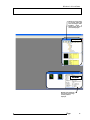
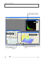
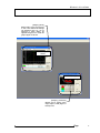
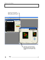
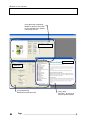
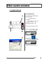
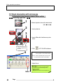
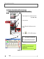
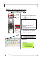
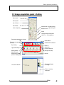
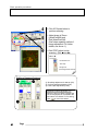
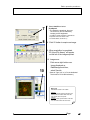
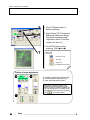
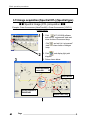
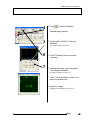
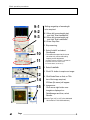
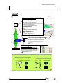
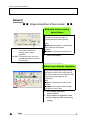
Quick Start
FLUOVIEW
FV1000
CONFOCAL LASER SCANNING
BIOLOGICAL MICROSCOPE
FV10-ASW 【Ver1.3】
Petition
Thank you for your purchase of Olympus microscope at this time.
Prior to using this microscope, read this instruction manual for sure to utilize full-fledged
performance of this microscope and ensure customer’s safety.
In addition, read section “Safety Guide” and “Hardwarel” of User’s Manual – FLUOVIEW FV1000
as well as instruction manual for microscope to understand how to use the equipment thoroughly.
To use laser system correctly, read instruction manuals that come with each laser equipment and
light power system.
Hold this manual by your side when using this microscope all the time and keep it with care after reading.
AX7284
Caution
1. Part or whole of this software as well as manual shall not be used or duplicated without consent.
2. Contents described in this manual are subject to change without notice in future.
Registered trademark
OLYMPUS, FLUOVIEW and LSM are of our registered trademark.
CONTENTS
1 About this manual㩷㩷㩷㩷㩷㩷㩷㩷㩷㩷㩷㩷㩷㩷㩷㩷㩷㩷㩷㩷㩷㩷㩷㩷㩷㩷㩷㩷㩷㩷㩷㩷㩷㩷㩷㩷㩷㩷㩷㩷㩷㩷㩷㩷㩷㩷㩷㩷㩷㩷㩷㩷㩷㩷㪈
2 Windows in this software㩷㩷㩷㩷㩷㩷㩷㩷㩷㩷㩷㩷㩷㩷㩷㩷㩷㩷㩷㩷㩷㩷㩷㩷㩷㩷㩷㩷㩷㩷㩷㩷㩷㩷㩷㩷㩷㩷㩷㩷㩷㩷㩷㪈
3 Basic operation procedures㩷㩷㩷㩷㩷㩷㩷㩷㩷㩷㩷㩷㩷㩷㩷㩷㩷㩷㩷㩷㩷㩷㩷㩷㩷㩷㩷㩷㩷㩷㩷㩷㩷㩷㩷㩷㩷㩷㪈㪊
13
3.1. System Start Up
3.2.Visual observation with microsocpe
(Differential Interference Image Observation ) - Erecting type BX -
14
3.3.Visual observation with microscope
(Differential Interference Image Observation ) - Erecting type BXWI -
15
3.4.Visual observation with microscope
(Differential Interference Image Observation ) - Inverted type IX -
16
3.5.Visual observation with microscope
(Fluorescent image observation) - Erecting type BX, BXWI -
17
3.6.Visual observation with microscope
(Fluorescent image observation) - Inverted type IX -
18
3.7.Image acquisition panel - Outline
19
3.8.Image acquisition (Single dyeing color XY)
20
3.9.Image acquisition (Double dyeing color XY) - Simultaneous scan version -
23
3.10.Image acquisition (Double dyeing color XY) - Sequential Scan Version -
26
3.11.Image acquisition (Single dyeing color + DIC‫ޓ‬XY)
29
3.12.Image acquisition (Double dyeing color XYZ)
32
3.13.Image acquisition (Spectral XYL) (Spectral type)
34
3.14. 2D Operation Panel Outline
37
3.15.File open
37
3.16. Display of XYZ Image (Cross-section image overlap)
38
3.17.Putting Scale bar
39
3.18. 3D Display
40
3.19.Rotation of cubic image
42
3.20.Fluorescence separation
unmixing (Spectral type)
- Part 1: In case that Dye place for each fluorescence is known -
44
CONTENTS
3.21.Fluorescence separation
unmixing (Spectral type)
- Part 2: In case that control sample is used 3.22.Fluorescence separation
45
unmixing (Spectral type)
- Part 3:In case that number of fluorescent dye kinds only is known (Blind Unmixing) - 47
3.23.Image save
48
3.24.Save to CD-R
49
3.25.System shut down
50
Annex 1 Relationship between confocal principle and tuning mechanism
51
Annex 2 Image acquisition of less noises
52
Annex 3 Method to change width or position of slit in manual mode
53
㪘㪹㫆㫌㫋㩷㫋㪿㫀㫊㩷㫄㪸㫅㫌㪸㫃
1 About this manual
This manual describes about windows that can be displayed (Section 2) and simple operation procedures
(Section 3).
For further details of each window, see Online Help that appears through [Help] – [Help].
2 Windows in this software
Window used on FV10-ASW (Application Software) is individually introduced.
Page
1
㪮㫀㫅㪻㫆㫎㫊㩷㫀㫅㩷㫋㪿㫀㫊㩷㫊㫆㪽㫋㫎㪸㫉㪼
Window to acquire image
Window to set image
acquisition
Acquisition
setting
Image
acquisition
Bleach setting
Spectrometer
setting
Window that opens when button
for “Image Acquisition” is
pressed and it is used for bleach
setting.
㪉
Page
Window that opens when button
for “Image Acquisition” is pressed and
it is used for spectrometer setting.
㪮㫀㫅㪻㫆㫎㫊㩷㫀㫅㩷㫋㪿㫀㫊㩷㫊㫆㪽㫋㫎㪸㫉㪼
Window that opens when button
for
“Image Acquisition” is pressed and it is
used for light path setting.
Window that opens when button
for
“Image Acquisition” is pressed and it is
used for Dye setting.
㪣㫀㪾㪿㫋㩷㪧㪸㫋㪿㩷㪪㪼㫋㫋㫀㫅㪾
㪛㫐㪼㩷㪪㪼㫋㫋㫀㫅㪾
Acquisition Program/Run
Microscope Control
[Device] – [Time Controller]
Window that the acquisition is
programmed and the process is
executed.
[Device] - [Microscope Controller]
Window to control microscope main
unit and motorized section attached to
the microscope main unit.
Page
3
㪮㫀㫅㪻㫆㫎㫊㩷㫀㫅㩷㫋㪿㫀㫊㩷㫊㫆㪽㫋㫎㪸㫉㪼
Window that opens
when button
for
“2D Setting” is
pressed and it is
used to display
intensity profile of 2D
image in vertical
direction.
Window that opens
Window to display 2D. When “Live View”
appears, the image being acquired will be
displayed.
when button
㩷for
“2D Display” is
pressed and it is used
for 2D display setting.
㪝㫆㫉㩷㪊㪛㩷㪭㫀㪼㫎
2D Setting
2D Display
LUT Setting
Window that opens when
button
for “2D
Setting” is pressed and it
is used to display
intensity profile of 2D
image in horizontal
direction.
㪋
Page
Window that opens
when button
for
“2D Setting” is
pressed and it is used
for LUT setting that
changes image display
color.
㪮㫀㫅㪻㫆㫎㫊㩷㫀㫅㩷㫋㪿㫀㫊㩷㫊㫆㪽㫋㫎㪸㫉㪼
Window to load an image
by selecting folder that
saves the images. When
thumbnail
image
is
double-clicked, the file is
called and displayed.
Explorer
㪛㪸㫋㪸㩷㪤㪸㫅㪸㪾㪼㫉
Window where thumbnail
and property of the image
currently loaded is
displayed.
Page
5
㪮㫀㫅㪻㫆㫎㫊㩷㫀㫅㩷㫋㪿㫀㫊㩷㫊㫆㪽㫋㫎㪸㫉㪼
[Analysis] – [Single] 䋭 [Histogram]
Window that Histogram is displayed.
Histogram
ROI Measurement
Intensity Profile Display
[Analysis] – [Single] – [Intensity Profile]
[Analysis] - [Single]䋭[Measurement]
Window that ROI (Region of Interest)
is measured.
㪍
Page
Window that intensity profile inside ROI selected is
displayed.
㪮㫀㫅㪻㫆㫎㫊㩷㫀㫅㩷㫋㪿㫀㫊㩷㫊㫆㪽㫋㫎㪸㫉㪼
[Analysis] - [Series]
Window where series image analysis
is done. Time transition for Average
and Integration value, etc., can be
displayed in graph. Setting the
applicable image to “Live” causes the
graph to appear in real-time.
Series Analysis
LivePlot
Line Series Analysis
[Analysis] – [Line Series]
Window used to perform series
image analysis on ROI (Region of
Interest) of line.
Page
7
㪮㫀㫅㪻㫆㫎㫊㩷㫀㫅㩷㫋㪿㫀㫊㩷㫊㫆㪽㫋㫎㪸㫉㪼
[Processing] – [Image Calculation]
Window used to perform operations
between images. Logic and
arithmetic operation for image
intensity can be done.
[Processing] - [Filter setting]
Window to enhance the image.
Operation
between
images
Filter process
Ratio/Concentration
Operation
Binary process
[Processing] – [Threshold]
Window to turn the image to
binary data.
[Processing] - [Ratio/Concentration]
1.Image of intensity ratio between channels converted to
intensity value is created.
2.Image of ion concentration of specimen converted to
intensity value is created.
㪏
Page
㪮㫀㫅㪻㫆㫎㫊㩷㫀㫅㩷㫋㪿㫀㫊㩷㫊㫆㪽㫋㫎㪸㫉㪼
[Processing] – [Spectral Deconvolution]
Window for spectral deconvolution (the
process to separate fluorescent from image
of multi-dyeing specimen).
Spectral Deconvolution (Fluorescent separation)
Channels Edition
Image Connection
Image Extraction
䌛Processing䌝 - 䌛Edit Experiment䌝
㪚㫆㫃㫆㪺㪸㫃㫀㫑㪸㫋㫀㫆㫅
[Processing] - [Colocalization]
1.Channel composition/extraction can
be done.
It is the window to see how the
intensity is overlapping.
2.Image can be connected each other.
For example, it is possible to see
what extent the bright area of Ch1 is
overlapping with the bright area of
Ch2 quantitatively.
3.Image can be extracted.
Page
9
㪮㫀㫅㪻㫆㫎㫊㩷㫀㫅㩷㫋㪿㫀㫊㩷㫊㫆㪽㫋㫎㪸㫉㪼
[Processing] – [Correcting Z Gaps]
Window where Z position shift
between image channels is corrected.
Z Shift Correction
Pixel Shift Correction
䌛Processing䌝 - 䌛Correcting Pixel Gaps䌝
Window where pixel position is corrected in
XY direction, if it is shifted, between light
receiving channels while image is being
acquired.
㪈㪇
Page
㪮㫀㫅㪻㫆㫎㫊㩷㫀㫅㩷㫋㪿㫀㫊㩷㫊㫆㪽㫋㫎㪸㫉㪼
Window for 3D display that opens
when 2D Display
button is pressed.
3D Display
Page
11
㪮㫀㫅㪻㫆㫎㫊㩷㫀㫅㩷㫋㪿㫀㫊㩷㫊㫆㪽㫋㫎㪸㫉㪼
[Tool] - [Microscope Configuration]
Window for setting microscope main
unit and motorized section attached
to microscope main unit.
Microscope Setting
Online Help
Maintenance
[Tool] – [Maintenance]
Maintenance of system can be done.
㪈㪉
Page
[Help] – [Help]
Online Help. See here for the
details of operation methods.
㪙㪸㫊㫀㪺㩷㫆㫇㪼㫉㪸㫋㫀㫆㫅㩷㫇㫉㫆㪺㪼㪻㫌㫉㪼㫊㩷
㪊 㪙㪸㫊㫀㪺㩷㫆㫇㪼㫉㪸㫋㫀㫆㫅㩷㫇㫉㫆㪺㪼㪻㫌㫉㪼㫊㩷
㩷
3.1.System Start Up
1
䋱. Turn computer to ON.
2. Turn FV10-PSU to ON.
3. Turn BX-UCB or IX2-UCB to ON.
4. Turn laser to ON.
(Turn key switch.)
4-1. Multi Ar
䋨458nm䊶488nm䊶514nm䋩 ON
4-2. HeNe䋨G䋩䋨543nm䋩 ON
4-3. HeNe䋨R䋩䋨633nm䋩 ON
5. Turn mercury lamp power to ON.
5
4
7
6. Enter user name/password and
logon to WindowsXP.
User name: Administrator
Password: fluoview
7. Double-click
and
FV10-ASW software starts up.
User name: Administrator
Password: Administrator
It takes a certain period of time for start up.
1
㩷
Page
㪈㪊
㪙㪸㫊㫀㪺㩷㫆㫇㪼㫉㪸㫋㫀㫆㫅㩷㫇㫉㫆㪺㪼㪻㫌㫉㪼㫊㩷
㩷
㩷
3.2.Visual observation with microsocpe
(Differential Interference Image Observation )
䂓 䂓 Erecting type BX 䂓 䂓
1
Hand switch
2
1. Select objective lens with hand switch.
(Ref: 䂓Memo䂓䋩
2. Insert polarizer.
DIC element
3
3. Insert differential interference prism
slider.
Differential interference
contrast is adjusted with
this knob.
4
4. Click
of FV10-ASW software.
Note 1: Light of halogen lamp is adjusted, using
TD Lamp slider on FV10-ASW software.
Note 2: Check if the filter turret is set to 6. DIC.
If not, press DICT button of hand switch.
5. Adjust focus.
Note 1
2
㪈㪋㩷
䂓 Memo 䂓
When magnification change is required hereafter,
do procedure 1 only and the followings will be
changed accordingly:;
䃂 Objective lens
䃂 Optimum DIC element to each objective lens
㩷
Page
㪙㪸㫊㫀㪺㩷㫆㫇㪼㫉㪸㫋㫀㫆㫅㩷㫇㫉㫆㪺㪼㪻㫌㫉㪼㫊㩷
㩷
㩷
3.3.Visual observation with microscope
(Differential Interference Image Observation )
䂓 䂓 Erecting type BXWI 䂓 䂓
1
1. Select objective lens.
DIC element
3
2
2. Insert polarizer and select DIC
element.
3. Insert differential interference prism
slider and select differential
interference analyzer (DICT).
Photo shows BX61.
Differential interference
contrast is adjusted with
this knob.
4. Click
4
of FV10-ASW software.
Note 1: Light of halogen lamp is adjusted, using
TD Lamp slider on FV10-ASW software.
Note 2: Check if the filter turret is set to 6. DICT.
If not, press DICT button of hand switch.
5. Adjust focus.
3
Note 1
㩷
Page
㪈㪌
㪙㪸㫊㫀㪺㩷㫆㫇㪼㫉㪸㫋㫀㫆㫅㩷㫇㫉㫆㪺㪼㪻㫌㫉㪼㫊㩷
㩷
㩷
3.4.Visual observation with microscope
(Differential Interference Image Observation )
䂓 䂓 Inverted type IX 䂓 䂓
1
Hand switch
DIC element
2
1. Select objective lens with hand switch.
(Ref: 䂓Memo䂓)
2. Insert polarizer.
3
3. Insert differential interference prism
slider.
Differential interference
contrast is adjusted with
this knob.
4
4. Click
of FV10-ASW software.
Note 1: Light of halogen lamp is adjusted, using
TD Lamp slider on FV10-ASW software.
Note 2: Check if the filter turret is set to 6. DIC.
If not, press DICT button of hand switch.
5. Adjust focus.
䂓 Memo 䂓
When magnification change is required hereafter,
do procedure 1 only and the followings will be
changed accordingly;
䃂 Objective lens
䃂 Optimum DIC element for each objective lens
Note 1
4
㪈㪍㩷
㩷
Page
㪙㪸㫊㫀㪺㩷㫆㫇㪼㫉㪸㫋㫀㫆㫅㩷㫇㫉㫆㪺㪼㪻㫌㫉㪼㫊㩷
㩷
㩷
3.5.Visual observation with microscope
(Fluorescent image observation)
䂓 䂓 Erecting type BX, BXWI 䂓 䂓
3
Hand switch
1
1. Select objective lens with hand switch.
2䋮Click
of FV10-ASW software.
Note 1
Note 2
Note 1: Operation in procedure 2 turns the
mode to fluorescent visual mode.
At this moment, mechanical shutter of
mercury lamp will open. Be careful.
(Mercury lamp shutter – Close is done
from hand switch.)
Note 2: Verify that the differential interference
slider is pulled out.
3.
2
Select fluorescent filter with hand
switch. (Ref: 䂓Memo䂓䋩
䂓 Memo 䂓
About fluorescent filter
NIBA: Blue excitation/Green fluorescent
(Example: FITC, EGFP etc.)
WIG: Green excitation/Red fluorescent
(Example: Rhodamine, DsRed. etc.)
4. Adjust focus.
5
㩷
Page
㪈㪎
㪙㪸㫊㫀㪺㩷㫆㫇㪼㫉㪸㫋㫀㫆㫅㩷㫇㫉㫆㪺㪼㪻㫌㫉㪼㫊㩷
㩷
㩷
3.6.Visual observation with microscope
(Fluorescent image observation)
䂓 䂓 Inverted type IX 䂓 䂓
3
Hand switch
1
1. Select objective lens with hand switch.
䋲䋮Click
of FV10-ASW software.
Note 1: Operation in procedure 3 turns the
mode to fluorescent visual mode.
At this moment, mercury lamp mechanical
shutter will open. Be careful.
(It is recommended that the mercury lamp
manual shutter is set to Close 䃂
beforehand.)
Note 2: Verify that the differential interference
slider is pulled out.
Note 2
Note 1 & 3
2
3.
Select fluorescent filter with hand
switch. (Ref: 䂓Memo䂓䋩
Note 3: When viewing through microscope,
verify whether or not the mercury lamp
mechanical shutter is set to Open 䂾.
4. Adjust focus.
䂓 Memo 䂓
About fluorescent filter
NIBA: Blue excitation/Green fluorescent
(Example: FITC, EGFP, etc.)
WIG : Green excitation/Red fluorescent
(Example: Rhodamine, DsRed, etc.)
6
㪈㪏㩷
㩷
Page
㪙㪸㫊㫀㪺㩷㫆㫇㪼㫉㪸㫋㫀㫆㫅㩷㫇㫉㫆㪺㪼㪻㫌㫉㪼㫊㩷
㩷
㩷
3.7.Image acquisition panel - Outline
Scan mode
Scan speed
No. of Pixels
Zoom䋧Pan
Laser output adj.
Lambda scan condition setting
(Spectral type)
Objective lens
Focus
TimeInterval䋧TimeNumber
䋨at XYT or XT acquisition)
Transmitted observation (Visual)
Scan buttons
Fluorescent observation
(Visual)
Dye setting
Light path setting
Slit adjustment
(Spectral type)
SIM Scanner setting
(Case of adding ASU)
Live View Window
XYZ/XYT/XYL selection
Each Ch
device adj.
Confocal aperture
Halogen lamp adj
Kalman
Thumbnail display
Of Image
Files on memory
displayed
7
㩷
Page
㪈㪐
㪙㪸㫊㫀㪺㩷㫆㫇㪼㫉㪸㫋㫀㫆㫅㩷㫇㫉㫆㪺㪼㪻㫌㫉㪼㫊㩷
㩷
㩷
3.8.Image acquisition (Single dyeing color XY)
䂓䂓 1 slice of image acquisition (XY plane) (Fluorescent image only)䂓䂓
Example: Single dyeing with green fluorescence (FITC)
1
1. Click
of FV10-ASW software
and set it to “not pressed” state
and close shutter of fluorescent
lamp.
Click
and set it to “not pressed”
state and close shutter of halogen
lamp.
2
2. Click DyeList button and doubleclick fluorescent reagent (FITC)
that should be observed from
DyeList panel.
When reselecting, double-click the
fluorescent dye in AssignDyes one
time to clear it, and then, perform
operation in procedure 2.
3
3. Click Apply button.
(DyeList panel can be closed with䇮
Close button.)
- In case of Spectral type When this operation is done, the
fluorescent wavelength suit to
Fluorescent Dye selected is defined.
Window after DyeApply is clicked
8
㪉㪇㩷
Moreover, the fluorescent wavelength
is manually changeable.
For further details, see Annex 3.
㩷
Page
㪙㪸㫊㫀㪺㩷㫆㫇㪼㫉㪸㫋㫀㫆㫅㩷㫇㫉㫆㪺㪼㪻㫌㫉㪼㫊㩷
㩷
㩷
4
4. Click XY Repeat button to
perform scanning.
5
5. Adjust green (FITC) image.
(See below for outline of image
adjustment. For further details,
see Annex 1.)
6
6. Click STOP button to stop
scanning. (Ref: 䂓Memo䂓)
䂓 Memo䂓
About scan button
: Consecutive scan
: Scan stop
: Rough scan
(Lines skipped and scanned)
Outline of image adjustment
཰
ཱ
཰ Sensitivity of detector adjustment (HV)
ཱ Confocal aperture adjustment (CA)
ི Laser output adjustment (Laser)
Adjustment method (Example: HV)
When any place on slider is clicked, the
HV can be jumped UP or DOWN to the
point where it is clicked. For fine tuning,
click
or use mouse wheel.
ི
9
㩷
Page
㪉㪈
㪙㪸㫊㫀㪺㩷㫆㫇㪼㫉㪸㫋㫀㫆㫅㩷㫇㫉㫆㪺㪼㪻㫌㫉㪼㫊㩷
㩷
㩷
7. Select AutoHV and select
7
ScanSpeed.
The slower the speed set, the more
the noise only can be reduced by
keeping current brightness.
(In addition, Kalman integration is available as a
8
separate method to remove noise.
For further details, see Annex 2.)
8. Click XY button to acquire an image.
9. When acquisition is completed,
“2D View-(File Name)” will appear
on title bar of the image acquired.
10. Image save:
Click mouse right button over
Image displayed on
DataManager and then,
10
select SaveAs.
(Save as Type “oib” or “oif” is the dedicated
file format for FV10-ASW software.)
䂓Memo 䂓
Dedicated file format for FV10-ASW
OIF type:
Folder that contains images (16bit TIFF) and
attached file are created. Unless these two
exist, the file cannot be opened.
OIB type:
File that contains a plural number of OIF files.
It is convenience when files are moved.
10
㪉㪉㩷
㩷
Page
㪙㪸㫊㫀㪺㩷㫆㫇㪼㫉㪸㫋㫀㫆㫅㩷㫇㫉㫆㪺㪼㪻㫌㫉㪼㫊㩷
㩷
㩷
3.9.Image acquisition (Double dyeing color XY)
䂓䂓 1 slice of image acquisition (XY plane) (Fluorescent image only) 䂓䂓
Example: Green fluorescence (Alexa488) + Red fluorescence (Alexa546)
Double dyeing simultaneous scan version
1
2
1. Click
of FV10-ASW software
and set it to “not pressed” state
and close shutter of fluorescent
lamp.
Click
and set it to “not
pressed” state and close shutter
of halogen lamp.
2. Click DyeList button and select
fluorescent reagent (Alexa488,
Alexa546) from DyeList
panel and double-click it.
When reselecting, double-click the
fluorescent reagent in AssignDyes
one time to delete it and then, do
procedure 2.
3. Click Apply button.
3
( DyeList panel can be closed
with Close button.)
- In case of Spectral type When this operation is done, the
fluorescent wavelength suit to
Fluorescent Dye selected is defined.
11
Window after DyeApply clicked
Moreover, the fluorescent wavelength
is manually changeable.
For further details, see Annex 3.
㩷
Page
㪉㪊
㪙㪸㫊㫀㪺㩷㫆㫇㪼㫉㪸㫋㫀㫆㫅㩷㫇㫉㫆㪺㪼㪻㫌㫉㪼㫊㩷
㩷
㩷
4
5
6
4. Click XY Repeat button to
perform scanning.
5. Adjust image of Green
(AlexaFluor488) and
Red (AlexaFluor546).
(See below regarding outline of
image adjustment. For further
details, see Annex 1.)
6. Click STOP button to stop
scanning. (Ref: 䂓Memo䂓)
䂓 Memo 䂓
Scan buttons
: Consecutive scan
: Scan stop
: Rough scan
(Lines skipped and scanned)
Outline of image adjustment
཰
ཱ
཰ Sensitivity adjustment of detector (HV)
ཱ Confocal aperture adjustment (CA)
ི Laser output adjustment (Laser)
Adjustment method (Example: HV)
When any place on slider is clicked, the
HV can be jumped UP or DOWN to the
point where it is clicked. For fine tuning,
click
or use mouse wheel.
ི
12
㪉㪋㩷
㩷
Page
㪙㪸㫊㫀㪺㩷㫆㫇㪼㫉㪸㫋㫀㫆㫅㩷㫇㫉㫆㪺㪼㪻㫌㫉㪼㫊㩷
㩷
㩷
7
7. Select AutoHV and select
ScanSpeed.
The slower the speed set, the more
the noise only can be reduced by
keeping current brightness.
(In addition, Kalman integration is available as
a separate method to remove noise.
For further details, see Annex 2.)
8
8. Click XY button to acquire an image.
9. When acquisition is completed,
“2D View-(File Name)” will appear
on title bar of the image acquired.
10. Image save:
Click mouse right button over
Image displayed on
DataManager and then,
10
select SaveAs.
(Save as Type “oib” or “oif” is the dedicated
file format for FV10-ASW software.)
䂓Memo 䂓
Dedicated file format for FV10-ASW
OIF type:
Folder that contains images (16bit TIFF) and
attached file are created. Unless these two
exist, the file cannot be opened.
OIB type:
File that contains a plural number of OIF files.
It is convenience when files are moved.
13
㩷
Page
㪉㪌
㪙㪸㫊㫀㪺㩷㫆㫇㪼㫉㪸㫋㫀㫆㫅㩷㫇㫉㫆㪺㪼㪻㫌㫉㪼㫊㩷
㩷
㩷
3.10.Image acquisition (Double dyeing color XY)
䂓䂓 1 slice of image acquisition (XY plane) (Fluorescent image only) 䂓䂓
Example: Green fluorescence (Alexa488) + Red fluorescence (Alexa546)
Double Dyeing Sequential Scan Version (Line Sequential introduced)
1
1. Click
of FV10-ASW software
and set it to “not pressed” state and
close shutter of fluorescent lamp.
Click
and set it to “not pressed”
state and close shutter of halogen
lamp.
2
2. Click DyeList button and select
fluorescent reagent (Alexa488,
Alexa546) from DyeList
panel and double-click it.
When reselecting, double-click the
fluorescent reagent in AssignDyes
one time to delete it and then, do
procedure 2.
3. Click Apply button.
3
( DyeList panel can be closed
with Close button.)
- In case of Spectral type When this operation is done, the
fluorescent wavelength suit to
Fluorescent Dye selected is defined.
14
㪉㪍㩷
Window after DyeApply clicked
Moreover, the fluorescent wavelength
is manually changeable.
For further details, see Annex 3.
㩷
Page
㪙㪸㫊㫀㪺㩷㫆㫇㪼㫉㪸㫋㫀㫆㫅㩷㫇㫉㫆㪺㪼㪻㫌㫉㪼㫊㩷
㩷
㩷
4
5
6
7
4. Check Sequential and select Line.
5 Click XY Repeat button to perform
scanning.
6. Adjust image of Green
(AlexaFluor488䋩 and
Red (AlexaFluor546).
(See below regarding image
adjustment outline. For further
details, see Annex 1.)
7. Click STOP button to stop
scanning
Outline of image adjustment
཰
ཱ
཰ Sensitivity adjustment of detector (HV)
ཱ Confocal aperture adjustment (CA)
ི Laser output adjustment (Laser)
Adjustment method (Example: HV)
When any place on slider is clicked, the
HV can be jumped UP or DOWN to the
point where it is clicked. For fine tuning,
click
or use mouse wheel.
ི
15
㩷
Page
㪉㪎
㪙㪸㫊㫀㪺㩷㫆㫇㪼㫉㪸㫋㫀㫆㫅㩷㫇㫉㫆㪺㪼㪻㫌㫉㪼㫊㩷
㩷
㩷
8. Select AutoHV and select
8
ScanSpeed.
The slower the speed set, the more
the noise only can be reduced by
keeping current brightness.
(In addition, Kalman integration is available
as a separate method to remove noise.
For further details, see Annex 2.)
9
9. Click XY button to acquire an image.
10. When acquisition is completed,
“2D View-(File Name)” will appear
on title bar of the image acquired.
11
11. Image save:
Click mouse right button over
Image displayed on
DataManager and then,
select SaveAs.
(Save as Type “oib” or “oif” is the dedicated
file format for FV10-ASW software.)
䂓Memo 䂓
Dedicated file format for FV10-ASW
OIF type:
Folder that contains images (16bit TIFF) and
attached file are created. Unless these two
exist, the file cannot be opened.
OIB type:
File that contains a plural number of OIF files.
It is convenience when files are moved.
16
㪉㪏㩷
㩷
Page
㪙㪸㫊㫀㪺㩷㫆㫇㪼㫉㪸㫋㫀㫆㫅㩷㫇㫉㫆㪺㪼㪻㫌㫉㪼㫊㩷
㩷
㩷
3.11.Image acquisition (Single dyeing color + DIC XY)
䂓䂓 1-slice Image (XY plane) acquisition
(Fluorescent Image + Differential Interference)䂓䂓
Example: Green fluorescence (FITC) + Differential Interference
1
1. Click
of FV10-ASW software
and set it to “not pressed” state and
close shutter of fluorescent lamp.
Click
and set it to “not pressed”
state and close shutter of halogen
lamp.
2
3
2. Click DyeList button and select
fluorescent reagent (FITC)
to be observed
from DyeList panel and double-click it.
When reselecting, double-click the
fluorescent dye in AssignDyes one
time to clear it and then, perform
procedure 2.
3. Click Apply button.
( DyeList panel can be closed
with Close button.)
4
4. Check TD1.
- In case of Spectral type When this operation is done, the
fluorescent wavelength suit to
Fluorescent Dye selected is defined.
Window after DyeApply clicked
17
Moreover, the fluorescent wavelength
is manually changeable.
For further details, see Annex 3.
㩷
Page
㪉㪐
㪙㪸㫊㫀㪺㩷㫆㫇㪼㫉㪸㫋㫀㫆㫅㩷㫇㫉㫆㪺㪼㪻㫌㫉㪼㫊㩷
㩷
㩷
5
5. Click XY Repeat button to
perform scanning.
6
6. Adjust Green (FITC) image and
differential interference image.
(See below regarding image
adjustment outline. For further
details, see Annex 1.)
7. Click STOP button to stop
scanning. (Ref: 䂓Memo䂓)
7
䂓 Memo 䂓
Scan buttons
: Consecutive scan
: Scan stop
: Rough scan
(Line skipped and scanned)
Outline of image adjustment
཰
ཱ
཰ Sensitivity adjustment of detector (HV)
ཱ Confocal aperture adjustment (CA)
ི Laser output adjustment (Laser)
Adjustment method (Example: HV)
When any place on slider is clicked, the
HV can be jumped UP or DOWN to the
point where it is clicked. For fine tuning,
click
or use mouse wheel.
ི
18
㪊㪇㩷
㩷
Page
㪙㪸㫊㫀㪺㩷㫆㫇㪼㫉㪸㫋㫀㫆㫅㩷㫇㫉㫆㪺㪼㪻㫌㫉㪼㫊㩷
㩷
㩷
8. Select AutoHV and select
8
ScanSpeed.
The slower the speed set, the more
the noise only can be reduced by
keeping current brightness.
(In addition, Kalman integration is available as
a separate method to remove noise.
For further details, see Annex 2.)
9
9. Click XY button to acquire an image.
10. When acquisition is completed,
“2D View-)File Name)” will appear
on title bar of the image acquired.
11
11. Image save:
Click mouse right button over
Image displayed on
DataManager and then,
select SaveAs.
(Save as Type “oib” or “oif” is the dedicated
file format for FV10-ASW software.)
䂓Memo 䂓
Dedicated file format for FV10-ASW
OIF type:
Folder that contains images (16bit TIFF) and
attached file are created. Unless these two
exist, the file cannot be opened.
OIB type:
File that contains a plural number of OIF files.
It is convenience when files are moved.
19
㩷
Page
㪊㪈
㪙㪸㫊㫀㪺㩷㫆㫇㪼㫉㪸㫋㫀㫆㫅㩷㫇㫉㫆㪺㪼㪻㫌㫉㪼㫊㩷
㩷
㩷
3.12.Image acquisition (Double dyeing color XYZ)
䂓䂓 Consecutive Cross-section Image (XYZ) Acquisition (Fluorescent Image only)䂓䂓
Example:Green fluorescence (Alexa488)+Red fluorescence (Alexa546) Double Dyeing
Cross-section image acquired with Line Sequential scanning
3
4
1. Perform procedures 1 through 7
described in page 26 and 27.
Upper and lower limit of consecutive
cross-section image is determined here.
5
2. Enter StepSize and tick the box.
6
7
3. Click XY Repeat button to perform
scanning.
4. Click
or
to bring the object
in out of focus.
5. When sample upper limit is displayed
on the sample, click Set button.
6. Click
or
to bring the object
in out of focus.
2
7. When sampler lower limit is displayed
on the sample, click Set button.
8. Click Stop button and stop scanning.
8
20
㪊㪉㩷
㩷
Page
㪙㪸㫊㫀㪺㩷㫆㫇㪼㫉㪸㫋㫀㫆㫅㩷㫇㫉㫆㪺㪼㪻㫌㫉㪼㫊㩷
㩷
㩷
9. Select AutoHV and select
9
11
ScanSpeed.
The slower the speed set, the more
the noise only can be reduced by
keeping current brightness.
(In addition, Kalman integration is available as
a separate method to remove noise.
For further details, see Annex 2.)
10. Select Depth.
11. Click XYZ button to acquire an image
10
12. Click SeriesDone so that, on Title
bar of the image acquired,
2D View-(file name) will appear.
13. Image save:
12
Click mouse right button over
ImageIcon displayed on
DataManager and then, select
13
SaveAs.
(Save as Type “oib” or “oif” is the dedicated
file format for FV10-ASW software.)
䂓Memo 䂓
Dedicated file format for FV10-ASW
OIF type:
Folder that contains images (16bit TIFF) and
attached file are created. Unless these two
exist, the file cannot be opened.
OIB type:
File that contains a plural number of OIF files.
It is convenience when files are moved.
21
㩷
Page
㪊㪊
㪙㪸㫊㫀㪺㩷㫆㫇㪼㫉㪸㫋㫀㫆㫅㩷㫇㫉㫆㪺㪼㪻㫌㫉㪼㫊㩷
㩷
㩷
3.13.Image acquisition (Spectral XYL) (Spectral type)
䂓䂓 Spectral Image (XYL) Acquisition 䂓䂓
Example: Green fluorescence (AlexaFluor488) + Green fluorescence (YOYO-1)
Double dyeing
1
1. Click
of FV10-ASW software
and set it to “not pressed” state and
close shutter of fluorescent lamp.
Click
and set it to “not pressed”
state and close shutter of halogen
lamp.
2
3
2. Click
diagram.
and display light path
3. Set as shown below.
Select Excitation
Laser 488
Select Mirror
Select BS20/80 or
DM405/488
22
㪊㪋㩷
Select CHS1 only
㩷
Page
㪙㪸㫊㫀㪺㩷㫆㫇㪼㫉㪸㫋㫀㫆㫅㩷㫇㫉㫆㪺㪼㪻㫌㫉㪼㫊㩷
㩷
㩷
4
4. Click
button and display
SpectralSetting window.
5
5. Set slit width of CHS1 to 10nm (as
example).
(To change slit width, see Annex 3.)
6
7
6. Click XY Repeat button to perform
scanning.
7. Viewing the image, move slit position
to the brightest position.
(To change slit position, see Annex 3.)
Note: Leave slit width to 10nm “as is”
and move position only.
8. Adjust the image.
(Regarding image adjustment, see Annex 1.)
23
㩷
Page
㪊㪌
㪙㪸㫊㫀㪺㩷㫆㫇㪼㫉㪸㫋㫀㫆㫅㩷㫇㫉㫆㪺㪼㪻㫌㫉㪼㫊㩷
㩷
㩷
9-1
9-2
9-3
9. Setting range/step of wavelength
to be acquired.
9-1䋺Move slit to wavelength start
and click “Start LambdaSet”.
9-2䋺Move slit to wavelength end
and click “End LambdaSet”.
9-3䋺Enter Step Size.
10. Stop scanning.
10
11
13
11. Select AutoHV and select
ScanSpeed.
The slower the speed set, the more
the noise only can be reduced by
keeping current brightness.
(In addition, Kalman integration is available as
a separate method to remove noise.
For further details, see Annex 2.)
12. Select Lambda.
13. Click XYL button to acquire an image.
12
14
15
14. Click SeriesDone so that, on Title
bar of the image acquired,
2DView-(file name) will appear.
15. Image save:
Click mouse right button over
ImageIcon displayed on
DataManager and then, select
SaveAs.
(Save as Type “oib” or “oif” is the dedicated
file format for FV10-ASW software.)
24
㪊㪍㩷
㩷
Page
㪙㪸㫊㫀㪺㩷㫆㫇㪼㫉㪸㫋㫀㫆㫅㩷㫇㫉㫆㪺㪼㪻㫌㫉㪼㫊㩷
㩷
㩷
3.14. 2D Operation Panel Outline
TEXT
Grid
Arrow
Scale
Bar
Point
When clicked, it changes alternately
ROI type
Ch1
Ch䋲
Display change
Zoom
1:1 Display
to match with
Window size
Frame feed
Animation
Fast feed
3D
Formation
Projection
change
End Section
Fix
Start Section
Fix
Color bar
3.15.File open
1
1. Double-click a file that should be
opened from Explorer.
25
㩷
Page
㪊㪎
㪙㪸㫊㫀㪺㩷㫆㫇㪼㫉㪸㫋㫀㫆㫅㩷㫇㫉㫆㪺㪼㪻㫌㫉㪼㫊㩷
㩷
㩷
3.16. Display of XYZ Image (Cross-section image overlap)
1
1. Click
and select
.
2
26
㪊㪏㩷
2. In case that this image is saved,
click mouse right button over the
image and select Save Display and
save it with a name assigned.
㩷
Page
㪙㪸㫊㫀㪺㩷㫆㫇㪼㫉㪸㫋㫀㫆㫅㩷㫇㫉㫆㪺㪼㪻㫌㫉㪼㫊㩷
㩷
㩷
3.17.Putting Scale bar
1
1. Click
2
2. While left mouse button is clicked
over the image, drag the mouse and
release the button at proper point.
button.
Size change
3. While right or left handle is clicked,
move the mouse, left or right.
3
Change of character size,
color and style, etc.
4
4. After selecting ScaleBar, click
mouse right button over ScaleBar
and select “FormatSetting”.
5
5. In this Window, change portions
that must be changed.
27
㩷
Page
㪊㪐
㪙㪸㫊㫀㪺㩷㫆㫇㪼㫉㪸㫋㫀㫆㫅㩷㫇㫉㫆㪺㪼㪻㫌㫉㪼㫊㩷
㩷
㩷
3.18. 3D Display
1
Image is observed from
arbitrarily selected angle.
1. Click
button on 2D View(file name) image.
2. [3D-OLYMPUS FLUOVIEW]
window starts up and 3D View
will be built up.
3
3. Dragging mouse over the image,
observe the image from arbitrarily
selected angle.
o To save this image, see procedure
6 in next page.
4
Cross-section image at optional
angle is observed.
4. Click
5
and select
.
5. Dragging mouse over the image,
move, left or right, to see crosssection at optional angle.
o To save this image, see procedure
6 in next page.
28
㪋㪇㩷
㩷
Page
㪙㪸㫊㫀㪺㩷㫆㫇㪼㫉㪸㫋㫀㫆㫅㩷㫇㫉㫆㪺㪼㪻㫌㫉㪼㫊㩷
㩷
㩷
6
Image in procedure 3 or 5 is
saved.
6. Click
button.
7. 2D View-(file name) image appears.
8
8. Image save:
Click mouse right button over
Image displayed on
DataManager and then, select
SaveAs.
(Save as Type “oib” or “oif” is the dedicated
file format for FV10-ASW software.)
䂓Memo 䂓
Dedicated file format for FV10-ASW
OIF type:
Folder that contains images (16bit TIFF) and
attached file are created. Unless these two
exist, the file cannot be opened.
OIB type:
File that contains a plural number of OIF files.
It is convenience when files are moved.
29
㩷
Page
㪋㪈
㪙㪸㫊㫀㪺㩷㫆㫇㪼㫉㪸㫋㫀㫆㫅㩷㫇㫉㫆㪺㪼㪻㫌㫉㪼㫊㩷
㩷
㩷
3.19.Rotation of cubic image
1
1. Click
button on
2D View-(file name) image.
2. [3D-OLYMPUS FLUOVIEW]
window starts up and 3D View
will be built up.
3
3. Dragging mouse over the image,
observe the image from arbitrarily
selected angle.
Simplified animation
4
4. When
button is clicked
with long press mode, the image
turns with X-axis as rotation center.
When clicked again, the turn would
stop.
When
button is clicked
with long press mode, the image
turns with Y-axis as rotation center.
When clicked again, the turn would
stop.
When
button is clicked
with long press mode, the image
turns with Z-axis as rotation center.
When clicked again, the turn would
stop.
30
㪋㪉㩷
㩷
Page
㪙㪸㫊㫀㪺㩷㫆㫇㪼㫉㪸㫋㫀㫆㫅㩷㫇㫉㫆㪺㪼㪻㫌㫉㪼㫊㩷
㩷
㩷
5
6
When a rotation file is saved
as movie, 3D formation must
be executed as follows.
Let’s turn an image 180q as example.
5. Click
button.
6. Double-click Angle Rotation tab.
7
8
9
7. Select rotation angle axis.
8. Enter rotation angle.
Start䋽From what degree / End䋽
To what degree
Frame/s䋽Rotation speed /
Interval䋽per what degree
9. Select AVI File and click
Create.
10
10. Enter file name and click
Save.
31
㩷
Page
㪋㪊
㪙㪸㫊㫀㪺㩷㫆㫇㪼㫉㪸㫋㫀㫆㫅㩷㫇㫉㫆㪺㪼㪻㫌㫉㪼㫊㩷
㩷
㩷
3.20.Fluorescence separation - unmixing (Spectral type)
Part 1: In case that Dye place for each fluorescence is known
Fluorescent spectrum of each fluorescent dye are extracted from
XYL image where a plural number of fluorescent dyes having
fluorescent spectrum similar to each other exist and; with the said
fluorescent spectrum as reference, a method is presented here to
acquire a fluorescence separated image.
Example: Green fluorescence (AlexaFluor488) + Green fluorescence (YOYO-1)
2
3
4
5
1. Open XYL image file of
AlexaFluor488 + YOYO1 of
double dyeing.
2. Surround AlexaFluor488 and
YOYO1 region only with ROI.
3. Select SpectralDeconvolution
from Processing on menu bar.
4. Double-click ROI1 and ROI2
respectively.
5. Verify that Processing type is set
to “Normal” and BackGround
Correcting is turned “ON” and
then, click NewImage.
6. Image of fluorescent separation
can be acquired.
6
32
㪋㪋㩷
After fluorescence separation
(Unmixing), the assignment of
image to Ch is indicated.
Image after fluorescence separating (Unmixing)
㩷
Page
㪙㪸㫊㫀㪺㩷㫆㫇㪼㫉㪸㫋㫀㫆㫅㩷㫇㫉㫆㪺㪼㪻㫌㫉㪼㫊㩷
㩷
㩷
3.21.Fluorescence separation - unmixing (Spectral type)
Part 2: In case that control sample is used
Method to acquire a fluorescence separated image with
reference to fluorescent spectrum. The said spectrum are
extracted from one kind of fluorescent dye on XYL image.
Example: Green fluorescence (AlexaFluor488) + Green fluorescence (YOYO-1)
Double Dyeing
2
1. Open XYL image file of control
sample (the sample dyed with
AlexaFluor488 only).
3
2. Surround AlexaFluor488 region
with ROI.
4
3. Select SpectralDeconvolution
from Processing on menu bar.
4. Double-click ROI1.
5
Registered fluorescent spectral appears here.
33
6
5. Click SaveProfile.
6. Enter name to be saved and click
OK and the fluorescent spectral of
AlexaFluor488 is registered to
data base.
7. Perform the same operation, 1 to 6,
for YOYO1.
㩷
Page
㪋㪌
㪙㪸㫊㫀㪺㩷㫆㫇㪼㫉㪸㫋㫀㫆㫅㩷㫇㫉㫆㪺㪼㪻㫌㫉㪼㫊㩷
㩷
㩷
8
9
10
8. Open XYL image file of
AlexaFluor488 + YOYO1
of double dyeing.
9. Select SpectralDeconvolution
from Processing on menu bar.
10. Double-click AlexaFluor488 and
YOYO1 (previously registered)
from data base of fluorescent
spectrum.
11. Verify that Processing type is set
to “Normal” and BackGround
Correcting is turned “ON” and
then, click NewImage.
11
12. Image of fluorescence separated
can be acquired.
12
After fluorescence separation
(Unmixing), the assignment of
image to Ch is indicated.
Image after fluorescence separating (Unmixing)
34
㪋㪍㩷
㩷
Page
㪙㪸㫊㫀㪺㩷㫆㫇㪼㫉㪸㫋㫀㫆㫅㩷㫇㫉㫆㪺㪼㪻㫌㫉㪼㫊㩷
㩷
㩷
3.22.Fluorescence separation - unmixing (Spectral type)
Part 3: In case that number of fluorescent dye kinds only is known
known (Blind Unmixing)
Unmixing)
Method to acquire a fluorescence separated image with a little
information such as number of fluorescent dye kinds only known as a
hint from XYL image where a plural number of fluorescent dyes
having fluorescent spectrum similar to each other exist.
Example: Sample having 2 kinds of unknown fluorescent dyes
1. Open XYL image file of sample
that has 2 kinds of unknown
fluorescent dyes.
2
3
4
2. Select SpectralDeconvolution
from Processing on menu bar.
3. Put check marks at 2 places for
Calculate check box.
(When 3 kinds of fluorescent Dyes
exist, click 3 places to put check
marks.)
4. Verify that Processing type is set
to “Blind” BackGround Correcting
is turned “ON” and then, click
NewImage.
5. Image of fluorescence separated
can be acquired.
5
After fluorescence separation
(Unmixing), the assignment of
image to Ch is indicated.
Image after fluorescence separating (Unmixing)
35
㩷
Page
㪋㪎
㪙㪸㫊㫀㪺㩷㫆㫇㪼㫉㪸㫋㫀㫆㫅㩷㫇㫉㫆㪺㪼㪻㫌㫉㪼㫊㩷
㩷
㩷
3.23.Image save
Each channel for XY or XYZ
Image is converted to TIFF.
1
1. Click mouse right button over
ImageIcon displayed on
DataManager and select
Export.
2. Set Save as Type to TIFF and
save.
Other type, BMP/JPEG/PNG can be selected.
䋲
䋳
Merge image of XY or XYZ
Image is converted to TIFF.
1. Click mouse right button over
ImageIcon displayed on
DataManager and select
Export.
2. Set Save as Type to TIFF.
3. Check MergeChannel and
save.
Other type, BMP/JPEG/PNG can be selected.
**********************************************************************************
1
2
Image with Scale bar is
converted to BMP.
1. Click mouse right button over image.
2. Select Save Display and save
the image with a name assigned.
Movie is converted to AVI.
1. Click mouse right button over image.
2. Select Save as AVI and save
the image with a name assigned.
36
㪋㪏㩷
㩷
Page
㪙㪸㫊㫀㪺㩷㫆㫇㪼㫉㪸㫋㫀㫆㫅㩷㫇㫉㫆㪺㪼㪻㫌㫉㪼㫊㩷
㩷
㩷
3.24.Save to CD-R
1. Insert CD-R media.
2
2. Click OK.
3
4
5
3. Select a file and move it to Window
for CD-R with drag-and-drop
technique.
4. Click Write these files to CD.
5. Click Next.
6. Write will start.
6
7. Click Finish so that the save to CD-R
is completed.
7
37
㩷
Page
㪋㪐
㪙㪸㫊㫀㪺㩷㫆㫇㪼㫉㪸㫋㫀㫆㫅㩷㫇㫉㫆㪺㪼㪻㫌㫉㪼㫊㩷
㩷
㩷
3.25.System shut down
1
1. Shut donw FV10-ASW software with
File/Exit.
2. Shut down WindowsXP.
཰ Select Start - Shut Down.
2
ཱ Select “Shutdonwn” on
ShutDownWindow and
click OK.
3. Turn FV10-PSU to OFF.
4. Turn BX-UCB or IX2-UCB to
OFF.
5. Turn laser to OFF.
(Return key switch to OFF position)
5-1䋮Multi Ar
䋨458nm䊶488nm䊶514nm䋩 OFF
5-2䋮HeNe䋨G䋩䋨543nm䋩 OFF
5-3䋮HeNe䋨R䋩䋨633nm䋩 OFF
6
5
38
㪌㪇㩷
6. Turn mercury lamp power to OFF.
㩷
Page
㪙㪸㫊㫀㪺㩷㫆㫇㪼㫉㪸㫋㫀㫆㫅㩷㫇㫉㫆㪺㪼㪻㫌㫉㪼㫊㩷
㩷
㩷
Annex 1
䂓 䂓 Relationship between confocal principle and tuning mechanism 䂓 䂓
HV: Sensitivity adjustment
of detector (Voltage)
Setting value n ! Sensitivity n ! Image Brightness n
(But, noises are getting noticeable.)
It is recommended that the voltage is set at about 700V or less.
button: changes by 1V step.
(1V in case of transmitted image)
Gain adjustment (x)
Setting value n ! Image Brightness n
Image gets brighter with setting value.
button: changes by x0.001
OffSet adjustment (%)
Setting value n ! Image Brightness p
button: changes by 1%
C.A.: Confocal aperture adjustment (Pm)
Setting value n ! C.A. Size n ! Image Brightness n
(But, optical cross-section is getting thicker).
It is recommended that C.A. Is used with Auto.)
When C.A. should return to default setting after move,
press Auto again.
button: changes by 1Pm.
M_Ar or HeNeG䇮HeNeR:
Laser output adjustment (%)
Setting value n ! Output strength n ! Brightness n
(But, fluorescent discoloring is getting larger.)
Use with a value as small as possible recommended.
button; changes by 0.1%
䂓 Memo 䂓
Relationship between confocal aperture
and optical cross-section, image brightness
C.A.
Cross-section Image brightness
thickness
Relationship between laser output/
detector sensitivity and image brightness
M_Ar
PMT
Image brightness
39
㩷
Page
㪌㪈
㪙㪸㫊㫀㪺㩷㫆㫇㪼㫉㪸㫋㫀㫆㫅㩷㫇㫉㫆㪺㪼㪻㫌㫉㪼㫊㩷
㩷
㩷
Annex 2
䂓 䂓 Image acquisition of less noises 䂓 䂓
Method to make scanning
speed slower
Set scanning speed slower so that
an image can be acquired without
detecting noises from the beginning.
AutoON: The slower it is set, the more
noise can be removed by
keeping current image
brightness.
AutoOFF: The slower it is set, the more
it is getting brighter and noise is
also removed.
Merit:
䃂 With Kalman integration, comparatively
sharp image can be acquired.
Demerit:
䃂 Speed of scanning at one time is slow.
1. Select ScanSpeed.
**********************************************************************************
Method to use Kalman Integration
Images are averaged while image is being
acquired for number of times specified. As
the results, noises are also averaged so that
roughness of whole image can be
suppressed.
Merit:
䃂 Speed of scanning at one time is fast.
Demerit:
䃂 Images are averaged so that an image
may get dim, more or less.
1. Click Kalman and select
Line or Frame.
2. Enter number of integration times
for the image (number of scanning
cycles).
40
㪌㪉㩷
㩷
Page
㪙㪸㫊㫀㪺㩷㫆㫇㪼㫉㪸㫋㫀㫆㫅㩷㫇㫉㫆㪺㪼㪻㫌㫉㪼㫊㩷
㩷
㩷
Annex 3
䂓 䂓 Method to change width or position
of slit in manual mode 䂓 䂓
1
1. Click
button and display
SpectralSetting window.
2. Using
or
, move
left or right.
2
Spectral of fluorescent dye selected and
Slit width and position are displayed.
CH1
Slit Adj
Slit Position
varies here
Slit Width
varies here
Ch2
Slit Adj
Slit Position
varies 1nm each
Slit Width
varies 1nm
each.
Ch3 Fluorescent filter selection
Numeric can be entered.
41
㩷
Page
㪌㪊
OLYMPUS CORPORATION
Shinjuku Monolith, 3-1, Nishi Shinjuku 2-chome,Shinjuku-ku, Tokyo, Japan
OLYMPUS EUROPA GMBH
Postfach 10 49 08, 20034, Hamburg, Germany
OLYMPUS AMERICA INC.
2 Corporate Center Drive, Melville, NY 11747-3157, U.S.A.
OLYMPUS SINGAPORE PTE LTD.
491B River Valley Road, #12-01/04 Valley Point Office Tower, Singapore 248373
OLYMPUS UK LTD.
2-8 Honduras Street, London EC1Y OTX, United Kingdom.
OLYMPUS AUSTRALIA PTY. LTD.
31 Gilby Road, Mt. Waverley, VIC 3149, Melbourne, Australia.
OLYMPUS LATIN AMERICA, INC.
6100 Blue Lagoon Drive, Suite 390 Miami, FL 33126-2087, U.S.A.
This publication is printed on recycled paper.
Printed in Japan 2004 12 1.4