1
TUBA: Guidance for Checking Outputs Version 1.9.5 November 2014 Department for Transport Great Minster House, 33 Horseferry Road, London, SW1P 4DR JOB NUMBER: 5132564 DOCUMENT REF: TUBA v1.9.5 Guidance for Checking Outputs.doc 5 TUBA v1.9.5 Release VJ IW IW JH 20/11/14 4 TUBA v1.9.4 Release ZH IW IW JH 31/05/14 3 TUBA v1.9.3 Release EN IW IW JH 31/01/14 2 TUBA v1.9.2 Release EN IW IW JH 23/06/13 1 TUBA v1.9.1 Release EN IW IW JH 30/11/12 Originated Checked Reviewed Authorised Date Revision Purpose Description TUBA: GUIDANCE FOR CHECKING OUTPUTS Version 1.9.5 Contents Section Page 1. Introduction 1-1 2. Checking the main output file 2-1 2.1 2.2 2.3 2.4 2.5 2.6 2.7 2.8 2.9 2.10 2.11 2.12 2.13 2.14 Overview 2-1 ECONOMY: Economic Efficiency of the Transport System (TEE table) 2-1 ECONOMY: Public Accounts 2-2 ECONOMY: Analysis of Monetised Costs and Benefits 2-3 Input Summary 2-3 Errors and Warnings 2-4 Economics file differences 2-5 DM scheme costs & DS scheme costs 2-6 Present value costs 2-6 Trip Matrix Totals 2-6 DM & DS User Costs 2-7 User Benefits and Changes in Revenues by mode, submode, person types, purpose and time period 2-7 Sensitivity 2-8 Use of detailed results 2-9 3. Summary 3-1 3.1 Acknowledgements 3-1 List of Tables Table 2.1: Table 2.2: Expected economic impact of various schemes. Expected maximum hours by time period. 5132564 / Nov14 TUBA v1.9.5 Guidance for Checking Outputs.doc i 2-2 2-4 TUBA: GUIDANCE FOR CHECKING OUTPUTS Version 1.9.5 1. Introduction The purpose of this note is to assist users and clients in checking the outputs produced by the TUBA program. It is based on experience of seeing a large number of TUBA results since the program was first released. All data used by TUBA is read in from external data files: the scheme, economics and matrix data files. Errors in these files or in the underlying transport model can lead to incorrect results. Some problems in the input model data may be detected by TUBA’s checking procedures, but analysts should not rely on this alone. Model inputs, outputs and operation must be thoroughly checked before TUBA is run. All TUBA user documentation is available for download from the TUBA website: https://www.gov.uk/government/publications/tuba-downloads-and-user-manuals. For the non-user the most useful documents are the Guidance Note and the FAQ list. The latter includes some useful information about the interpretation of results. 5132564 / Nov14 TUBA v1.9.5 Guidance for Checking Outputs.doc 1-1 TUBA: GUIDANCE FOR CHECKING OUTPUTS Version 1.9.5 2. Checking the main output file 2.1 Overview TUBA produces two versions of the main output file: a plain text version, usually with the extension .out, and an html version. Both contain the same information. The version of TUBA used appears at the beginning of the output file. This should be the most recent version, as given on the TUBA website1 . The following sections describe some of the key tables in the main TUBA output file, and what to look for in the results. It begins with the TEE (Economic Efficiency of the Transport System), PA (Public Accounts) and AMCB (Analysis of Monetary Costs and Benefits) tables. These tables appear at the end of the TUBA output and provide a useful starting point for analysing results. However, it is vital the other tables are examined as well and these are subsequently covered in the order they appear in the file. Note that in some cases TUBA users split the TUBA run into a number of component runs and then manually sum the results to produce a complete set of tables. Where this is done, care needs to be taken that it is done correctly. This splitting of runs is only required in exceptional circumstances (e.g. unusually large data sets) and should be avoided where possible. Users considering this should contact TUBA support for advice. 2.2 ECONOMY: Economic Efficiency of the Transport System (TEE table) The TEE Table is a summary of user benefits for consumers and business together with private sector provider and other business impacts (including developer contributions and changes in revenue). Public sector costs and revenues (included in previous versions) are excluded from the TEE table. The total of the items shown in this table constitutes the PVB (Present Value of Transport Economic Efficiency Benefits). Some of the things to look for in this table include: 1 Is the scale of benefits consistent with the scale of the scheme? A considerable degree of judgement, based on previous experience is needed here. VOC benefits can be expected to be around 10-20% of road user time benefits, and may be of the same, or opposite, sign. Road user benefits to consumers are typically a similar order of magnitude to the benefits to business travellers. Of course this may change according to whether the local proportion of business and freight trips is different from the national average. Decongestion benefits of public transport schemes (i.e. road user benefits) are usually smaller than the benefits to public transport users. https://www.gov.uk/government/publications/tuba-downloads-and-user-manuals 5132564 / Nov14 TUBA v1.9.5 Guidance for Checking Outputs.doc 2-1 TUBA: GUIDANCE FOR CHECKING OUTPUTS Version 1.9.5 Where public transport services are funded by a subsidy from the local authority then this should appear in this table. Conversely the cost of the subsidy to the public sector should appear in the Public Accounts table (see below). It is also important to check that any revenues of the scheme to the private sector appear in this table, and not in the PA table. The majority of public transport operators are in the private sector and any changes in their revenues should appear here. Similarly, changes in revenues for privately-operated toll roads and car parks should appear here. Table 2.1 lists some types of scheme and their expected impact. Table 2.1: Type of scheme Expected economic impact of various schemes. Expected user benefits Effect on operator revenues Effect on government indirect tax revenues Significant time benefits; VOC benefits may be positive or negative2 but probably not more than 10-20% of value of time benefits. Mode transfer (if modelled) will reduce PT operators’ revenue. Depends on change in fuel consumption; if it increases there will probably be an increase in revenue. Road user charging Significant user charge disbenefits; there should be road user time benefits, unless the scheme is not performing well. May be time benefits for PT modes if revenue used to fund PT improvements. Increase in revenue for the toll operator (this should appear in TEE table for private sector tolls, Public Accounts table for public sector); Mode transfer (if modelled) will increase PT operators’ revenue. Likely to be a loss in revenue if the toll is run by the public sector (0% VAT); smaller loss for private sector tolls (20% VAT). Improved PT (reduced journey times, increased frequency) Time benefits for PT modes; may also get small time benefits for highway due to decongestion effect of mode transfer (if modelled). Mode transfer (if modelled) will increase PT operators’ revenue. Likely to be a small loss. Increased capacity highway Of course, all of these suggestions are based on generalisations and there will always be genuine exceptions. 2.3 ECONOMY: Public Accounts This table shows the impact on the public sector, split between local and central government: Scheme investment, maintenance and operating costs Changes in operator revenues3 (for public sector operated PT services, parking charges and road tolls) Changes in indirect tax revenues The total of the items shown in this table (excluding indirect tax revenues) constitutes the PVC (present value of costs). 2 Schemes that increase trip distances (such as some bypasses) or encourage drivers to travel at less fuel efficient speeds will increase fuel consumption and lead to negative fuel VOC benefits. 3 Note that, in this table, a positive number indicates a loss of revenue 5132564 / Nov14 TUBA v1.9.5 Guidance for Checking Outputs.doc 2-2 TUBA: GUIDANCE FOR CHECKING OUTPUTS Version 1.9.5 For road tolling schemes the increase in revenue can sometimes offset the investment and operating costs, leading to a negative PVC. The size and sign of indirect tax revenues can sometimes appear counterintuitive. This is discussed further in the TUBA FAQ list4. The relative size and sign of road pricing revenues, compared with user charge (dis)benefits, can also be counter-intuitive. This is also discussed in the TUBA FAQ and in the road pricing demonstration example. For ease of reference, both FAQs are included as an appendix to this document. 2.4 ECONOMY: Analysis of Monetised Costs and Benefits The TEE and PA tables are brought together in the AMCB table. However, unlike in the TEE table, the PVB figure reported here includes carbon benefits and therefore will be different from that in TEE table. This table also reports two key summary statistics: the NPV (net present value) which is the difference between the PVB and PVC, and the BCR (benefit-cost ratio), which is the ratio of the PVB to the PVC. The BCR is often used as an input to the value for money assessment process. As discussed above the PVC can sometimes be negative. In this situation, whilst the BCR is calculated by TUBA, it is difficult to interpret sensibly and should be ignored: the NPV is a better measure of the scheme economic performance in this circumstance. The Annex to DfT’s guidance note on value for money5 provides further information on determining value for money in this situation. 2.5 Input Summary This section summarises some of the key aspects of the TUBA input data. 2.5.1 Economic parameters file The results of the appraisal depend on the set of economic assumptions and parameters contained in the linked economics file. It is vital that these all comply with the values of time and cost etc. set out in Transport Appraisal Guidance (Cost-Benefit Analysis, TAG Unit A1-1). By default TUBA uses a file called ‘std_economics_X_X_X.txt’ where X.X.X is the current version of TUBA. This file is 100% consistent with the Transport Appraisal Guidance. Any changes from the standard file will be listed later in the table ‘Economics file differences’ (see section 2.7 below). 2.5.2 Scheme parameter file The results relate to the details of the scheme set out in the linked scheme file, which the program will check for consistency with the input matrices. If there are any errors in terms of format and consistency no output file is produced. The scheme costs are input to this file, so it is vital that the correct, latest scheme file 4 See the question “I am appraising a public transport scheme and am looking at PT passengers only. PT fares are not subject to VAT yet the scheme seems to have an impact on government indirect tax revenues. What is going on?” 5 https://www.gov.uk/government/uploads/system/uploads/attachment_data/file/252858/vfm_assessmentguidance061006opt.pdf 5132564 / Nov14 TUBA v1.9.5 Guidance for Checking Outputs.doc 2-3 TUBA: GUIDANCE FOR CHECKING OUTPUTS Version 1.9.5 is linked and that the data in this file is correct. For convenience, the undiscounted costs are shown in the output file (see below). 2.5.3 Time periods This section indicates the number of annualised hours for each time period that are included in the appraisal. The maximum number of hours that would be expected to appear in each period is as follows: Table 2.2: Expected maximum hours by time period. Time Period Expected Maximum Hours AM peak 759 PM peak 759 Inter-peak 1,518 Off-peak 3,036 Weekends (including bank holidays) 2,688 Total 8,760 In limited cases it may be acceptable for the number of hours in a time period to exceed these figures. For example, if flows in the peak shoulders are similar to those in the inter-peak, then the annualisation factors for the inter-peak hours may be increased to cover these shoulders, with a corresponding reduction in the annualisation factors for the peak periods. If time periods are not listed in this section it indicates that the user has not supplied any input data for them, usually because they do not have a model covering these periods. The scheme benefits may be under or overestimated if the scheme is expected to have significant effects in these non-modelled periods. For any periods not included there should be supporting documentation explaining why they can safely be ignored. The relatively recent introduction of carbon emissions into TUBA can affect the choice of time periods. It is often argued that omitting some time periods results in a conservative estimate of user benefits, but that is not acceptable if the carbon impacts in those periods would be significant. The Economic Assessment Report must contain details of the calculation of the annualisation factors defined in the scheme input file. Inappropriate annualisation factors are a common reason for the rejection of a scheme appraisal. See Section 5 of the TUBA Guidance Note for more information. 2.6 Errors and Warnings The quality of TUBA results depends entirely on the quality of the input data, which is usually generated by a transport model. Therefore TUBA performs a number of checks on this data and will report any anomalies. Errors in the TUBA set up will have caused the program to stop running before an output file is produced. Errors in the TUBA input data extracted from the transport model are less easy to detect. TUBA therefore performs a series of checks on the input data and issues a warning if there are any possible anomalies. Matrix data-related warnings are produced for each occurrence in the matrices, that is for each O-D pair, year, vehicle type, journey purpose and person type. 5132564 / Nov14 TUBA v1.9.5 Guidance for Checking Outputs.doc 2-4 TUBA: GUIDANCE FOR CHECKING OUTPUTS Version 1.9.5 Consequently the number of warnings that are produced may be very large, and it is for this reason that the program allows users to limit the number printed so that the most serious can be dealt with first. Notwithstanding this, all warnings reported by TUBA must be investigated by the user, with priority given to those classified as ‘serious’. If warnings are still present in the final TUBA run then their presence should be justified by the accompanying documentation to give confidence that they do not affect the robustness of the results. Output files supplied with the Economic Assessment Report should normally include all warning messages. The warnings can be due to: Inconsistencies and anomalies in the input matrices; The values in the input matrices being above or below set levels (see the TUBA User Manual Section 5.6.2) e.g. “DM speeds less than warning limit”; The changes in input matrix values between the DS and DM are above or below the limits set in the User Manual (Section 5.6.2). e.g. “Times - ratio of DM to DS less than warning limit” or “Possible new modes, as time is zero in DM or DS, but not both”. The latter group may arise for any of the following reasons: input errors, or the scheme has substantial impacts, or the scheme involves new modes or submodes. The preset limits within TUBA for checking the data define a range beyond which the scheme’s changes may be large enough to render invalid the rule of a half leading to significant errors in the calculation of benefits. Whether or not this will actually be the case requires an analysis of the partitioned time benefits (*.tbn) file in TUBA (which cross-tabulates percentage changes in travel time and trip numbers at OD level) and/or an identification of the movements in question and running a disaggregated output file to calculate their benefits in relation to the total. More information on this and on what to do when the percentage is significant, is given in the User Manual and Guidance. Note that if the scheme involves new modes then the user must follow the advice set out in the Guidance Note. Running the transport model and running TUBA is normally an iterative process, with TUBA frequently identifying problems with the model which need to be resolved before TUBA can be run successfully. It can often be helpful to set up TUBA runs at a fairly early stage of the modelling process (perhaps when just one year has been modelled) and to use the TUBA warning messages as an aid to model checking. However, this should not be seen as a substitute for full and rigorous checking of the model inputs, outputs and operation, independent of what warnings TUBA may issue. 2.7 Economics file differences The section lists any differences between the economics file used in the TUBA run and the standard version that was supplied with the software. The data specified 5132564 / Nov14 TUBA v1.9.5 Guidance for Checking Outputs.doc 2-5 TUBA: GUIDANCE FOR CHECKING OUTPUTS Version 1.9.5 in the standard file is consistent TAG Unit A1-1 Cost-Benefit Analysis,6 and should be appropriate for the majority of TUBA applications. Specific applications which are likely to require modification of the file include: New modes / submodes Park and ride Income segmented models (e.g. for road pricing) In all cases any such changes must be consistent with TAG guidance. 2.8 DM scheme costs & DS scheme costs The annual construction, land, preparation and supervision, maintenance and operating costs of the scheme as well as any grants, subsidies and developer contributions are listed for each of the 60+ years (60 years from scheme opening year, plus the construction period). Costs should not appear for any year before the current year (i.e. the year in which the TUBA appraisal is being undertaken), as they are considered to be sunk costs and should not be included in the appraisal, with the exception of certain land/property costs7. It will not be at all apparent from these tables that the correct costs have been applied, so the preparation of costs for input to TUBA must be checked separately. A particular pitfall is to make sure that the adjustment to market prices has not been double-counted. In most cases the input scheme costs will be in factor costs and TUBA will convert them to market prices. If the input costs are already in market prices this must be flagged to TUBA to prevent a second market price adjustment. It is also important to check that above-inflation increases in scheme costs, risk adjustments and optimism bias have been correctly applied in accordance with guidance in TAG Unit A1-2 Scheme Costs 8. Finally, it should be checked that the RPI value associated with the scheme costs in the input file is consistent with the price base in which the costs were estimated. 2.9 Present value costs This table calculates the difference between the DM and DS present value (i.e. discounted) of total investment costs in each year of the project. 2.10 Trip Matrix Totals This table reports annualised trip matrix totals by vehicle type for the DM and DS. Any changes between the DM and DS should be in keeping with the scale and nature of the scheme, e.g. a highway scheme might be expected to increase the number of car trips and reduce the number of PT trips. The type of changes that 6 https://www.gov.uk/government/publications/webtag-tag-unit-a1-1-cost-benefit-analysis-november-2014 7 See Section 2 of TAG Unit A1-2 Scheme Costs for more information: https://www.gov.uk/government/publications/webtag-tagunit-a1-2-scheme-costs-november-2014. 8 https://www.gov.uk/government/publications/webtag-tag-unit-a1-2-scheme-costs-november-2014 5132564 / Nov14 TUBA v1.9.5 Guidance for Checking Outputs.doc 2-6 TUBA: GUIDANCE FOR CHECKING OUTPUTS Version 1.9.5 might be expected would depend on which behavioural responses that have been modelled. For example: Distribution would not affect the number of trips by submode in each time period. Mode choice can change the split between submodes but should not, on its own, change the total number of person trips in each time period (caution: the units for trips reported in the TUBA output will depend on those used for the input, but typically car trips will be expressed in vehicles and PT trips as persons). Time period choice will change the split between time periods but will not affect the total trips over all periods. Out of the most commonly-modelled responses only frequency can change the total number of trips over all modes and time periods. Of course, if this is a fixed matrix appraisal the trip matrix totals should be the same for the DM and DS. Differences in matrix totals between modelled years should also be checked. In most cases DM trips on all modes would be expected to increase over time. 2.11 DM & DS User Costs This table summarises the analysis of user costs – time and cash costs – carried out by TUBA. For each mode and modelled year, the total time, charge, fuel and non-fuel costs in the DM and DS are given. In a fixed trip matrix appraisal the user benefits will be the difference between the DM and DS figures. In a variable trip matrix this is not the case because of the way the rule of a half is used to calculate benefits. These figures provide a context for the scale of the scheme benefits, and their likely sensitivity to convergence noise in the transport model. This is discussed below under ‘Sensitivity’. 2.12 User Benefits and Changes in Revenues by mode, submode, person types, purpose and time period A series of tables give a breakdown of the following at various levels of detail: User benefits Travel time Vehicle operating costs (fuel and non-fuel) Charges (by charge type) Change in operator revenues (for all charges used in the appraisal) Change in government indirect tax revenues 5132564 / Nov14 TUBA v1.9.5 Guidance for Checking Outputs.doc 2-7 TUBA: GUIDANCE FOR CHECKING OUTPUTS Version 1.9.5 These are calculated according to the formulae in TAG Unit A1-3 User and Provider Impacts9. The various breakdowns of benefits and revenues in these tables should be checked to make sure that they make sense, given the nature of the study area and the scheme being assessed. They often indicate problems with the TUBA results that are not apparent in the summary figures given in the TEE and PA tables. For example, is the split between time periods sensible given the duration of each time period and the relative levels of flow? PM peak benefits are typically slightly less than AM peak benefits as the PM peak is usually less congested. Inter-peak benefits are typically similar to AM peak benefits – the inter-peak is less congested, but there are twice as many inter-peak hours. Of course every study will be different, but significant departures from these guidelines should be investigated. For example AM peak benefits that are significantly different from PM peak benefits may suggest a problem. Similarly, is the split of benefits by vehicle type and submode appropriate, given what is known given the local split of travel? Changes in benefits between modelled years should also be checked. Benefits will often increase over time, as the volume of travel, the level of congestion and the value of time all increase (and more than offset the effect of discounting). However, very large differences between benefits in different modelled years, say a factor of three or more, may indicate a problem, and may be accompanied by a large number of warnings in the Errors and Warnings section. The annual change in benefits after the last modelled year and anything unusual in this will need to be justified. These tables can also be useful to provide more detailed diagnostic information if any anomalies are detected in the TEE or PA tables. 2.13 Sensitivity This table indicates how sensitive the results are to convergence in the transport model. See Section 6 of Variable Demand Modelling - Convergence Realism and Sensitivity TAG Unit M2 for more information10. Based on current guidance, the numbers reported here should be around 10 times the corresponding convergence gap values (demand/supply gap and assignment-only gap) reported for the transport model (based on the worst gap value of the DM and DS, and across time periods). If they are less than this then the TUBA results may include a large element of convergence noise and will not be robust. It is likely that this ‘10 times’ requirement will be changed in the future, but the principle remains that the smaller the numbers reported in this table, the more susceptible TUBA results will be to convergence noise. 9 https://www.gov.uk/government/publications/webtag-tag-unit-a1-3-user-and-provider-impacts-november-2014 10 https://www.gov.uk/government/publications/webtag-tag-unit-m2-variable-demand-modelling 5132564 / Nov14 TUBA v1.9.5 Guidance for Checking Outputs.doc 2-8 TUBA: GUIDANCE FOR CHECKING OUTPUTS Version 1.9.5 2.14 Use of detailed results When anomalous results are found it is often the case that the standard tables do not contain sufficient detail to pinpoint the problem. The detailed results option can then be very useful (Analysis>Export Data). This provides a very detailed breakdown of results which can be viewed in any spreadsheet or data analysis software and used to determine which particular combination of origin, destination, year, time period, vehicle type and purpose is the cause of the unexpected results. Analysis tools such as pivot tables can be used to provide crosstabulations of benefits and revenues by two or more of these categories. 5132564 / Nov14 TUBA v1.9.5 Guidance for Checking Outputs.doc 2-9 TUBA: GUIDANCE FOR CHECKING OUTPUTS Version 1.9.5 3. Summary The following is a simplified list of things to check in the TUBA output. Please see earlier sections for more detail: 3.1 Has the most recent version of TUBA been used? Errors and warnings: Has the user justified the presence of any serious warning messages produced by TUBA? Are you happy that other warnings do not indicate errors in the input data? Do large cost changes invalidate the rule of a half? Has the standard TAG-compliant economics file been used? If not, why was it changed and what are the changes? Are the changes still consistent with TAG? Are the annualisation factors appropriate? Have the scheme costs been entered into TUBA correctly? Are the trip matrix totals reported by TUBA sensible? Are the changes between the DM and DS consistent with the scheme? Are the user benefits and changes in operator and government revenues consistent with the scheme? Are the results likely to be sensitive to convergence noise in the transport model? Do the summary measures (NPV and BCR) make sense? Acknowledgements This note is based on an earlier note produced for the Highways Agency. ‘Guidance on checking TUBA outputs’, February 2006, MM document reference 216182/10/A. 5132564 / Nov14 TUBA v1.9.5 Guidance for Checking Outputs.doc 3-1 TUBA: Guidance for Checking Outputs (Appendices) Version 1.9.4 November 2014 Department for Transport Great Minster House, 33 Horseferry Road, London, SW1P 4DR JOB NUMBER: 5132564 DOCUMENT REF: TUBA v1.9.5 Guidance for Checking Outputs Appendix.doc 5 TUBA v1.9.5 Release VJ IW IW JH 20/11/14 4 TUBA v1.9.4 Release ZH IW IW JH 31/05/14 3 TUBA v1.9.3 Release EN IW IW JH 21/01/14 2 TUBA v1.9.2 Release EN IW IW JH 30/08/13 1 TUBA v1.9.1 Release EN IW IW JH 30/11/12 Originated Checked Reviewed Authorised Date Revision Purpose Description TUBA: GUIDANCE FOR CHECKING OUTPUTS (APPENDIX) Version 1.9.5 Contents Section Page A. Relevant TUBA FAQs A.1 Q: I am appraising a public transport scheme and am looking at PT passengers only. PT fares are not subject to VAT yet the scheme seems to have an impact on government indirect tax revenues. What is going on? A-1 A.2 Q: Why is the change in indirect tax revenues bigger than the user fuel operating cost benefits? A-1 A.3 Q: I am appraising a road tolling scheme. The user (dis)benefit and the increase in toll revenue are very different. Why? A-2 5132564 / Nov14 TUBA v1.9.5 Guidance for Checking Outputs Appendix.doc A-1 i TUBA: GUIDANCE FOR CHECKING OUTPUTS (APPENDIX) Version 1.9.5 A. A.1 Relevant TUBA FAQs Q: I am appraising a public transport scheme and am looking at PT passengers only. PT fares are not subject to VAT yet the scheme seems to have an impact on government indirect tax revenues. What is going on? The formula for the calculation of the change in government indirect tax revenue assumes that, for consumer trips, an increase (or decrease) in expenditure on transport is offset by a decrease (or increase) in expenditure elsewhere in the economy. Assume the scheme increases PT patronage and there is an increase in expenditure on fares. These fares are not subject to indirect taxes. However, there is assumed to be a corresponding decrease in expenditure elsewhere in the economy which, on average, has an indirect tax rate of 20.9%. The government therefore loses tax revenue as a result. For more details of indirect tax revenue calculations please see Section 2.5 (and Appendix B) of TAG Unit A1-1. A.2 Q: Why is the change in indirect tax revenues bigger than the user fuel operating cost benefits? Given that fuel taxes are around 75-80% of the market price of fuel some users expect tax revenues to be around 75-80% of the user fuel cost benefits. There are two reasons why the change in indirect tax revenues may be greater than the user fuel cost benefits. Firstly, changes in indirect tax revenues depend on changes in all transport expenditure (e.g. non-fuel operating costs, PT fare, road tolls and parking charges), not just expenditure on fuel. However, it is true that in a highway-only TUBA run with no user charges then the change in indirect tax revenues is primarily determined by fuel expenditure. The second reason is that indirect tax revenues and user benefits are calculated using different formulae. The user fuel (dis)benefit is calculated using the rule of a half: 0 1 0 1 T T F F 2 1 where T T F 0 is the number of trips in the DM 1 is the number of trips in the DS 0 is the fuel cost per trip in the DM 5132564 / Nov14 TUBA v1.9.5 Guidance for Checking Outputs Appendix.doc A-1 TUBA: GUIDANCE FOR CHECKING OUTPUTS (APPENDIX) Version 1.9.5 1 F is the fuel cost per trip in the DS On the other hand the change in fuel tax revenue depends on the change in expenditure on fuel: 1 1 0 0 T F T F (The formulae have been simplified slightly so they do not include the adjustment to market prices) If there is a small change in the cost per trip between the DM and DS but a large change in the number of trips then it is possible for the change in tax revenues to be larger than the user fuel cost benefits. The two quantities can have the same sign (e.g. both positive), or they may have different signs, depending on the relative size and direction of the changes in T and F. For more details of indirect tax revenue calculations please see Section 2.5 (and Appendix B) of TAG Unit A1-1. A.3 Q: I am appraising a road tolling scheme. The user (dis)benefit and the increase in toll revenue are very different. Why? The two results are calculated in different ways. The user (dis)benefit is calculated using the rule of a half: 0 1 0 1 T T C C 2 1 where 0 is the number of trips in the DM 1 is the number of trips in the DS 0 is the charge in the DM 1 C is the charge in the DS T T C On the other hand the increase in revenue is calculated using: 1 1 0 0 T C T C 5132564 / Nov14 TUBA v1.9.5 Guidance for Checking Outputs Appendix.doc A-2 TUBA: GUIDANCE FOR CHECKING OUTPUTS (APPENDIX) Version 1.9.5 (The formulae have been simplified slightly so they do not include the adjustment to market prices) The two measures can give results of different magnitudes and the same, or opposite, sign. The simplified formulae are only the same in the case of a fixed trip matrix (i.e. T 0 T1 ) but even then user benefits and revenues reported by TUBA may be of different magnitudes because of the different way they are converted to market prices. 5132564 / Nov14 TUBA v1.9.5 Guidance for Checking Outputs Appendix.doc A-3