Download PEGASUS Software User Manual : Module MFILERUNNER

Project:
PEGASUS
EUROCONTROL
Doc. No.:
Issue:
Software User Manual – MFILERUNNER
Title:
Sheet
PEG-SUM-MFR
K
Date:
1 of 70
16/01/2004
PEGASUS
Software User Manual :
Module MFILERUNNER
Prepared by:
GNSS Tools Team
Date:
Checked by:
GNSS Tools Review Team
Distribution:
PEGASUS development team
PEGASUS development team
Software Engineering Unit
SBAS Project
GBAS Project
16/01/2004
EEC/GNSS
TU BS/IFF
EEC/SEU
EEC/GNSS
EEC/GNSS
This document and the information therein is the property of EUROCONTROL. It must not be reproduced in whole or in part or
otherwise disclosed without prior written consent of the Director EUROCONTROL Experimental Centre.
The contents of this document only express the opinions of the author and
does not necessarily reflect the official views or policy of the Agency.
EUROCONTROL
Project:
PEGASUS
Doc. No.:
K
Issue:
Software User Manual – MFILERUNNER
PEG-SUM-MFR
Sheet
Date:
2 of 70
16/01/2004
DOCUMENT IDENTIFICATION SHEET
DOCUMENT DESCRIPTION
Document Title
PEGASUS Software User Manual - Module MFILERUNNER
EDITION :
EDITION DATE :
Abstract
K
16/01/2004
Software User Manual for the graphics configuration and graphical output module of the PEGASUS data
processing and analysis system.
GNSS
SBAS
EGNOS
PEGASUS
CONTACT
PERSON:
GPS
Satellite navigation
Graphical output
EATMP GNSS
Programme
Keywords
GLONASS
ESTB
M-files
TEL:
GBAS
Software user manual
Result display
+33-1-6988-7571
UNIT:
GNSS Tools
DOCUMENT STATUS
STATUS
Working Draft
Draft
Proposed
Issue
Released
Issue
CATEGORY
Executive Task
Specialist Task
Lower Layer Task
ELECTRONIC BACKUP
INTERNAL REFERENCE NAME :
SUM_MFR
CLASSIFICATION
General Public
EATMP
Restricted
Project:
PEGASUS
EUROCONTROL
Doc. No.:
Issue:
Software User Manual – MFILERUNNER
Sheet
PEG-SUM-MFR
K
Date:
3 of 70
16/01/2004
CHANGE RECORD
Issue
Date
0-F
Chapter
Description of Changes
All
Previous Issues for Software Versions
0.9 to 1.2
“PEGASUS Software User Manual,
PEG-SUM-01, Issue F”
G
17/01/2003
All
Issue associated with PEGASUS*Plus
2.0
Restructuring of document due to a
significant change in the architecture of
the Software and modularisation;
Inclusion of MfileRunner sections from
previous PEGASUS*Plus SUM
H
09/04/2003
App. B
Reviewed Issue associated with
PEGASUS*Plus 2.1
I
17/06/2003
All
Minor editorial changes
J
24.09.2003
3.2.5, 3.3.9, 4
Mfile replaced, new files and
description added, mfilerunner removed reduced mode
K
16.01.2004
All
Update and Merge with the GBAS
MARS2 Graphic routines document
Project:
PEGASUS
EUROCONTROL
Doc. No.:
Issue:
Software User Manual – MFILERUNNER
Sheet
PEG-SUM-MFR
K
Date:
4 of 70
16/01/2004
TABLES OF CONTENTS
1
1.1
1.2
1.3
1.4
INTRODUCTION...............................................................................................................8
Purpose of this document .............................................................................................8
Definitions, Acronyms and Abbreviations......................................................................8
References....................................................................................................................9
Overview .....................................................................................................................10
2
2.1
2.2
INSTALLATION AND SYSTEM REQUIREMENTS........................................................11
Installation ...................................................................................................................11
System Requirements.................................................................................................11
3
GENERAL GRAPHICAL ROUTINES .............................................................................12
3.1
Introduction .................................................................................................................12
3.2
Getting started.............................................................................................................12
3.3
Detailed Description of the Graphical Routines...........................................................13
3.3.1
SBAS Messages visualisation ................................................................................13
3.3.2
WinGSPAll visualisation .........................................................................................13
3.3.3
MEDLL visualisation...............................................................................................14
3.3.4
Prediction Tool visualisation ...................................................................................14
3.3.4.1 Point mode and Track mode ...................................................................................14
3.3.4.2 Grid mode ...............................................................................................................15
3.3.5
Carrier Phase visualisation.....................................................................................15
3.3.6
Dynamics visualisation ...........................................................................................15
3.3.7
Procedure visualisation ..........................................................................................15
3.4
Operating Modes.........................................................................................................16
4
SERVICES ......................................................................................................................17
4.1
“Time series” Graphical Interface ................................................................................17
4.1.1
Main GUI ................................................................................................................17
4.1.2
Step-by-step Overview ...........................................................................................17
4.1.3
Detailed Description of the GUI ..............................................................................18
4.1.3.1 The “Time frame” ....................................................................................................18
4.1.3.2 The “Data list frame” ...............................................................................................19
4.1.3.3 The “Plot” button .....................................................................................................19
4.1.3.4 The “Clear” button ...................................................................................................19
4.1.3.5 The “Detach Fig” button ..........................................................................................19
4.2
“Per PRN Time series” Graphical Interface .................................................................21
4.2.1
Main GUI ................................................................................................................21
4.2.2
Step-by-step Overview ...........................................................................................21
4.2.3
Detailed Description of the GUI ..............................................................................22
4.2.3.1 The “Time frame” ....................................................................................................22
4.2.3.2 The “Data list frame” ...............................................................................................23
4.2.3.3 The “PRN list frame” ...............................................................................................23
4.2.3.4 The “Plot” button .....................................................................................................23
4.2.3.5 The “Detach Fig” button ..........................................................................................23
4.3
“Statistics series” Graphical Interface..........................................................................25
Project:
PEGASUS
EUROCONTROL
Doc. No.:
Issue:
Software User Manual – MFILERUNNER
Sheet
PEG-SUM-MFR
K
Date:
5 of 70
16/01/2004
4.3.1
Main GUI ................................................................................................................25
4.3.2
Step-by-step Overview ...........................................................................................26
4.3.3
Detailed Description of the GUI ..............................................................................26
4.3.3.1 The “Time frame” ....................................................................................................26
4.3.3.2 The “Data list frame” ...............................................................................................27
4.3.3.3 The “Statistics Type” radio-buttons .........................................................................27
4.3.3.4 The “Number of bins” edit box.................................................................................27
4.3.3.5 The “Plot” button .....................................................................................................27
4.3.3.6 The “Clear” button ...................................................................................................28
4.3.3.7 The “Detach Fig” button ..........................................................................................28
4.3.3.8 The “Desired Probability” frame ..............................................................................28
4.4
“Per PRN Statistics series” Graphical Interface ..........................................................29
4.4.1
Main GUI ................................................................................................................29
4.4.2
Step-by-step Overview ...........................................................................................30
4.4.3
Detailed Description of the GUI ..............................................................................30
4.4.3.1 The “Time frame” ....................................................................................................30
4.4.3.2 The “Data list frame” ...............................................................................................31
4.4.3.3 The “PRN list frame” ...............................................................................................31
4.4.3.4 The “All PRN as one” toggle button ........................................................................31
4.4.3.5 The “Statistics Type” radio-buttons .........................................................................31
4.4.3.6 The “Number of bins” edit box.................................................................................31
4.4.3.7 The “Plot” button .....................................................................................................32
4.4.3.8 The “Detach Fig” button ..........................................................................................32
4.4.3.9 The “Desired Probability” frame ..............................................................................33
4.5
“Color Sky Plot Series” Graphical Interface.................................................................34
4.5.1
Main GUI ................................................................................................................34
4.5.2
Step-by-step Overview ...........................................................................................35
4.5.3
Detailed Description of the GUI ..............................................................................36
4.5.3.1 The “Time frame” ....................................................................................................36
4.5.3.2 The “Data list frame” ...............................................................................................36
4.5.3.3 The “Plot Type” radio-buttons .................................................................................36
4.5.3.4 The “Plot” button .....................................................................................................36
4.5.3.5 The “Detach Fig” button ..........................................................................................37
4.5.3.6 The “Range frame”..................................................................................................37
4.6
“Per PRN Sky Plot Series” Graphical Interface ...........................................................38
4.6.1
Main GUI ................................................................................................................38
4.6.2
Step-by-step Overview ...........................................................................................38
4.6.3
Detailed Description of the GUI ..............................................................................39
4.6.3.1 The “Time frame” ....................................................................................................39
4.6.3.2 The “PRN list frame” ...............................................................................................39
4.6.3.3 The “Plot” button .....................................................................................................40
4.6.3.4 The “Detach Fig” button ..........................................................................................40
4.7
“Instantaneous Grid Plot Series” Graphical Interface ..................................................41
4.7.1
Main GUI ................................................................................................................41
4.7.2
Step-by-step Overview ...........................................................................................42
4.7.3
Detailed Description of the GUI ..............................................................................42
4.7.3.1 The “Time frame” ....................................................................................................42
4.7.3.2 The “Data list frame” ...............................................................................................42
4.7.3.3 The “Plot” button .....................................................................................................43
Project:
PEGASUS
EUROCONTROL
Doc. No.:
Issue:
Software User Manual – MFILERUNNER
Sheet
PEG-SUM-MFR
K
Date:
6 of 70
16/01/2004
4.7.3.4 The “Detach Fig” button ..........................................................................................43
4.7.3.5 The “Range frame”..................................................................................................43
4.8
“Statistics Grid Plot Series” Graphical Interface ..........................................................44
4.8.1
Main GUI ................................................................................................................44
4.8.2
Step-by-step Overview ...........................................................................................45
4.8.3
Detailed Description of the GUI ..............................................................................45
4.8.3.1 The “Data list” .........................................................................................................45
4.8.3.2 “Statistics Type” radio-buttons ................................................................................45
4.8.3.3 The “Plot” button .....................................................................................................45
4.8.3.4 The “Detach Fig” button ..........................................................................................46
4.8.3.5 The “Range frame”..................................................................................................46
4.9
SBAS Iono Corrections time plot.................................................................................47
4.9.1
Main GUI ................................................................................................................47
4.9.2
Step-by-step Overview ...........................................................................................48
4.9.3
Detailed Description of the GUI ..............................................................................48
4.9.3.1 The “Ionospheric grid Point” frame..........................................................................48
4.9.3.2 Other frames ...........................................................................................................48
4.10
SBAS Message distribution and time difference .........................................................48
4.10.1 Main GUI ................................................................................................................48
4.10.2 Step-by-step Overview ...........................................................................................49
4.10.3 Detailed Description of the GUI ..............................................................................49
4.10.3.1 The “PRN list” .........................................................................................................49
4.10.3.2 SBAS Message type frame .....................................................................................50
4.10.3.3 The Difference button..............................................................................................50
4.10.3.4 The “Plot” button .....................................................................................................50
5
M-FILE-RUNNER............................................................................................................51
5.1
Introduction .................................................................................................................51
5.2
Operating Modes and Use of the Software .................................................................51
5.2.1
Detailed Interface descriptions ...............................................................................51
5.2.1.1 Normal mode interface............................................................................................51
5.2.1.2 Image extraction mode interface.............................................................................55
5.2.2
Starting the MFILERUNNER ..................................................................................55
5.2.2.1 Starting in Normal mode .........................................................................................55
5.2.2.2 Starting in background ............................................................................................56
5.2.2.3 Starting with initialisation file (ini file).......................................................................56
5.2.2.4 Starting with non default description file..................................................................56
5.2.3
Starting a sequence ...............................................................................................56
5.3
Data Input ...................................................................................................................57
5.4
Data Output.................................................................................................................57
6
MATLAB ROUTINES......................................................................................................58
6.1
High-Level M-Files ......................................................................................................58
6.1.1
M-Function AnalyzeFastCor ...................................................................................58
6.1.2
M-Function AnalyzeSlowCor ..................................................................................58
6.1.3
M-Function AnalyzeIonoCor ...................................................................................59
6.1.4
M-Function AnalyzeMessageDistr..........................................................................59
6.1.5
M-Function AnalyzeHorizontal and AnalyzeVertical ...............................................59
6.1.6
M-Function AnalyzePos .........................................................................................60
Project:
PEGASUS
EUROCONTROL
Doc. No.:
Issue:
Software User Manual – MFILERUNNER
Sheet
PEG-SUM-MFR
K
Date:
7 of 70
16/01/2004
6.2
Low-Level M-Files .......................................................................................................60
6.2.1
M-Function readmt00 .............................................................................................60
6.2.2
M-Function readmt01 .............................................................................................60
6.2.3
M-Function readmtfc ..............................................................................................61
6.2.4
M-Function readmt07 .............................................................................................61
6.2.5
M-Function readmt12 .............................................................................................61
6.2.6
M-Function readmt18 .............................................................................................61
6.2.7
M-Function readmt25 .............................................................................................62
6.2.8
M-Function readmt26 .............................................................................................62
6.2.9
M_Function readmtx...............................................................................................62
6.2.10 M-Function readpos ...............................................................................................62
6.2.11 M-Function AnalyzeAPV_I .....................................................................................63
6.2.12 M-Function AnalyzeAPV_II ....................................................................................63
6.2.13 M-Function AnalyzeCAT_I .....................................................................................63
6.2.14 Other Files..............................................................................................................64
APPENDIX A: ERRORS, WARNINGS AND RECOVERY PROCEDURES ............................66
A.1 MFILES..............................................................................................................................66
A.2 MFILERUNNER .................................................................................................................67
APPENDIX B: FORMAT AND DESCRIPTION OF INI-FILE AND DESCRIPTION FILE ........68
B.1 File Contents......................................................................................................................68
B.2 Sample File........................................................................................................................69
B.2.1 INI-file ..........................................................................................................................69
B.2.2 Description file .............................................................................................................69
EUROCONTROL
Project:
PEGASUS
Doc. No.:
Issue:
Software User Manual – MFILERUNNER
Sheet
PEG-SUM-MFR
K
Date:
8 of 70
16/01/2004
1 Introduction
1.1 Purpose of this document
This document is intended to serve as a handbook for the users of the PEGASUS modules
MFILE and MFILERUNNER. As the purpose of the PEGASUS is mainly based on the
processing of data collected in-flight and on-ground with satellite navigation systems,
especially the EGNOS Satellite Test bed (ESTB), a background in the fields of satellite
navigation and air traffic management is also necessary for every user working with the
PEGASUS software programs. The tools developed allow experimental use of satellite
navigation and augmentation systems, notably the European Satellite Test bed, ranging and
(wide-area)-differential ranging processing of GPS and ESTB and combinations.
The purpose of the document is to describe the use of the software program MFILE and
MFILERUNNER used either as module in the PEGASUS Project or as a standalone
program.
In order to use the prototypes correctly, it is recommended that the user should read the
Interface Control Document ICD [1] (which describes an important part of the data formats
used) and the Technical Notes TN [4] (which describes the algorithmic implementation). It
will be helpful to read the ESTB User Interface documentation [10], although this document
describes the ESTB Signal-In-Space V1.0, which is based in the specification contained in
[6]. It is important to acknowledge that the current ESTB SIS V1.2 conforms to a mix
between the specifications [7] and [8].
1.2 Definitions, Acronyms and Abbreviations
AAIM
ASCII
Aircraft Autonomous Integrity Monitoring
American Standard Code for Information Interchange
Doc. No.
DD
Document Number
Design Document
EEC
EGNOS
ESTB
EUROCONTROL Experimental Centre
European Geostationary Navigation Overlay System
EGNOS Satellite Test Bed
ICD
Interface Control Document
GBAS
GLONASS
GNSS
GPS
Ground Based Augmentation System
Global Navigation Satellite System by Russia
Global Navigation Satellite System
Global Positioning System
MT
Message Type
PEG
PEGASUS
PEGASUS
Prototype EGNOS GBAS Analysis System Using SAPPHIRE
EUROCONTROL
Project:
PEGASUS
Issue:
Software User Manual – MFILERUNNER
PEG-SUM-MFR
Doc. No.:
K
Sheet
Date:
9 of 70
16/01/2004
PRN
Pseudo-Random Noise – Satellite Identifier
RAIM
RINEX
RTCA
Receiver Autonomous Integrity Monitoring
Receiver Independent Navigation Exchange
Radio Technical Commission for Aeronautics
SAPPHIRE
SARPS
SBAS
SIS
SUM
Satellite and Aircraft Database Project for System Integrity Research
Standards and Recommended Practices
Satellite Based Augmentation Systems
Signal In Space
Software User Manual
TBD
TN
to be determined / defined
Technical Notes
URD
UTC
User Requirements Document
Universal Time Co-ordinated
WAAS
WGS84
Wide Area Augmentation System
World Geodetic System 1984
1.3 References
[1]
PEGASUS Interface Control Document, Doc. No. PEG-ICD-01
[2]
PEGASUS User Requirement Document, Doc. No. PEG-URD-01
[3]
PEGASUS*Plus User Requirement Document1, Doc. No. PEG+-URD-01
[4]
PEGASUS Technical Notes, Doc. No. PEG-TN-SBAS
[5]
PEGASUS Software User Manual Frame, Doc. No. PEG-SUM-01
[6]
RTCA: Minimal Operational Performance Standards for GPS/WAAS Airborne
Equipment. Doc. No. Do 229, June 1996, Including Change 1, July 1997
[7]
RTCA: Minimal Operational Performance Standards for GPS/WAAS Airborne
Equipment. Doc. No. Do 229 A, June 1998
[8]
RTCA: Minimal Operational Performance Standards for GPS/WAAS Airborne
Equipment. Doc. No. Do 229 B, October 1999
[9]
ESTB-CPF Improvements and Corrective Maintenance ESTB-UPG, Analysis of
compliance with MOPS DO-229B, Doc. No. GMV-ESTB_UPG-TN-001/01
[10]
ESTB SIS User Interface Description, ESA, Doc.-No. : E-TN-ITF-E31-0008-ESA,
issue 0, revision 1, 20-06-00
[11]
NAVSTAR Global Positioning System, System Characteristics, NATO-MASSTANAG 4294, May 1995
1
The PEGASUS*Plus project established an extension to the original PEGASUS project that decode, process
and evaluate the GNSS / SBAS data. Recent developments have integrated all these modules into a
PEGASUS frame and the necessary documentation has been modified accordingly – except for the URD
where it has been decided not to generate a new issue.
Project:
PEGASUS
EUROCONTROL
Doc. No.:
Issue:
Software User Manual – MFILERUNNER
Sheet
PEG-SUM-MFR
K
Date:
10 of 70
16/01/2004
[12]
OEM4 User Manual - Volume 2 Command and Log Reference, NovAtel Inc.,
Pub-No OM-20000047 Revision Level 7, 2001/06/21
[13]
Millennium GPSCard Software Version 4.50, NovAtel Inc., Doc.-No.: OM2000000041, Revision Level 1, 1998
[14]
Aquarius 5000 Series User’s Manual, Dassault-Sercel Navigation Products
DSNP, Doc.-No.: 0311374 Rev B, Jan 1999
[15]
ConfPack Configuration Software for DSNP GNSS/GPS Receivers – Reference
Manual, Dassault-Sercel Navigation Products DSNP, Doc.-No.: 0311373 Rev B,
Jan 1999
[16]
Septentrio PolaRx evaluation kit description V1.01, July 2001
[17]
Portable MEDLL Receiver, Installation and Operation Manual, NovAtel
OM-20000065 Rev. 0C, 26.09.2001
[18]
SAPPHIRE I Integrity Monitoring, Technical Note, 1996
[19]
SAPPHIRE II Integrity Monitoring, Technical Note, 1998
[20]
SAPPHIRE DUAU User Manual, Doc. No. DUAU-TN-2472-002, Issue J, May
1999
[21]
PEGASUS Module Integration Description Document, Doc. No. PEG-MID-01
1.4 Overview
The PEGASUS frame and modules are based on several main software programs allowing
the user to decode GNSS data that are then used to perform a GNSS navigation solution.
The user is then able to perform further calculation described in the complete set of
PEGASUS Software User Manuals (which are contained in the Software User Manual for
the PEGASUS FRAME program [5]).
This document contains the Software User Manual for the PEGASUS modules MFILE and
MFILERUNNER. This section contains a short introduction to the PEGASUS approach of
GPS/SBAS data processing.
In chapter 2 of this document, a short description for the installation and de-installation of
the modules MFILE and MFILERUNNER is given when they are used as stand alone
programs. Chapter 3 will describe the use of the MFILE module and chapter 4 illustrates the
use of the MFILERUNNER module. The Appendix A provides a list of possible error
warnings and the associated recovery procedures for the modules MFILE and
MFILERUNNER and the Appendix B contains a description of the initialisation file which is
associated with the modules MFILE and MFILERUNNER.
Project:
PEGASUS
EUROCONTROL
Doc. No.:
Issue:
Software User Manual – MFILERUNNER
Sheet
PEG-SUM-MFR
K
Date:
11 of 70
16/01/2004
2 Installation and System Requirements
2.1 Installation
The installation and de-installation of the program is done via the installation routines of the
PEGASUS software. For more information, please refer to the chapter Installation from the
PEGASUS Frame User manual [5]. Separate installation is discouraged due to DLL
dependencies.
2.2 System Requirements
The MFILERUNNER has been successfully tested on WinNT™ 4.0 SP 5/6, Win95™ and on
Win2000™. It is expected to run, as well, using Win98™ and WinXP™. The minimum
system requirements are 16 MB RAM and a processor with a performance similar to
Pentium I with 133 MHz. A graphical display of 800x600 pixel will be sufficient to use the
program. However, since other modules will need to have a 1024X768 pixel display, it is
recommended to use the 1024X768 pixel resolution for the MFILERUNNER program as
well.
The MFILES have been successfully tested with MATLAB™ versions 4.2, 5.0, 5.3 and 6.1.
Most of the functionality of these m-files can be accessed by using the standard set of
MATLAB™ functions, however, a few calls to functions of the statistics toolbox are made. If
this toolbox is not available, the calls to these functions can be easily commented out.
EUROCONTROL
Project:
PEGASUS
Doc. No.:
Issue:
Software User Manual – MFILERUNNER
Sheet
PEG-SUM-MFR
K
Date:
12 of 70
16/01/2004
3 General Graphical Routines
The following chapters give an overview of how to use the “Graphical Routines” for each
supported module.
3.1
Introduction
The purpose of the m-files that are delivered as a support for PEGASUS is to obtain an
automated method to evaluate the current performance of the GPS/SBAS/GBAS data in a
standardised way. The m-files will enable a user to produce graphs and displays of the current
data.
3.2
Getting started
The following section provides an overview of each of the Graphical Routines module. The
following sub-sections detail what kind of plot(s) the user can get for each supported module with
the corresponding executable. It also details what GUI are launched for each of the executables.
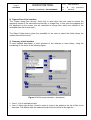
The “Graphical routines” for a given supported module can be started in command line
mode by typing:
<Module Code Name>_visu.exe xxx
The <Module Code Name> prefix will be one of the following:
•
‘medll‘ for MEDLL module
•
‘prediction‘ for Prediction Tool module
•
‘carrierphase‘ for Carrier Phase module
•
‘dynamics‘ for the Aircraft Dynamics module
•
‘procedure’ for the Procedure module
the ‘xxx’ input argument contains the path and file name of ‘ini’ file used by the module
without its extension. For example, in order to visualize the output of the Prediction module,
the user shall type in the command prompt:
‘prediction_visu.exe C:\data\prediction’
Where “C:\data\prediction.ini” is the ‘ini’ file used by the prediction module to generate its
output(s).
Project:
PEGASUS
EUROCONTROL
Issue:
Software User Manual – MFILERUNNER
3.3
Doc. No.:
Sheet
PEG-SUM-MFR
K
Date:
13 of 70
16/01/2004
Detailed Description of the Graphical Routines
3.3.1 SBAS Messages visualisation
The SBAS Visualisation module generates graphs for SBAS Messages analysis
containing Slow, Fast and Iono corrections together with SIS statistics.
The interface is separated in four main parts:
•
•
•
•
SBAS Fast Corrections analysis (includes time and statistics series cf. 4.1 and 4.4)
– analyses the PRN mask and evaluates the fast correction data. It will produce time
and statistics interactive plots for the PRC and the UDREI for the satellites that are
currently contained in the PRN-mask.
SBAS Slow Correction analysis (includes time and statistics series cf. 4.1 and 4.4) –
analyses the PRN mask and evaluates the slow correction data. It will produce time
and statistics interactive plots for the slow corrections (for both velocity codes) for
the satellites that are currently contained in the PRN-mask.
SBAS Iono Corrections - analyses the IGP mask and evaluates the vertical delays
and the GIVEI for the transmitted bands and block. It will produce time interactive
plots of the vertical delays and GIVEI per point (see chapter 4.9) and an area plot for
the whole geographic area (see chapter 4.7). Additionally, it will produce a graph of
the area with the currently supported/unsupported IGPs.
SBAS Message Distribution - analyses the quantity distribution, the time distribution
and the broadcast frequency of the messages. It will generate a table with the
number of broadcast messages and will display the message type distribution and
time difference plots(see chapter 4.10).
3.3.2 WinGSPAll visualisation
The WinGPSAll Visualisation module generates graphs for position solution, protection
levels, integrity and availability using data computed by the WinGPSAll module.
The interface is separated in five main parts:
•
•
•
•
•
Interactive Plots – including time series (cf. §4.1) visualising WinGPSAll module
output
Standford Plots – analyses the horizontal and vertical situation for integrity and
availability purposes. It will produce a graphic identical to the one which can be
achieved by the Stanford University approach
North-East error – analyses the horizontal position error on North-east basis
Time Series for Position error and Protection levels – analyses the position error and
protection level data on time basis. It will produce graphics of the horizontal and
vertical position error and of the horizontal and vertical protection levels.
Statistics series - analyses the position error and protection level data and produces
histograms of the relevant data.
EUROCONTROL
Project:
PEGASUS
Doc. No.:
Issue:
Software User Manual – MFILERUNNER
Sheet
PEG-SUM-MFR
K
Date:
14 of 70
16/01/2004
3.3.3 MEDLL visualisation
The MEDLL module generates per PRN timed data such as the Pseudorange error for
example. By launching the ‘medll_visu’ executable with the proper input argument, the
user will have multiple way to visualise and analyse the output data of the module:
•
•
•
•
Per PRN Time series (cf. §4.2): To visualise the MEDLL module output data
temporally.
Per PRN Statistics series (cf. §4.4) : To visualise the statistics (histograms, PDF
and CDF) of MEDLL module output data.
Color Sky Plots (cf. §4.5): To visualise the MEDLL module output data grouped in
Elevation/Azimuth bins.
Per PRN Sky Plots (cf. §4.6): To visualise the course of the satellites with regard to
the receiver (Elevation/Azimuth positions).
3.3.4 Prediction Tool visualisation
The Prediction Tool module generates multiple output data files. By launching the
‘prediction_visu’ executable with the proper input argument, the user will have multiple
way to visualise and analyse the output data of the module. The launched GUIs will
vary depending on the processing configuration (The output files will vary in number
and in format depending on the configuration contained in the ini file). Please refer to
Prediction Tool module Software User Manual for a description of the 3 three possible
computing modes: ‘Point’ mode, ‘Tracked’ mode, ‘Grid’ mode.
3.3.4.1 Point mode and Track mode
Please find below a list of launched GUI for this mode:
•
•
•
•
•
Time series (cf. §4.1): To visualise receiver position used by the “Prediction Tool”
module.
Per PRN Time series (cf. §4.2): To visualise “Prediction Tool” predicted value for
satellite information (position, velocity, etc).
Time series (cf. §4.1): To visualise “Prediction Tool” predicted value for DOP,
Protection levels, NSE, etc…
Statistics series (cf. §4.3) : To visualise the statistics (histograms, PDF and CDF) of
“Prediction Tool” predicted value (DOP, Protection levels, NSE, etc)
Per PRN Sky Plots (cf. §4.6): To visualise the course of the satellites with regard to
the receiver (Elevation/Azimuth positions).
Project:
PEGASUS
EUROCONTROL
Doc. No.:
Issue:
Software User Manual – MFILERUNNER
Sheet
PEG-SUM-MFR
K
Date:
15 of 70
16/01/2004
3.3.4.2 Grid mode
Please find below a list of launched GUI for this mode:
• Instantaneous Grid Plot Series (cf. §4.7): To visualise the instantaneous “Grid Plot”
of “Prediction Tool” predicted value (DOP, Protection levels, NSE, etc)
• Statistics Grid Plot Series (cf. §4.8): To visualise the “Grid Plot” of statistics for
“Prediction Tool” predicted value (DOP, Protection levels, NSE, etc)
3.3.5 Carrier Phase visualisation
The Carrier Phase module generates timed data such as the receiver antenna position
for example. By launching the ‘carrierphase_visu’ executable with the proper input
argument, the user will be able to visualise and analyse the output data of the module
with the “Time series” GUI (cf. §4.1).
3.3.6 Dynamics visualisation
The Dynamics module generates timed data such as the Navigation system error for
example. By launching the ‘dynamics_visu’ executable with the proper input argument,
the user will have multiple way to visualise and analyse the output data of the module:
• Time series (cf. §4.1): To visualise the Dynamics module output data temporally.
• Statistics series (cf. §4.3) : To visualise the statistics (histograms, PDF and CDF) of
the Dynamics module output data.
One to five additional figures might be generated depending on the configuration used
for the Dynamics module processing (defined in the ‘ini’ file):
•
•
•
•
•
three-dimensional plots of NSFP, AFP and DFP.
Procedure display with corresponding NSFP and AFP
Pressure versus height display
Temperature versus height display
Aircraft Dynamics display (Acceleration, Ground Speed and Attitude)
3.3.7 Procedure visualisation
Depending on the configuration contained in the ‘ini’ file one to three figures are
generated:
• Procedure display: always generated
• Message type 2 display: generated if message available
• Message type 4 display: generated if message available
All three figures does not require any interaction with the user.
EUROCONTROL
Project:
PEGASUS
Issue:
Software User Manual – MFILERUNNER
3.4
Doc. No.:
Sheet
PEG-SUM-MFR
K
Date:
16 of 70
16/01/2004
Operating Modes
All five module visualisation executables can be operated in two modes:
1. Embedded Mode:
The executables are run inside the PEGASUS frame via the M-file runner
module. This mode of operation is described in Error! Reference source not
found..
2. Command-line Mode:
The Graphical routines for a given supported module can be started in command
line mode by typing:
<Module Name>_visu.exe xxx
the ‘xxx’ input argument contains the path and file name of ‘ini’ file used by the
module without its extension. For example, in order to visualize the output of the
Prediction module, the user shall type in the command prompt:
‘ prediction_visu.exe C:\data\prediction ’
Where “C:\data\prediction.ini” is the ‘ini’ file used by the prediction module to
generate its output(s).
EUROCONTROL
Project:
PEGASUS
Doc. No.:
Issue:
Software User Manual – MFILERUNNER
Sheet
PEG-SUM-MFR
K
Date:
17 of 70
16/01/2004
4 Services
4.1
“Time series” Graphical Interface
The following section provides an overview of the graphical user interface of the “Time
series” GUI.
4.1.1
Main GUI
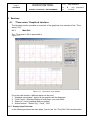
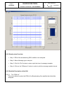
The “Time series” GUI is presented in
Figure 4.1-1.
Figure 4.1-1: “Time series” main window
From the main window 4 different parts can be seen:
1. “Graphics sub-window”: where all the graphics will be displayed
2. “Time Frame”: Selection/Display of time begin, end, and offset
3. “Data List”: List of available data for plotting
4. “Action buttons”: “Detach Fig”, “Clear”, “Plot”
4.1.2 Step-by-step Overview
In the following sections the main steps ‘how-to-use’ the “Time Plot” GUI are described.
Project:
PEGASUS
EUROCONTROL
Doc. No.:
Issue:
Software User Manual – MFILERUNNER
Sheet
PEG-SUM-MFR
K
Date:
18 of 70
16/01/2004
Step1: Select Data to plot
Single plot: select a data by clicking on its description in the “Data list” list box
Multiple subplots: hold the control key [Ctrl] and click on one or more data that you want
to plot in the “Data list” list box.
Step 2: Click On “Clear” button
A click on this button will delete all graphics in current GUI if any. This button will have
no effect if nothing is plotted yet.
Step 3: Click On “Plot” button
When you click on this button, the data you have selected in the first step will be
plotted as a function of time. See section 4.1.3.3 for more explanations on this feature.
Step 4: Click On “Detach Fig” button
Click on this button to “detach” the current plots from the GUI by creating a new figure.
See section 4.1.3.5 for more explanations on this feature.
Step 5: Save the figure
Click on the export menu to save the current figure in one of the proposed format. See
section 4.1.3.5 for more explanations on this feature.
4.1.3 Detailed Description of the GUI
4.1.3.1 The “Time frame”
This group of edit boxes and button allows to control the time windows that applies to
current plots. When edited, the user can change any of the following information:
• Beginning of GPS time (Week and Second edit boxes): The displayed time refers to
the time begin of the plot(s).
• End of GPS time (Week and Second edit boxes) :The displayed time refers to the time
end of the plot(s).
• Offset time (Second only edit box) : The displayed time refers to the time window
length in seconds. It is always equal to elapsed time between time begin and time
end.
To change any of these times, edit one of the five edit boxes and click on the “Plot” button or type [Enter] key
of your keyboard.
Remark 1: The Gregorian date/time above these edit boxes will automatically reflect
the time change.
Remark 2: The time displayed in the edit boxes are automatically updated to reflect any
change done manually by the user in one of the edit boxes.
The “Init” button permits to initialise the time window to the time begin and time end of
the original data.
EUROCONTROL
Project:
PEGASUS
Issue:
Software User Manual – MFILERUNNER
PEG-SUM-MFR
Doc. No.:
K
Sheet
Date:
19 of 70
16/01/2004
4.1.3.2 The “Data list frame”
This list box display a list of data available for plotting. The user can select more than
one data by pressing the [Ctrl] key before left-clicking with the mouse.
4.1.3.3 The “Plot” button
This button allows to plot the data selected in the “Data List” against the time window
displayed in the “Time Frame”.
Important Note:
• The number of subplots will be equal to the number of data selected.
Each time the user click on the plot button, the software will first check the current state
of the graphics sub-window:
If empty, the software will create one or more subplot depending on the selected data.
If not empty and if the current number of subplot is different from the number of data
selected, the software will erase the current subplot(s) before plotting the new one(s)
If not empty and if the current number of subplot is equal to the number of data
selected, the software will plot the new data onto current subplot(s) while conserving
current graphics.
4.1.3.4 The “Clear” button
This button deletes all the graphics of current GUI.
4.1.3.5 The “Detach Fig” button
This button allows all the graphics of current GUI to be copied onto a new figure. This
button should be used whenever the user is happy with the data displayed and wants to
save the results.
This new figure does not contain any user interface control but permits to manipulate
the graphics by means of the figure toolbar.
In addition the new figure contains some useful information about the displayed data in
an info box at the right of the graphics sub-window.
By clicking the export menu, the user can save the current figure in one of the proposed
format (a popup window allows to name the graphics file):
• Enhanced Windows Metafile (‘emf’ extension)
• 256 colours Windows Bitmap (‘bmp’ extension)
• JPEG image (‘jpg’ extension)
• PNG image (‘png’ extension)
• PDF format (‘pdf’ extension)
• Encapsulated Postscript (‘eps’ extension)
By clicking the copy menu, the user can copy the current figure:
• to Clipboard in Metafile format,
Project:
PEGASUS
EUROCONTROL
Doc. No.:
Issue:
Software User Manual – MFILERUNNER
• to Clipboard in Bitmap format,
• to Current Printer in color,
• to Current Printer in monochrome,
• to Selected Printer.
Sheet
PEG-SUM-MFR
K
Date:
20 of 70
16/01/2004
EUROCONTROL
Project:
PEGASUS
Issue:
Software User Manual – MFILERUNNER
4.2
PEG-SUM-MFR
Doc. No.:
K
Sheet
Date:
21 of 70
16/01/2004
“Per PRN Time series” Graphical Interface
The following section provides an overview of the graphical user interface of the “Per
PRN Time series” GUI. This GUI differs from the “Time series” one in that the user can
select the data he wants to plot on a per PRN basis. This implies that multiple data
cannot be plotted in the same subplot.
4.2.1
Main GUI
The “Per PRN Time series” GUI is presented in Figure 4.2-1.
Figure 4.2-1: “Per PRN Time series” main window
From the main window the 5 different parts can be seen:
1. “Graphics sub-window”: where all the graphics will go
2. “Time Frame”: Selection/Display of time begin, end, and offset
3. “Data List Frame: List of available data for plotting
4. “PRN List Frame”: List of available PRN for plotting
5. Action buttons: “Detach Fig”, “Plot”
4.2.2 Step-by-step Overview
In the following sections the main steps ‘how-to-use’ the “Per PRN Time Plot” GUI are
described:
Project:
PEGASUS
EUROCONTROL
Doc. No.:
Issue:
Software User Manual – MFILERUNNER
Sheet
PEG-SUM-MFR
K
Date:
22 of 70
16/01/2004
•
Step 1: Select Data to plot
• Single plot: select a data by clicking on its description in the “Data list” list
box
• Multiple subplots: hold the control key [Ctrl] and click one or more time on
the data you want to plot in the “Data list” list box.
•
Step 2: Select PRN(s) to plot
• Single PRN: select a PRN by clicking on it in the “PRN list” list box
• Multiple PRN: hold the control key [Ctrl] and click one or more time on the
PRN(s) you want to plot in the “PRN list” list box.
• All PRN: click on the “All PRN” check box.
•
Step 3: Click On “Plot” button
When you click on this button, the data you have selected in the first step will
be plotted as a function of time for all selected PRN (in step 2).
•
Step 4: Click On “Detach Fig” button
Click on this button to “detach” the current plots from the GUI by creating a new
figure.
•
Step 5: Save the figure
Click on the export menu to save the current figure in one of the proposed
format.
4.2.3 Detailed Description of the GUI
4.2.3.1 The “Time frame”
This group of edit boxes and button allows to control the time windows that applies to
current plots. When edited, the user can change any of the following information:
• Beginning of GPS time (Week and Second edit boxes): The displayed time refers to
the time begin of the plot(s).
• End of GPS time (Week and Second edit boxes) :The displayed time refers to the time
end of the plot(s).
• Offset time (Second only edit box) : The displayed time refers to the time window
length in seconds. It is always equal to elapsed time between time begin and time
end.
To change any of these times, edit one of the five edit boxes and click on the “Plot” button or type [Enter] key
of your keyboard.
Remark 1: The Gregorian date/time above these edit boxes will automatically reflect
the time change.
Remark 2: The time displayed in the edit boxes are automatically updated to reflect any
change done manually by the user in one of the edit boxes.
EUROCONTROL
Project:
PEGASUS
Doc. No.:
Issue:
Software User Manual – MFILERUNNER
Sheet
PEG-SUM-MFR
K
Date:
23 of 70
16/01/2004
The “Init” button permits to initialise the time window to the time begin and time end of
the original data.
4.2.3.2 The “Data list frame”
This list box display a list of data available for plotting. The user can select more than
one data by pressing the [Ctrl] key before left-clicking with the mouse.
4.2.3.3 The “PRN list frame”
The user can choose here the PRN for which he wants to analyse the Data selected in the
“Data list frame”.
The check-box “Use All PRN” allows to select all the PRN displayed in the list box in one
go.
4.2.3.4 The “Plot” button
This button allows to plot the data selected in the “Data List” for the PRN selected in the
“PRN list frame” against the time window displayed in the “Time Frame”.
Important Notes:
• The number of subplots will be equal to the number of data selected. All previous
graphics will be deleted.
• The number of curves will be equal to the number of PRN selected in the “PRN list
frame”.
4.2.3.5 The “Detach Fig” button
This button allows all the graphics of current GUI to be copied onto a new figure. This
button should be used whenever the user is happy with the data displayed and wants to
save the results.
This new figure does not contain any user interface control but permits to manipulate
the graphics by means of the figure toolbar.
In addition the new figure contains some useful information about the displayed data in
an info box at the right of the graphics sub-window.
By clicking the export menu, the user can save the current figure in one of the proposed
format (a popup window allows to name the graphics file):
• Enhanced Windows Metafile (‘emf’ extension)
• 256 colours Windows Bitmap (‘bmp’ extension)
• JPEG image (‘jpg’ extension)
• PNG image (‘png’ extension)
• PDF format (‘pdf’ extension)
• Encapsulated Postscript (‘eps’ extension)
By clicking the copy menu, the user can copy the current figure:
Project:
PEGASUS
EUROCONTROL
Doc. No.:
Issue:
Software User Manual – MFILERUNNER
• to Clipboard in Metafile format,
• to Clipboard in Bitmap format,
• to Current Printer in color,
• to Current Printer in monochrome,
• to Selected Printer.
Sheet
PEG-SUM-MFR
K
Date:
24 of 70
16/01/2004
EUROCONTROL
Project:
PEGASUS
Issue:
Software User Manual – MFILERUNNER
4.3
Doc. No.:
Sheet
PEG-SUM-MFR
K
Date:
25 of 70
16/01/2004
“Statistics series” Graphical Interface
This section provides an overview of the graphical user interface of the “Statistics
series” GUI. This GUI differs from the “Time series” in that the data is not simply
displayed as a function of time. Instead, the statistical properties of the data are
analysed and three types of plot are offered to the user: histograms, PDF and CDF. The
following section will help the user understanding the workings of this GUI.
4.3.1
Main GUI
The “Statistics series” GUI is presented in
Figure 4.3-1.
Figure 4.3-1: “Statistics series” main window
From the main window the 5 different parts can be seen:
1. “Graphics sub-window”: where all the graphics will go
2. “Time Frame”: Selection/Display of time begin, end, and offset
3. “Data List”: List of available data for processing and display
4. “Action Frame”: Selection of Statistics Type and Action buttons (“Detach Fig”,
“Clear”, “Plot”)
5. “Desired Probability Frame”: Set and search desired Probability, this frame is not
always visible (c.f. §4.3.3.8).
EUROCONTROL
Project:
PEGASUS
Doc. No.:
Issue:
Software User Manual – MFILERUNNER
Sheet
PEG-SUM-MFR
K
Date:
26 of 70
16/01/2004
4.3.2 Step-by-step Overview
In the following sections the main steps ‘how-to-use’ the “Statistics series” GUI are
described:
•
Step 1: Select Data to analyse for statistics plot.
• Single plot: select a data by clicking on its description in the “Data list” list
box.
• Multiple subplots: hold the control key [Ctrl] and click one or more time on
the data you want to plot in the “Data list” list box.
•
Step 2: Click On “Clear” button
A click on this button will delete all graphics in current GUI if any. This button
will have no effect if there is nothing plotted yet.
•
Step 3: Select type of statistics
• Histogram: right-click on “Histogram” radio-button
• PDF: right-click on “Probability Density Function” radio-button
• CDF: right-click on “Cumulative Density Function” radio-button
•
Step 4: Click On “Plot” button
When you click on this button, depending on what type of statistics you selected
in the previous step, histogram(s), PDF(s) or CDF(s) of the data selected in the
first step will be plotted.
•
Step 5: Click On “Detach Fig” button
Click on this button to “detach” the current plots from the GUI by creating a new
figure.
•
Step 6: Save the figure
Click on the export menu to save the current figure in one of the proposed
format.
4.3.3 Detailed Description of the GUI
4.3.3.1 The “Time frame”
This group of edit boxes and button allows to control the time windows that applies to
current plots. When edited, the user can change any of the following information:
• Beginning of GPS time (Week and Second edit boxes): The displayed time refers to
the time begin of the plot(s).
• End of GPS time (Week and Second edit boxes) :The displayed time refers to the time
end of the plot(s).
• Offset time (Second only edit box) : The displayed time refers to the time window
length in seconds. It is always equal to elapsed time between time begin and time
end.
EUROCONTROL
Project:
PEGASUS
Doc. No.:
Issue:
Software User Manual – MFILERUNNER
Sheet
PEG-SUM-MFR
K
Date:
27 of 70
16/01/2004
To change any of these times, edit one of the five edit boxes and click on the “Plot”
button or type [Enter] key of your keyboard.
Remark 1: The Gregorian date/time above these edit boxes will automatically reflect
the time change.
Remark 2: The time displayed in the edit boxes are automatically updated to reflect any
change done manually by the user in one of the edit boxes.
The “Init” button permits to initialise the time window to the time begin and time end of
the original data.
4.3.3.2 The “Data list frame”
This list box display a list of data available for plotting. The user can select more than
one data by pressing the [Ctrl] key before left-clicking with the mouse.
4.3.3.3 The “Statistics Type” radio-buttons
Right-click on the radio-button of your choice to select histograms, PDF (Probability
Density Function) or CDF (Cumulative Density Function).
4.3.3.4 The “Number of bins” edit box
This edit box allows the user to change the number of bins used for statistics
calculation. To change this value, right-click on it and type in the value you want. To
validate this new number of bins, right-click on the “Plot” button or type [Enter] key of
your keyboard.
4.3.3.5 The “Plot” button
This button allows to plot statistics for the data selected in the “Data List”. The number
of subplots will be equal to the number of data selected. All previous graphics
will be deleted.
The statistics are calculated with the displayed “number of bins” just before being
plotted. Only the subset of data corresponding to the time window displayed in the
“Time Frame” will be used for the calculation.
Each time the user click on the plot button, the software will first check the current state
of the graphics sub-window:
If empty, the software will create one or more subplot depending on the selected data.
If not empty and if the current number of subplot is different from the number of data
selected, the software will erase the current subplot(s) before plotting the new one(s)
If not empty and if the current number of subplot is equal to the number of data
selected, the software will plot the new data onto current subplot(s) while conserving
current graphics.
Project:
PEGASUS
EUROCONTROL
Doc. No.:
Issue:
Software User Manual – MFILERUNNER
Sheet
PEG-SUM-MFR
K
Date:
28 of 70
16/01/2004
4.3.3.6 The “Clear” button
This button deletes all the graphics of current GUI.
4.3.3.7 The “Detach Fig” button
This button allows all the graphics of current GUI to be copied onto a new figure. This
button should be used whenever the user is happy with the data displayed and wants to
save the results.
This new figure does not contain any user interface control but permits to manipulate
the graphics by means of the figure toolbar.
In addition the new figure contains some useful information about the displayed data in
an info box at the right of the graphics sub-window.
By clicking the export menu, the user can save the current figure in one of the proposed
format (a popup window allows to name the graphics file):
• Enhanced Windows Metafile (‘emf’ extension)
• 256 colours Windows Bitmap (‘bmp’ extension)
• JPEG image (‘jpg’ extension)
• PNG image (‘png’ extension)
• PDF format (‘pdf’ extension)
• Encapsulated Postscript (‘eps’ extension)
By clicking the copy menu, the user can copy the current figure:
• to Clipboard in Metafile format,
• to Clipboard in Bitmap format,
• to Current Printer in color,
• to Current Printer in monochrome,
• to Selected Printer.
4.3.3.8 The “Desired Probability” frame
This frame allows the user to search for a desired probability for all the curves plotted in
the “Graphics” sub-window. This frame is only visible in the “Statistics Type” is set
to “Cumulative Density Function” (c.f. §4.3.3.3). The frame is composed of :
•
an edit box to input the desired probability
Any value between 0 and 1 is allowed.
•
a search button to search for the desired probability
A right-click on this button will search for the value displayed in the edit box
above in all the curves plotted in the “Graphics” sub-window. It will also draw
some line and circles to show found values (see
Figure 4.1-1).
•
a clear button to clear all the texts and lines drawn by the search button.
EUROCONTROL
Project:
PEGASUS
Issue:
Software User Manual – MFILERUNNER
4.4
Doc. No.:
Sheet
PEG-SUM-MFR
K
Date:
29 of 70
16/01/2004
“Per PRN Statistics series” Graphical Interface
The following section provides an overview of the graphical user interface of the “Per
PRN Statistics series” GUI. This GUI differs from the “per PRN Time series” in that the
data is not simply displayed as a function of time. Instead, the statistical properties of
the data is analysed and three type of plot are offered to the user: histograms, PDF and
CDF. This GUI differs from the “Statistics series” one in that the user can select the
data he wants to analyse statistics for on a per PRN basis. This implies that multiple
data cannot be plotted in the same subplot.
4.4.1
Main GUI
The “Statistics series” GUI is presented in Figure 4.4-1.
Figure 4.4-1: “Per PRN Statistics series” main window
From the main window the 5 different parts can be seen:
“Graphics sub-window”: where all the graphics will go
“Time Frame”: Selection/Display of time begin, end, and offset
“Data List”: List of available data for processing and display
“Action Frame”: Selection of Statistics Type and Action buttons (“Detach Fig”, “Clear”,
“Plot”)
EUROCONTROL
Project:
PEGASUS
Doc. No.:
Issue:
Software User Manual – MFILERUNNER
Sheet
PEG-SUM-MFR
K
Date:
30 of 70
16/01/2004
“Desired Probability Frame”: Set and search desired Probability, this frame is not
always visible (c.f. §4.4.3.9).
4.4.2 Step-by-step Overview
In the following sections the main steps ‘how-to-use’ the “Statistics series” GUI are
described:
•
Step 1: Select Data to analyse for statistics plot.
• Single plot: select a data by clicking on its description in the “Data list” list
box.
• Multiple subplots: hold the control key [Ctrl] and click one or more time on
the data you want to plot in the “Data list” list box.
•
Step 2: Select PRN(s) to plot
• Single PRN: select a PRN by clicking on it in the “PRN list” list box
• Multiple PRN: hold the control key [Ctrl] and click one or more time on the
PRN(s) you want to plot in the “PRN list” list box.
• All PRN: click on the “All PRN” check box.
•
Step 3: Select type of statistics
• Histogram: right-click on “Histogram” radio-button
• PDF: right-click on “Probability Density Function” radio-button
• CDF: right-click on “Cumulative Density Function” radio-button
•
Step 4: Click On “Plot” button
When you right-click on this button, depending on what type of statistics you
selected in the previous step, histogram(s), PDF(s) or CDF(s) of the data
selected in the first step will be plotted.
•
Step 5: Click On “Detach Fig” button
Right-Click on this button to “detach” the current plots from the GUI by creating
a new figure.
•
Step 6: Save the figure
Right-Click on the export menu to save the current figure in one of the proposed
format.
4.4.3 Detailed Description of the GUI
4.4.3.1 The “Time frame”
This group of edit boxes and button allows to control the time windows that applies to
current plots. When edited, the user can change any of the following information:
• Beginning of GPS time (Week and Second edit boxes): The displayed time refers to
the time begin of the plot(s).
EUROCONTROL
Project:
PEGASUS
Doc. No.:
Issue:
Software User Manual – MFILERUNNER
Sheet
PEG-SUM-MFR
K
Date:
31 of 70
16/01/2004
• End of GPS time (Week and Second edit boxes) :The displayed time refers to the time
end of the plot(s).
• Offset time (Second only edit box) : The displayed time refers to the time window
length in seconds. It is always equal to elapsed time between time begin and time
end.
To change any of these times, edit one of the five edit boxes and click on the “Plot”
button or type [Enter] key of your keyboard.
Remark 1: The Gregorian date/time above these edit boxes will automatically reflect
the time change.
Remark 2: The time displayed in the edit boxes are automatically updated to reflect any
change done manually by the user in one of the edit boxes.
The “Init” button permits to initialise the time window to the time begin and time end of
the original data.
4.4.3.2 The “Data list frame”
This list box display a list of data available for plotting. The user can select more than
one data by pressing the [Ctrl] key before left-clicking with the mouse.
4.4.3.3 The “PRN list frame”
The user can choose here the PRN for which he wants to analyse the Data selected in
the “Data list frame”.
The check-box “Use All PRN” allows to select all the PRN displayed in the list box in
one go.
4.4.3.4 The “All PRN as one” toggle button
When this toggle button is set (by right-clicking on it), the PRN selected in the “PRN list
frame” will be grouped for each data selected in the “Data list frame”. Then the new “All
PRN as one” data will be used for the calculation.
4.4.3.5 The “Statistics Type” radio-buttons
A right-click on one of the three radio-buttons allows the user to select histograms, PDF
(Probability Density Function) or CDF (Cumulative Density Function).
4.4.3.6 The “Number of bins” edit box
This edit box allows the user to change the number of bins used for statistics
calculation. To change this value, right-click on it and type in the value you want. To
validate this new number of bins, right-click on the “Plot” button or type [Enter] key of
your keyboard.
Project:
PEGASUS
EUROCONTROL
Doc. No.:
Issue:
Software User Manual – MFILERUNNER
Sheet
PEG-SUM-MFR
K
Date:
32 of 70
16/01/2004
4.4.3.7 The “Plot” button
This button allows to plot statistics for the data selected in the “Data List” and the PRN
selected in the “PRN list frame”.
Important Notes:
• The number of subplots will be equal to the number of data selected. All previous
graphics will be deleted.
• If “All PRN as One” toggle button is set, the number of curves will be equal to the
number of PRN selected in the “PRN list frame”, else there will be only one curve.
The statistics are calculated with the displayed “number of bins” just before being
plotted. Only the subset of data corresponding to the time window displayed in the
“Time Frame” and the PRN selected in the “PRN list frame” will be used for the
calculation.
4.4.3.8 The “Detach Fig” button
This button allows all the graphics of current GUI to be copied onto a new figure. This
button should be used whenever the user is happy with the data displayed and wants to
save the results.
This new figure does not contain any user interface control but permits to manipulate
the graphics by means of the figure toolbar.
In addition the new figure contains some useful information about the displayed data in
an info box at the right of the graphics sub-window.
By clicking the export menu, the user can save the current figure in one of the proposed
format (a popup window allows to name the graphics file):
• Enhanced Windows Metafile (‘emf’ extension)
• 256 colours Windows Bitmap (‘bmp’ extension)
• JPEG image (‘jpg’ extension)
• PNG image (‘png’ extension)
• PDF format (‘pdf’ extension)
• Encapsulated Postscript (‘eps’ extension)
By clicking the copy menu, the user can copy the current figure:
• to Clipboard in Metafile format,
• to Clipboard in Bitmap format,
• to Current Printer in color,
• to Current Printer in monochrome,
• to Selected Printer.
Project:
PEGASUS
EUROCONTROL
Doc. No.:
Issue:
Software User Manual – MFILERUNNER
Sheet
PEG-SUM-MFR
K
Date:
33 of 70
16/01/2004
4.4.3.9 The “Desired Probability” frame
This frame allows the user to search for a desired probability for all the curves plotted in
the “Graphics” sub-window. This frame is only visible in the “Statistics Type” is set
to “Cumulative Density Function” (c.f. §4.4.3.4). The frame is composed of :
•
an edit box to input the desired probability
Any value between 0 and 1 is allowed.
•
a search button to search for the desired probability
A right-click on this button will search for the value displayed in the edit box
above in all the curves plotted in the “Graphics” sub-window. It will also draw
some line and circles to show found values (see
Figure 4.1-1).
•
a clear button to clear all the texts and lines drawn by the search button.
EUROCONTROL
Project:
PEGASUS
Issue:
Software User Manual – MFILERUNNER
4.5
Doc. No.:
Sheet
PEG-SUM-MFR
K
Date:
34 of 70
16/01/2004
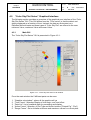
“Color Sky Plot Series” Graphical Interface
The following section provides an overview of the graphical user interface of the “Color
Sky Plot Series” GUI. This GUI differs from the “Time series” in that the data is not
simply displayed as a function of time. Instead, the data are first sorted on a
Elevation/Azimuth basis and three types of “Color Sky Plot” are offered to the user:
minimum Value, maximum Value and mean Value.
4.5.1
Main GUI
The “Color Sky Plot Series” GUI is presented in Figure 4.5-1.
Figure 4.5-1: “Color Sky Plot series” main window
From the main window the 5 different parts can be seen:
1.
2.
3.
4.
5.
“Graphics sub-window”: where all the graphics will go
“Time Frame”: Selection/Display of time begin, end, and offset
“Data List”: List of available data for processing and display
“Action Frame”: Selection of Plot Type and Action buttons (“Detach Fig”, “Plot”)
“Range Frame”: Set or Initialise minimum and maximum values for current plots.
EUROCONTROL
Project:
PEGASUS
Issue:
Software User Manual – MFILERUNNER
PEG-SUM-MFR
Doc. No.:
K
Sheet
Date:
35 of 70
16/01/2004
4.5.2 Step-by-step Overview
In the following sections the main steps ‘how-to-use’ the “Color Sky Plot Series” GUI
are described:
•
Step 1: Select Data to analyse for statistics plot.
• Single plot: select a data by clicking on its description in the “Data list” list
box.
• Multiple subplots: hold the control key [Ctrl] and click one or more time on
the data you want to plot in the “Data list” list box.
•
Step 2: Click On “Clear” button
A click on this button will delete all graphics in current GUI if any. This button
will have no effect if there is nothing plotted yet.
•
Step 3: Select type of “Color Sky Plot”
• Minimum value: minimum value of the data will be plotted
• Maximum value: maximum value of the data will be plotted
• Mean value: mean value of the data will be plotted
•
Step 4: Click On “Plot” button
When you click on this button, depending on what type of statistics you selected
in the previous step, minimum “Color Sky plot(s)”, “maximum Color Sky plot(s)”
or “mean Color Sky plot(s)” of the data selected in the first step will be plotted.
•
Step 5: Click On “Detach Fig” button
Click on this button to “detach” the current plots from the GUI by creating a new
figure.
•
Step 6: Save the figure
Click on the export menu to save the current figure in one of the proposed
format.
EUROCONTROL
Project:
PEGASUS
Doc. No.:
Issue:
Software User Manual – MFILERUNNER
Sheet
PEG-SUM-MFR
K
Date:
36 of 70
16/01/2004
4.5.3 Detailed Description of the GUI
4.5.3.1 The “Time frame”
This group of edit boxes and button allows to control the time windows that applies to
current plots. When edited, the user can change any of the following information:
• Beginning of GPS time (Week and Second edit boxes): The displayed time refers to
the time begin of the plot(s).
• End of GPS time (Week and Second edit boxes) :The displayed time refers to the time
end of the plot(s).
• Offset time (Second only edit box) : The displayed time refers to the time window
length in seconds. It is always equal to elapsed time between time begin and time
end.
To change any of these times, edit one of the five edit boxes and click on the “Plot” button or type [Enter] key
of your keyboard.
Remark 1: The Gregorian date/time above these edit boxes will automatically reflect
the time change.
Remark 2: The time displayed in the edit boxes are automatically updated to reflect any
change done manually by the user in one of the edit boxes.
The “Init” button permits to initialise the time window to the time begin and time end of
the original data.
4.5.3.2 The “Data list frame”
This list box display a list of data available for plotting. The user can select more than
one data by pressing the [Ctrl] key before left-clicking with the mouse.
4.5.3.3 The “Plot Type” radio-buttons
Right-click on the radio-button of your choice to select minimum Color Sky plot,
maximum Color Sky plot or mean Color Sky plot.
4.5.3.4 The “Plot” button
This button allows to Color Sky Plot(s) for the data selected in the “Data List”.
Important Notes:
• The number of subplots will be equal to the number of data selected. All previous
graphics will be deleted.
• Only the subset of data corresponding to the time window displayed in the “Time
Frame” will be used for the calculation.
EUROCONTROL
Project:
PEGASUS
Doc. No.:
Issue:
Software User Manual – MFILERUNNER
Sheet
PEG-SUM-MFR
K
Date:
37 of 70
16/01/2004
4.5.3.5 The “Detach Fig” button
This button allows all the graphics of current GUI to be copied onto a new figure. This
button should be used whenever the user is happy with the data displayed and wants to
save the results.
This new figure does not contain any user interface control but permits to manipulate
the graphics by means of the figure toolbar.
In addition the new figure contains some useful information about the displayed data in
an info box at the right of the graphics sub-window.
By clicking the export menu, the user can save the current figure in one of the proposed
format (a popup window allows to name the graphics file):
• Enhanced Windows Metafile (‘emf’ extension)
• 256 colours Windows Bitmap (‘bmp’ extension)
• JPEG image (‘jpg’ extension)
• PNG image (‘png’ extension)
• PDF format (‘pdf’ extension)
• Encapsulated Postscript (‘eps’ extension)
By clicking the copy menu, the user can copy the current figure:
• to Clipboard in Metafile format,
• to Clipboard in Bitmap format,
• to Current Printer in color,
• to Current Printer in monochrome,
• to Selected Printer.
4.5.3.6 The “Range frame”
This frame allows the user to fix minimum and maximum values for the Sky Plots
currently under display.
The frame is composed of :
•
•
•
•
•
a “MIN” edit box to input the minimum desired value.
a “MAX” edit box to input the maximum desired value.
an “Apply” button to apply minimum and/or maximum value currently displayed in
the “MIN” and “MAX” edit boxes.
a “Keep” toggle button to force any new plot to use current range values.
an “Init” button to initialise “MIN” and “MAX” edit boxes to the true minimum and
maximum values of the currently selected data.
EUROCONTROL
Project:
PEGASUS
Issue:
Software User Manual – MFILERUNNER
4.6
Doc. No.:
Sheet
PEG-SUM-MFR
K
Date:
38 of 70
16/01/2004
“Per PRN Sky Plot Series” Graphical Interface
The following section provides an overview of the graphical user interface of the “Per
PRN Sky Plot Series” GUI. This GUI allows the user to plot satellite position (i.e.
Elevation/Azimuth) with regard to the receiver for a certain time windows.
4.6.1
Main GUI
The “Per PRN Sky Plot Series” GUI is presented in Figure 4.6-1.
Figure 4.6-1: “Per PRN Sky Plot series” main window
From the main window the 4 different parts can be seen:
1. “Graphics sub-window”: where all the graphics will go
2. “Time Frame”: Selection/Display of time begin, end, and offset
3. “PRN List”: List of available data for processing and display
4.
“Action Frame”: “Detach Fig” and “Plot” buttons
4.6.2 Step-by-step Overview
In the following sections the main steps ‘how-to-use’ the “Per PRN Sky Plottings” GUI are described:
EUROCONTROL
Project:
PEGASUS
Doc. No.:
Issue:
Software User Manual – MFILERUNNER
Sheet
PEG-SUM-MFR
K
Date:
39 of 70
16/01/2004
•
Step 1: Select PRN for “Sky plots”.
•
Step 2: Click On “Plot” button
“Sky Plot” of each selected PRN will be plotted.
•
Step 3: Click On “Detach Fig” button
Click on this button to “detach” the current plots from the GUI by creating a new
figure.
•
Step 4: Save the figure
Click on the export menu to save the current figure in one of the proposed
format.
4.6.3 Detailed Description of the GUI
4.6.3.1 The “Time frame”
This group of edit boxes and button allows to control the time windows that applies to
current plots. When edited, the user can change any of the following information:
• Beginning of GPS time (Week and Second edit boxes): The displayed time refers to
the time begin of the plot(s).
• End of GPS time (Week and Second edit boxes) :The displayed time refers to the time
end of the plot(s).
• Offset time (Second only edit box) : The displayed time refers to the time window
length in seconds. It is always equal to elapsed time between time begin and time
end.
To change any of these times, edit one of the five edit boxes and click on the “Plot” button or type [Enter] key
of your keyboard.
Remark 1: The Gregorian date/time above these edit boxes will automatically reflect
the time change.
Remark 2: The time displayed in the edit boxes are automatically updated to reflect any
change done manually by the user in one of the edit boxes.
The “Init” button permits to initialise the time window to the time begin and time end of
the original data.
4.6.3.2 The “PRN list frame”
The user can choose here the PRN for which he wants to analyse the Data selected in
the “Data list frame”.
The check-box “Use All PRN” allows to select all the PRN displayed in the list box in
one go.
Project:
PEGASUS
EUROCONTROL
Doc. No.:
Issue:
Software User Manual – MFILERUNNER
Sheet
PEG-SUM-MFR
K
Date:
40 of 70
16/01/2004
4.6.3.3 The “Plot” button
This button allows to plot “Sky Plot(s)” for each selected PRN.
Important Note:
• Only the subset of data corresponding to the time window displayed in the “Time
Frame” will be used for the calculation.
4.6.3.4 The “Detach Fig” button
This button allows all the graphics of current GUI to be copied onto a new figure. This
button should be used whenever the user is happy with the data displayed and wants to
save the results.
This new figure does not contain any user interface control but permits to manipulate
the graphics by means of the figure toolbar.
In addition the new figure contains some useful information about the displayed data in
an info box at the right of the graphics sub-window.
By clicking the export menu, the user can save the current figure in one of the proposed
format (a popup window allows to name the graphics file):
• Enhanced Windows Metafile (‘emf’ extension)
• 256 colours Windows Bitmap (‘bmp’ extension)
• JPEG image (‘jpg’ extension)
• PNG image (‘png’ extension)
• PDF format (‘pdf’ extension)
• Encapsulated Postscript (‘eps’ extension)
By clicking the copy menu, the user can copy the current figure:
• to Clipboard in Metafile format,
• to Clipboard in Bitmap format,
• to Current Printer in color,
• to Current Printer in monochrome,
• to Selected Printer.
EUROCONTROL
Project:
PEGASUS
Issue:
Software User Manual – MFILERUNNER
4.7
PEG-SUM-MFR
Doc. No.:
K
Sheet
Date:
41 of 70
16/01/2004
“Instantaneous Grid Plot Series” Graphical Interface
The following section provides an overview of the graphical user interface of the
“Instantaneous Grid Plot Series” GUI. This GUI differs from the “Time series” in that the
data is not simply plotted as a function of time. Instead, the data are plotted as a
function of the receiver horizontal position (Latitude/Longitude) for a given time.
4.7.1
Main GUI
The “Instantaneous Grid Plot Series” GUI is presented in Figure 4.7-1.
Figure 4.7-1: “Instantaneous Grid Plot Series” GUI main window
From the main window the 5 different parts can be seen:
1. “Graphics sub-window”: where all the graphics will go
2. “Time Frame”: Selection of time of application
3. “Data List”: List of available data for processing and display
4. “Action Frame”: Action buttons (“Detach Fig”, “Plot”) and Selection of Plot Type
5.
“Range Frame”: Set or Initialise minimum and maximum values for current plots.
EUROCONTROL
Project:
PEGASUS
Doc. No.:
Issue:
Software User Manual – MFILERUNNER
Sheet
PEG-SUM-MFR
K
Date:
42 of 70
16/01/2004
4.7.2 Step-by-step Overview
In the following sections the main steps ‘how-to-use’ the “Instantaneous Grid Plot
Series” GUI are described:
•
Step 1: Select Data to analyse for statistics plot.
•
Step 2: Click on “Plot” button
When you right-click on this button the “Instantaneous Grid Plot” of the data
selected in the first step will be plotted. The time of application is displayed in
the “Time frame”.
•
Step 3: Click on the “Interpolated shading” check box
This will change the grid plot aspect to an interpolated shading.
•
Step 4: Change the time of application
Right-click on the right or left arrow of the “Time frame slider” to navigate the
“Grid Plot” chronologically.
•
Step 5: Click on “Detach Fig” button
Click on this button to “detach” the current plots from the GUI by creating a new
figure.
•
Step 6: Save the figure
Click on the export menu to save the current figure in one of the proposed
format.
4.7.3 Detailed Description of the GUI
4.7.3.1 The “Time frame”
The “Time frame” allows the user to change the time of application of the
“Instantaneous Grid Plot” currently under display.
This frame is composed of:
• two edit boxes to let the user input GPS time (Week and Sec) manually,
• a “time slider” to move the time chronologically,
• a “date/time text” to display the current Gregorian data/time.
All components all linked to provide consistent display for each user operation on the UI
controls.
4.7.3.2 The “Data list frame”
This is a pop-up menu allowing the user to select one data for “Instantaneous Grid
Plotting”.
EUROCONTROL
Project:
PEGASUS
Doc. No.:
Issue:
Software User Manual – MFILERUNNER
Sheet
PEG-SUM-MFR
K
Date:
43 of 70
16/01/2004
4.7.3.3 The “Plot” button
This button allows to “Instantaneous Grid Plot” for the data selected in the “Data List
frame” and the time of application displayed in the “Time frame”.
4.7.3.4 The “Detach Fig” button
This button allows all the graphics of current GUI to be copied onto a new figure. This
button should be used whenever the user is happy with the data displayed and wants to
save the results.
This new figure does not contain any user interface control but permits to manipulate
the graphics by means of the figure toolbar.
In addition the new figure contains some useful information about the displayed data in
an info box at the right of the graphics sub-window.
By clicking the export menu, the user can save the current figure in one of the proposed
format (a popup window allows to name the graphics file):
• Enhanced Windows Metafile (‘emf’ extension)
• 256 colours Windows Bitmap (‘bmp’ extension)
• JPEG image (‘jpg’ extension)
• PNG image (‘png’ extension)
• PDF format (‘pdf’ extension)
• Encapsulated Postscript (‘eps’ extension)
By clicking the copy menu, the user can copy the current figure:
• to Clipboard in Metafile format,
• to Clipboard in Bitmap format,
• to Current Printer in color,
• to Current Printer in monochrome,
• to Selected Printer.
4.7.3.5 The “Range frame”
This frame allows the user to fix minimum and maximum values for the Sky Plots
currently under display.
The frame is composed of :
•
•
•
•
•
a “MIN Value” edit box to input the minimum desired value.
a “MAX Value” edit box to input the maximum desired value.
an “Apply” button to apply minimum and/or maximum value currently displayed in
the “MIN” and “MAX” edit boxes.
a “Keep” toggle button to force any new plot to use current range values.
an “Init” button to initialise “MIN” and “MAX” edit boxes to the true minimum and
maximum values of the currently selected data.
EUROCONTROL
Project:
PEGASUS
Issue:
Software User Manual – MFILERUNNER
4.8
Doc. No.:
Sheet
PEG-SUM-MFR
K
Date:
44 of 70
16/01/2004
“Statistics Grid Plot Series” Graphical Interface
The following section provides an overview of the graphical user interface of the
“Statistics Grid Plot Series” GUI. This GUI differs from the “Instantaneous Grid Plot
series” in that it is independent of time. This GUI has been designed to visualise the
“GBAS-MARS 2 Prediction Tool” module statistics output.
4.8.1
Main GUI
The “Statistics Grid Plot Series” GUI is presented in Figure 4.8-1.
Figure 4.8-1: “Statistics Grid Plot Series” GUI main window
From the main window the 5 different parts can be seen:
1. “Graphics sub-window”: where all the graphics will go
2. “Data List”: List of available data for processing and display
3. “Statistics Type frame”: List of available statistics for grid plotting.
4. “Action Frame”: Action buttons (“Detach Fig”, “Plot”) and Selection of Plot Type
5.
“Range Frame”: Set or Initialise minimum and maximum values for current plots.
EUROCONTROL
Project:
PEGASUS
Doc. No.:
Issue:
Software User Manual – MFILERUNNER
Sheet
PEG-SUM-MFR
K
Date:
45 of 70
16/01/2004
4.8.2 Step-by-step Overview
In the following sections the main steps ‘how-to-use’ the “Instantaneous Grid Plot
Series” GUI are described:
•
Step 1: Select Data to analyse for statistics plot.
•
Step 2: Select type of “Statistics Grid Plot”
•
Step 3: Click On “Plot” button
When you right-click on this button the “Instantaneous Grid Plot” of the data
selected in the first step will be plotted. The time of application is displayed in
the “Time frame”.
•
Step 4: Click on the “Interpolated shading” check box
This will change the grid plot aspect to an interpolated shading.
•
Step 5: Click On “Detach Fig” button
Click on this button to “detach” the current plots from the GUI by creating a new
figure.
•
Step 6: Save the figure
Click on the export menu to save the current figure in one of the proposed
format.
4.8.3 Detailed Description of the GUI
4.8.3.1 The “Data list”
This is a pop-up menu allowing the user to select one data for “Statistics Grid Plotting”.
4.8.3.2 “Statistics Type” radio-buttons
Height radio-buttons are available for the user to select the statistics of his choice:
• Minimum: minimum value of the data will be plotted
• Maximum: maximum value of the data will be plotted
• Average : average value of the data will be plotted
• Maximum outage duration
• Average outage duration
• Maximum time between outages
• Average time between outages
• Average availability
4.8.3.3 The “Plot” button
This button allows to “Grid Plot” selected statistics for the data selected in the “Data
List”.
EUROCONTROL
Project:
PEGASUS
Doc. No.:
Issue:
Software User Manual – MFILERUNNER
Sheet
PEG-SUM-MFR
K
Date:
46 of 70
16/01/2004
Important Notes:
• If the Grid Plot displayed has a constant value of -1 means that this type of statistics
is not applicable for currently selected data (egg. there is no outage).
• If the Grid Plot displayed has a constant value of -2 means that this type of statistics
is not calculated in current version of the “GBAS-MARS 2 Prediction Tool”
module.
4.8.3.4 The “Detach Fig” button
This button allows all the graphics of current GUI to be copied onto a new figure. This
button should be used whenever the user is happy with the data displayed and wants to
save the results.
This new figure does not contain any user interface control but permits to manipulate
the graphics by means of the figure toolbar.
In addition the new figure contains some useful information about the displayed data in
an info box at the right of the graphics sub-window.
By clicking the export menu, the user can save the current figure in one of the proposed
format (a popup window allows to name the graphics file):
• Enhanced Windows Metafile (‘emf’ extension)
• 256 colours Windows Bitmap (‘bmp’ extension)
• JPEG image (‘jpg’ extension)
• PNG image (‘png’ extension)
• PDF format (‘pdf’ extension)
• Encapsulated Postscript (‘eps’ extension)
By clicking the copy menu, the user can copy the current figure:
• to Clipboard in Metafile format,
• to Clipboard in Bitmap format,
• to Current Printer in color,
• to Current Printer in monochrome,
• to Selected Printer.
4.8.3.5 The “Range frame”
This frame allows the user to fix minimum and maximum values for the Sky Plots
currently under display.
The frame is composed of :
•
•
•
•
a “MIN Value” edit box to input the minimum desired value.
a “MAX Value” edit box to input the maximum desired value.
an “Apply” button to apply minimum and/or maximum value currently displayed in
the “MIN” and “MAX” edit boxes.
a “Keep” toggle button to force any new plot to use current range values.
Project:
PEGASUS
EUROCONTROL
Issue:
Software User Manual – MFILERUNNER
•
4.9
Doc. No.:
Sheet
PEG-SUM-MFR
K
Date:
47 of 70
16/01/2004
an “Init” button to initialise “MIN” and “MAX” edit boxes to the true minimum and
maximum values of the currently selected data.
SBAS Iono Corrections time plot
This time plot allows the plotting of the Iono delays and GIVEI on time bases
This GUI is very similar to the “Time series” but it defers in that the user can select the
data he wants to plot on a per Grid point basis.
4.9.1 Main GUI
The GUI is very similar to the “Time series” interface including a possibility to select the
grid point to be used for plotting
From the main window the 5 different parts can be seen:
1. “Graphics sub-window”: where all the graphics will go
EUROCONTROL
Project:
PEGASUS
Issue:
Software User Manual – MFILERUNNER
2.
3.
4.
5.
PEG-SUM-MFR
Doc. No.:
K
Sheet
Date:
48 of 70
16/01/2004
“Time Frame”: Selection/Display of time begin, end, and offset
“Data List Frame: List of available data for plotting
“Ionospheric Grid points”: List of grid points to plot
Action buttons: “Detach Fig”, “Plot”
4.9.2 Step-by-step Overview
In the following sections the main steps ‘how-to-use’ the “Iono Correction Time Plot”
GUI are described:
•
•
Step 1: Select Data to plot
Step 2: Select Grid Point to plot – the user can select latitude and longitude for all
existing points in the Ionospheric Mask Bands. If a point that is not supported by the
Service provider plots empty graph.
• Step 3: Click On “Plot” button
For more detailed description see the “Time series” plots (chapter 4.1)
4.9.3 Detailed Description of the GUI
4.9.3.1 The “Ionospheric grid Point” frame
4.9.3.2 Other frames
See the “Time series” plots (chapter 4.1)
4.10 SBAS Message distribution and time difference
This time plot allows the plotting of the SBAS Message distribution and the update
interval on time bases
4.10.1 Main GUI
From the main window the 5 different parts can be seen:
1. “Graphics sub-window”: where all the graphics will go
2. “PRN frame”: Selection of the broadcasting SBAS satellite
3. “Message type Frame: List of all SBAS message types for plotting
Action buttons: “Difference”, “Plot”
EUROCONTROL
Project:
PEGASUS
Doc. No.:
Issue:
Software User Manual – MFILERUNNER
Sheet
PEG-SUM-MFR
K
Date:
49 of 70
16/01/2004
4.10.2 Step-by-step Overview
•
Step 1: PRN of the broadcasting GEO satellite to be analysed.
•
Step 2: Select Message type to be plot
•
Step 3: Click On “Plot” button in order to plot the time of message reception
•
Step 4: Click on the “Difference” button in order to plot the message update interval
4.10.3 Detailed Description of the GUI
4.10.3.1
The “PRN list”
This menu allows to select the PRN of the Broadcasting Geo satellite that dhould be
analysed
EUROCONTROL
Project:
PEGASUS
Issue:
Software User Manual – MFILERUNNER
4.10.3.2
Doc. No.:
Sheet
PEG-SUM-MFR
K
Date:
50 of 70
16/01/2004
SBAS Message type frame
This part allows to select the message type to be analysed. Multiple selection is
possible.
The Check box All allows to select all the messages at the same time.
4.10.3.3
The Difference button
When pressed this button allows to plot the difference in the reception time for two
instances of the selected message type (update interval).
4.10.3.4
The “Plot” button
This button, when is pressed, plots time distribution for the selected messages and
PRN number. When the Difference button is pressed the update interval is plotted.
EUROCONTROL
Project:
PEGASUS
Doc. No.:
Issue:
Software User Manual – MFILERUNNER
Sheet
PEG-SUM-MFR
K
Date:
51 of 70
16/01/2004
5 M-FILE-RUNNER
5.1
Introduction
The software M-File Runner is developed as a part of the PEGASUS software and is used
for visualisation of the graphical results, presented as MATLAB functions and detailed in the
preceding section.
5.2
Operating Modes and Use of the Software
There are two main running modes of M-File runner and respectively three different types of
interface for each mode.
Normal mode: This mode is used when the M-File runner is run as a stand-alone
program independently from Pegasus. In this mode all the functionality of the software
are present.
Image extraction mode: This mode is used when the program is started from the
PEGASUS interface to create the standard report. In this mode no interface is available.
5.2.1
Detailed Interface descriptions
As described before the three running modes has different interfaces. The image extraction
mode has no user interface and is running as a background process. The interfaces of the
normal and the reduced mode are similar. In this chapter description of the normal and
reduced mode user interface is done.
5.2.1.1
Normal mode interface
The following image shows the General interface of the M-File Runner program. The normal
mode user interface is composed of two parts.
General part:
Figures part
Project:
PEGASUS
EUROCONTROL
Doc. No.:
Issue:
Software User Manual – MFILERUNNER
Sheet
PEG-SUM-MFR
K
Date:
52 of 70
16/01/2004
Figure 1: M-file runner interface – general view
1) General Part of the Interface
The available files contains all the available scripts for the visualisation of the results. Some
description for each script is available in the Description box. All the items in the list are
executable files, which are described in the description file of the software (mrunner.dsc)
and can be executed independently. This file contains also some description for each script.
In the current version of M-File runner the following files are available:
Analyse SBAS Messages
Analyse WinGPSAll
MEDLL Output
Prediction Output
Procedure Visualisation
Dynamics Output
Project:
PEGASUS
EUROCONTROL
Doc. No.:
Issue:
Software User Manual – MFILERUNNER
Sheet
PEG-SUM-MFR
K
Date:
53 of 70
16/01/2004
The files to run presents the user selected files to be executed. The Select Input button and
the edit box Inputs give the possibility to the user to select and visualise the inputs for each
script to be executed.
Project:
PEGASUS
EUROCONTROL
Doc. No.:
Issue:
Software User Manual – MFILERUNNER
Sheet
PEG-SUM-MFR
K
Date:
54 of 70
16/01/2004
2) Figures Part of the Interface:
The “Create image files directly” check box is used when the user need to extract the
graphical results of the selected script directly to image files. In this case the graphics are
not displayed on the screen, but are redirected to image files, which are created in the
extended meta file format (emf). .
The Select Folder button gives the possibility to the user to select the folder where the
created files will be stored.
3) Summary of the Interface
A more detailed description of each element of the software is done below, using the
numbering of the items in the following figure. .
Figure 2: M-file runner interface - description
Item 1: List of available scripts.
Item 2: Move right button. Used to select a script to be added to the list of files to be
executed. This button adds the selected script from the left list to the right list.
EUROCONTROL
Project:
PEGASUS
Doc. No.:
Issue:
Software User Manual – MFILERUNNER
Sheet
PEG-SUM-MFR
K
Date:
55 of 70
16/01/2004
Item 3: Move left. Used to remove a script from the list of files to be executed. This
button remove the selected script from the right list.
Item 4: List of scripts to be executed.
Item 5: Button to select an input file for a script. This button open a file dialog box to
select the input file for the selected script in the list. The same result is produced on
double click on a script.
Item 6: Run button. Run all the scripts in the list for execution. For each item in the list a
console window is open before the visualisation of the graphics if the direct creation of
images is not chosen, otherwise the graphics windows are shown and closed
immediately.
Item 7: Exit button. Exit from the program.
Item 11: Description of the selected script.
Item 14: Input for the selected script.
Item 16: Check box for extraction of the results to image files.
Item 17: Edit box for visualisation of the folder the images to be extracted.
Item 18: Select folder for extraction button.
5.2.1.2
Image extraction mode interface
The program is running in this mode when the report button in the PEGASUS interface is
pressed.
For this mode no interface is available. The program is running as a background process.
Figures are displayed on the screen and closed immediately at the end of the processing.
5.2.2
Starting the MFILERUNNER
The M-File Runner can be started in several ways:
From icon on the desktop
From an executable file
From a command line in Command Prompt
Using a command prompt, there is the possibility to provide command line arguments and
thus to start the program in different modes.
5.2.2.1
Starting in Normal mode
To start the program in normal mode a simple click on the M-File Runner icon on the
PEGASUS desktop is sufficient if the icon is present. Another way to start the program is to
run the executable file from a command line or from the Windows Explorer.
EUROCONTROL
Project:
PEGASUS
Issue:
Software User Manual – MFILERUNNER
5.2.2.2
Doc. No.:
Sheet
PEG-SUM-MFR
K
Date:
56 of 70
16/01/2004
Starting in background
To start the program in background it must be started by a command prompt using the
argument –b.
Ex: In the Command Prompt the following line starts the MFILERUNNER in background
mode
mfilerunner.exe -b
5.2.2.3
Starting with initialisation file (ini file)
To start the program with ini file it must be started using the command prompt with the
argument –ini followed by the name and location of the ini file.
Ex: In the Command Prompt the following line starts the MFILERUNNER runner using a
particular initialisation file:
mfilerunner.exe –ini d:\mfilerunner\ini\mfile.ini
5.2.2.4 Starting with non default description file
If the name of the description file is not defined the program starts with default description
file that is located in the folder of the executable file and its name is mrunner.dsc. To start
the program with different description file it must be started using the command prompt with
the argument –d followed by the name of the description file.
Ex: In the Command Prompt the following line starts the MFILERUNNER with a particular
description file:
mfilerunner.exe –d d:\mfilerunner\dsc\personal.dsc
5.2.3
Starting a sequence
The sequence of producing a set of graphics using the normal interface is described below.
For the reduced interface a similar procedure applies.
Start Mfilerunner.exe.
Select the desired files to run and transfer them to the right window using the “->” button.
Project:
PEGASUS
EUROCONTROL
Doc. No.:
Issue:
Software User Manual – MFILERUNNER
Sheet
PEG-SUM-MFR
K
Date:
57 of 70
16/01/2004
Select the desired namebase and location for the input file(s) with the “Select Input”
button.
The extension for the files needed by the M-files will be automatically chosen. Should a
required file not be present, an error message is displayed.
If saving of the created figures on disk is desired, the “Figures” checkbox should be
marked and an output location selected.
“Run” starts the graphics generation.
The INI-file created during an interactive sequence may subsequently be used to start the
same sequence in background mode, noting that the figures must imperatively be stored on
disk for the program to operate properly in this mode.
5.3
Data Input
Required input data are determined by the individual M-file sequence to be executed.
Please refer to the descriptions in Section 3.
5.4
Data Output
Output of the operation of the module will be graphic displays and figures stored on disk
depending on the graphics files selected. In addition an INI-file and an error log file are
created either in the installation directory of the executable (stand-alone operation) or in the
directory of the source data (operation within PEGASUS)
EUROCONTROL
Project:
PEGASUS
Doc. No.:
Issue:
Software User Manual – MFILERUNNER
Sheet
PEG-SUM-MFR
K
Date:
58 of 70
16/01/2004
6 MATLAB Routines
6.1
High-Level M-Files
6.1.1
M-Function AnalyzeFastCor
The m-function file AnalyzeFastCorr loads the following message types into the MATLAB
workspace
message type MT 01 file
message type MT 02-05 file
message type MT 07 file
and analyses the PRN mask and evaluates the fast correction data. It will produce graphics
of the PRC and the UDREI for the satellites that are currently contained in the PRN-mask.
Additionally, it will produce a graphic of the currently existing fast correction degradation
factors AI.
Syntax:
AnalyzeFastCor()
Input :
file name basis for the ESTB data, i.e. the file name without the extensions
Output:
none
Note:
the input file name basis should be enclosed with single quotes ('estb120')
6.1.2
M-Function AnalyzeSlowCor
The m-function file AnalyzeSlowCorr loads the following message types into the MATLAB
workspace
message type MT 01 file
message type MT 25 file
and analyses the PRN mask and evaluates the slow correction data. It will produce graphics
of the slow corrections (for both velocity codes) for the satellites that are currently contained
in the PRN-mask.
Syntax:
AnalyzeSlowCor()
Input:
file name basis for the ESTB data, i.e. the file name without the extensions
Output:
none
Note:
the input file name basis should be enclosed with single quotes ('estb120').
EUROCONTROL
Project:
PEGASUS
Issue:
Software User Manual – MFILERUNNER
6.1.3
Doc. No.:
Sheet
PEG-SUM-MFR
K
Date:
59 of 70
16/01/2004
M-Function AnalyzeIonoCor
The m-function file AnalyzeIonoCorr loads the following message types into the MATLAB
workspace
message type MT 18 file
message type MT 26 file
and analyses the IGP mask and evaluates the vertical delays and the GIVEI for the
transmitted bands and block. It will produce graphics of the vertical delays and GIVEI.
Additionally, it will produce a graph of the ECAC area with the currently
supported/unsupported IGPs.
6.1.4
M-Function AnalyzeMessageDistr
The m-function file AnalyzeMessageDistr loads all the SBAS message types into the
MATLAB workspace and analyses the quantity distribution, the time distribution and the
broadcast frequency of the messages. It will generate a pie-chart, a table with the number
of broadcast messages and will display the message type distribution and time difference
plots.
For the time distribution and the time difference plots an interactive interface is presented in
order to select the PRN number, the SBAS message and the type of the plot.
On the time plot interface there are two types of plot for each message type and PRN. The
user can plot the time distribution for one or more SBAS messages or the broadcast
intervals for a selected message type.
Syntax:
AnalyzeMessageDistr()
Input
file name basis for the ESTB data, i.e. the file name without the extensions
Output:
none
Note:
the input file name basis should be enclosed with single quotes ('estb120').
6.1.5
M-Function AnalyzeHorizontal and AnalyzeVertical
The m-function file AnalyzeHorizontal and AnalyzeVertical loads the PEGASUS related
output file of WinGPSALL into the MATLAB workspace and analyses the horizontal situation
for integrity and availability purposes. It will produce a graphic identical to the one which can
be achieved by the Stanford University approach.
Syntax:
AnalyzeHorizontal()
Syntax:
AnalyzeVertical()
Input
file name of the output data
Output
none
EUROCONTROL
Project:
PEGASUS
Issue:
Software User Manual – MFILERUNNER
Note:
Doc. No.:
Sheet
PEG-SUM-MFR
K
Date:
60 of 70
16/01/2004
the input file name should be enclosed with single quotes ('estb120.csv').
6.1.6
M-Function AnalyzePos
The m-function file AnalyzePos loads the PEGASUS related output file of WinGPSALL into
the MATLAB workspace and analyses the position error and protection level data. It will
produce graphics of the horizontal and vertical position error and of the horizontal and
vertical protection level. Additionally, histograms of the relevant data will be produced.
Syntax:
AnalyzePos()
Input
file name of the output data
Output
none
Note:
the input file name should be enclosed with single quotes ('estb120.csv').
6.2
Low-Level M-Files
6.2.1
M-Function readmt00
The low-level m-function file readmt00 can be used to load the SBAS message type data for
MT 00 into the MATLAB workspace. There, the user can access the relevant information
and perform own evaluations.
Syntax:
readmt00()
Input:
file name of the MT 00 data
Output:
see MATLAB help functionality
Note:
the input file name should be enclosed with single quotes ('estb120.m00').
6.2.2
M-Function readmt01
The low-level m-function file readmt01 can be used to load the SBAS message type data for
MT 01 into the MATLAB workspace. There, the user can access the relevant information
and perform own evaluations.
Syntax:
readmt01()
Input:
file name of the MT 01 data
Output:
see MATLAB help functionality
Note:
the input file name should be enclosed with single quotes ('estb120.m01').
Project:
PEGASUS
EUROCONTROL
Issue:
Software User Manual – MFILERUNNER
6.2.3
Doc. No.:
Sheet
PEG-SUM-MFR
K
Date:
61 of 70
16/01/2004
M-Function readmtfc
The low-level m-function file readmtfc can be used to load the SBAS message type data for
MT 02-05 into the MATLAB workspace. There, the user can access the relevant information
and perform own evaluations.
Syntax:
readmtfc()
Input:
file name of the MT FC data
Output:
see MATLAB help functionality
Note:
the input file name should be enclosed with single quotes ('estb120.mfc').
6.2.4
M-Function readmt07
The low-level m-function file readmt07 can be used to load the SBAS message type data for
MT 07 into the MATLAB workspace. There, the user can access the relevant information
and perform own evaluations.
Syntax:
readmt07()
Input:
file name of the MT 07 data
Output:
see MATLAB help functionality
Note:
the input file name should be enclosed with single quotes ('estb120.m07').
6.2.5
M-Function readmt12
The low-level m-function file readmt12 can be used to load the SBAS message type data for
MT 12 into the MATLAB workspace. There, the user can access the relevant information
and perform own evaluations.
Syntax:
readmt12()
Input:
file name of the MT 12 data
Output:
see MATLAB help functionality
Note:
the input file name should be enclosed with single quotes ('estb120.m12').
6.2.6
M-Function readmt18
The low-level m-function file readmt18 can be used to load the SBAS message type data for
MT 18 into the MATLAB workspace. There, the user can access the relevant information
and perform own evaluations.
Syntax:
readmt18()
Input:
file name of the MT 18 data
Output:
see MATLAB help functionality
Note:
the input file name should be enclosed with single quotes ('estb120.m18').
Project:
PEGASUS
EUROCONTROL
Issue:
Software User Manual – MFILERUNNER
6.2.7
Doc. No.:
Sheet
PEG-SUM-MFR
K
Date:
62 of 70
16/01/2004
M-Function readmt25
The low-level m-function file readmt25 can be used to load the SBAS message type data for
MT 25 into the MATLAB workspace. There, the user can access the relevant information
and perform own evaluations.
Syntax:
readmt25()
Input:
file name of the MT 25 data
Output:
see MATLAB help functionality
Note:
the input file name should be enclosed with single quotes ('estb120.m25').
6.2.8
M-Function readmt26
The low-level m-function file readmt26 can be used to load the SBAS message type data for
MT 26 into the MATLAB workspace. There, the user can access the relevant information
and perform own evaluations.
Syntax:
readmt26()
Input:
file name of the MT 26 data
Output:
see MATLAB help functionality
Note:
the input file name should be enclosed with single quotes ('estb120.m26').
6.2.9
M_Function readmtx
The low-level m-function file readmtx can be used to load the SBAS message types
broadcast information into the MATLAB workspace. There, the user can access the relevant
information and perform own evaluations.
This function uses the function readcsv.m in order to read the mtx file.
Syntax:
readmtmtx()
Input:
file name of the MTX data
Output:
see MATLAB help functionality
Note:
the input file name should be enclosed with single quotes ('estb120.mtx').
6.2.10 M-Function readpos
The low-level m-function file readpos can be used to load the PEGASUS output file into the
MATLAB workspace. There, the user can access the relevant information and perform own
evaluations.
Syntax:
readpos()
Input:
file name of the output file
EUROCONTROL
Project:
PEGASUS
Issue:
Software User Manual – MFILERUNNER
PEG-SUM-MFR
Doc. No.:
K
Sheet
Date:
63 of 70
16/01/2004
Output:
see MATLAB help functionality
Note:
the input file name should be enclosed with single quotes ('estb120.csv').
6.2.11 M-Function AnalyzeAPV_I
The low-level m-function file AnalyzeAPV_I loads the PEGASUS related output file of
WinGPSALL module into the MATLAB workspace and analyses the vertical error situation
for integrity and availability purposes. It will produce a graph of the vertical protection level
over the vertical position error for APV I
Syntax:
AnalyzeAPV_I ()
Input:
file name of the output file, integer for automatic creation of images, path to the
folder with the images
Output:
see MATLAB help functionality
Note:
the input file name should be enclosed with single quotes ('estb120.csv').
This file is used by AnalyzeVertical described in chapter 3.2.8
6.2.12 M-Function AnalyzeAPV_II
The low-level m-function file AnalyzeAPV_II loads the PEGASUS related output file of
WinGPSALL module into the MATLAB workspace and analyses the vertical error situation
for integrity and availability purposes. It will produce a graph of the vertical protection level
over the vertical position error for APV II
Syntax:
AnalyzeAPV_II ()
Input:
file name of the output file, integer for automatic creation of images, path to the
folder with the images
Output:
see MATLAB help functionality
Note:
the input file name should be enclosed with single quotes ('estb120.csv').
This file is used by AnalyzeVertical described in chapter 3.2.8
6.2.13 M-Function AnalyzeCAT_I
The low-level m-function file AnalyzeAPV_I loads the PEGASUS related output file of
WinGPSALL module into the MATLAB workspace and analyses the vertical error situation
for integrity and availability purposes. It will produce a graph of the vertical protection level
over the vertical position error for CAT I
Syntax:
AnalyzeCAT_I ()
Input:
file name of the output file, integer for automatic creation of images, path to the
folder with the images
Output:
see MATLAB help functionality
Note:
the input file name should be enclosed with single quotes ('estb120.csv').
Project:
PEGASUS
EUROCONTROL
Issue:
Software User Manual – MFILERUNNER
PEG-SUM-MFR
Doc. No.:
K
Sheet
Date:
64 of 70
16/01/2004
This file is used by AnalyzeVertical described in chapter 3.2.8
6.2.14 Other Files
There are other m-files that can be found in the PEGASUS tools. These are m-files that are
needed for the compilation of the m-file sources to obtain executable programs for the
PEGASUS tools.
addikmenu.m : m-file to add a menu on the graphical displays
bmpdlg.m: m-file to save a graphic in BMP-format
emfdlg.m: m-file to save a graphic in EMF-format
jpgdlg.m: m-file to save a graphic in JPEG-format
coasts.mat: matlab binary file containing the world coastlines
worldmap.m: m-file to display the world coastlines in a graphic
compileall.bat: batch file to compile all m-files with a MATLAB™ compiler function
PlotDistrTable.m: m-file to plot the Message Distribution table
PlotDistrpie.m: m-file to plot the Message Distribution pie
Plottimedistr.m; m-file to plot the time distribution for the SBAS messages
Plottimediff.m; m-file to plot the broadcast time interval for the SBAS messages
Mtdistr_gui.m and Mtdistr_gui.fig: interface for the Message Distribution Time Plots
Project:
PEGASUS
EUROCONTROL
Doc. No.:
Issue:
Software User Manual – MFILERUNNER
Sheet
PEG-SUM-MFR
K
Date:
65 of 70
16/01/2004
Project:
PEGASUS
EUROCONTROL
Doc. No.:
Issue:
Software User Manual – MFILERUNNER
Sheet
PEG-SUM-MFR
K
Date:
66 of 70
16/01/2004
Appendix A: Errors, Warnings and Recovery Procedures
This appendix contains a list of errors and warning that are generated by the programs of
the PEGASUS module MFILE and MFILERUNNER. Additionally, for each error message
and warning, a possible cause is given and an appropriate recovery procedure is proposed.
In this context, errors are considered to be fault conditions that do not allow the associated
program to run and to produce an output file. Warnings are considered to be fault conditions
that allow an associated program to run, however, due to the fault condition, the result
output file may be incomplete or less useful.
In contrast to that, user notifications are considered to be conditions where the user has
selected an option which may seem to be inappropriate for the associated program. The
user is presented at the time of the execution with a notification of the condition and the
program proposes a suitable procedure to change the selected option. These user
notifications are not included in this appendix.
A.1 MFILES
Error Message: invalid file identifier
Cause: The user has specified a file, which could not be found. MATLAB™ stops the
execution of the m-file.
Recovery: The user should check the path- and file-name for the file. It should be noted
that for the analysis of the ESTB SIS, the file-name must be specified without the
extensions, whereas for the analysis of the ESTB positioning and integrity, the file-name
must be specified using the extension.
Error Message: too many output arguments
Cause: The user has specified too many output arguments. This error message will appear
only, if the low level M-File functions have been called by the user itself. MATLAB™ stops
the execution of the m-file.
Recovery: The user should check the number of output arguments to be used with the
particular function. The MATLAB™ help feature will display the relevant information.
Error Message: undefined function or variable
Cause: The user has forgotten to enclose the second input argument of the function call
with a ‘ character. MATLAB™ stops the execution of the m-file.
Recovery: The user should check the second input argument for a ‘ character at the start of
the argument.
EUROCONTROL
Project:
PEGASUS
Doc. No.:
Issue:
Software User Manual – MFILERUNNER
Sheet
PEG-SUM-MFR
K
Date:
67 of 70
16/01/2004
Error Message: missing ‘ at the end of a string or misplaced transpose character
Cause: The user has forgotten to enclose the second input argument of the function call
with a ‘ character. MATLAB™ stops the execution of the m-file.
Recovery: The user should check the second input argument for a ‘ character at the end of
the argument.
Error Message: improper function reference
Cause: The user has forgotten to enclose the first input argument of the function call with a ‘
character. MATLAB™ stops the execution of the m-file.
Recovery: The user should check the first input argument for a ‘ character at the end of the
argument.
Error Message: missing variable at function
Cause: The user has forgotten to enclose the first input argument of the function call with a ‘
character. MATLAB™ stops the execution of the m-file.
Recovery: The user should check the first input argument for a ‘ character at the start of the
argument.
Warning Message:. Axes XTickLabels has been renamed XTickLabel for consistency with
all other mode/value property pairs, whose root names are singular, not plural.
Cause: This warning message is generated, because an older version of the m-file function
‘worldmap’ is used. This message is displayed after the execution of the m-file.
Recovery: This warning message can be ignored. No impact on other functionalities and
features have been noticed.
A.2 MFILERUNNER
The errors of the MFILERUNNER are output in a log file called mrunner.log.
Project:
PEGASUS
EUROCONTROL
Doc. No.:
Issue:
Software User Manual – MFILERUNNER
Sheet
PEG-SUM-MFR
K
Date:
68 of 70
16/01/2004
Appendix B: Format and Description of INI-File and description file
The user options and settings for the MFILERUNNER program will be kept in corresponding
initialisation files. They will be saved on program exit so that they will be available on the
next start. The files may, however, also be edited manually or generated externally, e.g. by
the PEGASUS frame (for more information, the interested reader is referred to [3]).
Therefore, the following sections describe the initialisation file contents and shows a sample
file.
The user options are kept in a INI-file and describe the possible settings for the M-files. The
MFILERUNNER INI-file is named “MRUNNER.INI” and located in the MFILERUNNER
working directory. The program options are kept in a corresponding description file and
describe the possible scripts to be run using the program. The MFILERUNNER description
file is named “MRUNNER.DSC” and located in the MFILERUNNER working directory.
B.1 File Contents
The description of the complete format for the MFile Runner initialisation file can be found in
the following table. Any parameter that is not specified takes its default value, as is the case
when no initialisation file can be found at all.
Key name
Description
Type Limits & Specifications
Default
[System] section
Items
Number of the files to be run
Int
Items > 0
0
Images
Automatic creation of the images
Int
0 = no, 1 = yes
0
ImgFolder
Path to the folder where the created
images should be stored
String
max. 255 characters
(empty)
[Item] section
Name
Name of the script to be run
string
max. 255 characters
-
Argument
Argument for the script
string
max. 255 characters
-
The description of the complete format for the MFile Runner Description file can be found in
the following table.
Key name
Description
Type Limits & Specifications
Default
[System] section
Itemsize
Number of the scripts
Int
Items > 0
0
[Item] section
Name
Name of the script to be run
string
max. 255 characters
-
Description
Short description of the script
functionality
string
max. 255 characters
-
Executable
Executable file related to the script.
To be run when the script is run
string
max. 255 characters
-
Project:
PEGASUS
EUROCONTROL
Doc. No.:
Issue:
Software User Manual – MFILERUNNER
Sheet
PEG-SUM-MFR
K
Date:
69 of 70
16/01/2004
Key name
Description
Type Limits & Specifications
Default
Extension
Shows if the argument is a file with or
without extension
Int
>0
-
Filetype
Describes the files to be used as
input
string
max. 255 characters
-
Filefilter
Displays the extensions of the files
that can be used as input for the
executable
string
max. 255 characters
-
B.2 Sample File
B.2.1 INI-file
[System]
Items=2
ImgFolder=D:\Programs\pplus\Data\Jobs\test\img
Images=0
[Item 0]
Name=Analyze Fast Correction
Argument=D:\Programs\pplus\Data\Jobs\test\01_Convertor\01_Convertor
[Item 1]
Name=Analyze Position
Argument=D:\Programs\pplus\Data\Jobs\test\02_WinGPSAll\02_WinGPSAll.csv
B.2.2 Description file
[System]
Itemsize=3
[Item 0]
Name=Analyze Fast Correction
Description=Analyse PRN mask and evaluates fast correction data
Executable=..\MFiles\exe\AnalyzeFastCor.exe
Extension=0
[Item 1]
Name= Analyze Position
Description= Analyse the position error and protection level data
Executable= ..\MFiles\exe\AnalyzePos.exe
Extension=1
[Item 2]
Name=Display Data File
Description=Displays a specific data file
Executable=..\MFiles\exe\display.exe
Extension=0
Filetype=Data files (*.dat, *.data)
Filefilter=*.dat|*.data
Project:
PEGASUS
EUROCONTROL
Doc. No.:
Issue:
Software User Manual – MFILERUNNER
END OF DOCUMENT
Sheet
PEG-SUM-MFR
K
Date:
70 of 70
16/01/2004