1
ZEMAX® Optical Design Program User's Manual July 8, 2011 Radiant ZEMAX LLC [email protected] www.zemax.com Important notice ZEMAX® is a registered trademark of Radiant ZEMAX LLC Copyright © Radiant ZEMAX LLC 19902011. All rights reserved. All other product names or trademarks are property of their respective owners. Information in this manual is subject to change without notice and does not represent a commitment on the part of the vendor. The software described in this manual is furnished under a license agreement and may be used or copied only in accordance with the terms of the agreement. Radiant ZEMAX LLC (RZ) provides this publication "as is" without warranty of any kind, either express or implied, including but not limited to the implied warranties or conditions of merchantability or fitness for a particular purpose. In no event shall RZ be liable for any loss of profits, loss of business, loss of use or data, interruption of business, or for indirect, special, incidental, or consequential damages of any kind, even if RZ has been advised of the possibility of such damages arising from any defect or error in this publication or in the Software. TABLE OF CONTENTS INTRODUCTION Chapter 1 About this document ............................................................................................................................... 37 What does ZEMAX do? .......................................................................................................................... 37 What doesn't ZEMAX do?....................................................................................................................... 37 Learning to use ZEMAX.......................................................................................................................... 38 System requirements .............................................................................................................................. 38 Multiple processor computers ..................................................................................................... 38 Installation procedure.............................................................................................................................. 38 Policy on the key..................................................................................................................................... 38 Definition of support ................................................................................................................................ 38 Getting technical support ........................................................................................................................ 39 Policy on bug fixes .................................................................................................................................. 39 USER INTERFACE Chapter 2 Introduction ............................................................................................................................................. 41 Types of windows ................................................................................................................................... 41 Main window operations ......................................................................................................................... 41 Editor windows operations ...................................................................................................................... 42 Graphic windows operations................................................................................................................... 42 Using the annotation feature ....................................................................................................... 44 Using pan and zoom ................................................................................................................... 45 Text windows operations ........................................................................................................................ 45 Dialog operations .................................................................................................................................... 46 Aborting long computations .................................................................................................................... 46 Summary of useful shortcuts .................................................................................................................. 47 Using the Windows clipboard.................................................................................................................. 48 ZEMAX file types by extension ............................................................................................................... 48 CONVENTIONS AND DEFINITIONS Chapter 3 Introduction ............................................................................................................................................. 51 Active configuration................................................................................................................................. 51 Angular magnification ............................................................................................................................. 51 Apodization ............................................................................................................................................. 51 Back focal length..................................................................................................................................... 51 Cardinal planes ....................................................................................................................................... 51 Chief ray.................................................................................................................................................. 51 Coordinate axes...................................................................................................................................... 52 Diffraction limited .................................................................................................................................... 52 Edge thickness........................................................................................................................................ 52 Effective focal length............................................................................................................................... 53 Entrance pupil diameter .......................................................................................................................... 53 Entrance pupil position............................................................................................................................ 53 Exit pupil diameter .................................................................................................................................. 53 Exit pupil position .................................................................................................................................... 53 Extra data................................................................................................................................................ 53 Field angles and heights ......................................................................................................................... 53 Float by stop size .................................................................................................................................... 53 Ghost reflections ..................................................................................................................................... 54 Glasses ................................................................................................................................................... 54 3 Hexapolar rings....................................................................................................................................... 54 Image space F/# ..................................................................................................................................... 54 Image space numerical aperture (NA) .................................................................................................... 54 Lens units................................................................................................................................................ 54 Marginal ray ............................................................................................................................................ 54 Maximum field......................................................................................................................................... 54 Non-paraxial systems ............................................................................................................................. 55 Non-sequential ray tracing ...................................................................................................................... 55 Normalized field coordinates................................................................................................................... 55 Radial field normalization ............................................................................................................ 55 Rectangular field normalization................................................................................................... 56 Normalized pupil coordinates.................................................................................................................. 57 Object space numerical aperture ............................................................................................................ 57 Parameter data ....................................................................................................................................... 57 Paraxial and parabasal rays ................................................................................................................... 57 Paraxial image height ............................................................................................................................. 58 Paraxial magnification............................................................................................................................. 58 Paraxial working F/# ............................................................................................................................... 58 Primary wavelength ................................................................................................................................ 58 Radii........................................................................................................................................................ 58 Real propagation..................................................................................................................................... 58 Sagittal and Tangential ........................................................................................................................... 59 Semi-diameters....................................................................................................................................... 59 Sequential ray tracing ............................................................................................................................. 59 Special characters .................................................................................................................................. 60 Strehl ratio............................................................................................................................................... 60 Surface apertures ................................................................................................................................... 60 System aperture...................................................................................................................................... 60 Tangential ............................................................................................................................................... 60 Thicknesses ............................................................................................................................................ 60 Total internal reflection (TIR) .................................................................................................................. 60 Total track ............................................................................................................................................... 60 Units........................................................................................................................................................ 61 Vignetting factors .................................................................................................................................... 61 Virtual propagation.................................................................................................................................. 62 Wavelength data ..................................................................................................................................... 62 Working F/#............................................................................................................................................. 62 FILE MENU Chapter 4 New......................................................................................................................................................... 65 Open ....................................................................................................................................................... 65 Save........................................................................................................................................................ 65 Save As................................................................................................................................................... 65 Use Session Files ................................................................................................................................... 65 Backup To Archive File ........................................................................................................................... 65 Restore From Archive File ...................................................................................................................... 66 Program Mode ........................................................................................................................................ 67 Insert Lens .............................................................................................................................................. 67 Preferences............................................................................................................................................. 68 Address ....................................................................................................................................... 68 Folders ........................................................................................................................................ 68 Graphics...................................................................................................................................... 69 Miscellaneous ............................................................................................................................. 70 Editors ......................................................................................................................................... 71 4 Printing ........................................................................................................................................ 72 Colors 1-12, Colors 13-24 ........................................................................................................... 73 Buttons 1-16, Buttons 17-32, Buttons 33-48 ............................................................................... 73 Status Bar ................................................................................................................................... 74 Exit .......................................................................................................................................................... 74 Recently used files.................................................................................................................................. 74 EDITORS MENU Chapter 5 Lens Data................................................................................................................................................ 75 Inserting and deleting surfaces ................................................................................................... 75 The surface number display........................................................................................................ 75 Cutting, copying, and pasting surface data ................................................................................. 75 Entering surface comments ........................................................................................................ 76 Entering radii data ....................................................................................................................... 76 Entering thickness data............................................................................................................... 76 Entering glass data ..................................................................................................................... 76 Entering semi-diameter data ....................................................................................................... 76 Entering conic data ..................................................................................................................... 76 Entering parameter data ............................................................................................................. 76 The Surface Properties dialog box.............................................................................................. 76 Surface properties type tab ......................................................................................................... 77 Surface Type ................................................................................................................... 77 Surface DLL .................................................................................................................... 77 Surface Color .................................................................................................................. 77 Surface Opacity............................................................................................................... 77 Row Color........................................................................................................................ 77 Make Surface Stop.......................................................................................................... 77 Make Surface Global Coordinate Reference................................................................... 77 Surface Cannot Be Hyperhemispheric ............................................................................ 77 Ignore This Surface ......................................................................................................... 78 Surface properties draw tab ........................................................................................................ 78 Hide Rays To This Surface ............................................................................................. 78 Skip Rays To This Surface.............................................................................................. 78 Do Not Draw This Surface............................................................................................... 78 Do Not Draw Edges From This Surface .......................................................................... 78 Draw Local Axis............................................................................................................... 78 Draw Edges As................................................................................................................ 78 Mirror Substrate and Thickness ...................................................................................... 79 Surface properties aperture tab .................................................................................................. 79 Aperture type and other aperture controls....................................................................... 79 Aperture type codes and parameters .............................................................................. 80 Aperture projection on non-plane surfaces ..................................................................... 80 Aperture decenters and pickups...................................................................................... 80 User defined apertures and obscurations ....................................................................... 80 The UDA file format......................................................................................................... 81 UDA Examples ................................................................................................................ 82 Surface properties scattering tab ................................................................................................ 84 Surface scattering settings .............................................................................................. 84 Surface tilt/decenter tab .............................................................................................................. 84 Using the Coordinate Return........................................................................................... 85 Surface physical optics tab ......................................................................................................... 86 Surface coating tab ..................................................................................................................... 86 Setting and removing solves ....................................................................................................... 86 Setting and removing variables................................................................................................... 86 5 Menu options............................................................................................................................... 86 Edit .................................................................................................................................. 86 Solves.............................................................................................................................. 87 View................................................................................................................................. 88 Help ................................................................................................................................. 88 Merit Function ......................................................................................................................................... 88 Menu Options.............................................................................................................................. 88 Edit .................................................................................................................................. 88 Tools................................................................................................................................ 89 View................................................................................................................................. 89 Help ................................................................................................................................. 89 Multi-Configuration.................................................................................................................................. 89 Menu Options.............................................................................................................................. 89 Edit .................................................................................................................................. 89 Solves.............................................................................................................................. 90 Tools................................................................................................................................ 90 View................................................................................................................................. 91 Help ................................................................................................................................. 91 Tolerance Data ....................................................................................................................................... 92 Menu Options.............................................................................................................................. 92 Edit .................................................................................................................................. 92 Tools................................................................................................................................ 92 View................................................................................................................................. 93 Help ................................................................................................................................. 93 Extra Data ............................................................................................................................................... 93 Menu Options.............................................................................................................................. 93 Edit .................................................................................................................................. 93 Solves.............................................................................................................................. 93 Tools................................................................................................................................ 93 View................................................................................................................................. 94 Help ................................................................................................................................. 94 Non-Sequential Components.................................................................................................................. 94 Menu options............................................................................................................................... 94 Edit .................................................................................................................................. 94 Solves.............................................................................................................................. 95 Tools................................................................................................................................ 95 View................................................................................................................................. 95 Help ................................................................................................................................. 96 NSC Editor Tools ........................................................................................................................ 96 Replicate Object .............................................................................................................. 96 Create Polygon Object .................................................................................................... 96 Combine Objects............................................................................................................. 97 Modify Reference Objects ............................................................................................... 98 Create Source Ray From Last Geometry Error Tool....................................................... 98 Insert/Delete Z Point Tools.............................................................................................. 98 Export Polar Detector Data as Source File ..................................................................... 98 Save Detector Data ......................................................................................................... 99 Load Detector Data ......................................................................................................... 99 Playback ZRD on Detector.............................................................................................. 99 Ignore NSC Trace Errors................................................................................................. 99 Undo, Redo, and Recover .................................................................................................................... 100 Undo: None ............................................................................................................................... 100 Undo: Memory 1 Step ............................................................................................................... 100 Undo: Disk Multi Step................................................................................................................ 100 6 SYSTEM MENU Chapter 6 Update .................................................................................................................................................. 101 Update All ............................................................................................................................................. 101 General ................................................................................................................................................. 101 Aperture .................................................................................................................................... 101 Aperture Type................................................................................................................ 101 Aperture Value .............................................................................................................. 102 Apodization Type........................................................................................................... 102 Uniform apodization ...................................................................................................... 102 Gaussian apodization.................................................................................................... 102 Cosine cubed apodization ............................................................................................. 102 User defined apodization............................................................................................... 103 Apodization Factor ........................................................................................................ 103 Telecentric Object Space .............................................................................................. 103 Afocal Image Space ...................................................................................................... 103 Iterate Solves When Updating....................................................................................... 104 Units .......................................................................................................................................... 104 Lens Units ..................................................................................................................... 104 Source Units.................................................................................................................. 105 Analysis Units................................................................................................................ 105 Afocal Mode Units ......................................................................................................... 105 MTF Units...................................................................................................................... 106 Title/Notes ................................................................................................................................. 106 Lens Title....................................................................................................................... 106 Notes ............................................................................................................................. 106 Glass Catalogs.......................................................................................................................... 106 Ray Aiming................................................................................................................................ 106 Ray Aiming .................................................................................................................... 106 Use Ray Aiming Cache ................................................................................................. 107 Robust Ray Aiming (slow) ............................................................................................. 107 Pupil Shift, Pupil Compress........................................................................................... 107 Environment .............................................................................................................................. 108 Adjust Index Data To Environment................................................................................ 108 Temperature in degrees C ............................................................................................ 108 Pressure in ATM............................................................................................................ 108 Polarization (ZEMAX-EE only) .................................................................................................. 108 Unpolarized ................................................................................................................... 109 Jx, Jy, X-Phase, Y-Phase.............................................................................................. 109 Convert thin film phase to ray equivalent ...................................................................... 109 Method .......................................................................................................................... 109 Files........................................................................................................................................... 109 Coating File ................................................................................................................... 109 Scatter Profile................................................................................................................ 109 ABg Data File ................................................................................................................ 109 GRADIUM Profile .......................................................................................................... 110 Miscellaneous ........................................................................................................................... 110 Reference OPD ............................................................................................................. 110 Paraxial Rays ................................................................................................................ 110 Semi Diameter Margin (lens units) ................................................................................ 111 Semi Diameter Margin % .............................................................................................. 111 Global Coordinate Reference Surface .......................................................................... 111 Method To Compute F/# ............................................................................................... 112 Fast Semi-Diameters..................................................................................................... 112 7 Check GRIN Apertures.................................................................................................. 113 Turn Off Threading ........................................................................................................ 113 Don’t Print Coordinate Break Data ................................................................................ 113 OPD Modulo ................................................................................................................. 113 Non-Sequential ......................................................................................................................... 113 Maximum Intersections Per Ray ................................................................................... 113 Maximum Segments Per Ray........................................................................................ 113 Maximum Nested/Touching Objects ............................................................................. 114 Minimum Relative Ray Intensity .................................................................................... 114 Minimum Absolute Ray Intensity ................................................................................... 114 Glue Distance In Lens Units.......................................................................................... 114 Missed Ray Draw Distance in Lens Units ..................................................................... 114 Maximum Source File Rays In Memory ........................................................................ 114 Simple Ray Splitting ...................................................................................................... 114 Retrace Source Rays Upon File Open .......................................................................... 115 Fields .................................................................................................................................................... 115 Vignetting factors ...................................................................................................................... 115 Saving and loading field data .................................................................................................... 116 Wavelengths ......................................................................................................................................... 116 Saving and loading wavelength data ........................................................................................ 116 Next Configuration ................................................................................................................................ 116 Last Configuration................................................................................................................................. 116 ANALYSIS MENU Chapter 7 Introduction ........................................................................................................................................... 117 Layout ................................................................................................................................................... 117 2D Layout.................................................................................................................................. 117 3D Layout.................................................................................................................................. 118 The orientation indicator................................................................................................ 119 Ray errors...................................................................................................................... 120 Configuration data ......................................................................................................... 120 Raylist file format........................................................................................................... 120 Shaded Model ........................................................................................................................... 120 ZEMAX Element Drawing ......................................................................................................... 122 Special characters......................................................................................................... 123 ISO Element Drawing................................................................................................................ 123 Summary of ISO 10110 symbols and codes ................................................................. 124 Diameters and bevels.................................................................................................... 125 Tolerance data .............................................................................................................. 125 NSC 3D Layout ......................................................................................................................... 125 NSC Shaded Model .................................................................................................................. 126 NSC Object Viewer ................................................................................................................... 126 Fans ...................................................................................................................................................... 127 Ray Aberration .......................................................................................................................... 127 Evaluating results at intermediate surfaces................................................................... 128 Optical Path............................................................................................................................... 129 Pupil Aberration......................................................................................................................... 129 Spot Diagrams ...................................................................................................................................... 129 Standard.................................................................................................................................... 129 Through Focus .......................................................................................................................... 131 Full Field.................................................................................................................................... 132 Matrix ........................................................................................................................................ 132 Configuration Matrix .................................................................................................................. 132 MTF....................................................................................................................................................... 133 8 FFT MTF ................................................................................................................................... 133 FFT Through Focus MTF .......................................................................................................... 134 FFT Surface MTF...................................................................................................................... 135 FFT MTF vs. Field..................................................................................................................... 135 Comment about vignetting factors................................................................................. 136 FFT MTF Map ........................................................................................................................... 136 Huygens MTF............................................................................................................................ 137 Huygens Through Focus MTF .................................................................................................. 138 Huygens Surface MTF .............................................................................................................. 138 Huygens MTF vs. Field ............................................................................................................. 139 Geometric MTF ......................................................................................................................... 139 Geometric Through Focus MTF ................................................................................................ 140 Geometric MTF vs. Field........................................................................................................... 140 Geometric MTF Map ................................................................................................................. 141 PSF ....................................................................................................................................................... 141 FFT PSF.................................................................................................................................... 141 Assumptions used in the FFT PSF calculation.............................................................. 142 Discussion of the FFT method and sampling issues..................................................... 143 FFT PSF Cross Section ............................................................................................................ 144 FFT Line/Edge Spread.............................................................................................................. 145 Huygens PSF ............................................................................................................................ 146 Huygens PSF Cross Section..................................................................................................... 147 Wavefront.............................................................................................................................................. 148 Wavefront Map.......................................................................................................................... 148 Interferogram............................................................................................................................. 148 Foucault Analysis ...................................................................................................................... 150 Surface.................................................................................................................................................. 151 Surface Sag .............................................................................................................................. 151 The Contour Format String............................................................................................ 151 Surface Phase........................................................................................................................... 152 Surface Curvature ..................................................................................................................... 152 Surface Sag Cross Section ....................................................................................................... 152 Surface Phase Cross Section ................................................................................................... 153 Surface Curvature Cross Section.............................................................................................. 153 RMS ...................................................................................................................................................... 154 RMS vs. Field............................................................................................................................ 154 Comments about RMS computation methods............................................................... 155 Comments about RMS wavefront computations ........................................................... 155 RMS vs. Wavelength................................................................................................................. 155 RMS vs. Focus.......................................................................................................................... 156 RMS Field Map ......................................................................................................................... 157 Encircled Energy................................................................................................................................... 158 Diffraction .................................................................................................................................. 158 Geometric.................................................................................................................................. 159 Geometric Line/Edge Spread.................................................................................................... 160 Extended Source....................................................................................................................... 161 Image Simulation .................................................................................................................................. 162 Image Simulation ...................................................................................................................... 162 Suggestions for use....................................................................................................... 164 Comments on using field angles ................................................................................... 165 Comments on using paraxial and real image height ..................................................... 165 Comments on JPG and BMP files................................................................................. 165 Geometric Image Analysis ........................................................................................................ 165 The IMA format.............................................................................................................. 167 9 The BIM format.............................................................................................................. 168 Comments on using field angles ................................................................................... 168 Comments on using paraxial and real image height ..................................................... 168 How rays are chosen for analysis ................................................................................. 168 Calculating efficiency of multi-mode fibers .................................................................... 169 Text output .................................................................................................................... 169 Geometric Bitmap Image Analysis ............................................................................................ 169 Comments on field units................................................................................................ 171 Selection and tracing of rays ......................................................................................... 172 Partially Coherent Image Analysis ............................................................................................ 172 Comment about using the IMA file format ..................................................................... 174 Comment about using the ZBF file format..................................................................... 175 The optical transfer function algorithm .......................................................................... 175 Comment about the coherent optical transfer function.................................................. 176 Computing partially coherent images ............................................................................ 176 Computing MTF using Cross Section X/Y..................................................................... 177 Extended Diffraction Image Analysis ........................................................................................ 177 IMA/BIM File Viewer.................................................................................................................. 179 JPG/BMP File Viewer................................................................................................................ 180 Biocular Analysis................................................................................................................................... 180 Field of View.............................................................................................................................. 180 Dipvergence/Convergence........................................................................................................ 181 Miscellaneous ....................................................................................................................................... 182 Field Curvature/Distortion ......................................................................................................... 182 Computing distortion when using real image height as the field type ........................... 184 Grid Distortion ........................................................................................................................... 184 SMIA-TV Distortion........................................................................................................ 186 Limitations of Grid Distortion ......................................................................................... 186 Relative Illumination .................................................................................................................. 187 Effective F/# .................................................................................................................. 188 Vignetting Plot ........................................................................................................................... 188 Footprint Diagram ..................................................................................................................... 188 Longitudinal Aberration ............................................................................................................. 189 Lateral Color.............................................................................................................................. 190 Y-Ybar Diagram ........................................................................................................................ 190 Chromatic Focal Shift................................................................................................................ 191 System Summary Graphic ........................................................................................................ 191 Power Field Map ....................................................................................................................... 191 Power Pupil Map ....................................................................................................................... 193 Incident Angle vs. Image Height ............................................................................................... 194 Aberration coefficients .......................................................................................................................... 194 Seidel Coefficients .................................................................................................................... 194 Seidel Diagram.......................................................................................................................... 196 Zernike Fringe Coefficients ....................................................................................................... 196 Subaperture computations ............................................................................................ 197 Strehl ratio approximation ............................................................................................. 198 Zernike Standard Coefficients................................................................................................... 199 Zernike Annular Coefficients ..................................................................................................... 202 Calculations .......................................................................................................................................... 205 Ray Trace.................................................................................................................................. 205 Fiber Coupling Efficiency .......................................................................................................... 206 YNI Contributions ...................................................................................................................... 207 Sag Table.................................................................................................................................. 208 Cardinal Points.......................................................................................................................... 209 10 Glass and Gradient Index ..................................................................................................................... 209 Dispersion Diagram................................................................................................................... 209 Glass Map ................................................................................................................................. 210 Athermal Glass Map.................................................................................................................. 210 Internal Transmittance vs. Wavelength..................................................................................... 211 Grin Profile ................................................................................................................................ 211 Gradium™ Profile...................................................................................................................... 212 Universal Plot........................................................................................................................................ 212 New Universal Plot 1D... ........................................................................................................... 212 New Universal Plot 2D... ........................................................................................................... 214 Polarization ........................................................................................................................................... 216 Polarization Ray Trace.............................................................................................................. 216 Polarization Pupil Map .............................................................................................................. 216 Modeling interference between configurations.............................................................. 217 Transmission............................................................................................................................. 218 Phase Aberration ...................................................................................................................... 218 Transmission Fan...................................................................................................................... 219 Coatings................................................................................................................................................ 219 Reflection vs. Angle .................................................................................................................. 219 Transmission vs. Angle ............................................................................................................. 220 Absorption vs. Angle ................................................................................................................. 220 Diattenuation vs. Angle ............................................................................................................. 220 Phase vs. Angle ........................................................................................................................ 220 Retardance vs. Angle................................................................................................................ 221 Reflection vs. Wavelength......................................................................................................... 221 Transmission vs. Wavelength ................................................................................................... 221 Absorption vs. Wavelength ....................................................................................................... 222 Diattenuation vs. Wavelength ................................................................................................... 222 Phase vs. Wavelength .............................................................................................................. 222 Retardance vs. Wavelength ...................................................................................................... 222 Physical Optics ..................................................................................................................................... 222 Paraxial Gaussian Beam........................................................................................................... 222 Limitations of the analysis ............................................................................................. 223 Overview of Gaussian beams ....................................................................................... 223 Default beam parameters.............................................................................................. 223 Propagating the embedded beam ................................................................................. 223 The quality factor........................................................................................................... 224 Interactive analysis........................................................................................................ 224 Skew Gaussian Beam............................................................................................................... 225 Physical Optics Propagation ..................................................................................................... 225 Comments about beam projection ................................................................................ 228 Beam File Viewer ...................................................................................................................... 229 Non-Sequential ..................................................................................................................................... 229 Ray Trace Control ..................................................................................................................... 229 Detector Viewer......................................................................................................................... 229 Ray Database Viewer ............................................................................................................... 229 Ray Database Analysis ............................................................................................................. 229 Flux vs. Wavelength ...................................................................................................... 229 Obsolete................................................................................................................................................ 230 Wireframe.................................................................................................................................. 230 Solid Model ............................................................................................................................... 231 Illumination XY Scan ................................................................................................................. 231 Illumination 2D Surface ............................................................................................................. 233 Export IGES Line Work ............................................................................................................. 233 11 Export 2D DXF File ................................................................................................................... 234 Export 3D DXF File ................................................................................................................... 235 Conjugate Surface Analysis ...................................................................................................... 236 TOOLS MENU Chapter 8 Optimization .......................................................................................................................................... 239 Optimization .............................................................................................................................. 239 Global Search ........................................................................................................................... 239 Hammer Optimization ............................................................................................................... 239 Find Best Asphere..................................................................................................................... 239 Merit Function Listing ................................................................................................................ 240 Remove All Variables................................................................................................................ 240 Glass Substitution Template ..................................................................................................... 240 Tolerancing ........................................................................................................................................... 242 Tolerancing ............................................................................................................................... 242 Tolerance Listing....................................................................................................................... 242 Tolerance Summary.................................................................................................................. 242 Test Plates ............................................................................................................................................ 242 Test Plate Fitting ....................................................................................................................... 242 Test Plate Lists.......................................................................................................................... 243 Catalogs................................................................................................................................................ 244 Glass Catalogs.......................................................................................................................... 244 Glass Compare ......................................................................................................................... 244 Glass Fitting .............................................................................................................................. 245 Lens Catalogs ........................................................................................................................... 246 Make Private Lens Catalog ....................................................................................................... 248 Coatings................................................................................................................................................ 249 Edit Coating File........................................................................................................................ 249 Reload Coating File................................................................................................................... 249 Add Coatings to All Surfaces .................................................................................................... 249 Coating Listing .......................................................................................................................... 249 Export Encrypted Coating ......................................................................................................... 249 Scattering.............................................................................................................................................. 250 ABg Scatter Data Catalogs ....................................................................................................... 250 Wavelength scaling of ABg data ................................................................................... 251 Scatter Function Viewer ............................................................................................................ 252 Apertures .............................................................................................................................................. 253 Convert Semi-Diameters to Circular Apertures......................................................................... 253 Convert Semi-Diameters to Floating Apertures ........................................................................ 253 Convert Semi-Diameters to Maximum Apertures...................................................................... 254 Remove All Apertures ............................................................................................................... 254 Replace Vignetting With Apertures ........................................................................................... 254 Coordinates........................................................................................................................................... 254 Tilt/Decenter Elements.............................................................................................................. 254 Add Fold Mirror ......................................................................................................................... 255 Limitations of reversing surfaces following the fold mirror............................................. 255 Delete Fold Mirror ..................................................................................................................... 255 Local To Global ......................................................................................................................... 256 Global To Local ......................................................................................................................... 256 Export Data ........................................................................................................................................... 257 Export IGES/SAT/STEP Solid................................................................................................... 257 Limitations of exported data .......................................................................................... 259 Export Source Data................................................................................................................... 259 Export ZEMAX Black Box Data................................................................................................. 260 12 Miscellaneous ....................................................................................................................................... 262 Reverse Elements..................................................................................................................... 262 Scale Lens ................................................................................................................................ 262 Make Focal................................................................................................................................ 263 Ghost Focus Generator............................................................................................................. 263 Make Double Pass .................................................................................................................... 264 Performance Test...................................................................................................................... 265 Lock/Unlock All Windows .......................................................................................................... 265 Quick Focus .............................................................................................................................. 265 Quick Adjust .............................................................................................................................. 265 Slider ......................................................................................................................................... 266 Convert to NSC Group .............................................................................................................. 267 Convert File Formats................................................................................................................. 268 *.INT Zernike files.......................................................................................................... 269 *.INT Grid Files.............................................................................................................. 269 OptiWave *F3D files ...................................................................................................... 270 REPORTS MENU Chapter 9 Introduction ........................................................................................................................................... 271 Surface Data ......................................................................................................................................... 271 System Data ......................................................................................................................................... 271 Prescription Data .................................................................................................................................. 271 Comments on computing element volumes .............................................................................. 272 System Check....................................................................................................................................... 272 Report Graphics 4/6.............................................................................................................................. 273 MACROS AND EXTENSIONS MENUS Chapter 10 Edit/Run ZPL Macros............................................................................................................................ 275 Refresh Macro List................................................................................................................................ 275 Macro Names........................................................................................................................................ 275 Extensions ............................................................................................................................................ 275 Refresh Extensions List ........................................................................................................................ 276 Extension Names.................................................................................................................................. 276 SURFACE TYPES Chapter 11 Introduction ........................................................................................................................................... 277 Parameter data ..................................................................................................................................... 277 Extra data.............................................................................................................................................. 277 Summary of surface types .................................................................................................................... 277 User defined surfaces ............................................................................................................... 277 Surface types ............................................................................................................................ 278 ABCD .................................................................................................................................................... 280 Alternate Even ...................................................................................................................................... 281 Alternate Odd........................................................................................................................................ 281 Atmospheric Refraction......................................................................................................................... 281 Biconic .................................................................................................................................................. 282 Biconic Zernike ..................................................................................................................................... 282 Binary Optic 1 ....................................................................................................................................... 283 Binary optic coefficients sign conventions................................................................................. 284 Binary Optic 2 ....................................................................................................................................... 284 Binary optic coefficients sign conventions................................................................................. 285 Binary Optic 3 ....................................................................................................................................... 286 Binary optic coefficients sign conventions................................................................................. 287 13 Birefringent In and Birefringent Out ...................................................................................................... 287 Defining the substrate shape .................................................................................................... 289 Defining the index ..................................................................................................................... 289 Defining the crystal axis for homogeneous materials................................................................ 289 Defining the crystal axis for inhomogeneous materials............................................................. 289 Determining which ray is traced ................................................................................................ 291 Accounting for phase rotation ................................................................................................... 291 Transmission and other properties of birefringent surfaces ...................................................... 291 Sample ZEMAX files ................................................................................................................. 291 Black Box Lens ..................................................................................................................................... 292 Features not supported when using Black Box surfaces .......................................................... 292 Conjugate.............................................................................................................................................. 293 Coordinate Break .................................................................................................................................. 293 The order flag............................................................................................................................ 294 Cubic Spline.......................................................................................................................................... 294 Comments about spline surfaces.............................................................................................. 294 Cylinder Fresnel.................................................................................................................................... 295 Diffraction Grating ................................................................................................................................. 296 Elliptical Grating 1 ................................................................................................................................. 296 Elliptical Grating surface shape................................................................................................. 297 Elliptical Grating 2 ................................................................................................................................. 297 Even Asphere ....................................................................................................................................... 298 Extended Asphere ................................................................................................................................ 298 Extended Cubic Spline.......................................................................................................................... 299 Extended Fresnel.................................................................................................................................. 299 Extended Odd Asphere......................................................................................................................... 301 Extended Polynomial ............................................................................................................................ 301 Extended Toroidal Grating .................................................................................................................... 302 Filter ...................................................................................................................................................... 303 Fresnel .................................................................................................................................................. 303 Generalized Fresnel.............................................................................................................................. 304 Gradient 1 ............................................................................................................................................. 305 Discussion on maximum step size for GRIN surfaces .............................................................. 305 Restrictions on surfaces following GRIN surfaces .................................................................... 305 Gradient 2 ............................................................................................................................................. 305 Gradient 3 ............................................................................................................................................. 306 Gradient 4 ............................................................................................................................................. 306 Gradient 5 ............................................................................................................................................. 307 Gradient 6 ............................................................................................................................................. 308 Gradient 7 ............................................................................................................................................. 309 GRADIUM™ ......................................................................................................................................... 309 GRADIUM profile file format...................................................................................................... 310 Gradient 9 ............................................................................................................................................. 311 Gradient 10 ........................................................................................................................................... 312 Grid Phase ............................................................................................................................................ 313 Using the shear distance........................................................................................................... 313 Phase coefficients sign conventions ......................................................................................... 313 Grid Sag................................................................................................................................................ 313 Importing grid data .................................................................................................................... 314 Bicubic spline vs. linear interpolation ........................................................................................ 315 Suggestions for using the Grid Sag surface.............................................................................. 315 Hologram 1 ........................................................................................................................................... 316 Hologram 2 ........................................................................................................................................... 317 Irregular................................................................................................................................................. 317 14 Jones Matrix.......................................................................................................................................... 318 Lenslet Array......................................................................................................................................... 318 Non-Sequential Components................................................................................................................ 318 Odd Asphere......................................................................................................................................... 318 Odd Cosine ........................................................................................................................................... 318 Optically Fabricated Hologram.............................................................................................................. 319 Defining the substrate shape .................................................................................................... 320 Defining the construction optics ................................................................................................ 320 Optimizing the construction and playback optics ...................................................................... 320 Selecting the hologram type...................................................................................................... 321 Paraxial ................................................................................................................................................. 321 Setting the OPD Mode .............................................................................................................. 321 Paraxial XY ........................................................................................................................................... 322 Periodic ................................................................................................................................................. 322 Polynomial ............................................................................................................................................ 323 Q-Type Asphere.................................................................................................................................... 323 Radial Grating ....................................................................................................................................... 323 Radial NURBS ...................................................................................................................................... 324 Retro Reflect ......................................................................................................................................... 325 Standard ............................................................................................................................................... 325 Modeling an ellipse with the Standard surface.......................................................................... 326 Modeling an axicon with the Standard surface ......................................................................... 326 Superconic ............................................................................................................................................ 326 Tilted ..................................................................................................................................................... 327 Toroidal ................................................................................................................................................. 328 Toroidal Grating .................................................................................................................................... 329 Toroidal Hologram ................................................................................................................................ 329 Toroidal NURBS ................................................................................................................................... 330 User Defined ......................................................................................................................................... 331 The UDS DLL............................................................................................................................ 331 Refractive and reflective UDS DLLs.......................................................................................... 332 Gradient index UDS DLLs......................................................................................................... 333 Diffractive UDS DLLs ................................................................................................................ 333 Lenslet arrays using DLLs......................................................................................................... 333 User defined surface apodization using DLLs........................................................................... 333 Polarization and coating data using DLLs................................................................................. 334 Error handling and UDS ............................................................................................................ 334 Sample DLLs............................................................................................................................. 334 Variable Line Space Grating ................................................................................................................. 339 Zernike Fringe Phase............................................................................................................................ 340 Zernike Fringe Phase coefficients sign conventions ................................................................. 340 Zernike Fringe Sag ............................................................................................................................... 341 Zernike Standard Phase ....................................................................................................................... 341 Zernike Standard Phase coefficients sign conventions............................................................. 342 Zernike Standard Sag ........................................................................................................................... 343 Zone Plate............................................................................................................................................. 343 NSC - OVERVIEW Chapter 12 Introduction ........................................................................................................................................... 345 Paraxial data and ray tracing with NSC ................................................................................................ 345 Optimization with NSC .......................................................................................................................... 346 The two methods of using NSC ray tracing .......................................................................................... 346 NSC with ports .......................................................................................................................... 346 NSC without ports ..................................................................................................................... 346 15 Combining NSC with and without ports..................................................................................... 346 Overview of NSC ray tracing with ports ................................................................................................ 347 The entry port............................................................................................................................ 347 The exit port .............................................................................................................................. 347 Getting rays in ........................................................................................................................... 348 Tracing rays within the NSC...................................................................................................... 348 Getting rays out......................................................................................................................... 348 Overview of NSC ray tracing without ports ........................................................................................... 348 Getting rays in ........................................................................................................................... 349 Tracing rays within the NSC...................................................................................................... 349 Detecting rays ........................................................................................................................... 349 Launching rays for analysis....................................................................................................... 349 Object Placement.................................................................................................................................. 349 The object coordinate system ................................................................................................... 350 Reference objects ..................................................................................................................... 350 Placing objects inside of, adjacent to, or overlapping other objects.......................................... 351 Glue distance ............................................................................................................................ 351 Nesting object limits .................................................................................................................. 351 Nesting volumes........................................................................................................................ 351 Nesting surfaces ....................................................................................................................... 351 Refraction and reflection from NSC objects.......................................................................................... 352 No material defined ................................................................................................................... 352 MIRROR or ABSORB ............................................................................................................... 352 Material defined by a glass name ............................................................................................. 352 Material defined by a table glass............................................................................................... 352 Material defined by MIL number................................................................................................ 352 Material defined by a glass model............................................................................................. 352 Object properties by material .................................................................................................... 352 Diffraction from NSC objects................................................................................................................. 353 The object properties dialog box........................................................................................................... 353 Type tab .................................................................................................................................... 353 Coat/Scatter tab ........................................................................................................................ 355 Scatter To tab............................................................................................................................ 355 Face tab .................................................................................................................................... 355 Bulk Scatter tab......................................................................................................................... 356 GRIN tab ................................................................................................................................... 356 Birefringence tab ....................................................................................................................... 357 Diffraction tab ............................................................................................................................ 357 Sources tab ............................................................................................................................... 358 Random vs. Sobol sampling.......................................................................................... 359 Modeling arrays of sources ........................................................................................... 360 Defining the color and spectral content of sources ....................................................... 360 The spectrum fitting algorithm ....................................................................................... 361 Defining a spectrum file................................................................................................. 362 How rays are selected from the spectrum..................................................................... 362 Using ABg scattering with source color models ............................................................ 362 Draw tab.................................................................................................................................... 362 Comments about drawing resolution and bounding regions ......................................... 363 Defining paths using the Consider Objects list ..................................................................................... 363 Defining an Ignore Objects list .............................................................................................................. 364 User defined apertures ......................................................................................................................... 364 Object faces .......................................................................................................................................... 364 Polarization and thin film coatings ........................................................................................................ 364 Coatings on surfaces in contact ................................................................................................ 364 16 Scattering.............................................................................................................................................. 364 Fraction to scatter and number of scatter rays.......................................................................... 365 Scatter models .......................................................................................................................... 365 Bi-Directional Scatter Distribution Function............................................................................... 366 Available scatter models ........................................................................................................... 366 No scattering ............................................................................................................................. 366 Lambertian scattering................................................................................................................ 366 Gaussian scattering .................................................................................................................. 366 ABg model scattering ................................................................................................................ 367 Defining ABg data ......................................................................................................... 368 User defined scattering ............................................................................................................. 368 Defining an object to use DLL defined surface scattering ............................................. 368 DLL parameters............................................................................................................. 368 Creating a new DLL....................................................................................................... 368 Sample surface scattering: TwoGaussian.DLL ............................................................. 369 Modeling measured BSDF data with the RI_BSDF scattering DLL .............................. 369 Sample surface scattering: K-correlation.DLL............................................................... 369 How to model scattering efficiently............................................................................................ 369 The Scatter To list ......................................................................................................... 369 Importance Sampling .................................................................................................... 370 Bulk scattering ...................................................................................................................................... 370 No Bulk Scattering .................................................................................................................... 371 Angle Scattering........................................................................................................................ 371 DLL Defined Scattering ............................................................................................................. 371 Sample bulk scattering: Poly_bulk_scat.DLL ................................................................ 371 Sample bulk scattering: Henyey-Greenstein-bulk.DLL.................................................. 371 Sample bulk scattering: Rayleigh.DLL .......................................................................... 372 Sample bulk scattering: Mie.DLL................................................................................... 372 Sample bulk scattering: Phosphor.DLL ......................................................................... 372 Defining an object to use DLL defined bulk scattering .................................................. 372 DLL parameters............................................................................................................. 372 Creating a new DLL....................................................................................................... 372 Coherence length modeling .................................................................................................................. 373 Defining GRIN media for non-sequential ray tracing ............................................................................ 373 Defining an object to be of gradient index material ................................................................... 373 Discussion on maximum step size for GRIN objects ................................................................ 373 GRIN DLL parameters .............................................................................................................. 373 Creating a new GRIN DLL ........................................................................................................ 374 Sample GRIN DLLs................................................................................................................... 374 Defining DLLs for ray splitting at diffractive surfaces ............................................................................ 375 Defining an object to use the diffraction DLL ............................................................................ 375 Diffraction DLL parameters ....................................................................................................... 375 Creating a new Diffraction DLL ................................................................................................. 376 Ray splitting .......................................................................................................................................... 376 Ray splitting and polarization .................................................................................................... 376 Putting it all together ............................................................................................................................. 377 The Ray Trace Control.......................................................................................................................... 377 Saving ray data to a file............................................................................................................. 379 Lost energy ............................................................................................................................... 379 Ray database (ZRD) files...................................................................................................................... 380 ZRD Format And Version Numbers .......................................................................................... 380 The ZRD Uncompressed Full Data Format (UFD).................................................................... 380 The Ray Database Viewer .................................................................................................................... 382 The Detector Viewer ............................................................................................................................. 384 17 Comments regarding Detector Surface objects ........................................................................ 386 The filter string ...................................................................................................................................... 386 Filter string examples ................................................................................................................ 389 Saving and Loading Detector Data ....................................................................................................... 390 Detector Data File Formats ....................................................................................................... 390 Header Block Format .................................................................................................... 390 Data Block Format......................................................................................................... 391 Pixel Ordering................................................................................................................ 391 Special considerations for faceted objects............................................................................................ 391 Comments about DLLs ......................................................................................................................... 392 NSC Objects Chapter 13 NSC Objects ......................................................................................................................................... 393 Annular Aspheric Lens.......................................................................................................................... 396 Annular Axial Lens ................................................................................................................................ 397 Annular Volume .................................................................................................................................... 398 Annulus ................................................................................................................................................. 398 Array ..................................................................................................................................................... 399 Array Ring ............................................................................................................................................. 401 Aspheric Surface................................................................................................................................... 402 Aspheric Surface 2................................................................................................................................ 402 Axicon Surface...................................................................................................................................... 403 Biconic Lens.......................................................................................................................................... 403 Biconic Surface ..................................................................................................................................... 404 Making a hyperhemispheric surface ......................................................................................... 405 Biconic Zernike Lens............................................................................................................................. 405 Biconic Zernike Surface ........................................................................................................................ 406 Binary 1................................................................................................................................................. 407 Binary 2................................................................................................................................................. 408 Binary 2A .............................................................................................................................................. 408 Boolean................................................................................................................................................. 409 Compound Parabolic Concentrator (CPC)............................................................................................ 411 CPC Rectangular .................................................................................................................................. 412 Cone ..................................................................................................................................................... 412 Cylinder Pipe......................................................................................................................................... 413 Cylinder Volume.................................................................................................................................... 413 Cylinder 2 Pipe...................................................................................................................................... 413 Cylinder 2 Volume................................................................................................................................. 414 Diffraction Grating ................................................................................................................................. 414 Dual BEF Surface ................................................................................................................................. 414 Ellipse ................................................................................................................................................... 415 Elliptical Volume.................................................................................................................................... 415 Even Asphere Lens............................................................................................................................... 415 Extended Polynomial Lens ................................................................................................................... 416 Extended Polynomial Surface............................................................................................................... 417 Extruded................................................................................................................................................ 417 Freeform Z ............................................................................................................................................ 417 Fresnel 1 ............................................................................................................................................... 418 Fresnel 2 ............................................................................................................................................... 419 Grid Sag Lens ....................................................................................................................................... 420 Grid Sag Surface .................................................................................................................................. 421 Hexagonal Lenslet Array....................................................................................................................... 421 Hologram Lens...................................................................................................................................... 421 Hologram Surface ................................................................................................................................. 422 18 Imported................................................................................................................................................ 423 Imported objects and ZOF files ................................................................................................. 424 Comments about imported objects ........................................................................................... 424 Ray tracing accuracy for imported objects ................................................................................ 425 Ray tracing speed for imported objects..................................................................................... 425 Limitations on imported objects................................................................................................. 425 Jones Matrix.......................................................................................................................................... 425 Lenslet Array 1...................................................................................................................................... 426 Lenslet Array 2...................................................................................................................................... 427 Micro Electro Mechanical System (MEMS)........................................................................................... 427 Null Object ............................................................................................................................................ 428 Odd Asphere Lens ................................................................................................................................ 428 Paraxial Lens ........................................................................................................................................ 429 Polygon Object...................................................................................................................................... 429 Defining Polygon Objects.......................................................................................................... 429 The comment symbol: ! ................................................................................................. 430 The face name symbol: C ............................................................................................. 430 The invisible symbol: I ................................................................................................... 430 The vertex symbol: V..................................................................................................... 430 The triangle symbol: T................................................................................................... 430 The rectangle symbol: R ............................................................................................... 431 Maximum triangles in the polygon object ...................................................................... 431 Example POB file .......................................................................................................... 431 Ray Rotator........................................................................................................................................... 432 Rectangular Corner............................................................................................................................... 432 Rectangle.............................................................................................................................................. 433 Rectangular Pipe .................................................................................................................................. 433 Rectangular Pipe Grating...................................................................................................................... 433 Rectangular Roof .................................................................................................................................. 434 Rectangular Torus Surface ................................................................................................................... 434 Rectangular Torus Volume ................................................................................................................... 434 Rectangular Volume ............................................................................................................................. 435 Comment about tilted faces ...................................................................................................... 435 Rectangular Volume Grating................................................................................................................. 435 Slide ...................................................................................................................................................... 435 Sphere .................................................................................................................................................. 436 Standard Lens....................................................................................................................................... 436 Standard Surface .................................................................................................................................. 437 STL Object ............................................................................................................................................ 437 Defining STL Objects ................................................................................................................ 438 Maximum triangles in STL objects ................................................................................ 438 Example STL files ......................................................................................................... 438 Swept Object......................................................................................................................................... 438 Tabulated Faceted Radial..................................................................................................................... 439 Tabulated Faceted Toroid..................................................................................................................... 440 Tabulated Fresnel Radial...................................................................................................................... 441 Toroidal Hologram ................................................................................................................................ 441 Toroidal Lens ........................................................................................................................................ 442 Toroidal Surface.................................................................................................................................... 442 Torus Surface ....................................................................................................................................... 443 Torus Volume........................................................................................................................................ 443 Triangular Corner.................................................................................................................................. 444 Triangle ................................................................................................................................................. 444 User Defined Object.............................................................................................................................. 444 19 Sample Object DLLs ................................................................................................................. 445 Wolter Surface ...................................................................................................................................... 446 Zernike Surface..................................................................................................................................... 446 NSC Sources Chapter 14 Sources................................................................................................................................................. 449 Placing sources inside objects .................................................................................................. 449 Adding new source types .......................................................................................................... 449 Parameters common to all source objects ................................................................................ 450 Source Diode ........................................................................................................................................ 450 Source DLL ........................................................................................................................................... 452 Source DLL parameters ............................................................................................................ 452 Creating a new Source DLL ...................................................................................................... 452 Comments on Source DLL relative intensity ............................................................................. 452 Sample Source DLLs ................................................................................................................ 453 Source Ellipse ....................................................................................................................................... 453 Source EULUMDAT File ....................................................................................................................... 454 Source Filament.................................................................................................................................... 454 Source File............................................................................................................................................ 454 Text vs. binary format files ........................................................................................................ 455 Memory requirements for source file objects ............................................................................ 455 Restrictions on the number of rays selected ............................................................................. 455 Binary Source File format.......................................................................................................... 456 Text Source File format............................................................................................................. 457 Intensity normalization in source files ....................................................................................... 457 Source Gaussian .................................................................................................................................. 457 Source IESNA File ................................................................................................................................ 457 Source Imported ................................................................................................................................... 457 Source Object ....................................................................................................................................... 458 Source Point ......................................................................................................................................... 459 Source Radial ....................................................................................................................................... 459 Source Ray ........................................................................................................................................... 459 Source Rectangle ................................................................................................................................. 459 Source Tube ......................................................................................................................................... 459 Source Two Angle................................................................................................................................. 459 Source Volume Cylinder ....................................................................................................................... 460 Source Volume Ellipse.......................................................................................................................... 460 Source Volume Rectangle .................................................................................................................... 460 NSC Detectors Chapter 15 Detectors............................................................................................................................................... 463 Detector Color object ............................................................................................................................ 463 Comments on Detector Color pixel numbering ......................................................................... 464 Comments on Pixel Interpolation .............................................................................................. 464 Detector Polar object: ........................................................................................................................... 464 Exporting Detector Polar Data .................................................................................................. 465 Comments on Detector Polar Pixel Numbering ........................................................................ 465 Comments on Pixel Interpolation .............................................................................................. 465 Detector Rectangle object..................................................................................................................... 466 Comments on coherent data computations .............................................................................. 467 Comments on Detector Rectangle pixel numbering.................................................................. 468 Comments on Pixel Interpolation .............................................................................................. 468 Detector Surface object ........................................................................................................................ 468 20 Comments about detector triangles .......................................................................................... 469 Comments on Detector Surface pixel numbering ..................................................................... 469 Detector Volume object......................................................................................................................... 470 Comments on Detector Volume pixel numbering...................................................................... 470 Objects as detectors ............................................................................................................................. 470 Comments on general objects as detectors pixel numbering ................................................... 471 SOLVES Chapter 16 Introduction ........................................................................................................................................... 473 Curvature: Marginal ray angle............................................................................................................... 474 Curvature: Chief ray angle .................................................................................................................... 475 Curvature: Pickup ................................................................................................................................. 475 Curvature: Marginal ray normal ............................................................................................................ 475 Curvature: Chief ray normal.................................................................................................................. 475 Curvature: Aplanatic ............................................................................................................................. 475 Curvature: Element power .................................................................................................................... 475 Curvature: Concentric with surface....................................................................................................... 475 Curvature: Concentric with radius......................................................................................................... 475 Curvature: F number............................................................................................................................. 475 Curvature: ZPL Macro........................................................................................................................... 476 Thickness: Marginal ray height ............................................................................................................. 476 Thickness: Chief ray height................................................................................................................... 476 Thickness: Edge thickness ................................................................................................................... 476 Thickness: Pickup ................................................................................................................................. 476 Thickness: Optical path difference........................................................................................................ 476 Thickness: Position ............................................................................................................................... 477 Thickness: Compensator ...................................................................................................................... 477 Thickness: Center of curvature ............................................................................................................. 477 Thickness: Pupil Position ...................................................................................................................... 477 Thickness: ZPL Macro .......................................................................................................................... 477 Glass: Model ......................................................................................................................................... 477 Glass: Pickup ........................................................................................................................................ 477 Glass: Substitute................................................................................................................................... 477 Glass: Offset ......................................................................................................................................... 478 Semi-Diameter: Pickup ......................................................................................................................... 478 Semi-Diameter: Maximum .................................................................................................................... 478 Semi-Diameter: ZPL Macro .................................................................................................................. 478 Conic: Pickup ........................................................................................................................................ 478 Conic: ZPL Macro ................................................................................................................................. 478 Parameter: Pickup ................................................................................................................................ 478 Parameter: Chief ray............................................................................................................................. 479 Parameter: ZPL Macro.......................................................................................................................... 479 TCE: Pickup .......................................................................................................................................... 479 Extra Data Value: Pickup ...................................................................................................................... 479 Extra Data Value: ZPL Macro ............................................................................................................... 479 Solve restrictions................................................................................................................................... 479 Using ZPL Macro solves ....................................................................................................................... 479 Important considerations for ZPL Macro solves........................................................................ 480 Integer codes for column numbers ....................................................................................................... 480 Suggestions for use .............................................................................................................................. 481 OPTIMIZATION Chapter 17 Introduction ........................................................................................................................................... 483 21 Selecting variables................................................................................................................................ 483 Defining the default merit function ........................................................................................................ 483 Selecting the type of optimization ............................................................................................. 483 Physically significant RMS merit functions................................................................................ 485 Selecting the pupil integration method.................................................................................................. 485 Rings ......................................................................................................................................... 486 Arms.......................................................................................................................................... 486 Sampling considerations for Rings and Arms ........................................................................... 486 Grid ........................................................................................................................................... 486 Delete Vignetted........................................................................................................................ 486 Setting thickness boundary values............................................................................................ 487 Start At ...................................................................................................................................... 487 Assume Axial Symmetry ........................................................................................................... 487 Ignore Lateral Color .................................................................................................................. 487 Relative X Weight...................................................................................................................... 488 Overall Weight........................................................................................................................... 488 Pitfalls with the default merit function.................................................................................................... 488 Optimization with apodized beams ....................................................................................................... 488 Modifying the merit function .................................................................................................................. 488 Hx, Hy, Px, and Py .................................................................................................................... 488 Target, Value, and Weight ........................................................................................................ 488 Percent Contribution ................................................................................................................. 489 Operand weights less than zero................................................................................................ 489 Operand weights equal to zero ................................................................................................. 489 Operand weights greater than zero........................................................................................... 489 Merit function definition ............................................................................................................. 489 Optimization operands .......................................................................................................................... 489 Understanding boundary operands....................................................................................................... 524 Using MTF operands ............................................................................................................................ 525 Performing an optimization ................................................................................................................... 526 Defining complex operands .................................................................................................................. 527 Optimizing glass selection .................................................................................................................... 528 Using model glasses ................................................................................................................. 528 Using glass substitution ............................................................................................................ 529 Optimizing zoom and multi-configuration lenses .................................................................................. 529 Optimizing extra data ............................................................................................................................ 530 Optimizing tolerance sensitivity............................................................................................................. 530 Optimizing objects in a non-sequential group with sequential rays ...................................................... 531 Optimizing with sources and detectors in non-sequential mode........................................................... 531 Comments about random numbers and NSTR......................................................................... 532 Pixel numbering for detectors ................................................................................................... 532 Optimizing with the IMAE operand........................................................................................................ 532 Using gradient index operands ............................................................................................................. 532 DLTN......................................................................................................................................... 532 LPTD ......................................................................................................................................... 532 User defined operands.......................................................................................................................... 533 Optimizing with ZPL macros ..................................................................................................... 533 Changes made to the lens from within the ZPLM macro .............................................. 534 ZPLM and the default merit function ............................................................................. 534 Optimizing with externally compiled programs.......................................................................... 534 Suggestions for use .............................................................................................................................. 536 The global optimum .............................................................................................................................. 537 GLOBAL OPTIMIZATION Chapter 18 22 Introduction ........................................................................................................................................... 539 Capabilities of ZEMAX .......................................................................................................................... 539 The Global Search algorithm ................................................................................................................ 540 The Hammer algorithm ......................................................................................................................... 541 Optimizing glass selection .................................................................................................................... 541 Using glass substitution ............................................................................................................ 542 Restricting selected glasses...................................................................................................... 542 Suggestions for use .............................................................................................................................. 543 Summary............................................................................................................................................... 543 TOLERANCING Chapter 19 Introduction ........................................................................................................................................... 545 The basic procedure ............................................................................................................................. 545 Tolerance operands .............................................................................................................................. 546 TRAD: Tolerance on radius....................................................................................................... 548 TCUR: Tolerance on curvature ................................................................................................. 548 TFRN: Tolerance on fringes...................................................................................................... 548 TTHI: Tolerance on thickness ................................................................................................... 548 TCON: Tolerance on conic........................................................................................................ 549 TSDI: Tolerance on semi-diameter ........................................................................................... 549 TSDX, TSDY: Tolerance on surface decenters ........................................................................ 549 TSTX, TSTY: Tolerance on surface tilts.................................................................................... 549 TIRX, TIRY: Tolerance on surface TIR ..................................................................................... 549 TIRR: Tolerance on surface irregularity .................................................................................... 550 TEXI: Tolerance on surface irregularity using the Fringe Zernike model .................................. 550 TEZI: Tolerance on surface irregularity using the Standard Zernike model.............................. 551 TPAI: Tolerance on the inverse of parameter data ................................................................... 552 TPAR: Tolerance on parameter data ........................................................................................ 552 TEDV: Tolerance on extra data values ..................................................................................... 552 TIND: Tolerance on index ......................................................................................................... 552 TABB: Tolerance on Abbe ........................................................................................................ 553 TCMU: Tolerance on coating multiplier..................................................................................... 553 TCIO: Tolerance on coating index offset................................................................................... 553 TCEO: Tolerance on coating extinction offset........................................................................... 553 TEDX, TEDY: Tolerance on element decenters ....................................................................... 553 TETX, TETY, TETZ: Tolerance on element tilts........................................................................ 554 TOFF: Tolerance off (can be used for comments) .................................................................... 554 TUDX, TUDY, TUTX, TUTY, TUTZ: Tolerance on user defined tilts and decenters................. 554 TNPS, TNPA, TNMA: Tolerances on non-sequential data ....................................................... 554 TMCO: Tolerance on multi-configuration data .......................................................................... 555 Tolerancing with the Irregular surface type........................................................................................... 555 Tolerance control operands .................................................................................................................. 555 CEDV: Define extra data value compensator ........................................................................... 556 General comments about min and max values on compensators ................................ 556 CMCO: Define multi-configuration operand compensator ........................................................ 556 CNPA: Define non-sequential parameter compensator ............................................................ 556 CNPS: Define non-sequential position compensator ................................................................ 556 COMP: Define compensator ..................................................................................................... 556 CPAR: Define parameter compensator..................................................................................... 556 SAVE: Save sensitivity analysis lenses .................................................................................... 557 SEED: Seed the random number generator ............................................................................. 557 STAT: Define statistics.............................................................................................................. 557 TWAV: Test wavelength............................................................................................................ 557 Defining default tolerances ................................................................................................................... 557 23 Surface tolerances .................................................................................................................... 557 Element tolerances ................................................................................................................... 558 Index tolerances........................................................................................................................ 558 Other controls............................................................................................................................ 558 Defining compensators ......................................................................................................................... 559 Performing the tolerance analysis......................................................................................................... 559 Set-Up tab ................................................................................................................................. 559 Criterion tab............................................................................................................................... 561 Monte Carlo tab......................................................................................................................... 563 Display tab ................................................................................................................................ 563 Other buttons ............................................................................................................................ 564 How ZEMAX computes the tolerance analysis ..................................................................................... 564 Evaluating compensators.......................................................................................................... 564 Sensitivity analysis................................................................................................................................ 565 The RSS estimated change .................................................................................................................. 565 Inverse sensitivity analysis.................................................................................................................... 566 Monte Carlo analysis ............................................................................................................................ 566 Normal statistical distribution .................................................................................................... 567 Uniform statistical distribution ................................................................................................... 567 Parabolic statistical distribution ................................................................................................. 567 User defined statistical distribution............................................................................................ 568 Discussion of Monte Carlo analysis method ............................................................................. 568 Nesting rules for Monte Carlo analysis ................................................................................................. 569 Using Tolerance Scripts........................................................................................................................ 569 Tolerance Script overview......................................................................................................... 570 The Tolerance Script commands .............................................................................................. 570 ! ..................................................................................................................................... 570 CEDV ............................................................................................................................ 570 CLEARCOMP................................................................................................................ 571 CLOSEFILE................................................................................................................... 571 CMCO ........................................................................................................................... 571 CNPA ............................................................................................................................ 571 CNPS ............................................................................................................................ 571 COMP............................................................................................................................ 571 CPAR ............................................................................................................................ 572 FORMAT ....................................................................................................................... 572 GETMERIT.................................................................................................................... 572 HEADER ....................................................................................................................... 572 LOADMERIT ................................................................................................................. 573 NOMINAL ...................................................................................................................... 573 OPENFILE..................................................................................................................... 573 OPTIMIZE ..................................................................................................................... 574 OPTIMIZE-OD............................................................................................................... 574 PERTURB ..................................................................................................................... 574 QUIET ........................................................................................................................... 575 REPORT ....................................................................................................................... 575 SAVE............................................................................................................................. 576 UPDATE........................................................................................................................ 576 Tolerance Script example ......................................................................................................... 576 Tolerancing multi-configuration (zoom) lenses ..................................................................................... 577 Tolerancing with solves......................................................................................................................... 577 Trouble shooting the tolerance results.................................................................................................. 577 Optimizing for tolerance sensitivity ....................................................................................................... 577 Pitfalls when tolerancing ....................................................................................................................... 577 24 Summary............................................................................................................................................... 578 MULTI-CONFIGURATIONS Chapter 20 Introduction ........................................................................................................................................... 579 The first step ......................................................................................................................................... 579 Summary of multi-configuration operands ............................................................................................ 579 Comment about operands that define character strings ....................................................................... 583 Defining the number of configurations .................................................................................................. 584 Defining each configuration .................................................................................................................. 584 Adding and removing elements ............................................................................................................ 584 Changing configurations ....................................................................................................................... 584 Optimization with multi-configurations .................................................................................................. 584 Suggestions for organizing multiple-configuration merit functions ............................................ 584 Solves for multi-configuration data........................................................................................................ 585 Fixed ......................................................................................................................................... 585 Variable (numerical value operands only)................................................................................. 585 Substitute (glass operands only)............................................................................................... 585 Pickup ....................................................................................................................................... 585 Thermal pickup.......................................................................................................................... 585 USING GLASS CATALOGS Chapter 21 Introduction ........................................................................................................................................... 587 Specifying which glass catalogs to use................................................................................................. 587 Editing and reviewing glass catalogs .................................................................................................... 587 Description of catalog data ................................................................................................................... 588 Creating a new catalog ......................................................................................................................... 589 Copying or moving glass catalog files................................................................................................... 589 The glass dispersion formulas .............................................................................................................. 590 The Schott formula.................................................................................................................... 590 The Sellmeier 1 formula ............................................................................................................ 590 The Sellmeier 2 formula ............................................................................................................ 590 The Sellmeier 3 formula ............................................................................................................ 590 The Sellmeier 4 formula ............................................................................................................ 591 The Sellmeier 5 formula ............................................................................................................ 591 The Herzberger formula ............................................................................................................ 591 The Conrady formula ................................................................................................................ 591 The Handbook of Optics 1 formula ........................................................................................... 591 The Handbook of Optics 2 formula ........................................................................................... 591 The Extended formula............................................................................................................... 592 The Extended 2 formula............................................................................................................ 592 The Extended 3 formula............................................................................................................ 592 General comments on using dispersion formulas ..................................................................... 592 Fitting index data................................................................................................................................... 592 Fitting melt data .................................................................................................................................... 593 Discussion of melt fitting method: ............................................................................................. 594 Defining Transmission Data.................................................................................................................. 594 Modeling gases and liquids................................................................................................................... 595 Finding a glass quickly.......................................................................................................................... 595 Glass catalog sources........................................................................................................................... 595 Obsolete catalog data ........................................................................................................................... 599 The AGF and BGF file formats ............................................................................................................. 599 Alternate methods of defining dispersion data...................................................................................... 600 Using MIL number glasses........................................................................................................ 600 25 Using table glasses ................................................................................................................... 601 Using model glasses ................................................................................................................. 601 THERMAL ANALYSIS Chapter 22 Introduction ........................................................................................................................................... 603 Defining temperature and pressure ...................................................................................................... 603 Defining wavelengths............................................................................................................................ 603 Index of refraction computation............................................................................................................. 603 Environmental effects on index for gradient index, MIL number, and model glasses ............... 604 Defining multiple temperature and pressure values.............................................................................. 605 Defining which parameters consider thermal effects ............................................................................ 605 Radius of curvature (CRVT) values .......................................................................................... 605 Thickness (THIC) values........................................................................................................... 606 Parameter values ...................................................................................................................... 606 Extra data values ...................................................................................................................... 606 All other values.......................................................................................................................... 606 Defining multiple environments within a single configuration................................................................ 606 Automatic thermal setup ....................................................................................................................... 607 Adding TCE data................................................................................................................................... 607 Modeling gases and liquids................................................................................................................... 607 Adding thermal index variation data...................................................................................................... 607 Optimizing athermal lenses................................................................................................................... 608 Limitations of thermal analysis.............................................................................................................. 608 POLARIZATION ANALYSIS Chapter 23 Introduction ........................................................................................................................................... 609 Review of polarization concepts ........................................................................................................... 609 The electric field vector ............................................................................................................. 609 Field vs. ray phase conventions................................................................................................ 610 The polarization ellipse ............................................................................................................. 610 Definition of terms ..................................................................................................................... 610 Intensity, I ...................................................................................................................... 610 Phase, P........................................................................................................................ 610 Path length through medium, ....................................................................................... 611 Internal absorption per lens unit, .................................................................................. 611 Internal Transmittance, IT ............................................................................................. 611 Propagation Phase Factors, pc, ps ............................................................................... 611 Amplitude Reflectance, ................................................................................................ 611 Amplitude Transmittance, ............................................................................................. 611 Intensity Reflectance, Rs, Rp ........................................................................................ 611 Intensity Transmittance, Ts, Tp ..................................................................................... 611 Intensity Absorption, As, Ap .......................................................................................... 612 Diattenuation, D............................................................................................................. 612 Coating Phase, Ps, Pp .................................................................................................. 612 Retardance, S ............................................................................................................... 612 Phase Difference Between X and Y, Pxy ...................................................................... 612 Major and Minor semi axis of the Polarization Ellipse, EM, Em .................................... 612 Angle of XY Polarization Ellipse, Ap.............................................................................. 612 Properties of uncoated surfaces ........................................................................................................... 612 Defining coatings in ZEMAX ................................................................................................................. 613 Coating file data syntax............................................................................................................. 613 The MATE data section................................................................................................. 615 The TAPR data section ................................................................................................. 615 26 The COAT data section................................................................................................. 617 Defining replicated groups of coating layers ................................................................. 618 Defining simple ideal coatings....................................................................................... 618 The ENCRYPTED data section..................................................................................... 618 The IDEAL data section ................................................................................................ 619 The IDEAL2 data section .............................................................................................. 619 The TABLE data section ............................................................................................... 619 Adding comments to the coating file ............................................................................. 620 Limits on the amount of coating data ............................................................................ 620 Editing the coating file ................................................................................................... 621 Optimizing coatings with ZEMAX.......................................................................................................... 621 Default materials and coatings supplied with ZEMAX .......................................................................... 621 Specifying coatings on surfaces ........................................................................................................... 622 What ZEMAX does if no coating is specified ........................................................................................ 622 Defining the initial polarization .............................................................................................................. 622 Defining polarizing components............................................................................................................ 623 What ZEMAX can compute using polarization analysis........................................................................ 624 Bulk absorption and transmission ............................................................................................. 625 Modeling birefringent materials............................................................................................................. 625 Modeling frustrated total internal reflection ........................................................................................... 625 Limitations of polarization analysis ....................................................................................................... 626 PHYSICAL OPTICS PROPAGATION Chapter 24 Introduction ........................................................................................................................................... 627 Support for multiple processors ............................................................................................................ 628 Diffraction propagation.......................................................................................................................... 628 Representation of the electric field............................................................................................ 628 The Fresnel number.................................................................................................................. 628 Near and far field........................................................................................................... 629 Angular spectrum propagation .................................................................................................. 629 Fresnel diffraction...................................................................................................................... 631 Selecting the correct propagator ............................................................................................... 632 Fraunhofer diffraction ................................................................................................................ 632 The pilot beam ...................................................................................................................................... 632 Sign conventions for phase data........................................................................................................... 633 Propagating in and out of the Rayleigh range....................................................................................... 634 Separation of X and Y propagation ........................................................................................... 635 Comments about point spacing and sampling ...................................................................................... 636 Propagation through arbitrary optical surfaces ..................................................................................... 636 Propagating through non-sequential surfaces .......................................................................... 637 Accounting for polarization.................................................................................................................... 637 Memory requirements ........................................................................................................................... 637 Defining the initial beam........................................................................................................................ 638 Gaussian Waist ......................................................................................................................... 638 Gaussian Angle......................................................................................................................... 639 Gaussian Size+Angle................................................................................................................ 639 Top Hat ..................................................................................................................................... 640 File ............................................................................................................................................ 640 ZEMAX Beam File (ZBF) binary format......................................................................... 640 ZEMAX Beam File (ZBF) text format............................................................................. 641 DLL............................................................................................................................................ 641 Beam DLL parameters .................................................................................................. 641 Creating a new Beam DLL ............................................................................................ 641 Multimode.................................................................................................................................. 642 27 !, Comment.................................................................................................................... 642 COHERENT .................................................................................................................. 642 DLL................................................................................................................................ 642 GW ................................................................................................................................ 642 INCOHERENT............................................................................................................... 643 PHASE .......................................................................................................................... 643 TH.................................................................................................................................. 643 Using random values..................................................................................................... 643 Using the scale factor.................................................................................................... 643 Surface specific settings ....................................................................................................................... 643 Considerations when using rays to propagate .......................................................................... 645 Computing Fiber Coupling .................................................................................................................... 645 Where the integral is computed ................................................................................................ 645 Defining the fiber mode ............................................................................................................. 645 Decenters and tilts .................................................................................................................... 646 Choosing the location for the receiving fiber ............................................................................. 646 Quantitative beam analysis................................................................................................................... 646 Beam coordinates and pilot beam properties............................................................................ 646 Peak Irradiance and total power ............................................................................................... 646 Centroid locations ..................................................................................................................... 646 Beam width and M-squared ...................................................................................................... 646 Wavefront error and RMS beam deviations .............................................................................. 647 Encircled energy ....................................................................................................................... 647 Suggestions for use .............................................................................................................................. 647 Algorithm assumptions.......................................................................................................................... 648 Samples ................................................................................................................................................ 649 Free space propagation ............................................................................................................ 649 A pinhole aperture..................................................................................................................... 650 A lens array ............................................................................................................................... 650 Talbot imaging........................................................................................................................... 650 Fresnel lens............................................................................................................................... 650 ZEMAX PROGRAMMING LANGUAGE Chapter 25 Introduction ........................................................................................................................................... 651 Creating ZPL macros ............................................................................................................................ 651 Running ZPL macros ............................................................................................................................ 651 Assigning ZPL macros to buttons ............................................................................................. 652 An overview of ZPL............................................................................................................................... 652 Assignments.............................................................................................................................. 652 Keywords .................................................................................................................................. 652 Comments................................................................................................................................. 653 Creating graphics ...................................................................................................................... 653 Numeric variables ................................................................................................................................. 653 Array variables ...................................................................................................................................... 653 Numeric operations............................................................................................................................... 654 Numeric logical operators ..................................................................................................................... 654 String variables ..................................................................................................................................... 655 String operations................................................................................................................................... 655 String logical operators ......................................................................................................................... 656 Numeric functions ................................................................................................................................. 656 Using the FICL() function .......................................................................................................... 668 String functions ..................................................................................................................................... 668 Keywords .............................................................................................................................................. 670 APMN, APMX, APTP, APXD, APYD......................................................................................... 670 28 ATYP, AVAL.............................................................................................................................. 670 BEEP......................................................................................................................................... 671 CALLMACRO............................................................................................................................ 671 CALLSETDBL ........................................................................................................................... 671 CALLSETSTR ........................................................................................................................... 671 COAT ........................................................................................................................................ 671 CLOSE ...................................................................................................................................... 671 CLOSEWINDOW ...................................................................................................................... 672 COLOR ..................................................................................................................................... 672 COMMAND ............................................................................................................................... 672 COMMENT................................................................................................................................ 672 CONI ......................................................................................................................................... 672 CONVERTFILEFORMAT.......................................................................................................... 672 COPYFILE ................................................................................................................................ 673 CURV ........................................................................................................................................ 673 DECLARE ................................................................................................................................. 673 DEFAULTMERIT....................................................................................................................... 673 DELETE .................................................................................................................................... 674 DELETECONFIG ...................................................................................................................... 674 DELETEFILE............................................................................................................................. 674 DELETEMCO............................................................................................................................ 674 DELETEMFO ............................................................................................................................ 675 DELETEOBJECT ...................................................................................................................... 675 DELETETOL ............................................................................................................................. 675 EDVA ........................................................................................................................................ 675 END........................................................................................................................................... 675 EXPORTBMP............................................................................................................................ 675 EXPORTCAD............................................................................................................................ 676 EXPORTJPG ............................................................................................................................ 677 EXPORTWMF........................................................................................................................... 677 FINDFILE .................................................................................................................................. 677 FLDX, FLDY, FWGT, FVDX, FVDY, FVCX, FVCY, FVAN ....................................................... 678 FOR, NEXT ............................................................................................................................... 678 FORMAT ................................................................................................................................... 678 FTYP ......................................................................................................................................... 679 GCRS........................................................................................................................................ 679 GDATE...................................................................................................................................... 679 GETEXTRADATA ..................................................................................................................... 679 GETGLASSDATA ..................................................................................................................... 679 GETLSF .................................................................................................................................... 680 GETMTF ................................................................................................................................... 681 GETPSF.................................................................................................................................... 682 GETSYSTEMDATA .................................................................................................................. 683 GETTEXTFILE .......................................................................................................................... 683 GETVARDATA.......................................................................................................................... 684 GETZERNIKE ........................................................................................................................... 685 GLAS......................................................................................................................................... 686 GLASSTEMPLATE ................................................................................................................... 686 GLENSNAME............................................................................................................................ 687 GLOBALTOLOCAL ................................................................................................................... 687 GOSUB, SUB, RETURN, and END .......................................................................................... 687 GOTO........................................................................................................................................ 688 GRAPHICS ............................................................................................................................... 688 GTEXT ...................................................................................................................................... 689 29 GTEXTCENT ............................................................................................................................ 689 GTITLE...................................................................................................................................... 689 HAMMER .................................................................................................................................. 689 IF-THEN-ELSE-ENDIF.............................................................................................................. 690 IMA............................................................................................................................................ 690 IMAGECOMBINE...................................................................................................................... 691 IMAGEEXTRACT...................................................................................................................... 691 IMASHOW................................................................................................................................. 692 IMASUM.................................................................................................................................... 692 IMPORTEXTRADATA............................................................................................................... 692 INPUT ....................................................................................................................................... 692 INSERT ..................................................................................................................................... 693 INSERTCONFIG ....................................................................................................................... 693 INSERTMCO............................................................................................................................. 693 INSERTMFO ............................................................................................................................. 693 INSERTOBJECT....................................................................................................................... 694 INSERTTOL .............................................................................................................................. 694 LABEL ....................................................................................................................................... 694 LINE .......................................................................................................................................... 694 LOADARCHIVE ........................................................................................................................ 695 LOADCATALOG ....................................................................................................................... 695 LOADDETECTOR..................................................................................................................... 695 LOADLENS ............................................................................................................................... 696 LOADMERIT ............................................................................................................................. 696 LOADTOLERANCE .................................................................................................................. 696 LOCALTOGLOBAL ................................................................................................................... 696 LOCKWINDOW......................................................................................................................... 697 MAKEFACETLIST..................................................................................................................... 697 MAKEFOLDER ......................................................................................................................... 697 MODIFYSETTINGS .................................................................................................................. 697 NEXT......................................................................................................................................... 702 NSTR ........................................................................................................................................ 702 NUMFIELD................................................................................................................................ 702 NUMWAVE ............................................................................................................................... 702 OPEN ........................................................................................................................................ 702 OPENANALYSISWINDOW....................................................................................................... 703 OPTIMIZE ................................................................................................................................. 703 OPTRETURN............................................................................................................................ 704 OUTPUT ................................................................................................................................... 704 PARM........................................................................................................................................ 705 PARAXIAL................................................................................................................................. 705 PAUSE ...................................................................................................................................... 705 PIXEL ........................................................................................................................................ 705 PLOT......................................................................................................................................... 706 PLOT2D .................................................................................................................................... 707 POLDEFINE.............................................................................................................................. 708 POLTRACE............................................................................................................................... 709 POP........................................................................................................................................... 710 PRINT ....................................................................................................................................... 710 PRINTFILE................................................................................................................................ 711 PRINTWINDOW........................................................................................................................ 711 PWAV........................................................................................................................................ 711 QUICKFOCUS .......................................................................................................................... 711 RADI.......................................................................................................................................... 712 30 RANDOMIZE............................................................................................................................. 712 RAYTRACE............................................................................................................................... 712 RAYTRACEX ............................................................................................................................ 713 READ ........................................................................................................................................ 713 READNEXT............................................................................................................................... 714 READSKIP ................................................................................................................................ 714 READSTRING........................................................................................................................... 715 RELEASE.................................................................................................................................. 715 RELOADOBJECTS................................................................................................................... 715 REM, !, # ................................................................................................................................... 716 REMOVEVARIABLES............................................................................................................... 716 RENAMEFILE ........................................................................................................................... 716 RETURN ................................................................................................................................... 716 REWIND.................................................................................................................................... 716 SAVEARCHIVE......................................................................................................................... 717 SAVEDETECTOR..................................................................................................................... 717 SAVELENS ............................................................................................................................... 717 SAVEMERIT ............................................................................................................................. 717 SAVETOLERANCE................................................................................................................... 718 SAVEWINDOW......................................................................................................................... 718 SCATTER ................................................................................................................................. 718 SDIA.......................................................................................................................................... 718 SETAIM..................................................................................................................................... 718 SETAIMDATA ........................................................................................................................... 719 SETAPODIZATION................................................................................................................... 719 SETCONFIG ............................................................................................................................. 719 SETDETECTOR ....................................................................................................................... 720 SETMCOPERAND.................................................................................................................... 720 SETNSCPARAMETER ............................................................................................................. 720 SETNSCPOSITION .................................................................................................................. 721 SETNSCPROPERTY................................................................................................................ 721 SETOPERAND ......................................................................................................................... 725 SETSTDD ................................................................................................................................. 725 SETSURFACEPROPERTY, SURP .......................................................................................... 725 SETSYSTEMPROPERTY, SYSP ............................................................................................. 728 SETTEXTSIZE .......................................................................................................................... 731 SETTITLE ................................................................................................................................. 732 SETTOL .................................................................................................................................... 732 SETUNITS ................................................................................................................................ 732 SETVAR.................................................................................................................................... 732 SETVECSIZE............................................................................................................................ 733 SETVIG ..................................................................................................................................... 733 SHOWBITMAP.......................................................................................................................... 733 SHOWFILE ............................................................................................................................... 733 SOLVERETURN ....................................................................................................................... 734 SOLVETYPE............................................................................................................................. 734 STOPSURF............................................................................................................................... 737 SUB........................................................................................................................................... 737 SURFTYPE ............................................................................................................................... 737 TELECENTRIC ......................................................................................................................... 737 TESTPLATEFIT ........................................................................................................................ 737 THIC.......................................................................................................................................... 737 TIMER ....................................................................................................................................... 737 TOLERANCE ............................................................................................................................ 738 31 UNLOCKWINDOW ................................................................................................................... 738 UPDATE.................................................................................................................................... 738 VEC1, VEC2, VEC3, VEC4....................................................................................................... 739 WAVL, WWGT .......................................................................................................................... 739 XDIFFIA .................................................................................................................................... 739 ZBFCLR .................................................................................................................................... 740 General comments about all ZBF related keywords ..................................................... 740 ZBFMULT.................................................................................................................................. 740 ZBFPROPERTIES .................................................................................................................... 741 ZBFREAD ................................................................................................................................. 741 ZBFRESAMPLE........................................................................................................................ 742 ZBFSHOW ................................................................................................................................ 742 ZBFSUM ................................................................................................................................... 742 ZBFTILT .................................................................................................................................... 743 ZBFWRITE................................................................................................................................ 743 ZRDAPPEND ............................................................................................................................ 743 ZRDFILTER .............................................................................................................................. 744 ZRDPLAYBACK........................................................................................................................ 744 ZRDSAVERAYS ....................................................................................................................... 744 ZRDSUM................................................................................................................................... 745 Example Macro 1 .................................................................................................................................. 745 Example Macro 2 .................................................................................................................................. 746 Calling a Macro from within a Macro..................................................................................................... 747 ZEMAX EXTENSIONS Chapter 26 Introduction ........................................................................................................................................... 749 Requirements for writing Extensions .................................................................................................... 749 Establishing the link .............................................................................................................................. 750 Comments on the DDE timeout interval................................................................................................ 750 Terminating the link............................................................................................................................... 750 Extracting data from ZEMAX ................................................................................................................ 751 The data items ...................................................................................................................................... 751 CloseUDOData ......................................................................................................................... 751 DeleteConfig ............................................................................................................................. 751 DeleteMCO ............................................................................................................................... 751 DeleteMFO................................................................................................................................ 751 DeleteObject ............................................................................................................................. 751 DeleteSurface ........................................................................................................................... 751 ExportCAD ................................................................................................................................ 751 ExportCheck.............................................................................................................................. 752 FindLabel .................................................................................................................................. 752 GetAddress ............................................................................................................................... 752 GetAperture............................................................................................................................... 752 GetApodization.......................................................................................................................... 753 GetAspect ................................................................................................................................. 753 GetBuffer................................................................................................................................... 753 GetComment............................................................................................................................. 753 GetConfig .................................................................................................................................. 753 GetDate..................................................................................................................................... 753 GetExtra .................................................................................................................................... 753 GetField..................................................................................................................................... 754 GetFile....................................................................................................................................... 754 GetFirst ..................................................................................................................................... 754 GetGlass ................................................................................................................................... 754 32 GetGlobalMatrix ........................................................................................................................ 754 GetIndex.................................................................................................................................... 754 GetLabel.................................................................................................................................... 755 GetMetaFile............................................................................................................................... 755 GetMulticon ............................................................................................................................... 755 GetName................................................................................................................................... 756 GetNSCData ............................................................................................................................. 756 GetNSCMatrix ........................................................................................................................... 756 GetNSCObjectData................................................................................................................... 756 GetNSCObjectFaceData........................................................................................................... 757 GetNSCParameter .................................................................................................................... 757 GetNSCPosition ........................................................................................................................ 757 GetNSCProperty ....................................................................................................................... 758 GetNSCSettings........................................................................................................................ 758 GetOperand .............................................................................................................................. 758 GetPath ..................................................................................................................................... 758 GetPolState............................................................................................................................... 758 GetPolTrace .............................................................................................................................. 758 GetPolTraceDirect..................................................................................................................... 759 GetPupil .................................................................................................................................... 759 GetRefresh................................................................................................................................ 759 GetSag ...................................................................................................................................... 760 GetSequence ............................................................................................................................ 760 GetSerial ................................................................................................................................... 760 GetSettingsData........................................................................................................................ 760 GetSolve ................................................................................................................................... 760 GetSurfaceData ........................................................................................................................ 760 GetSurfaceDLL ......................................................................................................................... 762 GetSurfaceParameter ............................................................................................................... 762 GetSystem ................................................................................................................................ 762 GetSystemAper......................................................................................................................... 762 GetSystemProperty................................................................................................................... 762 GetTextFile................................................................................................................................ 762 GetTol ....................................................................................................................................... 763 GetTrace ................................................................................................................................... 763 GetTraceDirect.......................................................................................................................... 764 GetUDOSystem ........................................................................................................................ 764 GetUpdate................................................................................................................................. 765 GetVersion ................................................................................................................................ 765 GetWave ................................................................................................................................... 765 Hammer .................................................................................................................................... 765 ImportExtraData ........................................................................................................................ 765 InsertConfig............................................................................................................................... 765 InsertMCO................................................................................................................................. 765 InsertMFO ................................................................................................................................. 766 InsertObject............................................................................................................................... 766 InsertSurface............................................................................................................................. 766 LoadDetector............................................................................................................................. 766 LoadFile .................................................................................................................................... 766 LoadMerit .................................................................................................................................. 766 LoadTolerance .......................................................................................................................... 767 MakeGraphicWindow ................................................................................................................ 767 MakeTextWindow...................................................................................................................... 767 ModifySettings........................................................................................................................... 768 33 NewLens ................................................................................................................................... 768 NSCCoherentData .................................................................................................................... 768 NSCDetectorData ..................................................................................................................... 768 NSCTrace ................................................................................................................................. 768 OpenWindow............................................................................................................................. 769 OperandValue ........................................................................................................................... 769 Optimize .................................................................................................................................... 769 PushLens .................................................................................................................................. 769 PushLensPermission ................................................................................................................ 769 QuickFocus ............................................................................................................................... 770 ReleaseWindow ........................................................................................................................ 770 SaveDetector ............................................................................................................................ 770 SaveFile .................................................................................................................................... 770 SaveMerit .................................................................................................................................. 770 SaveTolerance .......................................................................................................................... 770 SetAperture ............................................................................................................................... 771 SetBuffer ................................................................................................................................... 771 SetConfig .................................................................................................................................. 771 SetExtra .................................................................................................................................... 771 SetField ..................................................................................................................................... 771 SetFloat..................................................................................................................................... 772 SetLabel .................................................................................................................................... 772 SetMulticon ............................................................................................................................... 772 SetNSCObjectData ................................................................................................................... 772 SetNSCObjectFaceData ........................................................................................................... 772 SetNSCPosition ........................................................................................................................ 772 SetNSCParameter .................................................................................................................... 773 SetNSCProperty........................................................................................................................ 773 SetNSCSettings ........................................................................................................................ 773 SetOperand............................................................................................................................... 773 SetPolState ............................................................................................................................... 773 SetSettingsData ........................................................................................................................ 773 SetSolve.................................................................................................................................... 773 SetSurfaceData......................................................................................................................... 774 SetSurfaceParameter................................................................................................................ 774 SetSystem................................................................................................................................. 774 SetSystemAper ......................................................................................................................... 774 SetSystemProperty ................................................................................................................... 774 SetTol........................................................................................................................................ 774 SetUDOData ............................................................................................................................. 774 SetUDOItem.............................................................................................................................. 775 SetVig........................................................................................................................................ 775 SetWave.................................................................................................................................... 775 WindowMaximize ...................................................................................................................... 775 WindowMinimize ....................................................................................................................... 775 WindowRestore......................................................................................................................... 775 Tracing large numbers of rays .............................................................................................................. 775 Step 1: Placing the ray data in the array ................................................................................... 776 Mode 0: Similar to GetTrace ......................................................................................... 776 Mode 1: Similar to GetTraceDirect ................................................................................ 777 Mode 2: Similar to GetPolTrace .................................................................................... 778 Mode 3: Similar to GetPolTraceDirect........................................................................... 779 Mode 5: For tracing non-sequential rays....................................................................... 780 Step 2: Pass the array to ZEMAX ............................................................................................. 781 34 How ZEMAX calls the client.................................................................................................................. 781 Generating a text window ..................................................................................................................... 782 Generating a graphic window ............................................................................................................... 782 ADDRESS................................................................................................................................. 782 BOX........................................................................................................................................... 783 DATA......................................................................................................................................... 783 DATE......................................................................................................................................... 783 FRAME...................................................................................................................................... 783 GRID ......................................................................................................................................... 783 LENSNAME .............................................................................................................................. 783 LINE .......................................................................................................................................... 783 NOFRAME ................................................................................................................................ 783 PENSTYLE ............................................................................................................................... 783 TEXT ......................................................................................................................................... 784 TITLE ........................................................................................................................................ 784 A sample Extension program................................................................................................................ 784 The DDE_DEMO code.............................................................................................................. 784 A simplified technique for implementing Extensions............................................................................. 785 The ZCLIENT program.............................................................................................................. 785 A sample Extension program using ZCLIENT .......................................................................... 786 Writing Extensions from the PhasePlot template ...................................................................... 786 Getting analysis data using GetTextFile and GetMetaFile........................................................ 786 35 36 Chapter 1 INTRODUCTION About this document ZEMAX is available in two different editions: ZEMAX-SE (Standard Edition) and ZEMAX-EE (Engineering Edition). This manual covers both editions, however certain features are unique to ZEMAX-EE, as noted in the text. If a feature is available in ZEMAX-EE, but not ZEMAX-SE, the following message will usually be shown in the manual where the feature is described: This feature is only available in the EE edition of ZEMAX. Note that ZEMAX-EE does everything ZEMAX-SE does, plus additional features. This manual covers both editions of ZEMAX running on Microsoft operating systems. ZEMAX® is a registered trademark of Radiant ZEMAX LLC. What does ZEMAX do? ZEMAX is a program which can model, analyze, and assist in the design of optical systems. The interface to ZEMAX has been designed to be easy to use, and with a little practice it can allow very rapid interactive design. Most ZEMAX features are accessed by selecting options from either dialog boxes or pull-down menus. Keyboard shortcuts are provided for quickly navigating or bypassing the menu structure. This manual provides explanations of the conventions used in ZEMAX, descriptions of procedures, and a description of available features. What doesn't ZEMAX do? Neither the ZEMAX program nor the ZEMAX documentation will teach you how to design lenses or optical systems. Although the program will do many things to assist you in designing and analyzing optical systems, you are still the designer. The ZEMAX documentation is not a tutorial on optical design, terminology, or methodology. Technical support available to ZEMAX users includes assistance in using the program, but does not include tutoring on fundamental optical design principles. If you have little or no experience in optical design, you may want to read up on any of the many good books available on the subject. The following table lists some (but by no means all) of the books which will aid in your education. REFERENCES ON LENS DESIGN Author Title Publisher Bass Handbook of Optics McGraw-Hill Born & Wolf Principles of Optics Pergamon Press Fischer & Tadic-Galeb Optical System Design McGraw-Hill Geary, Joseph M. Introduction to Lens Design: With Practical ZEMAX Examples Willmann-Bell Hecht Optics Addison Wesley Kingslake, Rudolph Lens Design Fundamentals Academic Press Laikin, Milton Lens Design, Third Edition Marcel Dekker Mahajan, Virendra Aberration Theory Made Simple SPIE Optical Engineering Press O' Shea, Donald Elements of Modern Optical Design John Wiley and Sons Rutten and van Venrooij Telescope Optics Willmann-Bell Shannon, Robert The Art and Science of Optical Design Cambridge University Press 37 Chapter 1: INTRODUCTION Author Title Publisher Smith, Gregory Hallock Practical Computer-Aided Lens Design Willmann-Bell, Inc. Smith, Warren Modern Optical Engineering McGraw-Hill Smith, Warren Modern Lens Design McGraw-Hill Welford Aberrations of Optical Systems Adam Hilger Ltd. Welford Useful Optics University of Chicago Press Most importantly, ZEMAX is not a substitute for good engineering practices. No design should ever be considered finished until a qualified engineer has checked the calculations performed by the software to see if the results are reasonable. This is particularly important when a design is to be fabricated and significant costs are involved. It is the engineers responsibility to check the results of ZEMAX, not the other way around. Learning to use ZEMAX There are many more tutorials and application articles available from the ZEMAX Knowledge Base. The Knowledge Base is available at www.zemax.com/kb. Short courses which cover beginner to advanced use of ZEMAX are offered throughout the year, please check our web site, www.zemax.com, for details. System requirements ZEMAX requires the current version of the Windows operating system, 200 Mb (or more) of available storage space, a minimum display resolution of 1024 x 768 pixels, and Internet and e-mail access for program installation, program updates, and technical support. A USB port is required for the key (see below). The amount of RAM ZEMAX requires varies substantially depending upon the nature of the optical system being modeled and the type of analysis being done. For conventional imaging systems, 256 Mb of RAM is adequate and should be considered a minimum requirement. For modeling of very complex objects, extensive physical optics, or scattering and illumination analysis, substantially more memory may be required for optimal performance. For these types of analysis, 512 Mb of RAM should be considered the minimum, and better performance will be achieved with 1 Gb or more of RAM. It is possible to perform physical optics analysis with ZEMAX using very large arrays that require substantially more RAM than this, see “Memory requirements” on page 637 for details. Multiple processor computers Many ZEMAX features are designed to run on multiple processors simultaneously. If more than one CPU is installed in the computer system, ZEMAX will automatically detect and use the additional processors. Installation procedure For complete installation instructions please visit our web site, www.zemax.com. Policy on the key The key supplied with the ZEMAX software is worth the full purchase price of the software. If the key is lost or stolen, it will not be replaced without payment of the full purchase price. Insure the key as you would any other business or personal asset of comparable value. Defective keys, or keys that become inoperable, will be replaced at no charge if the key has a current support contract. Defective keys must be returned before a replacement key will be provided. If the key is lost or stolen, it will not be replaced without payment of the full purchase price. Definition of support The purchase of a new license to use ZEMAX includes a period of one year of support. Additional years of support may be purchased at the time the new license is purchased or at a later date. The support period is Chapter 1: INTRODUCTION 38 associated with a specific ZEMAX key. To "have support" for a given ZEMAX key means the support period for that key has not expired. Support consists of two benefits: technical support and program updates. Technical support is defined as Radiant ZEMAX LLC responding to questions that require an engineer to resolve. This includes answering telephone calls, e-mail, faxes, or letters regarding how to use ZEMAX, understanding ZEMAX features, problems with the key, program installation, or bug reporting. Program updates include new features as they are developed, along with any bug fixes recently incorporated in the program. Updates also include new electronic documentation. Program updates are available for download from www.zemax.com, for all users who have support. Getting technical support If you have any questions about installing or using ZEMAX, please try the following suggestions to find the information you require: 1) Look in the Table of Contents to see if there is a chapter or section on the subject. 2) Check the index (at the back of this document) to see if it is referenced. 3) Look for a sample file of the type of lens you are trying to set up, if appropriate. 4) Visit the ZEMAX Knowledge Base at www.zemax.com/kb to see if articles have been written on the subject. If you still cannot find the information you require, you may need to call, FAX, e-mail, or write for technical support. The phone numbers and address are on the title page of this manual. If you telephone, try to be in front of your computer when you call. Note that technical support is available only if you have support for the ZEMAX key you are using, as described in the previous section. Policy on bug fixes All non-trivial computer programs have bugs. Every effort is made to find and fix all bugs before a new version is released. However, the program is sufficiently complex such that even a talented team of pre-release program testers will not find every bug. Radiant ZEMAX LLC therefore may provide periodic bug fix releases. If you find an apparent bug, please report it to us. Try to isolate the exact actions which cause or lead up to the bug. Try to see if the error is unique to the lens file you are working with. Bugs are usually easier to find if they also appear on the example files provided with the program. If you find a bug which causes significant degradation of program performance while you have support, the bug fix will be provided free of charge. Radiant ZEMAX LLC reserves the right to determine what bugs constitute significant degradation. If you do not have support, you may be required to renew your support before receiving the bug fix; in this case you will receive the latest program version. Bug fixes may not be provided if the problem is traced to incompatible, non-standard, or insufficient hardware, or if you are using an outdated version of the operating system. 39 Chapter 1: INTRODUCTION Chapter 1: INTRODUCTION 40 Chapter 2 USER INTERFACE Introduction This chapter describes the conventions used by the ZEMAX user interface, and describes some keyboard shortcuts for common window operations. Types of windows ZEMAX has different types of windows, each of which serves a different purpose. The types of windows are: The main window: This window has a large blank area, with a title bar, menu bar, and toolbar at the top. The commands available on this menu bar apply in general to the current optical system as a whole. Editor windows: There are six different editors: the Lens Data Editor, the Merit Function Editor, the MultiConfiguration Editor, the Tolerance Data editor, and in ZEMAX-EE only, the Extra Data Editor and the NonSequential Components Editor. Graphic windows: These windows are used to display graphic data such as layouts, ray fans, and MTF plots. Text windows: Text windows are used to display text data such as prescription data, aberration coefficients, and numerical data. Dialogs. Dialogs are pop-up windows which cannot be resized. Dialogs are used to change options or data such as field angles, wavelengths, apertures, and surface types. They are also used extensively to change options on graphic and text windows, such as for changing the number of rays on a layout plot. All windows can be moved or resized (except dialogs) using the standard mouse or keyboard commands. If you are not familiar with these procedures, see any good book on using Windows or the Windows documentation. Main window operations The main window bar has several menu headings. Most menu headings correspond to a chapter of the same name later in this manual. See the specific chapter for detailed instructions on using the features available from each menu option. These are the menu bar headings: File: Used to open, close, save, and rename (save as) lens files. Editors: Used to invoke (make appear) any of the editor windows. System: Used to define properties of the optical system as a whole. Analysis: Analysis groups together features which do not change the lens data, but compute numerical or graphical results from the lens data. These features include layouts, ray fans, spot diagrams, diffraction calculations, and more. Tools: Tools are features which can change the lens data or perform advanced computations on the system as a whole. These include optimization, tolerancing, test plate fitting, and more. Reports: Reports are used to document a lens design. These features include system data summaries, surface data summaries, and report graphics. Macros: Used to edit and run ZPL macros. Extensions: Provides access to ZEMAX Extensions, which are compiled features added to ZEMAX. Window: Selects from the list of currently open windows which window to move to the front of the display. Help: Provides access to the program documentation. Most of the commonly used menu options have keyboard equivalents which may be faster to use. For example, typing Ctrl-Q will quit ZEMAX. The keyboard shortcuts are listed along side the menu options. A handy shortcut key for switching between windows within the main window is Control-Tab. This will advance control to the next window in the list of windows maintained by ZEMAX. The main window also displays a row of buttons just below the menu bar. This row of buttons is used to quickly select common operations. All of the buttons represent functions available on the menus. The button definitions may be changed on the File, Preferences dialog box, on the button bar tabs. The three letter mnemonics used 41 Chapter 2: USER INTERFACE by the buttons are defined on that dialog box tab. A display resolution of 1024 x 768 or higher is recommended for displaying buttons. Editor windows operations The editor windows are used primarily for entering lens and merit function data. Each editor is similar to a spreadsheet, with rows and columns. The intersection of a row and a column forms a cell. If the editor is the active window (the one with a highlighted title bar) then one cell will be shown highlighted or in reverse colors. This cell is called the active cell, and it has what is called the input "focus". The inverted color of the cell is called the cursor, although it is not a cursor in the usual sense. Having the input focus means that any data typed on the keyboard will be sent to the active cell. The exceptions are control commands such as cursor keys or control key combinations, which are sent directly to the main window. To modify the data in the active cell, type in the new data and press the Enter key when finished. To add an incremental value to a cell, type a plus sign and then the increment, then Enter. For example, to change a 12 to 17, type "+5" and Enter. The "*" multiply and "/" divide symbols also work. To subtract a value, type a minus sign and a space followed by the value to subtract. The space is required to distinguish between subtraction and entering a negative number. To modify a portion of the contents of a cell without retyping the entire value, first highlight the cell, then press the back space or the F2 function key. The left cursor, right cursor, home, and end keys can then be used to navigate within the cell for editing. The mouse may also be used to select and replace portions of text. Once changes have been made to the data in the cell, pressing Enter will complete editing and leave the cursor on that cell. Pressing up or down cursors will also complete editing, and move the cursor accordingly. Pressing Tab or Shift-Tab will complete editing and move the cursor right or left. To abort editing of any cell, press the escape key. The left, right, up and down cursor keys will move the cursor accordingly. Pressing the control key and the left, right, up and down keys simultaneously will move the editor display one page at a time in the appropriate direction. The Tab and Shift-Tab keys also move the cursor right and left. The page up and page down keys move the cursor one page at a time. Control-page up and control-page down move the cursor to the top and bottom of the current column. The home and end keys will move the cursor to the first column first row and first column last row, respectively. Control-home and control-end will move the cursor to first and last row of the last column, respectively. Clicking once in any cell will move the cursor to that cell. Double clicking on a cell will invoke the solve dialog box for that cell if one exists. Right mouse clicking will also invoke the solve dialog box for that cell if one exists. All editors support adjustable column widths. To change the size of the column, place the mouse pointer in the top row of the spreadsheet in the title area directly on one of the vertical column separator lines. When the mouse pointer changes to the resize icon, press the left mouse button and then drag the column width left or right to the desired size. Menu options for sizing, hiding, and unhiding columns are available in the "View" menu of all editors. Graphic windows operations Graphic windows have the following menu items: Update: This recomputes the data displayed in the window with the current settings. Settings: Invokes a dialog box which controls the options for that window. Print: Prints the contents of the window. Window: The submenus under Window are: Annotate: See “Using the annotation feature” on page 44 for details. The items under Annotate are: Line: Draws a single line on the graphic window. Arrow: Draws a line segment with a directional arrow at the end point. Text: Prompts for and then draws text on the graphic window. Chapter 2: USER INTERFACE 42 Box: Draws a box on the graphic window. Edit: Allows extended editing of annotations. Copy Clipboard: Copies the window contents to the Windows clipboard. See “Using the Windows clipboard” on page 48 for details. Export: Exports the displayed graphic as a Windows Metafile, BMP, or JPG file. Lock: If selected, the window will be converted into a "static" window whose data cannot change. The locked window contents may be printed, copied to the clipboard, or saved in a file. The application for this feature is for comparing the results of different lens files. Once a window is locked, it cannot be updated, and so any new lens files which are subsequently loaded may be analyzed and compared to the locked window results. Once the window is locked, it cannot be updated until unlocked. See also “Lock/Unlock All Windows” on page 265. Unlock: Unlocks a window previously locked. See also “Lock/Unlock All Windows” on page 265. Clone: This selection will open a new window whose settings and displayed data are initially identical to the current window. This feature is useful for creating a new window based upon the settings in the original window. The cloned window acts like any other window after it is created, so it may be updated or have its settings changed independent of the first window. Aspect Ratio: The aspect ratio may be selected to be 3 x 4 (height x width) which is the default, or 3 x 5, 4 x 3, or 5 x 3. The latter two are taller than they are wide. The default aspect ratio may be set on the Graphics tab of the File, Preferences dialog box. Active Cursor: The active cursor displays the value of the coordinates the cursor is currently pointing to in the title bar of the window when the cursor covers an "active" region of the displayed graphic. On most X vs. Y type graphs, the meaning of the displayed values is obvious. On some graphics, such as the 3D Layout, the displayed image is a projection of a 3D object on a 2D plane. The projection of the image renders the coordinate data displayed by the active cursor less meaningful if the image has been rotated. Not all graphics support the active cursor. The active cursor is by default "off" but can be turned on and off by choosing this menu option. The active cursor can be set to automatically be on or off when a new graphic window is created on the Graphics tab of the File, Preferences dialog box. Configuration: Selects either the current or any specific configuration for the data to be displayed. The default is “current” which means the data in the window is displayed for the active configuration. Some analysis windows, such as the 3D layout, Report Graphics, and Spot Diagrams, independently allow selection of one or more configurations to be displayed on the “settings” dialog box. That option, if present on the settings box, will override this menu option, and this option will be grayed out. Overlay: Provides a list of all open graphical windows; any of these may be selected for overlaying with the currently displayed data. The overlay feature is useful for comparing two similar graphs or layouts to detect small changes. Text: Displays a text listing of the data in a new window. Not all graphics windows support this option. Some ZEMAX graphic windows compute both a text and graphic at the same time, and store the text version for later use. These features will display the text version of the window nearly instantly, without the need to recompute the data. Other windows do not yet support this feature, and the data will be recomputed and then displayed in a text window. Zoom: Controls the "zooming" in on smaller areas of the graphic. See "Using pan and zoom" below. When in Zoom Mode, to zoom in on an area of a graph, click with the left mouse button and drag to select the region to zoom in on. Zoom Mode is active when Spin Mode (see below) is Off. The submenus under the Zoom menu are: In: Zooms in by 2X centered on the current center position. Out: Zooms out by 2X. Last: Restores the previous zoom setting. 43 Chapter 2: USER INTERFACE Unzoom: Restores the complete view of the graphic. Spin: Controls the rotation of the view when using the Shaded Model and Object Viewer windows. Off: Turns Spin Mode off. Dragging the mouse with the left mouse button down will zoom. XY, XZ, YZ: Dragging the mouse with the left button down will rotate the view around the specified axes. Reset: Restores the view to the unrotated perspective. There are two mouse shortcuts available when using graphic windows: Double clicking anywhere in the body of graphic window will update the contents. This is the same as selecting Update. Clicking with the right mouse button anywhere in the body of a graphic window will invoke the Settings dialog box. Using the annotation feature There are several ways to annotate graphics windows with custom lines, arrows, boxes, and text notes. One way is to choose Window, Annotate from any graphic window menu bar, then select Line, Arrow, Text, or Box. To draw a line, choose the Line menu item, then click at the starting position of the line, holding down the left mouse button, then drag the crosshairs to the ending position of the line, then release the mouse button. A similar procedure will draw an arrow or box. To add text to the window, select Window, Annotate, Text. A text entry dialog box will appear. Type in the desired text, then click "OK", then click on the desired location for the text on the window display area. For more precise control over the exact locations of lines and text, as well as control over the text font, and the ability to add more complex annotations, choose Annotate, Edit from the graphic menu. This will invoke the annotation editor, which consists of a text editor and several buttons. There is also a single checkbox for enabling or disabling annotations for the graph. The text edit field is used to define the annotations to be applied to the graph. To insert a new line, use the keyboard command Ctrl-Enter. There are several supported commands, each with a specific syntax: TEXT "string" x y angle fontx fonty The TEXT command will write any text within the double quotes at the location specified by x and y, at an angle in degrees given by angle, using a fixed font whose width and height are given by fontx and fonty. The coordinates are in normalized units, where the left edge of the graph has a coordinate of x = 0.0, the right edge x = 100.0, the bottom edge is y = 0.0, and the top edge is y = 100.0. The origin is the lower left hand corner. The "angle" value is in degrees. The fontx and fonty units are in arbitrary units. The angle, fontx, and fonty values may all be left undefined, and then default values will be used. LINE x1 y1 x2 y2 The LINE command draws a straight line from x1, y1 to x2, y2. The units and coordinate system are as described for x and y in the description of the TEXT command. ARROW x1 y1 x2 y2 SIZE The ARROW command draws a one-headed arrow pointing from x1, y1 to x2, y2. The units and coordinate system are as described for x and y in the description of the TEXT command. If Size is 1.0 or is omitted, the arrow head is drawn at the default size. To scale the default arrow head size, use any other floating point value for size. For example, a size value of 2.0 will make the head twice as large as the default, a value of 0.5 will make it half the default size, etc. BOX x1 y1 x2 y2 The BOX command draws a box with opposite corners from x1, y1 to x2, y2. The units and coordinate system are as described for x and y in the description of the TEXT command. ELLIPSE x y rx ry ELLIPSE draws an ellipse centered at x and y with x half width of rx and half height of ry. If ry is the same as rx or if ry is omitted, a circle of radius rx results. Chapter 2: USER INTERFACE 44 There are also several buttons on the annotation dialog box: OK: Accepts the annotations as displayed and exits. Cancel: Reverts back to the last annotations and exits. Save: Opens a "Save As" type box where the file name may be specified. The annotations are saved in the user named file. Load: Opens a "Load: type box where the file name to load may be selected. The loaded file contains the annotations to use. Reset: Clears the edit buffer. Help: Invokes the help function. Using pan and zoom Any graphic window may be panned (scrolled left, right, up and down) or zoomed (magnified). To activate the pan and zoom, choose any ZEMAX graphic window, then click the left mouse button and hold the button down for 1/2 second anywhere in the window. The cursor will change from an arrow to a cross. Now drag the mouse down and right to define a rectangle of the desired size which covers the area to zoom in on. Now, let go of the left mouse button. The selected area will be magnified to fill the window, while maintaining the aspect ratio of the plot. To pan, drag the scroll bars on the sides of the window. Panning is only allowed after a graphic has been zoomed. To restore the graphic to the original size, select Zoom, Unzoom from the Graphic window menu bar. Keyboard shortcuts are supported when using pan and zoom, see “Summary of useful shortcuts” on page 47 for details. Text windows operations Text windows have the following menu items: Update: This recomputes the data displayed in the window with the current settings. Settings: Invokes a dialog box which controls the options for that window. Print: Prints the contents of the window. Window: There are five submenus under Window: Copy Clipboard: Copies the window contents to the Windows clipboard. See “Using the Windows clipboard” on page 48 for details. Save Text: Saves the displayed text data in a file. Lock: If selected, the window will be converted into a "static" window whose data cannot change. The locked window contents may be printed, copied to the clipboard, or saved in a file. The application for this feature is for comparing the results of different lens files. Once a window is locked, it cannot be updated, and so any new lens files which are subsequently loaded may be analyzed and compared to the locked window results. Once the window is locked, it cannot be updated until unlocked. See also “Lock/Unlock All Windows” on page 265. Unlock: Unlocks a window previously locked. See also “Lock/Unlock All Windows” on page 265. Clone: This selection will open a new window whose settings and displayed data are initially identical to the current window. This feature is useful for creating a new window based upon the settings in the original window. The cloned window acts like any other window after it is created, so it may be updated or have its settings changed independent of the first window. Configuration: Selects either the current or any specific configuration for the data to be displayed. The default is “current” which means the data in the window is displayed for the active configuration. There are two mouse shortcuts available when using text windows: 45 Chapter 2: USER INTERFACE Double clicking anywhere in the body of graphic window will update the contents. This is the same as selecting Update. Clicking with the right mouse button anywhere in the body of a graphic window will invoke the Settings dialog box. Dialog operations Most dialog boxes are self explanatory. Usually there are buttons for OK and Cancel which are common in Windows dialog boxes. Analysis features, such as ray fan plots, have dialog boxes which allow selection of various options. All of these dialog boxes have six buttons: OK: Causes the window to recompute and redisplay the data with the currently selected options. Cancel: Reverts to those options selected before the dialog was invoked, and does not recompute the data. Save: Saves the currently selected options for use as the default settings in the future. See below. Load: Loads the default values that were previously saved. See below. Reset: Resets the default values to the "factory default" settings. Help: Calls the ZEMAX help system. The help page displayed will contain information about the options on the active dialog box. The Save and Load buttons have a dual functionality. When Save is pressed, the settings are saved for the current lens file, as well as all lenses without specific settings of their own. For example, if lens "A" is loaded, and the number of rays on the layout plot for "A" is set to 15, and then Save is pressed, the new default number of rays for "A" will be 15. Also, any new lenses created, or old lenses without their own settings, will also use 15 as the new default. Now suppose that a subsequent lens "B" is loaded, and the number of rays is changed to 9, and then Save is pressed again. For "B", and all lenses that have no specific settings of their own, 9 will be the new default. However, the original "A" lens will retain the setting of 15 because it has it's own private settings. The Load button works in a similar way. When Load is pressed, ZEMAX checks to see if that specific lens has any previous settings saved. If it does, then those settings are loaded. If not, then ZEMAX loads the last saved settings for all lenses. From the previous example, a new lens "C" will load up the settings of 9 rays, since that was the last setting saved; while lenses "A" and "B" would load up settings of 15 and 9, respectively, because they have private settings. The Save and Load private settings are stored in a file with the same name as the lens file, except the extension is CFG rather than ZMX. No lens data is stored in the CFG file, just the user defined settings for each analysis feature. The other options that appear on dialog boxes can be selected using either the keyboard or the mouse. For keyboard control, use the Tab and Shift-Tab key combinations to move from option to option. The space bar can be used to toggle the currently selected checkbox. The cursor keys can be used select items within a drop down list. Pressing the first letter of an entry in a drop down box will also select that entry. Aborting long computations Certain ZEMAX tools may require relatively long computation times. For example, the optimization, global optimization, and tolerancing tools may run from several seconds to many days. To terminate the execution of these tools, there is a "Terminate" button displayed which can be clicked. After the terminate button is clicked, ZEMAX gracefully exits the computation and returns control to the main program. Usually, the results of the computation are not available, and are not displayed. Some analysis features, such as MTF and the image analysis feature, will run for long periods of time in some circumstances. For example, large MTF grids or large image analysis ray densities require longer computation times. However, analysis features do not display a status box or terminate button, because analysis features display their output directly in a window. For this reason, the keyboard command "Escape" is used to terminate lengthy analysis computations. There is no mouse equivalent for this feature; only the Escape key is used. The Escape key will terminate MTF, PSF, encircled energy, and other diffraction computations. If the Escape key is pressed, control will return to the main program (it may take 1 or 2 seconds) and the data displayed in the Chapter 2: USER INTERFACE 46 window will be invalid. For the image analysis feature, the escape key will terminate the tracing of new rays, however, rays that have already been traced will be displayed, and data from those rays is accurate, if incomplete. Summary of useful shortcuts The following tables summarize useful shortcuts, using both the keyboard and the mouse. ZEMAX SHORTCUTS Action Ctrl + Tab Shift + Ctrl + Tab Result Moves the input focus from window to window. Moves the input focus from window to window (backwards). Ctrl + letter Shortcut for many ZEMAX tools and functions. For example, Ctrl-L invokes the 2D layout plot. All the keyboard shortcuts are listed alongside the menu items. F1..F10 Function keys are also used as shortcuts for many functions. All the keyboard shortcuts are listed alongside the menu items. Backspace When an editor window has the input focus, the highlighted cell can be edited using the backspace key. Once the backspace key is pressed, the mouse and left-right cursors can be used for editing. Left double click If the mouse is positioned over any graphic or text window, double clicking will cause the window contents to be recalculated and redrawn. This is the same as selecting Update. For editor windows, invokes the solves dialog box. Right click If the mouse is positioned over any graphic or text window, right clicking will invoke the settings box for that window. This is the same as selecting Settings. For editor windows, invokes the solves dialog box. Tab Moves to the next cell in the editor windows, or the next field in the dialog boxes. Shift + Tab Moves to the previous cell in the editor windows, or the previous field in the dialog boxes. Home/End On spreadsheet editors, moves to the top left/bottom left of the current editor. On text windows, moves to the top/bottom of the window. On graphic windows, Zoom in/out. Ctrl + Home/End Cursor Key (Left, Right, Up, Down) Ctrl + Cursor Key (Left, Right, Up, Down) Page Up/Down Ctrl + Page Up/Down On spreadsheet editors, moves to the top right/bottom right of the current editor. On graphic windows, Last Zoom/Unzoom. On spreadsheet editors, moves one cell at a time. On 3D graphic windows, rotates the view around X and Y. On spreadsheet editors, moves one page at a time. On graphic windows, Pan left, right, up, down. On spreadsheet editors, moves up or down one page at a time. On 3D graphic windows, rotates the view around Z. On spreadsheet editors, moves to top or bottom of column. 47 Chapter 2: USER INTERFACE WINDOWS SHORTCUTS Action Result Alt + Tab Toggles between all currently running applications. Extremely useful for quickly moving between ZEMAX and other running applications. Ctrl + Esc Invokes the Windows task list. The task list allows selection of another running application. Alt Alt + letter Tab Selects the top menu bar of the current application. Selects the menu option with that letter. For example, Alt + F selects the File menu. Moves to the next option or field. Shift + Tab Moves to the previous option or field. Space bar Toggles selected checkboxes on or off. Enter Equivalent to pressing the highlighted or default button in a dialog box. letter Pressing the underlined letter of a word in a drop down box will select that entry in the drop down box. Using the Windows clipboard One of the most useful features in Windows is the clipboard. The clipboard is "holding area" for graphics and text. The advantage to using the clipboard is that virtually all Windows programs can either import or export to the clipboard. Since ZEMAX is primarily used to generate graphical and text data, ZEMAX only supports exporting to the clipboard. Once the desired data has been copied to the clipboard, it is easy for another application, such as a word processor, graphics editor, or desktop publishing system to retrieve the data. For example, the graphics within this manual were generated within ZEMAX, copied to the clipboard, and then pasted into a desktop publishing program from the clipboard. To get ZEMAX graphics and text into the clipboard, choose the graphic or text window desired, then select Window, Copy Clipboard. Nothing will appear to happen (the data transfer is extremely fast), however the data will now be available to other applications. To now get the clipboard data into a document processing application, run that application, and choose Paste, usually from the Edit menu of that application. See the documentation for that application for details. Some Windows applications cannot import ZEMAX graphics, even if they appear correctly in the Windows Clipboard Viewer. In this case, the work around is to use the "Export Metafile" option described in “Graphic windows operations” on page 42. Once the metafile is created, most Windows applications can import the graphic. Another way of getting ZEMAX graphics into other applications is to perform a screen capture which creates a bitmap image of either the entire display or any single window. To capture the entire screen as a bitmap image, press Ctrl-Print Screen on the keyboard. To capture a single window, select that window and press Alt-Print Screen. Once the image has been captured, the image can usually be pasted into another application using CtrlV or Edit, Paste, depending upon the application. ZEMAX file types by extension The following table lists some of the extensions used by ZEMAX to indicate different types of data files. Chapter 2: USER INTERFACE 48 ZEMAX FILE TYPES BY EXTENSION Extension Description AGF ANSI Glass Format. These are text files which contain the data for the glass catalogs. A text format is used so that additional data may be incorporated in future releases of ZEMAX. ANN Annotation files. These binary files store user defined annotations for ZEMAX graphics. BGF Binary Glass Format. To accelerate the loading of AGF files, ZEMAX converts AGF files to BGF, which are the version specific binary images of the glass catalogs. C C language source code files. CFG Configuration file. ZEMAX.CFG is the main configuration file which describes the user-selected options on the environment dialog box. There are numerous other files that may be present which end in CFG, such as RAY.CFG, which contains the user-defined defaults for the ray fan plot. DLL Dynamic Link Library files. These files are externally compiled programs linked into ZEMAX at run time. Typically, DLLs are used to implement user-defined surfaces, objects, or other features. EXE Executable file. This includes the main program, ZEMAX.EXE and other executables and utilities used by ZEMAX. IGS, IGES Initial Graphics Exchange Specification (IGES) file. IMA Image file, used by the image analysis feature. NOT Element drawing note files. POB Polygon object definition file for NSC object. SES These files are the "session" files, which define the display configuration and open windows and settings for each saved ZMX lens file. STP, STEP STEP files are CAD format files for describing solid model data. TPD Test Plate Data files. These contain test plate lists supplied by various optical fabricators, and are used in the test plate fit feature. ZBF ZEMAX Beam Files. These are used by the Physical Optics Propagation feature. ZMF ZMF are compilations of ZMX format files which are used to define lenses in the stock lens catalogs. ZMX ZMX files are the files used to store lens data. The ZMX file is a text file which contains the complete description of the lens, including apertures, wavelengths, prescription data, and the merit function. ZPL ZEMAX Programming Language macros. 49 Chapter 2: USER INTERFACE Chapter 2: USER INTERFACE 50 Chapter 3 CONVENTIONS AND DEFINITIONS Introduction This chapter describes conventions and defines terminology used throughout this manual. Most of the conventions and terms ZEMAX uses are common in the optics industry, however there may be some important differences. Active configuration The active configuration is the configuration currently being displayed in the lens data editor. For details see the Chapter "Multi-Configurations". Angular magnification The ratio of the paraxial image space chief ray angle to the paraxial object space chief ray angle. The angles are measured with respect to the paraxial entrance and exit pupil locations. Apodization Apodization refers to the uniformity of illumination in the entrance pupil of the system. By default, the pupil is always illuminated uniformly. However, there are times when the pupil should have a non-uniform illumination. For this purpose, ZEMAX supports pupil apodization, which is a variation of amplitude over the pupil. Three types of pupil apodization are supported: uniform, Gaussian, and tangential. For each type (except uniform), an apodization factor determines the rate of variation of amplitude in the pupil. See the discussion on apodization types and factors in the chapter "System Menu". ZEMAX also supports user defined apodizations, which may be placed on any surface. Surface apodizations behave differently than pupil apodizations, because surfaces need not be located at a pupil. For more information on surface apodizations, see “User Defined” on page 331. Back focal length ZEMAX defines the back focal length as the distance along the Z axis from the last surface made of glass to the paraxial image surface for the object at infinite conjugates. If no surfaces are made of glass, the back focal length is the distance from surface 1 to the paraxial image surface for the object at infinite conjugates. Cardinal planes The term cardinal planes (sometimes called cardinal points) refers to those special conjugate positions where the object and image surfaces have a specific magnification. The cardinal planes include the principal planes, where the lateral magnification is +1, the anti-principal planes, where the lateral magnification is -1, the nodal planes, where the angular magnification is +1, the anti-nodal planes, where the angular magnification is -1, and the focal planes, where the magnification is 0 for the image space focal plane and infinite for the object space focal plane. Except for the focal planes, the cardinal planes are conjugates with each other, that is, the image space principal plane is conjugate with the object space principal plane, etc. If the lens has the same index in both object space and image space, the nodal planes are identical to the principal planes. ZEMAX lists the distance from the image surface to the various image space planes, and lists the distance from the first surface to the various object space planes. Chief ray If there is no vignetting, and there are no aberrations, the chief ray is defined to be the ray that travels from a specific field point, through the center of the entrance pupil, and on to the image surface. Note that without vignetting or aberrations, any ray passing through the center of the entrance pupil will also pass through the center of the stop and the exit pupil. When vignetting factors are used, the chief ray is then considered to be the ray that passes through the center of the vignetted pupil, which means the chief ray may not necessarily pass through the center of the stop. 51 Chapter 3: CONVENTIONS AND DEFINITIONS If there are pupil aberrations, and there virtually always are, then the chief ray may pass through the center of the paraxial entrance pupil (if ray aiming is off) or the center of the stop (if ray aiming is on), but generally, not both. If there are vignetting factors which decenter the pupil, then the chief ray will pass through the center of the vignetted entrance pupil (if ray aiming is off) or the vignetted stop surface (if ray aiming is on). The common convention used is that the chief ray passes through the center of the vignetted pupil, while the principal ray passes through the center of the unvignetted stop. ZEMAX never uses the principal ray. Most calculations are referenced to the chief ray or the centroid. Note the centroid reference is generally superior because it is based upon the aggregate effect of all the rays that actually illuminate the image surface, and not on the arbitrary selection of one ray which is "special". Coordinate axes The optical axis is the Z axis, with the initial direction of propagation from the object being the positive Z direction. Mirrors can subsequently reverse the direction of propagation. The coordinate system is right handed, with the sagittal X axis being oriented "into" the monitor on a standard layout diagram. The tangential Y axis is vertical. The direction of propagation is initially left-to-right, down the positive Z axis. After an odd number of mirrors the beam physically propagates in a negative Z direction. Therefore, all thicknesses after an odd number of mirrors should be negative. Diffraction limited The term diffraction limited implies that the performance of an optical system is limited by the physical effects of diffraction rather than imperfections in either the design or fabrication. A common means of determining if a system is diffraction limited is to compute or measure the optical path difference. If the peak to valley OPD is less than one quarter wave, then the system is said to be diffraction limited. There are many other ways of determining if a system is diffraction limited, such as Strehl ratio, RMS OPD, standard deviation, maximum slope error, and others. It is possible for a system to be considered diffraction limited by one method and not diffraction limited by another method. On some ZEMAX plots, such as the MTF or Diffraction Encircled Energy, the diffraction limited response is optionally shown. This data is usually computed by tracing rays from a reference point in the field of view. Pupil apodization, vignetting, F/#’s, surface apertures, and transmission may be accounted for, but the optical path difference is set to zero regardless of the actual (aberrated) optical path. For systems which include a field point at 0.0 in both x and y field specifications (such as 0.0 x angle and 0.0 y angle), the reference field position is this axial field point. If no (0, 0) field point is defined, then the field coordinates of field position 1 are used as the reference coordinates instead. Edge thickness ZEMAX defines the edge thickness of a surface as: Ei = Zi + 1 – Zi + Ti where Z i is the sag of the surface, Z i + 1 is the sag of the next surface, and T i is the axial thickness of the surface. The sag values are computed at the +y semi-diameter of their respective surfaces; Note that edge thickness is computed for the +y radial aperture, which may be inadequate if the surface is not rotationally symmetric, or if surface apertures have been placed upon either of the surfaces. Edge thickness solves use a slightly different definition of edge thickness. For edge thickness solves only, the sag of the i+1 surface is computed at the semi-diameter of surface i. This method avoids a possible infinite loop in the calculation, since changing the thickness of surface i may alter the semi-diameter of surface i+1, if the latter semi-diameter is in "automatic" mode and the value is based upon ray tracing. See “Thickness: Edge thickness” on page 476 and “Entering semi-diameter data” on page 76 for more information. Chapter 3: CONVENTIONS AND DEFINITIONS 52 Effective focal length The distance from the rear principal plane to the paraxial image surface. This is calculated for infinite conjugates. Principal plane calculations are always based upon paraxial ray data. The effective focal length is always referenced to an index of refraction of 1.0, even if the image space index is not unity. Entrance pupil diameter The diameter in lens units of the paraxial image of the stop in object space. Entrance pupil position The paraxial position of the entrance pupil with respect to the first surface in the system. The first surface is always surface 1, not the object surface, which is surface 0. Exit pupil diameter The diameter in lens units of the paraxial image of the stop in image space. Exit pupil position The paraxial position of the exit pupil with respect to the image surface. Extra data Extra data values are used to define certain non-standard surface types. For example, extra data values are used to define the phase of diffractive optic surfaces such as the Binary 1 surface type. For a complete discussion of the extra data values see “Extra data” on page 277. Field angles and heights Field points may be specified as angles, object heights (for systems with finite conjugates), paraxial image heights, or real image heights. Field angles are always in degrees. The angles are measured with respect to the object space z axis and the paraxial entrance pupil position on the object space z axis. Positive field angles imply positive slope for the ray in that direction, and thus refer to negative coordinates on distant objects. ZEMAX converts x field angles ( α x ) and y field angles ( α y ) to ray direction cosines using the following formulas: l tan α x = --n m tan α y = ---n 2 2 2 l +m +n = 1 where l, m, and n are the x, y, and z direction cosines. If object or image heights are used to define the field points, the heights are measured in lens units. When paraxial image heights are used as the field definition, the heights are the paraxial image coordinates of the primary wavelength chief ray on the paraxial image surface, and if the optical system has distortion, then the real chief rays will be at different locations. When real image heights are used as the field definition, the heights are the real ray coordinates of the primary wavelength chief ray on the image surface. ZEMAX uses normalized field coordinates for many features. For information on how field coordinates are normalized, see “Normalized field coordinates” on page 55. To set the field type and values, see “Fields” on page 115. Float by stop size Float by stop size is one of the system aperture types supported by ZEMAX. This phrase refers to the fact that the entrance pupil position, object space numerical aperture, image space F/#, and stop surface radius all are specified if just one of them is specified. Therefore, setting the stop radius, and then allowing the other values to 53 Chapter 3: CONVENTIONS AND DEFINITIONS be whatever they are, is a perfectly valid way of defining the system aperture. It is particularly handy when the stop surface is a real, unchangeable aperture buried in the system, such as when designing null corrector optics. Ghost reflections Ghost reflections are spurious, unwanted images formed by the small amount of light which reflects off of, rather than refracts through a lens face. For example, the multiple images of the aperture stop visible in photographs taken with the sun in the field of view are caused by ghost reflections. Ghost images can be problematic in imaging systems and in high power laser systems. Glasses Glasses are entered by name in the glass column. Available glasses may be reviewed, and new ones entered using the glass catalog tool. See the Chapter "Using Glass Catalogs" for details. Blanks are treated as air, with unity index. Mirrors can be specified by entering "MIRROR" for the glass type, although this name will not appear in the glass catalog. The index of refraction of the mirror space is always equal to the index of refraction of the media before the mirror. For information on the affect of temperature and pressure on index of refraction data, see “Defining temperature and pressure” on page 603. Hexapolar rings ZEMAX usually selects a ray pattern for you when performing common calculations such as spot diagrams. The ray pattern refers to how a set of rays is arranged on the entrance pupil. The hexapolar pattern is a rotationally symmetric means of distributing a set of rays. The hexapolar pattern is described by the number of rings of rays around the central ray. The first ring contains 6 rays, oriented every 60 degrees around the entrance pupil with the first ray starting at 0 degrees (on the x-axis of the pupil). The second ring has 12 rays (for a total of 19, including the center ray in ring "0"). The third ring has 18 rays. Each subsequent ring has 6 more rays than the previous ring. Many features which require a sampling parameter to be specified (such as the spot diagram) use the number of hexapolar rings as a convenient means of specifying the number of rays. If the hexapolar sampling density is 5, it does not mean that 5 rays will be used. A sampling of 5 means 1 + 6 + 12 + 18 + 24 + 30 = 91 rays will be used. Image space F/# Image space F/# is the ratio of the paraxial effective focal length calculated at infinite conjugates over the paraxial entrance pupil diameter. Note that infinite conjugates are used to define this quantity even if the lens is not used at infinite conjugates. Image space numerical aperture (NA) Image space NA is the index of image space times the sine of the angle between the paraxial on-axis chief ray and the paraxial on-axis +y marginal ray calculated at the defined conjugates for the primary wavelength. Lens units Lens units are the primary unit of measure for the lens system. Lens units apply to radii, thicknesses, apertures, and other quantities, and may be millimeters, centimeters, inches, or meters. Marginal ray The marginal ray is the ray that travels from the center of the object, to the edge of the entrance pupil, and on to the image surface. If there is vignetting, ZEMAX extends this definition by defining the marginal ray to be at the edge of the vignetted entrance pupil. If ray aiming is on, then the marginal ray is at the edge of the vignetted stop. See also the definition of the chief ray. Maximum field The maximum field is the minimum radial coordinate that would enclose all the defined field points if the x and y values of each field point were plotted on an Cartesian XY plot. The maximum field is measured in degrees if the field type is angles, or in lens units for object height, paraxial image height, or real image height. The field type is described in “Field angles and heights” on page 53. To set the field type and values, see “Fields” on page 115. Chapter 3: CONVENTIONS AND DEFINITIONS 54 Non-paraxial systems The term non-paraxial system refers to any optical system which cannot be adequately represented by paraxial ray data. This generally includes any system with tilts or decenters, strong aspheres, axicons, holograms, gratings, cubic splines, ABCD matrices, gradient index, diffractive components, or non-sequential surfaces. A great deal of optical aberration theory has been developed for systems with conventional refractive and reflective components in rotationally symmetric configurations. This includes Seidel aberrations, distortion, Gaussian beam data, and virtually all first order properties such as focal length, F/#, and pupil sizes and locations. All of these values are calculated from paraxial ray data. If the system being analyzed contains any of the non-paraxial components described, then any data computed based upon paraxial ray tracing cannot be trusted. ZEMAX will generally use exact real rays rather than paraxial rays for ray tracing through these surfaces and components. A system which is well described by paraxial optics will have the general property that the real and paraxial marginal ray data converge as the radial entrance pupil coordinate of the rays being traced tends toward zero. Non-sequential ray tracing Non-sequential ray tracing means rays are traced only along a physically realizable path until they intercept an object. The ray then refracts, reflects, or is absorbed, depending upon the properties of the object struck. The ray then continues on a new path. In non-sequential ray tracing, rays may strike any group of objects in any order, or may strike the same object repeatedly; depending upon the geometry and properties of the objects. See also “Sequential ray tracing” on page 59. Normalized field coordinates Normalized field coordinates are used in both the ZEMAX program and documentation. There are two normalized field coordinates: Hx and Hy. Normalized field coordinates are convenient because useful field locations may be defined in a manner that does not change with the individual field definitions or field of view of the optical system. For example, the normalized field coordinate (0, 1) is always at the top of the field of view, whether the field points are defined as angles or heights, and regardless of the magnitude of the field coordinates. There are two methods used to normalize fields: radial and rectangular. The choice of field normalization method is made on the Field Data dialog; for a description see “Field angles and heights” on page 53. Radial field normalization If the field normalization is radial, then the normalized field coordinates represent points on a unit circle. The radius of this unit circle, called the maximum radial field, is given by the radius of the field point farthest from the origin in field coordinates. The maximum radial field is then used to scale all fields to normalized field coordinates. Real field coordinates can be determined by multiplying the normalized coordinates by the maximum radial field value: f x = H x F r , and f y = H y F r , where F r is the maximum radial field and f x and f y are the field coordinates in field units. 55 Chapter 3: CONVENTIONS AND DEFINITIONS For example, suppose 3 field points are defined in the (x, y) directions using object height in lens units at (0.0, 0.0), (10.0, 0.0), and (0.0, 3.0). The field point with the maximum radial coordinate is the second field point, and the maximum radial field is therefore 10.0. The normalized coordinate (Hx = 0, Hy = 1) would refer to the field coordinates (0.0, 10.0). The normalized coordinate (Hx = 1, Hy = 0) would refer to the field coordinates (10.0, 0.0). Note the normalized field coordinates can define field coordinates that do not correspond to any defined field point. The maximum radial field is always a positive value. If a fourth field point at (-10.0, -3.0) were added in the above example, the maximum radial field would become Fr = 2 2 3 + 10 , or approximately 10.44031. Normalized coordinates should always be between -1 and 1, and should also meet the condition: 2 2 Hx + Hy ≤ 1 . Otherwise, the field point lies outside of the maximum radial field. Rectangular field normalization If the field normalization is rectangular, then the normalized field coordinates represent points on a unit rectangle. The x and y direction widths of this unit rectangle, called the maximum x field and maximum y field, are defined by the largest absolute magnitude of all the x and y field coordinates. The maximum x and y field is then used to scale all fields to normalized field coordinates. Real field coordinates can be determined by multiplying the normalized coordinates by the maximum radial field value: f x = H x F x , and f y = H y F y , where F x and F y are the maximum x and y fields and f x and f y are the field coordinates in field units. For example, suppose 3 field points are defined in the (x, y) directions using object height in lens units at (0.0, 0.0), (10.0, 0.0), and (0.0, 3.0). The field point with the maximum x coordinate is the second field point, and the maximum x field is therefore 10.0. The field point with the maximum y coordinate is the third field point, and the maximum y field is therefore 3.0. The normalized coordinate (Hx = 0, Hy = 1) would refer to the field coordinates (0.0, 3.0). The normalized coordinate (Hx = 1, Hy = 0) would refer to the field point (10.0, 0.0). The normalized coordinate (Hx = 1, Hy = 1) would refer to the field coordinates (10.0, 3.0). Note the normalized field coordinates can define field coordinates that do not correspond to any defined field point. The maximum x and y field are always positive values. If a fourth field point at (-10.0, -3.0) were added in the above example, the maximum x and y field values would not change. Normalized rectangular coordinates should always be between -1 and 1. Chapter 3: CONVENTIONS AND DEFINITIONS 56 Normalized pupil coordinates Normalized pupil coordinates are often used in both the ZEMAX program and documentation. There are two normalized pupil coordinates: Px and Py. Normalized pupil coordinates are convenient because useful pupil locations may be defined in a manner that does not change with the aperture size or position. For example, the normalized pupil coordinate (0.0, 1.0) is always at the top of the pupil, and therefore defines a marginal ray. The normalized pupil coordinate (0.0, 0.0) always goes through the center of the pupil, and therefore defines a chief ray. The normalized pupil coordinates represent points on a unit circle. The radial size of the pupil is defined by the radius of the paraxial entrance pupil, unless ray aiming is turned on, in which case the radial size of the pupil is given by the radial size of the stop. For more information on ray aiming see “Ray Aiming” on page 106. For example, if the entrance pupil radius (not diameter) is 8 mm, then (Px = 0.0, Py = 1.0) refers to a ray which is aimed to the top of the entrance pupil. On the entrance pupil surface, the ray will have a coordinate of (x = 0.0 mm, y = 8.0 mm). Note that the normalized pupil coordinates should always be between -1 and 1, and that 2 2 Px + Py ≤ 1 . A significant advantage of using normalized pupil coordinates is that rays defined in normalized coordinates remain meaningful as the pupil size and position changes. Suppose prior to optimizing a lens design, a ray set is defined to compute the system merit function. By using normalized coordinates, the same ray set will work unaltered if the entrance pupil size or position or object size or position is changed later, or perhaps even during the optimization procedure. Object space numerical aperture Object space numerical aperture is a measure of the rate of divergence of rays emanating from the object surface. The numerical aperture is defined as the index of refraction times the sine of the paraxial marginal ray angle, measured in object space. The marginal ray defines the boundary of the cone of light diverging from an object point. Parameter data Parameter data values are used to define certain non-standard surface types. For example, parameter data may include aspheric coefficients, grating spacings, or tilt and decenter data. For a complete discussion of the parameter data values see “Parameter data” on page 277. Paraxial and parabasal rays The term paraxial means "near the axis". Paraxial optics are optics that are well described by the linear form of Snell’s law. Snell’s law is: n sin θ = n' sin θ' . For small angles this becomes nθ = n'θ' . Many definitions in optics are based upon this assumption of linearity. Aberrations are deviations from this linearity, and so the paraxial properties of optical systems are often considered the properties the system has in the absence of aberrations. Paraxial rays are traced using formulas which assume the optical surface power is based only upon the vertex radius of curvature, ignoring local linear tilts and higher order curvature of the surface. Paraxial data is computed on a plane tangent to the surface vertex, assuming the vertex radius of curvature is an acceptable approximation to the surface power over the entire aperture of the surface. Certain unusual surface types do not have a paraxial analog, so the real ray tracing calculations are made at these surfaces, even for a paraxial ray. 57 Chapter 3: CONVENTIONS AND DEFINITIONS ZEMAX computes many paraxial entities, such as focal length, F/#, focal position, entrance pupil diameter, and others. These values should be used with caution when the optical system has components which violate the assumption that the vertex curvature is an acceptable approximation to the surface power over the entire aperture of the surface. For many analysis features, paraxial data is required, typically as a reference against which real rays are measured. To ensure these features work properly, even for optical systems that do not meet the paraxial assumption above, ZEMAX traces "parabasal" rays which are real (real means using Snell's law explicitly) that make small angles with respect to a reference ray, which is usually an axis or chief ray. The parabasal rays are used to compute the limiting properties of the system as the stop size is decreased, which provides a good estimate of the paraxial properties. The reason ZEMAX uses parabasal rays rather than paraxial formulas is because many optical systems include non-paraxial components. Non-paraxial means these components are not well described by conventional axial first-order theory. This includes tilted or decentered systems, systems using holograms, diffractive optics, general aspheres, and gradient index lenses. In summary, paraxial ray data is computed using first order approximations to the surface power for tracing rays, while parabasal rays are real, exact ray traces close to a chief or reference ray. Most paraxial data, such as EFL, F/#, and magnification, use paraxial rays and the data is invalid if the optical system is not well described by the vertex power of every surface. Most analysis features in ZEMAX use parabasal rays, to allow these features to work with a greater range of optical systems, including those with optical surfaces not well described solely by their vertex surface power. Paraxial image height The paraxial radial size of the image in lens units of the full field image at the paraxial image surface. Paraxial magnification The radial magnification, being the ratio of paraxial image height to object height. The paraxial magnification is measured at the paraxial image surface. The value is always zero for infinite conjugate systems. Paraxial working F/# The paraxial working F/# is defined as 1 W = ------------------ , 2n tan θ where θ is the paraxial marginal ray angle in image space and n is the index of refraction of image space. The paraxial marginal ray is traced at the specified conjugates. For non-axial systems, this parameter is referenced to the axis ray and is averaged over the pupil. The paraxial working F/# is the effective F/# ignoring aberrations. See also the definition for working F/#. Primary wavelength The primary wavelength in micrometers is displayed. This value is used for calculating most other paraxial or system values, such as pupil positions. Radii The radius of curvature of each surface is measured in lens units. The convention is that a radius is positive if the center of curvature is to the right (a positive distance along the local z axis) from the surface vertex, and negative if the center of curvature is to the left (a negative distance along the local z axis) from the surface vertex. This is true independent of the number of mirrors in the system. Real propagation A real propagation means the rays are propagated in the direction energy would actually flow. See also “Virtual propagation” on page 62 and “Thicknesses” on page 60. Chapter 3: CONVENTIONS AND DEFINITIONS 58 Sagittal and Tangential The term "tangential" refers to data computed in the tangential plane, which is the plane defined by a line and one point: the line is the axis of symmetry, and the point is the field point in object space. The sagittal plane is the plane orthogonal to the tangential plane, which also intersects the axis of symmetry at the entrance pupil position. For typical rotationally symmetric systems with field points lying along the Y axis, the tangential plane is the YZ plane and the sagittal plane is the plane orthogonal to the YZ plane which intersects the center of the entrance pupil. The problem with this definition is that it is not readily extended to non-rotationally symmetric systems. For this reason, ZEMAX instead defines the tangential plane to be the YZ plane regardless of where the field point is, and tangential data is always computed along the local y axis in object space. The sagittal plane is the orthogonal to the YZ plane, and intersects the center of the entrance pupil in the usual way, and sagittal data is always computed along the x axis in object space. The philosophy behind this convention is as follows. If the system is rotationally symmetric, then field points along the Y axis alone define the system imaging properties, and these points should be used. In this case, the two different definitions of the reference planes are redundant and identical. If the system is not rotationally symmetric, then there is no axis of symmetry, and the choice of reference plane is arbitrary. One feature, the computation of Fast Semi-Diameters (see “Fast Semi-Diameters” on page 112), does use the "true" tangential plane, which ZEMAX defines as the plane that contains the actual field point and the z axis in object space. Semi-diameters The size of each surface is described by the semi-diameter setting. The default setting is the radial distance to the aperture required to pass all real rays without clipping any of the rays. Typing a value for the semi-diameter column results in the character "U" being displayed next to the value. The "U" indicates that the semi-diameter is user defined. When a user-defined semi-diameter is placed on a surface with refractive power (which is done by typing in a value in the appropriate column), and no surface aperture has been defined, ZEMAX automatically applies a "floating" aperture to the surface. A floating aperture is a circular aperture whose radial maximum coordinate is always equal to the semi-diameter of the surface. For more information on surface aperture types, see “Surface properties aperture tab” on page 79. Semi-diameters on any surface for axial symmetric systems are computed very accurately, as long as the surface does not lie within the caustic of the ray bundle (note this usually occurs at or near the image surface). ZEMAX estimates semi-diameters for axial systems by tracing a few marginal pupil rays. For non-axial systems, ZEMAX estimates the required semi-diameters using either a fixed number of rays or by an iterative technique, which is slower but more accurate. See “Fast Semi-Diameters” on page 112 for details. It is important to note that the "automatic" semi-diameter computed by ZEMAX is an estimate, although it is generally a very good one. Some surfaces may become so large in aperture that the surface z coordinate becomes multiple valued; for example, a very deep ellipse may have more than one z coordinate for the same x and y coordinates on the surface. For the case of spherical surfaces, this condition is called "hyperhemispheric" and ZEMAX uses this term even if the surface is not a sphere. Hyperhemispheric surfaces are denoted by an asterisk "*" in the semi-diameter column. The indicated semi-diameter is of the outer edge of the surface, which will have a smaller radial aperture than the maximum radial aperture. Sequential ray tracing Sequential ray tracing means rays are traced from surface to surface in a predefined sequence. ZEMAX numbers surfaces sequentially, starting with zero for the object surface. The first surface after the object surface is 1, then 2, then 3, and so on, until the image surface is reached. Tracing rays sequentially means a ray will start at surface 0, then be traced to surface 1, then to surface 2, etc. No ray will trace from surface 5 to 3; even if the physical locations of these surfaces would make this the correct path. See also “Non-sequential ray tracing” on page 55. 59 Chapter 3: CONVENTIONS AND DEFINITIONS Special characters There are many places in ZEMAX where user defined file, material, glass, or other names may be provided. Generally, ZEMAX allows any characters to be used in these names, except for a few reserved "special characters" The special characters are space, semi-colon, single quote, and tab. Strehl ratio The Strehl ratio is one commonly used measure of optical image quality for very high quality imaging systems. The Strehl ratio is defined as the peak intensity of the diffraction point spread function (PSF) divided by the peak intensity of the diffraction point spread function (PSF) in the absence of aberrations. ZEMAX computes the Strehl ratio by computing the PSF with and without considering aberrations, and taking the ratio of the peak intensity. The Strehl ratio is not useful when the aberrations are large enough to make the peak of the PSF ambiguous, or for Strehl ratios smaller than about 0.1. Surface apertures Surface apertures include circular, rectangular, elliptical, and spider shaped apertures which can vignette rays. There are also user defined shapes for surface apertures and obscurations; and a "floating" aperture that is based upon the current semi-diameter value. Surface apertures do not effect ray launching or tracing, except for the termination of a ray if it does not pass the surface aperture. Surface apertures have no effect on the system aperture. For more information, see page 79. System aperture The system aperture is the overall system F/#, Entrance Pupil Diameter, Numerical Aperture, or Stop Size. Any of these 4 quantities is sufficient to define the other 3 for a particular optical system. The system aperture is used to define the object space entrance pupil diameter, which in turn is used to launch all rays. The system aperture is always circular. Rays may be vignetted after being launched by various surface apertures. There is only one system aperture, although there may be many surface apertures. Tangential See “Sagittal and Tangential” on page 59. Thicknesses Thicknesses are the relative distance to the next surface vertex in lens units. Thicknesses are not cumulative, each one is only the offset from the previous vertex along the local z axis. The orientation of the local z axis can change using coordinate breaks (see “Coordinate Break” on page 293) or surface tilts and decenters (see “Surface tilt/decenter tab” on page 84). Thicknesses corresponding to real propagation (see “Real propagation” on page 58) always change sign after a mirror. After an even number of mirrors (including zero mirrors), thickness are positive for real propagations and negative for virtual propagations (see “Virtual propagation” on page 62). After an odd number of mirrors, thicknesses are negative for real propagations and positive for virtual propagations. This sign convention is independent of the number of mirrors, or the presence of coordinate breaks. This fundamental convention cannot be circumvented through the use of coordinate rotations of 180 degrees. Total internal reflection (TIR) TIR refers to the condition where a ray makes too large an angle with respect to the normal of a surface to meet the refraction condition as specified by Snell's Law. This usually occurs when a ray with a large angle of incidence is refracting from a high index media to a lower index media, such as from glass to air. When doing sequential ray tracing, rays which TIR are considered errors, and are terminated. Physically, the ray would reflect rather than refract from the boundary, but ZEMAX does not consider this effect when doing sequential ray tracing. For non-sequential ray tracing, rays which TIR are properly reflected. Total track Total track is the length of the optical system as measured by the vertex separations between the "left most" and "right most" surfaces. The computation begins at surface 1. The thickness of each surface between surface 1 and the image surface is considered, ignoring any coordinate rotations. The surface which lies at the greatest Chapter 3: CONVENTIONS AND DEFINITIONS 60 z coordinate defines the "right most" surface, while the surface with the minimum z coordinate defines the "left most" surface. Total track has little or no value in non-axial systems. Units See.“Units” on page 104 Vignetting factors Vignetting factors are coefficients which describe the apparent entrance pupil size and location for different field positions. ZEMAX uses five vignetting factors: VDX, VDY, VCX, VCY, and VAN. These factors represent decenter x, decenter y, compression x, compression y, and angle, respectively. The default values of all five factors are zero, which indicates no vignetting. Both the field of view and the entrance pupil of an optical system can be thought of as unit circles. The normalized field and pupil coordinates, defined in “Normalized field coordinates” on page 55, are the coordinates on these two unit circles. For example, the pupil coordinates (px = 0, py = 1) refer to the ray which is traced from some point in the field to the top of the entrance pupil. If there is no vignetting in the system, ZEMAX will trace rays to fill the entire entrance pupil during most computations. Many optical systems employ deliberate vignetting. This means a portion of the rays are intentionally "clipped" by apertures other than the stop surface. There are two common reasons for introducing vignetting in an optical system. First, vignetting decreases the size of the lenses, particularly in wide angle lenses. Second, vignetting may remove a portion of the beam which would be excessively aberrated. Vignetting usually increases the F/# as a function field angle (which darkens the image), but the image quality may improve if the most severely aberrated rays are clipped. Vignetting factors redefine the entrance pupil for a specific field position. The normalized pupil coordinates are modified using two successive transformations. First, the coordinates are scaled and shifted: P′ x = VDX + P x ( 1 – VCX ) , and P′ y = VDY + P y ( 1 – VCY ) . The scaled and shifted coordinates are then rotated by the vignetting angle: P″ x = P′ x cos θ – P′ y sin θ , and P″ y = P′ x sin θ + P′ y cos θ , where θ is the vignetting angle VAN. The VDX term can shift the apparent pupil left and right, while VCX makes the pupil larger or smaller in the x direction. Similar results hold for the VDY and VCY values. Note that if the vignetting factors are all zero, the pupil coordinates are left unmodified. Vignetting factors provide a convenient way of designing optics which employ vignetting. However, there are restrictions to using vignetting factors that must be understood. Some ZEMAX features are capable of tracing rays from arbitrary field positions where no vignetting factors have been assigned. These features may not provide completely accurate results for data computed at field positions other than the defined fields. Some features will remove the vignetting factors for these computations by placing a clear aperture on each surface that vignettes the rays an equivalent amount. Features that automatically remove the vignetting factors are described in the Analysis chapter. Some features in ZEMAX do not automatically remove vignetting factors for intermediate field positions, such as ray operands in the merit function (operands like REAX that can launch a single ray, for example) or ZPL macros. If the vignetting factors are not removed, ZEMAX will attempt to interpolate the vignetting factors. For rotationally symmetric systems, or systems with field points entirely along the y axis, ZEMAX interpolates between adjacent field points to estimate the vignetting factors to use at intermediate field points. For more general optical 61 Chapter 3: CONVENTIONS AND DEFINITIONS systems with X field values, ZEMAX uses the closest defined field point for determining the vignetting factors for an arbitrary field point. Once a vignetting factor is defined, it is up to the designer to ensure that rays beyond the apparent pupil are in fact vignetted! If the vignetting factor is used to shrink the size of the lenses, then the lenses should be made no larger than is required to pass the rays which are at the edge of the apparent pupil. If rays from beyond the vignetted aperture are allowed to pass in the real optical system, then the lens performance will not correlate with the computer model. Identical or nearly identical field coordinates may not be defined with different vignetting factors. Field coordinates must be different by roughly 1E-06 times the maximum field coordinate if two neighboring fields use different vignetting factors. This is required because ZEMAX must determine vignetting factors for any field coordinates, not just those at defined field positions; and identical field coordinates with different vignetting factors have no physical interpretation. The proper way to set up this sort of system is to use multiple configurations, and change the vignetting factors via the multi-configuration editor. The vignetting factors work with and without ray aiming turned on. If ray aiming is off, then the paraxial entrance pupil is remapped according to the equations given earlier. If ray aiming is turned on, then the remapping is done at the stop surface. One possible application of vignetting factors is to account for pupil aberration without using the ray aiming feature. This is an advanced trick which can be used to speed up ray tracing in wide angle systems. Vignetting factors may be defined on the "Field Data" dialog box. See the Chapter "System Menu" for more information. Vignetting factors may also be zoomable parameters; see the Chapter "Multi-Configurations". For more information on the use of vignetting as a design tool, see any of the good books referenced in the first chapter. Virtual propagation A virtual propagation means the rays are propagated in a direction opposite to the direction energy would actually flow. Virtual propagations are often useful for placing virtual sources or pupils. See also “Real propagation” on page 58 and “Thicknesses” on page 60. Wavelength data Wavelength data are always measured in micrometers referenced to "air" at the current system temperature and pressure. The default system temperature is 20 degrees Celsius, and the default air pressure is 1.0 atmospheres. If the system temperature and/or pressure is modified, or under the control of multi-configuration operands, care must be taken to adjust the wavelengths to the new air temperature and pressure. Wavelength data is entered on the "Wavelength Data" dialog box; see the “Wavelengths” on page 116 for details. Wavelength data are always measured in micrometers referenced to "air" at the system temperature and pressure. Working F/# Working F/# is defined as 1 W = ----------------- , 2n sin θ where θ is the real marginal ray angle in image space and n is the index of refraction of image space. The marginal ray is traced at the specified conjugates. Working F/# ignores surface apertures but considers vignetting factors. For off axis field points or non-axial systems, working F/# is determined by the average of the square of the numerical aperture between the axis ray and four marginal rays, at the top, bottom, left, and right side of the vignetted pupil. The average of the square of the numerical aperture of the four rays is converted back to equivalent F/#. Chapter 3: CONVENTIONS AND DEFINITIONS 62 Working F/# is generally much more useful than image space F/# because it is based upon real ray data at the actual conjugates of the lens. See also “Paraxial working F/#” on page 58. If the marginal rays cannot be traced (due to ray errors) then a smaller pupil is temporarily used to estimate the working F/#. In this case, ZEMAX scales the data to estimate the working F/# at the full pupil size, even though rays are not be traceable at the full aperture. If the marginal rays are nearly parallel to the chief ray, the resulting F/# may become so large as to be inaccurate. ZEMAX will automatically "cap" the F/# at 10,000 if the calculated F/# becomes larger than 10,000. This result simply means the F/# cannot be calculated accurately using rays. Such a large F/# means the output beam is nearly collimated, and many assumptions ZEMAX makes are not valid in this case. The two solutions are to bring the nearly collimated beam to a focus using a paraxial lens, or to use the exit pupil size and position to estimate the F/#. For more information, see “Method To Compute F/#” on page 112. For a generalized definition of F/# useful for evaluating image brightness, see “Effective F/#” on page 188. 63 Chapter 3: CONVENTIONS AND DEFINITIONS Chapter 3: CONVENTIONS AND DEFINITIONS 64 Chapter 4 FILE MENU New Purpose: Clears the current lens. Discussion: This option restores ZEMAX back to the start-up condition. If the current lens has not been saved, ZEMAX will prompt to save the lens before it is destroyed. Open Purpose: Opens an existing ZEMAX lens file. Discussion: This option opens a previously saved lens file. Save Purpose: Saves lens file. Discussion: This option saves the current lens file. To save the lens under a different name or folder, use Save As. Save As Purpose: Saves lens file, optionally with another name. Discussion: This option saves the current lens file with the option to change the current file name or folder. Use Session Files Purpose: Toggles the environment setting between using and not using session files. If the menu option is checked, then session files are used. Discussion: For a complete discussion of session files, see “Editors” on page 71. Backup To Archive File Purpose: Saves the *.ZMX lens file, and all associated files to a single *.ZAR archive file. Discussion: The main "lens" file in ZEMAX ends in the extension ZMX. However, many other files are used to define critical data for the optical design. These files include glass and gradient index data catalogs, coating data files, user defined aperture files, CAD format files, bulk and surface scatter data, externally defined DLL files, ZPL macros, and many others. The possible large number of these data files, and the fact that these files may be stored in a wide range of folder locations, makes backing up and archiving all the individual files cumbersome and error prone. The same problem occurs if the lens design needs to be sent to a colleague via email. The files must all be collected, backed up, and then stored or sent. To restore the complete design and all the referenced files requires all the files be restored to the correct folder so ZEMAX can find the files. This feature solves this data backup and restoration problem. The backup process gathers all of the data and files used by the design, including all data and files used by any analysis windows open at the time the backup 65 Chapter 4: FILE MENU archive is created, and stores the data in a single archival file. The ZEMAX Archive format (ZAR) is a one-file solution to making a complete backup of the optical design. The archive works by storing a complete copy of each file the design uses in the ZAR file. The original folder information is not stored, just the file type, name, and data. For example, the ZAR will contain any AGF glass catalogs the design was using. When the design is restored from the ZAR file, the AGF file will be created and placed in the current folder for glass catalogs. This procedure allows the ZAR to be restored to another user’s machine that may have different drive and folder names for the glass catalogs than the machine used to create the ZAR was using. For a complete list of the files that will be stored in the ZAR before creating the ZAR file, see "Files Used" under “Prescription Data” on page 271. When the "Backup To Archive" feature is selected, ZEMAX first prompts for the file name to create. This may be an existing file or a new name may be entered. The ZAR file defaults to the current lens file name, but may be given any valid name. The file name does not need to match the lens file name, however, if the ZAR file is renamed, it is important to understand that when restored the original lens file name is restored. When the file name is selected, a dialog box appears with the options "OK" and "Cancel". Select OK to start the archival process or Cancel to abort the archive. Note that the amount of time it takes to create the ZAR depends upon how many files need to be backed up, how large those files are, and whether data compression is applied or not. Most files used by ZEMAX are modest in size, but some files, such as ZRD, source ray DAT, and CAD files are potentially quite large. If any individual file exceeds 50.0 MB in size, ZEMAX will prompt the user to decide if the file should still be placed in the archive file. Note if "No" is selected the file WILL NOT be archived and will not be able to be restored from the ZAR file. In this case a separate backup must be made as the file will not be stored in the archive. The Backup To Archive feature also supports optional data compression. This data compression is applied to the archive to yield a smaller file size. Older versions of ZEMAX may not have the ability to read these compressed files, and so the use of data compression may be disabled to provide compatibility with older versions of ZEMAX if required. The data compression algorithm used by ZEMAX is designed to be compatible with future versions of ZEMAX and provides reasonably good compression with little overhead. However, the algorithm used does not generally provide the highest possible levels of compression. Compression is not applied to ZRD files, nor any other files larger than 50.0 MB in size, as the compression time becomes unreasonably long on these large files. At the end of the archive process, the status box will report how many files were saved. Press "Close" to close the archive feature. Once the ZAR is generated, the file may be renamed, backed up, or sent to a colleague, like any other data file. To restore the lens design files from the ZAR, see "Restore From Archive File" below. Restore From Archive File Purpose: Opens an existing ZEMAX archive file and restores all the individual files in the archive. Discussion: This feature opens a previously created archive file in ZAR format and (optionally) restores all the files contained in the archive. For more information on ZAR files and how to create a ZAR archive file, see “Backup To Archive File” on page 65. When this feature is selected, ZEMAX first prompts for the ZAR file name to restore. Then a dialog box with the following options appears: To Folder: This button allows the user to select the master folder in which the archived files will be restored. The initial default folder is the "Lens Folder" (see “Folders” on page 68). However, after the first archive file is restored, the most recently used folder will be the default, but any valid folder for which the user has read and write permission can be selected. This is the folder where the main ZEMAX file (*.ZMX), config file (*.CFG), session file (*.SES), and any ray database (*. ZRD) files are stored. Most other files, such as glass catalogs (*.AGF) and Dynamic Link Libraries (*.DLL) are stored in the folders the current running ZEMAX is using, as defined by “Folders” on page 68. Existing Files: This feature tells ZEMAX what to do if the archive contains a file of the same name as an existing file. The options are Overwrite All (the file in the ZAR will overwrite the existing file without warning or saving the Chapter 4: FILE MENU 66 old file), Skip All (the existing files will be retained and the files in the ZAR will be ignored), and Prompt Every File (ZEMAX will ask you whether to overwrite or skip every single file when a duplicate exists). OK: Begins the restoration of files from the ZAR. Cancel: Exits the dialog without restoring the files from the ZAR. List Files: Creates a window that lists all of the files in the ZAR archive, along with the file size and date. If the file is compressed, the compressed file size and not the original file size is listed. When the restoration is complete, press Close to close the dialog box. ZEMAX will then immediately load the ZMX file that was just restored. Program Mode Purpose: Selects the user interface and program mode. Discussion: There are two distinct modes to the ZEMAX User Interface: Sequential or Mixed Sequential/Non-Sequential Design ("Sequential mode") Non-Sequential Design ("Non-Sequential mode" or "NSC mode") In Sequential mode, all program features are available, including the ability to place a non-sequential group upon any surface. In Sequential mode, ZEMAX will trace rays which leave the object surface through all defined surfaces and non-sequential groups. This is the preferred mode for designing imaging systems, or any system requiring optimization, tolerancing, and detailed image analysis. In Non-Sequential mode, multiple changes are made to the user interface and to the lens data to simplify the analysis of these systems: Only surface 1 is used, and all NSC objects are placed in a single non-sequential group placed on surface 1. The object and image surfaces are not used. The Lens Data Editor and Extra Data Editors are not used. The Non-Sequential Components Editor (NSCE) is used instead as the primary editor. The field dialog box is not used. The wavelengths dialog box is still used to define the wavelengths to be traced. Only rays which originate from sources placed within the NSCE are traced. Features which are not used in Non-Sequential mode are removed from the menus and button bars to simplify the user interface. These features include ray fans, MTF plots, spot diagrams, and many other features unique to sequential ray tracing. The primary means of analysis in Non-Sequential mode is tracing rays to one or more detector objects. Using Non-Sequential mode makes the operation of the program easier for systems which are non-imaging. It is always possible to switch from Non-Sequential mode to Sequential mode without loss of data. Switching from Sequential mode to Non-Sequential mode will cause all the sequential data to be deleted. Insert Lens Purpose: Inserts surface data from a previously stored lens data to the current lens file. Discussion: This option is similar to the "Open" command, but the current lens data is not disturbed. After the file to insert is selected, ZEMAX will prompt for the surface number where the new lens data should be inserted. New surfaces will be inserted into the lens prescription to make room for the new data. The dialog box also has an "Ignore Object" checkbox which by default will ignore the object thickness of the new lens. Therefore, the new lens data to be inserted will start at surface 1 rather than surface 0. Although this feature can save a lot of typing, the resulting lens may have some extra surfaces, or may need a little hand editing to achieve the desired result. 67 Chapter 4: FILE MENU Preferences ZEMAX allows users a number of options that can be set and saved so that these options are selected automatically when ZEMAX is run. The main configuration file is "ZEMAX.CFG"; this file can be deleted to return the start-up configuration to the default state. To save the current settings in a file for future use, choose "Save" and select the file name to store the settings. A copy of these settings will also be saved to the default "ZEMAX.CFG" file and these will be the new preference settings. To load preference settings from a previously saved file, choose "Load" and select the desired file. A copy of the newly loaded settings will be placed in the default file "ZEMAX.CFG" and these will be the new preference settings. Note that both Save and Load will override the current ZEMAX.CFG settings and the displayed settings will be the new preference settings until further changes are made. The preference options are divided into groups as follows. Address Purpose: These settings determine how the "address" box will appear. The address box can be used to display user defined text such as a company name or drawing number. The address box appears on the bottom right corner of most graphics. Settings: Item Description Address Line 1 The first line of text to appear in the address box. Address Line 2 The second line of text to appear in the address box. Address Line 3 The third line of text to appear in the address box. Address Line 4 The fourth line of text to appear in the address box, unless file name or zoom position is chosen instead. Address Line 5 The fifth line of text to appear in the address box, unless file name or zoom position is chosen instead. Show Line 4 As Choose either the entered text, the lens file name, or the zoom position. Show Line 5 As Choose either the entered text, the lens file name, or the zoom position. Hide Address If checked the address box will not appear. Folders Purpose: These settings determine where ZEMAX will place or search for certain types of files. ZEMAX uses two main folders for storing programs and data. The ZEMAX program, Dynamic Link Library (DLL) files both supplied with ZEMAX and added for user-defined capabilites, and executable files for ZEMAX extensions, are stored under the Program Files folder, typically in C:\Program Files\ZEMAX. This folder is determined upon installation and should generally not need to be changed by the user. This folder is called the "Program" folder and is referred to as <program> elsewhere in this manual. All other user data is by default stored in the My Documents\ZEMAX folder, where "My Documents" is generally operating system dependent. This folder will usually be C:\Documents and Settings\Username\Documents\ZEMAX on Windows XP and earlier versions of Windows, or C:\Users\Username\Documents\ZEMAX on Vista and Windows 7. ZEMAX will display this root folder as the "Data" folder, and is referred to as <data> elsewhere in this manual. This folder name cannot be modified. The folders for lens, object, macro, glass catalog, and coating files may optionally be modified from the default using these preference settings. The "?" button may be used to browse for and to select the desired folder. Note that if the default folder names are modified and alternate folders used, then any updated files distributed with Chapter 4: FILE MENU 68 ZEMAX will NOT automatically be updated in the new folder names. For this reason, it is recommended that if the folder names are modified, that none of the files included with the ZEMAX distribution (such as SCHOTT.AGF) are used in the modified folders. Settings: Folder Name Description Lens The folder for lens files. Objects The folder for Non-Sequential Component object, source, aperture, and other files. ZPL The folder for ZPL Macros. Macros may also be placed in subfolders within the specified folder. Glass The folder for glass catalog files. Coating The folder for coating definition files. POP The folder for POP ZBF beam files. Images The folder for Image Simulation IMA, BMP, and JPG files. Graphics Purpose: These settings determine the size, color, and behavior of most ZEMAX graphics windows. Settings: Item Description B/W Display By default, ZEMAX draws color graphics. If this checkbox is selected, then all graphics will be black and white. B/W Plots By default, ZEMAX prints color graphics to printers. If this checkbox is selected, then all printed graphics will be black and white. Only printers which support color will print in color, otherwise, gray scales will be used to simulate color. Show Options First If this checkbox is selected, then the settings box will appear before any analysis graphic or text is computed and displayed. Win X,Y Size The default x and y size for graphics and text windows in pixels. This can be adjusted to suit the monitor size and resolution. Background The background color on graphics windows can be selected from this drop down list. Metafiles ZEMAX generates several different types of Windows Metafile formats. Metafiles are used to copy graphics to the clipboard, or to copy graphics to files, where the graphics may then be pasted or imported into other Windows programs. Most 16 bit Windows 3.1 applications used the "16 Bit Standard" format. However, some Windows 3.1 applications use a variation called the "16 Bit Placeable" format. Newer, 32 bit applications use the "32 Bit Enhanced" format. When a 32-bit format is used, the extension used is EMF, for enhanced metafile format. Metafile Pen Width Determines the pen width in device dependent pixels for graphics which are exported as Metafiles, via either the clipboard or as files. Larger values yield thicker lines. Aspect Ratio The default aspect ratio for ZEMAX graphic windows is 3 x 4, which fits well on a standard 8.5 x 11 inch paper printer. For 11 x 17 inch printing, a 3 x 5 aspect ratio fits better. The 4 x 3 and 5 x 3 aspect ratios are taller than they are wide. This option selects the default aspect ratio for both printing and display graphics. Each graphic window may have it's own aspect ratio modified by using the Window, Aspect Ratio setting. 69 Chapter 4: FILE MENU Item Description Use Active Cursor This setting determines whether or not the active cursor is initially on when creating a new window. Each window may be set to display or not to display the active cursor individually once the window is opened using the Window menu pull down. Frame Zoomed Graphics If selected, zoomed graphics which are pasted to the clipboard will be framed; otherwise, the frame will not be shown. Layouts Rotate Z, Y, X If selected, all 3D Layout type plots will rotate the displayed lens first in Z, then Y, then X about the window’s coordinates. This selection results in rotations that are similar to ZEMAX Coordinate Break conventions if the order flag is zero. If this option is not selected, then the displayed lens will be rotated first in X, then Y, then Z about the window’s coordinates. This selection results in rotations that are similar to ZEMAX Coordinate Break conventions if the order flag is not zero. Spin Mode On By Default If checked, Shaded Model and Object Viewer windows have Spin Mode enabled when the windows are created. If unchecked, Zoom Mode is enabled. Highlight Layouts If selected, then the current surface (in the LDE or EDE) or object (in the NSCE) will be highlighted in all open layout type plots. Moving the cursor from row to row will cause the layout plots to redraw with the selected surface or object highlighted. The highlight color is defined on the Colors tab. Highlighting does slow down navigation of the editors somewhat, because the graphics are continuously redrawn. Highlight While Scrolling If selected, then highlighting (see Highlight Layouts above) will occur while scrolling with the vertical scroll bars on the right side of the editors. On complex lens drawings this may interfere with proper updating of the display because the lens drawing updates are not fast enough to keep up with the scroll bar controls. Fletch Size Determines the relative size of fletch marks drawn on the various layout plots. The default value of 1.0 draws fletches at the default size; a value of 2.0 would draw the fletches twice as large as normal, and 0.5 would draw fletches at half size. Any value between 0.0 and 100.0 may be used. Orientation Indicator Size Determines the relative size of the orientation indicator drawn on the various layout plots. The default value of 1.0 draws the indicator at the default size; a value of 2.0 would draw the indicator twice as large as normal, and 0.5 would draw the indicator at half size. Any value between 0.0 and 10.0 may be used. A value of zero will remove the indicator. False Color Selects the "spectrum" or the original ZEMAX "classic" look for false color plots. Show Grid Lines On Plots If checked, most ZEMAX graphics will draw grey grid lines on data plots. The intensity of the grey lines is controlled by the Grid Line Intensity setting. Grid Lines Intensity An integer value between 0 and 255 that indicates the intensity of the grey grid lines, if shown. A value of 0 will make lines that are pure white, while a value of 255 will make the grid lines pure black. Miscellaneous Purpose: Miscellaneous settings. Settings: Item Description Text Window Font The font size in points to be used for text displayed in an analysis window, such as a ray fan text listing. To change the size of text displayed in the editors see "Editors" below. Date/Time Select either None for no date or time, Date for the date only, and Date/Time for both the date and the time to be printed on plots and graphics. Chapter 4: FILE MENU 70 Item Description Check For Updates Select how often ZEMAX should check to see if a new version of ZEMAX is available. Updates may be downloaded from www.zemax.com. An active Internet connection is required for ZEMAX to be able to check for updates. The "Check For Updates" option listed under the Help menu can be used to check for updates anytime. Interface Language Choose English, Japanese, Chinese, Russian, or Korean. This setting changes the user interface language of ZEMAX. Not all features fully support languages other than English. ZMX File Encoding To support user interface languages other than English, ZEMAX by default uses Unicode file encoding for most files, including ZMX files. This control allows ZMX files to be written using ANSI (also called ASCII) encoding instead. The use of ANSI may allow older versions of ZEMAX to read ZMX files created by newer versions of ZEMAX. However, it is never advisable to use older versions of ZEMAX to read newer ZEMAX files as the newer version data format may not be fully compatible with older versions. Session and CFG files are usually not compatible with older versions of ZEMAX. ANSI encoding may only be used if the interface language is English. TXT File Encoding This setting controls whether text data saved using the "Save Text" menu option (see “Text windows operations” on page 45) uses ANSI or Unicode file encoding. See "ZMX File Encoding" above for a discussion about Unicode. ANSI encoding may only be used if the interface language is English. Editors Purpose: These settings determine characteristics of the spreadsheet editors. If the editor cell sizes are too narrow to display all the data in each cell, an asterisk "*" symbol will be printed instead of the truncated data. Settings: Item Description Decimals Decimals will alter the number of decimal digits displayed on the lens data editor. Selecting "Compact" will vary the number of decimals displayed to minimize the space required to display numbers. Exponential Above/ Below ZEMAX displays numeric data in either fixed decimal or exponential (scientific) notation. If the absolute value of the number is either a) greater than or equal to the "Exponential Above" value, or b) not zero but less than or equal to the "Exponential Below" value, then the number is displayed in exponential notation. Otherwise fixed notation is used. Font Size The font size in points to be used for text. Choose Font Pressing this button opens a font selection dialog that displays the mono spaced fonts currently available. The current font name is displayed on the button for reference. Auto Update Controls how and when ZEMAX performs updates on the editor data. The "None" setting means pupil positions, solves, and other lens data editor data are not updated until "Update" is selected from the "System" menu. The "Update" setting will cause an update to be performed whenever new data is typed in to the lens, extra, or multi-configuration editors. "Update All" causes all windows to be updated whenever new data is typed in the editors. See the "System menu" chapter for details on Update and Update All. Undo The Undo feature has three selectable states: None, Memory 1 Step, and Disk Multi Step. See the Chapter "Editors Menu" for details on the Undo feature. LDE Cell Size The width in characters of a single edit cell in the Lens Data Editor. Larger cells will mean fewer columns can be displayed, but the data is generally more readable. MFE Cell Size The width in characters of a single edit cell in the Merit Function Editor. 71 Chapter 4: FILE MENU Item Description MCE Cell Size The width in characters of a single edit cell in the Multi-Configuration Editor. EDE Cell Size The width in characters of a single edit cell in the Extra Data Editor. TDE Cell Size The width in characters of a single edit cell in the Tolerance Data Editor. NSC Cell Size The width in characters of a single edit cell in the Non-Sequential Components Editor. Default Catalog The name of the default glass catalog to use. See “Glass Catalogs” on page 106. Show Comments If checked, then the surface comments column is displayed in the Lens Data Editor. Otherwise, the column is hidden from view. Use Session Files If checked, all open windows will be closed, and new windows will be opened and restored to their original locations when new lens files are loaded. If unchecked, files will be loaded without changing the arrangement of open windows. Allow Extensions To Push Lenses If checked, then any ZEMAX extension can replace the lens data in the Lens Data Editor with new data, without warning or prompt. This option should not be checked unless it is intended that an extension control ZEMAX. See “Extensions” on page 275 for more information on extensions. Color Editor Rows If checked, then rows in the spreadsheet are color coded. See “Row Color” on page 77. Printing Purpose: These settings determine characteristics of the printed output. Settings: Item Description Skip Print Dialog If this box is checked, then ZEMAX will not present the "Print" dialog box which allows selection of printer type and other options when "Print" is selected from any window. If the box is unchecked, then the default printer settings will be used as specified by the Windows Print Manager. Rotate Plots If selected, this will cause all printed graphics to be rotated by 90 degrees. This allows a landscape type orientation while printing in portrait mode. See the discussion below. Plot Width See the discussion below. Pen Width The width of the pen in pixels. Values of 0 result in fine lines, larger values yield thicker lines. Print Font Size The font size in points to be used for text when a text window is printed. Left Graphic Margin% The left margin of the plot as a percentage of the maximum possible plot width. Only affects graphics printing. Right Graphic Margin % The right margin of the plot as a percentage of the maximum possible plot width. Only affects graphics printing. Top Graphic Margin % The top margin of the plot as a percentage of the maximum possible plot height. Only affects graphics printing. Bottom Graphic Margin % The bottom margin of the plot as a percentage of the maximum possible plot height. Only affects graphics printing. Chapter 4: FILE MENU 72 Item Description Left Text Margin The left margin to be used when printing text files, measured in average character widths. Note that when printing text files in portrait mode, this is the left margin, allowing room for hole punching and binding of the printed page. Top Text Margin The top margin to be used when printing text files, measured in lines. Note that when printing text files in landscape mode, this is the left margin, allowing room for hole punching and binding of the printed page. Discussion: The "Plot Width" control is different from most other settings in ZEMAX, because it is actually used to tell ZEMAX how wide the plots are rather than how wide they should be. Every printer will print ZEMAX graphics at a different size. To get accurate scaling on layout plots and scale bars, ZEMAX must be informed as to how big the plots are when printed. With this information, ZEMAX can print exactly at 1:1, or 2:1, and so on. Pressing the "Plot Width" button will invoke the Print dialog box. This is the same box that is displayed when printing graphics from ZEMAX. This box allows selection of the printer driver, and usually allows selection of printer specific items such as resolution, orientation, and perhaps other options which vary from printer to printer. Using the Print dialog box, select the driver and mode you normally like to print in. Note ZEMAX prints graphics in "landscape mode" by rotating the plot 90 degrees and then using the portrait setting. This is done because virtually all printers default to portrait mode. It is therefore better to stay in portrait mode all the time, and use the rotate plots feature. ZEMAX will use these settings to determine how wide the actual plot will be when printed, and place this width, in inches, in the "plot width" edit box. Note that the plot width is automatically recalculated for the default printer settings whenever the print orientation or margins are adjusted, or the "Reset" button is pressed. Once the actual plot width has been computed, the scaling on layout plots will be very accurate. However, it will only be accurate if the same printer driver and mode settings are actually used for printing. If a different printer driver or mode is selected at print time, then the plot width scaling will not automatically be recalculated. To get correct scaling when printing to a new printer or using a different printer mode, the plot width environment variable must be reset using the procedure described above. Lastly, there are times when it may be required to override the default settings for the plot width. For example, if the final printed output is to be reduced to a certain size for inclusion in another document, then the known final size can be used to get exact scaling at the final image size. To accomplish this, enter the known final image width in inches in the plot width edit box, and press Save. All subsequent printing will be done assuming the final image size specified. Note that the precise scaling controls specified only affect the Layout and Element Drawing features, since all other plots are scale independent. Colors 1-12, Colors 13-24 These settings define the colors used for drawing graphics and for the background color of rows in the various spreadsheet editors. Each color is used by the corresponding wavelength or field position when graphing ray fan data, spot diagrams, and other data. For example, typically wavelength or field number 1 uses color 1, field or wavelength 2 uses color 2, and so on. The Red, Green, and Blue values define the color. Each entry must be between 0 and 255. Colors are defined using the RGB values for 24 bit color (16 million colors), but will only display up to the resolution provided by the graphics hardware present. The resulting colors are shown to the right of each RGB value. When using the defined colors in the spreadsheet editors, ZEMAX automatically blends the color with white to make the foreground text more readable. The Highlight Color is the color ZEMAX uses to draw lens surfaces and NSC objects currently selected in the LDE and NSCE, respectively. The Gradient Top and Gradient Bottom colors are used to define the colors for the gradient fill background in the Shaded Model displays. Buttons 1-16, Buttons 17-32, Buttons 33-48 Purpose: 73 Chapter 4: FILE MENU These settings determine which functions are available from the ZEMAX button bar. The buttons are only userdefinable in sequential mode. In NSC mode, ZEMAX uses a fixed set of button definitions because many of the sequential button features are unavailable in NSC mode. See “Program Mode” on page 67. Discussion: There are 48 buttons which can be set to invoke any of the ZEMAX main menu features. Each button has an identical list of menu options which can be associated with the button. Selecting "Off" will cause the button to disappear. To make the interface more manageable, the available buttons are arranged in groups of 16 on separate tabs. ZPL macros may be assigned to buttons. The name on the button will be the first 3 letters of the macro name. For more information on ZPL macros, see “ZEMAX PROGRAMMING LANGUAGE” on page 651. ZPL macros must be placed in the appropriate folder, see “Folders” on page 68. Status Bar Purpose: These settings determine which values are displayed in the ZEMAX status bar. Discussion: There are 4 regions which can be set to display various data, such as EFL, EPD, F/#, etc. Exit Purpose: Exits ZEMAX. Discussion: If the lens has been modified, ZEMAX will prompt to save the lens. If not, the program terminates. Recently used files The most recently used lens files are listed at the bottom of the file menu. Selecting one of these files from the list will cause the file to load. This is a shortcut for using the File, Open command. Chapter 4: FILE MENU 74 Chapter 5 EDITORS MENU Lens Data The Lens Data Editor is the primary spreadsheet where the majority of the lens data will be entered. This data includes the radius of curvature, thickness, and glass for each surface in the system. Single lenses are defined by two surfaces (a front and a back), and the object and image also each require one surface. This fundamental data can be entered directly on the spreadsheet. When the Lens Data Editor is displayed, data can be entered on the spreadsheet by typing in the required values at the highlighted bar. Each column is labeled by the data type, and each row represents a single optical (or perhaps a dummy) surface. The cursor keys move the highlighted bar to whichever column is desired. Moving the cursor continuously to the right or left causes the display to scroll, which provides access to the other columns of data such as semi-diameters, conic constants, and "parameter" terms whose values depend upon the surface type. The display will scroll left to right or right to left. The page up and page down keys will move the bar to the top and bottom of the display. The display will also scroll up and down if required, when the number of lens surfaces is sufficiently large. Inserting and deleting surfaces Note that initially (unless a lens has been loaded) three surfaces are shown; the object, stop, and image surfaces. The object and image surfaces are permanent, and cannot be deleted. However, other surfaces can be inserted and deleted by using the Insert and Delete keys. No surface can be inserted in front of the object, or behind the image. In this context "in front of" means a smaller surface number, and "behind" means a larger surface number, in the sense that the light reaches the various surfaces sequentially. ZEMAX numbers surfaces from the object, being surface zero, upwards to the last surface, being the image surface. To enter values in the spreadsheet, move the cursor to the correct cell, and start typing. To edit values currently displayed, press the backspace key. Once you are editing the cell contents, you can use the left/right cursor keys and the home and end keys to navigate around in the text. When the data has been changed, press any cursor key, or click on any other cell, or press enter. There are also a few shortcuts available. To add a value to the current value, type a plus sign before the number. For example, if the displayed number is 10, typing "+5" and pressing enter will change it to 15. The symbols "*" and "/" also work. To subtract a value, use the minus sign followed by a space. For example entering "- 5" would change a 17 to a 12. Note the space between the "-" and the "5". If no space was entered, the program assumes you are entering a new value which happens to be negative. Entering "*-1" will change the sign of the number. The surface number display The left most column of the Lens Data Editor displays the surface number and type for each surface. The surface number is zero for the object surface, 1 for the first surface, and so on to the image surface. Three "special" surfaces, the object, stop, and image, display "OBJ", "STO", and "IMA", respectively, instead of the surface number. The object surface is always surface zero, and the image surface is always the last surface, however the stop surface may be any surface number in between. Some additional information is displayed adjacent to the surface number. When an aperture is defined on a surface, ZEMAX will display an asterisk "*" symbol next to the surface number. If surface tilt/decenter data is defined on a surface, the "+" symbol will be displayed. If both aperture and tilt/decenter data are defined the "#" symbol is displayed. To define the surface type and other properties, see “The Surface Properties dialog box” on page 76. To define the stop surface, see “Make Surface Stop” on page 77. For information on defining surface aperture data, see “Aperture type and other aperture controls” on page 79. For information on defining tilt/decenter data, see “Surface tilt/decenter tab” on page 84. Cutting, copying, and pasting surface data See the discussion on the "Edit" menu below. 75 Chapter 5: EDITORS MENU Entering surface comments Each surface has a comment field which can be used to enter text. The comment column is used for improving the readability of the lens prescription, and has no affect on ray tracing. Some analysis features also display the surface comments. The entire comment column can be hidden, see the "Options" menu description below. Entering radii data To enter or change the radius of curvature of a surface, move the cursor to the desired cell, and type in the new value. Radii data is always entered and displayed in lens units, which have dimensions of length. Entering thickness data To enter or change the thickness of a surface, move the cursor to the desired cell, and type in the new value. Thickness data is always entered and displayed in lens units, which have dimensions of length. The thickness of a surface is the distance to the next surface. The only thickness that is not used is the thickness of the image surface. Thicknesses always change sign after a mirror. After an odd number of mirrors, all thicknesses should be negative. This sign convention is independent of the number of mirrors, or the presence of coordinate breaks. This fundamental convention cannot be circumvented through the use of coordinate rotations of 180 degrees. Entering glass data The material used for each surface is usually specified by entering the name of the glass in the "Glass" column on the Lens Data Editor. The glass name entered must be in one of the currently loaded glass catalogs. The default catalog is the "Schott" catalog; others are available. To use multiple glass catalogs, or to review, edit, or append the glass catalogs, see “USING GLASS CATALOGS” on page 587. To specify that a particular surface be a mirror, use the glass name "mirror". There is an optional "/P" command that may be appended to the glass name when entering a new glass. This option will cause ZEMAX to alter the curvatures before and/or after the surface to attempt to maintain a constant power for the lens element. For example, if the glass type is already BK7, entering a new glass type of "SF1/P" will change the glass type to SF1 while adjusting the radii of the surface and the surface after, to maintain constant power. ZEMAX considers the front and back vertex powers, as well as the element power correction due to the lens thickness. The algorithm adjusts both front and back curvatures if the lens is in air. If either the front or back surfaces are adjacent to another glass element, then only the curvature adjacent to the air is adjusted. Entering semi-diameter data The default semi-diameter is automatically calculated to be the radial clear aperture required to pass all rays from all field points. If any value is entered for the semi-diameter, then the new number will be retained and a "U" will be placed next to the value. This indicates the semi-diameter is user defined. For information on the use of semi-diameters, see “Semi-diameters” on page 59. For information on vignetting rays with apertures, see “Surface properties aperture tab” on page 79. Entering conic data Conic data is permitted on many different surface types. To enter or change the conic constant of a surface, move the cursor to the desired cell, and type in the new value. Conic constants are always dimensionless. See “Standard” on page 325 for a discussion of how conic surfaces are defined. Entering parameter data Parameter data consists of additional numeric values which define the properties of certain surface types. For more information on parameter data, See “Parameter data” on page 277. The Surface Properties dialog box Double clicking on the left most column (the one with the surface numbers listed) on the surface will invoke the surface properties dialog box. The previous/next surface buttons allow rapid navigation through all surfaces. The following surface properties may be defined on this dialog box. Chapter 5: EDITORS MENU 76 Surface properties type tab Surface Type ZEMAX models planes, spheres, and conics; all of these surface types are grouped under the category of standard surface. On the surface properties dialog box is a list of surface types. Select the appropriate surface type from the drop down list. ZEMAX supports many different types of surfaces in addition to the standard surface. The types are discussed in detail in the Chapter "Surface Types". Many optical designs only use the standard surface type. Surface DLL If the surface type is "User Defined" then the surface shape and ray trace properties are defined in an external program linked into ZEMAX called a Dynamic Link Library, or DLL. This control selects which DLL the surface uses. See “User Defined” on page 331 for more information. Surface Color By default, on the Shaded Model Layout plot, ZEMAX draws mirrors in green, and refractive and dummy surfaces in blue. The color of the surface as drawn on shaded models may alternatively be selected to be any of the colors defined on the Colors tab of the File, Preferences dialog box. Surface Opacity If the opacity is set at 100%, then the surface will be rendered on the shaded model plot as a solid color, and the surface may fully obscure other surfaces from view. If the opacity is less than 100%, then the surface is partially transparent, which allows other surfaces to be visible through the partially obscure surface. Row Color This control chooses the color of the row in the Lens Data Editor for the surface. By default, glass surfaces, coordinate breaks, mirrors, and paraxial lenses are color coded. Any surface may use either no color, the default color, or a user defined color. The user defined colors are described in “Colors 1-12, Colors 13-24” on page 73. The coloring of rows may be disabled, see “Editors” on page 71. The entire spreadsheet may be set to show default or no colors, see “Menu options” on page 86. Make Surface Stop The stop surface may be any surface in the system, except for the object and image surfaces. To change the stop surface, select the "Type" tab and then click on the checkbox labeled "Make surface stop" and press OK. The dialog box will disappear and the surface now will display the "STO" label instead of the surface number. This control is grayed out if the surface is the object, image, or is already the stop surface. It is important to define the stop surface such that the entrance pupil is on the same axis as the object surface. You can ensure this condition by placing the stop surface of the optical system before any coordinate breaks, obscuration decenters, holograms, gratings, or other components which can alter the optical axis. If your system is symmetric for rotations about the optical axis, then this limitation does not apply. Only systems that use surfaces which can tilt or decenter the optical axis should have the stop placed before any such surfaces. If coordinate breaks are used, but only to implement fold mirrors in an otherwise axial system, then the pupil locations will be correctly computed even if the stop is placed after the fold mirrors. In certain systems it is not possible to place the aperture stop before coordinate breaks. In this case, ray aiming must be used. Ray aiming is discussed in “Ray Aiming” on page 106. Make Surface Global Coordinate Reference The global coordinate reference surface may be any surface in the system. To make the currently selected surface the global coordinate reference surface, choose the "Type" tab and check this box on. See “Global Coordinate Reference Surface” on page 111. Surface Cannot Be Hyperhemispheric ZEMAX normally detects if a surface must be hyperhemispheric (the surface continues past the maximum possible radial aperture and curves back toward the vertex to fill more than a hemisphere) to pass all rays. If this option is checked, the surface is not allowed to become hyperhemispheric. This switch should be used in conjunction with a floating or circular aperture to vignette any rays which intercept beyond the desired aperture. 77 Chapter 5: EDITORS MENU Ignore This Surface If checked, the surface will be ignored for most purposes. Ray tracing, analysis, layout plots, optimization, tolerancing and most other features will produce results as if the surface had been deleted. The purpose of this feature is to completely ignore surfaces, or groups of surfaces, particularly in multi-configuration lenses where optics are present in some configurations but not others. The multi-configuration operand IGNR (see page 581) can be used to change the ignore surface setting for each configuration. When a surface is ignored, all properties of the surface are ignored; including radius, thickness, glass, apertures, surface tilts and decenters, coordinate break data, and refraction. However, the surface is not actually deleted, and therefore subsequent surfaces are not renumbered. The ignored surfaces retain their specific surface numbers. Some features which are or may be surface number specific, such as spot diagrams, can still be computed on the ignored surfaces. The resulting data will be for the first surface that is not ignored following the requested surface. Some features that list text data on a surface by surface basis may still list data for ignored surfaces, but the data on subsequent surfaces that are not ignored will be as if the ignored surfaces had been deleted. Surface properties draw tab Hide Rays To This Surface If checked, no rays will be drawn to the surface in the various types of layout plots. See Skip Rays below for an alternate means of hiding rays to dummy surfaces. Skip Rays To This Surface If checked, rays will skip the surface. This means ray segments will be drawn from the last surface that was not a coordinate break and did not have the Skip Rays option checked, all the way to the next surface that is not a coordinate break and does not have the Skip Rays option checked. For example, if Skip Rays is selected on surfaces 3, 4, and 5, rays will be drawn directly from the coordinates on surface 2 to their coordinates on surface 6, as long as surfaces 2 and 6 are not coordinate breaks. The purpose of the Skip Rays option is to suppress the drawing of rays to and from dummy surfaces. Although this can be useful in some cases, this option can cause strange, misleading layout plots if the skipped surfaces can refract or diffract the rays. Therefore, the option should only be used on dummy (optically ineffective) surfaces. ZEMAX does not check or verify that surfaces with the Skip Rays option are in fact dummy surfaces, so care is required when using this feature. Do Not Draw This Surface If checked, the surface will not be drawn on layout plots. Do Not Draw Edges From This Surface If this option is checked, then no edges will be drawn from this surface to the next surface. This feature makes for cleaner drawings in some systems, especially those using liquids or other non-air fillers between optical surfaces. Draw Local Axis If checked, an arrow will be drawn to indicate the orientation of the local Z axis at the surface on 3D Layout plots. The size of the arrow is determined by the fletch size, see “Fletch Size” on page 70. Draw Edges As This setting controls how edges that connect a surface to the next surface are drawn on the various layout and element drawings. Usually this setting is only used to connect edges on surfaces with circular apertures defined by the radial semi-diameter. Other cases may use another, usually simpler algorithm than the options described here, or may not draw the edge at all. The available options are described below: Squared To Next Surface: A flat face is drawn radially outward from the smaller of the current and next surfaces to match the semi-diameter of the larger surface. The outer edge of the surface is then formed by a cylinder extending to connect the surface edges. Tapered To Next Surface: The current and next surface are connected by a single tapered cylinder. Flat To Next Surface: The current surface edge is drawn as a cylinder at the current semi-diameter value Chapter 5: EDITORS MENU 78 extending to the contact point on the next surface. The 3D Layout, Wireframe, Shaded Model, and Solid Model plots currently do not support the "Flat To Next Surface" option. Surfaces with this setting selected will be drawn using the "Squared To Next Surface" method. Mirror Substrate and Thickness Sequential surfaces with a glass type of "MIRROR" may be drawn as either a thin surface, or as a solid object with a substrate. The back of the substrate may be a flat surface that is perpendicular to the local z axis, or as a curved surface that follows the contour of the actual mirror surface. The thickness of the substrate is measured along the local z axis at the vertex of the surface, even if the surface aperture is decentered or user defined. ZEMAX will draw the edges of the substrate by connecting the mirror surface and the substrate back. All surface and aperture types are supported on all layout plots. By default, ZEMAX will draw the back of the mirror substrate as a curved surface with a thickness of 4% of the surface semi-diameter, or 0.5 lens units if the semi-diameter is zero. The default thickness will be used if the Mirror Substrate Thickness parameter is set to zero. Mirror substrates will not be drawn on surfaces which are mirrors in some, but not in all defined configurations. Mirror substrates are also not drawn on surfaces which are Mangin mirrors (mirrors on the back of glass substrates) in any configuration. To draw mirror substrates on surfaces which are present in some configurations but not in others, use the multi-configuration operand IGNR to ignore the mirror surface rather than GLSS to change the surface from a mirror to glass or air. See “Adding and removing elements” on page 584 for details. Surface properties aperture tab Aperture type and other aperture controls Surface apertures are used to account for the effects of vignetting. The supported types of surface apertures in ZEMAX are: no aperture, circular aperture, circular obscuration, rectangular aperture, rectangular obscuration, elliptical aperture, elliptical obscuration, spider obscuration, user defined aperture, user defined obscuration, and floating aperture. The aperture and obscuration types define regions which pass or stop rays, respectively. More than one aperture may be described at a given optical element by inserting a dummy surface with zero thickness at the desired location, and then setting additional apertures on that surface. This is useful for constructing complex apertures. Multiple simultaneous apertures and obscurations may also be defined on a single surface using the user defined apertures and obscurations feature, see “User defined apertures and obscurations” on page 80. Setting aperture data for each surface is done on the surface data dialog box. The surface data dialog box can be reached by double clicking on the left most column in the Lens Data Editor. When "none" is selected for the aperture type (the default), all rays which can be refracted or reflected by this surface are allowed to proceed. To clear any aperture to this default state, or to change the current aperture type, select another aperture type on the surface data dialog box. The individual aperture types are described below. Circular Aperture/Obscuration: A Circular Aperture defines an annular region which vignettes all rays which strike the surface inside of the minimum radius, and outside of the maximum radius. If the ray is between the minimum and maximum radii, then the ray will be allowed to proceed. The Circular Obscuration is the complement of the Circular Aperture. Rectangular Aperture/Obscuration: Rays are vignetted which intercept the surface outside the rectangular region defined by the half widths in x and y. The Rectangular Obscuration is the complement to the Rectangular Aperture. Elliptical Aperture/Obscuration: Rays are vignetted which intercept the surface outside the elliptical region defined by the half widths in x and y. The Elliptical Obscuration is the complement to the Elliptical Aperture. Spider: The spider is defined by the width of each arm, and by the number of arms. ZEMAX assumes the arms are all the same width, and that they are spaced in equal radial angles. The first arm starts at a radial position of zero degrees, which is along the local positive x-axis. More complex spiders, which contain arms of different widths at unequal angles can be constructed using several spiders on adjacent dummy surfaces. The coordinate break surfaces can be used to rotate the spider(s) to any desired angle. User Defined Aperture/Obscuration: See “User defined apertures and obscurations” on page 80. 79 Chapter 5: EDITORS MENU Floating Aperture: A floating aperture is very similar to the circular aperture, except the minimum radius is always zero, and the maximum radius is always equal to the semi-diameter of the surface. Since the semidiameter value may be adjusted by ZEMAX (when in automatic mode) the aperture value "floats" as the semidiameter value. The floating aperture is useful when macros or external programs use ZEMAX to trace rays that may lie outside of the default semi-diameters, and these rays are to be vignetted. Aperture type codes and parameters Different types of apertures use the two available aperture parameters for different purposes as described in the following table. The codes are used by the ZPL macro language, see “SETSURFACEPROPERTY, SURP” on page 725 for details. APERTURE TYPES, CODES, AND PARAMETER USAGE Aperture type and code Param 1 Param 2 None, 0 - - Circular aperture, 1 Minimum aperture radius Maximum aperture radius Circular obscuration, 2 Minimum aperture radius Maximum aperture radius Spider, 3 Width of each spider arm Number of spider arms Rectangular aperture, 4 X-half width Y-half width Rectangular obscuration, 5 X-half width Y-half width Elliptical aperture, 6 X-half width Y-half width Elliptical obscuration, 7 X-half width Y-half width User aperture, 8 - - User obscuration, 9 - - Floating aperture, 10 - - Aperture projection on non-plane surfaces All apertures are modeled as a surface projected from the vertex tangent plane onto the optical surface. The actual ray-surface x and y intercept coordinates are used to determine vignetting, the z coordinate is ignored. Different results may be calculated for steep optical surfaces if the aperture is placed on a dummy surface in front of the optic, instead of being directly entered on the curved surface. This will only occur if the ray incidence angles are steep. Usually it is best to place the apertures directly on the optical surface, unless of course the dummy surface more accurately represents the situation. Aperture decenters and pickups All types of apertures may be decentered from the current optical axis by specifying either X- or Y-decenters, or both. The decenters are given in lens units. If the identical aperture is used on more than one surface, the aperture "Pickup From" is a useful feature. Any aperture may be picked up from any previous surface. User defined apertures and obscurations The circular, rectangular, and elliptical apertures and obscurations are easy to use and cover common cases. However, there are times when a more general aperture model is required. ZEMAX supports a general user specified aperture defined by a series of line segments, arcs, circles, polygons, and rectangles. The aperture may be closed in a simple or complex way, and multiple aperture regions may be defined which are either nested or not nested. To define a user defined aperture or obscuration, select the desired type (aperture or obscuration) from the list of aperture types. The "Aperture File" control will list all available user defined aperture (UDA) data files. The UDA files are text files that may be created and edited using any text editor. The UDA files are stored in the <objects>\Apertures folder (see “Folders” on page 68). The UDA file format is described in the next section. Chapter 5: EDITORS MENU 80 The button "Edit Aperture File" will invoke a text editor to allow user editing of the selected UDA file. The UDA file needs to saved and the lens file updated to make the changes effective. The UDA Scale is a dimensionless multiplier that scales the aperture defined in the UDA file. This control allows scaling of the UDA without need to modify the UDA file. The UDA file format The UDA file consists of a series of simple text commands that define pieces of the boundary shape of the aperture. The individual pieces are called entities. All UDA entities are defined as they lie on the XY plane. The Z coordinate is determined by the sag equation of the surface to which the UDA is applied. The commands which define the entities consists of three letter mnemonics followed by numerical values stored in a text file whose extension ends in UDA. The file name may not include any spaces. In the entity definitions, all spatial coordinates are in lens units and all angles are in degrees. The available entity types are described in the following table. USER DEFINED APERTURE (UDA) ENTITIES Entity Name/Syntax Description ARC cx cy angle n Arc. Appends an arc to the current end point. The starting point of the arc is the current end point, defined by a previous ARC or LIN command. The cx and cy values are the center of the circle on which the arc lies. Note that the current end point, along with cx and cy, define the radius of the arc. The angle (in degrees) defines the length of the arc. Positive angles are clockwise on the XY plane. ZEMAX internally represents the arc as a series of line segments. The parameter n determines how many line segments are used to approximate the arc. A recommended value is roughly 1 segment for each 6 degrees of arc. The maximum allowed value is 64 segments. BRK Break. Ends the current aperture definition, closing any previously defined aperture. Entering the coordinates: 0.0 0.0 or LIN 0.0 0.0 will also be interpreted as a break. CIR cx cy radius n Circle. Defines a circle centered on cx and cy, with the specified radius. ZEMAX draws the circle as a series of n line segments. The minimum value of n is 8. The maximum value of n is 64. The default value is 32 if n is omitted. The actual aperture applied to the rays is an exact circle, independent of the value for n. ELI cx cy rx ry angle n Ellipse. Defines an ellipse centered on cx and cy, with the specified radial (half) widths in the x and y directions. ZEMAX draws the ellipse as a series of n line segments. The minimum value of n is 8. The maximum value of n is 64. The default value is 32 if n is omitted. The actual aperture applied to the rays is an exact ellipse, independent of the value for n. The parameter angle (in degrees) may be used to rotate the ellipse clockwise to any desired position. LIN x y n or xy Line. Appends a line segment from the current end point to the specified x, y coordinates. Use BRK to close a polygon formed by LIN commands. ZEMAX optionally represents the line as a series of shorter line segments; this is useful when the line lies on a steeply contoured part. The parameter n determines how many line segments are used to construct the total line. If n is omitted then 1 line segment is used. The mnemonic LIN is not required; if two coordinates are listed with no mnemonic, LIN is assumed. This is for backward compatibility with older versions of ZEMAX. 81 Chapter 5: EDITORS MENU Entity Name/Syntax Description POL cx cy radius n angle Polygon. Defines an "n" sided regular polygon centered on cx and cy, with each vertex the specified radial distance from the center point. The POL command may be used to define triangles, squares, pentagons, hexagons, and other polygons with equal length sides. The first point on the polygon starts at the angle 0.0 (along the local +x axis) and proceeds clockwise from there. The parameter angle (in degrees) may be used to rotate the polygon to any desired position. The maximum allowed number of segments is 64, the minimum is 3. REC cx cy xhw yhw angle nx ny Rectangle. Defines a rectangle centered on cx and cy with the specified half widths in the x and y directions. The parameter angle (in degrees) may be used to rotate the rectangle clockwise to any desired position. The optional arguments nx and ny define how many segments to use in the x and y directions. Using a larger number of segments will yield better rendering of NSC object surfaces that are steeply curved over the rectangle aperture. ! comment Comment. Any line starting with the ! symbol is ignored, and may be used for placing comments in the UDA. The end of a polygon is indicated by either a BRK entity or a LIN entity with both X and Y being set to zero. For this reason, a polygon may not be defined which has a vertex at (0,0). If a vertex must be defined at (0,0), a work around is to instead use some very small value for one of the points, such as (1e-6, 0). As long as at least one of the coordinates is not zero, the point will be considered a vertex rather than indicating the end of a polygon. The last listed vertex in the polygon is assumed to then connect to the first point. Note that because the last vertex is automatically connected to the first vertex, the last vertex should not be defined to be identical to, and redundant with, the first point. Defining multiple points that are within round-off error of the same location may result in incorrect ray tracing or aperture rendering. Note that the UDA entities REC and CIR define "stand alone" apertures not connected to any other aperture entities, while LIN and ARC define pieces of a polygon whose definition ends with a BRK. When using LIN and ARC entities, the first entity defined should be an LIN, which defines the first point of the polygon. Multiple apertures may be defined separated by BRK entities. The maximum number of line segments defined within the UDA file is limited only by available memory. However, ray tracing and rendering of surfaces and objects is slower when using very complex UDA data files. See the following sections for UDA examples. UDA Examples To define a square 20 lens units on the side, the UDA file is: LIN -10, -10 LIN -10, 10 LIN 10, 10 LIN 10, -10 BRK Note the BRK indicates the end of the polygon definition, and the last point is assumed to join back to the first point, thus defining the last side of the square. This same aperture may be defined with a single REC command: REC 0 0 10 10 0 Note the REC command does not require a BRK command to define the end of the aperture. Chapter 5: EDITORS MENU 82 Multiple polygons may be defined by separating them with a single BRK. For example, to define an aperture consisting of two slits, each 5 lens units wide, with an inner separation of 10 lens units, the UDA file is: LIN -10, -10 LIN -10, 10 LIN -5, 10 LIN -5, -10 BRK LIN 10, -10 LIN 10, 10 LIN 5, 10 LIN 5, -10 BRK Or the equivalent REC -7.5 0 2.5 10 0 REC +7.5 0 2.5 10 0 To create a square with rounded edges, use the ARC and LIN commands together. Here is a UDA that creates a square, 4 lens units on a side, with rounded corners. Each rounded corner is formed by one ARC with a radius of 1 lens unit and 12 segments along the arc: LIN -1 2 LIN 1 2 ARC 1 1 90 12 LIN 2 -1 ARC 1 -1 90 12 LIN -1 -2 ARC -1 -1 90 12 LIN -2 1 ARC -1 1 90 12 The first LIN command defines the starting point near the upper left corner. The subsequent commands define each of the 8 parts of the aperture. Note a BRK command is not needed if only a single aperture region is defined. Multiple polygons may also be nested. If a ray intercepts a point within a polygon that is within another polygon, then the point is considered to be outside the aperture. This convention allows "islands" to be defined within apertures that become obscurations, and vice-a-versa. Any number of nesting levels is allowed, and each level toggles the inside/outside status of the point. Note that when multiple polygons are defined, the polygons may be separated or nested. However, they may not intersect or share adjacent boundaries. Here is a UDA with the rounded corner square from the previous example, with 5 small sub apertures nested within; a pentagon, a hexagon, an ellipse, a rectangle, and a circle. Note the BRK command is not needed to separate the REC, ELI, POL, and CIR entities from the ARC and LIN entities because REC, ELI, POL, and CIR all define stand alone aperture regions: LIN LIN ARC LIN ARC LIN ARC LIN ARC REC -1 2 1 2 1 1 90 12 2 -1 1 -1 90 12 -1 -2 -1 -1 90 12 -2 1 -1 1 90 12 1 1 .3 .5 -30 83 Chapter 5: EDITORS MENU ELI POL POL CIR -1 -1 .6 .2 15 1 -1 .5 5 0 -1 1 .5 6 0 0 0 .3 Surface properties scattering tab This feature is only available in the EE edition of ZEMAX. Highly polished optical surfaces typically have a small amount of scattered light over a small, roughly angular cone around the specular refracted or reflected ray direction. Surface scattering properties are useful for modeling this small amount of scattered light, to analyze the effects of the scattering on MTF or other quality measures. Scattering is modeled in ZEMAX by randomly deviating the refraction or reflection angle of some or all of the rays leaving a surface. There are two fundamentally different ways of modeling scattering in ZEMAX: sequential and non-sequential. For the sequential model, the scattering is assumed to deviate the ray angle only very slightly. The primary effect is a "blurring" of the spot diagram or ray pattern at the image surface. Sequential scattering is not intended for modeling the effects of back scatter, wide angle scatter (such as Lambertian) or other scatter where the scattered rays may not follow a well behaved sequential path to the image surface. For the non-sequential model, scattering may occur over any range of angles, and rays will be traced correctly no matter in what direction they propagate. The non-sequential model is the better choice if it is necessary to model scatter from surfaces that are not part of the sequential ray path, such as from lens mounts, baffles, or other objects. See the Chapter "Non-Sequential Components" for details on this method of modeling scatter. It is not necessary to use the non-sequential components feature of ZEMAX to model scattering, if the system is otherwise sequential and the only scattering of interest is small angle scatter from the small scale roughness of the optical surfaces, and the only desired analysis is the degradation in image quality due to scattering. Surface scattering settings Only ZEMAX-EE supports this capability. ZEMAX uses the same terminology and scattering models for both sequential surfaces and non-sequential components. See the Chapter "Non-Sequential Components" on page 568 for a detailed technical description of the scattering models. For information on defining ABg data, see “ABg Scatter Data Catalogs” on page 250. The non-sequential ABg scattering model supports both reflection and refraction coefficients, while the sequential ABg scattering model uses a single set of coefficients since sequential surfaces either reflect or refract, but not both. Whether a sequential surface reflects or refracts depends only upon the whether the surface is a mirror or not. Although Lambertian is a valid option on the sequential surface dialog, rays which scatter using this model may go in any forward direction, which may cause rays to scatter at large enough angles so that they do not correctly propagate through the rest of the optical system. Many sequential analysis features have a "Use Polarization" option to consider ray transmission. When using polarization, all sequential surfaces that scatter rays should be defined to have small-angle scatter. Small-angle scatter means the rays are only perturbed in direction by an amount that would not significantly change the polarization properties of the ray. The reason for this requirement is that the polarization transmission computation is performed only on the unscattered ray. The unscattered polarization transmission is then applied to the actual scattered ray. This limitation only applies to sequential systems. For systems that require large angle scatter and polarization analysis, use the non-sequential component capability as described in “NON-SEQUENTIAL COMPONENTS” on page 477. Only some ZEMAX analysis features use the scattering data. Most features, such as optimization and layout diagrams, ignore surface scattering. Features that use the scattering data, such as the spot diagrams have a "Scatter Rays" checkbox. Surface tilt/decenter tab Surface tilts and decenters allow a change in the coordinate system to be implemented both before and after ray tracing to the surface. Applications include decentering a surface and returning to the original coordinate Chapter 5: EDITORS MENU 84 system, tilting a fold mirror and tilting again to follow the beam, tilting a surface to model a wedge, and many others. Surface tilts and decenters are redundant with and very similar to coordinate breaks. For detailed information on coordinate breaks, see “Coordinate Break” on page 293. A surface tilt/decenter can be thought of as a coordinate break, followed by the surface, followed by another coordinate break. Surface tilts and decenters may not be placed on a coordinate break surface. However, coordinate break surfaces do support a coordinate return solve, see “Using the Coordinate Return” on page 85. Surface tilts and decenters are also not allowed before the first surface if the object is at infinite conjugates. The advantage to using surface tilts and decenters is the elimination of "dummy" coordinate break surfaces in the Lens Data Editor. This allows for a somewhat less cluttered display some users prefer. The disadvantage of using the surface tilts and decenters is the current implementation does not support optimization of surface tilt and decenter data. The operation of surface tilts and decenters is done in a sequence: Before the surface, the coordinate system is decentered in X, decentered in Y, and then tilted around X, tilted around Y, tilted around Z. Decenters are measured in lens units, tilts in degrees about the respective axis in a right hand direction. Alternatively, the order may be chosen to tilt then decenter. In this case, the coordinate system is tilted around Z, tilted around Y, tilted around X, decentered in Y then finally decentered in X. The order of the decenters and tilts matters! After the surface, the same set of operations may be performed in either order. The values for the before and after decenters and tilts, and the order in which they are done, may be independent. However, it is frequently useful to have the after tilts and decenter values be related to previous before values. The options available are: a) Explicitly define the tilts and decenters. b) Pick-up the values from the before data of the current surface (typically used for fold mirrors) c) Reverse the values from the before data of the current surface (sometimes called a decenter/ tilt and return) d) Pickup the values from the before data of a prior surface e) Reverse the values from the before data of a prior surface (typically used for decentering a range of surfaces) All of these options are supported by the "After Surface" settings. Reversing values from a prior surface involves changing the order and picking up the tilt and decenter values from the target surface and reversing the sign. The coordinate system resulting from the before and after tilt and decenters will define the coordinate system for the next surface. The thickness of a surface is the thickness in the new coordinate system after all the tilt and decenters are applied, measured along the resulting Z axis. Using the Coordinate Return It is frequently convenient to return to the coordinate system of a prior surface. The Coordinate Return feature can be used on any coordinate break surface to achieve this. Note that the surface must be a coordinate break surface. Use of the Coordinate Return will overrule any solve, variable, or multi-configuration status on any data controlled by the Coordinate Return. To control the Coordinate Return solve from the multi-configuration editor, see “CROR” on page 580. The following options are supported for Coordinate Return: None: The feature is disabled and the coordinate break tilts and decenters are not automatically determined. Orientation Only: The tilt about x, y, and z axes are determined to return the orientation of the coordinate system to the previous surface. No adjustment is made to the position offset of the surface vertex. Orientation XY: The tilt about x, y, and z axes, and the decenters in x and y are determined to return the orientation of the coordinate system and the x and y components of the vertex offset to the previous surface. No adjustment is made to the z position offset of the surface vertex. Orientation XYZ: The tilt about x, y, and z axes, and the decenters in x, y, and z are determined to return the orientation of the coordinate system and vertex to the previous surface. The z decenter is placed on the 85 Chapter 5: EDITORS MENU thickness of the coordinate break, and so it is the following surface whose orientation and position are identical to the prior surface. To Surf: This setting controls the prior surface to return the coordinate system to. For more information on coordinate transformations, see “Coordinate Break” on page 293. Surface physical optics tab See the chapter “PHYSICAL OPTICS PROPAGATION” on page 627 and “Surface specific settings” on page 643 for a description of these features. Surface coating tab The coating tab allows selection of the optical coating to be applied to the surface. For information on defining coatings, see “Defining coatings in ZEMAX” on page 613 and “Optimizing coatings with ZEMAX” on page 621. This tab supports an additional capability to individually modify the thickness, index, or extinction of any layer of a defined coating applied to a particular surface without changing the underlying definition of the coating. Individual layer thicknesses may be scaled by a "coating multiplier", a dimensionless parameter. The index and extinction coefficients may be offset by a dimensionless value. Note the index offsets are applied uniformly at all wavelengths; no dispersion in the offset is supported. These parameters may be unique for every layer and every surface, even if the same coating is applied to more than one surface. Encrypted coatings do not support this feature. The available controls are: Use Layer Multipliers: If unchecked, all coating layer multipliers are disabled for this surface. The coating thickness will be as defined by the coating data file. If checked, the coating multipliers are considered. Layer: Chooses the particular layer to edit or review the coating multiplier for. Multiplier: The dimensionless multiplier for the selected layer. Status: The multiplier may be a fixed value, a variable for optimization, or a value picked up from a prior layer. Index Offset: The dimensionless offset of the real part of the coating index for the selected layer. Index Status: The index offset may be a fixed value, a variable for optimization, or a value picked up from a prior layer. Extinction Offset: The dimensionless offset of the imaginary part of the coating index for the selected layer. Extinction Status: The extinction may be a fixed value, a variable for optimization, or a value picked up from a prior layer. The buttons provide a fast way of setting all multipliers and offsets to fixed or variable status or resetting the multipliers and offsets to the default unperturbed values. Setting and removing solves Most data columns (such as radii and thickness) support one or more solves. To set a solve on a cell, double click with the left mouse button on that cell. Alternatively, single click with the right mouse button, or select the menu option from the Lens Data Editor menu. Solves are described in “SOLVES” on page 473. Setting and removing variables To make a parameter variable, click on the cell containing the parameter, and press Ctrl-Z on the keyboard. Ctrl-Z also removes the variable status, and acts like a toggle. Menu options The Lens Data Editor menu options are used for inserting and deleting surfaces, selecting surface types, and setting solves and variables. Edit The edit menu offers these options: Surface Type: This option allows the type of a surface to be changed. Chapter 5: EDITORS MENU 86 Insert Surface: This inserts a new surface row in the spreadsheet at the current row. The Insert key is a shortcut for this menu option. Insert After: This inserts a new surface row in the spreadsheet after the current row. The Ctrl-Insert key combination is a shortcut for this menu option. Delete Surface: This deletes the current row in the spreadsheet. The Delete key is a shortcut for this menu option. Cut Surfaces: Copies all the data for a single surface or a range of surfaces to the Windows Clipboard, then deletes the surfaces. The surface or range of surfaces must first be selected using either of the following techniques: Using the mouse: Click on the first surface to be selected. Hold down the left mouse button, and drag the mouse cursor to cover the range of surfaces desired. The selected surfaces will be highlighted in inverse colors. To select only one surface, drag the mouse up or down from the surface desired until two surfaces are selected, then move the mouse back to the desired surface. Using the keyboard: Move the cursor to any cell on the desired surface. Then hold down the shift key, while moving the cursor up or down until the desired range of surfaces is selected. The selected surfaces will be highlighted in inverse colors. To select only one surface, move the cursor up or down from the surface desired until two surfaces are selected, then move the cursor back to the desired surface. Copy Surfaces: Copies all the data for a single surface or a range of surfaces to the Windows Clipboard. To select a single surface or a range of surfaces, see the discussion under "Cut Surfaces" above. Non-Sequential Component surfaces may not be copied. Paste Surfaces: Copies all the data for a single surface or a range of surfaces from the Windows Clipboard to the current cursor location in the Lens Data Editor. The surface data must first have been copied to the Windows Clipboard using either "Cut Surfaces" or "Copy Surfaces" described above. Copy Cell: Copies a single cell's data to the Windows Clipboard. Paste Cell: Pastes the data for a single cell from the Windows Clipboard to the current cell. The data must first have been copied to the Windows Clipboard using "Copy Cell" described above. Edit Cell: Puts the cell in edit mode. Copy Spreadsheet: Copies either the highlighted range of surfaces, or the entire spreadsheet (if no range of surfaces is selected) to the Windows Clipboard in a text format suitable for being pasted into another Windows application, such as a spreadsheet or word processor. The format is tab delimited text. When using this feature ZEMAX uses curvature rather than radius to retain maximum numerical precision. Set Row Colors: Selects either default or none for the color for each row in the spreadsheet. Individual row colors may be set using the row color setting, see “Row Color” on page 77. Solves Solves and variables may be placed on many Lens Data Editor values: Radius: Sets solves on the radius of curvature. Thickness: Sets solves on the thickness. Glass: Sets solves on the glass. Semi-Diameter: Sets solves on the semi-diameter. Conic: Sets solves on the conic constant. Parameter: Sets solves on the parameter columns. TCE: Sets solves on the TCE value. Variable Toggle: This will toggle the variable status of the currently selected cell. Ctrl-Z is a shortcut for this operation. For more information on solves, see “SOLVES” on page 473. 87 Chapter 5: EDITORS MENU View Hide Current Column: Minimizes the width of the column displaying the cursor. Hide Unused Columns: Minimizes the width of columns that are unused or only display default data for any surface in the current configuration. The Radius, Thickness, Glass, and Semi-Diameter columns are never hidden by this feature. If the surface type or configuration is changed, it may be required to use "Unhide All Columns" to make the data visible. Unhide All Columns: Sets all hidden columns to the default width (see “Editors” on page 71). Reset Column Widths: Sets all columns to the default width (see “Editors” on page 71). Equal Column Widths: Sets all columns to the same width as the column displaying the cursor. Hide Surfaces: Hides the selected surface or range of surfaces from view in the editor. When surfaces are hidden, a heavy line is drawn in place of the hidden surface range as a reminder that not all surfaces are visible. Hiding surfaces only prevents the surfaces from being displayed in the editor; it does not remove the surface from the optical system. To ignore a surface so that rays are not affected by the surface see “Ignore This Surface” on page 78. To prevent the surface from being drawn, see “Do Not Draw This Surface” on page 78. Hide Coordinate Breaks: Hides all coordinate breaks in the selected range, or if no range is selected hides all coordinate breaks. Show Surfaces: Shows previously hidden surfaces within the selected range, or if no range is selected shows all hidden surfaces. Go To Surface: Opens a dialog box that allows entry of either the surface number or comment. The editor then displays the desired surface. Help Opens the help system for using the Lens Data Editor. Merit Function The Merit Function Editor is used to define, modify, and review the system merit function. The system merit function is used for optimization, and is described in the Chapter "Optimization". Menu Options Edit Operand Type: This option allows the type of operand and other data to be changed. For a complete description of merit function operands, see “OPTIMIZATION” on page 483. Insert Operand: Inserts a new row in the spreadsheet at the current row. The Insert key will perform this same function. Insert After: Inserts a new row in the spreadsheet after the current row. The Ctrl-Insert key combination will perform this same function. Delete Operand: Deletes the row at the current cursor location. The Delete key will perform this same function. Delete All: Deletes all operands in the merit function. Cut Operands: Copies all the data for a single operand or a range of operands to the Windows Clipboard, then deletes the operands. The operand or range of operands must first be selected using either of the following techniques: Using the mouse: Click on the first operand to be selected. Hold down the left mouse button, and drag the mouse cursor to cover the range of operands desired. The selected operands will be highlighted in inverse colors. To select only one operand, drag the mouse up or down from the operand desired until two operands are selected, then move the mouse back to the desired operand. Using the keyboard: Move the cursor to any cell on the desired operand row. Then hold down the shift key, while moving the cursor up or down until the desired range of operands is selected. The selected operands will be highlighted in inverse colors. To select only one operand, move the cursor up or down from the operand desired until two operands are selected, then move the cursor back to the desired operand. Chapter 5: EDITORS MENU 88 Copy Operands: Copies all the data for a single operand or a range of operands to the Windows Clipboard. To select a single operand or a range of operands, see the discussion under "Cut Operands" above. Paste Operands: Copies all the data for a single operand or a range of operands from the Windows Clipboard to the current cursor location in the Merit Function Editor. The operand data must first have been copied to the Windows Clipboard using either "Cut Operands" or "Copy Operands" described above. Copy Cell: Copies a single cell's data to the Windows Clipboard. Paste Cell: Pastes the data for a single cell from the Windows Clipboard to the current cell. The data must first have been copied to the Windows Clipboard using "Copy Cell" described above. Edit Cell: Puts the cell in edit mode. Copy Spreadsheet: Copies either the highlighted range of operands, or the entire spreadsheet (if no range of operands is selected) to the Windows Clipboard in a text format suitable for being pasted into another Windows application, such as a spreadsheet or word processor. The format is tab delimited text. Set Row Colors: Selects either default or none for the color for each row in the spreadsheet. Individual row colors may be set using the row color setting on the operand type dialog box. Tools Update: This option recomputes the merit function. All operands are evaluated, and the new values are displayed. Default Merit Function: Invokes the dialog box which used to define one of the default merit functions. See the Chapter "Optimization". Save: Saves the current merit function in a *.MF file. This step is only required if the merit function is to be subsequently loaded into another lens. ZEMAX automatically stores the merit function with the lens when the entire lens is saved. Load: Loads a merit function previously stored in a *.MF file or in a *.ZMX file. Either file type may be selected; only the merit function portion of the file will be loaded into the spreadsheet. The current merit function is destroyed. View Hide Current Column: Minimizes the width of the column displaying the cursor. Unhide All Columns: Sets all hidden columns to the default width (see “Editors” on page 71). Reset Column Widths: Sets all columns to the default width (see “Editors” on page 71). Equal Column Widths: Sets all columns to the same width as the column displaying the cursor. Go To Operand: Opens a dialog box that allows entry of either the operand number or comment. The editor then displays the desired operand. Help Opens the help system. Multi-Configuration The Multi-Configuration editor is very similar to the Lens Data Editor. To edit the contents of a cell, move the cursor to that cell and type in the new data. To set a solve on a cell, double click with the left mouse button, or select the solve type menu option. Menu Options Edit Operand Type: This option allows the type of multi-configuration operand to be changed. For a complete description of multi-configuration operands, see “MULTI-CONFIGURATIONS” on page 579. Insert Operand: This inserts a new row in the spreadsheet at the current row. The new operand type is "OFF" which means the operand is ignored. The Insert key is a shortcut for this menu option. Insert After: This inserts a new row in the spreadsheet after the current row. The new operand type is "OFF" which means the operand is ignored. The Ctrl-Insert key combination is a shortcut for this menu option. 89 Chapter 5: EDITORS MENU Delete Operand: This deletes the current row in the spreadsheet. The Delete key is a shortcut for this menu option. Cut Operands: Copies all the data for a single operand or a range of operands to the Windows Clipboard, then deletes the operands. The operand or range of operands must first be selected using either of the following techniques: Using the mouse: Click on the first operand to be selected. Hold down the left mouse button, and drag the mouse cursor to cover the range of operands desired. The selected operands will be highlighted in inverse colors. To select only one operand, drag the mouse up or down from the operand desired until two operands are selected, then move the mouse back to the desired operand. Using the keyboard: Move the cursor to any cell on the desired operand row. Then hold down the shift key, while moving the cursor up or down until the desired range of operands is selected. The selected operands will be highlighted in inverse colors. To select only one operand, move the cursor up or down from the operand desired until two operands are selected, then move the cursor back to the desired operand. Copy Operands: Copies all the data for a single operand or a range of operands to the Windows Clipboard. To select a single operand or a range of operands, see the discussion under "Cut Operands" above. Paste Operands: Copies all the data for a single operand or a range of operands from the Windows Clipboard to the current cursor location in the Multi-Configuration Editor. The operand data must first have been copied to the Windows Clipboard using either "Cut Operands" or "Copy Operands" described above. Copy Cell: Copies a single cell's data to the Windows Clipboard. Paste Cell: Pastes the data for a single cell from the Windows Clipboard to the current cell. The data must first have been copied to the Windows Clipboard using "Copy Cell" described above. Edit Cell: Puts the cell in edit mode. Copy Spreadsheet: Copies either the highlighted range of operands, or the entire spreadsheet (if no range of operands is selected) to the Windows Clipboard in a text format suitable for being pasted into another Windows application, such as a spreadsheet or word processor. The format is tab delimited text. Insert Configuration: Selecting this item will insert a new configuration at the configuration indicated by the current position of the cursor. Insert Configuration With Pickups: Selecting this item will insert a new configuration at the configuration indicated by the current position of the cursor, with pickup solves inserted to pick up values from the original configuration. Delete Configuration: Deletes the configuration indicated by the current position of the cursor. This eliminates the column and all the data it contained. Set Row Colors: Selects either default or none for the color for each row in the spreadsheet. Individual row colors may be set using the row color setting on the operand type dialog box. Solves Solve Type: Selecting this option will invoke the solve dialog box for the cell which is currently indicated by the cursor. For more information on solves, see “SOLVES” on page 473. Variable Toggle: This will toggle the variable status of the currently selected cell. Tools Make Thermal: This tool is used to perform the bulk of the tedious work in setting up a multi-configuration thermal analysis. A dialog box will appear which allows setting of the number of configurations, as well as the minimum and maximum temperatures. There are also options to delete or retain the existing multi-configuration data, and to sort the data by surfaces rather than the default sort by operand type. Be sure to read and understand how the thermal analysis works in ZEMAX. For more information, see “THERMAL ANALYSIS” on page 603 and “Limitations of thermal analysis” on page 608. If the "Delete existing configuration data" option is selected, then 1 nominal configuration at the current temperature and pressure will be created. Additional configurations are then defined to cover the temperature range specified. If 3 configurations are requested, then there will be 1 nominal configuration (configuration 1), and 3 configurations that span the specified temperature range in equal increments, for a total of 4 Chapter 5: EDITORS MENU 90 configurations. The air pressure will be assumed to be the same as the nominal pressure. If the "Use existing n configurations as nominal" option is selected, then the existing MCE data will be used to create the nominal configurations. The tool will automatically add new operands for other data typically required for thermal modeling, such as glass curvature, semi-diameters, parameter, and extra data editor values. In this mode, the total number of configurations will be determined by the number of nominal configurations times the number of new configurations, plus the original nominal configurations. For each radius, thickness, glass, semi-diameter, parameter, and extra data value affected by temperature effects, appropriate operands will be inserted with TCE pickup solves. It is always good engineering practice to check the results of this automatic thermal set up tool carefully to make sure no important parameters have been omitted. Check the results of the thermal set-up tool carefully! Make Single Config: This tool will delete all the multi-configuration data, leaving the lens as a single configuration system in whatever configuration was active at the time this tool was selected. Add All Data: This tool will add to the MCE all data currently in the system. This eliminates the need to add many data items manually. For some systems, it is easier to delete unwanted data than to insert desired data. Make Conjugate: This tool will create a subset of the optical system which models imaging between any two conjugate surfaces as a new configuration. This feature is useful for evaluating or optimizing the performance of the optical system in between two surfaces which are not always the object and image surfaces. The subset system is defined by the object, stop, and image surface numbers as defined in a reference configuration. If no multi-configuration data exists, then two configurations, the nominal and subset configurations, will be created. If multi-configuration data already exists, then any configuration, or all configurations, may be used as the reference configuration(s). If a single reference configuration is selected, then one new configuration will be added. If all configurations are selected, then the total number of configurations will double, as one subset configuration will be created for each existing configuration. The subset configurations are created by adding as required multi-configuration operands to alter the system aperture type, size, stop location, field data, thicknesses, curvatures, aspheric data, and other data as appropriate. The ignore surface feature (See “Ignore This Surface” on page 78) is used to eliminate surfaces not relevant to the subset configuration. This feature makes the following assumptions about how to construct the subset system: The system aperture is set to "float by stop size" and the semi-diameter of the new stop is set to the current semi-diameter of the surface in the reference configuration. The field type is set to object height,. and the field values are set to the primary wavelength chief ray coordinates on the specified object surface in the reference configuration. The original object and image surfaces in the reference configuration are placed under the control of multiconfiguration operands to allow those surfaces to take on the correct shape of the subset object and image surfaces. For this reason, currently the original and subset object and image surfaces must all be Standard surface types. These assumptions may not be correct in all cases. The resulting subset conjugate system should be carefully checked for validity. View Hide Current Column: Minimizes the width of the column displaying the cursor. Unhide All Columns: Sets all hidden columns to the default width (see “Editors” on page 71). Reset Column Widths: Sets all columns to the default width (see “Editors” on page 71). Equal Column Widths: Sets all columns to the same width as the column displaying the cursor. Go To Operand: Opens a dialog box that allows entry of either the operand number. The editor then displays the desired operand. Help Opens the help system. 91 Chapter 5: EDITORS MENU Tolerance Data The Tolerance Data editor is used to define, modify, and review the system tolerance values. See “TOLERANCING” on page 545 for details. Menu Options Edit Operand Type: This option allows the type of operand and other data to be changed. For a complete description of tolerance operands, see “TOLERANCING” on page 545. Insert Operand: Inserts a new row in the spreadsheet at the current row. The Insert key will perform this same function. Insert After: Inserts a new row in the spreadsheet after the current row. The Ctrl-Insert key combination will perform this same function. Delete Operand: Deletes the row at the current cursor location. The Delete key will perform this same function. Cut Operands: Copies all the data for a single operand or a range of operands to the Windows Clipboard, then deletes the operands. The operand or range of operands must first be selected using either of the following techniques: Using the mouse: Click on the first operand to be selected. Hold down the left mouse button, and drag the mouse cursor to cover the range of operands desired. The selected operands will be highlighted in inverse colors. To select only one operand, drag the mouse up or down from the operand desired until two operands are selected, then move the mouse back to the desired operand. Using the keyboard: Move the cursor to any cell on the desired operand row. Then hold down the shift key, while moving the cursor up or down until the desired range of operands is selected. The selected operands will be highlighted in inverse colors. To select only one operand, move the cursor up or down from the operand desired until two operands are selected, then move the cursor back to the desired operand. Copy Operands: Copies all the data for a single operand or a range of operands to the Windows Clipboard. To select a single operand or a range of operands, see the discussion under "Cut Operands" above. Paste Operands: Copies all the data for a single operand or a range of operands from the Windows Clipboard to the current cursor location in the Tolerance Data Editor. The operand data must first have been copied to the Windows Clipboard using either "Cut Operands" or "Copy Operands" described above. Copy Cell: Copies a single cell's data to the Windows Clipboard. Paste Cell: Pastes the data for a single cell from the Windows Clipboard to the current cell. The data must first have been copied to the Windows Clipboard using "Copy Cell" described above. Edit Cell: Puts the cell in edit mode. Copy Spreadsheet: Copies either the highlighted range of operands, or the entire spreadsheet (if no range of operands is selected) to the Windows Clipboard in a text format suitable for being pasted into another Windows application, such as a spreadsheet or word processor. The format is tab delimited text. Set Row Colors: Selects either default or none for the color for each row in the spreadsheet. Individual row colors may be set using the row color setting on the operand type dialog box. Tools Default Tolerances: Invokes the default tolerances dialog box. See “Defining default tolerances” on page 557 for details. Loosen 2X: Increases all tolerance ranges by a factor of 2. This is a quick way of loosening the tolerances if they are all too tight. Tighten 2X: Decreases all tolerance ranges by a factor of 2. This is a quick way of tightening the tolerances if they are all too loose. Sort by Surface: Sorts all operands in ascending order first by surface number, then by type. The operands COMP and CPAR will always be placed at the top of the list. The SAVE operand will automatically be moved to stay just beneath the same operand it was beneath before sorting, because the SAVE operand is associated Chapter 5: EDITORS MENU 92 with the previous operand in the list. The STAT operand, if present, will be placed at the top of the list, and this operand must manually be moved or reinserted. Since STAT affects all operands which follow in the list, sorting the list will invalidate the STAT operand. Whenever STAT is used in the body of the tolerance list (to change the statistics on the fly) then editing of the list to correctly replace the STAT operand will be required whenever sorting. Note multiple STAT operands may be required if the operands that originally followed the STAT operand are dispersed through the list by the sort operation. Sort by Type: Sorts all operands in ascending order by type, then by surface number. See Sort by Surface. Save: Saves the current tolerance data in a *.TOL file. This step is only required if the data is to be subsequently loaded into another lens or stored for archival purposes. ZEMAX automatically stores the tolerance data with the lens when the entire lens is saved. Load: Loads tolerance data previously stored in a *.TOL file or in a *.ZMX file. Either file type may be selected; only the tolerance data portion of the file will be loaded into the spreadsheet. The current tolerance data is destroyed. Validate: Checks all tolerance operands for proper surface ranges and other common errors. View Hide Current Column: Minimizes the width of the column displaying the cursor. Unhide All Columns: Sets all hidden columns to the default width (see “Editors” on page 71). Reset Column Widths: Sets all columns to the default width (see “Editors” on page 71). Equal Column Widths: Sets all columns to the same width as the column displaying the cursor. Go To Operand: Opens a dialog box that allows entry of either the operand number or comment. The editor then displays the desired operand. Help Opens the help system. Extra Data The extra data editor is very similar to the lens data spreadsheet editor, except only the extra data values are displayed and edited. See “Extra data” on page 277 for a discussion of the surface types which use extra data values. Surfaces cannot be inserted or deleted on the extra data editor. Menu Options Edit Copy Cell: Copies a single cell's data to the Windows Clipboard. Paste Cell: Pastes the data for a single cell from the Windows Clipboard to the current cell. The data must first have been copied to the Windows Clipboard using "Copy Cell" described above. Edit Cell: Puts the cell in edit mode. Copy Spreadsheet: Copies the entire spreadsheet to the Windows Clipboard in a text format suitable for being pasted into another Windows application, such as a spreadsheet or word processor. The format is tab delimited text. Solves Solve Type: Selecting this option will invoke the solve dialog box for the cell which is currently indicated by the cursor. For more information on solves, see “SOLVES” on page 473. Variable Toggle: This will toggle the variable status of the currently selected cell. Tools Import: The import tool is used to load extra data values for extra data surfaces from a file rather than by typing the numbers in directly. This menu option will invoke a dialog box which presents a list of data files which end in the extension .DAT. The dialog box also permits specification of which surface number should receive the data. Numerical data must be in the file exactly as it appears in the extra data spreadsheet. The format of the file is a single column of free-format numbers, and the file must end in the DAT extension. Data for grid sag 93 Chapter 5: EDITORS MENU and phase surfaces may also be imported using this tool. For a description of the proper file format, see “Importing grid data” on page 314. Initially, the folder ZEMAX will look for DAT files is the <data> folder (see “Folders” on page 68). However, after any import or data output operation, the most recently used folder will be used. View Hide Current Column: Minimizes the width of the column displaying the cursor. Unhide All Columns: Sets all hidden columns to the default width (see “Editors” on page 71). Reset Column Widths: Sets all columns to the default width (see “Editors” on page 71). Equal Column Widths: Sets all columns to the same width as the column displaying the cursor. Go To Surface: Opens a dialog box that allows entry of either the surface number or comment. The editor then displays the desired surface. Note the Extra Data Editor does not display surface comments, the comments from the Lens Data Editor are used for searching. Help Opens the help system for using the Extra Data Editor. Non-Sequential Components This feature is only available in the EE edition of ZEMAX. The NSC Editor is only used by the Non-Sequential Components surface type supported by ZEMAX-EE. The editor is very similar to the lens data spreadsheet editor. See “NON-SEQUENTIAL COMPONENTS” on page 477 for a detailed discussion of non-sequential components and ray tracing. The editor can only be activated if a NonSequential Components surface is present in the Lens Data Editor, or if the program mode is set to NonSequential Design. For information on changing the program mode, see “Program Mode” on page 67. Menu options The Non-Sequential Components Editor menu options are used for inserting and deleting objects, selecting object types and properties, and setting solves and variables. Edit Object Properties: Activates a dialog box from which the object type, surface and bulk properties may be selected. For complete documentation on the extensive settings available, see “The object properties dialog box” on page 556. Next Group: If there is more than one Non-Sequential Components surfaces defined in the Lens Data Editor, selecting this option will advance to the group of objects for the next non-sequential surface. Edit Object: If the object is defined by a file, such as a Polygon Object (POB), then this menu option will be available. If selected, a text editor will be invoked so that the defining data file may be edited. After editing and saving the file; choose Reload Object to update the new information in ZEMAX. Reload Object: This reloads and recreates an object that was defined by an external data file that was changed since the lens file was last loaded. Typically this option is used to refresh a POB or STL object if another application has modified the defining data file. Reload All Objects: This reloads and recreates all objects listed in the editor, see "Reload Object" above. Insert Object: This inserts a new object row in the spreadsheet at the current row. The new object type is "Null Object". The Insert key is a shortcut for this menu option. Insert After: This inserts a new object row in the spreadsheet after the current row. The new object type is "Null Object". The Ctrl-Insert key combination is a shortcut for this menu option. Delete Object: This deletes the current object row in the spreadsheet. The Delete key is a shortcut for this menu option. Cut Objects: Copies all the data for a single object or a range of objects to the Windows Clipboard, then deletes the objects. The object or range of objects must first be selected using either of the following techniques: Chapter 5: EDITORS MENU 94 Using the mouse: Click on the first object to be selected. Hold down the left mouse button, and drag the mouse cursor to cover the range of objects desired. The selected objects will be highlighted in inverse colors. To select only one object, drag the mouse up or down from the object desired until two objects are selected, then move the mouse back to the desired object. Using the keyboard: Move the cursor to any cell on the desired object. Then hold down the shift key, while moving the cursor up or down until the desired range of objects is selected. The selected objects will be highlighted in inverse colors. To select only one object, move the cursor up or down from the object desired until two objects are selected, then move the cursor back to the desired object. Copy Objects: Copies all the data for a single object or a range of objects to the Windows Clipboard. To select a single object or a range of objects, see the discussion under "Cut Objects" above. Paste Objects: Copies all the data for a single object or a range of objects from the Windows Clipboard to the current cursor location in the NSC Editor. The object data must first have been copied to the Windows Clipboard using either "Cut Object" or "Copy Objects" described above. Copy Cell: Copies a single cell's data to the Windows Clipboard. Paste Cell: Pastes the data for a single cell from the Windows Clipboard to the current cell. The data must first have been copied to the Windows Clipboard using "Copy Cell" described above. Edit Cell: Puts the cell in edit mode. Copy Spreadsheet: Copies either the highlighted range of objects, or the entire spreadsheet (if no range of objects is selected) to the Windows Clipboard in a text format suitable for being pasted into another Windows application, such as a spreadsheet or word processor. The format is tab delimited text. Set Row Colors: Selects either default or none for the color for each row in the spreadsheet. Individual row colors may be set using the row color setting on the object properties dialog box. Solves Solves and variables may be placed on X, Y, and Z positions, tilts about the X, Y, and Z axis, and any of the parameter data. The available solves include pickup solves and ZPL Macro solves. For more information on ZPL Macro solves see “Using ZPL Macro solves” on page 479. X Position: Sets solves on the X position of an object. Y Position: Sets solves on the Y position of an object. Z Position: Sets solves on the Z position of an object. Tilt about X: Sets solves on the tilt about the X axis of an object. Tilt about Y: Sets solves on the tilt about the Y axis of an object. Tilt about Z: Sets solves on the tilt about the Z axis of an object. Material: Sets solves on the material of an object. Parameter: Sets fixed, variable, or pickup solves on any parameter of an object. Pickup solves on parameters are only allowed if the source object is a preceding object, or if the source object is the same object and the source parameter column is to the left of the destination column. Variable Toggle: This will toggle the variable status of the currently selected cell. Ctrl-Z is a shortcut for this operation. Tools See "NSC Editor Tools" below. View Hide Current Column: Minimizes the width of the column displaying the cursor. Unhide All Columns: Sets all hidden columns to the default width (see “Editors” on page 71). Reset Column Widths: Sets all columns to the default width (see “Editors” on page 71). Equal Column Widths: Sets all columns to the same width as the column displaying the cursor. 95 Chapter 5: EDITORS MENU Go To Object: Opens a dialog box that allows entry of either the object number or comment. The editor then displays the desired object. Help Opens the help system for the NSC Editor. NSC Editor Tools The following tools are available from the NSC Editor Tools menu. Replicate Object Purpose: Replicates an existing object into an array of identical objects. A generally superior alternative to this tool is the Array Object, see “Array” on page 399. Settings: Item Description Object The object to be replicated. Number X, Y, Z The total number of objects in the array in the X, Y, and X directions. Delta X, Y, Z The spacing interval along each direction. Add Pickup Solves If checked, all replicated objects will pickup parameter data from the original object. Relative References If checked, all replicated objects will use relative references to the original object, otherwise, absolute references are used See “Reference objects” on page 350. Discussion: This feature makes multiple copies of an existing object. Each copy is offset by a different amount to create an array of identical objects. The original object is placed at the center of the array, and all replicated objects are referenced to the original object’s position and orientation. Create Polygon Object Purpose: Creates POB files of basic geometrical shapes which may be used as NSC detector objects. Settings: Item Description Object Type The type object to be created. Parameters The data specific to each object type. Output Name The name of the POB file to create. Discussion: Creating simple shapes as POB files is generally straightforward using a text editor. However it is often useful to make a detector object with a large number of facets, such as a cube with hundreds of facets on each side. When the object has many facets, it is easier to create the POB using this tool. To create the POB file, choose the object type from the list, set the appropriate parameters, enter the name of the file to create, and then click OK. Note the file name should not include a path, but should include the extension POB. The tool will automatically place the POB file in the <objects>\Polygon Objects folder (see “Folders” on page 68), ready to use by the NSC editor. For information on POB objects, see “Polygon Object” on page 429. For information on using objects as detectors, see “Objects as detectors” on page 470. For information on the POB format, see “Defining Polygon Chapter 5: EDITORS MENU 96 Objects” on page 429. To create objects using Boolean operations between existing ZEMAX objects, see “Combine Objects” on page 97. Combine Objects This tool combines objects using Boolean operations such as AND, OR, and XOR. See also “Boolean” on page 409. Settings: Item Description Object A, B The first and second objects to be combined. Operation Defines the Boolean operation to perform on the selected objects. Intersection of objects: The region contained by both objects. Union of objects: The region contained by either object. Either, But not both objects: The region contained by either but not both objects. Subtract Object B from Object A: The part of A that is not part of B. Subtract Object A from Object B: The part of B that is not part of A. Format The file format to use to save the resulting object. Spline This setting defines the number of spline points to use for each aspheric face. A larger number of spline points generally produces more accurate results at the expense of larger files, slower ray tracing, and slower object creation. This setting has no affect on objects which are not aspheric. Ref. Coordinate This setting defines the coordinate system used by the combined object. If Global is selected, the object will be position relative to the origin of the NSC system. If Object A or B is selected, then the object will be positioned relative to the local coordinate frame of Object A or B respectively. Tolerance The dimensional tolerance in lens units. Some formats use a tolerance parameter to define the accuracy of the representation. Smaller tolerance values generally produce more accurate results at the expense of larger files, slower ray tracing, and slower object creation. Replace Objects With New Combined Object If checked, once the object is created, the selected objects A nd B will be replaced with the newly created object. If not checked, the object will be created but will not automatically be imported to the NSC Editor. Preview Object If pressed, this button will present a Shaded Model display of the object that would be created with the specified settings. This Shaded Model display may be rotated and zoomed to visually verify the correct shape will be created. Discussion: The combine objects tool works by applying Boolean operations on the two selected objects to "trim" the overlapping regions to form a new single object. The new object is then exported in the selected CAD format, such as IGES or STEP. The new object may then optionally be imported for ray tracing. For more information on imported objects, see “Imported” on page 423. When exporting in STL format, ZEMAX imports the new object using the STL object type. For a description of the STL object see “STL Object” on page 437. The Boolean operations are performed by converting each component object into a NURBS based representation, and then a series of Boolean trimming and combining operations are performed to yield the resulting object. For this reason, Boolean objects have the same considerations that Imported objects do; see “Comments about imported objects” on page 424 for a discussion. Some loss of precision is possible when converting from ZEMAX native, high precision representations to NURBS representations; this is not a limitation of ZEMAX but is inherent in the NURBS representation of arbitrary surfaces. Generally, precision can be increased as desired using the Spline and Tolerance parameters described above. When extreme optical precision is required, the user should verify that the Boolean object traces to a suitable accuracy. 97 Chapter 5: EDITORS MENU When the maximum possible ray trace accuracy is required, an alternative to combining objects is to create a User Defined Object. For more information, see “User Defined Object” on page 444. Modify Reference Objects This tool alters the reference object of any single object or range of objects. The position and rotation angle for the objects are modified to retain their current position and orientation. For more information on reference objects, see “Reference objects” on page 350. Settings: Item Description First/Last Object The first and last object defining the range of objects to be modified. All objects within the specified range will be modified. Refer To Defines the new reference object. All the objects within the range defined by the first and last object settings will be modified to use the new reference object. The selected reference object must precede the first object selected. Discussion: This tool works by computing the x, y, and z position and the tilt about the x, y, and z axes relative to the desired reference object to maintain each objects global position. Because of the finite precision of the computer, some small amount of error may be induced from multiple changes in the reference position. Create Source Ray From Last Geometry Error Tool This tool is used for isolating and studying geometry errors. For more information on geometry errors, see “Lost energy” on page 379. Whenever a geometry error is displayed (not merely detected) the starting ray coordinates and cosines are stored. These starting values may be used to create a single Source Ray (see “Source Ray” on page 459) that duplicates the ray with the error. If this tool is used, all sources will be set to trace zero rays for both layout and analysis. A new Source Ray will be added to the object list with the properties of the ray that generated the geometry error. Insert/Delete Z Point Tools These two tools either insert or delete a single point in the list of points that define the Freeform Z object. For details on this object, see “Freeform Z” on page 417. The insert tool defines the location of the point to be inserted by the Z coordinate entered on the tool dialog box. The Z coordinate must be greater than 0, less than the current maximum Z coordinate, and cannot be equal (within 1.0E-05 of the overall object length) to any existing Z coordinate. The Y coordinate is computed automatically to fit the current object shape. This tool will not insert a point if the total number of points would be more than the maximum allowed. The delete tool defines the point to be deleted by the Z coordinate entered on the tool dialog box. The existing point closest to the entered Z coordinate is determined and deleted. This tool will not delete a point if the total number of remaining points would be less than 5. Export Polar Detector Data as Source File Saves intensity data recorded on a polar detector into an IESNA or EULUMDAT file. Settings: Item Description Format Data may be saved in either the IESNA or EULUMDAT format. For more information on the IESNA format supported by ZEMAX, see “Source IESNA File” on page 457. For more information on the EULUMDAT format supported by ZEMAX, see “Source EULUMDAT File” on page 454. Detector The object number of the Detector Polar from which the intensity data will be saved. Chapter 5: EDITORS MENU 98 Item Description File Name The name of the file to be saved. IESNA files will be saved in the <objects>\Sources\IESNA folder, while EULUMDAT files will be saved in the <objects>\Sources\EULUMDAT folder. For more information on the <objects> folder, see “Folders” on page 68. Smoothing The level of smoothing to use in processing the data. The smoothing algorithm is described in "The Detector Viewer" on page 384. Description: Intensity values recorded on a Detector Polar object may be saved into a file format commonly used for describing photometric data from a real lamp. These data represent the angular distribution of the emission only; for more information, see “Detector Polar object:” on page 464. Save Detector Data Saves the data for the detector currently selected in the editor. The only supported detectors are the Detector Rectangle, Detector Color, Detector Polar, and Detector Volume objects. The file format and data stored is specifc to each detector type, and the distinct extensions DDR, DDC, DDP, and DDV are used to denote the different file formats. For information on the file formats, see “Saving and Loading Detector Data” on page 390. Load Detector Data Loads data previously saved in a DDR, DDC, DDP, or DDV file onto the detector currently selected in the editor. If the detector size, angular range, pixel count, or other property does not match the target detector, then the detector properties are automatically modified to match that of the incoming data. If the units of the stored data do not match the current units, an error is issued and the detector is not modified. For information on the file formats, see “Saving and Loading Detector Data” on page 390. Playback ZRD on Detector Purpose: Reload saved ray database data onto detectors. Settings: Item Description Detector Data may be loaded onto an individual detector or all detectors simultaneously. ZRD File The name of the file to be saved. IESNA files will be saved in the <objects>\Sources\IESNA folder, while EULUMDAT files will be saved in the <objects>\Sources\EULUMDAT folder. For more information on the <objects> folder, see “Folders” on page 68. Filter An (optional) filter string used to isolate specific rays in the file. For more information, see “The filter string” on page 386. Discussion: Ray trace results are often saved to a ray database (ZRD) file for further analysis. Using this tool, the results from a saved ZRD file may be reloaded onto a particular detector or onto all detectors in the system. A corresponding ZPL keyword (ZRDPLAYBACK) is available to reload the ZRD file within a macro. Using this keyword, data saved to a ZRD file may then be filtered (using filter strings) as a part of post-processing. For more information see “ZRDPLAYBACK” on page 744. Ignore NSC Trace Errors If checked, ray trace errors that occur inside of a non-sequential group will not be reported if detected. These errors involve possibly improper placement of objects in a non-sequential group. However, in some systems it is possible to have properly defined object placement and still occasionally an error message will be generated. Checking this option will suppress reporting of these error messages. 99 Chapter 5: EDITORS MENU Undo, Redo, and Recover There are three different states to the Undo capability in ZEMAX: None, Memory 1 Step, and Disk Multi Step. The Undo state is set on the Editors tab of the Preferences dialog box described in the Chapter "File Menu". Undo: None If the Undo feature state is set to None, then no Undo capability is supported. Use this option on computers which do not have sufficient system memory or disk space to support the Undo feature. Undo: Memory 1 Step ZEMAX stores a copy of the current lens in memory before and after every edit or optimization. If Undo is selected, then the current lens is swapped with the previous lens. If Redo is then selected, the lenses are swapped again, which results in the edit being restored. Memory 1 Step Undo is useful for restoring a lens when an accidental edit is made, or for restoring a lens to the prior state after an optimization. However, only a single Undo step is supported. The advantage of this option is speed; the saving of the prior lens in memory is so fast as to be unnoticeable. Undo: Disk Multi Step ZEMAX stores a copy of the current lens in a ZMX file on disk after every edit or optimization. These stored lens files are used to implement an infinite multi-step Undo feature, which allows the reversal of any change or series of changes made to the lens. Undo is useful for restoring a lens when an accidental edit is made, or for restoring a lens to the prior state after an optimization, or even several changes. To reverse the changes made to a lens, select Undo from the Editors Menu. Any number of Undo's may be executed, back to the first edit made after loading the lens file. The Redo function reverses the last Undo. ZEMAX maintains a folder of Undo files within the <data>\Undo folder (see “Folders” on page 68). The Undo files are automatically deleted whenever the file is saved, a new file is opened, or ZEMAX is normally terminated. If ZEMAX abnormally terminates, the operating system fails, the computer power is disrupted, or for any other reason the lens data is lost, ZEMAX may be able to recover the lost data by restoring the last Undo file. When ZEMAX starts, a check is made to see if any of the Undo files exist. Since these files are deleted during a normal termination, the presence of Undo files indicates a previous abnormal termination. ZEMAX will issue a warning message with the option of restoring the last Undo file. If restored, this file should immediately be saved in a new file name, since the old file name is not stored with the lens. The Undo feature does slow down the operation of the Editors slightly, since every edit is followed by a save operation. The save does not slow down ray tracing or optimization speed, only lens data editing. If more than one ZEMAX session is running simultaneously, each session will have its own undo files. However, to recover from a crash or abnormal program termination, the same number of ZEMAX sessions will need to be run to recover all the files. For example, if 2 sessions of ZEMAX are running, and the power fails, the first new session of ZEMAX will be able to recover the former first session file. A second session of ZEMAX will need to be launched to recover the former second session file. Chapter 5: EDITORS MENU 100 Chapter 6 SYSTEM MENU Update This option only updates data in the Lens Data and Extra Data editors. Update is used to recompute first-order properties, pupil positions, semi-diameters, index data, and solves. Only data presented in the Lens Data and Extra Data editors are affected. See "Update All" in this chapter for more information. Update All This option updates all windows to reflect the most recent lens data. ZEMAX does not automatically change all data presented in graphic and text windows to reflect the latest lens data. The reason is that if ZEMAX constantly recalculated MTF, ray fan, spot diagram, and other data while new data is being typed in the lens data editor, then program response would be very slow. Instead, make all the required changes to the lens, and then select Update All to refresh and recompute all the data windows. Individual graphic and text windows (not editors) can also be updated by double clicking anywhere within the window. General This option invokes the General System Data dialog box, which is used to define commonly used data that pertains to the lens as a whole system, rather than data associated with a single surface. The general data is divided into groups as follows. Aperture The aperture group consists of the following settings. Aperture Type The system aperture defines the size of the beam through the system on axis. To set the system aperture, you need to define the system aperture type and the system aperture value. Use the cursor keys to select from the drop down list the desired system aperture type. The available system aperture types and the associated type codes (used by ZPL macros) are defined in the following table. SYSTEM APERTURE TYPES AND CODES Aperture type and code Description Entrance Pupil Diameter, 0 The diameter of the pupil in lens units as seen from object space Image Space F/#, 1 The infinite conjugate paraxial F/# in image space Object Space Numerical Aperture, 2 The numerical aperture ( n sin θ m ) of the marginal ray in object space Float By Stop Size, 3 Defined by the semi-diameter of the stop surface Paraxial Working F/#, 4 The paraxial F/# in image space for the defined conjugates. Object Cone Angle, 5 The half angle in degrees of the marginal ray in object space, which may exceed 90 degrees. Object cone angle may not be used if the entrance pupil is virtual, that is, if the distance from the object to the entrance pupil is negative. When using object cone angle, the default "Uniform" apodization of rays in the pupil is uniform in angle space, rather than uniform on a plane. If the apodization type is set to "Cosine Cubed" then the rays are uniformly distributed in solid angle, as would be correct for a point source radiating uniformly in all directions. See “Apodization Type” on page 102. This ray distribution may be significantly different than other aperture type settings for large cone angles. 101 Chapter 6: SYSTEM MENU These terms are further defined in “CONVENTIONS AND DEFINITIONS” on page 51. If you select "Object Space NA" or "Object Cone Angle" for a system aperture type, the object thickness must be less than infinity. Only one type of system aperture may be defined; for example, once the Entrance Pupil Diameter is specified, all the other aperture definitions are determined by the lens data prescription. Aperture Value The system aperture value meaning depends upon the system aperture type selected. For example, if "Entrance Pupil Diameter" is selected as the system aperture type, the system aperture value is the entrance pupil diameter in lens units. ZEMAX uses the system aperture type and system aperture value together to determine such fundamental quantities as the entrance pupil size, and clear apertures for all components. Selecting "Float by Stop Size" for a system aperture type is the only exception to this rule. The semi-diameter of the stop surface (set on the lens data editor) is used to define the system aperture if "Float by Stop Size" is selected for a system aperture type. Apodization Type By default, the pupil is always illuminated uniformly. However, there are times when the pupil should have a non-uniform illumination. For this purpose, ZEMAX supports pupil apodization, which is a variation of amplitude over the pupil. Three types of pupil apodization are supported: uniform, Gaussian, and cosine cubed. User defined apodizations are also supported. Uniform apodization Uniform means rays are distributed uniformly over the entrance pupil, simulating uniform illumination. This is usually the case for distant objects. Gaussian apodization Gaussian apodization imparts an amplitude variation over the pupil that is Gaussian in form. The apodization factor refers to the rate of decrease of the beam amplitude as a function of radial pupil coordinate. The beam amplitude is normalized to unity at the center of the pupil. The amplitude at other points in the entrance pupil is given by A(ρ) = e – Gρ 2 , where G is the apodization factor and ρ is the normalized pupil coordinate. If the apodization factor is zero, then the pupil illumination is uniform. If the apodization factor is 1.0, then the beam amplitude has fallen to the 1 over e point at the edge of the entrance pupil (which means the intensity has fallen to the 1 over e squared point, about 13% of the peak). The apodization factor can be any number greater than or equal to 0.0. Values larger than about 4.0 are not recommended. This is because most computations will sample too few rays to produce meaningful results if the beam amplitude falls too quickly at the edges of the pupil. Cosine cubed apodization Cosine cubed apodization simulates the intensity fall off characteristic of a point source illuminating a flat plane. Note cosine cubed apodization is only useful and should only be used for point sources or field points close to the axis when compared to the entrance pupil diameter. For a point source, the intensity of a ray illuminating a differential area on a plane is given by 3 I ( θ ) = ( cos θ ) , where θ is the angle between the z axis and the ray intersecting the entrance pupil, and the relative intensity at the center of the pupil is 1.0. Converting to normalized pupil coordinates and taking the square root yields the pupil coordinate amplitude apodization 1 -, A ( ρ ) = -------------------------------------------2 3⁄4 ( 1 + ( ρ tan α ) ) Chapter 6: SYSTEM MENU 102 where tan α is the tangent of the angle between the z axis and the marginal ray. ZEMAX uses the entrance pupil position and size to compute tan α . The apodization factor is not used by the cosine cubed apodization. If the aperture type is "Object Cone Angle" then a slightly different apodization technique is used. The apodization is achieved by careful selection of the ray cosines in object space. The resulting distribution is uniform in solid angle rather than angle space. The solid angle Ω of a sphere illuminated by a cone of angle θ is given by Ω = 2π ( 1 – cos θ ) . The normalized radial pupil coordinate p is related to the fractional solid angle by 1 – cos θ 2 p = --------------------- , 1 – cos α where α is the maximum cone angle defined by the system aperture value and θ is the angle of the ray with the normalized pupil coordinate p . This apodization will yield uniform ray density and power per solid angle everywhere over the defined cone. User defined apodization ZEMAX also supports user defined apodizations on any surface, rather than just the entrance pupil. User defined surface apodizations are implemented using the user defined surface type described in “User defined surface apodization using DLLs” on page 333. Apodization Factor The apodization factor determines how fast the amplitude decays in the pupil. See the previous section on the Apodization Type for details. Telecentric Object Space If this checkbox is selected, ZEMAX will assume the entrance pupil is located at infinity, regardless of the location of the stop surface. All chief rays leaving the object surface will be parallel to the local Z axis. Ray aiming and field points defined using angles may not be used when this option is selected. For best performance, set the stop surface to surface 1 when using telecentric mode. Afocal Image Space If this box is checked, ZEMAX will perform most analysis features in a manner appropriate for optical systems with output beams in image space that are nominally collimated. Strictly speaking, the term afocal means the optical beam is collimated in both object and image space. However, ZEMAX uses this term to describe collimated output in image space, whether the beam is collimated in object space or not. For brevity, the documentation uses the term "afocal mode" to indicate Afocal Image Space is checked on, and "focal mode" to indicate Afocal Image Space is checked off. When using afocal mode, transverse, longitudinal, and MTF aberrations are computed in units appropriate to afocal systems. Transverse aberrations are computed as a function of angle relative to a reference ray rather than units of length. Longitudinal aberrations are computed as a function of defocus in diopters (inverse meters) rather than as defocus in units of length. MTF is measured in cycles per angle rather than cycles per length. The change of units is not always mentioned in the documentation for each individual analysis feature. When using afocal mode, the user should be aware that some analysis window settings described in focal units are actually in afocal units if afocal mode is on. Afocal aberrations may be measured in various units, with milliradians being the default. To change the afocal unit type, see “Afocal Mode Units” on page 105. The following table compares focal and afocal system analysis units. 103 Chapter 6: SYSTEM MENU COMPARISON OF FOCAL AND AFOCAL UNITS Analysis type Focal Unit Afocal Unit Transverse Aberrations micrometers milliradians (or other user selectable angular unit) MTF cycles per millimeter or cycles per milliradian (see “MTF Units” on page 106) cycles per angular unit Field Curvature, Longitudinal Aberrations, Defocus units of length diopters (inverse Meters) Diffraction Limited Airy Radius 1.22 λ F (length) where F is the F/# 1.22 λ / D (angle) where D is the exit pupil diameter Wavefront error (or Optical Path Difference) is measured somewhat differently in afocal mode than in focal mode. For afocal systems, the OPD is measured relative to a reference plane that is normal to the chief ray of the reference wavelength. If the OPD is referenced to the exit pupil (the recommended setting) then the afocal OPD is measured at the plane located at the exit pupil position relative to the image surface. If the OPD reference is set to absolute then the OPD is referenced to a plane located at the image surface. Note that a shift in the location of the plane at which the afocal OPD is referenced will in general change the OPD values, unless the beam is perfectly collimated. For more information on the OPD reference, see “Reference OPD” on page 110. Analysis features which compute data as a function of defocus use units of length in focal mode and diopters in afocal mode. Note that a positive defocus in diopters means the image shifts toward the lens, which is a negative shift in length. For this reason through focus plots will appear to flip left-to-right when switching between a focal mode system and an afocal mode system with the same fundamental aberrations. Other than the change of units, most ZEMAX features work exactly the same in focal and afocal mode. Some features do not have meaning for afocal systems and an error message or possibly meaningless data will result if the analysis is attempted in afocal mode. To optimize afocal systems, use one of the angle based default merit functions described in “Selecting the type of optimization” on page 483. Iterate Solves When Updating Solves placed on parameters in the Lens Data Editor sometimes require iteration to compute accurately. Typically this includes curvature and thickness solves that depend upon ray tracing. The tracing of specific rays, such as the marginal or chief ray, depends upon pupil positions. These pupil positions may change when the solve value is updated, creating the need for iteration. The primary symptom of the need for iteration is when the merit function increases or jumps around erratically during optimization. ZEMAX normally detects the need for iteration. However, if ZEMAX does not iterate automatically, checking this option will force iteration on all solves when updating the lens data. Iteration does slow down calculations, particularly optimization, and so this option should only be checked on when required. Units Lens Units Lens units defines the units of measure for dimensions in most of the spreadsheet editors. These dimensions apply to data such as radii, thickness, entrance pupil diameters, non-sequential position coordinates, and most other parameters in ZEMAX. There are four choices for lens units: millimeters, centimeters, inches, or meters. For most imaging analysis features, such as ray fans and spot diagrams, the displayed units are micrometers. The symbol for micrometers is µm. The term microns is also commonly used in optics. The unit micron is identical to micrometer. Wavelengths are always defined in micrometers. The choice of lens units has no affect on the wavelength units. Chapter 6: SYSTEM MENU 104 Source Units Source units define the unit of measure for the flux (power) or energy emitted by non-sequential sources. This setting is used for sources defined in the non-sequential component editor, and for defining the power and irradiance in physical optics analysis. Source units may be either watts, lumens, or joules, with the additional choice of the prefixes femto, pico, nano, micro, milli, kilo, mega, giga, or tera. Watts are used for radiometric analysis, lumens for photometric analysis, and joules for energy analysis. The key difference between radiometric and photometric units is that photometric units are wavelength weighted to the response of the human eye. See the table in the next section for more information on units. Analysis Units Analysis units define the unit of measure for irradiance (radiometric) or illuminance (photometric). This setting only affects data as displayed on detectors collecting light from sources defined in the non-sequential components editor. Irradiance units are watts/area, where area is in square meters, centimeters, millimeters, feet, or inches. Illuminance units are lumens/area. Energy density units are joules/area. The unit prefixes femto, pico, nano, micro, milli, kilo, mega, giga, or tera are all supported. Here is a summary of radiometric, photometric, and energy units by ZEMAX. RADIOMETRIC, PHOTOMETRIC, AND ENERGY UNITS Radiometric Unit Photometric Unit Energy Unit Flux watt Flux lumen joule Radiant Intensity watt/steradian Luminous Intensity lumen/steradian = candela Intensity joule/steradian Irradiance watt/meter^2 watt/centimeter^2 watt/millimeter^2 watt/foot^2 watt/inch^2 Illuminance lumen/meter^2 = lux = metercandle lumen/centimeter^2 = phot lumen/foot^2 = footcandle Irradiance joule/meter^2 joule/centimeter^2 joule/millimeter^2 joule/foot^2 joule/inch^2 Radiance watt/steradian-meter^2 Luminance lumen/steradian-meter^2 Radiance joule/steradian-meter^2 One unfortunate convention in the optics industry (and in ZEMAX) is to use the term "Intensity" for two distinctly different things. Intensity is commonly used in ray tracing applications and the optical design community to define the flux represented by a single ray, measured in watts or lumens. Intensity is also used in the illumination and radiometry fields, but the definition used there is flux per solid angle, measured in watts per steradian or lumens per steradian (candela). ZEMAX keeps track of energy by associating with each ray a flux value, which is equal to the square of the electric field vector also associated with the ray. When this ray strikes a detector object, ZEMAX computes the area the pixel represents to compute irradiance (flux/area) and the solid angle the pixel represents to compute the radiometric intensity (flux/solid angle). The difference in these two uses of the word intensity can always be resolved by considering the nature of the analysis ZEMAX is performing. For more information on radiometric and photometric units, see the Handbook of Optics referenced in “What doesn't ZEMAX do?” on page 37. Afocal Mode Units Afocal mode units may be microradians, milliradians, radians, arc-seconds (1/3600 of a degree), arc-minutes (1/60 of a degree), or degrees. For more information on afocal mode, see “Afocal Image Space” on page 103. 105 Chapter 6: SYSTEM MENU MTF Units MTF units for focal systems may be cycles per millimeter or cycles per milliradian. When using cycles per millimeter, the MTF is computed for spatial frequencies in image space on the image surface. When using cycles per milliradian, the MTF is computed for angular frequencies in object space. The MTF units selection affects the units for all MTF computations, including analysis, optimization, and tolerancing. The MTF units selection is not used in afocal mode, as afocal mode MTF always uses cycles per Afocal mode unit. Title/Notes Lens Title The lens title will appear on graphic and text output. The title is specified by typing the title in the required space. Additional text data may be placed on most graphic output, see the Chapter "File Menu" under "Preferences" for details. Notes The notes section allows entry of a few lines of text which is stored with the lens file. Glass Catalogs This control group has an edit field which lists the names of the currently used glass catalogs (without file extensions). Multiple catalogs may be specified by separating the names with a space. To add a catalog to the list, either type the name of the catalog in the list, or choose the catalog name from the drop down list, then click on "Use This Catalog". To remove a catalog from the list, either delete the name of the catalog from the list, or choose the catalog name from the drop down list and click on "Don’t Use Catalog". Glass catalogs must be placed in the glass catalog folder (see “Folders” on page 68). For more information on changing glass catalogs, see “USING GLASS CATALOGS” on page 587. To set a default catalog, see “Editors” on page 71. Ray Aiming The ray aiming group has the following controls. Ray Aiming Ray aiming is an iterative ray tracing algorithm in ZEMAX that finds rays at the object that correctly fill the stop surface for a given stop size. It is generally only required when the pupil, which is the image of the stop as seen from object space, is considerably aberrated, shifted, or tilted. If ray aiming is off, ZEMAX will use the paraxial entrance pupil size and location determined by the aperture settings and calculated at the primary wavelength on axis for launching rays from the object surface. This means ZEMAX will ignore entrance pupil aberration. For slow systems with modest field angles, this is perfectly acceptable. However, certain systems, such as those with low F/#'s or large field angles, may have significant entrance pupil aberration. The two primary effects of pupil aberration are the shift in location of the pupil with field angle, and the anamorphic scaling of the edges of the pupil. ZEMAX can be instructed to account for aberrations of the pupil using ray aiming. With ray aiming, every ray trace is performed iteratively, with the program adjusting the ray coordinates or cosines in object space so that the ray crosses the correct location on the stop surface. To determine the correct location on the stop surface, the stop surface radius must be computed. The stop surface radius is computed by tracing a marginal ray from the center of the object to the stop surface at the primary wavelength. Either paraxial or real rays may be used in this trace to determine the stop radius. Paraxial rays are well behaved and paraxial definitions are commonly used for most first-order system properties such as focal length, F/#, and magnification, and so paraxial rays may also be used to determine the stop size. However, for systems that have significantly aberrated pupils, there will be a difference between the paraxial and real ray stop radius. These systems will exhibit a difference between the real and paraxial ray system aperture. For example, the paraxial object space numerical aperture may be defined as 0.4, but the actual numerical aperture of real rays may be a different value. For real rays to have the object space properties defined by the system aperture, use real rays instead of paraxial rays to determine the stop radius. Note that real ray based ray aiming will not work in systems where the stop lies in a caustic or where the real rays cannot be traced at the full entrance pupil diameter or numerical aperture. If real ray aiming causes any of these problems, set the ray aiming Chapter 6: SYSTEM MENU 106 to paraxial rather than real. Note that once the stop radius is determined all rays are aimed to the correct location on the stop, regardless of whether paraxial or real rays were used to determine the stop radius. To eliminate any ambiguity in the calculation of the actual stop size, set ray aiming to paraxial or real, and then set the system aperture type to "float by stop size". This eliminates the need for any ray tracing at all to determine the stop size, and both real and paraxial rays will be aimed to the real stop exactly. For systems with virtual stops, such as some eyepieces, the effective stop location and size may be a function of wavelength. For these systems, use the multi-configuration capability to treat each wavelength and system aperture definition separately. Although ray aiming is more accurate than paraxial entrance pupil aiming, most ray traces will take from two to eight times as long to perform. Therefore, ray aiming should only be used when required. To determine the amount of entrance pupil aberration in your system, select ray aiming off, and then look at the pupil aberration plot (see “Pupil Aberration” on page 129). Pupil aberration of less than a few percent is generally insignificant. If your system has significant pupil aberration, select ray aiming on and repeat the calculation. The aberration will decrease to zero, or very nearly so. Ray aiming does not, of course, actually eliminate pupil aberration, it merely accounts for it. Use Ray Aiming Cache If checked, ZEMAX caches ray aiming coordinates so that new ray traces take advantage of previous iterations of the ray tracing algorithm. Using the cache can speed up ray tracing dramatically. However, use of the cache does require that the chief ray can be traced accurately. For some systems, the chief ray cannot be traced, and for these systems, the cache should be turned off. Robust Ray Aiming (slow) If checked, ZEMAX uses a more reliable, but slower algorithm for aiming rays. This switch should only be set if the ray aiming algorithm is failing even with the cache turned on. This switch has no affect unless the ray aiming cache is checked on. Robust mode goes through an additional check to make sure that if multiple ray paths to the same stop surface location exist, only the correct one is chosen. This is typically a problem in very fast, very wide angle systems where off axis fields may find a virtual path to the stop that confuses the ray aiming iteration. Pupil Shift, Pupil Compress For some very wide angle or highly tilted or decentered systems, the ray aiming feature will fail if unassisted. The problem is that the paraxial entrance pupil is used as a first guess to trace the ray. If the pupil aberration is severe, it is possible that even this first guess cannot be traced, which prevents the algorithm from taking a second, more refined guess. The solution is to provide a rough guess as to how much the pupil has been shifted and compressed with respect to the paraxial pupil. There are three shift components; x, y, and z; all measured in lens units. There are two compress components; x and y, and these are dimensionless scaling factors. The default value of zero for all five may be modified to assist the algorithm in finding a successful first guess for the ray aiming. The shifts move the center of the aim point on the paraxial entrance pupil. Positive values for the z shift indicate that the aim point is to the right of the paraxial pupil, negative values indicate the pupil is shifted to the left. Most wide angle systems have left-shifted pupils. The z pupil shift value provided is scaled linearly with the field angle of the ray being traced, so the pupil shift refers to the offset of the pupil at full field. If "Scale pupil shift factors by field" is selected, the x and y pupil shift values are also scaled with field, otherwise, the x and y shift values are used for all fields without any scaling. All shifts are in lens units. The x and y compress values are used to change the relative coordinates on the paraxial entrance pupil to start the iteration. The pupil coordinates used to start the ray aiming interation are given by: P′ x = P x ( 1 – C x ) , and P′ y = P y ( 1 – C y ) , 107 Chapter 6: SYSTEM MENU where C x and C y are the ray aiming compress values and the P values are the normalized pupil coordinates. The P’ values are the modified pupil coordinates used to launch the first ray, thereafter the rays are aimed to the actual pupil coordinates defined by P. By defining the compress values this way, a value of zero means no compress, while a value of 0.1 indicates the pupil is compressed 10%. The compress values are particularly useful when the real pupil is smaller than the paraxial pupil, and rays traced at the full paraxial pupil size are difficult or impossible to trace. It is important to understand that the exact values of the pupil shift and compress values is unimportant. Once the first guess ray can be traced, the algorithm will robustly find the exact pupil location. The pupil shift and compress values are just to get the ray aiming started. Neither the shift nor the compress values actually change the size of the entrance pupil. Generally, guessing at the pupil shift and compress values is an acceptable way of determining a suitable value. Environment This tab allows definition of the system temperature and pressure. Note that wavelengths are always measured in micrometers referenced to "air" at the system temperature and pressure. If the system temperature and air pressure change; care should be taken to adjust the wavelength definitions to match the new environment. See “Wavelength data” on page 62 and “THERMAL ANALYSIS” on page 603 for more information. For more information on changing the temperature and pressure of individual surfaces see “Defining multiple environments within a single configuration” on page 606. Adjust Index Data To Environment If checked, all index data used for ray tracing will be adjusted from the "raw" glass catalog values to be relative to the system temperature and pressure. For details see “Index of refraction computation” on page 603. Individual surfaces may have a temperature and pressure that is different from the system temperature and pressure; for these surfaces the index data will be adjusted to reflect the environment of the surface. If unchecked, all index data will be used directly from the glass catalogs, without any adjustment made for temperature or pressure changes or discrepancies between glass data defined for different temperatures. Warnings will be listed in the index data portion of the Prescription Data report (see “Prescription Data” on page 271) if this box is unchecked and the reference temperature of any glass differs from the system temperature by more than 6 degrees Celsius. Note that when the adjust index box is unchecked the system temperature is set to 20 degrees C and the pressure to 1.0 atmospheres, and therefore all index data must be relative to that environment. It is highly recommended that "Adjust Index Data To Environment" always be checked "on". There is no disadvantage in leaving the switch on at all times, as long as all index data has been properly defined. Temperature in degrees C The system temperature in degrees Celsius. Pressure in ATM The system air pressure in atmospheres. A value of 0.0 implies vacuum, 1.0 implies sea level. Polarization (ZEMAX-EE only) For a detailed discussion of polarization and thin films, see “POLARIZATION ANALYSIS” on page 609. The polarization tab is used to set the default input polarization state for many sequential analysis computations which use polarization ray tracing. For sequential analysis features such as Spot Diagrams and RMS vs. Field that support the "Use Polarization" switch to enable polarization ray tracing and apodization, this tab is the only means for setting the initial polarization state. For most (but not all) sequential analysis features, the polarization ray trace is only used to determine the transmitted intensity of the ray while accounting for Fresnel, thin film, and bulk absorption effects. The rays are attenuated in intensity and a weighted computation is performed. Polarization phase aberrations and the vectorial nature of polarization are ignored. Some features consider not only transmission, but also the separate orthogonal vector components of the polarized light, and polarization phase aberrations (these polarization aberrations can be calculated using the Chapter 6: SYSTEM MENU 108 polarization phase aberration plot, see “Phase Aberration” on page 218). The Huygens PSF and PSF Cross Section, Huygens MTF, and Encircled Energy using the Huygens PSF all consider the full polarization vector and polarization phase aberrations. These computations work by computing data for the Ex, Ey, and Ez components of the polarized electric field separately, then incoherently summing the results. The polarization phase aberrations induced in each orthogonal component of the electric field are considered as any other phase aberration. For a discussion of how Physical Optics Propagation considers polarization, see “Accounting for polarization” on page 637. To define the polarization state of non-sequential sources, see “Sources tab” on page 561. Polarization ray tracing is only available in the EE edition of ZEMAX. Unpolarized If checked, then the polarization values Jx, Jy, X-Phase, and Y-Phase are ignored, and an unpolarized computation will be performed. An unpolarized computation is performed by tracing two rays with orthogonal polarization and averaging the resulting transmission. Note that unpolarized computations take longer than polarized computations, which take longer than computations that ignore polarization entirely. Some ZEMAX features, such as the optimization operand CODA, require a single specific polarization state to be defined. These features will use the defined Jx, Jy, X-Phase, and Y-Phase values defined below even if the "Unpolarized" option is checked. Jx, Jy, X-Phase, Y-Phase The polarization is defined by four numbers: Jx, and Jy, which are the magnitudes of the electric field in X and Y, and the X-Phase and Y-Phase, which are the phase angles in degrees. Internally, ZEMAX normalizes the electric field vectors to have unity intensity. For an important discussion of the conversion from Jones vectors to 3D electric field, see “Defining the initial polarization” on page 622. To edit these values, uncheck the "Unpolarized" box first. Convert thin film phase to ray equivalent If selected, ZEMAX converts the polarization phase computed using thin film conventions to phase along the ray. If unselected, the ray coefficients will not be converted from the field coefficients. For more details on the difference between these conventions, see “Field vs. ray phase conventions” on page 610. The recommended and default setting is to convert the field thin film phase to ray phase. Method For a discussion of this feature, see “Defining the initial polarization” on page 622. Files Coating File The name of the file, in the coatings folder (see “Folders” on page 68), that contains the coating material and layer definitions used by this lens. The default name is COATING.DAT. Each lens file may use a separate coating file if desired. Scatter Profile The name of the file, in the <data>\Profiles folder (see “Folders” on page 68), that contains the scattering profiles used by this lens. New scatter profiles may be added or old ones deleted on the Scattering tab of the NSC Objects property dialog box. See “Coat/Scatter tab” on page 558 for details. The default name is SCATTER_PROFILE.DAT. Each lens file may use a separate scatter profile file if desired. ABg Data File The name of the file, in the <data>\ABg_Data folder (see “Folders” on page 68), that contains the ABg data definitions used by this lens. The default name is ABG_DATA.DAT. Each lens file may use a separate ABg data file if desired. 109 Chapter 6: SYSTEM MENU GRADIUM Profile The name of the file, in the glass catalog folder (see “Folders” on page 68), that contains the GRADIUM surface profile data. The default name is PROFILE.GRD. GRADIUM profile files must end in the extension GRD. See “GRADIUM™” on page 309. Miscellaneous Reference OPD The Optical Path Difference, or OPD, is of value in optical design computations because the OPD represents the phase error of the wavefront forming an image. Any deviations from zero OPD contribute to a degradation of the diffraction image formed by the optical system. Because the exit pupil is the image of the stop in image space, the exit pupil represents the only location in image space where the beam has a clearly defined edge. The illumination at the exit pupil is generally smoothly varying in amplitude and phase, and there is a clearly defined boundary between regions of zero amplitude and non zero amplitude. A reasonable assumption is that there are no diffraction effects apparent in the wavefront when viewed in the exit pupil. This is asymptotically true if all apertures in the optical system are large compared to the stop limited beam size incident upon each aperture. Even if the exit pupil is virtual, which is often the case, the exit pupil still defines the only location in image space where the beam is diffraction free. For more information on diffraction image formation and the importance of the exit pupil, see any of the good books referenced in “What doesn't ZEMAX do?” on page 37. As the wavefront propagates from the exit pupil towards the image surface, the beam profile becomes complex in amplitude and phase, and the wavefront extends over all space due to the effects of diffraction. For this reason, the phase error as measured in the exit pupil is uniquely and critically important to the description of the wavefront and image quality. ZEMAX by default uses the exit pupil as a reference for OPD computations. Therefore, when the OPD is computed for a given ray, the ray is traced through the optical system, all the way to the image surface, and then is traced backward to the "reference sphere" which lies in the exit pupil. The OPD as measured back on this surface is the physically significant phase error important to diffraction computations, such as MTF, PSF, and encircled energy. The additional path length due to the tracing of the ray backwards to the exit pupil, subtracted from the radius of the reference sphere, yields a slight adjustment of the OPD called the "correction term". This computation is correct and is the desired method for all cases of practical interest. However, ZEMAX does permit selection of other reference methods. The reference to "Infinity" makes the assumption that the exit pupil is very far away and that the OPD correction term is given strictly by the angular error in the ray. This setting should only be used if ZEMAX is unable to correctly compute the effective exit pupil location and size. This can occur with some very unusual optics which do not form images (real or virtual) of the stop surface, or for some non-axial systems where the computed exit pupil lies too close to the image surface for the exit pupil correction to be accurate. Do not use the Infinity reference unless there is compelling reason to believe that the exit pupil computation is not correct. The reference to "Absolute" and "Absolute 2" means that ZEMAX does not add any correction term to the OPD computation. These methods are not usually physically significant or required for focal systems. For afocal systems, choosing "Absolute" will refer the OPD to a plane normal to the chief ray at the location of the image surface, regardless of the exit pupil location. This is a useful option if the exit pupil position cannot be determined accurately, as may be the case for non-axial afocal systems. The "Absolute 2" method is similar, except the OPD is not referenced to a plane normal to the chief ray. In summary, always use the "exit pupil" reference, unless a compelling reason exists to use one of the other settings. Erroneous data may easily result if "exit pupil" is not selected. Paraxial Rays Paraxial ray properties are generally not defined for non-rotationally symmetric systems. For this reason, ZEMAX by default ignores all tilts and decenters due to coordinate breaks when tracing paraxial rays. By ignoring tilts and decenters, ZEMAX can compute the paraxial properties of an equivalent centered system, which is generally the correct approach even for systems without symmetry. The default setting "Ignore Coordinate Chapter 6: SYSTEM MENU 110 Breaks" is therefore highly recommended for systems where ignoring tilts and decenters results in a reasonable axial approximation to the actual system. There are however cases where "Consider Coordinate Breaks" may be required. For ray tracing through gratings, coordinate breaks may be required even for paraxial rays, otherwise, the rays may not be able to satisfy the grating equation. Ray tracing through non-sequential objects may also require that paraxial rays consider coordinate breaks. Semi Diameter Margin (lens units) The semi-diameter of every surface in "automatic" mode is computed to be the radial aperture required to pass all rays without clipping. For systems with closely spaced elements in or near edge contact, this yields surface apertures that provide no clearance for finishing or mounting. Often, optical surfaces are only well finished within some fraction of the full radial aperture, typically between 90% and 98%, depending upon the part size. The semi diameter margin control allows specification of an additional amount of radial aperture as a fixed number in lens units. The default value of zero leaves no margin, while a margin of 2.0 lens units would add 2.0 lens units to the semi-diameters of all surfaces under "automatic" control. See "Semi Diameter Margin %" below. If both "percent" and "lens units" margin values are non-zero, the percent is added first, then the lens unit margin. Semi Diameter Margin % The semi-diameter of every surface in "automatic" mode is computed to be the radial aperture required to pass all rays without clipping. For systems with closely spaced elements in or near edge contact, this yields surface apertures that provide no clearance for finishing or mounting. Often, optical surfaces are only well finished within some fraction of the full radial aperture, typically between 90% and 98%, depending upon the part size. The semi diameter margin control allows specification of an additional amount of radial aperture as a percentage. The default value of zero leaves no margin, while a margin of 5% would add 5% to the semi-diameters of all surfaces under "automatic" control. The maximum allowed margin is 50%. The semi-diameter margin is not added to the stop surface. See "Semi Diameter Margin (lens units)" above. If both "percent" and "lens units" margin values are non-zero, the percent is added first, then the lens unit margin. Global Coordinate Reference Surface Global coordinates are defined by a rotation and translation from the local coordinates on each surface. The conversion can be written as xg xo R 11 R 12 R 13 x l y g = y o + R 21 R 22 R 23 y l , zg zo R 31 R 32 R 33 z l where the "g" subscript indicates global coordinate, "o" indicates an offset coordinate (the translation) and "l" indicates local coordinate. The rotation matrix R and the offset vector can be computed for any surface using any other surface as a global reference. The rotation matrix yields valuable insight into the orientation of the surface coordinate system with respect to the global reference surface. On the local surface, the unit vector which is oriented along the local x direction is (1, 0, 0). This vector may be rotated using the R matrix to yield the orientation of the local x axis in the global coordinate system. A matrix multiplication for each of the three local axis unit vectors yields R 11 R 12 R 13 ˆ ˆ x l = R 21 , ŷ l = R 22 , z l = R 23 . R 31 R 32 111 R 33 Chapter 6: SYSTEM MENU Note that the global coordinate system orientation of the unit vectors oriented along the local coordinate axes are the columns of the R matrix. The global vertex listing on the prescription report lists the R matrix components and offset vector for each surface, all referenced to the global reference surface. If the surface is a coordinate break, then the R matrix includes the effects of the coordinate translation and rotation. If the reference surface is a coordinate break, the reference coordinate system is defined after the decentration and rotation of the local coordinate system. If the surface for which R is computed precedes the reference surface, and it is a coordinate break, the R matrix is for the system prior to the coordinate transformation. When in doubt, insert a dummy surface that is not a coordinate break at the location of interest to check the global orientation. The reference surface will be incremented or decremented automatically as surfaces above the reference surface are inserted or deleted. Any surface may be chosen as the reference surface, unless the object is at infinity, then 0 may not be the reference surface. The reference surface is also used to define the point of overlap for multiple zoom positions on the 3D layout plot. Method To Compute F/# By default, ZEMAX computes the paraxial and working F/# of a system using ray tracing. For details, see “Paraxial working F/#” on page 58 and “Working F/#” on page 62. For systems with very large F/#s, the ray tracing method may be inaccurate, because the very small angles between the marginal and chief rays leads to roundoff error, and even small amounts of aberrations such as spherical aberration can significantly affect the calculation of F/#. For these reasons, ZEMAX will "cap" the maximum F/# to a value of 10,000. It is recommended that rays be used to compute the F/# for all systems whose F/# is less than 10,000. The preferred method of modeling systems with very large F/#s is to use afocal mode. See “Afocal Image Space” on page 103 Optionally, the F/# can be computed using the exit pupil distance divided by the exit pupil diameter. There are some important points to consider when using this option. First, ZEMAX makes no attempt to scale the F/# with either pupil orientation or field angle. Second, the exit pupil diameter and position used are based upon the paraxial values for these parameters (see “Exit pupil diameter” on page 53). In the presence of significant pupil aberration, the paraxial values may not agree with the real, aberrated pupil sizes. The best way to avoid this possibility is to place the stop at the end of the optical system, prior to the image surface, and use ray aiming (see “Ray Aiming” on page 106) and float by stop size for the aperture type (see “Aperture Type” on page 101). This option is also useful when the on-axis field cannot be traced and the axial F/# is different from the actual F/# at the fields being traced. Fast Semi-Diameters ZEMAX computes "automatic" semi-diameters to estimate the clear aperture required on each surface to pass all rays at all field points and wavelengths. For axial systems, this computation can be done accurately by tracing just two rays, the top and bottom marginal rays, for each field and wavelength. By default, for axial systems ZEMAX will trace just these two rays in the "true" tangential plane (for a definition of this term see “Sagittal and Tangential” on page 59) of the vignetted pupil for each field and wavelength, then use the radial coordinates of each ray at each surface to determine the semi-diameter required. For some non-axial systems, the resulting estimate is not accurate enough. This typically includes systems which have tight edge and clear aperture constraints. For these systems, there is no general way of accurately computing the semi-diameters other than by tracing a large number of rays in the vignetted pupil. ZEMAX will iteratively trace as many marginal rays around the perimeter of the pupil as required to determine every semidiameter to an accuracy of about 0.01% (5 significant figures). Iteration can be slow, since ZEMAX needs to update the semi-diameters frequently, especially during optimization. There is a trade-off between speed and accuracy. For axial systems, ZEMAX will use the slower iterative algorithm only if the "Fast Semi-Diameters" option is checked "off" For non-axial systems, ZEMAX will automatically use the slower iterative algorithm. If the "Fast SemiDiameters" option is checked "on", ZEMAX will trace only as many marginal rays as required to estimate the automatic semi-diameters to about 0.01%. The algorithm starts by tracing 2, then 4, then 8 rays, and so on, until the semi-diameter values converge to within 0.01% of the previous estimate. If the "Fast Semi-Diameters" option is checked "off", ZEMAX will trace at least 32 rays around the vignetted pupil at each field and wavelength, and more if required to estimate the automatic semi-diameters to about 0.01%. Tracing at least 32 rays is safer, but slower, and should only be used when very high precision is required in the automatic semi-diameter calculations. Chapter 6: SYSTEM MENU 112 Both methods used by ZEMAX to determine semi-diameters are accurate only for surfaces whose maximum size is set by the radial coordinate of a marginal ray. The methods do not work for surfaces that lie in a caustic. For surfaces in a caustic, the exact ray-based semi-diameter could be determined using a spot diagram or footprint analysis, however this level of precision is likely never required since diffraction effects, which the rays do not model, would be significant. Check GRIN Apertures If checked, this setting instructs ZEMAX to check all gradient index ray traces for surface aperture vignetting. Each GRIN trace within the media is checked to see if the ray ever passes outside the front surface aperture boundary, and if it does, then the ray is vignetted. If this setting is not checked, then the ray may travel outside the boundary defined on the front surface, as long as the ray passes the aperture at the surface. Turn Off Threading If checked, ZEMAX will not split calculations into multiple threads of execution. Threading allows computers with multiple CPU’s or multi-core CPU’s to calculate results more quickly. The only reason to turn off threading is if insufficient memory exists to break calculations into separate threads. This is primarily a debugging and diagnostic tool and should normally be left unchecked. Don’t Print Coordinate Break Data If checked, selected data will not be printed for coordinate break surfaces. Use of this option can shorten and clarify some text listings, particularly in systems with many coordinate break surfaces. Supported features include ray trace listings, index data, and global coordinate data. Support for this option in other ZEMAX features may be added upon request. OPD Modulo 2π If checked, all OPD data will be computed as the fractional part of the total OPD. All OPD computations will return results that are between - π and + π , or -0.5 and +0.5 waves. This method of computing OPD may have applications to some specific problems. However, it’s use is discouraged unless the user fully understands the meaning and ramifications of computing OPD in this manner. Non-Sequential The controls on this tab define how rays trace within a NSC group. Maximum Intersections Per Ray This control defines how many times a single ray may intersect objects along any single path from the original source parent ray to the final object intersection. When ray splitting is used, this parameter controls the maximum number of generations of child rays split off from the parent ray. In some systems, such as a source placed inside a reflective sphere with perfect reflectivity and no bulk absorption, the rays will bounce around until this limit is reached, and the energy of the ray finally will be discarded. These systems are of course not physically possible, since no reflection or propagation through anything but a vacuum is perfectly lossless. Maximum Segments Per Ray This is the maximum number of segments per ray launched, not the total number of segments that ZEMAX can keep track of. A segment is that portion of a ray path from one intersection to the next. When a ray is launched from the source, it travels to the first object. That is 1 segment. If the ray then splits into 2 rays, each of those are another segment (for a total of 3). If each of those rays split again, there will be 7 segments. Generally, if ray splitting is being used, the number of segments grows far faster, and needs to be set much larger, than the number of ray-object intersections does. It is critical to understand that each ray launched from a source can have up to the maximum number of segments. If the maximum number of segments is 1,000, and 5,000 individual rays are launched, ZEMAX can store up to 5,000,000 segments. The total RAM requirement is about 140 bytes times the maximum number of segments. Setting the limit at 100,000 segments would require 14 Mb of RAM per ray. For this reason, do not arbitrarily (and needlessly) set the maximum to very large numbers; there is a limit of 2,000,000 ZEMAX will allow. Note that with even a modest number of segments, ZEMAX can still trace millions of rays.... the maximum number of segments is only a limit on how many segments are allowed in one single ray. Most ZEMAX features only use 113 Chapter 6: SYSTEM MENU one ray at a time, so the total RAM requirement is driven by the maximum number of segments rather than the number of rays traced. The exception is the Shaded Model display, which must be able to allocate enough RAM to hold all segments for all source rays drawn. Maximum Nested/Touching Objects This defines an upper limit on how many objects can be inside, straddled, or in direct contact with each other. For example, if object 3 is inside of 2 which is inside of object 1, the maximum number of nested objects is 3. There may be any number of groups of objects each nested 3 deep in this case. The limit applies to the total nesting in any one collection of objects, however, there may be any number of such collections within the NSC group. If several objects share a common boundary, such as multiple volumes touching at one face, then the maximum nested objects must be set at least as high as the total number of objects that share a common point in space. Minimum Relative Ray Intensity As each ray splits, the energy decreases. The relative ray intensity is a lower limit on how much energy the ray can carry and still be traced. This parameter is a fraction, such as 0.001, relative to the starting ray intensity from the source. Once a child ray falls below this relative energy, the ray is terminated. Minimum Absolute Ray Intensity This parameter is very similar to the minimum relative ray intensity, except it is absolute in source units rather than relative to the starting intensity. If this is zero, the absolute ray intensity threshold is ignored. The initial intensity of each ray is always given by the source intensity divided by the total number of analysis rays for that source. The number of layout rays is not used to determine the initial intensity of rays, even for those rays drawn on layout plots. Glue Distance In Lens Units When two NSC objects are placed in contact, such as a lens touching one face of a prism, numerical roundoff will cause the ray tracing algorithm to sometimes detect a very tiny distance between the two objects. This can also occur when objects are rotated in 3D space and placed close, but not exactly, next to one another because of the finite number of digits entered in the spreadsheet editor. The glue distance is the distance below which the objects are considered in contact. It is important that objects not be separated by distances very close to the glue distance. If it is intended that two objects be in contact, then the maximum spacing between the objects should be several times smaller than the glue distance. If it is intended that the objects be separated, then the distance between the object should be several times larger than the glue distance. Object spacings very close to the glue distance will yield inconsistent ray tracing or geometry errors. This should be avoided by adjusting either the object spacing or the glue distance. The glue distance also determines the minimum propagation length for ray tracing. If a ray-object intersection is less than the glue distance away from the previous intercept, the intercept is ignored. In the majority of cases, no adjustment should be made to the glue distance parameter. The glue distance must be no smaller than 1E-10 and no larger than 1.0. Missed Ray Draw Distance in Lens Units This parameter is the distance to draw the ray segments that miss all objects. ZEMAX will draw a short ray segment to indicate the direction the ray was traveling in. This parameter also controls how large a source indicator arrow to draw. If zero, ZEMAX will select a default value for this parameter when drawing miss rays and some sources. Maximum Source File Rays In Memory This parameter sets the maximum number of rays for each Source File object that will be held in memory. The recommended value is 1,000,000 rays. For a complete description of how this setting affects memory usage and ray randomization see “Source File” on page 546. Simple Ray Splitting When a ray strikes a refractive boundary, generally some energy will reflect and some will refract. If Simple Ray Splitting is off, then both the reflected and refracted rays are traced. Each ray gets the fraction of energy corresponding to the reflection and transmission coefficients of the interface. If Simple Ray Splitting is on, then Chapter 6: SYSTEM MENU 114 either the reflected or the refracted ray is traced, but not both. The decision to trace the reflected or the refracted ray is random; with the reflection and transmission coefficients being interpreted as a relative probability of taking that path. Whichever path is selected, the reflected or refracted ray gets all of the energy that would have propagated down both paths. The advantage to using Simple Ray Splitting is fewer rays are traced, so computations are faster. The disadvantage is the rays traced contain less detailed information. For more information see “Ray splitting” on page 579. Retrace Source Rays Upon File Open If checked, then NSC source rays will be retraced when the file is opened. This allows refreshing of detector windows automatically. Fields The field dialog box allows specification of field points. The available field types and the associated type codes (used by ZPL macros) are defined in the following table. FIELD TYPES AND CODES Field type and code Angle, 0 Description See “Field angles and heights” on page 53. Object Height, 1 Paraxial Image Height, 2 Real Image Height, 3 The buttons can be used to activate or deactivate field positions, as well as to sort, save and load the data. For information about field conventions, see “Field angles and heights” on page 53. The Field Normalization control determines if fields are normalized by radial or rectangular coordinates. For more information, see “Normalized field coordinates” on page 55. Vignetting factors ZEMAX also provides data fields for defining vignetting factors. The vignetting factors are VDX, VDY, VCX, VCY, and VAN. These vignetting factors should be left at zero if there is no vignetting in the system. The factors are described in the Chapter "Conventions and Definitions" under “Vignetting factors” on page 61. There is also a button labeled "Set Vig" on the fields dialog box. Clicking on this button will recompute the vignetting factors for each field based upon the current lens data. The set vignetting algorithm estimates the vignetting decenter and compression factors so that the four marginal rays in the top, bottom, left, and right edges of the pupil pass within the apertures of each surface. Only the primary wavelength is used. To clear the vignetting factors back to the default values of zero, click on "Clr Vig". The set vignetting algorithm may not work properly if there are central or non-circular obscurations or apertures in the system. In this case, the vignetting factors must be user defined. The algorithm starts by launching a grid of rays through the pupil. At each surface with a surface aperture, the ray is tested to see if it passes within the specified aperture. All rays which pass all surfaces are then used to compute the unvignetted pupil centroid. The edge of the unvignetted pupil is then computed using an iterative method accurate to about 0.001%. The algorithm may not work in all cases. For systems where the set vignetting algorithm fails, the vignetting factors will need to be adjusted manually. The accuracy of the set vignetting algorithm can be tested by tracing a few marginal rays. Identical or nearly identical field coordinates may not be defined with different vignetting factors; see the Chapter Conventions and Definitions for details. 115 Chapter 6: SYSTEM MENU Saving and loading field data The Save and Load buttons on the field dialog box are used to store and retrieve the field data independently from the lens data. The file format is text that can be edited or created outside of ZEMAX. Wavelengths The wavelengths dialog box is used to set wavelengths, weights, and the primary wavelength. The buttons can be used to activate and deactivate wavelengths, and to sort, save, and load the data. A list of commonly used wavelengths is also included. To use the entries on the list, select the desired wavelength set, and click on the "Select" button. For more information, see the “Wavelength data” on page 62. Wavelength data are always measured in micrometers referenced to "air" at the current system temperature and pressure. The default system temperature is 20 degrees Celsius, and the default air pressure is 1.0 atmospheres. If the system temperature and/or pressure is modified, or under the control of multi-configuration operands, care must be taken to adjust the wavelengths to the new air temperature and pressure. Saving and loading wavelength data The Save and Load buttons on the wavelength data dialog box are used to store and retrieve the wavelength data independently from the lens data. The file format is text that can be edited or created outside of ZEMAX. Next Configuration This menu option provides a quick way to change all graphics to reflect the next configuration (or zoom position). All spreadsheet, text, and graphics data will be updated. Last Configuration This menu option provides a quick way to change all graphics to reflect the last configuration (or zoom position). All spreadsheet, text, and graphics data will be updated. Chapter 6: SYSTEM MENU 116 Chapter 7 ANALYSIS MENU Introduction This chapter provides detailed descriptions of each of the analysis features ZEMAX supports. Analysis in this context means any graphical or text data computed from data defining the lens. This includes aberrations, MTF, spot diagrams, and many other computations. Program features which modify the lens data or which manipulate other data (such as glass catalog data) are described in “TOOLS MENU” on page 239. Selecting a menu option will immediately perform the requested calculation. Once the graph or text window is displayed, you may select the Settings menu option to modify the default settings for that window. Once you have made the appropriate changes, click on “OK” and the program will recalculate and redisplay the data presented in the window. If you prefer to change the settings before the graphic or text data is displayed, use the “Show Options First” checkbox on the Graphics tab of the File, Preferences dialog box. For a description of the OK, Cancel, Save, Load, Reset, and Help buttons present on most of the "Settings" dialog windows, see “USER INTERFACE” on page 41. Each analysis window has an "Update" menu item. The update function forces ZEMAX to recompute and redisplay the data presented in the window. This is useful if the lens data has changed and the graph now displays obsolete data. Double clicking within the window has the same effect as selecting Update. Clicking with the right mouse button is equivalent to clicking on "Settings". For more information, see “USER INTERFACE” on page 41. All analysis computations are done on a copy of the current lens data, and any changes made to the lens data for purposes of the computation are made only on the analysis copy, and not on the original lens data. The changes are discarded once the computation is completed. Layout 2D Layout Purpose: Layout diagram. This is a YZ cross section through the lens. Settings: Item Description First Surface The first surface to be drawn. Last Surface The last surface to be drawn. Wavelength Either any one or all wavelengths may be shown. Field Either any one or all field positions may be shown. Number of Rays The number of rays specifies the number of tangential rays to be drawn for each defined field. The rays will be evenly distributed along the fan of the pupil, unless apodization has been specified. This parameter may be set to zero. Scale Factor If the scale factor is set to zero, then "Fill Frame" will be selected, which will scale the range of surfaces drawn to fill the graphic page. If a numeric value is entered, then the plot will be drawn in "real" scale, times the scale factor. For example, a scale factor of 1.0 will plot the lens actual size on the printer (not the display). A factor of 0.5 will plot the lens at half scale. Y Stretch The relative exaggeration of the Y direction. This control is useful for drawing systems with very large aspect ratios. Ignored if negative, zero, or unity. Upper Pupil Limit The maximum pupil coordinate to draw rays to. 117 Chapter 7: ANALYSIS MENU Item Description Lower Pupil Limit The minimum pupil coordinate to draw rays to. Marginal and Chief Only Draws only the marginal and chief rays, overriding the other ray settings. Color Rays By Select "Field #" to use color to distinguish between each field position, or "Wave #" to distinguish between each wavelength, "Config #" to distinguish between configurations, and "Wavelength" to approximate the color of wavelengths in the visible spectrum. Suppress Frame Suppresses drawing of the frame on the bottom of the window, which leaves more room for the layout plot itself. No scale bar, address block, or other data will be displayed. Delete Vignetted If checked, rays are not drawn if they will be vignetted by any surface. Fletch Rays If checked, small arrows are drawn on each ray to indicate the direction of propagation. Discussion: This feature is not available if you use coordinate breaks, spider obscurations, obscuration decenters, Xangles, holograms, or other attributes which spoil the rotational symmetry of the lens. Use the 3D layout instead. If rays miss a surface, then the rays will not be drawn to the surface where the error occurred. If the ray is total internal reflected, then the ray will be drawn up to but not past the surface where the error occurred. Ray failures can be evaluated in detail by using “Ray Trace” on page 205. 3D Layout Purpose: Draws 3D layout plots of the lens system. The algorithm draws a wireframe style representation of the lens. Settings: Item Description First Surface The first surface to be drawn. Last Surface The last surface to be drawn. Wavelength Either any one or all wavelengths may be shown. Field Either any one or all field positions may be shown. Number of Rays The number of rays specifies the number of rays to be drawn for each selected field and wavelength. The rays will be evenly distributed along the fan of the pupil, or around the perimeter if Ring is the selected Ray Pattern, or unless apodization has been specified. This parameter may be set to zero. It is ignored if the Ray Pattern is set to List. Ray Pattern Choose XY Fan, X Fan, Y Fan, Ring, List, Random, or Grid to indicate what the pattern of rays to be traced should be. The List option indicates that the rays to be traced are user defined and listed in a file, see the discussion below for information on the ray list format. If List is selected the Number of Rays setting is ignored. Scale Factor If the scale factor is set to zero, then "Fill Frame" will be selected, which will scale the range of surfaces drawn to fill the graphic page. If a numeric value is entered, then the plot will be drawn in "real" scale, times the scale factor. For example, a scale factor of 1.0 will plot the lens actual size on the printer (not the display). A factor of 0.5 will plot the lens at half scale. Hide Lens Faces If checked, this option will suppress drawing of the lens faces, and only the lens edges will be drawn. This is useful because some complicated systems look cluttered with the faces drawn. Chapter 7: ANALYSIS MENU 118 Item Description Hide Lens Edges If checked, this option will suppress drawing of the outer aperture of the lens. This is useful for giving the 3D layout a 2D "cross section" appearance. Hide X Bars If checked, this option will suppress drawing of the X portions of the lens faces. This option is useful when "Hide Lens Edges" is checked and "Hide Lens Faces" is not checked. Rotation About X The angle in degrees by which the lens appears to be rotated about the X axis. Rotation About Y The angle in degrees by which the lens appears to be rotated about the Y axis. Rotation About Z The angle in degrees by which the lens appears to be rotated about the Z axis. Color Rays By For sequential rays, "Field #" will use color to distinguish between each field position, "Wave #" to distinguish between each wavelength, "Config #" to distinguish between configurations, and "Wavelength" to approximate the color of wavelengths in the visible spectrum. For non-sequential rays "Field #" will use color to distinguish between each source number, unless a source has a user defined color assigned to that source. Suppress Frame Suppresses drawing of the frame on the bottom of the window, which leaves more room for the layout plot itself. No scale bar, address block, or other data will be displayed. Delete Vignetted If checked, rays are not drawn if they will be vignetted by any surface. Configuration Select "All" to show all configurations, "Current" to show just the active configuration, or select any combination of other configurations. Offset X, Y, Z The X, Y, and Z direction offset between configurations in lens units. Only has an affect on the drawing if "All" configurations are being drawn. Fletch Rays If checked, small arrows are drawn on each ray to indicate the direction of propagation. Split NSC Rays If checked, rays from NSC sources will be statistically split at ray-surface intercepts. Rays entering from the entry port are not affected by this setting. Scatter NSC Rays If checked, rays from NSC sources will be statistically scattered at ray-surface intercepts. Rays entering from the entry port are not affected by this setting. Discussion: Pressing the left, right, up, down, Page Up, or Page Down keys will rotate the displayed image for a different perspective. The orientation indicator To create the layout, ZEMAX projects the 3D coordinates of the rotated optical model onto the 2D plane of the plot. Conceptually, the optical model is first rendered in an unrotated 3D space, with +z oriented to the right, +y up, and +x away from the viewer into the page. The coordinates and orientations of all surfaces and objects are defined by the Global Coordinate Reference Surface (see “Global Coordinate Reference Surface” on page 111). This 3D model is then rotated by the Rotation About X, Y, and Z values specified in the settings (see also “Graphics” on page 69 for information about the rotation order). The resulting 3D model is then projected onto a 2D plane by plotting the z coordinate along the horizontal direction and the y coordinate along the vertical direction; the x coordinate is ignored. To help visually define the orientation of the model, an orientation indicator is shown in the bottom left hand corner of the drawing. This indicator consists of 3 lines extending along the directions of the +x, +y, and +z axes of the global coordinate reference surface. These 3 lines rotate as the drawing is rotated. If the coordinates of the 3D orientation indicator lines lie in the plane of the drawing, or would extend out (toward the viewer), they are drawn in black. If the orientation indicator lines would extend in (away from the viewer) then the lines are drawn in grey. 119 Chapter 7: ANALYSIS MENU Ray errors If rays miss a surface, then the rays will not be drawn to the surface where the error occurred. If the ray is total internal reflected, then the ray will be drawn up to but not past the surface where the error occurred. Ray failures can be evaluated in detail by using “Ray Trace” on page 205. These comments only apply to rays from the sequential object surface, and not to rays from NSC sources. Configuration data When drawing all configurations, an offset may be added to each configuration in the x, y, and z directions independently. The offsets may all be zero if desired. If the offsets are zero, then all the configurations are superimposed; otherwise, the configurations are all displaced from one another by the specified amount. Note that all offsets are defined from the global coordinate reference surface position. The global coordinate reference surface is defined on the Miscellaneous tab of the System, General dialog box. If all offsets are zero, the multiple configurations are all overlapped at the global coordinate reference surface. Raylist file format If List is chosen for the ray pattern, the rays to be traced are defined in a file. The file must be called RAYLIST.TXT and be placed in the <data>\Miscellaneous folder (see “Folders” on page 68). The file format is text, with two distinct methods for defining the rays supported, implicit and explicit. The implicit format file consists of two numbers on each line, one for the px and one for the py normalized pupil coordinates. The specified rays are traced at each defined field and wavelength selected. Example: Four marginal rays are defined by: 0.0 -1.0 0.0 1.0 -1.0 0.0 1.0 0.0 The explicit format file consists of the word EXPLICIT followed by the values x, y, z, l, m, n, and wavenumber; where x, y, and z are the ray starting coordinates, l, m, and n are the direction cosines, and wavenumber is an integer indicating the wavelength to use. All coordinates are in object space. If the object thickness is infinity, then the spatial coordinates are relative to surface 1. If the object is not at infinity, then the coordinates are relative to surface 0. In both cases the ray itself is in the object space medium, prior to refraction into surface 1. If explicit format is used, then the field and wavelength settings are ignored, and only those rays listed in the file are traced. Example: Three rays at wavelengths 1, 2, and 3 along the Y axis parallel to the Z axis are defined as follows: EXPLICIT 0.0 -5.0 0.0 0.0 0.0 1.0 1 0.0 +0.0 0.0 0.0 0.0 1.0 2 0.0 +5.0 0.0 0.0 0.0 1.0 3 Shaded Model Purpose: Draws a shaded solid representation of the lens using OpenGL graphics. Settings:. Item Description First Surface The first surface to be drawn. Last Surface The last surface to be drawn. Wavelength Either any one or all wavelengths may be shown. Field Either any one or all field positions may be shown. Chapter 7: ANALYSIS MENU 120 Item Description Number of Rays The number of rays specifies the number of rays to be drawn for each selected field and wavelength. The rays will be evenly distributed along the fan of the pupil, or around the perimeter if Ring is the selected Ray Pattern, or unless apodization has been specified. This parameter may be set to zero. It is ignored if the Ray Pattern is set to List. Draw Section Select "Full" to draw each lens element completely. The 3/4, 1/2, and 1/4 options draw just that much of the element, yielding a cut away perspective of the lens interior. This only affects sequential surface data, and not NSC objects. Ray Pattern Choose XY Fan, X Fan, Y Fan, Ring, List, Random, or Grid to indicate what the pattern of rays to be traced should be. The List option indicates that the rays to be traced are user defined and listed in a file, see the discussion below for information on the ray list format. If List is selected the Number of Rays setting is ignored. Angular Segments The number of angular segments used to approximate the lens shapes. Larger numbers require more processing time. Radial Segments The number of radial segments used to approximate the lens shapes. Larger numbers require more processing time. Rotation About X The angle in degrees by which the lens appears to be rotated about the X axis. Rotation About Y The angle in degrees by which the lens appears to be rotated about the Y axis. Rotation About Z The angle in degrees by which the lens appears to be rotated about the Z axis. Color Rays By For sequential rays, "Field #" will use color to distinguish between each field position, "Wave #" to distinguish between each wavelength, "Config #" to distinguish between configurations, and "Wavelength" to approximate the color of wavelengths in the visible spectrum. For non-sequential rays "Field #" will use color to distinguish between each source number, unless a source has a user defined color assigned to that source. Background Selects the background color. Opacity The options are ignore, which ignores the opacity values and draws all surfaces and objects as opaque; consider, which draws partially transparent surfaces and objects; or All 50%, which overrides the defined opacity and uses 50% for all objects. For information on setting the opacity of surfaces and objects see “Surface Opacity” on page 77 and “The object properties dialog box” on page 556. Brightness This control varies the overall brightness of the image. Delete Vignetted If checked, rays are not drawn if they will be vignetted by any surface. Configuration Select "All" to show all configurations, "Current" to show just the active configuration, or select any combination of other configurations. Offset X, Y, Z The X, Y, and Z direction offset between configurations in lens units. Only has an affect on the drawing if "All" configurations are being drawn. Fletch Rays If checked, small arrows are drawn on each ray to indicate the direction of propagation. Split NSC Rays If checked, rays from NSC sources will be statistically split at ray-surface intercepts. Rays entering from the entry port are not affected by this setting. Scatter NSC Rays If checked, rays from NSC sources will be statistically scattered at ray-surface intercepts. Rays entering from the entry port are not affected by this setting. Discussion: When rendering NSC detector objects with more than 500,000 pixels will not show individual data for each pixel to keep the total amount of required RAM reasonable. 121 Chapter 7: ANALYSIS MENU ZEMAX Element Drawing Purpose: This feature creates a mechanical drawing of surface, singlet, cemented doublet, or cemented triplet elements suitable for use in optical shop fabrication. Settings: Item Description Surface The first surface of the element to be drawn. Show As Select either "Surface", "Singlet", "Doublet", or "Triplet". Note File Name The name of the file which contains the notes to be appended to the notes section of the element drawing. Notes should always start at number 2, since number 1 is reserved for the units specification. Edit Note File Clicking on this button will invoke the Windows NOTEPAD.EXE editor, which can then be used to modify the selected note file. Radius The radius tolerance value for the specified surface. Irregularity The irregularity tolerance value for the specified surface. Clear Aper The clear aperture diameter of the specified surface. Thickness The center thickness tolerance of the specified surface. Scale Factor If the scale factor is set to zero, then "Fill Frame" will be selected, which will scale the element to fill the right half of the element drawing. If a numeric value is entered, then the plot will be drawn in "real" scale, times the scale factor. For example, a scale factor of 1.0 will plot the element at actual size on the printer (not the display). A factor of 0.5 will plot the element at half scale. Decimals The number of decimals to use in numeric values. Press the "Reset all but surface, show as, and titles" button to reformat all displayed numbers. Drawing Title This field is for any user defined text. The default is the lens title. Date If left blank, the default date format is used. If any text is supplied, the exact text is used. Drawing Name All of these fields are for user defined text. Any text may be entered. No default value. Approved Revision Drawn By Project Note Font Size Choose Standard, Medium, Small, or Fine. These are in order of decreasing font size. The Note Font Size setting only affects the size of the note file that is annotated on the drawing. Smaller fonts permit larger note files to be displayed. Save As/Load From These two buttons allow saving and reloading of all settings displayed on the element drawing settings box. The data is stored in a binary format with the extension ELE. Reset all but... If selected, this button will reset all the default tolerances and apertures for the specified surfaces, but the current surface, show as, and text titles will remain as they are. Discussion: The element drawing settings may be stored for the specific lens file by pressing the Save button. Unlike most analysis features, the element drawing feature saves all the settings for each surface separately. For example, Chapter 7: ANALYSIS MENU 122 the notes and tolerances for surface 1 may be saved, and then new notes and tolerances for surface 3 may be entered and then saved. To recall the settings for any specific surface, change the surface number to the desired surface, and then press the Load button. If a match is found with a previously saved surface, the settings for that surface will be displayed. This feature makes it easy to regenerate complex drawings for multiple element systems. An important feature of the element drawing capability is the ability to load different note files and place them on the drawing. The default note file "DEFAULT.NOT" is a generic set of notes which will rarely be useful as is. However, the user can modify the note files (they are text files which any word processor or text editor can modify) and store them under different names. For example, you may want to have a .NOT file for each type of optic you design, and then load the most appropriate note file when the element drawing is generated. The .NOT files must be placed in the <data>\Miscellaneous folder (see “Folders” on page 68). If the first line of the note files starts with the number 1, then ZEMAX will print the note file as provided, with no default notes. If the note file starts with any other symbol, the first default note will be "1) All dimensions in millimeters" or whatever the current lens units are. To use the default note, start the user supplied notes at note number 2. The line breaks and spacings in the note file will be replicated exactly on the element drawing. Whenever a new element drawing is generated, or the "Reset" button is pressed, the default settings will be regenerated. The default tolerances are taken from the tolerance data editor. The maximum of the min/max tolerance range is used as the default. For example, if the TTHI thickness tolerance is -.03, +.05, the tolerance value will be 0.05. Only TTHI, TRAD, and TIRR tolerances are considered. If a suitable default cannot be generated, the tolerance is set to zero. Note all tolerance fields are text; and may be edited to suit any requirement. A handy conversion between radius tolerance and the power tolerance in fringes for a Newton's rings type optical test against a test plate is given by 2 ∆R ρ #fringes = ------- ------ , λ R2 where ∆R is the radius error, λ is the test wavelength, ρ is the radial aperture, and R is the radius of curvature. This formula is an approximation for shallow curvatures. For more information, see Malacara, Optical Shop Testing, J. Wiley & Sons, Inc. Special characters There are useful special characters that may be inserted and edited in the text fields of the tolerances. The symbols are inserted by pressing and holding Alt on the keyboard and typing a 4 digit number on the numeric keypad. Some common characters are ± - Alt 0177, µ - Alt 0181, ® - Alt 0174, © - Alt 0169. ISO Element Drawing Purpose: This feature creates an ISO 10110 type drawing of surface, singlet, or doublet elements suitable for use in optical shop fabrication. Settings: Item Description First Surface The first surface of the element to be drawn. Show As Choose surface, singlet, or doublet. Other settings There are many other settings available for this feature that correspond to the tolerances defined in the ISO 10110 specification. See the discussion for details. Discussion: 123 Chapter 7: ANALYSIS MENU The ISO 10110 Element Drawing is an interpretation of the drawing specification "ISO 10110 Optics and Optical Instruments -- Preparation of drawings for optical elements and systems: A User's Guide", by Ronald K. Kimmel and Robert E. Parks, eds., published by the Optical Society of America. For more information see OSA’s web site at www.osa.org. Although the ISO specification only covers the case of single elements, the ZEMAX ISO drawing also supports surfaces and doublets. However, not all the ISO drawing particulars are incorporated on a drawing of a cemented doublet. If the doublet drawing results are not satisfactory, draw the doublet as two separate singlet drawings instead. This feature does not consider the "Ignore Surface" setting and will draw all requested surfaces, whether they are ignored or not. Summary of ISO 10110 symbols and codes ZEMAX does not automatically include default values for all ISO tolerances; however text fields are provided for user specification of these tolerances. The text fields have limited width, and if very long strings are placed in the text fields the text may overrun the columns on the drawing. The following table summarizes the ISO 10110 symbols and codes used by ZEMAX. Summary of ISO 10110 symbols and drawing codes Symbol or Code Number Description R Radius of curvature in lens units. CC indicates concave, CX indicates convex. Ø Diameter in lens units. Øe Effective diameter in lens units. n refractive index v Abbe number (λ) Coating specification P; Rq; Lmin, Lmax Indicates a polished surface on the lens drawing. The details of the polish specification are not provided on the drawing, but are specified in the surface data. Rq = maximum permissible rms surface roughness in micrometers, Lmin/Lmax = minimum and maximum length of sampling interval for rms calculation in mm. 0/A Stress Birefringence; A = maximum optical path difference in nm/cm. 1/NxA Bubbles & Inclusions; N = number of bubbles and/or inclusions, A = bubble grade number (size) 2/A; B Inhomogeneity and Striae; A = homogeneity class number, B = striae class number 3/A(B/C) or 3/A(B/C) RMSx < D or 3/- RMSx < D where x is either t, i, or a Surface Form Tolerance; A = maximum sagitta error in fringes or - if tolerance is part of radius tolerance, B = peak-to-valley irregularity in fringes or - if no tolerance is given, C = non-spherical rotationally symmetric error in fringes. If (B/C) is replaced by A(B), no tolerance is given. For RMS tolerances, D = maximum rms error in fringes, t = total rms deviation from nominal, i = rms irregularity, a = rms asymmetry remaining after asphericity is subtracted from irregularity. 4/S(L) Centering Tolerance; S = surface tilt angle in minutes of arc, L = lateral displacement Chapter 7: ANALYSIS MENU 124 Symbol or Code Number Description 5/NxA; CN’xA’; LN" x A"; EA’’’ Surface Imperfection Method 1; N = number of imperfections, A = grade number (square root of imperfection area), C = coating imperfection designation, N’ = number of coating imperfections, A’ = grade number, E = edge chips designation, A’’’ = chip protrusion from edge, L = long scratch designation, N" = number of scratches, A" = grade number (scratch width (mm)) 5/TV or /TV; EA" 5/RV or RV; EA" Surface Imperfection Method 2; T = transmissive test, V = visibility class number, R = reflective test, E,A" = edge chips, as in Method 1 above. 6/Hth;L;pdg;fp;nts x np or 6/Eth;L;nts Laser Irradiation Damage Threshold; Hth = energy density threshold, L = laser wavelength (nm), pdg = pulse duration group, fp = pulse repetition rate (Hz), nts = number of test sites, np = number of pulses per test site, Eth = power density threshold in watt-cm^2. Diameters and bevels The semi-diameter value is used to determine the drawn radial aperture of each surface. A flat bevel is added to any surface whose semi-diameter is less than the largest semi-diameter being drawn. To place flat bevels on all surfaces, use the "Dia (flat) optional" setting available on the "L Surf Codes 3-4" tab. This optional value must exceed twice the semi-diameter of every surface drawn, otherwise the value is ignored. Tolerance data When the "Reset from TDE" button is pressed, radius, thickness, index, surface tilt, and surface decenter tolerances are taken from the tolerance data editor. The tolerances are automatically reset after changing the surface number or show as settings. Only TRAD, TCUR, TFRN, TTHI, TIND, TABB, TSTX, TSTY, TSDX, and TSDY tolerances are considered. If a tolerance is not provided, the tolerance is set to zero. The TFRN tolerance is applied to the surface form tolerance code 3/A. Note all tolerance fields may be edited to suit any requirement. NSC 3D Layout Purpose: Draws 3D layout plots of the sources and objects in a single NSC group. Settings: Item Description Fletch Rays If checked, small arrows are drawn on each ray to indicate the direction of propagation. Split Rays If checked, rays from NSC sources will be statistically split at ray-surface intercepts. Rays entering from the entry port are not affected by this setting. Scatter Rays If checked, rays from NSC sources will be statistically scattered at ray-surface intercepts. Rays entering from the entry port are not affected by this setting. Use Polarization If checked, polarization is considered. See “Polarization (ZEMAX-EE only)” on page 108 for information on defining the polarization state and how polarization is used by analysis features. Suppress Frame Suppresses drawing of the frame on the bottom of the window, which leaves more room for the layout plot itself. No scale bar, address block, or other data will be displayed. Configuration Select "All" to show all configurations, "Current" to show just the active configuration, or select any combination of other configurations. 125 Chapter 7: ANALYSIS MENU Item Description Color Rays By Select "Source #" to use color to distinguish rays traced from each source, unless a source has a user defined color assigned to that source, "Wave #" to distinguish between each wavelength, "Config #" to distinguish between configurations, "Wavelength" to approximate the color of wavelengths in the visible spectrum, or "Segment #" to distinguish between segment level number (number of object intersections since the ray left the source point). Surface Selects the NSC surface. Scale Factor If the scale factor is set to zero, then "Fill Frame" will be selected, which will scale the range of surfaces drawn to fill the graphic page. If a numeric value is entered, then the plot will be drawn in "real" scale, times the scale factor. For example, a scale factor of 1.0 will plot the lens actual size on the printer (not the display). A factor of 0.5 will plot the lens at half scale. Rotation About X The angle in degrees by which the lens appears to be rotated about the X axis. Rotation About Y The angle in degrees by which the lens appears to be rotated about the Y axis. Rotation About Z The angle in degrees by which the lens appears to be rotated about the Z axis. Offset X, Y, Z The X, Y, and Z direction offset between configurations in lens units. Only has an affect on the drawing if "All" configurations are being drawn. Filter If blank, all rays are drawn. Otherwise, only rays which meet the criteria defined by the filter string will be drawn. See “The filter string” on page 589 for information about the filter string syntax. Ray Database If "none" is selected, new rays will be traced and displayed. If a ZRD data base file is selected, then rays contained within the database will be displayed. In either case the filter, if any, is applied. Generally, reading rays from a large database is faster than retracing them. The other advantage to using a database of rays is that the rays are always the same, until the database is replaced. ZEMAX cannot tell if the selected database is for rays from the current lens being displayed; so care should be taken when selecting the ZRD file that it corresponds to the lens data being displayed. For more information on the ZRD file, see “Ray database (ZRD) files” on page 583. Discussion: The settings in the above table are very much like their counterparts on the 3D Layout feature. However, this feature only draws objects in a single NSC group, and only traces and draws rays from sources defined within the group. To make surfaces partially transparent, see “Surface properties type tab” on page 77. NSC Shaded Model Purpose: Draws a shaded solid model representation of the components in a non-sequential group. Settings: The options are very similar to those available for the NSC 3D Layout and Shaded Model features. One additional feature is the option to color detector objects by either the energy incident on the detector in the last analysis or by just the rays traced in the layout view. The detector shows false color or black and white displays, using either coherent intensity or any of the other options supported by the detector viewer. See “Detectors” on page 532 for details. NSC Object Viewer Purpose: Draws a shaded solid model representation of a single NSC object. Chapter 7: ANALYSIS MENU 126 Settings: Item Description Object Selects the object to draw. Face Selects the face of the object to highlight. All portions of the object that belong to the selected face will be shaded in red for identification. The highlighted face can be incremented or decremented while viewing the object using the keyboard command Shift+Page Up/Down, respectively. Surface Selects the NSC surface. Brightness This control varies the brightness of the image. Opacity The options are to ignore, which ignores the opacity values and draws all surfaces and objects as opaque; or consider, which draws partially transparent surfaces and objects. For information on setting the opacity of objects see “The object properties dialog box” on page 556. Background Selects the background color. Rotation About X The angle in degrees by which the lens appears to be rotated about the X axis. Rotation About Y The angle in degrees by which the lens appears to be rotated about the Y axis. Rotation About Z The angle in degrees by which the lens appears to be rotated about the Z axis. Fans Ray Aberration Purpose: Shows ray aberrations as a function of pupil coordinate. Settings: Item Description Plot Scale Sets the maximum vertical scale for the plots. The maximum scale is in micrometers for ray fans, waves for OPD plots, or percent for entrance pupil aberration plots. This overrides the automatic selection of scale for the plots. Enter zero for automatic scaling. Number of Rays This is the number of rays traced on each side of the origin of the plot. Wavelength The wavelength number for which the calculation should be performed. Field The field number for which the calculation should be performed. Tangential Selects which aberration component to plot for the tangential fan. Since tangential fans are functions of the y pupil coordinate, the default is to plot the y component of the aberration. Sagittal Selects which aberration component to plot for the sagittal fan. Since sagittal fans are functions of the x pupil coordinate, the default is to plot the x component of the aberration. Use Dashes Selects either solid lines or dashed lines to differentiate the various curves. Check Apertures Specifies whether or not to check if rays pass all surface apertures. If this is selected, rays which do not pass surface apertures will not be drawn. 127 Chapter 7: ANALYSIS MENU Item Description Vignetted Pupil If checked, the pupil axis will be scaled to the unvignetted pupil, in which case the data will reflect the vignetting in the system. If unchecked, the pupil axis will be scaled to fit the vignetted pupil. Surface Selects the surface at which the fan is to be evaluated. This is useful for evaluating intermediate images. See “Evaluating results at intermediate surfaces” on page 128. Discussion: The tangential fans show either the x or the y component of the transverse ray aberration as a function of the y pupil coordinate of the ray. The default option is to plot the y component of the aberration. However, since transverse ray aberrations are vectors, this is an incomplete description of the aberration. When ZEMAX plots the y component, the plot is labeled EY, when plotting the x component of the aberration, the plot is labeled EX. The vertical axis scale is given at the bottom of the graph. The data being plotted is the difference between the ray intercept coordinate and the chief ray intercept coordinate. The tangential fan is the plot of the difference between the ray x or y coordinate and the chief ray x or y coordinate at the primary wavelength, as a function of the y pupil coordinate. The sagittal plot is the difference between the ray x or y coordinate and the chief ray x or y coordinate as a function of the x pupil coordinate. The horizontal scale for each graph is the normalized entrance pupil coordinate, either PX or PY. If "All" wavelengths are shown, then the plot is referenced to the primary wavelength chief ray. If monochromatic, then the chief ray for the selected wavelength is used as a reference. For this reason, the data for nonprimary wavelengths will in general change when switching between monochromatic and polychromatic displays. Because ray aberrations are vectors, with both an x and a y component, the ray aberration fan is an incomplete description of the aberrations, especially when the image surface is rotated or the system is otherwise nonrotationally symmetric. Also, the fans only indicate aberrations along two "slices" through the pupil, rather than over the entire entrance pupil. The primary purpose of the ray fan plot is to determine what aberrations are present in the system; it is not a complete description of the system performance, especially for systems without rotational symmetry. Evaluating results at intermediate surfaces ZEMAX can compute analysis results for surfaces other than the image surface by applying assumptions. These assumptions work in most cases, however, there may be cases where the methods described here for analyzing intermediate surfaces are not appropriate, including systems which require ray aiming. All of the changes made to the lens described are made on a copy of the original lens data made for analysis purposes so no changes are made to the original lens data. If the field type is either real or paraxial image height, the field type is changed to angle or object height for infinite or finite conjugate systems, respectively. The angles and heights used correspond to the primary wavelength chief ray angles and heights as computed for the unaltered system. If the selected surface precedes the stop surface, ZEMAX moves the stop surface to a (possibly virtual) dummy space prior to the existing surface 1. Unless the system aperture is object space numerical aperture or cone angle, the system aperture is changed to entrance pupil diameter, and the aperture value is set equal to the original paraxial entrance pupil diameter computed for the original stop position. Note this assumption might not be valid for systems that require ray aiming. If the selected surface follows the stop surface, no changes are made to the system aperture or stop definitions. Surfaces which follow the selected surface are then deleted. The glass of the new image surface is set to be the same as the selected surface. Most analysis features that compute results for focal mode systems make more sense if the rays are allowed to come to a focus after refraction from the desired surface. For example, the OPD plot is generally a useful diagnostic only when the OPD is measured at the (possibly virtual) focus of that surface. Other features which require a temporary image to be formed include PSF, MTF, and diffraction encircled energy. For these features requiring a temporary image, the new image surface is set to be a standard plane surface. A paraxial marginal ray height solve is placed on the selected surface thickness to place the image surface at paraxial focus for the selected surface. The analysis computation then proceeds at this newly created intermediate image surface. Note Chapter 7: ANALYSIS MENU 128 the analysis occurs at the paraxial focus formed by the rays after refracting through the selected surface. This shift to paraxial focus is not performed if the intermediate system is in afocal mode. For more information on afocal mode see “Afocal Image Space” on page 103. Some analysis features make more sense if the data is evaluated directly on the surface itself, without allowing the rays to focus to an image. These features include the various spot diagrams, footprint analysis, geometric encircled energy, line/edge spread function, and extended source encircled energy. Optical Path Purpose: Shows optical path difference as a function of pupil coordinate. Settings: The options are identical to those for ray aberration fans, except the only option for "Tangential" and "Sagittal" is OPD, since OPD is a scalar quantity. Discussion: The vertical axis scale is given at the bottom of the graph. The data being plotted is the optical path difference, or OPD, which is the difference between the optical path length of the ray and the optical path length of the chief ray. Usually, the calculation is referenced back to the difference between the ray path lengths at the system exit pupil. The horizontal scale for each graph is the normalized entrance pupil coordinate. If "All" wavelengths are shown, then the plot is referenced to the primary wavelength based reference sphere and chief ray. If monochromatic, then the reference sphere and chief ray for the selected wavelength is used as a reference. For this reason, the data for non-primary wavelengths will in general change when switching between monochromatic and polychromatic displays. Pupil Aberration Purpose: Shows entrance pupil distortion as a function of pupil coordinate. Settings: The options are identical to those for ray aberration fans, except the only option for "Tangential" and "Sagittal" is pupil aberration, since pupil aberration is a scalar quantity. The "Surface" only allows "Image" because this data is always computed at the stop surface. Discussion: Entrance pupil aberration is defined as the difference between the real ray intercept on the stop surface and the on axis primary wavelength paraxial ray intercept as a percentage of the paraxial stop radius. If the maximum aberration exceeds a few percent, ray aiming (see “Ray Aiming” on page 106) may be required to get the rays in object space to correctly fill the stop surface. If ray aiming is switched on, the entrance pupil aberration will appear to be zero (or a very small residual value), because the distortion is accounted for by the ray tracing algorithm. This is used as a check that ray aiming is working correctly. The definition used here for pupil aberration is not intended to be complete or in agreement with other definitions. The sole purpose of this feature is to provide guidance as to whether or not ray aiming is required. Spot Diagrams Standard Purpose: Show spot diagrams. 129 Chapter 7: ANALYSIS MENU Settings: Item Description Pattern The pattern may be either hexapolar, square, or dithered. These terms refer to the pattern of rays as they appear in a pupil plane. Defocus the lens significantly to see the pattern, if desired. Dithered spot diagrams are generated by pseudo-random rays which eliminate the symmetrical artifacts in the spot diagram typical of rectangular or hexapolar patterns. The pattern is distorted to give the correct distribution of rays if pupil apodization is specified. There is no “best” pattern to use, each shows a different character of the spot diagram. Refer To The spot diagrams by default are referenced to the real chief ray. The RMS and GEO spot radii listed at the bottom of the diagram (and defined in the discussion section) are calculated assuming the chief ray is the "zero aberration" point. However, this option allows selection of other reference points. The centroid is defined by the average position of the rays traced. The middle is defined so that the maximum ray errors are equal in the plus and minus x and y directions. The vertex is defined by the local coordinates 0,0 on the selected surface. If the system is in afocal mode, the chief ray reference will be used instead of the vertex reference. Show Scale Scale bar is the default. Selecting "Square" will draw a box, centered on the reference point, whose width is twice the distance from the reference point to the outermost ray. Selecting "Cross" will draw a cross through the reference point location. The "Circle" setting will draw a circle centered on the reference point. Wavelength The wavelength number for which the calculation should be performed. Field The field number for which the calculation should be performed. Surface Selects the surface at which the spot diagram is to be evaluated. This is useful for evaluating intermediate images or vignetting. Plot Scale Sets the maximum scale size of the display in micrometers. A setting of zero will generate a default scale. Delta Focus The delta focus option is only used if through-focus spot diagrams are selected. For focal systems, delta focus is the Z-axis spacing between the spot diagrams in micrometers. For afocal systems, delta focus is the optical power spacing between the spot diagrams in diopters. Five spot diagrams will be shown for each field position. The defocus will be -2, -1, 0, 1, and 2 times the delta focus provided. Ray Density The ray density specifies the number of hexapolar rings to be traced if a hexapolar or dithered pattern is selected, or the number of rays across the width and height if a rectangular pattern is selected. The more rays traced, the greater the accuracy of the RMS spot radius, although the computation time increases. There are 6 rays in the first hexapolar ring, 12 in the second, 18 in the third, and so on. Use Symbols If checked, this option will draw different symbols rather than dots for each wavelength. This helps distinguish the various wavelengths. Use Polarization If checked, polarization is considered. See “Polarization (ZEMAX-EE only)” on page 108 for information on defining the polarization state and how polarization is used by analysis features. Scatter Rays If checked, rays will be statistically scattered at ray-surface intercepts that have defined scattering properties. See “Surface scattering settings” on page 84. Airy Disk If checked, an elliptical ring around each spot showing the size of the Airy ellipse will be drawn. The Airy disk radius is 1.22 times the wavelength (primary wavelength is used if polychromatic) multiplied by the F/# of the system; which in general depends upon field position, pupil orientation, and possibly vignetting of rays if the marginal rays cannot be traced. Chapter 7: ANALYSIS MENU 130 Item Description Direction Cosines If checked, the data presented will be the direction cosines of the rays rather than the spatial coordinates of the rays. The x direction data will be the x direction cosine of the ray, the y direction data will be the y direction cosine. The image coordinates will also be given as the reference point direction cosines. Direction cosines are dimensionless. Configuration Select "All" to show data for all configurations at once, or select the one configuration to show, or select "Current" to show the active configuration. If "All" is selected, and both focal and afocal mode configurations are defined, the Configuration setting will automatically be reset to "Current". Color Rays By Select "Field #" to use color to distinguish between each field position, or "Wave #" to distinguish between each wavelength, or "Config #" to distinguish between configurations, and "Wavelength" to approximate the color of wavelengths in the visible spectrum. Discussion: The ray density has a maximum value based upon the number of fields displayed, the number of wavelengths defined, and available memory. Through-focus spot diagrams will trace half of the maximum number of rays possible on standard spot diagrams. The GEO spot radius listed on the plot for each field point is the distance from the reference point (which is either the chief ray at the primary wavelength, the centroid of all the rays traced, or the middle of the spot cluster) to the ray which is farthest away from the reference point. In other words, the GEO spot radius is the radius of the circle centered at the reference point which encloses all the rays. The RMS spot radius is the root-mean-square radial size. The distance between each ray and the reference point is squared, and averaged over all the rays, and then the square root is taken. The RMS spot radius gives a rough idea of the spread of the rays, since it depends upon every ray. The GEO spot radius only gives information about the one ray which is farthest from the reference point. For information on the X and Y RMS spot radii, see the "text" listing for the spot diagram. The Airy disk radius is given by 1.22 times the wavelength (primary wavelength is used if polychromatic) times the F/# of the beam, which in general depends upon field position and pupil orientation. This is the radius to the first dark ring of the Airy disk for a circular, uniformly illuminated entrance pupil. The Airy disk may be optionally drawn to give an idea of the scale of the plot. For example, if all the rays are well within the Airy disk, then the system is often said to be "diffraction limited". If the RMS spot radius is significantly larger than the Airy disk radius, then the system is not diffraction limited. The threshold for diffraction limited performance depends upon which criterion is used. There is no absolute boundary at which the system becomes diffraction limited. The Airy disk shown is not an accurate representation of the diffraction dark ring shape or size if the system does not have uniform illumination or if vignetting is used to eliminate some of the rays. ZEMAX does not plot vignetted rays on spot diagrams, nor are they used in computing the RMS or GEO spot radii. ZEMAX generates grids of rays based upon the wavelength weighting factors and the pupil apodization, if any. The wavelength with the largest weight uses the maximum grid size set by the "Ray Density" option. Wavelengths with lower weights use grids with fewer rays to maintain the correct representation in the diagram. Ray grids are also distorted to maintain the correct ray distribution, if apodization is specified. The RMS spot radius stated on the spot diagram considers the wavelength weighting and apodization factors. However, it is only an estimate of the RMS spot radius based on the rays actually traced. It is not a very accurate estimate for some systems. The image surface intercept coordinates of the reference point are shown underneath each spot diagram. If a surface other than the image surface is specified, then the coordinates are the intercept coordinates of the reference point on that surface. Since the reference point may be selected to be the centroid, this provides a convenient way of determining the centroid coordinates. If the system is using afocal mode, the image coordinates are given in radians with respect to the local Z axis. For graphic windows, the left/right cursor keys will change the surface number and recompute the data. Through Focus Purpose: 131 Chapter 7: ANALYSIS MENU Show spot diagrams as they change through focal plane shifts. Settings: The settings are described in “Standard” on page 129. Discussion: The through focus spot diagrams are useful for estimating astigmatism, or for analyzing best focus or depth of focus. Full Field Purpose: Shows spot diagram with all field points on a common scale. Settings: The settings are described in “Standard” on page 129. Discussion: The "Full Field" spot diagram type is similar to the "Standard" type, except all of the spots are plotted with respect to the same reference point, as opposed to a separate reference point for each field position. This provides some idea of how the spot would look relative to the other field points. For example, this can be used to determine if two closely spaced image points can be resolved. The "Full Field" spot diagram type is less useful if the spot radius is small compared to the total field size, because in this case the spots for each field will appear very small compared to the distance between the spots. To increase the detail of the spots, enter a factor for the "Exaggerate" setting. This dimensionless factor magnifies the transverse aberrations to make the spot structure more apparent, although clearly there is an inherent distortion in using this feature. If "chief ray" is selected as the reference point, then the chief ray for field position 1 will be used. Matrix Purpose: Show spot diagram as a matrix of individual diagrams, with each field along a row and each wavelength down a column. Settings: The options for the matrix spot diagram are similar to those for the standard spot diagram, except for the addition of the following option. Item Description Ignore Lateral Color If checked, this option will reference each spot diagram to the reference point for each field and wavelength independently. This in effect ignores the effects of lateral color which can displace the reference points for each wavelength. Discussion: The matrix representation is a convenient way of distinguishing the components of wavelength dependent aberrations. Configuration Matrix Purpose: Show spot diagram as a matrix of individual diagrams, with each field along a row and each configuration down a column. Settings: The options for the configuration matrix spot diagram are similar to those for the standard spot diagram. Discussion: The configuration matrix representation is a convenient way of distinguishing the components of configuration dependent aberrations. Along the left side of the plot the field positions are listed; only the field positions for the Chapter 7: ANALYSIS MENU 132 last configuration are listed if more than one configuration is shown and the field definitions are part of the multiconfiguration data which changes. MTF FFT MTF Purpose: Computes the diffraction modulation transfer function (MTF) data for all field positions using an FFT algorithm. Settings: Item Description Sampling The size of the ray grid used to sample the pupil. The sampling may be 32x32, 64x64, etc. Although higher sampling yields more accurate data, calculation times increase. Show Diffraction Limit Select whether or not the diffraction limited data should be displayed. Max Frequency Specify the maximum frequency (see “MTF Units” on page 106) plotted. Wavelength The wavelength number to be used in the calculation. Field The field number to be used in the calculation. Type Select either modulation, real, imaginary, phase, or square wave response. Use Polarization If checked, polarization is considered. See “Polarization (ZEMAX-EE only)” on page 108 for information on defining the polarization state and how polarization is used by analysis features. Use Dashes Selects either solid lines or dashed lines to differentiate the various curves. Surface Selects the surface at which the MTF is to be evaluated. This is useful for evaluating intermediate images. See “Evaluating results at intermediate surfaces” on page 128. Discussion: See the discussion sections of the FFT and Huygens PSF. Those comments also apply to this feature. The diffraction MTF computation is based upon an FFT of the pupil data. The resulting MTF is the modulation as a function of spatial frequency for a sine wave object, although optionally the real, imaginary, phase, or square wave response is available. The Square wave MTF is the modulation response for a square wave target of the specific frequency, as opposed to the response to a sine wave target for the other plots. The square wave response is computed from the MTF data using the following formula: M ( v ) M ( 3v ) M ( 5v ) M ( 7v ) S ( v ) = --4- ------------- – ---------------- + ---------------- – ---------------- + … 3 5 7 π 1 where S(v) is the square wave response, M(v) is the sinusoidal modulation response, and v is the spatial frequency. For focal systems, the cutoff frequency at any one wavelength is given by one over the wavelength times the working F/#. ZEMAX computes the working F/# at each wavelength for each field for the sagittal and tangential response separately. This yields accurate MTF data even for systems with anamorphic and chromatic distortion, such as those incorporating cylinders or gratings. For afocal systems, the cutoff frequency is the exit pupil diameter divided by the wavelength. 133 Chapter 7: ANALYSIS MENU The diffraction calculations are more accurate as the sampling increases, the peak-to-valley and maximum slope of the OPD decrease, and the transverse ray aberrations decrease. If the peak-to-valley OPD in the pupil is too great, then the wavefront sampling is too coarse and aliasing occurs. Aliasing will result in inaccurate data. ZEMAX will attempt to detect when aliasing occurs, and issue an appropriate error message. However, ZEMAX cannot automatically detect when the sampling is too low in all cases, especially in the presence of very steep slopes on the wavefront phase. The FFT based MTF assumes a (reasonably) uniform distribution of rays on the exit pupil in cosine space to be accurate. Some systems, such as extremely fast off-axis reflectors, have dramatic stretching of the exit pupil and the FFT based MTF will thus be inaccurate. For these systems, the Huygens MTF should be used instead. For more information, see “Huygens MTF” on page 137. When the OPD in waves is large, such as more than 10 waves, it is probably a good idea to switch to geometric MTF instead of diffraction MTF. For these highly aberrated systems, the geometric MTF is very accurate, especially at low spatial frequencies (the higher frequency MTF falls of rapidly when aberrations are large). If shown, the diffraction limit curve is for the aberration free response at the reference field position; see “Diffraction limited” on page 52. The spatial frequency scale of the MTF plot is in cycles per mm in image space, or cycles per milliradian in object space (see “MTF Units” on page 106). MTF in cycles per mm is computed in image space, so any magnification of the system needs to be considered when determining spatial frequency response for object space. The nature of the FFT algorithm is that the computation is done in pupil space coordinates. For this reason, rotating the image surface will have no effect on the orientation of the computed MTF. The tangential response corresponds to a periodic target oriented with lines along the object space X axis, and the sagittal response corresponds to a periodic target oriented with lines along the object space Y axis. This is different from the conventions of the “Geometric MTF” on page 139 and the “Huygens MTF” on page 137. FFT Through Focus MTF Purpose: Computes the FFT modulation transfer function data as a function of focus shift at a specific frequency. Settings: Item Description Sampling The size of the ray grid used to sample the pupil. The sampling may be 32x32, 64x64, etc. Although higher sampling yields more accurate data, calculation times increase. Delta Focus For focal systems, delta focus is the ± Z-axis range of the plot in lens units. For afocal systems, delta focus is the ± optical power range of the plot in diopters. Frequency The spatial frequency (see “MTF Units” on page 106) for which data is plotted. # Steps The number of focal planes at which the data is computed. A smooth curve is drawn through the computed points. More steps yield higher accuracy and longer computation times. Wavelength The wavelength number to be used in the calculation. Field The field number for which the calculation should be performed. Type Select either modulation, real, imaginary, phase, or square wave response. Use Polarization If checked, polarization is considered. See “Polarization (ZEMAX-EE only)” on page 108 for information on defining the polarization state and how polarization is used by analysis features. Use Dashes Selects either solid lines or dashed lines to differentiate the various curves. Discussion: Chapter 7: ANALYSIS MENU 134 See “FFT MTF” on page 133 for details. FFT Surface MTF Purpose: Displays the FFT computed MTF data as a 3D surface, contour, grey scale or false color map. This plot is useful for visualizing the MTF response for object orientations other than purely sagittal or tangential. Settings: Item Description Sampling The size of the ray grid used to sample the pupil. The sampling may be 32x32, 64x64, etc. Although higher sampling yields more accurate data, calculation times increase. Rotation Rotation specifies how the surface plots are rotated for viewing; either 0, 90, 180, or 270 degrees. Scale The scale factor overrides the automatic vertical scaling set by the program on the surface plots. Generally, this value should be set to unity. The scale factor can be greater than unity to vertically stretch the plot, or less than unity to compress it. Use Polarization If checked, polarization is considered. See “Polarization (ZEMAX-EE only)” on page 108 for information on defining the polarization state and how polarization is used by analysis features. Wavelength The wavelength number to be used in the calculation. Field The field number determines for which defined field position the calculation should be performed. Show As Choose surface plot, contour map, grey scale, or false color map as the display option. Type Choose modulation, real part, or imaginary part of either the incoherent or coherent optical transfer function. If a text listing is generated and either the real or the imaginary part is requested, both the real and the imaginary parts are listed for completeness. Discussion: The regular MTF plot is just two orthogonal cross sections through the surface MTF plot. This plot is primarily qualitative. See “FFT MTF” on page 133 for details. FFT MTF vs. Field Purpose: Computes the FFT MTF data as a function of field position, and displays the data in a graph. Settings: Item Description Sampling The size of the ray grid used to sample the pupil. The sampling may be 32x32, 64x64, etc. Although higher sampling yields more accurate data, calculation times increase. Frequency 1-6 The spatial frequencies (see “MTF Units” on page 106) for which data is plotted. Wavelength The wavelength number to be used in the calculation. Use Polarization If checked, polarization is considered. See “Polarization (ZEMAX-EE only)” on page 108 for information on defining the polarization state and how polarization is used by analysis features. Use Dashes Selects either solid lines or dashed lines to differentiate the various curves. 135 Chapter 7: ANALYSIS MENU Item Description Remove Vignetting Factors If checked, vignetting factors are automatically removed. See the comments about vignetting factors in the discussion section below. Field Density The field density is the number of points between zero degrees and the maximum field at which the MTF is calculated, intermediate values are interpolated. A maximum of 100 field points is allowed. Scan Type Choose +y, +x, -y, or -x field scan direction. Discussion: See “FFT MTF” on page 133 for details. This feature plots MTF vs. field height up to the maximum defined radial field coordinate. Comment about vignetting factors Vignetting factors determine the size and shape of the pupil as seen from different field points (see “Vignetting factors” on page 115 for a full discussion). Because this analysis feature needs to trace rays at arbitrary intermediate field points where no specific vignetting factors are defined, the use of vignetting factors is not recommended. If "Remove Vignetting Factors" is checked on (the default), any defined vignetting factors will automatically be replaced with surface apertures for this computation. The surface aperture method is generally more accurate than the vignetting factor method when the pupil is overfilled with light. The resulting data may be different between the two methods. In some cases, particularly where the vignetting factors are being used to define the shape of the source beam rather than the apertures of the optics, it may be required to use the defined vignetting factors. In this case, check the "Remove Vignetting Factors" box off. ZEMAX will then use the closest defined field to determine the vignetting factors to use for an arbitrary field point. FFT MTF Map Purpose: Computes the FFT MTF as a function of field position, and displays the data over a rectangular region of field. Settings: Item Description Sampling The size of the ray grid used to sample the pupil. The sampling may be 32x32, 64x64, etc. Although higher sampling yields more accurate data, calculation times increase. X or Y Field Width The X or Y field width in field units. This is the total width or height, not the half width or height. Field units are degrees in object space if field angle is used, otherwise field units are the same as lens units. Frequency The spatial frequency (see “MTF Units” on page 106) for which data is plotted. Use Polarization If checked, polarization is considered. See “Polarization (ZEMAX-EE only)” on page 108 for information on defining the polarization state and how polarization is used by analysis features. Wavelength The wavelength number to be used in the calculation, or All for polychromatic MTF. X or Y Pixels The number of pixels at which to compute the MTF in each respective direction. Note the size of the pixels is determined by both the number of pixels and the width of the field; the pixels are not required to be square. The MTF is computed at the center of the pixel and the MTF is assumed to have that value over the entire region of the pixel for display purposes. MTF Data Choose Tangential, Sagittal, or average MTF to be displayed. Reference Field This control selects the field number that corresponds to the center of the map. If zero is selected the (0, 0) field coordinate is used as the center of the map. Chapter 7: ANALYSIS MENU 136 Item Description Show As Choose grey scale or false color map as the display option. Remove Vignetting Factors If checked, vignetting factors are automatically removed. See “Comment about vignetting factors” on page 136. Discussion: See “FFT MTF” on page 133 for details. This feature computes the MTF at each field point on a 2D grid. If the total number of points is large, the computation time may become quite large. See also the Geometric MTF Map feature on page 141. Huygens MTF Purpose: Computes the diffraction modulation transfer function (MTF) data using a Huygens direct integration algorithm. Settings: Item Description Pupil Sampling Selects the size of the grid of rays to trace to perform the computation. Higher sampling densities yield more accurate results at the expense of longer computation times. Image Sampling The size of the grid of points on which to compute the diffraction image intensity. This number, combined with the image delta, determine the size of the PSF used to compute the MTF. See also “Huygens PSF” on page 146. Image Delta The distance in micrometers between points in the image grid. Use zero for the default grid spacing. Configuration Select "All" to perform a calculation of the MTF based upon a coherent sum of the PSF at each wavelength across all configurations, or select the "Current" or any single configuration. Note the MTF is computed from the PSF, which is a coherent sum for the same wavelength in each configuration, followed by an incoherent sum of the resulting PSF’s for different wavelengths. For this reason, each defined wavelength must be the same in all configurations. Wavelength and configuration weights may be used but the wavelength values must be identical. See CWGT and WLWT in “Summary of multiconfiguration operands” on page 579. This coherent sum also assumes that the image surface is located in the identical position in all configurations. If "All" is selected, and both focal and afocal mode configurations are defined, the Configuration setting will automatically be reset to "Current". Wavelength The wavelength number to be used in the calculation. Field The field number for which the calculation should be performed. Type Select the data to display, currently modulation is the only option. Max Frequency The maximum frequency in MTF units (see “MTF Units” on page 106) to display. Use Polarization If checked, polarization is considered. See “Polarization (ZEMAX-EE only)” on page 108 for information on defining the polarization state and how polarization is used by analysis features. Use Dashes Selects either solid lines or dashed lines to differentiate the various curves. Discussion: See the discussion sections of the Huygens PSF. Those comments also apply to this feature. 137 Chapter 7: ANALYSIS MENU The Huygens MTF computes an FFT of the Huygens PSF. The settings for Image Sampling and Image Delta are the same as for the Huygens PSF, therefore it is instructive to do a Huygens PSF first (see “Huygens PSF” on page 146). Since the transform is done on the PSF in image space coordinates, the tangential response corresponds to spatial frequencies in the y direction in local image surface coordinates, and the sagittal response corresponds to spatial frequencies in the x direction. The Huygens MTF also has no dependence on the location of rays in the paraxial pupils. The MTF can therefore be computed for any system that the Huygens PSF can be computed for including many non-sequential systems using ports where reference rays required by other diffraction algorithms would not make it through, or for systems where pupils or images formed by multiple nonsequential sub-apertures are overlapped. Systems with extreme exit pupil distortion, such as very fast off-axis reflectors, are also handled correctly with the Huygens technique. The nature of the Huygens algorithm is that the computation is done in image space coordinates. For this reason, rotating the image surface will affect the orientation of the computed MTF. The tangential response corresponds to the image of a periodic target oriented with lines along the image space X axis, and the sagittal response corresponds to the image of a periodic target oriented with lines along the image space Y axis. This is different from the conventions of the “FFT MTF” on page 133. Huygens Through Focus MTF Purpose: Computes the diffraction modulation transfer function (MTF) data using a Huygens direct integration algorithm and displays the data as a function of delta focus. Settings: Item Description Delta Focus For focal systems, delta focus is the ± Z-axis range of the plot in lens units. For afocal systems, delta focus is the ± optical power range of the plot in diopters. Frequency The spatial frequency (see “MTF Units” on page 106) for which data is plotted. # Steps The number of focal planes at which the data is computed. A smooth curve is drawn through the computed points. More steps yield higher accuracy and longer computation times. The other settings are the same as for the Huygens MTF feature, as described on page 137. Discussion: This feature is very similar to the Huygens MTF feature, as described on page 137. Huygens Surface MTF Purpose: Computes the diffraction modulation transfer function (MTF) data using a Huygens direct integration algorithm and displays the data as a grey scale or false color plot. Settings: Item Description Show As Choose grey scale or false color map as the display option. Type Choose modulation, real part, or imaginary part of either the incoherent or coherent optical transfer function. If a text listing is generated and either the real or the imaginary part is requested, both the real and the imaginary parts are listed for completeness. The other settings are the same as for the Huygens MTF feature, as described on page 137. Discussion: This feature is very similar to the Huygens MTF feature, as described on page 137. Chapter 7: ANALYSIS MENU 138 Huygens MTF vs. Field Purpose: Computes the Huygens MTF data as a function of field position, and displays the data in a graph. Settings: Item Description Sampling The size of the ray grid used to sample the pupil. The sampling may be 32x32, 64x64, etc. Although higher sampling yields more accurate data, calculation times increase. Frequency 1-6 The spatial frequencies (see “MTF Units” on page 106) for which data is plotted. Wavelength The wavelength number to be used in the calculation. Use Polarization If checked, polarization is considered. See “Polarization (ZEMAX-EE only)” on page 108 for information on defining the polarization state and how polarization is used by analysis features. Use Dashes Selects either solid lines or dashed lines to differentiate the various curves. Remove Vignetting Factors If checked, vignetting factors are automatically removed. See the comments about vignetting factors in the discussion section below. Field Density The field density is the number of points between zero degrees and the maximum field at which the MTF is calculated, intermediate values are interpolated. A maximum of 100 field points is allowed. Scan Type Choose +y, +x, -y, or -x field scan direction. Discussion: This feature is very similar to the “FFT MTF vs. Field” on page 135, except the Huygens method is used to compute the MTF rather than the FFT method. See “Huygens MTF” on page 137 for details on the Huygens MTF method. Geometric MTF Purpose: Computes the geometric MTF, which is an approximation to the diffraction MTF based upon ray aberration data. Settings: Item Description Sampling The size of the ray grid used to sample the pupil. The sampling may be 32x32, 64x64, etc. Although higher sampling yields more accurate data, calculation times increase. Max Frequency The maximum spatial frequency (see “MTF Units” on page 106) for which data is plotted. Wavelength The wavelength number to be used in the calculation. Field The field number for which the calculation should be performed. Multiply by Diffraction Limit When checked, will scale the geometric MTF by the diffraction limited MTF to yield a more realistic result for systems with small aberrations. Should always be used. Use Polarization If checked, polarization is considered. See “Polarization (ZEMAX-EE only)” on page 108 for information on defining the polarization state and how polarization is used by analysis features. Scatter Rays If checked, rays will be statistically scattered at ray-surface intercepts that have defined scattering properties. See “Surface scattering settings” on page 84. 139 Chapter 7: ANALYSIS MENU Discussion: The geometric MTF is a useful approximation to the diffraction MTF if the system is not close to the diffraction limit. The primary advantage to using the geometric MTF is for systems which have too many waves of aberration to permit accurate calculation of the diffraction MTF. The geometric MTF is also very accurate at low spatial frequencies for systems with large aberrations. The nature of the geometric algorithm is that the computation is done in image space coordinates. For this reason, rotating the image surface will affect the orientation of the computed MTF. The tangential response corresponds to the image of a periodic target oriented with lines along the image space X axis, and the sagittal response corresponds to the image of a periodic target oriented with lines along the image space Y axis. This is different from the conventions of the “FFT MTF” on page 133. Geometric Through Focus MTF Purpose: Computes the geometric MTF data through focus at a specific spatial frequency. Settings: Item Description Sampling The size of the ray grid used to sample the pupil. The sampling may be 32x32, 64x64, etc. Although higher sampling yields more accurate data, calculation times increase. Delta Focus For focal systems, delta focus is the ± Z-axis range of the plot in lens units. For afocal systems, delta focus is the ± optical power range of the plot in diopters. Frequency The spatial frequency (see “MTF Units” on page 106) for which data is plotted. # Steps The number of focal planes at which the data is computed. A smooth curve is drawn through the computed points. More steps yield higher accuracy and longer computation times. Wavelength The wavelength number to be used in the calculation. Field The field number for which the calculation should be performed. Multiply by Diffraction Limit When checked, will scale the geometric MTF by the diffraction limited MTF to yield a more realistic result for systems with small aberrations. Should always be used. Use Polarization If checked, polarization is considered. See “Polarization (ZEMAX-EE only)” on page 108 for information on defining the polarization state and how polarization is used by analysis features. Scatter Rays If checked, rays will be statistically scattered at ray-surface intercepts that have defined scattering properties. See “Surface scattering settings” on page 84. Use Dashes Selects either solid lines or dashed lines to differentiate the various curves. Discussion: See the Geometric Transfer Function section on page 139 for details. Geometric MTF vs. Field Purpose: Computes the geometric modulation transfer function data as a function of field position. Settings: The settings are identical to those for the FFT MTF vs. Field feature, with the added ability to scatter rays, and a choice to scale by the diffraction limit or not. Discussion: Chapter 7: ANALYSIS MENU 140 This feature is nearly identical to the (diffraction) MTF vs. Field feature, except the geometric MTF is used rather than the diffraction based MTF. Geometric MTF Map Purpose: Computes the geometric modulation transfer function data as a function of field position, and displays the data over a rectangular region of field. Settings: Item Description Sampling The size of the ray grid used to sample the pupil. The sampling may be 32x32, 64x64, etc. Although higher sampling yields more accurate data, calculation times increase. X or Y Field Width The X or Y field width in field units. This is the total width or height, not the half width or height. Field units are degrees in object space if field angle is used, otherwise field units are the same as lens units. Frequency The spatial frequency (see “MTF Units” on page 106) for which data is plotted. Use Polarization If checked, polarization is considered. See “Polarization (ZEMAX-EE only)” on page 108 for information on defining the polarization state and how polarization is used by analysis features. Wavelength The wavelength number to be used in the calculation, or All for polychromatic GMTF. X or Y Pixels The number of pixels at which to compute the GMTF in each respective direction. Note the size of the pixels is determined by both the number of pixels and the width of the field; the pixels are not required to be square. The GMTF is computed at the center of the pixel and the GMTF is assumed to have that value over the entire region of the pixel for display purposes. MTF Data Choose Tangential, Sagittal, or average GMTF to be displayed. Reference Field This control selects the field number that corresponds to the center of the map. The value zero refers to the center of the object (hx = 0, hy = 0), even if no field point is defined there. Show As Choose grey scale or false color map as the display option. Scatter Rays If checked, rays will be statistically scattered at ray-surface intercepts that have defined scattering properties. See “Surface scattering settings” on page 84. Remove Vignetting Factors If checked, vignetting factors are automatically removed. See “Comment about vignetting factors” on page 136. Discussion: See the Geometric Transfer Function on page 139 for details. This feature computes the GMTF at each field point on a 2D grid. If the total number of points is large, the computation time may become quite large. See also the (Diffraction) MTF Map feature on page 136. PSF FFT PSF Purpose: Computes the diffraction point spread function (PSF) using the Fast Fourier Transform (FFT) method. 141 Chapter 7: ANALYSIS MENU Settings: Item Description Sampling The size of the ray grid used to sample the pupil. The sampling may be 32x32, 64x64, etc. Although higher sampling yields more accurate data, calculation times increase. Display The display size indicates what portion of the computed data will be drawn when a graphic display is generated. The display grid can be any size from 32 x 32 up to twice the sampling grid size. Smaller display sizes will show less data, but at higher magnification for better visibility. This control has no effect on the text display. Rotation Rotation specifies how the surface plots are rotated for viewing; either 0, 90, 180, or 270 degrees. Wavelength The wavelength number to be used in the calculation. Field The field number for which the calculation should be performed. Type Select linear (intensity), logarithmic (intensity), phase, real part (signed amplitude), or imaginary part (signed amplitude). Show As Choose surface plot, contour map, grey scale, or false color map as the display option. Use Polarization If checked, polarization is considered. See “Polarization (ZEMAX-EE only)” on page 108 for information on defining the polarization state and how polarization is used by analysis features. Image Delta The delta distance between points in image space, measured in micrometers. If zero, a default spacing is used. If negative, the image delta is set to the maximum allowed value and the full sampling grid is used. See the discussion for details. Normalize If checked, the peak intensity will be normalized to unity. Otherwise, the peak intensity is normalized to the peak of the unaberrated PSF (the Strehl ratio). Surface Selects the surface at which the PSF is to be evaluated. This is useful for evaluating intermediate images. See “Evaluating results at intermediate surfaces” on page 128. Discussion: The FFT method of computing the PSF is very fast, however, a few assumptions are made which are not always valid. The slower, but more general Huygens method makes fewer assumptions, and is described in “Huygens PSF” on page 146. Assumptions used in the FFT PSF calculation The FFT PSF computes the intensity of the diffraction image formed by the optical system for a single point source in the field. The intensity is computed on an imaginary plane which is centered on and lies perpendicular to the incident chief ray at the reference wavelength. The reference wavelength is the primary wavelength for polychromatic computations, or the wavelength being used for monochromatic calculations. Because the imaginary plane lies normal to the chief ray, and not the image surface, the FFT PSF computes overly optimistic (a smaller PSF) results when the chief ray angle of incidence is not zero. This is often the case for systems with tilted image surfaces, wide angle systems, systems with aberrated exit pupils, or systems far from the telecentric condition. The other main assumption the FFT method makes is that the image surface lies in the far field of the optical beam. This means the computed PSF is only accurate if the image surface is fairly close to the geometric focus for all rays; or put another way, that the transverse ray aberrations are not too large. There is no hard and fast limit, however if the transverse aberrations exceed a few hundred wavelengths, the computation is likely not accurate. Note that even systems with very little wavefront aberration can have large transverse ray aberrations; for example, a cylinder lens which only focuses rays along one direction. In this case, the transverse aberrations along the unfocused direction will be on the order of the beam diameter. The Huygens PSF method may provide more accurate results in these cases as well. Chapter 7: ANALYSIS MENU 142 For most lenses, a less important assumption is that scalar diffraction theory applies. The vectorial nature of the light is not accounted for. This is significant in systems that are very fast, around F/1.5 (in air) or faster. The scalar theory predicts overly optimistic (a smaller PSF) results when the F/# is very fast. For systems where the chief ray is nearly normal (less than perhaps 20 degrees), the exit pupil aberrations are negligible, and the transverse ray aberrations are reasonable, then the FFT PSF is accurate and generally much faster than the Huygens PSF method. When in doubt, both PSF methods should be employed for comparison. A solid understanding on the part of the user of these assumptions and the method of computation is essential to recognize cases where the accuracy may be compromised. Discussion of the FFT method and sampling issues The FFT PSF algorithm exploits the fact that the diffraction PSF is related to the Fourier transform of the complex amplitude of the wavefront in the exit pupil of the optical system. The amplitude and phase in the exit pupil are computed for a grid of rays, an FFT is performed, and the diffraction image intensity is computed. There is a tradeoff between the sampling grid size in the pupil, and the sampling period in the diffraction image. For example, to decrease the sampling period in the diffraction image, the sampling period in the pupil must increase. This is done by "stretching" the pupil sampling grid so that it overfills the pupil. This process means fewer points actually lie within the pupil. As the sampling grid size is increased, ZEMAX scales the grid on the pupil to yield an increase in the number of points that lie on the pupil, while simultaneously yielding closer sampling in the diffraction image. Each time the grid size is doubled, the pupil sampling period (the distance between points in the pupil) decreases by the square root of 2 in each dimension, the image surface sampling period also decreases by the square root of 2 in each dimension, and the width of the diffraction image grid increases by a factor of the square root of 2 (since there are twice as many points in each dimension). All ratios are approximate, and asymptotically correct for large grids. The stretching is referenced to a grid size of 32 x 32. The 32 x 32 grid of points is placed over the pupil, and the points that lie within the pupil are actually traced. For this grid size, the default distance between points in the diffraction image surface is given by n – 2- ∆ = λF ---------- 2n , where F is the working F/# (not the same as the image space F/#), λ is the shortest defined wavelength, and n is the number of points across the grid. The -2 factor is due to the fact the pupil is not centered on the grid (since n is even), but is offset at n/2 + 1. The 2n in the denominator is due to the zero-padding described later. For grids larger than 32 x 32, the grid is by default stretched in pupil space by a factor of sampling density doubles. The general formula for the sampling in image space is then n – 2- 32 ∆ = λF ---------------2n n 1⁄2 2 each time the , and the total width of the image data grid is W = 2n∆ . Since the stretching of the pupil grid decreases the number of sample points in the pupil, the effective grid size (the size of the grid that actually represents traced rays) is smaller than the sampling grid. The effective grid size increases as the sampling increases, but not as quickly. The following table summarizes the approximate effective grid size for various sampling density values. 143 Chapter 7: ANALYSIS MENU DEFAULT EFFECTIVE GRID SIZES FOR PSF CALCULATIONS Sampling Grid Size Approximate Effective Pupil Sampling 32 x 32 32 x 32 64 x 64 45 x 45 128 x 128 64 x 64 256 x 256 90 x 90 512 x 512 128 x 128 1024 x 1024 181 x 181 2048 x 2048 256 x 256 4096 x 4096 362 x 362 8192 x 8192 512 x 512 The sampling is also a function of wavelength. The discussion above is only valid for the shortest wavelength used in the calculation. If the computation is polychromatic, then the longer wavelengths will be scaled to have smaller effective grids. The scale factor used is the ratio of the wavelengths. This should be considered when selecting sampling grids for systems with broad wavelength bands. For polychromatic computations, the data for shorter wavelengths is more accurate than for longer wavelengths. The image delta, ∆ , can be selected manually if a different sampling distance is required. If the image delta is zero, ZEMAX uses the default spacing and sampling grids described above. If the image delta is greater than zero, then ZEMAX scales the pupil sampling to yield the desired image delta size. The actual amount of stretching depends upon the grid size, the image delta, the defined wavelengths, the F/#’s at each field and wavelength, and the aspect ratio of the exit pupil. If the image delta is set too small, then not enough points will be left to sample the pupil; if the image delta is too big, then the pupil grid will not extend over the full width of the exit pupil. Both of these cases are trapped by ZEMAX and an error message will be issued if they occur. If the image delta is less than zero, then ZEMAX does not stretch the pupil at all. This maximizes the extent of the PSF in image coordinates and uses the full grid of rays in the pupil, at the expense of not increasing the spatial resolution with sampling, as the image delta will be nearly constant with increased sampling. Once the sampling is specified, ZEMAX doubles the array size in a process called "zero padding". This means for a 32 x 32 sampling, ZEMAX uses the center portion of a 64 x 64 grid. Therefore, the diffraction PSF will be distributed over a 64 x 64 size grid. The sampling in the image space is always twice the pupil sampling. Zero padding is performed to reduce aliasing. The nature of the FFT algorithm is that the computation is done in pupil space coordinates. For this reason, rotating the image surface will have no effect on the orientation of the computed PSF. The X and Y orientation of the PSF corresponds to the X and Y orientation of rays in the entrance pupil, which is not always the same as the spatial X and Y orientation of the image. To compute the PSF in the image space coordinates, see “Huygens PSF” on page 146. FFT PSF Cross Section Purpose: This feature plots cross sections through the diffraction PSF. Chapter 7: ANALYSIS MENU 144 Settings: Item Description Sampling The size of the ray grid used to sample the pupil. The sampling may be 32x32, 64x64, etc. Although higher sampling yields more accurate data, calculation times increase. Row/Col The row or column to display. For a sampling of 32 x 32, there are 64 rows and 64 columns (see the discussion section of the FFT PSF feature). Whether a row or a column is used depends upon the "Type" setting. The default "Center" displays the center of the PSF, which is not always the peak of the PSF. Plot Scale Sets the maximum horizontal scale in micrometers. Enter zero for automatic scaling. Wavelength The wavelength number to be used in the calculation. Field The field number for which the calculation should be performed. Type Select X or Y cross sections, either linear, logarithmic, phase, real part, or imaginary part. X cross sections are called rows, and Y cross sections are called columns. Use Polarization If checked, polarization is considered. See “Polarization (ZEMAX-EE only)” on page 108 for information on defining the polarization state and how polarization is used by analysis features. Normalize If checked, the peak intensity will be normalized to unity. Otherwise, the peak intensity is normalized to the peak of the unaberrated PSF (the Strehl ratio). Discussion: See the discussion section of the FFT PSF. Those comments also apply to this feature. The cross sections are taken directly from the PSF data. Because the PSF is computed directly from the phase in the exit pupil, the orientation of the coordinate system may not be correct in all cases. What constitutes positive x or y may not agree with data presented in image space coordinates such as the spot diagram. FFT Line/Edge Spread Purpose: This feature plots the edge or line spread functions based upon a computation and integration of the diffraction FFT PSF. Settings: Item Description Sampling The size of the ray grid used to sample the pupil. The sampling may be 32x32, 64x64, etc. Although higher sampling yields more accurate data, calculation times increase. Spread Choose either line or edge spread function. Plot Scale Sets the maximum horizontal scale in micrometers. Enter zero for automatic scaling. Wavelength The wavelength number to be used in the calculation. Field The field number for which the calculation should be performed. Type Select X or Y orientation, and either linear intensity, logarithmic intensity, phase, real part, or imaginary part. The phase, real part, and imaginary part computations are only available if the "Use Coherent PSF" option is selected. 145 Chapter 7: ANALYSIS MENU Item Description Use Polarization If checked, polarization is considered. See “Polarization (ZEMAX-EE only)” on page 108 for information on defining the polarization state and how polarization is used by analysis features. Use Coherent PSF If checked, the computation is done assuming coherent illumination. If unchecked, the illumination is considered incoherent. Discussion: See the discussion section of the FFT PSF. Those comments also apply to this feature. The line response function (or line spread function, LSF) is the cross section of the image of a line object. The edge spread function (ESF) is the cross section of the image of an edge (a semi-infinite plane). The X- or Yorientation refers to the direction of the line or edge. The X-orientation means the line or edge is parallel to the X-axis. The Y-orientation means the line or edge is parallel to the Y-axis. The LSF and ESF are computed by integration of the FFT PSF. See also “Geometric Line/Edge Spread” on page 160. Huygens PSF Purpose: Computes the diffraction PSF using direct integration of Huygens wavelets method. The Strehl ratio is also computed. Settings: Item Description Pupil Sampling Selects the size of the grid of rays to trace to perform the computation. Higher sampling densities yield more accurate results at the expense of longer computation times. Image Sampling The size of the grid of points on which to compute the diffraction image intensity. This number, combined with the image delta, determine the size of the area displayed. Image Delta The distance in micrometers between points in the image grid. Use zero for the default grid spacing. Rotation Rotation specifies how the surface plots are rotated; either 0, 90, 180, or 270 degrees. Wavelength The wavelength number to be used in the calculation. Field The field number for which the calculation should be performed. Type Select linear (intensity), or logarithmic (intensity). The logarithmic scaling can range from 1 to 5 decades. Also available are real amplitude, imaginary amplitude, and phase in degrees. Configuration Select "All" to perform a coherent sum of the PSF at each wavelength across all configurations, or select the "Current" or any single configuration. Note this is a coherent sum for the same wavelength in each configuration, followed by an incoherent sum of the resulting PSF’s for different wavelengths. For this reason, each defined wavelength must be the same in all configurations. Wavelength and configuration weights may be used but the wavelength values must be identical. See CWGT and WLWT in “Summary of multi-configuration operands” on page 579. This coherent sum also assumes that the image surface is located in the identical position in all configurations. If "All" is selected, and both focal and afocal mode configurations are defined, the Configuration setting will automatically be reset to "Current". Normalize If checked, the peak intensity will be normalized to unity. Otherwise, the peak intensity is normalized to the peak of the unaberrated PSF (the Strehl ratio). Chapter 7: ANALYSIS MENU 146 Item Description Show As Choose surface plot, contour map, grey scale, or false color map as the display option. The True Color option creates an RGB color representation of the PSF by converting the wavelengths to the closest RGB equivalent and summing over all wavelengths. The accuracy of the True Color presentation is limited by the RGB method of rendering color on a computer display; and it is not possible to exactly represent monochromatic colors. The True Color option cannot be used if the Type is anything other than linear. Use Polarization If checked, polarization is considered. See “Polarization (ZEMAX-EE only)” on page 108 for information on defining the polarization state and how polarization is used by analysis features. Use Centroid If checked, the plot will be centered on the geometric image centroid. If unchecked, the plot will be centered on the chief ray. Discussion: One way of considering the effects of diffraction is to imagine each point on a wavefront as a perfect point source with an amplitude and phase. Each of these point sources radiates a spherical "wavelet", sometimes called a "Huygens wavelet" after Huygens, who first proposed the model. The diffraction of the wavefront as it propagates through space is given by the interference, or complex sum, of all the spherical wavelets radiated. To compute the Huygens PSF, a grid of rays is launched through the optical system, and each ray represents a particular amplitude and phase wavelet. The diffraction intensity at any point on the image surface is the complex sum of all these wavelets, squared. The PSF is computed this way for every point on the image grid. The Image Delta value determines the point spacing of the image space grid. If a value of zero is specified, a default grid spacing is used. The default Image Delta is given by: 2λF ∆ = ---------- , n where n is the number of points in the image space grid, λ is the longest wavelength used in the calculation, and F is the working F/#. The exact value of the image Delta size is not critical, as long as the entire width of the PSF is included within the range of n * (Image Delta). Unlike the FFT PSF, ZEMAX computes the Huygens PSF on an imaginary plane tangent to the image surface at the chief ray intercept. Note the imaginary plane is normal to the normal of the surface, not the chief ray. Therefore, the Huygens PSF accounts for any local tilt in the image surface caused by either the image surface slope, the chief ray incidence angle, or both. The Huygens method accounts for the evolving shape of the diffraction image as the beam propagates along the image surface. This is an important effect if the image surface is tilted with respect to the incoming beam. Another advantage to the Huygens PSF method is that any grid size and spacing may be selected by the user. This allows direct comparison between PSF's from two different lenses, even if the F/#'s or wavelengths are different. The only disadvantage of the Huygens PSF is speed. Direct integration is slow when compared to the FFT method (see the previous section for details). The computation time depends upon the pupil grid size squared times the image grid size squared, times the number of wavelengths. ZEMAX accounts for any symmetry the system has. The Huygens PSF automatically uses all available processors for maximum speed on multiple CPU computers. Huygens PSF Cross Section Purpose: Computes the diffraction PSF using direct integration of Huygens wavelets method. The Strehl ratio is also computed. This feature is very similar to the “Huygens PSF” on page 146, with the difference being the data is plotted as a cross section. 147 Chapter 7: ANALYSIS MENU Wavefront Wavefront Map Purpose: Displays the wavefront aberration. Settings: Item Description Sampling The size of the ray grid used to sample the pupil. The sampling may be 32x32, 64x64, etc. Although higher sampling yields more accurate data, calculation times increase. Rotation Rotation specifies how the surface plots are rotated for viewing; either 0, 90, 180, or 270 degrees. Scale The scale factor is used to override the automatic vertical scaling set by the program on the surface plots. The scale factor can be greater than unity to vertically stretch the plot, or less than unity to compress it. Polarization If none is selected, polarization is ignored. If Ex, Ey, or Ez is selected, then the phase due to polarization effects for the specified component of the electric field is added to the optical path difference. If the polarization phase exceeds one wave, the wavefront map may display abrupt changes of 2π because no phase "unwrapping" is performed. Wavelength The wavelength number to be used in the calculation. Field The field number for which the calculation should be performed. Reference Primary To By default, the wavefront aberration is referenced to the reference sphere for the wavelength being used. If this box is checked, then the primary wavelength reference sphere will be used instead. In other words, checking this box will cause the data to exhibit the effects of lateral color. Use Exit Pupil Shape If checked, the shape of the pupil is distorted to show the approximate shape of the exit pupil as seen from the image point for the specified field. The shape is based upon the F/# of the beam in the X and Y pupil directions. If this box is unchecked, then instead the plot will be scaled to circular entrance pupil coordinates, no matter how distorted the exit pupil may actually be. Show As Choose surface plot, contour map, grey scale, or false color map as the display option. Surface Selects the surface at which the data is to be evaluated. This is useful for evaluating intermediate images. See “Evaluating results at intermediate surfaces” on page 128. Remove Tilt If checked, the linear X- and Y- tilt is removed from the data. This is equivalent to referencing the OPD data to the centroid. Contour Format The contour format string. For a discussion of the contour format string syntax, see “The Contour Format String” on page 151. Subaperture Data: Sx, Sy, Sr Defines a subaperture of the pupil to compute the wavefront data for. See “Subaperture computations” on page 197 for details. Discussion: See also the Interferogram feature described below. Interferogram Purpose: Generates and displays interferograms. Chapter 7: ANALYSIS MENU 148 Settings: Item Description Sampling The size of the ray grid used to sample the pupil. The sampling may be 32x32, 64x64, etc. Although higher sampling yields more accurate data, calculation times increase. Surface Selects the surface at which the data is to be evaluated. This is useful for evaluating intermediate images. See “Evaluating results at intermediate surfaces” on page 128. Scale Factor Determines the number of fringes per wave of OPD. Useful for modeling double pass interferometers (i.e. use a scale factor of two). Show As Choose contour map, grey scale, or false color map as the display option. Wavelength The wavelength is the wavelength number to be used in the calculation. Field The field number for which the calculation should be performed. X-Tilt The number of fringes of tilt to add in the x-direction after applying the scale factor. Y-Tilt The number of fringes of tilt to add in the y-direction after applying the scale factor. Beam 1 Selects the first beam for the interferogram. See the discussion. Beam 2 Selects the second beam for the interferogram. See the discussion. Ref Beam To Vertex Normally, ZEMAX references the OPD to the chief ray; which in effect subtracts out tilt from the wavefront phase. For interferometry, it is sometimes desirable to retain the wavefront tilt. Checking this option on will add tilt to the beam based upon the deviation of the chief ray from the image surface vertex. This option is only useful for field positions whose chief ray is reasonably close to the surface vertex, where the assumption that tilt is described by the deviation of the chief ray is valid. This feature should also only be used when the scale factor is 1.0. Use Exit Pupil Shape If checked, the shape of the pupil is distorted to show the approximate shape of the exit pupil as seen from the image point for the specified field. The shape is based upon the F/# of the beam in the X and Y pupil directions. If this box is unchecked, then instead the plot will be scaled to circular entrance pupil coordinates, no matter how distorted the exit pupil may actually be. If Beam 1 is "reference" then the configuration of Beam 2 is used to determine the pupil shape, otherwise the configuration of Beam 1 is used. If both Beam 1 and Beam 2 are defined by different configurations, the shape of Beam 1 is used, and no attempt is made to confirm that the pupils are the same shape. If the pupil shapes are different for the two configurations, this feature cannot accurately predict the interferogram. Consider Path Length Difference If unchecked, the interferogram is computed assuming the phase at the center of each beam is zero, resulting in a "dark" fringe at the center. No attempt is made to determine the phases of the two beams with respect to each other. If checked, the difference between the total optical path length of the chief rays in each beam configuration is considered. This setting will alter the phase of the entire interferogram, but will not change the shape of the fringe pattern. For example, if the path difference is exactly one-half wave, dark fringes will become bright and bright will be come dark. The optical path length of the chief rays from object to image surface is used, even if the fringes are not localized at the image surface. This assumption is only valid if the fringes are localized on a plane that is the same distance from the image surfaces in each configuration. If a reference beam is selected rather than a beam from a configuration, the optical path length for the reference beam is assumed to be zero. Contour Format The contour format string. For a discussion of the contour format string syntax, see “The Contour Format String” on page 151. Subaperture Data: Sx, Sy, Sr Defines a subaperture of the pupil to compute the interferogram data for. See “Subaperture computations” on page 197 for details. 149 Chapter 7: ANALYSIS MENU Discussion: This feature works by computing two pupil maps, one each from beams 1 and 2. The phase (or OPD) of these two pupil maps is subtracted, and then optionally some linear phase is added as a function of the x and y pupil coordinate to simulate tilt fringes. The individual beams may be OPD as computed for any one configuration, or a "reference" beam which has identically zero OPD may be selected. Interferometers may be simulated by modeling the two paths through the system using two configurations, and then computing the interferogram of the two resulting beams. The accuracy of this approach is limited by some simplifying assumptions: -Any lateral shift or magnification difference between the two beams is ignored; it is assumed that the pupils perfectly overlap at the exit pupil. -Any differences in transmission are ignored; so the two OPD values at any one point in the pupil are assumed to be of equal value in intensity and the phase can be subtracted to yield the net phase difference. Foucault Analysis Purpose: Generates and displays Foucault knife-edge shadowgrams. Settings: Item Description Sampling The size of the ray grid used to sample the pupil. The sampling may be 32x32, 64x64, etc. Although higher sampling yields more accurate data, calculation times increase. Type Selects either linear or logarithmic display of the data. Show As Choose surface, contour map, grey scale, false color map, or cross section as the display option. Wavelength The wavelength is the wavelength number to be used in the calculation. Field The field number for which the calculation should be performed. Row/Column When "Show As" is selected to be a cross section, this control defines the row or column number to display. Knife Choose Horizontal Above, Horizontal Below, Vertical Left, or Vertical Right. The Vertical Left knife blocks out all the light near focus from the knife position coordinate left; that is, towards negative x coordinates. The Vertical Right blocks all light from the knife position rightward. The Horizontal Above blocks all light from the knife position up, and Horizontal Below blocks all light from the knife position down. The terms left, right, up and down refer to the -x, +x, +y, and -y directions in the local coordinate system of the image surface. Position The position in micrometers relative to the chief ray of the knife. The coordinate is assumed to be in X or Y depending upon whether an X or Y knife is selected. Data The computed shadowgram, the reference shadowgram, or the difference between the two may be selected. See the discussion for details. Use Polarization If checked, polarization is considered. See “Polarization (ZEMAX-EE only)” on page 108 for information on defining the polarization state and how polarization is used by analysis features. Reference The name of the bitmap reference image file. Chapter 7: ANALYSIS MENU 150 Item Description Decenter X/Y The decenter in X or Y of the reference shadowgram image relative to the computed shadowgram image. The units are relative to the full width or height of the reference shadowgram image. For example, an X Decenter of 0.25 will shift the reference image relative to the computed image by 25% of the full width of the reference image. Scale X/Y The scale factor in X or Y of the reference shadowgram image pixels relative to the computed shadowgram image pixels. Discussion: This feature simulates the placement of either an X- or Y- oriented knife edge at the image surface; then computes the resulting shadowgram after propagating the vignetted beam back to the near field. The method of calculation involves computing the diffraction based complex amplitude PSF at focus via the FFT method; then a portion of the complex amplitude is vignetted by the simulated knife edge, and the remaining complex amplitude is propagated back to the near field. The shadowgram calculated this way is called the "computed" shadowgram for this feature. This feature also allows the import of either a BMP or JPG bitmap file of a reference or measured shadowgram. The reference shadowgram may be displayed for convenient check of orientation. The difference between the computed and reference shadowgram may be displayed. ZEMAX computes the RMS difference between the computed and reference shadowgrams, and this RMS difference may be optimized using the FOUC operand described in the chapter "Optimization". Optimizing the RMS difference permits quantitative determination of the aberrations present in the beam that created the measured shadowgram. When calculating the difference between the computed and reference shadowgram, the two images must be registered together to overlap correctly. The decenter x/y and scale x/y controls are used for registering the two images. Surface Surface Sag Purpose: Displays the sag of a surface as a 2D color or contour map, or as a 3D surface plot. Settings: Item Description Sampling The size of the grid used. The sampling may be 33x33, 65x65, etc. Contour Format The contour format string. For a discussion of the contour format string syntax, see "The Contour Format String" below. The contours are defined in lens units. Surface The surface number to compute the sag display for. Data Choose surface sag. Show As Choose surface plot, contour map, grey scale, or false color map as the display option. Discussion: This feature accounts for the size and shape of any aperture present on the surface; even if the aperture is decentered. The sag is computed on a uniform grid of points in XY plane, and the Z value of the sag is the displayed data. See also the Surface Phase feature described below. The Contour Format String The Contour Format string allows some control over the appearance of the contour map. If left blank, the default contour spacing will be selected. If a single value is entered, then the contour spacing will be set to this value. For example, if 0.05 is entered, the contour interval will be 0.05. If multiple values 151 Chapter 7: ANALYSIS MENU separated by spaces are entered, only those contours will be drawn. For example, if "0.8 0.5 0.2" is entered, only those three contours will be drawn. If the specified contour settings result in too many contours to be drawn properly, the default number of contours will be selected. Surface Phase Purpose: Displays the phase of a surface as a 2D color or contour map, or as a 3D surface plot. Settings: Item Description Sampling The size of the grid used. The sampling may be 33x33, 65x65, etc. Contour Format The contour format string. For a discussion of the contour format string syntax, see “The Contour Format String” on page 151. The contours are defined in periods; each period is a phase change of 2π . Surface The surface number to compute the phase display for. Data Choose surface phase. Show As Choose surface plot, contour map, grey scale, or false color map as the display option. Discussion: This feature accounts for the size and shape of any aperture present on the surface; even if the aperture is decentered. The phase is computed on a uniform grid of points in XY plane, and the phase value is the displayed data. This feature defines phase in units of periods; so one period represents a phase change of 2π . Surfaces which do not impart a phase change to the ray, such as the Standard surface, will display a phase of zero everywhere on the surface phase display. See also the Surface Sag feature described above. Surface Curvature Purpose: Displays the tangential, sagittal, x, or y curvature of a surface as a 2D color or contour map, or as a 3D surface plot. Settings: Item Description Sampling The size of the grid used. The sampling may be 33x33, 65x65, etc. Contour Format The contour format string. For a discussion of the contour format string syntax, see “The Contour Format String” on page 151. The contours are defined in lens units. Surface The surface number to compute the sag display for. Data Choose tangential. sagittal, x, or y curvature. Show As Choose surface plot, contour map, grey scale, or false color map as the display option. Discussion: This feature accounts for the size and shape of any aperture present on the surface; even if the aperture is decentered. Surface Sag Cross Section Purpose: Displays the sag of a surface as a cross section. Chapter 7: ANALYSIS MENU 152 Settings: Item Description Sampling The sampling may be 33, 65, etc. Surface The surface number to compute the sag display for. Data Choose surface sag. Angle Choose the orientation angle in degrees relative to the local x axis for the cross section. Discussion: This feature calculates the surface sag as a cross section across the full diameter of the surface. See also the Surface Phase Cross Section feature described below. Surface Phase Cross Section Purpose: Displays the phase of a surface as a cross section. Settings: Item Description Sampling The sampling may be 33, 65, etc. Surface The surface number to compute the phase display for. Data Choose surface phase. Angle Choose the orientation angle in degrees relative to the local x axis for the cross section. Discussion: This feature calculates the surface phase as a cross section across the full diameter of the surface. This feature defines phase in units of periods; so one period represents a phase change of 2π . Surfaces which do not impart a phase change to the ray, such as the Standard surface, will display a phase of zero everywhere on the surface phase display. See also the Surface Sag Cross Section feature described above. Surface Curvature Cross Section Purpose: Displays the curvature of a surface as a cross section. Settings: Item Description Sampling The sampling may be 33, 65, etc. Surface The surface number to compute the sag display for. Data Choose tangential, sagittal, x, y, tangential+sagittal, or x+y curvature. Angle Choose the orientation angle in degrees relative to the local x axis for the cross section. Discussion: This feature calculates the surface curvature cross section across the full diameter of the surface. See also the Surface Sag Cross Section feature described above. 153 Chapter 7: ANALYSIS MENU RMS RMS vs. Field Purpose: Plots RMS radial, x, and y spot radius, RMS wavefront error, or Strehl ratio as a function of field angle. Settings: Item Description Ray Density If the method is Gaussian quadrature, then the ray density specifies the number of radial rays to be traced. The more rays traced, the greater the accuracy, although the computation time increases. The maximum number is 20 which is sufficient for pupil aberrations up to order 40. If the method is rectangular array, then the ray density indicates the grid size. Rays outside the circular entrance pupil are ignored. See the "Discussion" section for details. Field Density The field density is the number of points between zero degrees and the maximum field angle specified at which the RMS/Strehl ratio is calculated, intermediate values are interpolated. A maximum of 100 field points is allowed. Plot Scale Sets the maximum vertical scale for the plot. Zero results in automatic scaling. Method Select either Gaussian Quadrature (GQ) or Rectangular Array (RA). See “Comments about RMS computation methods” on page 155. Data Selects either wavefront error, spot radius, spot x-direction, spot y-direction, or Strehl ratio. Strehl ratio is only available for monochromatic calculations, and is computed using the method described in “Strehl ratio approximation” on page 198. For a polychromatic Strehl, see the “Huygens PSF” on page 146. Refer To Select either chief ray or centroid. For monochromatic calculations, the specified wavelength is used for reference. For polychromatic calculations, the primary wavelength is used for reference. Both reference points subtract out wavefront piston. The centroid reference mode also subtracts out the tilt of the wavefront, which yields smaller RMS values. Orientation Select +y, -y, +x, or -x field direction. Note the data will only be computed to the limits of the defined fields in the selected direction. Use Dashes Selects either solid lines or dashed lines to differentiate the various curves. Wavelength Select "All" to display data for each wavelength and a polychromatic computation, any one wavelength to display monochromatic data, "Poly Only" which only displays the polychromatic data, or "All With No Poly" to display all monochromatic data without the polychromatic data. Strehl ratio can only be computed for a single wavelength. Show Diffraction Limit If checked, then a horizontal line indicating the diffraction limited response will be drawn on the plot. For RMS radius, x, or y; the diffraction limit is assumed to be 1.22 times the working F/# on axis times the wavelength (primary wavelength if polychromatic). The change in the diffraction limit due to changes in F/# with field are ignored; a single value is used across the range of the plot. For Strehl ratio, 0.8 is used, and for RMS wavefront, 0.072 waves is used. These are all approximate indicators for convenience only; the actual meaning of "diffraction limited" may be open to interpretation. Use Polarization If checked, polarization is considered. See “Polarization (ZEMAX-EE only)” on page 108 for information on defining the polarization state and how polarization is used by analysis features. Remove Vignetting Factors If checked, vignetting factors are automatically removed. See “Comment about vignetting factors” on page 136. Discussion: This feature calculates the RMS error or Strehl ratio as a function of field angle for each wavelength. Chapter 7: ANALYSIS MENU 154 Comments about RMS computation methods Two different methods of calculation are available; either Gaussian Quadrature (GQ), or Rectangular Array (RA). For GQ, the rays traced are arranged in a radial pattern with an optimal weighting to estimate the RMS with a minimum number of rays. The method is described in G. W. Forbes, "Optical system assessment for design: numerical ray tracing in the Gaussian pupil", J. Opt. Soc. Am. A, Vol. 5, No. 11, p1943 (1988). Although the method is very efficient, the algorithm is not accurate if some of the rays are clipped due to surface apertures. To compute the RMS wavefront in systems with surface apertures requires the use of the RA method, and a larger number of rays for sufficient accuracy. For more information see “Selecting the pupil integration method” on page 485. Comments about RMS wavefront computations For RMS wavefront computations, ZEMAX always subtracts out the mean OPD. RMS wavefront, when referenced to the centroid, also requires computation of a shifted, tilted reference sphere. The raw, uncorrected OPD values do not account for the possible shift in image centroid location due to any coma that may be present. The correction method is described in M. Rimmer, "Analysis of Perturbed Lens Systems", Applied Optics Vol. 9, No. 3, p533 (1970). This same method is used when computing RMS wavefront referenced to the centroid by the various RMS wavefront merit function optimization operands. The method is more accurate than simple direct integration of the "raw" OPD values, which are referenced to a sphere centered on the chief ray - image surface intercept point. RMS vs. Wavelength Purpose: Plots RMS radial, x, and y spot radius, RMS wavefront error, or Strehl ratio as a function of wavelength. Settings: Item Description Ray Density If the method is Gaussian quadrature, then the ray density specifies the number of radial rays to be traced. The more rays traced, the greater the accuracy, although the computation time increases. The maximum number is 20 which is sufficient for pupil aberrations up to order 40. If the method is rectangular array, then the ray density indicates the grid size. Rays outside the circular entrance pupil are ignored. See the "Discussion" section for details. Wave Density The wave density is the number of points between the minimum and maximum defined wavelength at which the RMS/Strehl ratio is calculated, intermediate values are interpolated. A maximum of 100 points is allowed. Plot Scale Sets the maximum vertical scale for the plot. Zero results in automatic scaling. Method Select either Gaussian Quadrature (GQ) or Rectangular Array (RA). See “Comments about RMS computation methods” on page 155. Data Selects wavefront error, spot radius, spot x-direction, spot y-direction, or Strehl ratio. Refer To Select either chief ray or centroid. Both reference points subtract out wavefront piston. The centroid reference mode also subtracts out the tilt of the wavefront, which yields smaller RMS values. Use Dashes Selects either solid lines or dashed lines to differentiate the various curves. Field Select "All" to display data for all fields, select one field to display data for a single field. 155 Chapter 7: ANALYSIS MENU Item Description Show Diffraction Limit If checked, then a curve indicating the diffraction limited response will be drawn on the plot. For RMS radius, x, or y; the diffraction limit is assumed to be 1.22 times the working F/# on axis times the wavelength. The change in the diffraction limit due to changes in F/# with field are ignored. For Strehl ratio, 0.8 is used, and for RMS wavefront, 0.072 waves is used. These are all approximate indicators for convenience only; the actual meaning of "diffraction limited" may be open to interpretation. Use Polarization If checked, polarization is considered. See “Polarization (ZEMAX-EE only)” on page 108 for information on defining the polarization state and how polarization is used by analysis features. Discussion: This feature calculates the RMS error or Strehl ratio as a function of wavelength for each field position. The method of calculation is identical to that described in “RMS vs. Field” on page 154; see that section for a detailed discussion. The wavelength range is determined by the minimum and maximum wavelengths defined on the wavelengths dialog box. RMS vs. Focus Purpose: Plots RMS radial, x, and y spot radius, RMS wavefront error, or Strehl ratio as a function of focus change. Settings: Item Description Ray Density If the method is Gaussian quadrature, then the ray density specifies the number of radial rays to be traced. The more rays traced, the greater the accuracy, although the computation time increases. The maximum number is 20 which is sufficient for pupil aberrations up to order 40. If the method is rectangular array, then the ray density indicates the grid size. Rays outside the circular entrance pupil are ignored. See the "Discussion" section for details. Focus Density The focus density is the number of points between the minimum and maximum focus shift specified at which the RMS/Strehl ratio is calculated, intermediate values are interpolated. A maximum of 100 points is allowed. Plot Scale Sets the maximum vertical scale for the plot. Zero results in automatic scaling. Method Select either Gaussian Quadrature (GQ) or Rectangular Array (RA). See “Comments about RMS computation methods” on page 155. Data Selects either RMS wavefront error, RMS spot radius, RMS X-direction, RMS Ydirection, or Strehl ratio. Strehl ratio is only available for monochromatic calculations, and is computed using the method described in “Strehl ratio approximation” on page 198. For a polychromatic Strehl, see the “Huygens PSF” on page 146. Use Dashes Selects either solid lines or dashed lines to differentiate the various curves. Refer To Select either chief ray or centroid. For monochromatic calculations, the specified wavelength is used for reference. For polychromatic calculations, the primary wavelength is used for reference. Both reference points subtract out wavefront piston. The centroid reference mode also subtracts out the tilt of the wavefront, which yields smaller RMS values. Wavelength Select "All" to display data for a polychromatic computation, select any one wavelength to plot monochromatic data. Min Focus The minimum value of the defocus to plot. For focal systems, the units are lens units. For afocal systems, the units are diopters. Chapter 7: ANALYSIS MENU 156 Item Description Max Focus The maximum value of the defocus to plot. For focal systems, the units are lens units. For afocal systems, the units are diopters. Show Diffraction Limit If checked, then a horizontal line indicating the diffraction limited response will be drawn on the plot. For RMS radius, x, or y; the diffraction limit is assumed to be 1.22 times the working F/# times the wavelength (primary wavelength if polychromatic) on axis. The change in the diffraction limit due to changes in F/# with field are ignored; a single value is used across the range of the plot. For Strehl ratio, 0.8 is used, and for RMS wavefront, 0.072 waves is used. These are all approximate indicators for convenience only; the actual meaning of "diffraction limited" may be open to interpretation. Use Polarization If checked, polarization is considered. See “Polarization (ZEMAX-EE only)” on page 108 for information on defining the polarization state and how polarization is used by analysis features. Discussion: This feature calculates the RMS error or Strehl ratio as a function of a change in focus position for each field position. The method of calculation is identical to that described in “RMS vs. Field” on page 154; see that section for a detailed discussion. ZEMAX adds the specified focus shift to the value of the thickness of the surface prior to the image surface. If the optical system has an odd number of mirrors, this surface normally would have a negative thickness, and therefore negative focus values move the image surface farther away from the last component. For systems with an even number of mirrors, then negative focus values move the image surface closer to the last component. RMS Field Map Purpose: Plots RMS radial, x, and y spot radius, RMS wavefront error, or Strehl ratio as a function of field position in a rectangular map. Settings: Item Description Ray Density If the method is Gaussian quadrature, then the ray density specifies the number of radial rays to be traced. The more rays traced, the greater the accuracy, although the computation time increases. The maximum number is 20 which is sufficient for pupil aberrations up to order 40. If the method is rectangular array, then the ray density indicates the grid size. Rays outside the circular entrance pupil are ignored. See the "Discussion" section for details. Data Selects wavefront error, spot radius, spot x-direction, spot y-direction, or Strehl ratio. If the method selected is rectangular array, then a rough estimate of the PTV is also available as one of the Data options. Note that PTV depends upon just two points in the pupil, and for this reason it is difficult to obtain the exact PTV without resorting to high sampling and long computation times. Both Strehl Ratio and PTV require a single wavelength to be selected; polychromatic computations are not supported. Method Select either Gaussian Quadrature (GQ) or Rectangular Array (RA). See “Comments about RMS computation methods” on page 155. Plot Scale Sets the maximum vertical scale for the plot. Zero results in automatic scaling. Wavelength Select "All" to display polychromatic data, or select any one wavelength to display monochromatic data. Strehl Ratio and PTV Wavefront can only be computed for a single wavelength. Field Selects the reference field. The rectangular field of view will be centered on the selected field point. 157 Chapter 7: ANALYSIS MENU Item Description Refer To Select either chief ray or centroid. Both reference points subtract out wavefront piston. The centroid reference mode also subtracts out the tilt of the wavefront, which yields smaller RMS values. Show As Choose surface plot, contour map, grey scale, or false color map as the display option. Surface Selects the surface at which the data is to be evaluated. This is useful for evaluating intermediate images. See “Evaluating results at intermediate surfaces” on page 128. Contour Format The contour format string. For a discussion of the contour format string syntax, see “The Contour Format String” on page 151. X/Y Field Size The half-field width in the X or Y directions in field units. Note this field of view is centered on the reference field selected by the "Field" setting above. X/Y Field Sampling The number of points in the X or Y directions used to sample the Data. Use Polarization If checked, polarization is considered. See “Polarization (ZEMAX-EE only)” on page 108 for information on defining the polarization state and how polarization is used by analysis features. Remove Vignetting Factors If checked, vignetting factors are automatically removed. See “Comment about vignetting factors” on page 136. Discussion: This feature calculates the RMS error or Strehl ratio as a function of field position. The method of calculation is identical to that described in “RMS vs. Field” on page 154; see that section for a detailed discussion. Encircled Energy Diffraction Purpose: Encircled energy diagram. This is the percentage of total energy enclosed as a function of distance from either the chief ray or the image centroid at the image of a point object. Settings: Item Description Sampling The size of the ray grid used to sample the pupil. The sampling may be 32x32, 64x64, etc. Although higher sampling yields more accurate data, calculation times increase. Type The analysis type option specifies how the encircled energy is calculated; either encircled (radial), X-only, Y-only, or ensquared. Maximum Distance This setting overrides the default scaling. The units are micrometers. To choose the default scaling option, enter zero. Use Dashes Selects either solid lines or dashed lines to differentiate the various curves. Refer To Select chief ray, centroid, or vertex as the reference point. Vertex refers to the coordinates (0, 0) on the image surface. This option will only return meaningful data if the diffraction image at all selected fields is within the maximum distance of the vertex. When vertex is selected, ZEMAX is unable to detect if the sampling is sufficient, so some care should be taken to set the sampling high enough for accurate results. Surface Selects the surface at which the data is to be evaluated. This is useful for evaluating intermediate images. See “Evaluating results at intermediate surfaces” on page 128. Wavelength The wavelength number to be used in the calculation. Chapter 7: ANALYSIS MENU 158 Item Description Field The field number for which the calculation should be performed. Show Diffraction Limit If checked, the diffraction limited results are computed and displayed. See the discussion below. Use Huygens PSF If checked, the more accurate but slower Huygens PSF method is used to compute the PSF. This option should always be used if the image surface is tilted, or if the chief ray is not close to normal to the image surface. The pupil and image sampling, and the other settings specific to the Huygens PSF, are automatically selected by ZEMAX to match the settings and properties used by the FFT PSF for this computation. Image Sampling If "Use Huygens PSF" is checked, this control allows a user selectable image sampling grid. The default setting will select a grid that is 2X larger in each direction than the pupil sampling grid. Image Delta If "Use Huygens PSF" is checked, this control selects the point spacing on the image grid in micrometers. Use Polarization If checked, polarization is considered. See “Polarization (ZEMAX-EE only)” on page 108 for information on defining the polarization state and how polarization is used by analysis features. Discussion: See the discussion sections of the FFT and Huygens PSF. Those comments also apply to this feature. The accuracy of the diffraction encircled energy calculation is limited by the magnitude and slope of the OPD error and the sampling density used. If the sampling density is insufficient, ZEMAX will issue an error message indicating that the data is inaccurate. To increase the accuracy, increase the sampling density or decrease the OPD error. If shown, the diffraction limit curve is for the aberration free response at the reference field position (see “Diffraction Limited” in the chapter “Conventions and Definitions“). Geometric Purpose: Computes encircled energy using ray-image surface intercepts. Settings: Item Description Sampling The size of the ray grid used to sample the pupil. The sampling may be 32x32, 64x64, etc. Although higher sampling yields more accurate data, calculation times increase. Type The analysis type option specifies how the encircled energy is calculated; either encircled (radial), X-only, Y-only, or ensquared. Max Distance This setting overrides the default scaling. The units are micrometers. To choose the default scaling option, enter zero. Use Dashes Selects either solid lines or dashed lines to differentiate the various curves. Refer To Select either chief ray, centroid, vertex, or middle as the reference point. The middle is the coordinate upon which the smallest circle enclosing all the ray intercepts is centered. Surface Selects the surface at which the data is to be evaluated. This is useful for evaluating intermediate images. See “Evaluating results at intermediate surfaces” on page 128. 159 Chapter 7: ANALYSIS MENU Item Description Wavelength The wavelength number to be used in the calculation. Field The field number for which the calculation should be performed. Multiply by Diffraction Limit If checked, ZEMAX approximates the diffraction encircled energy by scaling the geometric data by the theoretical diffraction limit curve computed for a rotationally symmetric Airy disk. The only way to compute an obscured or asymmetric pupil diffraction limit function would be to perform an exact diffraction calculation, in which case the diffraction encircled energy feature should be used instead. The diffraction limit approximation is only useful for systems with unobscured pupils, reasonably rotationally symmetric images, and modest field angles since the approximation ignores the change in F/# with field. Use Polarization If checked, polarization is considered. See “Polarization (ZEMAX-EE only)” on page 108 for information on defining the polarization state and how polarization is used by analysis features. Scatter Rays If checked, rays will be statistically scattered at ray-surface intercepts that have defined scattering properties. See “Surface scattering settings” on page 84. Discussion: The X- and Y-only options will compute the fraction of rays which are contained with plus or minus the specified distance from either the chief ray or the image centroid. If a scale of 10 micrometers is shown, then the region enclosed is 20 micrometers across (and infinite in the other direction). The geometric encircled energy is not a good indicator of performance if the system is close to diffraction limited. Geometric Line/Edge Spread Purpose: Computes the geometric response to a line object and an edge object. Settings: Item Description Sampling The size of the ray grid used to sample the pupil. The sampling may be 32x32, 64x64, etc. Although higher sampling yields more accurate data, calculation times increase. Max Radius The maximum radius setting overrides the default scaling. The units are micrometers. To choose the default scaling option, enter zero. Surface Selects the surface at which the data is to be evaluated. This is useful for evaluating intermediate images. See “Evaluating results at intermediate surfaces” on page 128. Wavelength The wavelength number to be used in the calculation. Field The field number to be used in the calculation. Type The type option specifies which data is displayed on the graph; line and edge, line only, or edge only. Use Polarization If checked, polarization is considered. See “Polarization (ZEMAX-EE only)” on page 108 for information on defining the polarization state and how polarization is used by analysis features. Discussion: The line response function (or line spread function, LSF) is the cross section of the intensity pattern of the image of a line object. The edge spread function (ESF) is the cross section of the intensity pattern of the image of an edge (a semi-infinite plane). The X- or Y-orientation refers to the direction of the line or edge. The Xorientation means the line or edge is parallel to the X-axis. The Y-orientation means the line or edge is parallel to Chapter 7: ANALYSIS MENU 160 the Y-axis. The zero coordinate is referenced to the chief ray. This is a geometric calculation. See also “FFT Line/ Edge Spread” on page 145. Extended Source Purpose: Computes encircled energy using an extended source similar to the geometric image analysis feature. Settings: Item Description Field Size This value defines the full width of the square image file in field coordinates, which may be either lens units or degrees, depending upon the current field definition (heights or angles, respectively). Rays x 1000 This setting determines approximately how many rays will be traced. The number of rays traced is approximately 1000 times the specified value. The reason the number of rays is only approximate is because the distribution of rays over the pixels in the image must be uniform. For example, if there are 1500 pixels in an image file, then at least 1500 rays will be traced, even if a value of 1 is selected. The distribution of rays at each wavelength is in proportion to the wavelength weights. Type The analysis type option specifies how the encircled energy is calculated; either encircled (radial), X-only, Y-only, or ensquared. The X-only and Y-only options are sometimes called "enslitted" and correspond to the total fraction of energy contained within an expanding slit. There are also options for X- or Y-distributions, which show the energy distribution in either x or y directions. These latter two options also report the geometric full width at half max. The X- or Y- distributions are the amount of energy falling on a pixel which is narrow in one direction and infinite in the other direction. Refer To Select either chief ray, centroid, or surface vertex as the reference point. Surface Selects the surface at which the data is to be evaluated. This is useful for evaluating intermediate images. See “Evaluating results at intermediate surfaces” on page 128. Use Polarization If checked, polarization is considered. See “Polarization (ZEMAX-EE only)” on page 108 for information on defining the polarization state and how polarization is used by analysis features. Multiply by Diffraction Limit If checked, ZEMAX approximates the diffraction encircled energy by scaling the geometric data by the theoretical diffraction limit curve. The diffraction limit curve ZEMAX uses is based upon the unobscured circular pupil. The only way to compute the obscured pupil diffraction limit function would be to perform the exact diffraction calculation, in which case the diffraction encircled energy feature should be used instead. The diffraction limit approximation is only useful for systems with unobscured pupils and modest field angles, since the approximation ignores the change in F/# with field. This option is only available for Type = encircled. Wavelength The wavelength number to be used in the calculation. Field The image file may be centered on any defined field position. This permits a small target such as a bar chart to be moved to any location in the field of view. File The name of the .IMA image file. This file must reside in the <images> folder (see “Folders” on page 68). See the discussion section in the Geometric Image Analysis feature for a full description of the IMA file format. Max Distance This setting overrides the default scaling. The units are micrometers. To choose the default scaling option, enter zero. 161 Chapter 7: ANALYSIS MENU Item Description Use Dashes Selects either solid lines or dashed lines to differentiate the various curves. Remove Vignetting Factors If checked, vignetting factors are automatically removed. See “Comment about vignetting factors” on page 136. Discussion: The X- and Y-only options will compute the fraction of rays which are contained with plus or minus the specified distance from either the chief ray or the image centroid. If a scale of 10 micrometers is shown, then the region enclosed is 20 micrometers across (and infinite in the other direction). The geometric encircled energy is not a good indicator of performance if the system is close to diffraction limited. See the Geometric Image Analysis feature discussion for details about extended source modeling and the IMA file format. Image Simulation Image Simulation Purpose: This feature simulates the formation of images by convolving a source bitmap file with an array of Point Spread Functions. The effects considered include diffraction, aberrations, distortion, relative illumination, image orientation, and polarization. Settings: Item Description Source Bitmap Settings Input File The name of the file for the source bitmap. The file may be in BMP, JPG, IMA, or BIM file formats. For a description of the IMA and BIM file formats see “The IMA format” on page 167 and “The BIM format” on page 168. The input files are stored in the <images> folder (see “Folders” on page 68). IMA abd BIM files must have more than 1 but no more than 8,000 pixels in each direction, while JPG and BMP files must have more than 1 and no more than 16,000 pixels in each direction. Field Height This value defines the full height of the source bitmap in field coordinates, which may be either lens units or degrees, depending upon the current field definition (heights or angles, respectively). If the field type is Real Image Height, the field type is automatically changed to Paraxial Image Height for this analysis. This avoids the problem of Real Image Height masking the distortion in the image. The Field Height applies to the resulting bitmap after any oversampling, guard band, or rotation is applied. Oversampling Oversampling increases the pixel resolution of the source bitmap by copying one pixel into 2, 4, or more identical adjacent pixels. The purpose of this feature is to increase the number of pixels per field unit. Oversampling will be applied a factor of 2 at a time until the specified oversampling is achieved, as long as the maximum number of pixels in any direction will not exceed 16,000. This limit only applies to the oversampling feature, and not to the input file. Oversampling is applied to the image before any effects of the optical system are considered. Flip Source Flips the source bitmap left-right, top-bottom, or both. The source bitmap is flipped before any effects of the optical system are considered. Chapter 7: ANALYSIS MENU 162 Item Description Guard Band This feature increases the pixel resolution of the source bitmap by repeatedly doubling the number of pixels, but the original pixel size of the source bitmap is not changed. This results in a black "guard band" all around the original image. The purpose of this feature is to increase the number of pixels per field unit while adding a region around the desired image. This is particularly useful if the point spread function(s) are large compared to the source bitmap field size. The guard band will be applied a factor of 2 at a time until the specified size is achieved, as long as the maximum number of pixels in any direction will not exceed 16,000. This limit only applies to the guard band feature, and not to the input file.The guard band is applied to the source bitmap before any effects of the optical system are considered. Rotate Source Rotates the source bitmap. The rotation is applied to the source bitmap before any effects of the optical system are considered. Wavelength If “RGB” is selected, then 3 wavelengths will be defined, 0.656, 0.587. and 0.486 micrometers for red green, and blue, respectively; no matter what the current wavelength definitions are. If “1+2+3” is selected, then wavelengths 1, 2, and 3 as currently defined on the wavelength data box will be used. The red channel of the source bitmap will be used for wavelength 3, green channel for wavelength 2, and the blue channel for wavelength 1. The displayed image will be in RGB format no matter what wavelengths are defined using this option. For selection of a specific single wavelength, such as 6, the B channel image will be used for wavelengths 4, 7, 10, 13, etc. The G channel image will be used for wavelengths 5, 8, 11, 14, etc. The R channel image will be used for wavelengths 6, 9, 12, 15, etc. Wavelength weighting is usually ignored. The color weighting that results in the final image depends only upon the color amplitude in the source bitmap and the relative transmission of the optical system. The exception is when using monochromatic IMA files, the selected wavelength is "1+2+3", and 3 wavelengths are defined. In this case only, the wavelength weighting is used to define the relative color weighting. Field The source bitmap may be centered on any defined field position. The resulting image is then centered on this field position. Convolution Grid Settings Pupil Sampling The grid sampling to use in the pupil space for computing the PSF grid. Image Sampling The grid sampling to use in the source bitmap space for computing the PSF grid. PSF X/Y Points The number of field points in the X/Y direction at which to compute the PSF. For field points in between these grid points, an interpolated PSF is used. Use Polarization If checked, polarization is considered. See “Polarization (ZEMAX-EE only)” on page 108 for information on defining the polarization state and how polarization is used by analysis features. Apply Apertures If checked, all surfaces with optical power that have no aperture defined are modified for this computation to have a circular aperture at the current semi-diameter value. Without this change in the aperture definition, rays may pass the surface beyond the listed semi-diameter, especially if the Field Height exceeds the field of view defined by the field points. This leads to misleading illumination, typically at the edges of the image. Aberrations Fixed Choose None to ignore aberrations, Geometric to consider only ray aberrations, or Diffraction to use the Huygens PSF to model the aberrations. If Diffraction is selected, the analysis may automatically switch to Geometric if the aberrations are so severe that the diffraction PSF cannot accurately be computed. See the discussion below. Detector and Display Settings Show As Choose Simulated Image, Source Bitmap to see the input bitmap (including the effects of oversampling, guard band, and rotation), or PSF Grid to see all of the PSF functions computed over the field of view. See the discussion below. 163 Chapter 7: ANALYSIS MENU Item Description Reference Selects the reference coordinate for the center of the plot: chief ray, surface vertex, or primary wavelength chief ray. The latter option chooses the primary wavelength chief ray even if some other wavelength is the only one selected. Suppress Frame If checked, the frame is not drawn and the entire window is used to display the image. X/Y Pixels The number of pixels to use in the detected image. Use 0 for the default value, which is the number of pixels in the source bitmap. Pixel Size The detected image pixel size (square). For focal systems, the units are lens units. For afocal systems, the units are cosines. Use 0 for the default value, which is computed from the magnification of the optical system for the center pixel in the source bitmap. Output File If a file name ending in the BMP or JPG extension is provided, then the output image will be saved in the specified file and be placed in the <images> folder (see “Folders” on page 68). Discussion: The Image Simulation algorithm consists of the following steps to compute the appearance of the image. -The source bitmap is oversampled, rotated, and a guard band is applied, if these options are selected. -A "grid" of Point Spread Functions (PSFs) are computed. The grid spans the field size, and describes the aberrations at selected points in the field of view defined by the bitmap and field size settings. The PSF grid also includes the effects of polarization and relative illumination. -The PSF grid is interpolated for every pixel in the modified source bitmap. At each pixel, the effective PSF is convolved with the modified source bitmap to determine the aberrated bitmap image. -The resulting image bitmap is then scaled and stretched to account for the detected image pixel size, geometric distortion, and lateral color aberrations. The most important part of the algorithm is the computation of the PSF grid. The PSF X/Y Points settings determine how many PSFs are computed in each direction over the field of view. There are three different methods for modeling the aberrations using the PSF: Diffraction, Geometric, and None. Diffraction uses the Huygens PSF (for details see “Huygens PSF” on page 146). The Huygens PSF accurately models diffraction effects for almost any optical system, but is slower than the Geometric PSF, which is based upon an integration of the Spot Diagram. The Huygens PSF also cannot be accurately computed if the aberrations are severe (for this feature, the threshold is 20 times the diffraction limit). The Image Simulation algorithm detects when the Huygens PSF cannot be computed, and will automatically switch to the Geometric PSF if required. This switching is done independently for each field and wavelength, and so imaging systems that are diffraction limited in one part of the field but severely aberrated in other parts of the field can still be accurately modeled if Diffraction is selected. If None is selected for the aberration type, the PSF grid is an array of delta functions and aberrations other than lateral color and distortion are not considered. Relative illumination and (optionally) polarization are considered in the PSF computation. The PSF Grid is smoothly interpolated between computed field points to estimate the PSF at each pixel in the modified source bitmap. The resulting PSF is then convolved with the source bitmap to yield the aberrated image. The more PSF grid points that are used, the more accurate the simulation is, but the longer the computation time. If the image surface is not a plane, the aberrations and distortion are all computed on the curved image surface, and the Simulated Image is projected onto the XY plane, ignoring the z coordinate of the image surface. The pixels are assumed to be square on the projected plane. The brightness of the output image is determined by normalizing the image to have the same peak brightness as the input image. Suggestions for use The accuracy of the simulation is always ultimately limited by the resolution of the input image. If the resolution of the optical system is sufficient, the discrete pixel nature of the source bitmap may be apparent. This can be Chapter 7: ANALYSIS MENU 164 manifested by stair-case like edges in the simulated image. The oversampling feature can reduce these effects at the expense of longer computation time. If the field of view is large, it is often the case that the PSFs are small compared to the area of a single pixel. In this case, a lot of computation of the PSF may yield what is effectively a delta function, with only a single pixel representing the entire PSF. The computation can be done much faster in these cases by ignoring aberrations, or at least by switching from diffraction to geometric PSF computations. If the magnification or field of view are small enough to yield an image that is comparable in size to the PSF, or perhaps even smaller than the PSF, then the Guard Band feature is likely required. The reason is that the PSF convolution is done over the source image pixels. If the PSF is larger than the source bitmap in image space, the convolution loses the "spread" outside the original bitmap caused by the large PSF. The guard band adds a black region around the original image which can be used to show the spread due to the PSF. By far the most important diagnostic is the "PSF Grid" under the "Show As" setting. It is always a good idea to look at the PSF grid, and confirm it shows well sampled data, before computing the Simulated Image. Comments on using field angles The Field Height determines the physical size of the source bitmap as seen by the optical system. For example, if a 30 x 30 pixel source bitmap is used, and the Field Height is 2.0 mm (this assumes the fields are defined in terms of object heights), then each pixel represents a 66.67 micrometer region. If the same source bitmap is later used with a system with a 40 degree full field of view (using field angles), then the Field Height can be set to 40 to cover the entire field. Each pixel will now represent a 1.33 degree square. The difficulty in using field angle for defining the object field of view is that field angle units are inherently anamorphic. X-direction angles represent a different subtended angle at a Y angle of 80 degrees than at an a Y angle of 10 degrees. If field angles are being used, and the field of view is fairly wide (more than about 40 degrees in any direction) then great care should be taken in interpreting the results for an extended object. For a precise definition of the field angles ZEMAX uses, see “Field angles and heights” on page 53. Comments on using paraxial and real image height Note that if fields are defined by image height, then Field Height determines the size of the object in image space, not object space. The Field Height is always in whatever units the fields are defined in, and so when using image height as a field type the Field Height determines the source bitmap height in image space. The size of the source in object space is then determined by the Field Height divided by the magnification of the lens. When using paraxial image height, the anamorphic magnification of the system (if any) will be masked in the simulated image. When using real image height, all forms of distortion will be masked. For this reason, this feature will use paraxial image height for the field definition even if real image height is selected. However, it is recommended that neither real nor paraxial image height be used. Instead, use object height for finite conjugate systems or field angle for infinite conjugate systems, as these field types unambiguously define the size and orientation of the object in image space. Comments on JPG and BMP files The BMP files used as source bitmaps must be standard Windows format uncompressed bitmaps. Most 24 bit color JPG files will work. Some JPG file formats are not compatible with ZEMAX and do not read properly. If a source file does not read properly, try opening the file with the Windows Paint accessory and then save the file to a new name or format. Geometric Image Analysis For a feature better suited to simulating images, see “Image Simulation” on page 162. Purpose: The geometric image analysis feature has many applications. It can be used to model extended sources, analyze useful resolution, represent the appearance of imaged objects, and provide intuition as to image rotation. Image analysis is also useful for estimating multi-mode fiber coupling efficiency. 165 Chapter 7: ANALYSIS MENU Settings: Item Description Field Size This value defines the full width of the square image file in field coordinates, which may be either lens units or degrees, depending upon the current field definition (heights or angles, respectively). Note that when using "field angle" as the field type the square IMA file is inherently distorted; see the discussion below for details. Image Size If "Show" is selected as a spot diagram, this value sets the size of the scale bar which is superimposed on the image. It has no effect on the actual size of the image. The image size is set by the object scale and the magnification and aberrations of the system. The default may not be acceptable to see the desired portion of the image. If "Show" is selected as any other option, this value sets the size of the detector used to capture rays. Rays landing outside of the image size are ignored, and are not included in the total detected rays, which will decrease the computed efficiency. Parity The "Even" setting leaves the object as it would appear when viewed looking down the negative Z axis in object space. The parity can be set to "Odd" which reverses the object from top to bottom. Rotation The rotation can be set to any angle in degrees. The algorithm actually rotates the object before tracing the rays, so this feature can be used to switch from tangential to sagittal orientation of bar targets, for example. Rays x 1000 This setting determines approximately how many rays will be traced. The number of rays traced is approximately 1000 times the specified value. The reason the number of rays is only approximate is because the distribution of rays over the pixels in the image must be uniform. For example, if there are 1500 pixels in an image file, then at least 1500 rays will be traced, even if a value of 1 is selected. The distribution of rays at each wavelength is in proportion to the wavelength weights. Show Choose surface plot, contour map, grey scale, false color map, spot diagram, cross x, or cross y as the display option. Source The source may be uniform or Lambertian. The uniform setting weights rays equally. Lambertian weights rays by the cosine of the angle the ray makes with local normal of the object surface. Use Polarization If checked, polarization is considered. See “Polarization (ZEMAX-EE only)” on page 108 for information on defining the polarization state and how polarization is used by analysis features. Scatter Rays If checked, rays will be statistically scattered at ray-surface intercepts that have defined scattering properties. See “Surface scattering settings” on page 84. Wavelength The wavelength number to be used in the calculation. Field The image file may be centered on any defined field position. This permits a small target such as a bar chart to be moved to any location in the field of view. The resulting image is then centered on the chief ray coordinate of this field position. File The name of the .IMA or .BIM image file. This file must reside in the <images> folder (see “Folders” on page 68). See the discussion section for a full description of the IMA and BIM file formats. Edit IMA File Pressing this button will invoke the Windows Notepad editor which allows modification of the currently selected IMA file. This button is disabled if the file type is BIM. Surface The surface number at which to evaluate the rays. The default is the image surface. Other surfaces may be selected, for example, to visualize the beam footprint on an optical surface. # Pixels The number of pixels across the width of the selected image size. This value is not used if "spot diagram" is the method of displaying the image data. Chapter 7: ANALYSIS MENU 166 Item Description NA The numerical aperture (NA) cut-off. If zero, this feature is ignored. If a number greater than 0 is entered, then all rays with a numerical aperture greater than the specified number are ignored. Total Watts The total power in watts radiated by the source into the entrance pupil of the optical system. This flux is then used to normalize the detected power according to the relative pixel values and the total efficiency. Plot Scale For false color and gray scale plots, this value defines the maximum scale range. Use Symbols If checked, this option will draw different symbols rather than dots for each wavelength. This helps distinguish the various wavelengths. This value is only used if "spot diagram" is the method of displaying the image data. Configuration Select "All" to show data for all configurations at once, or select the one configuration to show, or select "Current" to show the active configuration. If "All" is selected, and both focal and afocal mode configurations are defined, the Configuration setting will automatically be reset to "Current". If "All" is selected all coordinates are referenced to the chief ray image coordinate in configuration 1, at either the primary wavelength (if all wavelengths are selected) or the selected wavelength. Reference Selects the reference coordinate for the center of the plot: chief ray, surface vertex, or primary wavelength chief ray. The latter option chooses the primary wavelength chief ray even if some other wavelength is the only one selected. Remove Vignetting Factors If checked, vignetting factors are automatically removed. See “Comment about vignetting factors” on page 136. Delete Vignetted If checked, rays are not drawn if they will be vignetted by any surface. Use Pixel Interpolation If checked, ray energy is distributed among adjacent pixels according to the distance from where the ray lands to the center of the pixel. This yields smoother, more accurate results for images where the pixels are small compared to the spot size. If unchecked, all the energy for a ray is placed only in the pixel struck. Pixel Interpolation should not be used if the pixels are large compared to the spot size. This control has no affect if "Show" is set to "spot diagram". Save As BIM File If a file name ending in the BIM extension is provided, and "Show" is not set to "Spot Diagram", then the output image will be saved in the specified file and be placed in the <images> folder (see “Folders” on page 68). Discussion: ZEMAX supports three different file formats. Two of these formats end in the IMA extension, one in the BIM extension. The IMA format There are two different IMA file formats, one text and one binary. Whichever file format is used, the file must end in the extension IMA. ZEMAX will distinguish between the two types of file formats automatically. The text image file is a text file which ends in the extension .IMA. At the top of the file is one number which indicates the size of the file in pixels. The remaining rows and columns contain the pixel data, with one character to each pixel. All IMA files must be square, with n x n pixels defined. For example, a 7 x 7 representation of the letter "F" could be described by the following IMA file: 7 0111110 0100000 0100000 0111100 0100000 0100000 0100000 167 Chapter 7: ANALYSIS MENU Note that the single entry "7" starts the file, and it is followed by a carriage return. Then there are 7 rows of 7 columns each, and each row is terminated with a carriage return. The columns are not separated by a space or any other character. The image file must be square. ZEMAX will attempt to allocate enough memory to hold the image file and will report an error if there is not enough memory. The "intensity" at each pixel can be any digit between 0 and 9. The number of rays each pixel will generate is proportional to this value. Pixels with a value of 0 do not radiate any rays. The binary IMA file format is more complicated than the text format, and binary IMA files cannot be edited with a text editor. However, the binary IMA files are dramatically more powerful. Each pixel in the binary IMA file is represented by an unsigned byte, which means there are 256 "gray-scale" levels of intensity. Furthermore, each wavelength can be assigned a separate pixel map. Therefore, very realistic photograph like extended sources can be modeled. The binary IMA file format requires 3 16-bit header values. The first 16-bit value is a signed integer that must be equal to zero. The second 16-bit signed integer is the width of the pixel map in pixels, which can be any number from 1 to 8000. The third 16-bit signed integer is the number of pixel maps, which correspond to the number of colors (or wavelengths) represented in the file. For example, a 3-color binary pixel map of a 50 by 50 image would have 6 bytes of header (0, 50, and 3), followed by 2500 bytes for color 1, then 2500 bytes for color 2, then 2500 bytes for color 3, for a total of 7506 bytes. The data for each color is stored by columns for each row (the column index changes faster than the row index). The BIM format The drawback to the IMA format is that a maximum of 256 grey scale levels are supported. The BIM format is a binary double precision floating point file format which effectively makes the number of grey scales many trillions. The BIM format consists of the following binary values: 1 32 bit integer representing the number of x pixels, nx. 1 32 bit integer representing the number of y pixels, ny. followed by n*n 64 bit double precision floating point values representing the relative intensity. The first pixel is the bottom left corner, and the remaining pixels are listed by rows along x. Currently, the nx and ny values must be identical or an error message will be issued. Comments on using field angles The comments regarding field angles for the Image Simulation also apply to this feature. For a full discussion, see “Comments on using field angles” on page 165. Comments on using paraxial and real image height The comments regarding paraxial and real image height for the Image Simulation also apply to this feature. For a full discussion, see “Comments on using paraxial and real image height” on page 165. How rays are chosen for analysis The rays generated by each pixel are chosen randomly from coordinates within the pixel cell. The entrance pupil coordinates are also chosen randomly for each ray. The distribution of rays is uniform over the pixel and over the circular paraxial entrance pupil (if ray aiming is used, then there may be some pupil distortion). For the text IMA files, the number of rays generated by each pixel is equal to the pixel intensity times the number of wavelengths times the ray density. The wavelength used for each ray is selected randomly in proportion to the wavelength weights. For the binary IMA files, the number of rays generated from each pixel is proportional to the ray density times the fractional intensity relative to 256. By separating the form of the object from the scale, the same image file can be used for many applications. For example, the sample image file "letterf.ima" contains a 7x7 grid of pixels defining the capital letter F. The object scale can be set to 1 mm, then 0.1 mm, then 0.01 mm to get a feel for how small a character F the optical system can resolve, without the need to change the IMA file. Note that if fields are defined by image height, then field size determines the size of the object in image space, not object space. The field size is always in whatever units the fields are defined in, and so for image height the Chapter 7: ANALYSIS MENU 168 field size determines image height. The size of the object is then determined by the field size divided by the magnification of the lens. The choice of field position also permits great flexibility in analyzing image quality. For example, the letter F image file can be tested at several field points to see if the resolution is strongly affected by field aberrations. The object scale is set to the height of the letter, but the image will be centered about the chief ray intercept of the selected field point. The source is by default a uniform radiator of rays. Uniform here means uniform in the entrance pupil. All rays generated fall within the entrance pupil, and they are all weighted equally. Since ray wavelengths are selected randomly in proportion to the wavelength weights, no explicit wavelength weighting is required. The uniform setting is usually preferred for large object distance systems with small fields of view. The source may also be defined to be Lambertian, which weights all rays by a cosine factor. Once the input ray weight is determined, any pupil apodization (see “Apodization Type” on page 102) that is defined will further modify the input ray weight. The percent efficiency is defined by ΣW i %E = ---------ΣW j where the sum i is over all rays which were unvignetted, and the sum over j is over all rays which were launched. The efficiency calculation considers vignetting, source distribution, wavelength weights, and reflection and transmission losses in the optical system if the "Use Polarization" checkbox is selected. If "spot diagram" is selected for the "show" option, then the percent efficiency includes all unvignetted rays. The other display options vignette rays that are beyond the extent of the detector size. Therefore, the percent efficiency will be different between spot diagram displays and other displays if rays fall outside the region of the detector. Calculating efficiency of multi-mode fibers ZEMAX has an algorithm for accurately computing fiber coupling into single-mode fibers; for details see “Fiber Coupling Efficiency” on page 206. Also see “Computing Fiber Coupling” on page 645. To estimate the coupling efficiency for multi-mode fibers, a geometric approach may be used. Place a circular aperture at or just before the image surface with the appropriate maximum radial aperture representing the core size. Then set the NA (see the table above) to the maximum acceptance NA of the fiber. The percent efficiency will then be calculated by summing all the rays that pass the core aperture within the specified NA. The NA of a typical multi-mode fiber with an inner core of index n i and an outer cladding of index n o is given by NA = 2 2 n i – no . Text output Selecting the "Text" option on the image analysis window menu bar will generate and display a text file listing the ray data. If the "Show" option is set to "Spot Diagram", the file will have 9 columns. The first column is the sequential ray number. The second and third columns are the x and y field coordinates (either degrees or object height). The fourth and fifth columns are the normalized pupil coordinates, Px and Py. The sixth column is the integer wavelength number. The seventh column is the weight of the ray, which depends upon the source properties. The eighth and ninth columns are the image coordinates in lens units, relative to the reference ray. If the "Show" option is not set to "Spot Diagram", then the text display will list the weighted ray count in each pixel. The pixel listing starts at the -x, -y (bottom left) corner pixel, and proceeds up the y columns. Use the "Escape" key to terminate a lengthy image analysis computation. Geometric Bitmap Image Analysis The feature “Image Simulation” on page 162 is generally superior to this feature, unless the simulated image is desired on an intermediate surface away from the image. 169 Chapter 7: ANALYSIS MENU Purpose: This feature creates an RGB color image based upon ray tracing data using an RGB bitmap file as the source. This feature has many applications. It can be used to model extended sources, analyze useful resolution, display distortion, represent the appearance of imaged objects, provide intuition as to image rotation, display beam footprints, and show surface plots of illumination on any surface, to name just a few. This feature is based strictly upon geometrical ray tracing. The bitmap image analysis feature uses standard Windows BMP and JPG files as the source image, see the discussion for details. Settings: Item Description Field Y Size This value defines the full y direction size of the source bitmap in field coordinates, which may be either lens units or degrees, depending upon the current field definition (heights or angles, respectively). Parity The "Even" setting leaves the object as it would appear when viewed looking down the negative Z axis in object space. The parity can be set to "Odd" which reverses the object from top to bottom. Rotation The rotation can be set to any angle in degrees. The algorithm actually rotates the object before tracing the rays, so this feature can be used to switch from tangential to sagittal orientation of bar targets, for example. Rays/Pixel This setting determines how many rays per source image pixel per color channel will be traced. Selecting 10 rays/pixel on a 640 x 480 3-color image will in general trace 9,216,000 rays. X-Pixels The number of pixels across the X direction on the detector. Y-Pixels The number of pixels across the Y direction on the detector. X-Pixel Size The size in lens units of each detector pixel measured in the X direction. Y-Pixel Size The size in lens units of each detector pixel measured in the Y direction. Source The source may be uniform or Lambertian. The uniform setting weights rays equally. Lambertian weights rays by the cosine of the angle the ray makes with local normal of the object surface. Normalize The image may be normalized by either the peak pixel intensity or by the average pixel intensity. Using the peak pixel intensity scales all pixels equally so the pixel with the highest intensity determines the overall brightness of the image. This method generally produces fairly dark images if the signal-to-noise ratio is low. Using the average pixel intensity scales all pixels equally until the average brightness equals the original bitmap image brightness. The disadvantage to this method is that some pixels become oversaturated, and are thus clipped at the maximum brightness that can be displayed. Use Polarization If checked, polarization is considered. See “Polarization (ZEMAX-EE only)” on page 108 for information on defining the polarization state and how polarization is used by analysis features. Grey Scale If checked, the RGB intensities will be averaged at each detector pixel to yield a grey scale detected image. Rays will still be traced according to the relative RGB intensities of the source bitmap, but all color information will be lost when the detected image is displayed. Chapter 7: ANALYSIS MENU 170 Item Description Wavelength If “RGB” is selected, then 3 wavelengths will be defined, 0.656, 0.587. and 0.486 micrometers for red green, and blue, respectively; no matter what the current wavelength definitions are. If “1+2+3” is selected, then wavelengths 1, 2, and 3 as currently defined on the wavelength data box will be used. The red channel of the source bitmap will be used for wavelength 3, green channel for wavelength 2, and the blue channel for wavelength 1. The displayed image will be in RGB format no matter what wavelengths are defined using this option. For selection of a specific wavelength, such as 1, 2, 3, etc... the B, G, or R channel image will be used; for wavelengths higher than 3 the B channel is always used, for wavelengths selected which are not defined the highest defined wavelength will be used. Field The source image may be centered on any defined field position. This permits a small target such as a bar chart to be moved to any location in the field of view. The resulting image is then centered on the chief ray coordinate of this field position. Input The name of the .BMP or .JPG source image file. This file must reside in the <images> folder (see “Folders” on page 68). Surface The surface number at which to evaluate the rays. Show Bitmap Source If checked, then the source bitmap will be drawn and no rays will be traced. The number of rays, pixels, and pixel sizes are ignored when drawing the source bitmap. This feature is used to check the appearance of the source bitmap and to verify ZEMAX properly reads the bitmap file. Output The name of the .BMP or .JPG to write the detected bitmap to. The detected bitmap size is determined by the number of x and y pixels defined; but the pixels size must be the same in x and y for the aspect ratio to be correct in the output bitmap file. The file name must end in either a BMP or JPG extension, with no path name supplied. This file will be created or overwritten without warning and will be placed in the <images> folder (see “Folders” on page 68). Reference Selects the reference coordinate for the center of the plot, either the chief ray or the surface vertex. Delete Vignetted If checked, rays are not drawn if they will be vignetted by any surface. Suppress Frame If checked, the frame is not drawn and the entire window is used to display the image. Remove Vignetting Factors If checked, vignetting factors are automatically removed. See “Comment about vignetting factors” on page 136. Apply Apertures If checked, all surfaces with optical power that have no aperture defined are modified to have a circular aperture at the current semi-diameter value. Without this change in the aperture definition, rays may pass the surface beyond the listed semi-diameter, especially if the Field Y Size exceeds the field of view defined by the field points. This leads to misleading illumination, typically at the edges of the image. Fixed Discussion: See also “Geometric Image Analysis” on page 165, as this feature is very similar. See also “Comments on JPG and BMP files” on page 165. Comments on field units The Field Y Height determines the physical size of the source file as seen by the optical system. For example, if a 50H x 100W pixel source file is used, and the Field Y Height is 2.0 mm (this assumes the fields are defined in terms of object or image heights), then each pixel represents a 0.040mm x 0.040mm region, and the source bitmap covers a 2.0mm high x 4.0 mm wide area. Note that if fields are defined by image height, then Field Y Height determines the size of the object in image space, not object space. The Field Y Height is always in whatever units the fields are defined in, and so when using image height as a field type the Field Y Height determines the source bitmap height in image space. The size of the source in object space is then determined by the Field Y Height divided by the magnification of the 171 Chapter 7: ANALYSIS MENU lens. When using paraxial image height, the anamorphic magnification of the system (if any) will be masked in the simulated image. When using real image height, all forms of distortion will be masked. For this reason, this feature will automatically switch to paraxial image height for the field definition if real image height is selected. However, it is recommended that neither real nor paraxial image height be used. Instead, use object height or field angle, as these field types unambiguously define the size and orientation of the object in image space. Selection and tracing of rays The rays generated by each pixel are chosen randomly from coordinates within the source pixel cell. The entrance pupil coordinates are also chosen randomly for each ray. The distribution of rays is uniform over the pixel, the ray distribution over the entrance pupil is uniform unless pupil apodization is defined. Once a ray is generated, it is traced through to the selected surface. If the ray is vignetted or an error occurs, the ray is ignored. Otherwise, the pixel on the receiving detector that the ray struck is determined, and the intensity of the ray is added to the detector’s bin count in the appropriate color channel. After all the rays are traced, an RGB image is created from the normalized counts in each detector pixel. The percent efficiency is defined by ΣW i %E = ---------ΣW j where the sum i is over all rays which were unvignetted, and the sum over j is over all rays which were launched. The efficiency calculation also includes consideration of reflection and transmission losses in the optical system if the "Use Polarization" checkbox is selected, as well as ray errors. Rays that are beyond the extent of the detector are considered to be vignetted. This feature automatically divides the computation over all available processors for maximum execution speed. Any symmetry in the lens is also used to speed up the ray tracing computation. Use the "Escape" key to terminate a lengthy image analysis computation. Partially Coherent Image Analysis Purpose: This feature considers diffraction and aberrations of the optical system, as well as partial coherence of the illumination, to compute the image appearance. This method accounts for the finite pass band and other diffraction related effects real optical systems have on image formation. This feature can compute the coherent, incoherent, or partially coherent diffraction image of scene defined by a bitmap image. For purely incoherent analysis the Image Simulation feature described on page 162 is generally superior. The image analysis feature uses IMA/BIM files to describe the object to be imaged. See “The IMA format” on page 167 and “The BIM format” on page 168. Settings: Item Description File Size The full width in lens units of the region defined by the file measured in image space. Note IMA and BIM files are always square. This feature also supports a subset of ZBF files, see the discussion for details. Oversampling Sets the factor by which the file pixels are oversampled. This increases the effective resolution of the file without the need to define a new file. If the original file has an odd number of pixels, oversampling will make the number of pixels even because the oversampling values are all even. Chapter 7: ANALYSIS MENU 172 Item Description Zero Padding Determines the actual size of the region to compute the diffraction image of by adding zero intensity values around the file pixels. This increases the size of the displayed diffraction image without changing the size of the unaberrated image; this allows study of the energy diffracted well away from the perfect image location. To keep the file data centered, zero padding will yield an odd number of pixels if the original IMA file has an odd number of pixels. The number of pixels will be 2*n-1, where n is the original number of pixels. If the original file has an odd number of pixels, the modified image will have 2*n pixels. Zero Padding only affects IMA and ZBF, and not BIM format files. OTF Sampling The grid size of the sampling in the pupil; larger grids yield a more accurate representation of the system OTF. This has no affect on the size of the diffracted image, just the accuracy of the predicted frequency response. Show As Choose surface plot, contour map, grey scale, false color, cross section x, or cross section y as the display option. For information on cross sections, see “Computing MTF using Cross Section X/Y” on page 177. Data Type Choose either the incoherent image, coherent image, raw image, incoherent transfer function, coherent transfer function, or the transform of the raw image. For partial coherence computations, choose partially coherent image (either mostly coherent or mostly incoherent), or partially coherent PSF or gamma. For a full discussion on partially coherent image computations, see “Computing partially coherent images” on page 176. See the discussion below for information about the coherent transfer function and the limitations of this computation. Gamma The form of the complex degree of coherence function. Alpha The scaling parameter used in the complex degree of coherence function. Fraction The fraction of encircled energy in the PSF and/or Gamma functions to consider when computing partially coherent images. Diffraction Limited If checked, aberrations are ignored. Apertures are still considered. Wavelength The wavelength number to be used in the calculation. Field The field number indicates for which field position the optical transfer function is computed. File The name of the IMA, BIM, or ZBF image file. The IMA and BIM files must reside in the <images> folder, while ZBF files must reside in the <pop> (see “Folders” on page 68). See the discussion section for a full description of the supported file formats. Edit IMA File Pressing this button will invoke the Windows Notepad editor which allows modification of the currently selected IMA file. BIM and ZBF files may not be edited directly. Contour Format The contour format string. For a discussion of the contour format string syntax, see “The Contour Format String” on page 151. The contours are defined in units of relative intensity. Use Polarization If checked, polarization is considered. See “Polarization (ZEMAX-EE only)” on page 108 for information on defining the polarization state and how polarization is used by analysis features. Resample Image If checked, the final image will be resampled to simulate the image recorded by a detector with finite resolution. The controls below are used to define the resampling. This feature is only available for coherent, incoherent, raw, and partially coherent spatial domain images. Number X/Y The number of X and Y direction pixels to use for resampling the image. 173 Chapter 7: ANALYSIS MENU Item Description Delta X/Y The width/height of the pixels used to resample the image. In focal mode, the Delta values are measured in Lens Units. In afocal mode, the Delta values are measured in Afocal Mode Units. Decenter X/Y The X/Y decenter of the resampled detector relative to the final image. The units are resampled delta pixels. For example, a Decenter X of +0.5 will decenter the resampling detector one half the Delta X value to the right relative to the final image. Output File If the input file is a ZBF file, and either a fully coherent or incoherent image is selected for the Data Type, then the resulting complex amplitude may be saved in a ZBF file of the name specified in this control. If the Output File name is left blank, no file is saved. No path name should be provided, as the file will be saved in the <pop> folder (see “Folders” on page 68). To save ZBF files, the zero pad must be set to yield a total number of pixels that is a power of 2, as this is required for the ZBF file format. Discussion: This feature can compute complex diffraction image properties from extended sources. The method involved in the computation is based upon Fourier Optics, which is described in clear and insightful detail in "Introduction to Fourier Optics" by Joseph Goodman, McGraw-Hill 1968. A more detailed treatment of coherent imaging theory may be found in "Linear Systems, Fourier Transforms, and Optics" by Jack Gaskill, John Wiley 1978. See those references for more information on coherent vs. incoherent imaging and other Fourier optics theory. There are several important assumptions in the method that must be understood by the user before this feature may be used to draw important conclusions. The file size parameter determines the full width of the input file in the image space of the optical system. For details on the IMA format see “The IMA format” on page 167. For details on the BIM file format see “The BIM format” on page 168. For details on the ZBF file format see “ZEMAX Beam File (ZBF) binary format” on page 640 and “ZEMAX Beam File (ZBF) text format” on page 641. Note this feature is different from the geometric image analysis feature, where the file size defines the size and shape in "field" space, which may be either object or image space. For this feature, the input file defines the ideal image in image space. The data values in the IMA or BIM file are interpreted to be in units of relative irradiance, not amplitude. The ZBF file is in units of relative complex amplitude. Comment about using the IMA file format Although the IMA file is convenient for defining simple shapes, the resolution of files created by hand is generally too low to see sufficient detail in the diffracted image. The oversampling option remedies this problem by increasing the resolution; the number of pixels is increased, and the data from each pixel is replicated as required to yield the same shape at higher resolution. With an oversampling of 2X; the letter "F" file IMA image becomes a 14 x 14 grid: 00111111111100 00111111111100 00110000000000 00110000000000 00110000000000 00110000000000 00111111110000 00111111110000 00110000000000 00110000000000 00110000000000 00110000000000 00110000000000 00110000000000 Note the shape is the same, there is just twice the sampling in each direction. The width of the image is unaffected; the pixels are half the width and there are twice as many in each direction now. Because the effects of diffraction tend to blur and extend the ideal image, it is desirable to increase the size of the displayed area beyond the limits of the IMA file. This can be done with the zero padding option. This option Chapter 7: ANALYSIS MENU 174 increases the IMA file size by adding zero intensity values around the defined IMA file pixels. The letter "F" file would look like this with a zero padding of 2X: 0000000000000 0000000000000 0000000000000 0000111110000 0000100000000 0000100000000 0000111100000 0000100000000 0000100000000 0000100000000 0000000000000 0000000000000 0000000000000 The size and shape of the image is the same, but additional area has been defined that some energy may now diffract into. Note the width of the new image has increased by the zero padding factor, but the width of the "F" part of the image is the same. If the original file has an odd number of pixels (as this sample letter F does) then the number of pixels after zero padding will remain odd to preserve the notion of a "center" pixel. The number of total pixels is thus 2*n-1 if n is odd, or 2*n if n is even, where n is the number of original pixels. Zero padding is not available when using the binary IMA file format. The oversampling and zero padding may be used together, however the array sizes quickly become quite large. For an oversampling of 8X, a zero padding of 4X, and an original pixel size of 12 x 12, the resulting array becomes 384 x 384, which ZEMAX internally further zero pads up to 512 x 512 for transform purposes. Comment about using the ZBF file format When using the ZBF file format for this feature, note that only the complex amplitude of the unpolarized beam is considered. None of the other data in the ZBF file is relevant, including the pilot beam data, wavelength, and pixel size. If the ZBF file has an unequal number of pixels in each direction, the file size is the larger of the two dimensions, and zero-padding is added to make the file square. The size of the pixels as defined in the ZBF file are not used. The ZBF file format is only used here for convenience in specifying complex amplitude, and most of the features specific to physical optics analysis are not used. When performing an incoherent image analysis using a ZBF file as input, the intensity of the data is computed by summing the squares of the real and imaginary values at each point. The phase information is thus lost, as is correct for incoherent image formation. The resulting image is a real valued intensity image. When performing coherent image analysis, the complex amplitude as defined in the ZBF file is used. The optical transfer function algorithm Once the input image is defined, the image is transformed into frequency space, multiplied by the OTF, and transformed back into position space. The primary assumption made by this implementation of the Fourier method is that the OTF does not change over the extent of the image region (to avoid this assumption see “Image Simulation” on page 162). This means the field of view defined by the size of the image is small enough so that the OTF is the same over all points in the image. The user must take care to be sure the image region defined is small with respect to the rate of change of the field aberrations. ZEMAX computes the OTF for the field point selected, and assumes this OTF is valid over the entire region covered by the image. Because of this assumption, distortion will not be visible in the predicted image, since only the variation in OTF over the field will introduce distortion. To see the effects of distortion or other "large field" effects, see “Image Simulation” on page 162. Note that this feature is good at computing detailed image data for small images under partially coherent light, while the Image Simulation feature is good at computing image data for larger scale images or incoherent light. 175 Chapter 7: ANALYSIS MENU Comment about the coherent optical transfer function The other assumption this calculation makes is in the method used to compute the coherent optical transfer function. The coherent optical transfer function is assumed to be the complex pupil function: H ( f x, f y ) = P ( λd i f x, λd i f y )e iKW ( λd i f x, λd i f y ) where H is the complex OTF, d i is the pupil to image distance, f x and f y are the spatial frequencies, P is the pupil function (which determines the relative transmission over the pupil, and is zero outside the pupil), and W is the wavefront aberration function. This approximation is valid for a wide range of optical systems. For more information on the development of coherent imaging theory, see the references by Gaskill or Goodman. This feature also accounts for any vignetting at the image surface due to surface apertures (apertures at other surfaces are accounted for via the effects of those apertures on the optical transfer function). After the diffraction image is computed, any energy that lies outside of the aperture defined on the image surface is eliminated. The fraction of energy within the unvignetted portion of the image surface aperture is reported on the text version of the analysis, if the image surface has a defined aperture. Computing partially coherent images This feature is only available in the EE edition of ZEMAX. The prior discussion applies to fully incoherent or fully coherent illumination. Partially coherent imaging is more complex. The method ZEMAX uses to model partially coherent illumination is described in B. Saleh and M. Rabbani, "Simulation of partially coherent imagery in the space and frequency domains and by modal expansion", Applied Optics Vol. 21, No. 15, p2770 (1982). The diffraction image for the partially coherent case can be described as: Ii ( r ) = ∫∫ I o ( r 1 ) I o ( r 2 )γ ( r 1 – r 2 )h∗ ( r – r 1 )h ( r – r 2 ) dr 1 dr 2 , where I i ( r ) is the irradiance of the image, I o ( r ) is the irradiance of the unaberrated, undiffracted image of the object in image space, γ ( r ) is the complex degree of coherence in image space, h ( r ) is the complex point spread function in image space, and the symbol * indicates the complex conjugate. The position vector r has components x and y in image space. The function h ( r ) is assumed to be invariant over the entire region of the image computed, which is the same assumption made in the fully coherent and incoherent cases. The key difference between the fully coherent or fully incoherent illumination and partially coherent illumination is contained with the function γ ( r ) , which defines the degree of coherence between any two points in the object illumination. The function γ ( r ) is symmetric, with a magnitude between 0 and 1 for all r . For fully incoherent imaging, γ ( r ) = δ ( r ) , where δ ( r ) is the Dirac delta function. For fully coherent imaging, γ ( r ) = 1 for all r . In either of these two extremes, the general imaging equation above may be substantially simplified. For the partially coherent case, no easy simplification is possible, and for this reason partially coherent computations are generally much slower than fully coherent or incoherent cases. To speed up the partially coherent image computation, two distinct algorithms may be employed to solve the imaging integral above. The two algorithms are user selectable. If the Mostly Incoherent method is selected, the algorithm assumes the function γ ( r ) has a spatial extent that is small compared to the width of the image being computed. If the Mostly Coherent method is selected, the algorithm assumes the spatial extent of the function γ ( r ) is large, or at least comparable to the width of the image. The exact computation speed depends upon the size and structure of both h ( r ) and γ ( r ) , as well as the function I o ( r ) . A good rule of thumb is that if γ ( r ) is wider than about 20% of the image, the Mostly Coherent method is faster. Some experimenting may be required Chapter 7: ANALYSIS MENU 176 to determine the faster method for any specific case. Both of these algorithms are multi-threaded and will automatically use parallel execution on any number of available CPU’s for maximum computation speed. Two different functional forms for γ ( r ) are currently supported. The Gaussian form is: γ(r) = e • r- – r-------- 2 α . The Sinc form is: sin πx x y γ ( r ) = SINC --- SINC --- , where SINC ( x ) = -------------- . α α πx Both the Mostly Coherent and Mostly Incoherent methods accelerate the computation by assuming the various functions have a finite width that has a significant effect on the final image. This finite width is defined by the function and by the user defined parameter called "Fraction". This is the fraction of total energy within the functions h ( r ) and γ ( r ) that is considered significant. ZEMAX will determine the spatial dimension of significance of these functions using the defined fraction. The closer the fraction is to unity, the slower the computations will be. Generally, values between 0.90 and 0.96 are recommended. Values larger than 0.96 may substantially increase the computation with little effect on the final image. Two additional "Data Type" options are avaliable for use with partially coherent computations. The "Partially Coherent Test: PSF" will display the diffraction PSF (this is the intensity of the function h ( r ) ) used for the partially coherent image computation. The various sampling and image width settings affect the sampling used for the PSF. Before any partially coherent image can be considered accurate, the PSF should be computed to confirm adequate sampling of the PSF. At least 10 points should be displayed over the width of the non-zero portion of the PSF for adequate sampling. The data type "Partially Coherent Test: Gamma" displays the magnitude of the function γ ( r ) . Computing MTF using Cross Section X/Y The "Show As" option supports "Cross Section X" and "Cross Section Y" options. These options compute the same complete diffraction image, but then plot only a single cross section across either the columns or rows of the image, for X and Y, respectively. The intended purpose of these cross sections is to visualize the effective MTF of the image of a bar target. The MTF can be estimated by determining the maximum and minimum relative intensity across the cross section. To reduce the effect of edges, the analysis parameters should be set to provide at least 5 well defined peaks across the cross section. The MTF is computed by looking for the minimum and maximum intensity at all points between the second and second-to-last local peaks in the intensity data. By considering only data within these two peaks, the effects of the edges is somewhat reduced. The estimated MTF is then given by the usual computation of (Imax-Imin)/(Imax+Imin). Finally, note that if a bar target is used the resulting MTF is the square-wave, not sine-wave modulation. Extended Diffraction Image Analysis The feature “Image Simulation” on page 162 is generally superior to this feature. Purpose: The extended diffraction image analysis feature is similar to “Partially Coherent Image Analysis” on page 172, except the Optical Transfer Function (OTF) may vary over the field of view of the image and the illumination must be fully coherent or incoherent. This feature uses IMA/BIM files to describe the object to be imaged. See “The IMA format” on page 167 and “The BIM format” on page 168. 177 Chapter 7: ANALYSIS MENU Settings: Item Description File Size The full width in lens units of the region defined by the IMA file. Note IMA files are always square. This control does not set the size of the resulting image; that is defined by the Display Size. Oversampling Sets the factor by which the IMA file pixels are oversampled. This increases the effective resolution of the IMA file without the need to define a new IMA file. If the original IMA file has an odd number of pixels, oversampling will make the number of pixels even because the oversampling values are all even. Display Size This defines the width of the displayed image in lens units. OTF Sampling The grid size of the sampling in the pupil; larger grids yield a more accurate representation of the system OTF. Larger grids will also yield a larger maximum display size (see the discussion below). OTF Grid The grid size of the OTF computation. A denser OTF grid yields a more accurate computation of the variation of OTF over the field of view of the image at the expense of more memory usage and slower computation. Resolution This multiplier yields more points in the final image while keeping the display size fixed, at the expense of more memory usage. Show As Choose surface plot, contour map, grey scale, or false color map as the display option. Data Type Choose either the incoherent image or coherent image. See “Comment about the coherent optical transfer function” on page 176 for information about the coherent transfer function and the limitations of this computation. Diffraction Limited If checked, aberrations are ignored. Apertures are still considered. Use Functions If checked, each pixel in the IMA file will be assumed to represent a delta function. This is useful for checking the imaging of point sources like stars. If unchecked, the whole pixel is assumed to be a luminous square area. If Use Delta Functions is checked, it is very difficult to visually see the effects of aliasing in the computation. For this reason, it is highly recommended that this option be unchecked while setting up the file size, display size, and sampling parameters. Once the proper values for these settings are determined, then Use Delta Functions may be checked if desired. Delta File The name of the image file. This file must reside in the <images> folder (see “Folders” on page 68). See “The IMA format” on page 167 and “The BIM format” on page 168 for a description of file formats. Edit IMA File Pressing this button will invoke the Windows Notepad editor which allows modification of the currently selected IMA file. BIM files cannot be edited this way. Wavelength The wavelength number to be used in the calculation. Field The field number indicates for which field position the image will be centered on. Contour Format The contour format string. For a discussion of the contour format string syntax, see “The Contour Format String” on page 151. The contours are defined in units of relative intensity. Use Polarization If checked, polarization is considered. See “Polarization (ZEMAX-EE only)” on page 108 for information on defining the polarization state and how polarization is used by analysis features. Consider Distortion If checked, the real vs. paraxial ray distortion will be considered in forming the image appearance. Chapter 7: ANALYSIS MENU 178 Item Description Output File If a name is provided, the complex amplitude of the resulting image will be saved in a ZBF file with the specified name. The file will be saved in the <pop> folder (see “Folders” on page 68). See “ZEMAX Beam File (ZBF) binary format” on page 640. Use Relative Illumination If checked, then the computation described in “Relative Illumination” on page 187 is used to weight the OTF over the field of view to accurately account for the effects of exit pupil radiance and solid angle. Discussion: This feature can compute complex diffraction image properties from extended sources while accounting for the variation in the optical transfer function (OTF) over the field of view. Most of the discussion in “Partially Coherent Image Analysis” on page 172 also applies to this feature. The differences are described below. Diffraction image formation can be thought of as a filtering or as a convolution process. Suppose the ideal, unaberrated, undiffracted image is described by a function "A" which describes image amplitude as a function of spatial coordinates in the image space of an optical system. Convolving this function with the system PSF (see “FFT PSF” on page 141) here denoted by "P" yields the final image "I": I ( x, y ) = A ( x, y ) ⊗ P ( x, y ) , where the notation A ⊗ P denotes the convolution of A and P. Taking the Fourier transform of this equation yields the spatial filtering perspective of the image forming process: i ( f x, f y ) = a ( fx, f y ) × o ( f x, f y ) , where i, a, and o are the transforms of I, A, and P into the spatial frequency domain. The function o is called the optical transfer function (OTF); which acts as a filter scaling the amplitude and phase of the spatial frequency components of the image. The Extended Diffraction Image Analysis eliminates one major assumption of the Partially Coherent Image Analysis feature: that the OTF is constant over the field of view represented by the function A. This is accomplished by considering the source IMA file one pixel at a time, and computing the Fourier transform of the one pixel. The one pixel transform is multiplied by the OTF corresponding to that pixel. The sum over all pixels is then computed in spatial frequency space, and finally the sum of the filtered pixel transforms is Fourier transformed back to form the final image. Computing the OTF for every pixel in the IMA file is slow and not practically required, as the OTF over any reasonably small field of view does not change rapidly. As an alternative, this feature computes a grid of OTF which spans over the field of view, and then interpolation is used to compute the effective OTF at any single pixel. The greater the size of the OTF grid, the more accurate the results will be, at the expense of longer computation times and more memory usage. This feature can require large amounts of RAM. For an OTF grid size of n x n, ZEMAX will actually store n*n+1 OTF’s: the n*n OTF’s on the grid plus one to use as a running sum of the image frequency components. The OTF itself is a complex value array of double precision points. ZEMAX automatically zero pads the OTF grid to achieve accurate sampling. If the OTF sampling is 64 x 64, a single OTF will be 128 x 128, using up 256k of RAM (128 x 128 x 2 x 8 bytes). For an OTF grid of 5 x 5, the total comes to 26*256k = 6.5 Mb. For 128 x 128 sampling and a 9 x 9 grid, the RAM required is 82 Mb. The file size parameter determines how big each pixel in the IMA file is in the image space of the optical system. Note this is different from the geometric image analysis feature, where the IMA file defines the size and shape in "field" space. For this analysis, the IMA file defines the ideal image shape in image space. If the file size is 0.1 mm, then each pixel is 14.286 micrometers wide for this 7 x 7 pixel image. IMA/BIM File Viewer Purpose: 179 Chapter 7: ANALYSIS MENU This feature displays IMA/BIM files. See “Geometric Image Analysis” on page 165 for a discussion of IMA/BIM files. Settings: Item Description File The name of the .IMA or .BIM image file. This file must reside in the <images> folder (see “Folders” on page 68). See the discussion section for a full description of the IMA and BIM file formats. Show Choose surface plot, contour map, grey scale, or false color map as the display option. Color If the selected file is a binary IMA, this control will select the color channel to display. Edit IMA File Pressing this button will invoke the Windows Notepad editor which allows modification of the currently selected IMA file. This button is disabled if the file type is BIM. Discussion: All input values are normalized to a relative intensity of 1.0 for display purposes. See “Geometric Image Analysis” on page 165 for a discussion of IMA/BIM files. JPG/BMP File Viewer Purpose: This feature displays JPG/BMP files without any processing. Settings: Item Description File The name of the .JPG or .BMP image file. This file must reside in the <images> folder (see “Folders” on page 68). Biocular Analysis Field of View Purpose: Displays the field of view for up to four configurations. See the discussion for important assumptions before using this feature. Settings: Item Description Config 1, 2, 3, 4 Selects which configurations to display the field of view data for. X Points, Y Points Defines the number of points to use in each direction. Left/Right X The left and right limits in field of view units. Top/Bottom Y The upper and lower limits in field of view units. Use Angles If checked, the field of view units are degrees, otherwise, the units are direction cosines. Wavelength The wavelength number to be used in the calculation. Discussion: This feature is intended to show the field of view for up to four configurations. Field of view in this context means the angle of rays emanating from the stop surface, not the object surface, which are unvignetted all the Chapter 7: ANALYSIS MENU 180 way to the image surface. The primary usage is the analysis of biocular systems, where both eyes look through the same optical path to see a projected image. This feature makes all of the following assumptions: -The field of view is either angles in degrees or in direction cosines directly. The angles/cosines are measured along the chief ray from the stop position relative to the local Z axis at the stop surface. Surfaces prior to the stop are ignored. -The image surface is assumed to be the location of the image the eyeball is looking at. Each selected configuration should represented a single (usually decentered) eyeball position. -The eyeball decenter should be set up so that the X, Y coordinates on the image surface represent the same point on the image source in all configurations. For example, if the image source is a CRT, then the point with image coordinates (x = 1, y = 2) should correspond to the same physical location on the CRT in all configurations. -All surfaces should have fixed apertures for the purposes of vignetting rays that are outside of the field of view. The field of view is computed by tracing chief rays at various angles from each configuration. If the ray passes all apertures, then the point on the plot corresponding to that angle will be inside of the closed curve for that configuration. Each configuration will generate a closed curve representing the limits of the field of view for that configuration. The ray tracing is done iteratively to determine the exact angles at which the chief rays become vignetted. If the field of view units are cosines, then the plot is linear in cosine space, with the Z direction cosine determined from the X and Y direction cosines. If the field of view units are angles, then the direction cosines of the chief rays are determined from the X and Y field angles using these formulas: 2 2 l m 2 tan ( θ x ) = --- , tan ( θ y ) = ---- , l + m + n = 1 , n n where l, m, and n are the X, Y, and Z direction cosines, respectively. Dipvergence/Convergence Purpose: Displays the dipvergence and convergence for biocular analysis. Settings: Item Description Left Eye Config Defines the configuration to use as the left reference eye. Right Eye Config Defines the configuration to use as the right eye, whose dipvergence and convergence is determined relative to the left eye. Do X Scan If checked, the plot scan is across the X direction field of view, otherwise, the scan is across the Y direction field of view. Use Angles If checked, the field of view units are degrees, otherwise, the units are direction cosines. Min/Max Angle/ Cosine Sets the limits of the scan in X or Y, in either cosine space or in degrees. Note the limits do not need to be symmetric, and the min value need not be less than the max value. X/Y Angle/Cosine 1-6 If "Do X Scan" is checked, then up to 6 Y angles/cosines offsets may be selected for display. If "Do X Scan" is unchecked, then up to 6 X angles/cosines offsets may be selected for display. To turn off one or more of the offset values, set the value to -99. # Points The number of points to use across the full scan. 181 Chapter 7: ANALYSIS MENU Item Description Wavelength The wavelength number to be used in the calculation. Convergence Offset This value is subtracted from the computed convergence value. This allows only the deviation from the desired value to be displayed. Discussion: The assumptions made for this feature are the same as for “Field of View” on page 180. When two eyes are used to look through a biocular lens, there is usually a small angular difference between the direction the two eyes must look to see the same image point. The vertical (up/down) angle is called dipvergence. The horizontal left-right angle is called convergence if the eyes gaze toward a common point in front of the viewer’s head, so the chief rays from the two eye positions would converge as they move toward the lens and away from the viewer’s head. If the two chief rays diverge as the rays propagate toward the lens, as if to see a virtual image point behind the head, then the angle is called divergence. Convergence and divergence are really the same thing from a computational standpoint. ZEMAX uses the common convention that convergence is a positive value and divergence is a negative value; for this reason only the term convergence will be used in the subsequent discussion, with the understanding that if the convergence is negative then it is properly called divergence. Usually, convergence is more tolerable than divergence and the two aberrations may have different specifications. Dipvergence and convergence are both measured in milliradians, and typical limits are on the order of 1.0 milliradians for visual systems. The computation proceeds for a given point in the field of view by tracing a reference ray in the left eye configuration. The same angle chief ray is then traced in the right eye configuration. In general, the right eye ray will not land on the exact same X, Y coordinates on the image surface as the left eye reference ray did. ZEMAX iterates the right eye trace until the chief ray is found that matches the left eye reference ray intercept coordinates. The resulting right eye chief ray will in general make some angle with respect to the left eye in both the vertical and horizontal directions, and it is these angles that are the dipvergence and convergence, respectively. Note that both the left eye and the right eye chief rays must pass all surfaces without errors and without vignetting for the computation to be valid. If both rays do not trace, no data will be returned for that field of view. The field of view overlap between the configurations is very useful for setting appropriate min/max scan values, see the “Field of View” on page 180 for determining the field of view overlap. It is possible for the iteration required for the right eye to fail. This typically happens if either no solution exists or if the dipvergence/convergence is so large that algorithm becomes unstable. Failed iteration will usually show up as gaps in the plot. Miscellaneous Field Curvature/Distortion Purpose: Displays the field curvature and distortion plots. Settings: Item Description Max Curvature Defines the maximum scale for the field curvature plot in lens units. Enter zero for automatic. Max Distortion Defines the maximum scale for the distortion plot. Enter zero for automatic. Wavelength The wavelength number to be used in the calculation. Use Dashes Selects either solid lines or dashed lines to differentiate the various curves. Ignore Vignetting Factors See the discussion section. Chapter 7: ANALYSIS MENU 182 Item Description Distortion Select F-Tan(theta), F-Theta, Calibrated F-Theta, or Calibrated F-Tan(theta) distortion. See the discussion section for details. Display As Selects whether to display distortion as a percentage or as an absolute length. Scan Type Choose +y, +x, -y, or -x field scan direction. Discussion: The field curvature plot shows the distance from the image surface to the paraxial image surface as a function of field coordinate. The tangential data are the distances measured along the Z-axis from the image surface to the paraxial image surface measured in the tangential (YZ) plane. The sagittal data are the distances measured in the plane orthogonal to the tangential plane. The base of the plot is on axis, and the top of the plot represents the maximum field (angle or height). There are no units on the vertical scale because the plot is always normalized to the maximum field coordinate along the scan direction. The field scan is along the +Y field by default. If +X or -X is selected, then the field scan is along the X direction, in which case the tangential curve is for the XZ plane, and the sagittal curve is in the YZ plane. The field curvature plot does not always start at zero for zero field. The reason is that the plot shows the distance from the image surface to the paraxial image surface, and the image surface need not be coincident with the paraxial image surface. If there is any defocus, then the two surfaces are offset, and so is the field curvature data. Distortion in percent is defined as the real chief ray height, minus the reference ray height, divided by the reference ray height, times 100: y chief – y ref Distortion = 100 × --------------------------, y ref where all heights are taken to be the image surface radial coordinate, at whatever image surface is defined (the data is not referred to the paraxial image surface). The reference ray height is computed by tracing a real ray from a very small field height, and then scaling the results as required. This generalization permits the computation of reasonable distortion values even for systems not well described by paraxial ray tracing. For FTan(theta) distortion, the reference height for the undistorted ray in a rotationally symmetric system at paraxial focus is given by y ref = f tan θ , where f is the focal length and θ is the angle in object space. Note that this reference is meaningless for optical systems that use field angles at or greater than 90 degrees. If a system with field angles over 89 degrees is analyzed with this feature, the maximum computed field angle will be limited to 89 degrees. F-Theta distortion does not use the tangent relationship, but instead uses the height given by the focal length of the lens multiplied by the angle the chief ray makes in object space. This so-called F-Theta height is only meaningful in systems with the object at infinity, when field heights are measured in angles. The reference height for the undistorted ray at the paraxial focal plane is given by y ref = fθ , where f is the focal length and θ is the angle in object space. F-Theta is used in scanning systems where the image height needs to be linear with scan angle. Calibrated distortion, whether F-Tan(theta) or F-Theta, is similar to the other distortion definitions, except that the "best-fit" focal length is used rather than the system focal length. Calibrated distortion measures the deviation 183 Chapter 7: ANALYSIS MENU between the reference and actual image height and selects the best f value to minimize the distortion, without the restriction that the proportion of linearity be defined by the focal length of the system. A focal length is chosen that best fits the data, rather than the system focal length, although in general the best fit focal length is close to the system focal length. The calibrated focal length used is given on the text listing for this feature. One effect of this definition of calibrated distortion is the non-zero distortion at zero field angle. The reason for this non-zero distortion is best explained by looking at the limiting behavior of the definition of calibrated distortion. Calibrated distortion in percent is defined as y chief – y ref Distortion = 100 × --------------------------. y ref For small angles, the real y chief ray coordinate in any reasonable optical system is well described by y chief = fθ , and the reference ray coordinate by y ref = f'θ , where f' is the calibrated focal length, so the distortion near zero field is y chief – y ref – f'θ- = 100 × f--------– f'Distortion = 100 × -------------------------- = 100 × fθ ---------------, y ref f'θ f' which is not zero, unless f = f' . Therefore, the calibrated distortion is not generally zero on axis. This does not mean the image height is not zero, it is an artifact of the different choice of focal lengths for the reference and actual ray coordinates near the optical axis. Note that a percentage distortion near the axis is not significant because the field itself approaches zero at zero field angle. For non-rotationally symmetric systems, distortion is poorly defined and the data presented is probably meaningless. The reason is that no single number adequately describes distortion at a single field point if the system is not rotationally symmetric. Instead, see “Grid Distortion” on page 184. Strictly speaking, the field curvature and distortion plots are only valid for rotationally symmetric systems with plane object and image surfaces. However, ZEMAX uses a generalization of the field curvature and distortion concepts to give reasonable results for some, but not all, non-rotationally symmetric systems. Caution should be used when interpreting these data for non-rotationally symmetric systems or systems with object and/or image surfaces that are not planes. By default, ZEMAX ignores vignetting factors when computing the field curvature and distortion plots. Vignetting factors can change the chief ray location on the stop surface, such that the chief ray no longer goes through the center of the stop. Computing distortion when using real image height as the field type The distortion cannot be computed in the manner described here if the field type is real image height. The reason is that when using real image height, ZEMAX iterates each chief ray trace to find the exact object space angle to hit the desired image coordinate. Because the desired image coordinate is always reached, the image height is linear with field coordinate. The iteration is thus implicitly removing the distortion. Instead, ZEMAX automatically changes the field type from real image height to field angle for the purposes of this computation. The field angles at each defined field point are then chosen to yield the identical real image height coordinates. Using this method, the deviation from linearity is now retained and the distortion may be computed accurately. If the optical system is not axial symmetric, the conversion from real image height to field angle may yield unexpected results as the field angle scan direction and the real image coordinate direction may no longer be coplanar, and care should be taken in interpreting the results. It is recommended that the system be converted to use field angle or object height rather than real image height for non-axial systems when evaluating distortion. Grid Distortion Purpose: Displays a grid of chief ray intercept points to indicate distortion. Chapter 7: ANALYSIS MENU 184 Settings: Item Description Display Select either "Cross" to mark each chief ray intercept with a cross, or "Vector" to plot a vector from the ideal image point to the actual chief ray image point. Grid Size The size of the grid. Wavelength The wavelength number to be used in the calculation. Ref. Field The reference field position. See the "Discussion". Scale If the scale is different than 1.0, then the "x" points on the distortion grid will be exaggerated by the selected scale factor. The scale factor may be negative to change positive to negative distortion on the plot. H/W Aspect If unity, then a square field will be selected. The output image may not be square if the system is not symmetric, but the object field will be square. If the H/W aspect is greater than 1, then the "height" or "y" field will be expanded by the aspect ratio. If the aspect is less than 1, then the "height" or "y" field will be compressed by the aspect ratio. The aspect ratio is the "y" field height divided by the "x" field width. The aspect ratio only affects the input field; the image aspect ratio is determined by the optical system imaging properties. Symmetric Magnification If checked, then the X magnification is required to be identical to the Y magnification. This causes distortion to be referenced to a symmetric predicted grid rather than an anamorphic predicted grid. Field Width The full width, in field units, of the "x" field of view. If the current field type is real image height, ZEMAX will temporarily change the field height to field angle, and the "Field Width" value will be in angular units. See “Computing distortion when using real image height as the field type” on page 184. Discussion: This feature displays or computes the coordinates of a grid of chief rays. In a system without distortion, the chief ray coordinates on the image surface follow a linear relationship with the field coordinate: xp yp f = A B x , C D fy where xp and yp are the predicted image coordinates relative to a reference image point and fx and fy are the linear coordinates on the object surface relative to a reference point. For optical systems using angles as a field definition, fx and fy are the tangents of the field angles (the field coordinates must be linear, therefore, tangents of angles rather than angles are used). To compute the ABCD matrix, ZEMAX traces rays over a very small region centered upon the reference field position. Usually, this is the center of the field of view. ZEMAX allows selection of which field position to use for reference. By default, ZEMAX sets the corner of the field grid in object space to be at the maximum radial field distance. Because object height is linear with the tangent of the field angle, the full width of the field when angles are used to define the field is given by θ wide = 2 tan –1 ------2- tan θ r , 2 where θ r is the maximum radial field angle at the corner of the field. 185 Chapter 7: ANALYSIS MENU The ray coordinates in image space for the very small field of view are used to determine the ABCD matrix components. The use of an ABCD matrix allows for coordinate rotations. If the image surface is rotated, such that a y object coordinate images to both an x and a y image coordinate, the ABCD matrix will automatically account for the rotation. The grid distortion plot shows the linear grid, and then marks the actual chief ray intercept for a ray with the same linear field coordinates with an "X" for each point on the grid. If the optical system is not rotationally symmetric, then the distortion is not generally radial. The distortion is a vector, and the magnitude of the distorted vector must be used to compute the total distortion. The text listing available tabulates the predicted image coordinate, the actual image coordinate, and the "percent distortion" defined by R distorted P = 100% ------------------- , where R predicted R real = R predicted = R distorted = 2 2 2 2 ( xr ) + ( yr ) , ( x p ) + ( y p ) , and 2 2 ( xp – xr ) + ( yp – yr ) , and the subscripts r and p refer to the real and predicted coordinates on the image surface relative to the reference field position image location, respectively. Because the values for R real and R predicted are always positive, this definition will always yield a positive value for P . However, it is still a frequently useful concept to distinguish between "positive" and "negative" distortion. To support this, if R real is less than R predicted , then the sign of P is changed to be negative. This definition of generalized distortion may not be applicable in all cases, and the results should be used with caution. SMIA-TV Distortion The text listing of this feature also computes an alternate measure of distortion called Standard Mobile Imaging Architecture TV (SMIA-TV) Distortion. SMIA-TV Distortion is defined as – B- , P TV = 100% A -----------B where A = 0.5*(A1+A2) and A1, A2, and B are distances measured between three pairs of points in a rectangular field of view as shown in the adjacent image. The A distances are measured between the top and bottom corners of the field of view at the left and right sides of the image, and the B distance is measured between the top and bottom of the image at the x-field center of the image. If any one of the 6 required rays cannot be traced, the SMIA-TV distortion will be listed as zero, Limitations of Grid Distortion ZEMAX cannot compute the distortion in the manner described here if the field type is real image height. Instead, ZEMAX automatically changes the field type from real image height to field angle for the purposes of this Chapter 7: ANALYSIS MENU 186 computation. For more information see “Computing distortion when using real image height as the field type” on page 184. Grid distortion cannot be calculated if the field units are angles and the maximum angle equals or exceeds 90 degrees. This limitation is due to the assumption that the predicted image height is proportional to the tangent of the field angle in object space. When the field angle exceeds 90 degrees, the tangent does not predict the linear image height correctly. The grid distortion plot is oriented in field units, so that the +y direction corresponds to the +y field coordinate in field units (see “Fields” on page 115). This may or may not be different than the orientation of a spot diagram or other plot plotted in image space units. Relative Illumination Purpose: Computes the relative illumination as a function of radial field coordinate for a uniform Lambertian scene. This feature also computes the Effective F/#. Settings: Item Description Ray Density The number of rays on one side of an array of rays used to integrate the illumination of the exit pupil. A value of 10 will trace about 10 x 10 x pi / 4 or 78 rays. Higher ray densities yield more accurate results at the expense of longer computation times. Field Density The number of points along the radial field coordinate to compute the relative illumination for. Larger field densities yield smoother curves. Wavelength Selects the wavelength for computation. Relative illumination is a monochromatic entity. Use Polarization If checked, polarization is considered. See “Polarization (ZEMAX-EE only)” on page 108 for information on defining the polarization state and how polarization is used by analysis features. Log Scale If checked, a logarithmic rather than linear scale will be shown. Remove Vignetting Factors If checked, vignetting factors are automatically removed. See “Comment about vignetting factors” on page 136. Scan Type Choose +y, +x, -y, or -x field scan direction. Discussion: This feature computes the relative illumination (RI) as a function of radial y field coordinate. RI is defined as the intensity of illumination per unit area of image surface normalized to the illumination at the point in the field that has maximum illumination (which may not be on axis). The computation considers apodization, vignetting, apertures, aberrations of both the image and pupils, variations in F/#, chromatic aberrations, image surface shape, angle of incidence, and optionally, polarization effects assuming unpolarized light. The method is based upon one described in M. Rimmer, "Relative illumination calculations", Proc. SPIE Vol. 655, p99 (1986). The published method was extended to include apodization, transmission, polarization, and non-planar image surface effects. The computation method assumes the following are all true: 1. The object scene is plane, uniform, and Lambertian. 2. The image surface is a reasonably good conjugate (that is, an image) of the object surface, so that rays coming from small patches of light on the object surface are imaged to patches of light on the image surface. Aberrations are fine, but the rays should be reasonably localized on the image surface. 3. The exit pupil is not too close to the image surface. This condition will be satisfied if the F/# is larger than about 0.1 and the ray aberrations are small compared to the exit pupil distance. 4. The cosine space aberrations are not so severe as to form caustics in angle space. A caustic in angle space means that rays in different parts of the entrance pupil have the same angle in image space. To check this, use the "Direction Cosines" option on the spot diagram feature (See “Standard” on page 129). 187 Chapter 7: ANALYSIS MENU The relative illumination is computed by integration of the effective area of the exit pupil as seen from the image point(s). The integration is carried out in direction cosine space using a uniform grid in image cosine space. Note that the RI computation will not in general yield a cosine-fourth curve, because the so-called cosine-fourth "law" is actually an approximation based upon a thin, slow, aberration free lens with the stop at the lens. For more general lenses, including telecentric, aberrated, or vignetted lenses, the RI can be computed using an integration of the projected solid angle or effective area of the exit pupil as seen from the image location, and this computation will not yield a simple cosine-fourth curve. If a system violates the assumptions of the computation an error message will be displayed and the RI will not be computed. Effective F/# The text listing of the relative illumination data also includes data for the Effective F/#. The Effective F/# is the F/# required for a perfect optical system with 100% transmission and a circular exit pupil to have the same image illumination as the system being evaluated. The Effective F/# is computed by: E = π- , -----4A where A is the area of the projected solid angle of the pupil in cosine space weighted for system transmission. The Effective F/# is a useful metric for comparing the brightness of the image formed by different optical systems, because it accounts for RI and is independent of the aperture shape. For more information see "F-Number and the radiometry of image forming optical systems with non-circular aperture stops," R. Siew, Proc. of SPIE Vol. 5867 (2005). Vignetting Plot Purpose: Calculates fractional vignetting as a function of field angle. Settings: Item Description Ray Density The ray density specifies the number of rays to be traced. The more rays traced, the greater the accuracy, although the computation time increases. For a ray density of n, ZEMAX traces a grid of (2n+1) x (2n + 1) rays at each field point. Field Density The field density is the number of points between zero degrees and the maximum field angle specified at which vignetting is calculated, intermediate values are interpolated. Remove Vignetting Factors If checked, vignetting factors are automatically removed. See “Comment about vignetting factors” on page 136. Discussion: Fractional vignetting is the percentage of rays incident upon the entrance pupil which pass all obscurations and apertures in the system and survive to the image surface, normalized to relative pupil area. The graphic generated by this function shows fractional vignetting as a function of field position. If too few rays are used, the results may be inaccurate. This is especially true in systems with many apertures and large field angles. Only the primary wavelength is used in this calculation. This is a geometric calculation. Only positive y field positions are used, therefore this feature is only appropriate for rotationally symmetric lenses and fields. Rays which cause errors such as missing a surface or those which are TIR are considered vignetted. See also “Relative Illumination” on page 187. Footprint Diagram Purpose: Displays the footprint of the beam superimposed on any surface. Used for showing the effects of vignetting and for checking surface apertures. Chapter 7: ANALYSIS MENU 188 Settings: Item Description Ray Density Determines the number of rays traced across the half pupil; a setting of 10 will trace a grid of 21 x 21 rays. The "Ring" option will trace 360 marginal rays around the edge of the pupil at each field and wavelength. The ring option will automatically determine the radial coordinate of the marginal ray that is not vignetted to approximate the shape of the beam on any surface, but will yield incorrect results if the beam is in a caustic. Surface The surface to show the beam footprint on. Wavelength The wavelength number to be used in the calculation. Field The field number to be used in the calculation. Delete Vignetted If checked, then rays which are vignetted by subsequent surfaces will not be drawn. Rays which are vignetted by prior surfaces are never drawn. Use Symbols If checked, this option will draw different symbols rather than dots for each wavelength. This helps distinguish the various wavelengths. Configuration Select "All" to show all configurations, "Current" to show just the active configuration, or select any combination of other configurations. Color Rays By Select "Field #" to use color to distinguish between each field position, or "Wave #" to distinguish between each wavelength, "Config #" to distinguish between configurations, and "Wavelength" to approximate the color of wavelengths in the visible spectrum. Discussion: This feature will draw the shape of the surface, and then superimpose on that surface a grid of rays. If there is no aperture on the surface, then a circular surface shape with a radial clear aperture of the semi-diameter value is shown. Otherwise, the shape of the aperture is shown. The surface aperture is always shown as centered in the frame; even if the aperture is decentered on the actual surface. If there is an obscuration on the surface, then the obscuration will be drawn along with the circular aperture defined by the semi-diameter. If the surface aperture on the selected surface is modified between different configurations, and more than one configuration is selected, the aperture for the first configuration only will be drawn. The ray grid size is specified by the ray density parameter, and rays may be from any or all fields, at any or all wavelengths. Rays which are vignetted by surfaces prior to the surface shown are not drawn. Rays which are vignetted by the surface or subsequent surfaces are not drawn if "delete vignetted" is checked, otherwise, they are drawn. The ray set is apodized if any system pupil apodization is selected. The number of rays shown divided by the total number of rays launched is listed as the percentage of rays through if the Ray Density is not "ring". For graphic windows, the left/right cursor keys will change the surface number and recompute the data. Longitudinal Aberration Purpose: Displays the longitudinal aberration as a function of pupil height at each wavelength. Settings: Item Description Plot Scale Defines the maximum scale for the plot in lens units. Enter zero for automatic. Wavelength The wavelength number to be used in the calculation. Use Dashes Selects either solid lines or dashed lines to differentiate the various curves. 189 Chapter 7: ANALYSIS MENU Discussion: This feature computes the distance from the image surface to where a zonal marginal ray "focuses", or crosses the optical axis. The computation is performed only for the on axis field point, and only for zonal marginal tangential rays as a function of pupil zone. The base of the plot is on axis, and the top of the plot represents the maximum entrance pupil radius. There are no units on the vertical scale because the plot is always normalized to the maximum entrance pupil radius. The horizontal scale is in lens units, and represents the distance from the image surface to the point where the ray crosses the optical axis. For afocal systems, the horizontal axis is diopters of power required to bring the rays to collimation. Because longitudinal aberration is defined in terms of the distance to the ray-axis crossing point, this feature may produce meaningless data for non-rotationally symmetric systems. Great care should be exercised in interpreting this plot for non-rotationally symmetric systems. Lateral Color Purpose: Displays the lateral color as a function of field height. Settings: Item Description Plot Scale Defines the maximum scale for the plot in lens units. Enter zero for automatic. Use Real Rays If checked, real rays are used, otherwise paraxial rays are used. All Wavelengths If checked, then data for all defined wavelengths will be displayed. Each wavelength will be referenced to the primary wavelength. If not checked, then the difference between the shortest and longest wavelength rays will be used. See the discussion. Show Airy Disk If checked, then the Airy disk radius at the primary wavelength will be plotted on either side of the reference line to indicate the extent of the Airy disk. Discussion: This feature computes the lateral color either of two ways: If "All wavelengths" is checked: The data computed is the distance on the image surface from the intercept of the chief ray at each wavelength to the primary wavelength chief ray intercept. If "All Wavelengths" is not checked: The data computed is the distance on the image surface from the shortest wavelength chief ray intercept to the longest wavelength chief ray intercept. The base of the plot is on axis, and the top of the plot represents the maximum field radius. Only positive field angles or heights in the Y direction are used. The vertical scale is always normalized to the maximum field angle or height. The horizontal scale is in micrometers. Either real or paraxial rays may be used. If "Show Airy Disk" is check on, then the Airy disk radius will be approximated as the square root of the sum of the squares of the X and Y direction Airy disk radii. This feature may produce meaningless data for non-rotationally symmetric systems. Great care should be exercised in interpreting this plot for non-rotationally symmetric systems. Y-Ybar Diagram Purpose: Y-Ybar diagram. Chapter 7: ANALYSIS MENU 190 Settings: Item Description First Surface The first surface for which data will be plotted. Last Surface The last surface for which data will be plotted. Wavelength The wavelength number to be used in the calculation. Plot Scale Sets the maximum scale for the plot. The plot is always shown in a square box; the default scale is the maximum transverse ray coordinate. Enter zero for automatic. Discussion: The Y-Ybar diagram is a plot of marginal ray height as a function of chief ray height for a paraxial skew ray at every surface in the lens. Chromatic Focal Shift Purpose: Chromatic focal shift plot. Settings: Item Description Maximum Shift The maximum extent in lens units for the horizontal axis. The vertical axis scale is set by the range of wavelengths defined. Enter zero for automatic. Pupil Zone The radial zone in the pupil used to compute the back focus. The default value of zero means a paraxial ray will be used. Values between 0 and 1 mean real marginal rays are used in the appropriate zone in the entrance pupil. A 1 is at the edge of the pupil, or full aperture. Discussion: This is a plot of the shift in back focal length with respect to the primary wavelength. At each plotted wavelength, the shift in image space required to reach focus for that color marginal ray is computed. The shift distance is computed in the same media (glass or air) as the surface prior to the image surface. This plot may not be meaningful for non-paraxial systems. The maximum shift setting overrides the default scaling. Units are in lens units. The entire plot is always referenced to the primary wavelength paraxial focus. The diffraction limited depth of focus listed is given by the 2 formula 4λF , where F is the working F/# and λ is the primary wavelength. System Summary Graphic Purpose: Displays in a graphic window a summary of the system data, similar to the text based system data report. Settings: None. Discussion: This graphic is primarily used to display a summary of system data within the printed page of the report graphics 4 or 6 feature; described in “Report Graphics 4/6” on page 273. Power Field Map Purpose: 191 Chapter 7: ANALYSIS MENU This features computes optical power or effective focal length as a function of field position. A common application of this feature is analysis of the spherical and cylinder power of a Progressive Addition Lens (PAL). See also “Power Pupil Map” on page 193. Settings: Item Description Sampling The rectangular grid size to use for the analysis. Field Width The full width of the field in field units. Offset A user defined offset value that is added to the computed data. Wavelength The wavelength number to use for the analysis. Surface The last surface with optical power. The power and EFL data is computed for the system as a whole up to and including refraction from this surface. See the discussion below. Use Ta ngent Of Field Angle If checked, and the field type is angle in degrees, the displayed spatial distribution of the data is proportional to the tangent of the angle rather than angle directly. Data The data to be computed. The options are spherical, cylinder, maximum, minimum, tangential, sagittal, Y direction, X direction, and Astigmatic (X minus Y) optical power in diopters or effective focal length (EFL) in lens units. Show As Choose surface plot, contour map, grey scale, or false color map as the display option. A scan across the X- or Y-field direction is also available. Contour Format The contour format string. For a discussion of the contour format string syntax, see “The Contour Format String” on page 151. Discussion: This feature computes optical power or focal length as a function of field coordinate. The power or focal length is determined for the optical system as a whole up to and including refraction from any surface. The method used is to trace a ring of real rays around the chief ray at each point in the field. The ray data are used to determine the focal length for each field position. This focal length can then be used to compute the optical power in units of diopters (inverse meters). In the general case, the focal length is a function of orientation in the entrance pupil. By tracing a ring of rays, the average, maximum, and minimum optical power or focal length around the pupil can be determined. From this data, several types of optical power can be computed. Note that the definitions used by this feature may vary from other uses of these terms. The spherical power is given by the average power over the entrance pupil. The maximum and minimum powers are the extreme values over the pupil. The cylinder power is defined as the difference between the maximum and minimum powers. Note using this definition the amount of cylinder power is always positive. For cylinder, the EFL value reported is the difference between the maximum and minimum focal lengths. For astigmatic EFL, the value reported is the difference between the X and Y direction focal lengths. This feature can also compute the power along the tangential or sagittal directions. In this context, the tangential direction is along the plane that contains both the chief ray and the local z axis in object space. The sagittal direction is orthogonal to the tangential direction. Also available are the Y and X direction optical powers. The directions are defined by the local coordinate orientation on the entrance pupil. Astigmatic power is defined as the X direction power minus the Y direction power. The surface setting should define the last surface of the portion of the lens being evaluated that has optical power. It is recommended that this be set manually to the correct value rather than use the default "Image" surface setting. The reason is that exact ray tracing is used to compute the optical power, and the most accurate data is the ray data immediately after refracting from the last powered surface. ZEMAX may not be able to correctly resolve some sign ambiguities if the rays propagate a long way past the lens. The "offset" value is a user defined value added to all the computed data. This feature is useful for evaluating the deviation relative to some user defined reference value. Chapter 7: ANALYSIS MENU 192 To optimize a lens for specific power characteristics, see the POWF optimization operand. Power Pupil Map Purpose: This features computes optical power or effective focal length as a function of pupil position. See also “Power Field Map” on page 191. Settings: Item Description Sampling The rectangular grid size to use for the analysis. Field The field number for which the calculation should be performed. Offset A user defined offset value that is added to the computed data. Wavelength The wavelength number to use for the analysis. Surface The last surface with optical power. The power and EFL data is computed for the system as a whole up to and including refraction from this surface. See the discussion below. Data The data to be computed. The options are spherical, cylinder, maximum, minimum, tangential, sagittal, Y direction, X direction, and Astigmatic (X minus Y) optical power in diopters or effective focal length (EFL) in lens units. Show As Choose surface plot, contour map, grey scale, or false color map as the display option. A scan across the X- or Y-field direction is also available. Contour Format The contour format string. For a discussion of the contour format string syntax, see “The Contour Format String” on page 151. Discussion: This feature computes optical power or focal length as a function of pupil coordinate. The power or focal length is determined for the optical system as a whole up to and including refraction from any surface. The method used is to trace a ring of real rays around a central reference ray at each point in the pupil. The ray data are used to determine the focal length for each pupil position. This focal length can then be used to compute the optical power in units of diopters (inverse meters). In the general case, the focal length is a function of orientation. By tracing a ring of rays, the average, maximum, and minimum optical power or focal length around the reference ray can be determined. From this data, several types of optical power can be computed. Note that the definitions used by this feature may vary from other uses of these terms. The spherical power is given by the average power over the ring of rays. The maximum and minimum powers are the extreme values over the ring of rays. The cylinder power is defined as the difference between the maximum and minimum powers. Note using this definition the amount of cylinder power is always positive. For cylinder, the EFL value reported is the difference between the maximum and minimum focal lengths. For astigmatic EFL, the value reported is the difference between the X and Y direction focal lengths. This feature can also compute the power along the tangential or sagittal directions. In this context, the tangential direction is along the plane that contains both the chief ray and the local z axis in object space. The sagittal direction is orthogonal to the tangential direction. Also available are the Y and X direction optical powers. The directions are defined by the local coordinate orientation on the entrance pupil. Astigmatic power is defined as the X direction power minus the Y direction power. The surface setting should define the last surface of the portion of the lens being evaluated that has optical power. It is recommended that this be set manually to the correct value rather than use the default "Image" surface setting. The reason is that exact ray tracing is used to compute the optical power, and the most accurate data is the ray data immediately after refracting from the last powered surface. ZEMAX may not be able to correctly resolve some sign ambiguities if the rays propagate a long way past the lens. The "offset" value is a user defined value added to all the computed data. This feature is useful for evaluating the deviation relative to some user defined reference value. 193 Chapter 7: ANALYSIS MENU Incident Angle vs. Image Height Purpose: This features computes the incident angle on the image surface of the lower marginal, chief, and upper marginal rays as a function of image height. Settings: Item Description Field Density The number of points in the field, from 0 to the maximum +y field coordinate. Wavelength The wavelength number to use for the analysis. Discussion: This feature traces three rays: one at the bottom of the entrance pupil, the chief ray, and another at the top of the entrance pupil. The (signed) angle of incidence on the image surface (which is assumed to be flat) is computed for each of these three rays, as the field coordinate changes from 0 to the maximum +y field. The image height based upon the chief ray y-intercept coordinate is also computed. The feature then plots (or tabulates as text) the three resulting angles as a function of the resulting image height. This feature is only intended to be used for rotationally symmetric systems with no vignetting, and may not produce meaningful results for other types of systems. Aberration coefficients Seidel Coefficients Purpose: Displays Seidel (unconverted, transverse, and longitudinal), and wavefront aberration coefficients. Settings: Item Description Wavelength The wavelength number to use for the calculation. Discussion: ZEMAX will compute the unconverted Seidel, transverse, longitudinal, and some wavefront coefficients. The Seidel coefficients are listed surface by surface, as well as a sum for the entire system. The coefficients listed are for spherical aberration (SPHA, S1), coma (COMA, S2), astigmatism (ASTI, S3), field curvature (FCUR, S4), distortion (DIST, S5), longitudinal color (CLA, CL), and transverse color (CTR, CT). The units are always the same as the system lens units, except of course for the coefficients measured in waves. These calculations are only valid and accurate for systems consisting entirely of surfaces that are axial symmetric spheres, conic, second order, or fourth order aspheres. Any systems which contain coordinate breaks, gratings, paraxial, or other surfaces that are not radially symmetric are not adequately described by the paraxial rays which are used to compute the coefficients. Specifically, the supported surface types are the Standard, Even Asphere, Odd Asphere, Extended Asphere, and Extended Odd Asphere. Transverse aberration coefficients are listed for each surface and for the system as a whole. The coefficients given are transverse spherical (TSPH), transverse sagittal coma (TSCO), transverse tangential coma (TTCO), transverse astigmatism (TAST), transverse Petzval field curvature (TPFC), transverse sagittal field curvature (TSFC), transverse tangential field curvature (TTFC), transverse distortion (TDIS), transverse axial color (TAXC), and transverse lateral color (TLAC). The transverse aberrations are in the system lens units. The transverse aberration coefficients may be very large in optical spaces where the light is nearly collimated, and have little meaning in these optical spaces. Longitudinal aberration coefficients are computed for longitudinal spherical aberration (LSPH), longitudinal sagittal coma (LSCO), longitudinal tangential coma (LTCO), longitudinal astigmatism (LAST), longitudinal Petzval field curvature (LPFC), longitudinal sagittal field curvature (LSFC), longitudinal tangential field curvature (LTFC), Chapter 7: ANALYSIS MENU 194 longitudinal distortion (LDIS), longitudinal axial color (LAXC), and longitudinal lateral color (LLAC). The longitudinal aberrations are in the system lens units. The longitudinal aberration coefficients may be very large in optical spaces where the light is nearly collimated, and have little meaning in these optical spaces. The wavefront coefficients given are spherical aberration (W040), coma (W131), astigmatism (W222), field curvature Petzval (W220P), distortion (W311), axial color defocus term (W020), lateral color tilt term (W111), field curvature sagittal (W220S), field curvature medial (W220M), and field curvature tangential (W220T). All the wavefront coefficients are in units of wavelengths at the edge of the exit pupil. The various aberration coefficients are interrelated according to the following table. The symbols n and u refer to the index of refraction and the paraxial marginal ray angle in the object space side of each surface. The primes above the n and u symbols indicate that these are the values on the image space side of the surface. For a discussion of the meaning and derivation of the Seidel aberration coefficients, see Welford, Aberrations of Optical Systems, Smith, Modern Lens Design, or O' Shea, Elements of Modern Optical Design. A list of good references can be found in “REFERENCES ON LENS DESIGN” on page 37. INTERRELATIONSHIP OF ABERRATION COEFFICIENTS Name Seidel Wave S1 S1 ----8 Spherical Coma S2 Astigmatism S3 Field Curvature S4 S2 ----2 2S 3 + S 4 2S 3 + S 4 ------------------4 3S 3 + S 4 3S 3 + S 4 ------------------4 S5 S5 ----2 Distortion Longitudinal Spherical S1 – ----------2n'u' S1 ------------2 2n'u' Sagittal S2 – ----------2n'u' S2 ------------2 2n'u' 3S 2 – ----------2n'u' 3S 2 ------------2 2n'u' S3 – ------n'u' S3 ---------2 n'u' S4 – ----------2n'u' S4 ------------2 2n'u' Gaussian to sagittal ( S3 + S4 ) – ---------------------2n'u' S3 + S 4 ----------------2 2n'u' Gaussian to medial ( 2S 3 + S 4 ) – ------------------------2n'u' 2S 3 + S 4 -------------------2 2n'u' Gaussian to tangential ( 3S 3 + S 4 ) – ------------------------2n'u' 3S 3 + S 4 -------------------2 2n'u' S5 – ----------2n'u' S5 ------------2 2n'u' From tangential to sagittal foci Gaussian to Petzval S4 ----4 S3 + S4 ---------------4 Transverse Tangential S3 ----2 S3 + S4 Description Distortion 195 Chapter 7: ANALYSIS MENU Name Seidel Wave CL C -----L2 CT CT Axial Color Lateral Color Description Chromatic aberrations are measured between the extreme defined wavelengths, referenced to the selected wavelength. Transverse Longitudinal C -------Ln'u' CL ---------2 n'u' C -------Tn'u' CT ---------2 n'u' The Petzval radius of curvature is in system lens units, as is the Lagrange (or optical) invariant. Seidel Diagram Purpose: Displays Seidel unconverted aberration coefficients as a bar chart. Settings: Item Description First/Last Surface The surface range to display. The sum is for the selected range of surfaces. The image surface is not displayed. Wavelength The wavelength number to use for the calculation. Plot Scale Sets the maximum scale in lens units for the plot. Enter zero for automatic. Ignore Distortion If checked, distortion data will not be displayed. Ignore Chromatic If checked, axial and lateral color data will not be displayed. Discussion: The unconverted Seidel coefficients are displayed surface by surface, as well as a sum for the selected range of surfaces. For details on the Seidel coefficients, see “Seidel Coefficients” on page 194. Zernike Fringe Coefficients Purpose: Calculates the Zernike coefficients using the Fringe (also called the "University of Arizona") polynomials. Settings: Item Description Sampling Specify the density in the pupil to use for coefficient fitting. Larger grid sizes are more accurate, although the computation time increases. Maximum Term Specify the maximum Zernike coefficient to compute. Any value up to 37 may be specified. Wavelength The wavelength number to use for the calculation. Field The field number to use for the calculation. Ref OPD To Vertex Normally, ZEMAX references the OPD to the chief ray; which in effect subtracts out tilt from the wavefront phase. For interferometry, it is sometimes desirable to retain the wavefront tilt. Checking this option on will add tilt to the beam based upon the deviation of the chief ray from the image surface vertex. This option is only useful for field positions whose chief ray is reasonably close to the surface vertex, where the assumption that tilt is described by the deviation of the chief ray is valid. Chapter 7: ANALYSIS MENU 196 Item Description Surface Selects the surface at which the data is to be evaluated. This is useful for evaluating intermediate images. See “Evaluating results at intermediate surfaces” on page 128. Subaperture Data: Sx, Sy, Sr Defines a subaperture of the pupil to compute the Zernike data for. See “Subaperture computations” on page 197 for details. Discussion: This feature displays the individual Zernike coefficients as well as the peak-to-valley, RMS, variance, Strehl ratio, residual RMS fit error, and maximum fit error. The RMS of the wavefront error, σ , when referenced to the mean, is defined as 2 2 σ = W –W 2 2 where W is the wavefront error, W is the mean square error, and W is the average wavefront error. The RMS can actually be computed several different ways. If the mean wavefront term is ignored, then the RMS "referenced 2 to zero" results. This computation yields the square root of W directly, and is rarely used. If the mean wavefront is subtracted from all the wavefront phase values (the absolute phase reference has no physical meaning), then the RMS is "referenced to the mean". Typically, the RMS is further referenced to the tilted and shifted reference sphere which minimizes the RMS. This is equivalent to subtracting out not only the mean (which is piston) but the average tilt in x and y as well. This is justified because tilt shifts the location of the diffraction image centroid, but otherwise has no affect on image quality. For brevity, ZEMAX calls this reference point the "centroid", although it is a reference point which is usually close to but not exactly at the diffraction image centroid. Most of the time, the RMS is taken to mean the RMS referenced to the centroid, which is always the lowest of the three numbers. The W values used by the Zernike RMS computations are the "raw" OPD values measured by computing the phase of each ray as it intercepts the reference sphere. The reference sphere is centered on the chief ray - image surface intercept point, and has a radius equal to the "exit pupil position" length (see “Exit pupil position” on page 53). This method does not consider a subtle effect due to the change in the location of the center of the reference sphere in the presence of coma. For this reason, the Zernike based estimate of the RMS wavefront referenced to the centroid may differ slightly from that computed by the RMS analysis feature; see “Comments about RMS wavefront computations” on page 155 for more information. Subaperture computations By default, the Zernike polynomials are determined for the entire pupil. The subaperture values Sx, Sy, and Sr allow computation of the Zernike data only over a circular subaperture portion of the pupil. The subaperture is a circular region of normalized radius Sr, decentered from the usual pupil by the normalized coordinates Sx and Sy. All three subaperture data values (Sx, Sy, and Sr) are normalized dimensionless parameters relative to the full pupil unit circle. The transformation between full aperture and subaperture normalized pupil coordinates is given by: P x = S x + S r × F x , and P y = S y + S r × F y , where Fx and Fy denote the subaperture coordinates and Px and Py denote the full aperture coordinates. 197 Chapter 7: ANALYSIS MENU Strehl ratio approximation The Strehl ratio is computed using the RMS referenced to the centroid by the following approximation: S = e – ( 2πσ ) 2 . This approximation is valid for monochromatic calculations resulting in a Strehl ratio higher than about 0.10. This feature computes a maximum of 37 Zernike terms. The particular Zernike terms used are not orthonormal, but are instead all normalized to have unity magnitude at the edge of the pupil. Some of the higher order terms in the expansion were dropped to keep the total number of terms small, and the terms remaining were selected to favor accurate fitting of higher order spherical aberration. This particular set of Zernike polynomials is sometimes called the "Fringe" or "University of Arizona" notation. The more formal, and more general polynomial set is the Standard notation, sometimes called the "Born & Wolf" or the similar "Noll" notation, which is described under the "Zernike Standard Coefficients" feature. The Zernike Fringe polynomials are defined in the following table. The angle ϕ is measured counter clockwise from the local +x axis. The radial coordinate is the normalized dimensionless parameter ρ . ZERNIKE FRINGE POLYNOMIALS Term Z( ρ, 1 1 2 ρ cos ϕ 3 ρ sin ϕ 4 ϕ) 2 2ρ – 1 5 ρ cos 2ϕ 6 ρ sin 2ϕ 7 ( 3ρ – 2 )ρ cos ϕ 8 ( 3ρ – 2 )ρ sin ϕ 9 2 2 2 2 4 2 6ρ – 6ρ + 1 10 ρ cos 3ϕ 11 ρ sin 3ϕ 12 13 3 3 2 2 2 2 ( 4ρ – 3 )ρ cos 2ϕ ( 4ρ – 3 )ρ sin 2ϕ 14 ( 10ρ – 12ρ + 3 )ρ cos ϕ 15 ( 10ρ – 12ρ + 3 )ρ sin ϕ 4 2 4 2 Chapter 7: ANALYSIS MENU 198 Term Z( ρ, 16 ϕ) 6 4 2 20ρ – 30ρ + 12ρ – 1 17 ρ cos 4ϕ 18 ρ sin 4ϕ 19 ( 5ρ – 4 )ρ cos 3ϕ 20 ( 5ρ – 4 )ρ sin 3ϕ 21 ( 15ρ – 20 ρ + 6 )ρ cos 2ϕ 22 ( 15ρ – 20 ρ + 6 )ρ sin 2ϕ 23 ( 35ρ – 60ρ + 30ρ – 4 )ρ cos ϕ 24 ( 35ρ – 60ρ + 30ρ – 4 )ρ sin ϕ 25 70ρ – 140 ρ + 90ρ – 20 ρ + 1 26 ρ cos 5ϕ 27 ρ sin 5ϕ 28 ( 6ρ – 5 )ρ cos 4ϕ 29 ( 6ρ – 5 )ρ sin 4ϕ 30 ( 21ρ – 30 ρ + 10 )ρ cos 3ϕ 31 ( 21ρ – 30 ρ + 10 )ρ sin 3ϕ 32 ( 56ρ – 105ρ + 60ρ – 10 )ρ cos 2ϕ 33 ( 56ρ – 105ρ + 60ρ – 10 )ρ sin 2ϕ 34 ( 126ρ – 280ρ + 210ρ – 60ρ + 5 )ρ cos ϕ 35 ( 126ρ – 280ρ + 210ρ – 60ρ + 5 )ρ sin ϕ 36 37 4 4 2 3 2 3 4 2 2 4 2 2 6 4 2 6 4 2 8 6 4 2 5 5 2 4 2 4 4 2 3 4 2 3 6 4 2 2 6 4 2 2 252ρ 924ρ 8 6 4 2 8 6 4 2 8 6 10 12 4 2 – 630ρ + 560ρ – 210ρ + 30ρ – 1 – 2772ρ 10 8 6 4 2 + 3150ρ – 1680ρ + 420ρ – 42ρ + 1 Zernike Standard Coefficients Purpose: 199 Chapter 7: ANALYSIS MENU Calculates the orthonormal Zernike coefficients computed using the notation defined in R. Noll, "Zernike polynomials and atmospheric turbulence", J. Opt. Soc. Am., Vol. 66, No. 3, p207 (1976). This notation allows terms to be consistently defined up to (almost) arbitrary order, rather than the limited 37 term Fringe polynomials. Settings: Item Description Sampling Specify the density in the pupil to use for coefficient fitting. Larger grid sizes are more accurate, although the computation time increases. Maximum Term Specify the maximum Zernike coefficient to compute. Any value up to 231 may be specified. Wavelength The wavelength number to use for the calculation. Field The field number to use for the calculation. Ref OPD To Vertex Normally, ZEMAX references the OPD to the chief ray; which in effect subtracts out tilt from the wavefront phase. For interferometry, it is sometimes desirable to retain the wavefront tilt. Checking this option on will add tilt to the beam based upon the deviation of the chief ray from the image surface vertex. This option is only useful for field positions whose chief ray is reasonably close to the surface vertex, where the assumption that tilt is described by the deviation of the chief ray is valid. Surface Selects the surface at which the data is to be evaluated. This is useful for evaluating intermediate images. See “Evaluating results at intermediate surfaces” on page 128. Subaperture Data: Sx, Sy, Sr Defines a subaperture of the pupil to compute the Zernike data for. See “Subaperture computations” on page 197 for details. Discussion: This feature is similar to the "Zernike Fringe Coefficients" feature, with a somewhat different numbering scheme is used, more terms in the expansion are available for fitting, the terms are orthogonal and normalized, and none of the terms are skipped. See the description of “Zernike Fringe Coefficients” on page 196 for some important details. The most general way to express the Zernike polynomials is in the form m imθ R n ( ρ )e m R n ( ρ ) cos mθ = R m ( ρ ) sin mθ n The radial portion of the polynomial is defined by two indices, n and m. The n index defines the order of the 5 radial power; so an n value of 5 would indicate all polynomials whose maximum radial power was ρ . Only certain values for m are allowed once n is chosen; n + m must be even, and 0 ≤ m ≤ n . For details on Zernike Standard polynomials, see "Principles of Optics", by Born & Wolf, referenced in Chapter 1, or the Noll reference listed above. The terms are orthonormal such that the magnitude of the coefficient of each term is the RMS contribution of the term. This feature lists the formulas next to the fitted coefficients; the entire 231 term table is too long to include here. The first 28 terms are given below. The angle ϕ is measured counter clockwise from the local +x axis. The radial coordinate is the normalized dimensionless parameter ρ . Chapter 7: ANALYSIS MENU 200 ZERNIKE STANDARD POLYNOMIALS Term Z( ρ, 1 1 ϕ) 2 4ρ cos ϕ 3 4ρ sin ϕ 4 3 ( 2ρ – 1 ) 5 6 ( ρ sin 2ϕ ) 6 6 ( ρ cos 2ϕ ) 7 8 ( 3ρ – 2ρ ) sin ϕ 8 8 ( 3ρ – 2ρ ) cos ϕ 9 10 2 2 2 3 3 3 8ρ sin 3ϕ 3 8ρ cos 3ϕ 11 5 ( 6ρ – 6ρ + 1 ) 12 10 ( 4ρ – 3ρ ) cos 2ϕ 13 10 ( 4ρ – 3ρ ) sin 2ϕ 14 15 4 2 4 2 4 2 4 10ρ cos 4ϕ 4 10ρ sin 4ϕ 16 12 ( 10ρ – 12ρ + 3ρ ) cos ϕ 17 12 ( 10ρ – 12ρ + 3ρ ) sin ϕ 18 12 ( 5ρ – 4ρ ) cos 3ϕ 19 12 ( 5ρ – 4ρ ) sin 3ϕ 20 21 22 5 3 5 3 5 3 5 3 5 12ρ cos 5ϕ 5 12ρ sin 5ϕ 6 4 2 7 ( 20ρ – 30ρ + 12ρ – 1 ) 201 Chapter 7: ANALYSIS MENU Term Z( ρ, ϕ) 23 14 ( 15ρ – 20ρ + 6ρ ) sin 2ϕ 24 14 ( 15ρ – 20ρ + 6ρ ) cos 2ϕ 25 14 ( 6ρ – 5ρ ) sin 4ϕ 26 14 ( 6ρ – 5ρ ) cos 4ϕ 27 28 6 4 2 6 4 2 6 4 6 4 6 14ρ sin 6ϕ 6 14ρ cos 6ϕ Zernike Annular Coefficients Purpose: Calculates the orthonormal Zernike coefficients computed using the notation defined in R. Noll, "Zernike polynomials and atmospheric turbulence", J. Opt. Soc. Am., Vol. 66, No. 3, p207 (1976), with extensions for annular pupils, as described in V. N. Mahajan, "Zernike annular polynomials for imaging systems with annular pupils", J. Opt. Soc. Am., Vol. 71, No. 1, p75 (1981). Thanks are due to Brett Patterson of the UK Astronomy Technology Centre who assisted in the development of this feature. Settings: Item Description Sampling Specify the density in the pupil to use for coefficient fitting. Larger grid sizes are more accurate, although the computation time increases. Maximum Term Specify the maximum Zernike coefficient to compute. Any value up to 231 may be specified. Wavelength The wavelength number to use for the calculation. Field The field number to use for the calculation. Ref OPD To Vertex Normally, ZEMAX references the OPD to the chief ray; which in effect subtracts out tilt from the wavefront phase. For interferometry, it is sometimes desirable to retain the wavefront tilt. Checking this option on will add tilt to the beam based upon the deviation of the chief ray from the image surface vertex. This option is only useful for field positions whose chief ray is reasonably close to the surface vertex, where the assumption that tilt is described by the deviation of the chief ray is valid. Obscuration The obscuration ratio, ε of the annular pupil. Surface Selects the surface at which the data is to be evaluated. This is useful for evaluating intermediate images. See “Evaluating results at intermediate surfaces” on page 128. Subaperture Data: Sx, Sy, Sr Defines a subaperture of the pupil to compute the Zernike data for. See “Subaperture computations” on page 197 for details. Discussion: Chapter 7: ANALYSIS MENU 202 This feature is similar to the "Zernike Standard Coefficients" feature, except the pupil may be annular rather than circular. See that discussion, and the references above, for important information. The annular nature of the pupil is defined by the single parameter ε , defined as R inner ε = -------------- , R outer where Rinner and Router are the inner and outer radii of the annular pupil. When ε is zero, the annulus is a circle, and the Annular and Standard Zernike polynomials are identical. When ε is greater than zero, the annular Zernike polynomials are distinct from the Standard Zernike polynomials. ZEMAX only traces rays in the annular region when fitting annular polynomials, and unvignetted wavefront outside the annular region is ignored. The annular polynomials are too complex in general to list on the text output window, so the first 22 terms are listed here. The angle ϕ is measured counter clockwise from the local +x axis. The radial coordinate is the normalized dimensionless parameter ρ . ZERNIKE ANNULAR POLYNOMIALS Term Z( ρ, 1 1 2 2ρ cos ϕ ------------------2 1+ε 3 2ρ sin ϕ----------------2 1+ε 4 3 ( 1 + ε – 2ρ ) -----------------------------------------2 ε –1 5 6 7 ϕ, ε ) 2 2 2 6ρ sin 2ϕ -----------------------------2 4 1+ε +ε 2 6ρ cos 2ϕ----------------------------2 4 1+ε +ε 4 2 2 2 2 2ρ ( – 2 – 2ε + 3ρ + ε ( – 2 + 3ρ ) ) sin ϕ -----------------------------------------------------------------------------------------------------------2 2 2 2 4 ( ε – 1 ) ( 1 + ε ) ( 1 + 4ε + ε ) 8 4 2 2 2 2 2ρ ( – 2 – 2ε + 3ρ + ε ( – 2 + 3ρ ) ) cos ϕ ------------------------------------------------------------------------------------------------------------2 2 2 2 4 ( ε – 1 ) ( 1 + ε ) ( 1 + 4ε + ε ) 9 3 2 2ρ sin 3ϕ ---------------------------------------2 4 6 1+ε +ε +ε 203 Chapter 7: ANALYSIS MENU Term 10 11 12 Z( ρ, ϕ, ε ) 3 2 2ρ cos 3ϕ ---------------------------------------2 4 6 1+ε +ε +ε 4 2 4 2 2 5 ( 1 + ε – 6ρ + 6ρ + ε ( 4 – 6ρ ) ) -------------------------------------------------------------------------------------------2 2 (ε – 1) 4 2 2 4 (ε – 1) (1 + ε + ε ) 2 6 2 2 2 4 2 10 -------------------------------------------------------------- ρ ( 3 + 3ε – 4ρ + ε ( 3 – 4ρ ) + ε ( 3 – 4ρ ) ) cos 2ϕ 2 4 6 8 1 + 4ε + 10ε + 4ε + ε -------------------------------------------------------------------------------------------------------------------------------------------------------------------------------------------------------------3 2 2 4 (ε – 1) (1 + ε + ε ) 13 14 15 16 4 2 2 4 (ε – 1) (1 + ε + ε ) 2 6 2 2 2 4 2 10 -------------------------------------------------------------- ρ ( 3 + 3ε – 4ρ + ε ( 3 – 4ρ ) + ε ( 3 – 4ρ ) ) sin 2ϕ 2 4 6 8 1 + 4ε + 10ε + 4ε + ε -------------------------------------------------------------------------------------------------------------------------------------------------------------------------------------------------------------3 2 2 4 (ε – 1) (1 + ε + ε ) 4 10ρ cos 4ϕ ---------------------------------------------------2 4 6 8 1+ε +ε +ε +ε 4 10ρ sin 4ϕ ----------------------------------------------------2 4 6 8 1+ε +ε +ε +ε ( – 2 3 )EQρ cos ϕ -------------------------------------------------------- , where 3 2 2 4 ( ε – 1 ) ( 1 + 4ε + ε ) 2 2 E = 2 4 ( ε – 1 ) ( 1 + 4ε + ε ) -------------------------------------------------------- , and 2 4 6 1 + 9ε + 9ε + ε 8 2 4 6 2 4 2 4 2 2 4 Q = ( 3 + 3ε – 12ρ + 10ρ – 12ε ( ρ – 1 ) + 2ε ( 15 – 24ρ + 5ρ ) + 4ε ( 3 – 12ρ + 10ρ ) ) . 17 18 ( – 2 3 )EQρ sin ϕ ------------------------------------------------------, where E and Q are defined as in term 16 above. 3 2 2 4 ( ε – 1 ) ( 1 + 4ε + ε ) 3 ( – 2 3 )EQρ cos 3ϕ -----------------------------------------------------------, where 4 2 2 4 ( ε – 1) ( 1 + ε )( 1 + ε ) E = 2 6 2 2 2 4 (ε – 1 ) (1 + ε )(1 + ε ) ------------------------------------------------------------------------------------------------------ , and 2 4 6 8 10 12 1 + 4ε + 10ε + 20ε + 10ε + 4ε + ε 8 2 4 2 6 2 Q = 4 + 4ε – 5ρ + ε ( 4 – 5ρ ) + ε ( 4 – 5ρ ) + ε ( 4 – 5ρ ) . 19 3 ( – 2 3 )EQρ sin 3ϕ -----------------------------------------------------------, where E and Q are defined as in term 18 above. 4 2 2 4 ( ε – 1) ( 1 + ε )( 1 + ε ) Chapter 7: ANALYSIS MENU 204 Term Z( ρ, 20 21 22 ϕ, ε ) 5 2 3ρ cos 5ϕ -----------------------------------------------------------------2 4 6 8 10 1+ε +ε +ε +ε +ε 5 2 3ρ sin 5ϕ -----------------------------------------------------------------2 4 6 8 10 1+ε +ε +ε +ε +ε 6 2 4 6 4 2 2 2 4 7 ( 1 + ε – 12ρ + 30ρ – 20ρ – 3ε ( – 3 + 4ρ ) + 3ε ( 3 – 12ρ + 10ρ ) ) ---------------------------------------------------------------------------------------------------------------------------------------------------------------------------------------3 2 (ε – 1) Calculations Ray Trace Purpose: Paraxial and real trace of a single ray. Settings: Item Description Hx Normalized x-field coordinate. The value should be between -1 and 1. Hy Normalized y-field coordinate. The value should be between -1 and 1. Field Select either a specific field or "Arbitrary" to enter in Hx and Hy. If a specific field is selected; the Hx and Hy controls are grayed out. Wavelength The wavelength number of the ray to trace. Px Normalized x-pupil coordinate. The value should be between -1 and 1. Py Normalized y-pupil coordinate. The value should be between -1 and 1. Global Coordinates If checked, all ray trace data is given in global coordinates rather than local coordinates, except tangent angles. Type Select "Dir Cosines" to display the ray direction cosines at each surface, "Tangent Ang" to display the tangent of the angle the ray makes at each surface, or "Ym,Um,Yc,Uc" to display the paraxial marginal and chief ray intercept/tangent angle display. The tangent angle is the ratio of the x (or y) direction cosine to the z direction cosine. Discussion: The Hx, Hy, Px, Py, and Global Coordinates settings are ignored if the "Ym, Um, Yc, Uc" option is selected. For a description of normalized coordinates, see the chapter "Conventions and Definitions". For the other options, this feature allows the user to specify the normalized object coordinates, the normalized pupil coordinates, and wavelength number and then view the real and paraxial ray coordinates at every surface. The first set of data presented is for a real ray. The values presented are the coordinates (in the surface local or the global coordinate system) of the ray intercept point. The direction cosines (or tangent angles) are the values of the ray in the surface after refraction. The direction cosine value is the cosine of the angle the ray makes with respect to the specified axis (the x-direction cosine is the cosine of the angle the ray makes with respect to the x-axis, etc.) The second set of data is just like the first set, except it is for a paraxial ray. Tangent angles are always computed relative to the local Z axis; regardless of the Global Coordinates setting. 205 Chapter 7: ANALYSIS MENU Fiber Coupling Efficiency Purpose: This feature computes the coupling efficiency for single mode fiber coupling systems. For multi-mode fiber coupling, see “Calculating efficiency of multi-mode fibers” on page 169. Also see “Computing Fiber Coupling” on page 645. Settings: Item Description Source Fiber NA x/y Numerical Aperture of the source fiber in object space in the xz and yz planes respectively. This is n times the sin of the half angle to the 1 over e squared intensity point. X Angle, Y Angle The angular rotation of the source fiber in object space, in degrees, measured from the nominal orientation of the source fiber. The X angle is the angle measured in the XZ plane; the Y angle is measured in the YZ plane. Field The field number to use for the calculation. Wavelength The wavelength number to use for the calculation. Sampling The grid size to use for the numerical integration. A lign So u rce to Chief Ray If unchecked, the fiber is oriented along the object z axis, centered on the field point. If checked, the center of the fiber points along the chief ray for that field point. Ignore Source Fiber If checked, then illumination of the pupil as specified by the System, General, Apodization setting will be used. All computations are then referenced to the total energy incident upon the entrance pupil. Receiving Fiber NA x/y Numerical Aperture of the receiving fiber in image space in the xz and yz planes respectively. This is n times the sin of the half angle to the 1 over e squared intensity point. Tilt About X, Y The angular rotation of the receiving fiber in image space, in degrees, measured from the nominal orientation of the receiving fiber. If both X and Y rotations are specified, the rotation is first around X, then around Y. Note the rotations are about the specified axes; so Tilt About X rotates the fiber toward or away from the Y axis. Rotations are done after the XYZ decenters below. Decenter XYZ The linear position shift in the x/y/z direction in lens units of the receiving fiber, measured from the nominal position of the receiving fiber. Shifts are done before the XY tilts above. Align Receiver to Chief Ray If unchecked, the fiber is positioned at XY coordinates (0.0, 0.0) on the image surface. If checked, the fiber is repositioned in x and y to be centered at the point the chief ray intercepts the image surface. In either case the receiving fiber is oriented along the image space z axis, unless rotated using the controls above. Use Polarization If checked, polarization is considered. See “Polarization (ZEMAX-EE only)” on page 108 for information on defining the polarization state and how polarization is used by analysis features. Use Huygens Integral If checked, the Huygens PSF is used for the beam mode at the receiving fiber. Computing the Huygens PSF is much slower than the direct ray-based integration used if this option is unchecked. However, there are cases where the full Huygens PSF is required. These cases generally have severe caustics or discontinuities in the wavefront. The recommended approach is to leave this option unchecked. If the fast raybased integration cannot be computed accurately, the fiber coupling will be zero and a warning will be printed which will recommend switching to the Huygens algorithm. Chapter 7: ANALYSIS MENU 206 Discussion: This feature computes fiber coupling for single-mode fibers with a Gaussian shaped mode. For multi-mode fiber coupling, see “Calculating efficiency of multi-mode fibers” on page 169. For a more detailed and flexible physical optics treatment of fiber coupling see “Computing Fiber Coupling” on page 645. Fiber coupling efficiency is computed based upon a two fiber or a one fiber model. In the two fiber model, light emerges from a source fiber to fill or overfill the entrance pupil of an optical system. Energy not collected by the entrance pupil is lost, reducing the overall efficiency. If desired, the source fiber may be ignored for a one fiber model; and in this case the efficiency is computed relative to the energy entering the entrance pupil; which in turn is a function of the system apodization (see “Apodization Type” on page 102). The system efficiency (S) is the sum of the energy collected by the entrance pupil which passes through the optical system, accounting for both the vignetting and transmission of the optics (if polarization is used), divided by the sum of all the energy which radiates from the source fiber: ∫ ∫ t ( x, y )Fs ( x, y ) dx dy S = E----------------------------------------------------∫ ∫ Fs ( x, y ) dx dy 2 , where F s is the source fiber amplitude function and the integral in the numerator is only done over the entrance pupil of the optical system, and t ( x, y ) is the amplitude transmission function of the optics. The transmission is affected by bulk absorption and optical coatings (if use polarization is checked on). If the source fiber is ignored, then the integral in the denominator is only done over the entrance pupil, and the F s function is determined by the system apodization, if any. Aberrations in the optical system introduce phase errors which will affect the coupling into the fiber. Maximum coupling efficiency is achieved when the mode of the wavefront converging towards the receiving fiber perfectly matches the mode of the fiber in both amplitude and phase at all points in the wavefront. This is defined mathematically as a normalized overlap integral between the fiber and wavefront amplitude: 2 ∫ ∫ Fr ( x, y )W′ ( x, y ) dx dy -, T = ------------------------------------------------------------------------------------------------------------------F ( x , y )F ′ ( x , y ) d x d y W ( x , y )W′ ( x , y ) d x d y r r ∫∫ ∫∫ where F r ( x, y ) is the function describing the receiving fiber complex amplitude, W ( x, y ) is the function describing the complex amplitude of the wavefront from the exit pupil of the optical system, and the ′ symbol represents complex conjugate. Note that these functions are complex valued, so this is a coherent overlap integral. T has a maximum possible value of 1.0, and will decrease if there is any mismatch between the fiber amplitude and phase and the wavefront amplitude and phase. ZEMAX computes the values S and T. The total power coupling efficiency is the product of these numbers. A theoretical maximum coupling efficiency is also computed; this value is based upon ignoring the aberrations but accounting for all vignetting, transmission, and other amplitude mismatches between the modes. To model the reflection loss from the front face of the receiving fiber, set the image space glass to the material the fiber is made of, and check the box "use polarization". The reflectivity of the receiving fiber (and other surfaces) will be accounted for. YNI Contributions Purpose: 207 Chapter 7: ANALYSIS MENU This feature lists for each surface the paraxial YNI value, which is proportional to the Narcissus contribution of that surface. Settings: Item Description Wavelength The wavelength number to use for the calculation. Discussion: See “Narcissus: reflections on retroreflections in thermal imaging systems”, Applied Optics, Vol. 21, No. 18, p3393 (1982) for a discussion. Sag Table Purpose: This feature lists for the selected surface the sag (z-coordinate) at various Y-coordinate distances from the vertex. The best fit spherical (BFS) radius is computed, and the sag of the BFS and the difference between the BFS and the surface is also tabulated. The depth of material that would need to be removed from the BFS to yield the asphere is also listed. The dimensionless slope (dz/dr) of the actual surface and the BFS are given, and the difference between the two. Only the Y-coordinate of the surface is considered, therefore this feature should not be used if the surface is non-rotationally symmetric. Settings: Item Description Surface The surface number to use for the calculation. Step Size The distance between steps measured from the vertex at which the sag is computed. The default value of zero will automatically choose a reasonable step size. Reverse Direction See "Discussion". MinR, MaxR The minimum and maximum radial aperture over which the fit is performed. This feature is intended to support radial symmetric annular optics. If both of these values are zero, the MinR is 0.0 and the MaxR is the semi-diameter of the surface. Discussion: This feature can be used to determine the maximum aspheric deviation of a surface. The sag table is also useful for lens fabrication. This feature lists out eight columns of data: Y-Coord: The y coordinate of the point on the surface being computed. Sag: The sag of the surface at the y coordinate. BFS Sag: The sag of the best fit sphere. The BFS is determined by the radius of the sphere that minimizes the volume of material that would need to be removed from a spherical surface to yield the aspheric surface. Deviation: The difference between the BFS Sag and the Sag, ignoring any vertex offset (see Remove below). Remove: The depth of material at the specified y coordinate to remove assuming that the surface was first generated to the best fit sphere. Note that for some aspheric surfaces, material may need to be removed from the vertex; for other types of aspheres the minimum volume to remove is achieved by removing more material from the central annular zones of the BFS. Slope: The slope (dz/dr) of the surface. BFS Slope: The slope of the BFS surface. Slope Delta: The difference between the Slope and the BFS Slope values. Chapter 7: ANALYSIS MENU 208 The BFS radius and position (vertex offset) relative to the aspheric surface depends on the properties of the aspheric surface, and whether the surface defines a boundary between air and glass, or glass and air, and whether the surface is concave or convex. ZEMAX always attempts to choose a BFS that will "add" material on the air side of the surface. The vertex offset and BFS radius will be selected to minimize the volume of material that needs to be removed from the BFS to yield the asphere surface. For some surfaces, such as those between glass in a cemented doublet, ZEMAX cannot determine which side is "air". For these surfaces, if the desired data is not generated by default, selecting "Reverse Direction" will choose the other side of the surface as the air surface. The user must check the data and sign convention carefully before any fabrication decisions are made. Cardinal Points Purpose: This feature lists for the selected range of surfaces and wavelengths the locations of the focal, principal, antiprincipal, nodal, anti-nodal planes. The calculation is done for any defined wavelength and either the X-Z or Y-Z orientation. Settings: Item Description First Surface The starting surface number of the group to compute the cardinal points for. Last Surface The ending surface number of the group to compute the cardinal points for. Wavelength The wavelength number to use for the computation. Orientation The orientation to use for computing the cardinal plane locations. Discussion: This feature may not return reliable results if coordinate breaks or non-centered optics are included within the specified surface range. Glass and Gradient Index Dispersion Diagram Purpose: Plots index of refraction as a function of wavelength for any material in the glass catalog. Settings: Item Description Min Wavelength Defines the left X- axis of the dispersion plot. Max Wavelength Defines the right X- axis of the dispersion plot. Minimum Index Defines the bottom Y- axis of the dispersion plot. Enter zero for automatic scaling. Maximum Index Defines the top Y- axis of the dispersion plot. Enter zero for automatic scaling. Glass The name of the material. Use Temperature, Pressure If checked, then the change in index due to temperature and pressure effects will be considered. Discussion: This is useful for checking if constants of dispersion or other formula data were entered correctly. Table glass files (see “Using table glasses” on page 601) are listed at the bottom of the "Glass" control. 209 Chapter 7: ANALYSIS MENU Glass Map Purpose: Plots names of glasses on map according to the d-light index of refraction and Abbe V-number. The index and Abbe number are computed from the data in the glass catalog. All currently loaded glass catalogs are searched, and glasses within the boundary values specified in the following table are plotted. Settings: Item Description Min Abbe Defines the left X- axis of the plot. Max Abbe Defines the right X- axis of the plot. Min Index Defines the bottom Y- axis of the plot. Enter zero for automatic scaling. Max Index Defines the top Y- axis of the plot. Enter zero for automatic scaling. Apply Glass Substitution Template If checked, only glasses that meet the glass substitution template will be shown. See “Glass Substitution Template” on page 240. Discussion: This is useful for locating a glass with particular refractive and dispersive properties. By convention, the glass map is shown with the Abbe number decreasing while going from left to right, which is why the default min and max Abbe numbers seem to be reversed. Athermal Glass Map Purpose: Plots names of glasses on a map according to the chromatic and thermal power. The chromatic and thermal power are computed based upon the currently defined wavelengths and the data in the glass catalog. All currently loaded glass catalogs are searched, and glasses within the boundary values specified in the following table are plotted. Settings: Item Description Min/Max Chrom. Power Minimum/Maximum Chromatic power to plot. If both the Min and Max Chromatic power are zero, a default scaling is selected. Min/Max Therm. Power Minimum/Maximum Thermal power to plot. If both the Min and Max Thermal power are zero, a default scaling is selected. Apply Glass Substitution Template If checked, only glasses that meet the glass substitution template will be shown. See “Glass Substitution Template” on page 240. Reference Glass If a glass is selected, a reference line is drawn from the origin of the plot to the selected glass. Glasses along this line may be used to make athermalized achromatic doublets. See the discussion below. Discussion: The Chromatic power, which is the inverse of a generalized Abbe V-number, is given by n min – n max ϕ = --------------------------- , n cen – 1 where the subscripts on the index values refer to the relative refractive index measured at the minimum, center, and maximum wavelengths, respectively. The wavelength values are determined by the defined wavelengths. Chapter 7: ANALYSIS MENU 210 The Thermal power is given by ∂n -----∂t ψ = ------------------- – α , n cen – 1 ∂n ∂t where ------ is the derivative of the relative refractive index with respect to temperature measured at the center wavelength and the reference temperature of the glass, and α is the linear expansion coefficient of the glass. All these values are computed using the data for the glass defined in the glass catalog. The air pressure is assumed to be 1.0. To make a doublet that is both achromatic and athermalized requires the solution of three simultaneous equations: Φ = Φ1 + Φ2 , ∆Φ = ϕ 1 Φ 1 + ϕ 2 Φ 2 , and dΦ ------- = ψ 1 Φ 1 + ψ 2 Φ 2 . dT To solve these three equations simultaneously with two glasses requires selection of glasses that lie along a line that also crosses the origin of the athermal glass map. This reference line may be drawn on the map by selecting a reference glass, which defines one point on the line (the other point is the origin of the map). Internal Transmittance vs. Wavelength Purpose: Plots the internal transmittance for any thickness as a function of wavelength for any material in the glass catalog. Settings: Item Description Min Wavelength Defines the left X- axis of the plot. Max Wavelength Defines the right X- axis of the plot. Minimum Transmission Defines the bottom Y- axis of the plot. Maximum Transmission Defines the top Y- axis of the plot. Enter zero for automatic scaling. Glass The name of the material. Thickness The thickness of the glass in millimeters. Discussion: This is useful for checking the transmittance of a particular glass. See the Chapter “Polarization Analysis”. Grin Profile Purpose: 211 Chapter 7: ANALYSIS MENU Plots the index of refraction along any axis for gradient index surfaces. Settings: Item Description Surface The surface number of the gradient index surface. Wavelength The wavelength number to use. Show Index vs. Choose X, Y, or Z as the independent variable. Min X, Y, or Z Defines the left X- axis of the plot, the minimum value of the independent variable. Max X, Y, or Z Defines the right X- axis of the plot, the maximum value of the independent variable. X, Y, or Z Value The value of the two fixed coordinates. Minimum Index Defines the bottom Y- axis of the plot. Use zero for the default value. Maximum Index Defines the top Y- axis of the plot. Enter zero for the default value. Discussion: This plot shows index of refraction along either the X, Y, or Z axis for gradient index surfaces. Gradium™ Profile Purpose: Plots the axial index profile of a Gradium surface. Settings: Item Description Profile The name of the profile. See the chapter on surface types for details. Surface The surface number to plot. Wavelength The wavelength number to use for the calculation. Discussion: If the surface is selected to "None", then the reference wavelength for the profile glass family is used, no matter what wavelength is selected. If a Gradium surface is selected, then any defined wavelength, or the reference wavelength may be selected. Also, if a surface number is selected, then the starting and ending points for the glass blank will be indicated using an "X" on the plot. The starting and ending positions include consideration of the sag of the surface at the defined semi-diameter. Universal Plot This feature is only available in the EE edition of ZEMAX. New Universal Plot 1D... Purpose: Displays as either a plot or as a text listing the value of any optimization operand as a function of one other parameter. See also “New Universal Plot 2D...” on page 214. Chapter 7: ANALYSIS MENU 212 Settings: Item Description Independent Variable X Settings Select either surface, system, multi-configuration, or NSC data as the independent variable. Select the parameter to use as the independent variable. The available selections include radius, curvature, thickness, conic, parameter, and extra data values if surface parameters are chosen. For system parameters, the selections include the system aperture, field and wavelength data, apodization factor, temperature, and pressure. For configuration data, all multi-configuration operands are listed. For NSC data, object position and parameter data are listed. The surface number for the independent variable parameter if the parameter is associated with a surface. This field is used for the configuration number if configuration data is selected. If NSC data is selected, this field is used for the object number. Start/Stop Value The beginning and ending range of the independent variable. # of Steps The number of values between the start and stop values, inclusive, to compute the dependent variable function value. Dependent Variable Y Settings Operand The optimization operand to use as the dependent variable function. The current system merit function is also included as "Merit". If the system merit function is selected, then either the entire merit function or any specific operand’s value may be selected using the "Line" control below. Line The optimization operand # to use as the dependent variable function if "Merit" is selected for the Operand. Int1/Int2 The Int1 and Int2 values for the selected operand. The dialog box will display the short name for the Int1 and Int2 values to aid in identifying the data that needs to be supplied. If the edit control is grayed out; then the selected operand does not use that value. Data1-Data4 The Data values for the selected operand. The dialog box will display the column heading name for these values to aid in identifying the data that needs to be supplied. If the edit control is grayed out; then the selected operand does not use that value. Min/Max Plot Value The min and max value to plot for the dependent variable (Y) function. If both of these values are zero, then a default scale will be chosen. If either one is not zero, then the y range of the plot will extend from the minimum to the maximum. If the data does not fit within the specified range, then the data may plot beyond the borders of the data box. Plot Title Any text may be entered which will be used as the title for the plot or text listing. Save As New Universal Plot This will save the current settings in a Universal Plot 1D (UPL) file specified by the user. Any name which may be used as a valid file name may be entered. Although the "browse" window allows the file to be saved in any folder, ZEMAX will only recognize the file if it resides in the <data>\Miscellaneous folder (see “Folders” on page 68). Once the settings are saved, the file name will appear as a menu option under the Universal Plot 1D menu option for quick regeneration of the plot. Load From This will load the settings from a previously saved Universal Plot 1D (UPL) file specified by the drop down list to the right of the button. Discussion: This feature will either plot as a graph or create a text listing of the value of any optimization operand as a function of a single system, surface, or multi-configuration value. 213 Chapter 7: ANALYSIS MENU For example, suppose a plot of the sagittal MTF at 30 lp/mm was needed as a function of the decenter of a lens group (which may be a useful diagnostic for tolerancing analysis). Since the MTFS operand computes the sagittal MTF, the Universal Plot can generate such a graphic or text listing. See “Optimization operands” on page 489 for a list of available optimization operands. A decenter of a lens group is defined by Parameter 1 or 2 on the relevant coordinate break surface, and Parameter 1 and 2 are both listed in the available surface group parameters. Because of the number of different plots this feature can generate, there are no intelligent defaults for either the independent or dependent settings. These values need to be carefully provided in the settings dialog box. If the optimization operand cannot be computed, an error message will be displayed and the plot will not be generated. Because many optimization operands accept Hx and Hy values to define the field point for the calculation, these operands may require that the number of fields be set to 1, then set Hx = 0 and Hy = 1, then finally choose Y Field 1 as the independent variable for a plot of the operand as a function of field. A similar trick works for getting plots as a function of wavelength. Some individual operands, like DIFF and SUMM, have no meaning if selected from the "Operand" column because these operands are only defined when used as part of a larger merit function. If results from a calculation like DIFF are required, then the merit function should be selected from the Operand list and the individual DIFF’s within the merit function selected for the "Line". When selecting independent variables that are controlled by Multi-Configuration operands, note that the MultiConfiguration operand will override the changes made to the independent variable. For this reason ZEMAX automatically alters the corresponding data on the Multi-Configuration operand as well. The escape key will terminate the analysis if the computation is taking too long. New Universal Plot 2D... Purpose: Displays as either a plot or as a text listing the value of any optimization operand as a function of two other parameters. See also “New Universal Plot 1D...” on page 212. Settings: Item Description Independent Variable X or Y Settings Select either surface, system, multi-configuration, or NSC data as the independent variable. Select the parameter to use as the independent variable. The available selections include radius, curvature, thickness, conic, parameter, and extra data values if surface parameters are chosen. For system parameters, the selections include the system aperture, field and wavelength data, apodization factor, temperature, and pressure. For configuration data, all multi-configuration operands are listed. For NSC data, object position and parameter data are listed. The surface number for the independent variable parameter if the parameter is associated with a surface. This field is used for the configuration number if configuration data is selected. If NSC data is selected, this field is used for the object number. Start/Stop Value The beginning and ending range of the independent variable. # of Steps The number of values between the start and stop values, inclusive, to compute the dependent variable function value. The minimum value is 2. Dependent Variable Settings Chapter 7: ANALYSIS MENU 214 Item Description Operand The optimization operand to use as the dependent variable function. The current system merit function is also included as "Merit". If the system merit function is selected, then either the entire merit function or any specific operand’s value may be selected using the "Line" control below. Line The optimization operand # to use as the dependent variable function if "Merit" is selected for the Operand. Int1/Int2 The Int1 and Int2 values for the selected operand. The dialog box will display the short name for the Int1 and Int2 values to aid in identifying the data that needs to be supplied. If the edit control is grayed out; then the selected operand does not use that value. Data1-Data4 The Data values for the selected operand. The dialog box will display the column heading name for these values to aid in identifying the data that needs to be supplied. If the edit control is grayed out; then the selected operand does not use that value. Display Settings Show As Choose surface plot, contour map, grey scale, or false color map as the display option. Contour Format The contour format string. For a discussion of the contour format string syntax, see “The Contour Format String” on page 151. Min/Max Plot Scale These controls define the min and max range of the Z-direction scale for the display. If the value is set to exactly zero, a default value will be selected. To define a value of zero, use a very small number such as 1.0E-20. If the defined plot scale values do not span the resulting data, the plot may clip, saturate, or otherwise distort the data display. These settings have no affect on the surface or contour plots. Plot Title Any text may be entered which will be used as the title for the plot or text listing. Save As New Universal Plot This will save the current settings in a Universal Plot 2D (UP2) file specified by the user. Any name which may be used as a valid file name may be entered. Although the "browse" window allows the file to be saved in any folder, ZEMAX will only recognize the file if it resides in the <data>\Miscellaneous folder (see “Folders” on page 68). Once the settings are saved, the file name will appear as a menu option under the Universal Plot menu option for quick regeneration of the plot. Load From This will load the settings from a previously saved Universal Plot 2D (UP2) file specified by the drop down list to the right of the button. Discussion: This feature will either plot as a graph or create a text listing of the value of any optimization operand as a function of any two system, surface, or multi-configuration values. For example, suppose a plot of the sagittal MTF at 30 lp/mm was needed as a function of the Xand Y decenter of a lens group (which may be a useful diagnostic for tolerancing analysis). Since the MTFS operand computes the sagittal MTF, the Universal Plot 2D can generate such a graphic or text listing. See “Optimization operands” on page 489 for a list of available optimization operands. The X and Y decenter of a lens group is defined by Parameters 1 and 2 on the relevant coordinate break surface, and Parameters 1 and 2 are both listed in the available surface group parameters. Because of the number of different plots this feature can generate, there are no intelligent defaults for either the independent or dependent settings. These values need to be carefully provided in the settings dialog box. If the optimization operand cannot be computed, an error message will be displayed and the plot will not be generated. Because many optimization operands accept Hx and Hy values to define the field point for the calculation, these operands may require that the number of fields be set to 1, then set Hx = 0 and Hy = 1, then finally choose Y Field 1 as the independent variable for a plot of the operand as a function of field. A similar trick works for getting plots as a function of wavelength. 215 Chapter 7: ANALYSIS MENU Some individual operands, like DIFF and SUMM, have no meaning if selected from the "Operand" column because these operands are only defined when used as part of a larger merit function. If results from a calculation like DIFF are required, then the merit function should be selected from the Operand list and the individual DIFF’s within the merit function selected for the "Line". When selecting independent variables that are controlled by Multi-Configuration operands, note that the MultiConfiguration operand will override the changes made to the independent variable. For this reason ZEMAX automatically alters the corresponding data on the Multi-Configuration operand as well. The escape key will terminate the analysis if the computation is taking too long. Polarization These features are only available in the EE editions of ZEMAX. For more information on polarization calculations, see “POLARIZATION ANALYSIS” on page 609. Polarization Ray Trace Purpose: The polarization ray trace feature generates a text window which displays all the polarization data for a single ray. Settings: Item Description Jx, Jy Jones electric field. see “Defining the initial polarization” on page 622. X, Y Phase Phase of the X, Y component of the Jones electric field in degrees. Hx Normalized x-field coordinate. The value should be between -1 and 1. Hy Normalized y-field coordinate. The value should be between -1 and 1. Px Normalized x-pupil coordinate. The value should be between -1 and 1. Py Normalized y-pupil coordinate. The value should be between -1 and 1. Wavelength The wavelength number of the ray to trace. Global Coordinates If checked, all coordinate and cosine data are given in global rather than local coordinates. Discussion: This feature tabulates all of the data computed by ZEMAX to perform polarization ray tracing. See “POLARIZATION ANALYSIS” on page 609. Polarization Pupil Map Purpose: Generates a graph of the polarization ellipse as a function of pupil position. This aids in visualizing the change in polarization over the pupil. This feature may also be used to compute transmission in systems modeled using interfering paths in separate configurations, such as birefringent polarizing beam splitters and interferometers. Chapter 7: ANALYSIS MENU 216 Settings: Item Description Jx, Jy Jones electric field. see “Defining the initial polarization” on page 622. X, Y Phase Phase of the X, Y component of the Jones electric field in degrees. Wavelength The wavelength number of the rays to trace. Field The field position number of the rays to trace. Surface The surface at which the data is shown. Data is after refraction through the specified surface. Sampling The grid size of the sampling in the pupil. Add Configs Sub Configs If the "Add Configs" and "Sub Configs" settings are left blank, the polarization ellipse and transmission is computed for a single configuration (defined by the Window, Configuration menu option; see “Graphic windows operations” on page 42) and no interference effects are considered. To model interference between configurations see the discussion below. Discussion: The polarization ellipse is a representation of the figure traced out by the electric field vector as the wave propagates during one cycle. The magnitude of the ellipse is determined by the transmission of the ray, which is generally a function of pupil position. See “POLARIZATION ANALYSIS” on page 609. The text of the data computed by this feature lists the Px, Py, Ex, Ey, Intensity, and Phase values. These are the normalized pupil x and y coordinates, electric field magnitude x and y components, the electric field intensity (Ex^2 + Ey^2), and the phase difference between the Ex and Ey phase. Note Ex and Ey are both complex and the values listed here are the magnitude of the amplitude, or sqrt(E*E). Modeling interference between configurations Some optical systems require more than one configuration to model the complete optical beam. The most common example is a polarizing beamsplitter that uses uniaxial crystals to separate orthogonal polarizations of the incident electric field. Typically, these beamsplitters implement 2 crystals with orthogonal axis orientations, each requiring an ordinary and an extraordinary ray trace configuration, and therefore these systems require a total of 4 configurations to model all possible ray paths. Computing transmission through these systems can be complicated. If a single incident ray is decomposed into 4 individual rays, one for each configuration, each ray will carry a portion of the electric field and energy. It is a fundamental property of rays that the ray trace does not depend upon other rays in other configurations. Thus, if each ray is propagated individually, each will carry some portion of the electric field. If in two or more configurations the ray paths are superimposed, then the coherent sum of the individual ray paths must be considered. It is possible that two or more configurations create electric fields of comparable magnitude but opposing phase, resulting in destructive interference. This destructive interference results in a lower total transmission for these rays. From a physical optics viewpoint, this destructive interference means the energy could never have propagated along these rays in the first place, and must have propagated elsewhere. There is no practical, general way for ZEMAX to compute where this energy actually went. To address this difficulty, the "Add Configs" and "Sub Configs" allow user specification of which configurations should be coherently summed. The "Add" configurations are all ray traced, and the electric fields are coherently summed. The "Sub" configurations are also all ray traced, and these are separately coherently summed. As part of the coherent sum, ZEMAX can determine how much energy was lost due to destructive interference between the rays in the "Sub" configurations. This energy is then added to the "Add" configurations, and the total transmission is then determined. To list multiple configurations, separate the configuration numbers with a blank space. For example, to define configurations 1 and 2 as the "Add" configurations enter "1 2". This feature is particularly useful for analysis of birefringent systems, where two or more configurations (ordinary and extraordinary) are required to trace all possible beam paths. The computations may be applicable 217 Chapter 7: ANALYSIS MENU to other systems as well, but great care should be taken before any computed results are trusted. This feature may yield meaningless or misleading results if the "Add" and "Sub" configurations are defined in a way that does not reflect how the beams actually interfere with one another. If the same configuration number is listed in both the "Add" and the "Sub" configuration lists, the duplicate configurations in the "Sub" list are ignored. Transmission Purpose: Computes the integrated and surface by surface transmission through the optical system considering polarization effects. Settings: Item Description Jx, Jy Jones electric field. see “Defining the initial polarization” on page 622. X, Y Phase Phase of the X, Y component of the Jones electric field in degrees. Sampling Specify the density in the pupil. Larger grid sizes are more accurate, although the computation time increases. Unpolarized If checked, the electric field definition is ignored and the unpolarized computation is performed. Discussion: This feature tabulates for each field position and wavelength the integrated transmission of the optical system for the specified polarization. The transmission is computed as a fraction of 100%, with 100% being that transmitted if there were no absorption, reflection, or vignetting losses. The transmission calculation accounts for vignetting factors, vignetting due to apertures or obscurations, ray clipping due to ray trace errors, surface Fresnel or coating losses, and bulk internal transmittance due to absorption. Also tabulated for each field and wavelength is the relative and total transmission of the chief ray. This allows identification of where significant surface losses originate. See also “Relative Illumination” on page 187. Phase Aberration Purpose: Computes the polarization induced phase aberration of an optical system. Settings: Item Description Jx, Jy Jones electric field. see “Defining the initial polarization” on page 622. X, Y Phase Phase of the X, Y component of the Jones electric field in degrees. Wavelength The wavelength number of the rays to trace. Field The field position number of the rays to trace. Discussion: Polarization phase aberrations are induced by the effects of refraction through dielectric media, and by reflection from metallic or dielectric mirrors. This feature computes for the specified field position and wavelength the polarization phase aberration in the image space for the X and Y orientations of the electric field vector as a function of entrance pupil coordinate. The aberration is defined as the variation in the phase of the electric field in one direction, such as X or Y, as a function of the pupil position. For example, if the electric field in the X direction is (0.7 + 0.7i) for the chief ray (note the E field values are complex), and at some other point in the pupil the electric field in the X direction is (-0.7 + 0.7i) then the polarization phase aberration between these points is one-quarter Chapter 7: ANALYSIS MENU 218 wave (the phase of Ex changed from 45 degrees to 135 degrees, or one-quarter wave). Note this is completely distinct from the phase differences between the Ex and Ey fields, which describe the polarization state (linear or circular for example). For phase differences between Ex and Ey see “Power Pupil Map” on page 193. Like the usual OPD plots, the polarization phase aberration is referenced to the chief ray. However, there are cases where the chief ray phase cannot be determined in both orientations. For example, in an axial symmetric system, if the incident polarization is linear in the Y direction, there is zero intensity in the X direction for the chief ray, and therefore the X phase is indeterminate. For other rays in the pupil, there is generally a slight rotation of the polarization, and therefore the resulting electric field in the X direction yields a valid phase angle. To avoid this discontinuity in the phase, ZEMAX averages two rays on either side of the chief ray to interpolate the chief ray phase. The problem may still appear under certain circumstances, even with this averaging technique. In all cases, the phase data is still valid, because the phase aberration has no effect on image quality if the intensity is zero. Transmission Fan Purpose: Generates a graph of the transmitted intensity for each field and wavelength as a function of either tangential or sagittal pupil fans. Settings: Item Description Jx, Jy Jones electric field. see “Defining the initial polarization” on page 622. X, Y Phase Phase of the X, Y component of the Jones electric field in degrees. Wavelength The wavelength number of the rays to trace. Field The field position number of the rays to trace. Unpolarized If checked, the electric field definition is ignored and the unpolarized computation is performed. Discussion: The polarization transmission fan is useful for determining the transmission variation over the pupil as a function of field and wavelength. See “POLARIZATION ANALYSIS” on page 609. Coatings These features are only available in the EE editions of ZEMAX. For more information on coating calculations, see “POLARIZATION ANALYSIS” on page 609. Reflection vs. Angle Purpose: Computes the S, P, and average polarization intensity coefficients for reflection for the specified surface as a function of incident angle. Settings: Item Description Min Angle The minimum angle of incidence to plot. This defines the left edge of the plot. Max Angle The maximum angle of incidence to plot. This defines the right edge of the plot. Min Y The minimum y value to plot. This defines the bottom edge of the plot. 219 Chapter 7: ANALYSIS MENU Item Description Max Y The maximum y value to plot. This defines the top edge of the plot. Surface The surface number which defines the interface to use. Object The object number if the surface is a Non-Sequential Components surface. Face The face number which defines the interface to use, if the surface is a Non-Sequential Components surface. Wavelength The wavelength number to use. Reverse Direction If the selected surface is a Non-Sequential Components surface, choosing this option will reverse the incident media and substrate. Discussion: The incident angle is measured in the medium prior to the specified surface. Transmission vs. Angle Purpose: Computes the S, P and average polarization intensity coefficients for transmission for the specified surface as a function of incident angle. Settings: See "Reflectivity vs. Angle" above. Discussion: The incident angle is measured in the medium prior to the specified surface. Absorption vs. Angle Purpose: Computes the S, P, and average polarization intensity coefficients for absorption for the specified surface as a function of incident angle. Settings: See "Reflectivity vs. Angle" above. Discussion: The incident angle is measured in the medium prior to the specified surface. Diattenuation vs. Angle Purpose: Computes the R (reflected) and T (transmitted) diattenuation for the specified surface as a function of incident angle. Settings: See "Reflectivity vs. Angle" above. Discussion: The incident angle is measured in the medium prior to the specified surface. Phase vs. Angle Purpose: For sequential surfaces, this feature computes the S and P polarization phase for reflection (if the glass is MIRROR) or for transmission (if the glass is not MIRROR) as a function of incident angle. For non-sequential objects, this feature computes the S and P polarization phase for reflection (if the material is MIRROR) or for transmission (if the material is not MIRROR) as a function of incident angle. Chapter 7: ANALYSIS MENU 220 Settings: See "Reflectivity vs. Angle" above. Discussion: The incident angle is measured in the medium prior to the specified surface. Retardance vs. Angle Purpose: Computes the retardance for the specified surface as a function of incident angle. Settings: See "Reflectivity vs. Angle" above. Discussion: The incident angle is measured in the medium prior to the specified surface. Reflection vs. Wavelength Purpose: Computes the S, P, and average polarization intensity coefficients for reflection for the specified surface as a function of incident wavelength. Settings: Item Description Min Wave The minimum wavelength to plot. This defines the left edge of the plot. Max Wave The maximum wavelength to plot. This defines the right edge of the plot. Min Y The minimum y value to plot. This defines the bottom edge of the plot. Max Y The maximum y value to plot. This defines the top edge of the plot. Surface The surface number which defines the interface to use. Object The object number if the surface is a Non-Sequential Components surface. Face The face number which defines the interface to use, if the surface is a Non-Sequential Components surface. Angle The angle of incidence, in degrees, to use. Reverse Direction If the selected surface is a Non-Sequential Components surface, choosing this option will reverse the incident media and substrate. Discussion: See “POLARIZATION ANALYSIS” on page 609. Transmission vs. Wavelength Purpose: Computes the S, P, and average polarization intensity coefficients for transmission for the specified surface as a function of incident wavelength. Settings: See "Reflectivity vs. Wavelength" above. Discussion: See “POLARIZATION ANALYSIS” on page 609. 221 Chapter 7: ANALYSIS MENU Absorption vs. Wavelength Purpose: Computes the S, P, and average polarization intensity coefficients for absorption for the specified surface as a function of incident wavelength. Settings: See "Reflectivity vs. Wavelength" above. Diattenuation vs. Wavelength Purpose: Computes the R (reflected) and T (transmitted) diattenuation for the specified surface as a function of incident wavelength. Settings: See "Reflectivity vs. Wavelength" above. Phase vs. Wavelength Purpose: For sequential surfaces, this feature computes the S and P polarization phase for reflection (if the glass is MIRROR) or for transmission (if the glass is not MIRROR) as a function of incident wavelength. For nonsequential objects, this feature computes the S and P polarization phase for reflection (if the material is MIRROR) or for transmission (if the material is not MIRROR) as a function of incident wavelength. Settings: See "Reflectivity vs. Wavelength" above. Retardance vs. Wavelength Purpose: Computes the retardance for the specified surface as a function of incident wavelength. Settings: See "Reflectivity vs. Wavelength" above. Physical Optics Paraxial Gaussian Beam Purpose: Computes Paraxial Gaussian Beam parameters. Paraxial Gaussian Beams are limited to axial analysis of rotationally symmetric systems. See also “Skew Gaussian Beam” on page 225 and “Physical Optics Propagation” on page 225. Settings: Item Description Wavelength The wavelength number to use for the calculation. M2 Factor The M-squared quality factor used to simulate mixed mode beams. See the Discussion. Waist Size The radial size of the embedded (perfect TEM00 mode) beam waist in object space in lens units. Surf 1 to Waist The distance from surface 1 (NOT the object surface) to the beam waist location. This parameter will be negative if the waist lies to the left of surface 1. Chapter 7: ANALYSIS MENU 222 Item Description Update See below. Orient Surface Discussion: This feature computes ideal and mixed mode M-squared Gaussian beam data, such as beam size, beam divergence, and waist locations, as a given input beam propagates through the lens system. This discussion is not meant to be a complete tutorial on laser beam propagation theory. For more information on Gaussian beam propagation, see one of the following references: A. E. Siegman, Lasers, University Science Books (1986), R. Herloski, S. Marshall, and R. Antos, "Gaussian beam ray-equivalent modeling and optical design", Applied Optics Vol. 22, No. 8 p1168 (1983), M. W. Sasnett and T. F. Johnston, Jr., "Beam characterization and measurement of propagation attributes”, Proc. SPIE Vol. 1414, p21 (1991), and A. E. Siegman, "New developments in laser resonators", Proc. SPIE Vol. 1224, p2 (1990). Limitations of the analysis Gaussian beams are idealized, "perfect" beams, and this limits the range of systems for which Gaussian beam analysis is useful. Because the calculation of Gaussian beam parameters is based upon paraxial ray data the results cannot be trusted for systems which have large aberrations, or those poorly described by paraxial optics, such as non-rotationally symmetric systems. Flat fold mirrors will not invalidate the results, but decentered or tilted components generally will. This feature ignores all apertures, and assumes the Gaussian beam propagates well within the apertures of all the lenses in the system. For a more general beam propagation analysis feature, see “Physical Optics Propagation” on page 225. Overview of Gaussian beams A Gaussian laser beam is described by a beam waist size, a wavelength, and a location in object space. The Gaussian beam is an idealization that can be approached but never attained in practice. However, real laser beams can be well described by an “embedded” Gaussian beam with ideal characteristics, and a quality factor, called M2, which defines the relative beam size and divergence with respect to the embedded Gaussian mode. The ideal M2 value is unity, but real lasers will always have an M2 value greater than unity. This feature requires the definition of the initial input embedded beam properties, and the M2 value. The input embedded beam is defined by the location of the input beam waist relative to surface 1 (note this is not the object surface, but the first surface after the object) and the waist radial size at this location. ZEMAX then propagates this embedded beam through the lens system, and at each surface the beam data is computed and displayed in the output window. ZEMAX computes the Gaussian beam parameters for both X and Y orientations. Default beam parameters ZEMAX defaults to a waist size of 0.05 lens units (no matter what the lens units are) and a surface 1 to waist distance of zero; this of course means the waist is at surface 1. The default values may be reset by clicking on the "Reset" button. After the default values are computed and displayed, any alternate beam waist size and location may be entered and that Gaussian beam will be traced instead. Propagating the embedded beam Once the initial beam waist and location parameters are established, ZEMAX traces the embedded beam through the system and computes the radial beam size, the narrowest radial waist, the surface coordinate relative to the beam waist, the phase radius of curvature of the beam, the semi divergence angle, and the Rayleigh range for every surface in the system. ZEMAX calls these parameters the Size, Waist, Waist Z, Radius, Divergence, and Rayleigh, respectively, on the text listing that is generated. 223 Chapter 7: ANALYSIS MENU The dimensions for all parameters are lens units except for the semi divergence angle, which is in units of radians. The embedded Gaussian beam parameters can be computed using the following standard formulas. The Rayleigh range, z r , is defined as 2 πω 0 z r = ---------- . λ The phase radius of curvature is given by 2 zr R ( z ) = z + ---- , z where z is the distance from the beam waist. The radial beam size at any z is computed from z- 2 ω ( z ) = ω 0 1 + --z r 1⁄2 , where ω 0 is the beam waist. The divergence angle of the beam is given by – 1ω θ = tan -----0- . zr Finally, the Gouy shift is the phase of the center of the Gaussian beam: –1 zϕ = tan --zr The quality factor All of the preceding results are correct for the ideal embedded Gaussian beam. For aberrated, mixed-mode beams, an extension to the fundamental Gaussian beam model has been developed by Siegman. The method uses a term called the beam quality factor, usually denoted by M2. The factor M2 can be thought of as "times diffraction limited" number, and is always greater than unity. The M2 factor determines the size of the real, aberrated Gaussian beam by scaling the size and divergence of the embedded Gaussian mode by M. It is common practice to specify M2 for a laser beam, rather than M, although the factor M is used to scale the beam size. The M2 factor must be measured to be determined correctly. If the M2 factor is set to unity, the default value, ZEMAX computes the TEM00 data described above. If M2 is greater than unity, then ZEMAX computes both the embedded Gaussian beam parameters as well as the scaled data. Interactive analysis The Settings dialog box for this feature also supports an interactive mode. After defining the various input beam parameters, clicking on "Update" will immediately trace the specified Gaussian beam, and display the usual results in the dialog box. The parameters for any surface may be viewed, and the surface number selected from the drop down list. The orientation may also be selected using the provided control. The interactive feature does not in any way modify the lens or the system data; it is a handy “calculator” for displaying paraxial Gaussian beam data. Chapter 7: ANALYSIS MENU 224 Skew Gaussian Beam Purpose: Computes Skew Gaussian Beam parameters. Skew beams may enter an optical system at any surface from any field position, and may travel through the optical system off axis. The Skew Gaussian Beam parameters are computed using real rays and account for astigmatism but not higher order aberrations. See also “Paraxial Gaussian Beam” on page 222 and “Physical Optics Propagation” on page 225. Settings: Item Description X Waist Size The x direction radial size of the beam waist in the space prior to the "start surface" in lens units. Y Waist Size The y direction radial size of the beam waist in the space prior to the "start surface" in lens units. Surf to Waist The distance from the "start surface" to the beam waist location. This parameter will be negative if the waist lies to the left of the start surface. Wavelength The wavelength number to use for the calculation. Field The field number to use for the calculation. Start Surface The surface to begin the beam propagation. End Surface The surface to end the beam propagation. Discussion: For important background information on Gaussian beams, see “Paraxial Gaussian Beam” on page 222. This feature computes the ideal skew Gaussian beam data, such as beam size, beam divergence, and waist locations, as a given input beam propagates through the lens system. The beam is not limited to being on axis in a symmetric optical system, and beam at any angle may be traced anywhere in the optical system. The beam is initially defined by a waist size in the x and y directions in the optical space prior to the starting surface. The field and wavelength settings are used to define a chief ray which is traced through the optical system. This chief ray becomes the axis for the skew Gaussian beam throughout the propagation. The x and y directions are initially defined by the entrance pupil orientation. The +y direction relative to the chief ray is defined as a vector pointing from the chief ray coordinate at the entrance pupil to the coordinate of the px = 0, py = 1 marginal ray coordinate at the entrance pupil. The px = 1, py = 0 marginal ray defines the +x direction. For a discussion of the normalized pupil coordinates, see “Normalized pupil coordinates” on page 57. As the chief ray propagates through the optical system, the two marginal rays are propagated as well, and are used to define the +x and +y directions in each optical space. All the data listed for x and y directions are measured in this moving coordinate system. The Skew Gaussian Beam feature results are generally not accurate for systems including non-sequential component groups. For the most accurate results, replace non-sequential component groups with sequential equivalents. Physical Optics Propagation This feature is only available in the EE editions of ZEMAX. Purpose: This feature propagates an arbitrary coherent optical beam through the optical system. For a complete description of this feature see “PHYSICAL OPTICS PROPAGATION” on page 627. The Physical Optics Propagation feature results are generally not accurate for systems including non-sequential component groups; see 225 Chapter 7: ANALYSIS MENU “Propagating through non-sequential surfaces” on page 637 for more information. For the most accurate results, replace non-sequential component groups with sequential equivalents. Settings: General Tab: Item Description Start Surface The starting surface for the initial beam. The beam will begin in the optical space just prior to the starting surface. The entrance pupil may be used as the starting surface. If the system is telecentric in object space, then surface 1 will be used as the starting surface even if the entrance pupil is selected. End Surface The surface at which to terminate the propagation. The beam will stop just after entering the optical space of the end surface. Wavelength The wavelength number to use for the beam. Field The field number of the chief ray used to align the initial beam. Surf to Beam The distance from the starting surface to the starting beam position in lens units. This value is negative if the beam starts to the left of the surface. Use Polarization If checked, 2 beam arrays will be propagated, one each for the X and Y polarizations of the beam. Separate X, Y If checked, the X and Y directions are propagated independently. This allows much more efficient sampling if the beam is astigmatic or the optics are cylindrical or toroidal. Use Disk Storage To Save Memory See “Memory requirements” on page 637 for a discussion. Beam Definition Tab: Item Description X- Y- Sampling The number of points used to sample the beam. X- Y- Width The initial width in lens units of the region represented by the array. See Auto below. Auto Pressing this button will calculate the optimum X- and Y- Width values to maintain the approximately the same number of pixels across the beam both within and outside the Rayleigh range. See “Comments about point spacing and sampling” on page 636. Type See the discussion and “Defining the initial beam” on page 638. File See the discussion and “Defining the initial beam” on page 638. Peak Irradiance The initial beam peak irradiance in power per area. This is an alternative to Total Power. Total Power The initial beam total power. This is an alternative to Peak Irradiance. Read power from file If the beam type is File, pressing this button will read the current power and peak irradiance values from the selected file. Parameters Different initial beam types require various parameters to define the distribution. These parameter names and values will change depending upon the beam type setting. For details, see “Defining the initial beam” on page 638. Chapter 7: ANALYSIS MENU 226 Display Tab: Item Description Show As Choose surface, contour, false color, grey scale, cross sections, encircled, ensquared, or enslitted displays. Note that the encircled energy is a function of radius; and the ensquared and enslitted widths are the half widths. Row/Column If cross section is chosen for Show As, this control selects the row or column to view. Data Choose irradiance (beam power per area), phase (of the beam), transfer function intensity, or transfer function phase. The Ex and Ey refer to the X and Y polarization components of the beam. The transfer function values are the intensity and phase of transmission for the final surface only; these are primarily used for debugging and analysis of the POP results. For text POP windows only, a propagation report is also available. The propagation report lists various data about the propagation algorithm parameters used, the orientation matrix for the pop results, and may contain warnings that indicate if a possible inaccuracy is detected in the results. Scale Choose linear or logarithmic scaling of the data. Logarithmic scaling only applies to irradiance data on graphical (not text) displays. Project The beam may be viewed from any one of these perspectives: along the beam (this is along the chief ray used by the pilot beam), along the surface normal, or along the local Z axis of the surface. Note ZBF beam file data is always "along the beam". See the comments about beam projection below. Save Output Beam To If checked and a file name is provided, the complex amplitude of the beam at the end surface will be written to a file. This file can be read back in as a starting beam using the Beam Type control. ZEMAX will add the extension "ZBF" to the provided file name. ZBF files are stored in the <pop> folder (see “Folders” on page 68). Save Beam At All Surfaces If checked, the beam file will be saved at every surface from the start surface to the end surface that uses the physical optics propagator. The "Save Output Beam To" option must also be checked and a file name provided. The individual surface beam files will be named according to the provided file name, with a suffix indicating the surface number. For example, if the output file name is "MyBeamData.ZBF", then the beam file name for surface 12 will be "MyBeamData_12.ZBF". ZBF files are stored in the <pop> folder (see “Folders” on page 68). Zero Ph ase For Relative Irradiance Below Phase values are meaningless if the irradiance is extremely low. Computing the phase angle of data points with nearly zero irradiance (relative to the peak irradiance in the beam) will result in noisy plots and text listing of meaningless data. This value sets the lower limit on the relative irradiance of data points for which the phase is computed. Data points with relative irradiance lower than this threshold will have a phase value of zero. Plot Scale If zero, the vertical scale on false color, grey scale, and cross section plots will be set by the maximum data value, or for log plots, the next largest power of 10. Otherwise, the maximum vertical scale is set by the normalization value. If a log plot is generated, the maximum scale is set by the next largest power of 10 greater than the plot scale value. Phase plots always scale from -pi to pi. Contour Format The contour format string. For a discussion of the contour format string syntax, see “The Contour Format String” on page 151. The contours are defined in the same units as the data being displayed. Zoom In Magnifies the displayed area of the beam. This is useful for eliminating some of the guard band from the displayed beam data. 227 Chapter 7: ANALYSIS MENU Fiber Data Tab: Item Description Compute Fiber Coupling Integral If checked, the fiber data on this tab will be used and the fiber coupling computed; otherwise, no fiber coupling computations will be performed. See “Computing Fiber Coupling” on page 645. Ignore Polarization If checked, the fiber mode will be unpolarized even if the beam itself is polarized. If unchecked and the beam is polarized, then the fiber coupling overlap integral is computed for the two orthogonal polarizations independently and the results combined to yield the overall coupling. See “Defining the fiber mode” on page 645. Tilt About X/Y (deg) The tilt about each axis in degrees of the fiber mode with respect to the beam. The phase of the fiber mode will be modified with a linear tilt proportional to the tilt angles. Fiber Type Selects the mode for the fiber. See “Computing Fiber Coupling” on page 645. File Selects the name of the DLL or data file describing the fiber mode. See “Computing Fiber Coupling” on page 645. Parameters Different fiber mode types require various parameters to define the mode. These parameter names and values will change depending upon the fiber type setting. Fiber Position The center of the receiving fiber may be referenced to the surface vertex or to the chief ray. The incoming POP beam is referenced to the chief ray position and angle. Discussion: For a full discussion of physical optics propagation, see “PHYSICAL OPTICS PROPAGATION” on page 627. Comments about beam projection The analysis computes the beam irradiance or phase on a plane tangent to the chief ray at the point where the chief ray intercepts the surface. The orientation matrix of the plane may be determined from the propagation report. The irradiance or phase data is shown after the beam refracts into, or reflects from, the end surface. The chief ray representing the center of the beam will generally intercept the surface at some angle of incidence other than zero, and the surface normal will generally be at some angle to the local Z axis. Using the "project" option on the "display" tab, the beam data may be viewed along the beam, along the surface normal, or along the local Z axis. The latter two options are implemented by elongating the beam by the cosine of the angle between the beam and the desired projection. The beam itself is always represented by the data array in a coordinate system normal to the chief ray. For this reason, the beam projected onto a surface by this feature may be elongated compared to the same beam stored as a file and viewed with the Beam File Viewer, see “Beam File Viewer” on page 229. Beams in ZEMAX are always centered on the chief ray for the selected field and wavelength. Therefore, the data in the beam file is positioned relative to the chief ray. The center point in the beam file is at the coordinate (nx/2+1, ny/2+1). The analysis window may include some of the following data: Display X Width/ Y Height: The width and height of the beam array in lens units at the end surface. Peak Irradiance: The maximum irradiance in power per area. To set the power and area units see “Units” on page 104. Total Power: The total power in the beam. To set the power units see “Units” on page 104. Pilot Beam Data: The Pilot Beam data includes the radial beam size, beam waist, position, and Rayleigh range. For detailed information on the Pilot Beam see “The pilot beam” on page 632. Fiber Coupling: If "Compute Fiber Coupling Integral" is checked, then the fiber coupling is computed and displayed. The system efficiency is the fraction of beam power that transmits from the starting surface to the surface at which the fiber coupling is computed. The receiver efficiency is the fraction of the power in Chapter 7: ANALYSIS MENU 228 the beam mode that couples into the fiber mode. The total coupling efficiency is the product of these two numbers. For more information see “Computing Fiber Coupling” on page 645. Beam File Viewer This feature is only available in the EE editions of ZEMAX. Purpose: This feature allows viewing and analysis on previously stored ZEMAX Beam Files (ZBF). These files may be user defined or may be generated by the Physical Optics Propagation feature, see the feature “Physical Optics Propagation” on page 225. See also the Chapter “PHYSICAL OPTICS PROPAGATION” on page 627. For information on the ZBF file format, see “ZEMAX Beam File (ZBF) binary format” on page 640. Settings: The available settings are a subset of what is available for the Physical Optics Propagation feature described above. Description: The primary advantage to using this feature is that the beam may be propagated once through the optical system, using the Physical Optics Propagation feature described above, and then the beam files may be analyzed and viewed without the need to re-propagate the beam. Beam files for every surface may be generated by choosing "Save Beam At All Surfaces" on the Physical Optics Propagation feature settings. For rapid viewing through a range of files that differ only by the surface number, use the left and right cursor keys. See the “Comments about beam projection” on page 228. ZBF files are stored in the <pop> folder (see “Folders” on page 68). Non-Sequential These features are only used for non-sequential analysis. For a full desription, see “NSC - OVERVIEW” on page 345. Ray Trace Control See “The Ray Trace Control” on page 377. Detector Viewer See “The Detector Viewer” on page 384. Ray Database Viewer “The Ray Database Viewer” on page 382. Ray Database Analysis These features perform analysis on previously saved ZRD files. See “Ray database (ZRD) files” on page 380. Flux vs. Wavelength Purpose: This feature selects all rays from a ZRD file, and sums the intensity of rays striking a specific object as a function of wavelength. 229 Chapter 7: ANALYSIS MENU Settings: Item Description Ray Database Selects the existing ZRD file to analyze. First/Last Ray Choose the ray range. To use all rays, set the First ray to 1 and the last ray to -1. Filter The filter string. See “The filter string” on page 386. Object The object the rays strike. A specific object must be selected, and the intensity for any segment that strikes the object will be added to the sum for the associated wavelength. Bins Because the ray wavelengths are discrete, the sum for each wavelength must be over a finite bandwidth. This setting determines how many wavelength bins are used to span the range from minimum to maximum wavelength. Minimum/Maximum Wavelength The lowest and highest wavelength. Rays outside this wavelength range are ignored. Plot Scale The maximum scale for the plot. Use zero to choose a default scale. Discussion: Because the wavelengths for each segment are discrete and are only determined by the rays in the ZRD file, this plot can take on a noisy look with lots of data "spikes". To minimize the noisy nature of this computation, the number of rays traced should be large, and the number of bins kept reasonably small. Obsolete These features are considered obsolete. Generally, this is because newer features that provide similar and superior capabilities exist. Although these features are still available for back compatibility, they are no longer supported and will likely be removed entirely from ZEMAX in a future release. Wireframe This feature has been replaced by the “3D Layout” on page 118. Purpose: Draws a representation of the lens. Settings: The options are similar to those available for the 3D layout feature. The "Hide Lens Edges" and "Hide X Bars" checkboxes are not available, and several new controls are added as described below. Item Description Draw Section Select "Full" to draw each lens element completely. The 3/4, 1/2, and 1/4 options draw just that much of the element, yielding a cut away perspective of the lens interior. Radial Segments The number of radial segments used to approximate the lens shapes. Larger numbers require more processing time. Angular Segments The number of angular segments used to approximate the lens shapes. Larger numbers require more processing time. Discussion: The wireframe algorithm describes the lens as a collection of polygons. The number of polygons used to display the lens elements can be modified using the radial and angular segment options. The wireframe model is identical to the solid model, except hidden lines are not removed. This representation may cause the drawing Chapter 7: ANALYSIS MENU 230 to become cluttered with lines. The "Hide Lens Faces" option can be used to clean up the display. The advantage to this display method is speed; it is faster than the solid model. Pressing the left, right, up, down, Page Up, or Page Down keys will rotate the displayed image for a different perspective. If rays miss a surface, then the rays will not be drawn to the surface where the error occurred. If the ray is total internal reflected, then the ray will be drawn up to but not past the surface where the error occurred. Ray failures can be evaluated in detail, see “Ray Trace” on page 205. See also “The orientation indicator” on page 119. Solid Model This feature has been replaced by the “Shaded Model” on page 120. Purpose: Draws a hidden-line representation of the lens. Settings: The options are similar to those available for the 3D layout feature. The "Hide Lens Edges" and "Hide X Bars" checkboxes are not available, and several new controls are added as described below. Item Description Draw Section Select "Full" to draw each lens element completely. The 3/4, 1/2, and 1/4 options draw just that much of the element, yielding a cut away perspective of the lens interior. Radial Segments The number of radial segments used to approximate the lens shapes. Larger numbers require more processing time. Angular Segments The number of angular segments used to approximate the lens shapes. Larger numbers require more processing time. Discussion: The solid model algorithm describes the lens as a collection of polygons. The lines and polygons which are hidden from view are removed, which gives the lens a solid appearance. This algorithm is slower than the other layout plots. The number of polygons used to display the lens elements can be modified using the radial and angular segment options. Pressing the left, right, up, down, Page Up, or Page Down keys will rotate the displayed image for a different perspective. If rays miss a surface, then the rays will not be drawn to the surface where the error occurred. If the ray is total internal reflected, then the ray will be drawn up to but not past the surface where the error occurred. Ray failures can be evaluated in detail, see “Ray Trace” on page 205. See also “The orientation indicator” on page 119. Illumination XY Scan This feature has been replaced by “Image Simulation” on page 162. Purpose: Computes relative illumination for the image of an extended source along a line across any surface. This feature should only be used for systems that form a reasonably good image of the object source. For non-imaging systems, see “Geometric Image Analysis” on page 165. 231 Chapter 7: ANALYSIS MENU Settings: Item Description Sampling Selects the grid size used to sum the illumination. The sampling determines how many pixels are used to collect the ray data. Rays x 1000 Determines the approximate total number of rays to be traced in computing the illumination due to the extended source. File The name of the IMA file used to define the shape of the extended source. See the Geometric Image Analysis feature for details. Source Size The full width in field units of the extended source. Rotation The angle to rotate the extended source in object space about the normal to the center of the extended source. Show As Select either X or Y direction scan. Smoothing Smoothing helps remove jagged lines due to low ray sampling by applying a smoothing operator to average the data in adjacent pixels. Wavelength The wavelength number to be used in the calculation. Field The field number indicates which field position is used as the center reference point for the extended source. Surface The scan may be computed at any surface, however, the relative illumination computation is only used at the image surface. Detector Size The total width of the detector in lens units. The detector size is divided into pixels according to the "Sampling" setting. Use Relative Illumination If checked, then the computation described in “Relative Illumination” on page 187 is used to weight the rays from various points in the field of view to accurately account for the effects of exit pupil radiance and solid angle. The computation is generally more accurate, but slower, if this feature is used. RI may only be used if the selected surface is the image surface, and ZEMAX assumes the image surface is a reasonable conjugate of the object surface. See the RI feature for details. If unchecked, the RI is estimated from the system distortion. RI is only considered if the surface is the image surface. Assume Lambertian Source If checked, rays are weighted according to the cosine of the angle they make with respect to the object surface. This cosine factor is not appropriate in all cases. This option is not available if "Use Relative Illumination" is checked, since the RI calculation already assumes the object is Lambertian. Use Polarization If checked, polarization is considered. See “Polarization (ZEMAX-EE only)” on page 108 for information on defining the polarization state and how polarization is used by analysis features. Remove Vignetting Factors If checked, vignetting factors are automatically removed. See “Comment about vignetting factors” on page 136. Discussion: The illumination XY scan is similar to the relative illumination (RI) feature, with the added capability to estimate the RI for non-uniform extended sources. For uniform extended Lambertian sources, the RI feature is faster and more accurate. However, for systems with complex source properties, the illumination XY scan can estimate illumination by Monte Carlo ray tracing combined with the conventional RI computation. The extended sources are defined in the same way as described in the Geometric Image Analysis feature, see “Geometric Image Analysis” on page 165 for details. Chapter 7: ANALYSIS MENU 232 Illumination 2D Surface This feature has been replaced by “Image Simulation” on page 162. Purpose: Computes relative illumination for an extended source over a 2D surface. This feature should only be used for systems that form a reasonably good image of the object source. For non-imaging systems, see “Geometric Image Analysis” on page 165. Settings: The options are identical to the XY scan, except that a 2D surface is drawn as either an isometric surface or contour plot, or as a grey scale or false color map. Discussion: See “Illumination XY Scan” on page 231. Export IGES Line Work This feature has been replaced by “Export IGES/SAT/STEP Solid” on page 257. Purpose: Exports the current lens data as an IGES line work format file, with various options. See also the Export IGES/ STEP Solid feature. Settings: Item Description First/Last Surface The range of surfaces to include in the exported data. Wavelength The wavelength number to use for any traced rays to be exported. Field The field number to use for any traced rays to be exported. Number of Rays The number of rays to trace; the exact meaning depends upon the "Ray Pattern". Ray Pattern Selects the type of ray set to export. This control is very similar to that defined for the 3D layout plot; see “3D Layout” on page 118 for details. Lens/Ray Layer Selects the layers of the output file to place lens and ray data. Delete Vignetted If checked, rays are not included in the data export if they will be vignetted by any surface. Spline Segments The number of segments to use when spline entities are exported. Discussion: For information on the accuracy of exported surfaces see “Comments about imported objects” on page 513. The Initial Graphics Exchange Specification (IGES) is an American National Standard whose intended purpose is to facilitate transfer of data between CAD programs. ZEMAX currently supports version 5.2 of the IGES standard. For more information on IGES, contact U.S. Product Data Association, P. O. Box 3310, Gaithersburg, MD 20885-3310. ZEMAX exports lines, spherical arcs, and splines to represent the shape and position of each surface. ZEMAX does not export the "edge" of the lens, and makes no distinction between dummy surfaces, glass surfaces, and mirrors. The type and number of each IGES entity exported for a given surface depends upon the surface aperture, if any, and the symmetry, if any of the surface. The following table lists how ZEMAX determines the best representation of the surface. ZEMAX exports all surfaces and rays in a 3D coordinate system referenced to the global coordinate reference surface which is described in the System Menu chapter. 233 Chapter 7: ANALYSIS MENU This feature will prompt for the file name and path to save the exported data to. The default file is EXPORT.IGS in the <objects>\CAD Files folder (see “Folders” on page 68). The output will be in IGES format no matter what extension is chosen. ZEMAX makes no attempt to export objects defined as part of a Non-Sequential Components surface. See the Export IGES/STEP Solid feature if this capability is required. IGES ENTITIES EXPORTED BY SURFACE APERTURE AND SHAPE Surface Aperture Surface Shape Entities Used None, Circular Aperture or Obscuration Plano One line along the X axis, one line along the Y axis, one circle in the XY plane at the semi-diameter radius. Spherical One arc in the XZ plane, one arc in the YZ plane, one circle in the XY plane at the semi-diameter radius. Other One spline in the XZ plane, one spline in the YZ plane, one circle in the XY plane at the semi-diameter radius. Plano Three lines parallel to the X axis, three lines parallel to the Y axis, arranged at the edges and center of the surface to form a grid. Other Three splines parallel to the X axis, three splines parallel to the Y axis, arranged at the edges and center of the surface to form a grid when projected upon the XY plane. Plano One line along the X axis, one line along the Y axis, one spline defining the edge of the surface in the XY plane. Other One spline along the X axis, one spline along the Y axis, one spline defining the edge of the surface. Any One line for each user defined segment. Rectangular Aperture or Obscuration Elliptical Aperture or Obscuration User Defined Aperture or Obscuration The line entity is IGES entity 110. The circular arc entity is IGES entity 100. The spline entity is IGES entity 112. Rays are exported as line entities. Within GRIN media, rays are exported as a series of line entities. A warning will be issued if not all surfaces within the specified range were exported. For surfaces where both an obscuration and another shape need to be exported, use a dummy surface collocated with the surface that has the second aperture on it. For example, to export a rectangular lens with a rectangular obscuration on the surface, use two surfaces with a zero thickness between them; one with the aperture and one with the obscuration. Make sure the surfaces have the same shape by setting the surface types the same and using pickup solves where appropriate. Export 2D DXF File This feature has been replaced by “Export IGES/SAT/STEP Solid” on page 257. Purpose: Exports the current lens data as a 2D DXF format file. Only available for spherical symmetric lenses. Chapter 7: ANALYSIS MENU 234 Settings: Item Description First/Last Surface The range of surfaces to include in the exported data. Wavelength The wavelength number to use for any traced rays to be exported. Field The field number to use for any traced rays to be exported. Number of Rays The number of rays to trace. Delete Vignetted If checked, rays are not included in the data export if they will be vignetted by any surface. Marginal and Chief Only Draws only the marginal and chief rays, overriding the other ray settings. Discussion: This feature will prompt for the file name and path to save the exported data to. The default file is EXPORT.DXF in the <objects>\CAD Files folder (see “Folders” on page 68). The output will be in DXF format no matter what extension is chosen. Export 3D DXF File This feature has been replaced by “Export IGES/SAT/STEP Solid” on page 257. Purpose: Exports the current lens data as a 3D DXF format file. Settings: Item Description First/Last Surface The range of surfaces to include in the exported data. Wavelength The wavelength number to use for any traced rays to be exported. Field The field number to use for any traced rays to be exported. Radial Segments The number of radial segments used to approximate the lens shapes. Larger numbers require more processing time. Angular Segments The number of angular segments used to approximate the lens shapes. Larger numbers require more processing time. Number of Rays The number of rays to trace. Ray Pattern Choose XY Fan, X Fan, Y Fan, Ring, List, Random, or Grid to indicate what the pattern of rays to be traced should be. The List option indicates that the rays to be traced are user defined and listed in a file, see “Raylist file format” on page 120 for information on the ray list format. If List is selected the Number of Rays setting is ignored. Delete Vignetted If checked, rays are not included in the data export if they will be vignetted by any surface. Discussion: This feature is similar to the 2D DXF export feature described in the previous section. The key difference is that the 3D DXF supports systems that are not rotationally symmetric. 235 Chapter 7: ANALYSIS MENU Conjugate Surface Analysis This feature has been replaced by the multi-configuration tool "make conjugate", see “Tools” on page 90. Purpose: This features computes the RMS spot radius formed on a surface when a specific point on a previous surface is used as the object. The feature works by deleting surfaces before and after the conjugate surfaces, and then evaluating the image quality for a specific point on the new object surface. Settings: Item Description Obj, Stop, Ima The object, stop, and image surface numbers. These numbers refer to existing surfaces in the current system. The object and image surface numbers are assumed to be conjugate surfaces, which means an image of the object surface is formed at the image surface location. There is however no requirement on the image quality between these surfaces. The stop surface is the surface to be used as the stop for the conjugate surfaces. This surface is in general not the same stop surface used for the whole optical system to which the conjugate surfaces belong. Data The data to be computed for the subset system. Currently only RMS Spot Radius referenced to the centroid is supported. Wavelength The wavelength number to use for the analysis. Sampling The rectangular grid size to use for the analysis. X/Y Coordinate The coordinates in lens units of the point on the new object surface to use as the source field point. If the object surface is zero and the resulting system is at infinite conjugates, then the X/Y Coordinates are assumed to be angles in degrees. Save System As If a valid name is provided, then the system used to evaluate the data is saved. The file name should be a valid name with a ZMX extension and a full path. Discussion: This feature allows a simple analysis of the RMS spot radius of the image formed by some range of surfaces using a single point on another surface as the source. The feature works using the following procedure on a temporary copy of the lens being analyzed: The new stop surface semi-diameter is fixed to the current value. All solves are removed. All surfaces prior to the new object surface are deleted. All surfaces following the new image surface are deleted. The stop surface is reassigned to the new stop surface. Ray aiming is turned on. The system aperture type is set to float by stop size. Two fields are defined, one at (0, 0) and the other at the requested object field coordinates. The field type is set to either object height or field angle for finite and infinite conjugates, respectively. The analysis then proceeds to compute the RMS spot radius at the requested field. Note that if the resulting system is at infinite conjugates, the field coordinates are angles in degrees, otherwise the field coordinates are in lens units. Chapter 7: ANALYSIS MENU 236 A much more general way of analyzing conjugate surfaces is to use the "ignore surface" feature to select a subset of the optical system to consider as an alternate configuration. For more information see “Ignore This Surface” on page 78. 237 Chapter 7: ANALYSIS MENU Chapter 7: ANALYSIS MENU 238 Chapter 8 TOOLS MENU Optimization Optimization Purpose: Optimization uses a Damped Least-Squares or Orthogonal Descent algorithm to improve or modify a design to meet specific conditions. Discussion: See “OPTIMIZATION” on page 483 for a full discussion of building merit functions, setting variables, and using the optimization feature. Global Search Purpose: This feature initiates a search for the global optimum, which is the best possible design for a given merit function and set of variables. Discussion: See “GLOBAL OPTIMIZATION” on page 539. Hammer Optimization Purpose: This feature automates the repetitive optimization of a design to escape local minima in the merit function. Discussion: See “GLOBAL OPTIMIZATION” on page 539. Find Best Asphere Purpose: This feature replaces spherical surfaces with aspherical surfaces, and reoptimizes the design, to determine which surface would benefit the most from aspherization. Settings: Item Description First/Last Surface These controls set the range of surfaces to consider adding an asphere to. Asphere Type Choose an asphere defined by a conic or an even polynomial asphere to the specified maximum order. Start/Run Again Begins the analysis. The first time the analysis is run, the button is labelled "Start". After the first analysis, the button changes to "Run Again". Selecting "Run Again" will discard the previous results and search for the best asphere using the current surface range and asphere type selections. Terminate Terminates a running analysis. Keep and Exit Retains the best asphere found and exits. Cancel Discards the best asphere found, if any, and exits. Discussion: 239 Chapter 8: TOOLS MENU This feature automates the process of determining which spherical surface, if re-optimized to be an aspheric surface, would provide the lowest merit function. Each surface is evaluated to see if it is a candidate asphere. To be considered, the surface must be of type Standard, have no conic value, define a boundary between air and glass (cemented surfaces usually make poor aspheres), have a curvature that is either variable or controlled by a marginal ray angle or F/# solve, and have a curvature that is not under control of the Multi-configuration Editor. Surfaces that do not meet this test are ignored. When a candidate surface is identified, the surface is converted into an asphere of the user-selected type. The aspheric terms are set as variables for optimization. The local damped-least squares optimizer is then called to optimize the modified system. If the resulting system has the lowest merit function yet found, the system is retained. The procedure repeats until all surfaces have been tested. Finally, this feature reports which surface, when converted to an asphere, provided the lowest merit function. Note the currently defined merit function is used, and all data that are variable are re-optimized during this process. The current merit function should be appropriate for an aspheric design, which may require higher sampling than a non-aspheric design for good optimization. For a discussion of sampling in the merit function see “Sampling considerations for Rings and Arms” on page 486. Note that like all local optimization results, there is no way to know if the solution found is the optimum "global minimum" for that combination of merit function, variables, and design parameters. For this reason, once the best candidate asphere is determined, it is usually a good idea to run the Hammer Optimization (see “Hammer Optimization” on page 239) on the resulting design to see if any further gains are possible. No attempt is made to determine whether the resulting asphere is practical to fabricate, or is more or less costly to manufacture as compared to making other surfaces aspheric. Some care must be taken in using this feature, as the results may not be useful for multi-configuration systems, especially those using ignored surfaces in some configurations but not in others. To prevent any particular surface from being selected as a possible asphere, either remove the variable status from the radius of curvature, or temporarily enter a small conic value (such as 1E-20). This feature will then not include that surface in the possible candidate aspheres. Merit Function Listing Purpose: This function generates a text listing of the merit function which can be saved or printed. The overall merit function numerical value is listed, as well as the numerical merit function of all user added operands (defined as those operands placed before the DMFS operand) and the default merit function (all operands after the DMFS operand). See also “Merit function definition” on page 489. Remove All Variables Purpose: This is tool provides a quick way to remove all of the variables defined in the current lens. Discussion: Variables are removed by setting each of the values to "fixed" at the current value. Glass Substitution Template Purpose: The template is used to define the maximum limits of the glass cost as well as the mechanical resistance properties of glasses. The template is used to select acceptable glasses during global optimization, when converting from model to real glasses (see “Using model glasses” on page 601), and when computing the value of the RGLA operand (“RGLA” on page 518). Chapter 8: TOOLS MENU 240 Settings: Item Description Use Glass Substitution Template If checked, the defined parameters are used to restrict the glasses available for substitution by the global optimizer. Exclude Glasses With Incomplete Data If checked, glasses with incomplete template data will not be selected by the global optimizer. Only data corresponding to non-zero template values are tested before excluding a glass. Standard, Preferred, Obsolete, Special These checkboxes indicate the acceptable status settings of glasses. These options are additive. For example, if both Standard and Obsolete are checked, then either Standard or Obsolete glasses are acceptable, Note a single glass may have only one status. See “Description of catalog data” on page 588. Maximum Relative Cost The maximum relative cost. The cost of Schott BK7 is 1.0, all other glasses are more expensive, and have larger relative costs. If zero the relative cost is ignored. Maximum Climatic Resistance (CR) The maximum allowed value of CR. If zero the CR is ignored. Maximum Stain Resistance (FR) The maximum allowed value of FR. If zero the FR is ignored. Maximum Acid Resistance (SR) The maximum allowed value of SR. If zero the SR is ignored. Maximum Alkali Resistance (AR) The maximum allowed value of AR. If zero the AR is ignored. Maximum Phosphate Resistance (PR) The maximum allowed value of PR. If zero the PR is ignored. Save Saves the current settings to a *.GST file. Load Loads the current settings from a previously saved *.GST file. Save As New Glass Catalog Saves all the glasses that meets the current criteria into a new glass catalog. OK Accepts the current settings. Cancel Reverts to the prior settings. Reset Restores the default settings. Discussion: If "Use Glass Substitution Template" is unchecked, any glass defined in the current catalogs may be selected if not explicitly excluded (by having "exclude substitution" checked in the glass catalog) and if the wavelength range is suitable for the current lens. For glasses that do not include the cost or resistance codes, a "?" will be displayed in the glass catalog. If no cost or resistance data is provided for a glass, the glass will not be selected if "Exclude Glasses With No Data" is checked. Template data is stored along with the lens file; so the template parameters are lens file specific. If no glass meets the specified template parameters, the glass substitution status is automatically removed. The glass substitution template is also used when converting from model to real glasses. When converting model glasses to real glasses, it is possible that no glass can be found that meets the template specification. If this happens, ZEMAX will first ignore the "Exclude Glasses With No Data" selection and then try again to find a suitable glass. If still no glass can be found that meets the criteria, then ZEMAX ignores the template entirely and tries again. If still no suitable glass can be found, glass number 1 in the catalog, whatever properties it may have, will be used, even if the glass does not have a suitable wavelength range or is far from the model glass parameters. Individual tests for Relative Cost, CR, FR, SR, AR, and PR may be activated and deactivated by checking the box next to each description. 241 Chapter 8: TOOLS MENU Tolerancing Tolerancing Purpose: Tolerancing. Discussion: See “TOLERANCING” on page 545 for a complete discussion. Tolerance Listing Purpose: This function generates a text listing of the tolerances which can be saved or printed. Tolerance Summary Purpose: This function generates a text listing of the tolerances which can be saved or printed. The format is somewhat easier to read than the Tolerance Listing, and it uses no mnemonics which makes the tolerances easier to understand for fabricators and others not familiar with ZEMAX terminology. Test Plates Test Plate Fitting Purpose: Provides automatic fitting of radii to a vendor test plate list. Settings: Item Description File Name Selects different test plate lists Method of Fit Chooses the fitting order, which may affect the quality of the fit. # Opt Cycles Chooses the number of optimization cycles to run, or Automatic. Discussion: This feature automates the task of matching radii of lens elements to the existing tooling of a particular vendor. The current merit function is used as a figure of merit during the fitting process. To match a particular radius, make the radii variable on the lens data, or make the CRVT operand corresponding to the radii variable on the multi-configuration editor. As many radii as desired can be matched at one time. ZEMAX will attempt to fit all radii with variable status, even if the radii correspond to surfaces that are not spheres, such as toroids, cylinders, or other aspheric surfaces. To prevent fitting of the radii on these surfaces, remove the variable flag before performing the fitting. Now select the test plate fitting tool. Select which vendor test plate file is to be used. The fitting method may be selected as follows: Try All Methods: Try all of the following methods, and uses whichever one yields the lowest merit function. Best To Worst: Fits the radii with the closest test plate match (measured in fringes) first. Worst To Best: Fits the worst fitting radii first. Long To Short: Fits the longest radii first. Short To Long: Fits the shortest radii first. Press OK to begin the fitting. ZEMAX starts by searching the test plate list for the closest match (in fringes) between all of the radii and all of the test plates. Each test plate must be of the correct shape (convex or concave or both, as required) and must have sufficient diameter to test the clear aperture of the lens surface (as determined Chapter 8: TOOLS MENU 242 by the semi-diameter value on the Lens Data Editor). The test plate has sufficient diameter if the diameter is at least 3/4 of the clear aperture diameter of the lens surface (if the test plate diameter is defined as zero, this test is not applied and any semi-diameter value is accepted). The surface being fitted must also have an edge sag no more than 0.2 mm different than the test plate at the semi-diameter of the surface. In practice this is hundreds of fringes of power and test plates that do not meet this test would likely increase the merit function unacceptably. The radius of the test plate that best fits one of the radii is then substituted in for the actual radius. The variability of the chosen radius is removed, and the lens is reoptimized. For this reason it is important to allow compensators such as spacings to be variable as well as the radii to be fit. The reoptimization will adjust all remaining variables, including the remaining radii. Note the optimization will use the current merit function. After optimization, if there are any variable radii remaining, the procedure repeats. Note that the radii are not fit in general in the order they appear in the lens data or multi-configuration editors. During the fitting process, the number of radii remaining and the current merit function will be presented. After all of the radii have been fit, a report will be presented. The report will provide the vendor identification information, and a list of the radii that were changed and which vendor test plate ID numbers were selected. There is no way to know if the test plates selected are optimal. If there are a large number of test plates in the test plate list, and the values are reasonably continuous without large gaps, the fitting will usually be quite good. If the merit function increases unacceptably during the fitting process, either a different vendor test plate list should be used, the design needs to be modified, or some of the lenses may have to have custom test plates made. Usually, the last radii to be fit are the likely candidates for custom test plates. The report shows the order in which the radii were fit. Using the "Try All Methods" option will yield the lowest overall merit function, since all 4 methods are tried and the only the one yielding the lowest merit function is retained. However, there may be some algorithm other than the 4 listed that might yield a better fit. There are occasions where the algorithm is unable to find any suitable test plate match for a given radius. This can occur when no test plate with a large enough diameter is sufficiently close to the desired radii. If this occurs, a message stating "NO MATCH FOUND!" will be printed in the report file, and that radii will subsequently be ignored. Usually this means test plates for this radii will have to be custom made. All test plate data is provided by the respective vendors, and no warranty is provided as to the accuracy or completeness of the data. For details on the latest vendor test plate lists, contact the vendor. New test plate files may be added to ZEMAX. The test plate data files end in the extension .TPD, and must be placed in the <data>\Testplate folder (see “Folders” on page 68). The text files use the following format: ! Header line 1 ! Header line 2 ! etc... up to 15 lines of header info is supported partname radius diameter code partname radius diameter code partname radius diameter code partname radius diameter code etc... where partname is an ID number or name for the test plate, radius is the radius of curvature in millimeters, diameter is the actual plate diameter in millimeters, and code is an integer value. The code should be -1 for concave only, 0 for both concave and convex, and 1 for convex only. All four values must be on one line, separated by spaces or tabs. No spaces or tabs are allowed in the partname parameter. Each test plate (or pair) should be on one line, and the lines separated by carriage returns. The numeric values can be in free format, but must be in millimeters. The maximum number of test plates allowed per file is 30,000. The header lines can be used for any purpose, and typically indicate the vendor’s name, address, phone, e-mail, and other contact data. The “!” is replaced by a space when ZEMAX lists the data out on test plate lists and fitting reports. Test Plate Lists Purpose: Displays in a text window a list of test plates from a specific vendor. 243 Chapter 8: TOOLS MENU Settings: Item Description File Name The name of the test plate file. The file must be in the <data>\Testplate folder (see “Folders” on page 68). Discussion: All units on the report are in mm. The CC and CX columns indicate the availability of concave and convex test plates, respectively. Catalogs Glass Catalogs Purpose: Provides access to the glass catalogs. Discussion: See the chapter "Using Glass Catalogs" for an extended discussion of this feature. Glass Compare Purpose: Compares 2 or 3 glass catalogs to assist in finding glasses used in visible light with similar index and dispersion characteristics. Settings: Item Description Primary The name of the primary glass catalog. This catalog is used as the reference catalog. Secondary The name of the secondary glass catalog. Only glasses which are considered equivalent to those in the primary catalog will be listed. Tertiary The name of the tertiary glass catalog. Only glasses which are equivalent to those in the primary catalog will be listed. Index Tolerance The maximum allowed difference in index at d-light for a glass from the secondary or tertiary catalog to be considered equivalent to a glass from the primary catalog. Abbe Tolerance The maximum allowed difference in Abbe number at d-light for a glass from the secondary or tertiary catalog to be considered equivalent to a glass from the primary catalog. Show Either all glasses in the primary catalog may be listed, or just those used in the current lens file and configuration. Sort Results may be sorted by index at d-light, name, or Abbe number at d-light. Discussion: This feature only lists glasses that are used in the F-C wavelength range. If "Show Used Glasses" is selected, the name of the glass displayed in the glass column of the lens data editor is used to determine if the glass from the primary catalog is used by the current lens and configuration. However, there is no check made that the glass from the primary catalog is actually used by the lens. For example, if the current lens uses glass A1 from catalog X, the primary catalog is Y, and Y also contains a glass called A1, then the data for A1 from catalog Y will be displayed, even though the lens actually uses the A1 as defined in catalog X. If more than one catalog uses the same name for different glasses, great care should be taken to verify all data is for the intended glass. Chapter 8: TOOLS MENU 244 Glass Fitting Purpose: Fits glass dispersion data at either a single temperature or thermal dispersion over a range of temperatures. Settings: Item Description Fit Type Choose either Index Data or Thermal Index Data. Formula Choose the name of the desired glass dispersion formula. For a complete description of the formulas, see “The glass dispersion formulas” on page 590. Data File The name of the data file that contains the dispersion data. When fitting index data, the file extension is IND. For thermal index data, the file extension is TID. See the discussion below for information on the file formats. Add To Catalog If "none" is selected the data will be fit and a report generated, but the data will not be added to a catalog. If a glass catalog name is selected, then the fit data will be added to the specified catalog. Note that adding glass data to a catalog that is supplied with ZEMAX is not allowed, therefore only the names of catalogs not supplied with ZEMAX are listed. If no catalog is listed, then a new catalog must first be created. For information on doing this, see “Creating a new catalog” on page 589. Glass Name The name of the glass to add to the selected glass catalog. Discussion: There are two different file formats and fitting algorithms supported by this feature. For index data, the text file should end in the extension IND. The first line of the file should contain the word TEMPERATURE followed by the temperature of the glass in degrees Celsius at which the data was measured. The next line should contain the word PRESSURE followed by the ambient air pressure in atmospheres. If one or both of these lines are omitted the default values are 20 degrees and 1.0 atmospheres. The remaining lines consist of two columns of data: wavelength and index. The wavelength values are in micrometers, measured in air at the specified temperature and pressure. The index must be relative to air at the temperature and pressured defined by the first two lines. ZEMAX will automatically convert the wavelength and index data to be relative to air at a pressure of 1.0 atmospheres at the reference temperature before fitting. A sample file might look like this: TEMPERATURE 20 PRESSURE 1.0 0.3500000 1.5391663 0.4500000 1.5253195 0.5500000 1.5185224 etc... For index data, the maximum number of points allowed to be fit is 1000. For thermal index data, the text file should end in TID. The first line should contain the word PRESSURE followed by the ambient air pressure in atmospheres. If this value is omitted the default value is 1.0 atmosphere. The remaining lines consist of three columns of data: temperature, wavelength, and index. The temperature of the first data point defines the reference temperature for the glass. It is important that the reference temperature data be listed first. Data for other temperatures should be listed in subsequent lines. All temperatures are measured in degrees Celsius. The wavelength values are in micrometers, measured in air at the reference temperature and pressure. The index values must be relative to air at the temperature of each data point at the pressure defined by the PRESSURE argument. ZEMAX will automatically convert the wavelength and index data to be relative to air at a pressure of 1.0 atmospheres before fitting. A sample file might look like this: PRESSURE 0.0 20.0000000 20.0000000 20.0000000 20.0000000 etc... 0.3500000 0.4500000 0.5500000 0.6500000 1.5391663 1.5253195 1.5185224 1.5145203 245 Chapter 8: TOOLS MENU -20.0000000 -20.0000000 -20.0000000 -20.0000000 etc... 40.0000000 40.0000000 40.0000000 40.0000000 etc... 0.3500000 0.4500000 0.5500000 0.6500000 1.5391663 1.5253195 1.5185224 1.5145203 0.3500000 0.4500000 0.5500000 0.6500000 1.5391663 1.5253195 1.5185224 1.5145203 The maximum number of points for the reference temperature fitting is 1,000. The total number of points for all temperatures and wavelengths that may be fit is limited only by available memory. Note that the fit will only be as good as the data provided. At least 6 points should be used at each wavelength, and preferably more than 12. At least 6 different temperature values should be provided. Using more than about 30 points at any one temperature tends to only increase the fit time and does not improve accuracy of the fit. As with all fitting of data, the resulting fit should be carefully checked for suitable accuracy before using the data. It is particularly important to look at the fit index data at temperatures and wavelengths not included in the fitted data, because dispersion formulas can diverge somewhat from reasonable values between data points if the data points are sparse. Both the IND and TID files should be placed in the folder <glass> (see “Folders” on page 68). Lens Catalogs Purpose: Used to search for a particular lens from or browse through the stock lens catalogs. Settings: Item Description Vendor Lists the available stock lens vendors. Each vendor name is the name of the file which contains the stock lenses available from that vendor. The vendor files must be placed in the <data>\Stockcat folder (see “Folders” on page 68). Use Effective Focal Length If checked, then the specified effective focal length range is used as part of the search criteria, otherwise, any value will be accepted. Focal Length Min/Max Used to define the range of acceptable effective focal lengths in millimeters. Use Entrance Pupil Diameter If checked, then the specified entrance pupil diameter range is used as part of the search criteria, otherwise, any value will be accepted. Diameter Min/Max Used to define the range of acceptable entrance pupil diameters in millimeters. Equi-, Bi-, Plano-, Meniscus If any of these options are checked, then the search will be limited to lenses meeting at least one of the selected criteria. For example, if both Equi- and Bi- are selected, then both equiconvex/equiconcave and biconvex/biconcave lenses will be included. Sp h e r i c a l , G R I N , A s p h e r i c , Toroidal If any of these options are checked, then the search will be limited to lenses meeting at least one of the selected criteria. The "Spherical" category is also used as "other" for lenses which are not gradient index, aspheric, or toroidal. # Elements Selects the number of elements allowed in lenses that meet the search criteria. Choose "Any #" to include all lenses in the search. Search Results Lists all lens files in the specified catalog which match the current search criteria. Chapter 8: TOOLS MENU 246 Search Causes a new search to be conducted for lenses in the specified vendor file based upon the current search criteria. Load Loads the currently selected lens file into the Lens Data Editor, and updates all windows to display data for the newly loaded lens. Insert Inserts the currently selected lens file to the existing lens. In sequential mode, the lens will be inserted into the Lens Data Editor. A prompt will be issued for the insert file options, such as at which surface the lens should be inserted. In non-sequential mode, the lens will be inserted into the Non-Sequential Components Editor at the bottom of the list of current objects. If the inserted lens consists of more than one component, the second and subsequent component will use the first as its reference object, so only the first component needs to be properly positioned. Prescription Displays a prescription report of the currently selected lens file. Layout Displays a layout plot (or 3D Layout for systems without axial symmetry) of the currently selected lens file. Close Closes the dialog box. Discussion: The "Search Results" table will list the part name, focal length, and diameter of all the lenses from the selected vendor which meet the specified search criteria. After the diameter, a 3 part code is listed, such as (P,S, 1). The first entry is the shape code, which is E, B, P, M, or "?", for Equi-, Bi-, Plano-, Meniscus, or other. Other is used if the lens is multi-element. The second entry is S, G, A, or T, for Spherical, GRIN, Aspheric, or Toroidal. The third entry is the number of elements. Upon installation, ZEMAX creates a <data>\Stockcat folder (see “Folders” on page 68). Within this folder, many individual files are stored with the extension .ZMF. Each of these files contains a large number of individual ZMX lens files, each of which represent stock lenses available from various vendors. The following table lists the represented vendors and contact data. STOCK LENS VENDORS File Name Website ANTERYON.ZMF www.anteryon.com ARCHEROPTX.ZMF www.archeroptx.com ASPHERICON.ZMF www.asphericon.com BEFORT-WETZLAR.ZMF www.befort-optic.com COMAR.ZMF www.comaroptics.com CVI MELLES GRIOT.ZMF www.cvimellesgriot.com DAHENG OPTICS.ZMF www.dahengoptics.com DIAS INFRARED.ZMF www.dias-infrared.de EALING.ZMF www.ealingcatalog.com EDMUND OPTICS.ZMF www.edmundoptics.com ESCO.ZMF www.escoproducts.com GELTECH.ZMF www.lightpath.com 247 Chapter 8: TOOLS MENU File Name Website ISP OPTICS.ZMF www.ispoptics.com JML.ZMF www.jmloptical.com LIGHTPATH.ZMF www.lightpath.com LINOS PHOTONICS.ZMF www.linos-photonics.com MIDWEST OPTICAL.ZMF www.midwestopticalsystems.com NEWPORT CORP.ZMF www.newport.com NSG.ZMF www.nsgamerica.com OPTICS FOR RESEARCH.ZMF www.ofr.com OPTOSIGMA.ZMF www.optosigma.com QIOPTIC_POLYMER.ZMF www.qiopticpolymer.com ROLYN OPTICS.ZMF www.rolyn.com ROSS OPTICAL.ZMF www.rossoptical.com RPO.ZMF www.rpoptics.com SIGMA KOKI.ZMF www.sigma-koki.com SPECIAL OPTICS.ZMF www.specialoptics.com THORLABS.ZMF www.thorlabs.com To find a catalog lens that closely matches the properties of one or more surfaces in the Lens Data Editor, place the cursor on the first surface of the surface group in the Lens Data Editor, then select Tools, Lens Catalogs. The default focal length and diameter search ranges will be set to appropriate values for that lens. ZEMAX computes the lens focal length and diameter and adds plus/minus 5% to define the default search ranges. The Lens Search tool provides the capability to search through the available lenses to find an appropriate choice. Once selected, the lens file may be loaded or appended to an existing design. Make Private Lens Catalog Purpose: Used to convert a folder full of ZMX files to a stock lens catalog file. Settings: Item Description Source Folder Enter the name of the folder where the source ZMX files reside. All ZMX files in this folder will be placed in the ZMF file. ZMF File Name The name of the ZMF file to be created - this file will be placed in the Source Folder. Convert Begins the conversion process. Cancel Closes the dialog box. Discussion: This feature is used to convert multiple ZMX files into a single ZMF file that can be used by the Lens Catalogs feature. See “Lens Catalogs” on page 246 for a description of this feature. Chapter 8: TOOLS MENU 248 There are limitations as to what kind of lenses can sensibly be placed in a private lens catalog. The intended purpose is to include in the catalog only simple lenses that are reasonably described as singlets, doublets, or triplets. Lenses with complex surface shapes, DLLs, non-sequential groups, etc. may not properly convert to the simplified stock lens format used to make these files searchable. File names should use simple ANSI names, as the first space delimited word in the name of the lens file in the source folder is used as the "part name" in the stock lens catalog. For example, a file with the name "Lens number 5.ZMX" will be assigned a part name of "Lens". A better name would be L005.ZMX so that the name "L005" would be used as the part name. Unicode file names are not supported, and will be converted to the nearest equivalent ANSI string, which in some cases may result in odd looking part names. Coatings These features are only available in the EE edition of ZEMAX. Edit Coating File Purpose: Invokes the Windows NOTEPAD editor to edit the coating file for the current lens. This file contains the material and coating definitions. Discussion: See the chapter "Polarization Analysis". If the coating file is edited, the file must be reloaded manually by selecting “Reload Coating File“ as described below, or the file may be saved and reloaded to update the new coating data. Reload Coating File Purpose: Reloads the coating file for the current lens. This is required if the file has been edited since the lens was loaded. Add Coatings to All Surfaces Purpose: Adds any specified coating to all surfaces with air-glass boundaries. Discussion: When selected, this tool will prompt for the name of the coating to apply. Any defined coating name may be selected, or choose “none” to remove any existing coatings from surfaces. All surfaces which define a transition from glass to air will have the coating applied (or removed); so this feature is primarily for applying anti-reflection coatings. Coating Listing Purpose: This function generates a text listing of the definitions of materials and coatings contained in the coating file for the current lens. Export Encrypted Coating Purpose: This feature exports a single coating to a ZEMAX Encrypted Coating (ZEC) file. To export an entire lens, see “Export ZEMAX Black Box Data” on page 260. Settings: Item Description Coating The name of the coating to export. 249 Chapter 8: TOOLS MENU File Name The name of the file to create. The file name should not include any path or extension. The file will be created in the coating file folder (see “Folders” on page 68) and the extension "ZEC" will be automatically appended. Wavelength The wavelength, in micrometers, measured in air at system temperature and pressure, used to define the layer thicknesses. This value is only used when converting layers from optical thickness to absolute thickness. See below. Convert To Absolute Thickness Converts optical thickness defined relative to the primary wavelength (for example, a quarter wave thickness) in the coating to absolute thickness. For maximum security, this option should be selected. If the relative optical thickness is left in the coating definition, then the end user of the encrypted coating may be able to determine some properties of the coating by changing the design wavelength. The conversion from thickness in primary waves to absolute thickness is done using the wavelength value from the above setting. Discussion: Optical coating designers and manufacturers are often hesitant to divulge the details of their coating designs. This feature allows a coating defined in ZEMAX format to be exported to a single file that is encrypted. The encrypted file may be distributed to users that need to trace rays and perform analysis on the coating as applied to a specfic optical system, without the details of the coating design being revealed. The coating data that is exported includes all the material, index, extinction, dispersion, and layer data required to exactly reproduce the coating performance. No approximations or tables are used. However, no coating tapers, ideal coatings, or table coatings are supported. A maximum of 12 different materials and 400 layers may be used in defining the coating to be exported. To use an encrypted coating file, see “The ENCRYPTED data section” on page 618. The encryption is based upon a 256-bit algorithm that provides good, but not unbreakable security. This feature is provided as is and the user should determine if the encrpytion implemented provides adequate security for the intended application before distributing sensitive data in the encrypted format. Radiant ZEMAX LLC provides no warranty and assumes no liability for the use of this feature. Scattering ABg Scatter Data Catalogs Purpose: Provides access to the ABg scatter data catalogs. Settings: Item Description File The current ABg scatter data file name. This file must be placed in the <data>\ABg_Data folder (see “Folders” on page 68); the file name may be selected on the System, General dialog box on the Files tab, as described on page 109. Name The name of the ABg data being edited. Wave The wavelength in micrometers at which the ABg data is defined (or was measured). If this value is zero, no scaling with wavelength will be performed. Otherwise, the A and B values will be scaled with wavelength as defined in the discussion below. Use If checked, then the displayed row will be used. Up to 10 data rows may be defined for each ABg data name. Angle The angle of incidence in degrees. The value should be between 0.0 and 90.0, inclusive. The BSDF for intermediate angles of incidence are linearly interpolated in cosine space. If data is required at angles less than the smallest angle defined, data for the smallest angle defined will be used. Data for the largest angle defined will be used for any incidence angles greater than the largest angle defined. Chapter 8: TOOLS MENU 250 Item Description A, B, g The A, B, and g values at the specified angle of incidence. TIS Pressing this button will compute the total integrated scatter (TIS) for the displayed data. This value must be less than 1.0 for accurate scattering results. See the discussion. Save Saves the modified data to the catalog. Save As Saves the modified data to a catalog of a different name. Exit Closes the dialog box. Insert Inserts a new ABg data entry into the catalog; and prompts for the name of the new entry. Delete Deletes the displayed ABg data entry. Reload Loads from the last saved data file the ABg data; eliminating any changes made since the last save. Sort Sorts in ascending order by angle the displayed data. The data is automatically sorted whenever the catalog is saved or loaded. Report Sends the data to a text window which may then be printed. Rename Prompts for a new name for the ABg data. Discussion: ABg data values are used to define scattering properties of both sequential and non-sequential surfaces. Each ZEMAX lens files may use a separate ABg data catalog if desired. The ABg data file used is specified on the System, General dialog box on the Files tab, as described on page 109. The selected ABg catalog only may be edited from within ZEMAX using the ABg Scatter Data Catalog dialog box. For a theoretical discussion of ABg scattering; see “ABg model scattering” on page 570. The integral of the ABg distribution function over the unit vector circle that represents physically possible scattering ray directions determines the total integrated scatter, or fraction to scatter. This integral is automatically computed by ZEMAX when required; to view this integral press the TIS button. The TIS must be less than 1.0; otherwise conservation of energy may not be preserved and the scattering will not be correct. Wavelength scaling of ABg data If a reference wavelength other than zero is defined, then the A and B coefficients are scaled according to the following relations: λ - g – 4 , and A' = A -------λ ref λ - g , B' = B -------λ ref where λ is the wavelength being traced and the unsubscripted A, B, and g parameters are measured at the reference wavelength, λ ref . When using the ABg scatter models, ZEMAX can only scatter light using ABg parameters scaled for wavelengths defined in the System Wavelengths Dialog box. If you wish to define a broadband source via a Source Color spectrum (e.g. Tristimulus XYZ), and the ABg data varies strongly with wavelength, then you need to defined a reasonable number of System Wavelengths to span the bandwidth of the source. For an arbitrary wavelength being traced, ZEMAX will use the closest System Wavelength to determine the ABg coefficients and 251 Chapter 8: TOOLS MENU scatter distribution. This is the only situation in which System Wavelengths need to be defined when using a Source Color model. Scatter Function Viewer Purpose: Displays BSDF as a function of the magnitude of the scatter vector x. Settings: Item Description Lambertian Selects Lambertian scattering. Gaussian Selects Gaussian scattering. ABg Selects ABg scattering. User Defined Selects User Defined scattering. Wavelength The wavelength number to use. ABg scattering uses the specified wavelength, along with the reference wavelength defined in the ABg catalog to scale the ABg coefficients. Fraction The fraction of total energy to scatter. This value must be between 0 and 1. The fraction to scatter linearly scales the BSDF. This fraction is ignored for ABg scatter functions. Sigma The sigma value to use for Gaussian scattering. ABg Name The name of the ABg scattering data to use. ABg scatter data names are defined in the ABg Scatter Data Catalogs; see “ABg Scatter Data Catalogs” on page 250. DLL Name The name of the user defined scattering DLL to use. See “User defined scattering” on page 572. File Name The name of the data file, if any, used by the user defined scattering DLL. (parameter names) These parameters are for user defined scattering DLL. Bins The number of histogram bins to use in the computation and plot of the BSDF for user defined scattering. Using a larger number of bins increases the resolution of the plot, at the expense of requiring more rays to generate smooth data. Rays The number of rays to scatter to determine the shape of the BSDF curve for user defined scattering. Alpha X, Y The angle in the X-Z and Y-Z planes respectively, of the specular ray. See the discussion for details. X, Y Minimum The minimum value of the scatter vector x, and BSDF (y), to plot, respectively. Note these are powers of 10 as the BSDF plot is a log-log plot. X, Y Decades The number of log scale decades to plot in the x and BSDF (y) directions, respectively. Discussion: This feature plots or lists BSDF data for any of the surface scattering models supported by ZEMAX. The BSDF plot is a log - log plot, with BSDF on the vertical axis, and the magnitude of the scattering vector x on the horizontal axis. The scattering vector x is a 2D vector that defines the change in the x and y direction cosines between the specular ray and the scattered ray, when the local surface normal is oriented along the z direction. The vector x is therefore the difference between the specular and scattered ray when these rays are projected onto the plane of incidence. For a detailed discussion and drawing illustrating the scattering conventions used by ZEMAX, see “Scatter models” on page 568. Chapter 8: TOOLS MENU 252 For User Defined and ABg scattering, the Alpha X and Y values are used to define the specular ray direction cosines. The defining equations which convert angles to cosines are as follows: 2 2 n = 1 ⁄ ( 1 + ( tan α x ) + ( tan α y ) ) , l = n tan ( α x ) , and m = n tan ( α y ) . The comments below apply to each of the available scattering models: Lambertian: Lambertian scattering is independent of incident angle and wavelength. The total integrated scatter (TIS) is 1.0. The resulting BSDF "curve" is a flat line with a value of 1 ⁄ π . Gaussian: Gaussian scattering is symmetric about the specular ray projection. The TIS is always 1.0. ABg: The ABg values are defined in the ABg Scatter Data Catalogs; see “ABg Scatter Data Catalogs” on page 250 for more information. The TIS is not generally 1.0; the actual value is listed in the output plot or listing. The ABg data may be scaled with wavelength; if a reference wavelength is defined in the catalog. ABg data is also generally a function of incident angle. ZEMAX interpolates the BSDF data between the two points with the angles of incidence closest to that of the defined specular ray. User Defined: ZEMAX cannot determine the exact curve of the BSDF for user defined scattering. As an alternative, a number of identical specular rays are scattered by the DLL, and the resulting scatter vector x values are binned in a histogram, normalized, and plotted. BSDF plots made in this way are typically noisy in a complex way that depends upon the nature of the scattering function defined by the DLL. Note that if the BSDF as defined by the DLL is not symmetric about the specular ray in the projected tangent plane, then this plot is not an accurate description of the BSDF. Apertures Convert Semi-Diameters to Circular Apertures Purpose: Converts all surfaces without surface apertures to fixed semi-diameters with circular apertures set to the semidiameter value. Discussion: The primary purpose of this feature is to simplify the analysis of vignetting effects. For most optical designs, it is best to use vignetting factors (see “Vignetting factors” on page 115) during optimization. However, vignetting factors are an approximation. This feature converts all semi-diameters to surface apertures. The vignetting factors may then be deleted (this is not done automatically by this feature) and the pupil can be overfilled to see where the rays really make it through the system. Convert Semi-Diameters to Floating Apertures Purpose: Converts all surfaces without surface apertures to floating apertures which vignette at the semi-diameter value. Discussion: This feature is very similar to "Convert Semi-Diameters to Circular Apertures" except floating apertures are used instead of fixed circular apertures. Floating apertures leave the semi-diameter value of the surface in "automatic" mode, and dynamically adjust the vignetting aperture to match the semi-diameter value. Note if any semi-diameters are "fixed" they remain fixed, and all vignetting will occur at the specified semi-diameter on each surface. 253 Chapter 8: TOOLS MENU Convert Semi-Diameters to Maximum Apertures Purpose: Converts all surfaces without surface apertures to semi-diameters set to the maximum required value to pass all rays without vignetting in all configurations. Discussion: The primary purpose of this feature is to set adequate apertures on all surfaces in zoom lens systems. See “Semi-Diameter: Maximum” on page 478. Remove All Apertures Purpose: Turns off all surface apertures. Discussion: All surface aperture types are set to “none” by this tool. Note floating apertures are added automatically to surfaces with power that have user defined semi-diameter values, and so these apertures cannot be deleted; see “Semi-diameters” on page 59 for more information. Replace Vignetting With Apertures Purpose: Turns off vignetting factors and places surface apertures. Discussion: This tool uses the identical algorithm as many ZEMAX analysis features do to replace vignetting factors with surface apertures. Analysis features that need to trace rays from field points in between defined field points need to do this because vignetting is only defined for discrete field points. This tool is useful as a check that ZEMAX does this conversion properly; and is also handy for removing vignetting factors. Coordinates These tools are used to modify tilts, decenters, and other coordinate break related data. Tilt/Decenter Elements Purpose: Tilts or decenters a single surface or a group of surfaces forming an element. Settings: Item Description First Surface This is the first surface of the lens group to be tilted/decentered. Last Surface The last surface of the lens group to be tilted/decentered. Decenter X, Y The X and Y decenters in lens units. Tilt X, Y, Z The rotation about X, Y, and Z in degrees. Order Either tilt then decenter, or decenter then tilt. Coord Brk Color Selects the spreadsheet display row color for the inserted coordinate breaks. See “Row Color” on page 77 for a description of Row color. Coord Comment The comment string for the inserted coordinate break surfaces. Brk Hide Tr a i l i n g Dummy Surface If checked, any trailing dummy surface inserted as part of the tilt and decenter tool modifications will be checked with the options "Skip Rays To This Surface" and "Do Not Draw This Surface". See “Surface properties draw tab” on page 78. Chapter 8: TOOLS MENU 254 Discussion: The feature inserts coordinate break and dummy surfaces as required to tilt and/or decenter a single surface or a range of surfaces. For more information on coordinate breaks see “Coordinate Break” on page 293. Add Fold Mirror Purpose: Inserts a fold mirror, including the required coordinate breaks, to bend a beam. Settings: Item Description Fold surface Selects which surface will become the fold mirror. The selected surface should be a dummy surface already located at the desired fold position. Reflect angle The angle between the incident and reflected beam. Tilt type Select either tilt about the local x or y axis. Discussion: This feature inserts two dummy surfaces, one before and one after the selected fold surface. The fold surface then becomes a mirror, and the two newly inserted adjacent surfaces are set to be coordinate breaks with the appropriate tilt angles. The second tilt angle is set as a pickup from the first tilt angle. Finally, all subsequent surface thicknesses and curvatures are changed sign to account for the new mirror. This feature may not provide useful or even correct alterations if the selected fold surface is not a plane, standard type dummy surface in air. The dummy surface should be located at the desired fold mirror position before using this feature. For example, to insert a fold mirror midway between two lenses 100 mm apart, a dummy surface should be inserted between the two lenses, with the thickness before and after the dummy being set to 50 mm. The dummy surface then should be used as the fold surface. Limitations of reversing surfaces following the fold mirror After inserting a mirror, all subsequent surfaces must be reversed in the sense that +z becomes -z for the rays to trace the same. For most ZEMAX surfaces, this means changing the sign of the radius of curvature, or any other parameters that determine the sign of the surface sag. For user defined surfaces, ZEMAX cannot automatically make this adjustment. For non-sequential component (NSC) surfaces, it may not be possible. ZEMAX attempts to reverse NSC surfaces by changing the sign of the Z coordinate of the exit port, and rotating all components around the y axis 180 degrees. However, this method fails if the objects inside the NSC are not symmetric in their local XZ and YZ planes. Because the z parity of the objects must be modified, there is no general way to do this for all NSC objects. This feature may also not work for lenses with multi-configuration data that alters the thicknesses or glass types of any surfaces from the fold surface onward. Delete Fold Mirror Purpose: Deletes an existing fold mirror, including any neighboring coordinate breaks. Settings: Item Description Fold surface Selects which mirror surface will be deleted. Discussion: This feature deletes a fold mirror. If the mirror surface is preceded by a coordinate break with zero thickness, the coordinate break will be deleted. If the mirror surface is followed by a coordinate break, and the mirror surface has zero thickness, the following coordinate break will be deleted. The thicknesses of all deleted surfaces will be added to preceding surfaces as required. All following surfaces and thicknesses will be automatically reversed 255 Chapter 8: TOOLS MENU as required to follow the correct sign convention. See “Limitations of reversing surfaces following the fold mirror” on page 255 for details. This feature may not provide useful or even correct alterations if the selected surface is not a plane, standard type mirror surface in air. Local To Global Purpose: This feature combines, modifies, and deletes existing coordinate break surfaces as required to position groups of surfaces using a single decenter and rotation relative to a reference surface. The original position of the surfaces is not modified, only the coordinate decenters and rotations are modified. See also “Global To Local” on page 256 Settings: Item Description First/Last Surface The range of surfaces to modify. The first surface must precede the last surface. Neither of these surfaces may be a coordinate break. Reference Surface The surface number to which the coordinates and rotations are referenced. This surface must precede the First Surface. Discussion: This feature automates the process of placing surfaces in a common reference coordinate system. A group of surfaces is defined by any number of surfaces bounded by a coordinate break or the image surface. Each group is then positioned relative to the reference surface by three coordinate break surfaces. The first coordinate break returns the coordinate system to the reference surface. The second coordinate break positions the group using the decenter x, decenter y, and thickness (z coordinate) relative to the reference surface. Finally, the third coordinate break rotates the group into the correct orientation. Each set of three coordinate breaks precedes each group of surfaces in the system, within the defined surface range. The primary application of this tool is to place all groups of surfaces relative to a common reference for tolerancing or perturbation analysis. This feature is not supported if any surface thickness, ignored surfaces, or any coordinate break properties within the range are controlled by the multi-configuration editor. Global To Local Purpose: This feature combines all consecutive coordinate breaks into single coordinate breaks. The original position of the surfaces is not modified, only the coordinate decenters and rotations are modified. Each group of surfaces will be referenced to the previous group’s local coordinates. The combination of consecutuve coordinate breaks can also be used to reverse the process performed by the Local To Global tool. See also “Local To Global” on page 256. Settings: Item Description First/Last Surface The range of surfaces to modify. The first surface must precede the last surface. Neither of these surfaces may be a coordinate break. Order Select "Forward" to use coordinate breaks that decenter then tilt, or "Reverse" to use coordinate breaks that tilt and then decenter. For more information, see “The order flag” on page 294 Discussion: This feature combines all consecutive coordinate breaks into single coordinate breaks. When multiple coordinate breaks are placed on consecutive surfaces, they can be combined into a single coordinate break with the same result. Chapter 8: TOOLS MENU 256 This feature is not supported if any coordinate break properties within the range are controlled by the multiconfiguration editor. Export Data Export IGES/SAT/STEP Solid Purpose: Exports the current lens data to a file as a collection of 3D solids in IGES, SAT, STEP, or STL format. Settings: Item Description First/Last Surface or Object The range of surfaces to include in the exported data. In Non-Sequential mode, these options are First and Last Object. Wavelength The wavelength number to use for any traced rays to be exported. Field The field number to use for any traced rays to be exported. Number of Rays The number of rays to trace; the exact meaning depends upon the "Ray Pattern". When exporting to STL format, no rays are exported as STL does not support a line entity. Split NSC Rays, Scatter NSC Rays, Use Polarization These settings only affect rays from NSC sources. For more information, see the discussion on the similar controls described in “NSC 3D Layout” on page 125. Ray Pattern Selects the type of ray set to export. This control is very similar to that defined for the 3D layout plot; see “3D Layout” on page 118. The solid beam option exports a solid volume representing the envelope of the rays. The solid beam option only works properly if the marginal rays are all traceable and unvignetted and the marginal rays do not form a caustic at any surface. Beams are not generated for non-sequential surfaces. The number of rays must be at least 8 to export a solid beam, and a smoother solid results if more rays are used. Lens/Ray Layer Selects the layers of the output file to place lens and ray data. Config One or more configurations may be exported at once using this control. Current will export only data from the current configuration. Selecting a configuration number, such as 1, 2, or 3, will export data only from that configuration. "All By File" will export all configurations, but each to a separate file name. The file name for each configuration is the specified save file name (the save file name is selected after OK is pressed) with the name "_config000x" appended to indicate the data is for configuration "x". "All By Layer" will export all configurations, but each to a separate layer within the same file. The first configuration will be placed in the layer specified by the lens layer and ray layer settings. Subsequent configurations are placed in the lens and ray layers incremented by 1 for each configuration. For example, if the lens layer is 1 and the ray layer is 10 and there are 3 configurations, then configuration 1 will have lens data in layer 1 and ray data in layer 10. Configuration 2 will have lens and ray data in layers 2 and 11, and configuration 3 will have lens and ray data in layers 3 and 12, respectively. "All At Once" will export all configurations at once in a single layer. No attempt is made by ZEMAX to avoid overlapping or redundant data export. File Type Selects the output file format type. Delete Vignetted If checked, rays are not included in the data export if they will be vignetted by any surface. 257 Chapter 8: TOOLS MENU Item Description Surfaces As Solids This control only applies to sequential surfaces, and not NSC surface objects. If checked, surfaces on either side of a glass material will be combined to form a single solid object, where possible. Not all ZEMAX surface types may be combined to form a single solid. Both surfaces must have the same aperture shape to export surfaces as solids. For example, both surfaces must have circular apertures, or both surfaces must have rectangular apertures. If the aperture types do not match then the surfaces are exported as single surfaces. Export Dummy Surfaces If checked, dummy surfaces will be exported. A dummy surface is a surface that does not reflect or refract rays. Dummy Thickness The distance in lens units for the thickness of dummy surfaces if they are automatically converted to solids. Both "Export Dummy Surfaces" and "Surfaces As Solids" need to be checked for this control to have any affect. Tolerance The approximate accuracy of the exported objects in lens units. Smaller tolerances yield more accurate representations at the expense of larger exported files and longer computation times. Spline Segments The number of segments to use when spline entities are exported. Discussion: For information on the accuracy of exported surfaces see “Comments about imported objects” on page 513. The Initial Graphics Exchange Specification (IGES) is an American National Standard whose intended purpose is to facilitate transfer of data between CAD programs. ZEMAX currently supports version 5.3 of the IGES standard. For more information on IGES, contact U.S. Product Data Association, P. O. Box 3310, Gaithersburg, MD 20885-3310. The SAT format is used by the ACIS geometry modeling engine developed by Spatial Technologies. The STEP format is AP203 as defined by ANS US PRO/IPO-200-203-1994, also available from the U.S. Product Data Association. ZEMAX exports five types of data: Lines: Lines are used to indicate the paths of rays traveling through the optical system. Within GRIN media, rays are exported as a series of line entities. The STL format does not support lines, so rays are not exported. Surfaces: Surfaces may be of arbitrary shape, including user defined surfaces; with any aperture shape ZEMAX supports, including user defined apertures. Data for some types of surfaces (particularly aspheres and toroids) which are exported as splines have an accuracy that depends on the number of spline points used; more points yields more accuracy at the expense of larger, slower exported data files. For more information on the limitations of the accuracy of the exported objects see the discussion below. Lens Solid: Lens Solids include a non-zero volume enclosed by two surfaces, with the edge region formed by the extrusion of the edges of the two surfaces. Most surfaces surrounding glass with similar shaped apertures (e.g. both surfaces have rectangular apertures) may be exported as solids. Faceted Solid: A Faceted Solid is defined by a collection of triangles that form a volume, such as a prism or Fresnel lens. Non-sequential STL and POB objects, among others, are exported as Faceted Solids. Parametric Solid: Some NSC objects, such as the Torus Volume, are exported as exact solid NURBS objects. ZEMAX can export the surface or solid data for all sequential surfaces and non-sequential objects. ZEMAX exports all surfaces and rays in a 3D coordinate system referenced to the global coordinate reference surface which is described in “Global Coordinate Reference Surface” on page 111. If exporting surfaces as solids, ZEMAX will export sequential dummy surfaces as thin solids. The front and back face will be of the shape of the surface, with a thickness equal to the dummy thickness in lens units. Mirror surfaces are exported according to the settings for the mirror substrate; for more information see “Mirror Substrate and Thickness” on page 79. Most NSC objects are exported exactly, or by using one or more spline based surfaces similar to those used for sequential surface export. However, some objects, such as user defined objects, are exported using a faceted approximation to the smooth surfaces. Increasing the drawing resolution for these objects will also increase the Chapter 8: TOOLS MENU 258 resolution of the exported representation, see “Draw tab” on page 565. Because STL is inherently a faceted format, all STL objects are exported as faceted approximations. This feature will prompt for the file name and path to save the exported data to. The default file name and folder are the same as the current lens file, with an extension that depends upon the CAD file type format selected. To import IGES, SAT, and STEP files see “Imported” on page 512. To Import STL files see “STL Object” on page 523. Limitations of exported data ZEMAX supports many types of complex surface and object shapes. Within ZEMAX, these shapes are modeled exactly, yielding the very high numerical precision required for optical ray trace analysis. However, most of the complex optical shapes ZEMAX supports have no analog in commonly used CAD programs, and no exact representation in common CAD file formats such as IGES, STEP, and SAT. For this reason, ZEMAX must approximate the exact surface shape with the closest available analog within the CAD format. This approximation is usually very good, but for some highly aspheric surface shapes, the approximation is not sufficiently accurate for ray tracing, and may not even be good enough to be a reasonable mechanical description of the surface shape. This is not a limitation of ZEMAX. This is a limitation of the CAD data exchange format and the CAD programs ZEMAX is being asked to export data to. In these cases, it may be necessary to recreate the complex geometry within the CAD program directly rather than use the ZEMAX export capability. There is always the possibility that the conversion from the ZEMAX representation of surfaces and objects to the CAD file format representation will cause a loss of precision. For more information, see “Ray tracing accuracy for imported objects” on page 514. Export Source Data Purpose: This features exports intensity data recorded by the Detector Polar to a text file. For detailed information on the Detector Polar, see “Detector Polar object:” on page 534. The exported file format may be in EULUMDAT *.LDT or IESNA *.IES format. These are commonly used file formats for lamp data. These are the same format ZEMAX uses for the EULUMDAT Source described in “Source EULUMDAT File” on page 546 and for the IESNA source described in “Source IESNA File” on page 549. Settings: Item Description Format The file format to use. Detector The Detector Polar to use. Only Detector Polar objects are supported. File Name The name of the file to use. The file name may include a full path, otherwise, the file is placed in either the folder <objects>\Sources\EULUMDAT or the folder <objects>\Sources\IESNA depending upon the file format used (see “Folders” on page 68). Smoothing This control selects the number of times to apply the smoothing operator, which averages adjacent detector pixels to smooth out sharp discontinuities in the detected data. The smoothing operator is exactly the same as described in “The Detector Viewer” on page 587. Discussion: The EULUMDAT file format includes a table of luminous intensity data measured along polar arcs at various azimuthal angles. This arrangement of data closely matches the data recorded by the Detector Polar object. The same angular sampling in both the polar and azimuthal directions that the Detector Polar uses to record the data are used for export to the data file. Most of the data fields in the exported file, other than the luminous intensity values, are not used by ZEMAX and may contain blanks, zeroes, or other "dummy" data. These fields may need to be edited to include valid data, depending upon what program is used to import the resulting files. 259 Chapter 8: TOOLS MENU Export ZEMAX Black Box Data Purpose: This features exports data from one or more surfaces in the Lens Data Editor into a "black box" file. The file can then be later applied to a Black Box surface. Settings: Item Description First Surface The first surface in the range of surfaces to export. Last Surface The last surface in the range of surfaces to export. Create and load... If this option is checked, the current file will be modified to use the newly created Black Box file. Use of this option is highly recommended to confirm the Black Box reproduces the desired analysis data. Discussion: Optical designers may under certain circumstances be hesitant to divulge the details of their optical designs. This is especially true when significant time and cost is involved in creating the design, and the designer may not be compensated for the work until the end customer has verified the design will perform as specified. This creates a dilemma, because sending the complete ZMX file to a customer allows the customer to verify the design performance, but also reveals in full detail the design itself. This feature is designed to satisfy the needs of both the designer and the end customer in these circumstances. A ZEMAX Black Box is an encrypted file that contains the prescription data for a range of surfaces. The file contains most all of the data ZEMAX normally associates with a surface, including the radius, thickness, aperture, coordinate, dispersion, parameter, and extra data. The file is created by the original designer that holds the intellectual property rights. The file is then sent, usually as part of a complete "playback" ZEMAX lens file, to the end customer. The encrypted data appears as a "black box" in the Lens Data Editor. Rays go in, and the rays come out, exactly as if the original surfaces and design data were present in the Lens Data Editor. However, the detailed data is actually hidden inside the Black Box, and the user cannot review or modify any of the data contained within the hidden Black Box section. To create a Black Box file, highlight the desired range of surfaces in the Lens Data Editor, and then select Tools -> Export Data -> Export ZEMAX Black Box Data. The surface range may also be selected from the Export Black Box Data dialog control directly. The only other option is a check box to "Create and load test file after black box export". Use of this latter option is highly recommended, as it allows confirmation that the Black Box was created properly and yields the identical ray tracing and analysis results. The "Create" option will create a test lens file with the same name as the original file, except the letters "_BB" are appended to the end of the name. If a file with the same name as the test file already exists, it will be automatically overwritten. The black box data itself is created in a file with the extension ZBB, and this file is placed in the folder <data>\BlackBoxes. This newly created file will be referenced on the Black Box Lens surface in the Lens Data Editor, and will replace the original surface data in the editors. Once the Black Box and test playback file are created, it is recommended that the archive feature be used to make a single archival file that can be sent to the end user. For information on the archival feature, see “Backup To Archive File” on page 65. For more information on the Black Box surface, see “Black Box Lens” on page 292. The Black Box data structure is designed so that no ZEMAX feature can read or query the prescription data of the surfaces within the Black Box. Rays enter the Black Box, and the rays are traced using the data defined within, but no feature is able to access the curvature, thickness, glass type, aspheric constants, or other data. The refractive lenses in the Black Box are modeled using the full dispersion data from the original file, and thus can be "played back" at any wavelength. If a playback wavelength exceeds the limits of the dispersion data, an error is issued. If any ray is vignetted or TIRs inside the Black Box, it is treated as a "ray miss" error. Note that some features, such as those that compute the weight of a lens, will not be able to access the Black Box data either and will thus return meaningless data for Black Box Lens surfaces. Chapter 8: TOOLS MENU 260 The black box is drawn on layout plots as a cylinder with a radial aperture defined by the semi-diameter of the first surface in the selected range of surfaces when the black box was created, or by the largest radial aperture of any surfaces within the selected range, whichever is larger. The length of the black box as drawn is equal to the sum of the lengths of the surfaces within the selected range. There are some restrictions on the type of data that may be exported to a Black Box file: -Neither the first nor the last surface of the specified range may be ignored. -If the first surface follows an even number of mirrors, so must the last surface. If the first surface follows an odd number of mirrors, so must the last surface. Neither the first nor the last surface may be mirrors. The range of surfaces may be intended to be used in a mirror space or not, however, the playback will only work if the file is properly set up after either an even or odd number of mirrors as was the set up for the original file. -Coordinate Break surfaces and surface tilts and decenters are permitted, however the last surface must be oriented in the same coordinate system as the first. This means the local X, Y, and Z axis of the first and last surfaces must all be parallel, and the X and Y decenters must be zero (both limits are tested to a fine tolerance set internally by ZEMAX). -Not all surface types are supported. Nonsequential, Birefringent, Paraxial, and surfaces that use external data, such as user defined DLL surfaces and grid sag surfaces, and a few other special surface types are not supported. If a need arises for a surface type that is not supported, contact technical support for assistance. -The stop cannot be placed in between the first and the last surfaces, although the stop may be either of these surfaces. To export lens data on either side of the stop surface, use two (or more) Black Boxes. Any number of Black Box Lens surfaces may be used in the playback system. -If any coatings are applied to the surfaces within the Black Box, they must be either standard coatings with no tapers, or encrypted coatings (see “Export Encrypted Coating” on page 249). No ideal or table coatings are supported. The export to Black Box feature will automatically convert all non-encrypted coatings to encrypted coatings. The coating name will be changed by prepending "ZEC_" to the existing name. For example, the coating named BB_AR_5 will be exported as an encrypted coating file with the name ZEC_BB_AR_5. If this file already exists, it will be overwritten without warning. The encrypted coating data is not stored within the ZBB file, the data must be included separately when sent to the end user. By far the easiest and most reliable way to do this is to send the resulting Black Box lens system with the coatings in a ZEMAX Archive (ZAR) file (see “Backup To Archive File” on page 65 and “Restore From Archive File” on page 66). -Apertures must be placed on all surfaces with power, so that when used the black-box file will correctly clip rays outside of the aperture of the lens. For a tool that converts semi-diameters to apertures see “Convert Semi-Diameters to Floating Apertures” on page 253, or apertures can be set by hand using the Aperture tab of the Surface Properties dialog described in “Surface properties aperture tab” on page 79. User-defined aperture data files (.UDA) are not supported. Note any rays vignetted by the black box surfaces are treated as ray miss errors in the playback system, and this can cause some features to not work properly with certain optical systems, such as telescopes with central obscurations. -Not all analysis features can reproduce the same results from a black box file as the original file can. For more information see “Features not supported when using Black Box surfaces” on page 292. -Only data for the current configuration is exported. In a multi-configuration system, each configuration must be exported separately. Upon loading into the playback system, the file name of the ZBB files used can be changed for each configuration using the MCOM operand (see “MCOM” on page 581) in the multiconfiguration editor if multiple-configuration control of the black-box system is required. -Any data controlled by solves are replaced by their current fixed values. No solves are supported inside the Black Box surface. If "Create and load" is selected any solves for surfaces outside the newly created blackbox that reference data now within the blackbox are also turned off. -Model and Table glasses are not allowed - all dispersion data must be defined in the current glass catalogs. 261 Chapter 8: TOOLS MENU The dispersion data will be extracted from the glass catalog and placed in the black box file. The exception is for gradient index surfaces as described below. -Index data for gradient index surfaces is generally defined in parameter data that is encrypted within the black box. Gradient 5 surfaces, when converted to a black box, store the gradient polynomial parameters in encrypted form, but the dispersion data remains as defined in the unencrypted SGRIN.DAT file normally installed with ZEMAX. See “Gradient 5” on page 307 for more information. Gradient 6 surfaces, which use dispersion data defined in the GLC.DAT file, also use the unencrypted data in that file normally installed with ZEMAX. The encryption is based upon a 256-bit algorithm that provides good, but not unbreakable security. This feature is provided as is and the user should determine if the encryption implemented provides adequate security for the intended application before distributing sensitive data in the encrypted format. Radiant ZEMAX LLC provides no warranty and assumes no liability for the use of this feature. Miscellaneous Reverse Elements Purpose: Reverses a lens element or group. Settings: Item Description First Surface This is the first surface of the lens group to be reversed. Last Surface The last surface of the lens group to be reversed. Discussion: The feature may not work correctly in all cases if mirrors, coordinate breaks, multi-configuration controlled data, surface tilts and decenters, or non-standard surfaces are included in the range of surfaces. Solves on data affected by the reversal are removed by this feature. Check the reversed system results carefully to verify that the desired result was achieved. Scale Lens Purpose: Scale will scale the entire lens by the specified factor. This is useful for scaling an existing design to a new focal length, for example. Wavelengths are not scaled. The scale lens feature may also be used to change the units from mm to inches, or other combinations of unit types. Settings: Item Description Scale by factor If selected, then a scale factor may be entered directly. Scale by units If selected, then the lens will be converted by the selected units. Discussion: Scaling of data is performed based upon the units of measure for the data. If the scale factor is X, then data measured in lens units of length will be scaled by the factor X. Data measured in units of lens units squared (such as millimeters squared) will be scaled by X squared. Some polynomial coefficients, such as those on the Even Aspheric surface, have units that change from term to term, and ZEMAX accounts for this when scaling the data. Other parameters, such as the conic constant, are dimensionless, and are therefore not scaled. Chapter 8: TOOLS MENU 262 ZEMAX will generally scale all lens data in the Lens Data Editor, the Extra Data Editor, and the Non-Sequential Components Editor correctly. ZEMAX also will scale almost all of the data in the Merit Function Editor, the MultiConfiguration Editor, and the Tolerance Data Editor correctly as well. ZEMAX will not attempt to scale some types of data, even though scaling would be appropriate for those types of data. These exceptions are for data items such as the multi-configuration operand PAR3, that modify general parameter data of surfaces or objects, or the parameter data of user-defined DLL surfaces or objects. These data items should be scaled manually, if required. Data items that are not scaled properly should be reported to ZEMAX technical support. Make Focal Purpose: Make focal length is similar to scale lens, except the desired focal length is typed in directly. The entire lens is then scaled to make the focal length the specified value. Ghost Focus Generator Purpose: Ghost focus analysis. For a description of ghosts, see “Ghost reflections” on page 54. Settings: Item Description Bounces Select either single-bounce or double-bounce analysis. First Surface The first surface to consider reflections from. Last Surface The last surface to consider reflections from. Save Files If checked, the files used to compute the ghost ray trace are saved to a file. Image Surface Only If checked, only data for the image surface will be shown when computing double bounce ghosts. G h o s t R e f le c t o r Coating The name of the coating, if any, to apply to surfaces that will be changed from refractive to reflective to simulate ghosting. For example, if a 1% reflective coating is applied to all optical surfaces; then enter a coating name of "I.99". The result will be a surface that reflects 1% of the energy; and this will aid in accurate computation of total ghost energy using the polarization transmission analysis, if desired. This example uses an ideal coating, but real coatings may also be used as ghost coatings if the substrates are properly defined in the coating model. This feature is intended for computing detailed transmission data when looking at the generated and saved ghost files using polarization ray tracing and the transmission feature, see “Transmission” on page 218. Discussion: This feature may not work correctly for systems which contain coordinate breaks or some special surface types such as the non-sequential components surface. Only the current configuration is considered. This feature generates lens files which are derived from the current lens prescription data. The generated files are set up to reflect light at a given surface, rather than refract it. The portion of the optical system prior to the new reflective surface is then duplicated so the rays can be traced back through. The purpose of this analysis is to check whether or not rays reflected from any optical surface can form "ghost" images on other components or near the focal plane. These effects are significant in high power laser systems, where focused reflections can damage optics. Ghost images also reduce contrast. Both single and double reflections are supported. 263 Chapter 8: TOOLS MENU An alternative to this type of ghost analysis is to use the non-sequential capabilities of ZEMAX. For details, see “NON-SEQUENTIAL COMPONENTS” on page 477. For each ghost system, the paraxial marginal ray height, paraxial ray F/#, and real ray RMS spot radius on axis are listed. Glass surfaces which may have an internal focus are also indicated. For the image surface, when doing double-bounce ghost analysis, the paraxial marginal and chief ray heights, distance from the image surface to the ghost, and the EFL of the ghost system are also provided. The lens files generated are stored in the file GHfffsss.ZMX, and these lens files can be opened for more analysis. The fff is the number of the first ghost surface, and sss is the number of the second ghost surface. For example GH007002.ZMX is a ghost focus file of the double bounce off surface 7 then 2. For single bounce ghosts, only the fff number is non-zero. Dummy surfaces (those that do not define an index boundary) and mirror surfaces are ignored as candidate bounce surfaces. The only exception is the image surface, which is considered a potential first bounce surface even if there is no index change on that surface. Not all ghost reflection configurations can be traced; there are occasionally problems with total internal reflection or rays completely missing surfaces. The GHfffsss.ZMX file may need to be opened and modified to analyze it in detail. If the first reflected surface is before the stop, then the entrance pupil position is incorrectly calculated as well. This problem is easily overcome (for the purposes of analyzing the ghosts only) by using the following procedure before you begin the ghost focus generation: 1) Record the entrance pupil position and diameter. 2) Create a dummy surface at surface one. 3) Give this new dummy surface a thickness equal to the negative of the entrance pupil position value recorded. 4) Make the dummy surface the stop, and use an entrance pupil diameter equal to the entrance pupil diameter recorded. 5) For finite conjugates only, increase the object surface thickness by an amount equal to the thickness of the dummy surface. These steps will give you a real entrance pupil in object space, and the rays will be correctly traced when reflected off surfaces before the stop. Ghost focus analysis can be very complex for moderately complicated systems, and care is required in interpreting the results of this analysis. Make Double Pass Purpose: Creates a double pass system by reflecting the system about any surface, copying all preceding surface data with pick-up solves as appropriate. Settings: Item Description Reflect At Surface The surface at which to insert a mirror and create the reflected system. Discussion: This feature may not work correctly for systems which contain coordinate breaks or some special surface types such as the non-sequential components surface. Multiple configurations are not supported. This feature creates a double pass system. The reflect at surface becomes a mirror. All surface data beyond this surface is lost, all data preceding this surface is reflected and copied with pick-up solves to create a double pass system. Chapter 8: TOOLS MENU 264 Performance Test Purpose: System ray trace and update performance test. Discussion: Performance test runs a check on the number of ray-surfaces per second and the number of system updates per second the computer hardware/lens combination is capable of. The ray surfaces per second performance number is measured by tracing a large number of random skew rays through the current optical system, and then dividing the number of rays times the number of surfaces traced through by the elapsed time in seconds. The system updates per second is calculated by performing many system updates and then dividing the number of system updates performed by the elapsed time in seconds. System updating includes recomputing the pupil positions, field data (such as ray aiming coordinates), lens apertures, index of refraction, solves, and other fundamental checks on the lens that must be performed prior to any ray tracing. The speed will vary tremendously depending upon the system processor, clock speed, and lens complexity. Lock/Unlock All Windows Purpose: Locks or Unlocks all open analysis windows at once. Discussion: This tool locks or unlocks all windows. For a description of the lock function, see “Graphic windows operations” on page 42. Quick Focus Purpose: Adjusts back focal distance for best focus. See also “Quick Adjust” on page 265. Settings: Item Description Spot Size Radial Focus to best RMS spot radius image surface. Spot Size X Only Focus to best RMS x direction spot size image surface. Spot Size Y Only Focus to best RMS y direction spot size image surface. Wavefront Error Focus to best RMS wavefront error image surface. Use Centroid Reference all calculations to the image centroid rather than the chief ray. This option is slightly slower, but more appropriate for systems dominated by coma. Discussion: This feature adjusts the thickness of the surface prior to the image surface. The thickness chosen is that which minimizes the RMS aberration. There are several different RMS computations that may be performed as described in the table above. The "best focus" position depends upon which criterion is selected. The RMS is always computed as a polychromatic average over the field, using the defined fields, wavelengths, and weights. Quick Adjust Purpose: Adjusts any radius or thickness to achieve best transverse or angular ray focus evaluated at any subsequent surface. See also “Quick Focus” on page 265. 265 Chapter 8: TOOLS MENU Settings: Item Description Adjust Surface Selects the surface to adjust. Radius/Thickness Selects either Radius or Thickness to adjust. Criterion Selects the best focus criterion. All criterion use the image centroid for a reference. Evaluate Surface Selects the surface at which to evaluate the criterion. Note the criterion is evaluated after refraction into the specified surface for angular criterion. Discussion: This feature adjusts any radius or thickness to minimize the RMS aberration at any subsequent surface. The RMS is always computed as a polychromatic average over the field, using the defined fields, wavelengths, and weights. Note RMS angular data is computed after refraction into the specified evaluation surface. This tool can remain open on the desktop while other editing or work is done. Click on the "Adjust" button to recompute the best focus data. Slider Purpose: The slider control is used to interactively adjust any system or surface parameter while viewing any analysis window. Settings: Item Description The data to be modified is defined by the following three settings: Group (item name not shown) Select either the surface, system, configuration, or NSC data group. Data (item name not shown) Select the data to modify. The available selections include radius, curvature, thickness, conic, parameter, and extra data values if surface data are chosen. For system parameters, the selections include the system aperture, field and wavelength data, apodization factor, temperature, and pressure. For configuration data, all multiconfiguration operands are listed. For NSC data, object position and parameter data are listed. Number (item name not shown) The surface number for the data to be modified if the data is associated with a surface. This field is used for the configuration number if configuration data is selected. If NSC data is selected, this field is used for the object number. Window Select either "All" or any specific analysis window to update when the slider is adjusted. See the discussion. Start/Stop Value The beginning and ending range of the data corresponding to the extreme limits of the slider control. Animate Automatically increments the data over the defined range, and updates the selected windows in a continuous loop. Press “Stop” (the animate button changes to a “Stop” when animation is running) to terminate the animation. Save Saves the current data, but leaves the slider control box open. Exit Restores the original (or last saved) data for the modified parameter and closes the slider control. Discussion: Chapter 8: TOOLS MENU 266 The slider control can be used to adjust any surface or system parameter while monitoring how the changed value affects the data displayed in any open analysis window or in all windows. When the slider control is activated, a copy is made of the data to be modified. If a new type of data is selected (for example, the surface number or parameter or surface/system setting is altered) the old data is automatically restored, unless the "Save" button has been pressed. The Save button replaces the saved copy of the original data with the newly modified data. If any or all of the analysis windows require a long time to update, the slider control may act erratically. This is due to the Windows operating system handling of the slider control requiring a very fast update while dragging or scrolling the slider bar control. If this occurs, select a single window for updating rather than "all" or choose analysis options to reduce computation time. Convert to NSC Group Purpose: Converts a range of surfaces in the Lens Data Editor into a group of components in a Non-Sequential Components surface or system. Settings: Item Description First Surface This is the first surface of the lens group to be converted to non-sequential components. Last Surface The last surface of the lens group to be converted. Ignore errors and convert as much as possible If checked, the conversion will not stop even if errors or limitations in the conversion process are detected. This switch is useful because often the majority of a system may be converted properly even though a small portion of the system cannot be converted. Convert file to nonsequential mode If checked, the selected range of surfaces will be converted into a "pure" nonsequential file. In this case, the field positions, pupil data, and stop location are not considered. Discussion: This feature converts a range of sequential surfaces in the Lens Data Editor into a group of non-sequential components. Don’t assume this feature perfectly converts your sequential surface data; carefully check the conversion results before doing any important analysis. There are some restrictions on the ability of ZEMAX to convert sequential surfaces to NSC objects: The surfaces must all be of type Standard, Even Aspheric, Toroidal, Biconic, or Coordinate Break. This restriction will be relaxed as more NSC object types and more conversion logic is added to ZEMAX. All coordinate break surfaces must be between elements, in "air" and not imbedded within the lenses. The surface prior to the first surface and the last surface in the selected range must both be made of “air” with unity index. The stop must precede the first surface. This restriction is removed if the "Convert file to non-sequential mode" box is checked. ZEMAX can only convert rectangular, circular, and elliptical apertures on standard surface mirrors. Most other combinations of non-circular apertures and surface types may not convert properly. Non-circular apertures on standard surfaces are modeled using user defined aperture (UDA) files that ZEMAX automatically creates. For more information on UDA’s see “User defined apertures and obscurations” on page 80. There are times when the ray tracing after conversion will not yield exactly the same results as before. The possible explanations for this include the following: 267 Chapter 8: TOOLS MENU Some rays may not trace the same inside a non-sequential group if some of the surfaces have central obscurations or annular apertures. This is especially likely to occur in telescopes with obscured apertures. In the non-sequential representation, the chief ray will either not make it through the group or will take a radically different path. Rays that are exactly at the edge of a sequential surface may miss the surface, or strike the outer cylinder wall of a lens, in the non-sequential trace. For this reason, ZEMAX adds a very small increase in the diameter of each surface when converting to a NSC group. For systems with concave surfaces at the ends of the selected range, the edges of the surface may fall outside of the entry and/or exit ports, which will cause ray tracing errors. The solution is to manually edit the entry/exit port locations, or, insert dummy surfaces before and after the selected range prior to conversion. The feature works by the following algorithm: First a Non-Sequential Component surface and a dummy exit port surface are inserted. The exit port is positioned to coincide with the last surface in the defined range. The range of surfaces is converted into either NSC surface objects (for mirrors) or NSC lens objects (for pairs of surfaces with glass in between). Coordinate breaks are replaced with null objects with equivalent rotations; and subsequent objects will reference the null objects. The original surfaces are then deleted. If the "Convert file to non-sequential mode" box is checked, then the resulting NSC surface is the only surface retained and the file is placed in NSC mode. The feature may not work correctly in all cases. Some additional dummy surfaces with small spacings may need to be inserted prior to and after the range of lens surfaces to be converted. The feature may also not work for lenses with multi-configuration data that alters the thicknesses or glass types of any surfaces within the range of surfaces to convert. The most important point: Don’t assume this feature perfectly converts your sequential surface data; carefully check the conversion results before doing any important analysis. Convert File Formats Purpose: This feature is used to convert data files from other programs into the equivalent ZEMAX format. Settings: Item Description Type This selects the type of file conversion to perform. The selected type also controls which file extensions ZEMAX looks for when populating the "File" list, and the suggested extension of the converted file. File The file name to be converted. Only files in the most recently read folder with the proper extension are listed. However, ZEMAX does not confirm that the files are of the proper format until the conversion is attempted. Use the "Browse" button to select a file in any folder. Discussion: The file selected for conversion must be in the proper format. The default output file will have the same name, but a modified extension as appropriate to ZEMAX. This feature may not support all possible variations of file formats. All converted data should be checked carefully for accuracy. Chapter 8: TOOLS MENU 268 Errors may easily be introduced when converting data files from different programs, especially with regards to orientation, scaling, and polynomial ordering. For a detailed discussion of each format see below. *.INT Zernike files The proper file format for .INT Zernike files is as follows: ! comment (optional) ! comment (optional) Title line. A title line is required. <zerntype> <numterms> <datatype> <value of Zernike 1 term> <value of Zernike 2 term> There may be any number of comment lines at the beginning of the file. All comment lines must start with the "!" symbol. The first line in the file that does not start with the "!" symbol is the title line. All .INT files must have a title line (which can consist of up to 80 characters). The next line in the file consists of various parameters which define the format of the file. <zerntype> defines the Zernike format (either "ZRN" for Zernike Standard or "ZFR" for Zernike Fringe). At this time, only the Zernike Fringe format (ZFR) is supported. <numterms> specifies the number of Zernike terms that will be provided in the file. <datatype> refers to what type of data is stored in the file (either "SUR" for surface deformation data, "WFR" for wavefront deformation data or "FIL" for intensity apodization filter data). ZEMAX does not differentiate between the three different types of data when importing the data to a Zernike surface. The remaining lines in the file contain the Zernike coefficients of the corresponding polynomial, either Zernike Standard or Zernike Fringe. *.INT Grid Files The proper file format for .INT Grid files is as follows: ! comment (optional) ! comment (optional) Title line. A title line is required. GRD <xsize> <ysize> <datatype> WVL <wavelength> SSZ <scalesize> NDA <nodatavalue> XSC <xscale> <data value 1> <data value 2> <data value 3> . . . . . . . . . <data value n> <data value n+1> . . . There may be any number of comment lines at the beginning of the file. All comment lines must start with the "!" symbol. The first line in the file that does not start with the "!" symbol is the title line. All .INT files must have a title line (which can consist of up to 80 characters). The next line in the file consists of various parameters which define the format of the file. For Grid Files, this line must start with a "GRD" statement. <xsize> specifies the number of grid points in the x-direction while <ysize> refers to the number of grid points in the y-direction. <datatype> refers to what type of data is stored in the file (either "SUR" for surface deformation data, "WFR" for wavefront deformation data or "FIL" for intensity apodization filter data). ZEMAX does not differentiate between the three different types of data, the interpretation is determined by whether the data is imported to a Grid Sag or Grid Phase surface. <wavelength> is the wavelength, in microns, at which the data was measured. The <wavelength> value must be prefaced a "WVL" statement. <scalesize> specifies the value for the input data values which corresponds to one wave of deformation. The <scalesize> value must be prefaced by an "SSZ" statement. <nodatavalue> specifies the value of the input data that should be interpreted as missing data. Any rays that are incident in these regions of the grid are vignetted. This is an optional parameter. If provided, the "nodatavalue> parameter must be prefaced by an "NDA" statement. <xscale> is the ratio of the size of the grid in the x-direction to the size of the grid in the y-direction. This is an optional parameter. If the value is omitted, a value of 1.0 (which corresponds to a square grid) is used. If provided, the <xscale> parameter must be prefaced by an "XSC" statement. The remaining lines in the file contain the individual grid point values. There should be a total of <xsize> * <ysize> values specified. Note that this data is in "free format". As such, each line of data does not necessarily correspond to a single row of data on the actual grid. The data is specified from -x to +x starting at the +y edge of the grid. 269 Chapter 8: TOOLS MENU OptiWave *F3D files OptiWave F3D files are used to describe either linear polarized or generally polarized electric fields. These files are converted to the ZEMAX Beam File (ZBF) format. For information about ZBF files see “ZEMAX Beam File (ZBF) binary format” on page 640. The F3D file format consists of 3 lines of header information of the form BCF3DCX 3.0 Nx Ny xmin xmax ymin ymax The identifier BCF3DCX identifies a linear polarized beam file, polarized beams use the header BCF3DCXV. Only file format version 3.0 is currently supported. The values Nx and Ny are the integer number of points in each direction. ZEMAX ZBF files only support powers of 2, while F3D files may have any integer number of points. If Nx or Ny are not powers of two, the ZBF representation will be zero-padded to make the beam dimensions equal to the nearest larger power of 2. For example, if there are 115 points in the F3D file, the ZBF will contain 128 points, with zero values added to center the original data. The values for xmin, xmax, ymin, and ymax define the physical size of the beam. All these values must all be in units of micrometers. ZEMAX will scale these values to millimeters, and use millimeters for the exported beam size. ZBF files only contain the x- and y-direction widths of the beam, and not any absolute position. The F3D format does not include any wavelength data, and all E-Field phase data is referenced to a local plane. ZEMAX will fit a Gaussian beam to the E-Field data to estimate the pilot beam properties required for subsequent propagation in ZEMAX, and store this data in the ZBF file. Chapter 8: TOOLS MENU 270 Chapter 9 REPORTS MENU Introduction This chapter provides detailed descriptions of each of the report features ZEMAX supports. The Settings menu option allows the parameters for the calculation to be changed using a dialog box. The dialog box typically has five buttons: OK, Cancel, Save, Load, and Reset. OK causes the window to recalculate and redisplay the data with the currently selected options. Cancel reverts the options to those selected before the dialog box appeared, and does not update the data in the window. Save stores the currently selected options as defaults for future use, and then causes the window to recalculate and redisplay the data. Load loads the most recently saved default options, but does not exit the dialog box. Reset returns the options to the “factory default” values, but does not exit the dialog box. A report window can be updated by double clicking with the left mouse button within the window. The settings dialog box is invoked by clicking with the right mouse button. Surface Data Purpose: Display surface data. Settings: Item Description Surface The surface number to display the data for. Discussion: This feature generates a text window which displays surface-specific data. The data includes surface and element powers and focal lengths, edge thickness, index of refraction, and other data for the surface. If the glass type of the surface is a “model” glass, then ZEMAX will list out the index of refraction at each defined wavelength calculated from the model glass parameters. Also listed is the name of the “Best Fit Glass”, which is the name of the glass in the currently loaded catalog(s) which has the closest index of refraction to the model glass in an RMS sense. Specifically, ZEMAX computes the index error as the sum of the squares of the difference between the model index and the actual glass index using the dispersion formulas. The sum is over the defined wavelengths. The index error is computed for every glass in the current catalogs, and the glass with the lowest RMS index deviation is designated as the best fit glass. Note that the best fit glass may have a different V number than the model glass, however, this is due to the approximations made in the model glass dispersion. Since index of refraction is the physically significant parameter, only the index is used is making the glass selection. When changing from model glass to a real “fixed” glass, the same algorithm is used to make the selection. For more information on model glasses, see “Using model glasses” on page 601. System Data Purpose: Display system data. Settings: None. Discussion: This feature generates a text window which lists many system-related parameters, such as pupil positions and sizes, magnification, F/#, etc. Prescription Data Purpose: This function generates a list of all surface data, and summarizes the lens system. This is the feature to use for printing the contents of the Lens Data Editor. 271 Chapter 9: REPORTS MENU Settings: Item Description General Data Includes F/#, pupil positions, magnification, etc. Surface Data Surface type, radii, thickness, glass, semi-diameter, conic. Surface Detail Surface Parameter data. All NSC object data is also listed in this section for NSC groups. Edge Thickness The X and Y edge thickness of each surface. Multi-Config Data A table of multi-configuration operand data. Solves/Variables Solve types and data, variables. Index Data Index of refraction and TCE data for each wavelength/surface. Global Vertex Global coordinates of the vertex and the rotation matrix for each surface. See “Global Coordinate Reference Surface” on page 111 for a discussion of this data. Center Of Curvature Global coordinates of the center of curvature of rotationally symmetric surfaces. The radius, position, and orientation of the surface are used to determine the point at the vertex center of curvature. The location of this point is useful for alignment. Element Volume Volume in cc, density, and mass. See below. F/ Numbers Lists working F/# for each field position and wavelength combination. Cardinal Points Lists the locations of focal, principal, anti-principal, nodal, and anti-nodal points. POP Settings Lists the surface by surface settings used by the Physical Optics Propagation feature. Files Used Lists all the files used by the optical system model, including glass data, macros, extensions, CAD files, DLL files, and others. Discussion: This report lists specification data, indices of refraction, global coordinates, element volumes, and more. It is suitable for describing the lens prescription. Comments on computing element volumes When ZEMAX computes element volumes for spherical or plane standard surfaces with circular edges, the edge of the surface with the smaller diameter is assumed to be “squared up” to the semi-diameter of the larger surface. The volume are exact for this common special case. For other elements, with possibly aspheric faces, elliptical, annular, or rectangular apertures and/or decentered apertures, a numerical integration technique is used that yields approximate volumes to an accuracy of about 0.1%. If zero volume is reported than the algorithm is unable to compute the volume to sufficient accuracy. This happens when the aperture types are not the same, or have different sizes or decenters. When computing the density of elements, the density in grams per cubic centimeter for a catalog glass is retrieved from the glass catalog. For gradient index surfaces, ZEMAX assumes the density is 3.6 g/cc, which may not be a good estimate. System Check This report tests the current lens system for common errors and suspicious settings that may cause errors in analysis. The feature does not check for every possible error. Each detected potential problem is reported as either an error or a warning. Errors should be considered serious flaws in the system setup that should be corrected. Warnings are less severe, and indicate conditions that should be reviewed and the relevant settings verified for correctness. Chapter 9: REPORTS MENU 272 Report Graphics 4/6 Purpose: This function generates a graphical window that simultaneously displays either 4 or 6 analysis graphics. The primary advantage of this feature is that multiple analysis graphs may be printed on a single page, making a suitable summary for reports, archival documentation, or promotional literature. Settings: The report graphics window works somewhat differently from other analysis windows. If the “Settings” option is selected from the window's menu bar, then a dialog box will appear which allows selection of the type of graphic to be displayed in each position within the window. The selected graphs to display can be saved as default selections like any other window. The configuration number for each window may also be selected. Additionally, the settings may be saved as a custom report for later re-use. The Save As New Report button will save the current settings in a file. Once the settings are saved, the name will appear as a menu option for quick regeneration of the plot. To change the settings for an individual graph within the window, the right mouse button must be used. First, unzoom the display (if the graph has been zoomed), then right mouse click anywhere in the window within the region of the plot whose settings need changing. 273 Chapter 9: REPORTS MENU Chapter 9: REPORTS MENU 274 Chapter 10 MACROS AND EXTENSIONS MENUS Edit/Run ZPL Macros Purpose: Runs ZEMAX Programming Language macros. This option invokes a dialog box which allows editing, viewing, and executing of macros. Discussion: See “ZEMAX PROGRAMMING LANGUAGE” on page 651 for details on the ZPL macro language. This dialog box is most useful for developing and debugging new macros. It also displays a terminate button, which allows the macro execution to be terminated. Refresh Macro List Purpose: Updates the macro list. Discussion: This feature updates the macro list; which may be required if any macros have been added or deleted since ZEMAX was started or the last time the list was refreshed. Macro Names Purpose: A list of all ZPL macros in the folder for macros is shown (see “Folders” on page 68). By clicking on the macro name, it immediately executes. Extensions This feature is only available in the EE edition of ZEMAX. Purpose: Runs ZEMAX extensions. Discussion: See “ZEMAX EXTENSIONS” on page 749 for details on creating ZEMAX extensions. The extensions supplied with ZEMAX are described in the following table. EXTENSIONS INCLUDED WITH ZEMAX Extension Name Description ArrayDemo Creates a table of rays traced for the current lens. This example program includes source code and illustrates the use of array ray tracing commands. DDE_DEMO Creates a text listing of ray and system data. This example includes source code and illustrates the basic use of DDE features. PhasePlot Creates a graph showing the phase and the inverse of the phase slope for Binary 2 surfaces. The plot indicates the phase over the semi-diameter of the surface. Pupil Map Maps an x-y grid of rays from the entrance pupil or a ray-aimed stop surface to another surface in the system. SagCalculation Creates an extended listing of sag data for non-radial symmetric surfaces. TransmissionPlot Computes transmission vs. Wavelength. 275 Chapter 10: MACROS AND EXTENSIONS MENUS Refresh Extensions List Purpose: Updates the list of extensions. Discussion: This feature updates the list of extensions that appears in the Extensions menu; which may be required if any extensions have been added or deleted since the last time the list was refreshed. Any new extensions must be placed in the<program>\Extend folder (see “Folders” on page 68). Extension Names Purpose: A list of all ZEMAX extensions in the extensions folder is shown. Clicking on the extension name will execute that extension. Discussion: See “ZEMAX EXTENSIONS” on page 749 for details on creating and executing ZEMAX extensions. Chapter 10: MACROS AND EXTENSIONS MENUS 276 Chapter 11 SURFACE TYPES Introduction ZEMAX models many types of optical components. These include conventional spherical glass surfaces, plus aspheres, toroids, cylinders, and others, ZEMAX can also model components such as diffraction gratings, binary optics, Fresnel lenses, holograms, and others. Because of the large number of surface types ZEMAX supports, a conventional spreadsheet arrangement for the user interface would be difficult to use. For example, there is no need to have a column for diffraction order for a surface that has no diffractive capability. To make the user interface as uncluttered as possible, ZEMAX uses different surface types to indicate what kinds of data are needed to define that type of surface. Parameter data A Standard surface can be a plane, spherical, or conic aspheric surface which is followed by a homogeneous material (such as air, mirror, or glass). The only parameters required are a radius (which may be infinity to yield a plane), a thickness, a conic constant (the default zero value indicates a sphere), and the name of the glass type. Other surface types use these same basic data, as well as other values. For example, the Even Asphere surface uses all the Standard surface column data plus additional values which describe coefficients on a polynomial. These values are called parameters. The most important property of the parameter values to understand is that their meaning changes depending upon the surface type selected. For example, the Even Asphere surface uses parameter 1 to specify the coefficient on the parabolic aspheric term. However, the Paraxial surface uses parameter 1 to specify the focal length of the surface. Both surface types use parameter 1, but for different purposes, since both surface types are never used on the same surface at the same time. This sharing of data storage simplifies the ZEMAX interface, as well as reduces the total memory required to run the program. After you change a surface from Standard to some other surface type, ZEMAX will automatically change the column headings on the parameter columns to reflect what each parameter does on that surface. As you move the cursor from cell to cell, the column headings will always show you what that cell is used for. If the current surface does not use the parameter column, the column heading will display "Unused". For more information see “Lens Data” on page 75. Extra data Some surfaces cannot be described by only a few parameter values. For example, the Binary Optic 1 surface type requires nine parameters as well as up to several hundred additional numbers. This would make for a very large spreadsheet, and so a separate editor is used for the extra data values. However, the concept is the same. The extra data values are shared by each surface type, and change meaning depending upon the surface type selected. The column headings in the Extra Data Editor also change as the cursor is moved from surface to surface. Summary of surface types ZEMAX models planes, spheres, and conics; all of these surface types are grouped under the category of Standard surface. By double clicking on the Surface Type column other surface models can be selected. A popup dialog will appear which lists all of the available surface types which can be selected. ZEMAX supports many different types of surfaces in addition to the Standard surface. User defined surfaces No matter how many surfaces are added to ZEMAX, there always seems to be the need to add another surface type to solve a particular design, modeling, or tolerancing problem. If the surface type needed for a problem is not already included with ZEMAX, it is fairly easy to add new surface types using the User Defined surface described on page “User Defined” on page 331. User defined surfaces are created by writing software that defines the properties about the surface, and then dynamically linking the software into ZEMAX. If you have a need for a custom surface type, and you do not wish to write the software for it yourself, please contact ZEMAX Technical Support for a quote on developing a custom surface to meet your requirements. We 277 Chapter 11: SURFACE TYPES have considerable experience in developing ray tracing algorithms, and can generally write user defined surface code for a small fee, often on very short notice. Surface types The types of surfaces supported by ZEMAX are summarized in the following table. The most common surface type is the Standard surface described on page 325. For types not listed, see “User Defined” on page 331. SUMMARY OF SURFACE TYPES Surface Model Description Page ABCD Uses ABCD matrix to model a “black box”. 280 Alternate Even Even Asphere surface with alternate solution selected. 281 Alternate Odd Odd Asphere surface with alternate solution selected. 281 Atmospheric Refraction Refraction caused by looking through Earth's atmosphere. 281 Biconic A conic asphere in X and Y independently. 282 Biconic Zernike A biconic surface with x, y, and Zernike polynomial terms added. 282 Binary Optic 1 Uses 230 term polynomial to define phase. 283 Binary Optic 2 Uses radial polynomial to define phase. 284 Binary Optic 3 Dual zone aspheric and diffractive surface. 286 Birefringent In/Out For modeling uniaxial crystals; supports tracing of rays in ordinary or extraordinary mode. Birefringent gradient materials with variable crystal axis orientation are also supported. 287 Black Box Lens A surface that models a range of ZEMAX surfaces, but the defining data is hidden from the user. 292 Conjugate Defines surface with perfect imaging at two points. 293 Coordinate Break Permits rotation and decentration. 293 Cubic Spline Rotationally symmetric fit to 8 points. 294 Cylindrical Fresnel Polynomial cylindrical Fresnel on a polynomial cylindrical surface. 295 Diffraction Grating Ruled grating on Standard surface. 296 Elliptical Grating 1 Elliptical grating with aspheric terms and polynomial grooves. 296 Elliptical Grating 2 Elliptical grating with aspheric terms and grooves formed by tilted planes. 297 Even Asphere Standard surface plus polynomial asphere terms. 298 Extended Asphere Uses radial polynomial to define sag. 298 Extended Cubic Spline Rotationally symmetric fit of up to 250 points. 299 Extended Fresnel Polynomial Fresnel on a polynomial surface. 299 Extended Odd Asphere Uses odd terms of radial powers. 301 Extended Polynomial Uses 230 term polynomial expansion to define sag. 301 Extended Toroidal Grating An aspheric toroidal grating with extended polynomial terms 302 Chapter 11: SURFACE TYPES 278 Surface Model Description Page Filter A surface to filter or apodize the beam with an arbitrary function. 303 Fresnel Plane surface with refractive power. 303 Generalized Fresnel XY polynomial Fresnel on an aspheric substrate. 304 Gradient 1 Radial gradient index material surface. 305 Gradient 2 Radial gradient index material surface. 305 Gradient 3 Radial and axial gradient index material surface. 306 Gradient 4 X, Y, and Z gradient index material surface. 306 Gradient 5 Radial and axial gradient index material surface with dispersion model. 307 Gradient 6 Radial gradient index material surface with Gradient Lens Corp. dispersion model. 308 Gradient 7 Spherical gradient profile. 309 Gradium™ Axial gradient index material surface with dispersion model. 309 Gradient 9 Radial gradient index material surface with NSG SELFOC lens dispersion model. 311 Gradient 10 Y gradient index material surface with dispersion model. 312 Grid Phase A phase surface described by a grid of points. 313 Grid Sag A surface shape described by a grid of points. 313 Hologram 1 Two-point optically fabricated hologram. 316 Hologram 2 Two-point optically fabricated hologram. 317 Irregular A Standard surface with decenter, tilt and other deformations. 317 Jones Matrix General Jones Matrix for modifying polarization state. 318 Lenslet Array An array of lenslets. 318 Non-Sequential Components For tracing rays non-sequentially through a collection of 3D surfaces and objects. 318 Odd Asphere Standard surface plus polynomial asphere terms. 318 Odd Cosine Odd Asphere surface plus cosine polynomial terms. 318 Optically Fabricated Hologram Optically fabricated hologram with arbitrary construction optics and elliptical substrate. 319 Paraxial Thin lens surface, has ideal behavior. 321 Paraxial XY Thin lens with separate specification in X,Y. 322 Periodic Cosine shaped surface. 322 Polynomial Polynomial expansion in x and y. 323 Radial Grating A diffraction grating with radial phase profile 323 Radial NURBS Uses NURBS curve to define a rotationally symmetric surface. 324 279 Chapter 11: SURFACE TYPES Surface Model Description Page Retro Reflect Retro reflects rays back along incident path. 325 Standard Includes planes, spheres, and conics. 325 Superconic Superconic asphere with fast convergence. 326 Tilted Defines a tilted surface without changing coordinate systems. 327 Toroidal Models conic and aspheric toroids and cylinders, with added Zernike terms. 328 Toroidal Grating Ruled grating on a conic toroid. 329 Toroidal Hologram Toroidal substrate with two point optically fabricated hologram. 329 Toroidal NURBS Uses NURBS curve to define a toroidally symmetric surface. 330 User Defined A general surface which uses an arbitrary user defined function to describe the refractive, reflective, diffractive, transmissive, or gradient properties of the surface. 331 Variable Line Space Grating Variable line space grating surface. 339 Zernike Fringe Phase Uses 37 Zernike Fringe polynomials to define phase. 340 Zernike Fringe Sag Uses 37 Zernike Fringe polynomials to define sag. 341 Zernike Standard Phase Uses up to 231 Zernike Standard polynomials to define surface phase. 341 Zernike Standard Sag Uses up to 231 Zernike Standard polynomials to define surface sag. 343 Zone Plate Fresnel Zone Plate model using annular rings of varying depth. 343 ABCD The ABCD surface provides a powerful method for modeling "black box" optical systems. If you have a lens (or a complete optical system) which is only a subsection of what you wish to model, and you do not have prescription data for the individual components, you can still model the behavior to first order. The ABCD surface accepts eight parameters: Ax, Bx, Cx, Dx, Ay, By, Cy, and Dy. These are used to form twoby-two matrices (one for the x-direction and one for the y) which are used to alter the ray as it crosses the surface. The exit ray is related to the incident ray by Ax Bx x x' = , ω' x Cx Dx ω with a similar expression for the y components. Because there is no reliable way to compute the phase through an ABCD surface, any calculation that requires OPD data, such as OPD fans, MTF, and Zernike coefficients, will not be supported if an ABCD surface is present in the lens description. PARAMETER DEFINITIONS FOR ABCD SURFACES Parameter 1 Parameter 2 Parameter 3 Parameter 4 Parameter 5 Parameter 6 Parameter 7 Parameter 8 Ax Bx Cx Dx Ay By Cy Dy Chapter 11: SURFACE TYPES 280 Alternate Even There are two solutions to the ray-surface intercept equations used in tracing a ray to the next optical surface, if that surface is of the form of the standard or even aspheric surface types. ZEMAX selects the correct solution in the vast majority of cases. However, in certain systems, so-called "strange" rays are actually intended to intersect the next surface at the other, "alternate" solution. Strange rays are most likely to occur after a grazing incidence reflection in which the ray is still traveling in the same direction (the Z component of the ray vector does not change sign). The alternate even surface model is identical to the even asphere surface model, except the alternate solution is used. ZEMAX may not be able to correctly compute the optical path difference when the alternate even surface is being used. Alternate Odd There are two solutions to the ray-surface intercept equations used in tracing a ray to the next optical surface, if that surface is of the form of the standard or even aspheric surface types. ZEMAX selects the correct solution in the vast majority of cases. However, in certain systems, so-called "strange" rays are actually intended to intersect the next surface at the other, "alternate" solution. Strange rays are most likely to occur after a grazing incidence reflection in which the ray is still traveling in the same direction (the Z component of the ray vector does not change sign). The alternate odd surface model is identical to the odd asphere surface model, except the alternate solution is used. ZEMAX may not be able to correctly compute the optical path difference when the alternate odd surface is being used. Atmospheric Refraction This surface is used to simulate the effects of refraction through the Earth's atmosphere when viewing a star or point source. The atmosphere has a small but non-zero dispersion which introduces a tilt term to the incoming wavefront which depends upon wavelength. ZEMAX uses a model based upon those described in the following publications: P. K. Seidelmann, Ed., "Refraction - Numerical Integration", Section 3.281, Explanatory Supplement to the Astronomical Almanac, pp. 141-143, University Science Books, Mill Valley, 1992. C. Y. Hohenkerk and A. T. Sinclair, NAO Technical Note 63, Royal Greenwich Observatory Science and Engineering Research Council, 1985. Six parameters are supplied to the model: The observed zenith angle of the source in degrees, the height of the observer above sea level in meters, the ambient temperature at the observer in Kelvin, the atmospheric pressure at the observer in millibars, the relative humidity (a number between 0.0 and 1.0), and the latitude of the observer in degrees. ZEMAX computes the atmospheric refraction angle in radians for all defined wavelengths, then subtracts from all wavelengths the amount of refraction at the primary wavelength; thereby using the primary wavelength as a reference. To disable the referencing to the primary wavelength, set the "Absolute" flag to 1. Atmospheric refraction manifests itself as a small tilt in the OPD fan plot, or a slight chief ray offset similar to lateral color in the ray fan plot. All refraction is assumed to occur in the y direction only. This surface models color separation. To model atmospheric turbulence, use the Grid Phase surface with an externally provided data file. For information on the Grid Phase surface, see “Grid Phase” on page 313. PARAMETER DEFINITIONS FOR ATMOSPHERIC REFRACTION SURFACES Parameter 1 Parameter 2 Parameter 3 Parameter 4 Parameter 5 Parameter 6 Parameter 7 Zenith Height Temperature Pressure Humidity Latitude Absolute 281 Chapter 11: SURFACE TYPES Biconic The biconic surface is similar to a toroidal surface, except the conic constant and base radius may be different in the X and Y directions. The biconic surface allows specification of Rx, Ry, Kx, and Ky directly. The sag of a biconic is given by: 2 2 cx x + cy y z = ---------------------------------------------------------------------------------------- , 2 2 2 2 1 + 1 – ( 1 + k x )c x x – ( 1 + k y )c y y where 1 1 c x = -----, c y = ----- . Ry Rx The radius in the x direction is set in the parameter 1 column. If set to zero, the x radius is interpreted to be infinity. PARAMETER DEFINITIONS FOR BICONIC SURFACES Parameter 1 Parameter 2 Rx kx Biconic Zernike The biconic Zernike surface is similar to a biconic surface, with the added capability to add X, Y, and Zernike polynomial deformations. The sag of a biconic Zernike is given by: 2 2 16 16 N cx x + cy y i i z = ---------------------------------------------------------------------------------------- + ∑ α i x + ∑ β i y + ∑ A i Z i ( ρ, ϕ ) , 2 2 2 2 1 + 1 – ( 1 + k x )c x x – ( 1 + k y )c y y i = 1 i=1 i=1 where 1 1 c = ----c x = -----, , y Ry Rx and the Z i terms are the Zernike standard terms as described in “Zernike Standard Sag” on page 343. Parameter 0 is the extrapolate flag. If the extrapolate flag is set to 0, the Zernike terms are ignored outside of the normalization radius. If the extrapolate flag is set to 1, then the Zernike terms are considered no matter where the ray lands on the surface; even if the ray lands beyond the normalization radius. The radius and conic in the x direction are set in the parameter 1 and 2 columns. If the radius is set to zero, the x radius is interpreted to be infinity. Parameter 3 is the maximum number of Zernike terms, this value may be between 0 and 210, inclusive. Parameter 4 is the normalization radius used in the Zernike expansion. PARAMETER DEFINITIONS FOR BICONIC ZERNIKE SURFACES Parameter 0 Parameter 1 Parameter 2 Parameter 3 Parameter 4 Extrapolate Rx kx N Normalization Radius Chapter 11: SURFACE TYPES 282 EXTRA DATA DEFINITIONS FOR BICONIC ZERNIKE SURFACES Extra Data Number Description 1-16 Coefficients on powers of x 17-32 Coefficients on powers of y 33-242 Coefficient on the Zernike Standard polynomials Binary Optic 1 Binary optics, also called kinoforms, are similar to holograms and diffraction gratings in that small grooves or lines across the optical surface impart a change in phase of the wavefront passing through the surface. ZEMAX does not model the wavelength-scale grooves directly. Instead, ZEMAX uses the phase advance or delay represented by the surface locally to change the direction of propagation of the ray. Other effects, such as efficiency or multiple order diffraction are ignored. Binary surfaces can have zero thickness, with no index change across the surface, or may have different media on either side of the surface. In this case, the refraction due to the material change will be accounted for as well as the diffraction effects. Full exact polychromatic ray and OPD tracing is supported. The binary optic 1 surface is similar to the extended polynomial surface, except the polynomial terms represent the variation in phase (rather than surface height) across the optic surface. The coefficients therefore have units of radians rather than lens units. The shape of the binary optic 1 surface is identical to the even asphere surface type; planes, spheres, conics, and polynomial aspheres up to order 16 are supported. The sag of the surface is given by the following expression: 2 cr 2 4 6 8 10 12 14 16 z = -------------------------------------------------- + α 1 r + α 2 r + α 3 r + α 4 r + α 5 r + α 6 r + α 7 r + α 8 r , 2 2 1 + 1 – ( 1 + k )c r where the terms are identical to those in the even asphere surface model. See “Even Asphere” on page 298 for a complete discussion. The binary optic 1 surface adds phase to the ray according to the following polynomial expansion: N Φ = M ∑ A i E i ( x, y ) i=1 th where N is the number of polynomial coefficients in the series, A i is the coefficient on the i extended polynomial term, and M is the diffraction order. The polynomials are a power series in x and y, as described in “Extended Polynomial” on page 301. The coefficients A i all have units of radians ( 2π radians is one wave). If Parameter 9 is any value other than zero, then the absolute value of the x and y coordinates are used for computing the phase in the above expression. This "Absolute" option yields a different, generally discontinuous phase profile. PARAMETER DEFINITIONS FOR BINARY OPTIC 1 SURFACES Param 0 Param 1-8 Param 9 M, the diffraction order α1 - α8 Absolute? (see discussion) 283 Chapter 11: SURFACE TYPES EXTRA DATA DEFINITIONS FOR BINARY OPTIC 1 SURFACES Extra Data Number Description 1 Maximum term number. 2 Normalization radius. All ray-intercept points are divided by this number to determine the x and y coordinates for polynomial evaluation. 3-232 Polynomial terms. 233 and above Not used. The "Maximum term number" is used to specify the maximum polynomial term to be used in calculating the surface phase. This number is provided to speed the ray tracing calculation, as terms beyond this number are 3 ignored. For example, if the last term in the series you wish to use is xy , which is term number 13, then specify "13" in the maximum term number column. Note that the term number is 13, because it is the 13th term in the polynomial expansion, and NOT 15, which is the "extra data number", which is the position in the extra data list of parameters. The "extra data number" is always two greater than the term number! The "extra data number" is always two greater than the term number! The normalization radius scales the X and Y intercept coordinates of the ray so that the polynomial terms are all dimensionless and the coefficients are all in radians. For modeling phase surfaces that are not well described by polynomials, see “Grid Phase” on page 313. Binary optic coefficients sign conventions It is important to understand the binary optic surface phase coefficients sign convention. Imagine a collimated beam being focused by an infinitesimal thin binary optic surface. If the collimated beam becomes a focused, converging beam on the other side of the binary optic, then the path length of a marginal ray is longer than the path length of the axis ray. Therefore, the binary optic must add a negative path length to the marginal ray. Using this convention, a positive power binary optic has a negative quadratic phase coefficient. Although the sign convention chosen by ZEMAX is arbitrary, it may be important to know what the convention is as far as fabrication decisions are concerned. It is always a good idea to test a few cases to verify the sign convention being used by the software before committing a design to fabrication. Binary Optic 2 Binary optics are similar to holograms and diffraction gratings in that small grooves or lines across the optical surface impart a change in phase of the wavefront passing through the surface. ZEMAX does not model the wavelength-scale grooves directly. Instead, ZEMAX uses the phase advance or delay represented by the surface locally to change the direction of propagation of the ray. Other effects, such as scattering, efficiency, or multiple order diffraction are ignored. Binary surfaces can have zero thickness, with no index change across the surface, or may have different media on either side of the surface. In this case, the refraction due to the material change will be accounted for as well as the diffraction effects. Full exact polychromatic ray and OPD tracing is supported. The binary optic 2 surface is similar to the extended asphere surface, except there are additional polynomial terms which represent the variation in phase (rather than surface height) across the optic surface. The coefficients therefore have units of radians rather than lens units. The shape of the binary optic 2 surface is identical to the even asphere surface type; planes, spheres, conics, and polynomial aspheres up to order 16 are supported. The sag of the surface is given by the following expression: 2 cr 2 4 6 8 10 12 14 16 z = -------------------------------------------------- + α 1 r + α 2 r + α 3 r + α 4 r + α 5 r + α 6 r + α 7 r + α 8 r , 2 2 1 + 1 – ( 1 + k )c r Chapter 11: SURFACE TYPES 284 where the terms are identical to those in the Even Asphere Surface model. See “Even Asphere” on page 298 for a complete discussion. The Binary Optic 2 surface adds phase to the ray according to the following polynomial expansion: N Φ = M ∑ Ai ρ 2i i=1 th where N is the number of polynomial coefficients in the series, A i is the coefficient on the 2i power of ρ , which is the normalized radial aperture coordinate, and M is the diffraction order. The first extra data term is N , 480 the number of terms, which can be zero to exclude all binary effects, or any integer up to 240 (or the ρ term). Extra data value number 2 is the normalization radius. Extra data values 3 through 242 are the coefficients. PARAMETER DEFINITIONS FOR BINARY OPTIC 2 SURFACES Param 0 Param 1 Param 2 Param 3 Param 4 Param 5 Param 6 Param 7 Param 8 M α1 α2 α3 α4 α5 α6 α7 α8 EXTRA DATA DEFINITIONS FOR BINARY OPTIC 2 SURFACES Extra Data Number Description 1 Maximum term number. 2 Normalization radius. All ray-intercept points are divided by this number to determine the x and y coordinates for polynomial evaluation. 3 Coefficient in radians on ρ 2 4 Coefficient in radians on ρ 4 n+2 Coefficient in radians on ρ 2n The "Maximum term number" is used to specify the maximum polynomial term to be used in calculating the surface phase. This number is provided to speed the ray tracing calculation, as terms beyond this number are 14 ignored. For example, if the last term in the series you wish to use is ρ , which is term number 7, then specify "7" in the maximum term number column. Note that the term number is 7, because it is the 7th term in the polynomial expansion, and NOT 9, which is the "extra data number", which is the position in the extra data list of parameters. The "extra data number" is always two greater than the term number! The "extra data number" is always two greater than the term number! The normalization radius scales the X and Y intercept coordinates of the ray so that the polynomial terms are all dimensionless and the coefficients are all in radians. For modeling phase surfaces that are not well described by polynomials, see “Grid Phase” on page 313. Binary optic coefficients sign conventions See “Binary Optic 1” on page 283 for a discussion of sign conventions. 285 Chapter 11: SURFACE TYPES Binary Optic 3 The Binary Optic 3 surface is very similar to the Binary Optic 2 surface. The key difference is that the Binary Optic 3 supports two concentric radial zones, with independent radius, conic, and polynomial aspheric deformation and diffractive phase data for each zone. The surface is divided into two zones by two radial coordinates, A 1 , and A 2 . The inner radial zone extends from the center of the surface to the radial coordinate A 1 . The outer radial zone extends from A 1 outward. The radial coordinate A 2 is used for normalizing the phase coefficients in the outer zone, even though the surface may extend past the coordinate A 2 . The outer zone is offset from the inner zone to make the surface sag continuous across the zone boundary, unless the optional "break" parameter is set to 1. ZEMAX requires that 0 < A 1 < A 2 . The sag of the surface in the inner zone is given by the following expression: 2 N c1 r 2i z 1 = ------------------------------------------------------- + ∑ α 1i r , for r ≤ A 1 , 2 2 1 + 1 – ( 1 + k 1 )c 1 r i=1 where N is the number of aspheric terms which may be set by the user as described below. The value for the inner zone curvature, c 1 , is the reciprocal of the radius of curvature specified in the Lens Data Editor. The inner zone conic constant is also set in the Lens Data Editor, in the usual conic column. A similar expression with different coefficients and an offset value is used to define the sag of the surface in the outer zone: 2 N c2 r 2i z 2 = z o + ------------------------------------------------------- + ∑ α 2i r 2 2 1 + 1 – ( 1 + k 2 )c 2 r i=1 ,for r > A 1 , where the term z o is chosen to make the surface continuous across the boundary between the inner and outer zones at the radial coordinate A 1 , or z o = z 1 ( A 1 ) – z 2 ( A 1 ) (the value of z o is temporarily set to zero while evaluating z 2 for this calculation). The outer zone radius of curvature (from which the value c 2 is computed) and the outer zone conic are set in the parameter data as described below. For a flat outer zone radius, use zero. Both the inner and outer zones have a diffractive phase profile, with independent coefficients. The phase of the inner zone is given by: N r 2i Φ 1 = M 1 ∑ β 1i ρ 1 , and ρ 1 = ------ , A1 i=1 th where N is the number of polynomial coefficients in the series, β 1i is the coefficient on the 2i power of ρ 1 , which is the normalized radial aperture coordinate, and M 1 is the diffraction order. A similar expression describes the phase for the outer zone: N r 2i Φ 2 = δ o + M 2 ∑ β 2i ρ 2 , where ρ 2 = ------ . A2 i=1 Chapter 11: SURFACE TYPES 286 The phase offset serves a similar purpose to the sag offset, and is defined by δ o = Φ 1 ( 1 ) – Φ 2 ( A 1 ⁄ A 2 ) (the value of δ o is temporarily set to zero while evaluating Φ 2 for this calculation). Note that the normalization radius A 2 is used only for defining the radial aperture to normalize the phase coefficients for the outer zone. The outer zone of the surface, and the associated phase profile, may extend beyond this value. The dual zone nature of this surface creates a complication when computing the phase of the surface as the zone boundary is crossed. The phase offset value δ o makes certain the phase is continuous across the zone boundary. This is desirable for design and analysis purposes, because phase jumps of hundreds of waves make interpretation and analysis difficult. However, the phase offset is artificial, and this must be accounted for in the actual design. For optimum imaging properties, the outer zone should be in phase with the inner zone. This condition is met when the inner and outer zones differ in phase by an integral number of wavelengths at the boundary, or more to the point, if δ o = J2π , where J is some arbitrary integer. This condition can usually be met by a small change in A 1 , as long as there is some difference in the slope of the phase on either side of the boundary. To make this boundary condition simple to meet, ZEMAX computes sin δ o and places this value in parameter 7. The merit function boundary operand PMVA can then be used to target this value to be zero. Note this value is computed from the phase data, and should not be user defined or made variable. The difference in sag between the inner and outer zones can be accounted for two ways. If the "Break?" parameter is set to 0, then the outer one is shifted along the local z axis so that the surface is continuous at the zone boundary. If "Break?" is set to 1, then the outer sag is defined by the sag equation with no offset, and in general a discontinuity in the sag will result. This discontinuity will cause a large discontinuity in the OPD computations that ZEMAX cannot subtract out. PARAMETER DEFINITIONS FOR BINARY OPTIC 3 SURFACES Param 1 Param 2 Param 3 Param 4 Param 5 Param 6 Param 7 Param 8 R2 k2 A1 A2 M1 M2 sin δ o Break? EXTRA DATA DEFINITIONS FOR BINARY OPTIC 3 SURFACES Extra Data Number Description 1 Maximum term number, N. 2, 3, 4, 5 The coefficients α 11 , β 11 , α 21 , and β 21 if N >= 1. 6, 7, 8, 9 The coefficients α 12 , β 12 , α 22 , and β 22 if N >= 2. 10, 11, 12, 13, etc. The pattern continues in groups of 4 coefficients for N groups. Binary optic coefficients sign conventions See “Binary Optic 1” on page 283 for a discussion of sign conventions. Birefringent In and Birefringent Out This feature is only available in the EE edition of ZEMAX. This pair of surfaces models uniaxial crystals, such as calcite. These types of crystals are described by a crystal axis; which defines the axis of symmetry for the material, and two dispersion curves; one defining the "ordinary" index and the other the "extraordinary" index. Such materials refract rays differently depending upon the polarization state of the ray and the angle the ray makes with respect to the crystal axis. These different types of refraction yield two different possible refraction angles for any specific ray, and so they are called birefringent 287 Chapter 11: SURFACE TYPES or double refraction materials. For details on birefringent materials, see Saleh and Teich, Fundamentals of Photonics, Wiley Interscience. Only a brief description of these materials and their ray tracing properties is given here. Note that when rays propagate close to parallel to the crystal axis, some crystal materials, such as quartz, may exhibit an effect called optical activity that ZEMAX does not model. Optical activity may be accounted for using the Jones Matrix surface, see “Jones Matrix” on page 318. Birefringent In/Out surfaces may be planes, spheres, conic aspheres, or toroidal in shape. ZEMAX can also model uniaxial crystals whose crystal axis orientation varies within the material. Several different polynomial models for the form of the variation are supported. For more information see “Defining the crystal axis for inhomogeneous materials” on page 289. Birefringent materials refract rays according to Snell’s law, but the effective index of refraction in the media depends upon the input polarization state and the angle the refracted ray makes with respect to the crystal axis. Ordinary rays are refracted according to n sin θ = n o sin θ' , where the subscript "o" indicates the ordinary index. This is just Snell’s law, of course. For extraordinary rays, the refraction law is n sin θ = n ( θ w ) sin θ' . This is also Snell’s law, but the effective index of refraction in the birefringent material is a function of the angle θw , which is the angle between the crystal axis vector â and the refracted wave vector kˆ . Additionally, the ray vector ŝ , which is the vector pointing in the direction of energy propagation (also called the Poynting vector), does not follow the wave vector kˆ , but makes a small angle with respect to kˆ . In isotropic media kˆ and ŝ are the same, so for most optical design we keep track of kˆ ; here we must consider the ray and the wave vector being different. The angle θ w is defined by cos θ w = kˆ • â . The effective index of refraction is defined by cos θ w 2 sin θ w 2 1 2 = ------------- ------------- + -------------- , n ( θ ) n n w o e where n o is the ordinary and n e is the extraordinary index of refraction. The angle α between kˆ and ŝ is defined by cos α = kˆ • ŝ , where 2 2 ( n e – n o ) tan θ w -, tan α = -------------------------------------2 2 n e + ( n o tan θ w ) Chapter 11: SURFACE TYPES 288 and the vectors kˆ and ŝ are both coplanar with the crystal axis vector â . The wave vector kˆ points along the normal to the wavefront, while ŝ points along the direction of energy propagation. For ray tracing purposes, ZEMAX uses the components of ŝ as the ray direction cosines. Because the birefringence effects both the refraction into the media, as well as the refraction out of the media, two surfaces are required to model a birefringent element: the "birefringent in" and the "birefringent out" surfaces. Each "in" must be followed by an "out" surface; if this is violated ZEMAX will issue an error message and not trace any rays. The only exception is that any number of coordinate break surfaces (or surface tilts and decenters) may be placed between the "in" and "out" surfaces, unless the Gradient Mode is not zero. The ray is propagated to the next surface using the ŝ vector components; however the refraction out of the birefringent media is governed again by the kˆ vector components. Defining the substrate shape Birefringent In/Out surfaces may be planes, spheres, conic aspheres, or toroids. The default substrate shape is the same as a Standard surface (see “Standard” on page 325) defined by the radius of curvature and a conic constant. This standard substrate is called shape 0. The other substrate shape currently supported is shape 1, which is a surface similar to the Toroidal surface (see “Toroidal” on page 328) except the aspheric coefficients are limited to 10th order and no Zernike terms are supported. The shape number is defined by parameter 6. Defining the index To define the ordinary index, ZEMAX uses the glass catalog and glass name in the usual way. For example, to use Calcite, define the surface to be a birefringent "in" type, and enter Calcite for the glass name. ZEMAX uses this name to compute the ordinary index at any defined wavelength. To compute the extraordinary index, ZEMAX appends "-E" to the glass name, and then looks for this material in the glass catalog. For the case of Calcite, ZEMAX searches for "Calcite-E" in the glass catalog, and if found, uses that for the extraordinary index. If not found, an error message is issued. This technique allows definition of any material with any ordinary and any extraordinary index to be defined and used. Most ZEMAX calculations, such as EFL, EPD, F/#, etc. use the ordinary index of refraction. The extraordinary index is only used to trace extraordinary rays. The Prescription report will list both the ordinary and the extraordinary index, and this data should be carefully checked before using this feature for any critical analysis. Defining the crystal axis for homogeneous materials For homogeneous materials, the crystal axis orientation is constant throughout the media. The crystal orientation is defined using parameter columns 2, 3, and 4 for the x-, y-, and z- direction cosines of the axis. For example, to define the crystal axis along the x axis, the vector values are (1, 0, 0). For the axis aligned to the surface vertex normal, which is along the z axis, the vector is (0, 0, 1). Note the coordinates are local to the surface and ZEMAX internally converts to unit vector components. Defining the crystal axis for inhomogeneous materials Birefringent materials whose crystal axis orientation varies as a function of position are supported. For a discussion of the method used to model these types of materials, see C. Jenkins, R. Bingham, K. Moore, and G. Love, "Ray equation for a spatially variable uniaxial crystal and its use in the optical design of liquid-crystal lenses", J. Opt. Soc. Am. A, Vol. 24, No. 7, pp2089-2096 (2007). The variation in the crystal axis orientation is defined using one of several polynomials. The selection of the polynomial used is called the Gradient Mode, and the Gradient Mode is defined by Extra Data Value 1. The supported Gradient Modes are defined in the following table. GRADIENT MODE POLYNOMIALS Gradient Mode 0 Definition of â Material is homogeneous, â is defined by parameters 2-4 on the Lens Data Editor. 289 Chapter 11: SURFACE TYPES 1 6 ax = i ∑ cxi r , ay 6 i=0 2 8 θ = 2 2 2 x y = -- 1 – a z , a y = -- 1 – a z . r r i ∑ czi r , ax i=1 3 2 1 – ax – ay . = i=0 8 az = 1 + i ∑ cyi r , az = i ∑ pi r , az i=0 x y = sin θ , a x = -- cos θ , a y = -- cos θ . If θ = 0 then â = { 0, 1, 0 } . r r The angle θ is measured in radians. 4 8 a x = 0 , ay = i ∑ a i y , az = 2 1 – ay . i=0 5 8 θ = i ∑ pi r , az i=0 = cos θ , a x = x-- sin θ , a y = y-- sin θ . r r The angle θ is measured in radians. 6 2 2 2 O ( E – ( E – Aφ ) ) sin θ = ------------------------------------------------ , where φ is the polar angle and a x = 0 , a y = sin θ , 2 B ( E – Aφ ) a z = cos θ . The angle φ is measured in radians. This formula models a radial vortex phase profile, where O and E are nominally the ordinary and extraordinary indices and A and B are used to define the index gradient around the vortex. 7 16 ax = i ∑ cxi r , az , ay = 2 2 1 – ax – az . i=0 - Other equations may be added in the future based upon user suggestions. After computing the component values of the â vector using the equations in the table, the vector is normalized to be a unit vector. Care should be taken to ensure the polynomial coefficients define valid, real values for the crystal axis vector, otherwise the behavior of the crystal is undefined. All polynomial coefficients are defined on the Extra Data Editor in the columns following the Gradient Mode value. When using a non-zero Gradient Mode, rays will generally take curved paths within the crystal. The reason is the continuously varying angle between the kˆ and â vectors creates a varying effective index of refraction. Ray tracing must be done in a piece-wise fashion, and the accuracy of the ray trace depends upon the maximum size of the step allowed. The maximum step size allowed is called "Delta T" and is defined by Extra Data Value 2. The situation is very similar to that of gradient index glass. For more information see “Discussion on maximum step size for GRIN surfaces” on page 305. Chapter 11: SURFACE TYPES 290 Determining which ray is traced ZEMAX will trace the ordinary ray if the mode is set to 0 or 2. If the mode is set to 1 or 3, the extraordinary ray will be traced. The mode is parameter 1 in the lens data editor. ZEMAX cannot trace both rays at once, however it is easy to create a multi-configuration lens with the mode set to 0 in configuration 1, and to 1 in configuration 2; this allows inspection of both possible paths as well as simultaneous optimization and layouts of the traced rays. The difference between modes 0 and 2 for ordinary rays and modes 1 and 3 for extraordinary rays is described in the next paragraph. Accounting for phase rotation To account for phase rotation when performing polarization ray tracing, there are two limiting cases to consider. Conceptually, the beam splits into an ordinary beam and an extraordinary beam with a small angle between the two beams. If the beams then propagate a large distance, the ordinary and extraordinary beams will separate and become two distinct beams. If however the propagation distance is short, the ordinary and extraordinary beams coherently interfere and recombine, resulting in a single beam with a (usually) rotated polarization vector. Conceptually this is like tracing both the ordinary and extraordinary rays, then coherently recombining them after propagation through the birefringent media. Which model is used to determine the transmission and polarization properties may be selected by the mode. If the mode is 0 or 1, then only the ordinary or extraordinary part, respectively, is traced. The fraction of ray energy in the part of the ray that is not traced is discarded. No polarization rotation will be modeled using mode 0 or 1. For transmission computations, both rays need to be traced separately and the total energy computed. It is difficult to compute the effects of phase rotation using mode 0 or 1. If the mode flag is 2, then the ordinary ray is traced, however the phase rotation due to the extraordinary ray is accounted for. If the mode is 3, the extraordinary ray is traced, and the phase rotation due to the ordinary ray is accounted for. For modes 2 and 3, no energy is discarded, and the polarization of the ray is properly rotated by the birefringent media. Transmission and other properties of birefringent surfaces When light propagates through birefringent media, the index of refraction of the glass is different for the S and P polarizations. The ordinary index is what is seen by the perpendicular, or S-polarized light, while the effective index is seen by the parallel or P-polarized light. Note the S and P polarization directions used in this context are not in general the same as those used by the coating and Fresnel surface effects computation. Here S and P refer to the perpendicular and parallel orientations relative to the crystal axis rather than the surface normal vector. The plane that contains the refracted ray and the crystal axis vector is the parallel plane; and the P vector lies in this plane normal to the ray vector. The S vector is perpendicular to both P and the ray vector. For polarization analysis of birefringent materials, a few assumptions are needed. If the mode is 0, the ordinary ray is traced, which only has an S component, so the P component transmission is set to zero. If the mode is 1, the extraordinary ray is traced, and the S component is therefore set to zero. This technique yields the correct transmission results for each possible path separately. However, to get the total transmission requires analysis of each possible combination of modes for every pair of birefringent surfaces. If there are 2 pairs of birefringent surfaces in the system, 4 separate ray traces are required; and if there are 3 pairs of birefringent surfaces, 8 traces required, etc. If the mode is 2, then the ray follows the ordinary path, but the ordinary index is used to phase rotate the S component of the field, and the effective index (properly referenced to the ordinary ray direction) is used to rotate the P component of the electric field. Only 1 trace is needed to properly model both transmission and phase rotation. If the mode is 3, then the ray follows the extraordinary path, with a similar phase rotation as in the case of mode 2. When modeling bulk transmission through birefringent media, only the internal transmittance as defined by the ordinary index data is considered. No accounting for dichroism is supported. Sample ZEMAX files For some samples of the birefringent surface type, see the "<data>\Samples\Sequential\Birefringent prisms" folder. Shown below is the "Wollaston prism" sample file showing two configurations superimposed. The two halves of the prism are both birefringent, with the crystal axis oriented at 90 degrees to each other. 291 Chapter 11: SURFACE TYPES PARAMETER DEFINITIONS FOR BIREFRINGENT "IN" SURFACES Parameter 0 Parameter 1 Parameters 2,3,4 Parameter 5 Parameter 6 Length to draw crystal axis, 0 to not draw. Mode, 0, 1, 2, or 3. X, Y, and Z-cosines Parax Ignore. If 1, paraxial rays ignore the extraordinary index. Shape. If the shape is not zero, parameters 7 and up are used to define the surface shape PARAMETER DEFINITIONS FOR BIREFRINGENT "OUT" SURFACES Parameter 0-5 Parameter 6 Unused. Shape. If the shape is not zero, parameters 7 and up are used to define the surface shape Black Box Lens The Black Box Lens surface is used to "play back" a ZEMAX Black Box (BB) file previously created using the export Black Box data tool, described in “Export ZEMAX Black Box Data” on page 260. To load a BB file, set the surface type to "Black Box Lens" and then enter the name of the file, with the extension ZBB, in the comment column of the Lens Data Editor. The file must be placed in the <data>\BlackBoxes folder. ZEMAX will load the file, decrypt the prescription data contained within the file, and then use the data to trace rays through the hidden prescription data whenever a ray is incident upon that surface. If the first surface of a lens file is a BB surface, and the object is at infinite conjugates, insert a dummy STANDARD surface in front of the BB surface. This is done to simplify how ZEMAX internally handles systems at infinite conjugates. Neither the surface before nor after the BB should have any glass defined. The BB surface itself cannot have a glass type. The thickness, aperture type, and aperture size of the BB are automatically set by the data defined within the ZBB file, and cannot be modified by the user. The object and image surfaces may not be BB surfaces. Features not supported when using Black Box surfaces When using BB surfaces, not all analysis features are supported to such an extent as to be able to reproduce the analysis data for the original system. These include features where the individual surface data must be modified to complete the analysis, such as for the thermal analysis features. Also, analysis features that require significant surface-by-surface computations cannot yield the same analysis data as the original file, and are therefore not supported. These include Physical Optics Propagation and Skew Gaussian Beam analysis. It is highly recommended that the creator of the ZBB data verify that the computations of interest to the end user of Chapter 11: SURFACE TYPES 292 the ZBB work as they did for the original file, and provide guidance to the end user as to what aspects of the lens performance the BB is intended to illustrate. All common features that rely directly on ray tracing, such as ray fans, OPD fans, spot diagrams, MTF, PSF, image analysis, and most other analysis features work well. Conjugate The conjugate surface is defined by two user-specified points. ZEMAX always uses the surface vertex as the reference point; the two points required to define the conjugate surface are specified relative to this vertex. The conjugate surface will always perfectly image one point to the other point, assuming the surface is a mirror. Although the conjugate surface can have any material type, it is useful to think of it as being defined by its reflective properties. If the z-coordinates of the two points are either both positive or both negative, then the image formed from one of the points to the other is real. In this case, the distance from one of the points to an arbitrary point on the surface, plus the distance from the arbitrary point on the surface to the second point, is constant for all points on the surface. One additional constraint is needed to make the surface unique: the surface must pass through the vertex of the local coordinate system. If the surface is reflective, then one point is the conjugate of the other, hence the name. The surface generated by these two points satisfies the following expression if both z1 and z2 have the same sign: 2 2 2 2 2 2 ( x – x1 ) + ( y – y1 ) + ( z – z1 ) + ( x – x2 ) + ( y – y2 ) + ( z – z2 ) = 2 2 2 2 2 2 x1 + y1 + z1 + x2 + y2 + z 2 . Note that the surface must intersect the point (0,0,0). Several types of surfaces can be formed with this model. For example, a sphere can be formed by setting the x and y values to zero, and the two z values each to the radius of the sphere. An elliptical surface of arbitrary orientation can be formed by specifying non-zero values for either the x or y values. If z1 and z2 have opposite signs, then the image formed from one of the points to the other is virtual. In this case, the distance from one of the points to an arbitrary point on the surface, minus the distance from the arbitrary point on the surface to the second point, is constant for all points on the surface. Like the real imaging case, the surface must pass through the vertex of the local coordinate system. The surface generated by these two points satisfies the following expression if z1 and z2 have opposite signs: 2 2 2 2 2 2 ( x – x1 ) + ( y – y 1 ) + ( z – z 1 ) – ( x – x 2 ) + ( y – y2 ) + ( z – z 2 ) = 2 2 2 2 2 2 x1 + y1 + z1 – x2 + y2 + z2 . Note that the surface must intersect the point (0,0,0). Several types of surfaces can be formed with this model. For example, a hyperbola can be formed by setting the x and y values to zero, and the two z values to opposite values. If the z values are equal but opposite, then a plane will be generated. The coordinates of the two construction points are specified in the parameter columns, as shown in the following table. Neither the z1 nor the z2 value can be zero. PARAMETER DEFINITIONS FOR CONJUGATE SURFACES Parameter 1 Parameter 2 Parameter 3 Parameter 4 Parameter 5 Parameter 6 x1 y1 z1 x2 y2 z2 Coordinate Break The coordinate break surface is used to define a new coordinate system in terms of the current system. It is always considered a "dummy" surface for ray tracing purposes. There are six parameters used to describe the new coordinate system: x-decenter, y-decenter, tilt about x, tilt about y, tilt about z, and a flag to indicate the order of tilting and decentration. Coordinate break decenters are always specified in lens units. Coordinate tilts are 293 Chapter 11: SURFACE TYPES specified in degrees, and are right-handed with respect to the positive axes. Coordinate breaks are always relative to the coordinate system of the previous surface. An alternate way of implementing coordinate breaks is to use surface tilts and decenters, see “Surface tilt/ decenter tab” on page 84 for details. The order flag The order of the decenters and tilts matters! If the "order" flag is set to zero, ZEMAX first decenters in x and y (decenters are orthogonal so the order does not matter). Then ZEMAX tilts about the local x axis (which rotates the y and z axes to new orientations), then tilts about the new y axis (which rotates the x and z axes), then finally tilts about the new z axis. If the "order" flag is any other value (such as unity), then the tilts are done first, in the order around local z, then around the new y, and then around the new x, and then finally the decenters are done. This "order" flag is extremely useful because a single coordinate break can undo an earlier coordinate break, even for compound tilts and decenters. The coordinate break acts like a plane surface oriented in the coordinate system after the decenters and tilts have been applied. However, the surface is never drawn, and cannot be used to define the boundary between two media. The glass type will always be the same as the prior surface, and ZEMAX will display "-" for the glass name, which is meant to indicate that a glass type cannot be entered there. Coordinate breaks themselves can never be mirrors, nor can the object surface be a coordinate break. PARAMETER DEFINITIONS FOR COORDINATE BREAK SURFACES Parameter 1 Parameter 2 Parameter 3 Parameter 4 Parameter 5 Parameter 6 Decenter X Decenter Y Tilt About X Tilt About Y Tilt About Z Order Cubic Spline The cubic spline surface is described by sag values which are the distances between the vertex tangent plane and the surface. Spline surfaces are used to describe unusual correctors, headlamps, and other non-standard optical surfaces, but rarely for imaging applications because of the fundamental properties of splines. See "Comments about spline surfaces" below for more discussion. The Cubic Spline surface uses eight values to represent the sag at one-eighth, two-eighths, and so on to eighteighths of the semi-diameter of that surface. Cubic spline surfaces are rotationally symmetric. All eight points must be defined. A subset cannot be used, although the semi-diameter may be defined to exceed the useful aperture of the surface. This is often required because of the steep curvatures occasionally introduced by spline fitting. If eight points provides an overly coarse sampling, see “Extended Cubic Spline” on page 299. For a more general non-rotationally symmetric surface, see “Grid Sag” on page 313. Comments about spline surfaces Cubic splines are formed by a piece-wise concatenation of curved segments. Within the bounds of each segment, the curve is defined by a third order polynomial. The polynomial coefficients describing each segment are determined from the sag values of the defined segment boundaries. The determination of the coefficients is driven by the boundary requirements that the curve goes through the defined points, and both the first and second derivatives be continuous across segment boundaries. For a third order spline, it is not possible to require higher order derivatives, such as third, to be continuous across segment boundaries. For this reason, splines are of limited accuracy and usefulness in high precision optical design. A common characteristic of tracing rays through spline surfaces is rough or noisy looking ray data, with discontinuities in some results. These ray trace discontinuities are a fundamental limitation of splines, and they are not due to a flaw in ZEMAX, or a lack of numerical precision. Higher order splines of course exist, and one way to eliminate the discontinuities is to use a higher order spline and fewer segments. In the limit, this is essentially the same as using a single high order polynomial for the whole Chapter 11: SURFACE TYPES 294 surface, see for example the “Even Asphere” on page 298. This is why high order polynomials, and not splines or NURBS, dominate in precision optical design; they are continuously smooth and differentiable to all orders. For an excellent discussion of spline theory, properties and algorithms, see Numerical Recipes in C, by Press et al., Cambridge University Press. PARAMETER DEFINITIONS FOR CUBIC SPLINE SURFACES Parameter 1 Parameter 2 Parameter 3 Parameter 4 Parameter 5 Parameter 6 Parameter 7 Parameter 8 Sag at 1/8 Sag at 2/8 Sag at 3/8 Sag at 4/8 Sag at 5/8 Sag at 6/8 Sag at 7/8 Sag at 8/8 Cylinder Fresnel The Cylinder Fresnel surface has a polynomial aspheric cylindrical substrate with an independent polynomial aspheric cylindrical function defining the Fresnel lens properties. The surface substrate sag is given by: 2 cs y 2 4 6 8 10 12 14 16 z s = ---------------------------------------------------- + α 1 y + α 2 y + α 3 y + α 4 y + α 5 y + α 6 y + α 7 y + α 8 y . 2 2 1 + 1 – ( 1 + k s )c s y The previous expression is used to compute the ray-surface intercept. Once the intercept is found, the refraction (or reflection) of the surface is determined by the local slope of the Fresnel facets. The Fresnel facet shape is described by an identical expression, with independent coefficients: 2 cf y 2 4 6 8 10 12 14 16 z f = --------------------------------------------------+ β 1 y + β 2 y + β 3 y + β 4 y + β 5 y + β6 y + β 7 y + β 8 y . 2 2 1 + 1 – ( 1 + k f )c f y Note that the curvature (symbol c), the conic constant (symbol k), and all of the polynomial coefficients are independent for the substrate sag and Fresnel portions of the surface. The refraction at the surface accounts for only the Fresnel sag, while the ray-surface intercept depends only upon the substrate sag. The substrate sag radius, conic, and polynomial terms are all specified in the Lens Data Editor. The Fresnel sag terms are specified in the Extra Data Editor. However, the Extra Data Editor uses curvature (the reciprocal of radius) rather than radius for the Fresnel sag. The Extra Data Values used are summarized in the following table. EXTRA DATA DEFINITIONS FOR CYLINDER FRESNEL SURFACES Extra Data Number Description 1 Maximum aspheric polynomial term number, n. The maximum is 8. 2 The Y direction curvature (NOT RADIUS) of the Fresnel surface. This parameter will effect the refraction of the surface, but not the shape of the substrate. 3 The Y direction conic constant of the Fresnel surface. This parameter will effect the refraction of the surface, but not the shape of the substrate. 4 n+3 Coefficient on y 2 Coefficient on y 2n The "Maximum aspheric polynomial term number" is used to specify the maximum polynomial term to be used in calculating the Fresnel sag. This number is provided to speed the ray tracing calculation, as terms beyond this 295 Chapter 11: SURFACE TYPES number are ignored. As with any complex surface model, extreme care


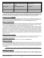


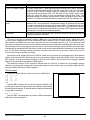
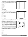


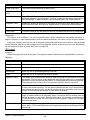

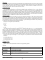

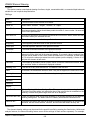
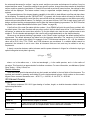

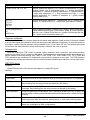

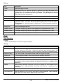
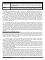
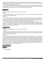


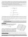


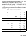
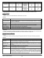
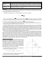


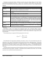


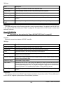
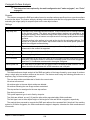


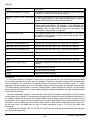


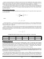
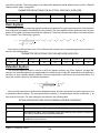
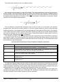


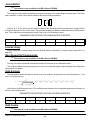


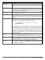
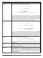


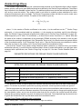

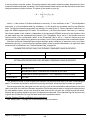
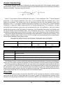

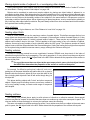


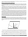

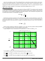


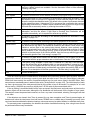
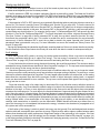


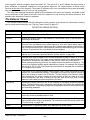
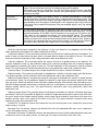


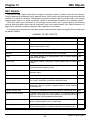


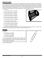

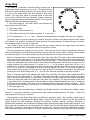
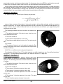

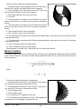


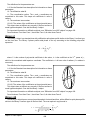

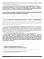

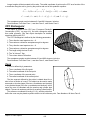
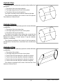
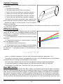


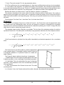


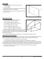


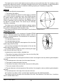
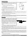
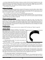
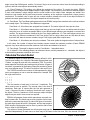

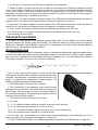


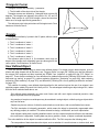


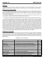


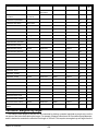


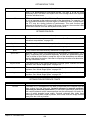


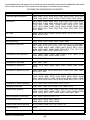


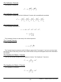
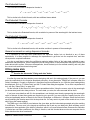


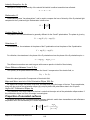

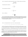


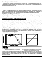
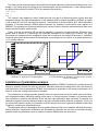


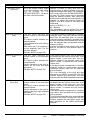
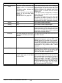


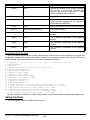
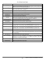


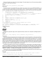

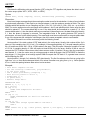

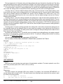

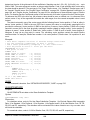


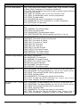

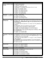

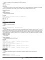
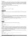


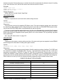

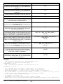

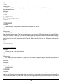
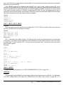


![Guida di SYNC™ HD - akmedia.[bleep]digidesign.](http://vs1.manualzilla.com/store/data/006124188_1-822f431325888ec14269d9216e9ac6fc-150x150.png)