Download AN INTERACTIVE HISTORY AND GEOGRAPHY OF MEXICO

AN INTERACTIVE HISTORY AND GEOGRAPHY OF MEXICO USING
MAP OBJECTS FOR JAVA
_______________
A Thesis
Presented to the
Faculty of
San Diego State University
_______________
In Partial Fulfillment
of the Requirements for the Degree
Master of Science
in
Computer Science
_______________
by
Paola Alvarez-Alzas
Summer 2012
iii
Copyright © 2012
by
Paola Alvarez-Alzas
All Rights Reserved
iv
DEDICATION
I would like to dedicate this thesis work to my family. Especially my parents for their
love, endless support and encouragement in everything that I have ever decided to take on
and for being always there for me, in the good and the bad times.
v
ABSTRACT OF THE THESIS
An Interactive History and Geography of Mexico Using Map
Objects for Java
by
Paola Alvarez-Alzas
Master of Science in Computer Science
San Diego State University, 2012
Mexico is a country rich in history, culture, traditions and biodiversity, among other
things. The motivation for this thesis project comes from the desire to show the user of this
application some of this country’s richness.
The multimedia application developed as part of this work will cover a general
overview of Mexico’s Pre-Hispanic period when Mesoamerica (a region and culture area in
the Americas that extended from Central Mexico to Belize, Guatemala, El Salvador,
Honduras, Nicaragua and Costa Rica) developed and flourished (2000 BC – 1519 AD). This
period included the Olmec, Mayan, Aztec civilizations, among many others, that rose and fell
leaving behind an incredible amount of contributions to today’s Mathematics, Physics,
Astronomy, Arts, etc.
The application will provide a couple of interactive maps of Mexico showing the
areas covered by the Mesoamerican cultures and relevant information about each of them. It
will also provide maps showing the location of the main mountain peaks, ranges and bodies
of water in the Mexico of today.
vi
TABLE OF CONTENTS
PAGE
ABSTRACT ...............................................................................................................................v
LIST OF TABLES ................................................................................................................... ix
LIST OF FIGURES ...................................................................................................................x
ACKNOWLEDGEMENTS ................................................................................................... xiii
CHAPTER
1
INTRODUCTION .........................................................................................................1 2
TECHNOLOGIES USED ..............................................................................................3 2.1 Java SE (Standard Edition) ................................................................................3 2.2 MapObjects Java Edition (MOJO23).................................................................4 2.3 Web Technologies (HTML, CSS, JavaScript) ...................................................4 2.4 NetBeans (IDE) ..................................................................................................5 3
SOFTWARE REQUIREMENTS ..................................................................................6 3.1 Architectural Requirements ...............................................................................7 3.2 Functional Requirements ...................................................................................7 3.3 Non-Functional Requirements ...........................................................................7 3.4 Usability .............................................................................................................7 4
DATA COLLECTION AND ANALYSIS ..................................................................13 5
SOFTWARE IMPLEMENTATION ...........................................................................17 5.1 Localization......................................................................................................17 5.2 Start Page .........................................................................................................19 5.3 Application’s Main Window............................................................................19 5.4 Creation of the Map Layers .............................................................................19 5.4.1 Point Layers ............................................................................................19 5.4.2 Polyline and Polygon Layers ..................................................................22 5.4.3 Creation of a Layer from a Selection ......................................................25 5.5 Application’s Toolbars.....................................................................................27 5.5.1 Zoom/Pan Toolbar ..................................................................................27 vii
5.5.1.1 Previous Extent ..............................................................................28 5.5.1.2 Next Extent ....................................................................................28 5.5.1.3 Zoom to Active Layer ....................................................................28 5.5.1.4 Zoom to Full Extent .......................................................................28 5.5.1.5 Zoom In ..........................................................................................29 5.5.1.6 Zoom Out .......................................................................................29 5.5.1.7 Pan..................................................................................................29 5.5.1.8 Pan in One Direction ......................................................................29 5.5.1.9 Identify ...........................................................................................30 5.5.2 Selection Toolbar ....................................................................................30 5.5.2.1 Find ................................................................................................32 5.5.2.2 Query Builder.................................................................................32 5.5.2.3 Select Features ...............................................................................32 5.5.2.4 Clear All Selection .........................................................................32 5.5.2.5 Buffer .............................................................................................35 5.5.2.6 Attributes........................................................................................35 5.5.3 Customized Toolbar ................................................................................35 5.5.3.1 Print ................................................................................................35 5.5.3.2 Add Layer ......................................................................................35 5.5.3.3 Remove Layer ................................................................................37 5.5.3.4 Legend Editor.................................................................................37 5.5.3.5 Cursor (Arrow)...............................................................................37 5.5.3.6 Hotlink ...........................................................................................37 5.5.3.7 Select Language Tool ....................................................................41 5.5.3.8 Help Tool .......................................................................................41 5.5.3.9 Create Point Layer .........................................................................41 5.5.3.10 Create Polyline Layer ..................................................................41 5.5.3.11 Create Layer from Selection ........................................................44 5.6 Application’s Menus ........................................................................................44 5.6.1 File ..........................................................................................................44 5.6.2 Physiography...........................................................................................44 5.6.3 Mesoamerica Periods ..............................................................................47 viii
5.6.4 Mesoamerican Civilizations....................................................................47 5.6.5 Quizzes and Games .................................................................................47 5.6.6 Help .........................................................................................................52 6
CONCLUSIONS AND OBSTACLES ........................................................................67 7
FUTURE WORK .........................................................................................................69 REFERENCES ........................................................................................................................71 ix
LIST OF TABLES
PAGE
Table 3.1. Architectural Requirement: Platform Independence ................................................7 Table 3.2. Functional Requirement: Mexico’s Mountain Peaks................................................8 Table 3.3. Functional Requirement: Mexico’s Mountain Ranges .............................................8 Table 3.4. Functional Requirement: Mexico’s Rivers ...............................................................8 Table 3.5. Functional Requirement: Mexico’s Lakes ................................................................9 Table 3.6. Functional Requirement: Mesoamerica Timeline.....................................................9 Table 3.7. Functional Requirement: Mesoamerican Sites .........................................................9 Table 3.8. Functional Requirement: Mesoamerica Region .....................................................10 Table 3.9. Functional Requirement: Mesoamerican Civilizations...........................................10 Table 3.10. Functional Requirement: Quizzes and Games ......................................................10 Table 3.11. Non-Functional Requirement: Localization .........................................................11 Table 3.12. Usability Requirement: Information Display .......................................................11 Table 3.13. Usability Requirement: ZoomPan Toolbar ...........................................................11 Table 3.14. Usability Requirement: SelectionToolbar ............................................................12 Table 3.15. Usability Requirement: Help Tools ......................................................................12 Table 3.16. Usability Requirement: Modify Map’s Appearance .............................................12 x
LIST OF FIGURES
PAGE
Figure 4.1. Highest mountain peaks CSV file .........................................................................14 Figure 4.2. Mesoamerica’s pre-Hispanic borders. ...................................................................16 Figure 5.1. Select Language dialog..........................................................................................17 Figure 5.2. Localization property file. .....................................................................................18 Figure 5.3. Application’s start page. ........................................................................................20 Figure 5.4. Application’s main window. .................................................................................21 Figure 5.5. Code snippet to process CSV files for point layers. ..............................................22 Figure 5.6. Mexico’s highest mountain peaks map. ................................................................23 Figure 5.7. Code snippet to track a series of coordinates, based on the mouse’s pointer
movement. ....................................................................................................................24 Figure 5.8. Code snippet to process CSV files for polyline layers. .........................................25 Figure 5.9. Prehispanic Mesoamerica Region map .................................................................26 Figure 5.10. Code snippet to create the lakes layer from a selection of data...........................27 Figure 5.11. Zoom/pan toolbar. ...............................................................................................28 Figure 5.12. Previous extent tool button. .................................................................................28 Figure 5.13. Next extent tool button. .......................................................................................28 Figure 5.14. Zoom to active layer tool button. ........................................................................28 Figure 5.15. Zoom to full extent tool button. ...........................................................................29 Figure 5.16. Zoom in tool button. ............................................................................................29 Figure 5.17. Zoom out tool button. ..........................................................................................29 Figure 5.18. Pan tool button. ....................................................................................................29 Figure 5.19. Pan in one direction tool button...........................................................................30 Figure 5.20. Pan in one direction’s drop down list. .................................................................30 Figure 5.21. Identify tool button. .............................................................................................30 Figure 5.22. Identify tool’s table..............................................................................................31 Figure 5.23. Selection toolbar. .................................................................................................31 Figure 5.24. Find tool button. ..................................................................................................32 Figure 5.25. Find tool’s dialog. ................................................................................................33 xi
Figure 5.26. Query builder tool button. ...................................................................................33 Figure 5.27. Query builder tool’s dialog. .................................................................................34 Figure 5.28. Select features tool button. ..................................................................................35 Figure 5.29. Select features’ drop down list. ...........................................................................35 Figure 5.30. Select features tool used to draw a rectangle.......................................................36 Figure 5.31. Clear all selection tool button. .............................................................................37 Figure 5.32. Buffer tool button. ...............................................................................................37 Figure 5.33. Buffer tool’s dialog..............................................................................................38 Figure 5.34. Attributes tool button. ..........................................................................................39 Figure 5.35. Attributes table. ...................................................................................................40 Figure 5.36. Customized toolbar. .............................................................................................41 Figure 5.37. Print tool button. ..................................................................................................41 Figure 5.38. Add layer tool button. ..........................................................................................41 Figure 5.39. Add layer dialog. .................................................................................................42 Figure 5.40. Map of the highest mountain peaks after adding the main rivers layer...............43 Figure 5.41. Remove layer tool button. ...................................................................................44 Figure 5.42. Legend editor tool button. ...................................................................................44 Figure 5.43. Legend editor’s dialog tab to format features......................................................45 Figure 5.44. Legend editor’s dialog tab to format labels. ........................................................46 Figure 5.45. Cursor (arrow) tool button. ..................................................................................47 Figure 5.46. Hotlink tool button. .............................................................................................47 Figure 5.47. Hotlink tool used on the highest mountain peak’s map. .....................................48 Figure 5.48. Hotlink tool used on the main Mayan site’s map. ...............................................49 Figure 5.49. Archeological site’s web page. ............................................................................50 Figure 5.50. Audio icon. ..........................................................................................................51 Figure 5.51. Code snippet to integrate the hotlink tool to the application. ..............................51 Figure 5.52. Code snippet from the hotlink’s pick adapter class. ............................................51 Figure 5.53. Select language tool button. ................................................................................51 Figure 5.54. Help tool button. ..................................................................................................52 Figure 5.55. Help tip window. .................................................................................................53 Figure 5.56. Create point layer tool button. .............................................................................54 Figure 5.57. Create polyline layer tool button. ........................................................................54 xii
Figure 5.58. Create layer from selection tool button. ..............................................................54 Figure 5.59. File menu. ............................................................................................................54 Figure 5.60. Physiography menu. ............................................................................................54 Figure 5.61. Main mountain ranges in Mexico map. ...............................................................55 Figure 5.62. Main rivers in Mexico map. ................................................................................56 Figure 5.63. Main lakes in Mexico map. .................................................................................57 Figure 5.64. Mesoamerica periods menu. ................................................................................58 Figure 5.65. Main post-classic sites in Mesoamerica. .............................................................59 Figure 5.66. Mesoamerica’s sites timeline. .............................................................................60 Figure 5.67. Mesoamerican civilizations menu. ......................................................................61 Figure 5.68. Main sites founded by the Mayan Civilization....................................................62 Figure 5.69.Civilizations timeline (1200 BC)..........................................................................63 Figure 5.70. Quizzes and games menu. ...................................................................................63 Figure 5.71. Mesoamerica’s quiz. ............................................................................................64 Figure 5.72. Game on Mayan glyphs. ......................................................................................65 Figure 5.73. Help menu. ..........................................................................................................65 Figure 5.74. Quick start guide for the application. ..................................................................66 xiii
ACKNOWLEDGEMENTS
I would like to thank Dr. Carl Eckberg for agreeing to be my advisor and for his
suggestion to take on this project. His support, knowledge, patience and encouragement were
crucial for the completion of this work.
I would like to thank Professor Maricruz Alzás and Dr. Paula De Vos for their
valuable input during the conversations we had that ultimately produced the main
requirements for the application developed as part of this work.
Finally, I would also like to thank Professor Michael E. O’Sullivan and Dr. Joseph
Lewis for agreeing to be part of my Thesis Committee and for taking the time to read this
work.
1
CHAPTER 1
INTRODUCTION
The purpose of this thesis work is to provide an interactive bilingual learning tool of
Mexico’s Pre-Hispanic history and physiography for English and Spanish speaking high
school and college students. Due to the younger generation’s exposure to a great deal of
technology, students in today’s world crave a change in the learning processes that are
available to them. These processes should include multimedia material and a greater
interaction with technology that facilitates and enriches their learning experiences. The aim
of this work is to contribute to that learning experience and make it more enjoyable and
fulfilling.
Some of the key features the application, developed as part of this project, provides
are: the ability to switch between languages (English and Spanish) at any time, not only when
the application first runs. Another feature that supports the bilingual part of this tool is the
inclusion of sound files that will help, especially the non-native Spanish speakers, pronounce
the name of the presented map features (like the Mesoamerican archeological sites). Most of
the maps included, as part of this application, use several icon images that facilitate to the
user the location of a certain feature on the map. Two dynamic timelines are also made
available in this tool to make it easier for the user to better understand and assimilate the
events in the key time periods of Mesoamerica’s history.
This application was developed as a Geographical Information System (GIS) in order
to present to the user different types of geographical data in the form of interactive maps.
This allows the possibility to create dynamic searches, based on user queries, to spatial data.
This thesis document contains 7 chapters. In these, all the steps followed in the
development process of this application are discussed in detail, from the collection of the
software requirements, the data gathering, and the implementation to the conclusions and
future work.
2
In the second chapter of this document, “Technologies Used”, all the technologies
used in the implementation of the tool will be listed and briefly described, highlighting the
main reason why they were chosen.
The third chapter, “Software Requirements”, will go over the methodology followed
for the collection of the requirements for this project. It will list, describe and classify all of
them.
The fourth chapter, “Data Collection and Analysis”, will cover the tools and methods
used for the collection and preparation of the data used to create all the map layers presented
in this application.
The fifth chapter, “Software Implementation”, talks about how each part of this tool
was implemented. It contains several screen shots and some code snippets that will guide the
reader in the understanding of this process.
The last two chapters of this document, “Conclusions and Obstacles” and “Future
Work”, will include lessons learned during this process, the multiple obstacles or difficulties
found in the implementation stage and possible future enhancements to the developed
application as well as areas of research.
3
CHAPTER 2
TECHNOLOGIES USED
For the development of this project some of the core technologies used were:

Programming language: Java Platform, Standard Edition. Java SE 7u2 (1.7.0_02
version) [1].

Application Programming Interface: MapObjects Java Edition (MOJO23).

Web Technologies: HyperText Markup Language (HTML), Cascade Style Sheets
(CSS) and JavaScript.

Integrated Development Environment (IDE): NetBeans.
In the next few sections each technology will be briefly described along with the reasons why
it was chosen.
2.1 JAVA SE (STANDARD EDITION)
Java is a programming language that derives much of its syntax from C and C++ but
has a simpler object model [2]. Java applications are typically compiled to bytecode (class
file) that can run on any Java Virtual Machine (JVM) regardless of computer architecture.
This means that code that runs on one platform does not need to be recompiled to run on
another [2]. This platform independence feature makes this language ideal for the
development of this project.
Java is licensed under the GNU General Public License therefore making it free/open
source software and a very cost-effective option.
Another advantage of using this language for the development of this project, is how
easy is to deploy Java applications. Java uses the Java Archive (JAR) file format which
enables you to bundle multiple files in a single archive file that contains all the class files
(compiled code) and all the auxiliary resources associated with your application [3]. This
JAR file format also allows you to digitally sign the contents for security, especially when
downloading from the internet. Most importantly, it eliminates the need to use a windows
installer, which keeps your application portable.
4
2.2 MAPOBJECTS JAVA EDITION (MOJO23)
This API for Java is a product of ESRI (Environmental Systems Research Institute),
headquartered in Redlands, California [4].
The version used for this project was 2.3. This package version contains several
libraries developed in Java that a programmer can use to create and customize Java
applications in the area of Geographic Information Science (GIS) which covers systems
designed to capture, store, manipulate, analyze, manage, and present all types of
geographical data [5].
Some of the core functionality that this API provides the programmer with is the
possibility of displaying and manipulating maps (based on geographical data) and the ability
to perform queries on its spatial information [4].
MapObjects also lets you merge easily two java-based Graphical User Interface
(GUI) frameworks, AWT (Abstract Windowing Toolkit) and Swing. The use of these two
powerful frameworks allows the developer to customize, to the developer’s needs, the GUI
elements provided by the MapObjects API and create new ones.
The fact that the MapObjects library was written in Java makes it the perfect
companion to the programming language chosen for this project.
2.3 WEB TECHNOLOGIES (HTML, CSS, JAVASCRIPT)
HTML is the main markup language for displaying web pages and other information
that can be displayed in a web browser. CSS is a style sheet language that defines the
appearance and layout of text and other material that is part of documents written in HTML
[6].
JavaScript is a prototype-based scripting language that is dynamic, weakly typed and
has first-class functions. It is primarily used in the form of client-side script language in order
to create enhanced user interfaces and dynamic websites [7].
These three languages were used in the creation of the web pages that are an
important part of this user application.
HTML, CSS and JavaScript are open standards and interpreted, to a certain degree, in
most of today’s web browsers.
5
2.4 NETBEANS (IDE)
This tool was chosen as the Integrated Development Environment to create this
application because it provides a simple to use but yet powerful editor for the Java Platform.
It is available for free, and it is included with the Java SE download on Oracle’s web page
[8].
6
CHAPTER 3
SOFTWARE REQUIREMENTS
Agile development was the process in which the development of this application, in a
much smaller scale, was based on. It is defined as an iterative and incremental (evolutionary)
approach to software development which is performed in a highly collaborative manner by
self-organizing teams within an effective governance framework with “just enough”
ceremony that produces high quality solutions in a cost effective and timely manner which
meets the changing needs of its stakeholders [9].
One of the methodologies suggested by the Agile process is Extreme Programming
(XP). This was the method adopted for this project. Extreme Programming is a method that
stresses customer satisfaction. Instead of delivering everything you could possibly want on
some date far in the future this process delivers the software you need as you need it.
Extreme Programming empowers developers to confidently respond to changing customer
requirements, even late in the life cycle [10]. This methodology promotes frequent releases
or prototypes in short development cycles, constant code review and unit testing of all the
code.
One of the techniques suggested, in Extreme Programming, for the recollection of the
requirements for an application is the creation of User Stories. These stories are written by
the customers as things that the system needs to do for them. They are similar to usage
scenarios, except that they are not limited to describing a user interface. They are in the
format of about three sentences of text written by the customer in their terminology without
techno-syntax [11]. User stories also drive the creation of acceptance tests or criteria to verify
that a certain feature has been correctly implemented.
Developers estimate how long the stories might take to implement. Each story will
get a 1, 2 or 3 week estimate in "ideal development time" [11].
The gathering of user stories for the development of this project was based on
interviews and conversations with Dr. Paula De Vos, professor of Mexican History at San
Diego State University, Maricruz Alzás Almagro professor of Mexican History and
7
Geography at Colegio Cadi, Tijuana B.C., and Dr. Carl Eckberg, professor of Computer
Science at SDSU and my advisor for this thesis.
The format in which the collected user stories are presented below is loosely based in
the template found here [12].
The user stories are also presented in different groups. This grouping was based in the
classification given in the Software Requirements Specification defined by the IEEE Std 8301998 [13].
3.1 ARCHITECTURAL REQUIREMENTS
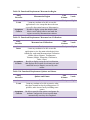
For the architectural requirements of this project see Table 3.1.
Table 3.1. Architectural Requirement: Platform Independence
Story
Narrative
As a
I want
Acceptance
Criteria
Platform Independence
User
I want to be able to use this application in any
computer
All the users of this application (students and
teachers) will be able to use it no matter the
system they have access to
Time
Estimate
1 week
Priority
High
3.2 FUNCTIONAL REQUIREMENTS
For the functional requirements of this project see Table 3.2, Table 3.3, Table 3.4,
Table 3.5, Table 3.6, Table 3.7, Table 3.8., Table 3.9, and Table 3.10.
3.3 NON-FUNCTIONAL REQUIREMENTS
For the non-functional requirements of this project see Table 3.11.
3.4 USABILITY
For the usability requirements of this project see Table 3.12, Table 3.13, Table 3.14,
Table 3.15, and Table 3.16.
8
Table 3.2. Functional Requirement: Mexico’s Mountain Peaks
Story
Narrative
As a
I want
Acceptance
Criteria
Mexico’s Mountain Peaks
Teacher
I want my students to be able to use this
application to view the main mountain peaks
in Mexico’s map.
Be able to locate the main Mexico’s peaks on
a map and be able to view information about
them.
Time
Estimate
Priority
2 week
High
Table 3.3. Functional Requirement: Mexico’s Mountain Ranges
Story
Narrative
As a
I want
Acceptance
Criteria
Mexico’s Mountain Ranges
Teacher
I want my students to be able to use this
application to view the main mountain ranges
in Mexico’s map
Be able to locate the main Mexico’s
mountain ranges on a map and be able to
view information about them
Time
Estimate
3 week
Priority
High
Time
Estimate
2 week
Priority
High
Table 3.4. Functional Requirement: Mexico’s Rivers
Story
Narrative
As a
I want
Acceptance
Criteria
Mexico’s Rivers
Teacher
I want my students to be able to use this
application to view the main rivers in
Mexico’s map.
Be able to locate the main Mexico’s rivers
on a map and be able to view information
about them
9
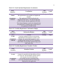
Table 3.5. Functional Requirement: Mexico’s Lakes
Story
Narrative
As a
I want
Acceptance
Criteria
Mexico’s Lakes
Teacher
I want my students to be able to use this
application to view the main lakes in
Mexico’s map
Be able to locate the main Mexico’s lakes on
a map and be able to view information about
them
Time
Estimate
2 week
Priority
High
Time
Estimate
2 week
Priority
High
Time
Estimate
3 week
Priority
High
Table 3.6. Functional Requirement: Mesoamerica Timeline
Story
Narrative
Mesoamerica Timeline
As a
I want
Teacher
I want my students to be able to view a
timeline of Mesoamerica’s main civilizations
Acceptance
Criteria
Be able to display a timeline that includes
information about all the archeological sites
founded during Mesoamerica’s apogee
Table 3.7. Functional Requirement: Mesoamerican Sites
Story
Narrative
As a
I want
Acceptance
Criteria
Mesoamerican Sites
Teacher
I want my students to be able to use this
application to view the location of archeological
sites founded over Mesoamerica’s different
periods: Pre-Classic, Classic and Post-Classic
Be able to locate Mesoamerica’s most important
archeological sites on a map of Mexico-Central
America given a specific period of time
10
Table 3.8. Functional Requirement: Mesoamerica Region
Story
Narrative
As a
I want
Acceptance
Criteria
Mesoamerica Region
Time
Estimate
2 week
Priority
High
Time
Estimate
3 week
Priority
High
Time
Estimate
2 week
Priority
High
Teacher
I want my students to be able to use this
application to view a map that shows the area
covered by the region known as Mesoamerica
Be able to display a map that includes both
Mexico and Central America and mark the
region covered by Mesoamerican cultures
Table 3.9. Functional Requirement: Mesoamerican Civilizations
Story
Narrative
As a
I want
Acceptance
Criteria
Mesoamerican Civilizations
Teacher
I want my students to be able to use this
application to view the main archeological sites
founded by each main Mesoamerican civilization
(Olmec, Maya, Zapotec, Teotihuacana,
Totonaca, Mixtec, Purepecha, Chichimeca,
Toltec, Aztec)
Be able to display a map for each civilization
that displays the location of each main site and
marks the area (or Empire) covered by each
culture
Table 3.10. Functional Requirement: Quizzes and Games
Story
Narrative
As a
I want
Acceptance
Criteria
Quizzes and Games
Teacher
I want my students to be able to practice what
they have learned in class by taking quizzes. If
possible, make it more fun by including some
games
Be able to provide some quizzes and games for
students. And provide a way to grade them
automatically once they are completed
11
Table 3.11. Non-Functional Requirement: Localization
Story
Narrative
As a
I want
Acceptance
Criteria
Localization
User
The application to be available in English and
Spanish.
This application will be localized in the
languages listed above. The desired language
will be selected when the application first runs.
The selected language can also be changed when
the application is running using a menu item or
the appropriate toolbar button.
Time
Estimate
2 week
Priority
High
Time
Estimate
3 week
Priority
High
Time
Estimate
2 week
Priority
High
Table 3.12. Usability Requirement: Information Display
Story
Narrative
As a
I want
Acceptance
Criteria
Information Display
Teacher
I want my students to have access to more
information on the material covered in class
Display the required information in a userfriendly manner using Java GUI components
and HTML web pages that include images and
some audio files
Table 3.13. Usability Requirement: ZoomPan Toolbar
Story
Narrative
As a
I want
Acceptance
Criteria
ZoomPan Toolbar
User
I want to be provided with the ability to Zoom
in, Zoom out, Pan and Identify all the features
that are part of each map displayed
Successfully be able to perform all the
previously listed functions on all the maps
displayed by the application
12
Table 3.14. Usability Requirement: SelectionToolbar
Story
Narrative
As a
I want
Acceptance
Criteria
Selection Toolbar
User
I want to be provided with the ability to ask
the system for the location of a specific feature
Provide the user with tools to query the system
on certain spatial information, select and
highlight specific features on a map.
Time
Estimate
2 week
Priority
High
Time
Estimate
2 week
Priority
High
Time
Estimate
2 week
Priority
High
Table 3.15. Usability Requirement: Help Tools
Story
Narrative
As a
I want
Acceptance
Criteria
Help Tools
User
I want to have access to some sort of manual in
order to figure out how to use the application
Provide the user of the application with a User
Manual and a help tool, easily accessible from
the menu bar. The help tool will provide a way
to find out how to use the toolbar buttons
Table 3.16. Usability Requirement: Modify Map’s Appearance
Story
Narrative
As a
I want
Acceptance
Criteria
Modify Map’s Appearance
User
I want to be provided with the ability to modify
the appearance of the displayed maps (colors,
labels, etc)
Provide the user with an appearance editor
where the color of the map, features and legends
can be updated. Also provide the user with
menu options to add or delete layers from a
map.
13
CHAPTER 4
DATA COLLECTION AND ANALYSIS
For the implementation of this project a great amount of data was required. The
sources for all the data collected for the implementation of this application are listed and
briefly discussed in the next few sections.
A three step process was generally followed in the creation of all the map layers.

Collection of geographical coordinates for the physical features of all the maps
presented.

CSV (Comma-Separated Values) files were generated using the previous collected
coordinates. CSV files store tabular data (numbers and data) in plain text format.
They consist of any number of records, separated by line breaks of some kind; each
record consists of fields, separated by some character or string, most commonly a
literal comma or tab [14]. See Figure 4.1.
Similar CSV files, like the one presented in Figure 4.1 were prepared for all the map
layers presented as part of this application.

Implementation of Java code to read the CSV files and generate the appropriate type
of layer (point, polyline or polygon) in SHP format (shapefile) in order to be
displayed using the Map Objects API. The shapefile format is a geospatial vector data
format for GIS software that was developed by ESRI, it is currently an open
specification [15].
For the following point layers all the GPS (Global Positioning System) coordinates
were obtained through two different tools:

WikiProject Geographical Coordinates [16], a tool that is used by cartographers
around the world to obtain latitude and longitude coordinates of a particular physical
world feature [17].

GeoHack, a modified version of map sources from Egil Kvaleberg's GIS extension.
This tool functions as a web service that provides links to various mapping services,
given specific geographical coordinates, in order to locate them with different
applications like Google Earth, Google Maps, Nokia Maps, MapQuest, etc. [18].
These are the point layers that were constructed using the two previously mentioned
tools:
14
Figure 4.1. Highest mountain peaks CSV file. The first and second fields are the
longitude and latitude respectively. The third and fourth are the name of the peak and
the states in Mexico it’s in and the last field is the elevation of the peak in ft (for the
Spanish version of the application this value was converted to meters).

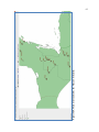
Mexico’s Highest Mountain Peaks: The 30 highest mountain peaks were obtained
from the list of highest peaks in Mexico found in this non-commercial database [19].
For this point layer a map of the states of Mexico was used as a base layer.

Mesoamerica’s Pre-Classic, Classic and Post-Classic Sites: The main sites for each
period in Mesoamerica’s history were obtained through research in texts
recommended by Dr. De Vos and Professor Alzás [20-26]. For this point layer a map
of the Mexico-Central America region was used as a base layer.

Mesoamerican civilization’s sites (Olmec, Mayan, Aztec, Zapotec, Teotihuacana,
Mixtec, Toltec, Totonaca, Chichimeca, Purépecha): The main sites for each
Mesoamerican civilization were obtained through research in texts recommended by
Dr. De Vos and Professor Alzás [20-26]. For this point layers a map of the MexicoCentral America region was used as a base layer.
The polyline and polygon layers listed below were created using different sources.

Mexico’s states: The data used to create the states layer was obtained from the
ArcGIS application, a Geographical Information System (GIS) developed by ESRI
[27] that provides, as part of its sample data, information on the states of Mexico with
15
coastlines, international boundaries, and state boundaries. This layer was used as a
base for other map layers presented in this application.

Mexico-Central America borders: The data used to create this layer was obtained
from the U.S. Geological Survey website. This website provides a world vector
shoreline of the Mexico and Central America region [28]. This layer was used as a
base for other map layers presented in this application.

Mexico’s Main Mountain Ranges: The data obtained to create this layer was
obtained from Peakbagger, a non-commercial web site that supports a large dynamic
database of peaks, ranges and climbers [19].
This large mountain ranges database is based on a hierarchical classification that
divides the entire land surface of the earth into ranges and sub ranges. The full
classification’s rules can be found here [29].
The data for the mountain ranges’ borders presented on this website using Google
Maps’ web service, was used to draw the six main mountain ranges (Sierra Madre
Occidental, Sierra Madre Oriental, Mexican Plateau, Cordillera Neovolcánica, West
Coast Ranges and Sierra Madre del Sur) on a map of Mexico.
For this layer a map of the states of Mexico was used as a base layer.

Mexico’s Main Rivers: The data used to create the rivers layer was obtained from
the ArcGIS application, a Geographical Information System (GIS) developed by
ESRI [27] that provides, as part of its sample data, information on the location of the
rivers on Mexico’s map.
For this layer a map of the states of Mexico was used as a base layer.

Mexico’s Main Lakes: The data used to create the lakes layer was obtained from
DIVA-GIS, a website that provides free geographic data from any country in the
world. The development of DIVA-GIS has been supported by global organizations
like Biodiversity International and the University of California Berkeley, among
others [30].
The data obtained from [30] to create the lakes layer, contained some unnecessary
information, for this particular project. It included data about some water areas that
referred to artificial lakes, dams or they were just no relevant to the Geography
Program of Studies described by professor Alzás. For this reason, an algorithm
needed to be implemented to extract the desired data and create the appropriate layer
from this selection. The process followed to achieve this will be discussed in the
Implementation chapter of this document. For this layer a map of the states of Mexico
was used as a base layer.

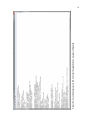
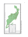
Mesoamerica’s Region: Since no accurate GIS data is available for the Pre-Hispanic
Mesoamerica’s borders, the Mesoamerica Region layer was created as an
approximation of what that area used to cover considering the location of the
archeological sites founded by the ten major cultures that developed in the region.
Data from the Foundation for the Advancement of Mesoamerican Studies, Inc
16
(FAMSI) [31] and visual maps provided here [22-26] were used for the creation of
this layer. See Figure 4.2 [32].
For this layer a map of the Mexico-Central America region was used as a base layer.

Mesoamerica’s civilizations borders (Olmec, Maya, Zapotec, Aztec, Teotihuacana,
Mixtec, Toltec, Totonaca, Chichimeca, Purépecha): Since not very accurate GIS
data is available for Pre-Hispanic Mesoamerica’s civilizations borders, each culture’s
area layer was created as an approximation of what it used to cover considering the
location of the archeological sites founded by a given civilization. Data from the
Foundation for the Advancement of Mesoamerican Studies, Inc (FAMSI) [31] and
visual maps provided here [22-26] were used for the creation of these layers.
For these layers a map of the Mexico-Central America region was used as a base layer.
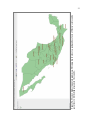
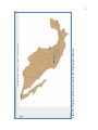
Figure 4.2. Mesoamerica’s pre-Hispanic borders. The borders of the 3 most important
civilizations (Olmec, Mayan, Aztec) are also seen in this figure. Source: A. LAUDUN, The
Maya astronaut: Pakal the great. Wordpress, http://alaudun77.wordpress.com/author/
alaudun/, accessed June 2012, 2011.
17
CHAPTER 5
SOFTWARE IMPLEMENTATION
In this chapter the process followed for the implementation of this application will be
discussed. Several screen shots will be presented to provide a visual guide to the reader.
5.1 LOCALIZATION
The localization of this application was introduced as early as possible in the
implementation process.
When the user first runs the application, a dialog (see Figure 5.1) will be displayed.
This way the user will select the language of preference. From this point on, all the messages
displayed by the program will be localized in the previously selected language.
Figure 5.1. Select Language dialog.
The localization for this application was implemented using the java library
ResourceBundle. Two property files (files that contain each localized message as a pair of
strings, key-value, per line), one with the localized messages in English and the other one
with the messages in Spanish (see Figure 5.2) were created to work with this library.
Figure 5.2. Localization property file. Contains the application’s messages in Spanish.
18
19
5.2 START PAGE
After the user selects the language of preference, the “Start Page” for the application
is displayed. The purpose of this page is to provide the user with a home page were he/she
will have access to a “Quick Start Guide” on how to use the program, and where a list of all
the main menus will be shown (see Figure 5.3).
5.3 APPLICATION’S MAIN WINDOW
The application’s main window is divided in several parts indicated in Figure 5.4.
Most of the parts indicated in Figure 5.4 are very intuitive, and further explained in
the user manual. In this document I’m just going to add a little more information on the
“Table of Contents” and the “Status Bar”.
The “Table of Contents” is located to the left of the map area and it contains a list of
all the map’s layers currently displayed, it also serves as the legend’s definition that identifies
each feature on the map. The “Status Bar” displays the coordinate in the map to which the
cursor currently points at, and it is dynamically updated as the mouse’s pointer moves.
5.4 CREATION OF THE MAP LAYERS
In order to present to the user of this application all the maps the way they are, two or
more layers needed to be created for each map and rendered in a user-friendly way.
5.4.1 Point Layers
For the creation of the point layers, the method described in the chapter “Data
Collection and Analysis” was followed. Part of the code used to parse the CSV files, like the
one presented in Figure 4.1., can be seen in Figure 5.5.
The code snippet seen in Figure 5.5 was modified depending on the point layer that
was being created, in order to process the appropriate data for it. In this case, the CSV file
being processed was the one for the Highest Mountain Peaks in Mexico, so the data to be
parsed was the GPS coordinate (longitude, latitude), the peak’s name, the states where the
peak is in, the mountain range to which it belongs and the peak’s elevation.
Figure 5.3. Application’s start page.
20
Figure 5.4 Application’s main window.
21
22
java.io.File inputFile = fileChooser.getSelectedFile();
java.io.FileReader fileReader = new java.io.FileReader(inputFile);
java.io.BufferedReader bufferedReader = new java.io.BufferedReader(fileReader);
String inputString;
double longitude, latitude;
int pointIndex=0;
while((inputString = bufferedReader.readLine())!= null){
java.util.StringTokenizer st = new java.util.StringTokenizer(inputString,",");
longitude = Double.parseDouble(st.nextToken());
latitude = Double.parseDouble(st.nextToken());
peakNames.add(st.nextToken());
states.add(st.nextToken());
ranges.add(st.nextToken());
elevations.add(st.nextToken());
basePointsArray.insertPoint(pointIndex++, new com.esri.mo2.cs.geom.Point(longitude,latitude));
}
Figure 5.5 Code snippet to process CSV files for point layers.
After the data was parsed from each CSV file, the appropriate database fields were
created and its type defined using the Map Objects API (this code is not presented as part of
this document). With the data parsed and the database fields defined, the Feature Layer was
created and the display properties rendered (color, graphics, etc) in the way they are
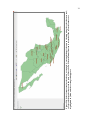
presented in the application. The point layer(s) was then added to the appropriate base layer.
In the case of the Highest Mountain Peaks layer, the base layer was the states of Mexico, as
seen in Figure 5.6.
5.4.2 Polyline and Polygon Layers
For the creation of the polyline and polygon layers, the method described in the
chapter “Data Collection and Analysis" was followed.
The creation of these types of layers was more complex than the creation of point
layers, especially when accurate GIS data was not available, like it was the case for the PreHispanic Mesoamerica’s borders, the Mesoamerican Civilizations borders and the Mountain
Ranges.
For the previous reason, code needed to be implemented to be able to draw on a map,
register the GPS coordinates and save them to a CSV file to be parsed later into a polyline
layer. A snippet of the code used for this can be seen in Figure 5.7.
Once the CSV file for the polyline layer was generated, the file was parsed. A snippet
of the code used to parse the CSV files for polyline layers can be seen in Figure 5.8.
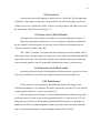
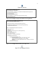
Figure 5.6. Mexico’s highest mountain peaks map. This map has two layers, a polygon base layer of Mexico’s states and a
point layer with the highest peaks in the country.
23
24
currentMap.addMouseMotionListener(new MouseMotionAdapter() {
@Override
public void mouseMoved(MouseEvent mouseEvent)
{
com.esri.mo2.cs.geom.Point worldPoint = null;
if(currentMap.getLayerCount() > 0)
//The Map is not empty
{
worldPoint = currentMap.transformPixelToWorld(mouseEvent.getX(), mouseEvent.getY());
String coordinate = "X:" + statusBarDecimalFormat.format(worldPoint.getX()) + " " +
"Y:" + statusBarDecimalFormat.format(worldPoint.getY());
statusBar.setText(coordinate);
String coordinate2 = statusBarDecimalFormat.format(worldPoint.getX()) + "," +
statusBarDecimalFormat.format(worldPoint.getY());
try {
// Create file
FileWriter fstream = new FileWriter("out.csv",true);
BufferedWriter out = new BufferedWriter(fstream);
out.write("," + coordinate2);
//Close the output stream
out.close();
}
catch (Exception e) {
System.err.println("Error: " + e.getMessage());
}
} //End if
else { statusBar.setText("X:0.000 Y:0.000"); }
} } );
//End of addMouseMotionListener
Figure 5.7. Code snippet to track a series of coordinates, based on the mouse’s pointer
movement.
The code snippet seen in Figure 5.8 was modified depending on the polyline layer
that was being created, in order to process the appropriate data for it. In the CSV file
processed with the previous code each line has all the GPS coordinates for each polyline that
is part of the layer being created.
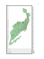
After the data was parsed from each CSV file, the appropriate database fields were
created and its type defined using the Map Objects API (this code is not presented as part of
this document). With the data parsed and the database fields defined, the Polyline Feature
Layer was created and the display properties rendered (color, graphics, etc) in the way they
are presented in this application. The polyline layer(s) was then added to the appropriate base
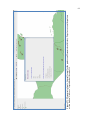
layer. In the case of the Mesoamerica’s Region map, the base layer was the Mexico-Central
America layer, as seen in Figure 5.9.
25
java.io.File inputFile = fileChooser.getSelectedFile();
java.io.FileReader fileReader = new java.io.FileReader(inputFile);
java.io.BufferedReader bufferedReader = new java.io.BufferedReader(fileReader);
String inputString;
com.esri.mo2.cs.geom.BasePointsArray bpa = new com.esri.mo2.cs.geom.BasePointsArray();
double longitude, latitude;
int pointIndex=0;
while((inputString = bufferedReader.readLine())!= null)
{
java.util.StringTokenizer st = new java.util.StringTokenizer(s,",");
int limit = st.countTokens();
for(int index=0; index<limit/2; index++)
{
longitude = Double.parseDouble(st.nextToken());
latitude = Double.parseDouble(st.nextToken());
bpa.insertPoint(pointIndex++, new com.esri.mo2.cs.geom.Point(longitude,latitude));
}
//polylinesNames.add(st.nextToken());
//Uncommented when there's text or data fields in CSV file
//highestPoints.add(st.nextToken());
//areas.add(st.nextToken());
//extents.add(st.nextToken());
polylines.add(new com.esri.mo2.cs.geom.BasePolyline(new com.esri.mo2.cs.geom.BasePath(bpa)));
bpa = new com.esri.mo2.cs.geom.BasePointsArray();
pointIndex=0;
}
Figure 5.8 Code snippet to process CSV files for polyline layers.
A similar process to the one described for the creation of polyline layers can be
followed for the creation of polygon layers by using the appropriate Map Object API classes.
5.4.3 Creation of a Layer from a Selection
For the creation of Mexico’s main lakes layer a special algorithm needed to be
implemented to select the desired data because of the reasons explained in the “Data
Collection and Analysis” chapter.
A snippet of the code used for this purpose can be seen in Figure 5.10.
The way the code, seen in Figure 5.10, works is by using the source data from the
lakes layer obtained from [30] and querying its database using a form of SQL (Structured
Query Language) supported by the Map Objects API. The SQL query was constructed based
on input from professor Alzás, who provided the name of the lakes that she wanted to see in
the final Mexico’s lakes map.
With the obtained data, from querying the lake’s database, the Mexico’s main lakes
layer was generated in shapefile format.
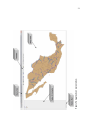
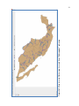
Figure 5.9. Prehispanic Mesoamerica Region map
26
27
com.esri.mo2.map.dpy.FeatureLayer featureLayer =
(com.esri.mo2.map.dpy.FeatureLayer)currentMap.getLayer("Lakes");
com.esri.mo2.file.shp.DbaseTable tableData = new com.esri.mo2.file.shp.DbaseTable(
new
java.io.File("C:\\ESRI\\MOJ23\\Samples\\Data\\MEXICO\\Lakes.dbf"));
com.esri.mo2.data.feat.BaseQueryFilter queryFilter = new com.esri.mo2.data.feat.BaseQueryFilter();
queryFilter.setWhereClause("NAME like '%MIRAMAR%' or NAME like '%BACALAR%' or NAME like
'%CATEMACO%'
or NAME like '%CHAPALA%' " +
"or NAME like '%CUITZEO%' or NAME like '%YURIRIA%' or NAME like
'%PATZCUARO%'
or NAME like '%SAYULA%' " +
"or NAME like '%TEQUESQUITENGO%' or NAME like '%TEXCOCO%'
or NAME like '%GUZMAN%' " +
"or NAME like '%ZIRAHUEN%' or NAME like '%TRES PALOS%' or
(NAME like 'LAGUNA SALADA' and HYC_DESCRI like 'NonPerennial/Intermittent/Fluctuating') " +
"or NAME like '%TAMIAHUA%'");
queryFilter.setSubFields(featureLayer.getFeatureClass().getFields());
com.esri.mo2.map.dpy.FeatureLayer newLayer =
featureLayer.createSelectionLayer(featureLayer.select(queryFilter));
com.esri.mo2.file.shp.ShapefileWriter.writeFeatureLayer(newLayer,MEXICO_DATA_DIRECTORY_PATH,"Sel
ection",2);
Figure 5.10 Code snippet to create the lakes layer from a selection of data.
5.5 APPLICATION’S TOOLBARS
This application has three main toolbars. The Zoom/Pan Toolbar and the Selection
Toolbar are the two standard ones that should be present, in some form, in most GIS
applications that provide the user with an interactive map. These two toolbars are supported
by the Map Objects API and can be customized, in some way, for a particular GIS
application. The third toolbar was specifically created and customized for this project. In the
next few sections the previously mentioned toolbars will be briefly discussed. The
customized toolbar will be reviewed in more depth.
5.5.1 Zoom/Pan Toolbar
The Zoom/Pan Toolbar contains nine standard buttons. The functionality of every one
of them is briefly described in this section.
The toolbar seen in Figure 5.11 provides the user with the ability to manipulate the
current map by zooming on it and moving it in a specific direction. It also allows to identify
each feature on the current map.
28
Figure 5.11. Zoom/pan toolbar.
5.5.1.1 PREVIOUS EXTENT
Every time before the user modifies the scale of the map by using any of the zoom or
pan tools, a view of the map with its current scale gets saved to the extent history. So when
this tool button is used (see Figure 5.12), it zooms the map to the previous extent stored in
the extent history (it works like an undo for maps).
Figure 5.12. Previous extent tool button.
5.5.1.2 NEXT EXTENT
Every time before the user modifies the scale of the map by using any of the zoom or
pan tools, a view of the map with its current scale gets saved to the extent history. So when
this tool button is used (see Figure 5.13), it zooms to the next extent stored in the extent
history (it works like a redo for maps).
Figure 5.13. Next extent tool button.
5.5.1.3 ZOOM TO ACTIVE LAYER
This tool zooms the map to the extent of all the features that are part of the selected
layer(s). This way the view of the map, after this button is pressed (see Figure 5.14), it’s
scaled in a way that includes all the selected layer’s features and not more.
Figure 5.14. Zoom to active layer tool button.
5.5.1.4 ZOOM TO FULL EXTENT
This tool zooms the map to the extent of all layers within the map. This means that
after pressing this tool button (see Figure 5.15) we get an eagle eye view of the entire map
changing the scale of it appropriately.
29
Figure 5.15. Zoom to full extent tool button.
5.5.1.5 ZOOM IN
Provides a tool for clicking or dragging a rectangle on the map in order to zoom in.
The scale for the current map is modified accordingly. When using this tool (see Figure
5.16), the cursor changes to a “zoom in magnifier” to indicate that the tool is active. In order
to unselect the tool, the cursor tool button needs to be pressed (see section 5.5.3.5).
Figure 5.16. Zoom in tool button.
5.5.1.6 ZOOM OUT
Provides a tool for clicking or dragging a rectangle on the map in order to zoom out.
The scale for the current map is modified accordingly. When using this tool (see Figure
5.17), the cursor changes to a “zoom out magnifier” to indicate that the tool is active. In order
to unselect the tool, the cursor tool button needs to be pressed (see section 5.5.3.5).
Figure 5.17. Zoom out tool button.
5.5.1.7 PAN
This button provides a tool for dragging the map to a new location without altering
the map’s scale. When using this tool (see Figure 5.18), the cursor changes to a hand shape to
indicate that the tool is active. In order to unselect the tool, the arrow (cursor) tool button
needs to be pressed (see section 5.5.3.5).
Figure 5.18. Pan tool button.
5.5.1.8 PAN IN ONE DIRECTION
Pans the map in one of four directions: north, south, east, or west. When pressing this
tool button (see Figure 5.19), the drop down list, seen in Figure 5.20, is displayed.
30
Figure 5.19. Pan in one direction tool button.
Figure 5.20. Pan in one direction’s drop down list.
The list includes the options for panning the map north, south, east or west. The
percentage to pan is based on the current map’s extent and it is applied toward the clicked
panbar direction. This percentage can be programmatically modified through the public
method setPanPace(double percentage) of the PanPanel class.
5.5.1.9 IDENTIFY
Performs and identify function on the features that are part of the currently selected
layer. When using this tool (see Figure 5.21), the cursor changes to a smaller pointer that has
an information sign on top, to indicate that the tool is active. In order to unselect the tool, the
arrow (cursor) tool button needs to be pressed (see section 5.5.3.5).
Figure 5.21. Identify tool button.
In the case of the highest mountain peaks in Mexico map, if you use the “Identify”
tool button and select the peak “Sierra La Madera,” by clicking on it, this feature will be
highlighted and after that, a table displaying all the peak’s properties will be displayed to the
user. This table can be seen in Figure 5.22.
5.5.2 Selection Toolbar
The Selection Toolbar contains seven standard buttons. The functionality of six of
them will be briefly described in this section.
The Selection toolbar, seen in Figure 5.23, provides the user with the ability to query
on spatial data associated with the current map.
Figure 5.23. Selection toolbar.
Figure 5.22. Identify tool’s table. Table displayed when using identify tool on a map’s feature.
31
32
5.5.2.1 FIND
This tool (see Figure 5.24) opens a dialog to locate features on the current map whose
attributes contain an end-user provided string. It doesn’t have to be an exact match. As long
as the provided string is contained in any database field of any feature that is part of the
selected layer, it will return the first match and the feature will be highlighted on the map.
Figure 5.25 illustrates the “Find” dialog.
Figure 5.24. Find tool button.
5.5.2.2 QUERY BUILDER
This tool (see Figure 5.26) opens a dialog for locating features based on a query that
an end-user constructs using a subset of SQL logical and comparison operators provided in
the same dialog. After the statement gets executed the result records are displayed in a table
and the result features are highlighted on the map. Figure 5.27 shows what the “Query
Builder” dialog looks like.
5.5.2.3 SELECT FEATURES
This tool (see Figure 5.28) provides a way for selecting features by rubberbanding a
shape on the map. When the user presses the tool button, the drop down list seen in Figure
5.29 is displayed.
The list (seen in Figure 5.29) includes the options for using a rectangle, circle, line or
polygon shape to draw on the map in order to select the desired features. When the user
releases the left-click mouse button the features within the drawn shape are automatically
selected and highlighted in yellow. See Figure 5.30.
5.5.2.4 CLEAR ALL SELECTION
This tool (see Figure 5.31) provides the user with the ability to clear all the selected
features that result from using the previously discussed tools that are part of the Selection
toolbar.
Figure 5.26. Query builder tool button.
Figure 5.25. Find tool’s dialog. Dialog displayed when using the find tool with the input string: “Sierra La Madera.” Notice
how the feature found is highlighted on the map.
33
Figure 5.27. Query builder tool’s dialog. Dialog displayed when using the query builder tool with the SQL statement
(StateName like ‘%Nuevo León%’) which returns all the peaks located in the Mexican state of Nuevo León. Notice how all the
peaks found in this state are highlighted in yellow.
34
35
Figure 5.28. Select features tool button.
Figure 5.29. Select features’ drop down list.
5.5.2.5 BUFFER
Pressing this toolbar button (see Figure 5.32) opens a dialog for constructing a buffer
polygon around the currently selected features. This dialog can be seen in Figure 5.33.
5.5.2.6 ATTRIBUTES
This tool (see Figure 5.34) displays the attributes of the currently selected features.
All the database records of the current layer are displayed in the table but only the records of
the selected features are highlighted in blue. See Figure 5.35.
5.5.3 Customized Toolbar
The Customized Toolbar contains eleven buttons (see Figure 5.36). Their
functionality is briefly described in this section.
5.5.3.1 PRINT
This tool (see Figure 5.37) provides the user with the usual printing functionality
found in most user applications. It calls the native print dialog used in the operating system.
It prints the current map on display.
5.5.3.2 ADD LAYER
This tool (see Figure 5.38) opens a dialog to be able to browse for the map layer (in
SHP format) that wants to be added to the map currently displayed. See Figure 5.39.
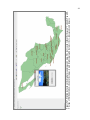
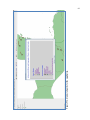
After browsing and selecting the desired layer to be added to the map, the new layer
is added, the map is refreshed and the legend for the new layer appears on top of the Table of
Contents area, located to the left of the map. See Figure 5.40.
Figure 5.30. Select features tool used to draw a rectangle. A rectangle shape is drawn on the map using the select features tool,
to select all the peaks that are in the state of Nuevo León. When the mouse button is released all the selected features are
highlighted in yellow and the rectangle disappears.
36
37
Figure 5.31. Clear all selection tool button.
Figure 5.32. Buffer tool button.
5.5.3.3 REMOVE LAYER
In order to use this tool (see Figure 5.41), the layer to be removed should be selected.
To select a layer is necessary to click its legend on the table of contents area. After the layer
is selected, pressing the Remove Layer button will automatically remove the layer, update
the map and the table of contents.
5.5.3.4 LEGEND EDITOR
This tool (see Figure 5.42) allows the user to modify the appearance of each layer that
is part of the map currently displayed. The layer to be modified needs to be selected first. The
legend editor provides the user with the option of modifying the layer’s color and labels
through a dialog with different tabs. See Figure 5.43 and 5.44.
5.5.3.5 CURSOR (ARROW)
This tool (see Figure 5.45) provides a way for the user to unselect a map tool (that
changes the shape of the cursor like Zoom In, Zoom Out, Pan, Identify, Hotlink and Help
Tool) by changing the cursor back to the normal pointer.
5.5.3.6 HOTLINK
This button (see Figure 5.46) provides the user with a tool (the cursor changes to a
lightning bolt) to identify the features on the selected layer by clicking on them and
displaying either a purely java constructed window containing further information about the
feature or by displaying a picture of the feature and providing a web page link that contains
other interesting information. The two types of hotlink windows created for this application
can be seen in Figure 5.47 and Figure 5.48.
Figure 5.33. Buffer tool’s dialog. The buffer dialog provides a way to input the buffer distance based on the currently selected
features. It also allows to decide if the features within the buffer zone need to be selected and therefore highlighted in yellow.
38
39
Figure 5.34. Attributes tool button.
The Hotlink window seen in Figure 5.48 contains, at the bottom, a “Site Information”
button. When pressed, this button will open a browser window with the appropriate web page
created for the site. All the web pages created for this application have the format seen in
Figure 5.49.
In order to unselect this tool, the arrow (cursor) tool button needs to be pressed (see
section 5.5.3.5).
For both versions of this application (English and Spanish), audio files with the
correct pronunciation of the archeological site’s name where added to the site’s web page to
help especially non-Spanish speakers. To be able to listen to the audio file, the user has to
click on the audio icon (see Figure 5.50). Javascript needs to be enabled on the web browser
in order to use this feature. The web browser will display a message to let the user know
about this. These audio files are also played every time the user clicks with the hotlink tool
on a map’s feature, before either one of the two types of hotlink windows are displayed.
To generate the audio files in MP3 format, the Google translate tool [33] was used.
This tool generates audio files based on an input query string. To force the Spanish
pronunciation in the audio, Spanish characters, like the accent (á), were sometimes used to
define the strong syllable and avoid an Anglicized pronunciation of the name.
The code snippet, seen in Figure 5.51, gives an idea on how the hotlink tool was
integrated and implemented in this project.
In the code snippet (see Figure 5.51), based on the code found in the GISMexico
Class, it can be seen that the Hotlink tool extends the functionality provided by the
previously discussed Identify tool. A pick listener was added to the Hotlink tool in order to
identify when a map feature is clicked on and display the appropriate information window.
In the code snippet, seen in Figure 5.52, part of the implementation for the
PickAdapter class is presented. The method foundData identifies which layer the pick event
occurred on and calls the appropriate method to display the information for the feature where
the hotlink tool was used on.
Figure 5.35. Attributes table. The record of the selected feature on the map, in this case “Picacho San Onofre” (seen in yellow
on the map), is highlighted in blue in the displayed attributes table for the mountain peaks layer.
40
41
Figure 5.36. Customized toolbar.
Figure 5.37. Print tool button.
Figure 5.38. Add layer tool button.
5.5.3.7 SELECT LANGUAGE TOOL
With this tool (see Figure 5.53) the user will be able to switch between the English
and Spanish version of the program, once the application is already running.
5.5.3.8 HELP TOOL
With this tool (see Figure 5.54), the user will be able to right-click on a tool button
and see a help window pop up with information on how that tool works. See Figure 5.55.
When using this tool the cursor will change its shape into a pointer with a question
mark to the side. To unselect the Help Tool, and go back to the normal cursor shape, the
Cursor tool button needs to be pressed (see section 5.5.3.5).
5.5.3.9 CREATE POINT LAYER
This button (see Figure 5.56) was the GUI (Graphical User Interface) used to run the
code implemented for the creation of point layers described in section 5.4.1 This button
opens a dialog to browse for the appropriate CSV file.
This functionality was only enabled on the development stage in order to create all
the point layers for this application. It will not be enabled for the end users of this program
because it requires a little more understanding of how GIS data is generated.
5.5.3.10 CREATE POLYLINE LAYER
This button (see Figure 5.57) was the GUI (Graphical User Interface) used to run the
code implemented for the creation of polyline layers described in section 5.4.2. This button
opens a dialog to browse for the appropriate CSV file.
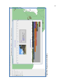
Figure 5.39. Add layer dialog. This dialog allows the user to select the new layer to be added to the current map. The Mexican
Rivers layer is the layer about to be added, in this case.
42
Figure 5.40. Map of the highest mountain peaks after adding the main rivers layer. The map and the table of contents are
updated.
43
44
Figure 5.41. Remove layer tool button.
Figure 5.42. Legend editor tool button.
This functionality was only enabled on the development stage for the same reasons
described above.
5.5.3.11 CREATE LAYER FROM SELECTION
This button (see Figure 5.58) was the GUI (Graphical User Interface) used to run the
code implemented for the creation of layers from a selection of GIS Data, this process was
described in section 5.4.3. This button automatically creates a layer from a selection of the
data that its part of the current layer, based on a provided SQL query.
This functionality was only enabled on the development stage for the same reasons
described in sections 5.5.3.9 and 5.5.3.10.
5.6 APPLICATION’S MENUS
This application has six main menus. In the next few sections these menus will be
briefly discussed.
5.6.1 File
The File menu (see Figure 5.59) provides access to basic functions that can be
performed on the current map: Add Layer, Remove Layer, Legend Editor, Language
Options, Print and Exit. These menu items (except for “Exit” that has no button on the
toolbar) provide the same functionality than that provided by the tool buttons of the same
name described in section 5.5.3. Having these functions as menu items gives the user another
way of accessing the same functionality.
5.6.2 Physiography
The Physiograhy menu (see Figure 5.60) provides the user with access to Mexico’s
Hydrographic and Topographic Maps. In the Topographic sub-menu, the maps for the main
Figure 5.43. Legend editor’s dialog tab to format features. The selected layer is the rivers layer (a polyline layer), so the type,
the color and the thickness of the line can be modified.
45
Figure 5.44. Legend editor’s dialog tab to format labels. The formatting includes the label’s position from the feature’s
perspective.
46
47
Figure 5.45. Cursor (arrow) tool button.
Figure 5.46. Hotlink tool button.
mountain peaks (see Figure 5.6) and the main mountain ranges (see Figure 5.61) in Mexico
can be seen. In the Hydrographic sub-menu the maps for the main rivers (see Figure 5.62)
and the main lakes (see Figure 5.63) in Mexico can be accessed.
5.6.3 Mesoamerica Periods
This menu (see Figure 5.64) provides the user with access to different Mesoamerica’s
maps that illustrate the main archeological sites in the region depending on the period. For
each period (Pre-Classic, Classic, Post-Classic) there’s a corresponding menu item. See
Figure 5.65.
There’s also the menu item, “Mesoamerica Timeline”, that provides the user with an
interactive timeline based on the main archeological sites founded during Mesoamerica’s
history. See Figure 5.66.
5.6.4 Mesoamerican Civilizations
This menu (see Figure 5.67) provides the user with access to different Mesoamerica’s
Civilizations maps that illustrate the area that each one used to cover as well as the main sites
that were founded by each group (see Figure 5.68). This menu also provides access to a map
that shows the region covered by Mesoamerica’s cultures (see Figure 5.9). A dynamic
timeline is also available, the map layers change as the user interacts with it (see Figure
5.69).
5.6.5 Quizzes and Games
This menu (see Figure 5.70) provides the user with access to a couple of quizzes and
games about Mesoamerica’s history. The purpose of this menu is to provide the students with
a way to assimilate all the lessons learned in a more fun way.
Figure 5.47. Hotlink tool used on the highest mountain peak’s map. The tool is used to identify the peak “Volcán de Tequila”.
The type of Hotlink window, shown in the image, is used for physiographic features (rivers, lakes, peaks and ranges).
48
Figure 5.48. Hotlink tool used on the main Mayan site’s map. The tool is used to identify the ancient site of “Uxmal”. The type
of hotlink window, shown in the image, is used for archeological features. Notice the button “Site Information”.
49
Figure 5.49. Archeological site’s web page. Web page displayed when clicking on the “Site Information” button seen in Figure
5.48. Notice the audio icon (see Figure 5.50) to the right of the archeological site’s name.
50
51
Figure 5.50. Audio icon.
//Code snippet from GISMexico Main Class
private Identify hotlink = new Identify();
GISMexicoPickAdapter pickListener = new GISMexicoPickAdapter(selectedLanguage, this);
hotlink.addPickListener(pickListener);
hotlink.setPickWidth(40);
hotlink.setSelectedLayer(activeLayer);
JButton hotlinkButton = new JButton(new ImageIcon(HOTLINK_ICON));
gisToolBar.add(hotlinkButton);
Figure 5.51. Code snippet to integrate the hotlink tool to the application.
//Code snippet from the GISMexicoPickAdapter Class
public void foundData(PickEvent pickEvent)
{
FeatureLayer featureLayer =(FeatureLayer)pickEvent.getLayer();
…
else if(featureLayer.getName().equals(messages.getString("MayaSites")))
displayMayaSitesInfo(pickEvent);
…
}
public void displayMayaSitesInfo(PickEvent pickEvent)
{
Feature feature = null;
Fields fields;
com.esri.mo2.data.feat.Cursor cursor = pickEvent.getCursor();
if(cursor != null)
feature = (Feature)cursor.next();
fields = feature.getFields();
String siteName = (String)feature.getValue(2);
…
else if(siteName.equals("Uxmal"))
{
HotlinkWindow hotlinkWindow = new
HotlinkWindow(GISMexico.HTML_DATA_DIRECTORY_PATH +
messages.getString("UxmalFilename")+ ".html", siteName,
GISMexico.HTML_IMAGES_DIRECTORY_PATH + "Uxmal.jpg", ownerFrame,
messages);
hotlinkWindow.setVisible(true);
}
}
Figure 5.52. Code snippet from the hotlink’s pick adapter class.
Figure 5.53. Select language tool button.
52
Figure 5.54. Help tool button.
The quizzes will get graded after the student completes them and the correct answers
in comparison with the given answers, will be highlighted. Depending on the game, the
questions will be graded on a per “question” basis. See Figure 5.71 and 5.72.
5.6.6 Help
This menu (see Figure 5.73) provides the user with access to a “Quick Start Guide”
on how to use this application. It also provides some information about the developer, the
version of the program and a copyright notice. See Figure 5.74.
Figure 5.55. Help tip window. Window displayed when the help tool is used on the hotlink button.
53
54
Figure 5.56. Create point layer tool button.
Figure 5.57. Create polyline layer tool button.
Figure 5.58. Create layer from selection tool button.
Figure 5.59. File menu.
Figure 5.60. Physiography menu.
Figure 5.61. Main mountain ranges in Mexico map. Accessed from “Topography” sub-menu.
55
Figure 5.62. Main rivers in Mexico map. Accessed from “Hydrography” sub-menu.
56
Figure 5.63. Main lakes in Mexico map. Accessed from “Hydrography” sub-menu.
57
58
Figure 5.64. Mesoamerica periods menu.
Figure 5.65. Main post-classic sites in Mesoamerica. Maps for the main pre-classic and classic sites are also accessed from the
“Mesoamerica Periods” menu.
59
Figure 5.66. Mesoamerica’s sites timeline.
60
61
Figure 5.67. Mesoamerican civilizations menu.
Figure 5.68. Main sites founded by the Mayan Civilization.
62
Figure 5.70. Quizzes and games menu.
Figure 5.69.Civilizations timeline (1200 BC).
63
Figure 5.71. Mesoamerica’s quiz. General format for the quizzes on Mesoamerica’s history. To get a score on the quiz an
action button “Get Score” is provided at the end of it.
64
Figure 5.73. Help menu.
Figure 5.72. Game on Mayan glyphs. The student has to guess what the Mayan glyph means.
65
Figure 5.74. Quick start guide for the application.
66
67
CHAPTER 6
CONCLUSIONS AND OBSTACLES
This thesis work was extremely motivating for me, not only because one of the goals
was showcasing Mexico’s history, geography and culture but because the ultimate goal of
this work was to provide the students of Mexico’s history and geography, with an interactive
tool that supports and enhances their learning process in today’s world. I strongly believe that
technology is going to be a central part (it already is in a lot of ways) of the education of the
future, so to have been able to develop this tool is very fulfilling.
There were a lot of obstacles and difficulties to overcome during the development of
this tool, mainly because I have not had a lot of experience with the two main technologies
(Java and MapObjects) used for this project. For this same reason, I thought that the
development time for some of the features was going to be shorter that it actually ended up
being. But that is expected when dealing with technologies that you are not very familiar
with.
The creation of some of the layers, especially the mountain ranges layer, proved a
little more challenging than I expected. The GIS data was hard to find and drawing and
rendering the ranges’ borders took a lot of time and research within the MapObjects API.
Another difficulty that I encountered often was that some of the features and methods
supported by the MapObjects API were buggy and it was hard to get around this. Even
simple things like the location of feature’s labels proved really frustrating when dealing with
polygons, especially if these were considerably small (like in the case of the lakes map). The
polygons would sometimes get lost underneath the labels. One would think that this is a
small fix, and in theory it should be, but the methods and constants provided by the
MapObjects API to do this, would not work at all. In my research for a solution, I found a lot
of comments on this in the ESRI forum by many other developers with similar issues to
mine.
The resizing of the maps was another frequent issue I had, especially because I
applied different zooms to different layers and because I had two different base layers (the
68
Mexico’s states map and the Mexico-Central America region map). Every time I had to
change the zoom on a specific layer I had to update my map’s extent so it would resize
appropriately depending on the map currently displayed. Repainting the map’s labels, when
resizing, was also something that I had to implement. Because of some strange reason, that I
never really figured out, the labels would sometimes disappear from the map when the size of
the main application window was changed, so I had to make sure this never happened by
repainting them every time a resize event occurred.
The learning curve for the Java layout managers, AWT and Swing, was not easy to
take on. I got stuck many times trying to display GUI components in a certain way. Towards
the end of the development it got significantly easier after I gained more understanding on
how they worked.
Like I discussed in the last couple of paragraphs, the technologies used for the
development of this project were sometimes challenging, but I really enjoyed this whole
process because, among other things, it has opened to me the possibility of combining two
things that I truly love: technology and history. To be potentially involved in interactive
knowledge projects like this one, in the near future, paints a really exciting career path for
me.
69
CHAPTER 7
FUTURE WORK
This thesis project leaves a lot of space for future work that could cover really diverse
aspects of Mexico’s history, geography and culture.
Some of the possible areas or features that could be explored or implemented are listed
below:
In the geography area:

Map layers on Mexico’s biogeography that would deal with patterns of species
distribution. It would be especially interesting to create layers that could show
(present and past) geography distribution of animal and plant species.

A Map layer on Mexico’s desert geography.

Map layers on climate trends that could show climate change in Mexico over a
specific period of time.

A map layer on the political divisions in Mexico that includes information on all of
the state’s capitals.
In the historic area:

Continue to further extend the current layers on Mesoamerica’s history and add new
ones. Layers on the tribute network controlled by the Aztec Empire, trade networks
between the different Mesoamerican sites, battles between empires, etc.

Include layers on Mexico’s Colonial History: The Conqueror’s different expeditions,
evangelization areas, battles against the indigenous people, etc.

Mexico’s Independence and Revolution layers: battles against the Spaniards
(Independence), distribution of the different insurgent groups and civil war factions
(Revolution), etc.
In the cultural area:

A map layer on Mexico’s main tourist sites.

A layer on the different cuisine types across the different regions in the country.

Distribution and information on the different indigenous groups.

Information on the distribution of Mexico’s industries, agricultural crops, imports and
exports that support the country’s economy.

A layer with Information on the traditional dances for each region.
70
The amount of quizzes and games presented in this application could also be
increased. In the case of the quizzes, the ability for the teacher to create a quiz could also be
added by implementing the appropriate user interface that allows the input of questions,
multiple options and correct answers. Given the modularity in which the Quiz class was
created, this is easily doable.
The list of features could continue, showing this way that Mexico is a country rich in
history, culture, traditions and biodiversity.
71
REFERENCES
[1]
ORACLE, Java SE 7 update 2. Oracle, http://www.oracle.com/technetwork/java/
javase/7u2-relnotes-1394228.html, accessed January 2012, n.d.
[2]
WIKIPEDIA, Java (programming language). Wikipedia, http://en.wikipedia.org/
wiki/Java_(programming_language), accessed June 2012, 2012.
[3]
ORACLE, Packaging programs in JAR files. Oracle,
http://docs.oracle.com/javase/tutorial/deployment/jar/index.html, accessed June 2012,
n.d.
[4]
C. ECKBERG, Notes on map objects – Java edition. Unpublished notes, 2010.
[5]
WIKIPEDIA, Geographic information system. Wikipedia, http://en.wikipedia.org/wiki/
Geographic_Information_System, accessed June 2012, 2012.
[6]
WIKIPEDIA, HTML. Wikipedia, http://en.wikipedia.org/wiki/Html, accessed June
2012, 2012.
[7]
WIKIPEDIA, JavaScript. Wikipedia, http://en.wikipedia.org/wiki/JavaScript, accessed
June 2012, 2012.
[8]
ORACLE, JDK 7u5 with NetBeans 7.1.2. Oracle, http://www.oracle.com/technetwork/
java/javase/downloads/jdk-7-netbeans-download-432126.html, accessed January
2012, n.d.
[9]
AGILE MODELING, Disciplined agile software development. Agile Modeling,
http://www.agilemodeling.com/essays/agileSoftwareDevelopment.htm, accessed June
2012, n.d.
[10]
D. WELLS, Extreme programming: A gentle introduction. Extreme Programming,
http://www.extremeprogramming.org/, accessed June 2012, 2009.
[11]
D. WELLS, User stories. Extreme Programming,
http://www.extremeprogramming.org/rules/userstories.html, accessed June 2012, n.d.
[12]
C. BROWN, User story template. Better Projects, http://www.betterprojects.net/2011/
03/user-story-template.html, accessed June 2012, 2011.
[13]
IEEE STANDARDS ASSOCIATION, 830-1998 - IEEE recommended practice for
software requirements specifications. IEEE Standards Association,
http://standards.ieee.org/findstds/standard/830-1998.html, accessed June 2012, n.d.
[14]
WIKIPEDIA, Comma-separated values. Wikipedia, http://en.wikipedia.org/wiki/
Comma-separated_values, accessed June 2012, 2012.
[15]
ESRI, ESRI shapefile technical description. ESRI, http://www.esri.com/library/
whitepapers/pdfs/shapefile.pdf, accessed June 2012, 1998.
72
[16]
WIKIMEDIA FOUNDATION, INC., WikiProject geographical coordinates. Wikipedia,
http://en.wikipedia.org/wiki/Wikipedia:WikiProject_Geographical_coordinates,
accessed June 2012, 2012.
[17]
EVOLUTIONZONE, Code and form: Computational aesthetics. Evolutionzone,
http://workshop.evolutionzone.com/2006/10/28/geo-all-geo-coordinates-fromwikipedia/, accessed June 2012, n.d.
[18]
E. KVALEBERG, GeoHack. Wikimedia Toolserver, https://wiki.toolserver.org/view/
GeoHack, accessed June 2012, 2012.
[19]
PEAKBAGGER, Homepage. Peakbagger, http://www.peakbagger.com/, accessed June
2012, n.d.
[20]
M. MEYER, The Course of Mexican History, Oxford University Press, New York,
New York, 2002.
[21]
L. V. FOSTER, A Brief History of Mexico, Facts on File, New York, New York, 1997.
[22]
N. DAVIES, The Ancient Kingdoms of Mexico, Penguin Books, New York, New York,
1991.
[23]
M. D. COE AND R. KOONTZ, Mexico: From the Olmecs to the Aztecs, Thames &
Hudson, New York, New York, 2008.
[24]
WIKIPEDIA, Mesoamerica. Wikipedia, http://en.wikipedia.org/wiki/Mesoamerica,
accessed June 2012, 2012.
[25]
M. LONGHENA, Culturas prehispánicas de México, Guatemala y Honduras, Monclem
Ediciones, México, D. F., 1998.
[26]
R. GOMEZ, L. JAVIER, B. BOSQUED, AND M. CONCEPCION, Culturas Clasicas
Prehispanicas: Las Raices de la America Indigena. Anaya Publishers, Madrid,
Spain,1998.
[27]
ESRI, ArcGIS. ESRI, http://www.esri.com/software/arcgis/index.html, accessed June
2012, n.d.
[28]
U.S. GEOLOGICAL SURVEY, World vector shoreline of the Mexico and Central
America region. U.S. Geological Survey, http://coastalmap.marine.usgs.gov/GISdata/
basemaps/mexico/shoreline/wvs/mexico-cam_wvs_geo_wgs84.htm, accessed June
2012, 2005.
[29]
PEAKBAGGER, Arranging ranges: Mountain ranges of the world. Peakbagger,
http://www.peakbagger.com/RangIndx.aspx, accessed June 2012, n.d.
[30]
DIVA-GIS, Homepage. DIVA-GIS, http://www.diva-gis.org/, accessed June 2012,
2012.
[31]
FOUNDATION FOR THE ADVANCEMENT OF MESOAMERICAN STUDIES, INC., Maps.
Foundation for the Advancement of Mesoamerican Studies, Inc.,
http://www.famsi.org/maps/, accessed June 2012, n.d.
[32]
A. LAUDUN, The Maya astronaut: Pakal the great. Wordpress,
http://alaudun77.wordpress.com/author/alaudun/, accessed June 2012, 2011.
73
[33]
GOOGLE, Google Translate. Google, http://translate.google.com, accessed June 2012,
n.d.