Download fulltext - DiVA Portal

Ultra-low Power Stack-based Processor
for Energy Harvesting Systems
Allan Green
Embedded Computing Systems
Submission date: June 2014
Supervisor:
Snorre Aunet, IET
Norwegian University of Science and Technology
Department of Electronics and Telecommunications
Problem Description
Ultra-low Power Stack Based Processor for Energy Harvesting
Systems
One of the most recent trends in electronics is the Internet of Things. The
transition to these systems is happening. The base for these systems will be
multiple low–energy consuming nodes able to connect different devices
between them. A promising option to replacing the battery on systems is to use
an energy harvesting system.
Energy harvesting systems are battery-less systems powered by energy
sources in the environment, such as heat gradients, light, or vibration. Due to
the limited energy available, these systems often need a small programmable
subsystem for basic control tasks, as well as processing and interpreting
sensor data. This subsystem should be as small as possible to accomplish the
required task while consuming as little as possible of the available energy.
The assignment goal is to implement an ultra-low power stack-based CPU to
be used in an energy harvesting system. The CPU should be integrated in a
complete subsystem with a RAM and low-power peripherals. Basic example
code typical for the application should be written. The stack processor will be
used as a part of a bigger project; therefore it should be designed and
implemented to be compatible with previous and future work. Compatibility will
have a high priority in the project. The architecture should be simulated and
tested. If time allows it, the performance and power consumption of the system
should be compared when implemented with a regular standard cell library, as
well as an ultra-low voltage library.
i
Abstract
The fast evolution of the Internet of Things suggests an unavoidable transition
to this infrastructure in the near future, and to achieve this multiple nodes need
to interconnect and communicate efficiently. All nodes will need a power source
to operate. Most of them will have very low power consumption requirements.
Therefore, a possible solution would be to have an energy harvesting system
for the nodes.
The energy harvesting systems will need a CPU to control all operations and to
manage the power consumption. The goal of this assignment is to create a
base processor capable of controlling the system using ultra-low levels of
power.
The proposed approach for the assignment is to use a stack processor. Using
the J1 processor as a reference, a new architecture was designed. The design
process was done following the design flow tools used by Atmel and covered
the simulation, testing, synthesis and place and route process.
The end result of the assignment was a functional stack processor system with
the capability to communicate with I/O modules using a Wishbone bus. A
custom assembler was created using Arch C to simplify the testing of the
architecture. The design was simulated, synthesized and routed using specific
libraries from Atmel.
The assignment completed a working design flow that will allow the realization
of a proper power analysis in the next phase of development. The stack
processor architecture shows high potential for ultra-low power operations.
Further time and power analysis is needed to have a complete comparison with
other processors.
iii
Preface
This thesis is submitted to the Norwegian University of Science and
Technology in cooperation with Atmel Corporation as a requirement for the
fulfillment of the European Master in Embedded Computer Systems (EMECS)
degree.
This work has been performed at the Atmel office in Trondheim, Norway under
the supervision of Ronan Barzic, and in association with the Department of
Electronics and Telecommunications at NTNU, with Prof. Snorre Aunet as the
university supervisor.
Acknowledgements
I would like to extend my gratitude to my supervisors Ronan Barzic and Prof.
Snore Aunet for their guidance and support through the entire process, to all of
the staff, instructors and my friends in the Erasmus Mundus Embedded
Computing Systems program, and finally to my family and girlfriend for all their
love and unconditional support.
v
vi
Table of Contents
Problem Description ............................................................................................. i
Abstract .............................................................................................................. iii
Preface ............................................................................................................... v
Acknowledgements ......................................................................................... v
Table of Contents.............................................................................................. vii
Table of Figures ................................................................................................. xi
1 Introduction ...................................................................................................... 1
1.1 Internet of Things ...................................................................................... 1
1.2 Motivation: Energy Harvesting .................................................................. 2
1.3 Assignment Interpretation ......................................................................... 3
1.4 Report Organization .................................................................................. 4
2 Background ...................................................................................................... 5
2.1 Stack Processors ...................................................................................... 5
2.1.1 What is a Stack? ................................................................................ 5
2.1.2 Why Use a Stack Processor? ............................................................ 7
2.2 The J1 Processor .................................................................................... 10
2.3 Wishbone Bus ......................................................................................... 12
2.3.1 Wishbone Signals ............................................................................ 12
vii
2.3.2 Wishbone Operation ........................................................................ 14
2.3.2.1 Single Read Cycle .................................................................... 14
2.3.2.2 Single Write Cycle .................................................................... 15
2.4 Design Flow ............................................................................................ 17
2.4.1 Arch C.............................................................................................. 18
3 Implementation .............................................................................................. 21
3.1 Methodology ........................................................................................... 21
3.1.1 Development Basis and Organization ............................................. 21
3.1.2 Choice of Tools................................................................................ 23
3.2 Design Process ....................................................................................... 23
3.2.1 Implementation of the J1 Processor ................................................ 24
3.2.2 Design of the Stack Processor ........................................................ 25
3.2.3 Instruction Set Description ............................................................... 26
3.2.4 Initial Architecture Design ................................................................ 27
3.2.5 The Wishbone Bus .......................................................................... 30
3.2.6 System Integration ........................................................................... 31
3.3 Testing Process ...................................................................................... 33
3.4 Synthesis Process .................................................................................. 35
3.5 Place and Route Process ....................................................................... 38
4 Results ........................................................................................................... 41
viii
4.1 Final Design ............................................................................................ 41
4.2 Simulations ............................................................................................. 42
4.3 Area Distribution and Layout ................................................................... 47
5 Discussion & Future Work.............................................................................. 49
5.1 Power Analysis ....................................................................................... 49
5.2 Stack Merging ......................................................................................... 50
5.3 Wishbone Bus Extension ........................................................................ 51
5.4 Pipeline Optimization .............................................................................. 51
6 References..................................................................................................... 53
7 Appendix ........................................................................................................ 55
7.1 Final RTL Code ....................................................................................... 55
7.1.1 CPU ................................................................................................. 55
7.1.2 Dual Port Ram ................................................................................. 63
7.1.3 Data Stack ....................................................................................... 64
7.1.4 Return Stack .................................................................................... 65
7.1.5 Wishbone Master Module ................................................................ 66
7.1.6 Wishbone Slave Module .................................................................. 67
7.2 ArchC Files ............................................................................................. 70
7.2.1 Stkpc.ac ........................................................................................... 70
7.2.2 Stkpc_isa.ac .................................................................................... 70
ix
7.3 Instruction Set Table ............................................................................... 73
x
Table of Figures
Figure 1-1: The Internet of Thing Evolution [1] ........................................................... 1
Figure 2-1:LIFO PUSH and POP Operations ............................................................. 6
Figure 2-2: Generic Stack Processor Architecture [4] ................................................ 7
Figure 2-3: Add Operation on Stack Processor .......................................................... 8
Figure 2-4: Return Stack Example ............................................................................. 9
Figure 2-5: J1 Architecture Diagram [7].................................................................... 11
Figure 2-6: J1 ALU Instruction Decoding [7]............................................................. 11
Figure 2-7: Master and Slave Wishbone's Interface [8] ............................................ 12
Figure 2-8: Single Read Cycle [8] ............................................................................ 15
Figure 2-9: Single Write Cycle [8] ............................................................................. 16
Figure 2-10: Ideal Design Flow ................................................................................ 17
Figure 3-1: Design Process ...................................................................................... 22
Figure 3-2: Instruction Decoding .............................................................................. 26
Figure 3-3: Initial Architecture Diagram .................................................................... 27
Figure 3-4: Wishbone Bus Connection Diagram ...................................................... 30
Figure 3-5: Stack Processor Hierarchy..................................................................... 32
Figure 3-6: Testing Flow Diagram ............................................................................ 34
Figure 3-7: Synthesis Flow ....................................................................................... 36
xi
Figure 3-8: Different RAM Connections.................................................................... 37
Figure 3-9: Place and Route Flow ............................................................................ 38
Figure 4-1: Final Design Architecture ....................................................................... 41
Figure 4-2: Add Simulation ....................................................................................... 43
Figure 4-3: Call Simulation ....................................................................................... 44
Figure 4-4: Wishbone Bus Communication Example ............................................... 46
Figure 4-5: Area Distribution .................................................................................... 47
Figure 4-6: Place and Route .................................................................................... 48
Figure 5-1: Post-Place and Route Flow.................................................................... 50
Figure 5-2: Stack Merging ........................................................................................ 51
Figure 5-3: Pipeline Modification .............................................................................. 52
xii
1 Introduction
The electronic revolution is a reality. Every day, more gadgets and appliances
are given the capability to interconnect and communicate using the internet. To
better understand the work done in this assignment, insight is needed into the
actual trends and problems internet connected devices face.
1.1 Internet of Things
The internet of things is a fairly new concept, yet it has become rapidly popular
in the last years. Even though an official definition for this term does not exist,
for this assignment it is defined as the attempt to equip all gadgets, objects and
appliances in the world with a way to connect and communicate between them
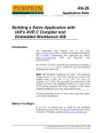
and the internet. To give a bit of perspective, refer to Figure 1-1, provided in a
study by Cisco [1]. The number of connected devices has already surpassed
the world population and bear in mind that 30 years ago, an internet connection
was not commercially available to the general public.
Figure 1-1: The Internet of Thing Evolution [1]
1
1.2 Motivation: Energy Harvesting
The previous figure takes brings the next question: What are the consequences
and problems that emerge when there are so many connected devices in terms
of energy? All the connected devices need an energy source. Some can have
a wired connection and others can be outfitted with a battery. Yet, in many
cases a wired connection is not possible and having a battery brings up the
problem of maintenance.
Changing batteries in some devices can be extremely hard or impossible. An
example of this would be sensors used in the industry. These normally do not
need to be active at all time. Usually, a very short duty cycle is used and
therefore small amounts of energy should be enough to keep them operational.
Energy harvesting is a possible solution for the previously mentioned problem.
Energy harvesting uses ambient energy sources which are free most of the
time; some examples are light, heat differentials, vibrating beams, or
transmitted RF signals. As promising as it may sound, energy harvesting
devices generate only small amounts of energy and they need a system to
control their operation. To get a better insight some examples are shown [2]:

Small solar panels can produce 100s of mW/cm 2 in direct sunlight and
100s of µW/cm2.

Piezoelectric devices using compression or deflection can produce 100s
of µW/cm2 depending on size and construction.

RF energy harvesting collecting antennas can produce 100s of pW/cm2.

Seebeck devices, using temperature gradients, can generate 10s of
µW/cm2 working with body temperatures or 10s of mW/cm2 working with
a furnace exhaust stack temperatures.
Therefore to offer a working solution, the CPU controlling the energy harvesting
needs to work with ultra-low power levels. Otherwise, all of the energy
generated by the system would be used by the CPU controlling the system.
2
The solution proposed is to use a stack processor to achieve an efficient and
ultra-low power consumption system. Stack processors are not new. They were
developed in 1950 and are still being used, mainly due to their simplicity. Yet,
using them to provide a solution to energy harvesting systems is something
that has so far not received any deep research. Previous stack processor
implementations give the advantage of having proper documentation that can
help in the implementation process.
1.3 Assignment Interpretation
Following the assignment description and guidelines given by the tutors, the
following main tasks were identified, all mandatory tasks were completed:
Task 1: (mandatory) Design a stack processor system, including RAM,
communication bus and I/O module.
Task 2: (mandatory) Test and simulate the system.
Task 3: (mandatory) Successfully synthesize the design.
Task 4: (mandatory) Perform place and route of the design.
Task 5: (optional) Perform power analysis.
Task 6: (optional) Load the design to an FPGA board.
Task 7: (optional) Perform energy consumption measurements and
compare the results with other processors.
The above task list was done by both the supervisors and the student after
doing the initial contract; some differences may exist with the initial problem
description, however, these were the final tasks approved by the supervisors.
This assignment will set the foundations for the energy harvesting system;
therefore, proper documentation and implementation of the stack processor are
the highest priority.
It is important to mention that all the work done in the assignment needs to be
compatible with the design flow used at Atmel. Considerable time was needed
to learn and become familiar with the design flow, though this was not part of
the tasks listed for the assignment. The design flow helps the assignment to be
3
reusable and scalable. These two characteristics make the compatibility with
the design flow a priority. Detailed theory and insight on both the Internet of
Things and Energy Harvesting subjects are not within the scope of the
assignment.
1.4 Report Organization
The organization of the report is divided into individual chapters that are briefly
described for the reader’s convenience:

Chapter 1:Introduction gives an overview about the internet of things,
the motivation for this assignment and the assignment tasks and
limitations

Chapter 2: Background describes the basic knowledge needed to fully
understand the assignment report, including: stack processors, the J1
processor, Wishbone communication and the Atmel design flow.

Chapter 3: Implementation covers the methodology, tools and
implementation, starting from each individual element’s point of view up
to the complete unification of the system.

Chapter 4: Results shows the final design and the simulations used to
verify the correct behavior of the system.

Chapter 5: Discussion & Future Work covers final thoughts on the
assignment as well as possible optimizations of the design.
4
2 Background
The goal of this section is to give a brief summary on the basic theory
necessary for accomplishing the present assignment. The first and foremost
point covered is the stack processor, as that is the base for the assignment.
Next, the processor used as a reference, the J1 Processor, is discussed. An
overview of the Wishbone communication protocol and the design flow used at
Atmel are also covered.
2.1 Stack Processors
Stacks have been used for more than over 50 years in the computer
environment. The first proposal for using a stack was made in 1946 in the
computer design of Alan M. Turing as a tool for calling and returning from
subroutines. Later, a formal proposal and a patent was obtained in 1957 by
Klaus Samelson and Friedrich L. Bauer of Germany [3] [4] [5].
It is important to understand that a stack simplified the ability to do recursion
and loops. Their popularity followed a path of ups and downs as history moved
forward. The introduction of Very Large Scale Integration (VLSI) and Complex
Instruction Set Computers (CISC) caused processor design to drift away from
the stack processor, due to the long and comprehensive instructions. However,
with the growth in popularity of Reduced Instruction Set Computers (RISCs)
that proposed a simple instruction set to achieve higher performance, stack
processors became strong candidates for processor designs once again.
2.1.1 What is a Stack?
A stack is one of the simplest ways of storing temporal information. It is an area
of computer memory with a fixed origin but variable size. The data structure
follows the concept of Last-In-First-Out (LIFO). In a LIFO data structure, the
last data that comes into the stack (top of stack) is the first to be removed.
5
Once a memory area is defined for the stack, a stack pointer is needed to point
to the most recently referenced location on the stack. The stack pointer is
normally implemented in the form of a hardware register [4].
One of the advantages of working with a stack is that only two operations can
be used to modify the stack:

Push: Data is introduced to the location pointed by the stack pointer,
also known as the top of stack, and the stack pointer is updated
depending on the size of the data introduced to the stack.

Pop: Data at the current location pointed by the stack pointer is removed
from the stack, and the stack pointer is updated depending on the size of
the data removed to the stack.
It is important that the stack pointer always references the top of stack and is
always updated properly. Failure to do so will lead to loss of information and
faulty execution of the processor.
For this assignment the data introduced or removed from stack will have the
same size as the memory space. Therefore the update of the stack pointers will
always consist of a unitary addition or subtraction.
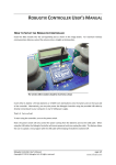
Figure 2-1:LIFO PUSH and POP Operations
6
Figure 2-1 depicts an example of using the push and pop instructions. In this
instance, the value “12” is first pushed onto the stack and then later popped off
of the stack. Notice how the stack pointer (“Top”) is always updated.
2.1.2 Why Use a Stack Processor?
A stack processor design was chosen for the assignment due to certain
benefits it offers. Before explaining the benefits or characteristic in depth, an
overview of a simple stack processor architecture is needed. Figure 2-2 is an
example of generic stack processor architecture from [4].
Figure 2-2: Generic Stack Processor Architecture [4]
The previous figure shows some of the key elements of a stack processor:

Data stack (DS): memory in charge of managing all the operands for the
arithmetic and logic operations.
7

Return stack (RS): memory in charge of storing subroutine return
addresses.

Top of stack (TOS): Last element pushed into the data stack.
The other elements are common to most processors: the program memory,
program counter (PC), memory address register (MA), arithmetic / logic unit
(ALU) and data bus.
Stacks enable benefits in two areas: Basic operand operations and subroutine
calling. An example can explain basic operand operations. A simple addition is
shown in Figure 2-3. The first step pushes the values that need to be added,
the values 12 and 24. Once the values are stored in the data stack, the
operand is sent. The processor takes the two values on the top of the data
stack, adds them, and places the result on the top of the data stack.
Figure 2-3: Add Operation on Stack Processor
What benefits can we see from the previous example? The instructions PUSH
and POP only have one argument. Basic arithmetic and logical operations will
always use the values on the top of the stack. Therefore, the operation
instructions do not require an argument. In a typical RISC processor, a similar
instruction could be done in one instruction but it would need at least three
arguments.
Stack processors have the capability to call subroutines and exit them using the
Return Stack, which follows the same principle as any stack. The only
8
difference is that it stores the subroutine return addresses instead of operands.
Figure 2-4 shows an example in which the return stack is used. Assume the
program counter (PC) increments by one after executing each operation. When
the instruction CALL is executed, the address of the next instruction is stored in
the Return Stack and the PC is updated to the subroutine address. Once the
execution in the subroutine is finished using the EXIT instruction, the
subroutine return address is taken from the Return Stack and is used to update
the PC. Finally the HALT instruction stops the program.
Figure 2-4: Return Stack Example
The previous example shows that with a simple instruction set, stack
processors are able to manage subroutines in a very efficient manner. This
opens the possibility to more complex code structures like loops, conditional
statements, etc. From the previous examples we can summarize some points
about stack processors:

Compact code: Even though operand loads need to be done separately
and the total number of instructions needed for a program is higher than
a normal RISC program, due to the reduced size of the instructions, the
total code size in bytes is less for a stack processor than for a register
file processor.
9

Simple instruction set: the simplicity of the instructions allows a
compiler to be built quickly, making the simulation and testing process
faster and simpler.

Simple return stack: Enables recursion and subroutine execution.

Simple data stacks: Replaces a complex cache system.
Remembering that everything has a downside, the stack processors have also
some disadvantages. The stacks cannot be accessed randomly; therefore
planning ahead is needed to obtain efficient code. Also the instruction set used
by stack processors is not able to reference multiple registers, like RISCs
instruction sets.
2.2 The J1 Processor
The J1 Processor is a very simple 16-Bit stack-based, single cycle processor
created by James Bowman. The J1 is not a general purpose CPU, it was
originally intended for FPGAs and to run the six Ethernet cameras in the Willow
Garage PR2 robot [6].as The J1 uses a very compressed instruction set that
makes it ideal for applications that need a high throughput, such as
uncompressed video streaming. The J1’s simple design, light-weight code and
capability for high throughput make it a great candidate to use as a starting
point for the design of an ultra-low power stack processor.
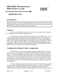
Figure 2-5 shows the basic architecture diagram of the J1, which consists of a
data stack (D), return stack (R), random access memory unit (RAM), decoder
unit and arithmetic unit [7]. The first three are shown twice to simplify graphical
representation.
The J1 was designed for programs written in Forth and implementation of Forth
instructions like duplicate, swap, drop, etc. is simplified. To achieve this, the
instruction decoding uses specific fields as flags for certain events, as Figure
2-6 shows. Specific flags include modifying the data or return stack pointer,
pushing or popping the top of the data or return stack, and more. For further
information please refer to the J1 Paper [7].
10
Figure 2-5: J1 Architecture Diagram [7]
Figure 2-6: J1 ALU Instruction Decoding [7]
11
2.3 Wishbone Bus
The Wishbone bus was selected for this assignment to provide communication
between the stack processor and any external I/O. The following information
was taken from the OpenCores Wishbone User Manual [8].
Figure 2-7: Master and Slave Wishbone's Interface [8]
The Wishbone bus is a popular open source hardware computer bus, which
makes it great to work with due to the many examples and documentation that
exists. The aim of the Wishbone is to allow the connection between different
components inside of a chip, which suits the assignment perfectly.
The
Wishbone is a parallel bus and can work with different bus widths, including 8,
16, 32, and 64 bits, and follows a master slave topology as shown in Figure
2-7. This project will use the 16 bit width due to the fact that the J1 is a 16 bit
processor.
2.3.1 Wishbone Signals
The communication is done based on a clock and multiple signals. The signal
names are standardized and can be divided into three categories: signals
12
common for both slave and master interface, master interface signals and slave
interface signals. Signals can be categorize in 3 types: Signals exclusive to the
master, signals exclusive to the slave and signals that are common for both the
master and the slave. Descriptions of master’s signals and the common signals
follow. Slave signals are omitted due to the similarity they have with the master
signals. For a more complete description of the signals, please refer to the User
Manual [8].
Common Signals for slave and master

CLK_I: Clock input from the system clock, used for synchronizing all
activities done within the wishbone bus.

RST_I: Reset input signal from the system, causes wishbone interface to
restart.

DAT_I(): Data input array used to pass binary data.

DAT_O(): Data output array used to pass binary data.

TGD_I(): Data tag type used to provide more information associated to
DAT_I().

TGD_O(): Data tag type used to provide more information associated to
DAT_O().
Masters Signals

ACK_I: Acknowledgement input; assertion of this signal indicates
termination of bus cycle.

ADR_O(): Address output array; used to pass a binary address.

CYC_O: Cycle bus output; assertion of this signal indicates that a valid
bus cycle is in progress.

STALL_I: Pipeline stall signal indicates current slave cannot accept the
transfer. Only used in pipeline mode.

ERR_I: Error input is used to identify an abnormal cycle termination.

LOCK_O: Lock output; when asserted will make the current bus cycle
uninterruptable.
13

RTY_I: Retry input indicates that interface is not ready to operate and
cycle must be retried.

SEL_O(): Select output array is used to indicate where valid data is
expected on DAT_I().

STB_O: Strobe output indicates a valid data transfer cycle.

TGA_O(): Address tag type; provides extra information associated with
ADR_O().

TGC_O(): Cycle tag type provides extra information associated with bus
cycle.

WE_O(): Write enable output; indicates if current cycle is read or write.
2.3.2 Wishbone Operation
The Wishbone bus has multiple operating modes. The present assignment will
focus on the standard single read cycle (Figure 2-8) and write cycle (Figure
2-9). It is also important to consider that the data sent or received at this time is
the same width as the bus itself (16 Bits). Both read and write will be explained
using the relevant signals for the project [8].
2.3.2.1 Single Read Cycle
The following description is a summary of the information found on the
OpenCores Wishbone manual. It explains how the read cycle works on a
Wishbone interface. The explanation is separated by clock cycles for practical
purposes. Figure 2-8 represents this bus transaction as well.
Clock Edge 0

Master presents valid address on ADR_O.

Master negates WE_O to indicate read cycle.

Master asserts CYC_O to indicate the start of cycle.

Master asserts STB_O to indicate the start of phase.
Clock Edge 1
14

Slave presents valid data on DAT_I().

Slave asserts ACK_I in response to STB_O to indicate valid data.

Master monitors ACK_I and prepares to latch data on DAT_I ().
Clock Edge 2

Master latches data on DAT_I().

Master negates STB_O and CYC_O to indicate end of cycle

Slave negates ACK_I in response to negated STB_O
Figure 2-8: Single Read Cycle [8]
2.3.2.2 Single Write Cycle
The following explains how the write cycle works on a Wishbone interface. The
explanation is once again separated by clock cycles for practical purposes.
Figure 2-9 represents this bus transaction as well.
Clock Edge 0

Master presents valid address on ADR_O.

Master presents valid data on DAT_O.
15

Master asserts WE_O to indicate write cycle.

Master asserts CYC_O to indicate the start of cycle.

Master asserts STB_O to indicate the start of phase.
Clock Edge 1

Slave prepares to latch the data on DAT_O().

Slave asserts ACK_I in response to STB_O to indicate latched data.

Master monitors ACK_I and prepares to terminate the cycle.
Clock Edge 2

Slave latches data on DAT_O().

Master negates STB_O and CYC_O to indicate end of cycle.

Slave negates ACK_I in response to negated STB_O.
Figure 2-9: Single Write Cycle [8]
Both of the previous descriptions assume the slave needs no waiting time to
respond to the master. The actual project implementation has a stall that allows
the slave to have a waiting time, more detail of this will be discussed on
Section 3.2.
16
2.4 Design Flow
Implementation, simulation and testing of a design can become a very time
consuming process. Therefore, a design flow is used to simplify the process.
The goal of the design flow is to use high level language scripts to build all the
tools needed to simulate, test and document the design. The design flow was a
work in progress that took place in parallel to the assignment implementation.
The ideal design is shown in Figure 2-10.
Figure 2-10: Ideal Design Flow
The first step of the design flow represented by section A on Figure 2-10, is to
use docbook documents with xweb termination. These files will have the
description of the architecture and instructions for the processor. These xweb
17
files will be used to generate the documentation PDF and, more importantly,
multiple snippets of Python code. These small pieces of code then will be
united to form the design template.
Ideally, the design template will be the base to generate two sets of files: the
Verilog files for the RTL design and the Arch C files for implementing the
assembler language used by the design, represented by section B on Figure
2-10.
The design flow will also be in charge of installing the compilation tools for
Verilog and Arch C if needed; finally the design flow will do the simulation of the
previously generated Verilog file. The design flow is not the main focus of this
assignment and is still a work in progress. Therefore, changes were applied
continuously during the development of the assignment. The assignment
focused on section B of the design flow, creating the RTL Files and the Arch C
files.
2.4.1 Arch C
A brief introduction taken from the Arch C User Manual [9] will be given to
provide an overall understanding of the process taking place when generating
the stack processor assembler language.
The solution to simplify the development and testing of a design in recent years
has been the use of Architecture Description Languages (ADL). Due to the
increasing complexity of modern designs and time-to-market restraints,
designers are moving from hardware description languages to system level
designs, where
automatic generation of a software toolkit (composed by
assemblers, linkers, compiler and simulators ) is mandatory [10] [11] [9].
Arch C is a language that follows the System C syntax style and is capable of
describing a processor’s architecture and a memory hierarchy. The goal of
Arch C is to provide information at the right abstraction level to provide
18
designers with the tools needed to explore and verify a new architecture
automatically, like assemblers, simulators, linkers and debuggers [9].
An architecture description using Arch C is divided into two parts:

Instruction Set Architecture (AC_ISA): Includes the instruction
formats, size and names, the information needed to decode instructions
and their respective behavior.

Architecture Resources (AC_ARCH): Contains information about
storage devices, pipeline structure and all the structure of the
architecture.
For the present assignment, both the AC_ISA and AC_ARCH files previously
mentioned were created to generate an assembler language for the stack
processor architecture. The resulting assembler language was used and
simplified the testing phase of the project. For further details, consult the Arch
C User manual [9].
19
3 Implementation
The implementation of a stack processor system was the main task of this
assignment. This chapter provides information on the steps taken to reach the
final design, starting from the methodology, through the implementation of each
individual element and finally the integration of the final system.
3.1 Methodology
The next section will focus on explain the steps taken to implement the design,
as well as mentioning and justifying the tools used for the assignment.
3.1.1 Development Basis and Organization
The first step in the development of a stack processor was to decide whether to
use an existing processor as basis or start a new design from scratch. Due to
time constrains, the decision was made to start the project using an existing
processor as a foundation. The implementation was divided into four different
sections, bearing in mind that implementation was not a linear process and
multiple iterations and recursions were needed to complete corrections to the
design. The four sections were:
1. Design Process: having a proper design was the basis for the
implementation. The design used an existing processor as a base and
reference. The goal of this step is to obtain a functional RTL design.
2. Testing Process: the testing process was done throughout the
complete implementation process. This section explains the evolution of
the testing techniques and scripts used to simplify testing. This section
describes the simulation part of the assignment.
3. Synthesis Process: the synthesis process is explained, together with
the scripts used. The alternative possibilities available when doing the
design are also shown.
21
4. Place and Route Process: this was the last step of the implementation.
This section explains the steps taken to obtain the final resulting
architecture.
It is important to mention that every
step
and
element
of
the
implementation was the result of
several iterations of a process shown
in
Figure
3-1.
Simulation,
test
benching and synthesis were used
for testing every element of the
design. The processor instructions
used for testing consisted of the
instructions a basic stack processor
needs.
The instruction list can be
found in Appendix 7.3.
Figure 3-1: Design Process
22
3.1.2 Choice of Tools
Once the implementation steps were defined, the tools to do them needed to
be chosen. Considering that the assignment requires a RTL design, the first
step was to choose a hardware description language. For this assignment,
Verilog was used. The tools can be cataloged depending on what step of the
assignment they were used.

Design Process: Due to the simplicity of the processor, a simple text
editor could be used to write all of the Verilog code needed for the
design and for this project GNU Emacs [12] and Notepad++ [13] were
used. For the simulation of the design, the decision was made to work
with Icarus Verilog [14], a free open source Verilog simulator and
synthesis tool for Linux. Icarus Verilog has all the capabilities needed to
implement and test the designs done for this assignment. Icarus Verilog
relies on command line and has no graphic interface, making it a very
light weight tool.

Testing Process: To view and analyze the wave forms generated by
Icarus Verilog, GTKWave [15]was used. GTKWave has made available
a free wave viewer for Linux.

Synthesis Process: All the synthesis was done using the design flow of
Atmel and Design Compiler from Synopsis [16].

Place and Route: The design flow from Atmel was again used, along
with Encounter from Cadence [17].
3.2 Design Process
The design process was divided into four tasks:
a. Implement
an
existing
processor:
A
stack
processor
with
characteristics similar to the ones needed for the assignment was
chosen and implemented. The implementation needed to be simulated
to view and verify the behavior of the processor. Correct operation of the
23
processor was needed to continue to the next step of the
implementation.
b. Design of the stack processor: Using the initial processor as a
reference, a new design was designed and implemented. The new
design was compared to the initial one to assure proper behavior.
c.
Design of Wishbone bus modules: Once the processor was
implemented, the communication channel needed to be established. The
Master and Slave modules of the Wishbone bus were implemented.
d. Integration of the System: The final step took all the elements and
integrated them into one complete system.
As previously mentioned, the design process was done in parallel with the
testing process to ensure a correct design throughout. The implementation of
the final stack processor followed the methodology mentioned in the previous
sections. Starting from the implementation of the J1 processor, followed by the
implementation of every element and finally covering the integration of the final
system.
3.2.1 Implementation of the J1 Processor
The J1 architecture is documented and the actual implementation was not time
consuming. This step of the assignment had four main contributions:

Obtaining a more complete understanding of a stack processor
architecture.

Familiarization with the tools used in the assignment.

Understanding of stack processor behavior.

Building a processor to compare the new future design behavior to.
The J1 documentation includes a Verilog file which was used as a base to
implement it (reference). The original J1 Verilog code was used to create a
project that was able to be simulated within the design flow used in the project.
The next step was to test the implementation using the five types of instructions
available for the J1: Literal, jump, conditional jump, call and ALU operations.
24
The complete description of the test benching and debugging process used in
the assignment will be described in Section 3.3.
3.2.2 Design of the Stack Processor
Once a working implementation of the J1 was completed, the J1 architecture
was analyzed to identify any characteristics that could be used or removed in
the new design. The characteristics that were used as a guideline for the new
design that derived from this process were:

Two pipeline stages on a 16-bit processor: The new processor would
have the same instruction length and have two pipeline stages instead of
the single cycle that the J1 had.

Instruction Set: The new processor should be able to execute the same
five instruction types as the J1: Literal, Jump, Conditional Jump, Call and
ALU instructions. However, the instruction format would need to be
modified due to the next point.

Removal of flag bits from instruction decoding: The J1 processor
uses bits from the instruction code to determine certain behaviors for
each instruction Figure 2-6). The new design would not use any of these
flag bits in the instruction decoding. All behavior would be determined by
the opcode of each instruction. This would give the possibility to have a
greater number of possible instructions or to even modify the instruction
size in the future.

Redesign of instruction decoding logic: The new design would be
modified to simplify the addition of new instructions. The new design
instruction decoding logic would use multiplexers to gain a more
organized architecture.

Hierarchy rearrangement: The new design would need to have a
modular hierarchy to simplify the debugging process and integration into
the data flow.
25
3.2.3 Instruction Set Description
Once the guidelines for the processor were set, the next step was to explain
the new instruction set structure. There were five possible instruction types:

Literal: Pushes a value directly to the top of stack; equivalent to PUSH
Instruction.

Jump: Modify the program counter to a given value, moving to specific
part of the program.

Conditional Jump: Performs as Jump instruction does if the top of the
stack is equal to 0, otherwise the Jump is not performed.

Call: Saves the program counter to the return stack, and then modifies
the program counter to point to a subroutine.

ALU: Covers all stack operations (duplicate, over, swap, etc.) and basic
ALU operations (addition, logical or, negation, etc.).
Figure 3-2: Instruction Decoding
26
All instructions were divided into three opcodes as shown in Figure 3-2. The
first opcode was to specifically identify literal instructions. If opcode 1 had a
value of 1, the remaining part of the instruction was taken as the value to be
used by the literal instruction and opcode 2 and opcode 3 did not need to be
decoded. In the case opcode 1 was equal to 0, then opcode 2 was used to
determine the instruction type. Finally, opcode 3 was only used in the case of
an ALU instruction type. Opcode 3 determined which specific ALU operation
(addition, logical or, etc.) or Forth instruction (swap, duplicate, etc.) was to be
used.
3.2.4 Initial Architecture Design
Once the design parameters instruction set description were finished, the
architectural design could take place. The stack processor architecture is
graphically represented in Figure 3-3 using a block diagram.
Figure 3-3: Initial Architecture Diagram
27
Before explaining the behavior of the architectures, some quick notes regarding
Figure BLA are needed:

The RAM, Data Stack, Return Stack and Regs modules are drawn twice
for practical purposes, though they represent the same module.

The Regs module represents all registers used for the architecture. For a
complete list of registers refer to cpu.v.
Some of the most relevant
registers are:

o
Program Counter (PC)
o
Top of Data Stack
o
Next in Data Stack
o
Data Stack Pointer
o
Top of Return Stack
o
Return Stack Pointer
The Muxes module consists of several muxes:
o
Next PC Mux
o
Next Data Stack Pointer Mux
o
Next Top of Stack Mux
o
Next ALU A Operand Mux
o
Next ALU B Operand Mux
o
Next ALU Operation Mux
o
Next Return Stack Pointer Mux
o
Next Top of Return Stack Mux
The previous excerpt was explained to simplify the block diagram. Even though
this is a two cycle architecture, to simplify the behavior, the following is
explained in the steps that were used:
1. Reset and Start Signal: The system should start with a reset, setting all
initial values to zero. To ensure the system will not be able to advance or
update any variable before the reset is over, a start signal was
implemented. The system will not start operating until the start signal is
set. As long as the initial reset signal is set to 1, the start signal will be
28
set to 0. Only when the reset signal is set to 0, will the start signal be set
to 1 and remain set to 1 as long as there is no reset.
2. Instruction FETCH: Using the PC as the instruction address, the next
instruction is read from the program memory in the RAM and passed to
the processor. At this point all possible values for the Muxes are ready.
3. Pipeline Second Stage: This is in charge of the instruction decoding,
execute and write back.
a. Instruction Decoding: The instruction is passed to the decoder.
This decodes the instruction and outputs the corresponding select
signals to each Mux.
b. Execute: All of the Muxes output a valid value now. The ALU
uses these values to calculate the needed result.
c. Write Back: All updated values are ready to be passed to their
respective registers. A clocked update takes place and all
registers that need to be modified are updated.
It is important to note which part of the behavior was sequential (clocked) and
which was combinational (not clocked). The only sequential part of the process
is the final update of the registers. All of the rest of the logic is combinational,
and this allowed the architecture to be single cycled.
The updating of the registers depended on the instruction being executed. A
brief description of the behavior for every instruction can be found in Appendix
7.3. The RAM used for the stack processor was a simple dual port RAM. The
code can be also found in the Appendix 7.1. This first architecture design
behavior was tested using the working J1 processor as a reference. The initial
architecture design was able to correctly execute all the instructions listed on
Appendix 7.3. The behavior was tested using a simulation and the respective
waveforms, more details on Section 3.3.
29
3.2.5 The Wishbone Bus
The implementation of the Wishbone bus needed two parts: The master
interface and the slave interface. The goal for the communication bus
implemented in this assignment was to perform standard single reads and
standard single writes.
Also consider that the processor was only able to send or read data 16 bits in
length and the design works under the assumption that the user addresses
valid memory locations and valid data. The design was to be as compact as
possible. The tag signals used to provide extra information were not required
for this assignment therefore were omitted. All other signals were added to the
implementation for a potential change in future implementations. The complete
codes named wb_m_16.v and wb_s_16.v can be found in the Appendix 7.1.
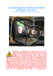
Figure 3-4: Wishbone Bus Connection Diagram
30
Figure 3-4 shows a diagram of the connection between the Wishbone bus and
the CPU. The CPU needed to pass three values: a valid address, the write
enable signal and valid data. The write enable signal was used to determine if it
was a write operation (write enable = 1) or a read operation (write enable = 0).
The CPU only needed to pass valid data in the case of a write operation.
The Wishbone received the information from the CPU and output the required
signals depending on the operation, as shown in Figure 2-8 and Figure 2-9.
The master requested or transferred the required information from/to the slave.
Because both Wishbone interfaces had sequential logic, a minimum of one
clock cycle delay was added to wait for the operation to finish. Therefore a stall
was needed.
A stall generator was added to the CPU and works in the next way. Whenever
an instruction access an external module (I/O, RAM, etc.), a signal called
io_access will go high to notify the external access. The notification of an
external access set the stall signal to high. Because the decoding of the
instruction was done using combinatorial logic, the stall was set to high before
the update of the registers, stopping the execution and preventing
advancement to the next instruction. The stall generation continuously
monitored the Wishbone acknowledgement and strobe signal, waiting for the
end of the bus cycle indicating that the communication exchange was finished.
The Wishbone Bus can be used to access both the I/O Module and the RAM
Module, the decoding to decide which module is address works by checking
the 2 most significant bit of the address; if any bit is a 1 the address is meant
for the I/O Module else is for the RAM, the remaining 14 bits will be used to
address the respective module. The use of 2 bits allows future addition of
different I/O Modules.
3.2.6 System Integration
The last step of the implementation was connecting the stack processor with a
peripheral to test the correct communication using the Wishbone bus. Before
31
this point, the design was not organized with a proper hierarchy, therefore the
next hierarchy was chosen. The purpose of this restructuring was to simplify
the testing, debugging and integration to the design flow.
Figure 3-5: Stack Processor Hierarchy
Figure 3-5 shows the hierarchy organization used for the assignment. The goal
of the hierarchy was to provide modularity and flexibility, allowing the project
the opportunity to use a different RAM module or connect to a different
peripheral in the future using the same code. The CPU had both the Data
Stack and the Return Stack each in an individual module separated from the
logic of the processor.
The peripheral shown in Figure 3-5 was implemented by adding a register file
to the Wishbone Slave interface. A delay generator was also added to the slave
interface, to generate scenarios in which the slaves needed to stall the CPU
multiple clock cycles.
Finally, all elements of the design were connected together, creating the final
design for this assignment. All of the final code can be found in Appendix 7.1.
32
3.3 Testing Process
The present chapter explains the testing used throughout the design process
and the testing done in the final design. A simple overview can be seen in the
Methodology section of Chapter 3.
The base of all testing done in the assignment was the set of instructions
shown in Appendix 7.3. If the expected behavior of an instruction was known,
then the wave form of a design simulation could be compared to the expected
behavior. If any discrepancies exist, then the modification needed to be
inserted into the design. This process was done with every instruction, giving
the basis for the final design obtained on this assignment.
The initial testing used in the assignment was done by simply hardcoding in the
Verilog memory files and simulating them using the RTL design. This process
was slow and repetitive so the decision was made to create a test flow and a
script to make the process more practical and less time consuming.
The first step to do this was to develop custom assembly code for the
processor using Arch C. This allowed easier reading of the code and simplified
the testing overall. The resulting assembler instructions can be found in
Appendix 7.3.
Two types of files were needed to run the testing flow as shown in Figure 3-6.
The RTL files which contained the design of the processor in Verilog code, and
the assembly file which contained the instructions that needed to be executed
along with the expected result of the processor registers. The assembly file was
already written in the custom assembly implemented using Arch C.
Next, the RTL files were compiled using Icarus Iverilog [14], creating an
executable file. The assembly file was compiled to get a Verilog memory file
(.vmem). Both the executable and the VMEM file were used to run the
simulation.
33
Figure 3-6: Testing Flow Diagram
The simulation created two files: a Log file and a Value Change Dumb file
(VCD). The Log file contained the registers values at the end of the simulation.
This file was compared with the initial assembly file to determine if the
instruction execution finished as expected. If not, an error was indicated. The
VCD was used for debugging. It could be opened using the GTKwave and the
waveforms could be analyzed to find any discrepancies or bugs.
Every instruction was tested individually with a specific test. To make testing
even faster, a script was made to run every instruction test with a single
command. The resulting testing flow had the advantage of being automated in
34
a simple flow. On the down side, it did not cover the corner cases, was not
exhaustive, nor was it randomized.
3.4 Synthesis Process
The synthesis let us move from the RTL code to a netlist of gates. This section
first covers the synthesis flow used in the assignment. The RAM connection to
the system can vary for different targets, such as for an FPGA or an ASIC. The
difference between these two synthesis possibilities and the original design are
also discussed.
The synthesis process used the tool Design Compiler by Synopsis. A TCL
script was used to automate and simplify the process. As shown in Figure 3-7,
Design Compiler needed at least three input documents to be able to generate
the required outputs:

RTL Code: Verilog files (.v) that describe the processor architecture and
the design overall.

Libraries: Consisting of a .lib file and a .db file; together they describe
all the standard cells to be used for the synthesis and the information
needed for the RAM and I/O modules if used.

Timing Constraints File: Define the timing requirements the system
needs to fulfill. It also includes the definition of the clock and the clock
period.
The previous inputs were given to the Design Compiler tool and it was able to
perform the synthesis. The result of the synthesis were three files: a report, the
netlist and a constraints file (.sdc). The last two were used as arguments for the
Place and Route process. The report had information about the synthesis and
was used to verify a proper synthesis process was carried out.
35
Figure 3-7: Synthesis Flow
The second part of this section focuses on the different possibilities in which
the RAM could be connected, depending on the target of the synthesis. The
original design had a single dual port RAM that was used for both Program and
Data Memory, as shown in Figure 3-8. For the ASIC implementation, the dual
port RAM had to be replaced by two single port RAMs: one for the program
memory and the other for the data memory.
The needed modifications where made to the RTL code to create the possibility
of toggling between the original design and the ASIC design. A third possibility
was to implement an FPGA Design that used two dual port RAMs, separating
Data and Program memory but using the second port in every RAM for
debugging. This last possibility has not been implemented and will be
discussed in Section 5.
36
Figure 3-8: Different RAM Connections
37
3.5 Place and Route Process
To perform the last step in the implementation, the tool Encounter from
Cadence was used. As with previous steps, a design flow and script were used
to automate and simplify the process.
Figure 3-9: Place and Route Flow
The place and route flow used at Atmel is explained in the steps below using
Figure 3-9 as a reference:
1. Setup: The LIB file and LEF file are in charge of the setup. The LIB file
provides the timing information of the cells. The Library Exchange
Format (LEF) file contains the physical view, pin layout, metal layers and
abstract information of the cells.
2. Read Netlist: The netlist generated by the synthesis process is used as
the input.
38
3. Floor Planning: The first distribution of the chip is made and the die
size and core area are determined. Other blocks, like RAM or I/O
Buffers, are also placed in this step.
4. Power Supply Definition: Depending on the configuration the
characteristics of the power supply are determined. For example, the
decision between using rings or stripes for the power supply is made in
this step.
5. Timing Constraint Reading: The SDC file generated by the synthesis
is used to determine timing limitations and rules.
6. Placement: The first placement is done, driven by timing.
7. Clock-Tree Building: This step uses the clock tree definition file as a
reference.
8. Optimization: An optional optimization step exists before the routing.
9. Routing:
The process of routing cause changes, such as buffer
insertion or timing modification.
10. Optimization: This step will try to fix any timing problems generated by
the Routing.
11. Generate: The last step generates three files:
a. Netlist
b. Standard Parasitic Exchange Format (SPEF) File : File that
contains timing information of the design
c. Design Exchange Format (DEF) File: File representing the
layout of the design.
The last step generates the files needed to do a timing and power analysis,
however, due to time constraints, these were not performed for this
assignment. The process is discussed in Section 5.
39
4 Results
The goal of this section is to show the final design of the assignment, the
modifications to the original design and the results obtained with the final
design.
4.1 Final Design
The final stack processor system was synthetized to target an ASIC module.
The final system architecture diagram can be seen in Figure 4-1.
Figure 4-1: Final Design Architecture
The main change from the original design was the change of a Dual Port RAM
for two Single Port RAMs that separate the Data Memory and the Program
Memory. The separation of the Data Stack and Return Stack into separate
modules was done in the design process. Originally, the stacks would be part
of the CPU logic.
Tasks 1 through 4 from Section 1.3 were completed successfully. The stack
processor system was implemented: designed, tested, simulated, synthetized
41
and place and route was performed. Even though not in the assignment tasks,
a practical test flow was created for the system.
The implemented stack processor is able to successfully execute all the
instruction types mentioned in Section 3.2.3 and in the Appendix 7.3. The
system is capable of communicating with the implemented I/O modules using
the Wishbone Bus using single read and write 16-bit operations; this will be
demonstrated in Section 4.2. The system was designed to simplify the addition
of new instructions.
4.2 Simulations
Some basic instruction execution is shown to demonstrate the proper behavior
of the system. The first case consisted of pushing values to the stack using
Literal type instructions and then doing an ALU addition instruction.
Figure 4-2 shows the waveform resulting from the simulation of the addition
test. Most signals are self-explanatory with the exception of _st0 (New Top of
Stack), st0 (Top of Stack), st1 (Next After Top of Stack) and dsp (Data Stack
Pointer).
The first part of the simulation that needs to be noticed are the reset and start
signals. Execution will not start until start_signal has been asserted. The
instructions of the test are:
lit
lit
lit
add
halt
4
1
10
(0x8004)
(0x8001)
(08x00A)
(0x6203)
(0x6010)
Basically the values 4, 1 and 10 are pushed to stack and then the last two
values are added. It is important to remember that whenever a value is pushed
to the stack, it must to pass through the Top of Stack (st0) and Next After Top
of Stack (st1), because only after going to these two registers will the value be
stored on the stack. As soon as the add instruction is read (0x6203) when the
42
program counter (pc) has a value of 3, the new top of stack is calculated( _st0),
and in the next clock cycle the top of stack (st0) value is updated correctly.
It is important to notice the data stack’s first two positions, data_stack_0 and
data_stack_1, are filled with the value 0. This is due to the fact that whenever
an instruction that will access the stack is executed, the data stack pointer
(dsp) is increased and the value of next of stack (st1) is stored in the data stack
location pointed by the data stack pointer.
Figure 4-2: Add Simulation
During the initialization, the value of st1 is 0 because no value has gone
through the top of stack and therefore the first two locations on the data stack
have value of 0. The first locations of the data stack that are filled with zeroes
due to this behavior will still work properly and be used by the architecture. This
will not affect the proper execution of instructions or the behavior of the
processor.
A hard coded solution could be made by using the drop instruction at the
beginning of a program if starting from position 0 of the data stack is completely
necessary.
43
All ALU instructions had similar satisfactory behaviors, so showing examples of
each one of them is not shown. Instead an example of a CALL instruction is
shown next, covering the proper capability of the processor to do address
modifications.
Figure 4-3 shows the wave form of the simulation of the CALL instruction test.
The instructions of the test are:
lit
call
halt
lit
lit
lit
lit
exit
lit
halt
4
5
6
7
8
9
10
15
(0x8004)
(0x4005)
(0x6010)
(0x8006)
(0x8007)
(0x8008)
(0x8009)
(0x700C)
(0x800A)
(0x6010)
Figure 4-3: Call Simulation
The goal of the test is to use the CALL instruction to jump to a specific part of
the code, and then return with the EXIT instruction. The CALL instruction stores
the return address in the return registers. A behavior similar to the data stack
takes place. The first location to be used in the return stack is not location zero
44
due to the updating of the Return Stack Pointer (rsp). By monitoring the signal
of Top of Stack (st0) and the Program Counter (pc), it is possible to see how
the CALL instruction modifies the pc to jump to the respective program address
and the previous address is stored in the return stack; the value is logically
shifted left once before been store, therefore the value stored in return_stack_1
is the value 4, which is 2 logically shifted left. The program returns to the
original address after using the EXIT instruction. The instruction that pushes
the values 6 and 7 are jumped and the instruction that pushes the value 10 is
not executed, showing the program returning to the correct location in time.
The JUMP and CONDITIONAL JUMP instruction types had similar successful
behavior and their waveforms are not shown.
The communication between the CPU and the peripheral using single read and
write operations with the Wishbone was completed successfully in two cases:
with delay from the slave and without delay from the slave. Figure 4-4 shows a
case in which the communication between master and slaves has no delay.
The test writes the value 4 to the first address register of the I/O module, after
this the value from the first address register is read to verify that the content is
correct. Remember the decoding used by the design uses the top 2 bits of the
address to check which module is addressed, that’s why the value used is
49152 (1100 0000 0000 in binary). The test instructions are the next:
lit
lit
mem_wr
lit
mem_rd
halt
4
49152
49152
15
(0x8004)
(0xC000)
(0x6123)
(0xC000)
(0x6C01)
(0x6010)
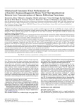
Figure 4-4 signals can be divided in 3 categories from top to bottom: signals
from the CPU, signals from the Wishbone Bus master module and signals from
Wishbone Bus slave module; every segment starts with the modules clock. The
simulation shows the same signal activity as seen in Figure 2-8 and Figure 2-9
when doing a signal write and read operation. The strobe signal (stb_o) and
45
cycle signal (cyc_o) are set high at the start of an external access and will wait
for
the
acknowledgement
signal
(ack_i).
After
receiving
the
first
acknowledgment the value 4 is wrote in the register reg_f0. The value is then
successfully read and wrote to top of stack (st0).
Figure 4-4: Wishbone Bus Communication Example
46
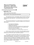
4.3 Area Distribution and Layout
Due to confidentiality reasons with Atmel, only the area distribution of the final
design is shared, as seen in Figure 4-5. The area used for the CPU logic is
minimal, in comparison to the rest of the system. An image of the final place
and route can be seen in Figure 4-6.
Area Distribution
Peripheral
5%
CPU
2%
Program RAM
42%
Data Stack
5%
Return Stack
5%
Data RAM
41%
Figure 4-5: Area Distribution
It is important to remember that the present assignment needed to create a
solid base for future projects and to enable the next user to continue work as
easily as possible. It should be considered that not only was an architecture
implementation made, but also the test flow, the custom assembler and the
documentation needed to follow and repeat the process from step one all the
way to Place and Route were created.
47
Figure 4-6: Place and Route
48
5 Discussion & Future Work
This section discusses the results of the assignment as well as some topics for
future work and optimization. The main tasks of the assignment were
completed successfully. Due to time limitations, the power analysis was not
covered in this assignment. Working on this assignment included a learning
curve adapting to the methodology used by the company. The design, testing,
synthesis and place and route process had to be automated using scripts. This
assignment required the understanding of an elaborate design flow used by
Atmel; learning to use the design flow and incorporating the final design to it
took time.
The original design evolved through the assignment and changed accordingly
in response to the testing process. Overall, a successful implementation of the
stack processor system was achieved. Some suggestions covering possibilities
for future work and optimization of the final design follow.
5.1 Power Analysis
For a future proper power analysis several steps after the place and route
process are required in order to get useful information. Figure 5-1 shows some
of the steps that need to take place after the Place and Route. A back
annotated simulation flow checks if any design changes or constraints are
violated by changes done in the Place and Route and Synthesis process. The
back annotated simulation would use the netlist of the Place and Route and the
SPEF file with the timing constrains generated by the Place and Route.
A power analysis should be done in parallel with a timing analysis using the
same netlist and timing constraints. Finally, for a successful power analysis,
correct stimulation is needed. This can be given using a Switching Activity
Interchange Format (SAIF) file, which contains the toggling activity of all the
signals in the system. Generating clock trees and clock gating configurations
will have an important role in power analysis. This opens many possibilities for
49
testing and comparison. For these reasons, it is considered that this could be
part of another assignment and was not covered by this assignment.
Figure 5-1: Post-Place and Route Flow
5.2 Stack Merging
A possibility was discussed at the end of the assignment to merge the Data
Stack and the Return Stack. This possibility would enable a more compact
architecture, but it would also have some new challenges:

Arbiter: A module in charge of arbitration should be implemented to
avoid cases in which multiple stack accesses are made.

Pointers: The pointers for both stacks would need to be monitored or
modified to not use illegal stack locations.

Delay: This modification would add a possible delay in cases that
consecutive access to the stack is needed.
As shown in Figure 5-2, the arbiter would need to determine which access is
done to the stack and generate a stall if needed.
50
Figure 5-2: Stack Merging
5.3 Wishbone Bus Extension
Even though successful single read and write 16-bit operations are possible
with the actual implementation, the Wishbone Bus could be extended further to
be capable to do advance pipeline communication and burst communication.
The actual Wishbone bus implementation only uses the required signals for
simple communication, no signals providing information of the data transferred
are used; this signals could also be implemented in future work.
The design had specific problems when a back to back I/O access was done in
which the first access tried to read and the second to write to the same location
from an external I/O Module. Possible solutions for this corner case could be
obtained by modifying the stall module in cpu.v or the signals from the
Wishbone Bus modules.
5.4 Pipeline Optimization
The final design has two pipeline stages: the first one consists exclusively of
the fetch stage and the second one consists of the decoding, execution and
51
write back stages of the common pipeline. One possible change that could
improve the behavior of the stack processor system is to move a small part of
the decoding process to the first stage of the pipeline. As shown in Figure 5-3,
adding a small portion of the decoding to the first pipelining fetch could result in
a faster processor and prevent errors from corner cases.
Figure 5-3: Pipeline Modification
52
6 References
[1]
Dave Evans, "The Internet of Things: How the Next Evolution of the
Internet Is Changing Everythin," CISCO IBSG, Apr. 2011. [Online].
http://www.cisco.com/web/about/ac79/docs/innov/IoT_IBSG_0411
FINAL.pdf
[2]
Jim Drew, "Energy Harvesting Produces Power from Local
Enviroment, Eliminating Batteries in Wireless Sensors," Linear
Technology,
Design
Notes
2010.[Online]
http://cds.linear.com/docs/en/design-note/DN483.pdf
[3]
Charles Eric LaForest, "Second-Generation Stack Computer
Architecture," University of Waterloo, Waterloo, 2007. [Online]
Available:http://www.eecg.utoronto.ca/~laforest/SecondGeneration_Stack_Computer_Architecture.pdf
[4]
Jr. Philip J. Koopman, Stack Computers: the new wave. Pittsburgh,
USA: Ellis Horwood, 1989.
[5]
Dr. Klaus Samelson Dr. Friedrich Ludwig Bauer, "Verfahren zur
automatischen
Verarbeitung
von
kodierten
Daten
und
Rechenmaschine zur Ausübung des Verfahrens ," Munich, 1957.
[Online]
http://worldwide.espacenet.com/publicationDetails/originalDocume
nt?CC=DE&NR=1094019&KC=&FT=E
[6]
James
Bowman.
(2009)
The
J1
Forth
CPU.
[Online].
http://www.excamera.com/sphinx/fpga-j1.html
[7]
James
Bowman.
(2010)
www.excamera.com.
[Online].
http://www.excamera.com/files/j1.pdf
[8]
OpenCores.
(2010)
www.opencores.org.
[Online].
http://cdn.opencores.org/downloads/wbspec_b4.pdf
[9]
The ArchC Team, "The ArchC Architecture Description Language
v2.0 ," The ArchC Team, Campinas, Brazil, Reference Manual
53
2007. [Online] http://archc.sourceforge.net/doc.html
[10]
The ArchC Team, "the ArchC Language Suppirt & Tools for
Automatic Generation of Binary Utilities v2.1 ," The ArchC Team,
User Manual 2011. [Online] http://archc.sourceforge.net/doc.html
[11]
The
ArchC
Team.
(2008)
Arch
C.
[Online].
http://archc.sourceforge.net/
[12]
Free Software Fundation. (1998) GNU Operating System. [Online].
http://www.gnu.org/software/emacs/
[13]
Don Ho. (2011) Notepad++. [Online]. http://notepad-plus-plus.org/
[14]
Stephen
Williams.
(2005)
Icarus
Verilog.
[Online].
http://iverilog.icarus.com/
[15]
sourceforge.net.
(2014)
Welcome
toGTKWave.
[Online].
http://gtkwave.sourceforge.net/
[16]
Synopsys.
(2014)
Design
Compiler
2010.
[Online].
http://www.synopsys.com/Tools/Implementation/RTLSynthesis/Des
ignCompiler/Pages/default.aspx
[17]
Cadence Design Systems. (2014) Encounter RTL Compiler.
[Online].
http://www.cadence.com/products/ld/rtl_compiler/pages/default.asp
x
[18]
Chris Bailey Mark Shannon, "Global Stack Allocation," University of
York,
2006.
[Online]
http://www.complang.tuwien.ac.at/anton/euroforth2006/papers/sha
nnon.pdf
54
7 Appendix
7.1 Final RTL Code
The most relevant parts of codes will be shown in this part of the appendix, all the
other code will be added in the digital appendix for practical purposes.
7.1.1 CPU
module cpu (/*AUTOARG*/
// Outputs
read_data, io_access,instr_addr, io_wr, io_addr,io_dout,
// Inputs
ram_addr, clk, cs, reset,io_din,instr,ramrd,ack_i,stb_i
);
`include "stkpc_params.v"
input [4:0] ram_addr; //Ram_address
input
clk;
//Clock
input
reset;
//Reset
input
cs;
//Chip select
input [STKPC_WORD_MSB:0]
io_din;
//I/O Data in
input
[STKPC_WORD_MSB:0]
instr;
//Instruction from Ram
input [STKPC_WORD_MSB:0]
ramrd;
//Ram read input
input
ack_i;
//Wishbone acknowledge signal
input
stb_i;
//Wishbone strobe to signal valid cycle
output
output
output
output
output
output
[STKPC_INST_MSB:0] read_data; //For test bench
[STKPC_PC_MSB:0]
instr_addr;//Next instruction address
io_wr;
// 1= IO Write 0= IO Read
io_access;
// Signal access to IO for WB
[STKPC_WORD_MSB:0] io_addr;
//Output address to IO/RAM
[STKPC_WORD_MSB:0] io_dout;
//Output data to IO/RAM
//Signals for monitoring data and return stack
//ALU Regs//////////////////////////////////////////////
reg [STKPC_WORD_MSB:0]
alu_a;
reg [STKPC_WORD_MSB:0]
alu_b;
wire[STKPC_WORD_MSB:0]
alu_c;
//Data Stack Regs////////////////////////////////////////
reg [STKPC_DSTACK_POINTER_MSB:0]
dsp; //Data stack pointer
reg [STKPC_DSTACK_POINTER_MSB:0]
_dsp; //New data stack pointer
reg [STKPC_DSTACK_MSB:0]
st0; //Top of stack data (T)
55
reg [STKPC_DSTACK_MSB:0]
reg dstkW;
wire _dstkW;
wire[STKPC_DSTACK_MSB:0]
_st0; //New top of stack data (T')
//Data stack write enable Reg
//Data stack write enable
st1 ; //Next of Stack
//Return Stack Regs////////////////////////////////////v
reg [STKPC_RSTACK_MSB:0]
rsp; //Return stack pointer
reg [STKPC_RSTACK_MSB:0]
_rsp; //New return stack pointer
reg
rstkW; //R stack write enable
reg [STKPC_RSTACK_MSB:0]
_rstkD;//Newest return stack data
wire[STKPC_RSTACK_MSB:0]
rst0; //Top of Return stack
//General Regs////////////////////////////////////////
reg [STKPC_PC_MSB:0]
pc;
//Program counter
reg [STKPC_PC_MSB:0]
_pc;
//New program counter
reg [STKPC_PC_MSB:0]
start_signal;//Start Signal
reg
stall;//Stall signal for IO/RAM Access
reg [STKPC_PC_MSB:0]
_instr_addr;//Next instruction address
reg
r_io_access;
//IO Access Reg
reg
halt;
//Halt signal
reg
halt_r;
//Halt Reg
reg
ioWE;
//IO/RAM write enable Reg
wire
_io_access;
//IO Access Signal
wire
_ioWE;
//IO/RAM write enable
wire [STKPC_PC_MSB:0] pc_plus_1; //PC+1 to fetch next instruction
wire [STKPC_WORD_MSB:0]
ramrd;
//Ram read input
//Assigns //////////////////////////////////////////////////
assign
_ioWE =ioWE;
assign
_dstkW=dstkW;
assign
instr_addr =_instr_addr;//Pass addr of next instruction
assign
_io_access=r_io_access;
assign
pc_plus_1 = pc + 1;
assign
io_wr = _ioWE;
//I/O and Ram write enable
assign
io_addr = st0;
//We use top of stack(T) as address
assign
io_dout = st1;
//We use next in stack(N) as data
assign
io_access = (_io_access& stall); //High if access to IO
assign
read_data = instr;
//Every time a instr is taken from
RAM, read_data is updated
//MUX SELECTS////////////////////////////////////////////////
reg [STKPC_SEL_PC_MSB:0]
next_pc_mux_sel;
reg [STKPC_SEL_ALU_A_MSB:0]
alu_a_mux_sel;
reg [STKPC_SEL_ALU_B_MSB:0]
alu_b_mux_sel;
reg [STKPC_SEL_DSP_MSB:0]
dsp_mux_sel;
reg [STKPC_SEL_RSP_MSB:0]
rsp_mux_sel;
reg [STKPC_SEL_RSTACK_MSB :0]
rstack_mux_sel;
reg [STKPC_SEL_ST0_NEW_MSB:0]
_st0_mux_sel;
reg [STKPC_SEL_ALUOP_MSB:0]
alu_op_mux_sel;
reg [STKPC_FLOW_HALT_MSB:0]
halt_mux_sel;
//Stall Generator////////////////////////////////////////////////
56
always @(*) begin
if (reset==1)begin
stall <=0;
end
if (ack_i == 1 | _io_access == 0) begin
stall<=0;
end
else if ((stb_i ==1 | _io_access == 1) && ack_i == 0) begin
stall <= 1;
end
end
// If stall we stay in actual instruction
always @(*) begin
if (stall==1) begin
_instr_addr <= pc;
end
else begin
_instr_addr <= _pc;
end
end
//MUX for PC//////////////////////////////////////////////
always @(*) begin
if (start_signal ==0) begin
//We wait for start signal
_pc <= 0;
end
else begin
case(next_pc_mux_sel)
STKPC_SEL_PC_COND_JMP: begin // Conditional Jump
if (st0==0) begin//If top of stack =0, jump
_pc <= instr[STKPC_ALU_TO_PC_MSB:0];
end
else begin
_pc <= pc_plus_1;
end
end
STKPC_SEL_PC_INC: begin
//PC increment
_pc <= pc_plus_1;
end
STKPC_SEL_PC_INSTR: begin //JMP or CALL
_pc <= instr[STKPC_ALU_TO_PC_MSB:0];
end
STKPC_SEL_PC_RSTACK: begin //EXIT of a routine
_pc <=rst0[STKPC_RSTACK_PC_MSB:STKPC_RSTACK_PC_LSB];
end
default:
_pc <= pc;
endcase
end
end
//MUX for ALU A//////////////////////////////////////VVVV
always @* begin
57
if (start_signal ==0) begin //We wait for start signal
alu_a <= 0;
end
else begin
case(alu_a_mux_sel)
STKPC_SEL_ALU_A_ST0: begin
//Top of data stack
alu_a <= st0;
end
STKPC_SEL_ALU_A_ST1: begin //Next of data stack
alu_a <= st1;
end
STKPC_SEL_ALU_A_RST0: begin //Top of return stack
alu_a <= rst0;
end
STKPC_SEL_ALU_A_RSP: begin //Pointer to return
stack, for checking stack depth
alu_a <= _rsp << 8;
//Shift right to display
rsp in high bits and dsp in low bits
end
default:
alu_a <= alu_a;
endcase
end
end
//MUX for ALU B////////////////////////////////////////
always @* begin
if (start_signal ==0) begin //We wait for start signal
alu_b <= 0;
end
else begin
case(alu_b_mux_sel)
STKPC_SEL_ALU_B_ZERO: begin
//Zeros
alu_b <= STKPC_ZERO_16BITS ;
end
STKPC_SEL_ALU_B_ONES: begin
alu_b <= STKPC_ONES_16BITS; //Ones
end
STKPC_SEL_ALU_B_ST0: begin //Next of data stack
alu_b <= st0;
end
STKPC_SEL_ALU_B_DSP: begin //Data stack pointer
alu_b <= _dsp;
end
default:
alu_b <= alu_b;
endcase
end
end
//MUX for DSP//////////////////////////////////////////////
always @* begin
if (start_signal ==0) begin //We wait for start signal
_dsp <= 0;
end
58
else begin
case(dsp_mux_sel)
STKPC_SEL_DSP: begin
_dsp <= dsp;
end
STKPC_SEL_DSP_INC_1: begin
_dsp <= dsp + 1;
end
STKPC_SEL_DSP_INC_2: begin
_dsp <= dsp + 2;
end
STKPC_SEL_DSP_DEC_1: begin
_dsp <= dsp - 1;
end
default:
_dsp <= dsp;
endcase
end
end
//MUX for RSP//////////////////////////////////////////////////
always @* begin
if (start_signal ==0) begin //We wait for start signal
_rsp <= 0;
end
else begin
case(rsp_mux_sel)
STKPC_SEL_RSP: begin
_rsp <= rsp;
end
STKPC_SEL_RSP_INC_1: begin
_rsp <= rsp + 1;
end
STKPC_SEL_RSP_INC_2: begin
_rsp <= rsp + 2;
end
STKPC_SEL_RSP_DEC_1: begin
_rsp <= rsp - 1;
end
default:
_rsp <= rsp;
endcase
end
end
//MUX for Return Stack//////////////////////////////////////
always @* begin
if (start_signal ==0) begin
//We wait for start signal
_rstkD <= 0;
end
else begin
case(rstack_mux_sel)
STKPC_SEL_RSTACK_PC: begin
_rstkD <= _pc;
59
end
STKPC_SEL_RSTACK_ST0: begin
_rstkD <= st0;
end
STKPC_SEL_RSTACK_PC_PLUS_1: begin
_rstkD <= {pc_plus_1[STKPC_PC_MSB:0], 1'b0};
end
default:
_rstkD <= _pc;
endcase
end
end
//MUX for _ST0//////////////////////////////////
always @(*) begin
if (start_signal ==0) begin
_st0<=0;
end
else begin
case(_st0_mux_sel)
STKPC_SEL_ST0_NEW_ALU: begin
_st0 <= alu_c;
end
STKPC_SEL_ST0_NEW_RAM_IO: begin
_st0 <= |st0[15:14] ? io_din : ramrd;
end
STKPC_SEL_ST0_NEW_IMM: begin
_st0 <= { 1'b0, instr[STKPC_IMM_MSB:0] };
end
default:
_st0 <= st0;
endcase
end
end
// Halt instruction
always @* begin
case(halt_mux_sel)
STKPC_FLOW_HALT_YES: begin
halt = 1'b1;
end
STKPC_FLOW_HALT_NO: begin
halt = 1'b0;
end
default:
halt = 1'b0;
endcase
end
//Instruction Decoder
always @* begin
next_pc_mux_sel=0;
alu_a_mux_sel=0;
60
alu_b_mux_sel=0;
alu_op_mux_sel=0;
dsp_mux_sel=0;
rsp_mux_sel=0;
rstack_mux_sel=0;
_st0_mux_sel=0;
halt_mux_sel = 0;
rstkW=0;
dstkW=0;
ioWE=0;
r_io_access=0;
casez(instr)
STKPC_OPCODES_LIT: begin
next_pc_mux_sel=STKPC_SEL_PC_INC;
alu_a_mux_sel=STKPC_SEL_ALU_A_ST0;
alu_b_mux_sel=STKPC_SEL_ALU_B_ZERO;
alu_op_mux_sel=STKPC_SEL_ALUOP_OR;
dsp_mux_sel=STKPC_SEL_DSP_INC_1;
rsp_mux_sel=STKPC_SEL_RSP;
rstack_mux_sel=STKPC_SEL_RSTACK_PC;
_st0_mux_sel=STKPC_SEL_ST0_NEW_IMM;
halt_mux_sel = STKPC_FLOW_HALT_NO;
rstkW=0;
dstkW=1;
ioWE=0;
r_io_access=0;
end
STKPC_OPCODES_JMP: begin
next_pc_mux_sel=STKPC_SEL_PC_INSTR;
alu_a_mux_sel=STKPC_SEL_ALU_A_ST0;
alu_b_mux_sel=STKPC_SEL_ALU_B_ZERO;
alu_op_mux_sel=STKPC_SEL_ALUOP_OR;
dsp_mux_sel=STKPC_SEL_DSP;
rsp_mux_sel=STKPC_SEL_RSP;
rstack_mux_sel=STKPC_SEL_RSTACK_PC;
_st0_mux_sel=STKPC_SEL_ST0_NEW_ALU;
halt_mux_sel = STKPC_FLOW_HALT_NO;
rstkW=0;
dstkW=0;
ioWE=0;
r_io_access=0;
end
//all instructions were decoded as the previous 2 examples, for
practical purposes other instructions will be removed from the
written document, please refer to the digital appendix for th full
list.
endcase
end
//Data Stack//////////////////////////////////////
data_stack DATA_STACK (
61
// Outputs
.data_out
// Inputs
.data_in
.addr_rd
.addr_wr
.wr_en
.clk
(st1),
(st0),
(dsp),
(_dsp),
(_dstkW),
(clk)
);
//Return Stack////////////////////////////
return_stack RETURN_STACK (
// Outputs
.data_out
(rst0),
// Inputs
.data_in
(_rstkD),
.addr_rd
(rsp),
.addr_wr
(_rsp),
.wr_en
(rstkW),
.clk
(clk)
);
//ALU////////////////////////////////////
stkpc_alu STKPC_ALU (
// Outputs
.c
(alu_c[STKPC_WORD_MSB:0]),
// Inputs
.a
(alu_a[STKPC_WORD_MSB:0]),
.b
(alu_b[STKPC_WORD_MSB:0]),
.op
(alu_op_mux_sel[STKPC_SEL_ALUOP_MSB:0])
);
//Update PC, pointers////////////////////////
always @(posedge clk or posedge reset) begin
if (reset==1'b1) begin
pc <= 0;
dsp <= 0;
st0 <= 0;
rsp <= 0;
halt_r <=0;
end else if(stall==0) begin
dsp <= _dsp;
pc <= _pc;
st0 <= _st0;
rsp <= _rsp;
halt_r <= halt;
end
end
//start signal to initiate after initial reset
always @(posedge clk or posedge reset) begin
if (reset==1'b1) begin
62
start_signal<=0;
end else begin
start_signal <=1;
end
end
endmodule //cpu
7.1.2 Dual Port Ram
module ram2ports (/*AUTOARG*/
// Outputs
data_out_a,data_out_b,
// Inputs
clock, addr_a, addr_b, data_in_a,data_in_b, cs_a, we_a, cs_b, we_b
);
parameter WORD_WIDTH = 16;
parameter ADDR_WIDTH = 8;
parameter RAM_SIZE = 1<< ADDR_WIDTH;
localparam WORD_MSB = WORD_WIDTH-1;
localparam ADDR_MSB = ADDR_WIDTH-1;
output [WORD_MSB:0] data_out_a;
output [WORD_MSB:0] data_out_b;
input clock;
//Port A
input [ADDR_MSB:0]
input [WORD_MSB:0]
input
input
//Port B
input [ADDR_MSB:0]
input [WORD_MSB:0]
input
input
reg
reg
reg
reg
reg
[WORD_MSB:0]
[WORD_MSB:0]
[WORD_MSB:0]
[ADDR_MSB:0]
[ADDR_MSB:0]
addr_a;
data_in_a;
cs_a;
we_a;
addr_b;
data_in_b;
cs_b;
we_b;
data_out_a;
data_out_b;
mem0 [0:RAM_SIZE-1];
addr_a_latched;
addr_b_latched;
event dbg_addr_a;
//Update of address latches
always @(posedge clock) begin
if(cs_a) begin
addr_a_latched <= addr_a;
end
if(cs_b) begin
addr_b_latched <= addr_b;
end
end
63
//Update of data out of port a
always @(addr_a_latched) begin
-> dbg_addr_a;
data_out_a <= mem0[addr_a_latched[ADDR_MSB:0]];
end
//Update of data out of port a
always @(addr_b_latched) begin
data_out_b <= mem0[addr_b_latched[ADDR_MSB:0]];
end
// Write
always @(posedge clock) begin
if(cs_a && we_a) begin
$display("Memory write A ");
mem0[addr_a] <= data_in_a;
end
if(cs_b && we_b) begin
$display("Memory write B");
mem0[addr_b] <= data_in_b;
end
end
endmodule // ram2ports
7.1.3 Data Stack
module data_stack (
// Outputs
data_out,data_stack_0,data_stack_1,data_stack_2,data_stack_3,data_st
ack_4,data_stack_5,data_stack_6,data_stack_7,data_stack_8,
// Inputs
data_in,addr_rd,addr_wr,rd_en,wr_en,clk
);
`include "stkpc_params.v"
//Outputs
output[STKPC_WORD_MSB:0]
data_out;
output [STKPC_DSTACK_MSB:0] data_stack_0; //Signals to monitor
content of data stack, 7 more registers are used but omitted of the
printed version for practical purposes.
//Inputs
input [STKPC_WORD_MSB:0]
data_in;
input [STKPC_DSTACK_POINTER_MSB:0]
addr_rd;
input [STKPC_DSTACK_POINTER_MSB:0]
addr_wr;
input
rd_en;
input
wr_en;
input
clk;
assign data_stack_0
reg [STKPC_WORD_MSB:0]
= dstack[0];
data_out;
64
reg [STKPC_DSTACK_MSB:0]
dstack[0:STKPC_DSTACK_SIZE]; //Data stack
//update of data and return stack, pushing the top of stack
always @(posedge clk ) begin
if (wr_en) begin
dstack[addr_wr] = data_in;
end
end
always@(*) begin
data_out<= dstack[addr_rd];
end
endmodule
7.1.4 Return Stack
module return_stack (
// Outputs
data_out,return_stack_0,return_stack_1,return_stack_2,
// Inputs
data_in,addr_rd,addr_wr,rd_en,wr_en,clk
);
`include "stkpc_params.v"
//Outputs
output[STKPC_WORD_MSB:0]
output [STKPC_RSTACK_MSB:0]
output [STKPC_RSTACK_MSB:0]
output [STKPC_RSTACK_MSB:0]
//Inputs
input [STKPC_WORD_MSB:0]
input [STKPC_WORD_MSB:0]
input [STKPC_WORD_MSB:0]
input
input
input
assign return_stack_0
assign return_stack_1
assign return_stack_2
data_out;
return_stack_0; use to monitor stack
return_stack_1;
return_stack_2;
data_in;
addr_rd;
addr_wr;
rd_en;
wr_en;
clk;
= rstack[0];
= rstack[1];
= rstack[2];
reg [STKPC_WORD_MSB:0]
reg [STKPC_RSTACK_MSB:0]
data_out;
rstack[0:STKPC_RSTACK_SIZE];//Return stack
//update of data and return stack, pushing the top of stack
always @(posedge clk) begin
if (wr_en) begin
rstack[addr_wr] = data_in;
end
end
always@(*) begin
65
data_out<= rstack[addr_rd];
end
endmodule
7.1.5 Wishbone Master Module
module wb_m_16 (
// Outputs
adr_o, dat_o, we_o, sel_o, stb_o, cyc_o,dat_i_cpu,
// Inputs
rst_i,clk_i,dat_i,ack_i,err_i,rty_i,dat_o_cpu,adr_o_cpu,
we_i_cpu,cs,io_access
);
`include "stkpc_params.v"
//Outputs
output[WB_ADR_O_MSB:0]
output[WB_DAT_O_MSB:0]
output
output[WB_SEL_O_MSB:0]
output
output
output[WB_DAT_O_MSB:0]
WB module
adr_o;
dat_o;
we_o;
sel_o;
stb_o;
cyc_o;
dat_i_cpu;
//Inputs
input
input
input
[WB_DAT_I_MSB:0]
input
input
input
input
[WB_DAT_O_MSB:0]
input
[WB_ADR_O_MSB:0]
Module
input
WB Module
input
input
reg [WB_ADR_O_MSB:0]
reg [WB_DAT_O_MSB:0]
reg
reg[WB_SEL_O_MSB:0]
reg
reg
reg[WB_DAT_O_MSB:0]
//WB Signals
//Address Out
//Data Out
//Write/Read Enable
//Select Out
//Strobe Signal
//Cycle Signal
//Data send to CPU received from
rst_i;
clk_i;
dat_i;
ack_i;
err_i;
rty_i;
dat_o_cpu;
adr_o_cpu;
//WB Signals
//Reset
//Clock
//Data In
//Acknowledgement Out
//Error Signal
//Retry Signal
//Data from CPU to WB Module
//Address from CPU to WB
we_i_cpu;
//Enable signal from CPU to
cs;
io_access;
//Chip Select
//IO_Access Signal
adr_o;
dat_o;
we_o;
sel_o;
stb_o;
cyc_o;
dat_i_cpu;
66
wire
_io_access;
assign _io_access = io_access|stb_o;
//Every IO Access we update the data out, the address and write
enable
always @ (*) begin
if (io_access ==1) begin
adr_o <= adr_o_cpu;
dat_o <= dat_o_cpu;
end
end
//The data from the WB bus is passed to the CPU
always @(*) begin
dat_i_cpu<=dat_i;
end
always @ (*) begin
if (io_access ==1 && we_i_cpu ==1) begin
we_o <=we_i_cpu;
end else if(io_access ==1 && we_i_cpu ==0) begin
we_o <=we_i_cpu;
end
end
always @(posedge clk_i ) begin
if(rst_i==1'b1) begin
stb_o <= 0;
cyc_o <=0;
end
else begin
if (io_access==1 && ack_i==0) begin //If slave is free,
cycle start
sel_o[0]<= 1;
cyc_o <= 1;
stb_o <=1;
end else if ( ack_i==1) begin //If slave is done finish
cycle
stb_o <= 0;
cyc_o <= 0;
end
end
end
endmodule // wb_m_16
7.1.6 Wishbone Slave Module
module wb_s_16 (/*AUTOARG*/
// Outputs
67
dat_o,ack_o,err_o,rty_o,reg_f0,reg_f1,reg_f2,reg_f3,reg_f4,reg_f5,
// Inputs
rst_i,clk_i,dat_i,adr_i,cyc_i,we_i,stb_i,sel_i,cs
);
`include "stkpc_params.v"
//Outputs
output[WB_DAT_O_MSB:0]
output
output
output
design
output[WB_DAT_O_MSB:0]
register file
output[WB_DAT_O_MSB:0]
output[WB_DAT_O_MSB:0]
output[WB_DAT_O_MSB:0]
output[WB_DAT_O_MSB:0]
output[WB_DAT_O_MSB:0]
dat_o;
ack_o;
rty_o;
err_o;
//WB Signals
//Data out
//Acknowledgement out
//Ready out
//Error out, not used for simple
reg_f0; //Outputs used to monitor the
reg_f1;
reg_f2;
reg_f3;
reg_f4;
reg_f5;
//Inputs
input
rst_i;
input
clk_i;
input
[WB_DAT_O_MSB:0]
dat_i;
input
[WB_ADR_O_MSB:0]
adr_i;
input
cyc_i;
cycle is in progress if high
input
we_i;
input
stb_i;
input
[WB_SEL_O_MSB:0]
sel_i;
input
cs;
//WB Signals
//Reset
//Clock
//Data in
//Address in
//Cycle input, to notifies a
//Write enable
//Strobe in
//Select in
//Chip select
reg [WB_DAT_O_MSB:0]
reg_file [0:GPIO_REG_FILE_MSB];
//Register file to store data
reg [WB_DAT_O_MSB:0]
dat_o;
reg
rty_o;
reg
err_o;
reg [WB_DELAY_MSB:0]
temp_count; //Temporal to count cycles
reg
ready;
//Signal to notify that
slave finish its processing and can transmit back
reg
wire
//Used
assign
assign
assign
assign
assign
assign
assign
assign
r_ack_o;
_ack_o;
to monitor register file in simulation
reg_f0 = reg_file[0];
reg_f1 = reg_file[1];
reg_f2 = reg_file[2];
reg_f3 = reg_file[3];
reg_f4 = reg_file[4];
reg_f5 = reg_file[5];
_ack_o = r_ack_o;
ack_o = _ack_o & stb_i;
68
wire [WB_DELAY_MSB:0]
wcet; //Worst case execution time, max
cycles of delay needed for slave operation
assign wcet = 'd0;
//Delay generator
always @(posedge clk_i or posedge rst_i) begin
if(rst_i == 1'b1) begin
ready <= 0;
temp_count <= 0;
end
else begin
if (stb_i==1) begin
temp_count <= temp_count+1;
if (temp_count == wcet) begin
ready <= 1;
temp_count <= 0;
end
end
else begin
temp_count <= 0;
ready <= 0;
end
end
end
//Data in and out
always @(posedge clk_i or posedge rst_i) begin
if(rst_i==1'b1) begin
dat_o <= 0;
r_ack_o <= 0;
rty_o <= 0;
err_o <= 0;
end else if(cs) begin
//If WB is the target
if(wcet==0) begin
if (we_i==0 && stb_i==1) begin //Master is going to read
dat_o<= reg_file[adr_i&255];
r_ack_o<= 1;
end else if (we_i == 1 && stb_i == 1 ) begin //Write
reg_file[adr_i&255]<= dat_i;
r_ack_o<= 1;
end else begin //if we are reading and slave is ready
r_ack_o<=0;
end
end
else begin
if (we_i==0 && stb_i==1&& ready ==1) begin //Read
dat_o<= reg_file[adr_i&255];
r_ack_o<= 1;
end else if (we_i == 1 && stb_i == 1 && ready == 1) begin
//Master is going to write
reg_file[adr_i&255]<= dat_i;
r_ack_o<= 1;
end else begin
//if we are reading and
slave is ready
69
r_ack_o<=0;
end
end
end
end
endmodule //wb_s_16
7.2 ArchC Files
7.2.1 Stkpc.ac
//@begin[arch_ac]
AC_ARCH(stkpc) {
ac_mem
DM:5M;
ac_regbank RB:15;
ac_reg new_st0;
ac_reg st0;
ac_reg st1;
ac_reg rst0;
ac_wordsize 16;
ARCH_CTOR(stkpc) {
ac_isa("stkpc_isa.ac");
set_endian("little");
};
};
//@end[arch_ac]
7.2.2 Stkpc_isa.ac
AC_ISA(stkpc){
//@begin[inst_format]
ac_format
ac_format
ac_format
ac_format
ac_format
Type_Lit = "%opcode1:1 %uk15:15 ";
Type_Jmp = "%opcode1:1 %opcode2:2 %uk13:13 ";
Type_Cond_Jmp = "%opcode1:1 %opcode2:2 %uk13:13 ";
Type_Call = "%opcode1:1 %opcode2:2 %uk13:13 ";
Type_Alu = "%opcode1:1 %opcode2:2 %opcode3:13 ";
//@end[inst_format]
//@begin[inst_list]
ac_instr<Type_Lit> lit;
ac_instr<Type_Jmp> jmp;
ac_instr<Type_Cond_Jmp> cond_jmp;
ac_instr<Type_Call> call;
70
ac_instr<Type_Alu>
nop,halt,nip,exit,dup,rs_push,swap,over,drop,mem_wr,add,and,or,xor,i
nvert,n_eq_t,n_lt_t,n_sr_t,sub1,rs_pop,rs_cp,mem_rd,n_sl_t,stk_dep,n
_ult_t;
//@end[inst_list]
// gas MIPS specific register names
ac_asm_map reg {
"r"[0..14] = [0..14];
}
//@begin[ac_isa_sreg]
ac_asm_map sreg {
"new_st0" = 8;
"st0" = 9;
"st1" = 10;
"rst0" = 0;
}
//@end[ac_isa_sreg]
ISA_CTOR(stkpc){
//@begin[ac_set_asm]
lit.set_asm("lit %exp", uk15);
lit.set_decoder(opcode1=1);
jmp.set_asm("jmp %exp", uk13);
jmp.set_decoder(opcode1=0,opcode2=0);
cond_jmp.set_asm("cond_jmp %exp", uk13);
cond_jmp.set_decoder(opcode1=0,opcode2=1);
call.set_asm("call %exp", uk13);
call.set_decoder(opcode1=0,opcode2=2);
nop.set_asm("nop");
nop.set_decoder(opcode1=0,opcode2=3,opcode3=0);
halt.set_asm("halt");
halt.set_decoder(opcode1=0,opcode2=3,opcode3=16);
nip.set_asm("nip");
nip.set_decoder(opcode1=0,opcode2=3,opcode3=3);
exit.set_asm("exit");
exit.set_decoder(opcode1=0,opcode2=3,opcode3=4108);
dup.set_asm("dup");
dup.set_decoder(opcode1=0,opcode2=3,opcode3=129);
rs_push.set_asm("rs_push");
rs_push.set_decoder(opcode1=0,opcode2=3,opcode3=327);
swap.set_asm("swap");
71
swap.set_decoder(opcode1=0,opcode2=3,opcode3=384);
over.set_asm("over");
over.set_decoder(opcode1=0,opcode2=3,opcode3=385);
drop.set_asm("drop");
drop.set_decoder(opcode1=0,opcode2=3,opcode3=259);
mem_wr.set_asm("mem_wr");
mem_wr.set_decoder(opcode1=0,opcode2=3,opcode3=291);
add.set_asm("add");
add.set_decoder(opcode1=0,opcode2=3,opcode3=515);
and.set_asm("and");
and.set_decoder(opcode1=0,opcode2=3,opcode3=771);
or.set_asm("or");
or.set_decoder(opcode1=0,opcode2=3,opcode3=1027);
xor.set_asm("xor");
xor.set_decoder(opcode1=0,opcode2=3,opcode3=1283);
invert.set_asm("invert");
invert.set_decoder(opcode1=0,opcode2=3,opcode3=1539);
n_eq_t.set_asm("n_eq_t");
n_eq_t.set_decoder(opcode1=0,opcode2=3,opcode3=1795);
n_lt_t.set_asm("n_lt_t");
n_lt_t.set_decoder(opcode1=0,opcode2=3,opcode3=2051);
n_sr_t.set_asm("n_sr_t");
n_sr_t.set_decoder(opcode1=0,opcode2=3,opcode3=2307);
sub1.set_asm("sub1");
sub1.set_decoder(opcode1=0,opcode2=3,opcode3=2563);
rs_pop.set_asm("rs_pop");
rs_pop.set_decoder(opcode1=0,opcode2=3,opcode3=2957);
rs_cp.set_asm("rs_cp");
rs_cp.set_decoder(opcode1=0,opcode2=3,opcode3=2945);
mem_rd.set_asm("mem_rd");
mem_rd.set_decoder(opcode1=0,opcode2=3,opcode3=3073);
n_sl_t.set_asm("n_sl_t");
n_sl_t.set_decoder(opcode1=0,opcode2=3,opcode3=3331);
stk_dep.set_asm("stk_dep");
stk_dep.set_decoder(opcode1=0,opcode2=3,opcode3=3584);
n_ult_t.set_asm("n_ult_t");
72
n_ult_t.set_decoder(opcode1=0,opcode2=3,opcode3=3843);
};
};
7.3 Instruction Set Table
For a complete description of each instruction and instruction type please refer to
the digital Appendix.
Name
Assembler
Instruction
Description
Type
lit
Literal
Load 15 bit value to top of
stack
Jump
jmp
Jump
Jump to given PC value
Conditional
cond_jmp
Conditional
Jumps to given PC value, if
Top of stack equal zero
Literal
Operation
Jump
Jump
Call
call
Call
Addition
add
ALU
Logical And
and
ALU
Logical Or
or
ALU
Logical Xor
xor
ALU
Drop
drop
ALU
Duplicate
dup
ALU
Exit
exit
ALU
Invert
invert
ALU
Memory Read
mem_rd
ALU
Jumps to given PC value
and old PC value is saved
in return stack
16 bit addition of the 2 top
values of data stack
16 bit and operation of the
2 top values of data stack
16 bit or operation of the 2
top values of data stack
16 bit xor operation of the 2
top values of data stack
Drops top value of the data
stack
Duplicate top value of the
data stack
Jumps to PC taken from
the top of the return stack
Bitwise logic invert of the
top of stack
Read to external module
Memory Write
mem_wr
ALU
Write to an external module
Equal
comparator
n_eq_t
ALU
No operation
nop
ALU
Returns a 0 if 2 top values
of data stack are different,
else returns 0xFFFF
no operation
73
Less Than
n_lt_t
ALU
n_sl_t
ALU
m_sr_t
ALU
Unsigned
Less Than
n_ult_t
ALU
Over
operation
over
ALU
Logical
Left
Shift
Logical Right
Shift
Return Stack
Copy
Return Stack
Push
Return Stack
Pop
Stack Depth
rs_cp
ALU
rs_push
ALU
rs_pop
ALU
stk_dep
ALU
Swap
Operation
swap
ALU
Subtract One
sub1
ALU
Returns 0xFFFF if second
of data stack is smaller
than top of stack, else
returns 0
Second of data stack is
shifted left by value given
by top of stack
Second of data stack is
shifted right by value given
by top of stack
Returns 0xFFFF if second
of data stack is smaller
than top of stack, else
returns 0. Uses unsigned
values
Value in second of data
stack is copied to the top of
stack.
Copies the top of return
stack to top of data stack
Push value of top of data
stack to return stack
Drop top of return stack
Top of stack is given the
value of the data stack
pointer in the top 8 bits,
and the value of the return
stack pointer in the 8 lower
bits
Swaps the second of data
stack with the top of data
stack
Subtracts 1 of top of data
stack.
74