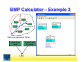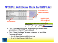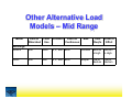
1
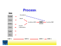
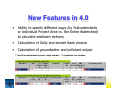
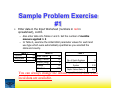
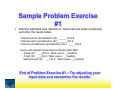
GRTS Model Training
US EPA: Andrea Matzke ([email protected])
Tetra Tech: Sabu Paul ([email protected])
What Will You Learn?
• STEPL model
1. Create an Excel Model
2. Use BMP calculator
• R5 model (a simple Excel model not just
for Region 5)
• Special discussion
– BMP Efficiency Estimator
– Online data server
Part 1: STEPL
What is STEPL?
• Calculates nutrient (N, P, and BOD pollutants)
and sediment loads by land use type and
aggregated by watershed
• Calculates load reductions as a result of
implementing BMPs
• Data driven and highly empirical
• A customized MS Excel spreadsheet model
– Simple and easy to use
– Formulas and default parameter values can be
modified by users (optional) with no programming
required
STEPL Users?
• Basic understanding of hydrology, erosion, and
pollutant loading processes
• Knowledge (use and limitation) of
environmental data (e.g., land use, agricultural
statistics, and BMP efficiencies)
• Familiarity with MS Excel and Excel Formulas
Process
Sources
Groundwater
Cropland
Runoff
Urban
Load before BMP
BMP
Load after BMP
Pasture
Forest
Erosion/
Sedimentation
Feedlot
Others
STEP 1
STEP 2
STEP 3
STEP 4
STEPL Web Site
Link to on-line
Data server
Link to download
setup program to
install STEPL program
and documents
Temporary URL: http://it.tetratech-ffx.com/stepl until moved to EPA server
STEPL Main Program
• Run STEPL executable program to create
and customize spreadsheet dynamically
STEPL Spreadsheet
Composed of four worksheets
BMPs Worksheet
Each land use type within each watershed can have a separate BMP.
Also it can be partial application.
Total Load Worksheet
Each row of results corresponds to a different watershed or project.
Graphs Worksheet
STEPL BMP Calculator
• Calculates combined efficiency of a BMP train for a
given land use. The use of BMP calculator requires the
understanding of BMPs and their placement in the
Series
Reduced tillage
watershed.
Parallel
Conventional
tillage
Reduced tillage
Filter strip
Conventional
tillage
Reduced tillage
Settling Basin
Combination
Customized Menu
Tip: To ensure that files are linked to the customized
menu, set Excel Default file location to C\STEPL or
D:\STEPL
Step: Tools menu > Options submenu> General tab
STEPL BMP Calculator
• Describe schematically BMP configuration
– Number and linkages
– BMP type and efficiency
– Land use area
Use source area or
original load as the
weighting factor
Delete Connection
• Calculate combined
efficiency
Add BMP box
Draw Connection
Calculate combined
efficiency
Move BMP box
New Features in 4.0
•
Ability to specify different ways (by Subwatersheds
or Individual Project Area vs. the Entire Watershed)
to calculate sediment delivery
•
Calculation of Gully and stream bank erosion
•
Calculation of groundwater and pollutant output
Hands-on Exercises
Sample Problem Exercises
• Exercise #1
– Estimate total annual load for a specific farm, and total load
reduction resulting to implementation of a (single) BMP on
croplands
• Hypothetical watersheds based on Agricultural Statistics and NRCS data
• Exercise #2
– Similar to Exercise #1 but with multiple BMPs
• Exercise #3
– Similar to Exercise #1 but BMP trains implemented on croplands,
and a single BMP on urban land
• Exercise #4
– Similar to Exercise #1 but for multiple subwatersheds and BMP
trains implemented on croplands, and pasture land
• Exercise #5
– Hypothetical watersheds for demonstrating gully and streambank
erosion
Sample Problem Exercise
#1
Estimate total annual load for a farm
in Cullman County in Alabama
Cullman
County
Agricultural Statistics of Alabama
Based on 2002 Census of Agriculture, USDA National Agricultural
Statistics Service
Agricultural Statistics of Cullman County
Land Information
Average Farm Size (ac)
101
Average Cropland Size (ac)
64.2
Animal Information
Animal
Total
Average
Beef Cattle
39,018
28.58
Dairy Cattle
1,962
140.14
Swine (Hog)
152
11.69
Sheep
508
25.4
Chicken
1,572,552 14427.08
Based on 2002 Census of Agriculture, USDA National Agricultural
Statistics Service
•
Sample Problem Exercise
#1
Generate a new custom spreadsheet. Note that you may reuse
a spreadsheet you created previously for a different project.
– Click Start button (e.g., normally located at the Windows bottom
left corner), then Program, STEPL, and STEPL to run the STEPL
main executable program (stepl.exe in /STEPL folder) and display
main interface
– Select options. For Exercise #1, specify the following:
• Specify number of watershed = 1
• Select first option under Option for Initialization (default selection – Set
initial land use areas and animal numbers to zeros)
– Click ok to create new spreadsheet
– Click ok to the following message box
– Save the spreadsheet using a new file name
• For this example, you may save it to exercise1.xls
– When the new spreadsheet is opened, click Ok button to enable
stored formulas/equations in the spreadsheet
•
Sample Problem Exercise
#1
Enter data in the Input Worksheet (numbers in red in
spreadsheet)
– By default, optional tables are not shown. Click yes to show
the optional tables (Table 5-8) with their default values. Click
no to hide them.
– Select state = Alabama, and county = Cullman. Notice that
initial values for Annual Rainfall and Number of Rain Days are
automatically specified in Table 1 as you select a state or
county.
– Select a weather station = Al Birmingham FAA. Notice that
correction factors change with the selected weather station.
– In Table 1, enter the land use areas for your watershed (Refer
next slide)
– Also in Table 1, Select the feedlot percent paved assuming
feedlot area is not zero. Default value = 0-24%.
Sample Problem Exercise
#1
•
Enter data in the Input Worksheet (numbers in red in
spreadsheet), cont’d.
– Also enter data into Tables 2 and 3. Set the number of months
manure applied to 3
– In Table 4, examine the initial USLE parameter values for each land
use type which were automatically specified as you selected the
state and county.
Table 1
Cropland
Pastureland
Feedlots
Table 2
75
Beef Cattle
20
5 Dairy Cattle
Swine (Hog)
Sheep
Chicken
Table 3
10
10
5
10
100
No. of Septic Systems
Population per Septic
System
2.38
Septic Failure Rate, %
0.87
5
You can always change the default and initial data when
local data are available.
•
Sample Problem Exercise
#1
Examine estimated load in Total Load and Graph worksheets
and enter the results below:
Total Annual N Load (lb/yr): ________ 4699.1
Total Annual P Load (lb/yr): ________ 1042.7
Total Annual Sediment Load (ton/yr): ________ 428.5
Amount and source with highest annual load contribution:
N load (lb/yr): __2276.2.0 What source: ___ Cropland
P load (lb/yr): __705.6 What source: ___ Cropland
Sediment load (lb/yr): _406.1 What source: ___ Cropland
Note that load reduction = 0 since you have not specified
any BMP yet – see next slide
Sample Problem Exercise #1
For the same farm area, estimate total
annual load reduction assuming reduced
tillage is practiced in cropland areas
• Enter BMP data in BMPs worksheet
– In Table 1 which is for cropland areas, select
Reduced Tillage System under BMP column. Note
that initial values of BMP efficiencies are
automatically specified with the selected BMP.
Sample Problem Exercise
#1
•
Examine estimated load reduction in Total Load and Graph worksheets
and enter the results below:
Total Annual N Load Reduction (lb): ______ 1511.8
Total Annual P Load Reduction (lb): _______467.6
Total Annual Sediment Load Reduction (ton): _____304.6
Source with highest annual load contribution after BMP:
N load (lb): ___2135.9 What source: __Feedlots
P load (lb): ___292.9 What source: __ Feedlots
Sediment load (lb): ___101.5 What source: __Cropland
End of Problem Exercise #1 – Try adjusting your
input data and reexamine the results.
Sample Problem Exercise
#1
•
•
In the Input worksheet check the box next to Groundwater
load calculation
Examine estimated load in Total Load and Graph worksheets and
enter the results below:
Total Annual N Load (lb/yr): ________ 5221.0
Total Annual P Load (lb/yr): ________ 1065.2
Total Annual Sediment Load (ton/yr): ________ 428.5
Amount and source with highest annual load contribution:
N load (lb/yr): __2135.92 What source: ___ Feedlot
P load (lb/yr): __292.95 What source: ___ Feedlot
Sediment load (lb/yr): _101.52 What source: ___ Cropland
End of Problem Exercise #1 – Try adjusting your
input data and reexamine the results.
Sample Problem Exercise
#2
For the same farm area, estimate total annual
load reduction assuming reduced tillage is
practiced in cropland areas and Solids
Separation Basin BMP on feedlots
• Create a spreadsheet for this project or exercise.
– Instead of generating a new custom spreadsheet using the
STEPL main executable program, you will be using the
spreadsheet in the previous exercise.
– Save the spreadsheet used for Exercise #1 to save recent
changes.
– Save this spreadsheet with a new name (exercise2.xls, be
sure to save the file as *.xls type). This new
spreadsheet will be used for Exercise #2.
Sample Problem Exercise
#2
• Enter new data in the Input Worksheet
– Note that all the input data entered in the previous spreadsheet are
still valid
– Only modification is an additional BMP
•
Sample Problem Exercise
#2
Examine estimated load reduction in Total Load and Graph
worksheets and enter the results below:
Total Annual N Load Reduction (lb): ____2259.4
Total Annual P Load Reduction (lb): _____ 558.4
Total Annual Sediment Load Reduction (ton): ____ 304.6
Source with highest annual load contribution after BMP:
N load (lb): _1388.3 What source: __Feedlots
P load (lb): _237.97 What source: __Cropland
Sediment load (lb): _101.5 What source: __Cropland
Note that load reductions have been calculated since BMPs have been already
specified in the previous exercise. For this exercise, assume that the same BMPs
are installed for all cropland and urban areas in the 8-digit watershed.
Sample Problem Exercise
#3
Estimate total annual load and load reduction for a watershed that
consists more than one farm where all croplands are practicing
reduced tillage and filter strips (shown below) and urban open
spaces has LID/Bioretention:
Reduced tillage
Filter strip
Assume all croplands is implementing
the above BMP train
Sample Problem Exercise
#3
• Create a spreadsheet for this project or
exercise.
– Save the spreadsheet used in Exercise #2 to
exercise3.xls.
– Enter new data in the Input Worksheet
Sample Problem Exercise
#3
• Examine estimated load in Total Load and Graph worksheets
and enter the results below:
Total Annual N Load (lb): ____17015.2
Total Annual P Load (lb): ____ 4108.5
Total Annual Sediment Load (ton): ___ 1526.7
Source with highest annual load contribution:
N load (lb): __11208.3 What source: ___Cropland
P load (lb): __3176.6 What source: ____Cropland
Sediment load (lb): __1467.7 What source: __Cropland
Sample Problem Exercise
#3
• Enter BMP data in BMP worksheet
– In Table 1, which is for cropland areas, select “CombinedBMP calculated” under BMP column to indicate that we have
a “Reduced Tillage-Filter Strip” BMP train in croplands.
– Note that the N, P, BOD, and Sediment BMP efficiencies
remained zero. If you have the combined efficiency values
for this particular BMP train, enter them in Table 7 (number
in red). These values will be reflected in Table 1 and in
other tables (i.e., if the same BMP train is implemented for
other land uses).
– If you do not have the values, you may use the BMP
calculator (next step)
•
Sample Problem Exercise
#3
Use BMP Calculator to estimate combined efficiencies
of the BMP train
– Run the BMP Calculator by selecting the STEPL/BMP
Calculator menu of the STEPL spreadsheet. If the
system cannot find the BMP Calculator program,
navigate to /STEPL folder and select BMPCalculator.exe
– Using the BMP Calculator interface, do the following
(refer back to slide 13 for steps in using BMP
Calculator):
• Add two BMP boxes (one each for Reduced Tillage, and
Filter Strip)
• Enter BMP information (type, area, etc.) for each BMP box
by double-clicking the box (Question: What is the area
associated with the filter strip)
• Specify the connection between the two BMPs (Question:
Which BMP should be upstream). You may move the
boxes to make them more readable
• Calculate the combined efficiencies for N, P, BOD, and
Sediment (0.865, 0.863, ND, 0.913).
• Enter the combined efficiencies in Table 7 of STEPL
spreadsheet. Note the efficiencies are reflected in Table 1.
Sample Problem Exercise #3
• Click Urban BMP Tool
– Select Open Space under urban land use options->Select
LID/Bioretention under Available LID/BMP -> Click Apply
LID/BMP
You can always manually change the initial BMP efficiencies
if local data are available.
If your BMP is not in the selection list, you may use STEPL-View/Edit BMP
List menu to add your BMP to the database (please refer to the user manual)
•
Sample Problem Exercise
#3
Examine estimated load reduction in Total Load and
Graph worksheets and enter the results below:
Total Annual N Load Reduction (lb): ___9929.3
Total Annual P Load Reduction (lb): ____ 2833.4
Total Annual Sediment Reduction (ton): ____ 1340.0
Source with highest annual load contribution after BMP:
N load (lb): __3952.4 What source: __ Feedlot
P load (lb): __658.6 What source: __Feedlot
Sediment load (lb): __127.7 What source: __Cropland
End of Problem Exercise #3 – Try adjusting your
input data and reexamine the results.
Sample Problem Exercise
#4
• Generate a new custom spreadsheet.
– Similar to exercise 1 create a new spreadsheet, but specify
two watersheds this time ( Program-> STEPL-> STEPL)
– Select options. For Exercise #4, specify the following:
• Specify number of watershed = 2
• Select first option under Option for Initialization (default
selection – Set initial land use areas and animal numbers to
zeros)
– Click ok to create new spreadsheet
– Click ok to the following message box
– Save the spreadsheet using a new file name
• For this example, you may save it to exercise4.xls
– When the new spreadsheet is opened, click Ok button to
enable stored formulas/equations in the spreadsheet
Sample Problem Exercise
#4
• Enter data in the Input Worksheet
(numbers in red in spreadsheet)
– Select state = Alabama, and county =
Cullman.
– Select a weather station = Al Birmingham
FAA.
Sample Problem Exercise
#4
• Enter data in the Input Worksheet
(numbers in red in spreadsheet), cont’d
Sample Problem Exercise
#4
• Cropland in watershed 1 has the same BMP train as in
example 2,
• Cropland in watershed 2 has filter strip
• Pastureland in both watersheds has filter strip
Reduced tillage
Filter strip
Assume all croplands in watershed 1 is implementing
the above BMP train
Sample Problem Exercise
#4
• Cropland in watershed 1 has the same BMP train as in
example 2,
• Cropland in watershed 2 has filter strip
• Pastureland in both watersheds has filter strip
•
Sample Problem Exercise
#4
Examine estimated load reduction in Total Load and
Graph worksheets and enter the results below:
Total Annual N Load Reduction (lb): ___ 6909.5
Total Annual P Load Reduction (lb): ____ 1920.5
Total Annual Sediment Reduction (ton): ____ 980.3
Source with highest annual load contribution after BMP:
N load (lb): __2844.1 What source: __ Feedlot
P load (lb): __528.7 What source: __Cropland
Sediment load (lb): __287.6 What source: __Cropland
•
Sample Problem Exercise
#4
In the Input worksheet, check the box next to Treat all the
subwatersheds as parts of a single watershed.
• Examine estimated load reduction in Total Load and Graph
worksheets and enter the results below:
Total Annual N Load Reduction (lb): ___ 6184.3
Total Annual P Load Reduction (lb): ____ 1641.3
Total Annual Sediment Reduction (ton): ____ 753.6
Source with highest annual load contribution after BMP:
N load (lb): __2844.1 What source: __ Feedlot
P load (lb): __483.79 What source: __Cropland
Sediment load (lb): __351.18 What source: __Cropland
End of Problem Exercise #4 – Try adjusting your
input data and reexamine the results.
•
Sample Problem Exercise
#5
Generate a new custom spreadsheet.
– Similar to exercise 1 create a new spreadsheet, but specify
three watersheds this time ( Program-> STEPL-> STEPL)
– Select options. For Exercise #5, specify the following:
•
•
•
•
Specify number of watershed = 3
Specify gully formations = 2
Specify impaired streambanks = 2
Select second option under Option for Initialization (Test
STEPL model with non-zero initial numbers)
– Click ok to create new spreadsheet
– Click ok to the following message box
– Save the spreadsheet using a new file name
• For this example, you may save it to exercise5.xls
– When the new spreadsheet is opened, click Ok button to
enable stored formulas/equations in the spreadsheet
Sample Problem Exercise
#5
• Enter data in the Input Worksheet
(numbers in red in spreadsheet)
– Select state = Alabama, and county =
Cullman.
– Select a weather station = Al Birmingham
FAA.
Sample Problem Exercise
#5
• Click Gully and Streambank Erosion button in BMPs
Worksheet and enter data in the Gully&Streambank
Worksheet (numbers in red in spreadsheet)
Sample Problem Exercise
#5
• Examine estimated load reduction in Total
Load and Graph worksheets and enter the
results below:
Total Annual N Load Reduction (lb): ___ 20.0
Total Annual P Load Reduction (lb): ____ 7.7
Total Annual Sediment Reduction (ton): ____ 13.8
End of Problem Exercise #5 – Try adjusting your
input data and reexamine the results.
BMP Calculator
More Exercises for BMP
Calculator
•
Try different BMP trains in the BMP Calculator. Note that you may
define as many trains as you want and calculate each BMP train’s
combined efficiency at the same time in the same window. You don’t
need to open a separate BMP window for each BMP train (see
illustration below).
Need of BMP Calculator
• When is BMP Calculator needed?
Not needed - No combined
efficiency calculation
Needed - Each land use type
uses more than one type of BMP
BMP Calculator – Example 1
1
2
3
Each box represents 100 ac
Crop Regular
Tillage
Crop Reduced
Tillage
Filter Strip
Load
BMP Calculator – Example 2
1
3
2
Each box represents 100 ac
Forest Road
Grass Planting
Forest No Onsite Road BMP
Filter Strip
Load
BMP Calculator – Example 3
1
2
3
Each box represents 100 ac
Urban Grass
Swale
Load
Urban Porous
Pavement
Adding BMP Data
Add New Data to BMP List
• In STEPL customized menu, click “View/Edit BMP List”
• BMPList worksheet is shown, add or delete BMPs
Customized menu
Example: New data inserted
here
STEPL: Add New Data to BMP List
Update BMP button
(BMPList worksheet)
New BMP added!
New BMP added!
(BMPs worksheet)
• Click “Update BMP Data” button to update the BMP
selections in the BMPs worksheet
• Click “Save Updates” to save changes to text files
(comma delimited)
– C:or D:\Stepl\Support\AllBMPstepl.csv
– C: or D:\Stepl\Support\AllBMP.csv
Part 2: Region 5 Model
R5 model is not limited to Region
5
If controls of the model does not work, set EXCEL > Tools > Macro >Macros
>Security to Medium
Region 5 model
has five functional
worksheets.
Region 5 Load Estimation Model
• Introduction
– Provide a general estimate of pollutant reduction at the source level
– Initially developed by Indiana Department of Environmental
Management (IDEM) based on Michigan DEQ’s pollution control
manual for section 319 watersheds.
Gully Erosion: Calculate Load Reduction
•
•
Select a soil texture (e.g. sand, loamy sand)
Enter gully dimensions and the number of years since the gully formed
Gully Stabilization
• Load
Average annual erosion during the life of the gully (t/y)
= Volume x Soil Weight / Years
Nutrient load
= Annual Erosion x Soil Nutrient Conc. x Correction Factor
• Load Reduction after implementing gully stabilization
– Specify reduction efficiency (100% efficiency by default)
– Reduction is equal to annual erosion x user-specified efficiency
Volume = (Top Width +Bottom Width) x Depth x Length / 2
Gully Erosion: Nutrient Correction Factor
• Correction Factor
– Smaller soil particles -> larger aggregated surface area -> more
nutrients attached
Soil Texture
Nutrient Correction Factor
Clay
1.15
Silt
1.00
Sand
0.85
Peat
1.50
•
•
Stream Bank Erosion—
Calculation
Select a soil texture (e.g. silty clay)
Enter the dimensions of the eroding stream banks
Stream Bank Erosion
• Load (Channel Erosion)
= Length * Height * Lateral Recession rate * Soil weight
• Load Reduction
= Load * Load reduction efficiency
Determining Lateral Recession Rate by Field Observation
Lateral Recession
Rate (ft/yr)
Category
Description
0.01 – 0.05
Slight
Some bare bank, no
exposed roots
0.06 – 0.2
Moderate
Bank is mostly bare
0.3 – 0.5
Severe
Bank is bare with
exposed roots
Very Severe
Bank is bare with
fallen trees
0.5+
Agricultural Practices—Usage
• Check BMPs: Agricultural field practices and filter strips (check both)
• Select a state and a county for default USLE parameter values
• Modify the default USLE parameter values for local conditions,
especially the cover factor C and the supporting practice factor P to
reflect the before and after treatment effects
Agricultural Practices—Usage 2
• Enter contributing areas (e.g. 50 acres)
• Select a soil texture (e.g. silt)
Note: This worksheet is also applicable to other cases (mining,
construction sites) when USLE is used.
Feedlot Pollution Reduction
•
Load
–
–
–
–
–
Enter a contributing area (e.g. 1.74 acre)
Specify the percentage of paved area (e.g. 75-100%)
Select state and a county (Pennsylvania, Lycoming)
Select Weather Station (NY New York Central Park)
Enter animal count for each type
Feedlot Pollution Reduction
•
Load Reduction
–
–
Select a feedlot best management practice (e.g. waste
management system)
System calculates load reduction using pre-assigned (BOD,
P, N) efficiencies for the selected BMP
Urban Pollution Reduction
•
Load
–
–
Enter size (acres) of storm water sewered and unsewered areas
for each urban land use subclass
System calculates load using default unit loads for each land
use sub class
Note: Storm sewers
Urban Pollution Reduction
•
Load Reduction
–
–
Select BMP
System calculates load using default BMP efficiencies
for the selected BMP
Region 5 model vs. STEPL 1
•
Region 5 model
–
–
•
Calculates load at the source level
Sources are independent (no relationship
between worksheets)
STEPL
–
–
–
–
Calculates load for different sources at
source and watershed level
Sources are related in watershed
User can specify and update BMP list
BMP calculator for complex BMP
arrangements
Part 3: Special Discussion
BMP Efficiency Estimator
• Simple calculator to estimate BMP
efficiency for non structural BMP
• Estimates efficiency due tochanges in
cropping patterns or soil support
practices
BMP Efficiency Estimator –
contd.
Other Alternative Load
Models - Simple
Model
Simple
Simple
Method
FHWA
SLOSS/
PHOSPH
Watershed
Field or
Watershed
Land
Use
Pollutant
Event or
Continuous
BMP
Data
Reqt’s
Level of
Effort
Watershed
Urban
N, P
Event
Low
Low
Both
Both
Urban
Rural
N, P
P, Sed
Event
Event
Low
Low
Low
Low
Both
Both
P
Event
Simple
Medium Medium
Reference: List of alternative load and load reduction models,
STEPL Web site.
Other Alternative Load
Models – Mid Range
Model
Field or
Watershed
Land
Use
Pollutant
Event or
Continuous
BMP
Data
Reqt’s
Level of
Effort
Mid Range
AGNPS
Both
Rural
N, P, Sed Both
Detailed Medium Medium
to High to High
GWLF
Both
Both
N, P, Sed Both
Simple
Low to
Low to
Medium Medium
Other Alternative Load
Models - Detailed
Model
Field or
Watershed
Land
Use
Pollutant
Event or
Continuous
BMP
Data
Reqt’s
Level of
Effort
Detailed/Complex
ANSWERS Both
Rural
N, P, Sed Both
Detailed Medium Medium
to High to High
GLEAMS
Field
Rural
N, P, Sed Both
HSPF
Both
Both
N, P, Sed Both
SWAT
SWMM
WEPP
Both
Both
Both
Rural
Both
Rural
N, P, Sed Both
N, P, Sed Both
Sed
Continuous
Detailed Medium
to High
Detailed Medium
to High
Detailed Medium
Detailed High
Detailed Low to
High
Medium
to High
Medium
to High
Medium
High
Low to
High
STEPL Online Input Data Server
ONLY FOR PRACTICE!!
STEPL Online Input Data Server
Data is available at
HUC and county
intersection (HUCO
Polygon)
Generate data
summaries
Note:
Zoom in further to display polygon IDs
STEPL Online Input Data Server: Basic Report
Data is summarized by HUCO polygon
STEPL: Discussion
• Watershed vs. subwatershed
– STEPL model is not limited to subwatershed (can apply to
farms, scenarios, etc.)
– Watershed size (make the subwatershed small enough to
reflect BMP effectiveness.
– You want to know the reduction at the local subwatershed
level (Sum of loads from subwatersheds ≠ load at the
watershed outlet because of the transport loss in the main
stem.)
•
•
•
•
•
•
•
Local weather data
How to use the user-defined land use?
Septic failure rate clarification
Add new BMPs to the list
Small treated area vs. large watershed
R5 100% efficiency assumptions
Estimate BMP efficiencies using USLE tables
Some useful data!
Estimate BMP Efficiency Using USLE C Value
Table I
Generalized Values of Cover and Management Factor (C) for Field Crops East of the Rocky Mountains (Stewart et al 1975).
Crop, rotation & management b/
Productivity a/
(Please use the abbreviation table below!)
High
Moderate
----------------------------------------------------------------------------------------------------------------Continuous fallow, tilled up and down slope
1.00
1.00
CORN
1
C, RdR, fall TP, conv (1)
0.54
0.62
2
C, RdR, spring TP, conv (1)
0.50
0.59
3
C, RdL, fall TP, conv (1)
0.42
0.52
4
C, RdR, wc seeding, spring TP, conv (1)
0.40
0.49
5
C, RdL, standing, spring TP, conv (1)
0.38
0.48
6
C, fall shred stalks, spring TP, conv (1)
0.35
0.44
7
C(silage)-W(RdL,fall TP) (2)
0.31
0.35
8
C, RdL, fall chisel, spring disk, 40-30% re (1)
0.24
0.30
9
C(silage), W wc seeding, no-till p1 in c-k W (1) 0.20
0.24
10
C(RdL)-W(RdL, spring TP) (2)
0.20
0.28
11
C, fall shred stalks, chisel p1, 40-30% re (1)
0.19
0.26
12
C-C-C-W-M, RdL, TP for C, disk for W (5)
0.17
0.23
13
C, RdL, strip till row zones, 55-40% re (1)
0.16
0.24
14
C-C-C-W-M-M, RdL, TP for C, disk for W (6)
0.14
0.20
15
C-C-W-M, RdL, TP for C, disk for W (4)
0.12
0.17
16
C, fall shred, no-till pl, 70-50% re (1)
0.11
0.18
17
C-C-W-M-M, RdL, TP for C, disk for W (5)
0.087
0.14
18
C-C-C-W-M, RdL, no-till pl 2nd & 3rd C (5)
0.076
0.13
19
C-C-W-M, RdL, no-till pl 2d C (4)
0.068
0.11
20
C, no-till pl in c-k wheat, 90-70% re (1)
0.062
0.14
21
C-C-C-W-M-M, no-till p1 2d & 3rd C (6)
0.061
0.11
22
C-W-M, RdL, TP for C, disk for W (3)
0.055
0.095
23
C-C-W-M-M, RdL, no-till pl 2d C (5)
0.051
0.094
24
C-W-M-M, RdL, TP for C, disk for W (4)
0.039
0.074
25
C-W-M-M-M, RdL, TP for C, disk for W (5)
0.032
0.061
26
C, no-till pl in c-k sod, 95-80% re (1)
0.017
0.053
Estimate BMP Efficiency Using USLE C Value
Table II
Generalized Values of Cover and Management Factor (C) for Field Crops East of the Rocky Mountains (Stewart et al 1975).
Crop, rotation & management b/
Productivity a/
(Please use the abbreviation table below!)
High
Moderate
----------------------------------------------------------------------------------------------------------------COTTON /c
27
Cot, conv (western plains) (1)
0.42
0.49
28
Cot, conv (south) (1)
0.34
0.40
MEADOW (HAY)
29
Grass & legume mix
0.004
0.01
30
Alfalfa, lespedeza or sericia
0.020
31
Sweet clover
0.025
SORGHUM, GRAIN (western plains)
32
RdL, spring TP, conv (1)
0.43
0.53
33
No-till pl in shredded 70-50% re
0.11
0.18
SOYBEANS /c
34
B, RdL, spring TP, conv (1)
0.48
0.54
35
C-B, TP annually, conv (2)
0.43
0.51
36
B, no-till pl
0.22
0.28
37
C-B, no-till pl, fall shred C stalks (2)
0.18
0.22
WHEAT
38
W-F, fall TP after W (2)
0.38
39
W-F, stubble mulch, 500 lb re (2)
0.32
40
W-F, stubble mulch, 1000 lb re (2)
0.21
41
Spring W, RdL, Sept TP, conv (ND,SD) (1)
0.23
42
winter W, RdL, Aug TP, conv (KS) (1)
0.19
43
Spring W, stubble mulch, 750 lb re (1)
0.15
44
Spring W, stubble mulch, 1250 lb re (1)
0.12
45
Winter W, stubble mulch, 750 lb re (1)
0.11
46
Winter W, stubble mulch, 1250 lb re (1)
0.10
47
W-M, conv (2)
0.054
48
W-M-M, conv (3)
0.026
49
W-M-M-M, conv (4)
0.021
--------------------------------------------------------------------------------------------------------------
Estimate BMP Efficiency Using USLE C Value
Table III
Values of Cover and Management Factor (C) for Pasture and Woodland (Novotny & Chesters, 1981).
Cover
Value
-------------------------------------------------------------------------------------------------------Permanent pasture, idle land, unmanaged woodland
95-100% ground cover
as grass
0.003
as weeds
0.01
80% ground cover
as grass
0.01
as weeds
0.04
60% ground cover
as grass
0.04
as weeds
0.09
Managed woodland
75-100% tree canopy
0.001
40-75% tree canopy
0.002-0.004
20-40% tree canopy
0.003-0.01
--------------------------------------------------------------------------------------------------------
For example: Increase ground cover from 60% to
80% will reduce erosion about 75%
Estimate BMP Efficiency Using USLE C Value
Table IV
Generalized Values of Cover and Management Factor (C) for Field Crops East of the Rocky Mountains (Stewart et al 1975).
Notes and Abbreviations
a/. High level exemplified by long-term yield averages greater than 75 bu/ac corn or 3 ton/ac hay or cotton management that regularly
provides good stands and growth.
b/. Numbers in parentheses indicate numbers of years in the rotation cycle. (1) indicates a continuous one-crop system.
c/. Grain sorghum, soybeans or cotton may be substituted for corn in lines 12,14,15, 17-19, 21-25 to estimate values for sod-based
rotations.
Abbreviations:
B
C
c-k
conv
cot
lb re
% re
xx-yy% re
RdR
RdL
TP
soybeans
F
fallow
corn
M
grass & legume hay
chemically killed
pl
plant
conventional
W
wheat
cotton
wc
winter cover
pounds of residue per acre remaining on surface after new crop seeding
percentage of soil surface covered by residue mulch after new crop seeding
xx% cover for high productivity, yy% for moderate
residues (corn stover, straw, etc.) removed or burned
residues left on field (on surface or incorporated)
turn plowed (upper 5 or more inches of soil inverted, covering residues
Estimate BMP Efficiency Using USLE P Value
Table
Values of Supporting Practice Factor (P) (Stewart et al 1975).
Practice Slope(%):
1.1-2
2.1-7
7.1-12
12.1-18
18.1-24
-------------------------------------------------------------------------------------------------------------------------------No support practice
1.00
1.00
1.00
1.00
1.00
Contouring
0.60
0.50
0.60
0.80
0.90
Contour strip cropping
R-R-M-M /a
0.30
0.25
0.30
0.40
0.45
R-W-M-M
0.30
0.25
0.30
0.40
0.45
R-R-W-M
0.45
0.38
0.45
0.60
0.68
R-W
0.52
0.44
0.52
0.70
0.90
R-O
0.60
0.50
0.60
0.80
0.90
Contour listing or
ridge planting
0.30
0.25
0.30
0.40
0.45
½
½
½
½
0.5/n
0.6/n
0.8/n
0.9/n½
Contour terracing /b
0.6/n
a/. R = row crop, W = fall-seeded grain, M = meadow. The crops are grown in rotation and so
arranged on the field that row crop strips are always separated by a meadow or winter-grain strip.
b/. These factors estimate the amount of soil eroded to the terrace channels. To obtain off-field
values, multiply by 0.2. n = number of approximately equal length intervals into which the field slope is
divided by the terraces. Tillage operations must be parallel to the terraces.
For example: Contouring will reduce sediment by 1040% depending on slope
Estimate Runoff Changes Using Curve Number
Runoff Curve Numbers (Antecedent Moisture Condition II) for Cultivated Agricultural Land (Soil Conservation Service, 1986).
Land Use/Cover
Hydrologic Condition
A
B
C
D <- Soil Hydrologic Group
-----------------------------------------------------------------------------------------------------------Fallow Bare Soil
77
86
91
94
Crop residue cover (CR)
Poor *
76
85
90
93
Good
74
83
88
90
Row Crops Straight row (SR) Poor
72
81
88
91
Good
67
78
85
89
SR+CR
Poor
71
80
87
90
Good
64
75
82
85
Contoured (C)
Poor
70
79
84
88
Good
65
75
82
86
C+CR
Poor
69
78
83
87
Good
64
74
81
85
Contoured & terraced (C&T)
Poor
66
74
80
82
Good
62
71
78
81
C&T + CR
Poor
65
73
79
81
Good
61
70
77
80
Small
SR
Poor
65
76
84
88
Grains
Good
63
75
83
87
SR+CR
Poor
64
75
83
86
Good
60
72
80
84
C
Poor
63
74
82
85
Good
61
73
81
84
C+CR
Poor
62
73
81
84
Good
60
72
80
83
C&T
Poor
61
72
79
82
Good
59
70
78
81
C&T + CR
Poor
60
71
78
81
Good
58
69
77
80
CloseSR
Poor
66
77
85
89
seeded or
Good
58
72
81
85
broadcast
C
Poor
64
75
83
85
legumes or
Good
55
69
78
83
rotation
C&T
Poor
63
73
80
83
meadow
Good
51
67
76
80
-------------------------------------------------------------------------------------------------------------
Estimate Runoff Changes Using Curve Number II
Runoff Curve Numbers (Antecedent Moisture Condition II) for Other Rural Land (Soil Conservation Service, 1986).
Hydrologic
Soil Hydrologic
Land Use/Cover
Condition
Group
A
B
C
------------------------------------------------------------------------------------------------------------------------------------------Pasture, grassland or range
Poor/a
68
79
86
- continuous forage for grazing
Fair
49
69
79
Good
39
61
74
Meadow – continuous grass, protected
from grazing, generally mowed for hay
30
58
71
D
89
84
80
78
Brush - brush/weeds/grass mixture
with brush the major element
Poor/b
Fair
Good
48
35
30
67
56
48
77
70
65
83
77
73
Woods/grass combination
(orchard or tree farm) /c
Poor
Fair
Good
57
43
32
73
65
58
82
76
72
86
82
79
Woods
Poor/d
Fair
Good
45
36
30
66
60
55
77
73
70
83
79
77
Farmsteads – buildings, lanes,
driveways and surrounding lots
59
74
82
86
------------------------------------------------------------------------------------------------------------------------------------------a) Poor: 50% ground cover or heavily grazed with no mulch; Fair: 50 to 75% ground cover and not heavily grazed; Good: > 75% ground
cover and lightly or only occasionally grazed.
b) Poor: < 50% ground cover; Fair 50 to 75% ground cover; Good: > 75% ground cover.
c) Estimated as 50% woods, 50% pasture.
d) Poor: forest lifter, small trees and brush are destroyed by heavy grazing or regular burning; Fair: woods are grazed but not burned and
some forest lifter covers the soil; Good: Woods are protected from grazing and litter and brush adequately cover the soil.
Estimate Runoff Changes Using Curve Number III
Runoff Curve Numbers (Antecedent Moisture Condition II) for Arid and Semiarid Rangelands (Soil Conservation Service, 1986).
Hydrologic
Soil Hydrologic
Land Use/Cover
Condition
Group
A
B
C
------------------------------------------------------------------------------------------------------------------------------------------Herbaceous - grass, weeds & lowPoor /a
80
87
growing brush; brush the minor
Fair
71
81
component
Good
62
74
93
89
85
Oak/aspen - oak brush, aspen, Poor
mountain mahogany, bitter brush,
maple and other brush
D
Fair
Good
-
66
48
30
74
57
41
79
63
48
Pinyon/juniper - pinyon, juniper or
both; grass understory
Poor
Fair
Good
-
75
58
41
85
73
61
89
80
71
Sagebrush with grass understory
Poor
Fair
Good
-
67
51
35
80
63
47
85
70
55
Desert scrub - saltbush, greasewood,
Poor
63
77
85
88
creosotebrush, blackbrush, bursage,
Fair
55
72
81
86
palo verde, mesquite and cactus
Good
49
68
79
84
-----------------------------------------------------------------------------------------------------------------------------------a. Poor: < 30% ground cover (litter, grass and brush overstory); Fair: 30 to 70% ground cover; Good: 70% ground cover.
Estimate Runoff Changes Using Curve Number IV
Runoff Curve Numbers (Antecedent Moisture Condition II) for Urban Areas (Soil Conservation Service, 1986).
Hydrologic
Soil Hydrologic
Land Use/Cover
Condition
Group
A
B
C
D
-------------------------------------------------------------------------------------------------------------------------------------------------------Open space (lawns, parks, golf
courses, cemeteries, etc.):
Poor condition (grass cover < 50%)
68
79
86
89
Fair condition (grass cover 50-75%)
49
69
79
84
Good condition (grass cover> 75%)
39
61
74
80
Impervious areas:
Paved parking lots, roofs,
driveways, etc.)
98
98
98
98
Streets and roads:
Paved with curbs & storm sewers
98
98
98
98
Paved with open ditches
83
89
92
93
Gravel
76
85
89
91
Dirt
72
82
87
89
Western desert urban areas:
Natural desert landscaping (pervious
areas, only)
63
77
85
88
Artificial desert landscaping
(impervious weed barrier, desert
shrub with 1-2 in sand or gravel
mulch and basin borders)
96
96
96
96
---------------------------------------------------------------------------------------------------------------------------------------------------------