Download Modeling Protein Interaction Networks with Answer Set Programming

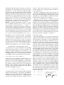
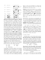
Modeling Protein Interaction Networks with Answer Set Programming
∗ Dept.
Timur Fayruzov∗ , Martine De Cock∗† , Chris Cornelis∗ and Dirk Vermeir‡
of Applied Mathematics and Computer Science, Ghent University, Krijgslaan 281 (S9), 9000 Ghent, Belgium
Email: [email protected]
† Institute of Technology, University of Washington, Tacoma, WA-98402, USA
Email: [email protected]
‡ Department of Computer Science, Vrije Universiteit Brussel, Pleinlaan 2, 1050 Brussels, Belgium
Email: [email protected]
Abstract—In this paper we propose the use of answer set
programming (ASP) to model protein interaction networks.
We argue that this declarative formalism rivals the popular
boolean networks in terms of ease of use, while at the same time
being more expressive. As we demonstrate for the particular
case of a fission yeast network, all information present in a
boolean network, as well as relevant background assumptions,
can be expressed explicitly in an answer set program. Moreover,
readily available answer set solvers can then be used to find
the stable states of the network.
Keywords-Biological system modeling, Logic, Artificial intelligence
I. I NTRODUCTION
With the increasing availability of experimental biological
information, biological systems modeling has become an
important research domain. Existing approaches (see e.g. [5],
[8] for good overviews) can roughly be divided into two
groups. Quantitative models are mostly made up of various
kinds of differential equations, and considerable efforts are
required to build such models. A lot of experimental data,
such as the concentration of different types of molecules at
different time points, is needed. This information is often
very difficult and expensive to obtain.
Qualitative models are less information-demanding, but
less precise as well. However, it turns out that significant
simplifications, such as using a discrete timing and disregarding quantitative information, still allow to model the
behavior of a system correctly. Thus, many efforts have been
made to adopt discrete modeling techniques. Among them,
discrete dynamical networks based on boolean networks are
one of the best established qualitative modeling methods
widely used by biologists to model protein regulation networks (see e.g. [1], [4]). The nodes of a boolean network
represent protein molecules and the directed edges represent
interactions. Edges can be typed to represent different kinds
of interactions, such as inhibition and activation.
While liked for their simplicity, dynamical networks have
the disadvantage of not being self-descriptive, i.e. they
are built under some background assumptions that are not
explicitly stated in the network itself. Furthermore, as explained in Section II-B, their use requires the development
a
a
b
c
(b)
(a)
Figure 1.
b
Examples of boolean networks
of specific algorithms to retrieve the stable states of the
network (see e.g. [9]), and different algorithms can cause
different execution flows.
In this paper, we propose to represent protein interaction
networks by answer set programs [10]. As a first illustration,
Example 1 shows an answer set program corresponding to
the network depicted in Figure 1a. The prefixes G and S are
used to separate general rules from specific rules describing
a particular network. Rules S1-S4 capture all the information
that is present in Figure 1a, namely that a and b are proteins
(rules S1 and S2), that a activates b at any given time T
(rule S3), and likewise that b activates a (rule S4). Rules
S5 and S6 express that in the initial state (time step 0), a is
active while b is not. The G-rules describe a general boolean
network semantics that does not change from network to
network; we refer to Section III for more details.
Example 1 Answer set program P1 for the network in
Figure 1a.
G1 :
G2 :
G3 :
G4 :
G5 :
G6 :
S1 :
S2 :
S3 :
time(0..2).
act(Y, T + 1)
inh(Y, T + 1)
←
←
←
←
←
act(X, T + 1)
inh(X, T + 1)
prot(a).
prot(b).
activates(a, b, T ).
act(X, T ), activates(X, Y, T ).
act(X, T ), inhibits(X, Y, T ).
act(X, T ), inh(X, T ).
act(X, T ), not inh(X, T + 1).
inh(X, T ), not act(X, T + 1).
S4 : activates(b, a, T ).
S5 : act(a, 0).
S6 : inh(b, 0).
As explained below, the answer set of P1 is hact(a,0),
inh(b,0), act(a,1), act(b,1), act(a,2), act(b,2), act(a,3),
act(b,3)i. Here predicates correspond to a protein state at
a corresponding time step. In this answer set there is no
difference between the protein states at time steps 1 and 2.
Hence we conclude that, under the given initial conditions,
the stable state of the system is hact(a), act(b)i. The actual
answer set of the program includes more information that
is not relevant to our task. In our answer set representation
we omit this information for the sake of conciseness.
Note that only network specific rules such as rules S1S6 need to be redefined for a given protein interaction
network, while the other rules model general biological
properties. This makes the representation of such networks
in ASP intuitively simple, while at the same time the ASP
machinery becomes available to analyze and predict the
behavior of the described network at hand. One of the main
advantages of modeling with ASP is that all background
information can and should be expressed explicitly in the
model, while it is implicit in dynamical networks. This also
allows to normalize different networks into one standard
form. Furthermore, the use of ASP eliminates the need for
specific network execution algorithms to retrieve the stable
states of the networks. In fact, another main advantage of
using ASP is that all supporting tools such as solvers and
grounders are readily available. For the results described in
this paper we used the lparse [14] grounder coupled with
the smodels [12] solver, which is a default choice for many
ASP-related tasks.
Our work is not the first attempt to use ASP to model
biological networks. In [2], [6], [15] the authors propose to
use ASP-based action languages to model, query or plan the
execution of biological systems. Our approach, however, is
different in several aspects that are discussed in Section V.
The paper is structured as follows. We begin by recalling
the necessary preliminaries about ASP and boolean networks
in Section II. In Section III we explain in detail how to
describe a protein interaction network as an answer set
program: we develop a framework of general rules (Grules), that describe a general boolean network semantics,
and we give examples of specific rules (S-rules), that allow
a biologist to describe a specific protein interaction network
under study. In Section IV we illustrate our approach on
a fission yeast network, while in Section V we explain its
relationship with existing work. We conclude in Section VI.
II. P RELIMINARIES
a negative literal. Another form of negation that represents
a special feature of ASP, is negation-as-failure (naf) denoted
by not. For instance, rule G5 from Example 1 states that if
protein X is active at time T and there is no evidence that
X becomes inhibited at time T + 1, then X should still be
active at time T + 1.
An answer set program is a set of rules such as program
P1 from Example 1. The set of all literals of a program P is
denoted by LitP . An interpretation of P is any consistent1
subset S ⊆ LitP . S is said to satisfy a rule with a nonempty
head, if {L1 , . . . , Lm } ⊆ S and {Lm+1 , . . . , Ln } ∩ S = ∅
implies that L0 ∈ S. When the head is empty, then
S is said to satisfy the rule if {L1 , . . . , Lm } 6⊆ S or
{Lm+1 , . . . , Ln } ∩ S 6= ∅.
An interpretation that satisfies all rules of a program P
is called a model of P . Answer sets are special kinds of
models. First of all, for a program P without naf, an answer
set of P is a minimal model of P , i.e. S is called an answer
set of P iff S is a model of P and there is no model K
such that K ⊂ S.
Example 2 The models of
a
Answer set programming [10] is a declarative formalism
that allows to express relations between truth values of
propositions with rules of the form
L0
←
L1 , . . . , Lm , not Lm+1 , . . . , not Ln
in which L0 , L1 , . . . , Ln are called literals. The left-hand
side of a rule is called the head, while the right-hand side
is called the body of the rule. A rule with an empty head,
such as rule G4 from Example 1, is called a constraint. A
rule with an empty body is called a fact (rules S1-S6). A
rule intuitively states that whenever literals in the body hold
true, proposition head should be true as well. A literal can
be negated, then it is preceded by the symbol ¬ and is called
b
are ha,bi, hai and ∅. The minimal model is ∅.
The concept of an answer set is extended for the program
P containing negation-as-failure as described below. Suppose that S is a model of P , and our hypothesis is that S is
an answer set of P . In order to check if S is an answer set
of P , we build a reduct program P 0 by 1) removing from
P all rules that contain a naf-literal not L, with L ∈ S; 2)
removing all the naf-literals from the bodies of the remaining
rules. If the minimal model S 0 of the naf-free program P 0
coincides with S, then S is an answer set of the original
program P .
Example 3 A program with negation-as-failure can have
more than one answer set. Suppose that we have one seat
and two persons a and b, and we want to assign the seat to
one of them. We can model this by the following program
seat(a)
seat(b)
A. ASP
←
←
←
not seat(b)
not seat(a)
It has two answer sets hseat(a)i and hseat(b)i.
B. Dynamical networks
A dynamical network of protein interactions captures
interactions between proteins in the form of a graph. Nodes
represent proteins and edges represent interactions between
proteins. The state of a network is determined by the state
of every protein in the network, e.g. the on/off state in
the boolean case. Every node has input nodes that are
1 The set is said to be consistent if it does not contain literals a and ¬a
together
determined by inbound edges, and output nodes that are
determined by the outbound edges of the node. For example
in Figure 1a b is at the same time an input and output
node for node a. For every node in the network a transition
function is defined that determines the next state of the node
depending on the node’s inputs. The network can switch
between states by applying these functions on its nodes. The
update can occur synchronously (all elements are updated
simultaneously) or asynchronously (one or several nodes are
updated at once). A sequence of network states obtained by
such transitions is called a trajectory of the system.
Example 4 Assume, that in Figure 1a protein a is active
and b is inhibited, then the initial network state will be
h1, 0i. We have 2 transition functions: a → b and b → a
(reads as ‘if a is 1, then b is 1’ and ‘if b is 1, then a is 1’
correspondingly). By applying these functions to the initial
state, we can go to the next network state h1, 1i. If we apply
the transition functions once again, the state does not change
any more which means that the network has reached a stable
state. A trajectory of the network in this case is h1, 0i, h1, 1i.
protein Y will be active at time step T + 1 if protein X
is active and there is an activating connection between X
and Y at time step T .
Rule G4 is a constraint that expresses that a protein can
not be active and inhibited at the same time. Rules G5 and
G6 are inertia rules that express what happens to a protein
when there is no external influence: at the next time step a
protein retain its state unless it was changed.
The task of an ASP solver is to find answer sets. In
our application scenario, an answer set contains a sequence
of protein states for each time point (see e.g. Example 1).
Therefore, we can retrieve the stable state of the network by
looking at the protein configurations in an answer set at each
time step. When the configuration in two consequent time
steps does not change, a stable state has been reached. In
Example 1 we reach the stable state at time point 1, because
the protein states do not change after this point. Note that,
even though the last time step in rule G1 in Example 1 is 2,
the network evolution is computed until time step 3 because
the heads of the rules of program P1 contain T + 1.
The number of states of a network is finite, so the number
of different states in a trajectory is finite as well. Because
a boolean network is deterministic, every trajectory will
reach a stable state (point attractor) or stable cycle (dynamic
attractor). A set of trajectories that reach the same attractor
is called a basin of attraction. For example a basin of
attraction for the state h1, 1i of the network in Figure 1a
consists of two trajectories: h0, 1i, h1, 1i and h1, 1i itself.
B. Resolving conflicts
III. B UILDING A NETWORK MODEL IN ASP
In this section, we set up the framework for describing
protein interaction networks as answer set programs. We
begin with a detailed explanation of the G-rules of P1 in
Example 1. Next we deal with issues such as conflicts and
self-degradation that do not occur in the network of Figure
1a but might occur in other protein interaction networks.
A. Describing entities and their influences
The first step in describing a protein network is to
introduce the proteins, their initial states as well as their
interactions, cfr. rules S1-S6 in Example 1. By themselves
these rules do not model anything; although they define
the connection between proteins, they do not describe the
influence of these connections on the proteins at the different
time steps – this is the task of G-rules. First of all, rule G1
is merely a shorthand for the facts
time(0).
time(1).
time(2).
to introduce time steps into the program. Rules G2 and G3
define the actual semantics of the activation and inhibition
concepts. X and Y in these rules are variables, that are
substituted by actual proteins (such as a, b) during program
execution. The activation rule G2 for example, says that
Rules G2-G4 might fail to work for more complex protein
interaction networks. Below we explain why they should be
replaced with more refined rules, as well as supplemented
by supporting rules. The approach described so far does
not allow to generate any answer set for the network in
Figure 1b because protein b is being inhibited and activated
at the same time, which violates the integrity constraint
expressed as rule G4. To resolve this conflict, we adopt the
solution used in [4]: if there are more incoming activation
links than inhibition links, then the protein is active; if there
are more inhibition links, then the protein is inhibited; if
their number is equal, then the protein retains the previous
state. Furthermore, we introduce the notion of inhibition and
activation thresholds to allow more flexibility for describing
protein behavior. Let us return to Figure 1b. Under the
current definitions, protein b does not change its state when
both a and c are active, i.e. if b is active it remains active.
Suppose now that we want to modify the behavior of b to
change its sensitivity to the activating or inhibiting influence
such that it requires less effort (less activation/inhibition
inputs) to change the state of the protein. This requirement
can be implemented in the system by introducing inhibition/activation levels. To implement this, we need to adjust
the constraint as well as the activation and inhibition rules.
The superscript in the rule labels below denotes the version
of the rules; the complex numeration denotes the supporting
rules for the main rule.
G21 :
act(Y, T + 1)
←
G2.1 :
act(Y, T + 1)
←
act(X, T ), activates(X, Y, T ),
not conf lict(Y, T ),
not mod act th(Y ).
conf lict(Y, T ), act th(Y, T h),
# act(Y, A, T ), # inh(Y, I, T ),
A − I > T h.
G2.2 :
act(Y, T + 1)
←
G31 :
inh(Y, T + 1)
←
G3.1 :
inh(Y, T + 1)
←
G3.2 :
inh(Y, T + 1)
←
G41 :
conf lict(Y, T )
←
act th(X, 0)
mod act th(X)
inh th(X, 0)
mod inh th(X)
←
←
←
←
G7 :
G7.1 :
G8 :
G8.1 :
act th(Y, T h), T h 6= 0,
# act(Y, A, T ), # inh(Y, I, T ),
A − I > T h.
act(X, T ), inhibits(X, Y, T ),
not conf lict(Y, T ),
not mod inh th(Y ).
conf lict(Y, T ), inh th(Y, T h),
# act(Y, A, T ), # inh(Y, I, T ),
I − A > T h.
inh th(Y, T h), T h 6= 0,
# act(Y, A, T ), # inh(Y, I, T ),
I − A > T h.
activates(X, Y, T ), act(X, T )
inhibits(Z, Y, T ), act(Z, T ).
not mod act th(X).
act th(X, T h), T h 6= 0.
not mod inh th(X).
inh th(X, T h), T h 6= 0.
Rules G1,G5 and G6 are omitted because they do not
change. The other rules state that if there is no conflict and
thresholds are default, then the old definitions work (rules
G21 and G31 ), but if there is a conflict (the body of rule
G41 is satisfied), then we count the number of activation
and inhibition links for the conflicting instance and make
the decision based on this count and on the activation
and inhibition thresholds of the protein (rules G2.1 and
G3.1). Moreover, if there is no conflict but a corresponding
threshold was changed, we follow rules G2.2 and G3.2 in
the same fashion. The integrity constraint G4 we had before
is now transformed to the definition of conflict (rule G41 ).
It fires only if there are inhibits and activates links on
the protein and both can be executed at the current time
point. The definition of the # act and # inh predicates is
omitted here because of space limitations, but can be found
in [7]. Rules G7 and G8 set the activation and inhibition
threshold of every protein to 0 in case it was not set explicitly
(G7.1 and G8.1). Having both inhibiting and activating
thresholds instead of one threshold is not redundant, since
these thresholds characterize not the ‘on/off’ level of the
protein, but rather an effort that is needed to change its
state. The thresholds can be viewed as tolerance degrees
of a protein to a corresponding input. Positive values make
the protein more tolerant and negative make it less tolerant.
The default value can be changed as illustrated below.
Example 5 Let P3 be the answer set program consisting of
general rules G1, G21 , G2.1, G2.2, G31 , G3.1, G3.2, G41 ,
G5, G6, G7, G7.1, G8, G8.1 and the specific rules:
S1 :
S2 :
S3 :
S7 :
S8 :
prot(a).
prot(b).
prot(c).
inhibits(a, b, T ).
activates(c, b, T ).
S4 :
S5 :
S6 :
act(a, 0).
act(b, 0).
act(c, 0).
corresponding to the network in Figure 1b. The activation
and inhibition thresholds of these proteins are not explicitly
defined; hence they are automatically set to the default
value. The answer set of this program is hact(a,0), act(b,0),
act(c,0) act(a,1), act(b,1), act(c,1), act(a,2), act(b,2),
act(c,2), act(a,3), act(b,3), act(c,3)i. The state of protein b
does not change over time since its inhibiting and activating
inputs are equal, and its thresholds for activation and
inhibition are both 0. From the answer set we retrieve that
the stable state is hact(a), act(b), act(c)i.
Example 6 For the network in Figure 1b, let us explicitly
set the inhibition threshold of b to −1 to indicate that this
protein is susceptible to inhibition. In other words, let P4
be the answer set program containing all the rules from P3
as well as the additional rule S9: inh th(b,-1). The answer
set of this program is hact(a,0), act(b,0), act(c,0) act(a,1),
inh(b,1), act(c,1), act(a,2), inh(b,2), act(c,2),act(a,3),
inh(b,3), act(c,3)i. The stable state in this case is hact(a),
inh(b), act(c)i.
The phenomena of self-activation and self-degradation can
also be solved by adjusting activation and inhibition thresholds. Self-activation/degradation means that a protein is able
to change its state when no external influence is applied. Let
us consider the following example:
Example 7 Let P5 be the AS program containing all the
rules from P3 , but rules S4-6 are replaced with the following:
S4 :
inh(a, 0).
S5 :
inh(b, 0).
S6 :
inh(c, 0).
to indicate that all proteins in Figure 1b are initially
inhibited. Furthermore, we add the additional rule rule S9:
act th(b,-1). to indicate that b is susceptible to activation.
According to the rule G2.2, in this case protein b activates
itself when no inhibition influence is applied.The answer
set of program P5 is hinh(a,0), inh(b,0), inh(c,0) inh(a,1),
act(b,1), inh(c,1), inh(a,2), act(b,2), inh(c,2)i. The stable
state in this case is hinh(a), act(b), inh(c)i.
C. Starting conditions
By writing S-rules, a user can model various networks
and observe their behavior under certain initial conditions.
This requires the user to consequently set various initial
protein activation combinations and analyze the results of
each execution. On large networks with tens of proteins,
the number of different possible combinations is very high,
which makes this task very cumbersome. To automate this
process, we introduce two additional general rules that deal
with different initial condition combinations:
G9 :
G10 :
act(X, 0)
inh(X, 0)
←
←
not inh(X, 0).
not act(X, 0).
These rules force the solver to make a choice for each
protein: either it is active at the initial time point or inhibited.
In this way, different answer sets are automatically generated
for each possible starting combination, which decreases the
need for manual input of the user drastically.
IV. A NSWER SET PROGRAM FOR THE FISSION YEAST
NETWORK
In this section we describe a proof-of-concept experiment
for the analysis of a real interaction network. We take
Table I
N ETWORK EXECUTION FLOW
Start
SK
Ste9
Rum1
Cdc2/Cdc13
PP
Cdc25
Slp1
Wee1/Mik1
Cdc2/Cdc13*
Protein
Start
SK
Cdc2/Cdc13
Ste9
Rum1
Slp1
Cdc2/Cdc13*
Wee1/Mik1
Cdc25
PP
0
1
0
0
1
1
0
0
1
0
0
1
0
1
0
1
1
0
0
1
0
0
2
0
0
0
0
0
0
0
1
0
0
3
0
0
1
0
0
0
0
1
0
0
4
0
0
1
0
0
0
0
0
1
0
5
0
0
1
0
0
0
1
0
1
0
6
0
0
1
0
0
1
1
0
1
0
7
0
0
0
0
0
1
0
0
1
1
8
0
0
0
1
1
0
0
1
0
1
9
0
0
0
1
1
0
0
1
0
0
10
0
0
0
1
1
0
0
1
0
0
Figure 2. The dynamical network model of the Fission Yeast cell cycle.
Taken from [4].
This trajectory and the resulting stable state has also been
found in [4]. In fact, there is a one-to-one correspondence
between our results and those reported in [4].
the dynamical network model of the Fission Yeast network
described in [4], and translate it to our framework. The
structure of the network is depicted in Figure 2. The authors
of [4] report that the network contains 12 stable states as well
as 1 stable cycle consisting of 3 states.
To analyze the network, we include all G-rules described
above in the framework, namely: G1, G21 , G2.1, G2.2, G31 ,
G3.1, G3.2, G41 , G5, G6, G7, G7.1, G8, G8.1, G9, G10.
Note that this set of rules defines the network semantics
that is independent of any particular network such as Fission
Yeast. This means, that if we want to build another network
where proteins show the same behavior patterns (such as
e.g. self-inhibition/activation) we can use the framework
without any modifications.
The network specific part of the program is captured in Srules. This part consists of rules like activates(P P, Ste9),
act th(Cdc2/Cdc13, −1), etc. The full listing of the program can be found in [7]. Some facts such as the activation
threshold of Cdc2/Cdc13 or the inhibition threshold of
Cdc2/Cdc13∗ are not explicitly seen on the network in
Figure 2; to figure out the exact execution flow one has to
read the corresponding article [4]. This shows the implicit
advantage of an ASP model in comparison with boolean
networks. The ASP model is self-descriptive, i.e. it does not
rely on any implicit assumptions or background knowledge,
while with boolean networks, the user needs to check the
conditions for every node before execution.
In Table I we provide the results for the network trajectory
from an initial state that corresponds to the point of cell
division initiation. The table is a structured representation of
the derived answer set. Rows stand for proteins, and columns
stand for the time flow, i.e. one row shows the changes of
the protein over time. We denote an act state with 1 in the
appropriate cell and inh with 0. For example, act(SK, 0)
converts to 1 in the row SK and column 0. Execution shows
that after the 8th step the system has reached a stable state.
To the best of our knowledge, all approaches that adopt
ASP to model biological phenomena are based on the
concept of action languages. An action language is a highlevel language with a simple intuitive syntax that allows to
describe the states of the world and effects of actions on
these states [11]. The statements and queries in this language
are then translated to standard ASP syntax and executed to
find the answer sets.
The first attempt to model biological processes by means
of ASP was made by Baral et al. in [2] where they present
a BioSigNet-RR system that allows to represent and reason
about signal networks. In this paper they define an action
language that allows to express the structure of a signal
network (they use N F κB network as an example) as well
as the means to query the network (does protein a bind to
b?), plan the execution (what sequence of actions should be
taken to make a active?) and explain the results (given that a
is active at a certain point, what was the initial state?). This
work was further extended by Dworschak et al. in [6] who
introduced several extra concepts, such as allowance and
noconcurrency, as well as a special language for biological
modeling called CT AID .
It is important to emphasize the difference between action
language-based approaches [2], [6] and the approach we
propose here. The former requires that for each model the
whole program is built from scratch and every interaction
is defined as its own rule. In other words, the framework
describes only the description language, and the biologist has
to describe every interaction separately. In our setting we go
one step further, and provide the biologist with a background
theory based on a boolean network model semantics. For
example, let us consider an example where protein b is
activated by a and c and inhibited by d. In the default
boolean network semantics, if the number of activating links
is higher that the number of inhibition links, then protein
b will be activated, if it is lower it will be inhibited, if
it is equal, the state remains unchanged. To express this
V. R ELATED WORK
with action languages we need 2 actions: activating prot b,
inhibiting prot b, and the following set of statements:
activating prot b
inhibiting prot b
a, ¬d
c, ¬d
a, c
d, ¬a, ¬c
causes
causes
causes
causes
causes
causes
b
¬b
activation
activation
activation
inhibiting
prot
prot
prot
prot
b
b
b
b
The number of required rules grows combinatorially with
the number of interactions.
In the framework that we propose, only factual input
is needed from the biologist: activates(a,b), activates(c,b),
inhibits(d,b). The boolean network semantics implemented
in the framework will do all other necessary inference. Moreover, as ASP offers non-monotonic inference, the existing
semantics can be extended with additional features when
needed, making the framework scalable.
A detailed analysis of other related approaches to model
biological networks is provided in [15]. A large group of
such approaches uses process calculi theory (see e.g. [3])
in which molecules are represented as processes, and interactions are represented as communication channels between
processes. Another group uses Petri Nets (see e.g. [13]), a
computer science formalism that features concurrency and
has been adopted to build biological networks.
The approaches described in the previous paragraph follow a simulation-perturbation strategy, i.e. to analyze the
behavior of a system, the biologist changes the input and observes the changes on the output. Even though the structure
of the system is known, it still works as a blackbox in the
sense that the result cannot be explained. As a result, many
computationally expensive experiments may be needed to
explain some properties of the model. ASP-based methods
aim to overcome this limitation.
VI. C ONCLUSIONS AND FUTURE WORK
In this paper, we have proposed to model protein interaction networks as answer set programs. Answer set programming (ASP) is an area of logic programming that allows
to model systems that exhibit nonmonotone behavior using
negation-as-failure. These models, represented as programs,
can be executed to produce the set of stable states of a given
protein interaction network.
Our ASP model has the advantage of being more formal
compared to boolean networks, since it requires that all implicit assumptions and background knowledge be explicitly
described in the body of the program, while in boolean
networks this knowledge can be hidden in the non-formal
description. The approach remains however straightforward
to apply; it does not require any formal logics knowledge
from the biologist, who can operate with ready-to-apply
blocks to build a model. At the same time the approach
is very flexible due to the fact that nonmonotonic reasoning
is used and any specific case which does not fit in a general
picture can be incorporated with a minimal effort. Moreover,
readily available answer set solvers can be used to find the
stable states of a network.
Although the framework extends the boolean network
functionality, it inherits some of its limitations as well.
One of such limitations (which is inherent in most discrete
modeling formalisms) is that every action should happen
within one time step. In other words, it is impossible to
model slow and fast interaction; everything is aligned to
the same speed. Moreover, in the current version of the
system only synchronous execution is supported. However,
we intend to extend the framework with the possibility to
handle asynchronous cases as well.
R EFERENCES
[1] R. Albert. Boolean modeling of genetic regulatory networks.
In Complex Networks, pages 459–481. 2004.
[2] C. Baral, K. Chancellor, N. Tran, N. Tran, A. M. Joy, and
M. E. Berens. A knowledge based approach for representing
and reasoning about signaling networks. Bioinformatics, 20
Suppl 1, 2004.
[3] F. Ciocchetta and J. Hillston. Process algebras in systems
biology. In SFM, 2008.
[4] M. I. Davidich and S. Bornholdt. Boolean network model
predicts cell cycle sequence of fission yeast. PLoS ONE,
3(2), 2008.
[5] H. de Jong. Modeling and simulation of genetic regulatory
systems: A literature review. Journal of Computational
Biology, 9(1):67–103, 2002.
[6] S. Dworschak, S. Grell, V. J. Nikiforova, T. Schaub, and
J. Selbig. Modeling biological networks by action languages
via asp. Constraints, 13(1-2):21–65, 2008.
[7] T. Fayruzov. Technical report 2009-01. Technical report,
Ghent University, 2009. http://www.cwi.ugent.be.
[8] J. Fisher and T. A. Henzinger. Executable cell biology. Nature
Biotechnology, 25(11):1239–1249, November 2007.
[9] A. Garg, A. D. Cara, I. Xenarios, L. Mendoza, and G. D.
Micheli. Synchronous vs asynchronous modeling of gene regulatory networks. Bioinformatics, 24(17):1917–1925, 2008.
[10] M. Gelfond and V. Lifschitz. The stable model semantics for
logic programming. In ICLP/SLP. MIT Press, 1988.
[11] M. Gelfond and V. Lifschitz. Representing actions in extended
logic programming. In JICSLP, 1992.
[12] I. Niemelä and P. Simons. Smodels - an implementation of
the stable model and well-founded semantics for normal lp.
In LPNMR, 1997.
[13] M. Peleg, I. Yeh, and R. B. Altman. Modelling biological processes using workflow and petri net models. Bioinformatics,
18(6):825–837, 2002.
[14] T. Syrjänen. Lparse 1.0. User’s manual.
[15] N. Tran. Reasoning and hypothesing about signaling networks. PhD thesis, Arizona State University, December 2006.