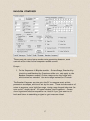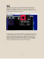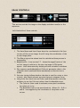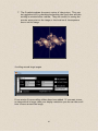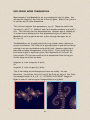
1
FRACTAL SEQUENCER DOCUMENTATION Software Version 3.0 Documentation date 18th December 2013 By Stuart Pryer Fractal Sequencer Web Site http://myweb.tiscali.co.uk/pryer E-Mail [email protected] 1 Looking into the infinite! Fractals are infinitely complex objects created by simple equations. The equations contain complex numbers – both real and imaginary. Fractals contain no straight edges or curves which can be differentiated. They have the property of self similarity. That is similar patterns occur at different scales. If you zoom into a fractal set you will never reach an end. Detail continues forever. Our limitation in creating them is the finite precision of variables held in a computer’s memory. In the natural world there are fractal like objects like fern leaves, branching trees, snowflakes. But you cannot zoom in forever as you will reach the atomic and quantum world. At the plank length – length has no meaning. This software enables you to explore the world of Fractals both as images and as musical sequences. The latter can drive via Midi both virtual synths VST’s and real midi instruments. Have fun. The more you experiment the more you will discover. Stuart Pryer Cornwall 2 CONTENTS VERSION 1 ................................................................................................................... 5 START UP AND WORKFLOW .............................................................................. 5 QUICK START ............................................................................................................. 6 THE FRACTAL SEQUENCER ................................................................................ 7 MIDI ROUTING ....................................................................................................... 9 SETTING UP MIDI IN/OUT for THE SOFTWARE ............................................. 10 USING WITH VIRTUAL INSTRUMENTS .......................................................... 11 EXITING THE SOFTWARE .................................................................................. 11 INTRODUCTION TO THE FRACTAL SEQUENCER ............................................ 12 LOADING, SETTING UP AND RUNNING ......................................................... 12 PC MIDI OUTPUT PORT....................................................................................... 13 FRACTAL SEQUENCER ........................................................................................... 14 THE MANDELBROT SET ..................................................................................... 15 RECORDING SEQUENCES ON SOFTWARE SUCH AS CAKEWALK SONAR, CUBASE ETC. ........................................................................................................ 17 FRACTAL AND RANDOM COMPOSER FORM ................................................ 18 PLAY NOTES ......................................................................................................... 18 STOPPING PROCESS AND NOTES .................................................................... 19 FRACTAL SEQUENCER ....................................................................................... 21 SAVING AND LOADING SEQUENCE PARAMETERS .................................... 22 THE FRACTAL SEQUENCER SETTINGS .............................................................. 24 IMAGINARY NUMBERS AND THE SQUARE ROOT OF -1! ........................... 26 IMAGES .................................................................................................................. 28 JULIA SET .............................................................................................................. 29 SCALES ................................................................................................................... 31 ETHNIC SCALES ................................................................................................... 32 GRAPH & EVOLUTION GRAPH SERIES ........................................................... 33 EVOLUTION PARAMETERS ............................................................................... 34 ARRANGER............................................................................................................ 35 RANDOM COMPOSER ......................................................................................... 37 DRAW ......................................................................................................................... 39 DRAW CONTROLS ............................................................................................... 40 SELECTING A REGION ........................................................................................ 44 EXPLORING MORE DIMENSIONS ..................................................................... 45 PREVIEW FORM ................................................................................................... 47 PREVIEW WINDOW ............................................................................................. 47 IMAGE PROCESSING ROUTINE LOGIC ........................................................... 50 SAVING IMAGES .................................................................................................. 51 IMAGE PROCESSING – I.P. LINEAR OPERATORS ......................................... 52 IMAGE PROCESSING – I.P. NON LINEAR OPERATORS ............................... 55 TOPOGRAPHIC OPERATOR ............................................................................... 55 RANK ORDER OPERATOR.................................................................................. 57 OTHER IMAGING EFFECTS AND FILTERS ..................................................... 58 COLOURISE RGB .................................................................................................. 59 COLOURISE HSL................................................................................................... 61 ANALYSIS .............................................................................................................. 62 ESCAPE TIME MAPPING ..................................................................................... 62 ORBIT MAPPING................................................................................................... 64 3 ANIMATIONS ........................................................................................................ 66 VERSION 2 ................................................................................................................ 67 MUSICAL SEQUENCE ANALYSIS ..................................................................... 67 FINDING SEQUENCES ......................................................................................... 76 COMPOSING .......................................................................................................... 80 MANUAL INPUT OF RHYTHM ........................................................................... 81 FINDING THE JULIA SET FOR A POINT ON THE MANDELBROT SET ...... 83 VERSION 3 ................................................................................................................ 86 RECORDING MIDI IN / MIDI THROUGH .......................................................... 86 PLAYING, RECORDING AND EDITING TYPE 0 AN 1 MIDI FILES .............. 88 BLUE SYNTH 2 - PHASE MODULATED SYNTHESIZER................................ 91 SCALES OTHER THAN C.................................................................................... 94 TRIANGLE INEQUALITY (TIA), STRIPE AND CURVATURE AVERAGE WITH SMOOTH IMAGE COUNT ........................................................................ 95 HISTOGRAM .......................................................................................................... 99 CUMULATIVE HISTOGRAM ............................................................................ 101 LINEAR EQUALISATION .................................................................................. 102 OPEN IMAGE ....................................................................................................... 104 PIXEL CORRECTION FOR NON SQUARE PIXELS ........................................ 104 ZOOM .................................................................................................................... 105 TUTORIAL 1 – IMPROVISING AROUND A USERS MELODY ......................... 107 TUTORIAL 2 - TIPS FOR COMPOSING ................................................................ 110 TUTORIAL 3 - THE CONTROLS & THE SEQUENCER ENGINES .................... 111 TUTORIAL 4 – DRAWING FRACTALS ................................................................ 112 TUTORIAL 5 - DRAWING TIPS ............................................................................. 116 FINALLY .................................................................................................................. 118 REVISION HISTORY – Version numbers ........................................................... 118 CUSTOMER COMMENTS .................................................................................. 122 SO THAT’S IT? ..................................................................................................... 123 CONDITIONS OF USE ........................................................................................ 123 LINKS TO SOME OTHER SITES ....................................................................... 124 RECOMMENDED BOOKS.................................................................................. 124 BACKCOVER ........................................................................................................... 125 NB. Please read conditions of use. Thanks to all of the testers 4 VERSION 1 See Version 2 and 3 sections later for additional features. START UP AND WORKFLOW If you just want to create stunning images then go to the Draw Section. 1. 2. 3. 4. Click the big ‘Draw icon’ on the main form. Click the ’Draw’ button. To draw the Mandelbrot set. Zoom in by selecting a region using you left mouse button Click ‘Redraw’ OR If you want to create musical sequences then set the midi output device using the big ‘Midi’ icon on the main form and then you can approach it from either:- The Composer Module – This contains most of the control settings. Just click ‘Generate’. For default sequence. Or The Draw Module and Composer Module. The Draw module is fascinating as you can explore the images and then from the image create musical sequences which are processed by the Composer module. It also has tools to help find sequences. Check the ‘Play’ checkbox on the Draw Form and Click on the image. Click again on the image for another sequence. 5 QUICK START NB. The demo version 1.7 of this software limits Fractal image size to 256 pixels square and a maximum sequence length of 16 notes. It is also an earlier version with fewer features. The software is designed to assist with musical composition. That is suggest melodies! The more you experiment it the more you will discover its richness. It is an improvement on the module in the Korg Oasys Companion and Triton Controller and works with just about any midi enabled virtual synthesizer or hardware synth. Get ready to explore the infinite! 1. The PC must be running Windows 95/98, ME, NT4, Windows 2000, Windows XP ,Windows Vista ,7, 8,8.1 please check you have drivers loaded for any midi devices etc. – NB. To install it is best to log on with administrator rights and run installation and program as an administrator. It has been written in Microsoft Visual Basic 6 professional SP6. It is a 32 bit application but should run on 64 bit systems. The program is designed for a minimum screen resolution of 1024x600 – use a higher resolution if possible (NB. Also set small fonts - in windows display properties - advanced). Image processing and sequence creation is processor and memory intensive. But the software runs on my netbook. 2. Run the fractal.exe file with administrator rights otherwise windows will not give you the rights to save zoom sequence images you create to the installation directory. To do this right click on Fractal.exe, choose properties. Then select compatibility tab and at the bottom check ‘run this program as an administrator’ Let me know how you get on please ) 6 THE FRACTAL SEQUENCER The main screen contains six menu buttons. See Version 3 for additional buttons. 1. The Red Midi Button allows the user to set up the midi input/output port for the software. This is only used after the software is installed or if the user wants to change the midi routing. 2. The composer button accesses the main control screen for the sequencer. 3. The Preview window allows image processing functions to be performed and the image to be saved as a 24 bit bitmap. 4. The Draw button opens the Fractal Imaging section where the user can draw amazing images of the Mandelbrot and Julia sets. This is a brand new feature from version 1.7 5. The Help button accesses the fractal.pdf help file. This is installed automatically with the software. Updates can be downloaded from my website and the file can be overwritten. 7 Please keep the name the same. ‘Fractal.pdf’. Many controls have tooltips. Just hover the cursor over the control and the tool tip appears. See below. 6. The about button contains my email address and website details. The PC Midi port window allows the user to switch the applications midi output port on and off. 8 MIDI ROUTING This software generates midi note data for sending to midi instruments and version 3 can receive midi in. If you want to get up and running quickly and prefer to read the detailed instruction later, then this is what you need to do:1. Either - Connect the Midi Keyboard to the PC (midi ports or usb) using leads supplied (midi out on the PC to midi in on the synth and midi in on the PC to midi out on the synth or use usb). I use an external midi interface from the M-Audio Midisport range - a midisport 4x4 - which is excellent. Make sure any usb driver is installed. 2. Alternatively use virtual instruments and a virtual midi routing application like midi yoke or loopbe1 to connect see later. 3. Load a sound on the instrument. 4. Set midi channel to 1 on the instrument. 9 SETTING UP MIDI IN/OUT FOR THE SOFTWARE Click ‘Midi Set’ Button (Red midi symbol main toolbar). An example of the midi device list is shown below. Your list will look different. 1. Select midi input/output device connected to the Midi Keyboard or midi routing application for virtual instruments– see later. Do not select the same midi input and output otherwise you will get a midi loop! This may crash the application-depends on midi drivers behaviour. 2. Set midi channel to correct channel – default on this software is 1 (so you can leave it at that), Global midi channel. 3. If you use a German or Austrian PC keyboard check the box that says – German PC Keyboard. This makes playing the Midi software or device from the PC keyboard logical. Note. Z and Y are transposed from US/UK keyboards. 4. Press ‘Apply’ 5. NB. These settings are automatically retained after you close the program in the settings.dat file in the installation directory. 10 Note. To check all is working, if you play a note on the virtual keyboard of the software (composer tab) the instrument should sound. Or Click on the Mandelbrot image to generate your first sequence. USING WITH VIRTUAL INSTRUMENTS If you want to connect the software to a virtual instrument you will need to route the midi signal internally in the PC. There is an easy way to do this. 1. Download the Freeware applications – Either Midi Yoke or LoopBe1. For internal PC midi routing I recommend Midi Yoke http://www.midiox.com/or LoopBe1 http://www.nerds.de which is also excellent. Install either application. 2. Set the Midi output of the Fractal Sequencer to LoopBe1 (internal midi) or Midi Yoke – port 1. 3. Set your DAW (sequencer/recording software) midi input to LoopBe1 (internal midi) or Midi Yoke – port 1 4. You can now transfer midi between the applications! Please note Windows only allows only allows a limited number of midi devices – depends on version. So although you can add more drivers – windows itself will not be able to access them for use! This is a windows limitation and not well documented. Be careful Midi Yoke can use up to 8 slots alone! Normally 4 ports are sufficient. EXITING THE SOFTWARE To Exit the program click on ‘File, Exit’ drop down menu at the top left when the composer form is loaded. The software will close the midi port and sequencer engine will be closed as well. 11 INTRODUCTION TO THE FRACTAL SEQUENCER The Software is a powerful fractal sequencer which can compose music which sounds amazingly similar to human composition. A great way to inspire new compositions! LOADING, SETTING UP AND RUNNING To load the program, 1. Purchase the software – it will be e-mailed to you by return. This contains the software installer and documentation and is around 3mb in size. 2. Install the latest demo version on my website – important! 3. Extract the entire contents to a temporary directory 4. Run the setup.exe file. The settings.dat file and this pdf help file will automatically be installed into your installation directory. 5. Overwrite the Fractal.exe and fractal pdf files with the full version files. Fractal.pdf from my website = documentation. NB. Software updates will normally consist of just an updated .exe file around 1mb in size. The latest help file fractal.pdf can be found on my website. Updated software and help file need to be placed into installation directory. Overwrite or rename old versions. Your PC should be located adjacent to the keyboard. Ideally with the keyboard of the PC at right angles or above the keyboard. As the software is mainly mouse driven all you really need near the keyboard is a screen and mouse. Connect the two devices using midi cables/usb between the PC’s midi port/usb port and the keyboard. USB hubs are not recommended. Turn on the PC, turn on the keyboard and run the program. The first time you run the program, configure the midi device by using the Red ‘Midi Settings’ button main toolbar – top of the display. Then set the midi channel the keyboard (I normally use 1 – this is the default value). The information above will be saved in a settings file at close settings.dat. Please contact me if you have any problems. NB. A few third party midi controllers were not written with fully compliant windows midi drivers. 12 Please read conditions of use. Note… As the program develops, other features will be added. I encourage users to give me feedback and I will endeavour to add new features if requested. PC MIDI OUTPUT PORT The small form which appears when the program is launched opens or closes the PC midi output port. So if you want to launch another program which needs to ‘grab’ the port you must firstly close the port in this application. When you want to use the program again, turn off the other application and just turn the port on again by clicking the radio button – Midi Port On. If you have any midi transmitting problems try turning the port Off and then On again. If this fails restart the software. If that also fails reboot the PC. Important * This pdf help file fractal.pdf will be copied to the same folder as the software’s exe file. Normally C:\program files\fractal..\ do not change its name. NB. It wont work if you name them ‘something else’ or placed in another folder. You will then be able to access them from the program ‘Help’ Buttons which will automatically open your pdf reader and then open the file. Also the context sensitive help will work. Tool bar tips also appear form some commands, 13 FRACTAL SEQUENCER The programme has two main components. The Draw Form and the Fractal and Random composer form. The Draw form enables the user to produce marvellous images of the Mandelbrot Set and Julia sets. It also sends values to the Fractal and Random composer form. Note the Fractal and Random composer form feature section sends midi note data and will work with any midi instrument including the soundcard on a PC. 14 THE MANDELBROT SET The Mandelbrot Set depicted in a picture. 2i – Imaginary number Y axis vertical -2i -2 0 2 Real number X axis ----- A Stunning representation of the infinitely complex Mandelbrot set – the black area. Numbers refer to periodicity in the primary bulbs discussed in the text below. The set exists in a parametric plane as F0 = 0. Fractals use simple equations to generate incredible complexity. In the natural world, complexity is independent of scale. So if you use a microscope to zoom into say a leaf, the complexity does not diminish with magnification ! There is also self similarity. Patters which repeat at different scales. This is why Fractals lend themselves to music. The Mandelbrot set uses a specific equation, F n+1= (Fn)2 + C. This equation generates a new number based upon a previous number in an iterative process. Both F and C are complex numbers of the form a + ib For certain values of a constant C and ‘seed’ F0, the number sequence will 15 not exceed certain limits and it will oscillate or ‘orbit’ around a value. Thus it is possible to generate a sequence of notes using the output from the generator. The constant value generally needs to be between -2 and + 2 otherwise the sequence will diverge to infinity and so the constant will not form part of the Mandelbrot set. In fact the full Mandelbrot set exists in complex number space and the ‘constant’ values which do not diverge to infinity lie in a complex pattern (the black area in the picture above) within the bounds of a circle +-2 and +-2i where (i is square root of -1, an imaginary number). This is the Mandelbrot Set. NB. The sequencer engine is designed to allow sequences to be generated even if values are chosen outside the Mandelbrot Set. So how does it relate to a musical sequencer? Well consider the infinite non divergent series, output from the iteration Fn+1 =(Fn)2 + C. Where F and C are complex numbers. The series could represent midi note values, note timings and lengths ! Think of each point in the black area as a single sequence. As there are an infinite number of points, there are an infinite number of sequences. As described above, the sequencer does not produce random notes, but notes which are related to their predecessor and so forth using the Mandelbrot equation. This produces sequences which can be very close to human composition. For a given constant value, a given sequence will result. However, as there are an infinite number of constant values there are an infinite number of sequences. Very slight difference will result in different sequences, so -1.900000 will be different to -1.899999 although the difference will not become apparent until several, if not many, notes (iterations) into the sequence. As the program variables are double precision the user will not run out of sequences in a hurry! Trial and error is the best way to get started, try values for constants between -1.9 and +0.2. Going beyond +-2.0 or +- 2i will result in divergent data. The software will trap this. You can easily select values by clicking on the large image of the Mandelbrot set which automatically appears when the Mandelbrot Sequencer is selected. Constraining the note values to scales will result in some interesting melodies, and remember to allow plenty of notes to enable the sequence to develop properly. The Fractal sequencer can generate 100,000 notes; more could be easily added if users want. Cutting it short can often miss some interesting sequences. Similarly constraining note length and note interval can make the music appear more natural. The sequence is saved 16 in an array and the user can choose to play back just a section once the sequence is generated. Once you’ve found something interesting, save the settings and use the synth or another midi sequencer to record the sequence permanently in midi. Some of the most interesting sequences result in series which converge or oscillate between values. A constant of -1.9 will not do this but -1.75 will. For very surreal music do not constrain the sequence at all. Pick a pad sound , sit back and listen.. Constants which result in chaotic sequences can often lead to incredible melodies, but remember they may occur just once in a sequence of 50,000 notes ! Tip…Good speakers will enable the very low frequencies to be heard and felt. Also keep the volume at low levels until you are familiar with the sequencer. Im happy to add features if users want them added. To stop the sequence just press ‘Stop Process’ button. RECORDING SEQUENCES ON SOFTWARE SUCH AS CAKEWALK SONAR, CUBASE ETC. You can record sequences on a midi sequencer/editor on a synth or directly into a midi/audio PC sequencer/editor like Cubase or Cakewalk. To do the latter you can use ‘MidiYoke’ - freeware applications from Midi OX ( www.midiox.com ) or LoopBe1 (www.nerds.de) to enable internal PC routing of midi out from the software, to midi in on the DAW. This will enable you to edit the sequence as desired, Alternatively see the section for saving all settings/arranger as a text file which can be loaded for use later – see Saving and Loading sequences. 17 FRACTAL AND RANDOM COMPOSER FORM This is the main form for controlling how the sequencer works. PLAY NOTES This section of the Fractal and Random composer form allows the user to send MIDI note on/off commands. 18 It also has a nifty virtual keyboard for remotely playing the Midi software or device whilst you edit the sounds on the PC. The keyboard from version 2 has a range of 2 octaves. You can also play chords (chord type set in the Random Composer tab) if you choose chord type and tick the box! Or you can play chords on the PC keyboard. Current note number in the sequence and current midi note 0 – 127 are displayed. STOPPING PROCESS AND NOTES The ‘Stop Process button’ stops the fractal sequencer engine and stops all notes. This is the Panic Button ! ‘All Notes Off‘ uses midi command with that name, but beware not all instruments/software respond to it. So I have added a Force Notes Off check box under the button which switches off all notes individually and rapidly for midi notes 0 to 127 , this is a brute force way of stopping notes in this command. Notes decay as per their release envelope. ‘All Sound Off’ button is useful if you get stuck notes as well. However only some midi devices /software respond to it. Notes stop immediately. The Volume Control and Fluctuation volume (randomise) sliders control the volume of any note created. The randomise of volume / velocity and fluctuation value is output in the small grey text box by the sliders. You can also use these features for the sequencer (in the Random Composer tab). If you want to play the Midi software or device using the PC keyboard – press the ‘Use PC Keyboard’ button near the virtual keyboard just before playing. You must press the ‘PC keyboard’ button every time immediately before you use the PC keyboard to play the Midi software or device. PC Key z = Note C. s = note C#. x = note D. etc. The notes run from z s x d c v g b h n j m. Which map to C, C#, D, D# etc. The same applies to Q 2 W 3 E R 5 T 6 Y 7 U , they are 1 octave higher and map to 19 C2, C#2 etc. The ‘PC Keyboard’ is polyphonic. So you can play chords. By the way the polyphony depends on your PC. My old Pentium 2 - 400mhz could play 4 notes at once. My ancient laptop only two notes at once. Depends on keyboard buffer. The pitch of note Z can be set using the ‘note on’ control button at the top left hand side of the form. This facility to play from the PC keyboard has been added to other forms as well to enable the user to audition sounds whilst editing. This feature is for my mate Mastermalleus! 20 FRACTAL SEQUENCER Click ‘Generate sequence’ button to produce a sequence! The controls are now described in detail. 21 SAVING AND LOADING SEQUENCE PARAMETERS 1. If you click the ‘Save As’ menu item (click on File Menu at top left above large icons), the software’s settings file will appear in the arranger tab window and you can save as a text file all the settings and sequences including rhythm etc. So if you want to permanently save a sequence just use the ‘Save As’ menu item – and save as a text file (txt). 2. Pressing Open will load all of the settings from your text file back to the sequencer and will mark the location of the constants by a slightly bigger circle. This is handy for storage of sequences. So recall a previously saved file. Just go to ‘Open’ menu item to open the file, you saved earlier. It then also appears in the arranger viewer. 3. If you want to annotate a file, just add text after the very last comma in the file viewer. You can add as much text as you like. 4. You can use the Edit menu for Cut, Copy, Paste and Find options to edit your annotations. Find with comma separator searches text files with “,” separating data. Find with space separator searches text files with “ “ separating data. 5. You can print to your default printer any text in the text box in the arranger tab. 6. The Exit option closes the program. Use this rather than closing down the window with the windows ‘X’ top right hand corner of the 22 main window. This is so all notes are stopped and the midi port is closed properly. 23 THE FRACTAL SEQUENCER SETTINGS are shown below. NB. The midi note value generated by the software is constrained between 0 and 127 to prevent Midi errors and are reported in the ‘Current Note’ box. Generating Notes - The ‘Note Constant’ value if kept within the Mandelbrot set (black area) will determine the nature of the sequence about an orbit with a seed F0 = 0 and produce interesting sequences. The user can force the sequence to a note range (by checking the box – Enable note range). This fixes the note range as specified in the Random Composer tab. The default is to just use constants comprising real numbers. The user can also select complex numbers by clicking on the radio buttons ‘Real No. part’ or ‘Imaginary component’. The imaginary constant can be input into the pink box under – complex number for note. Press ‘Generate Fractal Seq.’ to start and play sequence. Press ‘Stop Process’ button at top left to stop. Pressing the replay button once you have stopped the sequence will replay the sequence between the notes input into the two boxes below ‘Replay 24 Seq. from Note No.’ button. If the loop check box is ticked the sequence will repeat until the user presses the ‘Stop…’ button. Click ‘Replay sequence from note number’ plays the sequence you created last. Checking ‘Chords’ in the random composer tab – enables generated notes produce chords. These can be selected by chord boxes on the Random Composer tab as needed. Random chords will alternate between various chord types selected or just check 1 chord. The sliders on the Scales tab controlling ‘chord arpeggio timing’, ‘random chord arpeggio’ and ‘chord shell fuzziness’ are also active. Press ‘Frac Seq tab’ to bring up the window again. Some examples - The effect of the value of the ‘real number only’ constant c with the imaginary number = 0. The user can enter this in the text box Note Constant (pink background). Set radio button to ‘real number only’. C= C= C= C= -0.65 -1.6 -1.75 -1.8 C = -1.85 C = 0.2 Tends to a fixed value chaotic period of 3 chaotic near a 3 cycle – intermittent chaotic tends to a fixed value Note Timings - As stated earlier, this sequencer uses the Mandelbrot equation with an orbit of F0 = 0 to define note timings and lengths as well. The 3 boxes below the ‘Generate Fractal Seq.’ button provide the value of the constant for note number, note on time and note duration. (Keep these between +-2, see some suggested values above) The current note time started and length are shown at the bottom. The 2 boxes below and to the right of the constant boxes enable the user to scale the tempo. Default scale is 1. For instance 2 means that either the note on time or note length derived from the equation is doubled respectively. The check boxes constrain the Fractal generator to the values defined in the 6 boxes above the Random Composer tab – Note value, note on range and note off range. The scale factor can applied to the range value afterwards. For note on time – a factor of > 1 will result in an exponentially increasing note separation. Any value between 0.5 and 1 will gradually reduce the note separation over time. 25 IMAGINARY NUMBERS AND THE SQUARE ROOT OF -1! This implementation also allows the user to specify the imaginary part of the complex number. The frames on the right hand part of the Fractal Sequencer tab. This fully represents the Mandelbrot space. Some suggested constants that produce repetitive sequences are shown below: Real constant Imaginary constant * i Note Constant or Time constant Can represent Notes or Time as well -0.12 -0.5 +0.28 +0.38 -0.62 -0.36 -0.67 +0.39 +0.75 +0.56 +0.54 +0.333 +0.43 +0.62 +0.34 +0.22 Periodicity 3 5 4 5 7 8 9 6 The period means that these constants will result in repetitive values and correspond to the Mandelbrot diagram as these occur at ‘Bulbs’ on the diagram with the same number of ‘antenna’ ! These are numbered on the image above. Picking complex numbers in these primary bulbs will result in the periods described above. The two frames headed complex values allow the imaginary part of the constant to be input. Remember, the constant |c| < 2 otherwise you will definitely get divergent data although the software will sort this out using routines I have implemented! 26 The beauty of an infinitely detailed object. A close up of bulb 7 with an attached antenna comprising 7 radiating extensions – Complex numbers with values in the big black primary bulb to the lower right will yield a periodicity of 7 ! Constant c = -0.62 + 0.43i The user can also force the generated notes to a scale (Check box ‘forces note to scale keyboard’) which makes the melodies very ‘human’. Try experimenting with values and instrument sounds – it is definitely worth the time and effort. What you hear is the audio equivalent of the Mandelbrot set with note value and note timing representing the 2 dimensions of the Mandelbrot plane. The mapping function (top right of form) determines how values generated by the sequencer (Either Mandelbrot or Julia set) are turned into midi notes in the range 0-127. 27 IMAGES Sea Horse Valley Julia Set Fatou dust - Star Cluster Period 8 Antenna Julia Set Swirls 28 JULIA SET The other major set is the set in the dynamical plane where starting values of F0 larger than 0 are used. The Julia Set frame enables the user to specify its use by checking the check boxes – ‘Use Julia Set’. Then both the real (a) and (b) imaginary components of F0 (seed) can be entered in the boxes by the user. Press ‘Generate…’ button to create the Julia Set for the note series or timings and to start the sequence playing. Keep values in the boxes small (generally less than +-2 (i) ) otherwise divergent data will interrupt the series and will be error trapped by the software. Note. Clicking the Julia Set check box in the Mandelbrot picture form, changes Julia Set values instead. You must click this as well to enable the Julia set controls in the form above. The right hand side of the box enables Julia Set series to be produced for note timings as well. All the settings in the Julia Set frame are used in conjunction with the Real and Imaginary constant boxes for note and note timings. The fascinating thing about Julia sets are that if the series of F0 = 0 does not diverge to infinity, the Julia set will consist of a finite number of connected pieces. If the series does diverge to infinity the Julia Set is a Cantor Set – that is the Julia Set comprises a ‘cloud’ on unconnected points. 29 A Julia Set is shown above for c = -0.4 + 0.635i on a period 4 bulb. Notice in this stunning image, the infinite detail that is present in the Julia Set. At each node 4 pieces join! Values of F are real in the horizontal axis and imaginary in the vertical Y axis. Thus F0 needs to have values in the black area to produce non divergent data. F0 = 0.1 + 0.1i would work. A non divergent series (ie. in the black area) will always turn into to a repeating 4 note motif. Try it out, set the constants and set the middle note radio button so you use a complex note expression. Change the note range to 0 to 127 – random composer form. The Mapping box allows the user to switch between mapping notes produced by the sequencer by a linear or log function to midi notes in the range 0-127. 30 SCALES This tab defines random, scale based and fractal based compositions. It also has the facility for the user to enter user based scales and a wide selection of standard scales. The Scale based compositions can be further defined by chord arpeggio scales or ethnic scales (see form below) . When you select an arpeggio, the appropriate notes played are determined by the arpeggio scale. So the Arpeggio box allows the user to also play random notes/chords to a scale based arpeggio. You can also input or edit scales on the simplified keyboard in this part of the form which determines how the sequence is constrained. The timing fuzziness control changes the precision, which the arpeggio sounds. The chord shells fuzziness varies the size of the shell (number of notes) sounded. The probability of unchecked noted sounding slider varies the strictness of scale observance by the program. 31 ETHNIC SCALES Above is the ethnic scale controller which permits the choice of international scales, 32 GRAPH & EVOLUTION GRAPH SERIES Note Frequency Distribution of Sequence - Some ‘note constant’ values will converge to a single value (note or timing), others will never converge, others will diverge to infinity and are not part of the Mandelbrot set. However you can still use the divergent series to make a sequence! Try it and see! Divergence to infinity will be safely error trapped by the software. You can see how many times a note occurs in a sequence by clicking on the ‘Show Note Distribution Graph’ tab. See example below. So if middle C (midi note 60) occurs 40 times, the bar in the graph will be 40 units high in the Y axis. The vertical grid separation is set at octave intervals. In the example below the maximum note reoccurrence is 6. 33 EVOLUTION PARAMETERS Imagine you have generated a series containing say 1000 notes. How does the note series develop? Does it converge to 1 note, stay chaotic or become periodic? How do the melodic patterns develop with time? By sampling a ‘frame’ every few notes it’s possible to see on a graph how the distribution of notes changes with time. This can be presented in the form of a movie. So graph 1 (frame 1) shows the first 8 notes, graph 2 (frame 2) the next 8 notes and so on… The Evolution parameter box on the same tab allows the user to specify the note number in the sequence the movie starts, the number of notes sampled every frame and the length at which each frame (graph) lasts. Press the ‘Show Evolution Graph’ button to begin once you have generated a sequence. To stop the movie just press ‘Stop All Notes Off’ button at the bottom of the window. You can also move a frame at a time forward and backwards by using the two arrow buttons. You can again specify the ‘start at note’ number and the number of notes sampled. If the ‘Play selection of seq.’ box is checked the note series in that frame will sound. 34 ARRANGER Musical compositions often consist of repeated motifs – short series of notes or phrases. Many tunes are constructed in this manner. The Fractal sequencer produces in 1 sequence many motifs, which are variations created by the iterative nature of fractals. This simple utility enables the short sections selected by the evolution feature to be captured and stitched together. Up to 7 sections can be added. Thus a complete tune can be produced. This allows a melody to be produced by adding together a series of motifs ! To start, open the Fractal sequencer and press the ‘Arranger’ button at the bottom of the Composer window. Generate a sequence. Note. The text box enables you to see the text files you save when saving sequences or settings. It is also filled when you open a sequence. 1. Pick a section you like containing a few notes using the Evolution Parameters facility. These notes are Motif 1 2. Go to arranger frame and press the top capture button. The start and end note will be transferred from the evolution frame to the arranger frame. 3. Pick a second section you like using the Evolution Parameters facility. These notes are Motif 2 4. Go to arranger frame and press the second capture button down. 5. Press – ‘Play Arrangement’ button. The sequence will be played – Motif 1 , then Motif 2. 35 6. Checking the loop box will play it over and over. Press ‘Stop All Notes Off’ button to finish. 7. Copy sequencer to text box transfers the midi notes to the text box – values 0 – 127. Notes are comma separated. 8. A zero 0 in the right hand column of text boxes in the Arranger window will make the arrangement skip to the next non zero row. 36 RANDOM COMPOSER These controls control pure random note generation however, most controls affect the fractal composer module as well. Except:1. In the Sequencer & Rhythm module - Octave Range, Random Key check box and Random Key Fuzziness slider etc. only apply to the Random Composer module, Octave range varies the range with which notes are sounded. Use note range instead for Fractals. The Random Composer section gets the PC to compose music within parameter envelopes, which are set by the user. These include number of notes in sequence, note high/low range, timing range longest/shortest for note on/off, single/chord – 10 types/random chord types etc. Chosen chord types stored after sequence run. Useful if you just want to sit back and listen to something original or get some new ideas! 37 From Version 2.0 every time you press ‘Start’ a brand new seed will be used to generate a unique sequence. To record a sequence: First go to ‘Fractal Composer’ tab and press ‘Generate Fractal Sequence’. This will populate the note timing arrays based upon your note timing choice. Manual entry etc. Then go to Random Composer tab and press Start repeatedly until you find a sequence you like. Go back to Fractal sequencer tab and press ‘Replay sequence from note number’ The Top Right Section of the form allows the user to input sequences. The program can improvise around the sequence. Input is via the virtual keyboard section after pressing the ‘Record Sequence’ button. Note number, time on and time off can be specified. The rhythm is input manually by entering values or from version 2 entered by tapping the space bar. See Section 2. The Tidy button is for making the note off time constant. This makes a smoother rhythm and a less staccato rhythm when manually inputting. Just set the first note off to a value of your choice (seconds) and press ’Tidy’ The Tempo button multiplies the manual rhythm by (value in box beside it)/120 So if you entered 240 it would double the tempo. 38 DRAW This module can produce the most amazingly detailed images of the Mandelbrot and Quadratic Julia sets. It can also be used to select locations in or outside of the sets to create musical sequences. Click on the main toolbar Draw button to access. A sequence will be created based upon the coordinates at the centre of the user’s selection box – see later. So if the play sequence check box is checked this will automatically transfer the parameter values to the sequence engine and starts playing the sequence. Try selecting areas around the boundary of the set. The so called ‘coast line’ for fantastic images! Areas outside the set produce varied sequences. 39 DRAW CONTROLS This section controls the image on the display and data transfer to the sequencer. Left Hand side of Draw controls. 1. The Xmin/Xmax and Ymin/Ymax show the coordinated at the four corners of the screen image. X and Y being the coordinates of the screen/image plane. 2. The Blue progress bar shows how the calculation/draw process is progressing. 3. Magnification - from version 1.7 - shows the magnification of the current image in relation to the start up image at 256 pixels square. Limit determined by double precision variables in windows. 4. Play sequence sends Mandelbrot/Julia set parameter data to the composer which sends midi data immediately a selection box is drawn. 5. Set note timing defines whether the data is used for notes or time or both. Also check relevant set note timing on composer form. 6. Using Julia Set check box and Julia a and ib parameters sets the software to use the Julia set rather than the Mandelbrot set. The Julia set fixes a and ib and uses screen pixel coordinate for values of x0+iy0. The Mandelbrot set is one special sub set. Where F0 = 0+0i. a and ib = are supplied by the coordinate of the pixels on the screen. 40 7. The Crosshairs shows the exact centre of the picture. They can be toggled on/off by checking/unchecking the check box and this setting is retained after redraw. They are useful for seeing the precise zoom point on the image or the location of the sequence source on the image. Scrolling around large images From version 3 two scrolling sliders have been added. If you want to see an image which is larger than your display resolution you can use the scroll bars to move around the image. 41 Right Hand side of Draw controls. 8. The four coordinate boxes x,y,a,ib define the Julia Set complex number parameters sent to the sequencer. The two boxes that are grey define the plane through the Julia set which is mapped to the screen image. For Julia Set Image Plane see ‘exploring more dimensions’ section. The Julia a/ib boxes show the value of the Julia seed constant C. 9. Update adjusts the four screen coordinate boxes on the left hand side of the form to the appropriate values at the current magnification. This is used if you manually enter values of X,Y,a,b. 10. The four arrows allow the user to move around the image plane. Pan set to 10% of field of view at start of session. 11. The magnifier allows the user to zoom in or out of the image. Zoom set to 2 times at start. 12. No. Of Zoom frames automatically redraws the image successively. So if 3 is set the image will refresh 3 times zooming in on each refresh. 13. Save frames automatically saves a bmp image of the zoom sequence. This can be made into a movie using third party software such as windows movie maker, The bmp images are stored in the installation directory as ‘fractalimage1.bmp, ‘fractalimage2.bmp etc. HD button sets resolution to 1080 pixels vertically – HD standard. Run the software with administrator privileges to do this. 14. Draw/Redraw refreshes the image 15. Reset draws the start image of the Mandelbrot set. 16. Undo – undoes the image to the previous one. One step recorded. 17. The iteration slider determines how many iterations are applied to see if the series is divergent. More iterations slow the calculation process but produce a more accurate and detailed result. 17.The Image Size slider allows the user to decide upon the size of the calculated image. Bigger images take longer to render. Images from 256 up to 4096 pixels square can be drawn in version 1.7 42 depending on PC, Processor and memory. I can increase the image size upon request by customers to pretty much anything! 43 SELECTING A REGION Drawing a square box on the picture with the left mouse button – size as per X dimension. If ‘play’ is not ticked the software will redraw the region in the box - once Draw/Redraw is pressed. If ‘play’ is ticked it only sets values for the sequencer which will begin to play. Note Constant and Imaginary Constant are based upon the coordinated at the centre of the box. You can see the x,y,a,ib values in the text boxes. Grey background indicates the screen image is drawn in that plane. Reminder - Check the ‘Set Note Timing’ box if you want to control note separation timings instead of note values. If you check the ‘set note timings’ box it sets the Time between Note Constant and imaginary Constant. Reminder - Clicking the Julia Set check box changes Julia Set values instead. You must also click on Julia Set check box(s) on the Fractal Sequencer Tab – right hand side. 44 EXPLORING MORE DIMENSIONS Most images of the Mandelbrot set are composed in the x/y plane. You will also see images of the Julia set in the x/y plane. What is very rare is to see the sets in other dimensions. The Julia set requires four parameters. x,y,a,b. These are used in the iteration Fn+1 =(Fn)2 + C. Where F and C are complex numbers. x+iy and C = a+ib. The Julia set is a four dimensional set. Another way of thinking of it is that we are dealing with a four dimensional object of which the Mandelbrot set is a special sub set, a slice through the super set at X0 = iy0 =0! The Mandelbrot set is a plan view with x0+iy0=0 and a and b relating to screen coordinates. The Julia set is typically shown in plan with x0 and y0 relating to screen coordinates and a and b fixed. However depicting in plan does not show the splendour of the object. If you could only see your house in plan it would not give a clear impression of its form. So from version 1.72 you can now slice the 4 dimensional Julia Set object. So the image on screen can show X against a. User to specify Y and b. Or X against b. User to specify Y and a. This is like taking slices through your house vertically. You see Elevations. You will see the true form of the Julia set object. See Julia Set example below. X= 0, y=0, a = -0.745429, b=0.113008. Image on Right is zoom of central region. Images shown in x/y plane. 45 Image on left below is x/a covering region of left hand image above. Image on right is same region for x/b. Notice how this four dimensional object looks very strange and difficult to comprehend for us spatially three dimensional beings. x/a x/b Note that mathematically x/a is the same as y/b and x/b the same as y/a. So y/a and y/b are not options required. This symmetry is due to the symmetry between the real and imaginary numbers. Fractals can be defined by a dimensional property. A simple straight line is 1 dimensional. A square is 2 dimensional. However Fractals have non integer values eg. 1.25. Because they are so tortuous they occupy a space between 1 and 2 dimensions – non integer for fractal lines. However from a solid body perspective the quadratic Julia set is still 4 dimensional. 46 PREVIEW FORM This form allows the user to modify how the image is displayed on the screen or saved to file. In the raw gray scale image the brightness of the pixel is related to whether the series diverges or converges. Black is a divergent series. White is a convergent series. For greyscale the software calculates how many iterations are needed for the value of F to reach a certain pre specified value. Convergent = White. Except for note below. Divergent = Black Note. The Mandelbrot set is shown as black, as when it was discovered in 1979 most computers could only print in black or white. So consequently the very first computer generated image showed divergent series as white and convergent as black. The user can change this, but I have stuck to convention for now so black RGB = 0,0,0 is the default setup! The user can change this. White would be RGB = 255,255,255. PREVIEW WINDOW The purpose of this feature is to allow adjustment of the image processing functions on a small image which is much quicker. Resample reduces the number of pixels speeding the process further. 47 The preview image box holds a 256 or 128 pixel square copy of the main window. It enables comparison between before and after processing. The current Image processing options are shown below and are described in detail. 48 Once the user is happy with the result of changing the various controls, then pressing ‘OK’ will update the main image and the image in memory. You can then apply another image process. 49 IMAGE PROCESSING ROUTINE LOGIC 1. When Draw is clicked an image is produced in the Draw form. Choose image size, bailout, iteration limit, and whether you want an iteration plot – default, or average plot and or smoothing. Alternatively load a bitmap image .BMP. 2. Clicking Preview resamples and copies the main mage array to the Preview form array. Check appropriate ‘enable’ check box to apply an image processing option. Or if you want choose escape time or orbit size mapping then set now in Preview. 3. Click OK updates the main image and the image array. 4. Clicking preview again updates the preview array with the new draw image. Check or uncheck appropriate ‘enable’ check boxes. Apply another image processing function in Preview 5. Click OK updates the main image and the image array. 6. Clicking preview again updates the preview array with the new draw image. Apply another image processing function to preview 7. Click OK updates the main image and the image array. 8. Etc. This way you can stack image processing routines and change their order. Important. Work in monochrome. So goto Preview/RGB/Enable colour and uncheck the colour check box if needed. This avoids stacking colour generation every time you draw and preview which will spoil the final image. You can finally check RGB/HSL colour at the end. If you want you can save your draw form image as a bitmap .BMP file 50 SAVING IMAGES For printing and more sophisticated processing it is useful to export the image as a 3 channel bitmap into programs such as Adobe Photoshop or Astronomical image processing programs such as MaximDL or AIP4Win for example. Reset all colour sliders and clicking ‘Redraw’. Unchecking colourise and HSL does this. This will create a raw greyscale image. Then click ‘Save Bitmap’ to save image to disc. The BMP stores RGB channels as 8 bits per channel. This produces a possible 16.8 million colours. 51 IMAGE PROCESSING – I.P. LINEAR OPERATORS The various kernels are linear operators and convolve the image. That means once applied they can be undone with the inverse kernel. The order in which they are applied (if stacking effects) makes no difference to the final processed image. Some examples are shown below: 52 The image below on the left is a part of a Julia Set and is ‘unprocessed’ other than RGB colourise applied. The image on the right has a Bas Relief Kernel applied. The Image above on the left has an embossing kernel applied. The one on the right a user defined (default kernel) sharpening filter. 53 The image above on the left has a Sobel kernel applied. The one on the right a Kirsch kernel. The image above on the left has a Prewitt kernel applied. The one on the right a Gaussian Blur Kernel. You can start to see the variety of effects possible. They can also be stacked. So once you are happy with the preview. Click OK to update the main window. Then preview and process again! 54 IMAGE PROCESSING – I.P. NON LINEAR OPERATORS The various processes are non linear operators. That means once applied they cannot be undone to retrieve the original image. The order in which they are applied makes a difference to the final image. TOPOGRAPHIC OPERATOR This operator maps iteration count to elevation. So a landscape is produced. The monochrome image on the left was produced using the default settings. The one on the right has inverted elevation and is colourised. Low areas are blue and represent basins of attraction. The light areas are areas of repulsion. In the former, series converge with tight orbits. The latter is the opposite leading to diverging series. 55 The user can specify the elevation of the sun, azimuth and the exaggeration of the height range. Low sun elevations produce dramatic results. The sun is coming from the North West in the images above. The default is inverted landscape to make basins of attraction low elevation. Julia sets are great for this operator. The brightness slider varies the solar intensity, 56 RANK ORDER OPERATOR This operator is used to bring out fine detail in the image (high frequency information) whilst keeping the low frequency data relatively unchanged or reducing it. The radius of the kernel can be adjusted from 1 to 10 pixels. The mix works for Additive and Multiplicative. Middle of slider = 50/50. The brightness varies the brightness of the image. The simple Rank Order process is option 1. Additive, mixes option 1 with the original image. Multiplicative is a more sophisticated process again. Blending the two images. 57 OTHER IMAGING EFFECTS AND FILTERS There are many different filters and effects available in third party image processing applications. Just load a saved bitmap into an application of your choice for artistic effect. Ones which I have used are Adobe Photoshop as well as astronomical image processing packages such as Maxim DL and AIP4WIN. Example - Photoshop – Find Edge Filters such as watercolour and ink pen produce interesting artistic images! 58 COLOURISE RGB To adjust image brightness, contrast and colour in the Red, green Blue colour space:Check Enable, set sliders and click Redraw. It allows fine detail to be brought out of the image. Red/Green/Blue - Contrast is defined as Pixelnew = pixelorginal * (C). The factor C here is 1 to 10. Individual colour channels can be modified independently, in RGB colour space. Red/Green/Blue - Balance (Brightness) is defined as Pixelnew = pixelorginal + (B). The factor B here is 0 to 255. Individual colour channels can be modified independently, in RGB colour space. Red/Green/Blue - Invert colours is defined as 59 Pixelnew = 255 - pixeloriginal. Individual colour channels can be modified independently, in RGB colour space. The convergent series colour is determined by the three text boxes. This allows the user to change the colour from black to any other for the convergent series. So Red would be 255,0,0. 60 COLOURISE HSL The other colour space which images can be rendered in is HSL Hue, saturation and Luminance. This space often gives better images then RGB. This space can also be applied to other operators just like RGB. The Hue slider enables the user to change the colour map of the image cycling through the colour space. The Saturation slider if set to 0 renders a monochrome image. Higher values magnify the saturation. A fixed saturation for the whole image can be selected if the check box – constant - is checked next to it. A saturation value can be chosen by the 0 to 239 slider. The Luminance slider changes the overall luminance by adding a constant to the image. A fixed Luminance for the whole image can be selected if the check box – constant - is checked next to it. A Luminance value can be chosen by the 0 to 239 slider. 61 ANALYSIS ESCAPE TIME MAPPING If both Escape Time Mapping and Show Orbit Vector are unchecked the software is in default mode. This is where the pixel illumination is proportional to the value of the fractal function after a user specified number of iterations. If Escape Time Mapping is checked then the image is a map of the number of iterations before the functions value exceeds the ‘bail out’ point where the software assumes the series diverges. Image colouring is 62 shown in steps. High/Low value shows the iteration number range. Click ‘Enable’ to use. The two approaches are related. The smaller number of iterations to reach the bail out point corresponds to a high value of the function after x iterations. Using the cyclic step function mapping you get a much bigger pallet but is slower. Adjust the colour cycling frequency slider to get the desired result. This is how the colours are mapped to the steps chosen by the escape time map iteration step slider. You can combine this with orbit vector mapping, Topographic operator and Colourise. If Topographic operator is checked the Escape time map will change to a topographic map. 63 ORBIT MAPPING Normally the interior of the set is shown as black. However it is possible to map the size of the modulus of the orbits radius vector to a colour. You can do this outside the set as well. The orbit is the distance between start and finish of the orbit. The orbit is how the value of the formula at each iteration moves around its starting point. Large orbits means the values change quite a bit – this will produce more variable musical sequences. You can combine this with escape time mapping, topographic operator and colourise. To display topographic map you will need to check the ‘Enable’ check box on the Topological Operator Form as well. To colourise, use RGB or HSL as you wish, the check box on the appropriate form needs checking as well. 64 Step function maps are shown below. Rather than have a gradual colour change sometimes it is easier to see if the colours change in discrete steps. This process is a bit slower. . You can change the frequency of change of the step map with the slider on the right. You can also mix and match inside and outside mapping using the check boxes. Moving the colour cyclic frequency slider across further produces a higher resolution map breaking the orbit range into smaller intervals. Try moving the slider even further to the right! 65 ANIMATIONS The software can save a series of bmp images, so you can create an animated sequence if you zoom in. To make a zoom sequence movie:1. Decide how long you want the movie to last. You will need 25 frames/sec to get good High Definition HD TV. But you can use lower frame rate if you want. Low frame reates will produce more of a slide show. 2. Select a point by zooming in manually. 3. Zoom out so you can see the whole set. 4. Select No. Of zoom frames & save frames checkbox 5. Decide upon zoom factor. Click the magnifier. This will start the sequence running. The frame number will be displayed as each one is stored. 6. Once you have a sequence – use software such as the Free Microsoft Movie Maker to turn them into a movie. 7. Note. You may have to run this for a few hours as the number of calculations/frames will generally be large. Make sure you have enough disc space. Remember to run the fractal.exe file as an administrator otherwise windows will not give you the rights to save the images to the installation directory. 8. Of course you could add background music – such as the sequence generated by the zoom point! 66 VERSION 2 This section covers the new features in version 2 of the software. MUSICAL SEQUENCE ANALYSIS Using images to find interesting musical sequences! The images can act as a guide to finding rich areas for musical sequences. The main guidelines are: Use Sequence Analysis to help. See form above. Use the graph in the composer module to see the range of notes the sequence produces for the point chosen. Use the Arranger text box to see the individual midi notes when a sequence is selected Choosing points inside convergent sets will result in converging sequences with more repetitious midi notes. Choosing points outside convergent sets will produce more varied sequences with a wider variety of midi note numbers (notes). 67 The further from the convergent set you go the more varied the notes but there is a trade off as the series will diverge quickly and may very occasionally be stopped by the sequencer. Experiment – as much as possible. The most important thing is to listen to the musical sequence! These guidelines are not rules! Sequence Analysis looks at a musical sequence (up to first 100 notes). Generally the more notes sampled the better – however 10 is a good start = default setting. Here is a simple example. A sequence of just 5 midi notes for a single pixel might look like this:41 56 73 40 78. Number of different notes = 5 = green = number of unique midi notes = number of bars on graph Number of repeated notes = 0 = White = number of midi notes which repeat = number of bars on graph with height > 1 Max number of repeats of any note = 1 = yellow = maximum number of how many times a midi note occurs = max height of bar on graph 40 56 56 40 78. Number of different notes = 3 = cyan Number of repeated notes = 2 = magenta Max number of repeats of any note = 2 = magenta 40 56 56 56 78. Number of different notes = 3= cyan Number of repeated notes = 2 = magenta Max number of repeats of any note = 3 = cyan Remember you are trying to find a sequence which is not just one note repeating. However, think of your favourite melodies. They all contain repeating notes. So it’s a balance. An image is built up by analysing every single pixels sequence! You may need to adjust the contrast sliders to see the image with longer sequences as increasing the number of notes will darken the number of repeated notes image. You can see the list of midi note numbers in the arranger tab text box in the composer module after you select a sequence. 68 See the key on the preview form previous page. When musical sequence analysis is checked you can see how colours map to numbers. Applies if all contrast sliders set to 2 = default and smooth slider set to 1. White = 0. Yellow=1, Magenta 2, Cyan 3, red 4, green 5, blue 6, dark yellow 7, dark magenta 8, dark cyan 9, dark red 10, dark green 11, dark blue 12, darker yellow 13, darker magenta 14, darker cyan 15, dark grey 16, Black >=17. However if you move the contrast sliders on the form the key colours will update automatically. The user can vary the colour contrast for RGB individually. 0= colour channel invisible. The number of notes analysed in a sequence can be adjusted from 1 to 100. As this analysis has to do millions of calculations you need to let the computer process for several minutes. Larger values are slower to process. A 256 pixel sq. image on my netbook takes 6 1/2 minutes to render an image for 10 notes. Only 1 minute on my pc. This is where the preview option helps to save time by using smaller/resampled images. Click on play on the draw form and explore. Remember to select the sequence type – real only, real part of complex or imaginary part of complex on composer form as well. NB. The notes are mapped from the fractal series number sequence +-0 to 10126 (i) to midi note numbers 1 to 128, using sophisticated routines controlled by the composer form controls and the sequencer engine. The ‘smooth 1x to 10x’ slider multiplies the note range by a factor of 1 to 10. 1 is normal. 5 means 5 notes now occupy a colour. So magenta = 2 – 3 notes smooth of 1 = default value, is now notes 5 x 2 to 5 x 3 = 10 – 15 notes. This can smooth out a speckled image (which occur in chaotic areas) to make the image clearer. Normally a smoothing value of 2 is sufficient. 69 The image on the left above is the dendrite Julia set fractal. Sampled 10 notes deep. Smooth set to 1. The simpler image on the right is smoothed by 4. White = 0 to 3 notes repeated. Yellow = 4 to 7 notes repeated. Magenta 8 to 10 notes repeated. The image above is a simple quadratic equation of the form X(n+1) = x(n)2 + c. X and C are real numbers only. Number of different notes plotted. Red lines are very thin and have the minimum number of different notes. Green indicates more different notes. Blue indicates even more different notes in sequence etc. Black has most different notes. 70 In the image above bright colours indicate more different notes in the sequence. Map of real number part of complex number equations used as musical sequence. Notice this strange mapping of the Mandelbrot set. A shadow of the source set can be rendered in the background using the Background Image Contrast slider. Note. Imaginary numbers used in the complex number equations for musical sequence produce totally different sequences. Looking 40 notes deep at every pixel into the Mandelbrot set - image above. Brighter colours show more repeated notes. i.e. A less varied sequence. Areas outside the set are richer. To get the corresponding midi sequence, select the appropriate radio button on the composer module before you draw it and after it is drawn, check play sequence and use the draw box to select a sequence. 71 If you draw using imaginary numbers only for sequence, select the Imaginary Component radio button. The image above is of the start up Julia set - number of repeated notes. If you draw using a Julia set checking the ‘Julia set’ on the draw form or change the Julia set drop down list, the software will automatically update the parameters on the composer form. Then click ‘Play Sequence’ check box and select with the mouse a location by drawing a box. Hold down left mouse button and drag the box or just clicking once at a point. The midi notes will then be generated and sent to midi out. 72 Image above. Magnification X10 of a rich seam of sequences in the image above. Red only 4 notes repeated. Green 5 notes repeated, Blue 6 etc. Other image processing features such as kernel etc. can be applied as after clicking OK’ the main image array is updated. So click preview after the main image is redrawn and the image can be manipulated further. Emboss for instance brings out the detail well. Once you are happy with the image, clicking OK again will transfer the image to the main window so you can try different sequences. The image above has been analysed for the number of different notes in sequence. Compare this to the one in the Musical Analysis form window at the start of this section. Processing makes a clearer image – but the colours no longer correspond to the note numbers as HSL is used. An 73 emboss filter has been applied to the original image and then it has been HSL colour coded. Black = few different notes. Yellow = mainly different notes. The low lying areas in black will produce sequences with many repeated notes. Green a few less repetitions. The magenta plateau will be much better. The yellow hills are even better again. The image above is the imaginary cousin of the one previous. This shows maximum number of repeats of any note. An emboss filter has been applied to the original image and then it has been HSL colour coded. A Circle Julia set. An emboss filter has been applied (right hand image) to the original image (left) and then it has been HSL colour coded. 74 Without Musical Sequence Analysis finding sequence rich areas involves much more ‘trial and error’. Remember zooming in will increase the sequence numbers as fractals are infinitely detailed! Also zooming out will uncover areas further outside of the set which will be rich as well! Chaos. The image above is of the start up Julia set – number of different notes. It clearly shows the chaotic nature of the set and its surroundings. Very small movements in the plane result in very different sequences. Rich hunting grounds far outside of the Mandelbrot set. Zoom 0.2 on start image. An emboss filter has been applied (right hand image) to the original image on the left – number of repeated notes - and then it has been HSL colour coded. 75 FINDING SEQUENCES From Version 2.0 there is the option for finding sequences that the user inputs and then letting the software continue the composition. The software develops the sequence using the fractal set parameters from where the user left off! Because fractals exhibit self similarity, not only at different scales across the image but in the iterations for each pixel human like compositions can be created. You could input your favourite melody and hear variations on how it can be extended. Note you may not find some sequences you enter or you may have to do some hunting in the different sets. 1. The first step is to decide what fractal you want to use and draw it on the main form. 2. Then click on the ‘Find Sequence’ radio button on the Musical Sequence Analysis form at the bottom - Version 2.00 default. (see above) 3. Then play a sequence on the virtual piano keyboard on the Composer form. Up to 16 consecutive notes can be saved. These will be displayed on the Random Composer sequencer form. Setting a note to 0, say at note 4 will mean that the software assumes you want no further intervals checked beyond note 3 (2 intervals). 4. Then decide if you want the search on the Preview Image – default setting - or the Draw form image. You can decide by using the radio buttons in Compose Sequence (see next image). The main form allows much larger images giving many more sequences. But the trade off is it takes longer to process. For big images 100 notes deep it could take several hours depending on the PC. A 76 sequence of 2 intervals, 20 notes deep, 128 pixels square will take several seconds on a medium spec PC. 5. Decide on how many notes deep you want to allocate per pixel. “20 is a good starting point. 100 will take longer to process! 6. Either click Preview or OK depending on which image you choose. The resulting image will show how many intervals (= number of notes - 1) are found which match you melody. For instance type in a sequence of 5 notes. There are 4 intervals. Note. For instance the interval between midi note number 65 and 67 is 2. Between 40 and 50 = 10. The analysis is musical key independent. The Software will match these intervals. If you don’t get many matches try another fractal set. For instance the Dendrite fractal is quite different from the Mandelbrot set in this respect. If only 1 matching interval is found nothing will be saved. Ie 2 notes. See image below. White no matches. Yellow 1 interval match. If 2 intervals (3 notes) agree the software will record the sequence parameters. If 3 intervals (4 notes ) agree the software will record the sequence parameters again. Etc. Below 10 intervals /11 notes match = Red. 77 This will be repeated until 15 intervals are checked (or until a 0 is found as a note number in your sequence) for the best match for every pixel. The resulting image will then colour code the matches. White = 0 intervals match, Yellow = 1 intervals match. Magenta = 2 intervals match – sequence parameters stored. Cyan = 3 intervals match – sequence parameters stored. etc. Image Above. Variations on The Blue Danube Waltz. The hidden treasures in the Mandelbrot Set. The big magenta area shows 2 intervals/3 notes match. 29,953 pixels! A smattering of cyan pixels show 3 intervals/4 notes match. 383 pixels. There are 36 matches for 4 intervals/5 notes – see image below. None higher. To get higher ones increase note depth from 20 up to 100. Increase image size using main image window or zoom out or in to regions which have high matches already. 78 Image above shows the ‘Compose Sequence’ controls. 36 matching sequences found for 4 intervals/5 notes. Pressing load next sequence with the ‘play whole sequence’ check box checked will play the whole sequence from note 0. It will send the midi data to your instrument of choice. The image above is the Circle Julia set. Sequence analysed is of 8 identical notes, 20 notes deep. Small red circles are pixels auditioned by the user. The best matching region for a repetitive sequence unsurprisingly is inside of the set where the series converge. You may find you cannot find a matching sequence in the set. You can then use ‘Accept Note Sequence Variance’ check box. What this does is allow for variations on your sequence. If you enter say 65 66 67 as midi note numbers. This will permit a set sequence of say 65 72 66 77. Ie it will allow notes to be inserted between notes in your sequence so a set sequence can be found. Whilst strict sequence compliance is lost you will still get an interesting and similar sequence in most cases. 79 COMPOSING The next step is looking at the results and hearing the alternative sequences the software comes up with. This bit is great fun! 1. Choose how many identical intervals you will accept. You may typically only get up to 10 matching intervals for a 256 pixel square image, analysed for 20 notes/pixel. You can see the results using the up/down button to change the value – say to 3. Then click ‘Find Number of Sequences’ to see how many sequences agree. You may get several hundred. Fewer generally, as you search for more matching intervals per pixel. 2. ‘Load Next Sequence’ will load the first sequence and report where in the sequence the agreement begins as well as the pixels coordinates. NB. 0, 0 is top left. Your sequence may not start until 5 notes in say. A red circle of 5 pixels radius will be drawn around the pixel generating the sequence. 3. Checking ‘Play’ checkbox will automatically start the midi stream to your instrument or VST if ‘Load Next Sequence’ is clicked. 4. To go to the start position where there is a match. Press ‘Stop Process’ on the Composer Form. The press ‘Replay Sequence from Note Number’ on the same form. The start note will be filled in for you automatically. You should then hear your sequence and then what happens next! You may have many sequences to choose from. 80 MANUAL INPUT OF RHYTHM From Version 2.0 the user can tap in the rhythm of the sequence using the computer keyboards space bar. This has been added following the requests of several users. This option is now set by default - Manual Rhythm - as in my experience it generally gives the best results for any sequence. A new option has been added to the Fractal Sequence tab. See below. In the sequencer frame – Random Composer - there is a tempo button and text box so you can vary the tempo after you have recorded your rhythm. There is a simple default rhythm set when you load the software. Default tempo is assumed 120. You can enter tempo at any speed but 120 in the text box will playback as you entered it. 240 will double the tempo. 60 will halve it etc. Pressing ‘Tempo’ also quantises the timings so that each time is rounded. So if the recorded timings were 0.15, 0.132, 0.122. sec Then if the quantise text box is set to 0.1 sec then the timings would be 0.1, 0.1, 0.1 sec It is best to set the quantise box to less than half the smallest time you record to avoid getting a machine like accuracy. To change the default rhythm. Go to Random composer tab. I find it helpful to hear actual notes so checking ‘Play Sequencer Note’ sounds the associated note in the sequencer by sending midi. 81 Check ‘Tap Space bar to Input Rhythm’. You must do this immediately before tapping the rhythm out on the space bar. See below. If you make a mistake press Reset Sequence and then Check ‘Tap Space bar to Input Rhythm’ Now Tap the space bar to record up to 16 beats. Space bar down note on. Up note off. Time Signatures. To use fewer beats – just set the timing boxes ‘ On/Off’ to 0 after your last beat. For instance 4/4 or 2/2 time could use all 16 beats (text boxes) as 16 is divisible by 2 and 4. You could also use 8 or 4 beats only. 3/4 time will use 15 beats as 15 is divisible by 3. You could use 12 or 9 or 6 or 3 beats. See image below with 0’s in last two boxes to reduce sequence to 15 beats. 6/4 time will use 12 beats or 6 beats etc. NB. Note, Octave Range and Random Key fuzziness is not used with the Fractal Sequencer, they are used with the Random Composer. +/- buttons raise all note numbers by +/- 1 semitone at each press. If you use the ‘Save’ option in the menu bar of the composer form the 16 notes and their on/off values will be saved together with all of the fractal parameters etc. 82 FINDING THE JULIA SET FOR A POINT ON THE MANDELBROT SET As discussed earlier. For every point on the Mandelbrot set there is an associated Julia Set. Or, every Julia Set produces a point on the Mandelbrot set with X0, iY0 =0 From version 2.1 you can easily switch between the 2 sets. In the example below, a region at the boundary of the Mandelbrot set is selected with the left mouse button. I want to see what the associated Julia set looks like for the region of the Mandelbrot set displayed above with the small square box. Check the Julia Set check box and select ‘Swap Sets’ from the drop down box. Click Draw/Redraw. The Julia set is shown below with its a, ib constant value set as the coordinate at the centre of the square box you have drawn previously! 83 You can work the other way also. If you have a Julia Set, then by unchecking the Julia set box and selecting ‘Swap Sets’ from the drop down box you can see where on the Mandelbrot set the Julia set lies. Click Redraw. You can use the crosshairs to see the precise point. For the infinite number of points in the Mandelbrot set there are an infinite number of Julia Sets. Try exploring around the boundary of the Mandelbrot bulb. Inside the bulb the Julia sets are connected with olid regions. Outside they are disconnected consisting of discrete points. 84 Above right is a Julia set (Douady’s Rabbit) from a point inside the top bud of the Mandelbrot set top left. It is connected. Below is a Julia set (Dendrite) from a point above the top bud and outside of the Mandelbrot set. It is not connected and if you zoom in enough the individual points would not be in contact. The fun thing is there are an infinite number of Julia sets to explore and draw! See an interesting feature I found below. a=0.3, b=0. 85 VERSION 3 This section covers the new features in version 3 of the software. RECORDING MIDI IN / MIDI THROUGH The Main Menu bar has been added to. The Green Midi Button activates the PC Midi Output Port control. This is activated by default at load. But if you close it you can reopen it with the Green Midi Button. The Yellow Midi Button opens the Midi In control form. This is used to open the midi in port of the software by pressing ‘Receive MIDI Notes/Thru’ Button. This Enables Midi Through for MIDI Messages which go straight to the programs output port. As notes are played The midi message number, data1 and data 2 are listed in the MIDI data box. Latest message at the top. To stop MIDI IN/Through press ‘ STOP MIDI IN. 86 To Record 16 Midi notes and their timings into the programs sequencer check ‘Record 16 Note Sequence’ checkbox. This populates the sequencer in the Composer/Random Composer form. Once note 16 is releases an information box will confirm. Click ok. You can then use the Fractal Sequencer to produce variations on your melody! Note. Play Mono-phonically when recording, with only 1 note sounding at a time. So finish 1 note before starting another. The software has a routine which forces the recording in this feature to monophonic. So if you play a note, you cannot play another note until the first note is released. ie. a note-off message is received for the first note. The Software receives and transmits midi messages in the form message, data 1, data2 or system exclusive messages. You can stop midi through by unchecking ‘Thru’ in the MIDI menu - above the main forms buttons. Sysex messages can be passed through if - ‘SYSEXTHRU’ is checked. This opens up the form as below. Individual messages are listed on the ‘Sysex Message List’ text box. Click on a message to see its contents in Hexadecimal in the box below. There are also 3 midi filters – time clock, undefined and active sensing which can be selected. Normally you will not to change these – so leave them checked. You can input midi data from a midi controller, midi enabled keyboard etc. or midi player! 87 PLAYING, RECORDING AND EDITING TYPE 0 AN 1 MIDI FILES A free dedicated stand alone midi file player is now available. Place the Midiplayer.exe file in the fractal sequencer installation directory. Click on the ‘Midi Play Rec’ button on the fractal sequencer main form to open it from within the software. NB. Careful as clicking twice will open another instance. It can create, edit and play type 0 – single track and type 1 multi-track midi files. This is dedicated to the Fractal sequencer software although you can use it independently, and is useful if you don’t want to use a full blown DAW (Digital Audio Workstation) software. To Play a midi file:1. Choose your midi input and output in the drop down boxes. Avoid midi feedback by not having the same input and output device 2. Make sure you have a suitable instrument attached to the output port. 3. Select ‘File / Open’ and browse to a midi type 0 or 1 file. 4. Click on the track you want in the ‘ Tracks box’ 5. Press ‘Prepare to Play Current Track’ 6. Press Play then Stop when finished You can also Play a monophonic track into the Fractal Sequencer Midi In and record up to a 16 note sequence for analysis and get the software to 88 produce variations. Set the Midi out port of the Midi File Player to the Input Port of the Fractal sequencer. Just be careful to avoid midi feedback by not having loops. Ie. Input Midi file player port 3 output port 1 to - Fractal sequencer input port 1, Output port Fractal sequencer port 2, to a suitable instrument. To Record a midi file:1. Choose your midi input and output in the drop down boxes. Avoid midi feedback by not having the same input and output device 2. Select the output of a midi instrument or the fractal sequencer 3. Select ‘File / New’. 4. Press ‘Record’ then Press Stop when finished 5. Select File / Save As and name file - a midi type 0 or 1 file name – browse to the save location. To Edit a midi file:Click on File/Edit. This will widen the form to show the editor controls. 1. Open a midi file 2. Select track to edit – left text box 3. Click on the message box- right box - on the line you wish to edit – this will fill the editor controls with the parameters of theat message which you can edit. 4. Change parameter(s) in the editor text boxes 5. Press Modify button or Insert a recording – check box 89 6. When you have finished – save file If you want to insert data just press ‘Insert’ and enter the data in the editor. To delete data press ’Delete’. You can use Hex or decimal data – just uncheck the check box for decimal. 90 BLUE SYNTH 2 - PHASE MODULATED SYNTHESIZER A free dedicated stand alone synth is now available. Place the blue2.exe file in the fractal sequencer installation directory. Click on the ‘Blue Synth’ button on the fractal sequencer main form to open it from within the software. NB. Careful as clicking twice will open another instance. The Blue Synth is a free two oscillator phase modulation virtual synthesizer designed to provide a useful audio source for the Fractal Sequencer. Its can produce lush pads or powerful leads. It is available as a standalone application for running with the Fractal Sequencer. Place the blue2.exe file in the Fractal Sequencer installation directory. There are two oscillators to create the carrier waves which can both be phase modulated by a sine wave. The polyphony can be adjusted between 1 and 128 notes. You can choose the carrier waveform and apply an attack, decay, sustain and release envelope whose amount can be adjusted. The Freq PM knobs control the phase modulation frequency, 0 is no modulation 1 is full modulation at half sampling rate. Oscillator 2 can be detuned. The output can be fed through two filter banks with cutoff, resonance and track as well as ADSRs’ affecting the filters. Programs can be saved. 91 There are 10 factory sounds preloaded in the synth courtesy of Yoa out of the 20 available program slots in each program bank. Programs/banks can be saved as text files. Please set midi and audio preferences ( direct sound or ASIO) in standalone version first. Nb. When playing into the fractal sequencer’s inbuilt 16 note sequencer set to monophonic = 1 voice. The download is free. All I ask is for feedback and ideas for additions or modifications. Also additional programs/banks welcome. I will host on my site. website. http://myweb.tiscali.co.uk/pryer/ PC Specs. Windows XP , 7,8 or 8.1 - Laptop or PC - ideally >2gb ram and >2ghz processor. Should run on a netbook depending on specs. Main features 1. Click on red LED to clear audio – panic button 2. Oscillator 1 and 2 have a choice of waveforms. Sine, square, Sawtooth, triangle and noise. 1 to 128 note polyphony. 3. Osc 2 Pitch – adjust by up to +- 5 octaves, semitone and fine. Slightly detuning richens sound. 4. 2 Envelopes per oscillator control volume and cut-off frequency 5. Filter – cut-off and resonance – filter type selectable. Polyphony 1 to 128 notes. 6. 88 note on-screen keyboard activated by mouse or use PC keyboard keys or even better your own external midi keyboard. Full 128 midi notes accessible. 7. A stereo ping pong delay enriches the sound. 8. See fractal sequencer/composer which can be used with synth and midi yoke or loopbe1 freeware to connect. Program/bank load and save. 9. There are 20 factory sounds preloaded in the synth courtesy of Yoa (see link below) out of the 40 available program slots in each program bank. Programs/banks can be saved/loaded as text files. 92 10. In standalone set midi in & midi out/audio/zoom feature at top of window. For more information email me at [email protected] Copyright Stuart Pryer – November 2013 Special thanks to Yoa, who helped with creating the presets and demo songs, as well as beta testing. https://www.facebook.com/pages/Yoa/225581710813417 . Soundcloud (http://soundcloud.com/yoa01) and blog (http://siryoa.blogspot.com/). 93 SCALES OTHER THAN C A new feature has been added to the scale keyboard. If you check ‘ Force Note to Scale’ on the Fractal Sequencer you can control the scale of the resulting sequence. Below is the scale C minor. To get C minor (C is default scale) press the Ethnic Scale button and select the scale in the ethnic scale form. If you want C# minor you could do that by transposing each check to the right by one note. The new way is to click the ‘+1 Semitone’ button. Click again for D minor etc. The number of semitones from the start position is reported in the text box – this shows as 0 in the above image for C minor. There is also a ‘-1 Semitone’ button. 94 TRIANGLE INEQUALITY (TIA), STRIPE AND CURVATURE AVERAGE WITH SMOOTH IMAGE COUNT Note. From version 3 the default mode for images is monochrome. The colourising is done at the end of image processing. This is because it is important not to stack colourisation as version 3 allows for repeated processes. Ie. Draw then Preview, image process, OK, Preview,image process, OK etc. So you could do a Rank Order convolution and press OK. Then Preview and do a topographic convolution on it etc. You can of course preview colour at any stage just turn enable colour off before you do another process. The TIA process often makes the image more pleasing by reducing image contrast and smoothing the image but it increases the image generation time. It looks at how the orbit for each pixel moves in relation to its upper and lower bound using 3 different approaches and smoothes the iteration steps in the output image. From Version 3 you can adjust the bailout value. This is the value which determines when the calculation iterations stop. It can be varied between 3+ (10^0) =4 and 10^22! For normal fractal images the number of iterations determines the detail inside the convergent set. Outside the set, the bailout point determines the detail but you have to allow enough iterations to reach the bailout point. Normally >500 iterations and a bailout value of 10^8 is sufficient for a reasonable image using this approach. Move the two sliders a bit to the right to improve the image. 95 For TIA, 1000 iterations and a bailout value of 10^22 will produce good images but they may take minutes or hours to produce depending on image resolutions and your PC specifications. So start off with a 256 pixel square image. When you have set the sliders to a good setting you can then increase the image size. Smoothing without TIA will require less iterations and a lower bailout. Choose ‘Average’ check box by the Draw button, This accesses TIA , Stripe and Curvature average. You can adjust the range of iterations (terms of the series) for which the process analyses the image (upper & lower bounds iteration %), change the bailout value and select smooth Iteration Count. Increase the Iterations from 100 to 1000/2000 for cleaner results! If you use analysis tools such as Rank order, Topographic and Kernel operators adjust the contrast and brightness sliders as the original TIA image is lower contrast. Below left. Normal iteration count/bailout image, Below right. Smooth iteration Count and Averages compared using similar HSL settings for Lyra Julia set. Original Image Original Image HSL Colour Coded You can use Smooth Iteration Count without Average and this will smooth the final image. 96 Smooth Iteration Count HSL TIA without Smoothing HSL TIA Smooth Iteration Count Stripe Av. + Smooth Iteration Count Stripe average uses a trigonometric function for the terms of the sum rather than ratios and produces radially striped images. The slider changes the stripe frequency 1 to 50. See two images with same hsl settings. 97 Curvature Average looks at how the curvature of the iteration function changes. See Above image with HSL coding. From version 3 the colour sliders in Preview-colour can be set to between -255 and 255 so that bright images can be made darker as TIA will naturally produce brighter images. Just move the sliders to the left to darken an image. 98 HISTOGRAM The histogram check box in Preview opens the pixel brightness histogram window. This is used to fine tune the output image to avoid over or under exposing your image. Ideally all image pixels in the red,green,blue channels should fall in the brightness range 0 to 255. Typically there should be no ‘bars’ higher than 1 at 0 or 255 brightness levels but it depends on personal preference. Most pixels should fall in the range 0 to 255 – see below. Each bar represents how many pixels (y axis) at each brightness level 0 to 255 (x axis) for the three colour channels. In addition to the various contrast and brightness controls in the image processing functions there are Transfer Functions – for modifying the pixel distribution. Select option and click Preview. Original - Default a x Log(x) Square Root Squared Gamma – cut / boost midrange GammaLog – cut / boost midrange Y=aX Y=-aX Y=Sin(aX) 99 The log and the last 5 options have a slider for further modification by a factor ‘a’. Remember that if you stack more than a couple of image processing routines then uncheck ‘enable colour’ ie. monochrome before redrawing or doing another Preview to stop the image array being affected by re applying colourisation multiple times. Uncheck - Preview/Colour/RGB 0r HSL/Enable Colour. Final colourisation is normally done at the end before saving or printing. See close up of previous images below. This is the Lyra Julia set. Stripe average and smooth iteration count. 500 iterations with a bailout set to 10^6. Stripe frequency 11. On the previous image notice the colour histogram. The bright pixels in the monochrome image (left) are mapped to the blue channel. The mid brightness pixels are mapped to green and the low brightness pixels to red. See the right hand image. This has been done by just using the RGB contrast and brightness colour sliders. Moving a contrast slider to the right spreads the pixel values for that channel. Moving a brightness slider to the right moves the entire set of channel pixels to the right. The final colourised image is on the right. These are jpeg images in this document. The original bitmap is even more detailed. From version 3 the RGB contrast sliders range no go from 0.1 to 10 (1 to 100 slider values). 100 CUMULATIVE HISTOGRAM Check the ‘Cumulative Histogram’ check box. The software can display a cumulative histogram . Imagine a histogram with a series 2,5,7. If the terms are added successively you get 2,7,14. So it’s a running sum. See image above. 0 pixels are present at value 0 brightness. 100% of pixels are less bright than the maximum value of the graph. 101 LINEAR EQUALISATION See the check box ‘Linear Equalisation below the four arrow buttons. This process re distributes the pixel values to make a more dynamic image. Check box and click ‘Draw’. An unequalised image will be produced after which the histogram is then equalised. Click ‘Preview’ to see it. If you are happy with the result then click OK to produce the image on the main form. The box will uncheck after process completes. This process adds a few seconds to the processing time depending on image size. See cumulative histogram below and compare it to the one without equalisation in the cumulative histogram section earlier. The original curved histogram is straightened. 102 Compare the two images below. The left hand one is without linear equalisation. The right one is with equalisation. In the right hand image there are equal number of pixels at each brightness level 0 to 255 – see histogram above. This produces more contrast or ‘punch’ in the image. No equalisation Linear Equalisation Lyra Julia set. Bailout 10^22 with 2000 iterations. Smooth iteration count. Stripe average with frequency 8. Start up Julia Set. Bailout 10^7, 1200 iterations. Linear Equalisation HSL colour coded. 103 OPEN IMAGE You can open previously saved 24bit bitmaps. Go to Preview/File/Open. The main Draw form picture will be replaced with the opened image in monochrome. Remember to work in monochrome and finally colourise. NB. To reload musical sequences you have to go to Load sequence settings and reload the setting file. See Saving and Loading sequence parameters. PIXEL CORRECTION FOR NON SQUARE PIXELS In Preview/Analysis/Compose Sequence a text box has been added to allow correction of non square pixels. Most PC monitors have pixels which are not square. On my PC’s the ratio of heighy/width varies between 1.333 qand 1.425. This box allows you to enter a value appropriate to your PC/Monitor. The value is saved at close in the settings.dat file and reloaded automatically at launch. To adjust try a value – say 1.4. Save a bitmap. Then reload it. If there are grey areas at the bottom of the reloaded image the factor needs increasing. If the picture is cut off at the bottom then reduce it. You may need a different factor for each PC. 104 ZOOM Sometimes it’s useful to be able to zoom into the main image to seek out interesting areas rather than Re-drawing. Click on zoom and a zoom window opens – right hand image below. Also, a square box appears on the main image – left hand size. Click inside the box to move it around and a zoomed image appears instantly in the zoom window. The slider below the Zoom window varies the box size in pixels - 30 to 200. The Zoom factor varies inversely with the box size. (x8 to x1.25). The picture below left is a magnified view of the centre of the left hand image above. The right hand image is magnified 300x at point 0,0. Emboss and HSL colour coded. Does the detail continue further? 105 Yes. And as far as we know it continues further and further, forever! Magnification 1800x. TIA, Smoothing, Equalisation. HSL colour coded. Start up Julia set around x=iy=0. 106 TUTORIAL 1 – IMPROVISING AROUND A USERS MELODY This Tutorial describes how to get the software to develop a melody around one a user has composed or one the user likes. 1. Load the software. Click on the Composer menu button at the top of the screen. Then click on the Random Composer tab. 2. Connect your instrument or VST of choice. Then play the virtual keyboard and enter up to 16 notes. Timing is not important at this stage. After the last note, if you don’t require all 16 just enter 0s’ in the boxes in the sequencer module. 3. Now enter the Rhythm manually by checking both boxes – Tap Space bar to input Rhythm + Play Sequencer Note. You will hear the notes played as you tap the space bar. Enter 0s’ in any unused timing boxes – as below after midi note 71. From Version 3 you can enter the notes/timings from your MIDI keyboard/controller as well. 107 4. You have now stored the rhythm and melody. Click on the Fractal Sequencer tab. ‘Use Manual Rhythm’ radio button will be set as default for you already. 5. Click on the Draw Button menu button at the top of the screen. Click ‘Draw’. The Mandelbrot set will appear after a short time – a second or two depending on your PC specification. 6. Click on the ‘Preview’ menu button at the top of the screen. Then select Analysis from the menu bar – and musical sequence analysis. Check the ‘Allow Note Sequence Variance’ and ‘Enable’ check boxes. Set the ‘Number of Notes sampled slider’ to 100. Set the image to 128 pixels and resample to 3x3. Click Preview. 7. After a minute or two a small 128 pixel square Image will appear. This is the image representing how the software has matched your melody with ones ‘hidden’ in the Fractal set. 8. Now select from the menu at the top of the Preview Form – Analysis – Compose Sequence. Here you can decide on how many matching intervals you will accept. Select a number with the up/down arrows. Say 4. Click ‘Find Number of Sequences Found’. Then Check ‘Play Whole Sequence Automatically’ and finally press – Load Next Sequence. You First melody variation will play on your instrument. 108 1. . If you don’t like it press Load Next Sequence again for another version etc. You can also explore larger or smaller identical intervals. 109 TUTORIAL 2 - TIPS FOR COMPOSING Once you have found a sequence you like you can use many of the features in the composer section to refine it: 1. Listen carefully as it’s all about music! 2. Use ‘Accept Note Sequence Variance’ check box if you cannot find a perfect match for your sequence 3. Check note distribution in the Graph tab and midi note list in the arranger tab. 4. In the Random Composer section Change the note range – say 2 octaves by specifying min and max midi note numbers, timing range and your choice of chord types. 5. Manual input of tempo is normally the best way of giving the sequence its rhythm. 6. On the Fractal Sequencer form. Check ‘ Force Notes to Scale Keyboard’ 7. On the Scales tab – click Ethnic Scales’ button and select a suitable scale. For orchestral music you might want to use predominately minor scales. For Rock music it may be a mixture of major and minor. For traditional or folk music you will probably use major scales. For jazz probably pentatonic scales etc. You can input your own by checking the Scale Keyboard check boxes. Also select a suitable Arpeggio Type. Check Random Chord shells and Random Arpeggio. 8. Use chords when ‘Replay’ is clicked on the Fractal Sequencer tab 9. As an option - Arrange the sequence in the arranger section Once the sequence is created then:10. Use a separate recording package to manipulate the composition further and record them. 11. Pick suitable instruments and multi-track different sequences. 12. The more you experiment the more you will discover! 110 TUTORIAL 3 - THE CONTROLS & THE SEQUENCER ENGINES The sequencer has 2 main engines for music generation. Random note generation Fractal note generation. The Random note generator was originally developed in 1998. The Fractal Sequencer was added in 2003 and was totally updated in 2012/13. Most of the controls in the Composer Module are common to both generators. However these are the differences:1. The Fractal Sequencer Tab is specific to fractals and the controls do not affect the Random sequencer. 2. The Scales tab is common to both except the ‘Probability of Unchecked Notes Sounding’ Slider which is for the Random Composer. 3. The Graph tab is for the Fractal Sequencer 4. The Arranger tab is common to both 5. The Random Composer tab has controls common to both except for the following controls which are for the Random Composer only: Controls in the Composer and Rhythm frame Random Key Fuzziness and Octave Range in the Sequencer frame NB. Controls only used for the Random Composer have their labels marked with an asterisk *. 111 TUTORIAL 4 – DRAWING FRACTALS With a modern a PC it is easy to draw fractals. So here is how to do it! Open the software and click on the main form Draw Button at the top – yellow and black circle icon. Select the fractal you want to draw – so for example check Julia set check box and select ‘start up’ fractal - and click the other ‘Draw’ button on the draw form – top right. Its name will change to ‘Redraw’ afterwards. The Julia set will be drawn in monochrome. Using your mouse left button draw a rectangle around a region of interest. See below. Click ‘Redraw’ This time it will take a little longer as the series in this area converges on average more slowly. Remember billion of calculations are required to generate this image. Zoom in again using the left mouse button to draw a rectangle. Now click Average, Smoothing and Linear Equalise check boxes. Move iteration slider to 1000 and bail out slider to 10^6. Click ‘Redraw’ 112 You can see the result below. The main image is on the left and the Preview form will show the linear equalised image. Now choose an image processing option. Say add colour / HSL. Check ‘ Enable’ HSL. Click Preview. See below and then if you are happy click ‘OK’. Thats it. You can now File/Save the image or process it further. 113 The finished image 256 pixels square with a magnification of 13.2X. You can of course output the image up to 4000 pixels square by moving the Image Size slider. The processing will just take longer. (4000/256)^2 = 244 times longer. Let’s assume we wanted to explore deeper and see what lies at the centre of the spiral. We need to uncheck enable HSL. This avoids repeating colourisation and affecting the contrast. Draw another box around the centre of the spiral with the left mouse button on the Draw form image. Now click Redraw on the Draw form, rather than OK on the Preview form. At magnification 315X we get the image below. We can now zoom in further. Just draw another box with your mouse on the Draw form window around the centre of the spiral 114 and click Redraw again. The magnified image at 3666X is shown below. As might be expected the spiral continues - in fact to infinity! If you see any errant pixels or you need the image smoother, then slightly increase the bailout and iteration number slider values. To finish the image this time I have applied a Bas Relief filter. See below. 115 TUTORIAL 5 - DRAWING TIPS The main differences between Draw/Redraw and the OK button in Preview are:Draw/Redraw Calculates image from scratch – slower You can use average, smooth iteration count and linear equalisation functions OK-Preview Operates on previously stored image array from Draw/Redraw – quicker In Preview you can resample image to speed up image assessment Sometimes when you draw an image you will get artefacts’ produced by the iterations being cut too short. Just increase the bailout and iteration limit sliders to remove them. Of course the choice of what is better is yours. See the two images below of a dendrite Julia set. The left hand image has ‘crater’s and ‘splash’ marks. Same processing for both TIA, Smooth iteration count, linear equalisation and emboss filter except for bailout and iteration limit values. bailout = 10^8 iteration limit 1000 bailout = 10^20 iteration limit 2000 116 COMPOSITION The principals of photography apply. Have a focal point – avoid too much distracting detail away from the focal point. Centre the most important detail or place it at the third points in the image If you can, lead the eye into the image Use colour sparingly. I prefer subtle colour although my favourite is monochrome. Use Preview to explore different processing options Correctly ‘expose’ the image – use histogram Create an image large enough for printing or viewing on a screen. I use 200 dpi for printing. So if you want an 8” square image you need 8x200 pixels = 1600 square pixel image. Place a border around the image The edge of the Mandelbrot Set plateau. Stripe average freq 1, smooth iteration count and linear equalisation. Bas Relief filter. Magnification 42.6. 256 pixels square. 117 FINALLY My website details are http://myweb.tiscali.co.uk/pryer– the web site contains updates from time to time so keep checking. It also has my email address. Please contact me if you find bugs or have suggestions on how to improve the software. REVISION HISTORY – VERSION NUMBERS 1.6 - First standalone version – Based upon Oasys Companion module. 1.7 – 20th February 2013. Added major module – Draw Bug fixes to save and load sequence. Enabled the saving of arrangements and re loading arrangements. Added print what is in text box to menu. Improved close program routine to include stopping sequence first. Changed code as some midi software/devices did not recognise ‘all notes off midi message’. Added ‘force notes off’ checkbox. Improved ‘Find Text’ routine for comma and space separated data files. Changed background graphics for main form to a stunning depiction of the Mandelbrot Set. 1.71 - 25th February 2013 Various bug fixes to co-ordinate system Improved layout of Draw Screen 1.80 – 25th April 2013 Added facility to produce Julia set ‘elevations’. That is the ability to take a vertical slice in the x/a or x/b planes. Fixed bug which prevented drawing the set accurately at the edge of the image. Spike to left of Mandelbrot set now properly shown. Provided individual invert RGB colour check boxes. Corrected start-up x/y coordinates. Added HD button for HD TV output. Added pan buttons and zoom buttons. Pan % and Zoom factor. Provided facility to save a sequence of frames automatically. 118 Added update button for user to manually enter x,y,a,b parameters. Provided convergent series colour selection option. Added facility to see crosshairs to show exact centre of image. Added Preview form for fast evaluation of image processing adjustments. Added RGB and HSL Colourise, Convolution kernels, Orbit mapping, Escape Time mapping, Topographic operator and Rank Order operator. Version 2.00 – 12th May 2013 Improved escape time and orbit vector mapping. Added cyclic colour feature. Added Musical Sequence Analysis – added this major module Musical sequence analysis - Numbers in key now update with smooth slider. Smooth slider range increased to 10. Compose feature added to continue composition from user input sequence. Added ability to tap in tempo using space bar and also hear notes whilst tapping. Increased range of virtual keyboard to 2 octaves. Version 2.10 – 7th June 2013 Added Swap Sets – so you can swap between the associated Julia Set for a point on the Mandelbrot Set and vice versa. A great way to explore Julia Sets! Fixed a bug which resulted in occasional hanging notes when chords played back in a sequence. Various small bug fixes. Improved midi out routine to lessen load on midi output devices. Useful for very fast passages. Improved Random Composer random seed algorithm and added ability to record random sequence. See Random Composer section. When using manual rhythm – you can see the progress of the sequencer as the ‘note on times’ on the Random Composer tab are coloured grey in a marquee fashion as they are applied. 119 Version 2.20 – 24th October 2013 Fixed bug which stopped sequence data being saved and opened. Renamed Number of Unique notes to Number of Different Notes in Preview – Musical Sequence Analysis to correct syntax Fixed bug when new sequence selected on Draw window – old sequence now stopped. New sequence Started Fixed bug in Preview - different notes/repeated notes/max repeated notes so correct values reported. Improved background image algorithm – musical sequence analysis to make effect clearer. Fixed occasional ‘division by zero’ bug after ‘draw’ button on draw form pressed 120 Version 3.0 - 10th November 2013 Note. Users must install the latest demo version from my website first to get the latest runtime files.! Added Midi In – User can use software for midi through or record a sequence from an external midi controller/ keyboard /device/midi player with a monophonic track. Provided midi File (type 0 and 1) Player , Editor and Recorder Provided Blue Synth version 2.0 as an audio source for the Fractal Sequencer. Note. this is if you have not got any virtual synths handy or don’t want to load up a DAW. Added +1/-1 semitone buttons to easily change scale – composer/scale keyboard tab Improved logic when switching between single note, fixed chords and random chords. Virtual keyboard chord /fractal sequencer replay chord check boxes. Bug fix. Image array did not update for further image processing after ‘OK’ clicked. Triangular Inequality Average, Stripe Average and Curvature Average with Smooth iteration Count Added Bailout value slider Increased range of colour - brightness sliders +/- 255 Added pixel brightness Histogram and Transfer functions Added linear equalisation Added Cumulative histogram. Increased range of contrast sliders 0.1 to 10. Previously 1 to 10. Open previously saved Images – bitmaps Added horizontal and vertical scroll bars to move around large images in draw form. Added correction of non square pixels Added Zoom window on Draw form. 121 CUSTOMER COMMENTS UNTAMED Spirit “I'm really enjoying exploring this app. Just scratching the surface right now. Looking forward to whatever is in the works for it, but it already is very usable. Great work Stuart! I hope enough people get on board to make it worthwhile for you, it really is worth it.” FABIAN “Fractal Sequencer is a Windows application that uses fractal images or calculations to generate MIDI note sequences. It is possible to end up with endless variations of themes. You can let it play the General MIDI synth of your sound card or use virtual MIDI cables to connect it to your favorite VSTi and DAW. Features are added regularly, users' feature requests are taken into consideration. The program can be used to create beautiful fractal images as well as melodies for which there are a good number of user-selectable scales if you want to confine the musical notes to a certain scale. Don't be scared off by the Windows 95 look of the GUI, it's the musical output (and to a degree the images) that make this software what it is - a nice inspirational tool for melodies and riffs you might not have thought of yourself. But not only that, you can have it do variations of melodies that you did in fact come up with yourself. The user manual is updated regularly, also at the request of users, which is a big plus in my book. 122 If I have to nitpick then I have to say that I miss the ability to create multiple melodies at once on different MIDI channels. So far it only outputs one MIDI channel, but multiple instances of the program can be run to circumvent this. And a VST version would have been nice, but virtual MIDI cables, as mentioned above, work just fine. In the end at its price point you can't really go wrong if you are into non-conventional ways or conventional ways of creating MIDI melodies.” SO THAT’S IT? If there are features you would like to add, let me know and if it is possible I will add them. I am also happy to modify the graphical interface if good suggestions come along CONDITIONS OF USE The full software is only available by purchasing a license. See my website or contact me via e-mail for details. Feedback and a wish list for additional functions are always welcome, together with suggestions for improving the documentation! NB. People use this software at their own risk! Have Fun !!!! Stuart Copyright 2013 Return to Index 123 LINKS TO SOME OTHER SITES 1. For updates and a free virtual synth and midi file player/ arpeggiator visit my site http://myweb.tiscali.co.uk/pryer 2. Wikipedia for a great introduction to Fractals. 3. For a great Midi utility try Midi Ox at http://www.midiox.com/ this also has scripting facilities. For internal PC midi routing I recommend Midi Yoke or LoopBe1 http://www.nerds.de which is also excellent. 4. KVR Forum – a great place for electronic music information http://www.kvraudio.com/ 5. Great sites for Korg updates etc. Korg UK – http://www.korg.co.uk/ and Korg USA http://www.korg.com/. Korg Japan www.Korg.co.jp . 6. For Korg Forums goto - ‘Irish Acts’. http://www.irishacts.com/ 7. For Stephen Kay’s ‘Karma Labs website’ for Karma Midi software http://www.karma-lab.com/ 8. For samples for the Korg Oasys goto Karo Sounds http://www.karo-sounds.com/ 9. Roland UK, http://www.Roland.co.uk RECOMMENDED BOOKS 1. Introducing Fractals – A Graphical Guide. Nigel Lesmoir-Gordon, Will Rood & Ralph Edney. Gutenberg Press 2007 reprint. 2. The Fractal Geometry of Nature - Benoit B. Mandelbrot. W.H.Freeman 1983 3. Fractal Geometry – Second Edition – Kenneth Falconer. Wiley 2003 4. Getting Acquainted with Fractals – Gilbert Helmberg – Walter de Gruyter 2007 124 BACKCOVER 125