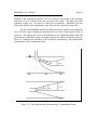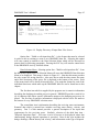
1
DROPMIX
User’s Manual
DRAFT
Prepared For:
Dr. Paul R. Schroeder
U.S. Army Engineer
Waterways Experiment Station
Vicksburg, MS 39180
Prepared By:
Don Chase, Ph.D, P.E.
Department of Civil & Environmental Engineering
University of Dayton
Dayton, OH 45469
November 1994
DROPMIX User’s Manual
Page i
Table Of Contents
PART 1: INTRODUCTION
Background . . . . . .
Purpose . . . . . . . . .
Scope . . . . . . . . . . .
.
.
.
.
.
.
.
.
.
.
.
.
.
.
.
.
.
.
.
.
.
.
.
.
.
.
.
.
.
.
.
.
.
.
.
.
.
.
.
.
.
.
.
.
.
.
.
.
.
.
.
.
.
.
.
.
.
.
.
.
.
.
.
.
.
.
.
.
.
.
.
.
.
.
.
.
.
.
.
.
.
.
.
.
.
.
.
.
.
.
.
.
.
.
.
.
.
.
.
.
.
.
.
.
.
.
.
.
.
.
.
.
.
.
.
.
.
.
.
.
.
.
.
.
.
.
.
.
.
.
.
.
.
.
.
.
.
.
.
.
Page
Page
Page
Page
1
1
2
2
PART 2: DREDGE DISCHARGE OPERATIONS AND THE MIXING ZONE Page 3
Dredging Overview . . . . . . . . . . . . . . . . . . . . . . . . . . . . . . . . . . . . Page 3
Open Water Disposal . . . . . . . . . . . . . . . . . . . . . . . . . . . . . . Page 4
Confined Disposal . . . . . . . . . . . . . . . . . . . . . . . . . . . . . . . . Page 5
Effect Of Disposal On The Environment . . . . . . . . . . . . . . . . . . . . . Page 6
Overview Of Hydrodynamic Mixing . . . . . . . . . . . . . . . . . . . . . . . . Page 6
Near Field Mixing . . . . . . . . . . . . . . . . . . . . . . . . . . . . . . . . Page 9
Far Field Mixing . . . . . . . . . . . . . . . . . . . . . . . . . . . . . . . . . Page 9
Application To Dredging Operations . . . . . . . . . . . . . . . . . . . . . . . Page 11
Dredge Discharge Mechanisms . . . . . . . . . . . . . . . . . . . . . . . . . . . Page 12
Pipeline Slurry Discharges . . . . . . . . . . . . . . . . . . . . . . . . . Page 12
Hopper Overflow Discharges . . . . . . . . . . . . . . . . . . . . . . . Page 13
CDF Effluent Discharges . . . . . . . . . . . . . . . . . . . . . . . . . . Page 13
Seepage From Confined Disposal Facilities. . . . . . . . . . . . . . Page 14
PART 3: DATA REQUIREMENTS AND PROGRAM OUTPUT
Program Limitations and Assumptions . . . . . . . . . . . . . . .
Input Data Requirements . . . . . . . . . . . . . . . . . . . . . . . .
Receiving Water Data . . . . . . . . . . . . . . . . . . . . . . . . . .
Dredged Material Disposal Operations Data . . . . . . . . . . .
Pipeline Slurry Discharge . . . . . . . . . . . . . . . . . . .
Hopper Overflow Discharges . . . . . . . . . . . . . . . .
CDF Effluent Discharges . . . . . . . . . . . . . . . . . . .
Seepage From Confined Disposal Facilities. . . . . . .
Dredge Discharge Orientation Data . . . . . . . . . . . . . . . . .
Pipeline Slurry Discharge . . . . . . . . . . . . . . . . . . .
Hopper Overflow . . . . . . . . . . . . . . . . . . . . . . . .
CDF Effluent Discharges . . . . . . . . . . . . . . . . . . .
Seepage From Confined Disposal Facilities . . . . . .
Mixing Zone Data . . . . . . . . . . . . . . . . . . . . . . . . . . . . .
Program Output . . . . . . . . . . . . . . . . . . . . . . . . . . . . . . .
.
.
.
.
.
.
.
.
.
.
.
.
.
.
.
.
.
.
.
.
.
.
.
.
.
.
.
.
.
.
.
.
.
.
.
.
.
.
.
.
.
.
.
.
.
.
.
.
.
.
.
.
.
.
.
.
.
.
.
.
.
.
.
.
.
.
.
.
.
.
.
.
.
.
.
.
.
.
.
.
.
.
.
.
.
.
.
.
.
.
.
.
.
.
.
.
.
.
.
.
.
.
.
.
.
.
.
.
.
.
.
.
Page
Page
Page
Page
Page
Page
Page
Page
Page
Page
Page
Page
Page
Page
Page
Page
15
15
16
17
20
21
22
23
24
26
27
28
28
29
33
34
DROPMIX User’s Manual
PART 4: . . . . . . . . . . . . . . . . . . . . . . . . . . . . .
Getting Started . . . . . . . . . . . . . . . . . . . .
The DROPMIX Environment . . . . . . . . . .
Selection Menus . . . . . . . . . . . . . . . . . . .
Activity Selection Menu . . . . . . . . .
Input Data File Selection Menu . . . .
Data Selection Menu . . . . . . . . . . .
Input File Saving Menu . . . . . . . . .
Execution Data File Selection Menu
DROPMIX Data Entry . . . . . . . . . . . . . . .
DROPMIX Data Requirements . . . . . . . . .
Project Title and Site Description . .
Receiving Water Data . . . . . . . . . .
Disposal Operations Data . . . . . . . .
Mixing Zone Data . . . . . . . . . . . . . . . . . .
Example Input Session . . . . . . . . . . . . . . .
Page ii
.
.
.
.
.
.
.
.
.
.
.
.
.
.
.
.
.
.
.
.
.
.
.
.
.
.
.
.
.
.
.
.
.
.
.
.
.
.
.
.
.
.
.
.
.
.
.
.
.
.
.
.
.
.
.
.
.
.
.
.
.
.
.
.
.
.
.
.
.
.
.
.
.
.
.
.
.
.
.
.
.
.
.
.
.
.
.
.
.
.
.
.
.
.
.
.
.
.
.
.
.
.
.
.
.
.
.
.
.
.
.
.
.
.
.
.
.
.
.
.
.
.
.
.
.
.
.
.
.
.
.
.
.
.
.
.
.
.
.
.
.
.
.
.
.
.
.
.
.
.
.
.
.
.
.
.
.
.
.
.
.
.
.
.
.
.
.
.
.
.
.
.
.
.
.
.
.
.
.
.
.
.
.
.
.
.
.
.
.
.
.
.
.
.
.
.
.
.
.
.
.
.
.
.
.
.
.
.
.
.
.
.
.
.
.
.
.
.
.
.
.
.
.
.
.
.
.
.
.
.
.
.
.
.
.
.
.
.
.
.
.
.
.
.
.
.
.
.
.
.
.
.
.
.
.
.
.
.
.
.
.
.
.
.
.
.
.
.
.
.
.
.
.
.
.
.
.
.
.
.
.
.
.
.
.
.
.
.
Page
Page
Page
Page
Page
Page
Page
Page
Page
Page
Page
Page
Page
Page
Page
Page
40
40
40
43
43
43
45
46
48
49
50
52
52
53
54
55
REFERENCES . . . . . . . . . . . . . . . . . . . . . . . . . . . . . . . . . . . . . . . . . . . Page 59
Appendix A List of DROPMIX Files . . . . . . . . . . . . . . . . . . . . . . . . . . Page A-1
DROPMIX User’s Manual
Page iii
List of Figures
Figure
Figure
Figure
Figure
Figure
Figure
Figure
Figure
Figure
Figure
Figure
Figure
Figure
Figure
Figure
Figure
Figure
Figure
Figure
Figure
Figure
Figure
Figure
Figure
Figure
2-1
2-2
2-3
2-4
2-5
2-6
3-1
Open-Water Dredge Disposal Methods . . . . . . . . . .
Examples Of Confined Disposal Facilities . . . . . . . .
Sewage Outfall Discharging Into A River . . . . . . . .
Example of a Pure Jet and a Pure Plume . . . . . . . . .
Velocity and Concentration Profile In The Near-Field
Example Of Buoyant Spreading . . . . . . . . . . . . . . .
CORMIX Representation of a Natural Channel
Cross-Section . . . . . . . . . . . . . . . . . . . . . . . . . . . .
3-2 Possible Receiving Water Density Profiles . . . . . . . .
3-3 Lateral Spreading Caused By Density Differences . . .
3-4 Dike Leakage Case . . . . . . . . . . . . . . . . . . . . . . . .
3-5 Examples of Horizontal and Vertical
Discharge Angles . . . . . . . . . . . . . . . . . . . . . . . . .
3-6 Pipeline Slurry Discharge Case . . . . . . . . . . . . . . . .
3-7 Channel Discharge Case. . . . . . . . . . . . . . . . . . . . .
3-8 Example of CORMIX X-Y-Z Coordinate System . . .
3-9 Three-Dimensional Representation of
Contaminant Plume . . . . . . . . . . . . . . . . . . . . . . .
4-1 Interrelationship Between DROPMIX Modules . . . . .
4-2 DROPMIX Activity Selection Menu . . . . . . . . . . . .
4-3 DROPMIX Input Data File Selection Menu . . . . . . .
4-4 Display Directory of Input Data Files Screen . . . . . .
4-5 DROPMIX Data Selection Menu . . . . . . . . . . . . . .
4-6 Example of Existing Data . . . . . . . . . . . . . . . . . . .
4-7 DROPMIX Input File Saving Menu . . . . . . . . . . . .
4-8 DROPMIX Execution Data File Selection Menu . . . .
4-9 Sample DROPMIX Spreadsheet For Data Entry . . . .
4-10 Project Title and Site Description Screen . . . . . . . .
.
.
.
.
.
.
.
.
.
.
.
.
.
.
.
.
.
.
.
.
.
.
.
.
.
.
.
.
.
.
.
.
.
.
.
.
.
.
.
.
.
.
.
.
.
.
.
.
.
.
.
.
Page 4
Page 5
Page 7
Page 8
Page 10
Page 10
.
.
.
.
.
.
.
.
.
.
.
.
.
.
.
.
.
.
.
.
.
.
.
.
.
.
.
.
.
.
.
.
Page
Page
Page
Page
16
18
21
25
.
.
.
.
.
.
.
.
.
.
.
.
.
.
.
.
.
.
.
.
.
.
.
.
.
.
.
.
.
.
.
.
Page
Page
Page
Page
26
27
29
38
.
.
.
.
.
.
.
.
.
.
.
.
.
.
.
.
.
.
.
.
.
.
.
.
.
.
.
.
.
.
.
.
.
.
.
.
.
.
.
.
.
.
.
.
.
.
.
.
.
.
.
.
.
.
.
.
.
.
.
.
.
.
.
.
.
.
.
.
.
.
.
.
.
.
.
.
.
.
.
.
.
.
.
.
.
.
.
.
Page
Page
Page
Page
Page
Page
Page
Page
Page
Page
Page
39
41
42
44
45
46
47
47
48
49
52
DROPMIX User’s Manual
Page 1
PART 1: INTRODUCTION
Background
Each year several hundred million cubic yards of sediment are removed from
rivers, waterways, ports, and harbors within the United States. The primary purpose of
these dredging activities is to maintain inland and coastal navigation and coastal defense
readiness. Given the nature of dredging operations, the processes involved in removing,
transporting, storing, and disposing dredged material must be carefully managed to insure
that dredging projects are completed in a cost-effective and environmentally safe manner.
Of central concern in dredging operations is the impact of discharges on the
receiving water environment. As such, the creation, migration, and dilution of a discharge
plume is of considerable interest as is the size of a required mixing zone for adequate
dilution. A mixing zone is a limited volume of water that serves as a zone of initial
dilution in the immediate vicinity of the point where material is discharged into the
receiving waters. Within this zone, the quality of the receiving waters, once mixed with
the discharged effluent, may not meet water quality criteria or standards otherwise
applicable to the receiving water. Most states limit the size of the mixing zone, and
hence the area where water quality standards may be violated, to as small a size as
practical. For example, 17 states restrict the size of the mixing zone in streams to 25%
or less of the stream’s cross-sectional area (USEPA, 1990).
Several mathematical models are available for estimating the growth and
movement of discharge plumes caused by subaqueous emissions. One of these models,
the Cornell Mixing Zone Expert System (CORMIX), was specifically developed to
provide a predictive tool for conventional or toxic pollutant discharges into waterways.
The CORMIX model focuses on the geometry and dilution characteristics of the initial
or near-field mixing zone. The CORMIX system consists of three separate modules: 1)
CORMIX1, 2) CORMIX2, and 3) CORMIX3. The CORMIX1 module is used to
examine submerged single port discharges, the CORMIX2 model is used to address
submerged multiport diffuser discharges, and the CORMIX3 program is used to analyze
surface discharges from channels.
The CORMIX model was originally developed to address bottom discharges with
low suspended solids concentrations. Such discharges are typically associated with
municipal wastewater or industrial waste outfalls. Dredged disposal operations, on the
other hand, typically involve surface or near-surface discharges with high suspended
solids concentrations. Consequently the existing CORMIX package is not directly
applicable. However, CORMIX may be used if surface discharges from dredge disposal
operations are made equivalent to the mirror image of bottom discharges. This
fundamental assumption is the foundation for the Dredging Operations Mixing Zone
Model (DROPMIX).
DROPMIX User’s Manual
Page 2
Instead of modifying the existing set of CORMIX programs to analyze surface or
near-surface discharges, a separate computer program was developed (Havis, 1994). This
preprocessor program takes data describing typical dredge discharge activities and
transforms the information into an equivalent mirror-image, bottom-discharge scenario
with sedimentation. As a result, the existing CORMIX models are used. However, some
slight modifications to the CORMIX output routines is necessary so that results can be
referenced back to the original geometry of the surface or near-surface discharge.
Purpose
To address the processes inherent in removal, transport, disposal, storage, and
general management of dredged material; the U.S. Army Corps of Engineers, Waterways
Experiment Station (USAEWES) has developed a computer package that assists engineers,
planners, and dredging operations managers in predicting the fate and behavior of dredged
material. The personal computer-based package is called ADDAMS - The Automated
Dredging and Disposal Alternatives Management System (Schroeder and Palermo, 1990).
ADDAMS consists of a number of individual computer programs, each of which performs
a unique function related to dredge material disposal or management. One of the
ADDAMS modules is the DROPMIX computer program.
This document serves as the User’s Manual for the DROPMIX computer program.
This manual will provide the necessary guidance so that data files describing various
dredge disposal operations can be created, executed, and interpreted. Specifically the
program is used to predict the fate and transport of dredged material discharges into a
receiving water environment. Results from the DROPMIX program typically consist of
the physical limits of the mixing zone and the concentration of pollutants within the zone.
It is assumed that users of the ADDAMS family of programs are already familiar with
dredging operations.
Scope
This document is subdivided into four parts. Part 1 provides a brief introduction
to the DROPMIX computer program. Part 2 gives a more thorough discussion of dredged
material disposal operations within the context of the DROPMIX program. Part 3
provides a summary of the data requirements and Part 4 addresses the particular data
format required by the DROPMIX program.
DROPMIX User’s Manual
Page 3
PART 2: DREDGE DISCHARGE OPERATIONS AND THE MIXING ZONE
Dredging Overview
Dredging is the act of removing or excavating sediments from the bottom of
bodies of water and is typically performed in order to maintain navigable channels in
inland and coastal waterways. Maintaining such channels helps to promote commerce and
national defense readiness. The dredging process typically refers to the removal,
transport, storage, and placement or disposal of dredged material. For any dredging
project, each element of the dredging process must be properly analyzed and designed and
the various components which comprise the project must be carefully coordinated to
insure a successful, cost-effective, and environmentally safe completion of the project.
Sediment can be removed from the bottom of a waterway either through hydraulic
or mechanical means. Hydraulic dredges remove sediment in a liquid slurry form through
use of a suction pump. The sediment is then pumped from the dredging site to a disposal
site or to a transportation vessel such as a hopper barge. Hydraulic dredges are generally
used for loosely compacted materials that are easily disturbed. As might be expected,
hydraulic dredges also transport large volumes of water through the slurry pipeline.
Because of the high water content associated with hydraulic dredging methods,
hopper dredges and scows used in these operations are occasionally filled past their rated
volume and are allowed to overflow. In such cases, the heavy material will quickly settle
to the bottom of the hopper while fine-grained material is held in suspension. The liquid
that is allowed to overflow will typically have a specific gravity very close to water, but
may also have a high turbidity (cloudy) and possibly high concentrations of pollutants if
the dredged sediment is contaminated. Consequently, environmental concerns may
preclude the use of hopper overflow to increase sediment loads.
Mechanical dredges remove bottom material through mechanical or physical
means. The material is excavated using backhoes, buckets, draglines, etc., lifted out of
the water, and typically placed into a temporary storage facility. Alternately, dredge
material may be placed directly into a permanent disposal facility if a suitable site can be
found in close proximity to the dredge site. Mechanical dredging activities exhibit the
desirable characteristic of removing very little water with the excavated material.
Consequently, excavated densities are very close to in-situ densities.
Regardless of how the dredge material is excavated, once the dredged material is
removed it must be disposed of in some fashion. There are three major alternatives for
dredged material disposal: 1) Open-water disposal, 2) Confined disposal, and 3)
Beneficial use. With regard to environmental impacts of disposal on receiving waters,
the open-water and confined disposal alternatives pose the greatest risk. As a result, they
are described in greater detail in the following paragraphs.
DROPMIX User’s Manual
Page 4
Open Water Disposal. Open-water disposal is the act of placing dredged
sediments within water bodies such as rivers, lakes, estuaries, or oceans as shown in
Figure 2-1. The dredged material may either be transported directly to the disposal site
via a pipeline or the material may be shipped to the site and released from hopper dredges
or barges. The discarded material is discharged at or very near the surface of the
receiving waters.
Figure 2-1 Open-Water Dredge Disposal Methods
Because dredged material is generally heavier than water, sediment that is disposed
of through open-water means will usually sink to the bottom. Material more dense than
the receiving water is said to be negative buoyant. Of course the material will not settle
to the bottom directly below the point of discharge. As shown in Figure 2-1, receiving
water currents may transport the material some distance away from the original discharge
point. In addition, the density of the receiving water can also influence the movement
of discharged material. Finally, the initial velocity associated with the effluent itself may
play a role in the final resting place for disposed sediments. The DROPMIX computer
program can be used to identify the extent over which material discharged into open
DROPMIX User’s Manual
Page 5
waters will migrate due to the receiving water environment and the nature of the openwater disposal method.
Confined Disposal. In some situations open-water disposal of dredged material
may not be feasible and the material must be stored in a confined disposal facility (CDF).
Generally a confined disposal facility is a man-made structure consisting of dikes which
enclose a specific disposal area. As shown in Figure 2-2, CDF’s may either be located
entirely on the shore (upland), adjacent to the shore (nearshore), or located away from the
shore (island). Several very large man-made islands are actually confined disposal
facilities for dredged material.
Figure 2-2 Examples Of Confined Disposal Facilities
Dredged material removed by hydraulic or mechanical means can be stored in a
CDF. However, because of the high water content associated with hydraulic dredging
methods, storage volumes will be greater than if material were excavated using
mechanical dredging methods.
DROPMIX User’s Manual
Page 6
Effect Of Disposal On The Environment
Depending upon the means by which dredged material is disposed, there can be
varying degrees of impact on the receiving water environment. For example, if a hopper
barge is allowed to overflow, then effluent - possibly contaminated, probably highly
turbid - will enter the receiving water causing a degradation of water quality in the
vicinity of the discharge point. If, on the other hand, a pipeline is used in an open-water
disposal project then the quality of the receiving water in the vicinity of the discharge
location and possibly at points further downstream will be affected, perhaps more than
in the hopper overflow case. Albeit small, even seepage from confined disposal facilities
can impact the quality of the receiving waters.
When discharges into a receiving body are made, a pollutant cloud or plume will
form. The discharge need not be toxic or highly polluted as suspended solids also
degrade water quality. The size, location, and movement of the plume, and hence the
impact on the receiving water, can be estimated using the DROPMIX model. In addition,
the program can be used to determine the extent of the mixing zone, that is, that area in
the immediate vicinity of the discharge point where water quality parameters may exceed
established criteria. Information describing the receiving water environment, the dredged
material disposal method, and the mixing zone is provided to the model. The model will
use this data in concert with numerical computations to generate information describing
the plume location, plume geometry, and pollutant concentration within the plume as a
function of time.
Overview Of Hydrodynamic Mixing
Consider a subaqueous outfall from a municipal wastewater treatment plant which
discharges into a water body as shown in Figure 2-3. A number of questions regarding
the discharge case can be asked. How far will the plume of significant concentration
move in the downstream direction? How far will the plume exceeding water quality
standards move laterally across the river’s cross-section? What is the concentration of
a specific pollutant 5, 50, or even 500 meters downstream of the discharge point? If the
stream is only 15 meters wide and the mixing zone is restricted to 25% of the stream’s
width, is this discharge case in compliance? Clearly a myriad of questions regarding the
geometric and pollutant characteristics of the discharge scenario can be asked not only
by design engineers but by regulating agencies as well.
Fortunately such questions can be answered with the assistance of mathematical
models, such as CORMIX, that have been specifically developed to address aqueous
discharges of this sort. The major variables needed to quantify the impact of the
discharge on the receiving water include:
DROPMIX User’s Manual
Page 7
Figure 2-3 Sewage Outfall Discharging Into A River
The
The
The
The
The
The
velocity of the receiving water,
velocity of the effluent,
density of the receiving water,
density of the effluent,
geometry of the receiving body of water,
geometry of the effluent discharge mechanism.
Discharges into a receiving stream may be subdivided into two fundamental
classes: a pure jet and a pure plume (Fischer, et al., 1979, Holley and Jirka, 1986). A
pure jet occurs when the discharge into the receiving environment is caused solely by the
momentum or velocity associated with the effluent. A pure plume, on the other hand, has
NO momentum affiliated with it. Rather the movement into the receiving environment
is due entirely to a difference in densities between the effluent and the receiving fluid,
i.e. one fluid is lighter than the other. A large number of discharges are a combination
of a pure jet and a pure plume. Discharges where both momentum and buoyancy play
a role in the shape and movement of the discharge plume are called buoyant jets or
forced plumes. Regardless of the mechanism by which effluent is introduced into the
receiving environment, the effluent will generally surge into the receiving fluid thereby
forming a cloud or plume.
DROPMIX User’s Manual
Page 8
Figure 2-4 Example of a Pure Jet and a Pure Plume
When effluent is released from a discharge mechanism (pipe, diffuser, etc.) the
momentum (velocity) affiliated with the effluent will typically dominate over the
receiving water velocity. Likewise, the distance the effluent column travels before
succumbing to the effects of the receiving water is also dependent upon the buoyancy
(density) of the effluent. Discharges that are lighter than water and hence move upwards
through the water column are said to be positively buoyant. The mixing that occurs in
the immediate vicinity of the outfall is dependent upon the characteristics of the effluent
and its discharge mechanism. The area where the momentum, buoyancy, and outfall
geometry control the shape and size of the discharge plume is termed the near field.
As the effluent plume rises, the initial momentum and buoyancy is dissipated and
the effects of the receiving water velocity and density become more pronounced. In fact,
the plume may begin to bend and will eventually start to disperse due to turbulence
associated with the receiving water. The region where the characteristics of the effluent
plume are governed by the receiving water environment is called the far field.
Once the far field region is encountered, the velocity of the receiving water
dominates and the effluent will, in most cases, begin to travel in a downstream direction.
In other words, the receiving water current will begin to carry the effluent away. For
DROPMIX User’s Manual
Page 9
most practical problems, the extent of the far field is much larger than that of the near
field. Of course the relative sizes of each field is dependent upon the particular discharge
and receiving water characteristics, but it is not uncommon for the limits of the near field
to be five percent or less of the far field. The CORMIX set of programs will identify
where the transition from the near field to the far field occurs.
Near Field Mixing. A very short distance from the outfall mechanism the effluent
will begin to mix with the receiving water. As the effluent mixes with the receiving
water, the concentration of any pollutants present within the effluent will begin to
decrease. In other words, the effluent will become diluted. As might be expected, the
concentration of any pollutant will generally decrease as the distance from the mouth of
the discharge mechanism increases. In fact, the dilution for a pure jet is linearly
proportional to the distance from the discharge point. For a pure plume, the dilution
varies with the distance squared. Thus for a buoyant jet, that is, a discharge case that has
both initial momentum and buoyancy, the pollutant concentration will decrease with
distance at a rate that varies between the rate for a pure jet and a pure plume.
Within the near field not only does the pollutant concentration decrease along the
plume trajectory, but the pollutant concentration also radiates outward perpendicular to
the trajectory as illustrated in Figure 2-5. Generally the concentration profile exhibits a
Gaussian or Normal probability distribution as it radiates outward from the trajectory
centerline. Regardless of the distance from the discharge point, the maximum
concentration can be found at the centerline of the plume trajectory and lower
concentrations normally exist at radial distances from the centerline.
Far Field Mixing. Once the effluent momentum has sufficiently dissipated, then
the effluent is said to be in the far field and far field mixing processes further dilute the
effluent pollutant concentration. There are two mixing processes at work in the far field
1) buoyant spreading and 2) passive diffusion. Buoyant spreading precedes diffusion and
is caused by the relative density differences of the now-mixed effluent and the receiving
waters. Doneker and Jirka (1990) indicate that four types of spreading may occur, an
example of which is shown in Figure 2-6.
1)
2)
3)
4)
Spreading
Spreading
Spreading
Spreading
at
at
at
at
the water surface,
the bottom,
a sharp internal density interface (pycnocline or thermocline),
the terminal level
However, if the effluent is nonbuoyant or weakly buoyant, or there are no
pronounced density differences within the receiving water, then buoyant spreading will
not occur and any additional mixing beyond the near fieldwill be due entirely to passive
diffusion. In other words, the turbulence associated with the receiving waters will cause
DROPMIX User’s Manual
Figure 2-5 Velocity and Concentration Profile In The Near-Field
Figure 2-6 Example Of Buoyant Spreading
Page 10
DROPMIX User’s Manual
Page 11
further dilution of the effluent.
Like near field mixing, mixing within the far field will occur in a longitudinal
direction parallel to the receiving water current and in a direction perpendicular to the
current. It is extremely important to point out that the geometry of the receiving water
plays a major role in far field mixing since it is possible that the effluent may come in
contact with and attach itself to the bank or receiving water bottom.
Application To Dredging Operations
The description of hydrodynamic mixing presented above is valid for subaqueous
bottom discharges that are commonly associated with point source emissions from
industry or municipalities. Dredging operations, on the other hand, involve discharges
that occur at or very near the receiving water surface. Fortunately the mixing behavior
of negatively buoyant surface discharges can be fully described by the physics of
positively buoyant bottom discharges. The fundamental assumption which allows bottom
discharges to be used to model surface discharges can be stated as follows.
Negatively-Buoyant Surface Discharges = The Mirror Image of
Positively-Buoyant Bottom Discharges
In order for results to be meaningful, however, the boundary conditions of the surface
discharge problem must be transformed to remain consistent with the equivalent boundary
conditions for the bottom discharge problem.
This is the approach taken in the DROPMIX computer model. The mixing
characteristics of surface or near-surface dredge-related discharges into receiving waters
are modeled by transforming the problem into an equivalent bottom discharge problem.
This is accomplished by creating a mirror image of the surface discharge problem using
a preprocessor program (Havis, 1994). The preprocessor program generates a data file
representing the equivalent bottom discharge case for the CORMIX model. CORMIX
analyzes the bottom discharge case to generate information on the mixing zone and
pollutant plume. This information includes the location and concentrations of effluent
within the receiving waters.
The majority of effort required to transform a surface discharge case into an
equivalent mirror image bottom discharge scenario is affiliated with the effluent and
receiving water densities. For the CORMIX routines, receiving water density profiles are
referenced to the receiving water bottom. However for dredged material disposal, density
differences are referenced to the water surface. Also the CORMIX programs reference
step density changes to the bottom. Once again a transformation must be made to
reference any step changes to the surface.
DROPMIX User’s Manual
Page 12
Dredge Discharge Mechanisms
Six types of surface or near-surface discharges are accommodated by the
DROPMIX program. Each discharge case is described in greater detail in the following
paragraphs.
1)
2)
3)
4)
5)
6)
Pipeline Slurry Discharges
Hopper Overflow Discharge - Single Port
Hopper Overflow Discharge - Weir Flow
CDF Effluent Discharge Via Channel/Side Stream
CDF Effluent Discharge Via Pipe
Containment Dike Leakage
Pipeline Slurry Discharges. A common disposal method, particularly for openwater disposal operations, is to discharge dredged material through a pipeline. Pipeline
discharges of this sort are most commonly used in concert with hydraulic dredging
operations. The pipeline transports the dredged slurry a reasonable distance from the
dredging site to a location where its deposition will not interfere with navigation or other
uses of the water body. Effluent from a pipeline will typically have a much higher
concentration of suspended solids than the receiving water. The effluent could also
contain heavy metals, toxins, or other pollutants that have previously settled to the bottom
of the dredged channel and adsorbed to the sediment.
When effluent discharges from a pipeline, it will typically find its way to the
bottom of the receiving water. This may be accomplished by directing the outlet of the
effluent pipe downwards towards the bottom of the receiving waters. More likely,
however, the nature of the negatively buoyant effluent will cause the material to sink to
the bottom. Regardless of the bottom-forcing mechanism, when the effluent plume strikes
the bottom, it will begin to disperse or fan-out. Furthermore, the momentum associated
with the sinking effluent could disturb dredged material which has previously settled to
the bottom thus increasing the size of the dispersion plume.
The approach used to model pipeline discharges and subsequent bottom collapseinduced mixing involves use of both the CORMIX1 and CORMIX2 modules. That
portion of the mixing from the mouth of the pipeline to the receiving water bottom is
modeled using the CORMIX1 program within a mirror image framework. Any
subsequent mixing that occurs after the plume strikes the bottom is modeled assuming
that the flow resembles flow though a multi-port diffuser. Thus the CORMIX2 module
is used; however, in this case there is no mirror image transformation since the discharge
originates at the bottom of the receiving water.
DROPMIX User’s Manual
Page 13
Hopper Overflow Discharges. As mentioned previously, a hopper barge may be
allowed to overflow in order to increase the sediment load carried by the vessel. This has
proven to be an effective method for coarse-grained sediments although for fine-grained
material the effectiveness of this approach is questionable (USACE and USEPA, 1992).
When the barge overflows, sediment-laden water leaves the vessel and enters the
receiving water. Not only is the effluent likely to have a higher turbidity than the
receiving water, but because it has been in contact with the dredged material it may also
have trace concentrations of heavy metals, toxins, or other pollutants.
Hopper barges typically overflow in an uncontrolled manner. The flow may be
over one or more sides of the vessel and generally resembles flow over a weir. In some
cases, the flow over the sides is collected and routed to a common point where it is
discharged through a single pipe. When a hopper is used in conjunction with hydraulic
dredge operations a steady-state condition may assume to exist. In other words, the flow
rate over the sides of the barge is equal to the rate at which sediment is pumped to the
vessel. The assumption of steady-state conditions is made in the DROPMIX program for
the hopper overflow case. For the single port discharge, hopper overflow is modeled
using the CORMIX1 program; whereas, CORMIX2 is used for uncontrolled weir-type
discharges. In both instances, however, a mirror image transformation is made.
CDF Effluent Discharges. Confined disposal facilities are engineered structures,
and as such, they are typically equipped with outlet devices that decant excess water
generated by the hydraulic dredging process. An example of such an outlet structure
would be a culvert passing through the dike face. Because the excess water comes in
contact with the disposed material, it is possible that the effluent has higher concentrations
of suspended solids or other pollutants than the receiving water. Usually the outlet
structure represents a single point discharge and as a result the CORMIX1 module may
be used. For effluent discharges from confined disposal facilities via a single pipe,
DROPMIX uses the CORMIX1 module with a mirror-image transformation.
For upland CDF’s, that is, those structures that are not located adjacent to open
waters; the effluent is usually discharged into a receiving stream having little or no
continuous flow. In fact, the discharge from the CDF may represent the greatest fraction
of flow within the stream. The stream, in turn, typically discharges into a much larger
body of water such as a river, estuary, or ocean. Like pipeline discharges, hopper
overflows, and direct CDF discharges, channel discharges can also degrade receiving
water quality. The CORMIX3 module is used to analyze channel or side stream
discharges from upland containment facilities. CORMIX3 was developed specifically to
evaluate aqueous mixing of surface discharges and, as a result, no modifications of the
discharge scenario is necessary.
DROPMIX User’s Manual
Page 14
Seepage From Confined Disposal Facilities. When a confined disposal facility is
used to store dredged material, the material may initially have a high water content
especially if used in hydraulic dredging operations. Although the sediment may
eventually dewater (dry out), a combination of factors including hydraulic gradients,
weight of the sediment, and porosity of the dike will cause effluent to leak from the
containment facility. In addition, infiltrated precipitation will recharge the zone of
saturation such that leakage from the facility may continue long after the initial sediment
moisture content has decreased.
Admittedly the flow or velocity through the CDF’s porous dikes will be small and
occur over very large distances compared to the other disposal cases described above.
Nonetheless, the flow through the CDF can degrade water quality and as a result merits
examination. In DROPMIX, flow through a porous dike is modeled assuming that the
dike acts as a multi-port diffuser. Consequently, the CORMIX2 module is used to predict
pollutant concentrations within the receiving water.
DROPMIX User’s Manual
Page 15
PART 3: DATA REQUIREMENTS AND PROGRAM OUTPUT
Program Limitations and Assumptions
In order for CORMIX to accurately simulate subaqueous discharges, the effluent
must represent a continuous steady-state discharge. In addition, steady-state flow within
the receiving water must exist. Of course the condition of continuous flow is relative to
the time over which mixing occurs. For example, a hopper overflow will not be "truly
continuous". Operations - and hence discharges into the receiving water - will cease after
the hoppers have filled. However, the duration over which overflow occurs, on the order
of hours, is typically much larger than the duration over which initial dilution occurs, on
the order of minutes or even seconds. Moreover, the travel time within the regulatory
mixing zone is typically less than one hour. Furthermore, a second barge may begin to
overflow relatively shortly after the first barge thus preserving the assumption of
continuous flow. Consequently the assumption of continuous discharge is assumed to be
valid.
With regard to the assumption of steady-state flow, flow through a pipeline or over
a weir will not be "truly steady" due to minor variances in the flow rate. However, the
time over which these variances occur is generally small compared to the time over which
mixing occurs. Thus the assumption of steady-state flow is assumed to hold. Not only
is the flow presumed to be steady, but the receiving water velocity is assumed to be
uniform, that is, the velocity exhibits the same magnitude everywhere over its entire
cross-section.
Changes in receiving water velocities associated with tidal effects may be ignored
since these occur over much longer periods of time than mixing occurs (hours vs.
minutes). Alternatively, if long-term mixing results are desired, then it is possible to
conduct a quasi-steady analysis. Typically in these cases the results from prior steadystate analyses are used as boundary or initial conditions for subsequent analyses.
Mixing within the receiving water is assumed to be due solely to hydrodynamic
processes. In other words, dilution of the effluent concentrations is assumed to be the
result of the interactions between effluent and receiving water velocities, densities, and
geometries. The original CORMIX modules assume that the pollutant is a conservative
species and that any physical, chemical, or biological reactions or decay processes do not
exist. However, modifications to the program have incorporated first-order reaction
processes (Havis, 1994). Field studies suggest that results of CORMIX simulations
accurately predict the mixing and the subsequent migration of contaminant plumes
(Doneker and Jirka, 1990).
DROPMIX User’s Manual
Page 16
CORMIX assumes that regardless of its natural cross-section, the receiving water
body can be modeled as a rectangular channel as shown in Figure 3-1. For many
artificial waterways and well-channelized natural streams, this assumption is clearly valid
and hence selection of receiving water geometry (channel width and depth) is rather
straightforward. However for natural streams having irregular cross-sectional geometry,
selection of this data is not as apparent. Consequently, engineering judgement plays a
major role in identifying channel geometry. The astute program user will conduct
multiple simulations varying channel geometry to obtain an intuitive feel for the
sensitivity between model input and output.
Figure 3-1 CORMIX Representation of a Natural Channel Cross-Section
Input Data Requirements
The primary function of DROPMIX is to analyze mixing of effluent from dredging
operations discharging into inland and coastal waterways and at ocean dumping sites.
The model can accommodate six discharge scenarios:
1)
2)
3)
4)
5)
6)
Pipeline Slurry Discharges
Hopper Overflow Discharge - Single Port
Hopper Overflow Discharge - Weir Flow
CDF Effluent Discharge Via Channel/Side Stream
CDF Effluent Discharge Via Pipe
Containment Dike Leakage
DROPMIX User’s Manual
Page 17
Given information describing the receiving water conditions, the characteristics of
the effluent and the manner in which it is disposed, and general information on initial
pollutant concentrations; DROPMIX will determine the dilution characteristics of the
effluent-receiving water environment.
Program output includes the centerline
concentration of a pollutant along the trajectory of the contaminant plume and the degree
of lateral dispersion perpendicular to the plume trajectory.
DROPMIX utilizes the CORMIX suite of computer programs to analyze mixing.
Since discharges associated with dredging operations typically occur at or very near the
surface, a mirror image transformation is made. Using a numerical preprocessing
program, a negatively-buoyant surface discharge is converted to an equivalent positivelybuoyant bottom discharge. This mirror image discharge is then analyzed by the CORMIX
modules. Modifications to the output routines in the CORMIX programs have been made
so that program output is referenced to the surface.
The data required to perform a complete mixing zone simulation can essentially
be subdivided into three categories:
1) Data describing the receiving water environment,
2) Data describing the effluent and its discharge mechanism,
3) Data describing the mixing zone.
Each of the individual data requirements are described in greater detail in the following
paragraphs.
All data supplied to the DROPMIX program must be
given in METRIC units.
Receiving Water Data
There are three major data items which fully describe the receiving water
environment: 1) density, 2) velocity, and 3) geometry. CORMIX will determine if an
effluent plume comes in contact with or attaches to a boundary such as the bank of a
river or the bottom of a lake. Consequently information describing the presence of
boundaries, receiving water depths, bottom roughnesses, and degree of channel
meandering are required. Also required are the mean channel velocity and mean wind
speed. Finally data describing the receiving water density profile must be provided.
The receiving water may exhibit one of three density profiles: 1) Uniform, 2)
Linearly varying, or 3) a Two-Layer or Pycnocline profile. For the uniform profile, the
receiving water density is assumed to remain constant throughout its depth. With the
DROPMIX User’s Manual
Page 18
linear profile, on the other hand, density is assumed to vary linearly from the surface
density to the bottom density as illustrated in Figure 3-2. The final density profile
assumes a uniform two-layer density separated by a step located a specified distance from
the receiving water bottom. Density information may be specified directly or computed
by the program based on user-specified depth, salinity, and temperature.
Figure 3-2 Possible Receiving Water Density Profiles
Receiving water velocity is specified directly by the program user. It is assumed
that information on channel velocities would be more readily available than data
describing receiving water discharges. The specified velocity represents the mean velocity
acting uniformly over the width and depth of the receiving water body. In addition, the
velocity is assumed to be constant over the duration of the simulation. The mean wind
speed must also be specified to account for mixing effects from wind-induced turbulence.
DROPMIX allows users to indicate if the wind speed is low, medium, or high.
Depending upon the wind conditions specified by the program user, DROPMIX will
assign a value of 0 m/s, 2 m/s, or 15 m/s respectively to the wind speed.
CORMIX has the ability to indicate if the effluent plume comes in contact with
and attach to the receiving water banks or bottom. Obviously the potential for bank
contact and attachment is higher for narrow channels, such as rivers and streams, than for
wider bodies of water, e.g. lakes, bays, and coastal areas. In addition, diffusivity
coefficients - which control far-field mixing - differ for narrow and wide water courses.
DROPMIX User’s Manual
Page 19
Thus CORMIX requires information on whether the receiving water is bounded. As the
name implies, a bounded channel is one where the receiving water channel is bounded
on both sides by banks. Examples of bounded channels include rivers, streams, or even
narrow harbors. Examples of unbounded channels include wide lakes, estuaries, and
coastal areas. In some cases it may not be clear whether the receiving water is bounded
or unbounded. Under these circumstances the program-user should perform multiple
simulations assuming bounded and unbounded conditions and make appropriate
engineering decisions accordingly.
Receiving water geometry is also described by the average or mean depth and the
bottom roughness. As mentioned previously, CORMIX assumes that the receiving water
body can be characterized as a rectangular channel. Thus the depth specified by the
program user represents the depth of the rectangular section. Bottom roughness values
may be specified either in terms of Manning’s "n" value or a Darcy-Weisbach friction
factor "f". Table 3-1 lists receiving water variable names and a brief description of their
meaning.
Table 3-1 Description of Receiving Water Variables
Variable
Name
Description
Notes
CBOUND
Indicates if receiving body of water is bounded
ICHREG
Indicates degree of channel meandering
1
BS
Width of rectangular channel cross-section
1
HA
Mean depth of rectangular channel cross-section
MANN
F
Manning’s "n" for bottom roughness
2
Darcy-Weisbach friction factor "f" for bottom roughness
2
UA
Mean velocity of receiving water
UW
Mean wind speed
STRCND
Indicates type of density profile
RHOA
Density for Uniform density profile
RHOAS
Surface density for Linear or Two-Layer density profile
RHOAB
Bottom density for Linear or Two-Layer density profile
HINT
Distance from bottom of water body where density step occurs
3
4
DROPMIX User’s Manual
Page 20
Notes:
1) If the receiving water body is unbounded, then the degree of channel
meandering and the width of the channel does not have to be specified. These variables
are only applicable to for bounded channels.
2) The user must specify either Manning’s roughness "n" or Darcy-Weisbach
friction factor "f". If Manning’s "n" is given, then the preprocessor will convert it to an
equivalent Darcy-Weisbach friction factor.
3) The following convention is adopted for density profiles:
U - Uniform Density Profile
A - Linearly-Varying Density Profile
B - Two-Layer or Pycnocline Density Profile
4) The distance above the receiving water bottom where the pycnocline occurs
must only be specified for a Two-Layer or Pycnocline Density Profile.
Dredged Material Disposal Operations Data
Dredged material disposal data generally refers to the physical characteristics of
the discharged effluent and its discharge mechanism. As mentioned earlier, six dredged
material disposal mechanisms can be analyzed with DROPMIX. Although there is certain
data that is unique to each discharge case, the information required to describe the
dredging operations environment is very similar to that of the receiving water.
Information needed to fully describe the disposal operations are: 1) effluent density, 2)
effluent velocity, 3) geometry of the effluent discharge device, and 4) orientation of the
effluent discharge mechanism with respect to the receiving water current.
Unlike the receiving water, the dredge effluent is not allowed to have multiple
densities. The density of the effluent is initially assumed to be greater than the surface
density of the receiving water so as to preserve negatively buoyant conditions. This will
typically result in the effluent continuing to sink to the receiving water bottom even after
the initial effluent momentum is dissipated. However, it is possible that as the effluent
plume migrates towards the bottom, the density of the diluted effluent and the density of
the surrounding water will converge. Under these circumstances it is possible that the
effluent plume will cease to move downward and will begin to disperse laterally in a
direction parallel to the channel bottom as shown in Figure 3-3. CORMIX will model
lateral spreading of this sort. Within the DROPMIX program, effluent density may be
specified directly, or computed based on user-supplied data describing the effluent fluid
density and the concentration and density of solids within the effluent.
DROPMIX User’s Manual
Page 21
Figure 3-3 Lateral Spreading Caused By Density Differences
In addition to the effluent density, DROPMIX requires the user to supply the
velocity of the effluent exiting from the discharge mechanism. In a practical sense the
velocity of flow over the sides of a barge or through a dike, pipeline, or channel is rarely
known. What is typically known, however, is the effluent flow rate. Consequently,
DROPMIX does not allow entry of effluent velocities. Rather an effluent discharge rate
is required and the program will convert the user-provided flow rate into an equivalent
velocity using the continuity equation shown below:
(1)
where:
U0 = Effluent Velocity (m/s)
Q0 = Effluent Discharge (m3/s)
A0 = Area Over Which Discharge Occurs (m2)
Pipeline Slurry Discharge. Concerning effluent velocities, the pipeline slurry
discharge case requires data that quite possibly is the easiest of the six discharge cases
to obtain. The user must specify the flow rate through the pipeline. Since pipeline
discharges are most frequently used in hydraulic dredging operations, the pipeline flow
DROPMIX User’s Manual
Page 22
rate may assumed to be equal to the hydraulic dredge pumping rate. The program user
must also specify the diameter of the pipe. The effluent velocity is then easily found by
employing the continuity equation.
The pipeline slurry discharge case is simulated in DROPMIX as a combination of
a single port discharge followed by a multi-port diffuser discharge. Consequently,
information describing the physical characteristics of the multi-port diffuser must be
provided. Diffuser information includes the length of the diffuser, the number of diffuser
ports, and the diameter of each port.
Hopper Overflow Discharges. For the hopper overflow case, the rate at which
effluent leaves the barge is assumed to be equal to the pumping rate of the hydraulic
dredge. Hopper overflows resulting from mechanical dredging operations should not be
simulated with the DROPMIX model. Receiving water effects from barge, scow, or other
vessel overflows are found assuming that effluent leaves the vessel as: 1) weir flow or
2) flow through a single pipe or port.
As mentioned previously, hoppers are frequently allowed to overflow in order to
increase the sediment load carried by the vessel. Usually the overflow is uncontrolled,
that is, flow is allowed to spill over one or more sides of the vessel. In some cases,
however, the overflow is captured and routed to a common point on the vessel where it
is then discharged, generally through a pipeline, into the receiving waters. For overflow
discharged through a single port, the velocity of the effluent is found using the continuity
equation assuming that the port is a circular pipe. As a result, the user must supply the
overflow rate and the diameter of the pipe.
DROPMIX can also simulate uncontrolled overflows assuming that the flow acts
as weir flow. Once again the continuity equation may be used to determine the effluent
velocity; however, the unknown in this case is the area over which flow occurs. If the
overflow rate and the length over which flow occurs is known, then the height or head
above the "weir" can be found by the weir equation:
(2)
where:
Hw = Height of Effluent Above the Weir (m)
Q0 = Effluent Discharge (m3/s)
L0 = Hopper Overflow Length (m)
Cw = Weir Coefficient ≈ 1.88
Once the height above the weir is known, then the flow area is simply the product
of the overflow length, L0, and the weir height as shown below:
DROPMIX User’s Manual
Page 23
(3)
CDF Effluent Discharges. DROPMIX assumes that direct effluent discharges, not
seepage, from confined disposal facilities is either routed immediately to the receiving
water through a single pipeline or is transported through a channel or side stream for
ultimate disposal into the receiving waters. In either case, the velocity of the effluent is
required in order to perform the mixing zone simulation.
For the case of CDF effluent disposal via a pipeline, DROPMIX requires the
program user to supply data on the discharge from the CDF and the diameter of the
pipeline. This information is used with the continuity equation to determine effluent
velocity. Discharge from a CDF will primarily be due to displacement of supernatant by
the dredged discharge and can generally be assumed to be equal to the rate at which
material is discharged into the CDF, i.e. steady-state conditions. Use of the continuity
equation shown in Eq. (1) implies that the pipeline is flowing full during discharge
events.
The velocity within a stream or open channel can also be found using the
continuity equation. The program user must supply the channel discharge and geometry.
For the case of a side stream, the discharge within the waterway can be found from a
hydrologic analysis of the CDF and any surrounding areas which contribute flow to the
channel.
Two types of open channels are supported by the DROPMIX program: 1)
rectangular channels and 2) circular pipes. For the rectangular channel, the channel width
and depth of flow must be provided. The product of these two quantities is the flow area
which is used in the continuity equation to obtain the effluent velocity. For circular
pipes, the pipe diameter and depth of flow are specified by the program user.
DROPMIX treats circular pipes flowing partially full as rectangular channels with
comparable depths and cross-sectional areas. For a set of given pipe characteristics
(diameter and depth of flow), one may determine a congruent rectangular channel by
equating the area of both sections and solving for the depth of flow in the rectangular
channel. For a given discharge, the equation below provides an expression for the flow
depth in a rectangular channel which will have the same area and velocity as a pipe
flowing partially full.
(4)
where:
ych = Depth of Flow in a Rectangular Channel (m)
B = Width of Rectangular Channel (m)
DROPMIX User’s Manual
Page 24
D = Pipe Diameter (m)
θ = Central Angle (rad) = cos-1(1-2yp/D)
yp = Depth of Flow in a Circular Pipe (m)
Eq. (4) will allow an equivalent depth in a rectangular channel, ych, to be
computed based on a pipeline that is flowing partially full at a depth of yp. However, in
order to compute ych, the width of the rectangular channel, B, - which is not known must be supplied. Consequently the program user must supply an assumed value for the
rectangular channel bottom width and compute the depth of flow accordingly. The
approach outlined above will insure that the velocity in the rectangular section is the same
as the velocity in the circular pipe for the same effluent discharge rate. This is key since
effluent velocity and not effluent discharge is the critical parameter in evaluating
receiving water quality effects.
Channels used to transport releases from upland CDF’s to receiving waters may
be natural or man-made. In either case, it is quite possible that the channel will not
exhibit a true rectangular shape. Under these circumstances, an equivalent rectangular
cross-section must be provided. An analysis similar to the one described above can be
used. The cross-sectional area of the actual channel and a rectangular channel are equated
and solved assuming a fixed bottom width. The solution will provide the flow depth such
that both channels have the same velocity.
Seepage From Confined Disposal Facilities. For the case of leakage from a
confined disposal facility, the user must specify the total discharge through all porous
dikes which contribute flow to the receiving waters. However, this may not include each
and every side of the facility. At present, CORMIX is unable to model counter-flowing
discharges, that is, discharges where the effluent direction is opposite the receiving water
direction. Figure 3-4 shows a three-sided nearshore CDF used to store dredged material.
Of the three sides, side A opposes the current; whereas, sides B and C do not.
Consequently, the discharge supplied to the DROPMIX model must reflect the seepage
through sides B and C. It is the responsibility of the program user to supply accurate
estimates of flow through the porous dike. One possibility is to employ Darcy’s Law or
use flow nets to estimate leakage through the contributing sides of the facility.
Leakage through a porous dike is modeled with the CORMIX2 module assuming
that flow through the dike behaves similarly to flow through a multi-port diffuser. As a
result, information describing the multi-port diffuser must be provided - namely the
number of diffuser ports, the diameter of the individual ports, and the length of the
diffuser. It is assumed that each port has the same diameter.
Because of the wide variability in potential diffuser characterization and the
somewhat unwieldy data requirements associated with diffuser depiction, DROPMIX takes
a simplistic approach when describing diffusers used to simulate dike leakage. First, the
DROPMIX User’s Manual
Page 25
Figure 3-4 Dike Leakage Case
number of diffuser ports is assumed to be 10,000. Secondly, the velocity of the effluent
seeping from a CDF is assumed to be 0.02 m/s. Using this information with the total
leakage rate, the diameter of the individual diffuser ports can be found from the equation
below. The length of the diffuser may be specified directly or can be determined
automatically by the program. The next section provides details on diffuser lengths.
(5)
where:
D0 = Diffuser Port Diameter (m)
QT = Cumulative Discharge Through Porous Dikes (m3/s)
U0 = Effluent Velocity = 0.02 m/s
NP = Number of Diffuser Ports = 10,000
DROPMIX User’s Manual
Page 26
Dredge Discharge Orientation Data
The final component of dredged material disposal data is the orientation of the
discharge mechanism. CORMIX requires information describing the positioning of the
discharge mechanism in relation to the receiving water current. Although the particular
data which must be supplied is dependent upon the particular discharge case, each of the
six cases requires information describing the vertical and horizontal discharge angles.
The vertical discharge angle, Θ, is the angle in the X-Z plane the effluent device
centerline makes with the receiving water surface. An angle of 0o reflects a discharge
case where flow is parallel to the water surface. A value of 90o indicates that flow is
oriented vertically downwards; whereas, a value of -45o refers to the case where discharge
is occurring upwards at an angle of 45o with the water surface. The horizontal angle, σ,
is the angle in the X-Y plane measured with respect to the receiving water current. Thus
an angle of 0o indicates a co-flowing case where flow is parallel to the current, while a
value of 180o describes a counter-flowing case, i.e. flow directly opposes the prevailing
current. Horizontal angles of 90o and 270o reflect cross-flow conditions where the
effluent is discharged perpendicular to the receiving water current. Figure 3-5 illustrates
the vertical and horizontal discharge angles used in the DROPMIX program.
Figure 3-5 Examples of Horizontal and Vertical Discharge Angles
DROPMIX User’s Manual
Page 27
Pipeline Slurry Discharge. The pipeline discharge case is simulated assuming a
single port discharge followed by a multi-port diffuser discharge. Consequently, the
information needed to describe the orientation of the discharge mechanisms are the
vertical and horizontal discharge angles of the pipeline, and the vertical, horizontal, and
diffuser axis angles describing the diffuser. Figure 3-6 depicts the angles necessary to
fully describe the orientation of the pipeline discharge case.
Figure 3-6 Pipeline Slurry Discharge Case
Note in Figure 3-6, that the distance between the pipeline outlet and the diffuser,
DISTPD, is needed. This length represents the horizontal distance the effluent will travel
before it strikes the bottom of the receiving water channel. This distance may be found
using vector analysis. The composite velocity in the same direction as the effluent stream
is a function of the effluent velocity, the receiving water velocity, and the horizontal and
vertical discharge angles. The expression below can be used to compute this velocity.
(6)
DROPMIX User’s Manual
where:
Page 28
UDISTPD = Horizontal Effluent Velocity (m/s)
UA
= Receiving Water Velocity (m/s)
= Effluent Velocity (m/s)
U0
Θ
= Vertical Discharge Angle (rad)
σ
= Horizontal Discharge Angle (rad)
The time required for the effluent plume to travel from the pipeline to the
receiving water bottom is found from Eq. (7). Once the travel time is known, it is
multiplied by the composite velocity, UDISTPD, to find the distance traveled, DISTPD.
(7)
where:
t
= Time For Effluent To Travel From Pipeline To Channel
Bottom (sec)
U0 = Effluent Velocity (m/s)
Θ = Vertical Discharge Angle (rad)
Hd = Mean Receiving Water Depth at Discharge Location (m)
Hopper Overflow. For the hopper overflow case, the only geometric information
needed to fully describe the discharge orientation are the vertical and horizontal discharge
angles and the distance below the water surface where effluent enters the receiving water.
If overflow is through a single port, then the vertical angle is the angle the pipe makes
with the water surface and the horizontal angle is the angle the pipeline makes with the
receiving water current as shown in Figure 3-5. If, on the other hand, overflow is
simulated as weir flow then the user must specify the vertical discharge angle and the
angle the vessel makes with the receiving water current. Typically for weir flow the
vertical angle will be 90o. Based on the angle the vessel makes with the current,
DROPMIX automatically computes the remaining necessary discharge angles.
In certain discharge cases, the barge may be moving as it releases dredged
material. This factor is considered by using vector analysis. Using the horizontal
discharge angle, the vessel velocity can be decomposed into two components - one
component acting in the same direction as the receiving water and another component
which is orthogonal to the receiving water direction. A composite velocity, acting in the
same direction as the receiving water current, is then found by adding the receiving water
current to the velocity component acting in the same direction as the receiving water.
CDF Effluent Discharges. The geometric information needed for direct discharges
from a CDF are dependent upon how discharge from a confined disposal facility is
modeled. If flow is assumed to enter the receiving water from a single pipeline, then
only the vertical and horizontal discharge angles are needed. Figure 3-5 portrays this
information.
DROPMIX User’s Manual
Page 29
If CDF discharge is modeled as a channel or side stream discharge, then three
variables are needed to fully describe the orientation of the channel with respect to the
receiving water. The first variable is a horizonal angle that the channel centerline makes
with the receiving water current. The second variable is the slope of the receiving water
bottom. This quantity represents the change in receiving water bottom elevation from the
point where the channel discharges to the point where the average receiving water depth
is reached. Finally, the distance the channel protrudes out into the receiving water must
be supplied. Each of the geometric variables described above are shown in Figure 3-7.
Figure 3-7 Channel Discharge Case.
Seepage From Confined Disposal Facilities. The geometric description of the dike
leakage case is somewhat more involved than the hopper overflow or CDF discharge
cases due to the presence of multiple diffuser ports. As before, the vertical and horizontal
discharge angles for the diffuser ports must be specified. In addition, the orientation of
the dike itself in relation to the receiving water current must be provided. Assuming that
the individual discharge ports are perpendicular to the dike axis, a relationship between
the port discharge direction and dike axis angles exists as shown below:
DROPMIX User’s Manual
Page 30
(8)
where:
σ = Horizontal Discharge Angle (deg)
γ = Dike Axis Angle (deg)
For confined disposal facilities with multiple faces, a single equivalent dike face
is assumed to discharge effluent. The user is required to supply the maximum distance
the CDF extends out into the receiving water and the width of the facility. DROPMIX
will then compute the dike axis angle, γ, using the following equation:
(9)
where YB1 is the maximum distance the CDF extends out into the receiving water (m)
and width is the maximum width of the disposal facility. The equivalent dike length is
found from:
(10)
Recall that dike faces which oppose the flow should not be included in the analysis. A
list of the variables required to completely describe the dredged material disposal
environment are provided in Table 3-2.
DROPMIX User’s Manual
Page 31
Table 3-2 Description of Dredged Disposal Variables
Variable
Name
CBANK
DISTB
DISTPD
Description
Notes
Bank closes to point of discharge
Distance from CBANK to point of discharge
Distance between pipeline discharge and diffuser
Data Required For Hopper Overflow, Dike Leakage, and Pipeline Discharge Case
THETA
Horizontal angle between effluent trajectory and receiving
water current
SIGMA
Vertical angle between effluent trajectory and receiving water
current
H0
Depth from surface to point of discharge
HD
Depth of receiving water at discharge location
Diffuser Data For Dike Leakage and Pipeline Discharge Cases
DITYPE
BETA
Type of diffuser
Angle between diffuser discharge direction and diffuser axis
GAMM
A
Angle between diffuser axis and receiving water current
THETA2
Horizontal angle between diffuser effluent trajectory and
receiving water current
SIGMA2
Vertical angle between diffuser effluent trajectory and
receiving water current
H02
Depth from surface to point of discharge for diffuser
SPAC
Spacing of diffuser ports for dike leakage case
PORTN
Number of diffuser ports in dike leakage case
D02
Diameter of diffuser ports in dike leakage case
LD
Dike Length
YB1
Maximum distance dike extends out into receiving water
DROPMIX User’s Manual
Page 32
Table 3-2 (Cont.)
Variable
Name
Description
Channel Data For Open Channel Flow Case
CHNTY
P
Type of open channel: Rectangular or Pipe
BO
Width of rectangular channel
HO
Depth of flow in open channel
YO
Distance channel protrudes into waterway
THETA
B
SIGMAC
Slope of receiving water bottom
Horizontal angle of discharge
Hydraulic Data Required For All Four Cases
Q0
Effluent discharge rate
A0
Area over which effluent is discharge
D0
Diameter of single port discharge pipe
RHO0
Effluent density
RE2D
Reynolds number
Q0T2D
Total flow through dikes
Notes
DROPMIX User’s Manual
Page 33
Mixing Zone Data
The final bit of information required before DROPMIX can conduct a mixing zone
simulation is data on initial pollutant concentrations and data on the mixing zone itself.
For the most part, this data is not used in the mixing zone calculations. Rather the
information is used for information purposes in terms of indicating the limits of the
mixing zone and other regulatory zones. For example, two pieces of mixing zone
information required by DROPMIX are the criterion maximum concentration (CMC) and
the criterion continuous concentration (CCC).
The criterion maximum concentration (CMC) indicates the level of pollutant
concentrations, above which, acute or lethal effects may occur. To prevent potentially
lethal concentrations of toxins, the CMC must be met a short distance from the effluent
discharge mechanism. The limits of the zone where the pollutant concentration is higher
than the CMC is termed the toxic dilution zone.
The U.S. Environmental Protection Agency provides guidance on the limits of the
toxic dilution zone - if one exists (USEPA, 1985). A minimum effluent velocity of 3 m/s
is required to insure rapid near-field so that toxic exposure to receiving water organisms
is minimized. Likewise, EPA has specified three geometric criteria (shown below) which
must also be met if a toxic dilution zone is specified (CMC > 0). Table 3-3 lists the
mixing zone variables which must be supplied by the program user.
1) The CMC must be met within 10% of the distance from the effluent outfall
structure to the edge of the regulatory mixing zone in any spatial direction.
2) The diluted concentration must be less than the CMC at a distance no more
than 50 times the discharge length scale in any direction. The discharge length
scale is defined as the square root of the cross-sectional area of the effluent
discharge port.
3) The CMC must be met within a distance of 5 times the local water depth inyna
horizontal direction. For design purposes, the local water depth may be defined as the
depth which occurs under low flow conditions.
DROPMIX User’s Manual
Page 34
Table 3-3 Description of Mixing Zone Variables
Variable
Name
C0
CUNITS
Description
Notes
The initial pollutant concentration in the effluent
Units of concentration or name of pollutant
KS
First-order reaction coefficient
KD
Surface heat exchange coefficient
CTOX
Indicates presence of a toxic dilution zone (CMC)
CMC
Concentration of criterion maximum concentration
CCC
Concentration of criterion continuous concentration
CLEGMZ
Indicates presence of regulatory mixing zone
CLEGSP
Specifies how regulatory mixing zone is defined
REGVAL
Dimension of the regulatory mixing zone
WQSTD
Indicates presence of a water quality standard (CCC)
1
2
3
4
Notes:
1) CUNITS is a simple string variable and its contents have no bearing on the
computations.
2) CTOX is automatically set to ’yes’ if CMC > 0, otherwise CTOX = ’no’
3) CLEGMZ is automatically set to ’yes’ if REGVAL > 0, otherwise CLEGMZ
= ’no’
4) WQSTD is automatically set to ’yes’ if CCC > 0, otherwise WQSTD = ’no’
Program Output
The output provided by DROPMIX is currently given in text form and is
essentially the output produced by the CORMIX routines. Selected output reflecting a
hopper overflow discharge case is shown in Table 3-4. CORIMX1 will supply more
output than is shown below, but most of this additional output is simply an echo of input
data.
DROPMIX User’s Manual
Table 3-4 Selected CORMIX Output
CORMIX1 PREDICTION FILE:
11111111111111111111111111111111111111111111111111111111111111111111111111111
CORNELL MIXING ZONE EXPERT SYSTEM
Subsystem CORMIX1:
Subsystem version:
Submerged Single Port Discharges
--------------------------------------------------------------------------------------------------------------------------------------------------------CASE DESCRIPTION
Site name/label:
Example Problem, Hopper Dredge Overflow
Design case:
Hopper Dredge Overflowing into Estuary
X-Y-Z COORDINATE SYSTEM:
ORIGIN is located at the surface and above the center of the port:
1000.00 m from the RIGHT bank/shore.
X-axis points downstream, Y-axis points to left, Z-axis points downward.
NSTEP = 5 display intervals per module
--------------------------------------------------------------------------------------------------------------------------------------------------------BEGIN MOD101: DISCHARGE MODULE (FLOW ESTABLISHMENT)
X
Y
Z
S
C
B
0.00
0.00 1.00
1.0 0.250E+02 1.00
----------------------------------------------------------------------------BEGIN MOD121: WEAKLY DEFLECTED PLUME IN CROSSFLOW
Profile definitions:
B = Gaussian 1/e (37%) half-width, normal to trajectory
S = hydrodynamic centerline dilution
C = centerline concentration (includes reaction effects, if any)
X
Y
Z
S
C
B
0.00
0.00 1.00
1.0 0.250E+02 0.44
0.93
0.00 2.44
2.0 0.123E+02 0.60
1.95
0.00 3.88
3.9 0.636E+01 0.75
** CMC HAS BEEN FOUND **
The pollutant concentration in the plume falls below CMC value of 0.500E+01
in the current prediction interval.
This is the extent of the TOXIC DILUTION ZONE.
3.04
0.00 5.32
6.7 0.374E+01 0.91
4.20
0.00 6.76 10.3 0.244E+01 1.07
** WATER QUALITY STANDARD OR CCC HAS BEEN FOUND **
The pollutant concentration in the plume falls below water quality standard
or CCC value of 0.200E+01 in the current prediction interval.
This is the spatial extent of concentrations exceeding the water quality
standard or CCC value.
5.42
0.00 8.20 14.7 0.170E+01 1.23
Cumulative travel time =
1. sec
-----------------------------------------------------------------------------
Page 35
DROPMIX User’s Manual
Page 36
Table 3-4 (Cont.)
BEGIN MOD132: LAYER BOUNDARY IMPINGEMENT/UPSTREAM SPREADING
Vertical angle of layer/boundary impingement =
49.80 deg
Horizontal angle of layer/boundary impingement =
0.00 deg
UPSTREAM INTRUSION PROPERTIES:
Upstream intrusion length
=
5.93 m
X-position of upstream stagnation point =
-0.52 m
Thickness in intrusion region
=
1.60 m
Half-width at downstream end
=
15.56 m
Thickness at downstream end
=
1.60 m
Plume width as a function of position:
X: -0.52
1.44
3.40
5.36
BH: 0.00
5.88
8.32 10.19
7.32
9.28 11.24 13.20
11.76 13.15 14.41 15.56
Profile definitions:
BV = top-hat thickness, measured vertically
BH = top-hat half-width, measured horizontally in Y-direction
ZU = lower plume boundary (Z-coordinate)
ZL = upper plume boundary (Z-coordinate)
S = hydrodynamic average (bulk) dilution
C = average (bulk) concentration (includes reaction effects, if any)
Control volume inflow:
X
Y
Z
5.42
0.00 8.20
S
C
B
14.7 0.170E+01
Control volume outflow:
X
Y
Z
S
C
BV
13.20
0.00 10.00 25.0 0.100E+01
Cumulative travel time =
17. sec
1.23
BH
ZU
1.60 15.56
ZL
10.00
8.40
END OF MOD132: LAYER BOUNDARY IMPINGEMENT/UPSTREAM SPREADING
----------------------------------------------------------------------------** End of NEAR-FIELD REGION (NFR) **
----------------------------------------------------------------------------BEGIN MOD141: BUOYANT AMBIENT SPREADING
Profile definitions:
BV = top-hat thickness, measured vertically
BH = top-hat half-width, measured horizontally in Y-direction
ZU = lower plume boundary (Z-coordinate)
ZL = upper plume boundary (Z-coordinate)
S = hydrodynamic average (bulk) dilution
C = average (bulk) concentration (includes reaction effects, if any)
Plume Stage 1 (not bank attached):
X
Y
Z
S
C
BV
BH
ZU
ZL
13.20
0.00 10.00 25.0 0.100E+01 1.60 15.56 10.00
** REGULATORY MIXING ZONE BOUNDARY **
In this prediction interval the plume distance meets or exceeds
the regulatory value = 1000.00 m.
8.40
DROPMIX User’s Manual
Page 37
Table 3-4 (Concluded)
This is the extent of the REGULATORY MIXING
1010.56
0.00 10.00 69.9 0.357E+00 0.43
2007.92
0.00 10.00 166.8 0.150E+00 0.67
3005.28
0.00 10.00 345.7 0.723E-01 1.06
4002.64
0.00 10.00 621.5 0.402E-01 1.58
5000.00
0.00 10.00 1005.9 0.249E-01 2.19
Cumulative travel time =
9990. sec
ZONE.
161.44
249.84
325.47
394.26
458.33
Simulation limit based on maximum specified distance =
This is the REGION OF INTEREST limitation.
10.00
10.00
10.00
10.00
10.00
9.57
9.33
8.94
8.42
7.81
5000.00 m.
END OF MOD141: BUOYANT AMBIENT SPREADING
--------------------------------------------------------------------------------------------------------------------------------------------------------CORMIX1: Submerged Single Port Discharges
End of Prediction File
11111111111111111111111111111111111111111111111111111111111111111111111111111
As seen from the given output, the majority of the DROPMIX output is contained
in a series of tables that describe the changes in dilution (S) and concentration (C) over
an X-Y-Z coordinate system. In addition, the horizontal widths (BH) and vertical
thicknesses (BV) of the contaminant plume are provided. A detailed description of the
coordinate system and output variables are provided in the following paragraphs.
All DROPMIX output is referenced to an origin in a three-dimensional Cartesian
coordinate system. As shown in Figure 3-8, the positive X-direction points downstream
in a direction parallel to the receiving water current, the positive Y-direction points
towards to left bank (looking downstream), and the positive Z-direction is oriented
downwards. The location of the origin is described in the CORMIX output and generally
corresponds to the location of the effluent discharge mechanism.
For each coordinate point (X,Y,Z) a dilution and concentration is given. The
dilution at any point is simply the ratio of the initial concentration of effluent pollutant
to the concentration at the point as shown in Eq. (13). The location of the (X,Y,Z) point
in the DROPMIX output corresponds to the centerline of the effluent trajectory.
(11)
where:
Sx,y,z = The Dilution At Any Point P(x,y,z)
Cx,y,z = The Concentration At Any Point P(x,y,z)
C0 = The Initial Pollutant Concentration
DROPMIX User’s Manual
Page 38
Figure 3-8 Example of CORMIX X-Y-Z Coordinate System
In addition, if a toxic dilution zone or zone of initial dilution defined by the acute
toxicity standard (CMC) or a mixing or chronic toxicity standard (CCC) is specified, the
DROPMIX program will indicate if the criterion has been met by printing messages
shown below. In this particular case, the CMC value was 5.0 and the CCC value was
2.0. The concentration units are specified by the program user.
** CMC HAS BEEN FOUND **
The pollutant concentration in the plume falls below CMC value of 0.500E+01
in the current prediction interval.
This is the extent of the TOXIC DILUTION ZONE.
** WATER QUALITY STANDARD OR CCC HAS BEEN FOUND **
The pollutant concentration in the plume falls below water quality standard
or CCC value of 0.200E+01 in the current prediction interval.
This is the spatial extent of concentrations exceeding the water quality
standard or CCC value.
The point where the criterion maximum concentration (CMC) is met defines the
limits of the toxic dilution zone. For example in the output shown in Table 3-4, the
pollutant concentration falls below the CMC somewhere between 1.95 to 3.04 meters
downstream of the origin and 3.88 to 5.32 meters below the water surface. Likewise, the
location where the criterion continuous concentration (CCC) has been satisfied defines
the limits a water quality standard. Again referring to Table 3-4, the water quality
DROPMIX User’s Manual
Page 39
standard is met somewhere between 4.20 to 5.42 meters downstream of the discharge
point and 6.76 to 8.20 meters below the receiving water surface. The final zone is the
regulatory mixing zone - the limits of which the user identifies. DROPMIX will also
indicate the dilution and concentration at the limits of the regulatory mixing zone.
Not only will DROPMIX indicate the effluent trajectory centerline concentrations,
but it will also supply information describing the size of the effluent plume along its
trajectory. The quantity BV refers to the thickness of the contaminant plume while BH
represents the half-width of plume measured normal to the effluent centerline trajectory.
Figure 3-9 illustrates the usefulness of BV and BH in constructing a three-dimensional
representation of the contaminant plume.
Figure 3-9 Three-Dimensional Representation of Contaminant Plume
DROPMIX User’s Manual
Page 40
PART 4: USER’S MANUAL
Getting Started
The DROPMIX component of ADDAMS is designed to run in the DOS
environment on an IBM or compatible personal computer with 640 KB of RAM and a
hard disk. The program does not run in extended memory. As a result, approximately
510 KB of RAM must be free or available for the program to successfully load and begin
executing. The amount of available memory can be determined by running the CHKDSK
DOS utility (DOS Version 4.0 and earlier) or the MEM DOS utility (DOS Version 5.0
and higher). Consult a DOS manual for instructions on running the CHKDSK or MEM
utilities.
There are no special hardware requirements so the program can be run on basically
any personal computer with a hard disk regardless of the type of video card (CGA, EGA,
VGA, SVGA), amount of extended memory (higher than 640 KB), or presence of any
other peripheral devices (mouse, printer, CD-ROM, etc.). The total amount of hard disk
space required by DROPMIX is approximately 1.5 MB. At present the program does not
support mouse usage.
The DROPMIX package can be installed by running the INSTALL program
found on the floppy disk which contains the package. This installation program will
create a subdirectory on a user-specified drive (C:, D:, etc.) named DROPMIX and
copy all pertinent files to the subdirectory. All files supplied on the floppy disk have
been compressed. Consequently, the installation routine must be run in order to
uncompress the files. A list and brief description of all files contained on the DROPMIX
diskette is given in Appendix A.
The DROPMIX Environment
The DROPMIX package actually consists of a number of individual computer
programs including a user interface, a numerical preprocessor, several numerical engines,
and a numerical postprocessor. The flowchart shown in Figure 4-1 depicts the
interrelationship between the various DROPMIX components. All of the programs which
make up the DROPMIX package are written in FORTRAN 77. Due to the limited screen
functions associated with standard FORTRAN, most of the screen control operations are
performed through the use of an Assembly language routine. In addition, because of
FORTRAN’s inability to communicate with DOS within a run-time environment, a
number of DOS interactions and system calls are accomplished through use of a thirdparty library.
The interface program is responsible for file management, data entry, preprocessor
file generation, program execution, and results presentation. Generally
DROPMIX User’s Manual
Page 41
Figure 4-1 Interrelationship Between DROPMIX Modules
speaking, the interface program is the only component of the DROPMIX package that
most users will run. The interface program is a user-friendly menu-driven, cursorcontrolled program that accepts all input necessary to conduct a complete mixing zone
simulation. The interface program consists of a series of screens each representing a
different program option. An example of the Activity Selection Menu is shown in Figure
4-2.
Once all data has been supplied and the file is saved, then the interface program
will generate a data file compatible with the numerical preprocessor. When a DROPMIX
simulation is requested, the interface program will execute the preprocessor. The
preprocessor will take the data describing a surface or near-surface discharge and
transform it into an equivalent mirror-image bottom discharge problem. The preprocessor
will then create a data file that will be read by the appropriate CORMIX model, i.e.
CORMIX1, CORMIX2, or CORMIX3.
At this point control is transferred back to the interface program where the next
step is to initiate execution of the appropriate CORMIX model. Table 4-1 indicates
which CORMIX modules are executed. For the hopper overflow, channel/side stream
discharge, and containment facility leakage cases, the simulation is complete after the
DROPMIX User’s Manual
Page 42
Automated Dredging and Disposal Alternatives Management System
DROPMIX - Dredging Operations Mixing Zone Model
DROPMIX Activity Selection Menu
F1
F2
F3
F4
F5
Esc
-
Build or edit input data file.
Execute DROPMIX.
Print or view output.
Generate graphics.
Perform hardware configuration for graphics.
Quit.
ACTIVE FILE: C:\DROPMIX\TEST
TEST.DAT - A SAMPLE FILE
Use ↑ and ↓ keys to highlight option and then ENTER to select,
or press the selection key of the desired option.
Figure 4-2 DROPMIX Activity Selection Menu
Table 4-1 Discharge Cases and Appropriate CORMIX Module
Discharge Case
Pipeline Slurry Discharges
CORMIX Module
CORMIX1 &
CORMIX2
Hopper Overflow Discharge - Single Port
CORMIX1
Hopper Overflow Discharge - Weir Flow
CORMIX2
CDF Effluent Discharge Via Channel/Side Stream
CORMIX3
CDF Effluent Discharge Via Pipe
CORMIX1
Containment Dike Leakage
CORMIX2
DROPMIX User’s Manual
Page 43
appropriate CORMIX module has executed. At this point the user may examine program
output to determine the characteristics of the mixing zone. However, if the pipeline
discharge case is selected, then the interface program will automatically initiate execution
of a postprocessor that combines CORMIX1 and CORMIX2 output into a single output
file. Once this has been accomplished, then this simulation is complete.
Selection Menus
There are a total of five menus in the DROPMIX program. Each of the menus
are listed below and are described in greater detail in subsequent paragraphs. For each
of the selection menus, the up and down arrow keys and the function keys are used to
invoke various program options and features. For example, referring to Figure 4-2, the
F1 key is used to edit an existing data file or to create a new file, the F2 key is used to
initiate execution of the preprocessor and CORMIX modules, the F3 key allows program
output to be viewed, and so on. For each individual selection menu, the ESC key can be
used to exit the menu move to the next higher level menu. Note that near the bottom of
each selection menu the current data file name is displayed. Also presented is a character
string describing the currently loaded data file.
1)
2)
3)
4)
5)
Activity Selection Menu
Input Data File Selection Menu
Data Selection Menu
Input File Saving Menu
Execution Data File Selection Menu
Activity Selection Menu. The Activity Selection Menu, shown in Figure 4-2, is
the main DROPMIX menu where major program functions are initiated. The first option
(F1) allows existing data files to be edited or new files to be created. The second option
(F2) launches execution of the DROPMIX preprocessor immediately followed by the
appropriate CORMIX module. F3 will invoke the view or print output option. This
option will allow the CORMIX output file or any other ASCII file to be viewed through
the LIST.COM viewer. The fourth option is to generate graphics which will allow a
pictorial examination of the DROPMIX output. Graphics for the DROPMIX program are
unavailable at this time. The fifth option is to configure hardware for graphics - namely
the monitor and printer. Finally, pressing the ESC key will terminate execution of the
DROPMIX program. Any of the program options may be initiated by pressing the
appropriate function key or using the up or down arrow keys to highlight the option and
then pressing the ENTER key.
Input Data File Selection Menu. Pressing the F1 key - "Build or edit input data
file" - will summon the Input Data File Selection Menu as shown in Figure 4-3. As
before, the various program options can be invoked by pressing the pertinent function key
or using the arrow keys to highlight the option and then pressing the ENTER key.
Pressing the ESC key will return control the DROPMIX Activity Selection Menu.
DROPMIX User’s Manual
Page 44
Automated Dredging and Disposal Alternatives Management System
DROPMIX - Dredging Operations Mixing Zone Model
DROPMIX Input Data File Selection Menu
F1
F2
F3
F4
Esc
-
Enter name of input data file to be built or edited.
Enter DOS path to data file storage location. (Optional)
Display directory of input data files.
Build or edit input data file.
Return to DROPMIX Activity Selection Menu.
ACTIVE FILE: C:\DROPMIX\channel
Sample Data File To Test Channel Velocity Computations
Use ↑ and ↓ keys to highlight option and then ENTER to select,
or press the selection key of the desired option.
Figure 4-3 DROPMIX Input Data File Selection Menu
The first option allows the name of the active data file to be entered. Active files
may either be existing files or new files that have yet to be created. When this feature
is used, the line displaying the active or current data file will be highlighted and the
program user will be able to type in any valid filename. DROPMIX assumes that all data
files end with a .DRI extension. As a result, file extensions should not be provided. If
the file name supplied to DROPMIX is the name of a file that does not exist, then the
user will be given the option to create the file.
All data files are assumed to reside in the same directory as the DROPMIX
subdirectory. In order to manage the location of data files more effectively, the current
directory may be changed to a user-supplied name. This can be accomplished through
the section menu option - "Enter DOS path to data file storage location". If this option
is used, then a line near the bottom of the menu will be highlighted and the program user
may type the name of any existing subdirectory.
The third menu option - "Display directory of input data files" - is a very
convenient option that will display the eight-letter DOS filename of every file ending in
a .DRI extension. Figure 4-4 shows an example of the screen that will be presented if
this menu item is selected. It is possible that files displayed with this option may not be
DROPMIX data files since every file ending with a .DRI extension, regardless of its
origin or purpose, will be displayed. DROPMIX data files can be selected by using the
up and down arrow keys to highlight the file of interest and then pressing the ENTER
key. This procedure will cause the selected file to become the active or current file and,
as such, it may be edited or used in program execution.
DROPMIX User’s Manual
File Name
BARGE
CHANNEL
D-1
INPUT
JUNK
OUTPUT
T-1
TEST
-
Page 45
Data Set Title
SITE DESCRIPTION - Hopper Overflow Case
Sample Data File To Test Channel Velocity Computations
Craney Island
Sample Data File To Test Channel Velocity Computations
JUNK.DRI - a SAMPLE FILE
DATA FILE: T-1 - SITE DESCRIPTION
Sample Data File
Figure 4-4 Display Directory of Input Data Files Screen
Option four - "Build or edit input data file" - is the feature that must be selected
in order to edit an existing or create a new DROPMIX data file. Selecting this option
will cause control to transfer to the Data Selection Menu which will be discussed in
greater detail in following paragraphs. Pressing the ESC key will transfer control back
to the DROPMIX Activity Selection Menu.
Data Selection Menu. Selecting option four - "Build or edit input data file" - from
the DROPMIX Input Data File Selection Menu will cause the DROPMIX Data Selection
Menu to be displayed. This menu is shown in Figure 4-5. Note that this menu provides
the only avenue for saving data files. Also note, that as with the other menus, the name
and a brief description of the active file is displayed at the bottom of the screen. Each
of the menu items will be briefly discussed below. The particular format for each of the
individual data items which make up the DROPMIX data file can be found later in this
chapter.
The first data item which is supplied by the program user is narrative information
describing the dredging site and the project in general. DROPMIX provides a total of six
(6) 60 character lines where specific information unique to the dredging project may be
placed. The first line of narrative information is displayed with the active file name at
the bottom of every DROPMIX selection menu.
The second data item is information describing the receiving water environment.
Essential data which is entered here includes receiving water density, velocity, and
geometry. Part 3 of this manual provides a general description of the input data
requirements for the receiving water. Similarly, selection of the third data item "Disposal Operations Data" - will cause a series of screens to be displayed where data
characterizing dredge disposal operations is provided. Data of this type includes the
dredge discharge effluent density and velocity, and information on the type of disposal
DROPMIX User’s Manual
Page 46
Automated Dredging and Disposal Alternatives Management System
DROPMIX - Dredging Operations Mixing Zone Model
DROPMIX Data Selection Menu
F1
F2
F3
F4
F5
Esc
-
Project Title and Site Description.
Receiving Water Data.
Disposal Operations Data.
Mixing Zone Data.
Save data file to disk.
Return to DROPMIX Activity Selection Menu.
ACTIVE FILE: C:\DROPMIX\channel
Sample Data File To Test Channel Velocity Computations
Use ↑ and ↓ keys to highlight option and then ENTER to select,
or press the selection key of the desired option.
Figure 4-5 DROPMIX Data Selection Menu
mechanism and the orientation of the dredged disposal device with respect to the
receiving waters. Finally, the user must supply information representing the mixing zone.
Specifically initial pollutant concentrations must be supplied. In addition, the presence
and sizes of regulatory mixing zones must be provided.
After the program user has supplied all necessary information on the dredge
disposal operations, the data file may be saved to disk for subsequent analysis or future
reference. This is accomplished by selecting the fifth data selection menu item - "Save
data file to disk". If this item is selected then DROPMIX will transfer control to the
Input File Saving Menu. Finally, the user may return to the Input Data File Selection
Menu by pressing the ESC key.
If the Active File is an existing file, then the "-" symbol located between the
function keys and the major data items will be replaced with a "*" symbol thereby
indicating that data for those items has been furnished. Similarly if a new file is
constructed, the dash will be replaced by an asterisk once the individual data screens have
been accessed and data supplied. Figure 4-6 illustrates the case where Receiving Water
Data and Disposal Operations Data have been supplied. Note that information on the
Project Title and Site Description and Mixing Zone Data has yet to be provided.
Input File Saving Menu. The Input File Saving Menu is displayed if the user
selects the "Save data file to disk" option from the Data Selection Menu. This menu is
nearly identical to the Input Data File Selection Menu as can be seen from Figure 4-7.
In fact, options 1-3 in the file saving menu operate identically to options 1-3 in the file
selection menu. The only difference between the two menus is the fourth option.
DROPMIX User’s Manual
Page 47
Automated Dredging and Disposal Alternatives Management System
DROPMIX - Dredging Operations Mixing Zone Model
DROPMIX Data Selection Menu
F1
F2
F3
F4
F5
Esc
*
*
-
Project Title and Site Description.
Receiving Water Data.
Disposal Operations Data.
Mixing Zone Data.
Save data file to disk.
Return to DROPMIX Activity Selection Menu.
ACTIVE FILE: C:\DROPMIX\channel
Sample Data File To Test Channel Velocity Computations
Use ↑ and ↓ keys to highlight option and then ENTER to select,
or press the selection key of the desired option.
Figure 4-6 Example of Existing Data
Selecting this option will cause the active data file to be saved to disk. If the file already
exists and the file saving option is selected, DROPMIX will indicate that the file exists
and provides the program user the choice of saving the data file. Any existing file that
is saved to disk will be overwritten.
Automated Dredging and Disposal Alternatives Management System
DROPMIX - Dredging Operations Mixing Zone Model
DROPMIX Input File Saving Menu
F1
F2
F3
F4
Esc
-
Enter name of file to be saved.
Enter DOS path for data file. (Optional)
Display directory of input data files.
Save data in (or to) the active file.
Return to DROPMIX data selection menu.
ACTIVE FILE: C:\DROPMIX\channel
Sample Data File To Test Channel Velocity Computations
Use ↑ and ↓ keys to highlight option and then ENTER to select,
or press the selection key of the desired option.
Figure 4-7 DROPMIX Input File Saving Menu
DROPMIX User’s Manual
Page 48
DROPMIX provides some error detection before the data file is written to disk.
Under these circumstances, the DROPMIX will notify the program user that an error has
been discovered and will then transfer control back to the Data Selection Menu. If no
errors have been found then the current file will be written to the current directory. At
this point the ESC key may be pressed and program control will be transferred back to
the Data Selection Menu.
Execution Data File Selection Menu. Once the data file has been saved to disk,
the DROPMIX numerical engines may be executed. As mentioned before, this is a twostep process. The first step is to execute the preprocessor which converts the data
describing surface or near surface discharge conditions into an equivalent bottom
discharge problem. The second step is to run the appropriate CORMIX model using a
separate data file created by the preprocessor which depicts bottom discharge conditions.
Once the DROPMIX modules have run to completion, the output produced by CORMIX
may be viewed.
Automated Dredging and Disposal Alternatives Management System
DROPMIX - Dredging Operations Mixing Zone Model
DROPMIX Execution Data File Selection Menu
F1
F2
F3
F4
Esc
-
Enter name of data file to be used during execution.
Enter DOS path to data file storage location. (Optional)
Display directory of execution data files.
Execute DROPMIX with selected file.
Return to DROPMIX Activity Selection Menu.
ACTIVE FILE: C:\DROPMIX\channel
Sample Data File To Test Channel Velocity Computations
Use ↑ and ↓ keys to highlight option and then ENTER to select,
or press the selection key of the desired option.
Figure 4-8 DROPMIX Execution Data File Selection Menu
The format of the Execution Data File Selection Menu is the same as the Input
Data File Selection Menu and the Input File Saving Menu. The first three options operate
identically for all three menus. Thus if one wishes to analyze a file different from the
active file displayed at the bottom of the menu, then the data filename can be directly
specified by using option 1 - "Enter name of data file to be used during execution".
Alternately, option 3 can be selected causing all files ending in a .DRI extension to be
displayed on the screen. The up and down arrow keys may then be used to highlight a
particular file. Pressing the ENTER key will select the file and make it active. Selecting
option four - "Execute DROPMIX with selected file", will initiate the two-step program
execution process. The active file, displayed at the bottom of the screen, will be the file
used in the mixing zone analysis.
DROPMIX User’s Manual
Page 49
DROPMIX Data Entry
Data is entered into the active file in a spreadsheet fashion. A series of screens,
each containing a series of major data items, is displayed and specific information is
requested as shown in Figure 4-9. The up and down arrow keys and the TAB key may
be used to move between the individual data items. Once data for a particular item has
been supplied, the ENTER key must be pressed to "lock" the data into memory. After
the ENTER key is pressed the cursor automatically moves to the next data item.
RECEIVING WATER DATA - SCREEN 1 OF 3
ENTER THE MEAN DEPTH OF THE RECEIVING WATER (m)
20.00
IS THE RECEIVING BODY OF WATER NARROW OR IS THE DISCHARGE
LOCATION CLOSE TO A BOUNDARY? (Y) or (N)
Examples of narrow waters are rivers and streams.
Lakes and coastal areas are not considered narrow.
Y
INDICATE THE TYPE OF CHANNEL GEOMETRY:
(S) - STRAIGHT UNIFORM CHANNEL
(M) - MODERATELY MEANDERING, NONUNIFORM CHANNEL
(I) - STRONGLY WINDING, IRREGULAR CHANNEL
Far field dispersion can be affected by the shape
of the channel containing the receiving waters.
S
ENTER THE WIDTH
The width of
determine if
the bank for
OF THE RECEIVING WATER (m)
the receiving water is used to
the disposal material adheres to
waters which are bounded.
0.00
<Esc> Exit <Home> Main Menu <Pg Up> Previous Menu <Pg Dn>NEXTMenu
Figure 4-9 Sample DROPMIX Spreadsheet For Data Entry
DROPMIX data may either be numeric or text-based. Referring to Figure 4-9, an
example of a text-based variable is CBOUND, which is used to indicate whether or not
the body of receiving water is bounded. Possible values for CBOUND are "yes" or "no".
All valid entries for text-based data are shown on the spreadsheet as illustrated by the
"INDICATE THE TYPE OF CHANNEL GEOMETRY: " data item. However, most of
the DROPMIX data is numeric. An example of a numeric data item is HA, the mean
depth of the receiving water (assuming a rectangular channel). Although in some cases
typical values are provided, valid entries for numerical data are not shown on the screen.
Instead, each variable typically has a range over which it is acceptable. If numeric data
supplied by the program user falls outside the valid range, then DROPMIX will display
a warning message indicating such.
DROPMIX User’s Manual
Page 50
Each of the spreadsheet screens respond to the four keys listed at the bottom of
the display: ESC, HOME, PG UP, and PG DN. The ESC key returns control to the
previous menu without any loss of data. The HOME key permits the user to exit from
the current data entry screen and return to the most recent menu, again with no loss of
data. The PG UP (Page Up) key returns control to the most recent data entry screen
while the PG DN (Page Down) key advances to the next data screen. Generally
speaking, there are about two to three data screens for each major data item, i.e. receiving
water data, disposal data, mixing zone data. The PG UP and PG DN keys can be used
to navigate among the individual data screens. As shown in Figure 4-9, descriptive
information for the current screen is displayed at the top of each screen. If the PG DN
key is pressed while the last screen is displayed, control will be transferred to the
DROPMIX Data Selection Menu.
DROPMIX Data Requirements
Each of the individual data items will be addressed in the following paragraphs.
However, before proceeding to a description of the data items, the general format of the
DROPMIX data file will be discussed. Table 4-3 shows the general format of the
DROPMIX data file. A constant pattern is maintained throughout the file. As shown
below, a line of text/numeric data is preceded by two lines of descriptive information.
The first line provides general information indicating the general use of the variables.
The next line of information contains the variable names of the individual data items.
The third and final line contains the values of the variables. Each three-line segment of
data is separated by a blank line. Definitions of the individual variables were given in
Tables 3-1 through 3-3. Tables 4-4 through 4-6 provide information on the format and
possible range of values for each data item.
AMBIENT WATER VARIABLES (GEOMETRIC)
CBOUND
ICHREG
BS
HA
no
0.100E+01 0.000E+00 0.100E+02
AMBIENT WATER VARIABLES (HYDRAULIC)
MANN
F
UA
QA
UW
0.150E-01 0.000E+00 0.300E+01 0.000E+00 0.500E+01
The format of the DROPMIX data file is the same regardless of the discharge case
analyzed. Although all data is read, certain data which is applicable to a given discharge
case is not used at all. For example, the two-dimensional effluent discharge variables
(GAMMA, SIGMA2, THETA2, etc.) are not used in any computations if a single port
discharge case is analyzed. Such an approach allows a consistent data file structure to
be maintained regardless of the actual discharge case described by the data file.
DROPMIX User’s Manual
Page 51
Table 4-3 Typical DROPMIX Data File
SITE DESCRIPTION - Hopper Overflow Case
SITNAM
Example Problem, Hopper Dredge Overflow
DESCRIPTION OF THE DISCHARGE CASE FOR CONSIDERATION
CASE
Hopper Dredge Overflowing into Estuary
RUN CONTROL P - pipeline; B - pipe2d; C - channel; H - hoppe
EFFTYP
ROI
NSTEP
P
0.100E+04 0.500E+01
AMBIENT WATER VARIABLES (GEOMETRIC)
CBOUND
ICHREG
BS
HA
no
0.100E+01 0.000E+00 0.100E+02
AMBIENT WATER VARIABLES (HYDRAULIC)
MANN
F
UA
QA
UW
0.150E-01 0.000E+00 0.300E+01 0.000E+00 0.500E+01
AMBIENT WATER VARIABLES (WATER COLUMN)
STRCND
RHOA
HINT
RHOAS
RHOAB
B
0.9900E+03 0.200E+01 0.1002E+04 0.1003E+04
AMBIENT WATER VARIABLES (WATER COLUMN) CONTINUED
FRESHA
TA
TAS
TAB
F 0.000E+00 0.000E+00 0.000E+00
EFFLUENT DISHARGE VARIABLES (GEOMETRIC)
CBANK
DISTB
DISTPD
THETA
SIGMA
H0
HD
LEFT
0.100E+04 0.207E+02 0.900E+02 0.000E+00 0.100E+01 0.100E+02
EFFLUENT DISHARGE VARIABLES (2D GEOMETRY)
DITYPE
BETA
GAMMA
THETA2
SIGMA2
H02
AAP
0.900E+02 0.000E+00 0.900E+02 0.900E+02 0.100E+00
EFFLUENT DISHARGE VARIABLES (2D GEOMETRY) CONTINUED
SPAC
PORTN
D02
LD
YB1
YB2
0.100E+00 0.171E+03 0.200E+00 0.343E+02 0.983E+03 0.102E+04
EFFLUENT DISHARGE VARIABLES (CHANNEL)
CHNTYP
BO
HO
YO
THETAB
SIGMAC
CHAN
0.000E+00 0.000E+00 0.000E+00 0.000E+00 0.000E+00
EFFLUENT DISHARGE VARIABLES (HYDRAULIC)
Q0
U0
A0
D0
RHO0
RE2D
Q0T2D
0.100E+01 0.318E+00 0.314E+01 0.200E+01 0.1004E+04 0.000E+00 0.10E+01
EFFLUENT DISHARGE VARIABLES (HYDRAULIC) CONTINUED
FRESH0
T0
C0
CUNITS
KS
KD
F 0.000E+00 0.250E+02 ppm
0.000E+00 0.000E+00
MIXING ZONE DATA
CTOX
CMC
CCC
CLEGMZ
yes
0.500E+01 0.200E+01 yes
DIKE LEAKAGE CASE DATA
IDKTYP
IAUTO
DWIDTH
0
0
0.2000E+03
CLEGSP
width
WLENGTH
0.3434E+02
REGVAL
WQS
0.140E+01 yes
DROPMIX User’s Manual
Page 52
Project Title and Site Description. The first data item which will typically be
entered is information describing the project title and site description. Figure 4-10 shows
the screen where narrative information identifying the particular dredge disposal project
is provided. A total of six lines, each 60 characters long, are supplied for narrative input.
The up and down arrow keys can be used to move among the six character lines. Once
narrative information has been typed, the user should press the ENTER key to lock the
data into memory.
TITLE INFORMATION - SCREEN 1 OF1
Sample Data File To Test Channel Velocity Computations
Title #1: Site Name
Joe Engineer - July 18, 1994
Title #2: Site Description
Title #3:
Site Description
Title #4:
Description of the Discharge Case
Title #5:
Description of the Discharge Case
Title #6:
Description of the Discharge Case
<Esc> Exit <Home> Main Menu <Pg Up> Previous Menu <Pg Dn> NEXT Menu
Figure 4-10 Project Title and Site Description Screen
Receiving Water Data. The next major data item is the receiving water data.
Receiving water data utilizes three separate screens. On the first screen the program user
indicates the mean depth of the receiving waters and whether or not the receiving water
body is bounded. If the body of water is bounded, then the user must supply the degree
of channel meandering and the width of the channel. Recall that CORMIX idealizes a
natural channel as a rectangular section. Thus the mean depth and channel width supplied
from this screen represents values for the rectangular channel section.
The second receiving water data screen accepts input describing the bottom
roughness of the channel. Manning’s "n" value or Darcy-Weisbach friction factor "f"
may be supplied to the program. If Manning’s "n" is provided, then DROPMIX will
convert the roughness to an equivalent Darcy-Weisbach friction factor. Typical values
of Manning’s "n" and Darcy-Weisbach "f" are shown on the screen. Also supplied
through this screen is the mean receiving water velocity and the average wind speed.
DROPMIX User’s Manual
Page 53
The third and final receiving water screen allows the user to supply information
on the density of the receiving water environment. Three density profiles are possible:
1) Uniform Density Profile (U), 2) Linearly Varying Profile (A), and 3) Step or
Pycnocline Profile (B). Densities may be specified directly or they may be computed
based on user-specified salinity and temperature data. If densities are input directly and
the Linearly Varying or Step profile is selected, then the densities must refer to the
surface and bottom densities. In addition, if the Step or Pycnocline profile is selected,
the user must indicate the distance from the bottom of the receiving water body to the
location of the pycnocline. If densities are computed, the program user must supply the
salinity in ppt and the temperature. Specified and computed densities are in kg/m3.
Disposal Operations Data. Disposal Operations Data refers to information which
describes the density and velocity characteristics of the effluent and the geometry and
orientation of the effluent discharge device. Entering dredge disposal data is actually a
two-step process although the process appears seamless to the program user. The first
step is to supply general information describing the dredge disposal operation with the
second step involving presenting data on the particular disposal case, i.e. pipeline slurry,
hopper overflow, etc.
There are two screens associated with the general disposal operations data. The
first screen requests input describing the particular discharge case, the maximum distance
over which the mixing simulation is modeled, and the number of reporting intervals used
in generating program output. The dredged disposal discharge case may be one of six
possible cases as shown below. The maximum distance over which the plume is modeled
represents the horizontal distance (X-direction) over which computations will be carried
out. Finally, the number of reporting intervals represents the number of locations where
the plume centerline position will be determined and the pollutant concentration will be
computed.
(P) - Pipeline Slurry Discharges
(H) - Hopper Overflow Discharge (Single Port)
(W) - Hopper Overflow Discharge (Weir Flow)
(C) - CDF Effluent Discharge Via Channel/Side Stream
(E) - CDF Effluent Discharge Via Pipe
(D) - Containment Dike Leakage
The second general disposal operations screen allows information on the effluent
density to be supplied. Like the receiving water density, the effluent density may either
be specified directly or it can be computed based on user-supplied data. There is no
density stratification allowed for the discharged effluent. If the user wishes to compute
effluent density, then the salinity and temperature of the fluid portion of the effluent must
be provided. In addition, the specific gravity and concentration of solids within the
effluent must be furnished. DROPMIX will then compute the overall effluent density
with units in kg/m3.
DROPMIX User’s Manual
Page 54
Once the general disposal operations data has been supplied, then specific
information for the selected dredge disposal case may be supplied. The particular
information required for each discharge case is a function of the case itself, but typically
this data includes a description of the hydraulic and geometric characteristics of the
discharge mechanism.
With regards to the geometric properties of the discharge mechanism, DROPMIX
requires the user to specify which bank (LEFT or RIGHT) is closest to the point of
discharge. In addition, the distance from the bank to the discharge location must be
furnished. Finally, the depth below the surface where the effluent enters the receiving
water must also be provided. These three items are used, in part, to establish the origin
of the discharge scenario. The depth to the bottom of the receiving water body at the
point of discharge is also used in the DROPMIX computations and, as such, must be
supplied by the program user.
The orientation of the discharge mechanism with respect to the receiving water
current must also be supplied by the program user. With the exception of the CDF
seepage case, this will only involve the vertical and horizontal discharge angles. Any
additional angles needed in the hydrodynamic computations are automatically determined
by the DROPMIX program. For the case of leakage through porous dikes, the angle the
dike axis makes with the receiving water current must also be supplied. However, in lieu
of directly supplying this information, the program user may wish to enable automatic
computation of the dike axis angle.
Hydraulic variables which must be supplied to the DROPMIX program include the
rate at which effluent is discharged and the area of over which it is discharged. For the
pipeline slurry and single port hopper overflow or CDF discharge cases, flow is routed
through a single pipe. For seepage through a porous dike, conceptually flow is assumed
to pass through a multi-port diffuser where each port is assumed to have the same
diameter. Hence, for these cases the diameter of the port must be supplied by the
program user. In the case of seepage through a CDF, port diameters are automatically
computed. For hopper overflow cases where uncontrolled spillage over the sides occurs,
the flow length must be supplied. The flow area is then found using weir formulas.
Finally for the side stream discharge case, the flow area is determined based on usersupplied channel geometry.
Mixing Zone Data
Mixing zone data is furnished to DROPMIX through two data screens. The first
screen allows the user to enter a nine (9) character string which is used to specify the
concentration units or, if the user wishes, the name of the pollutant. The next data item
supplied is the concentration of pollutant in the user-specified units if units are provided.
A first order reaction constant and a surface heat exchange coefficient is also supplied
from this screen.
DROPMIX User’s Manual
Page 55
The second screen allows the user to specify if a toxic dilution zone or a water
quality standard exist. This is accomplished by supplying a positive value for the
Criterium Maximum Concentration (CMC) in which case a toxic dilution zone is assumed
to exist. In fact, the limits of the toxic dilution zone are those areas where the pollutant
concentration is higher than the CMC. Similarly if the user supplies a positive value for
the Criterium Continuous Concentration (CCC), then a water quality standard is assumed
to apply. At those locations where the pollutant concentration is higher than the CCC,
the water quality standard is violated. Finally, the limits of a regulatory mixing zone may
be defined using distance, width, or area to indicate the extend of the zone.
Example Input Session
Table 4-4 Receiving Water Data
Variable
Name
Minimum
Value
Maximum
Value
Units
Default
Value
Format
HA
0
1,000
meters
0.00
F10.2
CBOUND
N/A
N/A
N/A
Y
A1
ICHREG
N/A
N/A
N/A
S
A1
BS
0.01
10,000
meters
0.01
F10.2
MANN
0.1
0.2
F
0.0
UA
0
10
m/s
UW
0
15.0
m/s
RHOA
900
1,200
kg/m3
F10.2
RHOAS
900
1,200
kg/m3
F10.2
RHOAB
900
1,200
kg/m3
F10.2
Notes/Possible Values
Yes, No
S,M,I; Not Required if
CBOUND=No
Not Required if
CBOUND=No
F10.5
F10.5
F10.2
0.0
F10.2
Low=0.0 m/s;
Medium=2.0 m/s; High=15
m/s
Table 4-5 Dredge Disposal Operations Data
Variable
Name
Minimum
Value
Maximum
Value
Units
Default
Value
Format
CBANK
N/A
N/A
N/A
Left
A10
DISTB
0
N/A
Meters
0
F10.5
DISTPD
0
N/A
meters
0
F10.5
Notes/Possible Values
Left, Right
Data Required For Hopper Overflow, Dike Leakage, and Pipeline Slurry Discharge Case
THETA
-45.0
90.0
degrees
0.0
F10.5
Horizontal Discharge
Angle
SIGMA
0.0
360.0
degrees
0.0
F10.5
Vertical Discharge Angle
H0
0.0
0.33HD
meters
0.0
F10.5
HD
0.0
1,0000
meters
0.0
F10.2
Diffuser Data For Dike Leakage and Pipeline Slurry Discharge Case
DITYPE
N/A
N/A
N/A
N/A
A3
UAP: Dike Leakage Case
AAP: Pipeline Slurry Case
BETA
0.0
90.
degrees
0.0
F10.5
GAMMA
0.0
360.0
degrees
0.0
F10.5
Avoid Counter Flowing
Discharges
THETA2
-45.0
90.0
degrees
0.0
F10.5
900 Recommended
SIGMA2
0.0
360.0
degrees
0.0
F10.5
Table 4-6 Mixing Zone Data
Variable
Name
Minimum
Value
Maximum
Value
Units
CUNITS
N/A
N/A
N/A
C0
Default
Value
Format
A9
F10.2
KS
sec-1
F10.5
KD
W/m2/C
F10.2
CMC
0.0
F10.2
CCC
0.0
F10.2
CLEGSP
N/A
REGVAL
Notes/Possible Values
N/A
N/A
A1
m,m2
F10.2
D - Distance
W - Width
A - Area
DROPMIX User’s Manual
Page 59
REFERENCES
Havis, R.N. 1994. "Mixing Zone Simulation Model For Dredge Overflow and
Discharge Into Inland and Coastal Waters," U.S. Army Corps of Engineers, Waterways
Experiment Station, Vicksburg, MS, June, 1994.
Doneker, R.L., and Jirka, G.H. 1990. "Expert System for Hydrodynamic Mixing Zone
Analysis of Conventional and Toxic Submerged Single Port Discharges (CORMIX1),"
U.S. Environmental Protection Agency, Environmental Research Laboratory, Athens,
GA, February, 1990.
Schroeder, P.R., and Palermo M.R. 1995. "The Automated Dredging and Disposal
Alternatives Management System (ADDAMS)," Environmental Effects of Dredging
Technical Note EEDP-06-12, U.S. Army Engineer Waterways Experiment Station,
Vicksburg, MS.
Holley, E.R., and Jirka, G.H. 1986. "Mixing In Rivers," Technical Report E-86-11,
U.S. Army Engineer Waterways Experiment Station, Vicksburg, MS.
Fischer, H.B., List, E.J, Koh, R.C.Y., Imberger, J., and Brooks, N.H. 1979. Mixing
in Inland and Coastal Waters, Academic Press, New York, N.Y.
U.S. Army Corps of Engineers, and U.S. Environmental Protection Agency. 1992.
"Evaluating Environmental Effects of Dredged Material Management Alternatives - A
Technical Framework," EPA842-B-92-008, November, 1992.
Appendix A
Table A-1 List of DROPMIX Files
Program
Name
Type of
File
Description
DROPMIX
Executable
DROPMIX interface program.
PREPRO
Executable
Preprocessor which converts surface discharge
into mirror-image bottom discharge.
HYDRO1
Executable
CORMIX1 - Single port bottom discharge model
HYDRO2
Executable
CORMIX2 - Multi-port bottom discharge model
HYDRO3
Executable
CORMIX3 - Surface discharge model
POSTPRO
Executable
Postprocessor for pipeline discharge case