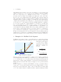
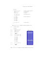
Download Getting Started with ADOL-C

2
A. Walther
ADOL-C provides a so-called tapeless forward mode, where the derivatives are
directly propagated together with the function values. In this case, no additionally sequential memory or data is required.
Applications that utilize ADOL-C can be found in many fields of science
and technology. This includes, e.g., fish stock assessment by the software package CASAL [4], computer-aided simulation of electronic circuits by fREEDA [5]
and the numerical simulation of optimal control problems by MUSCOD-II [6].
Currently, ADOL-C is further developed and maintained at the University of
Paderborn by a research group that is guided by Andrea Walther.
The key ingredient of automatic differentiation by overloading is the concept of an active variable. All variables that may be considered as differentiable
quantities at some time during the program execution must be of an active type.
Hence, all variables that lie on the way from the input variables, i.e., the independents, to the output variables, i.e., the dependents have to be redeclared to
be of the active type. For this purpose, ADOL-C introduces the new data type
adouble, whose real part is of the standard type double. In data flow terminology,
the set of active variable names must contain all its successors in the dependency
graph. Variables that do not depend on the independent variables but enter the
calculation, for example, as parameters, may remain one of the passive types
double, float, or int. There is no implicit type conversion from adouble to any of
these passive types; thus, failure to declare variables as active when they depend
on other active variables will result in a compile-time error message.
The derivative calculation is based on an internal function representation,
which is created during a separate so-called taping phase that starts with a call to
the routine trace on provided by ADOL-C and is finalized by calling the ADOLC routine trace off. All calculations involving active variables that occur between
the function calls trace on(tag,...) and trace off(...) are recorded on a sequential
data set called tape. Pairs of these function calls can appear anywhere in a
C++ program, but they must not overlap. The nonnegative integer argument
tag identifies the particular tape, i.e, internal function representation. Once, the
internal function representation is available, the drivers provided by ADOL-C
can be applied to compute the desired derivatives.
In some situations it may be desirable to calculate the derivatives of the function at arbitrary arguments by using a tape of the function evaluation at another
argument. Due to the avoidance of an additional taping process, this approach
can significantly reduce the overall run time. Therefore, the routines provided
by ADOL-C for the evaluation of derivatives can be used at arguments other
than the point at which the tape was generated, provided that all comparisons
involving adoubles yield the same result. The last condition implies that the
control flow is unaltered by the change of the independent variable values. The
return value of all ADOL-C drivers indicate this validity of the tape. If the user
finds the return value of an ADOL-C routine to be negative the taping process
simply has to be repeated by executing the active section again, since the tape
records only the operations that are executed during one particular evaluation
of the function.