Download Timer/Counter/ Analyzer

Timer/Counter/
Analyzer
PM6690
Operators Manual
PN 4822 872 20301
March 2007 - Seventh Edition
© 2005 Fluke Corporation. All rights reserved.
Printed in Sweden.
II
Table of Contents
GENERAL INFORMATION . . . . . . . . . . . . . VI
About this Manual . . . . . . . . . . . . . . . . . VI
Warranty . . . . . . . . . . . . . . . . . . . . . . . . VI
Declaration of Conformity . . . . . . . . . . . VI
Rear Panel . . . . . . . . . . . . . . . . . . . . . 2-5
Description of Keys . . . . . . . . . . . . . . . . . . 2-6
Power . . . . . . . . . . . . . . . . . . . . . . . . . 2-6
Select Function . . . . . . . . . . . . . . . . . . 2-6
Autoset/Preset. . . . . . . . . . . . . . . . . . . 2-6
Move Cursor . . . . . . . . . . . . . . . . . . . . 2-6
Display Contrast . . . . . . . . . . . . . . . . . 2-7
Enter . . . . . . . . . . . . . . . . . . . . . . . . . . 2-7
Save & Exit . . . . . . . . . . . . . . . . . . . . . 2-7
Don't Save & Exit. . . . . . . . . . . . . . . . . 2-7
Presentation Modes. . . . . . . . . . . . . . . 2-7
Entering Numeric Values . . . . . . . . . . . 2-8
Hard Menu Keys . . . . . . . . . . . . . . . . . 2-9
Default Settings . . . . . . . . . . . . . . . . . . . . 2-15
1 Preparation for Use
Preface . . . . . . . . . . . . . . . . . . . . . . . 1-2
Introduction . . . . . . . . . . . . . . . . . . . . . . . . 1-2
Powerful and Versatile Functions . . . . 1-2
No Mistakes. . . . . . . . . . . . . . . . . . . . . 1-3
Design Innovations . . . . . . . . . . . . . . . . . . 1-3
State of the Art Technology Gives
Durable Use . . . . . . . . . . . . . . . . . . . . 1-3
High Resolution . . . . . . . . . . . . . . . . . . 1-3
Remote Control . . . . . . . . . . . . . . . . . . . . . 1-4
Fast GPIB Bus. . . . . . . . . . . . . . . . . . . 1-4
3 Input Signal Conditioning
Safety . . . . . . . . . . . . . . . . . . . . . . . . 1-5
Input Amplifier . . . . . . . . . . . . . . . . . . . . . . 3-2
Impedance. . . . . . . . . . . . . . . . . . . . . . 3-2
Attenuation . . . . . . . . . . . . . . . . . . . . . 3-2
Coupling . . . . . . . . . . . . . . . . . . . . . . . 3-3
Filter . . . . . . . . . . . . . . . . . . . . . . . . . . 3-3
Man/Auto . . . . . . . . . . . . . . . . . . . . . . . 3-4
Trig . . . . . . . . . . . . . . . . . . . . . . . . . . . 3-5
How to Reduce or Ignore Noise and
Interference . . . . . . . . . . . . . . . . . . . . . . 3-6
Trigger Hysteresis . . . . . . . . . . . . . . . . 3-6
How to use Trigger Level Setting. . . . . 3-7
Introduction . . . . . . . . . . . . . . . . . . . . . . . . 1-5
Safety Precautions . . . . . . . . . . . . . . . . . . 1-5
Caution and Warning Statements . . . . 1-6
Symbols. . . . . . . . . . . . . . . . . . . . . . . . 1-6
If in Doubt about Safety . . . . . . . . . . . . 1-6
Unpacking . . . . . . . . . . . . . . . . . . . . 1-7
Check List . . . . . . . . . . . . . . . . . . . . . . . . . 1-7
Identification . . . . . . . . . . . . . . . . . . . . . . . 1-7
Installation . . . . . . . . . . . . . . . . . . . . . . . . . 1-7
Supply Voltage. . . . . . . . . . . . . . . . . . . 1-7
Grounding. . . . . . . . . . . . . . . . . . . . . . . . .
1-8
Orientation and Cooling . . . . . . . . . . . . 1-8
Fold-Down Support . . . . . . . . . . . . . . . 1-8
Rackmount Adapter. . . . . . . . . . . . . . . 1-9
4 Measuring Functions
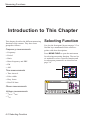
Introduction to This Chapter . . . . . 4-2
Selecting Function . . . . . . . . . . . . . . . . . . . 4-2
Frequency Measurements . . . . . . . 4-3
FREQ A, B. . . . . . . . . . . . . . . . . . . . . . . . . 4-3
FREQ C . . . . . . . . . . . . . . . . . . . . . . . . . . . 4-3
RATIO A/B, B/A, C/A, C/B . . . . . . . . . . . . . 4-4
BURST A, B, C . . . . . . . . . . . . . . . . . . . . . 4-4
Triggering . . . . . . . . . . . . . . . . . . . . . . 4-4
2 Using the Controls
Basic Controls . . . . . . . . . . . . . . . . . . . . . . 2-2
Secondary Controls . . . . . . . . . . . . . . . . . . 2-4
Connectors & Indicators . . . . . . . . . . . 2-4
III
Burst Measurements using Manual
Presetting . . . . . . . . . . . . . . . . . . . . . . 4-5
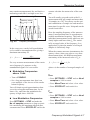
Frequency Modulated Signals . . . . . . . . . . 4-6
Carrier Wave Frequency f0 . . . . . . . . . 4-6
fmax . . . . . . . . . . . . . . . . . . . . . . . . . . . 4-7
fmin . . . . . . . . . . . . . . . . . . . . . . . . . . . . 4-7
Dfp-p . . . . . . . . . . . . . . . . . . . . . . . . . . . 4-8
Errors in fmax, fmin, and Dfp-p . . . . . . . . . 4-8
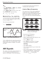
AM Signals . . . . . . . . . . . . . . . . . . . . . . . . 4-8
Carrier Wave Frequency . . . . . . . . . . . 4-8
Modulating Frequency . . . . . . . . . . . . . 4-9
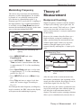
Theory of Measurement . . . . . . . . . . . . . . 4-9
Reciprocal Counting . . . . . . . . . . . . . . 4-9
Sample-Hold . . . . . . . . . . . . . . . . . . . 4-10
Time-Out . . . . . . . . . . . . . . . . . . . . . . 4-10
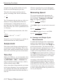
Measuring Speed . . . . . . . . . . . . . . . 4-10
PERIOD. . . . . . . . . . . . . . . . . . . . . . . . . . 4-12
Single A, B. . . . . . . . . . . . . . . . . . . . . 4-12
Average A, B, C. . . . . . . . . . . . . . . . . 4-12
Hold/Run & Restart . . . . . . . . . . . . . . . 5-2
Arming . . . . . . . . . . . . . . . . . . . . . . . . . 5-2
Start Arming. . . . . . . . . . . . . . . . . . . . . 5-3
Stop Arming. . . . . . . . . . . . . . . . . . . . . 5-3
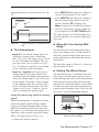
Controlling Measurement Timing . 5-4
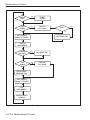
The Measurement Process . . . . . . . . . . . . 5-4
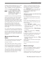
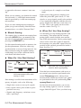
Resolution as Function of
Measurement Time . . . . . . . . . . . . . . . 5-4
Measurement Time and Rates . . . . . . 5-5
What is Arming? . . . . . . . . . . . . . . . . . 5-5
Arming Setup Time . . . . . . . . . . . . . . . . . . 5-9
Arming Examples . . . . . . . . . . . . . . . . . . . 5-9
Introduction to Arming Examples. . . . . 5-9
#1 Measuring the First Burst Pulse . . . 5-9
#2 Measuring the Second Burst Pulse5-11
#3 Measuring the Time Between
Burst Pulse #1 and #4 . . . . . . . . . . . . 5-12
#4 Profiling . . . . . . . . . . . . . . . . . . . . 5-13
6 Process
Time Measurements . . . . . . . . . . . 4-13
Introduction . . . . . . . . . . . . . . . . . . . . . . . . 6-2
Averaging . . . . . . . . . . . . . . . . . . . . . . 6-2
Mathematics . . . . . . . . . . . . . . . . . . . . . . . 6-2
Example: . . . . . . . . . . . . . . . . . . . . . . . 6-2
Statistics . . . . . . . . . . . . . . . . . . . . . . . . . . 6-3
Allan Deviation vs. Standard Deviation 6-3
Selecting Sampling Parameters . . . . . 6-3
Measuring Speed . . . . . . . . . . . . . . . . 6-4
Determining Long or Short Time
Instability . . . . . . . . . . . . . . . . . . . . . . . 6-4
Statistics and Mathematics . . . . . . . . . 6-5
Confidence Limits . . . . . . . . . . . . . . . . 6-5
Jitter Measurements . . . . . . . . . . . . . . 6-5
Limits . . . . . . . . . . . . . . . . . . . . . . . . . . . . . 6-6
Limit Behavior . . . . . . . . . . . . . . . . . . . 6-6
Limit Mode. . . . . . . . . . . . . . . . . . . . . . 6-7
Limits and Graphics. . . . . . . . . . . . . . . . . . 6-7
Introduction . . . . . . . . . . . . . . . . . . . . . . . 4-13
Triggering . . . . . . . . . . . . . . . . . . . . . 4-13
Time Interval . . . . . . . . . . . . . . . . . . . . . . 4-14
Time Interval A to B . . . . . . . . . . . . . . 4-14
Time Interval B to A . . . . . . . . . . . . . . 4-14
Time Interval A to A, B to B . . . . . . . . 4-14
Rise/Fall Time A/B. . . . . . . . . . . . . . . . . . 4-14
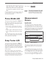
Pulse Width A/B . . . . . . . . . . . . . . . . . . . 4-15
Duty Factor A/B . . . . . . . . . . . . . . . . . . . . 4-15
Measurement Errors . . . . . . . . . . . . . . . . 4-15
Hysteresis . . . . . . . . . . . . . . . . . . . . . 4-15
Overdrive and Pulse Rounding . . . . . 4-16
Auto Trigger. . . . . . . . . . . . . . . . . . . . 4-16
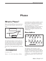
Phase . . . . . . . . . . . . . . . . . . . . . . . 4-17
What is Phase? . . . . . . . . . . . . . . . . . . . . 4-17
Resolution . . . . . . . . . . . . . . . . . . . . . . . . 4-17
Possible Errors . . . . . . . . . . . . . . . . . . . . 4-18
Inaccuracies . . . . . . . . . . . . . . . . . . . 4-18
7 Performance Check
General Information. . . . . . . . . . . . . . . . . . 7-2
Preparations . . . . . . . . . . . . . . . . . . . . . . . 7-2
Test Equipment . . . . . . . . . . . . . . . . . . . . . 7-2
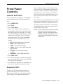
Front Panel Controls . . . . . . . . . . . . . . . . . 7-3
Internal Self-Tests . . . . . . . . . . . . . . . . 7-3
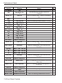
Keyboard Test . . . . . . . . . . . . . . . . . . . 7-3
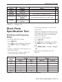
Short Form Specification Test . . . . . . . . . . 7-5
Sensitivity and Frequency Range . . . . 7-5
Voltage . . . . . . . . . . . . . . . . . . . . . . . . 7-6
Voltage . . . . . . . . . . . . . . . . . . . . . . 4-22
VMAX, VMIN, VPP . . . . . . . . . . . . . . . . . . . . 4-22
VRMS . . . . . . . . . . . . . . . . . . . . . . . . . . . . 4-23
5 Measurement Control
About This Chapter . . . . . . . . . . . . . . . . . . 5-2
Measurement Time . . . . . . . . . . . . . . . 5-2
Gate Indicator . . . . . . . . . . . . . . . . . . . 5-2
Single Measurements . . . . . . . . . . . . . 5-2
IV
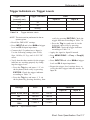
Trigger Indicators vs. Trigger Levels . . 7-7
Input Controls . . . . . . . . . . . . . . . . . . . 7-8
Reference Oscillators . . . . . . . . . . . . . 7-8
Resolution Test . . . . . . . . . . . . . . . . . . 7-9
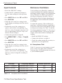
Rear Inputs/Outputs . . . . . . . . . . . . . . . . . 7-9
10 MHz OUT . . . . . . . . . . . . . . . . . . . . 7-9
EXT REF FREQ INPUT. . . . . . . . . . . . 7-9
EXT ARM INPUT. . . . . . . . . . . . . . . . . 7-9
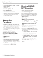
Measuring Functions . . . . . . . . . . . . . . . . 7-10
Check of HOLD OFF Function . . . . . . . . 7-10
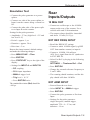
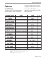
Options . . . . . . . . . . . . . . . . . . . . . . . . . . 7-11
Input C Check . . . . . . . . . . . . . . . . . . 7-11
Time Interval, Pulse Width, Rise/Fall
Time . . . . . . . . . . . . . . . . . . . . . . . . . 8-10
Frequency & Period. . . . . . . . . . . . . . 8-10
Frequency Ratio f1/f2 . . . . . . . . . . . . . 8-11
Phase . . . . . . . . . . . . . . . . . . . . . . . . 8-11
Duty Factor . . . . . . . . . . . . . . . . . . . . 8-11
Calibration . . . . . . . . . . . . . . . . . . . . . . . . 8-12
Definition of Terms. . . . . . . . . . . . . . . 8-12
General Specifications . . . . . . . . . . . . . . 8-12
Environmental Data . . . . . . . . . . . . . . 8-12
Power Requirements . . . . . . . . . . . . . 8-12
Dimensions & Weight . . . . . . . . . . . . 8-13
Ordering Information . . . . . . . . . . . . . . . . 8-13
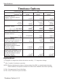
Timebase Options . . . . . . . . . . . . . . . . . . 8-14
Explanations . . . . . . . . . . . . . . . . . . . 8-14
8 Specifications
Introduction . . . . . . . . . . . . . . . . . . . . . . . . 8-2
Measurement Functions . . . . . . . . . . . . . . 8-2
Frequency A, B, C . . . . . . . . . . . . . . . . 8-2
Frequency Burst A, B, C . . . . . . . . . . . 8-2
Period A, B, C Average . . . . . . . . . . . . 8-2
Period A, B Single . . . . . . . . . . . . . . . . 8-3
Ratio A/B, B/A, C/A, C/B . . . . . . . . . . . 8-3
Time Interval A to B, B to A, A to A,
B to B. . . . . . . . . . . . . . . . . . . . . . . . . . 8-3
Pulse Width A, B . . . . . . . . . . . . . . . . . 8-3
Rise and Fall Time A, B . . . . . . . . . . . . 8-3
Phase A Rel. B, B Rel. A . . . . . . . . . . . 8-4
Duty Factor A, B . . . . . . . . . . . . . . . . . 8-4
Vmax, Vmin, Vp-p A, B . . . . . . . . . . . . . . . 8-4
Timestamping A, B, C . . . . . . . . . . . . . 8-5
Auto Set / Manual Set . . . . . . . . . . . . . 8-5
Input and Output Specifications . . . . . . . . 8-5
Inputs A and B . . . . . . . . . . . . . . . . . . . 8-5
Input C (PM6690/6xx) . . . . . . . . . . . . . 8-6
Input C (PM6690/7xx) . . . . . . . . . . . . . 8-6
Rear Panel Inputs & Outputs . . . . . . . . 8-6
Auxiliary Functions . . . . . . . . . . . . . . . . . . 8-7
Trigger Hold-Off . . . . . . . . . . . . . . . . . . 8-7
External Start/Stop Arming . . . . . . . . . 8-7
Statistics . . . . . . . . . . . . . . . . . . . . . . . 8-7
Mathematics . . . . . . . . . . . . . . . . . . . . 8-7
Other Functions . . . . . . . . . . . . . . . . . . 8-7
Display. . . . . . . . . . . . . . . . . . . . . . . . . 8-8
GPIB Interface . . . . . . . . . . . . . . . . . . . 8-8
USB Interface . . . . . . . . . . . . . . . . . . . 8-8
TimeView™ . . . . . . . . . . . . . . . . . . . . . 8-8
Measurement Uncertainties . . . . . . . . . . 8-10
Random Uncertainties (1s) . . . . . . . . 8-10
Systematic Uncertainties . . . . . . . . . . 8-10
Total Uncertainty (2s) . . . . . . . . . . . . 8-10
9 Index
10 Service
Sales and Service office . . . . . . . . . . . . . 10-2
V
GENERAL INFORMATION
About this Manual
This manual contains directions for use that apply to the Timer/Counter/Analyzer PM6690.
In order to simplify the references, the PM6690 is further referred to throughout this manual
as the '90'.
Warranty
The Warranty Statement is part of the Getting Started Manual that is included with the shipment.
Declaration of Conformity
The complete text with formal statements concerning product identification, manufacturer and
standards used for type testing is available on request.
VI
Chapter 1
Preparation for Use
Preparation for Use
Preface
Introduction
Congratulations on your choice of instrument.
It will serve you well for many years to come.
Your Timer/Counter/Analyzer is designed to
bring you a new dimension to bench-top and
system counting. It offers significantly increased performance compared to traditional
Timer/Counters. The PM6690 offers the following advantages:
– 12 digits of frequency resolution per second and 100 ps resolution, as a result of
high-resolution interpolating reciprocal
counting.
– RF prescaler options with upper frequency
limit of 3 GHz or 8 GHz.
– Integrated high performance GPIB interface using SCPI commands.
– A fast USB interface that replaces the traditional but slower RS-232 serial interface.
– Timestamping; the counter records exactly
when a measurement is made.
– A high measurement rate of up to
250 k readings/s to internal memory.
– Optional oven-controlled timebase
oscillators.
1-2 Preface
Powerful and Versatile
Functions
A unique performance feature in your new instrument is the comprehensive arming possibilities, which allow you to characterize virtually any type of complex signal concerning
frequency and time.
For instance, you can insert a delay between
the external arming condition and the actual
arming of the counter. Read more about Arming in Chapter 5, “Measurement Control”.
In addition to the traditional measurement
functions of a timer/counter, these instruments
have a multitude of other functions such as
phase, duty factor, rise/fall-time and peak
voltage. The counter can perform all
measurement functions on both main inputs
(A & B). Most measurement functions can be
armed, either via one of the main inputs or via
a separate arming channel (E).
By using the built-in mathematics and statistics functions, the instrument can process the
measurement results on your benchtop, without the need for a controller. Math functions
include inversion, scaling and offset. Statistics
functions include Max, Min and Mean as well
Preparation for Use
as Standard and Allan Deviation on sample
sizes up to 2*109.
Design Innovations
No Mistakes
State of the Art Technology
Gives Durable Use
You will soon find that your instrument is
more or less self-explanatory with an intuitive
user interface. A menu tree with few levels
makes the timer/counter easy to operate. The
large backlit graphic LCD is the center of information and can show you several signal parameters at the same time as well as setting
status and operator messages.
Statistics based on measurement samples can
easily be presented as histograms or trend
plots in addition to standard numerical measurement results like max, min, mean and
standard deviation.
The AUTO function triggers automatically on
any input waveform. A bus-learn mode simplifies GPIB programming. With bus-learn
mode, manual counter settings can be transferred to the controller for later reprogramming. There is no need to learn code and syntax for each individual counter setting if you
are an occasional bus user.
These counters are designed for quality and
durability. The design is highly integrated.
The digital counting circuitry consists of just
one custom-developed FPGA and a 32-bit
microcontroller. The high integration and low
component count reduces power consumption
and results in an MTBF of 30,000 hours.
Modern surface-mount technology ensures
high production quality. A rugged mechanical
construction, including a metal cabinet that
withstands mechanical shocks and protects
against EMI, is also a valuable feature.
High Resolution
The use of reciprocal interpolating counting
in this new counter results in excellent relative
resolution: 12 digits/s for all frequencies.
The measurement is synchronized with the input cycles instead of the timebase. Simultaneously with the normal “digital” counting,
the counter makes analog measurements of
the time between the start/stop trigger events
and the next following clock pulse. This is
done in four identical circuits by charging an
integrating capacitor with a constant current,
starting at the trigger event. Charging is
stopped at the leading edge of the first following clock pulse. The stored charge in the integrating capacitor represents the time difference between the start trigger event and the
leading edge of the first following clock pulse.
A similar charge integration is made for the
stop trigger event.
When the “digital” part of the measurement is
ready, the stored charges in the capacitors are
Preface 1-3
Preparation for Use
measured by means of Analog/Digital
Converters.
The counter’s microprocessor calculates the
result after completing all measurements, i.e.
the digital time measurement and the analog
interpolation measurements.
The result is that the basic “digital resolution”
of ± 1 clock pulse (10 ns) is reduced to 100 ps
for the '90'.
Since the measurement is synchronized with
the input signal, the resolution for frequency
measurements is very high and independent of
frequency.
The counters have 14 display digits to ensure
that the display itself does not restrict the resolution.
Fast GPIB Bus
These counters are not only extremely powerful and versatile bench-top instruments, they
also feature extraordinary bus properties.
The bus transfer rate is up to 2000 triggered
measurements/s. Array measurements to the
internal memory can reach 250 k measurements/s.
This very high measurement rate makes new
measurements possible. For example, you can
perform jitter analysis on several tens of thousands of pulse width measurements and capture them in a second.
An extensive programming manual helps you
understand SCPI and counter programming.
This instrument is programmable via two interfaces, GPIB and USB.
The counter is easy to use in GPIB environments. A built-in bus-learn mode enables you
to make all counter settings manually and
transfer them to the controller. The response
can later be used to reprogram the counter to
the same settings. This eliminates the need for
the occasional user to learn all individual programming codes.
The GPIB interface offers full general functionality and compliance with the latest standards in use, the IEEE 488.2 1987 for HW and
the SCPI 1999 for SW.
Complete (manually set) counter settings can
also be stored in 20 internal memory locations
and can easily be recalled on a later occasion.
Ten of them can be user protected.
Remote Control
In addition to this 'native' mode of operation
there is also a second mode that emulates the
Agilent 53131/132 command set for easy exchange of instruments in operational ATE
systems.
The USB interface is mainly intended for the
lab environment in conjunction with the optional TimeView™ analysis software. The
communication protocol is a proprietary version of SCPI.
1-4 Preface
Preparation for Use
Safety
Introduction
Safety Precautions
Even though we know that you are eager to
get going, we urge you to take a few minutes
to read through this part of the introductory
chapter carefully before plugging the line connector into the wall outlet.
All equipment that can be connected to line
power is a potential danger to life. Handling
restrictions imposed on such equipment
should be observed.
This instrument has been designed and tested
for Measurement Category I, Pollution Degree
2, in accordance with EN/IEC 61010-1:2001
and CAN/CSA-C22.2 No. 61010-1-04 (including approval). It has been supplied in a
safe condition.
Study this manual thoroughly to acquire adequate knowledge of the instrument, especially
the section on Safety Precautions hereafter
and the section on Installation on page 1-7.
To ensure the correct and safe operation of the
instrument, it is essential that you follow generally accepted safety procedures in addition
to the safety precautions specified in this manual.
The instrument is designed to be used by
trained personnel only. Removing the cover
for repair, maintenance, and adjustment of the
instrument must be done by qualified personnel who are aware of the hazards involved.
The warranty commitments are rendered
void if unauthorized access to the interior
of the instrument has taken place during
the given warranty period.
Safety 1-5
Preparation for Use
Caution and Warning
Statements
CAUTION: Shows where incorrect
procedures can cause damage to,
or destruction of equipment or
other property.
WARNING: Shows a potential danger
that requires correct procedures or
practices to prevent personal injury.
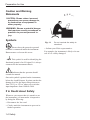
Symbols
Fig. 1-1
Shows where the protective ground
terminal is connected inside the instrument.
Never remove or loosen this screw.
This symbol is used for identifying the
functional ground of an I/O signal. It is always
connected to the instrument chassis.
Indicates that the operator should
consult the manual.
One such symbol is printed on the instrument,
below the A and B inputs. It points out that the
damage level for the input voltage decreases
from 350 Vp to 12Vrms when you switch the
input impedance from 1 MW to 50 W.
If in Doubt about Safety
Whenever you suspect that it is unsafe to use
the instrument, you must make it inoperative
by doing the following:
– Disconnect the line cord
– Clearly mark the instrument to prevent its
further operation
1-6 Safety
Do not overlook the safety instructions!
– Inform your Fluke representative.
For example, the instrument is likely to be unsafe if it is visibly damaged.
Preparation for Use
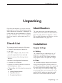
Unpacking
Check that the shipment is complete and that
no damage has occurred during transportation.
If the contents are incomplete or damaged, file
a claim with the carrier immediately. Also notify your local Fluke sales or service organization in case repair or replacement may be required.
Check List
The shipment should contain the following:
– Counter/Timer/Analyzer, Model 90
– Line cord
– N-to-BNC Adapter (only if one of the
prescaler options has been ordered)
– Printed version of the Getting Started
Manual
– Brochure with Important Information
– Certificate of Calibration
– Options you ordered should be installed.
See Identification below.
– CD including the following documentation
in PDF:
•
•
•
Getting Started Manual
Operators Manual
Identification
The type plate on the rear panel shows type
number and serial number. See illustration on
page 2-5. In the menu User Options - About
you can find information on firmware version
and calibration date. See page 2-12.
Installation
Supply Voltage
n Setting
The Counter may be connected to any AC
supply with a voltage rating of 90 to 265
Vrms , 45 to 440 Hz. The counter automatically adjusts itself to the input line voltage.
n Fuse
The secondary supply voltages are electronically protected against overload or short circuit. The primary line voltage side is protected
by a fuse located on the power supply unit.
The fuse rating covers the full voltage range.
Consequently there is no need for the user to
replace the fuse under any operating conditions, nor is it accessible from the outside.
Programming Manual
Unpacking 1-7
Preparation for Use
CAUTION: If this fuse is blown, it is
likely that the power supply is
badly damaged. Do not replace the
fuse. Send the counter to the local
Service Center.
Removing the cover for repair, maintenance
and adjustment must be done by qualified and
trained personnel only, who are fully aware of
the hazards involved.
Orientation and Cooling
The counter can be operated in any position
desired. Make sure that the air flow through
the ventilation slots at the top, and side panels
is not obstructed. Leave 5 centimeters (2
inches) of space around the counter.
Fold-Down Support
The warranty commitments are rendered
void if unauthorized access to the interior
of the instrument has taken place during
the given warranty period.
Fig. 1-2
Fold-down support for comfortable bench-top use.
Grounding
Grounding faults in the line voltage supply
will make any instrument connected to it dangerous. Before connecting any unit to the
power line, you must make sure that the protective ground functions correctly. Only then
can a unit be connected to the power line and
only by using a three-wire line cord. No other
method of grounding is permitted. Extension
cords must always have a protective ground
conductor.
CAUTION: If a unit is moved from a
cold to a warm environment, condensation may cause a shock
hazard. Ensure, therefore, that the
grounding requirements are strictly
met.
WARNING: Never interrupt the
grounding cord. Any interruption of
the protective ground connection
inside or outside the instrument or
disconnection of the protective
ground terminal is likely to make
the instrument dangerous.
1-8 Unpacking
For bench-top use, a fold-down support is
available for use underneath the counter. This
support can also be used as a handle to carry
the instrument.
Preparation for Use
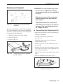
Rackmount Adapter
WARNING: Do not perform any internal service or adjustment of this
instrument unless you are qualified
to do so.
Before you remove the cover, disconnect mains cord and wait for
one minute.
Fig. 1-3
Dimensions for rackmounting
hardware.
If you have ordered a 19-inch rack-mount kit
for your instrument, it has to be assembled after delivery of the instrument. The rackmount
kit consists of the following:
– 2 brackets, (short, left; long, right)
– 4 screws, M5 x 8
– 4 screws, M6 x 8
Capacitors inside the instrument
can hold their charge even if the instrument has been separated from
all voltage sources.
n Assembling the Rackmount Kit
– Make sure the power cord is disconnected
from the instrument.
– Turn the instrument upside down.
See Fig. 1-5.
– Undo the two screws (A) and remove
them from the cover.
– Remove the rear feet by undoing the two
screws (B).
– Remove the four decorative plugs (C) that
cover the screw holes on the right and left
side of the front panel.
– Grip the front panel and gently push at the
Fig. 1-4
Fitting the rack mount brackets
on the counter.
rear.
– Pull the instrument out of the cover.
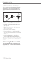
Fig. 1-5
Remove the screws and push the
counter out of the cover.
Unpacking 1-9
Preparation for Use
– Remove the four feet from the cover.
Use a screwdriver as shown in the following
illustration or a pair of pliers to remove the
springs holding each foot, then push out the
feet.
Fig. 1-6
Removing feet from the cover.
– Push the instrument back into the cover.
See Fig. 1-5.
– Mount the two rear feet with the screws
(B) to the rear panel.
– Put the two screws (A) back.
– Fasten the brackets at the left and right
side with the screws included as illustrated
in Fig. 1-3.
– Fasten the instrument in the rack via
screws in the four rack-mounting holes
The long bracket has an opening so that cables
for Input A, B, and C can be routed inside the
rack.
n Reversing the Rackmount Kit
The instrument may also be mounted to the
right in the rack. To do so, swap the position
of the two brackets.
1-10 Unpacking
Chapter 2
Using the Controls
Using the Controls
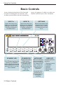
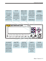
Basic Controls
A more elaborate description of the front and
rear panels including the user interface with
its menu system follows after this introductory
survey, the purpose of which is to make you
familiar with the layout of the instrument.
INPUT A
INPUT B
SETTINGS
Opens the menu from
which you can adjust all
settings for Input A like
Coupling, Impedance
and Attenuation.
Opens the menu from
which you can adjust all
settings for Input B like
Coupling, Impedance
and Attenuation.
Select measurement parameters such as measurement time, number
of measurements, and
so on.
STANDBY LED
The LED lights up when the
counter is in STANDBY
mode, indicating that power
is still applied to an internal
optional OCXO, if one has
been installed.
2-2 Basic Controls
STANDBY/ON
MATH/LIMIT
Toggling secondary
power switch.
Pressing this button
in standby mode
turns the counter
ON and restores the
settings as they
were at
power-down.
Menu for selecting
one of a set of formulas for modifying
the measurement
result. Three constants can be entered from the
keyboard.
Numerical limits
can also be entered for status reporting and
recording
USER OPT.
Controls the following items:
1. Settings memory
2. Calibration
3. Interface
4. Self-test
5. Blank digits
6. About
Using the Controls
STAT/PLOT
VALUE
MEAS FUNC
AUTO SET
Menu tree for
selecting measurement function.
Adjusts input
trigger voltages
automatically to
the optimum levels for the chosen measurement function.
CURSOR
CONTROL
Enters one of
three statistics
presentation
modes.
Switching between the modes
is done by
toggling the key.
Enters the normal numerical
presentation
mode with one
main parameter
and a number of
auxiliary parameters.
HOLD/RUN
RESTART
EXIT/OK
CANCEL
ENTER
Toggles between
HOLD (one-shot)
mode and RUN
(continuous)
mode. Freezes
the result after
completion of a
measurement if
HOLD is active.
Initiates one
new measurement if HOLD is
active.
Confirms menu
selections and
moves up one
level in the menu
tree.
Moves up one
menu level without confirming
selections made.
Confirms menu
selections without leaving the
menu level.
You can use the
seven softkeys
below the display for confirmation.
Double-click for
default settings.
The cursor
position, marked
by text inversion
on the display,
can be moved in
four directions.
Exits REMOTE
mode if not
LOCAL
LOCKOUT.
Basic Controls 2-3
Using the Controls
Secondary Controls
Connectors & Indicators
GRAPHIC DISPLAY
SOFTKEYS
320 x 97 pixels LCD with backlight for showing measurement results in numerical as well
as graphical format. The display is also the
center of the dynamic user interface, comprising menu trees, indicators and information
boxes.
The function of these seven keys is menu dependent. Actual function is indicated on the
LCD.
Depressing a softkey is often a faster alternative to moving the cursor to the desired position and then pressing OK.
RF INPUT
TRIGGER INDICATORS
GATE INDICATOR
Blinking LED indicates correct
triggering.
A pending measurement
causes the
LED to light up.
MAIN INPUTS
The two identical DC
coupled channels A &
B are used for all
types of measurements, either one at a
time or both together.
NUMERIC INPUT KEYS
Sometimes you may want to enter numeric values like the
constants and limits asked for when you are utilizing the
postprocessing features in MATH/LIMIT mode. These
twelve keys are to be used for this purpose.
2-4 Secondary Controls
(Optional Input C)
A number of RF
prescalers are
available, covering
different frequency
ranges. These units
are fully automatic
and no controls affect the performance. The Type
N connector is fitted only if a
prescaler is
installed.
Using the Controls
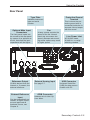
Rear Panel
Protective Ground
Terminal
Type Plate
Indicates instrument
type and serial
number.
Optional Main Input
Connectors
Fan
A temp. sensor controls the
speed of the fan. Normal
bench-top use means low
speed, whereas rack-mounting and/or options may result
in higher speed.
The front panel inputs can
be moved to the rear panel
by means of an optional cable kit. Note that the input
capacitance will be higher.
!
!
This is where the protective ground wire is
connected inside the instrument. Never tamper
with this screw!
Line Power Inlet
AC 90-265 VRMS,
45-440 Hz, no range
switching needed.
!
191125
Reference Output
10 MHz derived from the
internal or, if present, the
external reference.
External Reference
Input
Can be automatically selected if a signal is present and approved as
timebase source, see
Chapter 9.
External Arming Input
See page 5-7.
USB Connector
Universal Serial Bus
(USB) for data communication with PC.
GPIB Connector
Address set via User Options Menu.
Secondary Controls 2-5
Using the Controls
Description of Keys
Power
The ON/OFF key is a toggling secondary
power switch. Part of the instrument is always
ON as long as power is applied, and this
standby condition is indicated by a red LED
above the key. This indicator is consequently
not lit while the instrument is in operation.
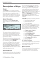
Select Function
This hard key is marked MEAS FUNC.
When you depress it, the menu below will
open.
nel, you will most probably get a measurement result. The AUTOSET system ensures
that the trigger levels are set optimally for
each combination of measurement function
and input signal amplitude, provided relatively normal signal waveforms are applied. If
Manual Trigger has been selected before
pressing the AUTOSET key, the system will
make the necessary adjustments once
(Auto Once) and then return to its inactive
condition.
AUTOSET performs the following functions:
•
•
•
Set automatic trigger levels
Switch attenuators to 1x
Turn on the display
By depressing this key twice within two seconds, you will enter the Preset mode, and a
more extensive automatic setting will take
place. In addition to the functions above, the
following functions will be performed:
Fig. 2-1
Select measurement function.
The current selection is indicated by text inversion that is also indicating the cursor position. Select the measurement function you
want by depressing the corresponding softkey
right below the display.
Alternatively you can move the cursor to the
wanted position with the RIGHT/LEFT arrow
keys. Confirm by pressing ENTER.
A new menu will appear where the contents
depend on the function. If you for instance
have selected Frequency, you can then select
between Frequency, Frequency Ratio and
Frequency Burst. Finally you have to decide
which input channel(s) to use.
Autoset/Preset
By depressing this key once after selecting the
wanted measurement function and input chan-
2-6 Description of Keys
•
•
•
•
•
•
•
Set Meas Time to 200 ms
Switch off Hold-Off
Set HOLD/RUN to RUN
Switch off MATH/LIM
Switch off Analog and Digital Filters
Set Timebase Ref to Internal
Switch off Arming
n Default Settings
An even more comprehensive preset function
can be performed by recalling the factory default settings. See page 2-13.
Move Cursor
There are four arrow keys for moving the cursor, normally marked by text inversion,
around the menu trees in two dimensions.
Using the Controls
Display Contrast
When no cursor is visible (no active menu selected), the UP/DOWN arrows are used for
adjusting the LCD display contrast ratio.
full resolution together with a number of auxiliary parameters in small characters with limited resolution.
Enter
The key marked ENTER enables you to confirm a choice without leaving your menu position.
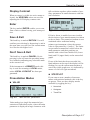
Save & Exit
This hard key is marked EXIT/OK. You will
confirm your selection by depressing it, and at
the same time you will leave the current menu
level for the next higher level.
Don't Save & Exit
This hard key is marked CANCEL. By depressing it you will enter the preceding menu
level without confirming any selections made
at the current level.
If the instrument is in REMOTE mode, this
key is used for returning to LOCAL mode,
unless LOCAL LOCKOUT has been programmed.
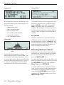
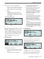
Presentation Modes
n VALUE
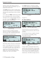
Fig. 2-3
If Limits Alarm is enabled you can visualize
the deviation of your measurements in relation
to the set limits. The numerical readout is now
combined with a traditional analog
pointer-type instrument, where the current
value is represented by a "smiley". The limits
are presented as numerical values below the
main parameter, and their positions are
marked with vertical bars labelled LL (lower
limit) and UL (upper limit) on the autoscaled
graph.
If one of the limits has been exceeded, the
limit indicator at the top of the display will be
flashing. In case the current measurement is
out of the visible graph area, it is indicated by
means of a left or a right arrowhead.
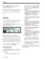
n STAT/PLOT
If you want to treat a number of measurements with statistical methods, this is the key
to operate. There are three display modes
available by toggling the key:
•
•
•
Fig. 2-2
Limits presentation.
Numerical
Histogram
Trend Plot
Main and aux. parameters.
Value mode gives single line numerical presentation of individual results, where the main
parameter is displayed in large characters with
Description of Keys 2-7
Using the Controls
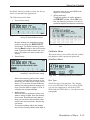
Numerical
Fig. 2-4
Trend Plot
Statistics presented numerically.
In this mode the statistical information is displayed as numerical data containing the following elements:
•
•
•
•
•
•
Mean: mean value
Max: maximum value
Min: minimum value
P-P: peak-to-peak deviation
Adev: Allan deviation
Std: Standard deviation
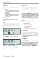
Histogram
Fig. 2-5
Statistics presented as a histogram.
The bins in the histogram are always
autoscaled based on the measured data. Limits, if enabled, and center of graph are shown
as vertical dotted lines. Data outside the limits
are not used for autoscaling but are replaced
by an arrow indicating the direction where
non-displayed values have been recorded.
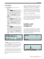
Fig. 2-6
Running trend plot.
This mode is used for observing periodic fluctuations or possible trends. Each plot terminates (if HOLD is activated) or restarts (if
RUN is activated) after the set number of
samples. The trend plot is always autoscaled
based on the measured data, starting with 0 at
restart. Limits are shown as horizontal lines if
enabled.
n Remote
When the instrument is controlled from the
GPIB bus, and the remote line is asserted, the
presentation mode changes to Remote, indicated by the label Remote on the display. The
main measurement result and the input settings are displayed in this mode.
Entering Numeric Values
Sometimes you may want to enter constants
and limits in a value input menu, for instance
one of those that you can reach when you
press the MATH/LIMIT key.
You may also want to select a value that is not
in the list of fixed values available by pressing
the UP/DOWN arrow keys. One example is
Meas Time under SETTINGS.
A similar situation arises when the desired
value is too far away to reach conveniently by
incrementing or decrementing the original
value with the UP/DOWN arrow keys. One
example is the Trig Lvl setting as part of the
INPUT A (B) settings.
2-8 Description of Keys
Using the Controls
Whenever it is possible to enter numeric values, the keys marked with 0-9; . (decimal
point) and ± (stands for Change Sign) take on
their alternative numeric meaning.
It is often convenient to enter values using the
scientific format. For that purpose, the
rightmost softkey is marked EE (stands for
Enter Exponent), making it easy to switch between the mantissa and the exponent.
Press EXIT/OK to store the new value or
CANCEL to keep the old one.
•
•
•
•
Impedance: 50 W or 1 MW
•
Filter:3 On or Of
Attenuation: 1x or 10x
Trigger:1 Manual or Auto
Trigger Level:2 numerical input via front
panel keyboard. If Auto Trigger is active,
you can change the default trigger level
manually as a percentage of the
amplitude.
Notes: 1
Always Auto when measuring
2
The absolute level can either be
adjusted using the up/down
arrow keys or by pressing
ENTER to reach the numerical
input menu.
Pressing the corresponding
softkey or ENTER opens the
Filter Settings menu. See Fig.
2-8. You can select a fixed
100 kHz analog filter or an
adjustable digital filter. The
equivalent cutoff frequency is
set via the value input menu
that opens if you select Digital
LP Frequency from the menu.
risetime or falltime
Hard Menu Keys
These keys are mainly used for opening fixed
menus from which further selections can be
made by means of the softkeys or the cursor/select keys.
3
n Input A (B)
Fig. 2-7
Input settings menu.
By depressing this key, the bottom part of the
display will show the settings for Input A (B).
The active settings are in bold characters and
can be changed by depressing the corresponding softkey below the display. You can also
move the cursor, indicated by text inversion,
to the desired position with the RIGHT/LEFT
arrow keys and then change the active setting
with the ENTER key.
Fig. 2-8
Selecting analog or digital filter.
n Input B
The settings under Input B are equal to those
under Input A.
The selections that can be made using this
menu are:
•
Trigger Slope: positive or negative, indicated by corresponding symbols
•
Coupling: AC or DC
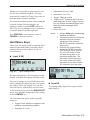
Description of Keys 2-9
Using the Controls
n Settings
Fig. 2-9
The main settings menu.
This key accesses a host of menus that affect
the measurement. The figure above is valid after changing the default measuring time to
10 ms.
Meas Time
Arm
Fig. 2-12
Setting arming conditions.
Arming is the general term used for the means
to control the actual start/stop of a measurement. The normal free-running mode is inhibited and triggering takes place when certain
pretrigger conditions are fulfilled.
The signal or signals used for initiating the
arming can be applied to three channels (A, B,
E), and the start channel can be different from
the stop channel. All conditions can be set via
the menu below.
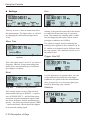
Fig. 2-10
Submenu for entering measuring time.
Trigger Hold-Off
This value input menu is active if you select a
frequency function. Longer measuring time
means fewer measurements per second and
gives higher resolution.
Fig. 2-13
Burst
The trigger hold-off submenu.
A value input menu is opened where you can
set the delay during which the stop trigger
conditions are ignored after the measurement
start. A typical use is to clean up signals generated by bouncing relay contacts.
Fig. 2-11
Entering burst parameters.
This settings menu is active if the selected
measurement function is BURST – a special
case of FREQUENCY – and facilitates measurements on pulse-modulated signals. Both
the carrier frequency and the modulating frequency – the pulse repetition frequency (PRF)
– can be measured, often without the support
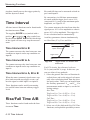
of an external arming signal.
2-10 Description of Keys
Statistics
Fig. 2-14
Entering statistics parameters.
Using the Controls
timestamping which measurement
channel precedes the other.
In this menu you can do the following:
•
Set the number of samples used for calculation of various statistical measures.
•
Set the number of bins in the histogram
view.
•
Pacing
The delay between measurements,
called pacing, can be set to ON or OFF,
and the time can be set within the range
2 ms – 1000 s.
•
Smart Frequency (valid only if the selected measurement function is Frequency or Period Average)
By means of continuous timestamping
and regression analysis, the resolution
is increased for measuring times between 0.2 s and 100 s.
•
Auto Trig Low Freq
In a value input menu you can set the
lower frequency limit for automatic triggering and voltage measurements
within the range 1 Hz – 100 kHz. A
higher limit means faster settling time
and consequently faster measurements.
•
Timeout
From this submenu you can activate/deactivate the timeout function and set the
maximum time the instrument will wait
for a pending measurement to finish before outputting a zero result. The range
is 10 ms to 1000 s.
Timebase Reference
Fig. 2-15
Selecting timebase reference
source.
Here you can decide if the counter is to use an
Internal or an External timebase. A third alternative is Auto. Then the external timebase
will be selected if a valid signal is present at
the reference input. The EXT REF indicator at
the upper right corner of the display shows
that the instrument is using an external
timebase reference.
n Math/Limit
Fig. 2-17
Miscellaneous
Selecting 'Math' or 'Limits' parameters.
You enter a menu where you can choose between inputting data for the Mathematics or
the Limits postprocessing unit.
Fig. 2-16
The 'Misc' submenu.
The options in this menu are:
•
Smart Time Interval (valid only if the selected measurement function is Time Interval)
The counter decides by means of
Fig. 2-18
The 'Math' submenu.
The Math branch is used for modifying the
measurement result mathematically before
presentation on the display. Thus you can
Description of Keys 2-11
Using the Controls
make the counter show directly what you
want without tedious recalculations, e.g. revolutions/min instead of Hz.
The Limit submenu is treated in a similar
way, and its features are explored beginning
The Limits branch is used for setting numerical limits and selecting the way the instrument
will report the measurement results in relation
to them.
Let us explore the Math submenu by pressing
the corresponding softkey below the display.
The display tells you that the Math function is
not active, so press the Math Off key once to
open the formula selection menu.
Fig. 2-19
Selecting 'Math' formula for
postprocessing.
Select one of the five different formulas,
where K, L and M are constants that the user
can set to any value. X stands for the current
non-modified measurement result.
Fig. 2-21
Entering numeric values for
constants.
on page 6-6.
n User Options
Fig. 2-22
The User Options menu.
From this menu you can reach a number of
submenus that do not directly affect the measurement.
You can choose between a number of modes
by pressing the corresponding softkey.
Save/Recall Menu
Fig. 2-20
Selecting formula constants.
Each of the softkeys below the constant labels
opens a value input menu like the one below.
Use the numeric input keys to enter the mantissa and the exponent, and use the EE key to
toggle between the input fields. The key
marked X0 is used for entering the display
reading as the value of the constant.
2-12 Description of Keys
Fig. 2-23
The memory management
menu.
Twenty complete front panel setups can be
stored in non-volatile memory. Access to the
first ten memory positions is prohibited when
Setup Protect is ON. Switching OFF Setup
Protect releases all ten memory positions simultaneously. The different setups can be in-
Using the Controls
dividually labeled to make it easier for the operator to remember the application.
The following can be done:
•
Save current setup
Fig. 2-24
•
Setup protection
Toggle the softkey to switch between
the ON/OFF modes. When ON is active, the memory positions 1-10 are all
protected against accidental overwriting.
Selecting memory position for
saving a measurement setup.
Browse through the available memory
positions by using the RIGHT/LEFT
arrow keys. For faster browsing, press
the key Next to skip to the next memory
bank. Press the softkey below the number (1-20) where you want to save the
setting.
•
the same way as you write SMS messages on a cell phone.
Recall setup
Fig. 2-26
Entering alphanumeric characters.
Calibrate Menu
This menu entry is accessible only for calibration purposes and is password-protected.
Interface Menu
Fig. 2-25
Selecting memory position for
recalling a measurement setup.
Fig. 2-27
Select the memory position from which
you want to retrieve the contents in the
same way as under Save current setup
above. You can also choose Default to
restore the preprogrammed factory settings. See the table on page 2-15 for a
complete list of these settings.
•
Modify labels
Select a memory position to which you
want to assign a label. See the descriptions under Save/Recall setup above.
Now you can enter alphanumeric characters from the front panel. See the figure below.
The seven softkeys below the display
are used for entering letters and digits in
Selecting active bus interface.
Bus Type
Select the active bus interface. The alternatives are GPIB and USB. If you select GPIB,
you are also supposed to select the GPIB
Mode and the GPIB Address. See the next two
paragraphs.
Description of Keys 2-13
Using the Controls
GPIB Mode
Blank Digits
There are two command systems to choose
from.
Jittery measurement results can be made easier for an operator to read by masking one or
more of the LSDs on the display.
•
•
Native
The SCPI command set used in this mode
fully exploits all the features of this instrument series.
Compatible
The SCPI command set used in this mode is
adapted to be compatible with Agilent
53131/132/181.
GPIB Address
Value input menu for setting the GPIB address.
Place the cursor at the submenu Digits Blank
and increment/decrement the number by
means of the UP/DOWN arrow keys, or press
the soft key beneath the submenu and enter
the desired number between 0 and 13 from the
keyboard. The blanked digits will be represented by dashes on the display. The default
value for the number of blanked digits is 0.
About
Here you can find information on:
Test
A general self-test is always performed every
time you power-up the instrument, but you
can order a specific test from this menu at any
time.
•
•
calibration date
firmware versions for:
«
«
•
basic instrument
interfaces
optional factory-installed hardware
n Hold/Run
Fig. 2-28
Self-test menu.
Press Test Mode to open the menu with
available choices.
Fig. 2-29
Selecting a specific test.
Select one of them and press Start Test to
run it.
2-14 Description of Keys
This key serves the purpose of manual arming. A pending measurement will be finished
and the result will remain on the display until
a new measurement is triggered by pressing
the RESTART key.
n Restart
Often this key is operated in conjunction with
the HOLD/RUN key (see above), but it can
also be used in free-running mode, especially
when long measuring times are being used,
e.g. to initiate a new measurement after a
change in the input signal. RESTART will
not affect any front panel settings.
Using the Controls
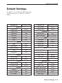
Default Settings
See page 2-13 to see how the following preprogrammed settings are recalled by a few keystrokes.
PARAMETER
VALUE/SETTING
Input A & B
PARAMETER
VALUE/SETTING
Pacing State
OFF
Pacing Time
20 ms
Trigger Level
AUTO
Trigger Slope
POS (A), NEG (B)
Impedance
1 MW
Mathematics
OFF
Attenuator
1x
Math Constants
K=1, L=0, M=1
Coupling
AC
Filter
OFF
Arming
Mathematics
Limits
Limit State
OFF
Limit Mode
ABOVE
0
Start
OFF
Lower Limit
Upper Limit
Start Slope
POS
Start Arm Delay
0
Stop
OFF
Sync Delay
400 ms
Stop Slope
POS
Start Delay
0
Hold-Off
Hold-Off State
OFF
Hold-Off Time
200 ms
Time-Out
0
Burst
Meas. Time
200 ms
Freq. Limit
300 MHz
Miscellaneous
Time-Out State
OFF
Function
FREQ A
Time-Out Time
100 ms
Meas. Time
200 ms
Smart Time Interval
OFF
Statistics
Statistics
OFF
Auto Trig Low Freq
100 Hz
No. of Samples
100
Timebase Reference
AUTO
No. of Bins
20
Blank Digits
0
Default Settings 2-15
Using the Controls
This page is intentionally left blank.
2-16 Default Settings
Chapter 3
Input Signal
Conditioning
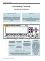
Input Signal Conditioning
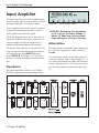
Input Amplifier
The input amplifiers are used for adapting the
widely varying signals in the ambient world to
the measuring logic of the timer/counter.
These amplifiers have many controls, and it is
essential to understand how these controls
work together and affect the signal.
The block diagram below shows the order in
which the different controls are connected. It
is not a complete technical diagram but intended to help understanding the controls.
The menus from which you can adjust the settings for the two main measurement channels
are reached by pressing INPUT A respectively INPUT B. See Figure 3-2. The active
choices are shown in boldface on the bottom
line.
Impedance
The input impedance can be set to 1 MW or
50 W by toggling the corresponding softkey.
Fig. 3-2
CAUTION: Switching the impedance
to 50 W when the input voltage is
above 12 VRMS may cause permanent damage to the input circuitry.
Attenuation
The input signal's amplitude can be attenuated
by 1 or 10 by toggling the softkey marked
1x/10x.
Use attenuation whenever the input signal exceeds the dynamic input voltage range ±5 V or
else when attenuation can reduce the influence
of noise and interference. See the section dealing with these matters at the end of this chapter.
A
B
Fig. 3-1
Block diagram of the signal conditioning.
3-2 Input Amplifier
Input settings menu.
Input Signal Conditioning
NOTE: For explanation of the hysteresis band,
see page 4-3.
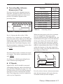
Coupling
Switch between AC coupling and DC coupling by toggling the softkey AC/DC.
DC Coupling
5V
AC Coupling
0V
Fig. 3-5
Fig. 3-3
AC coupling a symmetrical signal.
No triggering due to AC coupling
of signal with low duty cycle.
Filter
Use the AC coupling feature to eliminate unwanted DC signal components. Always use
AC coupling when the AC signal is superimposed on a DC voltage that is higher than the
trigger level setting range. However, we recommend AC coupling in many other measurement situations as well.
When you measure symmetrical signals, such
as sine and square/triangle waves, AC coupling filters out all DC components. This
means that a 0 V trigger level is always centered around the middle of the signal where
triggering is most stable.
If you cannot obtain a stable reading, the signal-to-noise ratio (often designated S/N or
SNR) might be too low, probably less than 6
to 10 dB. Then you should use a filter. Certain
conditions call for special solutions like
highpass, bandpass or notch filters, but usually the unwanted noise signals have higher
frequency than the signal you are interested
in. In that case you can utilize the built-in
lowpass filters. There are both analog and digital filters, and they can also work together.
Fig. 3-6
Fig. 3-4
Missing trigger events due to AC
coupling of signal with varying
duty cycle.
Signals with changing duty cycle or with a
very low or high duty cycle do require DC
coupling. Fig. 3-4shows how pulses can be
missed, while Fig. 3-5shows that triggering
does not occur at all because the signal amplitude and the hysteresis band are not centered.
The menu choices after selecting
FILTER.
n Analog Lowpass Filter
The counter has analog LP filters of RC type,
one in each of the channels A and B, with a
cutoff frequency of approximately 100 kHz,
and a signal rejection of 20 dB at 1 MHz.
Accurate frequency measurements of noisy
LF signals (up to 200 kHz) can be made when
the noise components have significantly
Input Amplifier 3-3
Input Signal Conditioning
higher frequencies than the fundamental signal.
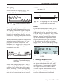
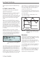
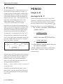
n Digital Lowpass Filter
The digital LP filter utilizes the Hold-Off
function described below.
With trigger Hold-Off it is possible to insert a
deadtime in the input trigger circuit. This
means that the input of the counter ignores all
hysteresis band crossings by the input signal
during a preset time after the first trigger
event.
When you set the Hold-Off time to approx.
75% of the cycle time of the signal, erroneous
triggering is inhibited around the point where
the input signal returns through the hysteresis
band. When the signal reaches the trigger
point of the next cycle, the set Hold-Off time
has elapsed and a new and correct trigger will
be initiated.
Instead of letting you calculate a suitable
Hold-Off time, the counter will do the job for
you by converting the filter cutoff frequency
you enter via the value input menu below to
an equivalent Hold-Off time.
Fig. 3-7
Value input menu for setting the
cutoff frequency of the digital filter.
You should be aware of a few limitations to be
able to use the digital filter feature effectively
and unambiguously. First you must have a
rough idea of the frequency to be measured. A
cutoff frequency that is too low might give a
perfectly stable reading that is too low. In such
a case, triggering occurs only on every 2nd,
3-4 Input Amplifier
3rd or 4th cycle. A cutoff frequency that is too
high (>2 times the input frequency) also leads
to a stable reading. Here one noise pulse is
counted for each half-cycle.
Use an oscilloscope for verification if you are
in doubt about the frequency and waveform of
your input signal..
The cutoff frequency setting range is very
wide: 1 Hz - 50 MHz
Hold-off time
Correct
measurement
Fig. 3-8
Digital LP filter operates in the
measuring logic, not in the input
amplifier.
Man/Auto
Toggle between manual and automatic triggering with this softkey. When Auto is active the
counter automatically measures the
peak-to-peak levels of the input signal and
sets the trigger level to 50% of that value. The
attenuation is also set automatically.
At rise/fall time measurements the trigger levels are automatically set to 10% and 90% of
the peak values.
When Manual is active the trigger level is set
in the value input menu designated Trig. See
below. The current value can be read on the
display before entering the menu.
Input Signal Conditioning
n Speed
The Auto-function measures amplitude and
calculates trigger level rapidly, but if you aim
at higher measurement speed without having
to sacrifice the benefits of automatic triggering, then use the Auto Trig Low Freq function to set the lower frequency limit for voltage measurement.
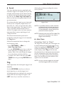
deleting the position preceding the current
cursor position.
Fig. 3-9
If you know that the signal you are interested
in always has a frequency higher than a certain value flow , then you can enter this value
from a value input menu. The range for flow is
1 Hz to 100 kHz, and the default value is
100 Hz. The higher value, the faster measurement speed due to more rapid trigger level
voltage detection.
Even faster measurement speed can be
reached by setting the trigger levels manually.
See Trig below.
Follow the instructions here to change the
low-frequency limit:
– Press SETTINGS ® Misc ®
Auto Trig Low Freq.
– Use the UP/DOWN arrow keys or the numeric input keys to change the low frequency limit to be used during the trigger
level calculation, (default 100 Hz).
– Confirm your choice and leave the SETTINGS menu by pressing EXIT/OK three
times.
Trig
Value input menu for setting the
trigger level.
NOTE: It is probably easier to make small adjustments around a fixed value by using the arrow keys for incrementation
or decrementation. Keep the keys depressed for faster response
NOTE: Switching over from AUTO to MAN Trigger Level is automatic if you enter a
trigger level manually.
n Auto Once
Converting “Auto” to “Fixed”
The trigger levels used by the auto trigger can
be frozen and turned into fixed trigger levels
simply by toggling the MAN/AUTO key. The
current calculated trigger level that is visible
on the display under Trig will be the new
fixed manual level. Subsequent measurements
will be considerably faster since the signal
levels are no longer monitored by the instrument. You should not use this method if the
signal levels are unstable.
NOTE: You can use auto trigger on one input
and fixed trigger levels on the other.
Value input menu for entering the trigger level
manually.
Use the UP/DOWN arrow keys or the numeric input keys to set the trigger level.
A blinking underscore indicates the cursor position where the next digit will appear. The
LEFT arrow key is used for correction, i.e.
Input Amplifier 3-5
Input Signal Conditioning
How to Reduce or
Ignore Noise and
Interference
Sensitive counter input circuits are of course
also sensitive to noise. By matching the signal
amplitude to the counter’s input sensitivity,
you reduce the risk of erroneous counts from
noise and interference. These could otherwise
ruin a measurement.
To ensure reliable measuring results, the counter has the following functions to reduce or
eliminate the effect of noise:
– 10x input attenuator
– Continuously variable trigger level
– Continuously variable hysteresis for some
functions
– Analog low-pass noise suppression filter
– Digital low-pass filter (Trigger Hold-Off)
To make reliable measurements possible on
very noisy signals, you may use several of the
above features simultaneously.
Optimizing the input amplitude and the trigger
level, using the attenuator and the trigger control, is independent of input frequency and
useful over the entire frequency range. LP filters, on the other hand, function selectively
over a limited frequency range.
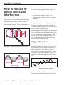
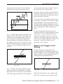
Trigger Hysteresis
Fig. 3-10
Narrow hysteresis gives erroneous triggering on noisy signals.
Fig. 3-11
Wide trigger hysteresis gives
correct triggering.
The signal needs to cross the 20 mV input
hysteresis band before triggering occurs. This
hysteresis prevents the input from self-oscillating and reduces its sensitivity to noise.
Other names for trigger hysteresis are “trigger
sensitivity” and “noise immunity”. They explain the various characteristics of the hysteresis.
Fig. 3-12
Erroneous counts when noise
passes hysteresis window.
Fig. 3-10 and Fig. 3-12 show how spurious
signals can cause the input signal to cross the
3-6 How to Reduce or Ignore Noise and Interference
Input Signal Conditioning
trigger or hysteresis window more than once
per input cycle and give erroneous counts.
do not attenuate the signal too much, and set
the sensitivity of the counter high.
In practice however, trigger errors caused by
erroneous counts (Fig. 3-10 and Fig. 3-12) are
much more important and require just the opposite measures to be taken.
To avoid erroneous counting caused by spurious signals, you need to avoid excessive input
signal amplitudes. This is particularly valid
when measuring on high impedance circuitry
and when using 1MW input impedance. Under
these conditions, the cables easily pick up
noise.
Fig. 3-13
Trigger uncertainty due to noise.
Fig. 3-13 shows that less noise still affects the
trigger point by advancing or delaying it, but
it does not cause erroneous counts. This trigger uncertainty is of particular importance
when measuring low frequency signals, since
the signal slew rate (in V/s) is low for LF signals. To reduce the trigger uncertainty, it is desirable to cross the hysteresis band as fast as
possible.
External attenuation and the internal 10x
attenuator reduce the signal amplitude, including the noise, while the internal sensitivity
control in the counter reduces the counter’s
sensitivity, including sensitivity to noise. Reduce excessive signal amplitudes with the 10x
attenuator, or with an external coaxial
attenuator, or a 10:1 probe.
How to use Trigger Level
Setting
For most frequency measurements, the
optimal triggering is obtained by positioning
the mean trigger level at mid amplitude, using
either a narrow or a wide hysteresis band, depending on the signal characteristics.
Fig. 3-14
Low amplitude delays the trigger point
Fig. 3-14 shows that a high amplitude signal
passes the hysteresis faster than a low amplitude signal. For low frequency measurements
where the trigger uncertainty is of importance,
Fig. 3-15
Timing error due to slew rate.
When measuring LF sine wave signals with
little noise, you may want to measure with a
How to Reduce or Ignore Noise and Interference 3-7
Input Signal Conditioning
tem makes many measurements per
second. Here you can increase the
measuring rate by switching off this
probing if the signal amplitude is constant. One single command and the
AUTO trigger function determines the
trigger level once and enters it as a
fixed trigger level.
high sensitivity (narrow hysteresis band) to reduce the trigger uncertainty. Triggering at or
close to the middle of the signal leads to the
smallest trigger (timing) error since the signal
slope is steepest at the sine wave center, see
Fig. 3-15.
When you have to avoid erroneous counts due
to noisy signals, see Fig. 3-12, expanding the
hysteresis window gives the best result if you
still center the window around the middle of
the input signal. The input signal excursions
beyond the hysteresis band should be equally
large.
n Auto Trigger
For normal frequency measurements, i.e.
without arming, the Auto Trigger function
changes to Auto (Wide) Hysteresis, thus widening the hysteresis window to lie between
70 % and. 30 % of the peak-to-peak amplitude. This is done with a successive approximation method, by which the signal’s MIN.
and MAX. levels are identified, i.e., the levels
where triggering just stops. After this
MIN./MAX. probing, the counter sets the trigger levels to the calculated values. The default
relative trigger levels are indicated by 70 %
on Input A and 30 % on Input B. These values
can be manually adjusted between 50 % and
100 % on Input A and between 0 % and 50 %
on Input B. The signal, however, is only applied to one channel.
Before each frequency measurement the counter repeats this signal probing to identify new
MIN/MAX values. A prerequisite to enable
AUTO triggering is therefore that the input
signal is repetitive, i.e., ³100 Hz (default).
Another condition is that the signal amplitude
does not change significantly after the measurement has started.
NOTE: AUTO trigger limits the maximum measuring rate when an automatic test sys-
n Manual Trigger
Switching to Man Trig also means Narrow
Hysteresis at the last Auto Level. Pressing
AUTOSET once starts a single automatic
trigger level calculation (Auto Once). This calculated value, 50 % of the peak-to-peak amplitude, will be the new fixed trigger level,
from which you can make manual adjustments
if need be.
n Harmonic Distortion
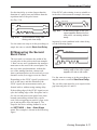
As rule of thumb, stable readings are free
from noise or interference.
However, stable readings are not necessarily
correct; harmonic distortion can cause erroneous yet stable readings.
Sine wave signals with much harmonic distortion, see Fig. 3-17, can be measured correctly
by shifting the trigger point to a suitable level
or by using continuously variable sensitivity,
see Fig. 3-16. You can also use Trigger
Hold-Off, in case the measurement result is
not in line with your expectations.
GOOD
BAD
Fig. 3-16
Variable sensitivity.
Fig. 3-17
Harmonic distortion.
3-8 How to Reduce or Ignore Noise and Interference
Chapter 4
Measuring Functions
Measuring Functions
Introduction to This Chapter
This chapter describes the different measuring
functions of the counter. They have been
grouped as follows:
Frequency measurements
– Frequency
– Period
– Ratio
– Burst frequency and PRF.
– FM
– AM
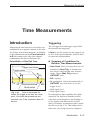
Time measurements
– Time interval.
– Pulse width.
– Duty factor.
– Rise/Fall time.
Phase measurements
Voltage measurements
– VMAX, VMIN.
– VPP.
4-2 Selecting Function
Selecting Function
See also the front panel layout on page 2-3 to
find the keys mentioned in this section together with short descriptions.
Press MEAS FUNC to open the main menu
for selecting measuring function. The two basic methods to select a specific function and
its subsequent parameters are described on
page 2-6.
Measuring Functions
Frequency Measurements
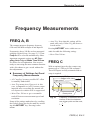
FREQ A, B
The counter measures frequency between
0 Hz and 300 MHz on Input A and Input B.
Frequencies above 100 Hz are best measured
using the Default Setup. See page 2-13. Then
Freq A will be selected automatically. Other
important automatic settings are AC Coupling, Auto Trig and Meas Time 200 ms.
See below for an explanation. You are now
ready to start using the most common function
with a fair chance to get a result without further adjustments.
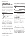
n Summary of Settings for Good
Frequency Measurements
– AC Coupling, because possible DC offset
is normally undesirable.
– Auto Trig. Note that this setting will be
made once only if Man Trig has been selected earlier.
Pressing AUTOSET twice within two seconds also adds the following setting:
– Meas Time 200 ms.
FREQ C
With an optional prescaler the counter can
measure up to 3 GHz or 8 GHz on Input C.
These RF inputs are fully automatic and no
setup is required.
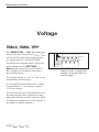
H y s te r e s is b a n d ( S E N S )
T r ig g e r le v e l o ffs e t
T r ig g e r p o in ts
– Auto Trig means Auto Hysteresis in this
case, (comparable to AGC) because superimposed noise exceeding the normal narrow hysteresis window will be suppressed.
0 V
R e s e t p o in ts
– Meas Time 200 ms to get a reasonable
tradeoff between measurement speed and
resolution.
Some of the settings made above by recalling
the Default Setup can also be made by activating the AUTOSET key. Pressing it once
means:
J
Fig. 4-1
Frequency is measured as the
inverse of the time between
one trigger point and the next;
1
f =
t
FREQ A, B 4-3
Measuring Functions
RATIO A/B, B/A,
C/A, C/B
cycles will be 3 x prescaling factor. The
3 GHz option, for example, has a prescaling
factor of 16 and requires at least 48 cycles in
each burst.
To find the ratio between two input frequencies, the counter counts the cycles on two
channels simultaneously and divides the result
on the primary channel by the result on the
secondary channel.
The minimum burst duration is 40 ns below
and 80 ns above 160 MHz.
Ratio can be measured between Input A and
Input B, where either channnel can be the primary or the secondary channel. Ratio can also
be measured between Input C and Input A or
between Input C and Input B. Here Input C is
the primary channel.
Note that the resolution calculations are very different as compared to frequency measurements. See page 8-10 for details.
+
BURST A, B, C
A burst signal as in Fig. 4-2 has a carrier wave
(CW) frequency and a modulation frequency,
also called the pulse repetition frequency
(PRF), that switches the CW signal on and off.
Both the CW frequency, the PRF, and the
number of cycles in a burst are measured
without external arming signals and with or
without selectable start arming delay. See
Chapter 5 “Measurement Control” for a fundamental discussion of arming and arming delay.
The general frequency limitations for the respective measuring channel also apply to burst
measurements. The minimum number of cycles in a burst on Input A or Input B is 3 below 160 MHz and 6 between 160 MHz and
300 MHz. Burst measurements on Input C involve prescaling, so the minimum number of
4-4 RATIO A/B, B/A, C/A, C/B
Triggering
Bursts with a PRF above 50 Hz can be measured with auto triggering on.
The out-of-sync error described under heading
“Possible errors” on page 4-6may occur more
frequently when using Auto Trigger.
When PRF is below 50 Hz and when the gap
between the bursts is very small, use manual
triggering.
Always try using AUTOSET first. Then the
Auto Trigger and the Auto Sync functions in
combination will give satisfactory results
without further tweaking in most cases. Sometimes switching from AUTO to MANual triggering in the INPUT A/B menus is enough to
get stable readings. The continually calculated
trigger levels will then be fixed.
Input C has always automatic triggering and
AUTOSET only affects the burst synchronization.
C W
B u rs t
S ig n a l
P R F
Fig. 4-2
Burst signal.
Measuring Functions
Burst Measurements using
Manual Presetting
n Selecting Measurement Time
You can measure the frequency on Input A
and Input B to 300 MHz and on Input C with
limited specifications to the upper frequency
limit of the prescaler with the internally synchronized BURST function as follows:
– Select Freq Burst under the Freq menu
– Select A, B, or C as measurement input.
– Press SETTINGS and Burst. Select a
Meas Time that is shorter than the burst
duration minus two CW cycles.
If you do not know the approximate burst parameters of your signal, always start with a
short measurement time and increase it gradually until the readout gets unstable.
– Press Sync Delay and enter a value longer than the burst duration and shorter
than the inverse of the PRF. See Fig. 4-3.
B u rs t
S ig n a l
Fig. 4-3
S y n c . d e la y
Set the sync delay so that it expires in the gap between the
bursts.
Fig. 4-4
Three time values must be set to
measure the correct part of a
burst
The measurement time must be shorter than
the duration of the burst. If the measurement
continues during part of the burst gap, no matter how small a period of time, then the measurement is ruined. Choosing a measurement
time that is too short is better since it only reduces the resolution. Making burst frequency
measurements on short bursts means using
short measurement times, giving a poorer resolution than normally achieved with the counter.
n How Does the Sync Delay
Work?
– Press Start Delay and enter a value longer than the transient part of the burst
pulse.
– Select Frequency Limit (160/300 MHz)
if Input A or Input B is to be used. Use
the low limit if possible to minimize the
number of cycles necessary to make a
measurement.
The sync delay works as an internal start arming delay: it prevents the start of a new measurement until the set sync delay has expired.
See Fig. 4-5.
After the set measurement time has started,
the counter synchronizes the start of the measurement with the second trigger event in the
burst. This means that the measurement does
– Press EXIT/OK to measure.
All relevant burst parameters can be read on
the display simultaneously.
BURST A, B, C 4-5
Measuring Functions
not start erroneously during the Burst Off duration or inside the burst.
M e a s u re
S y n c - d e la y
G a te T im e
Fig. 4-5
Frequency
Modulated Signals
A frequency modulated signal is a carrier
wave signal (CW frequency = f0) that changes
in frequency to values higher and lower than
the frequency f0. It is the modulation signal
that changes the frequency of the carrier
wave.
The counter can measure:
Measuring the frequency of the
carrier wave signal in a burst.
f0 = Carrier frequency.
fmax = Maximum frequency.
n Possible Errors
Before the measurement has been synchronized with the burst signal, the first measurement(s) could start accidentally during the
presence of a burst. If this would happen and
if the remaining burst duration is shorter than
the set measurement time, the readout of the
first measurement will be wrong. However,
after this first measurement, a properly set
start-arming sync delay time will synchronize
the next measurements.
In manually operated applications, this is not a
problem. In automated test systems where the
result of a single measurement sample must be
reliable, at least two measurements must be
made, the first to synchronize the measurement and the second from which the measurement result can be read out.
fmin = Minimum frequency.
Df = Frequency swing = fmax – f0.
Carrier Wave Frequency f0
To determine the carrier wave frequency, measure fmean which is a close approximation of
f0.
Press STAT/PLOT to get an overview of all
the statistical parameters.
Select the measurement time so that the counter measures an integral number of modulation
periods. This way the positive frequency deviations will compensate the negative deviations
during the measurement.
Example: If the modulation frequency is
50 Hz, the measurement time 200 ms will
make the counter measure 10 complete modulation cycles.
If the modulation is non-continuous, like a
voice signal, it is not possible to fully compensate positive deviations with negative
deviations. Here, part of a modulation swing
4-6 Frequency Modulated Signals
Measuring Functions
may remain uncompensated for, and lead to a
measuring result that is too high or too low.
W o r s t C a s e M e a s u r in g T im e
D u r a tio n , w h e r e
fm
a x
D fm
a x
f0
fm
Fig. 4-6
e a n
= f0
{
M o d u la tio n s ig n a l
f m o d u la tio n
fm
in
Frequency modulation
In the worst case, exactly half a modulation
cycle would be uncompensated for, giving a
maximum uncertainty of:
f0 - fmean = ±
tmeasuring
Dfmax
´ fmod ulation ´ p
For very accurate measurements of the carrier
wave frequency f0, measure on the
unmodulated signal if it is accessible.
n Modulation Frequencies
above 1 kHz
– Turn off SINGLE.
– Set a long measurement time that is an
even multiple of the inverse of the modulation frequency.
You will obtain a good approximation when
you select a long measurement time, for instance 10 s, and when the modulation frequency is high, above 1000 Hz.
n Low Modulation Frequencies
Press SETTINGS ® STAT and make the
No. of samples parameter as large as possible considering the maximum allowed measurement time. Press STAT/PLOT and let the
counter calculate the mean value of the samples.
You will usually get good results with 0.1 s
measurement time per sample and more than
30 samples (n ³ 30). You can try out the optimal combination of sample size and measurement time for specific cases. It depends on the
actual f0 and Dfmax.
Here the sampling frequency of the measurement (1/measurement time) is asynchronous
with the modulation frequency. This leads to
individual measurement results which are randomly higher and lower than f0. The statistically averaged value of the frequency fmean
approaches f0 when the number of averaged
samples is sufficiently large.
When the counter measures instantaneous frequency values (when you select a very short
measurement time), the RMS measurement
uncertainty of the measured value of f0 is:
f0 - fmean = ±
1
´ D fmax
2n
where n is the number of averaged samples of
f.
fmax
– Press SETTINGS ® STAT and set No.of
samples to 1000 or more.
– Press Meas Time and select a low value.
– Press STAT/PLOT and watch fmax.
fmin
– Press SETTINGS ® STAT and set No.of
samples to 1000 or more.
– Press Meas Time and select a low value.
– Press STAT/PLOT and watch fmin.
Frequency Modulated Signals 4-7
Measuring Functions
Dfp-p
– Press SETTINGS ® STAT and set No.of
samples to 1000 or more.
– Press Meas Time and select a low value.
Press STAT/PLOT and watch Dfp-p.
Df p - p = fmax - fmin = 2 ´ Df .
Errors in fmax, fmin, and Dfp-p
are much like the burst measurements described earlier in this manual.
Carrier Wave Frequency
The carrier wave (CW) is only continuously
present in a narrow amplitude band in the
middle of the signal if the modulation depth is
high. If the sensitivity of the counter is too
low, cycles will be lost, and the measurement
ruined.
A measurement time corresponding to 110cycle, or 36° of the modulation signal, leads to
an error of approx 1.5%.
Select the measurement time:
tmeasure £
1
10 ´ fmodulation
f
< 0 .0 0 7 B
M o d u la tio n
s ig n a l
Fig. 4-8
B
A /1 0
Effects of different sensitivity
when measuring the CW Frequency of an AM signal.
t
To measure the CW frequency:
A
Fig. 4-7
Error when determining fmax
– Enter the INPUT A menu.
– Select a measurement time that gives you
the resolution you want.
To be confident that the captured maximal frequency really is fmax, you must select a sufficiently large number of samples, for instance
n ³ 1000.
– Turn on Manual trigger.
– Press Trig level and enter 0 V trigger
level (press the numeric key 0 and
EXIT/OK).
– Select AC coupling.
– Select 1x attenuation to get a narrow hys-
AM Signals
The counter can usually measure both the carrier wave frequency and modulation frequency of AM signals. These measurements
4-8 AM Signals
teresis band.
– If the counter triggers on noise, widen the
hysteresis band with the ‘variable hysteresis’ function, i.e. enter a trigger level
>0 V but <VP-Pmin. See Fig. 4-8.
Measuring Functions
Modulating Frequency
The easiest way to measure the modulating
frequency is after demodulation, for instance
by means of a so-called RF-detector probe
(also known as a demodulator probe, e.g.
Pomona type 5815) used with AC-coupling of
the input channel. If no suitable demodulator
is available, use the Freq Burst function to
measure the modulation frequency in the same
way as when measuring Burst PRF.
S y n c . d e la y
M e a s u r e d c y c le s
Fig. 4-9
Measuring the modulating frequency.
Theory of
Measurement
Reciprocal Counting
Simple frequency counters count the number
of input cycles during a preset gate time, for
instance one second. This leads to a ± 1 input
cycle count error that, at least for low-frequency measurements, is a major contribution
to uncertainty.
However, the counters described here use a
high-resolution, reciprocal counting technique, synchronizing the measurement start
with the input signal. In this way an exact
number of integral input cycles will be
counted, thereby omitting the ± 1 input cycle
error.
S e t M e a s u r in g T im e
– Press MEAS FUNC and select
t1
Freq Burst A.
t2
– Press SETTINGS ® Burst ® Meas
Time and enter a measurement time that
is approximately 25 % of the modulating
period.
– Press Sync Delay and enter a value that
is approximately 75 % of the modulating
period. See Fig. 4-3.
– Press INPUT A and turn on Manual trigger.
– Press Trig and enter a trigger level that
makes the counter trigger according to
Fig. 4-9.
Even though the main frequency reading may
now be unstable, the PRF value on the display
will represent the modulating frequency.
A c tu a l G a te
T im e
Fig. 4-10
tg
Synchronization of a measurement.
After the start of the set measurement time,
the counter synchronizes the beginning of the
actual gate time with the first trigger event (t1)
of the input signal. See also Fig. 4-10.
In the same way, the counter synchronizes the
stop of the actual gate time with the input signal, after the set measurement time has
elapsed. The multi-register counting technique
allows you to simultaneously measure the ac-
Theory of Measurement 4-9
Measuring Functions
tual gate time (tg) and the number of cycles
(n) that occurred during this gate time.
When no triggering has occurred during the
time-out, the counter will show NO SIGNAL.
Thereafter, the counter calculates the frequency according to Mr. Hertz’s definition:
Measuring Speed
f =
n
tg
The '90' measures the gate time, tg, with a resolution of 100 ps, independent of the measured frequency. Consequently the use of
prescalers does not influence the quantization
error. Therefore, the relative quantization error
is: 100 ps/tg.
For a 1-second measurement time, this value
is:
100 ps
= 100 ´ 10-12 = 1 ´ 10-10
1s
Except for very low frequencies, tg and the set
measurement time are nearly identical.
Sample-Hold
If the input signal disappears during the measurement, the counter will behave like a voltmeter with a sample-and-hold feature and will
freeze the result of the previous measurement.
Time-Out
Mainly for GPIB use, you can manually select
a fixed time-out in the menu reached by pressing SETTINGS ® Misc ® Timeout. The
range of the fixed timeout is 10 ms to 1000 s,
and the default setting is Off.
Select a time that is longer than the cycle time
of the lowest frequency you are going to measure; multiply the time by the prescaling factor of the input channel and enter that time as
time-out.
4-10 Theory of Measurement
The set measurement time determines the
measuring speed for those functions that utilize averaging – Frequency and Period
Avg. For continuous signals,
1
readings/s
Speed »
tg + 0.2
when Auto trigger is on and can be increased
to:
1
readings/s
Speed »
tg + 0.001
when Manual trigger is on, or via GPIB:
1
readings/s
Speed »
tg + 0.00012
n Average and Single Cycle
Measurements
To reduce the actual gate time or measuring
aperture, the counters have very short measurement times and a mode called Single for
period measurements. The latter means that
the counter measures during only one cycle of
the input signal. In applications where the
counter uses an input channel with a prescaler,
the Single measurement will last as many cycles as the division factor. If you want to measure with a very short aperture, use an input
with a low division factor.
Averaging is the normal mode for frequency
and period measurements when you want to
reach maximum resolution. There is always a
tradeoff between time and precision, however,
so decide how many digits you need and use
as short a measurement time as possible to arrive at your objective.
Measuring Functions
n Prescaling May Influence
Function
Prescaling
Factor
FREQ A/B (300 MHz)
2
Measurement Time
Prescalers do affect the minimum measurement time, inasmuch as short bursts have to
contain a minimum number of carrier wave
periods. This number depends on the
prescaling factor.
f
In p u t
s ig n a l
A fte r
p r e s c a le r
f/1 6
1 6 p e r io d s
Fig. 4-11
BURST A/B (<160 MHz)
1
BURST A/B (>160 MHz
2
PERIOD A/B AVG (300 MHz)
2
PERIOD A/B SGL (300 MHz)
1
FREQ C (3 GHz)
16
FREQ C (8 GHz)
256
All other functions
1
Table 4-1
Prescaling factors.
Divide-by-16 Prescaler
Fig. 4-11 shows the effect of the 3 GHz
prescaler. For 16 input cycles, the prescaler
gives one square wave output cycle. When the
counter uses a prescaler, it counts the number
of prescaled output cycles, here f/16. The display shows the correct input frequency since
the microcomputer compensates for the effect
of the division factor d as follows:
n´d
f =
tg
Prescalers do not reduce resolution in reciprocal counters. The relative quantization error is
100 ps
still:
tg
See Table 4-1 to find the prescaling factors
used in different operating modes.
When measuring pulses with a low repetition
rate, for example a 0.1 Hz pulse with a
non-prescaled function like PERIOD SGL, the
measurement will require at least the duration
of one cycle, that is 10 seconds, and at worst
nearly 20 seconds. The worst case is when a
trigger event took place just before the beginning of a measurement time (Fig. 4-12). Measuring the frequency of the same signal will
take twice as long, since this function involves
prescaling by a factor two.
P o s s ib le tr ig g e r e v e n ts
S e t m e a s u r in g
tim e
n LF Signals
Signals below 100 Hz should be measured
with manual triggering, unless the default setting (100 Hz) is changed. See page 2-11. The
low limit can be set to 1 Hz, but the measurement process will be slowed down considerably if auto triggering is used in conjunction
with very low frequencies.
G a te tim e
T im e fo r o n e m e a s u r e m e n t
Fig. 4-12
Measurement Time
Even if you have chosen a short measurement
time, this measurement will require between
20 and 40 seconds (for this example).
Theory of Measurement 4-11
Measuring Functions
n RF Signals
As mentioned before, a prescaler in the C-input divides the input frequency before it is
counted by the normal digital counting logic.
The division factor is called prescaler factor
and can have different values depending on
the prescaler type. The 3 GHz prescaler is designed for a prescaling factor of 16. This
means that an input C frequency of, e.g.,
1.024 GHz is transformed to 64 MHz.
Prescalers are designed for optimum performance when measuring stable continuous RF.
Most prescalers are inherently unstable and
would self-oscillate without an input signal.
To prevent a prescaler from oscillating, a
“go-detector” is incorporated. See Fig. 4-13.
The go-detector continuously measures the
level of the input signal and simply blocks the
prescaler output when no signal, or a signal
that is too weak, is present.
+ N
&
T o c o u n tin g
lo g ic
G o -d e te c to r
Fig. 4-13
Go-detector in the prescaler
The presence of a burst signal to be measured
makes certain demands upon the signal itself.
Regardless of the basic counter’s ability to
measure during very short measurement
times, the burst duration must meet the following minimum conditions:
Burstmin > ( presc. factor) ´ (inp. cycle time) ´ 3
or at least 80 ns
Normally the real minimum limit is set by
other factors, like the speed of the GO-detector. This speed depends on the specific input
option used.
4-12 PERIOD
PERIOD
Single A, B
Average A, B, C
From a measuring point of view, the period
function is identical to the frequency function.
This is because the period of a cyclic signal
has the reciprocal value of the frequency ( 1 f ).
In practice there are two minor differences.
1. The counter calculates FREQUENCY
(always AVG) as:
f =
number of cycles
actual gate time
while it calculates PERIOD AVG as:
p=
actual gate time
number of cycles
2. In the PERIOD SINGLE mode, the counter uses no prescaler.
All other functions and features as described
earlier under “Frequency” apply to Period
measurements.
Measuring Functions
Time Measurements
Introduction
Measuring the time between a start and a stop
condition on two separate channels is the basis
for all time interval measurements. In addition
to the fundamental function Time Interval A
to B, the counters also offer other channel
combinations and derived functions like
Pulse Width and Rise/Fall Time.
H y s te r e s is b a n d ( S E N S )
T r ig g e r le v e l o ffs e t
T r ig g e r p o in ts
J
Triggering
The set trigger level and trigger slope define
the start and stop triggering.
If Auto is on, the counter sets the trigger level
to 50% of the signal amplitude, which is ideal
for most time measurements.
n Summary of Conditions for
Reliable Time Measurements:
– Auto Once, that is freezing the levels determined by Auto Trig, is normally the
best choice when making time measurements. Choose Man Trig and press
AUTOSET once.
– DC coupling.
– 1x Attenuation. Selected automatically if
0 V
R e s e t p o in ts
Fig. 4-14
Time is measured between the trigger point and the reset
point. Accurate measurements are
possible only if the hysteresis band is
narrow.
AUTOSET was used before to set the
trigger levels.
– High signal level.
– Steep signal edges.
Even though the input amplifiers have high
sensitivity, the hysteresis band has a finite
value that would introduce a small timing error for signals with different rise and fall
times, for instance asymmetrical pulse signals
like the one in Fig. 4-14. This timing error is
taken care of by using hysteresis compensa-
Introduction 4-13
Measuring Functions
tion that virtually moves the trigger points by
half the hysteresis band.
Rise and fall time can be measured on both input A and input B.
Time Interval
By convention, rise/fall time measurements
are made with the trigger levels set to 10 %
(start) and 90 % (stop) of the maximum pulse
amplitude, see Figure 4-15.
All time interval functions can be found under
the function menu Time.
The toggling SLOPE keys (marked with a
positive
or negative
edge symbol) under the menus INPUT A/B decide which edge
of the signal will start resp. stop the measurement.
The counter measures the time from when the
signal passes 10 % of its amplitude to when it
passes 90 % of its amplitude. The trigger levels are calculated and set automatically.
Auxiliary parameters shown simultaneously
are Slew Rate (V/s), Vmax and Vmin
1 0 0 %
T r ig g e r L e v e l B
Time Interval A to B
The counter measures the time between a start
condition on input A and a stop condition on
input B.
9 0 %
In p u t A / C o m m o n B
T r ig g e r L e v e l A
1 0 %
0 %
Time Interval B to A
The counter measures the time between a start
condition on input B and a stop condition on
input A.
Time Interval A to A, B to B
When the same (common) signal source supplies both start and stop trigger events, connect the signal to either input A or input B.
These functions can be used for measuring
rise and fall times between arbitrary trigger
levels.
Rise/Fall Time A/B
These functions can be found under the function menu Time.
4-14 Time Interval
Fig. 4-15
Trigger levels for rise/fall measurements.
For ECL circuits, the reference levels are
20 % (start) and 80 % (stop). In this case you
can use either of two methods:
1. Select the general Time Interval function described above and set the trigger levels manually after calculating them from the absolute peak values. Then you can benefit from
the auxiliary parameters Vmax and Vmin. For
measurements made on input A, use the following settings:
Rise Time:
Trig Level A = Vmin +0.2(Vmax - Vmin)
Trig Level B = Vmin +0.8(Vmax - Vmin)
Fall Time:
Trig Level A = Vmin +0.8(Vmax - Vmin)
Trig Level B = Vmin +0.2(Vmax - Vmin)
2. Select one of the dedicated Rise/Fall Time
functions, and exploit the possibility to man-
Measuring Functions
ually adjust the relative trigger levels (in %)
when Auto Trigger is active. Both input
channel menus are used for entering the levels, but only one channel is the active signal
input.
See the paragraph on Auto Trigger (page 4-16)
to find out how overshoot or ringing may affect your measurement.
Pulse Width A/B
The function menu designation is Pulse. Either input A or input B can be used for measuring, and both positive and negative pulse
width can be selected.
– Positive pulse width means the time between a rising edge and the next falling
edge.
– Negative pulse width means the time between a falling edge and the next rising
edge.
The selected trigger slope is the start trigger
slope. The counter automatically selects the
inverse polarity as stop slope.
Duty factor =
+
Pulse width
Period
The total measurement time will
be doubled compared to a single
measurement, because "Duty"
requires 2 measurement steps.
Measurement
Errors
Hysteresis
The trigger hysteresis, among other things,
causes measuring errors, see Figure 4-16. Actual triggering does not occur when the input
signal crosses the trigger level at 50 percent of
the amplitude, but when the input signal has
crossed the entire hysteresis band.
S ta rt
C h a n n e l A
T r ig g e r le v e l
S to p
C h a n n e l B
M e a s u r e d T im e In te r v a l
Duty Factor A/B
Fig. 4-16
The function menu designation is Duty. Either input A or input B can be used for measuring, and both positive and negative duty
factor can be selected. See the preceding paragraph for a definition of positive and negative
in this context.
Duty factor (or duty cycle) is the ratio between pulse width and period time. The counter determines this ratio by first making a
pulse width measurement, then a period measurement, and calculates the duty factor as:
Trigger hysteresis
The hysteresis band is about 20 mV with attenuation 1x, and 200 mV with attenuation
10x.
To keep this hysteresis trigger error low, the
attenuator setting should be 1x when possible.
Use the 10x position only when input signals
have excessively large amplitudes, or when
you need to set trigger levels higher than 5 V.
Pulse Width A/B 4-15
Measuring Functions
Overdrive and Pulse
Rounding
Additional timing errors may be caused by
triggering with insufficient overdrive, see Figure 4-17. When triggering occurs too close to
the maximum voltage of a pulse, two phenomena may influence your measurement uncertainty: overdrive and rounding.
Auto Trigger is a great help especially when
you measure on unknown signals. However,
overshoot and ringing may cause Auto to
choose slightly wrong MIN and MAX signal
levels. This does not affect measurements like
frequency, but transition time measurements
may be affected.
Therefore, when working with known signals
such as logic circuitry, set the trigger levels
manually.
T r ig g e r le v e l
A c tu a l tr ig g e r in g
C r o s s in g tr ig g e r le v e l
Fig. 4-17
Auto Trigger
Insufficient overdrive causes
Trigger Error.
Overdrive: When the input signal crosses
the hysteresis band with only a marginal overdrive, triggering may take
some 100 ps longer than usual. The
specified worst case 500 ps systematic trigger error includes this error, but
you can avoid it by having adequate
overdrive.
Rounding: Very fast pulses may suffer
from pulse rounding, overshoot, or
other aberrations. Pulse rounding can
cause significant trigger errors, particularly when measuring on fast circuitry.
4-16 Measurement Errors
Always use manual trigger levels if the signal
repetition rate drops below 100 Hz (default),
or below the low frequency limit set by entering a value between 1 Hz and 50 kHz in the
menu Auto Trig Low Freq. You can reach it
by pressing SETTINGS ® Misc.
Measuring Functions
Phase
What is Phase?
Phase is the time difference between two signals of the same frequency, expressed as an
angle.
A
B
A somewhat more elaborate method is used in
these counters. It allows the necessary measurements to be performed in one pass by using time-stamping. Two consecutive
time-stamps from trigger events on channel A
and two corresponding time-stamps from
channel B are enough to calculate the result,
including sign.
Resolution
Phase?
A
Fig. 4-18
Phase delay.
P e r io d ( T )
The traditional method to measure phase delay with a timer/counter is a two-step process
consisting of two consecutive measurements,
first a period measurement and immediately
after that a time interval measurement. The
phase delay is then mathematically calculated
as:
360° ´ (Time Interval A - B )
Period
or in other words:
Phase A - B = 360°´ Time Delay ´ FREQ
B
T im e d e la y ( D t)
Fig. 4-19
f = D t * 3 6 0
T
o
Traditional phase definition.
The frequency range for phase is up to
160 MHz and the resolution depends on the
frequency. For frequencies below 100 kHz the
resolution is 0.001° and for frequencies above
10 MHz it is 1°. It can be further improved by
averaging through the built-in statistics functions.
What is Phase? 4-17
Measuring Functions
Possible Errors
n Random Errors
Phase can be measured on input signal frequencies up to 160 MHz. However, at these
very high frequencies the phase resolution is
reduced to:
100 ps ´ 360o ´ FREQ
100 ps ´ FREQ ´ 360°
Inaccuracies
The trigger noise error consists of start and
stop trigger errors that should be added. For
sinusoidal input signals each error is:
The inaccuracy of Phase A-B measurements
depends on several external parameters:
– Input signal frequency
– Peak amplitude and slew rate for input signals A and B
– Input signal S/N-ratio
Some internal parameters are also important:
– Internal time delay between channel A and
B signal paths
– Variations in the hysteresis window between channel A and B
Let us look deeper into the restrictions and
possibilities of using phase measurements.
Inaccuracy: The measurement errors are of
two kinds:
– Random errors
– Systematic errors
The random errors consist of resolution
(quantization) and noise trigger error.
Systematic errors consist of “inter-channel delay difference” and “trigger level timing” errors. Systematic errors are constant for a given
set of input signals, and in general, you can
compensate for them in the controller
(GPIB-systems) or locally via the MATH/LIM
menu (manual operation) after making calibration measurements. See Methods of Compensation on page 4-20.
4-18 Possible Errors
The phase quantization error algorithm is:
For example, the quantization error for a
1 MHz input signal is thus:
100 ps ´ 1 ´ 106 ´ 360° » 0.04 °
360°
2 p ´ S N ratio
Let’s use the example above and add some
noise so that the S/N ratio will be 40 dB. This
corresponds to an amplitude ratio of 100 times
(and power ratio of 10000 times). Then the
trigger noise will contribute to the random error with:
360°
» 0.6°
2 p ´ 100
The sum of random errors should not be added
linearly, but in an “RMS way”, because of
their random nature. Let’s do so for our examples above.
Measuring Functions
Random error =
quant. err.2 + start trg. err.2 + stop trg. err.2
The total random errors are thus:
0.04 2 + 0.62 + 0.62 » 0.85° (single-shot)
What about random errors caused by internal
amplifier noise? Internal noise contribution is
normally negligible. The phase error caused
by noise on the signal, whether internal or external, is:
<0.5 ns ´360°´ FREQ
See the following table.
The “trigger level timing error” is depending
on two factors:
For an input signal of 250 mVrms and the typical internal noise figure of 250 mVrms gives us
a S/N-ratio of a minimum of 60 dB (1000
times). This gives us a worst case error of
0.06°. Increasing the input signal to 1.5 Vrms
decreases the error to 0.01°.
Another way to decrease random errors is to
use the statistics features of the instrument and
calculate the mean value from a number of
samples.
n Systematic Errors in Phase
Measurements
160 MHz
28.8°
100 MHz
18.0°
10 MHz
1.8°
1 MHz
0.18°
100 kHz
0.018°
Table 4-2
due to trigger level uncertainty.
The inter-channel propagation delay difference is typically 500 ps at identical trigger
conditions in both input channels. Therefore,
the corresponding Phase difference is:
Trigger level timing error
360°
2p ´ S N ratio
10 kHz
– Inter-channel propagation delay difference.
– Trigger level timing errors (start and stop),
and below
0.002°
Phase difference caused by
inter-channel propagation delay
difference
Systematic errors consist of 3 elements:
– The actual trigger point is not exactly
zero, due to trigger level DAC uncertainty
and comparator offset error.
– The two signals have different slew rates
at the zero-crossing.
Every counter has input hysteresis. This is
necessary to prevent noise to cause erroneous
input triggering. The width of the hysteresis
band determines the maximum sensitivity of
the counter. It is approximately 30 mV, so
when you set a trigger level of 0 V, the actual
trigger point would normally be +15 mV and
the recovery point –15 mV. This kind of timing error is cancelled out by using hysteresis
compensation.
Hysteresis compensation means that the microcomputer can offset the trigger level so that
actual triggering (after offset) equals the set
trigger level (before offset). This general hysteresis compensation is active in phase as well
as in time interval and rise/fall time measurements. There is a certain residual uncertainty
of a few mV and there is also a certain temperature drift of the trigger point.
The nominal trigger point is 0 V with an uncertainty of ± 10 mV.
Possible Errors 4-19
Measuring Functions
A sine wave expressed as
described below. The first one is very simple
but does not take the inter-channel propagation delay difference into account. The second
one includes all systematic errors, if it is carried out meticulously, but it is often not practicable.
10 mV
(s)
(VP ´ 2p ´ FREQ )
Common settings for the two inputs are:
DV
of
V (t ) = VP ´ sin (2pft ), has a slew rate
Dt
VP ´ 2pf close to the zero-crosssing. That gives
us the systematic time error when crossing
10 mV, instead of crossing 0 mV.
And the corresponding phase error in degrees
is:
10 mV ´ 360° ´ FREQ
VP ´ 2p ´ FREQ
Slope:
Coupling:
Impedance:
Trigger:
Trigger Level:
Filter:
Pos or Neg
AC
1 MW or 50 W depending
on source and frequency
Man
0V
Off
which can be reduced to:
Method 1:
0.6
(° )
VP
This error can occur on both inputs, so the
worst case systematic error is thus:
0.6
0.6
+
(° )
VP ( A ) VP ( B )
Vpeak
(A)
Vpeak
(B)
Worst case
systematic error
150 mV
150 mV
4°+ 4° = 8°
1.5 V
150 mV
0.4°+ 4° = 4.4°
1.5 V
1.5 V
0.4°+ 0.4°= 0.8°
Table 4-3
Systematic trigger level timing
error (examples).
n Methods of Compensation
The calculations above show the typical uncertainties in the constituents that make up the
total systematic error. For a given set of input
signals you can compensate for this error
more or less completely by making calibration
measurements. Depending on the acceptable
residual error, you can use one of the methods
4-20 Possible Errors
Connect the test signals to Input A and Input
B. Select the function Phase A rel A to find
the initial error. Use the MATH/LIM menu to
enter this value as the constant L in the formula K*X+L by pressing X0 and change sign.
Now the current measurement result (X0) will
be subtracted from the future phase measurements made by selecting Phase A rel B. A
considerable part of the systematic phase errors will thus be cancelled out. Note that this
calibration has to be repeated if the frequency
or the amplitude changes.
Method 2:
Connect one of the signals to be measured to
both Input A and Input B via a 50 W power
splitter or a BNC T-piece, depending on the
source impedance. Make sure the cable
lengths between power splitter / T-piece and
instrument inputs are equal. Select the function Phase A rel B and read the result. Enter
this value as a correction factor in the same
way as described above for Method 1.
In order to minimize the errors you should
also maintain the signal amplitudes at the in-
Measuring Functions
puts, so that the deviation between calibration
and measurement is kept as small as possible.
The same restrictions as for Method 1 regarding frequency and amplitude apply to this
method, i.e. you should recalibrate whenever
one of these signal parameters changes.
Residual Systematic Error:
By mathematically (on the bench or in the
controller) applying corrections according to
one of the methods mentioned above, the systematic error will be reduced, but not fully
eliminated. The residual time delay error will
most probably be negligible, but a trigger
level error will always remain to a certain extent, especially if the temperature conditions
are not constant.
Possible Errors 4-21
Measuring Functions
Voltage
VMAX, VMIN, VPP
Press MEAS FUNC ® Volt. The counter can
measure the input voltage levels VMAX , VMIN
and VPP on DC-input voltages and on repetitive signals between 1 Hz and 300 MHz.
The voltage capacity is –50 V to +50 V in two
automatically selected ranges.
For LF signals the measurement has “voltmeter performance”, i.e. an accuracy of about
1 % of the reading.
You can select any one of the parameters to be
the main parameter that is displayed in large
digits and with full resolution, while the others
are displayed simultaneously at the bottom of
the display in smaller characters.
4-22 VMAX, VMIN, VPP
0 V
5 :th
4 :th
3 :rd
2 :n d
1 :s t
The default low frequency limit is 20 Hz but
can be changed via the SETTINGS ®
Miscellaneous menu between 1 Hz and 50
kHz. A higher low-frequency limit means
faster measurements.
+ V p e a k
Fig. 4-20
The voltage is determined by
making a series of trigger level
settings and sensing when the
counter triggers.
Measuring Functions
VRMS
When the waveform (e.g. sinusoidal, triangular, square) of the input signal is known, its
crest factor, defined as the quotient(QCF) of
the peak (Vp) and RMS (Vrms) values, can be
used to set the constant K in the mathematical
function K*X+L. The display will then show
the actual Vrms value of the input signal, assuming that Vpp is the main parameter.
Vrms =
1
V pp
2QCF
EXAMPLE: A sine wave has a crest factor of
1.414 ( 2), so the constant in the formula above will be 0.354.
Press MATH/LIM and after that
Math®Math(Off)®K*X+L Press K=
and enter 0.354 via the NUMERIC
ENTRY keys. Check that the L constant is set to its default setting 0. Confirm your choices with the softkeys below the display. If the input is AC coupled and Vpp selected, the display will
now show the RMS value of any sine
wave input.
If the sine wave is superimposed on a DC
voltage, the RMS value is found as:
0.354*Vpp + VDC. If VDC is not known it can
be found as:
VDC =
VMAX - VMIN
2
To display the rms value of a sine wave superimposed on a DC voltage, follow the example
above, but set L = VDC.
VRMS 4-23
Measuring Functions
This page is intentionally left blank.
4-24 VRMS
Chapter 5
Measurement Control
Measurement Control
About This Chapter
This chapter explains how you can control the
start and stop of measurements and what you
can obtain by doing so. The chapter starts by
explaining the keys and the functions behind
them, then gives some theory, and ends with
actual measurement examples.
Measurement Time
shows the results from a single input cycle.
The exceptions are Frequency and Period
Average.
Single or Average is not relevant for Vmax,
Vmin or Vpp measurements.
Hold/Run & Restart
Pressing HOLD completes the current measurement and freezes the result on the display.
This parameter is only applicable to the functions Frequency and Period Average. Increasing the measurement time gives more
digits, i.e. higher resolution, but fewer measurements per second. The default value is
200 ms but can be changed via SETTINGS
® Meas Time between 20 ns and 1000 s.
Pressing RESTART initiates a new measurement.
The default value gives 11 digits on the display and 4 to 5 measurements each second.
Varying the measurement time is a hardwarebased averaging method in contrast to the
software-based mean value function that can
be found in the STAT/PLOT menu.
Pressing RESTART starts a new measurement
from sample 1, and the measurement will stop
when the preset number of samples has been
taken.
The measurement time changes in 1/2/5 steps
if you use the arrow keys for stepping. By using the numeric entry keys you can set any
value within the specified range with a resolution of 20 ns.
To quickly select the lowest measurement time, enter 0. The
counter will select 20 ns automatically.
Arming gives you the opportunity to start and
stop a measurement when an external qualifier
event occurs.
+
Gate Indicator
If you are performing a statistics measurement
and press HOLD, the pending sample will be
finished. Then the measurement will stop, and
you can, for instance, watch the graphic representation of the samples taken so far.
Arming
Start and stop of the arming function can independently be set to positive slope, negative
slope, or it can be turned off. A delay between
10 ns and 2 s can be applied to the start arming channel to facilitate certain measurements.
The resolution is 10 ns.
Single Measurements
Input E on the rear panel is the normal arming
input, but also input A and input B can be
used. The frequency range for input E is
80 MHz, whereas it is 160 MHz for the other
inputs.
SINGLE is implicitly the normal measurement mode, which means that the counter
All the versatile arming functions can be
reached under SETTINGS ® Arm.
The GATE LED is on when the counter is
busy counting input cycles.
5-2 About This Chapter
Measurement Control
Arming is somewhat complicated yet gives
the flexibility to perform a measurement on a
specific portion of a complex signal, like a
frequency measurement on the colorburst contained in a composite video signal.
Other examples of arming can be found later
in this chapter, starting on page 5-9.
Start Arming
Start arming acts like an ExternalTrigger on
an oscilloscope. It allows the start of the actual measurement to be synchronized to an external trigger event.
In a complex signal, you may want to select a
certain part to perform measurements on. For
this purpose, there is an arming delay function, which delays the actual start of measurement with respect to the arming pulse, similar
to a “delayed timebase” in an oscilloscope.
You can choose to delay start arming by a preset time.
Start arming can be used for all functions except Frequency Burst, Ratio and Volt. If
you use start arming to arm an average measurement, it only controls the start of the first
sample.
Stop Arming
Stop arming prevents the stop of a measurement until the counter detects a level shift on
the arming input. Combining Start and Stop
Arming results in an “external gate” function
which determines the duration of the measurement.
Stop arming can be used for all functions except Frequency Burst, Ratio, Volt and
Rise/Fall Time.
About This Chapter 5-3
Measurement Control
Controlling Measurement
Timing
The Measurement
Process
Basic Free-running Measurements
Since these counters use the reciprocal counting technique, they always synchronize the
start and stop of the actual measuring period
to the input signal trigger events. A new measurement automatically starts when the previous measurement is finished (unless HOLD is
on). This is ideal for continuous wave signals.
The start of a measurement takes place when
the following conditions have been met (in order):
– The counter has fully processed the previous measurement.
– All preparations for a new measurement
are made.
– The input signal triggers the counter’s
measuring input.
The measurement ends when the input signal
meets the stop trigger conditions. That happens directly after the following events:
5-4 The Measurement Process
– The set measurement time has expired (applies to Frequency and Period Average measurements only).
– The input signal fulfils the stop trigger
conditions, normally when it passes the
trigger window the second time.
Resolution as Function of
Measurement Time
The quantization error and the number of digits on the display mainly define the resolution
of the counter, that is the least-significant digit
displayed.
As explained on page 4-10 under Reciprocal
Counting, the calculated frequency f is:
f =
n
tg
while the relative rms quantization error
Eq = ±100ps/tg.
The counter truncates irrelevant digits so that
the rms quantization resolution cannot change
the LSD (least-significant digit) more than ± 5
units. This occurs when the displayed value is
Measurement Control
99999999, and the quantization error is worst
case. The best case is when the displayed
value is 10000000. Then the quantization resolution corresponds to ± 0.5 LSD units.
± 1 unit in 99999999 (=1E8)
means 10 times more relative
resolution than ± 1 unit in
10000000 (=1E7), despite the
same number of digits.
+
A gradual increase of the measurement time
reduces the instability in the LSD caused by
the quantization uncertainty. At a specific
measurement time setting, the counter is justified to display one more digit. That one additional digit suddenly gives ten times more display resolution, but not a ten times less
quantization uncertainty. Consequently, a
measurement time that gives just one more
display digit shows more visual uncertainty in
the last digit.
For a stable LSD readout, the maximum measurement time selected should be one that still
gives the required number of digits. Such optimization of the measurement time enables the
total resolution to be equal to the quantization
resolution.
A block is a collection of consecutive measurements, the results of which are stored in
local memory for statistics or plotting purposes (STAT/PLOT menu) or for later transfer to a controller over one of the data communication links (GPIB, USB or
ETHERNET).
Additional controls over start and stop
of measurements
Free-running measurements may be easy to
understand, but measurements can get more
complex.
Besides input signal triggering, the start of a
measurement is further controlled by the following elements:
– Manual RESTART, if HOLD is selected.
– GPIB triggering (<GET> or *TRG), if bus
triggering is selected.
– External arming signal, if Start Arming
is selected.
– Expired start arming delay, if Arming
Delay is selected.
In addition to expired measurement time and
stop signal triggering, the stop of measurement is further controlled by:
Measurement Time and
Rates
– External arming signal triggering, if Stop
The set measurement time decides the length
of a measurement if Frequency or Period
Average is selected.
GPIB triggering is described in the Programming manual.
This is important to know when you want to
make fast measurements, for example when
you are using the statistics features, or when
you are collecting data over the GPIB bus.
The so-called “dead time”, that is the time between the stop of one measurement and the
start of the next one in the course of a block
measurement, can be below 2 ms.
Arming is selected.
Now let’s look deeper into the concept of
arming.
What is Arming?
Arming is a pretrigger condition (“qualifier”)
that must be fulfilled before the counter allows a measurement to start.
Arming can also be used to qualify the stop of
a measurement. This is called “stop arming”
The Measurement Process 5-5
Measurement Control
as opposed to the more common “start arming”.
– A selected part of a complex waveform
When you use arming, you disable the normal
free-run mode, i.e. individual measurements
must be preceded by a valid start arming signal transition.
Signal sources that generate complex wave
forms like pulsed RF, pulse bursts, TV line
signals, or sweep signals, usually also produce
a sync signal that coincides with the start of a
sweep, length of an RF burst, or the start of a
TV line. These sync signals can be used to
arm the counter. See Fig. 5-1.
If you use start arming and stop arming together you get an externally controlled measurement time, a so-called “External Gate”.
n Manual Arming
The counters have a manual start arming function called HOLD. Here you manually arm
the start of each individual measurement by
pressing the RESTART key.
Use this manual arming mode to measure single-shot phenomena, which are either triggered manually or occur at long intervals. Another reason for using this manual arming
could simply be to allow sufficient time to
write down individual results.
n When Do I Use Start Arming?
signal.
n When Do I Use Stop Arming?
You normally use stop arming together with
start arming. That means that the external
gating signal controls both the start and the
stop of the measurement. Such a gating signal
can be used to force the counter to measure
the frequency of a pulsed RF signal. Here the
position of the external gate must be inside a
burst. See Fig. 5-2.
E x t G a te
S ta rt A rm
S to p A rm
B u rs t
S ig n a l
Sync
Fig. 5-2
Pulse
Signal
Fig. 5-1
A synchronization signal starts
the measurement when start
arming is used.
Start arming is useful for measurements of frequency in signals, such as the following:
– Single-shot events or non-cyclic signals.
– Pulse signals where pulse width or pulse
positions can vary.
– Signals with frequency variations versus
time (“profiling”).
5-6 The Measurement Process
Start and stop arming together is
used for burst signal gating.
Note that burst measurements with access to
an external sync signal are performed in the
normal Frequency mode, whereas burst
measurements without an external sync signal
are performed in the self-synchronizing Frequency Burst mode.
In time interval measurements, you can use
the stop arming signal as a sort of “external
trigger Hold Off signal.” Here you block stop
Measurement Control
triggering during the external period. See Fig.
5-3.
S to p A rm
S ta rt A rm
– Press INPUT A and adjust the settings to
suit the interesting part of the signal.
– Press INPUT B and adjust the settings so
that the unique trigger point can be detected. Normally DC coupling and
Manual trigger level should be preferred.
– Activate start arming with or without delay on input B via the SETTINGS menu.
The signal on input A will be internally connected to input B, so no external signal tap is
necessary.
Fig. 5-3
Using arming as an external Hold
Off.
n The Arming Input
– Input E is the normal arming input. It is
suitable for arming (sync) signals that
have TTL levels. The trigger level is fixed
at 1.4V and cannot be changed. The trigger slope can be set to positive or negative. The Input E connector can be found
on the rear panel of the instrument.
– Input A or Input B can also be used as
arming input for all single channel measurements and dual channel measurements
where the arming signal is one of the measuring signals. This input is more suitable
if your arming signal does not have TTL
levels. All input controls such as AC/DC,
Trigger Level, 50 W / 1 MW etc. can be
used to condition the arming signal.
n When Do I Use Arming With
Delay?
You can delay the start arming point with respect to the arming signal. Use this function
when the external arming signal does not coincide with the part of the signal that you are
interested in.
The time delay range is 20 ns to 2 s with a setting resolution of 10 ns.
n Getting The Whole Picture
The flowchart in Fig. 5-5 illustrates how arming a trigger hold off enables precise control
of the start and stop of the actual measurement
when you operate the counter from the front
panel. If you control the counter via the GPIB
or USB, read more about bus arming and triggering under the heading “How to use the trigger system” in the Programming Manual.
Using the measuring signal as arming
signal
FREQ A
A
When performing time or frequency measurements on complex signals having a unique
trigger point, input B arming can be used to
make the measuring signal itself “auto-arm”
the counter, e.g. to measure the frequency of a
signal after it has reached a specified voltage
limit (= set trigger level), see Fig. 5-4.
B
Set Measuring Time
Trigger
Level
A
B
Unique
Trigger
Point B
Fig. 5-4
Input
signal
Auto-arming using the trigger
level on B as qualifier.
– Connect the signal to input A.
The Measurement Process 5-7
Measurement Control
DISPLAY
HOLD?
START
ARMING?
yes
yes
PRESS
RESTART
WAITFOR
EXT. SIGNAL
no
no
WAITFORINPUT
SIGNALTOTRIGGER
WAITPRESETTIME
STARTOF
MEASUREMENT
TRIGGER
HOLD-OFF?
yes
STOP
ARMING?
yes
WAITPRESETTIME
WAITFOR
EXT. SIGNAL
ENDOFPRESET
MEASURINGTIME
WAITFORINPUT
SIGNALTOTRIGGER
STOP
MEASUREMENT
PROCESSRESULT
&DISPLAY
Fig. 5-5
yes
DELAY?
Measurement control flow diagram.
5-8 The Measurement Process
Measurement Control
Arming Setup Time
Arming Examples
The arming logic needs a setup time of
about 5 nanoseconds before the counter is
really armed; see Fig. 5-6.
Introduction to Arming
Examples
The following arming examples are available:
A r m in g S ig n a l
#1 Measuring the first pulse in a burst
M e a s u r e d S ig n a l
S e tu p T im e
Fig. 5-6
Time from active external control
edge until measurement is
armed:
When arming delay is selected, the setup time
is different; see Fig. 5-7. It illustrates the effect of the 100 ns delay resolution.
A r m in g S ig n a l
M e a s u re d
S ig n a l
P ro g ra m m e d
D e la y
S e t u p T im e :
ra n g e fro m -6 0 to + 4 0 n s
Fig. 5-7
Time from expired time delay until measurement is armed: . –60
to +40 ns.
Fig. 5-7 shows that a start trigger signal may
be detected although it appears 60 nanoseconds before the programmed time delay has
expired. The start trigger signal must come 40
nanoseconds after the programmed time delay
has expired to guarantee correct start of the
measurement.
#2 Measuring the second pulse in a burst
#3 Measuring the time between pulse #1
and #4 in a burst
#4 Profiling
Examples 1 and 2 measure the pulse width of
a selected positive pulse in a burst. You can,
however, also measure the period, rise time, or
duty factor by changing FUNCTION, and you
can measure on a negative pulse by changing
trigger slope.
If you do not know the basic parameters of the
signal to be measured, we recommend to use
an oscilloscope for monitoring. Then you can
estimate roughly how to set trigger slope,
arming slope and arming delay.
#1 Measuring the First Burst
Pulse
S y n c E
In p u t A
Fig. 5-8
Synchronizing the measurement
so that the pulse width of the first
pulse is measured.
In the first example we will measure the width
of pulse #1 in a repetitive pulse burst. In this
example, a synchronization signal (SYNC)
with TTL levels is also available. See Fig. 5-8.
However, the quick and simple method de-
Arming Setup Time 5-9
Measurement Control
scribed first does not employ arming at all but
rather draws on the fact that a counter of this
type tends to self-synchronize its internal processes to the input signal.
Our task is to synchronize the start of the measurement (start trigger) to the leading edge of
the first pulse. Depending on the signal timing, this can be easy, difficult, or very difficult.
n A. Auto Synchronization Without
Arming
If we are lucky, we can manage without using
the arming function at all. Often, the counter
can automatically synchronize the measurement start to the triggering of the first pulse.
The conditions for success are that the PRF is
not too high, preferably below 50 Hz and certainly not above 150 Hz. The duration of a
pulse burst (between first and last pulse)
should be substantially less than the distance
to the next burst, and the number of pulses in
the burst should be more than 100 to avoid occasional miscounts.
Do the following steps to perform auto synchronization without arming:
– Connect the burst signal to input A.
– Adjust the manual sensitivity and trigger
level until the burst signal triggers the
counter correctly.
– Use the MEAS/FUNC key to select
Pulse Width A.
– Use Pacing Time to select a value that
approaches the time between the bursts.
Absolute synchronization will not be guaranteed in this way, but there is a high probability
that auto-synchronization will work anyway.
However, occasional erroneous values will be
displayed. To achieve guaranteed synchronization, use the Start Arming function.
5-10 Arming Examples
n B. Synchronization Using Start
Arming
The SYNC signal can be directly used to arm
the measurement. This requires that the leading edge of the SYNC signal occurs more than
5 nanoseconds before the leading edge of the
first pulse in the burst. See Fig. 5-9.
S y n c E
S ta r t A r m in g
In p u t A
> 5 n s
Fig. 5-9
Synchronization using start arming.
Do the following steps to perform synchronization using start arming:
– Connect SYNC to input E.
– Connect the burst signal to input A.
– Adjust the trigger level to match the burst
signal under study.
– Press SETTINGS ® Arm
– Select Start Arm Delay = 0 and Start
Chan E.
– Use MEAS/FUNC to select
Pulse Width A.
If there is no (or too little) time difference between the arming signal and the first pulse in
the pulse burst, arming must be combined
with a delay. See example C.
n C. Synchronization Using Start
Arming With Time Delay
If the pulse bursts have a stable repetition frequency, you synchronize the measurement using Start Arming with Time Delay. Here you
use the SYNC pulse belonging to a preceding
burst to synchronize the start of measurement.
Measurement Control
Set the time delay to a time longer than the
duration of a pulse burst and shorter than the
repetition time of the pulse bursts.
See Fig. 5-10.
If the SYNC-pulse timing is not so suitable as
in the above measurement example, then armS y n c E
S ta r t A r m in g
S y n c E
In p u t A
D e la y
Fig. 5-11
In p u t A
Fig. 5-10
Synchronization using start
arming with time delay.
Use the same test setup as in the preceding example but enter a suitable Start Arm Delay.
#2 Measuring the Second
Burst Pulse
The next task is to measure the width of the
second pulse in the pulse train from example
1. How can we now synchronize the measurement start to the start of the second pulse? In
this case auto-synchronization, without the
use of the arming function, cannot work.
Auto-synchronization can be used only to synchronize on the first trigger event in a burst.
Depending on the SYNC signal’s position relative to the burst, and the duration of the
SYNC signal, the measurement can be performed with or without using arming delay.
If the trailing edge of the sync
signal appears before the second pulse, use arming without
delay.
ing must be used combined with a time delay;
see the following figure:
S y n c E
S ta r t A r m in g
D e la y
In p u t A
Fig. 5-12
Use arming with delay if the
trailing edge of the sync signal
appears too late to be useful.
Use the same test setup as in the preceding example but enter a suitable Start Arm Delay.
The set delay time must be set to expire in the
gap between pulse #1 and #2.
If the trailing edge of the SYNC signal occurs
after the leading edge of the first pulse but before the second pulse in the pulse burst, then
normal start arming without delay can be
used. Select triggering on positive slope on input A and negative slope on input E. The
slope for the active arming channel is set in
the SETTINGS ® Arm ®Start Slope
menu.This example is shown in the following
figure:
Arming Examples 5-11
Measurement Control
#3 Measuring the Time
Between Burst Pulse #1 and
#4
In the previous examples, the synchronization
task has been to identify the start of a measurement and to perform a single-shot time interval measurement. Now, we will complicate
the picture even more. In our next example we
will not only arm the start, but also the stop of
a measurement. We will measure the time between the first and the fourth pulse in the
pulse burst. We still have the SYNC signal
available, see Fig. 5-13.
riod starts synchronously with the start trigger
event. The Hold Off time should be set to expire somewhere between pulse number 3 and
4, see Fig. 5-14.
S ta rt A rm
T r ig g e r H o ld O ff
In p u t A
Fig. 5-14
S y n c E
In p u t A
1
2
3
4
If Hold Off expires between
pulses three and four, the correct time interval is measured.
Use the same test setup as in the preceding
examples. Then proceed as follows:
– Use the MEAS/FUNC key to select
Time Interval A to A.
Fig. 5-13
Measuring a time interval inside
a burst.
The measurement function is not Pulse Width
A but Time Interval A to A where the settings for input B are used for controlling the
stop conditions. The desired start and stop
trigger points are marked in the preceding illustration. Our task is now to arm both the
start and the stop of this measurement. The
start arming is already described in example
#1, i.e., synchronize measurement start to the
leading edge of the first pulse. The challenge
is to synchronize the stop of the measurement,
i.e., to arm the stop. If we do nothing, the time
interval measured will be the time between the
first and the second pulse. We must thus delay
the stop. This can be done in different ways.
n A. Using Trigger Hold Off to
Delay the Stop a Certain Time
Trigger Hold Off is used to inhibit stop triggering during a preset time. The Hold Off pe-
5-12 Arming Examples
– Press INPUT B and choose positive slope
and a suitable trigger level.
– Press SETTINGS ®Trigger Hold Off
(On) and enter a suitable Hold Off time.
– Make sure the start arming conditions
from example #1 are maintained, i.e. no
arming delay.
– Measure.
n B. Using Stop Arming (i.e.,
External Hold Off) to Delay the
Stop
So far in our examples, the sync signal has
been used exclusively as a start arming signal;
i.e., we have been concerned only about the
leading edge of the sync signal, and not its duration. However, the sync signal can also be
used as an External Trigger Hold Off when
you select stop arming on the trailing edge of
the sync signal. If the duration of the sync
pulses can be externally varied, we can select
Measurement Control
a duration that expires in the gap between
pulse #3 and #4.
S y n c E
S ta r t A r m in g
S to p A r m in g
In p u t A
Fig. 5-15
Using both start and stop arming to select the part of the
burst that is of interest.
Use the same test setup as in the preceding example. Then proceed as follows:
– Press SETTINGS ® Arm and select
Stop Chan E and negative Stop Slope.
– Measure.
#4 Profiling
Profiling means measuring frequency versus
time. Examples are measuring warm-up drift
in signal sources over hours, measuring the
linearity of a frequency sweep during seconds,
VCO switching characteristics during milliseconds, or the frequency changes inside a
“chirp radar” pulse during microseconds.
These counters can handle many profiling
measurement situations with some limitations.
Profiling can theoretically be done manually,
i.e., by reading individual measurement results and plotting in a graph. However, to
avoid getting bored long before reaching your
800th or so measurement result, you must use
some computing power and a bus interface. In
profiling applications, the counter acts as a
fast, high-resolution sampling front end, storing results in its internal memory. These results are later transferred to the controller for
analysis and graphical presentation. The
TimeView™ software package greatly simplifies profiling.
You must distinguish between two different
types of measurements called free-running
and repetitive sampling.
n Free-Running Measurements
Free-running measurements are performed
over a longer period, e.g., to measure the stability over 24 hours of oscillators, to measure
initial drift of a generator during a 30-minute
warm-up time, or to measure short-term stability during 1 or 10s. In these cases, measurements are performed at user-selected intervals
in the range 2 ms to 1000 s. There are several
different ways of performing the measurements at regular intervals.
Measurements using the statistics
features for setting the “pacing time”
By setting the pacing time to 10 s for example, measurements are automatically made at
10 s intervals until the set number of samples
has been taken. The range is 2 - 2*109. Use
HOLD/RUN and RESTART if you want to
stop after one full cycle. You can watch the
trend or spread on the graphic display while
the measurement is proceeding.
Using a controller as a “pacer”
As an alternative, the timer in the controller
can be used for pacing the individual measurements. This allows for synchronization with
external events, for instance a change of DUT
when checking a series of components.
Using external arming signals
External arming signals can also be used for
“pacing.” For example with an arming signal
consisting of 10 Hz pulses, individual measurements are armed at 100 ms intervals.
Letting the counter run free
When the counter is free-running, the shortest
delay between measurements is approximately
4 ms (internal calibration OFF) or 8 ms (inter-
Arming Examples 5-13
Measurement Control
nal calibration ON) plus set measurement
time. For example, with a measurement time
of 0.1 ms, the time between each sample is approximately 104-108 ms.
n Repetitive Sampling Profiling
The measurement setup just described will not
work when the profiling demands less than
4 ms intervals between samples.
How to do a VCO step response profiling with 100 samples during a time of
10 ms.
This measurement scenario requires a repetitive input step signal, and you have to repeat
your measurement 100 times, taking one new
sample per cycle. And every new sample
should be delayed 100 ms with respect to the
previous one.
When all 100 measurements have been made,
the results can be used to plot frequency versus time. Note that the absolute accuracy of
the time scale is dependent on the input signal
itself. Although the measurements are armed
at 100 ms ± 100 ns intervals, the actual start of
measurement is always synchronized to the
first input signal trigger event after arming.
The TimeView™ software package will do
this measurement quickly and easily.
Voltage step
generator
VCO
Input E, Ext Arm
Input A
The easiest way to do this is by means of a
controller, e.g. a PC, although it is possible
but tedious to manually set and perform all
100 measurements.
Fig. 5-16
Setup for transient profiling of a
VCO.
Fig. 5-17
Results from a transient profiling
measurement.
The following are required to setup a measurement:
– A repetitive input signal (e.g., frequency
output of VCO).
– An external SYNC signal (e.g., step voltage input to VCO).
– Use of arming delayed by a preset time
(e.g., 100, 200, 300 ms).
See Fig. 5-16 and Fig. 5-17.
5-14 Arming Examples
Chapter 6
Process
Process
Introduction
enter the constants K, L and M and how to select the formula that best suits your need.
Three different ways to process a measuring
result are available: Averaging, Mathematics
and Statistics. They can be used separately or
all together.
The default values of K, L and M are chosen
so that the measurement result is not affected
directly after activating Math. Recalling the
default setting will restore these values as
well.
In addition to postprocessing you can also
monitor the measurement results in real time
by setting limits and deciding how to react
when they are crossed.
Averaging
Hardware averaging by means of counting
clock pulses during several full input signal
cycles is only used for the measurement functions Frequency and Period Average. The
parameter to be set by the operator in this case
is Meas Time under SETTINGS, and the
range is 20 ns to 1000 s. Longer measuring
times mean higher resolution.
The other functions employ single cycle measuring, and the method to get average results
is to utilize the statistics features described
later.
Mathematics
The counter can use five mathematical expressions to process the measurement result before
it is displayed:
1. K*X+L
2. K/X+L
3. (K*X+L)/M
4. (K/X+L)/M
5. X/M-1
Press MATH/LIM ® Math to enter the first
mathematics submenu. See page 2-12 how to
6-2 Introduction
Example:
If you want to observe the deviation from a
certain initial frequency instead of the absolute frequency itself, you can do like this:
– Recall the default settings by pressing
USER OPT ® Save/Recall ® Recall
Setup ® Default.
– Connect the signal to be measured to input
A.
– Press AUTO SET to let the counter find
the optimum trigger conditions on its own.
– Press MATH/LIM ® Math ® L
– If the current display value is suitable for
your purpose, then press X0. It will then
be transferred to the constant L. You can
repeat pressing X0 until you are satisfied.
The constant will be updated with the latest measurement result.
– Instead of using X0 you can enter any numerical value from the front panel. Let's
assume that 10 MHz is your reference frequency. The mantissa is marked by text inversion for immediate editing. Press 1 ®
0 ® ± ® EE ® 6.
– Confirm by pressing EXIT/OK. Now the
constant L is updated and displayed as
-10E6.
– Press Math and choose the expression
K*X+L by pressing the softkey below it.
– Now the display will show the deviation
from the value you have just entered.
Process
By changing the constant K you can scale the
result instead.
Use the expression X/M-1 if you want the result to be displayed as a relative deviation.
Statistics
Statistics can be applied to all measuring functions and can also be applied to the result from
Mathematics.
The available statistics functions are as follows:
X MAX: Displays the maximum value
within a sampled population of N
xi-values.
X MIN: Displays the minimum value within
a sampled population of N xi-values.
X P-P: Displays the peak-to-peak deviation
within a sampled population of N
xi-values.
MEAN: Displays the arithmetic mean
value (x) of a sampled population of N
xi-values and is calculated as:
1 N
x = å xi
N i =1
ST DEV: Displays the standard deviation
(s) of a sampled population of N xi-values and is calculated as:
N
s=
å(x
i
- x )2
i =1
N -1
s=
å(x
i+1
- x i )2
i =1
2(N - 1)
It is defined as the square root of the
Allan variance.
The number N in the expressions above can
assume any value between 2 and 2*109.
Allan Deviation vs. Standard
Deviation
The Allan Deviation is a statistic used for
characterizing short-term instability (e.g.
caused by jitter and flutter) by means of samples (measurements) taken at short intervals.
The fundamental idea is to eliminate the influence of long-term drift due to aging, temperature or wander. This is done by making consecutive comparisons of adjacent samples.
The Standard Deviation, which is probably a
more familiar statistic, considers the effects of
all types of deviation, as all samples in the
population are compared with the total mean
value.
As you can see, both the Allan Deviation and
the Standard Deviation are expressed in the
same units as the main parameter, e.g. Hz or s.
Selecting Sampling
Parameters
– Press SETTINGS ® Stat..
– Press No. of samples and enter a new
N -1
It is defined as the square root of the
variance.
value by means of the numerical keys or
the UP/DOWN arrow keys, if you want to
change the default value of 100.
A DEV: Displays the Allan deviation (s) of a
sampled population of N xi-values and
is calculated as:
– Proceed in the same way for No. of bins,
if you want to present the measurement results graphically in a histogram.
Note that the six statistic measures are calculated and displayed simultaneously only in the
+
Statistics 6-3
Process
non-graphic presentation mode
under STAT/PLOT.
Use the same key for toggling
between the three modes Numerical - Histogram - Trend.
– Press Pacing time and enter a new value
if you want to change the default value
20 ms. The range is 2 ms - 1000 s. The
pacing parameter sets the sampling interval.
– Activate the set pacing time by pressing
Pacing Off. The status is changed to
Pacing On. Status Pacing Off means that
the set number of samples will be taken
with minimum delay.
– Press HOLD/RUN to stop the measuring
process.
– Press RESTART to initiate one data capture
– Toggle STAT/PLOT to view the measurement result as it is displayed in the different presentation modes.
+
Note that you can watch the intermediate results update the
display continually until the complete data capture is ready.
This is particularly valuable if the
collection of data is lengthy.
Measuring Speed
When using statistics, you must take care that
the measurements do not take too long time to
perform. Statistics based on 1000 samples
does not give a complete measurement result
until all 1000 measurements have been made,
although it is true that intermediate results are
displayed in the course of the data capture.
Thus it can take quite some time if the setting
of the counter is not optimal.
6-4 Statistics
Here are a few tips to speed up the process:
– Do not use AUTO trigger. It is convenient,
but it takes a fraction of a second each
time the timer/counter determines new
trigger levels, and 1000 or 10000 times a
fraction of a second is a long time.
– Do not use a longer measuring time than
necessary for the required resolution.
– Remember to use a short pacing time, if
your application does not require data collection over a long period of time.
Determining Long or Short
Time Instability
When making statistical measurements, you
must select measuring time in accordance
with what you want to obtain:
Jitter or very short time (cycle to cycle) variations require that the samples be taken as Single measurements.
If average is used (Freq or Period Average
only), the samples used for the statistical calculations are already averaged, unless the set
measuring time is less than the period time of
the input signal (up to 160 MHz). Above this
frequency prescaling by two is introduced
anyhow, and as a consequence a certain
amount of averaging. This can be a great advantage when you measure medium or long
time instabilities. Here averaging works as a
smoothing function, eliminating the effect of
jitter.
The signal in Fig. 6-1contains a slower variation as well as jitter. When measuring jitter
you should use a limited number of samples
so that the slow variation does not become noticeable or alternatively use the dedicated statistic measure for this kind of measurement,
the Allan deviation.
To measure the slower variation you calculate
Max, Min or Mean on a long series of aver-
Process
aged samples. Here averaging eliminates the
jitter in each sample and the long measuring
time and large number of samples means that
the measurement can record very slow variations. The maximum pacing time equals the
maximum measuring time for each sample
and is 1000 s, and the maximum number of
samples is 2*109, which in effect means that a
single data capture could theoretically span up
to 2*1012 s or more than 60000 years.
J itte r
T im e In te r v a l
o r F re q u e n c y
T im e
Jitter and drift.
Statistics and Mathematics
The counter allows you to perform mathematical operations on the measured value before it
is presented to the display or to the bus. See
Page 6-2to get an overview of the four available equations.
Any systematic measurement uncertainty can
be measured for a particular measurement
setup, and the needed correction constants can
be entered into these equations. Statistics will
then be applied to the corrected measured
value.
Confidence Limits
The standard deviation can be used to calculate the confidence limits of a measurement.
Confidence limits = ± ksx
Where:
sx = standard deviation
n Example
A measurement of a time interval of 100 ms is
used to illustrate how the confidence limits are
calculated from the measurement result.
Use the statistics to determine the mean value
and standard deviation of the time interval.
Take sufficient samples to get a stable reading.
Assume further that the start and stop trigger
transitions are fast and do not contribute to the
measurement uncertainties. The counter displays:
D r ift
Fig. 6-1
k = 1 for a confidence level of 68.3%
(1s - limits)
k = 2 for a confidence level of 95.5%
(2s - limits)
k = 3 for a confidence level of 99.7%
(3s - limits)
MEAN value = 100.020 ms and a STD DEV =
50 ns, then the 95.5% confidence limits =
±2sx = ±2 * 50 ns = ±100 ns.
The 3s - limit will then be ±3 * 50 ns =
±150 ns
Jitter Measurements
Statistics provides an easy method of determining the short term timing instability, (jitter) of pulse parameters. The jitter is usually
specified with its rms value, which is equal to
the standard deviation based on single measurements. The counter can then directly measure and display the rms jitter.
Otherwise, the standard deviation of mean
values can be measured. The rms value is a
good measure to quantify the jitter, but it
gives no information about the distribution of
the measurement values.
To improve a design, it might be necessary to
analyze the distribution. Such measurements
as well as trend analysis can be performed by
Statistics 6-5
Process
In all other behavior modes, the LIM indicator is ON and non-flashing, unless
the limits set in the Limit Mode menu
have been crossed.
means of the built in graphic capability - toggle the STAT/PLOT key to see the two
graphic presentation modes.
Even higher versatility can be exploited with a
controller and the optional TimeView™ Frequency and Time Analyzing Software Package.
•
The measurements are compared with
the limits set under Lower Limit and
Upper Limit, and the LIM symbol will
be flashing when the active
Limit Mode has set the LIM flag.
Only samples meeting the test criterion
will be part of the population in statistics
presentations.
Limits
The Limits Mode makes the counter an efficient alarm condition monitor with high flexibility as to the report possibilities.
Capture
•
Alarm
The measurements are compared with
the limits set under Lower Limit and
Upper Limit, and the LIM symbol will
be flashing when the active
Limit Mode has set the LIM flag.
Press MATH/LIM ® Limits to enter the first
Limits Menu. See below.
All samples, i.e. also those outside the
limits, will be part of the population in
statistics presentations.
•
Fig. 6-2
The Limit Menu, level 1
You can set two levels by entering the
submenus named Lower Limit resp. Upper
Limit. Any numerical value can be entered using scientific notation. The active keys are the
digits 0-9, the decimal point, the change sign
(±) and the softkey designated EE for toggling
between the mantissa and the exponent.
Typos are erased by pressing the left arrow
key. Confirm by pressing ENTER.
Limit Behavior
Press Limit Behavior to set how the counter
will react on limit crossings. The following
choices exist:
•
Off
No action taken. LIM indicator is OFF.
6-6 Limits
Alarm_stop
The measurements are compared with
the limits set under Lower Limit and
Upper Limit, and the LIM symbol will
be flashing when the active
Limit Mode has set the LIM flag.
The measurement process will stop,
and the value that caused the limit detector to trigger can be read on the display.
Only samples taken before the alarm
condition will be part of the population in
statistics presentations.
The alarm conditions can also be detected via
the SRQ function on the GPIB. See the Programming Manual.
Process
Limit Mode
The Limit Mode offers three choices:
•
Above
Results above the set lower limit will
pass. A flashing LIM symbol on the display reports that the measurement result has been below the lower limit at
least once since the measurement
started. Use RESTART to reset the
LIM symbol to its non-flashing state.
•
Below
Results below the set upper limit will
pass. A flashing LIM symbol on the display reports that the measurement result has been above the upper limit at
least once since the measurement
started. Use RESTART to reset the
LIM symbol to its non-flashing state.
•
Range
Results inside the set limits will pass. A
flashing LIM symbol on the display reports that the measurement result has
been below the lower limit or above the
upper limit at least once since the measurement started. Use RESTART to
reset the LIM symbol to its non-flashing
state.
Fig. 6-3
The analog limit monitor.
This type of graphic resembles a classic analog pointer instrument, where the pointer is a
"happy smiley" as long as it is positioned
inside the limits and a "sad smiley" when it
gets outside the limits but is still within the
display area. Values that fall outside the display area are represented by a "<" at the left
edge or a ">" at the right edge.
The location of the bars is fixed, so the "inside" range takes up the mid third of the display area. This means that the resolution and
the scale length are set by the limits that have
been entered by the operator.
Limits and
Graphics
Limits can also be applied to the two-dimensional graphics, the trend plot and the histogram. By introducing limits you can inhibit
the auto-scaling and indirectly set the scale
length and the resolution.
Fig. 6-4
Limits in a trend plot.
Fig. 6-5
Limits in a histogram.
If Range is selected and the presentation
mode is VALUES, a one-dimensional graphic
representation of the current measurement
value in relation to the limits can be seen at
the same time as the numerical value.
The upper limit (UL) and the lower limit (LL)
are vertical bars below the main numerical
display, and their numerical values are displayed in small digits adjacent to the bars. See
Fig. 6-3.
Limits and Graphics 6-7
Process
This page is intentionally left blank.
6-8 Limits and Graphics
Chapter 7
Performance Check
Performance Check
General
Information
WARNING: Before turning on the instrument, ensure that it has been
installed in accordance with the Installation Instructions outlined in
Chapter 1 of the User's Manual.
This performance procedure is intended for:
– checking the instrument’s specification.
– incoming inspection to determine the acceptability of newly purchased instruments
and recently recalibrated instruments.
– checking the necessity of recalibration after the specified recalibration intervals.
NOTE: The procedure does not check every
facet of the instrument’s calibration;
rather, it is concerned primarily with
those parts of the instrument which are
essential for determining the function of
the instrument.
It is not necessary to remove the instrument
cover to perform this procedure.
Preparations
Power up your instrument at
least 30 minutes before checking to let it reach normal operating temperature. Failure to
do so may result in certain test
steps not meeting equipment specifications.
Test Equipment
Type of Equipment
Reference Oscillator
Required Specifications
10 MHz, 1*10–8 (e.g. 908) for calibrating the standard oscillator
10 MHz, 1*10–9 (e.g. 909) for calibrating PM6690/_5_ & PM6690/_6_
Voltage Calibrator
DC -50 V to +50 V (e.g. 5500) for calibrating the built-in voltage reference, alternatively corresponding DC power supply + DVM with
uncertainty <0.1 %
LF Synthesizer
Square/ Sine up to 10 MHz, 10 VRMS
Pulse Generator
2 ns rise time, 5 V peak, >10 MHz, continuous & one-shot trigger
Oscilloscope
350 MHz, <3% voltage uncertainty
RF Signal Generator
100 MHz to 3 or 8 GHz dep. on prescaler option, 10 MHz ext.ref.
Power Splitter
50 W 6 dB BNC
T-piece
BNC
Termination
50 W feedthrough BNC
Lowpass Filter
50 kHz (for 1 MW)
BNC Cables
5 to 7 pcs of suitable lengths
Table 7-1
Recommended equipment for calibration and performance check.
7-2 General Information
Performance Check
Front Panel
Controls
Internal Self-Tests
The test programs forming the self-diagnosis
can be activated from the front panel as follows:
– Press USER OPT
– Press Test.
– Press Test Mode.
– Select one of the six tests available by
pressing the softkey below the label with
the name of the test function. Five of the
tests (RAM, ROM, Logic, Display, and Interface) are individual. They are briefly
described below. The sixth, named All,
performs all five individual tests in sequence.
• All - all tests performed in sequence
• RAM - test of RAM memory
• ROM - test of ROM memory
• Logic - test of counter ASIC and other
that something changes on the display when
you press a key. Consequently you can press
the keys in almost any order without paying
attention to the exact response, but for those
who want to be more systematic there is a table overleaf, where all keys are exercised at
least once.
Press the keys as described in the first column
and look at the display for the text in the second column. Some keys change more text on
the display than described here. The display
text mentioned here is the one mostly associated with the selected key.
NOTE: For the instrument to respond correctly,
this test must be carried out in sequence, and you must start with the
DEFAULT setting. See page 2-13. No
signals should be applied to the input
connectors
logic circuits.
•
Display - test of graphic display
module
•
Interface - test of GPIB and USB
– Press Start Test.
– If a fault is detected, an error message appears on the display and the program halts.
Note any error messages.
– If no faults are detected, the instrument returns to the normal measurement mode.
Keyboard Test
This test verifies that the timer/counter responds when you press any key. It is not a
functional test. Such tests are performed later
in this chapter. The important thing here is
Front Panel Controls 7-3
Performance Check
Key(s)
Display
Notes
STANDBY
Off
Red standby LED On (Key common to ON)
ON
Backlight On
Red standby LED Off (Key common to
STANDBY)
INPUT A
Input A:
Menu for setting Slope, Coupling, Impedance
etc.
Trig
Trig: xy mV
Menu for entering numeric values in V or mV
Man
0.123V
Trig: 0.123 V
t (5 times)
Trig: _ V
4.567
Trig: 4.567 V
t (5 times)
Trig: _ V
8.9
Trig: 8.9 V
±
Trig: -8.9 V
mV
Trig: -8.9 mV
V
Trig: -8.9 V
AUTOSET
Menu disappears
INPUT B
Input B:
Menu for setting Slope, Coupling, Impedance
etc.
SETTINGS
Settings:
Menu for setting Meas Time, Hold-Off, Ref.
Source etc.
ENTER
Meas Time: 200 ms
p
Meas Time: 500 ms
q
Meas Time: 200 ms
EXIT/OK
Settings:
EXIT/OK
Menu disappears
MATH/LIM
Math/Limit:
Menu for selecting post-processing formula and
alarm limit
USER OPT
User options:
Menu for Calibration, Memory Management, Interface etc.
CANCEL
Menu disappears
HOLD/RUN
Hold
HOLD/RUN
Hold disappears
MEAS FUNC Measure function:
7-4 Front Panel Controls
Menu for setting Meas Time, Hold-Off, Ref.
Source etc.
At upper right corner
Menu for selecting measurement function
P/F
Performance Check
Key(s)
Display
Notes
u
Period
Cursor position marked by text inversion
ENTER
Single A
EXIT/OK
Menu disappears
Period Single A: at upper left corner
STAT/PLOT
Period Single A
MEAN:
Aux parameters: Max, Min, P-P, Adev, Std
VALUE
Stat parameters disappear
Table 7-2
P/F
Keyboard test
– Set the input impedance to 50 W on the
Short Form
Specification Test
oscilloscope.
– Adjust the amplitude according to the following table. Read the level on the oscilloscope. The timer/counter should display
the correct frequency.
Sensitivity and Frequency
Range
– Recall the DEFAULT settings.
– Press INPUT A.
– Select 50 W input impedance, 1x attenuation, MANual trigger and Trigger level
0 V.
– Connect the signal to Input B.
– Press INPUT B.
– Select 50 W input impedance, 1x attenuation, MANual trigger and Trigger level
0 V.
– Press MEAS FUNC ® Freq ® Freq A
– Connect a signal from a HF generator to a
BNC power splitter.
®B
– Repeat the measurements above for
– Connect the power splitter to Input A of
Input B.
your counter and an oscilloscope.
Frequency
(MHz)
Level
Pass
mVrms
dBm
10
15
–23
50
15
–23
100
15
–23
200
15
–23
300
25
–19
Table 7-3
Input A
Input B
Sensitivity for inputs A & B at various frequencies
Short Form Specification Test 7-5
Performance Check
Voltage
– Recall the DEFAULT settings.
– Press MEAS FUNC ® Volt ® Vpp ® A
– Press INPUT A and select DC coupling.
Do not apply an input signal to Input A
yet.
– Press EXIT/OK.
– The display should now indicate
(disregard the main parameter VPP):
VMIN = 0 ± 0.015 V and
VMAX = 0 ± 0.015 V
– Connect +2.500 VDC to Channel A, using
the external low-pass filter on the input.
– The display should now indicate:
VMIN = 2.500 ± 0.040 V and
VMAX = 2.500 ± 0.040 V
– Repeat the measurement with inverted polarity.
– Press INPUT A and select 10x.
– Press EXIT/OK.
CAUTION: Before the next step, make
sure the input impedance is still
1 MW. Applying more than 12 V
without proper current limiting may
cause extensive damage to the
main PCB, if the impedance is set
to 50 W.
– Change the DC level to +50.00 V.
– The display should now indicate:
VMIN = 50.00 ± 0.65 V and
VMAX = 50.00 ± 0.65 V
– Repeat the measurement with inverted polarity.
– Disconnect the DC voltage from Channel A.
– Remove the external low-pass filter.
– Press INPUT A and select 1x.
7-6 Short Form Specification Test
– Press EXIT/OK.
– Connect a sinusoidal signal to Input A
with an amplitude of 4.000 Vpp and a frequency of 100 kHz.
– The display should now indicate:
4.000 ± 0.150 VPP.
– Press INPUT A and select 10x.
– Press EXIT/OK.
– Change the amplitude to 18.00 VPP.
– The display should now indicate:
18.00 ± 0.84 VPP.
– Disconnect the signal from Channel A.
– Press MEAS FUNC ® Volt ® Vpp ®B
– Press INPUT B and select DC coupling.
Do not apply an input signal to Input B
yet.
– Press EXIT/OK.
– The display should now indicate
(disregard the main parameter VPP):
VMIN = 0 ± 0.015 V and
VMAX = 0 ± 0.015 V
– Proceed by repeating the measurements
for Input B as described above for Input A.
Performance Check
Trigger Indicators vs. Trigger Levels
Trigger Level
(manually set)
Trigger Indicator
+1 V
off
-1 V
on
0.0 V
blinking
Table 7-4
Pass
Input A
Input B
Trigger indicator check.
NOTE: This test must be performed in the sequence given.
– Recall the DEFAULT settings.
– Press INPUT A and select MANual trigger
verify by pressing EXIT/OK. Check the
trigger indicator according to Table 7-4.
– Press the Trig key and enter 0 via the
keyboard, then verify by pressing
EXIT/OK. Check the trigger indicator
according to Table 7-4.
level and 50 W input impedance.
– Connect the LF synthesizer to Input A.
Use the following settings (into 50 W):
Sine, 10 kHz, 0.9 Vpp, and +0.50 V DC
offset.
– Apply the signal to Input B instead.
– Press MEAS FUNC ® Freq ® Freq(A)
– Verify that the three modes for the trigger
– Press INPUT B and select MANual trigger
indicator are working properly by changing the trigger level:
– Press the Trig key and enter +1 V via
the keyboard, then verify by pressing
EXIT/OK. Check the trigger indicator
according to Table 7-4.
®B
level and 50 W input impedance.
– Repeat the trigger level settings above to
verify the three trigger indicator modes for
Input B.
– Press the Trig key and enter –1 V via
the keyboard by pressing the ± key, then
Settings
Vmax
Vmin
Pass/Fail
INPUT A, DC, 50 W
+950 mV
+50 mV
AC
+450 mV
-450 mV
10X
+0.45 V
-0.45 V
1 MW
> +0.45 V
< -0.45 V
Input A
Table 7-5
Input B
Input controls check.
Short Form Specification Test 7-7
Performance Check
Input Controls
Reference Oscillators
– Recall the DEFAULT settings.
– Connect the LF synthesizer to Input A.
X-tal oscillators are affected by a number of
external conditions like ambient temperature
and supply voltage. Aging is also an important
factor. Therefore it is hard to give limits for
the allowed frequency deviation. The user
himself must decide the limits depending on
his application, and recalibrate the oscillator
accordingly.
Use the same settings as in the previous
test.
– Press INPUT A and select DC and 50 W.
– Press EXIT/OK.
– Check the Vmax and Vmin voltage levels
on the display according to the first row in
Table 7-5.
– Perform the rest of the settings in sequence, and read the corresponding Vmax
and Vmin values. Remember that these values are approximate and serve only as indicators of state changes.
– Connect the generator to Input B.
– Press MEAS FUNC ® Freq ® Freq(A)
®B
– Press INPUT B and select DC and 50 W.
– Press EXIT/OK.
– Check the Vmax and Vmin voltage levels
on the display according to the first row in
Table 7-5.
– Perform the rest of the settings in sequence, and read the corresponding Vmax
and Vmin values for Input B according to
Table 7-5.
Oscillator
To check the accuracy of the oscillator you
must have a calibrated reference signal that is
at least five times more stable than the oscillator that you are testing. See Table 7-6 and the
list of test equipment on page 7-2. If you use a
non-10 MHz reference, you can use the mathematics in the timer/counter to multiply the
reading.
– Recall the DEFAULT settings.
– Connect the reference to input A
– Check the readout against the accuracy requirements of your application.
n Acceptance Test
Table 7-6 can serve as an acceptance test and
gives a worst case figure after 30 minutes
warm-up time. All deviations that can occur in
a year are added together.
Frequency Readout
Suitable Reference
PM6690/_1_ (Standard)
10.00000000 MHz ± 150 Hz
908
PM6690/_5_(OCXO)
10.00000000 MHz ± 1 Hz
909
PM6690/_6_(OCXO)
10.00000000 MHz ± 0.25 Hz
909
Table 7-6
Acceptance test for oscillators.
7-8 Short Form Specification Test
P/F
Performance Check
Resolution Test
– Connect the pulse generator to a power
splitter.
– Connect one side of the power splitter to
Input A on the counter using a coaxial cable.
– Connect the other side of the power split-
Rear
Inputs/Outputs
10 MHz OUT
– Connect an oscilloscope to the 10 MHz
ter to Input B on the counter.
output on the rear of the counter. Use a
coaxial cable and 50 W termination.
Settings for the pulse generator:
– The output voltage should be sinusoidal
– Amplitude = 2 VPP, (high level +2 V and
and above 1 VRMS (2.8 Vp-p).
low level 0 V)
EXT REF FREQ INPUT
– Period = approx. 1 ms
– Duration = approx. 50 ns
– Rise time = 2 ns
– Recall the DEFAULT settings.
– Connect a stable 10 MHz signal (e.g REF
Restore the timer/counter's default settings
and make the following changes:
– Connect a 10 MHz, 100 mVRMS,
– Press MEAS FUNC ®Time
– Press EXIT/OK.
– Press STAT/PLOT key to the right of the
display.
– Settings for INPUT A and INPUT B:
– DC coupling
– 50 W input impedance
– MANual trigger level
– Trig level = 0.5 V
– Press EXIT/OK twice.
The standard deviation (Std) should be
<100 ps.
OUT from another counter) to input A.
(0.28 VP-P) signal from the LF synthesizer
to EXT REF IN.
– Select Ext Ref. by keying in the following
sequence:
SETTINGS ® Timebase Ref ® Ext
– Press EXIT/OK.
– Change the external reference frequency to
5 and 1 MHz.
– The counting should continue, and the display should still show 10 MHz.
EXT ARM INPUT
– Proceed from the test above.
– Select INPUT A ® MANual trigger.
– Press EXIT/OK.
– Connect the pulse generator to Ext Arm
Input.
– Settings for the pulse generator:
single shot pulse, manual trigger,
amplitude TTL = 0 - 2 VPP, and
duration = 10 ns.
Rear Inputs/Outputs 7-9
Performance Check
– Activate start arming by keying in the following sequence:
SETTINGS ® Arm ®
Start Chan(OFF) ® E
– Press EXIT/OK twice.
– The counter does not measure.
– Apply one single pulse to Ext Arm Input.
– The counter measures once and shows
10 MHz on the display.
Measuring
Functions
– Connect a 10 MHz sine wave signal with
approx. 1 VRMS amplitude into 50 W via a
power splitter to Input A and Input B, e.g.
from 10 MHz Out on the rear panel. Use
equal cable lengths from the power splitter
to the inputs.
– Recall the DEFAULT settings.
Select the following settings for the
timer/counter via INPUT A and INPUT B:
– 50 W impedance for A and B.
– MANual trigger.
– POS slope.
– Check that the timer/counter performs the
correct measurement by displaying the result as shown under the “Display” column
in Table 7-7.
– Select function via MEAS FUNC.
7-10 Measuring Functions
Check of HOLD
OFF Function
– Recall the DEFAULT settings.
– Select Period Single A.
Select the following common timer/counter
settings for both Input A and Input B via the
hard menu keys INPUT A and INPUT B:
– 50 W impedance.
– DC coupling.
– MANual trigger, x1 attenuation.
– Press SETTINGS and activate Hold Off.
Select Hold Off On and set the Trigger
Hold Off time to the minimum value
20 ns.
– Connect the rear panel output marked
10 MHz OUT to Input A.
– Increase the Trigger Hold Off time in
steps by means of the UP cursor key and
note the results:
– If Trigger Hold Off time <100 ns the
result is about 100 ns, i.e. the same
value as without Hold Off.
– If Trigger Hold Off time >100 ns the
result is about 100 ns + Trig Hold Off
time.
– Connect the signal to Input B, select
Period Single B and repeat the tests
above.
Performance Check
Options
– Connect the output of a signal generator
Input C Check
– Connect the 10 MHz REF OUT from the
covering the specified frequency range to
the RF input of the counter.
To verify the specification of the different RF
prescalers (Input C), use the following basic
test setup:
Selected Function
generator to the EXT REF IN on the rear
panel of the counter.
Action
Display
FREQ A
10 MHz 2)
FREQ B
10 MHz 2)
FREQ C
500 MHz, -15 dBm to Inp. C
500 MHz 3)
FREQ RATIO A/B
1 2)
FREQ RATIO C/B
50 2) 3)
PER SINGLE A
100 ns 2)
PER SINGLE B
100 ns 2)
PER AVERAGE A
100 ns 2)
PER AVERAGE B
100 ns 2)
TIME INT A to B
POS SLOPE A, NEG SLOPE B
50 ns 1)
NEG SLOPE A, POS SLOPE B
50 ns 1)
PULSE POS A
50 ns 1)
PULSE NEG A
50 ns 1)
RISE TIME A
30 ns 2)
FALL TIME A
30 ns 2)
PHASE A rel B
POS SLOPE A, NEG SLOPE B
180° or -180° 1)
180° or -180° 1)
PHASE B rel A
PHASE A rel A
POS SLOPE A, POS SLOPE B
0° or 360°
DUTY POS A
0.5 1)
DUTY NEG A
0.5 1)
VOLT MAX A
+0.75 V 2)
VOLT MIN A
-0.75 V 2)
Table 7-7
P/F
Measuring functions check
1) Value depends on the symmetry of the signal.
2) Exact value depends on input signal.
3) If an RF option is installed.
Options 7-11
Performance Check
– Choose Meas Ref from the SETTINGS
menu and select External.
– Choose Freq C from the MEAS FUNC
menu.
– Generate a sine wave in accordance with
the tables.
– Verify that the counter is counting correctly. (The last digits will be unstable.)
Frequency
Amplitude
MHz
mVRMS
dBm
100-300
20
-21
300-2500
10
-27
2500-2700
20
-21
2700-3000
40
-15
Table 7-8
RF input sensitivity,
3 GHz Option
Frequency
Amplitude
MHz
mVRMS
dBm
300-500
20
-21
500-3000
10
-27
3000-4500
20
-21
4500-6000
40
-15
6000-8000
80
-9
Table 7-9
P/F
RF input sensitivity,
8 GHz Option.
7-12 Options
P/F
Chapter 8
Specifications
Specifications
Introduction
Only values with tolerances or limits are guaranteed data. Values without tolerances are informative data, without guarantee.
Measurement
Functions
Refer to page 8-10 for uncertainty information.
Inputs A and B can be swapped in all modes
except Rise Time and Fall Time.
Display: All measurements are displayed with
a large main parameter value and smaller auxiliary parameter values (with less resolution).
Some measurements are only available as auxiliary parameters.
Frequency A, B, C
n Range:
Input A:
0.002 Hz - 300 MHz
Input B:
0.002 Hz - 300 MHz
Input C:
100 MHz - 3 GHz
(PM6690/6__)
300 MHz - 8 GHz
(PM6690/7__)
Resolution:
12 digits/s
n Display:
Main Parameter:
Aux. Parameters:
8-2 Introduction
Frequency Burst A, B, C
Frequency and PRF of repetitive burst signals
can be measured without external control signal and with selectable start arming delay.
Functions:
Frequency in burst (Hz)
PRF (Hz)
Number of cycles in burst
Range A, B, C:
See Frequency A, B, C
Min. Burst
Duration:
40 ns (80 ns > 160 MHz)
Min. No. of Pulses
in Burst (Inp A, B): 3 (6 above 160 MHz)
(Inp C): 3 x prescaler factor
PRF Range
(see also
Inp C spec):
Start Delay
Range:
0.5 Hz - 1 MHz
10 ns - 2 s, resolution
10 ns
n Display:
Main Parameter: Frequency in burst
Aux. Parameters: PRF & number of cycles
in burst (Ch A or Ch B
only)
Period A, B, C Average
n Range:
Input A, B:
Input C (3 GHz):
(8 GHz):
Resolution:
3.3 ns - 500 s
330 ps - 10 ns
125 ps - 3.3 ns
12 digits/s
n Display:
Frequency
Vmax, Vmin, Vp-p
Main Parameter:
Aux. Parameters:
Period
Vmax, Vmin, Vp-p
Specifications
Period A, B Single
n Display:
Range A, B:
3.3 ns - 1000 s
Resolution:
100 ps
Main Parameter:
Aux. Parameters:
Pulse Width A, B
n Display:
Main Parameter:
Aux. Parameters:
Period
Vmax, Vmin, Vp-p
6
Range:
2.5 ns - 10 s
Input Frequency:
Up to 200 MHz
Modes:
Pos. pulse width or
neg. pulse width
Ratio A/B, B/A, C/A, C/B
-9
11
Range:
10 to 10 (one-pass
measurem., values < 1
with reduced resolution)
Freq Range A,B:
Freq Range C:
100 Hz to 300 MHz
Full input C range
Ratio
Freq 1, Freq 2
Time Interval A to B, B to A,
A to A, B to B
Range (normal
calculation):
Range (smart
calculation):
Main Parameter:
Aux. Parameters:
Pulse width
Vmax, Vmin, Vp-p
Range:
1.5 ns - 1000 s
Input Frequency:
Up to 160 MHz (square
wave)
Trigger Levels:
Default 10% and 90%
Manually adjustable
Min. Pulse Width:
1.6 ns
Modes:
Min. Amplitude
Rise or fall time
100 mVp-p
6
0 ns to +10 s
6
6
-10 to +10 s
Resolution
Single Shot: 100 ps
Input Frequency:
n Display:
Rise and Fall Time A, B
n Display:
Main Parameter:
Aux. Parameters:
Time interval
None
n Display:
Main Parameter:
Aux. Parameters:
Rise or fall time
Slew rate, Vmax, Vmin
Up to 160 MHz
Min. Pulse Width: 1.6 ns
Smart Calculation: Smart Time Int. w. 4 time
stamps (2 consecutive
Trig A plus 2 consecutive
Trig B) to determine sign
(A before B or A after B)
Measurement Functions 8-3
Specifications
Phase A Rel. B, B Rel. A
Vmax, Vmin, Vp-p A, B
Range:
-180° to +360°
Alternative data within parentheses refer to input attenuator setting x10.
Resolution:
0.001° to 10 kHz
0.01° to 1 MHz
0.1° to 10 MHz
1° >10 MHz
Resolution can be improved by averaging
(Statistics)
Input Frequency:
n Display:
Phase
Freq (prim. channel),
VA/VB (in dB)
Duty Factor A, B
Range:
0.000001 to 0.999999
Input Frequency:
0.1 Hz - 200 MHz
Min. Pulse Width: 2.5 ns
Modes:
Pos. or neg. duty factor
n Display:
Main Parameter:
Aux. Parameters:
-5 V to +5 V
(-50 V to +50 V)
Input Frequency:
DC, 1Hz - 300 MHz,
100 Hz - 300 MHz default
(higher LF limit means
higher meas. speed)
Mode:
Vmax, Vmin, Vp-p*
Resolution:
3 (30) mV
Accuracy (typ.)*:
DC
1 Hz - 1 kHz
1 kHz - 20 MHz
20 - 100 MHz
100 - 300 MHz
1% ± 15 (150) mV
1% ± 15 (150) mV
3% ± 15 (150) mV
10% ± 15 (150) mV
30% ± 15 (150) mV
Up to 160 MHz
Min. Pulse Width: 1.6 ns
Main Parameter:
Aux. Parameters:
Range:
Duty factor
Period, pulse width
8-4 Measurement Functions
* Vp-p is calculated as Vmax - Vmin, which
means that the maximum absolute error will
be ±30 (300) mV.
n Display:
Main Parameter:
Aux Parameters:
Vmax or Vmin or Vp-p
Vmin, Vp-p or
Vmax, Vp-p or
Vmin, Vmax
Specifications
Timestamping A, B, C
This function is only accessible via GPIB or
USB.
Input and Output
Specifications
No absolute time exists, timestamp values can
only be used for relative time measurements.
Inputs A and B
Timestamps are taken of two consecutive positive edges and two consecutive negative
edges (pos, neg, pos, neg or neg, pos, neg,
pos) and the number of positive edges is
counted.
Max. Frequency:
Min. Pulse Width:
Timestamp Resolution:
Max. Frequency to
catch each edge:
160 MHz
2.5 ns
Alternative data within parentheses refer to input attenuator setting x10.
Frequency Range
DC-coupled:
DC - 300 MHz
AC-coupled:
10 Hz - 300 MHz
Coupling:
AC or DC
Rise Time:
Approx. 700 ps
Impedance:
1 MW / 25 pF or 50 W
(VSWR < 2)
Trigger Slope:
Positive or negative
Channels:
Separate A & B, common
via A, common via B
70 ps rms
250 kHz
Auto Set / Manual Set
All measuring functions can be auto-set using
best settings for the individual functions. This
means e.g. an auto hysteresis of 40 % of Vp-p
in frequency measurements, an auto trigger at
50 % of Vp-p with minimum hysteresis incl.
hysteresis compensation in time measurements, an auto find of burst length and auto
sync for frequency burst measurements, etc.
Max. Channel
Timing Difference: 500 ps
Hysteresis
Window:
Approx. 30 (300) mVp-p
Residual Hysteresis after Compensation:
5 (50) mV (DC - 10 kHz)
Sensitivity
DC - 200 MHz:
200 - 300 MHz:
Auto Trig:
15 mVrms
25 mVrms
35 mVrms
Attenuation:
x1, x10
Dynamic Range
(x1):
Trigger Level
Resolution:
Uncertainty:
Auto:
30 mVp-p to 10 Vp-p
within ±5 V window
Read-out on display
3 (30) mV
±15 (150) mV ± 1% of
trigger level
Automatically set to 50 or
70% of input signal (10%
and 90% for rise/fall
time).
Relative level (in %) manually adjustable when
necessary.
Input and Output Specifications 8-5
Specifications
Auto Hysteresis
Time Meas. :
Freq. Meas. &
Per. Avg.:
Freq. Range:
Analog Noise
Reduction Filter:
Digital LP Filter:
Minimum hysteresis window (+compensation)
70 % and 30 % of input
signal. Minimum hysteresis window if arming on
A or B is activated.
>1 Hz (default 100 Hz)
Nom. 100 kHz, RC type
1 Hz - 50 MHz using trigger hold-off
Trigger Indicators: LED
Max. Voltage w/o
Damage
1 MW:
350 V (DC+ ACpk) @ DC
to 440 Hz, falling to
12 VRMS (x1) and 120
VRMS (x10) @ 1 MHz
50 W:
12 VRMS
Input C (PM6690/6xx)
Freq. Range:
100 MHz - 3.0 GHz
Prescaler Factor:
16
Operating Input
Voltage Range
100 - 300 MHz:
0.3 - 2.5 GHz:
2.5 - 2.7 GHz:
2.7 - 3.0 GHz
20
10
20
40
Amplitude
Modulation
DC - 0.1 MHz
Modulation
Frequency:
0.1 - 6 MHz
Modulation
Frequency:
Impedance:
Max. Voltage w/o
Damage:
12 Vrms, PIN diode prot.
Connector:
Input C (PM6690/7xx)
Freq. Range:
300 MHz - 8 GHz
Prescaler Factor:
256
Operating input
voltage range:
0.3 - 0.5 GHz
0.5 - 3.0 GHz
3.0 - 4.5 GHz
4.5 - 6.0 GHz
6.0 - 8.0 GHz
20
10
20
40
80
Amplitude
Modulation
DC-0.1 MHz
Modulation
Frequency:
0.1-6 MHz
Modulation
Frequency:
Impedance:
mVrms
mVrms
mVrms
mVrms
-12
-12
-12
-12
Vrms
Vrms
Vrms
Vrms
Type N female
mVrms
mVrms
mVrms
mVrms
mVrms
-
7
7
7
7
7
Vrms
Vrms
Vrms
Vrms
Vrms
Up to 94% depth
Up to 85% depth
Min. signal must exceed
min. oper. input voltage
50 W nom. AC-coupled
VSWR < 2.5:1
Max. Voltage w/o
Damage:
7 Vrms, PIN diode
protected
Connector:
Type N female
Rear Panel Inputs & Outputs
Up to 94% depth
Up to 85% depth
Min. signal must exceed
min. oper. input voltage
50 W nom. AC-coupled
VSWR < 2.5:1
8-6 Input and Output Specifications
Ref. Input:
1, 5 or 10 MHz;
0.1 - 5 Vrms sinewave;
impedance >1 kW
Ref. Output:
1x10 MHz, >1 Vrms into
50 W load
Arming Input (E):
Freq. Range:
Trigger Level:
Trigger Slope:
Arming of all meas. func.
DC - 80 MHz
TTL, 1.4 V nom.
Positive or negative
Specifications
Meas. Inputs:
Impedance:
A, B, C (option)
1 MW//50 pF or 50 W
(VSWR £ 2:1)
Connectors:
BNC (SMA for Input C)
Max. Sample
Rate:
Limit Qualifier:
Auxiliary Functions
Trigger Hold-Off
Time Delay
Range:
20 ns - 2 s, 10 ns resol.
External Start/Stop Arming
Modes:
Start arming, stop arming,
start and stop arming
Input Channels:
A, B, E (EXT ARM)
Max. Rep. Rate
for Arming Signal
Channel A, B:
160 MHz
Channel E:
80 MHz
Start Time Delay
Range:
Meas. Pacing
Time Range:
Equidistancy:
250 kSa/s measured,
2 kSa/s calculated,
depending on meas. function and graphics
Off
Capture & store values
above limit 2
Capture & store values
below limit 1
Capture & store values inside limits 1 and 2
Capture & store values
outside limits 1 and 2
4 ms - 500 s
±(2 ms + 0.1% of pacing
time)
Mathematics
Functions:
10 ns - 2 s, 10 ns resol.
K*X+L, K/X+L, (K*X+L)/M,
(K/X+L)/M and X/M-1
X is current reading. K, L
and M are constants, set
via keyboard or as frozen
reference value (X0).
NOTE: Stop arming has no delay setting.
Other Functions
Statistics
Measuring Time: 20 ns - 1000 s for Period
AVG, Frequency and
PRF, 20 ns - 2 s for Freq.
in Burst; Single cycle for
other meas. functions.
Times >2 s are software
controlled w. reduced resolution and accuracy.
Functions:
Maximum, minimum,
mean, Dmax-min, standard
deviation, Allan deviation
Display:
Numeric or numeric +
graphic
Histogram & trend plot,
auto scaled
Graphic:
Sample Size:
2 to 2 x 10
9
Timebase
Reference:
Internal, external or automatic
Auxiliary Functions 8-7
Specifications
Display Hold:
Digit Blanking:
Limit Alarm:
Limit Values:
Settings:
On Alarm:
Display:
Numeric:
Graphic:
Freezes meas. result until
a new measurement is initiated via Restart.
Removes (blanks) 1 to 13
digits from the calculated
result before displaying it.
Annunciator on display
and/or SRQ via GPIB
Lower limit (limit 1)
Upper limit (limit 2)
Off
Alarm if value > limit 2
Alarm if value < limit 1
Alarm if
limit 1 < value < limit 2
Alarm if value > limit 2 or
value < limit 1
Stop or Continue
Numeric + graphic
Current measurement
value + annunciator for
limit alarm
Horizontal line w. upper/lower limit markers +
current value marker
Stored Instrument
Setups:
20 complete setups can
be saved and recalled
from internal non-volatile
memory; 10 can be user
protected
Display
Type & Use:
Resolution:
Technology:
Compatibility:
IEEE 488.2-1987,
SCPI 1999
Modes:
Native mode
Agilent compatible mode
Agilent
Compatibility:
Interface Functions:
HP 53131/132/181 commands are emulated.
Code and response format is compatible. No timing compatibility. No resolution compatibility
SH1, AH1, T6, L4, SR1,
RL1, DC1, DT1, E2
Max. Meas. Rate
Via GPIB:
2000 readings/s (block)
350 readings/s (individual)
To Internal
Memory:
250 k readings/s
Internal Memory
Size:
Data Output:
Up to 750 k readings
ASCII, IEEE double precision floating point
USB Interface
Version:
2.0, 12 Mb/s
Protocol:
USBTMC-USB488
TimeView™
Graphics screen for menu
control, numerical readout
(14 digits) and status info
320 x 97 pixels
Monochrome LCD with
white LED backlight
This software package is intended for advanced Modulation Domain analysis and runs
on any 32-bit Windows® system.
n Data Capture Modes &
Measurement Rate
GPIB Interface
Effective rate depends on measurement function and internal data format.
Programmable
Functions:
Free-running
Measurement:
All front panel accessible
functions
8-8 Auxiliary Functions
250 k readings/s
Specifications
Repetitive
Sampling:
Continuous
Single Period:
Waveform
Capture:
Data Analysis
Features:
Up to 100 Msa/s equiv.
sample rate (10 ns between samples)
Yes, from LF to 250 kHz
repetition rate
Yes
Measurement data vs
time
Cursor measurements
Distribution histogram
FFT graph w. Hamming,
Hanning and other relevant filters
Smoothing
Zoom
Setup, measurement data
archive and printing
Zero dead time ADEV and
MADEV vs. t
Auxiliary Functions 8-9
Specifications
Measurement
Uncertainties
Random Uncertainties (1s)
n Quantization Error (Eq)
Eq = 100 ps rms
n Start/Stop Trigger Error (Ess)
2
2
ESS = Enoise
+ E jitter
(s)
2
2
Vnoise - input + Vnoise - signal
Enoise =
( s)
inp. sign. slew rate (V s ) at trig . point
E jitter = Single Period Jitter (rms) (s)
Vnoise-input:
500 mVrms internal noise
(200 mVrms typical)
Vnoise-signal:
The rms noise of the
applied signal
Systematic Uncertainties
n Trigger Level Timing Error (Etl)
Time Interval, Rise/Fall Time, Pulse Width,
Duty Factor, Phase (attenuator setting x1)
Etl = [TLU +
1
2
* Hyst ]2 * [( 1Sx )2 + ( 1Sy )2 ] [s]
where:
Sx = Slew rate at start trigger point (V/s)
Sy = Slew rate at stop trigger point (V/s)
TLU = Trigger level uncertainty (V)
Hyst = Hysteresis window (V)
Hyst = 30 mV ± 1% of trig lvl (DC to 1 kHz)
for Pulse Width & Duty Factor.
Hyst = 6 mV ± 1 % of trig lvl (DC to1 kHz)
for other measurement functions.
8-10 Measurement Uncertainties
n Timebase Error (TBE)
TBE is the relative error of the timebase oscillator (dimensionless) and depends on the actual oscillator used. See Timebase Options on
page 8-14.
Total Uncertainty (2s)
The general formula for all measurement
functions is:
U tot = 2* (rand. uncert.)2 + (syst. uncert.)2
Time Interval, Pulse Width,
Rise/Fall Time
n Random Uncertainty (rms)
U rnd =
2
2
2
Eq +( StartTrig . Error ) +( StopTrig . Error )
[s]
n Systematic Uncertainty
U syst =
1
* [ Etl + (500 ps)2 + (TBE* TIME )2 ]
2
3
where:
Etl = trigger level timing error
500 ps = maximum channel difference
TBE = timebase error
TIME = measurement result
Frequency & Period
n Random Uncertainty (rms)
For measuring times <200 ms and if Smart
Freq = AUTO or OFF:
U rnd =
2
2
Eq + 2 * ( Start Trigger Error )
Measuring Time
´ Measurement Result
´
[Hz or s]
For measuring times >=200 ms and if Smart
Freq = AUTO or ON:
Specifications
U rnd =
2
2
2. 5 Eq + 2 * ( Start Trigger Error )
Measuring Time * N
´ Measurement Result
Phase
´
(rms)
[Hz or s]
N = 800 /Measuring Time, however,
6 £ N £ 1000 and
N < (Freq/2) * Measuring Time - 2
n Systematic Uncertainty
U syst =
1
3
n Typical Random Uncertainty
NOTE. Phase is an auxiliary measurement
function, intended to give an indication, with
no guaranteed specification.
U rnd = Eq2 + ( Strt Trg Err ) 2 + ( Stop Trg Err ) 2 ´
´Freq. ´ 360 [ ° ]
* {[TBE * MR ] 2 + [(200 ps / MT )* MR ] 2 }
n Systematic Uncertainty
[Hz or s]
where:
MR = Meas. Result (Freq or Per)
MT = Meas. Time
Frequency Ratio f1/f2
n Typical Random Uncertainty
(rms)
NOTE. Frequency Ratio is an auxiliary measurement function, intended to give an indication, with no guaranteed specification.
U syst =
1
* [ Etl + (500 ps)2 ] ´ Freq ´ 360 [ ° ]
2
3
Duty Factor
n Random Uncertainty (rms)
U rnd = Eq2 + ( Strt Trg Err ) 2 + ( Stop Trg Err ) 2 ´ Freq.
or minimum: 1 ppm
n Systematic Uncertainty
U syst =
1
* [ Etl + (200 ps)2 ] ´ Freq
2
3
[dimensionless, e.g. ppm]
U rnd = 2 ´ ( presc. fact. ) ´ f1 ´ E q2 + E SS2 ( f1 ) + E SS2 ( f2 )
[dimensionless, e.g. ppm]
Prescaling Factor
Input
2
A&B
16
C (3 GHz)
256
C (8 GHz)
Measurement Uncertainties 8-11
Specifications
Calibration
Mode:
Closed case, menu-controlled.
General
Specifications
Environmental Data
Calibration Input: A
Password
Protection:
Input Frequencies used for TB
Calibration:
ON or OFF
Class:
MIL-PRF-28800F, Class 3
Operat. Temp:
Storage Temp:
Humidity:
0 °C to +50 °C
-40 °C to +71 °C
5-95 % @ 10-30 °C
5-75 % @ 30-40 °C
5-45 % @ 40-50 °C
4600 m
Random and sinusoidal per
MIL-PRF-28800F, Class 3
Half-sine 30G per
MIL-PRF-28800F; bench
handling
1.0, 1.544, 2.048, 5.0 or
10.0 MHz
Definition of Terms
Max. Altitude:
Vibration:
Shock:
Calibration Adjustment Tolerance:
The maximum tolerated
deviation from the true
10 MHz frequency after
calibration. If the timebase
frequency does not exceed the tolerance limits
at the moment of calibration, an adjustment is not
necessary.
Total Uncertainty: The total possible deviation from the true 10 MHz
frequency under influence
of frequency drift due to
aging and ambient temperature variations versus
the reference temperature. The operating temperature range and the
calibration interval are
part of this specification.
See also timebase specifications on page 8-14.
Transit Drop
Test:
Reliability:
Safety:
MTBF 30000 h, calculated
Designed and tested for
Measurement Category I,
Pollution Degree 2, in accordance with
EN/IEC 61010-1:2001 and
CAN/CSA-C22.2 No.
61010-1-04 (incl. approval)
EMC:
EN 61326 (1997)
A1 (1998), increased test
levels per EN 50082-2,
Group 1, Class B, CE
Power Requirements
Line Voltage:
Power
Consumption:
8-12 Calibration
Transport box tested according to UN-D 1400 drop
test program 1.
Heavy-duty transport case
and soft carrying case
tested according to
MIL-PRF-28800F.
90-265 VRMS, 45-440 Hz
<40 W
Specifications
Dimensions & Weight
Width:
Height:
Depth:
Weight:
½ x 19" (210 mm)
2E (90 mm)
395 mm
Net 2.7 kg (5.8 lb)
Shipping 3.5 kg (7.5 lb)
Ordering
Information
Basic Model
PM6690:
Included with Instrument:
300 MHz, 100 ps
Timer/Counter including
standard timebase and
GPIB interface
12 months product warranty, line cord, brochure
with important information,
'getting started' manual
(printed), operators & programming manuals on
CD, Certificate of Calibration.
HF Input Options
PM6690/6__:
PM6690/7__:
3 GHz Input C
8 GHz Input C
Timebase
Options
PM6690/_5_:
PM6690/_6_:
Optional Accessories
TimeView-90:
PM9611/90:
PM9622:
PM9627:
PM9627H:
Very high stability OCXO
Ultrahigh stability OCXO
Modulation domain analysis SW
Rear panel inputs
Rackmount kit
Carrying case
Heavy-duty hard transport
case
Ordering Information 8-13
Specifications
Timebase Options
Product Family
Option
Timebase Type
Uncertainty due to:
'90'
PM6690/_5_
OCXO
Standard
UCXO
-Calibration adjustment tolerance
@ +23 °C ± 3 °C
-6
PM6690/_6_
OCXO
-8
<1x10
-9
<1x10
<3x10
-Aging
2)
1)
per 24 h
per month
per year
-7
<5x10
-6
<5x10
-10
<5x10
-8
<1x10
-8
<5x10
2)
-10
<3x10
-9
<3x10
-8
<1.5x10
-Temperature variation:
-5
-9
<1x10
-6
<3x10
-8
<1x10
<5x10
-9
<1x10
-10
<5x10
not specified
1x10
-11
1x10
0 °C - 50 °C
20 °C - 26 °C (typ. values)
-Power voltage variation: ±10%
-9
<2.5x10
-10
<4x10
-10
<5x10
Short term stability:
(Root Allan Variance)
t=1s
Typical values t = 10 s
Power-on stability:
-Deviation versus final value after 24 h
on time, after a warm-up time of:
1)
-11
-8
30 min
<1x10
10 min
-12
5x10
-12
5x10
-9
<5x10
10 min
Total uncertainty, for operating
temperature 0°C to 50 °C,
@ 2s (95 %) confidence interval:
-1 year after calibration
-2 years after calibration
<1.2x10
-5
<1.5x10
Typical total uncertainty, for operating temperature 20°C to 26 °C,
@ 2s (95 %) confidence interval:
-1 year after calibration
-2 years after calibration
<7x10
-5
<1.2x10
-5
-6
-8
<6x10
-7
<1.2x10
-8
<6x10
-7
<1.2x10
-8
<1.8x10
-8
<3.6x10
Explanations
1) Negligible in comparison with the deviation caused by 1 °C temperature change.
2) After 1 month of continuous operation.
NOTE: Electrical adjustment by means of tuning voltage from DAC; no potentiometer trimming.
Serial interface to all optional oscillators for closed-case calibration and status reporting.
UCXO: Uncompensated Crystal Oscillator
OCXO: Oven Controlled Crystal Oscillator
Timebase Options 8-14
-8
<1.7x10
-8
<3.5x10
Chapter 9
Index
Index
Index
!
±1 cycle count error . . . . . . . . . . . . . . . 4-9
Burst
Frequency (CW) . . . . . . . . . . . . . . 4-5
A
C
AC/DC coupling . . . . . . . . . . . . . . . . . 3-3
Allan deviation . . . . . . . . . . . . . . . . . . 6-3
AM modulated signals . . . . . . . . . . . . . 4-8
Aperture
See Measuring time
Arming
description. . . . . . . . . . . . . . . . . . . 5-5
examples. . . . . . . . . . . . . . . . . . . . 5-9
manually . . . . . . . . . . . . . . . . . . . . 5-6
sync. delay . . . . . . . . . . . . . . . . . . 5-7
Attenuator
used to reduce noise. . . . . . . . . . . 3-7
Auto
timeout . . . . . . . . . . . . . . . . . . . . 4-10
Auto once . . . . . . . . . . . . . . . . . . . . . . 3-5
Auto trigger . . . . . . . . . . . . . . 3-8,4-16,6-4
how to use. . . . . . . . . . . . . . . . . . . 3-8
Averaging . . . . . . . . . . . . . . . . . . 4-10,6-2
Carrier wave frequency AM . . . . . . . . .
Carrier wave frequency FM . . . . . . . . .
Channel
See Input
Confidence Limits . . . . . . . . . . . . . . . .
Count error, ±1 cycle . . . . . . . . . . . . . .
Counting
reciprocal . . . . . . . . . . . . . . . . . . .
CW
AM . . . . . . . . . . . . . . . . . . . . . . . .
6-5
4-9
4-9
4-8
D
DC coupling . . . . . . . . . . . . . . . . . . . .
Delay
arming sync. . . . . . . . . . . . . . . . . .
Delayed timebase . . . . . . . . . . . . . . . .
Display Contrast
adjusting . . . . . . . . . . . . . . . . . . . .
Distortion . . . . . . . . . . . . . . . . . . . . . .
Drift. . . . . . . . . . . . . . . . . . . . . . . . . . .
See Also Long time instability
B
Blank digits . . . . . . . . . . . . . . . . . . . . 2-14
!-D
4-8
4-6
2
3-3
5-7
5-3
2-7
3-8
6-4
Index
Drift measurements. . . . . . . . . . . . . . 5-13
Duty cycle
See Duty factor
E
End of a measurement . . . . . . . . . . . . 5-4
Erroneous counts . . . . . . . . . . . . . . . . 3-7
Error NO TRIG . . . . . . . . . . . . . . . . . 4-10
Examples
arming. . . . . . . . . . . . . . . . . . . . . . 5-9
Ext. Arm Input
Checking . . . . . . . . . . . . . . . . . . . . 7-9
External gate . . . . . . . . . . . . . . . . . . . 5-6
F
Filter
analog . . . . . . . . . . . . . . . . . . . . . . 3-3
Fixed
timeout . . . . . . . . . . . . . . . . . . . . 4-10
Fixed triggerlevels. . . . . . . . . . . . . . . . 3-5
FM signals . . . . . . . . . . . . . . . . . . . . . 4-6
Free-running
measurements . . . . . . . . . . . 5-4,5-13
Freezing the display
See hold/run
Frequency. . . . . . . . . . . . . . . . . . . . . . 4-3
Range test. . . . . . . . . . . . . . . . . . . 7-5
ratio. . . . . . . . . . . . . . . . . . . . . . . . 4-4
Frequency versus time
See Profiling
Function
period . . . . . . . . . . . . . . . . . . . . . 4-12
ratio. . . . . . . . . . . . . . . . . . . . . . . . 4-4
G
Gate
indicator . . . . . . . . . . . . . . . . . . . . 5-2
3
H
Harmonic distortion. . . . . . . . . . . . . . . 3-8
Hold . . . . . . . . . . . . . . . . . . . . . . . . . . 5-6
Hold-Off
checking . . . . . . . . . . . . . . . . . . . 7-10
used as filter . . . . . . . . . . . . . . . . . 3-4
Hysteresis. . . . . . . . . . . . . . . . . . 3-6,4-15
I
Input Controls
Checking . . . . . . . . . . . . . . . . . . . . 7-8
Instability. . . . . . . . . . . . . . . . . . . . . . . 6-4
Internal Reference output
Checking . . . . . . . . . . . . . . . . . . . . 7-9
J
Jitter . . . . . . . . . . . . . . . . . . . . . . . . . . 6-4
L
LCD Contrast
adjusting . . . . . . . . . . . . . . . . . . . .
Limits . . . . . . . . . . . . . . . . . . . . . . . . .
LOCAL LOCKOUT Mode . . . . . . . . . .
LOCAL Mode . . . . . . . . . . . . . . . . . . .
Long time instability . . . . . . . . . . . . . . .
Low-pass filter
digital . . . . . . . . . . . . . . . . . . . . . .
2-7
6-6
2-7
2-7
6-4
3-4
M
Manual
arming. . . . . . . . . . . . . . . . . . . . . .
Mathematics
and Statistics together . . . . . . . . . .
constants. . . . . . . . . . . . . . . . . . . .
example . . . . . . . . . . . . . . . . . . . .
function . . . . . . . . . . . . . . . . . . . . .
Mean . . . . . . . . . . . . . . . . . . . . . . . . .
5-6
6-5
6-2
6-2
6-2
6-3
E-M
Index
Measurement
end . . . . . . . . . . . . . . . . . . . . . . . . 5-4
free-running. . . . . . . . . . . . . . . . . 5-13
rate . . . . . . . . . . . . . . . . . . . . . . . . 5-5
start. . . . . . . . . . . . . . . . . . . . . . . . 5-4
timing . . . . . . . . . . . . . . . . . . . . . . 5-4
Measurement rate. . . . . . . . . . . . . . . . 6-4
Measurement Time
setting . . . . . . . . . . . . . . . . . . . . . . 5-2
Measuring speed . . . . . . . . . . . . 4-10,6-4
Measuring time . . . . . . . . . . . . . . . . . . 5-5
influence by prescaling . . . . . . . . 4-11
Modulating frequency AM . . . . . . . . . . 4-9
Monitoring. . . . . . . . . . . . . . . . . . . . . . 6-2
Pulse Width
description. . . . . . . . . . . . . . . . . . 4-15
N
S
No trig
display message . . . . . . . . . . . . . 4-10
Noise . . . . . . . . . . . . . . . . . . . . . . . . . 3-6
Sample-Hold. . . . . . . . . . . . . . . . . . . 4-10
Sensitivity . . . . . . . . . . . . . . . . . . . . . 4-15
Checking . . . . . . . . . . . . . . . . . . . . 7-5
Setup time
for arming . . . . . . . . . . . . . . . . . . . 5-9
Single . . . . . . . . . . . . . . . . . . . . . . . . 4-10
Single-shot phenomena . . . . . . . . . . . 5-6
Smart Frequency . . . . . . . . . . . . . . . 2-11
Smart Time Interval . . . . . . . . . . . . . . 2-11
Speed
arming. . . . . . . . . . . . . . . . . . . . . . 5-9
of measurement . . . . . . . . . . . . . 4-10
Standard deviation . . . . . . . . . . . . . . . 6-3
Start
arming. . . . . . . . . . . . . . . . . . . 5-2,5-6
of a measurement . . . . . . . . . . . . . 5-4
Statistics . . . . . . . . . . . . . . . . . . . . . . . 6-3
and Mathematics together. . . . . . . 6-5
Stop
arming. . . . . . . . . . . . . . . . . . . 5-2,5-6
of measurement . . . . . . . . . . . . . . 5-5
R
Rate of measurement . . . . . . . . . . . . . 5-5
Ratio
function . . . . . . . . . . . . . . . . . . . . . 4-4
Reciprocal counting . . . . . . . . . . . . . . 4-9
Reference Oscillators
Checking . . . . . . . . . . . . . . . . . . . . 7-8
Restart . . . . . . . . . . . . . . . . . . . . . . . . 5-2
RF input
checking . . . . . . . . . . . . . . . . . . . 7-11
Rise/Fall time . . . . . . . . . . . . . . . . . . 4-14
O
Options
checking . . . . . . . . . . . . . . . . . . . 7-11,
7-12
Overdrive . . . . . . . . . . . . . . . . . . . . . 4-15
P
Period . . . . . . . . . . . . . . . . . . . . . . . . 4-12
Phase
inaccuracies . . . . . . . . . . . . . . . . 4-18
Prescaling
effect of . . . . . . . . . . . . . . . . . . . . 4-11
Processing a measuring result. . . . . . . 6-2
Profiling . . . . . . . . . . . . . . . . . . . 5-9,5-13
transient . . . . . . . . . . . . . . . . . . . 5-14
VCO step response. . . . . . . . . . . 5-14
Pulse period . . . . . . . . . . . . . . . . . . . 4-12
Pulse rounding . . . . . . . . . . . . . . . . . 4-16
N-S
4
Index
Synchronization of a measurement . . 4-11
Syncronization delay
arming. . . . . . . . . . . . . . . . . . . . . . 5-7
Systematic errors
in Phase measurements . . . . . . . 4-19
X p-p. . . . . . . . . . . . . . . . . . . . . . . . . . 6-3
T
Time
period . . . . . . . . . . . . . . . . . . . . . 4-12
to set up arming . . . . . . . . . . . . . . 5-9
Timeout . . . . . . . . . . . . . . . . . . . . . . . 2-11
auto. . . . . . . . . . . . . . . . . . . . . . . 4-10
fixed . . . . . . . . . . . . . . . . . . . . . . 4-10
manual . . . . . . . . . . . . . . . . . . . . 4-10
Touch-hold
See Sample-hold
Transient profiling . . . . . . . . . . . . . . . 5-14
Trigger error . . . . . . . . . . . . . . . . . . . . 3-8
Trigger Hold Off . . . . . . . . . . . . . . . . . . 3-4
Trigger hysteresis . . . . . . . . . . . . . . . . 3-6
Trigger Indicators
Checking . . . . . . . . . . . . . . . . . . . . 7-7
Trigger level
Auto . . . . . . . . . . . . . . . . . . . . . . . 3-3
Converting Auto to Manual . . . . . . 3-5
how to use. . . . . . . . . . . . . . . . . . . 3-7
setting speed. . . . . . . . . . . . . . . . . 3-5
V
VCO
step response profiling . . . . . . . . 5-14
Voltage
checking . . . . . . . . . . . . . . . . . . . . 7-6
function . . . . . . . . . . . . . . . . . . . . 4-22
X
X max . . . . . . . . . . . . . . . . . . . . . . . . . 6-3
X min . . . . . . . . . . . . . . . . . . . . . . . . . 6-3
5
T-X
Index
This page is intentionally left blank.
X-X
6
Chapter 10
Service
Sales and Service office
For service information, contact your Fluke service center. To locate an authorized service center, visit us on the World Wide Web: www.fluke.com, or call
Fluke using any of the phone numbers listed below:
888 993 5853 in U.S.A and Canada
+31 (0)40 2675 200 in Europe
+1 425 446 5500 from other countries
2