1
Rev. 4.0
June 13th, 2012
HD2110L
Spectrum Analyzer
Integrating Sound Level Meter
ENGLISH
Our instruments' quality level is the results of the product continuous development. This
can bring about differences between the information written in this manual and the instrument that you have purchased. We cannot entirely exclude errors in the manual, for which
we apologize. The data, figures and descriptions contained in this manual cannot be legally asserted. We reserve the right to make changes and corrections without prior notice.
- 2
-
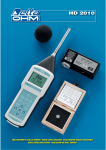
1. Microphone.
2. Preamplifier.
3. Input/Output TRIGGER connector (Jack stereo ∅ 3.5mm).
4. Symbol showing measurement status: RUN, STOP, PAUSE, RECORDING or HOLD.
5. Keypad LEFT key: in graphic mode, it moves the selected cursor towards lower values.
6. Keypad CURSOR key: in graphic mode, it allows to select one or both of the two cursors.
7. HOLD key: it temporarily stops display updating.
8. ALPHA key: combined with other keys it allows to enter alphanumeric strings.
9. MENU key: it activates the different configuration menus of the instrument.
10. REC key (recording): combined with START/STOP/RESET, it activates the continuous data
recording on memory (data logging). When pressed for at least 2 seconds, the displayed data
can be stored in memory as a single record; alternatively, the Auto-Store mode can be activated.
11. PAUSE/CONTINUE key: pauses integrated measurements. From PAUSE mode, integrated
measurements can be resumed by pressing the same key. In PAUSE mode, press
START/STOP/RESET to reset measurements.
12. SELECT key: enables modification mode of displayed parameters by selecting them in sequence.
13. ENTER key. It confirms the entered data or edited parameters.
14. LEFT key: in the menu, it is used when editing parameters with attribute. In graphic mode, it
reduces the vertical scale.
15. M12 connector for multi-standard serial port, RS232C and USB.
16. Auxiliary power supply connector.
17. DC output connector (∅ 2.5mm jack)..
18. DOWN key: in the menu, it selects the next line or decreases the selected parameter. In graphic
mode, it increases the vertical scale levels; the graph is shifted downwards.
19. RIGHT key: in the menu, it is used when editing parameters with attribute. In graphic mode it
extends the vertical scale.
20. MODE key : Selects in circular order the instrument’s different view modes, from the display
of 5 channels in numeric format, to the time profile, to the octave and third octave spectrum
(“Third Octave” option), to the narrow band spectrum (“FFT” option) and to the statistics
screens.
21. UP key: in the menu, it selects the previous line or increases the selected parameter. In graphic
mode, it decreases the vertical scale levels; the graph is shifted upwards.
22. START/STOP/RESET key: when pressed in STOP mode, it starts the measurements (RUN
mode). In RUN mode, it stops the measurements. When pressed in PAUSE mode, it resets the
integrated measurements, such as Leq, SEL, MAX/MIN levels, etc.
23. PROG key: activates the program selection mode.
24. PRINT key: transfers the displayed data to the RS232 serial port. When pressed for more than 3
seconds, it enables the continuous printing (Monitor). Monitoring will be stopped by pressing
the key once more.
25. ON/OFF key. turns the instrument on and off.
26. Keypad RIGHT key: in graphic mode, it moves the selected cursor towards higher values.
27. Battery symbol: indicates the battery level. The more the symbol is empty, the more the battery
has run down.
28. Un-weighted LINE input or output connector (3.5mm ∅ jack).
29. Preamplifier or extension cable connector.
- 3
-
CONNECTOR FUNCTION
The instrument is equipped with six connectors: one in front, two to the side and three at the bottom. The figure on page 2 shows:
n.3 -
Connector for input/output digital TRIGGER (jack stereo ∅ 3.5mm). TRGOUT output can
be enabled using menu function MENU >> Instrument >> Input/Output >> TRGOUT
Source. Input TRGIN can be selected for event trigger using the parameter MENU >> Trigger >> Source.
TRGOUT
GND
TRGIN
Fig. 1 - TRIGGER stereo connector.
n.15 - M12 connector for RS232C multi-standard serial port and USB. For the connection to a
PC’s RS232 port you have to use the dedicated serial null-modem cable (code HD2110RS),
fitted with a 9-pole female connector. As alternative the sound level meter can be connected
to a PC USB port by using the dedicated cable (HD2110USB), fitted with type A USB connector.
n.16 - Male connector for external power supply (∅ 5.5mm-2.1mm socket). It requires a
9…12Vdc/300mA power supply. The positive (pole) power supply must be connected to the
central pin.
n.17 - Jack type socket (∅ 2.5 mm) for A weighted analog (DC) output and Fast time constant, refreshed 8 times per second.
n.28 - Jack (∅ 3.5 mm) for the analogue input/output (LINE) located on the right side of the conical part/detail: the jack can be enabled to work as instrument input through a menu specific
item (MENU >> Instrument >> Input/Output >> Input); otherwise, it operates as an nonweighted analogue output.
n.29 - 8-pole DIN connector for preamplifier or extension cable. The connector, located on the instrument front face, has a positioning notch and a screw ring nut to ensure proper locking.
- 4
-
CERTIFICATO DI CONFORMITÀ DEL COSTRUTTORE
MANUFACTURER’S CERTIFICATE OF CONFORMITY
rilasciato da
issued by
DELTA OHM SRL
DATA
DATE
STRUMENTI DI MISURA
2012/06/13
Si certifica che gli strumenti sotto riportati hanno superato positivamente tutti i test
di produzione e sono conformi alle specifiche, valide alla data del test, riportate nella documentazione tecnica.
We certify that below mentioned instruments have been tested and passed all production
tests, confirming compliance with the manufacturer's published specification at the date of
the test.
Le misure effettuate presso un Laboratorio di Taratura Accredia sono garantite da
una catena di riferibilità ininterrotta, che ha origine dalla taratura dei campioni di
prima linea del Laboratorio presso l’istituto metrologico nazionale.
Measurements performed in an Accredia Calibration Laboratory are guaranteed by a uninterrupted reference chain which source is the calibration of the Laboratory first line standards
at the national metrological institute.
Tipo Prodotto:
Product Type:
Integrating Sound Level Meter
Nome Prodotto:
Product Name:
HD2110L
DELTA OHM SRL
35030 Caselle di Selvazzano (PD) Italy
Via Marconi, 5
Tel. +39.0498977150 r.a. - Telefax +39.049635596
Cod. Fisc./P.Iva IT03363960281 - N.Mecc. PD044279
R.E.A. 306030 - ISC. Reg. Soc. 68037/1998
- 5
-
INTRODUCTION
L’HD2110L is an handheld integrating sound level meter performing either spectral or statistical analysis. The instrument is designed to deliver maximum performance in the analysis of acoustic phenomena with particular attention to regulations on environmental noise and building acoustics. Attention has been paid to the possibility to adapt the instrument’s functions
to the legislation and to meet the needs of its users. It’s possible to integrate the sound level meter at
any time with options to extend the applications; the firmware can be updated directly by the
user using the supplied NoiseStudio software.
HD2110L meets type 1 specifications according to IEC 61672-1 2002 and IEC 60651 , IEC 60804
standards. Compliance with IEC 61672-1 has been verified by INRIM primary metrological Institute (ref. certificate no.37035-01C).
The constant percentage bandwidth filters meet the specifications of IEC 61260 Class 0 and microphone meets IEC 61094-4.
HD2110L is an integrating sound level meter suitable for the following applications:
•
•
•
•
•
•
•
•
•
•
Environmental noise levels evaluation,
noise monitoring with noise events capture and analysis,
spectral analysis in octave bands from 16Hz to 16kHz,
complete statistical analysis with percentile levels calculation from L1 to L99
measurement in working environments,
selection of Personal Protective Equipment (methods SNR, HML and OBM),
soundproofing and acoustic reclamation,
production quality control,
machine noise measurement,
building and architectural acoustics (with “Reverberation time” option).
By activating the "Third Octave" option the sound level meter also performs the following functions:
• third octave spectral analysis from 16Hz to 20kHz and from 14Hz to 18kHz (center frequency shifted bands),
• measurement of noise pollution with tonal components identification ,
• real time evaluation of spectral components audibility, by comparing with the equal loudness curves,
HD2110L sound level meter can capture the noise time profile with complete freedom on the
choice of time constants or frequency weightings. The sound level meter stores automatically the
sound level multi-descriptor analysis as a tape recorder, with a storage capacity of more than
46 hours at the maximum temporal resolution.
For long-term monitoring of the noise level it’s possible to store at intervals from 1 second to
1 hour, 5 programmable parameters in parallel with full statistics and the average spectrum in octave and optionally third octave bands. With its memory the HD2110L can store multi-parametric
analysis and statistics at 1 minute intervals for more than 46 days.
For long term monitoring it is possible to further increase the storage capacity of the analyzer
using the optional HD2010MC memory card interface. This device is equipped with a Secure Digital Memory Card of 2GB.
With HD2110L sound level meter it’s possible to make measurements with a linearity range
of more than 110dB limited in the lower part of the range only by the inherent noise. For example,
setting the upper limit of the measuring range to 140dB, it’s possible to measure the noise levels
- 6
-
typical of a quiet office with the ability, at the same time, to measure accurately peak levels up to
143dB.
The HD2110L is equipped with a versatile trigger function for the capture of sound events,
with the possibility to filter false events by requiring that the variation of the sound level has a specific duration. For each event, it’s possible to store 5 integrated parameters, the average spectra in
octave or third octave (option "Third Octave") bands, and the noise levels probability distribution
during the event. The storage of event’s parameters does not exclude normal and interval recording. The function of event triggering can be activated also manually using a key or via a hardware external signal sent to the TRGIN input.
The sound level meter can activate an external device using the TRGOUT output in parallel
with data acquisition or the occurrence of sound events.
The advanced features of the analyzer allow the acquisition of multi-descriptors noise profiles
in parallel with report sequences with dedicated parameters, average spectra and full statistical
analysis. Moreover, during recording, the trigger function is able to identify sound events and record their analysis with 5 chosen parameters, average spectrum and statistics, integrated for the
event’s duration.
During data logging are available up to 9 different markers to record specific events and consider them in the profiles post-processing phase.
A timer allows to schedule a delayed acquisition start.
Different recordings can be later recalled from internal memory and displayed on the graphical screen using the “Replay” function that shows the time history of recorded noise levels. The
USB interface high transfer speed, combined with RS232 flexibility, allow fast data transfer from
sound level meter internal memory to PC memory but also to control a modem or a printer. For example, in case the internal memory is not sufficient, that’s the case of long term monitoring, it’s
possible to activate the “Monitor” function. Such function allows to transmit displayed data
through the serial interface, recording them directly on PC memory.
The HD2110L can be fully controlled via a PC using the multi-standard serial interface
(RS232 and USB), using a dedicated communication protocol. Through RS232 serial interface it’s
possible to connect the HD2110L to a PC also by means of a modem.
Together with the logging of the overall noise level profiles, the spectral analysis is carried out
in real time for octave bands and for third octave bands, as an option. The sound level meter calculates the spectrum of the sound signal twice a second and integrates it linearly for up to 99 hours.
The average spectrum or the multi-spectrum profile starting from 1s, are displayed together with an
A, C or Z wideband overall level; this allows a fast comparison between spectrum and overall level.
Moreover the spectrum can be shown both as linear and as A or C frequency weighted, for a fast
evaluation of the different spectral components audibility.
In parallel with overall noise profiles acquisition, is performed the real time spectral analysis,
both in octave and in third octave bands (option “Third Octave”). The noise frequency spectrum is
calculated 2 times per second and linearly integrated for up to 99 hours. Alternatively it’s possible
to perform multi-spectral analysis, both max and min, weighted both exponentially and linearly.
Spectra or multispectral profile starting from 1 second , are displayed in parallel with a wide band
A, C, or Z weighted level allowing a fast comparison between spectrum and wide band level.
Moreover frequency spectrum can be displayed both as un-weighted spectrum and as A or C
weighted, for a fast evaluation of different spectral components audibility.
In addition to standardized bands from 16 Hz to 20 kHz, spectral analysis in third octave
bands (option "Third Octave") can be performed with shifted bands; these filters have center frequencies moved downward by one-sixth octave in a range from 14 Hz to 18 kHz. While viewing the
- 7
-
spectrum in third octave bands it’s possible to activate the function to plot on the display the isophone contours for a fast analysis of spectral components audibility.
As a statistical analyser, the HD2110L samples the sound signal 8 times per second with Afrequency weighting and FAST time constant, and analyses it statistically according to 0.5 dB
classes. Statistical analysis is shown in a graphic form as probability distribution and cumulative
distribution with percentile levels from L1 to L99.
It’s possible to choose the descriptor to sample between LFp, Leq or Lpk with A, C or Z frequency weightings (only C or Z for Lpk).
With the HD2110L sound level meter it’s possible to analyse external audio signals using the
LINE input.
For a later analysis, unweighted LINE output allows to record the sound signal on a tape or directly
on a PC with audio acquisition board.
The calibration can be made either using an acoustic calibrator (type 1 according to IEC
60942) or the built-in reference generator. The electric calibration employs a special preamplifier
and checks the sensitivity of the measuring channel, microphone included. A protected area in the
non-volatile memory, reserved to factory calibration, is used as a reference in the user’s calibrations, allowing to keep instrument drifts under control and preventing the instrument from wrong
calibrations.
The user can check on site the complete sound level meter’s functionality thanks to a diagnostic
program.
The most of instrument damages, including those to the microphone, can be identified thanks
to a complete analysis program that includes a frequency response check of the complete measurement chain composed by microphone, preamplifier and sound level meter. A periodic check using diagnostic programs allows to perform safely acoustic measurements, removing the risk of having to repeat them for a malfunction discovered too late.
The HD2110L sound level meter can perform the measurements required to evaluate workers’
noise exposure (D.L. N.81/2008, UNI 9432/2011 and ISO 9612/ 2011 standards). According to
UNI EN 458, the personal protective equipment can be selected through octave band spectrum
analysis (OBM method) and a comparison of the A and C-weighted equivalent levels that can be
measured simultaneously (SNR method).
If an undesired sound event produces an over-load indication, or simply alters the result of
an integration, its contribution can be excluded using the versatile Back-Erase function. The impulsivity of a noise source is easily evaluated (according to criteria defined in UNI 9432 standard)
measuring the A weighted equivalent sound pressure level with Impulse time constant (LAeqI).
The cyclic, fluctuating and impulsive noise sources identification is simple thanks to the
powerful recording functions of HD2110L analyser which allows, using a single measurement
setup, to solve the most of situations encountered in working environments. The combination of
powerful measurement and recording functions of HD2110L with the analysis functions of the post
processing Noise Studio (supplied with all sound level meters) software module “Worker’s protection”, allows a fast and efficient management of noise measurements for health and safety evaluations in workplaces.
The HD2110L sound level meter is suitable for sound level monitoring, acoustic mapping, and the
assessment of the acoustic climate with capture and analysis of sound events. When measuring traffic noise near airports, railways and roads, the sound level meter can be used as a multi-parameter
sound recorder, combining spectrum and statistical analyser features. Remote electrical calibrations
and diagnostic tests can be executed using its remote control functions.
- 8
-
The HD2110L sound level is able to perform all measurements prescribed by the regulations
concerning the evaluation of environmental noise. The impulsive events identification is easy,
thanks to the ability to analyze noise profile with parallel FAST, SLOW and IMPULSE time constants. All measurement parameters can be stored for a later analysis.
With “third octave” option it’s easy to identify tonal components; spectrum of minimum
level, evaluated with a wideband frequency weighting (Z, C or A), is displayed and stored; the frequency spectrum is calculated both for standard center frequencies from 16Hz to 20KHz and for
non-standard shifted (one-sixth octave) central frequencies from 14Hz to 18KHz Audibility of tonal components can be evaluated in post processing using the Noise Studio PC software or directly
on site thanks to real time function of isophone curves plot implemented in the sound level meter.
The HD2110L, sound level meter, with the “Reverberation Time” options, can perform all
measurements prescribed by the regulations on building acoustics evaluation (ISO 140). The sound
level meter powerful DSP calculates 32 spectra/second, and it can measure reverberation times both
using the sound source interruption and the impulsive source integration technique according to
UNI EN ISO 3382. The HD2110L sound level meter analyses the noise level decays with the Ordinary Least Squares method, simultaneously both by octave from 125Hz to 4KHz and, if option
“Third Octave” is installed, by third octave bands from 100Hz to 12.5KHz according to survey, engineering and precision methods defined in UNI EN ISO 3382-1/2009 and 3382/2008.
The HD2110L can be configured in accordance with different customers’ needs: the available
options can be activated on the new instrument, as well as, later on, when requested by the user. The
provided options are:
“Third Octave” option
Option “Third Octave” adds a double bank of third octave filters from 16 Hz to 20 kHz and
from 14 Hz to 18 KHz (shifted downwards by one-sixth octave) in class 1, according to IEC 61260.
The filter bank works in parallel to all other measurements. The audibility of the different spectrum
components can be evaluated applying A or C frequency weightings or thanks to the isophone
(equal loudness level) curve calculation function supplied with the instrument and available directly
on the sound level meter’s display.
“FFT” option
“FFT” option adds the following functions:
• The linearly integrated level on 1/32s (Leq Short) with frequency weightings A, C or Z is
available for recording.
• In addition to octave bands, real time frequency analysis is performed also in narrow bands
(FFT) on the whole audio range with a variable frequency resolution from 1.5Hz up to
100Hz. Narrow band frequency analysis calculates 2 spectra per second, without any penalty
on the sound level meter dynamics and in parallel with octave and third octave spectra.
“Reverberation Time” option
Through this option the HD2110L can carry out reverberation time measurements according to
the techniques of the sound source interruption and of the impulse response according to EN ISO
3382-2/2008 requirements. This measurement is made simultaneously for octave band from 125 Hz
to 8 kHz and , if option is installed, for third octave band from 100 Hz to 10 kHz. The sampling interval equals 1/32s and the calculation of EDT, T10, T20 and T30 reverberation times is made
automatically for all bands.
- 9
-
Block Diagrams HD2110L
Fig. 2 - Instrument’s Block Diagrams
The block diagram shows the main elements of the HD2110L sound level meter.
- 10 -
The Microphone
The provided microphone is the condenser type MC21, it is polarized at 200 V and has a ½”
standard diameter. The frequency response in free field is flat throughout the whole audio range.
The MC21 microphone meets the requirements of IEC 61094-4 international standard for WS2F
type.
Optionally it’s possible to install other types of microphones having the same electro-mechanical
specifications than MC21 and complying with the IEC 61094-4 standard, like for example the
MC22 microphone with optimized diffuse field frequency response:
For more details and specifications on microphones available for HD2110L sound level meter,
please refer to the specific manuals
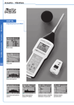
The Outdoor Microphone Unit HD WME
The HD WME microphone unit is suitable for long lasting outdoor monitoring, even in a fixed
unattended location. The unit is adequately protected from rain and wind and the heated preamplifier together with the protective membrane coating of the microphone capsule provide stability of acoustic parameters over time and allow you to make measurements over a wide range of
environmental conditions.
The Delta Ohm sound level meter preamplifier matched with the outdoor microphone unit is
equipped with a circuit for electrical calibration of the preamplifier - microphone chain, a technique that uses a charge distribution.
The frequency response of the unit in free field meets the specifications of class 1 according to
IEC 61672 (and IEC60651). The microphone unit
HD WME must always be positioned vertically
to allow the anti-rain to perform its function and
can be used both to detect the noise from the air and
the ground. The Delta Ohm sound level meters perform spectral corrections to the measures to ensure
tolerances in accordance with the IEC61672 class 1
in every situation.
The easiness of disassembly and reassembly of the
unit allows to perform periodic testing of the electro- acoustic characteristics the same way as a standard measurement microphone, using a standard
calibrator for ½" microphone.
The unit consists of a central body and the following parts:
- 11 -
HD SAV3: windscreen (3)
HD WME1: anti-bird spike (4)
HD WME2: rain shield (2)
HD WME3: stainless steel holder (1)
Microphone capsule with optimized frequency response for “free field”:
Microphone preamplifier:
HD 2110PW (or HD2110PEW): heated preamplifier for 200V polarized or electret
microphones, with CTC calibrator and differential driver.
HD 2110PEW: heated preamplifier for prepolarized microphones, with CTC calibrator and differential driver
Connection cable 5m (other lengths up to 100m available on request).
For more details on the outdoor unit HDWME, refer to the chapters dedicated to calibration on
page 62 and its assembly and disassembly in appendix on page 178.
The Preamplifier
The preamplifier amplifies the weak signal provided by the microphone. The preamplifier has a
gain selectable between 0 and 10 dB and is supplied with a charge partition calibration device
which allows to measure the frequency response of the whole amplification chain, microphone
included (diagram described on page 64).
A special output driver allows to transmit the microphone signal via a cable up to a 100 m distance. The preamplifier of HD2110L can measure noises up to 140dB with a flat frequency response up to 40 kHz.
The following preamplifiers are available:
HD2110P: preamplifier with standard ½ connector for 200V polarized microphones. This
preamplifier, equipped with CTC calibration device for electric calibration, can be directly
connected to HD2110L sound level meter or connected using the extension cable up to 100m
length.
HD2110PE: preamplifier similar to HD2110P but suited for pre-polarized (Electret) microphones.
- 12 -
HD2110PW: heated preamplifier with standard ½ connector for 200V polarized microphones
and cable driver. This preamplifier, equipped with CTC calibration device for electric calibration, can be directly connected to HD2110L sound level meter or connected using the 5mt
extension cable (other lengths on request).
HD2110PEW: preamplifier similar to HD2110PW but suited for pre-polarized (Electret) microphones.
The Instrument
The signal of the preamplifier comes to the instrument receiver and its output is sent to the LINE
connector and to the A/D converter input. The instrument can be set to use the LINE channel in
place of the signal coming from the preamplifier.
The analogue signal is converted into numeric format at 25 bit from the A/D. The exceptional
resolution of the converter, which covers a 140 dB range, allows to keep a high resolution over a
measuring range of about 110 dB, where the digitization error is negligible.
The levels either wideband (A, C and Z) or with constant percentage bandwidth (both octave
and, optionally, third octave) are calculated in parallel in the DSP. Peak (C and Z) levels are also
calculated. The levels calculated by the DSP are transmitted to the microprocessor for further
processing, ready to be displayed, stored and printed.
The microprocessor controls all the instrument processes: management of the electrical calibrator, Flash memory, display, keyboard and multi-standard serial interface (RS232 and USB).
- 13 -
DESCRIPTION OF DISPLAY MODES
The HD2110L measures simultaneously 5 selectable parameters (statistic ones too) at a fixed
frequency corresponding to 2 measurements/s; moreover, it measures a selectable parameter at intervals programmable between 1/8s and 1h; at the same time it calculates the octave and third octave ( “Third Octave” option) band spectra, with a maximum frequency of 2 spectra/s and, with option, narrow band FFT spectrum. As statistical analyzer it calculates the probability distribution and
percentiles. To be able to display all these data, the HD2110L provides 7 different display modes as
shown in the figures below.
Tint=10s 01:08:25
130
20
Leq
LFp
LImx
LSp
Lpk
LFmx 00:02:05
dBC
56.9
52.5 dBA
90
20/
83.8 dBA
50.3 dBA
78.5 dBC
10
1/2s
dBA
Fig. 3 - SLM
Fig. 4 - Time profile
MLT 10m 126 05:38
MLT 5s 026 00:03
90
70
20/
20/
10
LIN
1K
-10
8K L
FAST
Fig. 5 - Octaves
1K
8K A
Fig. 6 - Third of octaves (option)
Fig. 7 - FFT (option)
Fig. 8 - Probability Distribution
Fig. 9 - Percentiles
- 14 -
In order to jump from a screen page to the next one press MODE at any time. The display
will show in a sequence first the SLM screen with 5 measuring parameters in numeric format, the
Profile screen with the time trend of a parameter, the screens of Octave and Third Octave (option), with the octave (from 16Hz to 16 kHz) and third octave spectra (from 16 Hz to 20 kHz), respectively, the FFT narrow band screen (option), the distribution of probability and percentiles
screens. Upon power on, the sound level meter displays the SLM screen.
The display of the OCTAVE and THIRD OCTAVE screens can be disabled using the relevant menu parameters (Menu >> Spectrum Analyzer >> Display…).
Also the PROBABILITIES and PERCENTILES screens can be disabled using the menu parameter
Menu >> Statistical Analyzer >> Display Statistics (see paragraph “DESCRIPTION OF THE
MENU FUNCTIONS” on page 49).
on progress
overload indicator
Some indications are shown in all modes. They are
memory
(see the figure on the right):
RUN
Measurement status indicator,
PAUSE
Overload indicator,
REC
Battery level indicator.
STOP
20
The first symbol in the left corner at the top shows
H HOLD
the measurement status of the sound level meter.
Leq
W WarmUp
RUN: the instrument is measuring.
P Print
PAUSE: the calculation of integrated measurements
M Monitor
and the recording of measurement have been susR Replay
pended. Instantaneous parameters are still being
measured and displayed.
REC: the instrument is measuring and recording.
Fig. 10
STOP: the instrument is not making any measurement.
HOLD: the calculation of integrated measurements has come to the end of set integration interval,
or HOLD was pressed.
W (Warm Up): signal that appears upon the instrument power on and that disappears after approximately 1 minute. It warns the user to wait the time necessary to the instrument to reach steady
conditions, in order to ensure best performances.
P (Print): indicates that printing is in progress.
M (Monitor): indicates (flashing) that continuous data printing has been started.
R (Replay): appears (flashing) when the “Memory Navigator” program is in use, to view a file
saved in the instrument memory (see page 57).
Just on the right of the symbol indicating the logging mode, there is the symbol showing a
possible overload. An arrow directed upwards indicates that the input level has exceeded the
maximum measurable level.
The maximum measurable level corresponding to the selected measurement range is given in the
technical specifications (see page 112). Using an appropriate parameter (MENU >> Instrument >>
Measurement >> Overload Level) you can program the maximum measurable limit at lower levels
(see page.112).
An empty arrow indicates that the limit has been exceeded, while a full arrow indicates that the
overload is in progress. No sub-range indication is needed, because the minimum measurable level
is limited only by the electrical noise, as shown in the technical specifications.
The integration time Tint, programmable between 1s and 99h, is displayed to the right of the
overload indicator. When the integration mode is set on MULT, the “Tint” symbol on the SLM will
flash (see the “DESCRIPTION OF THE DIFFERENT INTEGRATION MODES” chapter on
page 39).
- 15 -
In the right corner at the top, there is the battery symbol. The more the symbol is empty, the
more the battery has run down. When the instrument autonomy reaches 10%, corresponding to
about 30 minutes, the battery symbol will start flashing. A protection device prevents the instrument
from making measurements with insufficient battery levels and automatically switches off the instrument when the battery level is at the minimum.
The battery level, expressed in percentage, is visible in the menu main screen page and in the
program page; press MENU and PROG to access them. To jump back to the measurement screen,
press MENU and PROG again.
Pressing SELECT, you will select in sequence the parameters relevant to the displayed page.
While the selected parameter flashes, you can change it with the UP and DOWN keys. Press ENTER to quit the selection mode (automatic exit after 10s).
In graphic display mode, use the UP, DOWN, LEFT and RIGHT keys to change the vertical
scale parameters. The LEFT and RIGHT keys reduce and expand the vertical scale, while the UP
and DOWN keys decrease and increase the levels of the vertical scale; the graph is so shifted upwards or downwards, respectively.
- 16 -
SLM (SOUND LEVEL METER) MODE
This is the display mode upon power on.
Five parameters (selectable among the following ones) can be displayed simultaneously:
• Instantaneous acoustic broadband levels such as Lp, Leq(Short) and Lpk, either with wideband
frequency weightings or by octave or third octave bands. The pressure levels displayed are the
maximum levels reached every 0.5s
• Integrated acoustic broadband levels, such as Lpmax, Leq , LIeq and Lpkmax, either with wideband
frequency weightings or with octave or third octave bands, updated every 0.5s
• Up to 4 percentile levels selectable between L1 and L99
• Sound exposure level
• Average level with 4 dB exchange factor
• Average level with 5 dB exchange factor
• Daily personal exposure level
• Dose and daily Dose with programmable Exchange Rate, Criterion and Threshold Levels
• Overload Time (in %)
The display is updated every 0.5 seconds.
Data recording varies depending on the selected integration mode (single or multi) and on the activation or not of Auto-Store function as described in the following table (see chapter DESCRIPTION OF THE DIFFERENT INTEGRATION MODES on page 39).
Integration
Auto-Store: OFF
Auto-Store: ON
SINGLE
Recording twice per second enabled
by Recording menu. Automatic Stop
at the end of the set integration interval.
Automatic recording of SLM page together with OCTAVE and (optional)
THIRD OCTAVE spectra in AVR mode
at the end of the set integration interval.
MULTIPLE
Recording twice per second enabled
by Recording menu. Automatic reset
of integrated levels at every integration interval.
Automatic recording of SLM page together with OCTAVE and (optional)
THIRD OCTAVE spectra in AVR mode
at intervals equal to the set integration
time. At the beginning of each period, integrated levels and spectra are set to zero.
- 17 -
Display Description
Left at the top of the display there are the recording status symbol and the overload indicator
(described at the beginning of this chapter). In the midst there is the integration interval and on the
right the acquisition time (hours:minutes:seconds). When the integration mode is set on MULT
(MENU >> Instrument >> Measurements >> Integr.Mode: MULT), the “Tint” symbol flashes. The
battery symbol is in the right corner, indicating battery level.
Integration interval
Minimum level
Displayed parameters
Acquisition time
Tint=10s 01:08:25
20
130
Leq
LFp
LImx
LSp
Lpk
dBC
56.9
52.5 dBA
Maximum level
Bar showing
istantaneous level
83.8 dBA
50.3 dBA
78.5 dBC
Fig. 11 - Description of the display in SLM mode
The “analogue bar” shows the sound pressure instantaneous level in a 110dB interval.
Big in the centre of the display is the main measurement parameter, followed by four further parameters. All displayed parameters can be freely selectable among the available ones. There are no
restrictions in the selection of frequency weightings. Measuring parameters are displayed with a
shortened label, followed by the numerical value, by the unit of measurement, and, when necessary,
by the frequency weighting. The correspondence between the label and the effective parameter is to
be found in appendix on page 144.
Integrated parameters like Leq (and Lmax or Lmin), which imply the time increase of the
sampled sound level, are displayed with a series of dashes (- - - -) until the parameter remains lower
than the minimum measurable level.
Before starting a new logging, the sound level meter automatically resets all measurements. If
the multiple integration mode is enabled (MENU >> Instrument >> Measurement >> Integration
Mode: MULT), integrated levels will be automatically set to zero at regular intervals equal to the
set integration time Tint.
Selecting parameters
Some measuring parameters (integration interval, measuring range and the five parameters)
can be changed directly via the SLM screen.
Pressing SELECT you choose the different parameters in sequence. While the selected parameter
flashes, you can change it with the UP and DOWN keys.
If a parameter with attribute is selected, like, for example, LFp (FAST weighted pressure
level) in Fig. 11, the relative frequency weighting will also flash (A in the example). In this case,
pressing UP and DOWN, you can modify the selected parameter without changing the attribute; for
example, if you press DOWN, you can go from LFp A weighted to LSp A weighted.
Pressing RIGHT you’ll jump to the attribute selection, which will be the only one to flash. Use then
the UP and DOWN keys to change the attribute. For example, if you press UP, you can go from A
weighted LSp to Z weighted LSp.
Pressing LEFT while selecting the attribute, you return to parameter selection.
Pressing SELECT let you choose the next parameter; pressing ENTER, or automatically after
approximately 10s, will let you exit the selection mode.
- 18 -
Also the integration mode (see page. 39) can be set using the LEFT and RIGHT keys: press
SELECT to choose the integration interval. When the integration interval numeric value flashes
press RIGHT to set the multiple integration mode or LEFT to set the single integration mode. When
the integration mode is set on MULT, the “Tint” symbol flashes.
Parameters can be modified only when the instrument is in STOP mode: if you try to
make changes to any of the parameters while the instrument is in a status other than STOP, you will
be asked to stop the measurement in progress: pressing YES will stop recording and will allow you
to go on modifying parameters; pressing NO recording will continue without interruption.
The above settings can be made through the instrument configuration menus. See a detailed
description on page 49.
Back-Erase Function (data exclusion)
To stop a measurement in progress when recording, press the PAUSE/CONTINUE key.
All data logged until the moment key was pressed are used for calculation of integrated parameters.
However, there are some cases when it is useful to clear the measurements recorded just before
pressing PAUSE, for example, because they were caused by unexpected events and not characterizing the sound being examined.
During measurement, press PAUSE/CONTINUE: integrated measurements update will be interrupted. At this point, press the LEFT arrow to delete the last recorded data.
The integration time value will be temporarily replaced by the word “Clear” followed by the
time interval (in seconds) to be deleted.
Use the LEFT and RIGHT keys to increase or decrease the erase interval. Displayed integrated parameters change accordingly, allowing to choose the erase time depending on the effective
need. When pressing PAUSE/CONTINUE again, measurement will start again and the integrated
parameters will have been removed from the selected interval.
The erase maximum time, divided into 5 steps, is set from menu: MENU >> Instrument >>
Measurement >> Max Back-Erase. Settable values are: 5, 10, 30 or 60 seconds, with 1s, 2s, 6s or
12s steps, respectively.
- 19 -
TIME PROFILE MODE
This display mode presents the time profile of a selectable parameter. You can display a parameter out of the integrated one, like Lpmax, Lpmin, Leq and Lpkmax, either with wideband frequency
weightings or with octave or third octave bands (option “Third Octave”).
Integration and sampling time is programmable between 1/8s and 1h (from 1/2s to 1h for the levels
with constant percentage bandwidth filters); the last 100 measured samples are displayed.
The HD2110L sound level meter calculates the sound level, weighted A, C or Z, 128 times
per second. The Profile screen gives the best time resolution by providing up to 8 values per second,
exponentially (i.e. LFmx) and linearly (i.e. Leq) weighted. For example, when you choose to display a profile of the maximum FAST pressure level (LFmx), a flow of 128 samples per second of
the FAST pressure level is examined, and the maximum level is displayed at regular intervals according to the set profile time.
Pressing HOLD, the display update will be stopped; however, the instrument continues measuring and pressing HOLD again will restart display updating.
The HOLD status does not affect neither Monitor (continuous printing) nor recording operations. When the continuous recording is activated with the single integration mode, the integration
time acts like a timer for data acquisition, stopping automatically the measurement when the time is
elapsed.
This screen-page is not recorded in the Auto-Store mode.
Display Description
Acquisition time
Displayed parameters
Leq
Maximum level
90
Scale factor
20/
Minimum level
00:00:10.0
Analogic bar
10
dBA
1/8s
Sampling interval
Weighting
Fig. 12 - Description of the Profile mode display
For example, Fig. 12 shows the time profile of A weighted Leq with a 0.125s sampling interval. Selecting LFmax as parameter and 1s as sampling time, you can, for example, view the time
profile of the FAST weighted maximum pressure level calculated every second.
The integration interval is shown in the left corner at the bottom of the display. Always at the bottom, in the centre, the display shows the measurement unit and the frequency weighting of the
measuring parameter.
The amplitude of the vertical scale of the displayed graph corresponds to 5 divisions. The amplitude
of each division is called “scale factor” of the graph and appears in the middle of the vertical axis.
Using the RIGHT (zoom +) and LEFT (zoom -) keys, this parameter is selectable in real time
among 20dB, 10dB or 5dB by division).
- 20 -
Use the UP and DOWN arrows to set the graph full scale with steps equal to the selected scale
factor, starting from the instrument full scale1. In this way, the graph can be shifted UP or DOWN,
depending on the key you have pressed.
An “analogue” bar indicator on the display right side provides the non-weighted instantaneous
level of the input sound pressure level, as for the SLM mode bar.
Some parameters can be modified without accessing the menus, but simply using the SELECT key, the four arrows (UP, DOWN, LEFT and RIGHT) and ENTER key. They are the displayed parameter, its frequency weighting and the profile time (for more details, see the paragraph
"Selecting parameters" on page 18)
In this display mode, Recording and Monitor functions work as in the SLM mode: the only
difference is that the time interval with which data are recorded or sent to the serial interface is programmable and corresponds to the sampling interval, except for 1/8s and 1/4s sampling times,
where 4 values and 2 values every 0.5s are respectively recorded or sent to the interface.
The integration mode and the Auto-Store function do not influence this screen recording functioning.
The sound level displayed on this screen can be used as source for the event trigger (see paragraph “EVENT TRIGGER FUNCTION” on page 38).
Using the Cursors
To activate cursors on the graph, press CURSOR on the keypad. If you press CURSOR repeatedly, either L1 or L2 cursor, or both ΔL cursors in “tracking” will be activated in succession:
the selected cursor will flash. Use the LEFT and RIGHT arrows on the keypad to move the selected
cursor on the graph.
The second line at the top of the display shows the level of the measuring parameter and the
time indicated by the active cursor or the time interval and the L1-L2 level difference between the
two cursors when they are both active.
The parameter level being lower than the minimum measurable level is indicated by a series
of dashes (- - - -)
Press CURSOR again to disable the cursors.
1
The instrument full scale is determined by the selection of the input gain by choosing from the menu: MENU >> Instrument >> Measurements >> Input gain.
- 21 -
SPECTRUM MODE (BY OCTAVE AND THIRD OCTAVE BANDS)
The spectrum analyzer operation mode allows the visualization of frequency spectrum by
octave bands from 16Hz up to 16kHz and by third octave bands from 16Hz to 20kHz (“Third Octave” option). The spectral analysis is carried out and possibly stored on unweighted samples (Z)
while the display can also be A or C weighted, for a fast evaluation of audibility of different spectral components.
The spectrum by octave bands or by third octave bands is combined, for possible comparisons, with a wideband level that can be set as A, C or Z weighted. The selected wideband weighting
is called “auxiliary weighting” and plays an active role in the maximum or minimum multispectrum analysis.
The spectrum recording mode can be chosen between:
• Linear averaging (AVR) with integration times from 1s up to 99 hours.
• Multi-spectrum (MLT), even maximum (MAX) or minimum (MIN) with programmable partial integration interval from 0.5s to 1h, either linearly (LIN) or exponentially (EXP) averaged
with FAST (0.125 s) or SLOW weights (1 s).
The average spectrum (AVR) is linearly integrated band by band throughout the integration time
shared with the SLM mode (from 1s to 99h).
If integration is performed in single mode (MENU >> Instrument >> Measurement >> Integration Mode: SINGLE), the instrument will automatically switch into the HOLD mode when
reaching the set integration time, allowing to check the result and eventually print or store it. Press
HOLD to continue with the display update.
If the continuous recording is activated (by pressing simultaneously REC and START keys),
the integration time will act like a timer, stopping automatically the measurement when the time
Tint is elapsed.
If the acquisition mode is AVR and the integration is in multiple mode (MENU >> Instrument
>> Measurement >> Integration Mode: MULT), the instrument will automatically reset the levels at
the end of the programmed integration time, starting a new integration cycle (see the
“DESCRIPTION OF THE DIFFERENT INTEGRATION MODES” on page 39). When AutoStore function is active (see “THE RECORD FUNCTION” on page 43), spectra acquisition is
automatically set to linear averaging (AVR).
The multi-spectrum analysis (MLT) allows to measure a continuous sequence of spectra,
linearly or exponentially averaged over the programmed profile time (from 0.5s to 1h). While linearly averaged spectra provide the equivalent levels for each band on the profile time, the exponentially averaged spectra are calculated starting from the maximum weighted FAST or SLOW spectra,
calculated every 0.5s. Therefore, while the linearly averaged multi-spectrum (MLT) analysis consists of a sequence of spectra giving the equivalent levels by band, integrated on the programmed
profile time, the exponentially averaged multi-spectrum (MLT) analysis, instead, consists of a sequence of instantaneous spectra displayed at intervals corresponding to the programmed profile
time.
The maximum or minimum (MAX or MIN) multi-spectrum analysis can be also carried out,
where the spectra of the maximum or minimum levels over the set profile time will be measured. In
this mode, displayed spectra depends on the trend of the programmed wideband auxiliary level. The
instrument will display, at intervals corresponding to the profile time, the spectra corresponding to
the maximum or minimum level measured in the programmed interval, with a 0.5s resolution. The
MAX or MIN multi-spectrum analysis, linearly weighted, consists of a continuous sequence of
spectra composed of equivalent levels (integrated on 0,5s) for each band corresponding to the
maximum or minimum equivalent level, measured every 0.5s, with the selected auxiliary weighting.
- 22 -
MULTIPLE
Integration
SINGLE
The (MAX or MIN) multi-spectrum analysis, exponentially weighted, consists of a continuous sequence of spectra corresponding to the maximum or minimum instantaneous level, weighted
FAST or SLOW, measured every 0.5s, with the selected auxiliary frequency weighting.
Spectral analysis, normally unweighted, can be also carried out using A or C frequency
weightings. A or C frequency weighted analysis can be used to evaluate the audibility of different
spectral components. Some parameters, can be modified without accessing the menus, but simply
using the SELECT, the four arrows (UP, DOWN, LEFT and RIGHT) and ENTER keys; by pressing repeatedly the SELECT key can be selected in a sequence: the type of analysis, the integration
or profile time, the average type, the broad-band auxiliary weighting, the A, C or Z spectrum frequency weighting and the temporal [linear (Leq) or exponential FAST or SLOW] average mode
(for more details, see "Selecting parameters" on page 18)
In this display mode, the Continuous Recording and Monitor functions work as in the SLM
mode. The only difference concerns the multi-spectrum, also maximum or minimum (MLT, MAX
and MIN) analysis, where the time interval with which data are recorded, or sent to the serial interface, equals the programmed profile time.
The integration mode and the Auto-Store function change the recording functioning as described in the table below (see the chapter “DESCRIPTION OF THE DIFFERENT INTEGRATION MODES” on page 39).
Auto-Store: OFF
Auto-Store: ON
Recording of OCTAVE and T.OCTAVE spectra, enabled by Recording menu. The recording
interval is equal to the set spectrum profile time
or to 0.5s in AVR mode. Automatic Stop at the
end of the set integration interval.
Only AVR mode.
Automatic recording of OCTAVE
and THIRD OCTAVE spectra (together with SLM) at the end of the
set integration interval.
Recording of OCTAVE and T.OCTAVE spectra, enabled by Recording menu. The recording
interval is equal to the set spectrum profile time
or to 0.5s in AVR mode. When set in AVR
mode spectra are cleared at the beginning of
every integration period.
Only AVR mode.
Automatic recording of OCTAVE
and THIRD OCTAVE spectra (together with SLM) at intervals
equals to the set integration time.
Integrated levels are cleared at the
beginning of each integration period.
Display Description
The display upper line changes according to the selected update mode: whether multispectrum (MLT, MIN or MAX) or average weighted (AVR).
In the first case, after the recording status symbol and the overload indicator, the display
shows the graph updating mode (MLT, MAX or MIN), the partial integration time, the number of
spectra already displayed and the partial integration time of the current spectrum.
If the update mode is the average weighted one (AVR), the display will show the integration
interval (parameter shared with the SLM display mode) and, on the right, the current recording
time.
The values on the left side of the graph are: the full scale, the scale factor and the scale beginning. The amplitude of the vertical scale of the displayed graph corresponds to 5 divisions. The amplitude of each division is called “scale factor” of the graph and appears in the middle of the vertical
- 23 -
axis. Using the RIGHT (zoom +) and LEFT (zoom -) keys, this parameter is selectable in real time
among 20dB, 10dB or 5dB by division.
Use the UP and DOWN arrows to set the graph full scale with steps equal to the selected scale
factor, starting from the instrument full scale2. In this way, the graph can be shifted UP or DOWN
according to the pressed key.
A bar on the display right side shows the wideband level, weighted Z, C or A, as selected. The
applied frequency weighting is shown under the bar.
In the display lower left part it’s shown the spectrum frequency weighting (A, C or Z user
selectable), the time average mode, linear (Leq) or exponential with FAST or SLOW time constants.
Fig. 13 - Display Description in Octave and Third Octave mode
Using cursors and isophone curves
To activate cursors on the graph, press CURSOR on the keypad. If you press CURSOR repeatedly, either L1 or L2 cursor, or both L cursors in “tracking” will be activated in succession: the
selected cursor will flash. Use the LEFT and RIGHT arrows on the keypad to move the selected
cursor on the graph.
The display second line shows level and central frequency of the filter indicated by the active
cursor, or the level difference between the two cursors when they are both active.
2
The instrument full scale is determined by the selection of the input gain by choosing from the menu: MENU >> Instrument >> Measurements >> Input gain.
- 24 -
The level is shown in dB for unweighted (Z) spectra while it’s in dBA or dBC for A and C
weighted spectra respectively.
In the octave and third octave spectrum mode, cursors can be also positioned on the bar representing the wideband channel.
In the AVR and MLT modes with linear average, filters having a level lower than the minimum measurable are indicated by the cursor with a series of dashes (- - - -).
If you press and hold down the CURSOR key for at least 2 seconds, while the unweighted (Z)
spectrum by third octave is displayed, the real time tracing of isophone curves (according to
ISO226/2003) will be activated.
MIN 30s 005 30:0
L1 68dB 88
70
10/
30
FAST
900
9K A
Fig. 14 - Isophone curves
Press CURSOR again and hold it down for at least 2 seconds to disable the isophone tracing.
When the isophone curve is active, the cursors perform different functions with respect to the
standard display described above. The L1 cursor is combined with the isophone tracing, L2 holds
standard functions, ΔL presents two values: the first one represents, as in the standard case, L1-L2
difference; the second one provides the difference between the isophone and L2.
The isophone is calculated to have the same level of the current spectrum in correspondence
with the band selected by L1 cursor. Activating the ΔL function, you can, using the LEFT and
RIGHT arrows of the keypad, move the L2 cursor to check numerically if the band corresponding to
L1 is the most “audible” of the spectrum, verifying that the isophone passing through the level corresponding to the L1 cursor is always higher than or equal to the other levels of the spectrum.
If the L1 cursor is positioned on the bands with 16 Hz, 16 kHz and 20 kHz central frequencies,
where isophone curves are not defined, or if the level of the selected band is lower than the minimum audible, the minimum audibility isophone (MAF) will be displayed.
The isophone display is not available for A or C weighted spectra
THIRD OCTAVE FILTERS SHIFTED BY HALF BAND (“THIRD OCTAVE” OPTION)
The spectrum by third octave band provides, in rather all cases, all information necessary to
classify sound sources. In some cases, however, this type of spectrum can provide wrong indications, when not properly interpreted. The most frequent example is the analysis of a sound source
emitting a “pure” tone, that is a noise with an energy located in a limited area of the spectrum,
around a precise frequency.
This source is correctly classified when the tone is located far from crossing frequencies between adjacent third octave bands; in this case the band of the spectrum containing the frequency of
the pure tone can be easily identified since it is higher than the adjacent average and provides the
sound level of the tone.
If, on the contrary, the frequency of the tone emitted by the source is located exactly at the
crossing of the two adjacent bands, the two bands will show levels higher than the surrounding average value, each of them with a level 3 dB lower than the “true” level of the tone.
- 25 -
The HD2110L sound level meter can be programmed to calculate the third octave band spectrum with central frequencies shifted by half band (1/6th octave) with respect to standard values, in
such a way that “shifted” bands are exactly in the middle of crossing frequencies of “standard”
bands.
From the comparison between “standard” and “shifted” spectra, you can determine the presence of
a pure tone with any characteristic frequency and measure its level.
MIN 30s 003 30:0
MIN 30s 005 30:0
70
70
10/
10/
30
30
FAST
Fig. 15
1K
8K A
FAST
900
9K A
Fig. 16
In Fig. 15 a pure tone at about 70Hz frequency is within the crossing between standard bands with
central frequencies of 63Hz and 80Hz.
The spectrum of Fig. 16 shows the pure tone, using 1/6th octave shifted bands from 14 Hz to 18
kHz.
Follow this instructions to activate the “shifted” spectrum: from the menu, select Spectrum
analyzer (MENU >> Spectrum analyzer >> ENTER key). Select “1/2 Band Shift” and set it ON:
press ENTER to confirm and the following screen will appear.
WARNING !
Automatic Power Off
Change effective
after power on.
CONTINUE
Press CONTINUE and the instrument will switch off. Upon the next power on, a message
will be displayed stating that third octave filters have temporarily been shifted by half a band
downwards. Press CONTINUE to confirm. In this operation mode, the time profile and octave spectrum screens have not been activated, while all the other functions are operative.
Switch the instrument off and then on again to restore its standard working.
- 26 -
MEASUREMENTS WITH THE FFT OPTION
The FFT option provides an additional display mode shown in the following figure
Fig. 17 - FFT
Press MODE at any time to jump from a screen page to the next one: the SLM, PROFILE, OCTAVE, THIRD OCTAVE (“Third Octave” option), FFT (“FFT” option), PROBABILITIES and
PERCENTILES screens will be displayed in this sequence.
The display of FFT screen can be disabled using the relevant menu parameters (Menu >> Spectrum
Analyzer >> Display FFT).
The FFT option adds the narrow band spectral analysis (FFT) and the acquisition of the equivalent
level profile, integrated on intervals equal to 1/32s (Leq Short).
LEQ SHORT AT 1/32s (FFT” OPTION)
The equivalent level integrated every 1/32s with A, C or Z weighting, can be used for a detailed examination of the time profile of sound pulses. This acoustic descriptor, called Leq Short, is
calculated by square integration of the sound pressure every 1/32s.
The Leq Short at 1/32s cannot be displayed by the instrument and is only available for recording. The word Leq Short, short equivalent level, indicates that the level is integrated on a sequence of short intervals, not the whole measurement time. From the Leq Short profile you can calculate the equivalent level on the total and on parts of the measurement time.
A Leq Short parameter can also be selected in the SLM screen. However, the latter is calculated twice per second and therefore corresponds to the square sum of 16 Leq Short values on 1/32s.
From the stored Leq Short profile, calculated 32 times per second, it is also possible to approximate the FAST, SLOW, and IMPULSE levels well. To calculate the sound pressure level with
exponential time constant you need a time profile with a time resolution at least equal to the time
constant. For example, to calculate FAST levels profiles from the Leq Short, you need at least a 1/8
per second time resolution as the FAST time constant. To calculate the IMPULSE profile you need
a Leq Short on lower intervals of 35ms.
In the following figure, as an example, a Leq Short profile is shown, integrated at 1/32s (31.25ms)
intervals, matching a sound pulse composed of 4 sinusoidal cycles at 4kHz with 1ms total duration.
- 27 -
Leq Short Profile
100
90
level [dB]
80
70
60
50
40
30
34
35
36
37
38
39
40
time [s]
Fig. 18 - Leq Short Profile
The FAST level profile was been inserted hatched for comparison.
From the Leq profile, with sufficient time resolution, you can rebuild the FAST, SLOW, and IMPULSE levels with this formula:
LAeqi
Δt
Δt
−
1− ⎤
⎡ LA10i −1
τ
10
• e + 10
•e τ ⎥
LAi = 10 • log10 ⎢10
⎣⎢
⎦⎥
where LAi is the i-th exponential level with τ time constant calculated from the profile of the Leq
Short LAeqi integrated at Δt intervals. For example, the FAST level is calculated with the formula:
Δt
Δt
LAeqi
1−
−
⎡ LAFi −1
⎤
0 ,125
0 ,125
10
10
LAFi = 10 • log 10 ⎢10
•e
+ 10
•e
⎥
⎢⎣
⎥⎦
The calculation of the pressure level with IMPULSE time constant is more complex, as time constants are different for increasing and decreasing levels, respectively equal to 35ms and 1500ms.
After calculation of the profile with time constant equal to 35ms, using the previous formula, the
IMPULSE level can be calculated with the formula:
Δt
LAI i −1
−
⎡
⎤
1, 5
10
LAI i = 10 • log10 ⎢ MAX (10
• e ; LAI i' )⎥
⎣⎢
⎦⎥
Where the logarithm argument is the maximum value between the previous level, exponentially weighted with time constant equal to 1500ms, and the exponential level, with time constant
equal to 35ms, LAI’i.
In the following figure: the FAST, SLOW, and IMPULSE levels are recalculated from the Leq
Short profile at 1/32s with the previous formulas.
- 28 -
FAST SLOW IMPULSE Profiles
100
90
level [dB]
80
70
LAI
LAS
LAF
60
50
40
30
30
35
40
45
50
55
60
time [s]
Fig. 19
The maximum level determination uncertainty, at the sound pulses, for FAST, SLOW and IMPULSE recalculated from a profile at 1/32s, is less than 1dB.
- 29 -
NARROW BAND SPECTRUM (FFT” OPTION)
The narrow band spectrum analyzer mode provides the display of the frequency spectrum,
calculated by Fast Fourier Transform (FFT), on the 12.5Hz–22000Hz audio field divided in three
bands (information on FFT calculation on page 151 of the appendix).
At high frequencies (HF band) the spectrum is calculated by applying the FFT on intervals of
512 samples at 48kHz. The HF band spectrum, considering the application of anti-aliasing filters
and spectrum resolution, goes from 1850Hz to 22000Hz for a total of 215 bands spaced about 94Hz
apart. The calculation is performed by overlapping the samples, between subsequent FFTs, by about
65%.
At medium and low frequencies (MF and LF bands), the spectrum, obtained through subsequent decimations, ranges from 234Hz to 2300Hz and 13Hz to 292Hz for a total of 180 and 191
bands spaced 12Hz and 1.5Hz apart respectively. The sound level meter calculates the narrow band
spectrum from 13Hz to 22000Hz integrating the instantaneous spectra linearly.
In the following figure, the one-third octave band can be compared with narrow band (FFT)
spectra related to a complex signal composed of the overlapping of two close frequency pure tones.
Third octave band spectrum
110
100
90
80
level [dB]
70
60
50
40
30
20
80
0
10
00
12
50
16
00
20
00
25
00
31
50
40
00
50
00
63
00
80
00
10
00
0
12
50
0
16
00
20 0
00
0
63
0
50
0
40
0
25
0
31
5
16
0
20
0
10
0
12
5
63
80
50
32
40
20
25
16
10
Central Freq. [Hz]
FFT
110
100
90
80
level [dB]
70
60
50
40
30
20
75
0
14
06
20
63
27
19
33
75
40
31
46
88
53
44
60
00
66
56
73
13
79
69
86
25
92
81
99
3
10 8
59
11 4
25
11 0
90
12 6
56
13 3
21
13 9
87
14 5
53
15 1
18
15 8
84
16 4
50
17 0
15
17 6
81
18 3
46
19 9
12
19 5
78
20 1
43
21 8
09
4
94
10
Freq. [Hz]
Fig. 20
- 30 -
The FFT spectrum in Fig. 21 concerns the HF band and has 230 lines spaced about 94Hz
apart.
To obtain equally spaced bands or lines, the frequency axis is logarithmic for the constant percentage bandwidth bands and linear for constant bandwidth bands (FFT).
It is obvious from comparing the two spectra that FFT resolution is definitely higher for high
frequencies. As the frequency resolution of one-third octave bands is constant for all the spectrum
and equal to 23%, the HF band of the FFT spectrum has a better resolution from about 500Hz,
where it is less than 20%. At the desired frequency, for the signal shown in the figure FFT resolution is about 10%, comparable to a one-sixth octave band spectrum. However, the resolution is not
sufficient as yet to identify the dual tone.
The FFT spectrum in the following figure concerns the MF band and has 210 lines spaced of
about 12Hz.
FFT Spectrum
110
100
90
80
level [dB]
70
60
50
40
30
20
02
24
62
32
23
91
22
21
51
21
21
80
20
10
19
19
70
40
18
99
17
29
16
59
16
88
15
18
14
48
14
77
13
07
12
37
12
6
6
66
11
10
99
92
5
5
5
4
4
4
3
3
3
2
5
85
78
71
64
57
50
43
36
29
22
15
12
82
10
Freq. [Hz]
Fig. 22
In this case the pair of tones is clearly visible. The desired frequency resolution is about 1%.
When recording of the single narrow band spectrum is activated, the whole spectrum composed of
the three HF, MF and LF bands is logged, while during continuous recording only the band selected
in Menu >> Spectrum Analyzer >> FFT Band is logged.
When the continuous recording is activated with the single integration mode, the integration
time acts like a timer for data acquisition, stopping automatically the measurement when the time is
elapsed.
This display mode does not have a specific Monitor function. The narrow band spectrum, of
the currently displayed band, is sent to the serial interface, together with other measurements, when
the monitor function is enable in MEASUREMENT mode (see paragraph “PRINT AND MONITOR FUNCTIONS” on page 42)
The integration mode, the Auto-Store function, and the HOLD key influence this display
mode.
- 31 -
Display Description
The graph gives the narrow band spectral analysis; it is divided in various screens that can be
browsed sequentially using the two arrows Left (←) and Right (→).
Fig. 23 - Description of the FFT mode
The overload indicator and FFT indicating the narrow band spectrum display mode, the displayed band (HF, MF or LF), and the acquisition time are shown in the first line of the display after
the acquisition status symbol.
The narrow band spectrum is displayed in decibels on a logarithmic scale with linear frequency
axis. The values on the left side of the graph are: the full scale, the scale factor and the scale beginning.
The amplitude of the vertical scale of the displayed graph corresponds to 5 divisions. The amplitude of each division is called “scale factor” of the graph and appears in the middle of the vertical
axis. Using the RIGHT (zoom +) and LEFT (zoom -) keys, this parameter is selectable in real time
among 20dB, 10dB or 5dB by division.
Use the UP and DOWN arrows to set the graph full scale with steps equal to the selected scale
factor, starting from the instrument full scale3. In this way, the graph can be shifted UP or DOWN,
depending on the key you have pressed.
An “analogue” bar indicator on the display right side provides the non-weighted instantaneous
level of the input sound pressure level, as for the SLM mode bar.
Using the Cursors
The linear frequency axis prevents display of the entire narrow band spectrum on a single
screen: the LEFT and RIGHT arrows on the keypad can be used to move the frequency axis in the
desired area when the cursors are not active.
To activate cursors on the graph, press CURSOR on the keypad. If you press CURSOR repeatedly, either L1 or L2 cursor, or both cursors in “tracking” will be activated in succession: the
selected cursor will flash. Use the LEFT and RIGHT arrows on the keypad to move the selected
cursor on the graph.
The second line of the display shows level and frequency of the band indicated by the active
cursor, or the L1-L2 level and frequency difference between the two cursors when they are both active. At the extreme limits of the three bands in which the audio spectrum is subdivided, the instrument error may exceed the accuracy limits set by the sound level meter class. In this case the
spectrum is shown as a single line, not an area (see paragraph “TECHNICAL SPECIFICATIONS”
on page 112).
3
The instrument full scale is determined by the selection of the input gain by choosing: MENU >> Instrument >> Input
gain.
- 32 -
STATISTICAL GRAPHS
The statistical analyzer mode allows analyses on the sound pressure level with FAST time
constant (sampled 8 times per second) or short equivalent level (integrated every 0.125s) or peak
level (calculated twice per second) with any frequency weighting (only C or Z for peak level).
The statistical analysis is done with 0.5dB classes for sound levels from 21dB to 140dB and
provides graphic display of the sound level distribution of probabilities and percentile levels. The
graphs can be enabled in Menu >> Statistical Analyzer >> Display Statistics. Disabling the displays
does not influence the programmable L1–L4 percentile level calculation.
The following figure shows the level distribution of probabilities on the 6-minute measurement of the noise issued by a climatic room. During measurement an acoustic calibrator was
switched on for about 2 minutes near the microphone.
The distribution of probabilities shows the different “population” of the examined noise
clearly. From lower levels, the first peak (about 63dBA) reflects the room background noise caused
by the ventilation system. The second peak (about 65dB) concerns the cooling compressor activation. The third peak (about 69dB) is the tone issued by the calibrator.
In the following figure the cumulative distribution for the same sample above can be seen.
The cumulative distribution is built from the 100% of the levels under the measured minimum, and
subtracting the probability of each you get 0 for the levels over the measured maximum.
The percentile levels are calculated interpolating the cumulative distribution.
The statistical analyzer resets the classes at the beginning of measurement and, it will continue accumulating the statistics until the end of the measurement.
- 33 -
When the continuous recording is activated with the single integration mode, the integration
time acts like a timer for data acquisition, stopping automatically the measurement when the time is
elapsed.
When the level integration is performed in multiple mode, or the reports recording is activated, the statistical graphs are cleared at the beginning of every interval.
Statistic analysis is presented in two graphical representations: probability distribution and
cumulative distribution
- 34 -
LEVEL DISTRIBUTION OF PROBABILITIES
Fig. 24 - Description of the distribution of probabilities display
The figure shows the distribution of probabilities of the A weighted equivalent level with a
0.125s sampling interval. The vertical axis shows the sound levels in decibels and the probabilities
are on the horizontal axis.
The display shows the sampling interval in the left lower corner, and the chosen measurement
parameter for the statistical analysis in the first line, to the left of the status indicator, and the possible overload indicator.
The amplitude of the vertical scale of the displayed graph corresponds to 5 divisions. The amplitude of each division is called “scale factor” of the graph and appears in the middle of the vertical
axis. This parameter is selectable in real time among 20dB, 10dB or 5dB by division. These corresponds to the 2dB, 1dB or 0.5dB classes in the graph. The scale factor can be set using the RIGHT
(zoom +) and LEFT (zoom -) keys.
Use the UP and DOWN arrows to set the graph full scale with steps equal to the selected scale factor. In this way, the graph can be shifted UP or DOWN according to the pressed key.
An “analogue” bar indicator on the display right side provides the non-weighted instantaneous
level of the input sound pressure level, as for the SLM mode bar.
The parameter chosen for statistical analysis can be changed without accessing the menus, but
simply using the SELECT keys, the four arrows (UP, DOWN, LEFT and RIGHT) and ENTER (for
more details, see "Selecting parameters" on page 18.
Using the Cursors
To activate cursors on the graph, press CURSOR on the keypad. If you press CURSOR repeatedly, either L1 or L2 cursor, or both ΔL cursors in “tracking” will be activated in succession:
the selected cursor will flash. Use the LEFT and RIGHT arrows on the keypad to move the selected
cursor on the graph.
The second line at the top of the display shows the level and central frequency of the class and the
relevant probability indicated by the active cursor, or the probability for the levels in the interval between the two cursors when they are both active.
Press CURSOR again to disable the cursors.
- 35 -
PERCENTILE LEVELS GRAPH
The graphic display is available for the sound level distribution of probabilities and also for
the percentile levels.
Fig. 25 - Description of the percentile level display
The figure shows the percentile levels graph corresponding to the distribution of probabilities
shown in the above paragraph.
From the sound level distribution of probabilities you can calculate the cumulative distribution of probabilities on the same classes. The cumulative distribution is equal to 100% for the
classes with levels under the measured minimum, and 0% for the classes with levels over the measured maximum. From the minimum measured level class, the cumulative distribution decreases for
the relevant probability of each class until the class corresponding to the maximum measured level,
where it becomes zero. The L1 – L99 percentile levels are calculated interpolating the cumulative
distribution of probabilities.
The vertical axis shows the sound levels in decibels and the percentile index is on the horizontal axis. The display shows the sampling interval in the left lower corner, and the chosen measurement parameter for the statistical analysis in the first line, left of the status indicator and the possible
overload indicator.
The amplitude of the vertical scale corresponds to 5 divisions. The amplitude of each division
is called “scale factor” of the graph and appears in the middle of the vertical axis. This parameter is
selectable in real time among 20dB, 10dB or 5dB by division. The scale factor can be set using the
RIGHT (zoom +) and LEFT (zoom -) keys.
Use the UP and DOWN arrows to set the graph full scale with steps equal to the selected scale factor. In this way, the graph can be shifted UP or DOWN according to the pressed key.
An “analogue” bar indicator on the display right side provides the non-weighted instantaneous
level of the input sound pressure level, as for the SLM mode bar.
The parameter chosen for statistical analysis can be changed without accessing the menus, but simply using the SELECT keys, the four arrows (UP, DOWN, LEFT and RIGHT) and ENTER (for
more details, see "Selecting parameters" on page 18).
Using the Cursors
The CURSOR, LEFT and RIGHT keys on the keypad enable and move the cursor.
The second line at the top of the display shows the percentile level indicated by the cursor.
Press CURSOR again to disable the cursor.
- 36 -
EVENT TRIGGER FUNCTION
The Event trigger function can be enabled only with the single integration mode. During
measurement this function can be used to isolate a sound event identifiable by sound level variation
or by synchronization to an external signal or, manually, by pressing a key.
The noise descriptor used by the trigger function is selected in the PROFILE view (Menu >>
Trigger >> Source: LEV). The level variation that triggers the event can be positive or negative
(Menu >> Trigger >> Trigger Polarity) and the trigger threshold (Menu >> Trigger >> Trigger
Threshold and Menu >> Trigger >> Bottom Threshold) can be different from the deactivation
threshold (Menu >> Trigger >> Trigger Threshold and Menu >> Trigger >> Bottom Threshold).
The following figure shows an example of a positive polarity sound event capture. The sound level
(LAF) exceeds the trigger threshold for time T0 and, later, the bottom threshold for time T2.
Fig. 26 - Description of the event trigger parameters
To prevent short duration pulses being detected as sound events, a minimum trigger duration
can be set up to a maximum of 10s (Menu >> Trigger >> Minimum Duration). If the threshold is
exceeded for less than the set time, the event is neglected. Also a minimum deactivation duration
can be set: when the deactivation threshold is exceeded, the event close is delayed for the set time,
up to a maximum of 255s (Menu >> Trigger >> Stop Delay).
In the example, since the trigger conditions exceed the minimum duration, that is, they persist at
least for time T1, the event levels integration begins, including the 2 seconds before the threshold is
reached (pre-trigger). This pre-trigger time cannot be modified.
The event levels integration ends at time T3, that is, after the stop delay from the T2 time corresponding to the bottom threshold being reached.
The event trigger feature can be activate also by an external electrical signal, connected to the
TRGIN input (Menu >> Trigger >> Source: EXT), and by pressing the ENTER key (Menu >>
Trigger >> Source: MAN). In both cases the minimum duration parameter has no effect and the
event begins as soon as the trigger is detected.
When the event trigger is assigned to the external trigger, it is possible to choose the activation signal positive or negative polarity (Menu >> Trigger >> TRGIN Polarity).
- 37 -
For each identified event, HD2110L calculates the following:
• 5 programmable selectable parameters: maximum and minimum levels, peak level, equivalent sound pressure level and SEL
• Average spectrum by octave and one-third octave bands
• Full statistical analysis
These parameters are not displayed but can be stored, completely or partially, at the end of each
level. The menu Recording >> Event allows selection of the 5 parameters and storage.
The event parameters integration begins 2 seconds before triggering. This pre-trigger time cannot be
modified.
A special printing function, synchronized with the trigger, is available for communication of the
event itself via RS232 (Menu >> Trigger >> Print).
If the trigger is enabled, the sound level profile is displayed with black background when the
trigger is not active so as to highlight the event’s portion.
Fig. 27 - Description of the “Event trigger ” display”
- 38 -
DESCRIPTION OF THE DIFFERENT INTEGRATION MODES
The HD2110L makes measurements according to two different acquisition modes: either
single or multiple.
The single integration begins by resetting the integrated levels (e.g. the Leq) and ends when the set
integration time Tint is elapsed or when the acquisition is manually interrupted by the RUN/STOP
key. The following figure shows the Leq Short profile calculated twice per second, and the integrated Leq over a measurement time of 1 minute in single mode.
Fig. 28
In the measurement time span, the Leq Short (LAeqS) shows three phases with high noise,
about 80dB, and a variable 52-60dB background noise.
The Leq profile shows that the integration of the three high noise phases gives an equivalent level
stabilizing at about 77dB at the end.
It is often necessary, or convenient, to divide the measurement time in equal duration intervals and
calculate the integrated levels, as Leq, maximum and minimum levels, etc. on each interval separately instead of on the entire measurement. The multiple integration mode serves this purpose.
The multiple integration divides the measurement in equal intervals according to the set integration time(Tint). Each single interval begins by resetting the levels and ends when the set integration time is elapsed; the integration levels sequence ends when manually interrupted by the
RUN/STOP key.
The following figure shows the Leq Short profile calculated twice per second, and the integrated
Leq over intervals of 20s during a measurement time of 1 minute in multiple mode.
The Leq Short profile is similar to that of the previous figure. The Leq Short profile shows the multiple integration mode divided the measurement time three intervals of 20 seconds, each isolating
the three noise phases. Some markers point out the beginning of each interval, when the Leq was
reset. Three equivalent levels at about 75dB are obtained, corresponding to each interval.
To select the integration mode select the proper parameter (MENU >> Instrument >> Measurement >> Integration Mode) as SING for single integration or MULT for multiple integration.
To perform the setting directly from the keyboard, press SELECT to choose the integration
interval. When the integration interval numeric value flashes, press RIGHT to set the multiple inte-
- 39 -
gration mode or LEFT to set the single integration mode. When the integration mode is set on
MULT, the “Tint” symbol flashes.
Fig. 29
SINGLE INTEGRATION
When the integration mode is single, the sound level meter resets the integrated parameters
(i.e. Leq), starts measuring the instant sound levels (i.e. SPL) and calculates the integrated levels
regularly until acquisition stops.
This mode provides, at the end of the measurement session, the integrated levels over the
whole acquisition period. The parameter “MENU >> Instrument >> Measurement >> Integration
Interval” allows to suspend the display update, when set time is over. Now, to store displayed data
press REC and hold it down for at least 2 seconds, then select the manual storage option. Press
PRINT if you want to send displayed data to the serial output.
While display update is paused (HOLD mode), the sound level meter continues measuring
and calculating the sound levels; press HOLD to let display update start again. If you do not wish to
continue beyond the set integration time, press STOP in order to finish the acquisition.
When the integrating mode is SINGLE and the sound level continuous recording is active, the acquisition is automatically stopped once the set integration time has been reached.
The PAUSE/CONTINUE key can be used to suspend the calculation of integrated levels temporarily, while instant levels are still being measured. During a pause, and as far as the integrated
levels displayed on the SLM page are concerned, you can delete the last integration seconds through
the “Back-Erase Function (data exclusion)” described on page 19.
The sound level meter has a further timer for interval acquisition (MENU >> Instrument >>
Measurement >> Report Time). This parameter can be used to break up the measurement time into
programmable duration intervals from 1 second to one hour, and calculate a set of 5 selected integrated levels for each interval, namely Leq, maximum and minimum levels, SEL, and statistical
levels. The average spectrum (AVR) for each interval can also be calculated by both octave band or
third octave band, and using statistical analysis (MENU >> Recording >> Report). These data cannot be displayed directly but can be recorded by enabling continuous recording. The report levels
can be displayed by loading the recording from the sound level meter memory using the Navigator,
and selecting the Report mode for the replay. The interval acquisition can be enabled only in single
integration mode.
- 40 -
MULTIPLE INTEGRATION
When the integration mode is multiple, the sound level meter automatically makes a continuous sequence of acquisition intervals having a duration equal to the integration time set through the
parameter “MENU >> Instrument >> Measurement >> Integration interval”.
Each acquisition interval is preceded by the reset of integrated levels and the “Tint” symbol
on the SLM will flash. When spectrum analysis is set to AVR mode, the spectra by octave and third
octave bands and the statistical levels are cleared, in addition to the parameters displayed on the
SLM screen. When the continuous recording is activated with the multiple integration mode, the
last recorded data, before each reset, is marked by a special label (“Last”) in order to rapidly find
the calculated integrated levels on each acquisition interval.
This integration mode, together with the Auto-Store function (MENU >> Recording >>
Measurements >> Auto-Store”), allows to record the SLM parameters together with the octave and
third octave band spectra at a given frequency (see “THE RECORD FUNCTION” on page 43).
Automatic recording occurs at the end of each integration interval. When the Auto-Store function is
activated, the REC symbol blinks, alternating with the sound level meter acquisition status indicator
in the left upper corner.
The multiple integration excludes the possibility of using the Report Time parameter to record
using intervals and the event trigger. The statistical analysis and the other integrated levels are
cleared at the beginning of every integration period.
The following table gives the different measurement and storage modes of the HD2110L.
Integration
Auto-Store
Measurement
Press
OFF
SINGLE
OFF
Press
+
to start.
Press
to start.
the displayed data.
----
----
Press
The integration of the sound levels
occurs according to intervals equal
to T.Int. The integrated levels are
cleared at the beginning of every
interval.
+
to start.
Continuous recording with LAST
marker at the end of each integration period. Stop by pressing
Press
.
ON
to start.
The integration of the sound levels
occurs according to intervals equal
to T.Int. The integrated levels are
cleared at the beginning of every
interval and recorded at the end.
- 41 -
----
to record
the displayed data.
MULTIPLE
Press
to record
Automatic stop when t= T.Int
to start.
Automatic stop when t=T.Int. with
recording of the SLM, OCTAVE
and T.OCTAVE screens.
Press
Single Recording
to start.
The integration ends when t=T.Int.
Enter in HOLD mode. It is possible
to continue by pressing HOLD or to
stop using
Press
ON
Continuous Recording
----
PRINT AND MONITOR FUNCTIONS
If you press and soon release the PRINT key, you can send to a PC or to a printer, via
the RS232 serial interface, the screen-page (in ASCII format) displayed when pressing
the key. The serial printer con be the HD40.1 (please see on page 105) On the instrument display, a letter “P” replacing the status indicator, highlights data transfer.
If the PRINT key is hold down until the letter M (Monitor function) and the recording
status indicator flash alternatively, the displayed screen will be continuously sent to the serial interface: press PRINT again or STOP to end the operation.
After activating the Monitor function, even if you press the MODE key, the type of screen
sent to the serial interface will not change.
The PRINT function can also be selected starting from the STOP status. In this case the function
will automatically activate as soon as the instrument switches into the RUN mode.
If the instrument gets into the PAUSE mode, the function will remain active, but sent data
will be combined with the “P” symbol indicating the suspension status of the integrated parameter
calculation.
The Monitor function does not interfere with data recording on memory and can be activated simultaneously. The screen-pages on which it can be activated are: SLM, PROFILE, OCTAVE and
T.OCTAVE.
The print interval varies according to type of data:
• In SLM, a series of values is sent every 0.5s.
• In PROFILE, the interval is programmable and corresponds to the sampling interval; except
for 1/8s and 1/4s sampling times where 4 and 2 values, respectively, are sent every 0.5s.
• In the OCTAVES and T.OCTAVES spectral analysis, the time interval equals the programmed profile time in case of multi-spectrum analysis (MLT, MAX and MIN) and is fixed
at 0.5s in the AVR mode.
BINARY FORMAT MONITOR
The MEASUREMENT mode of the Monitor function enables the transfer of all measurements performed by the sound level meter to a recording system linked to the serial interface, without limiting those currently displayed.
Before starting acquisition, whether or not to transfer the Measurements, Report or Event measurements needs to be selected. The data is transferred in binary packets to limit the band required for
the transfer, which are those enabled in Menu >> Recording >> Measurement, Report and Event.
Consult the user’s manual of NoiseStudio “Monitor” NS4 module, that can make full use of this
function, for details on the binary format acquisition possibilities.
- 42 -
THE RECORD FUNCTION
The REC key supervises the function of recording data on the instrument memory.
Two recording modes are available: single, (manual or automatic) and continuous recording.
MANUAL AND AUTOMATIC SINGLE RECORDING
When only the REC key is pressed for at least 2 seconds, the displayed screen will be recorded as a single record. When you press REC and before the instrument stores the active screen,
you will be asked to confirm the recording title. Press ALPHA to edit the title (see “KEYBOARD
DESCRIPTION” on page 136). This operation can be performed in RUN, HOLD, PAUSE and
STOP modes. When the single recording is activated while the instrument is in STOP mode, you
will be first required to choose between automatic and manual storage.
If the manual recording has been selected, il will happened what above described (single record).
If, on the contrary, the automatic “AUTO” recording mode has been selected, the sound level
meter is set in Auto-Store recording mode. The parameter MENU >> Recording >> Measurements
>> Auto-Store”. is activated and the REC symbol blinks over the status indicator.
To execute automatic recording it’s enough to press the START key: as soon as the measurement time Tint is elapsed , the parameters displayed in the SLM screen and the octave and third octave spectra (if option is installed) will be automatically stored.
If the integration mode is single, acquisition will be blocked; if the mode is multi, a new integration and storage cycle will begin, preceded by all parameters reset.
To disable the Auto-Store mode it’s enough to press shortly the REC key while the instrument
is in STOP mode.
The automatic recording can be also activated from the corresponding menu item (“MENU >> Recording >> Measurements >> Auto-Store”).
When the parameter “MENU >> Instrument >> Measurement >> Integration Mode” is set on
MULT, the acquisition is repeated at intervals equal to the set integration time; the automatic reset
of integrated levels is performed at the beginning of each interval (see “DESCRIPTION OF THE
DIFFERENT INTEGRATION MODES” on page 39). This integration mode, combined with the
- 43 -
Auto-Store function, allows to record at a given frequency the parameters displayed on the SLM
screen together with the spectra both by Octave and by Third Octave bands.
When the Auto-Store function is activated, the spectrum analysis is automatically set to AVR
mode. The integration time (corresponding to the storage interval) is programmable from the SLM
screen or from menu (MENU >> Instrument >> Measurement >> Integration Interval).
CONTINUOUS RECORDING
Pressing at the same time REC and START/STOP/RESET keys activate the continuous
data recording on memory. Before starting the continuous recording, select the data to be logged via
the RECORDING menu item (see details on page 54).
Press PAUSE to stop recording temporarily; press CONTINUE to restart it. As soon as you
go back to the RUN status, a special record is stored, containing indications about the possible erase
[see the “Back-Erase Function (data exclusion) in SLM mode on page 19] besides date and time.
The HOLD key does not affect data recording.
Logging interval in continuous recording mode changes according to type of data:
•
•
•
In SLM, a series of values are recorded every 0.5s.
In History Profile, the interval is programmable and it corresponds to the sampling interval; except for 1/8s and 1/4s sampling times, where 4 and 2 values are respectively recorded every 0.5s.
In the spectral analysis, the time interval equals the set profile time in case of multispectrum analysis (MLT, MAX and MIN) and it is fixed at 0.5s in AVR mode.
When the continuous recording is active, if the integration mode is set to single, the integration time
acts like a timer stopping automatically the acquisition as soon as the set time is elapsed. Integration
time is programmable from the SLM display or using the relative menu item (Menu >> Instrument
>> Measurement >> Integration interval).
When the integration mode is set to multiple, a special marker (“Last”) is stored together with the
last data just before the integrated levels clearing at the beginning of each integration period (see
“DESCRIPTION OF THE DIFFERENT INTEGRATION MODES” on page 39). When spectrum
analysis is set to AVR mode, the spectra are cleared in addition to the statistical levels and the integrated parameters displayed on the SLM screen.
- 44 -
CONTINUOUS RECORDING OF REPORT AND EVENT GROUPS
When performing the measurements in single integration mode, you can also record reports and
events.
The data associated to sound level direct measurement as
•
SLM screen parameters
•
PROFILE screen parameter
•
Octave and third-octave band spectra
•
Leq Short at 1/32s (FFT option)
•
Narrow band spectrum ( FFT option),
are included in the Measurement group. Together with the Measurement group recording, you can
also enable the Report and Event groups recording.
The Report and Event groups are composed of the following storable parameters:
•
•
•
5 integrated parameters
Average spectra in octave and third octave bands
Statistics
The Report group is recorded at programmable intervals, using the parameter MENU >> Instrument >> Measurement >> Report Time, from a minimum of 1s to a maximum of 1 hour. The 5
integrated parameters, the spectra and the statistics are automatically cleared at the beginning of
every report time.
The 5 reported parameters can include:
•
•
•
•
•
FAST, SLOW and IMPULSE weighted maximum and minimum levels
Peak level
Equivalent level sound pressure level
SEL
Preset percentile levels L1, L2, L3 and L4
Activation of the report time is an alternative to the multiple integration mode. The report time can
be set only in single integration mode.
The Event group is recorded, per each detected event (see paragraph “EVENT TRIGGER
FUNCTION” on page 37), at the end of the event itself. The 5 integrated parameters, the spectra
and the statistics are automatically cleared at the beginning, and are integrated for the entire duration of the event. The 5 event parameters can include:
•
•
•
•
FAST, SLOW and IMPULSE weighted maximum and minimum levels
Peak level
Equivalent sound pressure level
SEL
The event trigger feature can be activated only in single integration mode. Therefore it is not
possible to enable event recording while multiple integration mode is selected.
When the Measurement group recording is activated together with the Report and Event
groups recording, the Measurement group continuous recording is enabled only with the events
sensed by the event trigger. This allows a lot of memory to be saved, minimizing information
losses: during the events the maximum quantity of logged information occurs, while with outside
sound events, the recording of the level is also carried out according to a reduced time resolution, as
defined in MENU >> Instrument >> Measurement >> Report time.
La Fig. 30 shows the recording flow for the Report and Event groups.
- 45 -
The Measurement group recording period depends on the item in the Menu >> Recording >>
Measurement, with the maximum time resolution. The maximum recording frequency of the Measurement group is equal to 2 records per second; for items with shorter time resolution (such as, a
Profile with profile time shorter than 0.5s and Leq Short at 1/32s) a larger amount of values is recorded. When the Leq Short recording is enabled at 1/32s, 16 levels are stored twice per second.
In the following example, also the Report group items are memorized with a Report time amounting
to 10s.
Fig. 30
When the trigger function detects an event, identified by the overcoming of the trigger threshold, or by the external TRGIN signal, or when ENTER is pressed, a time marker is recorded.
Similarly, when the end of event conditions are sensed, as identified by the deactivation
threshold being reached, or by the external TRGIN signal, or when ENTER is pressed, and after the
set stop delay has elapsed, another time marker is recorded. After the time marker, when the event
is closed, the record containing the Event group information is logged.
When the event trigger uses the Profile view sound level as source (Menu >> Trigger >>
Source: LEV), the event data are recorded only when the trigger threshold (Menu >> Trigger >>
Trigger Threshold) exceeds the minimum duration time (Menu >> Trigger >> Minimum Duration).
The following figure shows the recording flow for the Measurement, Report and Event
groups. The Measurement group recording is enable only during the event; outside the events, only
Reports are recorded. In the following example a report is recorded every 10s.
- 46 -
Fig. 31 - Recording flow for the Measurement, Report and Event groups
When the trigger threshold is exceeded for a shorter period than the minimum duration time, the record containing the Event group information is not logged.
With the FFT option, it is possible to record, in addition to the above for continuous recording (see the previous paragraph), also the Leq Short profile at 1/32s and the narrow band spectral analysis (FFT).
The recording interval varies depending on type of data:
•
For the Leq Short is equal to 1/32s.
•
For the narrow band (FFT) spectral analysis is equal to 0.5s.
- 47 -
Delayed acquisition timer
A timer is available to enable data acquisition according to a programmable delay of up to
99 hours. To perform an acquisition with delayed start, the recording parameters need to be set first
and then the delayed acquisition timer programmed in the parameter Menu >> Sequencer >>
Timer.
After programming the sound level meter, you only need to press the REC and RUN keys together
(as if starting a logged measurement): confirm with the “YES” key. The instrument switches into
stand-by and turns off (see Fig. 32).
Fig. 32 - Delayed acquisition timer warning screen
The instrument will turn back about one minute before the set delay, to allow execution of
the warm up time before starting the automatic acquisition. During this waiting minute, the
“TIMER” message blinks, showing the automatic acquisition feature has been activated.
Fig. 33 - Waiting for the timer to start
The acquisition will end when the set integration time (Tint) has elapsed and the instrument will
automatically turn off after disabling the timer.
- 48 -
DESCRIPTION OF THE MENU FUNCTIONS
The menu collects all of the parameters through which the instrument functions are set.
The menu can be accessed even when the instrument is measuring, but parameters can be modified
only if the instrument is in STOP mode. If this is not the case, a message will invite you to stop the
current measurement: “WARNING! Stop measurement to continue".
Fig. 34
Press YES, and you will be allowed to change the selected parameter.
Some of the parameters listed in the menu can be modified also directly from the measurement displays: see the chapter concerning the different display modes (from page 14 onwards).
The menu is nest-structured, that is, it is organized in menus and submenus. To select a menu item,
use the UP and DOWN arrows until the selected item flashes. When the parameter next to a menu
item does not flash, it means that the item cannot be changed.
SELECT PARAMETER
Input:
DA Output:
RS232 BaudRate:
RS232 Bits:
RS232 StopBits:
RS232 Parity:
...
MIC
OFF
9.6K
8
2
OFF
This parameter can be changed
This parameter CANNOT be changed
Press SELECT to access the selected submenu or to modify the selected parameter.
Use the UP and DOWN arrows to edit the flashing selected parameter: press ENTER to confirm the
new value, press MENU to cancel the entered changes.
Press MENU to exit a menu and return to the upper level until you get the measurement display
again.
- 49 -
Fig. 35
When you access the menus, current date and time are displayed, as well as the battery charge level
and the available memory.
If you are in a submenu, the "SELECT MENU" item becomes "SELECT SUB-MENU".
The dots at the end of a list mean that there are other items following the visible ones: press the
DOWN arrow to display them.
INSTRUMENT
The Instrument menu includes all data relevant to the instrument identification, as well as some
general parameters of the instrument itself, input and output settings and measurement global parameters. It consists of four submenus, as described below.
Identification
It includes the information that identify the instrument and the microphone. These are all items
that cannot be changed by the user.
• Instrument: instrument name.
• Serial N.: instrument serial number.
• Version: current firmware version loaded.
• Microphone: microphone model.
• Mic. S.N.: microphone serial number.
• Mic. Response: type of microphone response. FF stands for Free Field, DF for Diffused
Field).
• Class IEC61672: Class of tolerance according to IEC61672:2002
• Memory: memory available on the instrument. The standard capacity is 8Mbyte.
• Options: firmware options.
• Ext. range: shows the activation of extended range measurement mode.
System
It allows to configure some system parameters.
• Time: current time.
• Date: current date expressed as year/month/day.
• Display contrast: allows to adjust the display contrast. When the ambient temperature
changes, the display contrast slightly changes: it can be adjusted entering a higher value to increase the contrast or a lower one to decrease it. The value can be set between 3 (minimum)
and 9 (maximum).
• Auto-Power-Off: the instrument is provided with the auto-power-off function that automatically switches it off after 5 minutes the instrument is in STOP mode and no key has been
pressed. Before switching off, the instrument will make a series of beep: press any key to pre- 50 -
vent the instrument shutting off. The function is active if this menu item is "ON". If you set
Auto-Power-Off = OFF, the instrument will not automatically shut off. In this case the battery symbol will flash even if batteries are fully charged.
Input/Output
Submenu for the choice of parameters relevant to the instrument inputs and outputs.
• Input: the input source can be selected among microphone (MIC) or LINE connector.
• TRGOUT Source: TRGOUT output can be activated either during measurements (RUN) or
when a sound event has been triggered (EVN). When this parameter is set to OFF the
TRGOUT output is not active.
• TRGOUT Polarity: TRGOUT output polarity can be positive (POS) or negative (NEG).
• Baud Rate: this parameter and the next ones define the properties of the serial connection.
Selectable baud rate values go from a minimum of 300 to a maximum of 230400 baud. The
higher is the value, the faster is the connection; therefore, when possible, it is suggested to select the highest available value to speed up data transfer as much as possible. If the instrument
is connected to a printer with RS232 serial input or with a serial/parallel converter, the value
to be set is the one provided by the printer manufacturer.
WARNING: When you use the serial interface, the communication between instrument
and computer (or printer with serial input) works only if the instrument and PC (or device) baud rates are the same. Take care of this note when using data transfer programs
requiring a manual configuration of the serial port parameters, such as, i.e. HyperTerminal. The NoiseStudio program, combined with the HD2110L, automatically sets
the serial port, so that no action by the operator is required.
• RS232 Bits: (non-modifiable parameter) number of bits of which transferred data are made
up, the value is 8.
• RS232 Stop Bits: ((non-modifiable parameter) stop bit, the value is 1.
• RS232 Parity: (non-modifiable parameter) parity bit, the value is: none (OFF).
• Serial Device: identifies the device connected to the serial port.
The connection possibilities are:
PRINTER: connection to a printer with RS232 input
RS232:
connection to a PC equipped with RS232 port (physical port)
MODEM: connection to a modem with RS232 input (see “Connection to a modem” on
page 103).
USB:
connection to a PC by USB port (see “Connection to a PC with USB interface”
on page 106).
MC:
connection to the memory card reader HD2010MC, available on request (see
“Description of the interface for memory card HD2010MC” on page 109).
Measurement
The Measurement item includes the acquisition general parameters.
• Input Gain: With Input Gain = 0 the measuring range upper limit corresponds to 140dB, with
Input Gain = 10 the measuring range upper limit equals 130dB. Select the proper gain according to the level of sound to be measured.
• Quick Sampling: integration period used to measure reverberation time and Leq Short.
• Profile Step: integration interval in displaying the time profile. It changes from a minimum of
1/8s to 1 hour max.
• Spectrum Step: integration interval of the single spectrum when the multi-spectrum updating
mode is selected (MLT, MAX or MIN). It varies from a minimum of 1/2s to 1 hour max.
- 51 -
• Integration interval: Once this time has been reached, the instrument automatically switches
to HOLD, interrupting display update. It can be set from a minimum of 1s to a maximum of
99 hours. When continuous recording is activated, the integration time acts like a timer for
data acquisition, stopping automatically the measurement when the time is elapsed. If set to
0s, the timer is disabled and the integration becomes continuous.
• Report Time: report parameters are integrated over intervals corresponding to the set time.
At the beginning of every interval report parameters are automatically cleared. Report time
can be set to: 1, 2, 5, 10, 20 and 30 seconds, 1, 2, 5, 10, 20, 30 minutes and 1 hour. A report
time can be set only for the single integration mode (see parameter “Integration mode”).
• Max Back-Erase: maximum erase interval of data recorded in SLM mode. The available values are: 5s, 10s, 30s and 60s: the erase interval is settable with 1s, 2s, 5s or 10s steps, respectively. See description on page 19.
• Integration mode: Two integration modes are available: the former is single (SING) and the
latter is multiple (MULT). Please see the paragraph “DESCRIPTION OF THE DIFFERENT
INTEGRATION MODES” on page 39. The multiple integration mode requires an Integration
interval different from zero be set, and disables Report Time and Event Trigger.
• Exchange Rate: is used together with "DOSE Threshold" and "DOSE Criterion" in DOSE
calculation. It represents the variation of the sound pressure level corresponding to the double
or the half of the exposure maximum time with the same Criterion Level (indicated as “DOSE
Criterion”). Its value can be equal to 3dB, 4dB or 5dB.
• DOSE Threshold: it is the noise level below which the DOSE is not increased. The value can
be set in the 0dB÷140dB interval, with 1dB steps.
• DOSE Criterion: it is the noise level providing a DOSE equal to 100% after an 8 hour exposure. The value can be set in the 60dB÷140dB interval, with 1dB steps.
• Overload Level: according to the selected input gain, the instrument provides two measuring
ranges: the former with a 130dB upper limit, the latter with a 140dB one. If the sound level
exceeds the 131dB and 141dB limits, respectively, the display will highlight the overload indication (Δ and Λ). The indication can be activated also at lower input levels, programming
this parameter from 20dB, minimum, to 200dB maximum, with 1dB steps. The shown level
defines the overload threshold when the input gain corresponds to 0dB (Input Gain). The
overload threshold automatically scales with the input gain.
• Lev. 1, 2, 3 and 4 Percentile: in the statistical analysis of sound events, LN percentile levels
are defined as the levels of noise exceeded for N time percentage throughout the whole measurement interval. For example, L1 represents the sound level exceeded by 1% of the measurement time. These items define 4 percentile levels selectable between 1% and 99% with 1%
steps. The corresponding variables are shown in the SLM view as L1, L2, L3 and L4, combined with the respective percentage.
- 52 -
SOUND LEVEL METER
The Sound Level Meter menu features all parameters relevant to SLM and Time Profile display
modes. These items can be changed directly from the respective displays as described in "Selecting
parameters" on page 18.
The first five items of the menu, from Par. 1 to Par. 5, define the five measuring parameters and the
respective frequency weightings relative to the SLM display mode. The item "Prof." defines the
measuring parameter, with the respective frequency weighting, relevant to Time Profile display
mode.
Press RIGHT to change the time weighting of measuring parameters, when selected. When the time
weighting flashes, use the UP and DOWN arrows to change it.
The list of adjustable parameters is shown in Appendix A1 on page 144.
SPECTRUM ANALYZER
Spectrum Analyzer menu includes the specific parameters relative to the display modes of spectra,
either Octaves, third Octaves, and FFT. These items can be changed directly in their displays, except for the “1/2 Band Shift” parameter.
• Aux Pond.: the frequency weighting of the wideband channel combined with the spectrum
and displayed with a vertical bar on the right of the spectrum. A, C and Z weightings are
available.
• Mode: the spectrum update mode by small octave or third octave bands: either Multispectrum (MLT), Maximum (MAX); Minimum (MIN) or Average (AVR).
• Mean: the type of average of the spectrum: linear (LIN) or exponential (EXP).
• Mean Weight: the weight of the exponential averaging: FAST or SLOW.
• Spectrum weighting: spectrum can be unweighted (Z), or C or A weighted
• 1/2 Band Shift: activates the shift of ½ band in the third octave analysis (see the paragraph on
page 25). Changing this parameter implies to switch off the instrument. The setting will be effective upon the next power on. This parameter will be automatically set to OFF, upon the
next instrument power on.
• FFT Band: sets the portion of the audio spectrum for the narrow band analysis. Possible
choices are high frequencies (HF) from 2 kHz to 22 kHz, mean frequencies (MF) from 250
Hz to 2.5 kHz and low frequencies (LF) from 10 Hz to 300 Hz. This parameter needs the
“FFT” option.
• Octave Display: enables (ON) or disables (OFF) displaying of octave band spectra.
• T. Octave Display: enables (ON) or disables (OFF) displaying of third-octave band spectra
(option HD2110.O1 “Third Octave” required).
• FFT Display: enables (ON) or disables (OFF) displaying of narrow band spectra. (option
HD2110.O6 “FFT” required).
STATISTICAL ANALYZER
The Statistical Analyzer menu collects the specific parameters related to the statistical graphs
display modes. These items can be changed directly in their screens.
• Param.: the parameter used for selected statistical calculations: LFp, Leq and Lpk with A, C
and Z (only C and Z for Lpk) weightings. The sampling frequency is equal to 8 samples/s
(only 2 samples/s for Lpk).
• Class width: statistical analysis is performed by 0.5dB classes.
• Display Stat.: enables (ON) or disables (OFF) displaying of the distribution of probabilities
and percentile levels graph.
- 53 -
TRIGGER
The Trigger menu collects the specific parameters related to the event trigger.
• Source: the trigger source can be chosen among: profile view sound level (LEV), pressing
ENTER key (MAN), or external TRGIN signal (EXT).
• TRGIN Polarity: the external signal TRGIN polarity can be chosen between positive (POS)
or negative (NEG). Consult the paragraph TECHNICAL SPECIFICATIONS.
• Trigger Threshold: the trigger threshold on the profile view sound level (LEV); it can by
programmed with 1dB steps.
• Background Threshold: the deactivation threshold, different than the trigger one, on the profile view sound level (LEV); it can be programmed with 1dB steps.
• Trigger Polarity: it is possible to choose increasing (POS) or decreasing (NEG) levels for the
trigger on the profile view sound level (LEV). For the increasing levels trigger, the Trigger
Threshold will be higher than the Bottom Threshold, for the decreasing levels trigger the
Trigger Threshold will be lower than the Bottom Threshold.
• Minimum Duration: a duration filter is available to eliminate false triggers. It is activated
upon detection of the event, only if the trigger condition persists for a number of seconds at
least equal to this parameter. It is used only if the Source parameter is set to LEV.
• Stop Delay: when the trigger conditions are not present anymore, the event ends after a number of second equal to this parameter has elapsed.
• Printing: printing of a warning string (TAG) can be enabled through the serial interface for
each event.
DATA LOGGER
In the Data Logger menu the parameters relating to the logging of the measured data can be found.
It collects the settings concerning the recording of the sound levels measured in each screen, the report, and event parameters. If no parameter is enabled for recording (all OFF), the instrument warns
of the impossibility to record.
The recording parameters are divided in three sub-menus: Measurement, Report, and Event.
Measurements
In this menu continuous recording is defined, as described in THE RECORD FUNCTION
page 43.
Each display mode can be enabled by setting the associated item to ON. Only the enabled ones
will be recorded, independently of the active screen when the continuous recording is started. In
order to avoid occupying memory space uselessly, we recommend that only the needed items are
enabled and set the others to OFF.
• Auto-Store: activates the auto-recording mode of SLM, OCTAVE and THIRD OCTAVE
(option HD2110.O1) screens, as described in THE RECORD FUNCTION on page 43. By
enabling this feature report time and event trigger are disabled.
• Leq Short: activates the continuous recording of equivalent levels integrated over 1/32 second intervals. This parameter needs the HD2110.O6 “FFT” option.
• SLM Parameters: activates the continuous recording of parameters of the SLM screen.
• Profile Param.: activates the continuous recording of parameters of the Profile screen.
• Oct. Spectrum: activates the continuous recording of octave spectrum.
• T. Oct. Spectrum: activates the continuous recording of the third octave spectrum (“Third
Octave” option required).
- 54 -
• FFT Spectrum: activates the continuous recording of narrow band spectra as limited by the
band selected in the Parameter FFT band of the Spectrum Analyzer menu. This parameter requires the “FFT” option.
Activating Auto-Store function, SLM, OCTAVE and T.OCTAVE screens will be automatically stored when the integration time is elapsed. When this function is activated with the
multiple integration mode, recording is performed automatically according to the set integration time. Integration time is programmable from SLM display or using the relative menu
item (Menu >> Instrument >> Measurement >> Integration interval). The activation of the recording mode is indicated by the REC symbol flashing over the status indicator. Recording
starts by pressing RUN key. To disable the Auto-Store function press the REC key briefly.
Report
In this menu the recording of the reports is defined, as described in the paragraph CONTINUOUS RECORDING OF REPORT AND EVENT GROUPS on page 45.
Each item can be enabled separately, as with the measurement recording. In order to avoid occupying memory space uselessly, we recommend to enable only the needed items and set the others
to OFF. The integration interval (recording time) of the reports is programmable using the relative menu item (Menu >> Instrument >> Measurement >> Report Time).
• Par.1 – Par.5: define five integrated parameters, with relevant frequency weightings.
• Parameters: enables recording of the 5 parameters Par.1 – Par.5, defined previously.
• Oct. Spectrum: activates the recording of average spectrum (AVR) by octave band.
• T. Oct. Spectrum: activates the recording of average spectrum (AVR) by third octave band
(“Third Octave” option required).
• Statistics: activates the recording of the statistics
Event
In this menu the recording of the event reports is defined, as described in the paragraph
CONTINUOUS RECORDING OF REPORT AND EVENT GROUPS.
Each item can be enabled separately, as with the measurement recording. In order to avoid occupying memory space uselessly, we recommend to enable only the needed items and set the others
to OFF.
• Par.1 – Par.5: define five integrated event parameters, with relevant frequency weightings.
• Parameters: enables recording of the 5 parameters Par.1 – Par.5, defined previously.
• Oct. Spectrum: activates the recording of average spectrum (AVR) by octave band.
• T. Oct. Spectrum: activates the recording of average spectrum (AVR) by third octave band
(“Third Octave” option required).
• Statistics: activates the recording of the event statistics.
CALIBRATION
• Calibration Level: Sound level of the reference sound source used for the sound level meter
calibration. Allowed values vary from 90.0dB to 130.0dB with a 0.1dB resolution.
• Microphone Response: allows to select the type of frequency response of the microphone
according to the sound field. The standard setting for the standard microphone is “Free Field”
(FF), since it has a frequency response optimized for “free field”. Set the parameter to “Random Incidence” (RI) to activate the correction for sound random incidence. This setting is
- 55 -
necessary to carry out measurements according to ANSI standards. Likewise, if you choose
the MC22 microphone, which has a frequency response optimized for the “diffused field”, the
standard setting will be RI (Random Incidence). Set the parameter on FF to activate the correction and make measurements in free field. This setting is necessary to carry out measurements according to IEC standards.
When using the outdoor unit HDWME, the setting for the measurement of noise from air traffic is FF while the setting for the measurement of noise coming from the ground is RI.
• Wind Shield Correction: Allows to correct the frequency response of the sound level meter
when the HD SAV windshield provided with the sound level meter, or the HD WME outdoor
shield, is used. When this parameter is set to SAV or WME, the sound level meter frequency
response is corrected for the windshield or the outdoor shield presence, respectively. For details on the correction to apply, see the section on page 62.
• Microphone Environmental Correction: activates the correction for the microphone sensitivity drift with ambient temperature. When this parameter is active (ON), the thermal drift of
the sensitivity of both instrument and microphone is adjusted by a factor equal to the “Mic Ct”
parameter.
• Microphone Ct: microphone thermal drift. This parameter is factory set and cannot be modified by the user.
SEQUENCER
• Timer: programmable acquisition delay in seconds, minutes, or hours up to a maximum of 99
hours (see paragraph “Delayed acquisition timer” on page 48).
- 56 -
PROGRAMS
The item PROGRAMS (PROG key) includes the following functions:
• display of the stored data (NAVIGATOR)
• electric and acoustic calibration (ELECTRIC CALIBRATION and ACOUSTIC CALIBRATION)
• diagnostic test of instrument (FREQUENCY RESPONSE and DIAGNOSTIC CHECK)
• reverberation time measurement (REVERBERATION TIME) – optional program
• download data on MC: this program allows to copy the measures saved in the sound level meter
in the external memory card (see the chapter Description of the interface for memory card
HD2010MC on page 109).
Each program is here below described in details.
MEMORY NAVIGATOR
It allows to access data stored on the instrument internal memory, display and print them,
with no need to download them to a PC. It works both with single session data and with multiple
ones. Press: PROG >> Navigator >> SELECT to access it. The following screen will appear:
2003/01/01 10:00:00
Batt:95% Mem:92.5%
EXIT
CLEAR
SELECT
Fig. 36 - Navigator menu
If you press CLEAR, the content of the instrument memory will be cleared. The user will be asked a
confirmation before clearing.
Press SEARCH to access the first session of stored data (data on memory).
- 57 -
2003/01/01 10:00:00
Batt:95% Mem:92.5%
EXIT
LOAD
NEXT
Besides the file name given by the user (ABC in the example above), for each file are indicated: the type (single, multiple, automatic or reverberation), the progressive number given by the
instrument upon logging and the date. Press NEXT to jump to the next file, press LOAD to upload
the current file.
If you press LOAD, the instrument goes back to standard display and the STOP and battery symbols alternate with the R (Replay) and P (Program) letters respectively.
Tint=10s 01:08:25 P
130
20
R
Leq
LFp
LImx
LSp
Lpk
dBC
56.9
52.5 dBA
83.8 dBA
50.3 dBA
78.5 dBC
The types of files recorded are four:
• Sing. Single screen in manual recording
• Auto SLM, OCTAVE and THIRD OCTAVE (option) screens in automatic recording
• Mult. Multiple screens in continuous recording
• RT
Reverberation measurements (with the option “Reverberation Time”)
File type: “Auto”
Press START to see the data session: the screens of the measurement session will be displayed as
per the acquisition order. During the replay, the display mode can be changed jumping from a
screen page to another, press PAUSE/CONTINUE to interrupt and re-start the on-screen reproduction or press STOP to finish it.
At the end, the instrument will position on STOP. A single screen page can be sent at any moment
to the serial interface.
While the replay is in pause, press START if you want to display the next data. If, while in pause,
the START key is hold down, the replay will be forwarded fast.
File type: “Mult.”
Press START to see the data session: if no reports and/or events were recorded, the measurement
session screens will be displayed, as for the “Auto” files. If, in addition to measurements, reports
and/or events were also recorded, an intermediate page is displayed allowing the display of meas-
- 58 -
ures, reports, or events to be chosen (see CONTINUOUS RECORDING OF REPORT AND
EVENT GROUPS on page 45).
When you replay the reports or events, in SLM view, the report and event parameters are respectively displayed. When you display the events, they are displayed individually with a pause between one and the next. During the pause, START allows the next event to be reloaded and PAUSE
to restart the replay.
The replay of measurements associated with event recording, automatically enables the
pauses at the beginning and end of each event trigger. These pauses correspond to the time markers
recorded when the trigger spots the event and at the end when saving the relevant data.
If the recording contains measurements, reports, and events, the measurements are not registered
continuously but only in coincidence of the sound events detected (see EVENT TRIGGER FUNCTION on page 37).
Disabling of measurements outside the events, in combination with event and report recording, allows two different recording speeds to be maintained, slow and fast, associated with reports and measurements respectively. The maximum recording resolution is used only during events
by enabling the Measurement group parameters recording (see CONTINUOUS RECORDING OF
REPORT AND EVENT GROUPS on page 45) while for the other acquisition elements only the
Report group parameters are recorded, using a lower time resolution.
When the simultaneous recording of measurements, reports, and events is enabled, and the
event trigger uses the Profile view sound level as source (Menu >> Trigger >> Source: LEV), the
measurement recording begins as soon as the sound level exceeds the trigger threshold (Menu >>
Trigger >> Trigger Threshold) without waiting for the minimum duration time (Menu >> Trigger
>> Minimum Duration). The measurement recording ends as soon as the stop delay has elapsed
(Menu >> Trigger >> Stop Delay) after the level exceeded the deactivation threshold (Menu >>
Trigger >> Bottom Threshold).
File type: “Sing.” and “RT”
The relevant data are loaded and displayed automatically. “RT” files require a few seconds for the
data processing required for display.
After having examined a file size, press PROG to jump back to the Memory Navigator
menu: press LOAD to reload the current session, NEXT to display the properties of the next session
or EXIT to quit.
At the end of the list of stored files, “End of Dump” will be displayed. Press REWIND to go back
to the first file of the list.
- 59 -
CALIBRATION
Calibration is periodically carried out to ensure the validity of measurements performed by
the sound level meter and to control possible long-term drifts of the measuring chain microphonepreamplifier-instrument. To ensure that measurements performed by the sound level meter are made
in conditions of stability, the letter “W” will flash over the indicator of the instrument status
throughout the whole period needed to stabilize the microphone polarization, signalling the “warmup” period necessary every time the instrument is switched on.
The HD2110L sound level meter stores all calibration typical parameters with respective
date and time in a reserved area.
Calibration types can be:
•
Acoustic calibration by means of a 1kHz sound level generator, like HD2020,
•
Electric calibration (Capacitive Transducer Calibration) with the possibility to measure the
frequency response of the whole measurement chain, microphone included.
Calibration is necessary every time that the calibrator level, measured by the sound level meter,
deviates from the nominal value for more than 0.5dB.
The acoustic calibration includes the capacitive transducer one and, before carrying it out, it is
suggested to ensure that the environment where you are operating is suitable: no sudden sounds, no
vibrations on the surface where the instrument is placed, instrument thermal stability. The electric
calibration allows a quick inspection of the electric parameters of microphone and instrument. The calibration procedure includes the inspection of the microphone polarization.
Calibration programs are in the “PROGRAMS” menu, accessible through the PROG key.
Tint=10s 01:08:25
110
30
LFp
Leq
Lpk
2003/01/01 10:00:00
Batt:95% Mem:92.5%
56.9 dBA
60.8 dBC
79.3 dBC
SELECT PROGRAM
Memory Navigator
Electric Calibration
Acoustic Calibration
Frequency Response
...
Diagnostic Check
Fig. 37
Use the UP and DOWN arrows to select the calibration to be carried out:
- 60 -
when you press SELECT, the calibration display will appear.
The screen shows date and time of the last calibration and the calibrator sound level according to the configuration of the respective parameter (MENU >> Calibration >> Calibr. Level). Answering positively to the request to continue, the selected calibration program will start.
Calibration procedures are carried out in automatic mode and the operator is guided by the
on-screen instructions.
The calibration result is displayed when the procedure is over and you can choose whether to confirm it or not. If confirmed, the new calibration will be stored.
In order to grant the highest measuring accuracy when the wind shield mounted, select
“Wind Shield Correction” from the CALIBRATION menu to apply a correction to the sound level
meter frequency response and compensate the effects of the HD SAV shield provided with the instrument. All measurement parameters with wideband frequency weightings and with constant percentage bandwidths, either octave or third octave, are automatically adjusted.
Besides the windshield correction, the adjustment for the acoustic field can be activated too.
With the standard microphone, which has a frequency response optimized for the “Free Field”, no
correction is applied when the correction is set on “Free Field”. When you set the correction on
“Random Incidence” (RI), the correction for random incidence sound will be activated. This setting
is necessary to perform measurements according to ANSI standards (see the parameter of the menu:
CALIBRATION >> Microphone Response). For example, if you choose the MC22 microphone,
which has a frequency response optimized for the “diffused field”, the standard setting will be
“Random Incidence” (RI). Set the parameter on “Free Field” (FF) to activate the correction and
make measurements in free field. This setting is necessary to carry out measurements according to
IEC standards.
The HD2110L sound level meter is suitable for measurements on site in a temperature range between –10°C to +50°C, in a static pressure range between 65 kPa and 108 kPa and in a relative humidity range between 25% and 90%. The microphone itself has defined drift coefficients of acoustic sensitivity with temperature and static pressure that imply a measurable drift of the Microphonepreamplifier-instrument chain, even though within the limits specified for class 1 according to IEC
61672:2002 new standard. The microphone supplied with the HD2110L has the following maximum drift coefficients of the acoustic sensitivity (in the above mentioned operating range).
For additional details on the drift coefficients please refer to the specific microphone manual.
Also the sound calibrator, used for checking the sound level meter, has sound pressure level drift
coefficients to be taken into account.
- 61 -
PERIODIC CALIBRATION
The periodic calibration of the HD2110L sound level meter is needed to ensure the traceability to the laboratory standards and is carried out in accredited laboratories.
The HD2110L sound level meter is calibrated at Delta Ohm Acoustic Laboratory before being supplied to the user.
“Factory” calibration, which is always made on new instruments and at every periodic calibration (every 2 years, at least), includes the measurements of the acoustic response in pressure of
the microphone-preamplifier-instrument chain, stored on the sound level meter non-volatile memory, together with the microphone acoustic sensitivity. Right after the measurement of the acoustic
response in pressure, also the Capacity Transducer Calibration (sound level meter electrical calibration including the microphone) is carried out, to be used as a reference for the calibrations made by
the user.
Every time a periodic calibration of the sound level meter is carried out at the factory, calibration constants are stored as a reference for following comparisons. The factory calibration can be
loaded onto the instrument to make a comparison or to correct a wrong calibration. This procedure
will also load the instrument default parameters so that, is there are any data stored on memory,
these will be deleted.
Follow this procedure to proceed with this operation:
Download any data stored on memory
Ensure that logging is on STOP mode
Remove the external power supply, if connected
Remove one of the batteries: the instrument will obviously switch off
Wait some minutes: this operation assures that all the sound level meter internal circuits are
discharged
Press and hold down the ENTER key while inserting the missing battery
The instrument will automatically turn on and will show a warning message indicating that factory parameters have been loaded
Press CONTINUE to confirm and make an acoustic calibration to store calibration constants. If
this operation is not carried out, or in case the acoustic calibration should give a negative result,
upon the next power on, factory calibration data will be replaced by those stored in the last successful calibration.
Electrical signals inserted by a generator connected to the HD2110L preamplifier via a capacitive adapter (replacing the microphone) can be used for periodic tests. The capacitive adapter
(specific for microphone model) is an accessory that can be supplied by Delta Ohm S.r.l. Other capacitive adapters can be used, provided that the device equivalent capacity is included between 15
pF and 33 pF.
Before executing the electric or acoustic checks it’s necessary to disable the spectral corrections by setting the following parameters:
Menu >> Calibration >> Microphone Response Corr. >> FF for sound level meters mounting
Free Field microphones and Menu >> Calibration >> Microphone Response Corr. >> RI for
sound level meters mounting Random Incidence microphones.
Menu >> Calibration >> Shield Correction >> OFF
To check the frequency response of the microphone-sound level meter chain, you can use
either the electrostatic coupling technique or the multi-frequency acoustic calibrator. For more information on the suggested technique to be used for frequency response verification of microphonesound level meter chain, please refer to microphone’s user manual.
- 62 -
Maintenance of microphone capsules
To avoid permanent alteration of the frequency response and consequently a degradation of
specifics so as to exit the class 1 tolerance limits, is necessary to prevent accumulation of dust and
dirt particles on the microphone membrane. The microphone capsules must be periodically cleaned.
This operation is usually performed during the periodic calibration and can be performed at
Delta Ohm or at an accredited laboratory for calibration of measurement microphones.
It is recommended to calibrate the unit annually.
Avoid using the unit in the presence of vapours containing oils, conductive or corrosive substances. Condensation on the membrane should be avoided because it significantly modifies the
acoustic response, causes corrosion and contributes substantially to the accumulation of residues
that hardly can be removed.
When the outdoor unit HD WME is applied to the sound level meter and it’s switched on,
the preamplifier heating prevents condensation on the membrane. When the sound level meter is
switched off, the preamplifier heating is disabled and condensation on the microphone may occur.
For this reason, when the HD WME unit is not used, it should be stored in a dry place.
- 63 -
ELECTRIC CALIBRATION
The electric calibration, using the partition of charge injected into the microphone preamplifier in “charge amplifier” configuration (Capacitive Transducer Calibration), even if it cannot
completely replace the acoustic calibraCTC
tion, provides however a useful means to
keep under control the instrument drifts, microphone included. The figure on the right
shows the diagram of the CTC technique
Cm
consisting in sending an electrical signal to
Transducer
Cc
the preamplifier through a high stability capacitor, so that the output signal does not deCb
Vi
pend only on amplification, but also on the
microphone capacity. Many of the microCalibration
Cf
-A
Signal Source
phone malfunctions reflect in a capacity drift
Charge amplifier
identifiable by means of this calibration technique.
V0
Cb Cc
= V0
The electric calibration uses as a refVi
Cf Cm + Cb+ Cc
erence the result of the last acoustic calibra- Fig. 38
tion, and according to it corrects any possible
drift of the instrument. The electric calibration adjusts the acoustic response of the microphonesound level meter chain, both for wideband channels, and for those with a constant percentage
bandwidth. In case of high instrument drift with respect to the previous calibration, it is suggested to
carry out an acoustic calibration and to check the instrument frequency response to verify that there
are no other problems in the measuring chain.
Operating Procedure
Switch on the sound level meter, if it is the case, press STOP to finish the measurement in progress
and make the following procedure:
1. Press PROG and use the DOWN arrow to select "Electric Calibration".
2. Press SELECT to start the function.
3. The inner signal generator will be turned on and the measured output signal will be compared with the one detected in the last acoustic calibration.
The value that appears on the display (51.3dBC in the example below), before starting calibration, is the valued measured by the microphone upon pressure of the PROG key, and is
not relate to the calibration in progress.
- 64 -
4.
5.
6.
Press YES to continue and NO to quit.
If you press YES, the calibration is run: wait till the procedure will be over.
At the end, the calibration result will be shown and you will be asked to confirm a new calibration:
ELECTRIC CALIBRATION
Last:2003/01/01 10.00
Calibr. level 94.0dB
ΔLeq
-0.1
dBC
Confirm calibration ?
YES
7.
NO
Press YES (keypad LEFT key) to confirm or NO (keypad RIGHT key) to refuse the calibration just finished. At the end, the instrument will switch to the SLM display, in STOP mode.
The stabilization on a value far from the reference one, indicated by a ΔLeq higher than some
tenths, means that one of the components of the microphone-preamplifier-instrument chain was affected by a considerable drift and if this difference exceeds the maximum limit admissible by the
instrument, calibration will fail. In this case, refer to “Troubleshooting” (page 133), and if necessary
contact our service department.
- 65 -
ACOUSTIC CALIBRATION
In order to keep the acoustic sensitivity of the microphone-sound level meter chain steady
over time and in the different usage conditions, a reference sound source is used, which generates a
pure tone at a reference frequency with a given pressure level, stable over time. For this function
type 1 (according to IEC 60942 standard) acoustic calibrators are used. For this purpose can be used
the HD2020 and the HD9101 type 1 acoustic calibrators.
The check that the reference sound level provided by the acoustic calibrator is correctly
measured by the sound level meter (it is normally acceptable that the difference between the sound
level measured by the sound level meter and the nominal level of the calibrator be lower than
0.5dB) has to be carried out before and after a series of measurements, to ensure that measured values are correct. When the difference between calibrator reference level and measured level is
greater than 0,5dB it’s necessary to execute a new calibration.
Warning: to prevent damaging the sound level meter, it is important, during the calibration
procedure, to follow carefully the on-screen instructions and the indications provided by this
manual.
Operating Procedure
Switch on the sound level meter, if necessary, press STOP to finish the measurement on
progress, and perform the following procedure. The program will automatically control that the
warm-up time, indicated by a flashing W, is over.
1. Press PROG and, with the help of the DOWN arrow, select "Acoustic calibration". Press
SELECT to start calibration:
2003/01/01 10:00:00
Batt:95% Mem:92.5%
ACOUSTIC CALIBRATION
Last:2003/01/01 10.00
Calibr.level 94.0dB
SELECT PROGRAM
Electric Calibration
Acoustic Calibration
Frequency Response
...
2.
3.
4.
95.3
Leq
dBC
Insert and turn on
the calibrator.
NEXT
EXIT
The first screen shows the date of the last calibration (Date:…) and, in the line below, the
calibrator sound level to be used in the calibration in progress (this value can be modified,
before starting the calibration program, by selecting “Calibration Level” from the MENU:
see page 55). Insert the microphone in the calibrator hole and switch it on.
Select the sound level indicated on the sound level meter display (94dB is the reference
value), then press NEXT to continue.
Now, the instrument measures the sound level applied and waits for it to become steady: the
measured level will be displayed. The indication "Waiting for level stabilization…" will be
viewed.
When the sound level has stabilized, the measured value is compared to the reference one
and if the difference is acceptable, it is logged. In this case, the message “Turn off the
Calibrator” will appear. Press NEXT to continue.
- 66 -
ACOUSTIC CALIBRATION
Last:2003/01/01 10.00
Calibr.level 94.0dB
94.0
Leq
dBC
Turn off the calibrator.
NEXT
5.
After the acoustic calibration, the electric calibration will be automatically started. This
stage of the procedure generates the reference data for the following electrical calibrations.
ACOUSTIC CALIBRATION
Last:2003/01/01 10.00
Calibr.level 94.0dB
ACOUSTIC CALIBRATION
Last:2003/01/01 10.00
Calibr.level 94.0dB
ΔLeq
12.5 dBC
ΔLeq
7.
dBC
Confirm calibration?
Waiting for electric
calibration ...
6.
-0.1
YES
NO
At the end, if the values of the electrical calibration are acceptable, press YES to confirm the
new calibration (LEFT arrow of the keypad); press NO if you want to cancel the whole calibration (RIGHT arrow of the keypad).
Finally, the microphone polarization check is carried out. Wait until "Take out the calibrator" appears (take out the preamplifier from the calibrator".
ACOUSTIC CALIBRATION
Last:2003/01/01 10.00
Calibr.level 94.0dB
ACOUSTIC CALIBRATION
Last:2003/01/01 10.00
Calibr.level 94.0dB
ΔLeq
Leq
dBC
Take off the
calibrator
-0.1 dBC
96.1
Checking microphone
polarization ...
EXIT
- 67 -
8.
9.
Extract the preamplifier from the calibrator and press EXIT.
The procedure is over.
If calibration constants were incompatible with a correct working of the instrument, calibration
would fail and the message “Calibration failed! Consult the manual” would appear. In this case, refer to “Troubleshooting” (page 133), and if necessary contact our service department.
MICROPHONE REPLACEMENT
The HD2110L sound level meter is calibrated in the factory in conjunction with the microphone. If the microphone capsule sensitivity deviates too much from factory calibration, the sound
level meter blocks acoustic calibrations and reports the microphone as damaged.
The acoustic calibration can therefore fail even if the capsule is replaced or repaired, or if using a
capsule with different characteristics from the one supplied.
If you wish to change the microphone capsule, you must use the relevant wizard in NoiseStudio software under “Instrument management >> microphone substitution program”. The procedure is described in detail in NoiseStudio’s online Help.
- 68 -
DIAGNOSTICS
The HD2110L sound level meter is provided with a testing program of the main electrical
parameters that can also examine the frequency response of the measuring and amplification chain.
FREQUENCY RESPONSE
The “Frequency Response” program provides the instrument frequency response (microphone included), over the whole audio range, comparing it to the data relative to the last periodic
calibration available or the factory calibration if the instrument is new. The use of this program allows to check the frequency response of the chain made up by microphone, preamplifier and sound
level meter. Most of the problems connected to a microphone preamplifier malfunction can be identified using this program.
The check is executed at octave frequencies from 31.5Hz to 16kHz. Before beginning the scanning,
the response at 1kHz is taken as a reference: confirm the new data to continue.
Note: the confirmation of the value at 1kHz does not involve any change of the instrument
calibration, but it is only useful to give the user the chance to cancel the operation in progress in
case there is any malfunctioning in the first stage of the check. After this first step, the whole scanning is started over the whole spectrum.
In case an acoustic response incompatible with the instrument correct working were detected, the test would fail and the message “Calibration failed! Consult the manual” would appear.
In this case, refer to “Troubleshooting” (page 133), and if necessary contact our service department.
Operating Procedure
To access the program "Frequency response", switch on the sound level meter. If necessary, press
STOP to finish the measurement on progress and follow the next procedure.
1. Press PROG and use the UP and DOWN arrows to select "Frequency response".
- 69 -
2. Press SELECT to choose the program and then YES to confirm:
3. The instrument measures the level difference at 1kHz with respect to the value stored in the
last check and then requires to confirm the new calibration.
FREQUENCY RESPONSE
+0.5dB
Diff.
[dB]
-0.5dB
100
1k
10k [Hz]
Confirm ref. level?
YES
NO
4. If you press Yes, the instrument continues measuring the frequency response starting from
32Hz; if you press NO, the procedure will be finished. No calibration parameter of the instrument is altered during this procedure, which has just a diagnostic purpose.
5. The response by octave steps is measured up to 16kHz.
6. A message will advise the user if the instrument is not capable to complete this operation:
FREQUENCY RESPONSE
+0.5dB
Diff.
[dB]
-0.5dB
100
1k
10k [Hz]
Consult the manual.
EXIT
- 70 -
At the end of the procedure, the instrument shows the difference of the frequency response of the
microphone-preamplifier-instrument chain with respect to the previously stored one. If the response
shows remarkable deviations from flatness leading to a procedure failure, refer to “Troubleshooting” 133), and if necessary contact our service department.
DIAGNOSTIC CHECK
The diagnostic test is a program that verifies a series of electrical critical parameters. The
following are checked: supply voltages, microphone polarization and sensitivity, the type of preamplifier and the temperature. At the end of the procedure, should it fail, a table will be shown with the
results of the inspection. If necessary, refer to “Troubleshooting” (page 133), and if necessary contact our service department.
- 71 -
REVERBERATION TIME MEASUREMENT
The “Reverberation Time” program is available as an option on HD2110L sound level meter. The measurement of reverberation time requires the use of: a sound source, an omnidirectional microphone and a measuring device that can measure the sound decay in the environment being tested. The reference standards for reverberation time measurements are UNI EN ISO
3382/ 2008 and ISO 354/1985.
The typical application of reverberation time measurements are: characterization of rooms
for music reproduction, theatres, auditoria or sound insulation measurements in residential buildings
or schools.
INSTRUMENTATION AND MEASUREMENT CONDITIONS
The EN ISO 3382-2 Standard: “Acoustics - Measurement of room acoustic parameters Part 2: Reverberation time in ordinary rooms" was published in 2008. This standard sets the criteria
and imposes the choices on which instrumentation to use and on measurement conditions in order to
make the results as repeatable and comparable as possible.
Concerning the sound source, it has to meet the strict requirements for omnidirectionality of
emission and signal/noise ratio in all concerned acoustic bands, typically in the octaves from 125Hz
to 4kHz.
The omnidirectionality must be accurately verified: the maximum acceptable deviations, as an average for each 30° around the source, are the following:
Frequency [Hz]
125
250
500
1000
2000
4000
Max Departure [dB]
±1
±1
±1
±3
±5
±6
In order to evaluate the minimum acoustic level of the source for each octave band so as to
measure the reverberation time, analysis of a decay equal to at least 20 dB, starting from 5 dB under
the stationary level, is sufficient. By estimating that the background noise of the environment, in order not to influence the measurements, should be at least 10 dB under the minimum level considered for the decay, the source emitted sound level should be at least 30 dB higher for each band
compared to the background noise.
Normal loudspeakers are usually not suitable to be used as sources for reverberation time
measurement because of high emission directionality. Usually a series of twelve speakers is used
with their faces arranged on the figure of a dodecahedron.
Concerning the microphone choice, it is important to evaluate its directionality and its frequency response characteristics. In fact, ½” microphones with frequency response optimized for
pressure field are the best choice. It is also possible to use microphones optimized for random field
or alternatively for free field applying the correction for random incidence.
Measurement position
The measurement position is important because the measurement results depend on the position both of the source and of the microphone. It is therefore fundamental to consider a number of
positions suitable to describe the environment being tested, both for the source and for the microphone. The position of the source should consider the actual points where the sound source will be
located according to the most usual occupancy of the environment. Typically, a minimum number
of two or three source positions are considered, except for the case of a small conference room
where it is possible to consider only the single typical position of the lecturer. The height from the
floor is usually equal to 1.5m.
For each position of the source, different microphone positions need to be analyzed by considering the actual distribution of the listeners. The distance of the measurement points should be at
- 72 -
least 2m and they must be at least 1m from walls or reflecting surfaces. The average height from the
floor (considering that listeners are usually seated) should be 1.2m. The minimum distance from the
source must be equal to:
V
d min ≈ 2
cT
where V is the volume of the environment in m3, c is the sound speed (343 m/s at normal temperature) and T is the estimated value for the reverberation time. Usually the minimum distance is not
less than 3 meters.
The analyzing device can be reduced to the minimum by using a simple recorder that can
guarantee the minimum time resolution required to measure the decay. ISO 3382 considers two
possible types of measurement for the sound level to be registered: the sampling of the acoustic
level exponentially weighted and the recording of linearly integrated levels. In case the acoustic
level exponentially weighted is measured, it is necessary for the exponential average time to be
lower than and as close as possible to T/30 where T is the reverberation time. For the linear integration sequence, the time of each integral must be lower than T/12. There are no advantages in reducing the linear integration time below this value. The HD2110L executes a linear integration of the
sound level in 1/32s intervals; it’s therefore able to calculate the reverberation time according to
ISO 3382 starting from reverberation times equal to 0.375s.
The measurement device estimates the reverberation time by measuring the gradient of the
decay curve over a decay of at least 20 dB and then estimating the necessary time for a decay equal
to 60 dB, according to the definition of reverberation time. Of course, with this type of device the
recording and the measurement need to be repeated for all the positions of the source and the microphone, and for all the octave and third octave frequency bands too.
Using a modern analyser like the HD2110L the analysis can be performed in parallel for all
the bands: this is known as multi-spectrum analysis, as a spectral analysis is carried out at regular
time intervals.
Estimations of the reverberation time T10, T20 e T30
The reverberation time measurement taken by analyzing a reverberation sample equal to 60
dB is usually not feasible due to the insufficient signal/noise ratio of the source. The reverberation
time is usually estimated starting from the measurement of the decay time over a limited stretch
equal to 20 dB or 30 dB, starting from 5 dB under the stationary level. These reverberation time estimations are indicated as T60(20) (or T20) and T60(30) (or T30)
In practice a linear interpolation is carried out using the least squares method on the decay
starting from the point 5 dB lower than the stationary level and stopping, for example, 35 dB below
this level. The gradient of the line gives the decay rate in dB/s from which the reverberation time
can be extrapolated.
MEASUREMENT USING A STATIONARY NOISE
To perform the reverberation time measurement with the sound source interruption technique, an omnidirectional (usually a dodecahedral loudspeaker) source should be used, powered by
a wide band signal that covers the acoustic spectrum required for the measurement.
The wide band signal issued by the source is usually of two types: white or pink. The issued
noise is defined as “white” when the spectrum density is constant all over the audio frequency
range. It is defined as “pink” when the spectrum density is inversely proportional to the frequency.
Analyzing the spectrum of a white noise source by bands with a constant percentage width, as octave or third of octave bands, the sound level increases with frequency by 3dB per octave. Instead,
- 73 -
in the case of the pink noise source, the sound level spectrum, analyzed by constant percentage
bands, remains constant over the whole frequency range.
The analysis can be done sequentially for each band or in parallel for all the bands. For the
sequential analysis it is possible to use a source which has already been filtered so as to issue energy
only in the band concerned, with a perceptible improvement of the signal/noise ratio. In the case of
the parallel analysis, by therefore simultaneously acquiring the decay of all measurement bands, the
source will usually be a pink noise source that can overcome by at least 30 dB the background noise
for all the concerned bands, at least from 100 Hz to 5 kHz.
To perform the measurement, firstly a stationary regular sound needs to be generated by
maintaining the source on at a constant volume for a time of at least one fifth of the reverberation
time.
In addition to the sampling of the constant level reached in the environment and of a decay of at
least 20dB, the background noise needs to be sampled in order to assess the measurement conditions.
Because of the random nature of the excitation signal, the measurement technique with the sound
source interruption presents a remarkable variability in the measurement, especially at low frequencies and therefore requires the calculation of averages in order to reduce the irregularities of the decay curve and to improve the accuracy of the slope measurement. The minimum number of measurements according to the standard is equal to 3.
According to ISO 5725, the repeatability of the reverberation time measurement according to the
number of averages calculated is equal to:
r30 =
200
BNT30
; r20 =
370
BNT20
respectively for T30 and T20 where r is expressed as a percentage and B is the bandwidth of the filter
used, respectively equal to 0.71fc and 0.23fc for filters with bandwidth equal to an octave or third of
octave. In addition to calculating the reverberation time T30 or T20 it is necessary to analyze the decay curve visually to check the possible presence of anomalies in the decay and also for possible
double gradients. It must be remembered that, if the linear correlation coefficient calculated with
Ordinary Least Square method on the interpolated stretch is lower than 0.95 it is not possible (according to ISO 3382) to consider the measurement valid and therefore the reverberation time cannot
be defined. In some cases it is possible to measure two different slopes, one for the initial stretch of
the decay curve and one for the final stretch.
According to ISO 3382 the signal/noise ratio must respectively be at least 45 dB and 35 dB for the
T30 and T20 measurements.
- 74 -
MEASUREMENT USING AN IMPULSIVE NOISE
ISO 3382 contemplates the possibility of performing the calculation of reverberation time
from the response to the impulse of the environment being tested by using a numeric technique developed by Schroeder. This technique allows, starting from the measurement of the environment response to the sound impulse, to obtain the same decay curve that would have been measured by the
stationary noise technique. Indeed, each decay curve obtained using this technique corresponds to
the average of an infinite number of sound decays obtained using the stationary noise technique, as
demonstrated by Schroeder and as recognized by ISO 3382 that considers the repeatability of a single measurement with the impulse response technique equal to the repeatability associated to the
average of 10 measurements carried out using the stationary noise technique.
The impulse response can be obtained by using different methods, and not necessarily using
a sound source of an impulsive nature. Let us only consider the example of the impulsive source
generated by a gunshot or the explosion of a balloon, as they are the most frequently used, even
though they are not always usable or advantageous.
From the idea that the impulsive source produces an ideal impulse, the signal detected will
be the direct response to the impulse of the environment. This approach is radically different to that
of the stationary noise source, as no stationary conditions are reached and therefore the answer is
strongly dependent both on the position of the source and of the microphone. The reverberation
times measured directly from the decay of the impulse response are slightly lower than those produced by the decay of a stationary noise and do not coincide with the Sabine’s definition.
Schroeder’s Integral
Schroeder (1965) demonstrated that the decay defined by Sabine can be obtained from the
impulse response calculating the integral of the response itself. Such an integral must be calculated
on the square of the impulse response, moving backward from the end of the decay up to the instant
when the impulse was received.
Particular attention must be given to the choice of the start time for the integration. Indeed,
by choosing too long a time, that is to say, longer than the decay interval of the sound level, an integrated decay curve will be obtained that will show an imaginary double gradient caused by the integration of the background noise. In contrast, by choosing a time too close to the beginning, that is to
say, near to the instant when the impulse was received, the measurement dynamic will be reduced,
which is useless. The ideal choice is the right compromise between maximizing the decay length
and minimizing the effect of the background noise.
Consequently, the measurement of the background noise is extremely important when using
the impulsive source technique, and must be measured with the maximum care in order to avoid
completely distorting the measurement of the reverberation time.
Delta Ohm’s sound level meter HD2110L can automatically perform the backward integration of Schroeder by applying advanced numeric techniques to remove the undesirable effects of the
background noise.
In the case where two different gradients of the integrated decay curve can be identified, the two
relevant estimated reverberation times can be reported from the slope of the respective decay segments, which must be at least 10 dB each.
Early Decay Time EDT
In addition to the traditional reverberation time, starting from the integrated impulse response, the Early Decay Time EDT can be obtained from the first 10dB of the decay itself. Compared to the traditional reverberation time T correlated to the physical properties of the measured
environment, the EDT is correlated with the subjective perception of the reverberation, and is therefore useful to evaluate the dependence of the EDT/T ratio on frequency in the different points of the
environment.
- 75 -
OPERATING PROCEDURE FOR REVERBERATION TIME MEASUREMENT
In this chapter we will describe the steps needed to measure the reverberation time.
Turn on the sound level meter and enter the program selection mode by pressing PROG:
By using the arrows select the program "Reverberation Time" and confirm with SELECT8.
2004/01/01 10:00:00
Batt:95% Mem:92.5%
SELECT PROGRAM
Memory Navigator
Electric Calibration
Acoustic Calibration
...
Reverberation Time
The program must be loaded into the memory: to continue, press the left arrow of the display keyboard (YES) and, on the next page, press the right arrow corresponding to CONTINUE.
WARNING !
WARNING !
Please confirm
loading of
REVERBERATION TIME
program
Automatic power off
Change effective
after power on
YES
NO
The sound level meter will automatically turn off.
Turn it back on with the ON/OFF key: a written confirmation of the activation of the reverberation
time measurement program will appear.
8
If the option to measure the reverberation time is not present, a warning message will appear: "Program not enabled.
Please contact the manufacturer". In this case you need to contact your vendor to purchase this feature.
- 76 -
WARNING !
REVERBERATION TIME
program activated.
The page that now appears is the basic page:
From top to bottom there are: the maximum level per octave band reached by the noise source (LO
max), the background noise level per octave band (LO res), the Early Decay Time EDT and the
three estimations of the reverberation time T10, T20 and T30 each with the correlation coefficient “r”.
Before starting the reverberation time measurement it is convenient to verify the source
sound level and perform any preliminary investigation in order to set the noise generator to measure
the reverberation time. The Profile view shows 8 times per second the maximum equivalent level
integrated every 1/32s. The parameter can be selected either for octave or third of octave bands. In
the views concerning the frequency spectrum, two spectra per second are displayed as maximum
band levels linearly integrated every 1/32s. The page of the six numeric parameters is not active until the reverberation time has been measured.
When the source level has been verified and the signal/noise ratio is sufficient, the reverberation time measurement can be started. The sound level meter guides the user through the whole
measurement procedure by means of messages on the display.
The sound level meter and the noise source must be set up (impulsive or continuous according to
the type of measurement selected) and, when ready, continue by pressing the PROG key.
- 77 -
Measurement of the background noise
The first step involves the measurement of the background noise without any other noise sources:
when ready press the GO key.
The current noise level is recorded and integrated for two seconds and then saved in the sound level
meter internal memory.
In the next step (04) the type of noise source that will be used for the measurement is chosen: continuous noise source (NOISE) or impulsive source (IMPULSE). According to your choice, the
measurement session will proceed in two different ways: first, the sound source interruption technique will be illustrated, and then the integrated impulse response.
REVERBERATION TIME
Batt:100% Mem: 95%
Step 04
Select sound source:
- 78 -
Sound source interruption
If you use the continuous sound source interruption, press the central NOISE key.
REVERBERATION TIME
Batt:100% Mem: 95%
Step 05
Turn on the source.
Activate the sound source and press the NEXT key.
REVERBERATION TIME
Batt:100% Mem: 95%
Step 06
Confirm level
stabilization.
Wait until, according to the environment dimensions, the sound of the source stabilizes. Usually 4-5
seconds are enough even for wider environments, then proceed pressing the NEXT key.
REVERBERATION TIME
Batt:100% Mem: 95%
Step 08
Turn off the source
within 5 seconds.
Now turn the sound source off within 5 seconds: the sound level meter will automatically measure
the environment noise decay and will perform the calculations. For the entire duration of the meas- 79 -
urement (6 seconds from the source being turned off) avoid undesired noises that could affect the
measurement. The following page will appear at the end:
REVERBERATION TIME
Batt:100% Mem: 95%
Step 20
Reverberation Time
calculated.
Press VIEW to display the results of the measurement.
Using the sound source interruption method, the EDT value is not calculated in the measurement of
the reverberation time.
The sound level meter gives a complete description of the measurement both in the form of a table
and graphically. See the paragraph describing the results: "Reverberation Time - Analysis of the Results".
- 80 -
Integrated impulse response
If you use an impulse as the sound source for the measurement, at step 04 select the item IMPULSE…
REVERBERATION TIME
Batt:100% Mem: 95%
REVERBERATION TIME
Batt:100% Mem: 95%
Step 08
Step 04
Select sound source:
Activate the source
within 5 seconds.
… and, as indicated in the next page, activate the source of the impulsive noise (gun shot, balloon
explosion,…) within 5 seconds from pressing the button.
The sound level meter will automatically measure the environment noise decay and will perform the
calculations. For the entire duration of the measurement (6 seconds from the source being turned
off) avoid undesired noises that could affect the measurement. The following page will appear at the
end:
The sound level meter gives a complete description of the measurement both in the form of a table
and graphically. See the paragraph describing the results: "Reverberation Time - Analysis of the Results".
The next step is accessed by pressing PROG where you can save (SAVE key), review the values
again (VIEW key) or close the current measurement session to start a new one (EXIT key).
- 81 -
REVERBERATION TIME
Batt:100% Mem: 95%
Step 19
Reverberation Time
calculated.
To restore the normal functioning of the sound level meter and to exit the reverberation time
measurement program, turn off the instrument (ON/OFF button) and then turn it back on.
Measured not correctly performed
The measurement procedure is terminated if the maximum delay of 5 seconds is not satisfied for the
generation of the impulsive noise or the continuous source turn off; the following message appears:
REVERBERATION TIME
Batt:100% Mem: 95%
Step 31
Reverberation Time
not measured.
The same message is displayed if the signal/noise ratio between the generated signal and the background noise is not large enough.
Besides, one or more results may be missing if the signal/noise ratio between the generated signal
and the background noise is not sufficient to perform the respective reverberation time estimations,
as shown in the following page.
- 82 -
Reverberation time – Analysis of the results
At the end of the measurement, as indicated above, the results are supplied in a table or graphically.
Parameters
Pressing the right arrow on the display keyboard corresponding to the VIEW key brings the table up
onto the screen.
From top to bottom are shown: the maximum sound pressure level per octave band reached
by the noise source (LO max), the background sound pressure level per octave band (LO res), the
first decay time EDT and the three estimations of the reverberation time T10, T20 and T30 each with
the correlation coefficient “r”.
The results of the measurement refer to the variable indicated in the first two lines of the table
(LOmax and LOres in the picture above). To display another variable press the SELECT button: the
current variable starts blinking. Using the arrows select the new variable from those available:
the sound pressure level per octave band from 125Hz to 8kHz (LO)
the sound pressure level per third of an octave band from 100Hz to 10kHz (LTO).
Pressing the right arrow selects the central frequency of the filter allowing to modify their value.
Pressing the left arrow returns to the selection of the parameter to be displayed.
Confirm the selection by pressing the ENTER key. The sound level meter will calculate the new
values and update the page showing the results.
To move from the table of the results to the graphs (profile, octaves and thirds of octave) repeatedly
press the MODE button: as indicated below, by pressing this key the display will move to the time
profile view, to the octave spectrum, to the third of octave one (optional) and then return to the results.
- 83 -
Results
Profile
Octave
Third octave
Profile
The Profile view shows the time trend of the acquired sound level. If you used the impulsive source
method the graph shows Schroeder’s integral of the sound level acquired.
The following picture shows an example of a time profile obtained using the impulsive source
method.
The upper number on the right (3.09) indicates the time in seconds in correspondence of the
right border of the visible window of the graph. When the cursors are not active, you can move the
graph horizontally on the time axis using the arrows. This function helps examine the decay profile
when the measurement is taken in wide spaces where the reverberation time is longer than three
seconds.
The integration time (fixed at 1/32s) and the central frequency of the constant percentage
bandwidth filter are shown below.
The parameter displayed (LOeq at 125Hz in the example of the figure) is the same parameter which
the parameters view refers to. Even here it is possible to select, using the SELECT button and the
arrows, the parameter to be displayed. Upon confirmation with ENTER, the profile graph and the
values displayed in the parameters view are updated.
The profile can be analyzed by using the cursors. By repeatedly pressing the CURSOR button the cursors L1 and L2 are sequentially activated, and finally the two cursors ΔL. The cursor selected blinks and the relevant data appear on the display in the second line from the top. When they
are active individually (L1 or L2), the display shows the noise level and the corresponding time in
seconds. When they are both active in "tracking", the second line of the display shows in this order:
the difference ΔL=L2-L1 of the noise levels, the time interval between L1 and L2 and the reverberation time estimation calculated by interpolating the part of the decay between L1 and L2.
- 84 -
Reverberation time by octave and third of octave (“Third Octave” option)
By pressing the MODE key once, the display shows the estimation of reverberation time by
octaves soon after the profile view. Pressing MODE again the estimation by third octave bands can
be shown.
The spectrum by octave bands shows the reverberation times T10, T20, T30 and the early decay time
EDT for each band from 125 Hz to 8 kHz, and the spectrum by third of octaves from 100 Hz to 10
kHz. The times are expressed in seconds.
T10
10
s 1
0.1
1K
8K Z
The variable (T10, T20, T30 or EDT) are selected as usual by SELECT and the arrows: upon confirmation by pressing ENTER, the page is refreshed to show the new results.
The CURSOR button activates the cursors: the following data are reported when the component is
selected on the graph by the blinking cursor (RT@100 Hz in the following example): the reverberation time estimation and the respective correlation coefficient.
T10
RT@100 1.34 1.00
10
s 1
0.1
1K
8K Z
Display and printing of the results
The set of results obtained with the analysis of the reverberation time can be sent to a PC,
connected via the special serial cable supplied with the device. The HyperTerminal program, supplied with versions of Windows (up to XP), or an equivalent program, can be used to receive the
data.
In addition to the values acquired as a table, all the main characteristics of the sound level meter and
measurement conditions are supplied.
- 85 -
An in-depth analysis of the results can be performed by using the NoiseStudio program
supplied with the sound level meter. This software displays, processes, prints and exports the data
stored in the sound level meter using the SAVE command (PROG >> SAVE) both as tables and as
2D and 3D graphs.
Please see program’s Help menu for the details.
Important: with the saving operation (SAVE key), the current measurement session is closed and
the sound level meter is set up for a possible new session. By using the Navigator feature (PROG
>> Navigator), it is possible to review the measurement sessions saved, directly on the sound level
meter display, but with some limitations: compared to the open session, the parameter results and
time profile views cannot be displayed. To display the different estimations (EDT, T10, T20 and
T30) of the reverberation time for the octave and third of octave bands, just press the MODE key repeatedly.
Direct printing of results, pressing the PRINT button, is active for the saved sessions too.
- 86 -
FIRMWARE UPGRADE
The firmware, that is the program managing all of the instrument functions, can be upgraded
by transferring the file from a PC to the HD2110L through the RS232C serial port. In this way, all
the instrument functions can be upgraded. Up-dating files are available at the authorized dealers.
To make the upgrade, is used the “firmware upgrade” function of NoiseStudio program. For details
see “NoiseStudio Handbook” online help.
OPTIONS UPGRADE
The sound level meter options (HD2110.O1 "Third Octave" and HD2110.O4 "reverberation
time " or HD2110.O6 “FFT”) may be purchased at a later time and activated by the user through
the software Noise Studio. Alternatively you can send the unit to Delta Ohm for the update.
Upon option’s purchase we provide a serial code, related to the sound level meter; this code is
needed to make the upgrade. To proceed with the upgrade, use the "Upgrade options" tool in NoiseStudio. See the online manual "NoiseStudio Handbook" for details.
Note: The HD2110.O1 "Third Octave" requires the filter’s Calibration and can normally be
installed only at Delta Ohm.
- 87 -
BATTERY SYMBOL AND BATTERY REPLACEMENT
The battery symbol
in the upper right corner of the display constantly provides the
charge status of the instrument batteries. The more the batteries discharge, the more the symbol gets
“empty”…
... when the battery voltage reaches the minimum value for a correct operation, the symbol flashes.
At this point, only 5 minutes of autonomy are left and batteries should be replaced as soon as possible.
If the instrument is still used, the battery voltage will decrease still further and the instrument cannot ensure anymore a correct measurement; data recording is automatically interrupted, as well as data logging and the instrument goes into STOP mode. Under a given
level, the instrument will automatically shut off. Data stored on memory will remain. The instrument cannot be switched on again until the battery level remains low.
The battery charge level is available on the menu main screen and on the program screen,
expressed as a percentage value. Press MENU or PROG to view it. When the level is indicated by
0%, 5 minutes of autonomy are left.
The battery symbol changes into a plug when the instrument is connected to an external power supply.
Note: the battery symbol also flashes when the auto power-off is disabled (AutoPowerOFF = OFF).
To replace the battery, switch the instrument off, then unscrew anticlockwise the two screws
of the cover of the battery space. After replacing batteries (4 1.5V alkaline batteries - type AA),
close again the cover and fasten the two screws clockwise. Check date and time. If this operation
takes less than two minutes, no clock adjustment should be needed.
As an alternative to alkaline batteries, you can use rechargeable batteries. Batteries with
lower capacity usually show greater impedance, causing a worsening of the electrical noise generated by the sound level meter, with repercussions on the measurement dynamic. Therefore zinccarbon and rechargeable NiCd batteries are not recommended.
- 88 -
WARNING ABOUT THE USE OF BATTERIES
•
•
•
•
•
Batteries should be removed when the instrument is not used for an extended time.
Flat batteries must be replaced immediately.
Avoid loss of liquid from batteries.
Use waterproof and good-quality batteries, if possible alkaline.
If the instrument does not turn on after battery replacement:
Remove one of the batteries
Wait at least 5 minutes for the sound level meter internal circuits to discharge
Put the new battery in. If the batteries are charged the instrument should turn on
automatically.
INSTRUMENT STORAGE
Instrument storage conditions:
• Temperature: -25 ... +70°C.
• Humidity: less than 90% R.H. no condensation.
• To be avoided:
1. High humidity storage.
2. Direct sun irradiation over the instrument.
3. High temperature source near the instrument.
4. Presence of strong vibrations.
5. Steam, salt and/or corrosive environments.
The instrument case is in ABS plastics material and the protection belt in rubber: do not use any
solvent for cleaning.
- 89 -
SERIAL INTERFACE
The instrument is provided with a versatile serial interface with double protocol: RS232C
and USB. The interface settings depend on the item “MENU >> Instrument >> Input/Output >> Serial Device.”:
• PRINTER: connection with RS232 interface of the portable serial printer.
• MODEM: connection with RS232 interface to a modem.
• RS232: connection with RS232 interface to a PC equipped with COM type physical port.
• USB: connection with USB interface to a PC where the VCOM driver is installed.
• MC: connection to the optional module HD2010MC for data recording on memory card
(see page 109).
The RS232 setting allows to connect the sound level meter to a COM type physical port of a PC.
This connection does not need any particular program to work as it is allowed by the common architecture of PC equipped with RS232 (COM) port. The maximum speed of data transfer is up to
115200 baud.
In the last few years, in order to meet the needs of the new audio and video peripherals, the
USB standard has been used for information serial transfer. Recently many PC manufacturers do
not offer the COM type ports any longer, which are usually replaced by the USB type ports. There
is a 4 wire connection, two wires for information transfer, other two wires for the power supply. As
far as the data transfer is concerned, the main differences with respect to the RS232 interface RS232
are:
• The transfer occurs in simplex mode, i.e. it’s impossible to carry out simultaneously a
transfer in both the directions
• The data are transferred as package size
• The transfer time is defined by only one of the two units (the master)
• The transfer speed is fix at 1.5Mbit/s, 12Mbit/s or 480Mbit/s according to the USB standard and the kind of connected device.
The two devices connected through the USB interface are identified as master and slave.
The master supplies power to the slave and decide the sense and the transfer time scheduling.
The USB interface of sound level meter is a sort of slave and then it has to be connected to a
USB master able to supply with the necessary power and to manage the communication.
The sound level meter HD2110L is equipped with a serial connecting cable for PC with COM
type ports (code HD2110RS) or USB (code HD2110USB).
The HD2110RS cable is a null-modem cable with 9-way sub D female connector. The
HD2110USB cable is fitted with an USB connector type A. On request, the connection cable for
modem or printer (DCE) with a 25-way sub D male connector (code HD2110CSM) or with a 9way sub D male connector (code HD2110/CSP) can be supplied.
When the item “MENU >> Instrument >> Input/Output >> Serial Device” is set on “PRINTER”,
“MODEM” or “RS232”, the following signals are connected to the 8 pin male connector type M12
available on the instrument:
Pin
1
2
3
4
5
6
7
8
Direction
Input
Output
Input
Output
Input
Output
Output
-
Signal
CTS
DTE
DCE - CD
VDD
RD
RTS
TD
GND
- 90 -
Description
Clear to send
DTE ready
DCE ready – Carrier detect
Power supply 3.3V
Receiving data channel
Request to send
Transmitting data channel
Reference ground
The following signals are connected to the 9 pin sub D male connector of the HD2110RS cable:
Pin
1
2
3
4
5
7
8
9
Direction
DCE >> HD2110L
DCE >> HD2110L
HD2110L >> DCE
HD2110L >> DCE
HD2110L >> DCE
DCE >> HD2110L
HD2110L >> DCE
Signal
DCE - CD
RD
TD
DTE
GND
RTS
CTS
VDD
Description
DCE ready – Carrier detect
Receiving data channel
Transmitting data channel
DTE ready
Reference ground
Request to send
Clear to send
Power supply 3.3V
When the item “MENU >> Instrument >> Input/Output >> Serial Device” is set on “USB”, the following signals are connected to the 8 pin male M12 connector type available on the instrument:
Pin
2
4
6
8
Direction
I/O
I/O
Input
-
Signal
DP
DM
VBUS
GND
Description
Data +
Data Power supply 5V
Reference ground
While the sound level meter is connected to an active terminal (DCE active) via the
RS232 interface, the auto power off is disabled and the instrument cannot be switched off. If
the instrument is off, the connection to an active terminal (DCE active) will turn it on.
Standard parameters of the instrument serial transmission are:
•
•
•
•
•
Baud rate
Parity
N. bit
Stop bit
Protocol
38400 baud
None
8
1
Hardware.
Data transmission speed can be changed through the "Baud rate" parameter inside the menu (MENU >> Instrument >> Input/Output >> Baud Rate – see page 51). Available baud rates are:
230400, 115200, 57600, 38400, 19200, 9600, 4800, 2400, 1200, 600, 300. The other transmission
parameters are fixed.
The HD2110L is provided with a complete set of commands to be sent via the serial port of a PC.
- 91 -
COMMUNICATION PROTOCOL
The command consist of ASCII strings with a variable length, ending in CR-LF.
The instrument provides always a response, after a command has been received; if the command is
not accepted, the response string is always NAK-CR-LF. It is possible to disable the response, when
it is not expressly requested by the command, modifying the VERBOSE setup parameter (see the
SET paragraph).
Commands are divided into 5 groups, as shown in the following table.
Group
SET
KEY
STT
DMP
N. of Commands
52
22
4
6
Description
SETUP: parameter configuration
KEY: keyboard simulation
STATUS: instrument status
DUMP: memory dump
Each group contains a given number of commands. Each command is identified by a specific string.
The generic syntax of a command is the following:
<group>:<command>:<value>:CR-LF
Ex.:
“SET:INPUT_GAIN:10\r\n”
sets the INPUT_GAIN parameter to 10dB (see SET paragraph).
Only capital characters are acknowledged. Each token can be shortened at the minimum number of
characters that univocally identify it. The example can be shortened as follows:
“SET:INP:10\r\n”
Here are the possible command formats.
A3 - SET:INTEGRATION_TIME:<{SS,MM,HH}>:<value>CRLF
A4 - SET:TIME:<hh>:<mm>CRLF
A5 - SET:DATE:<aaaa>:<mm>:<gg>CRLF
A6 - SET:x_SLM_PARAMETER:<Parameter abbreviation>:<parameter attribute>CRLF
A7 - SET:PROFILE_PARAMETER:<Parameter abbreviation>:<parameter attribute>CRLF
A8 - SET:<COMMAND>:<value>CRLF
A10 - SET:<COMMAND>:?CRLF
C1 - KEY:<COMMAND>CRLF
C2 - KEY:<COMMAND>:<value>CRLF
D1 - STT:<COMMAND>:<OPTION>CRLF
E1 - DMP:<COMMAND>CRLF
If you enter “?” properly in the string, you can get either a help for the compilation of the desired
command or the current status of the instrument configuration parameters. Here are the formats of
the commands that use the “?” character.
0
A9
A10
C3
D2
D3
E2
?CRLF
SET:?CRLF
SET:<COMMAND>:?CRLF
KEY:?CRLF
STT:?CRLF
STT:<COMMAND>:?CRLF
DMP:?CRLF
Provides the list of the groups of commands
Provides the command list of the SET group
Provides the current status of the specified command
Provides the command list of the KEY group
Provides the command list of the STT group
Provides the current status of the specified command
Provides the command list of the DMP group
- 92 -
SET GROUP (SETUP)
The following table shows the list of the commands of the SET group (SETUP).
Command
Format
INSTR_MODEL
INSTR_NUMBER
INSTR_VERSION
MIC_MODEL
MIC_NUMBER
MIC_TYPE
CLASS
MEM_SIZE
OPTIONS
EXT_RNG
TIME
DATE
DISP_CONTRAST
AUTO_POWEROFF
IN_CHANNEL
TRG_OUTPUT
TRG_OUT_POLARITY
BAUD_RATE
DEVICE
INPUT_GAIN
PROFILE_TIME
SPECTTRUM_TIME
INTEGRATION_TIME
REPORT_TIME
ERASE_TIME
INT_MODE
EXCHANGE_RATE
DOSE_THRESHOLD
CRITERION_LEVEL
A10
A10
A10
A10
A10
A10
A10
A10
A10
A10
A4
A5
A8
A8
A8
A8
A8
A8
A8
A8
A8
A8
A3
A8
A8
A8
A8
A8
A8
A8
VERBOSE
OVERLOAD_LEVEL
INT_MODE
1_PERC_LEVEL
2_PERC_LEVEL
3_PERC_LEVEL
4_PERC_LEVEL
1_SLM_PARAMETER
2_SLM_PARAMETER
3_SLM_PARAMETER
4_SLM_PARAMETER
5_SLM_PARAMETER
PROFILE_PARAMETER
SPECT_AUX_POND
SPECT_TYPE
SPECT_MEAN
A8
A8
A8
A8
A8
A8
A6
A6
A6
A6
A6
A7
A8
A8
A8
Description
Instrument model - UNMODIFIABLE
Instrument serial number - UNMODIFIABLE
Instrument version - UNMODIFIABLE
Microphone model – UNMODIFIABLE
Microphone serial number – UNMODIFIABLE
Type of microphone – UNMODIFIABLE
Class of tolerance – UNMODIFIABLE
Memory size – UNMODIFIABLE
Firmware options – UNMODIFIABLE
Extended range – UNMODIFIABLE
Time (hh:mm)
Date (yyyy/mm/dd)
Display contrast (3÷9, default: 5)
Instrument auto-power-off (ON/OFF, default: ON
Input channels
TRGOUT Source output
TRGOUT output polarity (POS/NEG)
RS232 baud rate
Serial device
Input gain
Profile time
Spectrum profile time
Integration time in s, m (1÷59) or h (1÷99)
Report Time
Erase interval
Integration Mode
Exchange rate in dB (3÷5)
Dose threshold in dB (0÷140)
Criterion level in dB (60÷140)
Acknowledge (ON/OFF, default: ON). Always ON upon
power on.
Overload level in dB (20÷200)
Integration Mode
Percentile level 1 in % (1 ÷ 99, default: 1)
Percentile level 2 in % (1 ÷ 99, default: 10)
Percentile level 3 in % (1 ÷ 99, default: 50)
Percentile level 4 in % (1 ÷ 99, default: 90)
SLM parameter 1 (see parameter list)
SLM parameter 2 (see parameter list)
SLM parameter 3 (see parameter list)
SLM parameter 4 (see parameter list)
SLM parameter 5 (see parameter list)
Profile parameter (see parameter list)
Spectrum auxiliary weighting
Type of spectrum
Spectrum mean
- 93 -
Command
Format
SPECT_MEAN_WEIGHT
SPECT_SHIFT
FFT_BAND
STAT_PARAMETER
EVN_TRIGGER
EVN_TRGEXT_POLARITY
EVN_ON_LEVEL
EVN_OFF_LEVEL
EVN_POLARITY
EVN_ON_TIME
EVN_OFF_TIME
EVN_PRINT
AUTO_STORE
LEQ_SHORT_DLOGGER
A8
A8
A8
A6
A8
A8
A8
A8
A8
A8
A8
A8
A8
A8
PROF_DLOGGER
A8
SLM_DLOGGER
A8
OCT_DLOGGER
A8
TOCT_DLOGGER
A8
FFT_DLOGGER
A8
1_REP_PARAMETER
2_REP_PARAMETER
3_REP_PARAMETER
4_REP_PARAMETER
5_REP_PARAMETER
REP_PARAMETERS
A6
A6
A6
A6
A6
A8
REP_OCTAVE
REP_TOCTAVE
A8
A8
REP_STATISTICS
1_EVN_PARAMETER
2_EVN_PARAMETER
3_EVN_PARAMETER
4_EVN_PARAMETER
5_EVN_PARAMETER
EVN_PARAMETERS
A8
A6
A6
A6
A6
A6
A8
EVN_OCTAVE
EVN_TOCTAVE
A8
A8
EVN_STATISTICS
CAL_LEVEL
A8
A8
Description
Spectrum mean weight
Central frequencies shift (ON/OFF, default: OFF)
FFT Band
Parameter for statistical analysis
Event trigger source
External trigger signal polarity TRGIN (POS/NEG)
Trigger activation level in dB (10 ÷ 140, default: 90)
Trigger deactivation level in dB (10 ÷ 140, default: 60)
Trigger level polarity (POS/NEG)
Trigger activation delay in seconds from 0 to 10
Trigger deactivation delay in seconds from 0 to 255
Enabling event trigger printing
Enabling Auto-Store function (ON/OFF, default: OFF))
Continuous recording of Leq Short parameter on 1/32s
(ON/OFF, default: OFF)
Continuous recording of Profile parameter (ON/OFF, default: OFF)
Continuous recording of SLM parameters (ON/OFF, default: OFF)
Continuous recording of Octave spectrum (ON/OFF, default: OFF)
Continuous recording of Third Octave spectrum (ON/OFF,
default: OFF)
Continuous recording of FFT spectrum (ON/OFF, default:
OFF)
REPORT parameter 1 (see parameter list)
REPORT parameter 2 (see parameter list)
REPORT parameter 3 (see parameter list)
REPORT parameter 4 (see parameter list)
REPORT parameter 5 (see parameter list)
Recording of REPORT parameters 1-5 (ON/OFF, default:
OFF)
Recording of Octave spectrum (ON/OFF, default: OFF)
Recording of Third Octave spectrum (ON/OFF, default:
OFF)
Statistical recording (ON/OFF, default: OFF)
EVENT parameter 1 (see parameter list)
EVENT parameter 2 (see parameter list)
EVENT parameter 3 (see parameter list)
EVENT parameter 4 (see parameter list)
EVENT parameter 5 (see parameter list)
Recording of EVENT parameters 1-5 (ON/OFF, default:
OFF)
Recording of Octave spectrum (ON/OFF, default: OFF)
Recording of Third Octave spectrum (ON/OFF, default:
OFF)
Statistical recording (ON/OFF, default: OFF)
Acoustic calibrator level in dB (90.0 ÷ 130.0, default: 94.0,
default: 94.0)
MIC_CORR
WND_SHL_CORR
A8
A10
Acoustic range correction
Wind-shield correction (OFF/SAV/WME, default: OFF)
- 94 -
Command
Format
AMB_MIC_CORR
MIC_CT
SEQ_TIMER
A8
A10
A3
Description
Microphone drift corrections (ON/OFF, default: ON))
Thermal drift of mic. sensitivity – UNMODIFIABLE
Acquisition delay in s, m (1÷59) or h (1÷99)
The value that some parameters can take is listed in the following table. The default value is in bold
format.
Parameter
Value
MIC
IN_CHANNEL
LINE
DA
300
600
1.2k
2.4k
BAUD_RATE
4.8k
9.6k
19.2k
38.4k
57.6k
115.2k
230.4k
RS232
MODEM
DEVICE
USB
PRINTER
0
INPUT_GAIN
10
5s
10s
ERASE_TIME
30s
60s
SING
INT_MODE
MULT
Z
SPECT_ POND
C
A
Z
SPECT_AUX_POND
C
A
OFF
TRG_OUTPUT
RUN
EVN
HF
FFT_BAND
MF
LF
AVERAGE
MULTISP
SPECT_TYPE
MAXIMUM
MINIMUM
0.125s
- 95 -
Parameter
PROFILE_TIME
SPECTRUM_TIME
REPORT_TIME
SPECT_MEAN
EVN_TRIGGER
SPECT_MEAN_WEIGHT
- 96 -
Value
0.25s
0.5s
1s
2s
5s
10s
20s
30s
1m
2m
5m
10m
20m
30m
1h
0.5s
1s
2s
5s
10s
20s
30s
1m
2m
5m
10m
20m
30m
1h
1s
2s
5s
10s
20s
30s
1m
2m
5m
10m
20m
30m
1h
LIN
EXP
OFF
LEV
EXT
MAN
FAST
Parameter
Value
SLOW
FF
RI
MIC_CORR
WND_SHL_CORR
OFF
SAV
WME
EVN_PRINT
OFF
TAG
The parameters that can be displayed in SLM and PROFILE modes are selectable among those of
the respective lists:
SLM Modes:
Parameter Attribute
Description
Lpk
Z or C
Instantaneous peak level, Z or C weighted
Lpkmx
Z or C
Peak maximum level
LeqS
Z, C or A
Short equivalent level, Z, C or A weighted
Leq
Z, C or A
Equivalent level
LFp
Z, C or A
FAST sound pressure level
LSp
Z, C or A
SLOW sound pressure level
LIp
Z, C or A
IMPULSE sound pressure level
LFmx
Z, C or A
FAST maximum sound pressure level
LSmx
Z, C or A
SLOW maximum sound pressure level
LImx
Z, C or A
IMPULSE maximum sound pressure level
LFmn
Z, C or A
FAST minimum sound pressure level
LSmn
Z, C or A
SLOW minimum sound pressure level
LImn
Z, C or A
IMPULSE minimum sound pressure level
LeqI
A
Equivalent sound pressure level with Impulse time constant
Lav4
A
Average level with 4 dB exchange rate (LDOD), A weighted
Lav5
A
Average level with 5 dB exchange rate (LOSHA), A weighted
LE
A
A weighted exposure level (SEL)
EA
A
A weighted sound exposure (in Pa2h)
Dose
A
A weighted dose
Dose,d
A
A weighted daily dose
L1
A
Percentile level (calculated on A weighted FAST pressure level)
L2
A
Percentile level
L3
A
Percentile level
L4
A
Percentile level
OL
Time percentage in which an overload has occurred
PROFILE Mode:
Parameter Attribute
Lpkmx
Z, C
Leq
Z, C o A
LFmx
Z, C o A
LSmx
Z, C o A
LImx
Z, C o A
LFmn
Z, C o A
LSmn
Z, C o A
LImn
Z, C o A
LOeq
16Hz …16kHz
LOFmx
16Hz …16kHz
Description
Z or C weighted maximum peak level
Z, C or A weighted equivalent level
FAST maximum sound pressure level
SLOW maximum sound pressure level
IMPULSE maximum sound pressure level
FAST minimum sound pressure level
SLOW minimum sound pressure level
IMPULSE minimum sound pressure level
Equivalent level with octave bandwidth 16Hz ÷16kHz
FAST maximum sound pressure level with octave bandwidth
- 97 -
LOSmx
LOFmn
LOSmn
LTOeq
LTOFmx
LTOSmx
LTOFmn
LTOSmn
16Hz …16kHz
16Hz …16kHz
16Hz …16kHz
16Hz …20kHz
16Hz …20kHz
16Hz …20kHz
16Hz …20kHz
16Hz …20kHz
SLOW maximum sound pressure level with octave bandwidth
FAST minimum sound pressure level with octave bandwidth
SLOW minimum sound pressure level with octave bandwidth
Equivalent level with third octave bandwidth 16Hz ÷ 20kHz
FAST maximum sound pressure level with third octave bandwidth
SLOW maximum sound pressure level with third octave bandwidth
FAST minimum sound pressure level with third octave bandwidth
SLOW minimum sound pressure level with third octave bandwidth
The parameter for statistical analysis can be selected among the following:
Parameter Attribute
Description
Lpk
Z, C
Z or C weighted peak level
Leq
Z, C or A
Z, C or A weighted equivalent level
LFP
Z, C or A
FAST sound pressure level
The attribute of the parameter that can be displayed in SLM and PROFILE modes indicates the respective frequency weighting.
The integrated parameters for report measurements can be selected among the following:
Parameter Attribute
Description
Lpk
Z or C
Instantaneous peak level, Z or C weighted
Leq
Z, C or A
Equivalent level
LFmx
Z, C or A
FAST maximum sound pressure level
LSmx
Z, C or A
SLOW maximum sound pressure level
LImx
Z, C or A
IMPULSE maximum sound pressure level
LFmn
Z, C or A
FAST minimum sound pressure level
LSmn
Z, C or A
SLOW minimum sound pressure level
LImn
Z, C or A
IMPULSE minimum sound pressure level
LE
A
A weighted exposure level (SEL)
L1
A
Percentile level (calculated on A weighted FAST pressure level)
L2
A
Percentile level
L3
A
Percentile level
L4
A
Percentile level
The integrated parameters for event measurements can be selected among the following:
Parameter Attribute
Description
Lpk
Z or C
Instantaneous peak level, Z or C weighted
Leq
Z, C or A
Equivalent level
LFmx
Z, C or A
FAST maximum sound pressure level
LSmx
Z, C or A
SLOW maximum sound pressure level
LImx
Z, C or A
IMPULSE maximum sound pressure level
LFmn
Z, C or A
FAST minimum sound pressure level
LSmn
Z, C or A
SLOW minimum sound pressure level
LImn
Z, C or A
IMPULSE minimum sound pressure level
LE
A
A weighted exposure level (SEL)
- 98 -
KEY GROUP
The following table shows the command list of the KEY group.
Command
LEFT
MENU
PRINT
PROG
PAUSE
RUN
SELECT
UP
MODE
RIGHT
ENTER
DOWN
ALPHA
HOLD
CURSOR
CLEFT
CRIGHT
SER_MON
STORE
DATA_LOG
PRN_VAL
EXEC
Format
C1
C1
C1
C1
C1
C1
C1
C1
C1
C1
C1
C1
C1
C1
C1
C1
C1
C1
C1
C1
C1
C2
Description
LEFT key
MENU key
PRINT key
PROG key
PAUSE key
RUN key
SELECT key
UP key
MODE key
RIGHT key
ENTER key
DOWN key
ALPHA key
HOLD key
CURSOR key
CURSOR LEFT key
CURSOR RIGHT key
Simulates the PRINT key to be pressed for more than 2 sec
Simulates the REC key to be pressed for more than 2 sec
REC+RUN key
PRINT key without printing the heading
Program execution
- 99 -
STT GROUP (STATUS)
The following table shows the command list of the STT group (STATUS).
Command
ACQUISITION
DISPLAY
MONITOR
RECORDER
Command
HOLD
UPDATE
PAUSE
RUN
STOP
CLEAR
CONTINUE
ERASE
RECORD
Format
D1
D1
D1
D1
D1
D1
D1
D1
D1
Description
Acquisition control
Display management
Monitor function via RS232
Recording management
Description
Interrupts display update
Restarts display update
Measurement in pause
Starts measurements
Ends measurements
Clears measured levels
Restarts measuring
Erases the last x seconds of measurements
Starts recording
The STT:ACQUISITION:? command provides information on the acquisition status as shown in
the following example.
STT:ACQ:?
STT:ACQUISITION:STOP
BATTERY: 32%
MEMORY: 95.4%
DUMP TIME:00:00:01
TEMP. CORR.: 0.01dB
LAST CALIBRATION: 2003/07/31 08:37
The STT:DISPLAY commands are listed in the table below.
Command
SLM
PROFILE
OCTAVE
THIRD_OCTAVE
PROB_DISTR.
CUMUL_DISTR.
FFT
Format
D1
D1
D1
D1
D1
D1
D1
Description
Displays 5 selectable parameters in numeric format
Displays the time profile of a selectable parameter
Displays the spectrum by octave bands
Display the spectrum by one-third octave bands
Displays the level distribution of probabilities
Displays the percentile levels graph
Displays the narrow band spectrum (FFT)
The STT:DISPLAY:? command provides information relevant to the sound level meter actual display as shown in this example.
STT:DIS:?
STT:DISPLAY:Mode:PROFILE
The following table lists the STT:MONITOR commands.
- 100 -
Command
ON
OFF
MEASUREMENT
SLM
PROFILE
OCTAVE
THIRD_OCTAVE
REPORT
EVENT
Format
D1
D1
D1
D1
D1
D1
D1
D1
D1
Description
Starts the Monitor function
Terminates the Monitor function
Monitor
Monitor by 5 parameters
Monitor by single parameter
Monitor of the spectrum by octave bands
Monitor/Recording by third octave bands
Monitor of the reports
Monitor of the events
The following table lists the STT:RECORDER commands.
Command
ON
OFF
AUTO
Format
D1
D1
D1
Description
Starts the Record function
Terminates the Record function
Enables the Auto-Store function
STT:MONITOR:? and STT:RECORDER:? commands provide information on the monitor and recording status as shown in the following example.
STT:REC:?
STT:RECORDER:Measurement:SLM:PROFILE:OCTAVE:THIRD OCTAVE:OFF
- 101 -
DMP GROUP (DUMP)
The table below features the list of the DMP group commands DMP (DUMP).
Command
ON
OFF
NEXT_RECORD
RECORD
CLEAR
BIN
Format
E1
E1
E1
E1
E1
E1
Description
Starts memory dump
Ends memory dump
Requires the transmission of the next record
Requires the transmission of the current record
Clears memory
It starts the memory dump in binary mode
Data download sequence is:
•
DMP:ON\r\n
The heading ending in the string “MEMORY DUMP\r\n” is printed if there are any data on
memory
•
DMP:RECORD\r\n
Prints the previous record in binary format
•
DMP:NEXT_RECORD\r\n
Prints the current record in binary format. If this is the last record, it prints the string “END
OF DUMP\r\n”
•
DMP:CLEAR\r\n (optional)
Clears memory
•
DMP:OFF\r\n
Ends data dump
Data dump can be interrupted through the sequences:
•
DMP:OFF\r\n
Ends data dump
- 102 -
CONNECTION TO A MODEM
HD2110L sound level meter can be remotely controlled using a modem connection . Optional Monitor module (NS4) PC program (part of NoiseStudio software package) can fully manage the sound level meter not only via a simple RS232 serial connection or USB, but also, via the
telephone line by means of two modems.
While the modem that connects the PC to the telephone line must not meet any particular
requirement but being Hayes© compatible, the modem connected to the HD2110L sound level meter has to be configurable by the sound level meter itself and shall not interfere with improper messages during the delicate data transmission phase from the sound level meter to the PC. Delta Ohm
s.r.l. suggests three types of modems to be used:
Multitech MT2834ZDX
Digicom SNM49
Digicom Botticelli
The connection with these modems has been tested. Other modems might be used but, due to
the great variety available on the market, we cannot provide service for the connection to modems other than those listed here.
The modem connected to the HD2110L sound level meter must be configured before being
used for data transmission. The configuration is carried out automatically by the sound level meter
itself, according to the following steps.
1. Connect the modem to the HD2110L by means of the HD2110CSM proper cable with M12
connector.
2. Connect the modem to the telephone line and the power supply.
3. Switch on the modem.
4. Switch on the HD2110L sound level meter.
5. Set the baud rate at 38400 baud at least via the parameter: MENU >> Instrument >> Input/Output >> RS232 Baud Rate.
6. Select MODEM as serial connection through the parameter: MENU >> Instrument >> Input/Output >> Serial Device.
The instrument automatically gets into the modem configuration mode. The successful configuration will be confirmed by the message “Modem Configured.” Should the configuration fail,
the sound level meter will automatically switch to PC mode and the message “Configuration
failed!” will be displayed.
When the modem is configured, it is possible to make the remote connection running NoiseStudio
Monitor program. Possible under voltages on the modem do not create problems as the configuration is recorded and automatically loaded on turning it on.
The table shows the HD2110CSM cable connections:
M12 connector (female 8-pole)
DB25 serial connector (male)
1
2
3
4
5
6
7
8
5
20
8
22
3
4
2
7
- 103 -
Connectors – front/external view
DB25
M12
Fig. 39 - HD2110CSM cable connector pin numbers
- 104 -
CONNECTION TO A PRINTER
The HD2110L sound level meter can print the levels
displayed in a format compatible with a portable 24
column printer, such as the HD40.1.
Printer and sound level meter must be configured
properly.
Sound level meter configuration
1. Set the parameter MENU >> Instrument >> Input/Output >> RS232 Baud Rate to: 38.4k
2. Set the parameter MENU >> Instrument >> Input/Output >> Serial Device to: PRINTER.
Printer configuration
1. The printer Baud Rate must be the same of the
sound level meter (38400 baud).
2. Data bits: 8.
3. Parity: None
4. Stop bit: 1.
5. Handshaking: Xon/Xoff
6. Autofeed: Enabled.
Connect the sound level meter to the printer by means of the special HD2110RS cable.
Follow the instructions in the documentation supplied with the printer.
- 105 -
CONNECTION TO A PC WITH USB INTERFACE
The HD2110L sound level meter fitted with USB interface can be connected to a PC’s USB
port by using the HD2110USB cable.
The USB port connection requires the previous installation of a driver contained in the Noise
Studio software.
Before connecting the USB cable to the PC, install the Noise Studio software.
With Windows 7 operating systems it’s necessary to boot the PC disabling the request
for driver signature, as explained in the USB driver’s installation guide included in the Noise
Studio CDRom.
Proceed as follows:
1.
Set the instrument menu item “MENU >> Instrument >> Input/Output >> Serial Device” to “USB”. Confirm and exit from the menu”.
2.
Do not connect the instrument to USB port until requested from the wizard
3.
Insert Noise Studio installation CDRom and wait for AutoPlay window to appear. In Windows Vista and Windows 7 operating systems it’s shown the window below; select “autorun.exe execution” (see “note 1” in the next paragraph)
4.
5.
6.
7.
8.
9.
10.
The starting screen of Noise Studio will be opened: if the operating system prevents software
to start, please see “note 1” in the next paragraph.
From starting window of Noise Studio click on “USB drive installation” to start the driver installation procedure.
The program checks the Windows® operating system version and copies related drivers in a
temporary folder.
At the end a message appears asking to plug the sound level meter connection cable to PC
USB port: press OK and close Noise Studio software pressing EXIT key.
Connect the sound level meter to USB port and turn it ON: when Windows recognise the
instrument, it appears a message “ a new device has been detected”.
Wait some seconds until the message “new hardware is installed and ready to work” appears.
Driver installation procedure is ended: whenever the instrument will be connected it will be
automatically recognized.
- 106 -
Installation Notes
Note 1: for Windows Vista and Windows 7 operating systems..
1. For software installation is requested Administrator permission
2. If the operating system prevents the software to open, boot the PC as administrator user , insert
installation CDRom and, when the following window appears, select “open folder to view files”
3. In the following screen, click with right mouse key on file “Autorun” and select “Execute as administrator”:
4. Continue from point 5 of previous paragraph.
Note 2: if the sound level meter has been connected to USB port before USB driver installation,
in Windows 2000 and XP operating systems it appears the window “new hardware installation”. In
Windows Vista and Windows 7 it appears an installation error under “device manager”: in both
cases, cancel operation, disconnect instrument and restart the complete procedure starting from the
beginning of this guide.
Verification of proper driver installation
To verify the proper installation procedure, proceed as follows.
On Windows 2000 and XP operating systems:
Select “START >> Settings >> Control Panel”, double click on SYSTEM icon. Select
“Hardware >> Device Manager”
On Windows Vista and Windows 7 operating systems:
Select “START >> Control panel”, then click on “Device Manager” icon.
Connect instrument to USB port.
The following items should appear:
• “Port (COM and LPT) >> USB Serial Port (COM#)”. The value # is the number assigned
to virtual serial port
• “Controller USB (Universal serial bus) >> USB serial converter”
- 107 -
When USB cable is unplugged, the above items will disappear and they will appear again as soon as
the instrument is plugged to USB port.
In the documentation supplied with the Noise Studio CDRom, it’s available a detailed version (including images) of the USB driver management guide.
- 108 -
HD2010MC MEMORY CARD READER
The reader HD2010MC can be used on the sound level meters provided with M12 serial connection. If they aren’t provided with M12 input, they can be modified in order to be able to use the
memory card reader HD2010MC.
DESCRIPTION
OF THE INTERFACE FOR MEMORY CARD HD2010MC
The reader HD2010MC allows to expand the storage capacity of the sound level meter. By employing SD type or MMC card type, it is possible to record, for example, a sound level profile continuously for several months. In addition, it is possible to download data from the internal memory of
the sound level meter to the card. This function can turn very useful when the effected measurements need to be downloaded without moving the device or without using a notebook.
The maximum storage capacity of the card is 2GB, the formatting is FAT16 type.
The reader is powered by the sound level meter and doesn’t require any external power supply.
PREPARATION OF A NEW MEMORY CARD
Every new memory card needs to be formatted before use by means of the appropriate function of
the Noise Studio software.
The formatting function requires the PC, on which the Noise studio Software has been installed, to
be equipped with a PC Memory card reader (not included in supply). Those are typically included
in most recent laptops and desktop computers. Optionally it is possible to use an external memory
card, to be connected to an USB port.
How to format a memory card:
1. If the PC isn’t provided with a SD/MMC card reader, connect an external device to the USB
port of the PC.
2. Start up the Noise Studio software.
3. Press the key Instrument management in Noise Studio: press the key Memory Card Formatting.
4. Select the path of the card to be formatted and confirm with ENTER.
5. On the following screen, ensure that the parameter “File System = FAT” has been selected
and press START: the card will be formatted.
- 109 -
6.
7.
8.
When the message “Formatting completed” appears, press OK for confirmation and CLOSE
to exit.
Close the Noise Studio software.
The formatting has been accomplished and the card is ready for use.
CONNECTION OF HD2010MC TO THE SOUND LEVEL METER AND USE OF THE MEMORY CARD
Connection of the HD2010MC:
1. Switch off the sound level meter .
2. Connect HD2010MC to the M12 connector of the sound level meter ensuring the correct fastening of the connector’s ring nut. While inserting, please make sure that the arrow printed
on the reader is turned upwards. The reader has to be connected to the sound level meter in
vertical position.
3. Insert the memory card in the slot of HD2010MC interface.
4. Switch on the sound level meter and set the menu item “MENU >> Instrument >> Input/Output
>> Serial device ” on “MC”.
5. The sound level meter identifies the device. The display of the sound level meter shows “MC
connected” and the remaining dimension of memory. The LED on the card reader signalizes
the connection.
6. If the display visualizes “Connection failed”, check carefully if the memory card has been introduced correctly into the slot and if the connector is plugged in properly.
When HD2010MC interface is connected to the sound level meter, any recording is automatically sent to the memory card rather than to the internal memory of the sound
level meter.
During recording, the LED on the reader flashes upon receipt of every data package.
When memory is used up entirely, the recording will be interrupted.
To disconnect HD2010MC interface from the sound level meter:
1. Switch off the sound level meter.
2. Disconnect HD2010MC interface.
NOTE: Slipping off the memory card while the sound level meter is running and interface is
connected causes the loss of all data.
In order to replace the memory card, switch off the sound level meter.
- 110 -
To disable HD2010MC temporarily:
Set the menu item “MENU >> Instrument >> Input/Output >> Serial device” on a different device
than MC.
In order to re-enable the reader, set the menu item on “MC”.
FOR USING DATA DIRECTLY FROM PC
In order to read and copy files from the memory card to the PC, use a memory card reader for PC:
the card will be recognized as external peripheral mass storage device.
Do not write, cancel or modify the files through the PC.
In order to cancel the memory card, use the formatting function (see chapter “Preparation of a new
memory card”).
DATA TRANSFER FROM SOUND LEVEL METER TO MEMORY CARD
Data can be transferred from the internal memory of the sound level meter to the external memory
by executing the sound level meter program “PROG key >> Data download to MC”.
This program allows copying of the measurements recorded in the sound level meter into the external memory card.
The program can be activated only after having connected the memory card interface HD2010MC,
as described in the chapter “Connection of HD2010MC to the sound level meter and use of the
memory card”.
During data download, which occurs automatically, the remaining memory space of the card and
the estimation of program completion time are displayed on the screen.
The data transfer from the sound level meter to the memory card doesn’t delete the internal memory of the sound level meter. I order to cancel the content of the internal data memory of the sound
level meter, it is necessary to use the Navigator program.
To cancel the data of the card, use only the formatting function of Noise Studio: the erasure
of single files contained in the memory card is not foreseen.
The Navigator program is not able to manage registrations which have been effected with external
devices as interface for HD2010MC memory card.
TECHNICAL SPECIFICATIONS
Type of card
Maximum capacity
Power supply
Function indicator
Connector
MMC and SD
2GB
provided by sound level meter
LED on the reader
8-pole female M12
- 111 -
TECHNICAL SPECIFICATIONS
The HD2110L sound level meter is a type 1 integrating sound level meter with frequency analysis
by octave and third octave bands (with “Third Octave” option), as well as with statistical analysis.
HD2110L complies with the following standards
IEC 61672:2002-5 Class 1 Group X
IEC 60651:2001-10 Class 1
IEC 60804:2000-10 Class 1
IEC 61260:1995-8 Class 1 + Amendment 1:2001-09
ANSI S1.4:1983 Type 1
ANSI S1.11:1986 Order 3 Type 1-D Optional Range
Microphone models
Type 1 , ½ inch with 50 mV/Pa sensitivity, polarized at 200V or pre-polarized (electret). For detailed information please consult the microphone’s specific manual.
Microphone model can be changed using the program NoiseStudio provided with the sound level
meter.
Preamplifier models
Suitable for ½ inch microphones, with 50 mV/Pa sensitivity
HD2110P: preamplifier for 200V polarized ½” microphones and cable driver. This preamplifier is equipped with CTC calibration device for electric calibration; can be directly connected
using a cable of up to 100m length.
HD2110PE: similar to HD2110P model but suited for pre-polarized (electret) microphones.
HD2110PW: heated preamplifier (for outdoor unit HD WME) for 200V polarized ½” microphones and output driver for cable up to 100m length. This preamplifier , equipped with CTC
calibration device for electric calibration, can be connected to sound level meter with a supplied 5m cable (other length on request).
HD2110PEW: similar to HD2110PW model but suited for pre-polarized microphones (electret).
Accessories
The foreseen use of the following accessories does not alter the HD2110L sound level meter
specifications:
Windshield HD SAV (with spectral correction Menu >> Calibration >> Shield >> SAV).
Extension cable connecting the preamplifier to the sound level meter body up to 100m long.
Stabilized power supply SWD10.
Portable thermal printer HD40.1.
Tripod VTRAP with preamplifier holder HD 2110SA.
Outdoor protection unit HD WME (with spectral correction Menu >> Calibration >> Shield
>> WME).
Memory card reader HD2110MC.
METROLOGICAL CHARACTERISTICS
Frequency Weighting
A, C, Z for RMS measurements
- 112 -
C, Z for peak level measurements
Filters with bandwidth corresponding to octave from 16 Hz to 16 kHz.
Filters with bandwidth equal to third octave from 16 Hz to 20 kHz (option HD2110.O1).
Filters with bandwidth corresponding to third octave from 14 Hz to 18 kHz, translated by 1/6th
octave downwards with respect to standard central frequencies (option HD2110.O1).
Z weighting is flat along the whole sound spectrum with the following features:
Attenuation
[dB]
< 0.1
<1
<3
Frequency Range
[Hz]
63 ÷ 20 k
25 ÷ 22.5 k
12.5 ÷ 23.5 k
While the filters with bandwidth equal to an octave are all type 1, according to IEC 61260, the
conformity class of the filters with bandwidth corresponding to a third octave is indicated in the
following table:
Class
2
1
Standard” Filters
[Hz]
16, 20
25 ÷ 20K
Freq. “shifted” Filters
[Hz]
14, 18, 22
28 ÷ 18K
Frequency response
The figure below gives the frequency response of the HD2110L sound level meter with MK221 microphone with and without the HDSAV windshield (respectively dotted line and solid line).
In order to evaluate the sound level meter qualitative behaviour, the limits set by IEC 61627 for
class 1 have been reported in the figure
The frequency response of the microphone depends on the presence of devices like windshield HD
SAV or all-weather protection unit HD WME. In order to make measurements with the maximum
possible precision in different situations, the HD2110L sound level meter can automatically apply
- 113 -
spectral corrections needed to measure in random field conditions, or with the windshield or with
the all-weather outdoor protection. Spectral correction for diffuse field measurement is enabled setting parameter Menu >> Calibration >> Mic.Resp.Correction >> RI while correction for HD SAV
installed, is enabled setting parameter Menu >> Calibration >> Shield >> SAV.
For additional information on the values of corrections applied to the HD2110L sound level meter,
please refer to the manual of supplied microphone.
Corrections for the acoustic field
The Free Field microphones have a frequency response that is optimized for the free field ie
sound waves coming from the front, with direction coincident to microphone’s axis. In order to
obtain a flat frequency response in diffuse field, i.e. sound waves from all directions, set the correction for the acoustic field (Menu >> Calibration >> Microphone Response Correction) on RI.
With this setting the sound-meter HD2110L with Free Field microphones meets the ANSI standards.
Delta Ohm can also supply microphones with frequency response optimized for Random Field.
In order to obtain a flat frequency response in a free field it’s necessary to set correction for
acoustic field on FF (Menu >> Calibration >> Microphone Response Correction) With this setting the sound level meter HD2110L with diffuse field microphone meets the IEC standards.
For additional information on microphone FF/RI corrections please refer to specific microphone manual.
Outdoor microphone unit HD WME
The windshield and rain protection units mounted on HD WME outdoor protection, modify
microphone frequency response: in order to apply the correction to sound level meter overall response, it’s necessary to set the specific parameter Menu >> Calibration >> Shield >> WME.
With this setting applied, HD2110L sound level meter with HD WME protection, fully complies
to type 1 specifications according to IEC 61672 standard; in such configuration, as HD WME
must be used in vertical position, the sound level meter is able to measure accurately environmental noise from above (0° incidence) like for example the noise generated by aircraft over
flights.
- 114 -
Axial frequency response of HD WME protection with MK223 microphone, measured in an
anechoic chamber. Class 1 tolerances are shown.
5
+Toll Class 1
Axial acoustic response
[dB]
0
-Toll Class 1
-5
100
1000
10000
100000
[Hz]
When the parameter Menu>> Calibration>> Correction screen is set on WME and the correction
for the acoustic response of the microphone (Menu >> Calibration >> microphone spectral correction) is set on RI, a frequency correction is applied, so as to get a flat frequency response in
diffused field. With this setting the sound level meter HD2110L is in accordance with the ANSI
standards and by mounting the outdoor protection HD-WME in a vertical position, it is suitable
to detect environmental noise coming from the ground.
For additional details on spectral correction applied to HD2110L sound level meter ,when used
with HD WME please refer to specific microphone manual.
Self-generated noise
The intrinsic noise (measured replacing microphone with capacitive adapter) for the different
frequency weightings, both for rms levels and for peak levels, is shown in the table below:
Input Gain
[dB]
LpA
26
18
0
10
LpC
26
21
Intrinsic Noise
[dB]
LpZ
32
25
LpkC
39
34
LpkZ
43
40
The intrinsic noise shown in the table below is for the constant percentage bandwidth either octave or third octave:
Input Gain
[dB]
0
10
16
16
17
32
14
14
63
13
10
Intrinsic Noise by Octave Bands
[dB]
125 250 500
1k
2k
13
13
13
14
15
9
8
8
8
9
- 115 -
4k
18
11
8k
21
13
16k
24
15
Input Gain
[dB]
0
10
Input Gain
[dB]
0
10
16
12
14
200
7
4
20
11
13
Intrinsic Noise by Third Octave Bands
[dB]
25
31.5
40
50
63
80
100
10
9
9
9
8
8
7
11
10
8
6
6
6
5
125
7
5
160
7
4
250
7
4
Intrinsic Noise by Third Octave Bands
[dB]
315 400 500 630 800
1k 1.25k 1.6k
7
8
8
8
9
9
10
10
4
3
3
3
3
4
4
5
2k
11
5
Input Gain
[dB]
2.5k
12
5
0
10
3.15k
13
5
Intrinsic Noise by Third Octave Bands
[dB]
4k
5k
6.3k
8k
10k 12.5k
13
15
15
16
18
18
6
6
8
8
9
10
16k
19
10
20k
21
11
Linearity range
The linearity range is almost independent of frequency in the 31.5 Hz … 12.5 kHz interval, and it is
shown in the following table according to the input gain:
Input Gain [dB]
0
10
Parameter
LpA
LpC
LpZ
LpkC
LpkZ
LpA
LpC
LpZ
LpkC
LpkZ
Lower Limit
[dB]
33
33
39
47
51
25
28
32
42
46
Upper Limit
[dB]
141
144
131
134
The lower limit of the linearity range, by constant percentage bandwidth, can be taken by the intrinsic noise table and adding 7 dB. The upper limits correspond to 141 dB and 131 dB, respectively for input gain equal to 0 dB and 10 dB.
The starting point for the linearity range measurement corresponds to the reference level (94 dB)
at 1 kHz. The starting point at different frequencies takes into account the attenuation of the frequency weighting.
Integration time
Integration time can be set up from 1s up to 99 hours.
Measurement Dynamics with Electromagnetic Fields
Minimum measurable level equal to 60dBA with carrier from 26 MHz to 1 GHz and amplitude
equal to 10V/m modulated 80% at 1 kHz.
- 116 -
Reference Conditions
The measuring range is that with input gain equal to 10 dB.
The level corresponds to 94 dB.
The acoustic calibration can be performed at a sound level included in the range 94dB ÷
124dB.
The reference direction of the acoustic signal is the preamplifier longitudinal axis.
The reference acoustic field is the free field (with the supplied standard microphone)
Operating conditions
Storage temperature: -25 ÷ 70°C.
Operating temperature: -10 ÷ 50°C.
Working relative humidity: 25 ÷ 90%RH, not condensing.
Static pressure: 65 ÷ 108kPa.
Protection degree: IP64.
In case of condensation the sound level meter should not be operated.
Drifts
Temperature: ± 0.3 dB over the range –10÷50°C (with microphone drift correction activated).
Relative humidity: ± 0.3 dB over the range 25 ÷ 90%RH, not condensing.
Static pressure: + 0.3 dB ÷ - 0.1 dB over the range 65 ÷ 108kPa.
ELECTRICAL CHARACTERISTICS
Pre-heating time
Lower than 1 minute. It is displayed with letter “W” flashing and overlapping the symbol of
measurement status.
Power Supply:
Internal batteries: 4 alkaline or rechargeable AA 1.5V batteries The sound level meter does
not have a battery charger.
Measurement duration: >10 hours with alkaline good-quality batteries; reducing to 8 hours
when using the outdoor microphone unit HD WME fitted with heated preamplifier.
External batteries: It is possible to connect external batteries to the sound level meter through
the male connector for external power supply (∅ 5.5mm socket). The positive (pole) power
supply must be connected to the central pin. The battery should supply 9÷12V at about
200mA/h. The maximum external voltage is 15V.
Mains: mains adapter with 9÷12Vdc/300mA continuous voltage.
Switch-off: selectable auto-power-off
When the power supply voltage goes below 3.8V the sound level meter stops performing
measurements. It is still possible to access stored data in the internal memory and to download
them to PC using the serial interface. Below 3.5V the sound level meter turns automatically off.
Stored measurements and configuration parameters are safely stored even without power supply.
Maximum input levels
The maximum tolerable sound level equals 146 dB.
The level of the electrical signal applicable to the microphone input, when the microphone capsule is replaced by the proper capacitive adapter, must not exceed 20 Vrms.
The level of the electrical signal applicable to the LINE input must not exceed 7 Vrms.
- 117 -
LINE Output
3.5mm ∅ mono jack
Preamplifier output signal
Non-weighted output protected against short-circuit.
Gain: ~7 mV/Pa and ~21 mV/Pa respectively for an input gain equal to 0 dB and 10 dB, not
calibrated.
Linearity: 110 dB with output maximum level equal to 1.5 Vrms
Series impedance: 1 kΩ
Typical Load: 100 kΩ
LINE Input
3.5mm ∅ mono jack
Gain: ~7 mV/Pa and ~21 mV/Pa respectively for an input gain corresponding to 0 dB and 10
dB
7Vrms maximum level internally limited at ±12 Vpp
Input load: > 100 kΩ
Source typical impedance: 50 Ω
TRGOUT output
3.5mm ∅ stereo jack
Digital output 0 ÷ 3.3V protected against short-circuit.
Impedance pull-up: 1 kΩ
Impedance pull-down: 30Ω
TRGIN input
3.5mm ∅ stereo jack
Current input: threshold 0.5mA max 20mA
Voltage input: threshold 2V max 10V
Series impedance: 470 Ω
DC output
2.5mm ∅ mono jack
Short-circuit protected output
A weighted output with FAST constant time updated 8 times/s
Gain: 10 mV/dB
Linearity: 110dB
Series impedance: 1kΩ
Typical Load: 100kΩ
Serial interface:
Socket: 8-way M12
Type: RS232C (EIA/TIA574) or USB 1.1 or 2.0 not insulated
Baud rate: between 300 and 230400 baud
Data bits: 8
Parity: None
Stop bits: 1
Flow control: Hardware
Cable length: max 15m
- 118 -
Microphone connecting cable
The preamplifier can be connected to the sound level meter body through a connecting cable
up to 100m long (CPA). HD2110L specifications are not significantly affected by the connecting cable.
STATISTICAL ANALYSIS
Sampling 1/8 s.
Classes from 0.5 dB.
Measurement range: 21dB ÷ 140dB.
4 percentile levels programmable between L1 to L99.
Statistical graphs calculation and display.
Graph of the level distribution of probabilities.
Graph of the percentile levels from L1 to L99.
SPECTRAL ANALYSIS
Sampling: 48 kHz
Reference Attenuation: 0dB
Range of reference: 20dB ÷ 130dB
Reference Level : 94dB
Octave bands from 16Hz to 16KHz
Third octave bands from 16Hz to 20KHz or from 14Hz to 18KHz (with “Third Octave” option)
Frequency weighting (only display): linear (Z), C or A.
Temporal weighting (only multi-spectral analysis): linear (Leq) or exponential (Fast or Slow)
Central frequencies ratio: base 2
Weighted/average spectra, multi-spectrum, even MAX or MIN, with sampling time from 0.5s to 1
hour.
Narrow band spectrum (FFT) (“FFT” option HD2110.O6).
Window: Blackman-Harris
Overlap: 66%
LF Band: from 7 Hz to 311 Hz, resolution 1.5 Hz. Uncertainty < 0.7dB from 13 Hz to 290 Hz.
MF Band: from 176 Hz to 2484 Hz, resolution 11.72 Hz. Uncertainty < 0.7dB from 234 Hz to
2332 Hz.
HF Band: from 1406 Hz to 21938 Hz, resolution 93.75 Hz. Uncertainty < 0.7dB from 1875 Hz
to 21938 Hz.
Isophone curves calculation and display (with “Third Octave” option).
According to ISO 226:2003 (only unweighted spectra)
- 119 -
REVERBERATION TIME MEASUREMENT (OPTIONAL)
Reverberation time calculation by sound source interruption with wizard.
Reverberation time calculation with impulse response integration technique (Schroeder’s back
integration) and background noise correction algorithm..
Frequency Range: octave from 125 Hz to 8 kHz and third of octave from 100 Hz to 10 kHz
(“Third Octave” option).
Spectrum sampling: 32 spectra per second
Measurement range: 110 dB.
Optimized interpolation of the decay profile, with correlation coefficient calculation (Ordinary
Least Squares method).
Simultaneous calculation of: EDT, T(10), T(20), T(30) estimations of the reverberation time T60
according to ISO 3382 standard.
Possibility to calculate directly the T60 on the decay sound profile by positioning of cursors over
an interval selected by the user.
VISUALIZATION
Graphic display
Backlit 128x64 pixels on a 56x38mm surface.
Display modes:
SLM (sound level meter) screen with 5 selectable parameters.
Time profile of a selectable parameter with sampling time from 1/8s to an hour.
Octave band spectra between 16 Hz and 16 kHz and third octave (optional) spectra between
16 Hz and 20 kHz or from 14Hz to 18KHz.
Narrow band spectrum (FFT) from 7Hz to 22 kHz ( “FFT” option needed).
Level distribution of probabilities in 0.5dB, 1dB or 2dB classes.
Graph of the percentile levels from L1 to L99.
Display mode for the reverberation time measurement:
Numeric screen providing the following parameters for the chosen band:
- source maximum level
- background noise level
- EDT and three T60 estimation : T(10), T(20), T(30)
- Correlation coefficients of the T60 estimations
Sound level decay profile for the selected band.
Graph of reverberation times for all octave bands from 125 Hz to 8 kHz, for the selected estimation among EDT, T(10), T(20) or T(30.
Graph of reverberation times for all third octave bands from 100 Hz to 10 kHz, for the selected estimation among EDT, T(10), T(20) or T(30). “Third Octave” option needed.
MEASUREMENT STORAGE
8MB non-volatile memory allowing approx. 77 hours of continuous recording of a parameter 8
times a second, or automatic recording (Auto Store) every 5 seconds for more than 96 hours of 5
parameters, octave and third octave bands spectra.
- 120 -
Security of stored data
Independent of battery charge.
PROGRAMS
Calibration and diagnostics programs
Acoustic calibration at 1 kHz with sound level calibrator in the range 94 dB ÷ 124 dB.
Electrical calibration with built-in generator.
“Diagnostic check” program.
Frequency response with built-in generator.
Reverberation time measurement program
This program allows reverberation time measurement, according to a wizard, using both the
sound source interruption technique and the integrated impulse response.
Wizard for the reverberation time calculation using the steady sound source interruption and the
impulse response integration (Schroeder’s back integration) methods and background noise correction algorithm.
Frequency range: octave from 125Hz to 8KHz and optionally third octave from 100Hz to
10KHz.
Spectra sampling: 32 spectra per second.
Dynamic range: 110dB
Optimized interpolation of the decay profile, with correlation coefficient calculation (Ordinary
Least Squares method).
Simultaneous calculation of: EDT, T(10), T(20), T(30) estimations of the reverberation time T60
according to ISO 3382 standard.
Possibility to calculate directly the T60 on the decay sound profile by positioning of cursors over
an interval selected by the user.
Interface and processing PC programs
NoiseStudio (base module) for downloading and graphical display of data stored and the setting of the instrument. Noise Studio includes several additional modules for the analysis and
post-processing of sound pressure level data acquired with Delta Ohm sound level meters.
The functions of these modules are specifically studied for determined applications (such as
the analysis of noise in the workplace or the analysis of environmental noise from traffic) and
are enabled with license dongle CH20 and can be activated with hardware key CH20.
“Workers Protection” module – cod.NS1 module is used to download and process the noise
measurements performed in workplaces for “health and safety” applications. Noise exposition
analysis is made according to EN ISO 9612:2011 standard and UNI 9432:2011. Exposition
levels are calculated taking into account uncertainties and PPE (Personal Protective Equipment) efficiency as well as impulsivity of noise sources.
“Acoustic Pollution” module – cod.NS2A – module for acoustic climate analysis on a daily,
weekly and annual basis including road, railways and airport noise. The software performs
statistical and spectral analysis and automatically identifies noisy events. The analyses are
performed in compliance with the national and EU legislation regarding the acoustic pollution
and the noise mapping.
- 121 -
“Acoustic Insulation” module – cod.NS3 – for evaluation of airborne sound insulation according to national and international standards. Calculation of reverberation time in rooms
and calculation of partitions and façades insulation, and tapping noise according to ISO140
standards. Post processing of reverberation time decay curves. Calculation of sound insulation
indexes according to ISO 717-1:1996 and ISO 717-2:1996. This program requests the “reverberation time” option installed in the sound level meter.
“Monitor” module - cod.NS4 - for the acoustic monitoring and remote control via PC or via
modem. Programmed acquisition, event identification and synchronized audio recording.
“Environmental noise” module – cod.NS5 – Analysis of acoustic pollution and environmental noise sources. Performs statistical analysis and spectral analyses; automatically identifies noisy events and noise sources with tonal and impulsive properties. Analysis are made
according to EU legislation regarding acoustic pollution.
For a detailed description of software features actually available please contact your authorized
local distributor.
Firmware
To be upgraded via the serial port with NoiseStudio software
OTHER SPECIFICATIONS
Printing
Direct printing of logged parameters (printing of a single event),
Continuous Printing (Monitor).
Case
Dimensions (Length x Width x Height): 445x100x50mm equipped with preamplifier,
Weight: 740g (batteries included)
Materials: ABS, rubber
Time
Date and time: clock and date updated in real time
Max deviation: 1min/month
- 122 -
REFERENCE STANDARDS
•
•
•
•
•
•
IEC 60651:2001, Type 1
IEC 60804:2000, Type 1
IEC 61672-1:2002, Class 1 Group X
IEC 61260:1995 by octave and one-third octave bands, Class 1
ANSI S1.4-1983, Type 1
ANSI S1.11-1986 by octave and one-third octave bands, Order 3, Type 1-D, Wide Range.
EMC STANDARD REGULATIONS
• Protection degree
• Safety
• Electromagnetic compatibility. Immunity general standard.
Industrial environment.
• Electromagnetic compatibility. Immunity general standard.
Residential environment, commercial and light industry.
• Electrostatic discharges
• Susceptibility to EMI
• Fast electric transients
• Immunity to conduced disturbances
• Electromagnetic interference – Conduced emissions
• Electromagnetic interference – Radiated emissions
IP64
EN61010-1
EN61000-6-2:2005
EN61000-6-3:2007
EN61000-4-2 level 3
EN61000-4-3 level 3
EN61000-4-4 level 3
EN61000-4-6
EN55022:2007 class B
IEC/CISPR 22 class B
NATIONAL LAWS
•
•
•
•
•
Workplace noise: D.Lgs 81/2008, European Directive 2008/46/CE and UNI 9432:2008 norm.
Noise pollution:
Law 447 of 26/10/95, D.L 194 of 19/08/2005 and European Directive 2002/49/CE
D.P.C.M. of 01/03/91
D.M. of 16/03/98
Entertainment noise: D.P.C.M. 215 of 16/04/99
Noise emission from machines D.Lgs. 262 of 4/9/2002, and European Directive 2005/88/CE
Room and building acoustics evaluation (option “Reverberation Time”): UNI 11367:2010, UNI
EN ISO 3382
- 123 -
ORDERING CODES
HD2110L kit 1: Class 1 integrating sound level meter and spectral analyzer kit with advanced data
logging function and 8 MB memory. Real-time spectral analysis class 1 according to
IEC61260:1997, in octave bands from 16 Hz to 16 kHz. Full statistical analysis with calculation of percentile levels from L1 to L99. Capture and analysis of sound events with trigger
function. Combined data logging: profiles, reports and events.
The Kit includes: HD2110L sound level meter, MC21 microphone, HD2110P preamplifier,
HD SAV windscreen, CPA/5 5 m extension cable, HD2110RS (RS232) or HD2110USB
(USB) serial cable, Noise Studio software (Basic module) and carrying case, ACCREDIA
calibration certificate, according to IEC 60651 and IEC 60804, of the chain consisting of
sound level meter, preamplifier and microphone. ACCREDIA calibration certificate, according to IEC 61260, of the octave filters bank.
HD2110L kit 1E: Class 1 integrating sound level meter and spectral analyzer kit for outdoor
measurements with advanced data logging function and 8 MB memory. Real-time class 1
spectral analysis according to IEC61260:1997, in octave bands from 16 Hz to 16 kHz. Full
statistical analysis with calculation of percentile levels from L1 to L99. Capture and analysis
of sound events with trigger function. Combined data logging: profiles, reports and events.
The Kit includes: HD2110L sound level meter, Microphone outdoor protection HD
WME, MC23 microphone with corrosion-resistant membrane, HD2110PW heated preamplifier with 5 m cable (up to 50 m on request), HD2110RS (RS232) or HD2110USB (USB)
serial cable, Noise Studio software (Basic module) and carrying case, ACCREDIA calibration certificate, according to IEC 60651 and IEC 60804, of the chain consisting of sound
level meter, preamplifier and microphone. ACCREDIA calibration certification, according
to IEC 61260, of the octave filters bank.
HD2110L kit 1IE: Class 1 integrating sound level meter and spectral analyzer kit for indoor and
outdoor measurements with advanced data logging function and 8 MB memory. Real-time
class 1 spectral analysis according to IEC61260:1997, in octave bands from 16 Hz to 16 kHz.
Full statistical analysis with calculation of percentile levels from L1 to L99. Capture and
analysis of sound events with trigger function. Combined data logging: profiles, reports and
events.
The Kit includes: HD2110L sound level meter, Microphone outdoor protection HD
WME, MC23 microphone with corrosion-resistant membrane, HD2110PW heated preamplifier with 5 m cable (up to 50 m on request), HD2110RS (RS232) or HD2110USB (USB)
serial cable, Noise Studio software (Basic module) and carrying case, ACCREDIA calibration certificate, according to IEC 60651 and IEC 60804, of the chain consisting of sound
level meter, preamplifier and microphone. ACCREDIA calibration certification, according
to IEC 61260, of the octave filters bank.
With respect to the Kit1E version, it also includes:
o HD2110P preamplifier,
o HD SAV windscreen,
o CPA/5 5 m extension cable,
ACCREDIA calibration certification, according to IEC 60651 and IEC 60804, of the chain
consisting of sound level meter, HD2110P preamplifier and microphone.
- 124 -
Options, accessories and software
HD2110.O1 “Third Octave” option: spectral analysis with double bank of third octave filters
from 16 Hz to 20 kHz and from 14 Hz to 18 kHz according to IEC61260. Evaluation of audibility of the spectral components by real-time comparison with the isophonic curves ISO
226:2003. Calibration certification according to IEC61260 included
HD2110.O4 “Reverberation Time” option: Reverberation time measurement by source interruption and the impulse response method.
HD2110.O6 “FFT” option: FFT spectral analysis over the entire audio range with variable resolution from 1.5 Hz to 100 Hz and 1/32s Short Leq profile calculation..
HD2020: class 1 calibrator according to IEC60942:2003 with LCD display. Emission level 94114dB @ 1KHz. It includes ISO9001 calibration report.
HD91010: class 1 acoustic calibrator according to IEC60942:1988. Emission level 94-114dB @
1KHz. It includes ISO9001 calibration report.
MC22: ½” type 1 diffuse field microphone, type WS2D, according to IEC 61094-4.
MC23: ½” type 1 free field microphone, type WS2F, according to IEC 61094-4. Suitable for outdoor measurements.
CPA/10: 10m extension cable for HD2110P preamplifier.
CPA/20: 20m extension cable for HD2110P preamplifier.
CPA/50: 50m extension cable for HD2110P preamplifier.
VTRAP: Tripod, max. height 1550 mm.
VTRAP.H4: Tripod, max height 4m.
HD2110/SA: Support for fixing the preamplifier to the tripod.
HD2110RS: RS232 null-modem serial cable with DB9 connector.
HD2110USB: USB cable with A type connector.
SWD10: Stabilized mains power supply Vin=100÷240Vac, Vout=12Vdc/1A
HD2110MC: interface module for datalogging and download in MMC or SD memory card. A 2GB
SD memory card is included.
HD40.1: the kit includes: 24-column portable thermal printer, serial interface, 57mm paper width, 4
NiMH 1.2V rechargeable batteries, SWD10 power supply, instruction manual, 5 thermal paper rolls.
Post processing software modules
CH20: dongle for PCs running Windows. Inserted into a USB port, enables the use of PC post
processing software modules.
NS1 “Workers Protection” - download and process of noise measurements in workplaces for
“health and safety” applications. Noise exposition analysis is made according to EN ISO 9612:2011
standard and UNI 9432:2011. Exposition levels are calculated taking into account uncertainties and
PPE (Personal Protective Equipment) efficiency as well as impulsivity of noise sources.
NS2A “Acoustic Pollution” - module for acoustic climate analysis on a daily, weekly and annual
basis including road, railways and airport noise. The software performs statistical and spectral
analysis and automatically identifies noisy events. The analyses are performed in compliance with
the national and EU legislation on acoustic pollution and noise mapping.
NS3 “Acoustic Insulation” evaluation of airborne sound insulation according to national and international standards. Calculation of reverberation time in rooms and calculation of partitions and fa- 125 -
çades insulation, and tapping noise according to ISO140 standards. Post processing of reverberation
time decay curves. Calculation of sound insulation indexes according to ISO 717-1:1996 and ISO
717-2:1996. This program requires the “reverberation time” option installed in the sound level meter.
NS4 “Monitor” module for the acoustic monitoring and remote control via PC or via modem. Programmed acquisition, event identification and synchronized audio recording.
NS5 “Environmental noise” module for analysis of acoustic pollution and environmental noise
sources. Performs statistical analysis and spectral analyses; automatically identifies noisy events
and noise sources with tonal and impulsive properties. Analysis are made according to EU and Italian legislation regarding acoustic pollution.
Spare parts and accessories
HD WME: microphone outdoor shield . Includes HD WME3 stainless steel mechanical support,
wind shield HD SAV3, rain shield HD WME2, anti-bird spikes HD WME1.
HD WME1: anti-bird spikes for outdoor shield HD WME.
HD WME2: rain shield for HD WME outdoor protection .
HD SAV3: wind shield for HD WME outdoor protection.
HD SAV: Windscreen for ½” microphone.
BAT.40: spare battery pack for HD40.1 printer with in-built temperature sensor.
RCT: the kit includes 4 thermal paper rolls 57mm wide and 32mm in diameter.
- 126 -
WHAT SHALL I DO IF…
This chapter deals with the step by step description on how to carry out the most recurrent
measurements in the acoustic field with the HD2110L sound level meter.
If necessary, see the description of the key functions from page 136 and the different display modes
from page 14 onwards
MEASUREMENT PROCEDURE
The HD2110L sound level meter can simultaneously acquire: 5 parameters twice a second,
the time profile of a parameter with sampling interval programmable from 1/8 second to one hour
and the spectra both by octave and (optional) third octave bandwidth with sampling time programmable from 0.5 seconds to one hour. The available parameters are those listed in the tables of appendix A1, on page 144. Measured parameters are displayed on different displays, selectable by
means of the MODE key.
Sound Level Meter (SLM) – See also the description on page 17.
Use the MODE key to select the SLM display, where 5 measuring parameters are shown in
numeric format. Press SELECT repeatedly to set the integration time (Tint), the measuring range
and the parameters to be displayed as described in the paragraph “Selecting Parameters” of chapter
“SLM (sound level meter) Mode” on page 17. As alternative, you can set measuring parameters
from menu, as described in the chapter “DESCRIPTION OF THE MENU FUNCTIONS” on page
49. Once parameters have been set, start the measurements by pressing the START/STOP/RESET
key.
When the sound level meter is set in single integration mode (MENU >> Instrument >>
Measurement >> Integration Mode: SING), when the Tint time is over, the HOLD indication will
appear and display update will stop. Now you can print or store the values. Meanwhile, the instrument goes on measuring: to continue display updating, just press the HOLD key. When the continuous recording is activated and the Tint time goes over, the acquisition is stopped automatically.
If you press HOLD during the measuring phase, the display update will be temporarily interrupted. When HOLD is pressed again, the updating will continue. Even if the display is not updated,
the instrument will go on measuring.
Pressing PAUSE, acquisition and calculation of the integrated parameters will be temporarily interrupted. When in PAUSE, the calculation of integrated parameters, such as, for example, Leq
and the maximum levels, is suspended; in this phase the contribution of the last seconds of acquisition can be deleted using the Back-Erase function and the LEFT and RIGHT keys, as described in
the paragraph: “Back-Erase Function” on page 19. While in PAUSE, all integrated parameters can
be cleared pressing START/STOP/RESET. Press PAUSE once more to start measuring again.
Press PRINT at any time to print the on-screen data. To activate the continuous printing
(Monitor), press and hold down PRINT for at least 2 seconds. A flashing M overlapping the status
indicator, shows that the Monitor function is active. The Monitor function remains active even
jumping to other measuring views and can be disabled pressing PRINT again or
START/STOP/RESET to stop measurement.
If the Auto-Store function is activated (MENU >> Instrument >> Recording >> Auto-Store),
the spectrum analysis is automatically set to AVR mode. In this setting, at the end of the integration
time, the levels shown on the SLM screen and the spectra by octave and third octave bands, will be
recorded automatically. Acquisition is the stopped.
If integration mode is multiple (MENU >> Instrument >> Measurement >> Integration
Mode: MULT), the integrated levels are cleared just before the beginning of each measurement cycle and a new cycle of measurements starts. In this setting, also each spectrum is reset on every cy- 127 -
cle, if the spectral analysis is performed in AVR mode. When the continuous recording is activated,
a special marker (“Last”) identifies the last acquired data before resetting of the integrated levels.
Recording in Auto-Store mode allows to store on memory octave and third octave spectra (in AVR
mode) together with the parameters displayed on the SLM screen at a frequency equal to the Tint
time.
Press REC for 2 seconds at any time to store the displayed data. As soon as data are saved
on memory, a screen will allow you to enter the recording title. If you activate recording with the
sound level meter in STOP mode, a screen allowing to activate the Auto-Store, combined with the
multiple integration mode, will appear first.
History Mode (Time Profile) - See also the description on page . 20.
Press MODE to select the PROFILE screen, in which the time profile of a parameter is
shown graphically. Press SELECT to set the sampling time and choose the parameter to be displayed as described in the paragraph “Time Profile Mode” on page 20. As alternative, you can set
measuring parameters from menu, as described in the chapter “DESCRIPTION OF THE MENU
FUNCTIONS” on page 49.
Once parameters have been set with the START/STOP/RESET key, the execution is started.
If the sound level meter is set to the single integration mode (MENU >> Instrument >> Measurement >> Integration Mode: SING), once the Tint time (defined in the SLM page) is over, HOLD
will be displayed: display update will stop. Meanwhile, the instrument goes on measuring: to continue display updating, just press the HOLD key. When the continuous recording is activated and
the Tint time goes over, the acquisition is stopped automatically.
If you press HOLD during the measuring phase, the display update will be temporarily interrupted. When HOLD is pressed again, the updating will continue. Even if the display is not updated,
the instrument will go on measuring.
If you press PAUSE, the acquisition will be temporarily suspended. While in pause, press
START/STOP/RESET to clear the graph. Press PAUSE once more to start measuring again.
If you press CURSOR at any moment, a cursor will be activated. If you press CURSOR
once more, a second cursor will activate, while, if you press it for the third time, both cursors will
be activated in “tracking”. Use the LEFT and RIGHT arrows of the keypad to shift the selected cursors into the desired position to indicate the measured level and the corresponding acquisition time.
Press CURSOR again to disable cursors.
Press PRINT at any time to print the on-screen data. To activate the continuous printing
(Monitor), press and hold down PRINT for at least 2 seconds. The flashing letter M, over the status
indicator, indicates that the Monitor function has been activated. The Monitor function remains active even when jumping to other measuring views and can be disabled pressing PRINT again or
START/STOP/RESET to stop measurement.
Spectrum (by octave and, optionally, third octave bands) - See also the description on page 22.
Press MODE to view the SPECTRUM screen by octave or third octave bands, where the
frequency spectrum by constant percentage bandwidths is displayed. Use SELECT to set the type of
spectral analysis, the integration or sampling time, the type of mean and the respective weight, as
well as the frequency weighting of the wideband auxiliary channel, as described in the paragraph “
Spectrum mode (by octave and third octave bands)” on page 22.
Alternatively, measuring parameters can be set from menu, as described in “DESCRIPTION
OF THE MENU FUNCTIONS” on page 49. Once parameters have been set via the
START/STOP/RESET key, the execution is started. If the sound level meter is set to the single integration mode (MENU >> Instrument >> Measurement >> Integration Mode: SING), once the Tint
time (in common with the SLM screen) is over, HOLD will appear and the spectrum updating will
- 128 -
be temporarily suspended. Meanwhile, the instrument goes on measuring: to continue display updating, just press the HOLD key.
When the continuous recording is activated and the Tint time goes over, the acquisition is stopped
automatically.
If you press HOLD during the measuring phase, the display update will be temporarily interrupted. When HOLD is pressed again, the updating will continue. Even if the display is not updated,
the instrument will go on measuring.
Also data acquisition can be temporarily suspended with the key PAUSE. To clear the
graph, when in pause, press START/STOP/RESET. Press PAUSE once more to start measuring
again.
Press PRINT at any time to print the on-screen data. To activate the continuous printing
(Monitor), press and hold down PRINT for at least 2 seconds. A flashing M over the status indicator, shows that the Monitor function is active. The Monitor function remains active even when
jumping to other measuring views and can be disabled pressing PRINT again or
START/STOP/RESET to stop measurement.
If, on the contrary, the sound level meter is set with the multiple integration mode (MENU
>> Instrument >> Measurement >> Integration Mode: MULT), once the Tint time is over, the integrated levels will be set to zero and a new cycle of measurements starts.
Recording in Auto-Store mode allows to store on memory octave and third octave spectra
(in AVR mode) together with the parameters displayed on the SLM screen at a frequency equal to
the Tint time.
To activate a cursor at any moment, press CURSOR. If you press it again, a second cursor
will be activated; if pressed for the third time, both cursors will be activated in “tracking”. Use the
LEFT and RIGHT arrows on the keypad to shift the selected cursors to the desired position to detect
the measured level and the nominal frequency of the selected band. Press CURSOR again to disable
cursors. When the cursors are visible, press and hold CURSOR down for more than 2 seconds to activate the calculation of the isophone curves, as described in the paragraph “Spectrum mode (by
octave and third octave bands)” and Using cursors and isophone curves on page 24.
- 129 -
STORAGE OF MEASUREMENTS
The HD2110L offers three different storage modes (“Third Octave” and “FFT” spectra are available
as options):
1.
The Continuous Recording is activated pressing simultaneously REC and START keys and
implies the storage of one or more screen-pages SLM, PROFILE, OCTAVE, THIRD OCTAVE, FFT and Leq Short profile. The screen-pages to be stored can be selected one by one in
the Recording menu.
The SLM screen, when enabled, is recorded every 0.5 seconds.
The PROFILE screen is stored at intervals equal to the set profile time (MENU >> Instrument
>> Measurement >> Profile Time).
OCTAVE and T.OCTAVE screens are stored twice per second if the spectral analysis is performed in AVR mode; otherwise, for MLT, MAX and MIN modes, screens are stored at intervals equal to the spectrum profile set time (MENU >> Instrument >> Measurement >> Spectrum Profile Time).
When the Leq Short profile recording is enabled at 1/32s, 16 levels are stored twice per second.
The selected band of the narrow band spectra (FFT) is stored twice per second. It is also possible to record the Report and Event groups data, each composed of: 5 programmable levels, average spectra for octave and third octave band, and statistical analysis. The Event group data
are recorded at the end of each event and the Report group data are recorded at programmable
intervals from 1s to 1 hour.
The REC symbol as status indicator shows when the sound level meter is recording. If you
press STOP, recording will be stopped and you will be asked to enter the title. While recording,
you can press PAUSE to suspend recording.
When integration mode is multiple (MENU >> Instrument >> Measurement >> Integration
Mode: MULT), the integrated levels are cleared just before the beginning of each measurement
cycle. A special marker (“Last”) identifies the last acquired data per each cycle.
2.
The Auto-Store mode can be activated either through the parameter MENU >> Recording >>
Auto-Store or by pressing REC and holding it down for at least 2 seconds with the sound level
meter in STOP mode. Then select the AUTO option when you are requested to choose the recording option.
Activating the Auto-Store recording mode together with the multiple integration mode (MENU
>> Instrument >> Measurement >> Integration Mode: MULT) allows to record, at intervals
equal to the set integration time (MENU >> Instrument >> Measurement >> Integration interval), the data displayed on SLM, OCTAVE and T.OCTAVE screens.
Set in this way and once the integration time has been reached, the sound level meter will first
record data, then set all integrated levels to zero, and finally start a new integration period. On
pressing START the instrument begins recording and the recording is completed by pressing
STOP, after which you will be prompted to enter its title. A flashing REC over the RUN status
indicator, shows when the sound level meter is recording. Press REC with the instrument in
STOP to disable the Auto-Store mode .
The Auto-Store recording mode combined with the single integration mode (MENU >> Instrument >> Measurement >> Integration Mode: SING) allows to record automatically the data
displayed on the SLM, OCTAVE and T.OCTAVE screens at the end of the set integration interval (MENU >> Instrument >> Measurement >> Integration Interval); the measurement will
be automatically interrupted immediately after recording.
3.
Single screen storage is obtained by pressing REC for at least 2 seconds when the instrument is
in RUN or STOP mode. If the instrument is in STOP mode you will be prompted to choose between automatic and manual storage; the current screen will be stored if choosing the latter.
- 130 -
The Continuous Recording allows to record the time profile of instantaneous and integrated
levels and at the same time to make a multi-spectrum analysis (even maximum or minimum). This
means that you can record, for example, the sound pressure level with FAST time constant 8 times
per second and, at the same time, the sound pressure levels with SLOW and IMPULSE time constant, the peak level, the Leq over 0.5s and the L95 percentile level twice per second. And at the
same time you can record the spectrum of the minimum sound pressure level with FAST constant
time.
The Auto-Store recording mode, combined with the multiple integration mode, allows instead to store sound levels and spectra at prefixed intervals, resetting them automatically at the beginning of each interval. Thus you can record, for example, the Leq, the SEL, the maximum sound
pressure level with SLOW time constant, the peak maximum level and the L95 percentile level at intervals programmable between 1s and 99 hours. At the same time, the average spectra for octave
and third octave band are recorded over the same interval.
MEASUREMENT OF NOISE DOSE
The Dose represents the percentage of a maximum value of noise exposure throughout a day:
T
D(Q) =
where:
D(Q) =
Tc =
T
=
L
=
Lc =
Q
=
q
=
100
⋅ 10
Tc ∫0
L − Lc
q
dt
exposure percentage for an Exchange Rate equal to Q.
daily exposure time (usually 8 hours).
measurement time.
sound pressure level when it is higher than the Threshold Level, and -∞ otherwise.
Criterion Level for a daily exposure corresponding to 100% of the dose.
Exchange Rate.
parameter independent of the exchange rate and equal to:
• 10
for Q = 3 dB
• 5/log2 for Q = 5 dB
• 4/log2 for Q = 4 dB
The sound level meter calculates the following parameters: DOSE (A), the percentage of the daily
effective dose, and DOSE,d (A), the estimated daily DOSE according to the programmed parameters.
The DOSE calculation is characterized by three parameters:
1. DOSE Criterion is the SPL constant value, which continuous exposure for 8 hours determines a
100% DOSE.
2. DOSE Threshold that represents the SPL level under which the DOSE is not increased.
3. Exchange rate is the variation of the SPL value that determines a double or half duration of exposure with the same DOSE Criterion. Provided values are 3, 4 or 5dB.
The three configuration parameters are contained in the submenu Measurement (MENU >>
Instrument >> Measurement): once they have been set, select the submenu Sound Level Meter
(MENU >> Sound Level Meter) and choose, according to the type of measurements to be made, between the parameters DOSE (A) or DOSE,d (A).
- 131 -
The integration time can be entered directly in the SLM measuring window. Now the instrument is ready to carry out the measurement: press START. After Tint time has elapsed, the instrument turns into the HOLD status and displays the DOSE calculated over the set time.
STATISTICAL ANALYSIS
Up to 4 percentile levels are selectable in the SLM display mode (MENU >> Instrument >>
Measurement >> Percentile Lev. 1-4), programmable between L1 and L99. The statistical analyzer
samples the sound pressure A weighted level with FAST time constant, 8 times per second. The
levels are accumulated in 0.5dB classes. The percentile levels are calculated interpolating the cumulative distribution.
It is possible to choose which parameter the statistical analysis is performed on: equivalent
level, sound pressure level with FAST time constant, and peak level. The complete statistical analysis is available with the distribution of probabilities graph and the L1 to L99 percentile level graph.
DATA PRINTING
The displayed values can be printed at any time in all display and acquisition modes.
Besides the Monitor function can be activated via the serial line when you press PRINT and hold it
down for at least 2 seconds.
This function allows to continuously send displayed data in real time to the serial interface. The
transferred data are those of the active display mode at the time PRINT was pressed.
Data are continuously transferred until PRINT is pressed again, or until the acquisition is stopped.
The Monitor function can be activated even in the STOP acquisition mode; it will start as soon as
the instrument turns into RUN mode.
The Monitor works independently from any recording of data on memory.
Using the Monitor function it is possible, with the help of a PC, to make measurements limited
only by the PC storage capacity.
- 132 -
TROUBLESHOOTING
The HD2110L sound level meter is provided with a diagnostic program (DIAGNOSTIC
CHECK) that automatically checks the instrument main parameters. This program can be run at any
time to check the instrument operating conditions. See a detailed description on page 71).
One of the parameters being analyzed is the sensitivity of the amplification channel that includes, through a charge partition circuit (CTC), the microphone capacity. Measurement is made at
1kHz.
The program FREQUENCY RESPONSE is available to analyze the performance of the
whole amplification chain at different frequencies. It carries out the measurement of the frequency
response of the hole chain by means of the CTC technique (see page 64).
Running these two programs regularly allows to keep under control the status of the instrument, microphone included, and allows a prompt identification of potential problems.
DIAGNOSTIC CHECK
1.
The DIAGNOSTIC CHECK program fails
Replace batteries and try again after waiting for the end of the stabilization time and, if the
problem remains, contact service.
CALIBRATION
1.
The ELECTRIC CALIBRATION program fails
Ensure that the instrument is not subject to high noise and/or vibrations.
Try again after having waited for the end of the stabilization time and, if the problem remains, run the ACOUSTIC CALIBRATION program.
2.
The ACOUSTIC CALIBRATION program fails
Ensure that the instrument is not subject to high noise and/or vibrations and that acoustic
calibrator and sound level meter are steadily aligned and that the microphone is properly
plugged in the calibrator cavity. Check that the seal rubber ring is present and undamaged.
Try again after having waited for the end of the stabilization time and, if the problem remains, load the factory calibration following these steps:
• Ensure that acquisition is on STOP.
• Remove one of the batteries while the instrument is switched on: this operation ensures
that all the instrument internal circuits are discharged.
• Wait few minutes, then press and hold ENTER down and insert the battery you had removed. The instrument will switch on and will display a warning relevant to the load of
factory calibration. Release ENTER and press the key on the right near the CONTINUE
key.
• After having waited for the stabilization time, run the program ACOUSTIC CALIBRATION.
Should the program fail, contact the service department.
FREQUENCY RESPONSE
1.
The FREQUENCY RESPONSE program fails
Ensure that the instrument is not subject to high noise and/or vibrations.
Repeat after having waited for the stabilization time. If the problem remains, run the program ACOUSTIC CALIBRATION and try again, if successful.
- 133 -
RESTORING FACTORY SETUP
The default configuration of the instrument parameters (factory setup) can be recalled at any
time by means of a combination of keys. This operation does not clear the content of data memory.
While the instrument is off, press and hold down ENTER and power on the sound level meter. All
the menu items are simultaneously brought back to the default value.
RESTORING FACTORY CALIBRATION
The Factory Calibration can be recalled at any time by means of a combination of keys. This
operation does not clear the content of data memory.
While the instrument is off, remove one of the batteries and wait at least 5 minutes for the sound
level meter internal circuits to discharge.
Press and hold down the ENTER key while reinserting the battery: the sound level meter
will automatically turn on. Confirm the load of factory calibration.
The sound level meter calibration parameters are restored to the last factory calibration; all
menu items are simultaneously brought back to the factory parameters (default).
MISCELLANEOUS PROBLEMS
1. The instrument does not turn on after battery replacement.
Remove one of the batteries and wait at least 5 minutes before reinserting it. The instrument
should turn on automatically when the battery is inserted.
2. The detected sound levels seem incorrect.
Ensure that no condensation is present on the capsule or preamplifier. Avoid turning the instrument in conditions of possible condensation growth. Use the outdoor microphone unit
HD WME to perform measurements in conditions of high humidity or when it is raining.
Check that the warm-up time, indicated by a blinking letter “W” over the upper left status indicator, has elapsed.
Check measurement accuracy using the acoustic calibrator.
Load factory calibration.
Check that the microphone protection grid is screwed down on the capsule securely.
3. Upon turning the sound level meter on, it turns off automatically right after the introduction
screen.
The batteries are flat.
4. The sound level meter does not communicate with the PC.
Check that the sound level meter and PC communication speed is the same (MENU >> Instrument >> Input/Output >> Baud Rate).
Check that the connection cable is plugged correctly in the sound level meter and is connected
to a PC serial RS232 or USB port, with the item MENU >> Instrument >> Input/Output >> Serial device set to RS232 or USB, respectively.
If you use a USB interface, check that the driver is correctly installed.
If you use Noise Studio program, disable the AutoDetect function (Menu Option >> Port Settings) and set the connection directly to the COM port to which the instrument is connected with
the same baud rate of the sound level meter (Menu >> Instrument >> Input/Output >> Baud
Rate).
- 134 -
5. It is not possible to activate continuous recording. By pressing REC and RUN, the instrument
starts measurements without recording.
The instrument does not have available memory for additional data. Download the data and/or
erase the memory.
- 135 -
KEYBOARD DESCRIPTION
ALPHA key
This key allows to enter alphanumeric characters in the recording title: in case of single recordings, the header of the recording file is shown when the REC key is hold down for at least 2
seconds (the progressive number and the date are entered by the instrument and cannot be modified). Some alphanumeric characters can be entered in this string, initially empty. The request for
entering a header also appears after a multiple logging session took place (see also the description
of the REC key below).
Press ALPHA. The cursor will change its form: from a full rectangle to a line, indicating
that you are in character entry mode. Press the desired alphanumeric keys and press ENTER to confirm each character. If the letter entered is different from the last one, you don’t need to press ENTER to confirm and the string will automatically move forward. Use the DOWN key to delete
backwards. To save the file name, press ALPHA again to exit the character entry mode and then
press ENTER to confirm the heading.
The ALPHA key also allows a marker during continuous recording to be entered in order to signal
specific events. To record a marker just press ALPHA and then a numeric key from 1 to 9.
HOLD key
The HOLD key can be used to temporarily suspend the display update while the instrument
continues making the requested measurements. A “H” in the left corner at the top shows that the
display is in this phase. Press the key again to go back to standard measurement.
While the instrument is in HOLD mode, you can jump from a screen-page to the other, activate the
cursors on the graphic pages, print and store data.
Recording and the Monitor function are not affected by the HOLD status.
ON/OFF key
To switch on or off the instrument, press the ON/OFF key for at least one second. Upon
turning on, the instrument shows for a few seconds the manufacturer’s logo and the program version (firmware). Then it switches to the SLM working mode (Sound Level Meter) and displays 5
instantaneous or integrated measurement parameters in numeric form.
- 136 -
Tint=10s 01:08:25
130
20
Leq
LFp
LImx
LSp
Lpk
dBC
56.9
52.5 dBA
83.8 dBA
50.3 dBA
78.5 dBC
Before switching off the instrument, press STOP to end the ongoing measurement. If you do not do
it, a message will request you to stop the measurement in progress: “WARNING! Stop the measurement to continue".
SELECT PARAMETER
WARNING!
Stop measurement
to continue.
YES
NO
Press YES and then ON/OFF to switch off the instrument.
Auto Power Off" Function"
The instrument has an AutoPowerOff function that automatically turns the instrument off after about 5 minutes if no key is pressed during the intervening time. Before switching off, the instrument will make a series of beep: in this phase you can press a key to prevent the instrument
from switching off.
The function can be disabled from the MENU via the "Auto-Power-Off" item (MENU >>
Instrument >> System >> Auto-Power-Off = OFF). In this case, the battery symbol flashes to remind the user that the instrument will not switch off automatically, but only if the <ON/OFF> key
is pressed. The Auto-Power-Off function is temporarily disabled when an external power supply is
used or when the instrument is recording or running a program.
MENU key
The HD2110L sound level meter requires, according to its use, many parameters to be set. If you
press MENU, you can access all instrument parameters, for the following functions:
Instrument
- 137 -
Sound Level Meter (SLM)
Spectrum Analyzer
Statistic Analyzer
Trigger
Recording
Calibration
Sequencer
Inside the menus you can:
Move from one item to the other within the same menu by means of the UP and DOWN arrows,
Press SELECT to choose an item to be modified,
Use the UP and DOWN keys to modify the selected parameter,
Press ENTER to confirm a change, or press MENU to cancel it,
Press MENU to exit the menu or the submenu.
Some of the parameters available via menu can also be set directly during the measurement phase
(like, for example, integration interval, measuring range, etc.) by use of the SELECT, UP, DOWN,
LEFT, RIGHT and ENTER keys.
When you access the menus, the available memory will be displayed, as well as battery level, date
and time.
See a detailed description of the menu items on page 49 and following pages.
PRINT key
Press PRINT to send the screen page to the RS232 serial interface, in a printable format.
Data can be downloaded to a PC or sent to a serial printer like for example the HD40.1 (see page
105), directly connected to the sound level meter. In this last case, set the parameter MENU >> Instrument >> Input/Output >> Serial Device to: PRINTER, to get a printing format compatible with
a portable 24 column printer.
If the key is pressed and soon released, the single screen page is sent to the serial line; the letter “P” will be displayed. If the key is hold down, the continuous printing (Monitor) will be
started and the letter “M” will be displayed: to stop it, press PRINT again or press
START/STOP/RESET to stop logging.
PROG key
The PROG key is used to access the menu of the instrument programs. Use the UP and
DOWN arrows to select the program; press SELECT to activate the selected program. These are the
available programs:
Memory Navigator (Views data stored on memory): allows to access stored data and view
them on the instrument display. It works both with single session data and with multiple
ones. (See details on page 57).
- 138 -
Electric Calibration: single-frequency (1kHz) with electrical signal coming from the built-in
sinusoidal reference generator. (See details on page 64).
Acoustic Calibration: is used for the sound level meter tuning at 1kHz with an acoustic calibrator. (See details on page 66).
Frequency Response: shows, in graphic format, the difference of the frequency response of
the microphone-preamplifier-instrument chain, with respect to the one stored in the last periodic calibration or with respect to the “factory” calibration. (See details on page 69).
Diagnostic Check: this program checks several instrument parameters: supply voltages, microphone polarization and sensitivity, the type of preamplifier and the environmental parameters (see details on page 71).
Reverberation: this is a reverberation time calculation program (optional) that can calculate
reverberation times using both the sound source interruption technique and the impulse
source technique. (See details on page 72).
Download data on MC: this program allows you to copy the sound level meter measurements in the external memory card (see details on page 109).
The selected program is performed upon pressing the SELECT key; some programs can be aborted
at any time by pressing RIGHT on the keypad. When you access the programs, the available memory will be displayed, as well as battery level, date and time.
PAUSE/CONTINUE key
The PAUSE key interrupts the calculation of integrated measurements (Leq, SEL, maximum
or minimum levels, spectra, etc.), as well as recording. The instantaneous levels are still measured
and displayed in the SLM screen. Press PAUSE/CONTINUE to start measuring again.
The integrated parameters are cleared if you press RUN/STOP/RESET while in PAUSE (during a
measurement session). The last seconds of integration can be excluded, from the calculation of integrated parameters shown on the SLM screen (for example, to eliminate the effect of an undesired
noise), using the LEFT and RIGHT keys while in PAUSE. The maximum erasing interval is programmable from 5 seconds to 60 seconds via MENU >> Instrument >> Measurement.
If you press the RUN/STOP/RESET key while in pause during the replay of a recording, the
next stored data will be displayed. If you press it and hold it down, the replay will be performed in
fast forward mode.
REC key
If REC is pressed and hold down for at least 2 seconds, the displayed data are stored as a
single report. You can also activate the automatic recording of the parameters displayed on SLM,
OCTAVE and T.OCTAVE pages (see “THE RECORD FUNCTION” on page 43).
The REC key, combined with START/STOP/RESET, also activates the data logging.
- 139 -
Starting from the STOP condition, if you press REC and hold it down, and then press
START/STOP/RESET, the data logging of measured values is started: stored views are those selected from MENU >> DataLogger: one or more of the available views can be enabled.
To stop logging, press START/STOP/RESET: you will be requested to enter the heading. The instrument adds to the heading a progressive identification number that cannot be modified, as well as
the current date. Press ENTER to confirm or ALPHA to enter or edit the title.
RUN/STOP/RESET key
If you press RUN, while in stop, all the initial values of the integrated measurements like
Leq, SEL, MAX/MIN levels will be first cleared (RESET) and then measurement starts. Pressing
the key again (STOP), the measurements will be stopped. If pressed while in pause, all integrated
parameters will be cleared.
During the replay of stored data, if you press this key while in pause, the next data will be
displayed; if you press it and hold it down, the replay will be executed in fast forward mode.
SELECT key
This key activates the adjustment mode of displayed parameters by selecting them in sequence. For example, the following parameters can be selected and adjusted in the time profile display: sampling interval and displayed parameter.
Use the four arrows to change the values: with the UP and DOWN arrows you can modify
the parameter, while with the LEFT and RIGHT arrows you can jump from selecting the measurement parameter to selecting the respective frequency weighting.
When you have finished with the adjustments, wait a few seconds or press ENTER to confirm and
quit the selection mode.
UP key
The UP key selects a previous line in the menus or increases the selected parameter. Decreases the scale limits of the time profile and of the frequency spectra moving the graph upwards.
- 140 -
MODE key
The MODE key selects the different display modes of the instrument from SLM to Time
Profile, Octave, Third Octave spectra (option HD2110.O1), Sound level distribution of probabilities and cumulative distribution with percentile levels. With “FFT” option, also the FFT screen is
included in the sequence. It is possible to disable the display of the screen related to the spectrum
analyzer and the statistical analyzer using the appropriate parameters in the relevant menus.
All operating modes are active at the same time, even though not displayed: using the
MODE key, you can select the display mode without affecting measurement.
LEFT key
The LEFT key selects the previous character in the active line of the menu. It jumps to a
previous parameter during the selection of a measurement variable that needs the definition of more
than a parameter (see SELECT).
It reduces (ZOOM-) the vertical scale of the time profile and of the frequency spectra.
ENTER key
The ENTER key confirms the selected parameter. When setting parameters from the menu,
to quit setting without saving a parameter, just press any key except SELECT, ENTER and the
four arrows, or press MENU.
Upon turning on, press and hold down the ENTER key to load the factory setup.
RIGHT key
The RIGHT key selects the next character in the active line of the menu. It jumps to the next parameter during the selection of a measuring variable that needs the definition of more than a parameter (see SELECT).
It expands (ZOOM+) the vertical scale of the time profile and of the frequency spectra.
- 141 -
DOWN key
The DOWN key selects the following line in the menus or decreases the selected parameter.
Increases the vertical scale limits of the time profile and of the frequency spectra moving the graph
downwards.
CURSOR (Keypad)
It activates the cursors in a graph. Press it repeatedly to activate in sequence: the first cursor
L1, the second one L2 or both of them in “tracking” (ΔL). To disable the cursors, press the key
again.
Use the LEFT and RIGHT key of the keypad to move the flashing selected cursor over the graph.
Relevant values are shown at the top of the display.
The time profile contains time and level, or time distance and level difference between the two cursors.
When the instrument works as spectrum analyzer, the display shows, starting from the left, the selected measuring parameter together with the sound level and the nominal frequency corresponding
to the band selected by the cursor. The cursor can also select the wide band level on the right side of
the display.
Pressing and holding down CURSOR for at least 2 seconds, when the third octave (optional)
spectrum is displayed, the tracing of the isophone curves will be activated (according to
ISO226/2003). This function is useful, for example, when evaluating the audibility of pure tones
according to Decree of 16 March 1998 (see a detailed description in the Appendix on page 156).
Press CURSOR again and hold it down for at least 2 seconds to disable the isophone tracing.
When the isophone curve is active, the cursors play some additional functions as to standard display
described above: the cursor L1 is combined with the isophone tracing, L2 keeps standard functions,
ΔL shows two values: the first one represents, as in the standard case, the L2-L1 difference; the second one provides the difference between L2 and the isophone.
LEFT (Keypad)
The LEFT key moves leftwards the cursor or the two active cursors (flashing).
It is used in the FFT screen to move the frequency axis downward when the cursors are not active.
It is used in the decay profile screen (reverberation time measurement) to move the frequency axis
downward when the cursors are not active.
- 142 -
RIGHT (Keypad)
The RIGHT key moves rightwards the cursor or the two active cursors (flashing).
It is used in the FFT screen to move the frequency axis upward when the cursors are not active.
It is used in the decay profile screen (reverberation time measurement) it is used to move the frequency axis upward when the cursors are not active.
- 143 -
ANNEX
A1. HD2110L MEASURING PARAMETERS
The following paragraphs give the acoustic descriptors that can be displayed in numeric or graphic
formats and stored with the respective abbreviations used to identify them.
ACOUSTIC DESCRIPTORS (NUMERIC DISPLAY)
Instantaneous levels refreshed every 0.5s
Wideband
PARAMETER
ABBREV.
LXeq(Short)
LeqS
dBX
LYp
dBX
Lpk
dBX
LXYp
LXpk
DEFINITION
WEIGH. FREQ.
WEIGH.
TEMP.
Short equivalent level (0.5s)
X=Z, C, A
-
Sound pressure level (SPL) 10
X=Z, C, A
Y=F, S, I
Instantaneous peak level
X=Z, C
-
DEFINITION
WEIGH. FREQ.
WEIGH.
TEMP.
Equivalent continuous level
X=Z, C, A
-
Sound pressure maximum level (SPLmax)
X=Z, C, A
Y=F, S, I
Sound pressure minimum level (SPLmin)
X=Z, C, A
Y=F, S, I
Peak maximum level
X=Z, C
-
nn% percentile with nn=1÷9911
A
F
WEIGH. FREQ.
WEIGH.
TEMP.
A
-
A
-
A
-
A
-
A
-
A
I
Integrated Acoustic Levels
Wideband
PARAMETER
ABBREV.
LXeq
Leq
dBX
LYmx
dBX
LYmn
dBX
Lpkmx
dBX
Li, i=1÷4
nn%
LXYmax
LXYmin
LXpkmax
Lnn
A weighting
PARAMETER
ABBREV.
DEFINITION
Lav4
Lav4
dBA
Lav5
dBA
LE
dBA
Dose
%
Dose,d
%
LeqI
dBA
Average sound level with 4dB exchange
rate (LDOD)
Average sound level with 5dB exchange
rate (LOSHA)
Exposure level throughout the measurement time (SEL)
Dose percentage with programmable exchange rate, threshold level and criteria
Daily estimated dose with programmable
exchange rate, threshold level and criteria
Equivalent continuous level with Impulse
frequency weighting
Lav5
LAE
Dose%A
Dose%A,d
LAIeq
- 144 -
Other
PARAMETER
ABBREV.
DEFINITION
WEIGH. FREQ.
WEIGH.
TEMP.
Overload%
OL
%
Percentage of the measurement time in
which an overload occurs
-
-
- 145 -
ACOUSTIC DESCRIPTORS (GRAPHIC DISPLAY)
Time Profile (HISTORY)
Wideband Levels
PARAMETER
ABBREV.
LXpkmax
Lpkmx
dBX
Leq
dBX
LYmx
dBX
LYmn
dBX
LXeq
LXYmax
LXYmin
DEFINITION
WEIGH. FREQ.
WEIGH.
TEMP.
Maximum peak level
X=Z, C
-
Equivalent level
X=Z, C, A
-
Sound pressure maximum level (SPLmax)
X=Z, C, A
Y=F, S, I
Sound pressure minimum level (SPLmin)
X=Z, C, A
Y=F, S, I
WEIGH. FREQ.
WEIGH.
TEMP.
Constant percentage bandwidth levels
PARAMETER
ABBREV.
LOCTeq
LOeq
dB{FC}
LOYmx
dB{FC}
LOYmn
dB{FC}
LTOeq
dB{FC}
LTOYmx
dB{FC}
LTOYmn
dB{FC}
LOCTYmax
LOCTYmin
LTOCTeq
LTOCTYmax
LTOCTYmin
DEFINITION
Sound pressure level maximum value by
third octave bands (SPLmax)
Sound pressure level minimum value by
third octave bands (SPLmin)
Octave
FC=16Hz ÷ 16kHz
Ottave
FC=16Hz ÷ 16kHz
Octave
FC=16Hz ÷ 16kHz
Third Octave
FC=16Hz ÷ 20kHz
Third Octave
FC=16Hz ÷ 20kHz
ThirdOctave
FC=16Hz ÷ 20kHz
Equivalent level by octave bands
Sound pressure maximum level by octave
bands (SPLmax)
Sound pressure minimum value by octave
bands (SPLmin)
Equivalent level by third octave bands
Y=F, S
Y=F, S
Y=F, S
Y=F, S
Statistical Analysis
PARAMETER
ABBREV.
DEFINITION
WEIGH. FREQ.
LXpk
LXeq
LXpk
LXeq
LXFp
dBX
Peak level
Equivalent level
Sound pressure level with FAST time constant (SPL)
X=Z, C
X=Z, C, A
WEIGH.
TEMP.
-
X=Z, C, A
F
LXFp
- 146 -
ACOUSTIC DESCRIPTORS THAT CAN BE STORED
Measurement group acoustic Levels
All the levels that can be displayed, above, related to the SLM, PROFILE, OCTAVE and
T.OCTAVE (option HD2110.O1) screens.
With “FFT” option active, the LAeq integrated profile at 1/32s, and the narrow band (FFT) spectral
analysis calculated each 0.5s, can also be recorded.
Report group acoustic levels
5 selected parameters
PARAMETER
ABBREV.
LXeq
Leq
dBX
LYmx
dBX
LYmn
dBX
Lpk
dBX
LE
dBA
Li, i=1÷4
nn%
LeqI
dBA
LXYmax
LXYmin
LXpk
SEL
Lnn
LAIeq
WEIGH.
TEMP.
DEFINITION
WEIGH. FREQ.
Equivalent continuous level
X=Z, C, A
Sound pressure maximum level (SPLmax)
X=Z, C, A
Y=F, S, I
Sound pressure minimum level (SPLmin)
X=Z, C, A
Y=F, S, I
Peak maximum level
X=Z, C
Sound exposure level
A
nn% percentile with nn=1÷9914
Equivalent continuous level with Impulse
frequency weighting
A
I
DEFINITION
WEIGH. FREQ.
WEIGH.
TEMP.
Equivalent continuous level
X=Z, C, A
Sound pressure level with FAST time constant (SPLFAST)
X=Z, C, A
Peak level
X=Z, C
Average spectrum (AVR) by octave and one-third octave bands
Statistical analysis on a selected parameter
PARAMETER
ABBREV.
LXeq
Leq
dBX
LFp
dBX
Lpk
dBX
LXF
LXpk
F
Event group acoustic parameters
5 selected parameters
PARAMETER
ABBREV.
LXeq
Leq
dBX
LYmx
dBX
LYmn
dBX
Lpk
dBX
LXYmax
LXYmin
LXpk
14
WEIGH.
TEMP.
DEFINITION
WEIGH. FREQ.
Equivalent continuous level
X=Z, C, A
Sound pressure maximum level (SPLmax)
X=Z, C, A
Y=F, S, I
Sound pressure minimum level (SPLmin)
X=Z, C, A
Y=F, S, I
Peak maximum level
X=Z, C
It is possible to program up to 4 different percentile levels.
- 147 -
PARAMETER
ABBREV.
SEL
LE
dBA
LeqI
dBA
LAIeq
WEIGH.
TEMP.
DEFINITION
WEIGH. FREQ.
Equivalent continuous level
A
Equivalent continuous level with Impulse
frequency weighting
A
I
DEFINITION
WEIGH. FREQ.
WEIGH.
TEMP.
Equivalent continuous level
X=Z, C, A
Sound pressure level with FAST time constant (SPLFAST)
X=Z, C, A
Peak level
X=Z, C
Average spectrum (AVR) by octave and one-third octave bands
Statistical analysis on a selected parameter
PARAMETER
ABBREV.
LXeq
Leq
dBX
LFp
dBX
Lpk
dBX
LXF
LXpk
- 148 -
F
A2. MEMORY CAPACITY DURING THE LOGGING FUNCTION
The table below gives the sound level meter storage capacity when it works as a data-logger
(continuous recording), expressed as time necessary to fill memory.
The • symbols indicates the active functions.
SLM
•
•
•
•
•
•
•
•
Time Profile15
•
•
•
•
•
•
•
•
Octave
Third Octave
•
Time (in hrs)
68
77
37
16
46
28
14
30
14
12
23
12
11
11
10
•
•
•
•
•
•
•
•
•
•
•
•
•
•
•
In order to estimate the memory capacity it is necessary to consider the data recording frequency
and the size of the single records. For each of the possible measurement parameters, the space occupied by a single record in continuous recording is given in the following table.
Measurements
HEADER
SLM
PROFILE
OCTAVE SPECTRUM
THIRD OCTAVE SPECTRUM
FFT SPECTRUM
LEQ SHORT
Profile time
[s]
1/2
1/8
1/4
1/2
≥ 1s
1/2
≥ 1s
1/2
≥ 1s
1/2
1/32
Space occupied
[bytes/s]
14
20
16
8
4
2/profile time in sec
48
24/ profile time in sec.
132
66/ profile time in sec
916
64
The storage of reports and events is made by units (records) stored corresponding to each report
(Menu >> Instruments >> Measurements >> Report) or for each event. Each unit consists of a
header (header) followed by set of parameters enabled in Recording >> Reports and Event menu.
The table below shows the occupation of each block that comprises a unit (record).
15
The maximum sampling frequency has been taken into consideration, corresponding to 8 samples/s.
- 149 -
Report or Event
HEADER
PARAMETERS
OCTAVE SPECTRUM
THIRD OCTAVE SPECTRUM
STATISTICS
Space occupied
[bytes]
7
10
24
66
481
From the table, it is possible to calculate the memory capacity in the following cases:
• Continuous recording of SLM, PROFILE (1/8s), THIRD OCTAVE SPECTRUM (minimum
each 10s):
14+20+16+66/10 = 56.6 bytes/s >> maximum duration = 8MB/56.6 ~ 40 ore
•
Recording of the reports every 10 min (Menu >> Instrument >> Measurements >> Report
>> Int 10 min), containing the 5 PARAMETERS (Menu >> Recording >> Report >> Parameters >> ON), the SPECTRUM FOR THIRD OCTAVE (Menu >> Recording >> Report
>> Spectrum T.Ott. >> ON) and the STATISTICAL ANALYSIS (Menu >> Recording >>
Report >> Statistics >> ON):
6*(7+10+66+481) = 3384 bytes/hour -> maximum duration = 8MB/(3384*24) ~ 103
days
The table below gives the sound level meter storage capacity in Auto-Store mode, recording automatically, at the end of each period equal to the set integration time, the SLM screen parameters
with average spectra (AVR) by octave and by third octave bands. The storage capacity is expressed
as the time necessary to get the memory full.
Integration Interval
5s
1m
10m
- 150 -
Capacity
> 90 hour
> 45days
> 1 year
A3. MEASUREMENT OF THE SPECTRUM OF THE SOUND SIGNAL USING THE FAST FOURIER TRANSFORM (FFT)
The Fourier theorem shows that any wave form in the time domain can be represented by the sum,
properly weighted, of a series of sine and cosine functions.
p
p
The spectrum analysis through FFT consists of calculating the widths, that is, the weights of
the sine and cosine components forming the sound signal. The sound level is sampled at high frequency, and then compared to the concerned audio band (for example 48kHz). Thus the amplitude
of each of the sine and cosine components forming the audio signal is calculated, using the Fast
Fourier Transform (FFT) algorithm. Finally, the spectrum of amplitudes according to frequencies,
i.e. the spectrogram, is finally displayed graphically.
The spectrum analysis, added to wideband sound level measurement (for example Aweighted), provides information on possible noise “concentration” on some frequencies (tone components), or allows the distortion level to be defined.
Sound level meters usually perform spectrum analysis using narrow, octave, or third octave bands,
by inserting filters (analogue or digital) in order to measure only the components of a narrow frequency range. Using a set of filters covering the entire audio field, the spectrum of constant percentage bandwidth bands can be obtained.
By applying this technique to modern digital sound level meter-analyzers, there is a limit on
the number of different filters that can be implemented when performing a spectrum analysis in real
time, that is, when the sound level is captured continuously. When you want to increase the band
number in which to subdivide the entire spectrum, that is, increasing frequency resolution, the FFT
technique must be used.
With this technique, a segment of the sound trace, sampled at high frequency, is “transformed” into a spectrum through the FFT algorithm. Nyquist Theorem shows that to obtain a spectrum extending until a frequency f, the audio signal must be sampled at double frequency, that is, at
- 151 -
least over 2f. Basically, to get a spectrum extending until 20kHz, the microphone signal must be
sampled at a frequency of at least 44 kHz.
There is a correspondence between the sound level sampling frequency, the number of samples used for FFT calculation, and its spectrum resolution. For example, if the sampling is performed at 48kHz and the FFT is calculated on 480 samples (audio trace of 10ms) the resolution is
48000/480=100Hz. In other word, every 10ms a spectrum will be composed of 480/2=240 amplitude values corresponding to the frequencies included in the 100Hz–24kHz interval, with 100Hz increments. By increasing the audio segment length, the spectrum resolution increases to the detriment of processing time that grows almost geometrically. The minimum frequency according to
which the audio segment amplitude is given, then corresponds to the frequency period equal to the
segment length. In the following figure, a sinusoidal signal with 224Hz frequency is analyzed by
FFT on 512 samples at 48kHz. The spectrum resolution is just under100Hz.
FFT HF
120
100
[dB]
80
60
40
20
21469
20906
20344
19781
19219
18656
18094
17531
16969
16406
15844
15281
14719
14156
13594
13031
12469
11906
11344
10781
9656
10219
9094
8531
7969
7406
6844
6281
5719
5156
4594
4031
3469
2906
2344
1781
1219
94
656
0
Freq.[Hz]
Fig. 40
The peak is visible in the spectrum but the frequency resolution does not allow the analyzed
tone frequency to be determined with sufficient accuracy.
For real time digital sound level meter-analyzers, which must provide the sound signal spectrum
continuously, the FFT processing time is often binding and limits the spectrum resolution. The
techniques used to overcome this problem are basically two: sampling frequency control and audio
signal frequency shift.
By halving the sampling frequency, with the same audio segment samples, the resolution is
doubled.
Alternatively, it is possible to apply a decimator filter, that is, a filter extracting a level for
each n samples in the series. For example, applying a decimator filter with a 10 factor to the series
in our example, segments composed of 480 samples decimated each 100ms can be obtained. Applying the FFT to these segments, you get, each 100ms, a frequency spectrum from 0 to 2.4kHz with a
10Hz resolution. The decimation process can be extended until reaching the required resolution to
the detriment of the spectrum extension, which is reduced proportionally to the resolution increase.
The other technique used to increase the resolution is the shifting of all frequencies forming
the audio signal, applying a complex multiplication to all audio samples (heterodyne). The results
are audio segments detected at the original frequency but with shifted frequency spectrum contents.
If we apply a shift equal to 12 kHz to the original samples we get a spectrum every 10ms composed
- 152 -
of 240 amplitude values corresponding to the frequencies included in the 12Hz–24kHz interval,
with 50Hz increments.
In the following figures the same signal is analyzed by FFT on 512 samples, at 6 kHz (FFT MF)
and at 750 Hz (FFT LF) respectively, obtained through decimation of the original samples at 48
kHz.
FFT LF
120
100
100
80
80
60
40
40
20
20
0
0
7
12
9
24
6
36
3
48
0
59
8
71
5
83
2
94
9
10
66
11
8
13 4
0
14 1
1
15 8
3
16 5
5
17 2
7
18 0
8
20 7
0
21 4
2
22 1
38
23
55
11
2
12
6
13
9
15
2
16
5
17
8
19
2
20
5
21
8
23
1
24
4
25
7
27
1
28
4
60
20
33
47
60
73
86
99
[d B ]
120
12
[d B ]
FFT MF
Freq.[Hz]
Freq.[Hz]
Fig. 41
Fig. 42
The decibel level scale does not allow the frequency resolution of the FFT spectrum to be fully appreciated. The following figures show the FFT spectrum of a square wave signal with both vertical
scale in decibels and linear scale in Pascal.
FFT
12
100
10
80
8
60
6
4
20
2
0
0
15
2
22
3
29
3
36
3
43
4
50
4
57
4
64
5
71
5
78
5
85
5
92
6
99
10 6
6
11 6
3
12 7
0
12 7
7
13 7
4
14 8
1
14 8
8
15 8
5
16 9
2
16 9
9
17 9
70
18
4
19 0
1
19 0
8
20 0
51
21
2
21 1
9
22 1
6
23 2
3
24 2
02
Freq.[Hz]
12
82
40
15
2
22
3
29
3
36
3
43
4
50
4
57
4
64
5
71
5
78
5
85
5
92
6
99
6
10
6
11 6
3
12 7
0
12 7
77
13
4
14 8
1
14 8
8
15 8
5
16 9
2
16 9
9
17 9
7
18 0
40
19
1
19 0
8
20 0
5
21 1
2
21 1
9
22 1
6
23 2
3
24 2
02
[P a ]
120
12
82
[d B ]
FFT
Freq.[Hz]
Fig. 43
Fig. 44
The linear scale spectrum shows the renowned structure of the square wave signal harmonics.
Before performing the FFT calculation, to get a good frequency resolution, the segment’s samples
to be analyzed must be multiplied by a function called “window”. This function has values close to
1 in the central zone, and decreasing values on the sides until zero at the ends. Some commonly
used windows are:
• Triangle
• Cosine Bell (Hanning)
• Hamming
• Blackman
• Kaiser
- 153 -
These functions differ in regard to spectrum resolution and amplitude, and calculation complexity. The spectrum resolution must be assessed for the capacity to separate two signals with close
frequencies or equal width, or very different widths. In the first case, use the window with best resolution on peaks (Triangle or Cosine Bell), in the second use the one with the best dynamic (Blackman or Kaiser).
The application of the windows introduces a particularly important problem in developing
real time analyzers. As the window gradually declines to zero at the ends, only central samples have
weight in FFT calculation. The following figure shows the Cosine Bell application to the series of
48kHz samples for a sinusoidal signal at 2 kHz. The samples it was applied to are highlighted.
Windowing
1,5
1
0,5
p[t]
w[t]
p[t]*w[t]
0
-0,5
-1
-1,5
0
0,002
0,004
0,006
0,008
0,01
t[s]
Fig. 45
If the audio trace segments are used, for real time FFT calculation, the trace side at the extremities
do not significantly contribute to the spectrum analysis.
The following figure highlights the problem showing the continuous sequence of two segments on
which the Cosine Bell was applied.
1,5
1
0,5
p[t]
w[t]
p[t]*w[t]
0
-0,5
-1
-1,5
0
0,005
0,01
0,015
t[s]
Fig. 46
- 154 -
0,02
In other words, the spectrum analysis obtained from an audio trace by dividing it in adjacent
segments cannot be considered in real time as it does not use all the samples simultaneously, but
only the central ones.
To avoid this they must be partially overlapped so that the ignored samples, at the ends, are considered in the next segment. This process is called “overlapping” of segments.
Overlapping
1,5
1
0,5
p[t]
w1[t]
w2[t]
w[t]
p[t]*w[t]
0
-0,5
-1
-1,5
0
0,005
0,01
0,015
0,02
t[s]
Fig. 47
The figure shows that the insertion of a 50% overlapped segment allows complete recovery
of the trace areas attenuated by the window. The sum of the three segments gives a real time answer. Of course, the overlapping increases processing time by 50%.
- 155 -
A4. MEASUREMENTS IN PRESENCE OF NOISE WITH IMPULSE, TONE AND LOW FREQUENCY
COMPONENTS
According to Decree of 16 March 1998, the environmental noise and residual noise measurement must be corrected for the possible presence of noise with impulsive, tone and low frequency components.
This appendix illustrates the mechanism for the assignment of penalties for noise from these components. Any of such penalties equal to 3dB(A) and they are applicable both to residual noise and
environmental noise.
1. Verify the impulsive component
Noise is considered as having impulsive components when the following are present:
•
the event is repetitive;
•
the difference between LAImax and LASmax exceeds 6dB;
•
the event duration at -10dB from LAFmax value is shorter than 1s.
The impulsive sound event is considered repetitive when occurring at least 10 times over one hour
period at day and at least 2 times over one hour period at night.
The repetitivity must be demonstrated through recording of the LAF level during the measurement
time TM.
The HD2110L sound level meter, when it works as a data-logger, can record the instantaneous
sound level trend with FAST time constant 8 times per second and, simultaneously, also the levels
with Slow and Impulse time constant, twice per second. By analyzing the trace with the supplied
NoiseStudio (basic version) software, you can identify the presence of the impulse. The maximum
level can be evaluated directly on the field by using SLOW and IMPULSE time constant corresponding to an impulse detected analyzing the sound level profile, and with FAST time constant by
using the cursors.
2. Verify the tone component
The base for detection of tone components (CT) in the noise spectrum is the recognition of a single
1/3 octave band, the level of which exceeds the two adjacent bands by at least 5dB. The spectrum
for tone components research must be the minimum levels, with FAST time constant, and the tone
components must be stationary in time and frequency.
The sound level meter is set up from the menu as described below:
1) MENU >> Spectrum Analyzer:
• Auxiliary weighting:
• Mode:
• Mean:
• Mean Weight:
• 1/2 Shift Band:
A
MINIMUM
EXP
FAST
OFF
2) MENU >> Calibration:
• Mic. Response:
• Wind Shield Correction:
FF or RI
ON or OFF
3) MENU >> Instrument >> Measurement:
• Spectrum Step: enter a higher integration time than the duration of a possible fluctuating
sound source or occasional noises, to eliminate them from spectrum calculation.
• Integration interval: enter a higher integration time than the total analysis time.
- 156 -
There is also the possibility that the pure tone falls into the "cross zone" between two adjacent 1/3 octave filters and produces an increase in both, without either of them exceeding the adjacent bands by at least 5dB.
In order to analyze this possibility, use the "1/2 Shift Band" function (which can be enabled
from the menu: MENU >> Spectrum Analyzer >> 1/2 Shift Band), which shifts the central frequencies filters half band downward, and matches the new central frequencies with the crossing frequencies of standard filters (see page 25).
In the following figures are shown two 1/3 octave band spectra of the same noise phenomena. In the left one, with "normal" central frequencies, the tone component is not highlighted, while
clearly visible in the right picture with shifted frequencies.
MIN 30s 003 30:0
MIN 30s 005 30:0
70
70
10/
10/
30
30
FAST
8K A
1K
900
FAST
Fig. 48
9K A
Fig. 49
However, the tone components check is not yet complete.
Indeed, in order to apply the penalty provided, the detected tone component must touch an isophone
line (according to ISO226/2003) equal to or higher than the highest reached by other spectrum
components. HD2110L can trace the isophone curves in real time, as required by the norm, using a
function associated to the cursors, as described on page 24.
The following figure illustrates this check for the right spectrum in previous figures, from
which the tone component located above about 80Hz is not penalized, as the associated isophone is
not the highest reached by the spectrum (the isophone is lower than the spectrum in other parts, and
so is certainly less audible in other portions).
MIN 30s 005 30:0
L1 68dB 88
70
10/
30
FAST
900
9K A
Fig. 50
3. Verify the low frequency component
If the frequency analysis performed with the modes described in the previous point shows
the presence of such tone components allowing application of the KT corrective factor in the 20Hz
– 200Hz frequency range, the correction is also used for the low frequency component, for the night
reference time exclusively.
- 157 -
A5: THE SOUND
The sound is a variation of pressure audible by the human ear. Its propagation, starting from
the source, occurs in the form of waves and is thus subject to all the phenomena typical of the
waves, such as refraction and diffraction. The propagation speed depends on the medium and, in the
air, at ambient temperature, it equals about 344 m/s.
The ear sensitivity is quite high and able to perceive pressure variations equal to about 20
μPa, corresponding to 5 parts a milliard of the atmospheric pressure. This incredible sensitivity is
joint to the capacity to bear pressure variations more than one million times higher. For convenience, it was decided to indicate the sound pressure level in decibel rather than pressure in Pascal, in
order to reduce the numeric extension.
The decibel (dB symbol) is defined by:
dB = 20 ⋅ log10
where:
X
X0
X is the measured quantity.
X0 is the reference value of the measurement (to which corresponds 0 dB).
In acoustics, the pressure is the measured quantity and the reference value corresponds to 20
μPa, the minimum audible pressure. Therefore the sound level corresponding to a 20 μPa (0.00002
Pa) pressure variation will be indicated as 0 dB. The sound level corresponding to a 20 Pa sound
variation will be indicated with 120dB, a level at the limit of the pain threshold.
An increase by 10 times of the sound pressure corresponds to a level increase by 20 dB,
while an increase by 100 times of pressure corresponds to an increase in level by 40 dB: the sound
level increases by 20 dB against each increase of a factor 10 of the sound pressure. Similarly, the
increase of the level is equal to 6 dB for each doubling of the sound pressure.
The use of decibels to indicate the sound level has, besides the evident advantage to reduce
the measurement numeric range, the advantage of providing a good approximation of the audible
perception that follows the sound pressure on a logarithmic scale.
Not all pressure variations are audible. When a pressure variation is due, for example, to
climatic variations, it changes too slowly to be heard, but, if it is fast, like, for example, that produced by striking the drum or by bursting a balloon, it can be heard by the human ear and is consequently identified as a sound.
The number of pressure oscillations/second is called sound frequency and is measured in cycles per second or Hertz (Hz). The audible frequency range extends between approximately 20 Hz
up to 20 kHz. Under 20 Hz we enter the infrasound field, while over 20 kHz we enter in that of ultrasounds.
Hearing sensitivity is not constant throughout the whole range of audio frequencies, but it
shows a consistent loss at very low or high frequencies. Sensitivity is at its maximum in the range
between 1 kHz and 5 kHz.
The variation of auditory sensitivity according to sound frequency also depends on the sound intensity. “Isophone” curves (equal loudness level contours), defined in ISO 226:2003 standard, are
shown in the following graph and provide the sound pressure level giving the same audibility
(loudness) at different frequencies. The dotted curve, named MAF (Minimum Audible Field) indicates the minimum audible threshold.
Music, voice and noises in general are usually distributed throughout a wide interval of frequencies. Borderline cases are: the “pure tone”, a sound made up by a variation of pressure at a
given frequency; and the “white noise”: a sound uniformly distributed throughout all frequencies (it
sounds like the TV audio rustling when it is not tuned in any station).
- 158 -
Noises characterized by the presence of a pure tone, are more bothering, at the same level,
with respect to noises distributed over a wide interval of frequencies. The reason is to be found in
the sound energy “concentration” in the ear mechanics.
Usually, the sound level is not static, but it changes with time. If the variation is very rapid,
the ear cannot feel the real intensity. In case of sound pulses, we know that the ear has a reduced
perception already for durations lower than 70 ms. For this reason, noises with an impulsive feature
are usually considered, at the same level, more dangerous.
- 159 -
A6: SOUND LEVEL METER
The sound level meter is the instrument that measures the sound level. Usually, it is made up
by a microphone, the sound sensitive element, by an amplifier, by a signal processing unit and by a
reading and data display unit.
The microphone converts the sound signal into a corresponding electrical signal. The sensitivity of microphones for level measurements does not depend on the sound signal frequency. The
preference of the type of microphone usually goes to the condenser type that grants excellent features like accuracy, stability and reliability.
The amplifier is necessary to bring the electrical signal to a measurable amplitude and to
strengthen the signal to allow cable transmission.
The processing unit takes care of calculating all measuring parameters necessary to characterize a
sound event.
Frequency Weighting
If you have to assess the auditory impact of a noise source, you will have to make some corrections to the acoustic signal provided by the microphone in order to simulate the sound perception; this means that the microphone sensitivity will have to be adjusted to simulate the frequency
response of the human ear. Two correction curves named “A weighting” and “C weighting” have
been defined as international standard (IEC 60651, recently replaced by IEC 61672). When the
sound level is corrected by A weighting, it is referred to as LAp, and simulates the perception of low
sound levels. When, on the contrary, the sound level is corrected by C weighting, it is referred to as
LCp, and simulates the perception of high sound levels.
When there is no interest in sound perception, measurements are carried out using Z weighting (LIN
for IEC 60651) that represents a constant response to all frequencies in the sound field.
Spectral Analysis
The spectral analysis by bands is used to analyze in detail the features of a complex sound.
For this analysis the range of audio frequencies (between 20 Hz and 20 kHz) is divided into bands,
typically with a constant percentage bandwidth corresponding to an octave or to a third octave.
The sound level is calculated for each band considering only the noise components with frequencies
included within the band limits: for octave bands the upper limit always equal the double of the
lower limit, while for the third
octave bands, the upper limit
equals 1.26 times the lower limit,
so that an octave band is divided
into three third octave bands.
For example, the band centered
at 1kHz will consider the sounds
between 707Hz and 1414Hz for
octave and between 891Hz and
1122Hz for third octave bands.
The analysis result is usually
shown in a graph called “spectrogram” where the sound levels
are represented in graphic format
for each of the bands in which
the sound spectrum has been divided.
The division of the spectrum into bands and the specifications of the processing unit that
calculates the “spectrograms” have been defined by IEC 61260 international standard.
- 160 -
Time constants and exponential weighting
Further processing of the microphone signal are needed when fluctuating sound levels have
to be measured. To evaluate a sound level varying with time two type of instantaneous responses
have been defined by international standards (IEC 60651/IEC 61672). One, named FAST, simulates
the ear response, the other one, named SLOW, provides a sound level quite stable even in case of
fluctuating noises.
The choice of the type of response of the level meter combines with the selection of frequency weighting to provide a wide spectrum of possible measuring parameters; for example, the A
weighted sound level will be measured with a FAST time constant (LFAp) to simulate the auditory
sensation. The FAST time constant is equal to 0.125s, while the SLOW constant equals 1s.
When measurements with a FAST time constant are carried out, the instantaneous sound
level will be strongly affected by the pressure trend in the last octave of second, while it will not be
affected by what happened more than one second before.
The sound level with a SLOW time constant will strongly depend, instead, on the trend of
pressure in the last second, while it will not be affected by sound events occurred more than 10 seconds before. We can say that the sound level with a SLOW constant is approximately an average of
the instantaneous levels of the last second.
Impulsive Noises
If the sound has a short duration, it is called impulsive: i.e.: writing with a typing machine,
the noise caused by a hammer or by a gun are classified as impulsive sounds.
To assess their impact on the auditory apparatus, consider that the more the sound is short,
the less the ear can hear it.
For this reason, a time constant has been defined in the international standards (IEC 60651/IEC
61672), called IMPULSE, very fast (35 ms) for increasing sound pressure levels and very slow
(1.5s) for decreasing levels.
Fig. 51
In case a sound source emits noises with a strong impulsive component, the level measured
with the IMPULSE constant will be much higher than the SLOW level.
Fig. 51 shows the sound level profile, measured simultaneously using the FAST, SLOW, and IMPULSE time constant by a surface mount machine.
The displayed levels are the maximum levels calculated on intervals equal to 1/8s.
- 161 -
The most variable profile is the FAST profile (8dB) while the less variable is the SLOW one (3dB).
The IMPULSE profile is systematically higher than FAST and SLOW, as it reflects the impulsive
nature of the noise issued by the machine.
Impulsive sounds, independently on their spectrum, are more dangerous for the human ear,
as the energy involved, in the short time-lapse in which they develop, does not allow the ear to take
any defence. Therefore, the equivalent level being equal, a noise source containing impulsive components is generally penalized.
Unfortunately, while the ear sensitivity decreases according to the duration of noise, the risk of an
auditory injury does not decrease. For this reason, sound level meters usually have a built-in circuit
for the measurement of the acoustic signal peak value.
Fig. 52
The non-weighted peak level and the IMPULSE level relevant to the surface mount machine
are illustrated in the figure.
As you can see, the peak level is at least 10dB higher than the IMPULSE level.
The parameter “PEAK”, referred to as Lpk has been defined in the international standards (IEC
60651/IEC 61672). It provides the peak level reached by the sound pressure in a given time interval.
The response time of the peak level is very fast (<100μs) and it is able to measure the sound level of
very short sound events (for example, a gunshot) with sufficient accuracy.
Equivalent Level
The approximation obtained by considering the levels with FAST or SLOW time constant as
short-term averages is quite rough. If the sound during its propagation transports energy, it is important to account for the duration of the sound event in order to interpret the energy content correctly.
This is particularly important in assessing the impact of the sound produced by machines or
general pollution sources on the auditory apparatus. It is obvious that a strong noise generates a
growing damage proportional to exposure. Evaluation of potentially harmful noise is therefore easy
with constant level sounds.
- 162 -
If the sound varies in time you have to use a measurement parameter, defined in the international standards (IEC 60804, recently replaced by IEC 61672), called “equivalent level”, symbol
Leq.
The equivalent level is defined as the constant level having the same energy content of the
fluctuating level in the period being examined. The A weighted equivalent level (LAeq) will be used
to measure the energy content, and then the harmful potential, of a fluctuating noise source during a
given period.
Fig. 53
In the figure, the equivalent level profile is highlighted. It is stabilizing within few minutes
to a level just above 71dBA.
Considering an intermittent source of noise (for example a train passing by), it is obvious
that the equivalent level can give a measurement of the mean energy level after considering many
passages.
If you wish to measure the energy content of a single passage, you need to use a different
measurement parameter, the “Sound Exposure Level”, symbols SEL or LE (IEC 60804/IEC 61672).
The sound exposure level is defined as the constant sound level for 1 second that contains
the same energy of the event being examined. By standardizing the SEL value (1 second), it is possible to compare sound events with different durations.
Statistical Analysis
If you need to examine, from a statistical viewpoint, the distribution in time of the sound
pressure level, you have to use the percentile levels.
A percentile level, symbolized as Lx is defined as the sound level being exceeded by the X
percentage during the total time. To calculate the percentile levels you first need to classify the
sampled sound level according to regular intervals (usually 1/8s) in width classes, usually between
0.1dB and 2dB.
- 163 -
At the end of the acquisition the probability for each class is calculated by dividing the sampling frequency by the total number of samples. The result is the sound level distribution of probabilities shown below.
Fig. 54
After this, the cumulative distribution is calculated. This is based on the sound level distribution of probabilities, beginning with a 100% probability for all lower classes with a value lower
than the minimum measured level and for each class progressively subtracting the corresponding
distribution probability of the level probabilities.
Fig. 55
The cumulative probability will be null for levels higher than the maximum measured level.
The percentile levels are calculated interpolating the cumulative distribution.
For example, if from the analysis of the noise of a traffic road you detect that, the sound level (usually A weighted, examining the auditory impact), remains higher than 74dB half the time, the percentile level L50 is 74dB.
The integrating sound level meters directly supply the time integrated parameters, such as
equivalent level and sound exposure level, in addition to maximum and minimum. On the other
hand, the statistical analysis is a prerogative of statistical analyzers.
- 164 -
Noise Dose
The measurement of the “Dose” of noise is used in the field of noise monitoring in a working environment, meant as a percentage fraction of a maximum daily exposure to noise.
The organizations taking care of safety in working environments have defined some standards for the measurement of the noise dose considering the energy content of sound pressure and
comparing it with a maximum daily equivalent level (over an 8-hour time interval) that is, in Italy,
equal to 85 dBA (A weighted equivalent level) when no hearing protection is available.
ISO 1999 standard, considering only sound energy, sets out that an increase of 3 dB in the
sound level halves the exposure time, to keep the dose equal. Italy applies ISO 1999 definition.
Health corporations in other countries have adopted a different principle that takes into account the ear recovery times during pauses and allow to increase the level by 4 dB (DOD) or 5 dB
(OSHA) before halving the exposure time.
Acoustic Field
Sensors and transducers in general are designed not to disturb the physical quantity to be
measured. Exactly as a thermistor would limit to the minimum the temperature disturbance caused
by its presence, also the microphone is designed not to alter heavily the acoustic field where it
works. The alteration of acoustic field becomes important at frequencies corresponding to sound
pressure wavelengths comparable to the microphone dimensions (diffraction phenomenon). For example, with 10 kHz, sound pressure wavelength equals about 3.4 cm, comparable with the dimensions of a typical microphone.
Essentially, there are two types of acoustic fields: the “free field” and the “diffuse field”.
The field is defined “free” when the sound level decreases by 6 dB doubling the distance from the
source. This condition is usually met with a good approximation at a distance from the source
higher than its bigger dimension and, in any case, higher than the bigger wavelength of the generated noise.
The free field is significantly disturbed by the closeness of rigid walls, capable of “reflecting” sound levels comparable with those due to the acoustic pressure waves coming directly from
the source.
The acoustic field in an environment where sound waves reflected by walls are dominant
and, therefore, where the sound level is determined by sound pressure waves coming from all directions, is called “diffuse field”. While measurements in indoor environments are usually treated as
diffuse field measurements, those outdoor are generally treated as free field measurements.
Since the microphone has dimensions comparable to the highest frequencies of the sound
spectrum, it is designed to get an optimized response for a given acoustic field.
There are three types of microphone: for free field, diffused field and pressure.
The microphone for free field is designed to have a constant sensitivity at any sound field frequency
for sound signals coming from the front side, making automatic adjustments to high frequencies to
compensate the increase in pressure at the membrane level, due to its presence.
The microphone for diffuse field is instead designed to have a constant sensitivity at all frequencies for sound signals coming from all directions.
The microphone for pressure measurements is used for laboratory measurements even
though, having a characteristic similar to that of a microphone for diffuse field, might also be used
in reverberant fields.
When a diffuse field microphone is used in free field, it usually provides precise values
when it is oriented at 70° - 80° as to the sound source. If it is pointed to the source direction, it provides too high values, above all at high frequency. Vice-versa, a microphone optimized for the free
field will provide too low values when measuring in reverberant fields and in all cases in which it
will not be oriented towards the sound source.
- 165 -
Modern sound level meters, like HD2110L, apply corrections that can modify microphone
responses according to the acoustic field in which they are used. In this way you can, for example,
make measurements in indoor environments, in presence of multiple sound sources and anyway in a
reverberant field, with a microphone optimized for free field, by activating the correction specific
for random incidence. Applying this adjustment, the free field microphone will give a response
similar to that of a diffuse field microphone.
ENVIRONMENTAL INFLUENCE
Temperature
Sound level meters are designed to work at temperatures included in the range: -10°C ÷
+50°C. Most accurate sound level meters, like HD2110L, can have adjustment circuits for thermal
drifts aiming to reduce at minimum the measuring error over the whole temperature range. It is suggested, however, to avoid sudden variations that might cause condensation. Furthermore, be sure
that the instrument is in thermal equilibrium before carrying out a measurement or a calibration
(just wait an hour after temperature has changed.
Humidity
The HD2110L sound level meter and the microphone are not affected by relative humidity
up to 90%. However, protect the microphone from rain and snow and keep it clean. In case of bad
weather, it is suggested to use a windshield and, in case of use in very humid environments, the
proper microphone dehumidifier should be applied.
Pressure
Microphone sensitivity depends on atmospheric pressure. Sensitivity increases as pressure
decreases and the change of sensitivity measured at 250 Hz is always lower than ±0.03dB/kPa in
the range 85kPa ÷ 108kPa as required by IEC 61672 for class 1 sound level meters. Sensitivity drift
with ambient pressure is usually worse at high frequencies, even if the sensitivity maximum difference in the range 85kPa ÷ 108kPa remains within ±0.5dB over the whole sound spectrum.
Wind
To reduce wind disturbance as much as possible, it is suggested to use the proper windshield, consisting of a polyurethane porous globe to be placed on the microphone.
This useful accessory protects also from dust, dirt, rain and snow. The presence of a windshield
slightly alters the microphone frequency response and more accurate sound level meters are provided with a correction curve to compensate this effect.
Vibrations
Even though microphone and sound level meter cannot be easily affected by vibrations, it is
better to isolate both instrument and microphone from strong vibrations.
Magnetic Fields
The influence of electrostatic and magnetic fields on the sound level meter is negligible.
PRECAUTIONS AND GENERAL HINTS OF USE
• Ensure that ambient conditions fit the use of a sound level meter. Take care that the instrument
has reached thermal equilibrium, that there is no condensation on metal walls and that temperature, relative humidity and pressure are within the limits specified by the manufacturer. The use
- 166 -
•
•
•
•
•
•
•
of the sound level meter in conditions of high humidity with consequent condensation, can cause
damages.
Check the battery level of both sound level meter and calibrator.
Check that the sound level meter is calibrated by measuring the calibrator reference sound level.
This inspection has to be repeated at the end of measurements to assure the sound level meter
stability.
Use the windshield, when necessary. The shield grants a good protection against shocks. Its use
is suggested also indoor, above all in presence of machines with mechanical parts in movement.
When available, activate the proper adjustment on the sound level meter, to compensate the
shield effect on the microphone frequency response.
Determine the type of acoustic field where you have to operate and eventually apply the corrections that the sound level meter provides. Consider the measuring environment, the kind of
sound source and the position in which measurements are carried out.
Position the microphone according to the type of acoustic field considering also the correction
made by the sound level meter, if any.
The choice of frequency weighting and of time constant usually depends on the standard used to
carry out measurements.
Consider that the presence of an operator during measurement alters the sound field: thus keep
the instrument as far as you can from your body. For a better accuracy, position the sound level
meter on the tripod, above all for spectral analysis. Best results are got if only the preamplifier is
mounted on the tripod and the extension cable is used to connect it to the instrument.
- 167 -
CLASSIFICATION OF ACOUSTIC SIGNALS
Acoustic signals can be classified according to the possible analysis techniques. First of all
we can divide the acoustic signals into two classes: stationary and non-stationary signals.
Stationary Signals: these are the signals which average values (mean value, equivalent value, etc.)
do not depend on time.
Among the stationary signals there are the deterministic and the random signals.
Deterministic Stationary Signals: these are the stationary acoustic signals that can be described
with a function of time that is as a sum of sinusoidal signals. These signals are periodical if the sinusoidal components are all multiples of a main frequency. They are also called “quasi periodical”.
Random Stationary Signals: these are the signals that can be described only in statistical terms.
Among the non-stationary signals can be identified continuous and transitory signals.
Continuous Non-stationary Signals: these are the signals that never have a null value.
Transitory Non-stationary Signals: these are the signals that have a non-null value only in determined time intervals.
Stationary signals can be analyzed over different time intervals obtaining comparable and
repeatable mean levels. A frequency analysis can be made with a sequential spectrum analyzer,
measuring the sound level band by band until the interested spectrum is covered.
Spectra of periodical stationary signals will be striped, which means that they will have nonnull levels only in the bands with characteristic nominal frequencies.
Random stationary signals will have instead a continuous spectrum. An example of deterministic stationary signals could be a note or a chord played by a musical instrument, while for random stationary signals the example might concern car traffic noise or air-conditioning noises.
Non-stationary signals have sound levels depending both on the period of measurement and
on integration time. The time taken for the analysis is critical for this type of acoustic signals and
the frequency analysis has to measure all levels in every band of the spectrum at the same time. The
analyzer suitable to this kind of measurement is called to operate in “real time”. Among the nonstationary signals we can include talking or impulsive signals, such as a balloon burst.
The calculation of integrated mean values over a given time interval might be used in spectral analysis of deterministic stationary signals, according to the signal main frequency. If the average time is at least 3 times higher than the acoustic signal main period, level oscillations are considered negligible.
To get stable and repeatable levels, the integration time can be adjusted. In this case, consider that the uncertainty in determining sound levels will depend not only on the integration time,
but also by the bandwidth of the filter being examined. In the case of the white noise, the following
formula provides the uncertainty due to the statistical error.
4.34
us =
B ⋅ Tint
The following table, as an example, gives such uncertainty for some filters with constant percentage bandwidth of third octave for some integration times.
- 168 -
Tint
[s]
0.5
1
4
20
100
16
1.1
0.5
0.2
31.5
0.8
0.4
0.2
Central Frequency [Hz]
63
125
250
1.1
0.8
1.1
0.8
0.6
0.6
0.4
0.3
0.3
0.2
-
500
0.6
0.4
0.2
-
2k
0.3
0.2
-
Some acoustic signals can be analyzed in statistical terms. The statistical analysis provides
information complementary to that provided by the calculation of the equivalent level for signals
strongly time dependent. Actually, signals with completely different time evolutions, and, consequently, with an impact completely different on the auditory apparatus, can have the same equivalent level. For example, in the analysis of the noise made by car traffic it is convenient to measure
the so called “statistical levels” (or “percentile levels”) providing a description of noises fluctuating
in time.
The statistical levels provide the sound level exceeded by a certain percentage of the measuring time and are represented with the symbol Lx, where x is the percentage value; for example L10
gives the sound level exceeded in the 10% of the measuring time. For the calculation of the percentile levels, the analyzer makes a sampling of the Lp sound level, with FAST time constant and A
frequency weighting, at a frequency usually equal to 10 Hz. Sound levels measured in this way are
classified over the whole measurement range according to given amplitude intervals, usually a fraction of decibel, called classes. When starting the measurement all classes will have a null number of
samples, while at the end of measurements, the classes will contain a number of samples depending
on the rate with which a sound level has been measured inside the respective interval.
At the end of the measurement time, the distribution of probabilities will be first calculated,
dividing the content of any class by the total number of samples and multiplying the result by 100;
then the cumulative distribution of probabilities will be calculated, having a value of 100% for levels lower than the first class containing at least a sample and taking lower values down to zero for
levels higher than the last class containing samples.
From the definition of the statistical levels it is evident that L1 will be very near to the
maximum measured level, while L99 will be very near to the minimum measured level. Therefore,
while levels L1, L5 and L10 are representative of the peaks of the acoustic signal, L90, L95 and L99 are
representative of the background noise.
Other parameters characterizing the sound level have been derived from the statistical levels.
For example, in the measurement of vehicle traffic noise, the “Traffic Noise Index” has been defined as:
TNI = 4⋅ (L10- L90) + Leq
That provides higher values in the case of a sound level strongly fluctuating and thus characterized
by a bigger difference between L10 and L90.
- 169 -
A7: ARCHITECTURAL ACOUSTIC
Introduction
The aim of studying acoustics in buildings is to improve living conditions. Architectural
Acoustics studies both the diffusion of sound in enclosed spaces, in order to improve the sound
quality of music and the spoken words, and to soundproof sound sources and insulation against undesired noises.
The purpose of studying sound diffusion in enclosed environments is to improve sound distribution and the quality of auditory perception, intelligibility of words and the control of echo, etc.
The main parameter that describes an enclosed space from an acoustic viewpoint is reverberation
time. The difference between the perception of hands clapping in a common living room and a
large hall, for example in a sports hall, forms part of the experiences we all feel. The phenomenon
needs to be interpreted by thinking of the sound wave propagation interacting with the walls and
gives sound that “colour” which allows us to evaluate the dimensions of the space even when we
are blindfolded.
Soundproofing and sound insulation in enclosed spaces is being studied to reduce the interference between adjacent rooms or from external sources. The guiding principle is known as
“passive defence”. It is assumed that possible intervention on noise sources, like vehicle traffic
noise or noise emanating from industrial and commercial activities, are generally difficult or complex and therefore you have to intervene on the building to protect the people working and living
there from the undesired noises, either external or from other parts of the building itself. Therefore,
studies have been carried out on both the acoustic insulation through the measurement of the sound
insulating power of the materials that form the dividing walls, and secondly on their sound absorption through the measurement of the sound absorption coefficient. Absorbing elements reduce the
reverberation time, and also generally reduce the sound pressure level in a closed environment.
They are also used to insulate a noise source with respect to the surrounding space, thus reducing
the noise reflected by the acoustic barriers.
Even though it is impossible to analytically describe the acoustic behaviour of an actual enclosed space, there are simplified models for the quantitative predictions in applied acoustics.
Qualitatively the most important factors in the description of acoustic behaviour are reflection and
absorption and the “modes” of the enclosed environment being tested.
Any solid body hit by a sound wave, acts on the wave through reflection, absorption and
transmission. Part of the sound wave is reflected, part is absorbed by the material the solid body is
made of; a fraction of the wave goes through the entire solid body and is thus transmitted by it.
Thinking about an enclosed space in which there is a sound
source, the effect of the walls will be to reflect the incident sound that
bouncing from wall to wall will propagate in all directions. The walls
will also transmit part of the sound so that even in the rooms close to
the one being examined, it will be possible to perceive the sound issued by the source. Finally, part of the sound energy will be absorbed
by the walls themselves and dissipated as heat.
From the listener’s viewpoint the sound will be perceived first
of all as coming directly from the source, but right after, with only a
small delay, as coming from all the other directions. The perception
delay between the direct sound wave and the reflected waves depends
on the path travelled by the sound wave, propagating at a speed equal
to 343 m/s at normal temperatures. The well known effect of the echo
is associated to the delay time between the direct wave and the reflected wave equal at least to one twentieth of a second, with travel differences of at least 20 m.
- 170 -
The absorption and the acoustic transmission is responsible for the progressive reduction of
the sound wave at each interaction with the wall materials. Consequently, when the sound source is
interrupted, after some time sound is no longer perceptible. The sound level will be maintained infinitely after the interruption of the sound source in an hypothetical room having walls with no absorption or transmission.
Modal Theory
By analyzing the sound level distribution in a room in which a sound source is operating, it
can be seen that the sound level has highs and lows that depend on the position and dimensions of
the room. This effect is explained by the Modal Theory.
This theory explains how the direct wave of the sound source combines with the waves reflected by the walls forming a series of maximum and minimum sound level spots. Therefore any
enclosed space can be thought of as a multi-resonant system and so a certain number of resonance
frequencies or characteristic “modes” of the room can be examined. These modes are distributed in
the spectrum with a density proportional to the square of the frequency. This implies that the sound
level widely fluctuates from point to point in an environment where low frequency sounds having a
stationary speed are issued. These fluctuations will decrease when the frequency of the sound issued
by the source increases. Schroeder (1996) defined a characteristic frequency called “Schroeder
frequency” above which it is possible to ignore the modal theory and therefore consider the sound
field from a static point of view. This frequency is equal to:
1/ 2
f lim
⎛T ⎞
≅ 2000 ⎜ ⎟
⎝V ⎠
T = estimated reverberation time , V = volume in m3
This limit frequency divides the environments in two types: those of large dimensions,
where consideration of modes has no significance, and small ones where the low frequencies field is
important. While in the case of large dimension environments the acoustic field can be analyzed
from a statistical point of view, in the case of small dimensions it is almost impossible to make any
quantitative prediction about acoustic behaviour.
Definition of Reverberation Time
In technical acoustics measuring the speed with which, after the source has been turned off,
the sound ceases in the environment is of primary importance. This measurement is performed calculating the time required for the sound level in an observation point to decay by 60dB, starting
from the moment the source was turned off. Such a time interval is called “Reverberation Time”.
The reverberation time is usually measured by exciting, up to permanent stationary conditions, the
space examined using a wideband source so as to excite the most of resonance modes. The source is
then abruptly interrupted and the sound pressure level decay is recorded, filtered by octave or third
octave bands.
Analyzing the decay curve for central frequencies lower than the Schroeder frequency, non
linear behaviours with double gradients can be seen, while for frequencies above the limit frequency the decay will be linear and therefore it will be much easier to measure its gradient and
therefore obtaining the reverberation time. According to ISO 3382, when a correlation coefficient
below 0.95 is obtained calculating the linear regression on the sound level decay, it is not possible
to define the reverberation time unambiguously.
For “large” dimension spaces, whose limits are defined by Schroeder’s frequency, the high
modal density makes the sound field approximating a plane wave, propagating with equal probability in all directions, defined as “diffuse field”.
- 171 -
In practice, this approximation is valid above Schroeder’s frequency in environments that are not
excessively absorbing and at a sufficient distance from the sound source and the walls. With this
approximation it is possible to calculate the reverberation time T starting from the geometrical characteristics of the room, using the formula of Sabine:
T = 0.161
V
A
where T is the reverberation time in seconds, V the volume in cubic meters and A the equivalent absorption area of the room in square meters:
A = ∑i α i S i
where the absorption of the room’s walls and the possible objects in it are summed as indicated by
Si being the i-th surface with absorption coefficient αi. The absorption coefficient is characteristic of
the material and depends on the frequency and the sound incidence angle. Since the equivalent absorption area varies with the frequency, the reverberation time also depends on frequency and is
generally higher at low frequencies, which are usually more difficult to absorb compared to high
frequencies.
The reverberation time is one of the parameters used in the acoustic characterization of
different environments such as class rooms, gyms and sports stadiums, congress and conference
halls, theatres and rooms for shows, etc. The reverberation time is also used to measure other
acoustic parameters of building materials such as the sound absorption, the airborne sound
transmission, the impact sound insulation, etc. The standard that defines the measurement of the
reverberation time is ISO 3382: “Measurement of the reverberation time of rooms with reference
to other acoustical parameters” describing the possibility of performing the reverberation time
measurement with two methods: the sound source interruption technique, meaning a stationary
noise can be used, and the integrated impulse response technique which therefore implies an
impulsive source can be used.
The sound level meter HD2110L with the option for the reverberation time measurement can measure the reverberation time using both the sound source interruption technique
and the impulse source technique. The measurement is carried out in parallel for both wide band
channels A, C and Z and for octave bands from 125 Hz to 8 kHz and third of an octave from 100 Hz
to 10 kHz (with “Third Octave” option). The sound level is linearly integrated 32 times per second
without interruptions and simultaneously on all measurement bands, allowing reverberation time
measurements down to 0.37s. As the sound decay is measured for at least 5 seconds, the maximum
reverberation time that can be measured according to ISO 3382 is equal to 12s, corresponding to the
minimum decay allowed, equal to 25dB.
- 172 -
A7.1 - MEASUREMENT OF SOUND ABSORPTION
The absorbing materials and elements are largely used in the acoustic modelling of building
elements, above all the ceiling, every time the reverberated sound energy has to be reduced. Their
use limits the reverberation time and, when placed at given distance from the sound source, they
help to diminish the total sound pressure level in the environment. The absorption of the sound energy issued is one of the methods used to reduce the noise level when the propagation of the sound
occurs inside enclosed spaces such as ducts or when you need a soundproof booth. The absorbent
materials can also be used to reduce the sound reflection on acoustic barriers. The reference standard is ISO 354.
Instrumentation and measurement conditions
The acoustic insulation coefficient can be measured using different methods each requiring
different instrumentation. The ISO 354 standard of 2003 describes a method based on reverberation
time measurement while the ISO 10534 standard describes a method based on simple measurements of the sound level.
ISO 354 Standard
The ISO 354 Standard: “Acoustics - Measurement of sound absorption in a reverberation
room” was updated in 2003.
The method consists of measuring the variation of the reverberation time associated with the introduction of a sample of the sound absorbing material into the test chamber.
This procedure requires a test room with precise dimensions and acoustic absorption characteristics. The sound source used for the measurements must be as omnidirectional as possible, like
that described in the ISO 3382. The measuring equipment consists of one or more microphones with
optimized response for diffused field. The microphone used to take the measurements must be at
least 1 m from the sample and the reflecting walls of the room and at least 2 m from the source. The
provisions on the characteristics of the recording equipment are the same as for ISO 3382.
According to the formula of Sabine in the case of flat sound absorbing samples, the acoustic absorption coefficient is defined by the expression:
α=
55.3 V
c S
⎛1 1⎞
⎜⎜ − ⎟⎟
⎝ Ts Te ⎠
where c is the sound speed (m/s) equal to 331.6+0.6⋅T(°C) (344 m/s at normal temperatures), α is
the absorption coefficient of the sample with an area S (m2), V is the volume of the room (m3), Ts is
the reverberation time with the material placed in the room and Te is the reverberation time without
the material. The measurements must be taken for octave bands from 125 Hz to 4 kHz or third octave from 100 Hz to 5 kHz.
ISO 10534-1 Standard
The ISO 10534 Standard: “Acoustics – Determination of sound absorption coefficient and
impedance in impedance tubes – Part 1: Method using standard wave ratio” was issued in 1997.
According to this standard, a noise is generated inside a tube by placing a speaker at one end and a
sample of the material to be analyzed at the other end. The acoustic absorption coefficient can be
calculated from the ratio between the maximum and the minimum sound pressure inside the tube
moving a microphone along the longitudinal axis. This method has the advantage of being able to
perform the measurement on small samples of material and takes advantage of not needing a test
room. The repeatability of the measurement is optimum but gives, in this case, a measurement of
the absorption coefficient only with a normal angle of incidence.
- 173 -
A7.2 - MEASUREMENT OF THE AIRBORNE SOUND INSULATION
Airborne propagation is the propagation of sound energy from the emission environment to
the receiving one both directly or through dividing walls. Together with the measurement of the insulation from impact noises, it permits the classification of the acoustic insulation properties for the
buildings. The reference standards are ISO 140-3 and ISO 140-4.
Instrumentation and measurement conditions
The measurement of the airborne insulation consists either of lab measurements or on site
measurements. In the laboratory the specific properties of the building materials are measured,
while “on site” the installation techniques and performances of the materials used in the construction are checked. The necessary instrumentation to perform the measurements consists of a stable
sound source with a white noise spectrum and measurement microphones conforming at least to
class 1 specifications according to the IEC 651 and IEC 804 standards. The measurement equipment must be calibrated conforming to the IEC 942 standard.
The analysis of the frequency is done with 1/3 octave band filters satisfying the specifications of the
IEC 1260 standard. The frequency range starts from at least 100 Hz and goes up to 5000 Hz.
ISO 140 Part 3 – Lab measurements
ISO 140 Part 3: “Acoustics - Measurement of sound insulation in buildings and of building
elements - Part 3: Laboratory measurements of airborne sound insulation of building elements”
was issued in 1995.
The standard defines a laboratory method to measure the airborne sound insulation of the building
elements such as walls, floors, windows and doors, façades, except for the elements classifiable as
having small dimensions for which a special method is prescribed in ISO 140-10. The results obtained can be used to design and/or to classify such elements.
The sound reduction index "R" of the wall not only depends on the geometric and physical properties of the wall itself but varies with the frequency and original direction of the sound.
R is experimentally determined in diffused field acoustic conditions using a room divided by a wall
consisting of the dividing element. For each frequency band, once the average sound pressure levels
of the disturbing environment L1 and in the receiving environment L2 are known, the sound reduction index R (dB) of the wall tested is obtained from the expression:
R = L1 − L2 + 10 log
S
A2
where S is the surface of the dividing element and A2 is the equivalent area of acoustic absorption
of the receiving environment (m2). The equivalent area of acoustic absorption A can be calculated
by measuring the reverberation time of the receiving room (where L2 is measured) and using the
formula of Sabine.
Of course, in the laboratory any energy propagation other than that which goes directly through the
dividing wall was excluded. The standard also defines the provisions for the background noise and
for the correction of the measurements when the background is not lower than 15 dB compared to
the levels measured in each frequency band. The measurement method used in the lab should respect the repeatability conditions in agreement with ISO 140-2. This process must be controlled and
verified periodically.
- 174 -
ISO 140 Part 4 – On site measurements
The ISO 140 standard Part 4 “Acoustics - Measurement of sound insulation in buildings and
of building elements - Part 4: Laboratory measurements of airborne sound insulation between
rooms” was issued in 1998.
The purpose of the standard is to establish the test procedures used for insulation of airborne
sound of internal compartments, which are either walls or ceilings, in order to verify that the protection conditions desired are obtained and to identify possible construction faults.
For the on site measurements the standardized sound insulation can be calculated using the following expression:
T
DnT = L1 − L2 + 10 log 2
0 .5
where L1 and L2 are the respective average sound pressure levels in the disturbing room and the receiving room, and T2 is the reverberation time measured in the receiving room.
The standard also prescribes the measurement of the normalized sound insulation as defined by the
expression:
A
Dn = L1 − L2 + 10 log 2
A0
where A2 is the equivalent absorption area of the receiving room (m2) and A0 is the reference area
equal to 10 m2.
Appendix B of the standard reports the procedures for measuring the sound insulation in octave
bands instead of thirds of an octave. For this purpose the range of frequencies considered starts
from 125 Hz and goes up to 4000 Hz.
Appendix C of the standard reports the procedure to measure the lateral transmission, and these can
be of fundamental importance in the on site measurements.
- 175 -
A7.3 - IMPACT SOUND INSULATION MEASUREMENTS
Structural borne propagation is the propagation of sound energy from the emission environment, the waves being generated by collisions or vibrations, to the receiving environment via the
solid structure of the building. Together with the measurement of the insulation from airborne noise,
it permits classification of the buildings’ acoustic insulation properties. The reference standards are
ISO 140-6 and ISO 140-7.
Instrumentation and measurement conditions
The measurement of the impact noise insulation is the sum of lab measurements and on site
measurements. The specific properties of the construction materials used are measured in the laboratory, while the installation techniques and performances of the materials used in the construction
are checked “on site”. The necessary instrumentation to perform the measurements is composed of
a standard impact sound source, measurement microphones of at least class 1 according to IEC 651
and IEC 804. The measurement equipment must be calibrated conforming to the IEC 942 standard.
The frequency must be analyzed using 1/3 octave band filters according to IEC 1260. The frequency range must go from at least 100Hz to 5000Hz.
The standard sound source is described in Appendix A of ISO 140-6 and consists of a series
of 5 hammers of 0.5 kg each falling from a height of 4 cm in a sequence of 10 impacts per second.
Even though the effect on the floor and the sound level perceived in the lower floor are much higher
than those usually associated with human steps, such levels are necessary to ensure that the signal/noise ratio is good and therefore to ensure that the results are reproducible.
ISO 140 Part 6 – Lab measurements
ISO 140 Part 6. "Acoustics - Measurement of sound insulation in buildings and of building
elements - Part 6: Laboratory measurements of impact sound insulation of floors was issued in
1998.
The purpose of this standard is to determine a laboratory measurement method for the transmission
of the impact noise through the ceilings by using a standardized impact generator. The results obtained can be used to compare the insulating properties of the ceilings and to classify them accordingly.
Two types of test are prescribed: one for the complete ceiling and one for the floor to be installed on
the standard ceiling.
In the first case the value of the standardized impact noise level Ln is calculated as defined by the
expression:
A
Ln = L2 + 10 log 2
A0
where L2 is the average sound pressure level measured in the receiving environment when the generator is functioning on the floor, A2 is the equivalent absorption area of the same environment and
A0 is the reference equivalent absorption area, equal to 10 m2.
For the floors, the measurement that describes their acoustic behaviour is the attenuation of the impact noise defined by the expression:
DL = Lno − Ln
where Lno is the standardized treading noise level measured when the generator is functioning on
the standardized ceiling.
- 176 -
ISO 140 Part 7 – On site measurements
ISO 140 Part 7. "Acoustics - Measurement of sound insulation in buildings and of building
elements - Part 7: Laboratory measurements of impact sound insulation of floors” was issued in
1998.
The on site measurements are carried out on completed buildings and concern the entire ceiling.
The measurement procedure is similar to that used in the laboratory and gives the value of the standardized treading noise level Ln (with lateral transmission) and the standardized treading level LnT .
The normalized impact noise level Ln is calculated by using the same methods described for the
laboratory.
The standardized impact level LnT is calculated as follows:
LnT = L2 − 10 log
T2
T0
where T2 is the reverberation time of the receiving environment and T0 is the reference reverberation time equal to 0.5 s.
- 177 -
A8 - OUTDOOR UNIT HDWME - ASSEMBLY, DISASSEMBLY AND MAINTENANCE
Below are the operational guidelines for disassembly, assembly and maintenance of the outdoor unit
HDWME.
A8.1 - Disassembly
To completely disassemble the unit, a 1.5mm male hex key and a 14mm wrench are needed.
To separate all components of the unit, proceed as follows;
to extract the group-preamplifier microphone capsule to calibrate, start from step 3:
1.Remove the bird spike by loosening the three hex head screws at the base of the windscreen:
2. Pull up the windscreen HDSAV3 and rain protection HDWME2.
HDSAV3
HDWME2
- 178 -
3. Unscrew the terminal placed at the lower end of the stem (A).
(A)
4. Unscrew the stem (B) and disconnect the cable connected to the preamplifier.
(B)
5. Unscrew the lock nut of the preamplifier (C) using, if necessary, a 14mm wrench. Be careful not
to twist the preamplifier cable.
(C)
- 179 -
6. Remove the preamplifier (D) by pulling slowly down. At this point the microphone is accessible
and you can proceed with calibration.
(D)
For details on calibration, see page 66.
7. For assembly of the protection, proceed as specified in the following paragraph.
A8.2 - Assembly
To assemble the unit, a 1.5mm male hex key and a 14mm wrench are needed.
To assemble the protection completely, start from Step 1.
If you need only to assemble the preamplifier with the microphone after calibration, from Step 4.
1. Fit the rain shield HDWME2 on the metal grid support.
HDWME2
- 180 -
2. Insert the wind screen HDSAV3.
HDSAV3
3. Apply the bird spikes and secure it using the three hex head screws located on the support at the
base of the windscreen.
- 181 -
4. Insert the preamplifier (A) into the support pushing slowly upward until its limit position.
(A)
5. Screw the gland (B) using, if necessary, a 14mm wrench. Be careful not to twist the preamplifier
cable.
(B)
- 182 -
6. Insert the cable connected to the preamplifier through the stem (C) and screw the stem to the
support.
(C)
7. Screw the terminal placed at the lower end of the stem (D) releasing the cable laterally.
(D)
- 183 -
8. To secure protection for outdoor use you can use the threaded end (D) or you can apply the fitting (E) on a tripod. The terminal (E) has two threads, ½ "and ¼".
(E)
- 184 -
A9:
DEFINITIONS
Frequency: is the number of oscillations per second, expressed in Hertz (Hz).
Wave Length: is the distance between two adjacent maximum values of pressure, expressed in meters (m).
Period: is the interval of time necessary to make a complete oscillation, expressed in seconds (s).
Sound Propagation Speed: is the distance covered by the sound wave front in the unit of time, expressed in meters/second (m/s). The propagation speed depends on the medium and, in the air, at
ambient temperature, it equals to about 344 m/s.
Decibel: a decibel (symbol: dB) is defined by:
dB = 20 ⋅ log10
where:
X
X0
X is the measured quantity.
X0 is the reference value of the measurement itself (to which correspond 0 dB).
Sound Pressure: the sound pressure is the value of the change of atmospheric pressure caused by
acoustic perturbations, expressed in Pascal.
Reference Sound Pressure: sound pressure taken as reference for the calculation of the pressure
level; it equals 20•10–6 Pascal and corresponds to the average human audibility threshold at a frequency of 1 kHz.
Effective Value: sound pressure effective value (prms) is the value of constant pressure that is energetically equivalent to the instantaneous value (p) in a given time interval (T).
t
prms
where:
1 2 2
=
p (t ) dt
T t∫1
T = t2 – t1 is the considered time interval.
p2(t) is the sound pressure squared at time t in t1 ÷ t2 interval.
rms means “ROOT MEAN SQUARE”, that is square root of the average of squared values.
Sound pressure effective value is expressed in Pa and takes importance in sound measurement since
the value is directly connected to the quantity of energy contained in the sound signal.
Crest Factor: is the ratio between the maximum and the effective value of a quantity, measured in
a given time interval with reference to the arithmetic average value.
Sound Pressure Level: is defined by the expression:
L p = 20 ⋅ log10
where:
prms = pressure effective value.
p0 = reference sound pressure.
- 185 -
prms
p0
Lp sound pressure level (also referred to as SPL) is expressed in dB.
Sound Pressure Level with Frequency Weighting: The sound pressure level can be weighted in
frequency applying a filter that changes in a predetermined way the signal spectral structure. Acoustic standard filters are referred to as A and C.
Sound Pressure Level with Time Weighting: The sound pressure level can be exponentially
weighted over the time with a given time constant. It is defined by the expression:
t −ξ
−
⎛ t 2
⎞
⎜ 1 p (ξ ) ⋅ e τ
⎟
LYp = 10 ⋅ log10 ⎜ ∫
dξ ⎟
2
p0
⎜ τ −∞
⎟
⎝
⎠
where:
τ = time constant expressed in seconds.
Y = symbol associated to the applied time constant.
ξ = fictitious variable for the integration over elapsed time up to t measurement instant.
p2(ξ) = the instantaneous squared pressure.
p20 = the square of reference pressure.
The sound pressure level can be weighted over the time with two standard time constants: FAST (F)
and SLOW (S), corresponding to 0.125 s and 1 s, respectively. A third time weighting called IMPULSE (I) has been defined for the identification of impulsive components, presenting a time constant for increasing levels equal to 35 ms, while for decreasing levels it equals 1.5 s.
The sound pressure level can be weighted both in frequency and in time. For example, LAFp will indicate a frequency weighted level with A filter and with FAST time constant.
Sound Pressure Peak Level: referred to as Lpk, it equals the absolute value of the maximum sound
pressure in a given time interval, expressed in decibel. Sound pressure peak level can be frequency
weighted.
Continuous Equivalent Sound Pressure Level: referred to as Leq, it is defined over a T time interval as:
⎛ 1 t p 2 (ξ ) ⎞
Leq ,T = 10 ⋅ log10 ⎜ ∫
dξ ⎟⎟
2
⎜T
p
0
−
t
T
⎠
⎝
where:
T = t2-t1 is the time interval under examination.
ξ = fictitious variable for the integration over elapsed time up to t measurement instant.
p2(ξ) = the instantaneous squared pressure.
p20 = the square of reference pressure.
The equivalent sound pressure level can be frequency weighted. For example, LAeq,T will give the
equivalent sound pressure level over T interval, frequency weighted with A filter.
Total Leq calculated by measuring partial Leq
If you need to get the total Leq after measuring partial Leq, you can use the formula:
n
Leq = 10 ⋅ log10 ∑
1
Ti
⋅ 10
T
- 186 -
Leq ,i
10
n
where T = ∑ Ti
i
Example:
Let’s suppose we measured:
Leq,1 = 80dB over 1 h.
Leq,2 = 90dB over 2 h.
Leq,3 = 50dB over 5 h.
L2
L1
L3
t1
Leq ,T
t2
t3
Leq ,1
Leq , 2
Leq , 3
⎡
10
10
+ T2 ⋅ 10
+ T3 ⋅ 10 10
⎢ T ⋅ 10
= 10 ⋅ log10 ⎢ 1
T1 + T2 + T3
⎢⎣
⎤
⎥
⎥
⎥⎦
Leq,1, Leq,2, Leq,3 partial equivalent levels.
T1, T2, T3 integration times of partial equivalent levels.
Leq,T total equivalent level.
In the example: T = 1 h + 2 h + 5 h = 8 h.
The result is:
⎡1 ⋅ 108 + 2 ⋅ 109 + 5 ⋅ 105 ⎤
L eq, T = 10 ⋅ log10 ⎢
⎥ = 84.2dB
8
⎦
⎣
Continuous Equivalent Sound Pressure Level Impulse weighted: referred to as LAIeq, it is defined over a T time interval as:
⎛ 1 t p 2 (ξ ) ⎞
L AIeq,T = 10 ⋅ log10 ⎜ ∫ AI 2 dξ ⎟⎟
⎜T
⎠
⎝ t −T p 0
where:
T is the time interval under examination.
ξ = fictitious variable for the integration over elapsed time up to t measurement instant.
pAI2(ξ) = the instantaneous squared pressure with A frequency weighting and Impulse
time constant.
p20 = the square of reference pressure.
- 187 -
Sound Exposure Level: represented by the LE symbol (or SEL), it is defined over a given t1 ÷ t2
time interval like:
L E ,T
where:
⎛ t 2 p 2 (t ) ⎞
T
= 10 ⋅ log10 ⎜ ∫ 2 dt ⎟ =Leq ,T + 10 ⋅ log10
⎜ t p0 ⋅ T ⎟
T0
⎝1
⎠
T = t2-t1 is the time interval under examination.
p2(t) = the square of instantaneous pressure.
p20 = the square of reference pressure.
Leq,T = continuous equivalent sound pressure level over “T” interval
T0 = 1 s.
The level of LE sound exposure is expressed in decibel and can be frequency weighted. For example, LAE will indicate the level of frequency weighted sound exposure with A filter.
Dose
In the field of environmental noise monitoring, preventing auditory injuries, the measurement of the
noise “Dose” is used. It is meant as a percentage fraction of a daily maximum exposure to noise:
T
100
D(Q) =
⋅ 10
Tc ∫0
D(Q) =
Tc =
T
=
L
=
Lc =
Q
=
q
=
L − Lc
q
dt
exposure percentage for an Exchange Rate equal to Q.
daily exposure time (usually 8 hours).
measurement time.
sound pressure level when it is higher than the Threshold Level, and -∞ otherwise.
Criterion Level for a daily exposure corresponding to 100% of the dose.
Exchange Rate.
parameter independent of the exchange rate and equal to:
for Q = 3dB
• 10
• 5/log2 for Q = 5dB
• 4/log2 for Q = 4dB
- 188 -
TABLE OF CONTENTS
CONNECTOR FUNCTION ............................................................................................................................................ 4
INTRODUCTION ............................................................................................................................................................ 6
BLOCK DIAGRAMS HD2110L .................................................................................................................................. 10
THE MICROPHONE ................................................................................................................................................... 11
THE OUTDOOR MICROPHONE UNIT HD WME ........................................................................................................ 11
THE PREAMPLIFIER .................................................................................................................................................. 12
THE INSTRUMENT .................................................................................................................................................... 13
DESCRIPTION OF DISPLAY MODES ...................................................................................................................... 14
SLM (SOUND LEVEL METER) MODE ............................................................................................................................. 17
DISPLAY DESCRIPTION............................................................................................................................................. 18
SELECTING PARAMETERS ......................................................................................................................................... 18
BACK-ERASE FUNCTION (DATA EXCLUSION) ........................................................................................................... 19
TIME PROFILE MODE .................................................................................................................................................... 20
DISPLAY DESCRIPTION............................................................................................................................................. 20
USING THE CURSORS ............................................................................................................................................... 21
SPECTRUM MODE (BY OCTAVE AND THIRD OCTAVE BANDS) ........................................................................................ 22
DISPLAY DESCRIPTION............................................................................................................................................. 23
USING CURSORS AND ISOPHONE CURVES ................................................................................................................. 24
THIRD OCTAVE FILTERS SHIFTED BY HALF BAND (“THIRD OCTAVE” OPTION) ............................................................ 25
MEASUREMENTS WITH THE FFT OPTION....................................................................................................................... 27
LEQ SHORT AT 1/32s (FFT” OPTION) ........................................................................................................................ 27
NARROW BAND SPECTRUM (FFT” OPTION) ................................................................................................................... 30
DISPLAY DESCRIPTION............................................................................................................................................. 32
USING THE CURSORS ............................................................................................................................................... 32
STATISTICAL GRAPHS ................................................................................................................................................... 33
LEVEL DISTRIBUTION OF PROBABILITIES ................................................................................................................. 35
Using the Cursors ..................................................................................................................................................................35
PERCENTILE LEVELS GRAPH .................................................................................................................................... 36
Using the Cursors ..................................................................................................................................................................36
EVENT TRIGGER FUNCTION ................................................................................................................................ 37
DESCRIPTION OF THE DIFFERENT INTEGRATION MODES ........................................................................ 39
SINGLE INTEGRATION ................................................................................................................................................... 40
MULTIPLE INTEGRATION .............................................................................................................................................. 41
PRINT AND MONITOR FUNCTIONS ....................................................................................................................... 42
BINARY FORMAT MONITOR ................................................................................................................................. 42
THE RECORD FUNCTION ......................................................................................................................................... 43
MANUAL AND AUTOMATIC SINGLE RECORDING ......................................................................................... 43
CONTINUOUS RECORDING.................................................................................................................................... 44
CONTINUOUS RECORDING OF REPORT AND EVENT GROUPS ...................................................................... 45
Delayed acquisition timer ......................................................................................................................................................48
DESCRIPTION OF THE MENU FUNCTIONS ......................................................................................................... 49
INSTRUMENT................................................................................................................................................................. 50
IDENTIFICATION ....................................................................................................................................................... 50
SYSTEM.................................................................................................................................................................... 50
INPUT/OUTPUT ......................................................................................................................................................... 51
MEASUREMENT........................................................................................................................................................ 51
SOUND LEVEL METER .................................................................................................................................................. 53
SPECTRUM ANALYZER.................................................................................................................................................. 53
STATISTICAL ANALYZER .............................................................................................................................................. 53
TRIGGER ....................................................................................................................................................................... 54
DATA LOGGER .............................................................................................................................................................. 54
MEASUREMENTS ...................................................................................................................................................... 54
REPORT .................................................................................................................................................................... 55
EVENT...................................................................................................................................................................... 55
- 189 -
CALIBRATION ............................................................................................................................................................... 55
SEQUENCER .................................................................................................................................................................. 56
PROGRAMS ................................................................................................................................................................... 57
MEMORY NAVIGATOR ........................................................................................................................................... 57
CALIBRATION .......................................................................................................................................................... 60
PERIODIC CALIBRATION .................................................................................................................................. 62
Maintenance of microphone capsules ....................................................................................................................................63
ELECTRIC CALIBRATION .......................................................................................................................................... 64
ACOUSTIC CALIBRATION ......................................................................................................................................... 66
MICROPHONE REPLACEMENT ........................................................................................................................ 68
DIAGNOSTICS ........................................................................................................................................................... 69
FREQUENCY RESPONSE ............................................................................................................................................ 69
DIAGNOSTIC CHECK ................................................................................................................................................ 71
REVERBERATION TIME MEASUREMENT ........................................................................................................... 72
INSTRUMENTATION AND MEASUREMENT CONDITIONS......................................................................... 72
MEASUREMENT USING A STATIONARY NOISE ........................................................................................................... 73
MEASUREMENT USING AN IMPULSIVE NOISE ............................................................................................................ 75
OPERATING PROCEDURE FOR REVERBERATION TIME MEASUREMENT ...................................................................... 76
FIRMWARE UPGRADE .............................................................................................................................................. 87
OPTIONS UPGRADE.................................................................................................................................................... 87
BATTERY SYMBOL AND BATTERY REPLACEMENT ....................................................................................... 88
INSTRUMENT STORAGE ........................................................................................................................................... 89
SERIAL INTERFACE ................................................................................................................................................... 90
COMMUNICATION PROTOCOL ....................................................................................................................................... 92
SET GROUP (SETUP) .............................................................................................................................................. 93
KEY GROUP .......................................................................................................................................................... 99
STT GROUP (STATUS) ...................................................................................................................................... 100
DMP GROUP (DUMP) ........................................................................................................................................ 102
CONNECTION TO A MODEM ......................................................................................................................................... 103
CONNECTION TO A PRINTER ........................................................................................................................................ 105
CONNECTION TO A PC WITH USB INTERFACE ............................................................................................................ 106
INSTALLATION NOTES............................................................................................................................................ 107
VERIFICATION OF PROPER DRIVER INSTALLATION.................................................................................................. 107
HD2010MC MEMORY CARD READER ................................................................................................................. 109
DESCRIPTION OF THE INTERFACE FOR MEMORY CARD HD2010MC ........................................................................... 109
PREPARATION OF A NEW MEMORY CARD .................................................................................................................... 109
CONNECTION OF HD2010MC TO THE SOUND LEVEL METER AND USE OF THE MEMORY CARD.................................... 110
FOR USING DATA DIRECTLY FROM PC......................................................................................................................... 111
DATA TRANSFER FROM SOUND LEVEL METER TO MEMORY CARD ............................................................................... 111
TECHNICAL SPECIFICATIONS ....................................................................................................................................... 111
TECHNICAL SPECIFICATIONS ............................................................................................................................. 112
METROLOGICAL CHARACTERISTICS ........................................................................................................................... 112
ELECTRICAL CHARACTERISTICS ................................................................................................................................. 117
STATISTICAL ANALYSIS .............................................................................................................................................. 119
SPECTRAL ANALYSIS .................................................................................................................................................. 119
REVERBERATION TIME MEASUREMENT (OPTIONAL) ................................................................................................... 120
VISUALIZATION .......................................................................................................................................................... 120
MEASUREMENT STORAGE ........................................................................................................................................... 120
PROGRAMS ................................................................................................................................................................. 121
OTHER SPECIFICATIONS .............................................................................................................................................. 122
REFERENCE STANDARDS ...................................................................................................................................... 123
EMC STANDARD REGULATIONS................................................................................................................................. 123
NATIONAL LAWS ........................................................................................................................................................ 123
ORDERING CODES.................................................................................................................................................... 124
WHAT SHALL I DO IF…........................................................................................................................................... 127
- 190 -
MEASUREMENT PROCEDURE ...................................................................................................................................... 127
STORAGE OF MEASUREMENTS .................................................................................................................................... 130
MEASUREMENT OF NOISE DOSE ................................................................................................................................. 131
STATISTICAL ANALYSIS .............................................................................................................................................. 132
DATA PRINTING .......................................................................................................................................................... 132
TROUBLESHOOTING ............................................................................................................................................... 133
RESTORING FACTORY SETUP ...................................................................................................................................... 134
RESTORING FACTORY CALIBRATION .......................................................................................................................... 134
MISCELLANEOUS PROBLEMS ...................................................................................................................................... 134
KEYBOARD DESCRIPTION..................................................................................................................................... 136
ANNEX .......................................................................................................................................................................... 144
A1. HD2110L MEASURING PARAMETERS .................................................................................................................. 144
ACOUSTIC DESCRIPTORS (NUMERIC DISPLAY) ...................................................................................................... 144
ACOUSTIC DESCRIPTORS (GRAPHIC DISPLAY) ........................................................................................................ 146
ACOUSTIC DESCRIPTORS THAT CAN BE STORED ..................................................................................................... 147
A2. MEMORY CAPACITY DURING THE LOGGING FUNCTION ...................................................................................... 149
A3. MEASUREMENT OF THE SPECTRUM OF THE SOUND SIGNAL USING THE FAST FOURIER TRANSFORM (FFT) .......... 151
A4. MEASUREMENTS IN PRESENCE OF NOISE WITH IMPULSE, TONE AND LOW FREQUENCY COMPONENTS ............. 156
A5: THE SOUND .......................................................................................................................................................... 158
A6: SOUND LEVEL METER ................................................................................................................................... 160
FREQUENCY WEIGHTING ....................................................................................................................................... 160
SPECTRAL ANALYSIS ............................................................................................................................................. 160
TIME CONSTANTS AND EXPONENTIAL WEIGHTING ................................................................................................. 161
IMPULSIVE NOISES ................................................................................................................................................. 161
EQUIVALENT LEVEL .............................................................................................................................................. 162
STATISTICAL ANALYSIS ......................................................................................................................................... 163
NOISE DOSE ........................................................................................................................................................... 165
ACOUSTIC FIELD .................................................................................................................................................... 165
ENVIRONMENTAL INFLUENCE ..................................................................................................................... 166
PRECAUTIONS AND GENERAL HINTS OF USE ............................................................................................ 166
CLASSIFICATION OF ACOUSTIC SIGNALS .................................................................................................. 168
A7: ARCHITECTURAL ACOUSTIC ................................................................................................................................ 170
A7.1 - MEASUREMENT OF SOUND ABSORPTION ..................................................................................................... 173
Instrumentation and measurement conditions ......................................................................................................................173
ISO 354 Standard.................................................................................................................................................................173
ISO 10534-1 Standard .........................................................................................................................................................173
A7.2 - MEASUREMENT OF THE AIRBORNE SOUND INSULATION .............................................................................. 174
Instrumentation and measurement conditions ......................................................................................................................174
ISO 140 Part 3 – Lab measurements ....................................................................................................................................174
ISO 140 Part 4 – On site measurements ..............................................................................................................................175
A7.3 - IMPACT SOUND INSULATION MEASUREMENTS ............................................................................................ 176
Instrumentation and measurement conditions ......................................................................................................................176
ISO 140 Part 6 – Lab measurements ....................................................................................................................................176
ISO 140 Part 7 – On site measurements ..............................................................................................................................177
A8 - OUTDOOR UNIT HDWME - ASSEMBLY, DISASSEMBLY AND MAINTENANCE....................................................... 178
A8.1 - Disassembly..............................................................................................................................................................178
A8.2 - Assembly ..................................................................................................................................................................180
A9:
DEFINITIONS ........................................................................................................................................................ 185
- 191 -
GUARANTEE
TERMS OF GUARANTEE
All DELTA OHM instruments are subject to accurate testing, and are guaranteed for 24 months from the
date of purchase. DELTA OHM will repair or replace free of charge the parts that, within the warranty period, shall be deemed non efficient according to its own judgement. Complete replacement is excluded and
no damage claims are accepted. The DELTA OHM guarantee only covers instrument repair. The guarantee is void in case of incidental breakage during transport, negligence, misuse, connection to a different
voltage than that required for the appliance by the operator. Finally, a product repaired or tampered by unauthorized third parties is excluded from the guarantee. The instrument shall be returned FREE OF SHIPMENT CHARGES to your dealer. The jurisdiction of Padua applies in any dispute.
The electrical and electronic equipment marked with this symbol cannot be disposed of in public
landfills. According to the UE Directive 2002/96/EC, the European users of electrical and electronic equipment can return it to the dealer or manufacturer upon purchase of a new one. The
illegal disposal of electrical and electronic equipment is punished with an administrative fine.
This guarantee must be sent together with the instrument to our service centre.
IMPORTANT: Guarantee is valid only if coupon has been correctly filled in all details.
Instrument Code:
HD2110L
Serial number
RENEWALS
Date
Date
Inspector
Inspector
Date
Date
Inspector
Inspector
Date
Date
Inspector
Inspector
CE CONFORMITY
Safety requirements for electrical equipment.
EN61010-1
EMC Generic standards. Immunity for industrial environments.
EN61000-6-2:2005
EMC Generic standards. Emission standards.
EN61000-6-3:2007
Electrostatic discharge immunity test.
EN61000-4-2 level 3
Radiated, radio-frequency, electromagnetic field immunity test.
EN61000-4-3 level 3
Electrical fast transient/burst immunity test.
EN61000-4-4 level 3
Immunity to conducted disturbances, induced by RF fields.
EN61000-4-6
Electromagnetic Interference - Line-conducted disturbances.
EN55022:2007 class B
Electromagnetic Interference - Radiated emissions.
IEC/CISPR 22 class B
- 192 -