1
Litter Analyst 2.0 User Manual Litter Analyst 2.0 User Manual Client: Rijkswaterstaat (Dutch Ministry of Infrastructure and the Environment) Contact: dr. Willem van Loon Authors: ir. Eit C.J. van der Meulen (AMO) drs. Paul K. Baggelaar (Icastat) April 15 2015 CONTENTS 1 Introduction..................................................................................................................................... 2 2 Input of Litter Analyst ...................................................................................................................... 3 2.1 Read and cleanup OSPAR csv-file ............................................................................................ 3 2.2 Make regional files .................................................................................................................. 4 3 Output of Litter Analyst ................................................................................................................... 5 4 Settings of Litter Analyst ................................................................................................................. 6 5 4.1 Default directories ................................................................................................................... 6 4.2 Periods to analyze ................................................................................................................... 6 4.3 Aggregation condition ............................................................................................................. 7 4.4 Top-X-H selection of items ...................................................................................................... 8 4.5 Length top-X-H list ................................................................................................................... 9 4.6 Font graphics ........................................................................................................................... 9 4.7 Hidden settings ...................................................................................................................... 10 Exploring data with Litter Analyst ................................................................................................. 11 5.1 Evaluation tables ................................................................................................................... 11 5.1.1 Settings .......................................................................................................................... 11 5.1.2 Metadata ....................................................................................................................... 12 5.1.3 Group 1: Summary of results from top-X-H items ........................................................ 12 5.1.4 Group 2: Summary of statistically significant trends .................................................... 13 5.1.5 Group 3: Summary of results from beach total counts ................................................. 14 5.1.6 Group 4: Summary of trends (slopes) of top-X-H items ................................................ 15 5.1.7 Evaluation table of items versus those of sources and materials ................................. 15 5.2 Trend plot .............................................................................................................................. 16 5.3 Trend palet ............................................................................................................................ 17 5.4 Trend boxplot ........................................................................................................................ 18 5.5 Trend judgement histogram.................................................................................................. 19 5.6 Trend analysis results ............................................................................................................ 20 5.7 Data density table ................................................................................................................. 21 5.8 Data series plot...................................................................................................................... 22 5.9 Year boxplot .......................................................................................................................... 23 6 Help ............................................................................................................................................... 24 7 References ..................................................................................................................................... 25 Appendix................................................................................................................................................ 26 © AMO-Icastat 1 Manual of Litter Analyst 2.0 1 Introduction Litter Analyst is a standalone Windows program for statistical analysis of beach litter data. It is developed in the Matlab environment. To enable the presentation of results of this program, Excel 2007 or a later Excel version must be installed. Litter Analyst can read OSPAR csv-files of litter data, execute a data cleanup and export them to OSPAR csv-files or Excel spreadsheet files. Furthermore it can perform statistical trend analysis, using the Mann-Kendall test and the Wilcoxon ranksum test. It presents and exports evaluation tables of items, sources and materials, various plots of the litter data and trend results. The program can be downloaded from: http://www.amo-nl.com/wordpress/software/download/litter-analyst/ More backgrounds can be found in the following report: Baggelaar, P.K. and Van der Meulen E.C.J. (2014): Evaluation and fine-tuning of a procedure for statistical analysis of beach litter data. Icastat-AMO, October 30 2014, 43 pages. This report is available in the Help-menu of Litter Analyst. © AMO-Icastat 2 Manual of Litter Analyst 2.0 2 Input of Litter Analyst 2.1 Read and cleanup OSPAR csv-file Once the program is started, the main screen appears. Choose ‘File’ and then ‘Read data file’, to read csv-files. The file may be a national or a regional file. The national files can be downloaded from the OSPAR database. The following 15 steps correct, prepare and aggregate the litter data of a single csv-file: 1. Clean up. • The data of items with the code 31, 32, 46, 62, 84, 112 until 121, before 1 January 2010 are set to ‘not a number’ (blanks). • The data of items with the code 200 until 208 and 210 after 1 January 2010 are set to ‘not a number’. 2. Remove pollutants and faeces. • The time series of the pollutants with the codes 108 until 111 are removed . • The time series of the faeces with the codes 121, 207 and 208 are removed. 3. Make totals counts of all items (code 400) of sources (code 401 until 405) and materials (code 406 until 415). 4. Make clusters. There are six clusters. • ‘Nets and ropes [300]’, contains the items with the codes 31, 32, 115, 116, 200 and 201. • ‘Plastic polystyrene pieces < 50 cm [301]’ contains the items with the codes 46, 117 and 202. • ‘All cartons/tetrapacks [302]’ contains the items with the codes 62, 118 and 204. • ‘Other textiles [303]’ contains the items with the codes 59 and 210. • ‘All Gloves [304]’ contains the items with the codes 25, 113 and 203. • ‘All metal oildrums [305]’ contains the items with the codes 84, 205 and 206. 5. Remove items included in the clusters in 4. 6. Make user defined clusters. These are defined in the sheet ‘User defined Clusters’ in the file Litter Analyst_config.xlsx in the directory *\config. • Maximum number of clusters is 24 (until column Z). • Use a 0 or 1 for an item in a cluster. • An item can only be used in one cluster. • These clusters get the item numbers 500 and higher. 7. Check for double survey dates. If double survey dates occur only data from the first date is used. 8. Aggregate the items of beaches of a country or a region. When a national data file is selected, a selection screen for the aggregation of national beaches is presented. The user can select the beaches for an aggregation of their items. When a regional data file is selected (see § 2.2) Litter Analyst applies beach weighting in the aggregation of items of beaches (see § 4.7). The beach weights are defined in the sheet ‘Region-beaches’ in the file Litter Analyst_config.xlsx in the directory *\config. 9. Determine the statistical characteristics of all items of the three defined periods (see § 4.2) and perform the Wilcoxon ranksum test on a step trend of total counts. © AMO-Icastat 3 Manual of Litter Analyst 2.0 10. 11. 12. 13. 14. 15. Determine the data density table of the three defined periods. Perform trend analyses on the time series of all items of the three defined periods. Determine item trend indices (ITI’s) of the three defined periods. Determine the evaluation table of items of the three defined periods. Determine the evaluation table of sources of the three defined periods. Determine the evaluation table of materials of the three defined periods. Also see § 2.4 of our report ‘Evaluation and fine-tuning of a procedure for statistical analysis of beach litter data’. It can be found in the Help-menu of Litter Analyst. 2.2 Make regional files Use this function to make regional csv-files (format OSPAR csv-file) . The regions are defined in the sheet ‘Region-Beaches’ in the file Litter Analyst_config.xlsx in the directory *\config. To make the regional csv-files: 1. All national csv-files in the data-directory are read. The countries are shown in the second column of the sheet ‘Region-Beaches’. 2. All counts of all items of all beaches of all OSPAR countries are written to the csv-file ‘All countries.csv’. 3. All counts of all items of the selection of beaches of a region are written to the regional csvfile with the name of the region. The regions are defined in the third column of the sheet ‘Region-Beaches’. Use this function after a new download of csv-files from the OSPAR database. At startup and after a change of the data directory Litter Analyst controls if an update of the regional files is needed. The 6 regions defined in Litter Analyst_config.xlsx are: 1. Arctic Seas 2. Northern North Sea 3. Celtic Seas 4. Southern North Sea 5. Bay of Biscay 6. Iberian Coast © AMO-Icastat 4 Manual of Litter Analyst 2.0 3 Output of Litter Analyst Choose ‘File’ and then ‘Save‘ or ‘Save as …’ to export: • The evaluation table of items to an Excel spreadsheet file • The evaluation table of sources to an Excel spreadsheet file • The evaluation table of materials to an Excel spreadsheet file • The trend plots to a Word file • The trend palet to an Excel spreadsheet file • The trend boxplots to a Word file • The trend judgement histograms to a Word file • A cleaned up OSPAR csv-file (after performing the steps 1 - 5 and 7 of § 2.1) • An Excel spreadsheet file (including new clusters and item counts) or a tai-file for the input of Trendanalist, a program for performing trend analysis (after performing steps 1 -l 7 of § 2.1) • The data density table to an Excel spreadsheet file • The trend analysis results to an Excel spreadsheet file © AMO-Icastat 5 Manual of Litter Analyst 2.0 4 Settings of Litter Analyst The menu ‘Settings’ offers the following possibilities: • Default directories • Periods to analyze • Aggregation condition • Top-X-H selection of items • Length Top-X-H list • Font graphics • Hidden settings 4.1 Default directories The user can set the default directories for: 1. Data files. 2. Result output files. 3. Temporary files; after closing the program temporary files will be deleted. Figure 4.1: The dialogue window to set the directories of the litter data csv-files, the result files and the temporary files. 4.2 Periods to analyze The user can define the start date and the end date of two periods to be analyzed. The third period is automatically defined by the start date of the first period and the end date of the second period. Statistical and trend analysis are applied to each of these three periods. The first two periods must fulfill the following two conditions: 1. They are not empty. 2. They do not overlap. The program gives a warning if no trend analyses can be performed. Trend analysis can only be performed if the period length is at least 4,5 years. © AMO-Icastat 6 Manual of Litter Analyst 2.0 Figure 4.2: The dialogue window to define the two periods to analyze. The third period is defined by the start date of the first period and the end date of the second period. 4.3 Aggregation condition The user can set the minimum percentage of beaches that is required for aggregation of beaches of a region. For each quarter (of a year) the aggregated count of an item of a region is determined as the weighted average of counts of that item on the selected beaches of that region. If a beach contains litter data of two or more surveys in the same quarter, then for each item of that beach the median of the counts of these surveys is used as the count for that beach. The user can choose between the following settings: 1. Required availability of 100%. If for a specific quarter the data of an item is missing from at least one of the beaches, the aggregated count of that item is set to a missing value for that quarter. 2. Required availability of at least 80%. If for a specific quarter the data of an item is missing from more than 20% of the beaches, the aggregated count of that item is set to a missing value for that quarter. 3. Required availability of at least 75%. If for a specific quarter the data of an item is missing from more than 25% of the beaches, the aggregated count of that item is set to a missing value for that quarter. Figure 4.3: The dialogue window to set the aggregation condition of the required availability of survey data. © AMO-Icastat 7 Manual of Litter Analyst 2.0 If the required availability is 100%, this can lead to sparse time series with many missing values. This can inhibit trend analysis, due to an inhomogeneous distribution of the data. In such cases it can be considered to set the required availability to 80% or 75%. However, take care in lowering the required availability, as it may lead to biased results. It is highly recommended to exclude beaches with a low data density in national and regional aggregation, because they will strongly reduce the information content of the aggregated data. Their data should be removed manually from the national csv-file and their names should be removed or their weights should be set to zero in the configuration file, worksheet Region-Beaches. Be cautious in presenting results of aggregated data In presenting the results of aggregated data it must be made very clear that they can be only be regarded as representative for the group of beaches that are monitored and not for the population of national or regional beaches where these beaches come from, because no probability sampling was used in selecting them. An objective translation of the results of this group to a higher spatial level is only possible if beaches are selected with probability sampling. 4.4 Top-X-H selection of items The user can determine the Top-X-H list of (aggregated) items by choosing different systems for the ranking of items based on: 1. The counts of items. The ranking of items is based on the (weighted) average of the counts of an item in descending order (the item with most counts has rank 1). 2. The ranking of the scores of items. The ranking of items is based on the sum of the scores of an item in descending order. See the Appendix for the scoring system or see ‘Conclusions of the Breakout Working Group on Assessment Criteria for OSPAR beach litter data’, Vigo, 11th & 12th November 2014 and 'Additional concept specifications Litter Analyst'. If there are items with the same score their (weighted) counts will determine the ranking of the items. 3. The predefined item list. If there are items with the same rank in this list their (weighted) counts will determine the ranking of the items. Figure 4.4: The dialogue window to set the ranking system of items in the top-X-H list. For an item on an individual beach there is no difference between the ranking of the top-X-H on basis of counts (1.) or scores (2.). The beach weighting is defined in the sheet ‘Region-beaches’ in the file Litter Analyst_config.xlsx in the directory *\config. © AMO-Icastat 8 Manual of Litter Analyst 2.0 4.5 Length top-X-H list The user can determine the length of the top-X-H list. 1. The minimal percentage of total counts of all items that the top-X list must represent. 2. The minimal number of items in the top-X list. 3. The minimal number of harmful items in the top-X-H list. The top-X list is a list of the minimal number of top items that covers at least a certain minimal percentage of the total counts of all items. The top-X-H list is the top-X list including a certain minimal number of harmful items. Figure 4.5: The dialogue window to set the length of the top-X-H list. These three settings together determine the length and composition of the top-X-H list. By setting two of the three settings at a low value, the third setting will determine the list. We advise not to include items with less than 1% of total counts of all items, because otherwise the percentage of zero-slopes (see %Zero-slope in the data density table) can be too high to get reliable trend results with the Mann-Kendall test. Harmful items are defined in the sheet ‘Ecological harm’ in the file Litter Analyst_config.xlsx in the directory *\config.The top-X-H list is displayed in the Evaluation tables of items (see § 5.1) and in the data density table (see § 5.7). 4.6 Font graphics In a dialogue box the user can set the font, the style and the size of graphical presentations in Litter Analyst. A font change can help to make better graphical presentations for the export to a Word file. © AMO-Icastat 9 Manual of Litter Analyst 2.0 Figure 4.6: The dialogue window to set font, style and size of the graphical presentations. 4.7 Hidden settings In case of a csv-file with national beach litter data Litter Analyst will show a dialogue window with the beaches that are available for the aggregation of items. In case of a csv-file with regional beach litter data of more than one country no dialogue window is shown and all beaches (with non-zero weight) of the csv-file will be automatically selected for aggregation. Litter Analyst applies beach weighting in the aggregation of regional beach litter data from csv-files. The beach weights are defined in the sheet ‘Region-beaches’ in the file Litter Analyst_config.xlsx in the directory *\config. For each quarter the aggregated count of an item is determined as the (weighted) average of counts of that item on the selected beaches, as follows: n ∑c ac i ,y ,q = b ,i ,y ,q ⋅ wb b =1 n ∑w b b =1 with ac the aggregated count, c the count, w the weight, b the beach index, n the number of beaches, i the item index, y the year index and q the quarter index (q = 1, 2, 3 or 4). © AMO-Icastat 10 Manual of Litter Analyst 2.0 5 Exploring data with Litter Analyst The menu ‘Explore’ offers possibilities to view the following analysis results: • evaluation table of items • evaluation table of sources • evaluation table of materials • trend plot • trend palet • trend boxplot • trend judgement histogram • trend analysis results • data density table • year boxplot • table of data series 5.1 Evaluation tables The evaluation tables of items, sources and materials are presented in an Excel spreadsheet. The file is saved in the temporary directory. To enable a concise presentation of the results of the various statistical analyses, we developed an evaluation table. It can present for each separate beach four groups of results. In § 5.1.1 we describe the metadata of the evaluation table. In § 5.1.2 - 5.1.6 we describe the details of the four groups of results and indicate what statistical conclusions can be drawn from them. And in § 5.1.7 we describe the differences between the items evaluation table and the evaluation tables of sources and materials. 5.1.1 Settings The settings are presented in the first four rows of the evaluation table. These are the aggregation condition (see § 4.3), the ranking system (see § 4.4), the source / csv-file and parameters that determine the top-X-H list of items (see § 4.5). The latter is only applicable for top-X-H list items and not for the top-X list of sources and materials. In figure 5.1 we show an example of the settings in an evaluation table of items. Figure 5.1: An example of the settings in an evaluation table of items. Settings Aggregation condition Ranking system Source © AMO-Icastat 80% Based on item ranking counts C:\Litter Analyst\data\The Netherlands.csv Settings top-X-H selection of items Minimal percentage of counts of items in top-X list Minimal number of items in top-X list Minimal number of harmful items in top-X-H list 11 80% 5 5 Manual of Litter Analyst 2.0 5.1.2 Metadata The metadata of the evaluation matrix are the name of the OSPAR country, the name of the beach and the analyzed period. The period to analyze can be set by the user (see § 4.2). 5.1.3 Group 1: Summary of results from top-X-H items First subgroup Code and definition of each item of the top-X-H group for the three periods. Second subgroup Descriptive statistics of the top-X-H items for the three periods. This subgroup presents for each topX-H item the median, the arithmetic average, the standard deviation (all in counts/survey) and the coefficient of variation (the ratio of standard deviation and average). Also presented is the relative contribution of each item to the beach total counts over that period. The top-X-H items are sorted, based on one of the three ranking systems (see § 4.4). The median is a better measure of central location than the arithmetic average in the case of a nonsymmetrical distribution. Because non-symmetrical distributions are predominant for counts of beach litter items, it is advisable to use the median instead of the arithmetic average for evaluations. Third subgroup If the number and temporal distribution of the survey data fulfill the criteria for trend analysis (see below), this subgroup shows the results of the trend analysis of the top-X-H items for the three periods, otherwise the corresponding cells are left empty. The following criteria for trend analysis are used: • the series length is at least 4.5 years (period between first and last measurement); • the series contains at least 5 values; • there is a more or less homogeneous distribution of the data in time: o for a six years period: the series has at least one value in each of the three two years blocks of the six years period; o for a twelve years period: the series has at least one value in each of the three four years blocks. If these criteria are fulfilled, the magnitudes (slopes) and statistical significances (p-values) of the estimated trends of the top-X-H items are shown, otherwise the corresponding cells are left empty. The trend magnitude (slope, expressed in counts/year) is estimated with the Theil-Sen estimator and the p-value is the result of testing on a monotonic trend, using the Mann-Kendall test. The p-value is the two sided probability of observing this trend or a larger trend, if the null hypothesis of no trend is true. We consider it acceptable to use a confidence level of 95% for the testing. Thus, if the p-value is less than 0.05, than we can say with 95% confidence that there is a statistically significant trend. If an estimated trend (slope) is negative, that cell is green and if it is positive, the cell is orange. If the p-value is less than 0.05, indicating a statistically significant trend, that matrix cell is grey. In evaluating the trend results one should bear in mind that the overall risk of detecting one or more statistically significant trends when in reality no trends exist, increases with the number of time © AMO-Icastat 12 Manual of Litter Analyst 2.0 series that is analyzed on trend. If only one time series is analyzed on trend this risk is 5%, because we test with 95% confidence. However, if two time series are analyzed on trend this risk increases to 9,8%, according to the following formula: Overall risc = 1 − 95% n where n is the number of time series that is analyzed on trend. For 10 time series the overall risk is 40,1%, for 15 time series it is 53,7% and for 20 time series it is 64,2%. If for example the top-X-H list contains 15 items, then the risk of detecting one or more statistically significant trends when in reality no trends exist is 53,7%. Therefore, one should be cautious with the interpretation of the statistically significant trends. Fourth subgroup The fourth subgroup shows the number of items in the top-X-H list and the number of surveys in the analyzed period. 5.1.4 Group 2: Summary of statistically significant trends First subgroup Number of statistically significant trends (slopes). Second subgroup This subgroup shows three versions of the ITI (Item Trend Index) for the three periods. The ITI’s are presented in the sequence ITIsum of slopes, ITIweighted average of slopes and ITIweighted average of trend signs. Each of these ITI’s integrates the information about statistically significant developments of individual items. The ITIweighted average of trend signs highlights the general direction of change of the items that have statistical significant trends. n ITIweigthed average of trend signs = ∑ i ⋅ sign(si ) i =1 N m where m is the total number of items (the top-X-H items plus all the other items), i the index of the item (i = 1, 2, .., m), ni the counts of item i in that assessment period, N the total counts over all items in that assessment period, s the estimated magnitude of the trend slope and sign(s) the trend sign. If the trend is statistically significant, the trend sign is set to +1 for s>0 and to -1 for s<0. And if the trend is not statistically significant, or is not estimated (this is the case for all the items that are not in the top-X-H list), the trend sign is set to 0. The ITIsum of slopes presents the net change of these items. m ITIsum of slopes = ∑ si* i =1 The ITIweighted average of slopes presents the average slope, weighted by the contribution of each item to the beach total counts and with all slopes set to 0 that are not statistically significant or are not estimated. n ITIweighted average of slopes = ∑ i ⋅ si* i =1 N m © AMO-Icastat 13 Manual of Litter Analyst 2.0 where s* is the filtered magnitude of the estimated trend slope, such that si* = si if si is statistically significant and si* = 0 if si is not statistically significant or is not estimated (this latter is the case for all the items that are not in the top-X-H list). It is important to realize that in deriving these ITI’s all slopes that are not statistically significant or are not estimated (this latter is the case for all the items that are not in the top-X-H list) are set to 0. We refer to group 4 for an uncensored presentation of the characteristics of the slope estimates (regardless of their statistical significances), because that presentation can be more sensitive to a general tendency of change in one direction (improvement or deterioration). 5.1.5 Group 3: Summary of results from beach total counts First subgroup Descriptive statistics of beach total counts for the three periods. Presented are the median, the arithmetic average, the standard deviation (all in counts/survey) and the coefficient of variation (the ratio of standard deviation and average). Second subgroup If the number and temporal distribution of the survey data fulfill the criteria for trend analysis (see § 5.1.3), this subgroup shows the results of the trend analysis of the beach total counts for the three periods, otherwise the corresponding cells are left empty. If the criteria are fulfilled, the magnitude (slope) and statistical significance (p-value) of the estimated trend of the beach total counts are presented for the periods. The trend magnitude (slope, expressed in counts/year) is estimated with the Theil-Sen estimator and the p-value is the result of testing on a monotonic trend, using the Mann-Kendall test. If an estimated trend magnitude (slope) is negative, that cell is green and if it is positive, the cell is orange. If the p-value is less than 0.05, indicating a statistically significant trend, that table cell is grey. Third subgroup The third subgroup is only presented for the third and longest period. It shows the magnitude (step) and the percentage change of the estimated step trend of the beach total counts, by comparing the second period with the first. The trend (step, expressed in counts/survey) and the percentage of change is estimated with the Hodges-Lehmann estimator. Only if for both, the first and second, periods the survey data fulfill the criteria for trend analysis (see § 5.1.3), the statistical significance (p-value) of the estimated step trend of the beach total counts is shown, otherwise the corresponding cell is left empty. This p-value is the result of testing on a step trend, using the Wilcoxon-ranksum test. If an estimated trend or change is negative, that cell is green and if it is positive, the cell is orange. If the p-value is less than 0.05, indicating a statistically significant trend, that table cell is grey. © AMO-Icastat 14 Manual of Litter Analyst 2.0 5.1.6 Group 4: Summary of trends (slopes) of top-X-H items This group summarizes the results of all trends (slopes) of the top-X-H items, regardless of their statistical significances. This summary can be more sensitive to a general change in one direction (improvement or deterioration) than the ITI’s, because these latter are only based on censored information (the statistically non-significant trends are set to zero). First subgroup Percentage of negative slopes (cell is green if the percentage is not zero) and the percentage of positive slopes (cell is orange if the percentage is not zero) for the three periods. Second subgroup Statistics of the estimated slopes for the three periods. Presented are the minimum, the 25-, 50- and 75-percentile and the maximum. If a slope statistic is negative its cell is green and if it is positive its cell is orange. 5.1.7 Evaluation table of items versus those of sources and materials The evaluation tables of sources and materials are somewhat different from the items evaluation table. This is because no top-X-H list is used, but all five categories of sources or ten categories of materials are used instead. For completeness the evaluation tables of sources and materials also present the summary of results of the beach total counts (group 3). However, this summary is exactly the same for all three tables, because the beach total counts are the same at the levels of items, sources and materials. © AMO-Icastat 15 Manual of Litter Analyst 2.0 5.2 Trend plot The user can choose between all items of the selected beaches and presented is a trend plot. If more than one item is chosen all selected trend plots are presented in a Word document. In figure 5.2 we show an example of the trend plot of Crisp (item-code 19) of beach in Bergen in The Netherlands. Figure 5.2: Trend plot Crisp [19] of beach Bergen in The Netherlands. © AMO-Icastat 16 Manual of Litter Analyst 2.0 5.3 Trend palet A trend palet of the trend analysis is presented in different sheets of an Excel-spreadsheet. In figure 5.3 we show a part of the relative trend judgement of the aggregation of the Dutch beaches Bergen, Noordwijk, Terschelling and Veere. Figure 5.3: Trend palet of the first 5 items in three periods of the aggregation of the Dutch beaches. NaN (Not a Number) is given if the median of the series is zero (the relative trend is the ratio of trend and median and when the median is zero the relative trend cannot be calculated). Item Plastic: Plastic: Plastic: Plastic: Plastic: Plastic: Plastic: Plastic: Plastic: Plastic: Plastic: Plastic: Plastic: Plastic: Plastic: © AMO-Icastat Yokes [1] Yokes [1] Yokes [1] Bags [2] Bags [2] Bags [2] Small_bags [3] Small_bags [3] Small_bags [3] Drinks [4] Drinks [4] Drinks [4] Cleaner [5] Cleaner [5] Cleaner [5] Periods to compare 1/1/2002-31/12/2007 1/1/2002-31/12/2013 1/1/2008-31/12/2013 1/1/2002-31/12/2007 1/1/2002-31/12/2013 1/1/2008-31/12/2013 1/1/2002-31/12/2007 1/1/2002-31/12/2013 1/1/2008-31/12/2013 1/1/2002-31/12/2007 1/1/2002-31/12/2013 1/1/2008-31/12/2013 1/1/2002-31/12/2007 1/1/2002-31/12/2013 1/1/2008-31/12/2013 17 Ber|Noo|Ter|Vee NaN NaN NaN Very large trend 0,0% Large trend -28,7% -3,7% -5,7% -13,0% Moderate trend -6,9% -8,1% Moderate trend Large trend Manual of Litter Analyst 2.0 5.4 Trend boxplot A trend boxplot of all trends is presented of the selected beaches of a period. In figure 5.4 we show the boxplot of the four Dutch beaches Bergen, Noordwijk, Terschelling and Veere of the total counts the materials and the sources of 01/01/2002 – 31/12/2013. On the X- and the Y-axes are given the items and the number of beaches and the trend per year. Figure 5.4: Trend boxplot of the total counts, the materials and the sources of the four Dutch beaches of the period 01/01/2002-31/12/2013 It is possible to show the trend boxplot of: 1. All clusters 2. Materials 3. Sources 4. Total counts, materials and sources On the X-axis the items are shown with the number of beaches. © AMO-Icastat 18 Manual of Litter Analyst 2.0 5.5 Trend judgement histogram A trend judgement histogram of all trends is presented of a single period. In figure 5.5 we show the trend judgement histogram of the four Dutch beaches Bergen, Noordwijk, Terschelling and Veere of the total counts the materials and the sources of 01/01/2002 – 31/12/2013. A judgement can be a deterioration, no trend or an improvement. Figure 5.5: Trend judgement histogram of total counts, materials and sources of the four Dutch beaches of 01/01/2002 – 31/12/2013. It is possible to show the trend judgement histogram of: 1. All clusters 2. Materials 3. Sources 4. Total counts, materials and sources On the X-axis the items are shown with the number of beaches. © AMO-Icastat 19 Manual of Litter Analyst 2.0 5.6 Trend analysis results The trend analysis results of all selected beaches are shown in an Excel-spreadsheet. Explanation of parameters in the trend results: Maximum Maximum of the values of the data series Standard deviation Standard deviation of the values of the data series %Coefficient of variation Ratio of the standard deviation to the average in % Test Statistical test Mann Kendall (MK) Intercept Estimated intercept of the trend line Trend/year Magnitude of the estimated trend, expressed in counts per year Trend/median Ratio of the estimated trend and the estimated median of the values of the time series Significant trend? Statistical significance of the trend (‘Yes’, or ‘No’) Judgement Judgement of the trend. This judgement is ‘No trend’ if the estimated trend is statistically not significant, and if the estimated trend is statistically significant it is determined by the absolute value of the ratio of trend and median and this judgement is: ‘Very small trend’, ‘Small trend’, ‘Moderate trend’, Large trend’ or ‘Very large trend’ (see figure 5.6). Figure 5.6: The judgement of a trend, increase or decrease, depends on the statistical significance of the trend and on the absolute value of the ratio of trend and median. © AMO-Icastat 20 Manual of Litter Analyst 2.0 5.7 Data density table Shown is an Excel spreadsheet with the number of surveys per year of all items of the beaches. The file is saved in the temporary directory. Figure 5.7 shows a part of the data density table of Belgium. Figure 5.7: A part of the data density table of Belgium. Explanation of the parameters in the data density table Period Period of the trend analysis and data series of litter item Beach Name or code of monitoring beach or beaches Litter item Name or code of analyzed parameter/litter item(s) Start data series Start of data series of litter item End data series End of data series of litter item #Surveys Number of time series values Total counts Total of litter items found in that period Trend analysis? Are all criteria for trend analysis fulfilled? #Zero Number of zero counts in the time series %Zero Percentage of the zero counts in the time series #Year Number of years without missing values in the time series Min. #years? Is the length of the time series at least 4,5 years? Min. #measurements? Are there at least 5 data series values? <50%zero? Is percentage data series values equal to zero less than 50%? <80%zero? Is percentage data series values equal to zero less than 80%? Homogeneous? Are the data series values equally distributed over the period? #Unique counts Number of unique counts in the data series values #Zero-slope Number of zero slopes in the Mann-Kendall test %Zero-slope Percentage of zero slopes in the Mann-Kendall test Rank nr top-X Rank number in the top-X list of litter items on basis of their total counts %Cum counts Percentage of the total counts of all items in the top-X list with equal or higher Rank number in compare to all counts of all items in that period Top-X (**%) counts? Is the ‘%Cum counts’ <= **, the minimal total of percentage of total counts of all items of the top-X list (see § 4.5). Total scores Scores given to the litter item on basis of the ranking system Rank nr top-X scores Rank number in the top-X list of litter item on basis of their total scores %Cum scores See ‘%Cum counts’ accept that top-X list is now based on total scores Top-X scores (**%)? Is the ‘%Cum scores’ <= **, the minimal total of percentage of total counts of all items of the top-X list (see § 4.5)? Rank nr top-X predefined Rank number in the predefined top-X list %Cum predefined See ‘%Cum counts’ in which the top-X list is predefined Top-X predefined (**%)? Is the ‘%Cum predefined’ <= **, the minimal total of percentage of total counts of all items of the top-X list (see § 4.5)? © AMO-Icastat 21 Manual of Litter Analyst 2.0 Harm list? Top-X (**%)? 2001 .. The Rank numbers of the harmful items with the fraction of counts more than 1% of the total counts? Is the ‘%Cum counts’ <= **, the minimal total of percentage of total counts of all items of the top-X list (see § 4.5) of the chosen ranking system (counts, scores or predefined)? Number of surveys in a year 5.8 Data series plot The user can choose between all cleanup items and shown is a data series plot. In figure 5.8 we show an example of the data series plot of Nets and Ropes item-code 300 of beach Sylt in Germany. Figure 5.8: Data series plot of Nets and Ropes [300] of beach Sylt in Germany. © AMO-Icastat 22 Manual of Litter Analyst 2.0 5.9 Year boxplot The user can choose between all cleanup items and shown is a year boxplot. In figure 5.9 we show an example of the year boxplot of All Gloves item-code 304 of beach A Lanzada in Spain. Figure 5.9: Year boxplot of All gloves [304] of beach A Lanzada in Spain. © AMO-Icastat 23 Manual of Litter Analyst 2.0 6 Help The menu ‘Help’ contains the possibilities to view: • This user manual • The report ‘Evaluation and fine-tuning of a procedure for statistical analysis of beach litter data’ • The version number of Litter Analyst © AMO-Icastat 24 Manual of Litter Analyst 2.0 7 References Baggelaar, P.K. and Van der Meulen E.C.J. (2014): Evaluation and fine-tuning of a procedure for statistical analysis of beach litter data. Icastat-AMO, October 30 2014, 43 pages. M. Schultz, D. Fleet, W. van Loon and L. Oosterbaan (2014): Joint proposal for a harmonized OPSAR beach litter assessment method. Project plan, RWS and Germany, March 6 2014. OSPAR ICG-ML, Conclusions of the Breakout Working Group on Assessment Criteria for OSPAR beach litter data, Vigo, November 11-12 2015. © AMO-Icastat 25 Manual of Litter Analyst 2.0 Appendix A simple ranking system Example of a simple ranking system for determining the top-X-H items list. If an item is the most counted item on a beach it receives a score of 10, the second most counted item receives a score of 9, the third one a score of 8 etc. In the example below “Nets and ropes” is the most counted item on 9 of the 14 beaches (score 90), the second most counted item in two of the beaches (score 18), the third most counted item on one beach (score 8), 6th on one beach (score 5) and 7th on one beach (score 4). In total the item receives a score of 125 and is ranked 1 for the aggregation of the 14 beaches. Figure A1: An example of a simple ranking system, applied to a situation of 14 beaches. Each cell contains the score for 1st place on a beach, 2nd place on a beach, etc. Item [OSPARID] Nets and ropes [300] Plastic polystyrene pieces < 50 cm [301] Plastic: Caps [15] San: Cotton bud sticks [98] Rubber: Balloons [49] Plastic: Crisp [19] Plastic: Tangled nets [33] Plastic: Other [48] Plastic: Small_bags [3] Wood: Other_<50cm [74] Plastic: Industrial packaging [40] Glass: Other [93] Plastic: Foam_sponge [45] Plastic: Drinks [4] Plastic: Food [6] Plastic: Large_bags [2] Plastic: Strapping bands [39] Paper: Cig_stubs [64] © AMO-Icastat 1 90 20 10 20 2 18 54 18 9 3 8 16 40 8 8 8 8 4 28 7 7 7 14 7 7 9 9 5 6 12 6 6 6 12 6 12 7 7 6 5 7 4 8 9 4 5 10 5 5 5 1 8 4 4 16 10 4 4 10 3 6 6 3 3 3 3 2 4 1 2 2 2 2 6 2 3 2 2 1 1 12 5 4 10 26 3 3 Total score 125 118 86 56 39 38 35 33 31 23 22 19 18 14 12 11 10 10 Manual of Litter Analyst 2.0