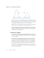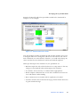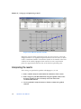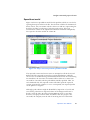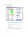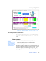
1
OptQuest® 2.3
User Manual
OptQuest developed by:
OptTek Logo
This manual, and the software described in it, are furnished under license and may
only be used or copied in accordance with the terms of the license agreement.
Information in this document is provided for informational purposes only, is subject to
change without notice, and does not represent a commitment as to merchantability or
fitness for a particular purpose by Decisioneering, Inc.
No part of this manual may be reproduced or transmitted in any form or by any means,
electronic or mechanical, including photocopying and recording, for any purpose
without the express written permission of Decisioneering, Inc.
Written, designed, and published in the United States of America.
To purchase additional copies of this document, contact the Technical Services or Sales
Department at the address below:
Decisioneering, Inc.
1515 Arapahoe St., Suite 1311
Denver, Colorado, USA 80202
Phone: +1 303-534-1515
Toll-free sales: 1-800-289-2550
Fax: 1-303-534-4818
© 1988-2006, Decisioneering, Inc.
Decisioneering® is a registered trademark of Decisioneering, Inc.
Crystal Ball® is a registered trademark of Decisioneering, Inc.
CB Predictor™ is a trademark of Decisioneering, Inc.
OptQuest® is a registered trademark of Optimization Technologies, Inc.
Microsoft® is a registered trademark of Microsoft Corporation in the U.S. and other
countries.
FLEXlm™ is a trademark of Macrovision Corporation.
Chart FX® is a registered trademark of Software FX, Inc.
is a registered trademark of Frontline Systems, Inc.
Other product names mentioned herein may be trademarks and/or registered
trademarks of the respective holders.
MAN-OQUM 020300-3 6/14/06
Contents
Welcome to OptQuest®
Who should use this program ................................................................... 1
How this manual is organized .................................................................. 2
Additional resources........................................................................................ 3
Technical support ..................................................................................... 3
Training .................................................................................................... 3
Consulting ................................................................................................. 3
Conventions used in this manual .................................................................... 4
Screen capture notes .......................................................................... 4
Chapter 1: Getting Started
What OptQuest does ....................................................................................... 6
Futura Apartments model ............................................................................... 7
Running OptQuest ................................................................................... 9
Closing the tutorial ................................................................................. 11
How OptQuest works .................................................................................... 11
Portfolio Allocation model ........................................................................... 13
Problem description ............................................................................... 13
Using OptQuest ...................................................................................... 14
Creating the Crystal Ball model ....................................................... 14
Defining decision variables .............................................................. 15
Selecting decision variables to optimize .......................................... 16
Specifying constraints ....................................................................... 18
Selecting the forecast objective ........................................................ 19
Running the optimization ................................................................ 20
Interpreting the results .................................................................... 22
Editing the optimization file ............................................................ 23
Interpreting results .......................................................................... 26
Portfolio allocation optimization summary ..................................... 26
Practice exercises .................................................................................... 27
Correlating assumptions .................................................................. 27
Changing the optimization objective ............................................... 27
Changing the number of trials ......................................................... 28
Using precision control .................................................................... 29
OptQuest and process capability................................................................... 30
Chapter 2: Understanding the Terminology
What is an optimization model?.................................................................... 32
Decision variables ................................................................................... 34
Constraints .............................................................................................. 35
Feasibility .......................................................................................... 35
Objective ................................................................................................. 36
Forecast statistics ..................................................................................... 36
OptQuest User Manual
i
Contents4
Minimizing or maximizing .............................................................. 37
Requirements ......................................................................................... 38
Feasibility ......................................................................................... 38
Requirement examples .................................................................... 38
Variable requirements ............................................................................ 39
Variable requirement example ........................................................ 39
Types of optimization models ...................................................................... 40
Discrete, continuous, or mixed? ............................................................ 40
Linear or nonlinear ................................................................................ 40
Deterministic or stochastic ..................................................................... 41
Examples of model types ....................................................................... 42
Statistics......................................................................................................... 43
Mean ....................................................................................................... 43
Median .................................................................................................... 44
Mode ....................................................................................................... 44
Standard deviation ................................................................................. 45
Variance ................................................................................................. 45
Percentile ................................................................................................ 46
Skewness ................................................................................................. 47
Kurtosis ................................................................................................... 47
Coefficient of variability ......................................................................... 48
Range (also range width) ........................................................................ 49
Mean standard error .............................................................................. 49
Certainty ................................................................................................. 49
Final value .............................................................................................. 50
Chapter 3: Setting Up and Optimizing a Model
Overview........................................................................................................ 52
Developing the Crystal Ball model ............................................................... 52
Developing the worksheet ...................................................................... 52
Defining assumptions, decision variables, and forecasts ....................... 54
Setting Crystal Ball run preferences ...................................................... 54
Selecting decision variables to optimize ....................................................... 55
Decision Variable Selection window ....................................................... 56
Specifying constraints .................................................................................. 58
Constraints window ................................................................................ 59
Selecting the forecast objective .................................................................... 60
Forecast Selection window ...................................................................... 62
Selecting options........................................................................................... 64
Options window ...................................................................................... 64
Time tab ........................................................................................... 65
Preferences tab ................................................................................. 66
Advanced tab .................................................................................... 67
ii
OptQuest User Manual
Contents
Running the optimization ............................................................................. 68
Start/Pause/Stop commands .................................................................... 69
Status And Solutions window .................................................................. 69
Status ................................................................................................ 69
Optimization File ............................................................................. 70
Solutions ........................................................................................... 70
Performance graph ................................................................................. 72
Bar graph ................................................................................................ 73
Optimization log ..................................................................................... 74
Efficient Frontier window ....................................................................... 75
Interpreting the results ................................................................................. 76
Running a solution analysis .................................................................... 77
Solution Analysis window ................................................................. 78
Running a longer simulation of the results ............................................ 80
Viewing charts in Crystal Ball .......................................................... 80
Chapter 4: Examples Using OptQuest
Overview ........................................................................................................ 82
Product mix ................................................................................................... 83
Problem statement .................................................................................. 83
Spreadsheet model ................................................................................. 84
OptQuest solution ................................................................................... 85
Practice exercise ...................................................................................... 86
Hotel design and pricing problem................................................................ 87
Problem statement .................................................................................. 87
Spreadsheet model ................................................................................. 88
OptQuest solution ................................................................................... 90
Budget-constrained project selection............................................................ 92
Problem statement .................................................................................. 92
Spreadsheet model ................................................................................. 93
OptQuest solution ................................................................................... 94
Practice exercise ...................................................................................... 95
Groundwater cleanup.................................................................................... 96
Problem statement .................................................................................. 96
Spreadsheet model ................................................................................. 97
OptQuest solution ................................................................................... 98
Practice exercise .................................................................................... 100
Oil field development ................................................................................. 101
Problem statement ................................................................................ 101
Spreadsheet model ............................................................................... 102
OptQuest solution ................................................................................. 103
Portfolio revisited ........................................................................................ 104
Problem statement ................................................................................ 104
OptQuest User Manual
iii
Contents4
Efficient portfolios ................................................................................ 105
Method 1: Efficient Frontier optimization ........................................... 107
Spreadsheet model ........................................................................ 107
OptQuest solution .......................................................................... 107
Method 2: Multiobjective optimization ............................................... 108
Spreadsheet model ........................................................................ 109
OptQuest solution .......................................................................... 111
Practice exercise ............................................................................. 112
Method 3: Arbitrage Pricing Theory ................................................... 112
Spreadsheet model ........................................................................ 114
OptQuest solution .......................................................................... 115
Tolerance analysis....................................................................................... 116
Problem statement ............................................................................... 116
Spreadsheet model ............................................................................... 118
OptQuest solution ................................................................................ 119
Maximizing assembly gap quality ........................................................ 121
Inventory system optimization.................................................................... 123
Problem statement ............................................................................... 123
Spreadsheet model ............................................................................... 125
OptQuest solution ................................................................................ 128
Practice exercise 1 ................................................................................ 131
Practice exercise 2 ................................................................................ 131
Drill bit replacement policy ........................................................................ 132
Problem statement ............................................................................... 132
Spreadsheet model ............................................................................... 133
OptQuest solution ................................................................................ 134
Practice exercise ................................................................................... 136
Chapter 5: Optimization Tips and Suggestions
Overview...................................................................................................... 138
Factors that affect search performance....................................................... 139
Simulation accuracy .............................................................................. 139
Number of simulation trials ........................................................... 140
Objective noisiness ......................................................................... 140
Number of decision variables ............................................................... 141
Initial values ......................................................................................... 141
Bounds and constraints ........................................................................ 142
Requirements ....................................................................................... 143
Variable requirements .......................................................................... 143
Complexity of the objective ................................................................. 144
Simulation speed .................................................................................. 144
Sensitivity analysis using a tornado chart ................................................... 145
iv
OptQuest User Manual
Contents
Appendix A: Advanced Optimization References
References ................................................................................................... 148
Appendix B: Menus and Keyboard Commands
OptQuest menus ......................................................................................... 150
Command key combinations and icons ...................................................... 151
OptQuest toolbar......................................................................................... 153
Bibliography ............................................................................................. 155
Glossary .................................................................................................... 159
Index ........................................................................................................... 169
OptQuest User Manual
v
Contents4
vi
OptQuest User Manual
1
Welcome to OptQuest®
Welcome to OptQuest® for Crystal Ball®!
OptQuest enhances Crystal Ball by automatically searching for and finding
optimal solutions to simulation models. Simulation models by themselves can
only give you a range of possible outcomes for any situation. They don't tell
you how to control the situation to achieve the best outcome
Using advanced optimization techniques, OptQuest finds the right
combination of variables that produces the best results possible. If you use
simulation models to answer questions such as “What are likely sales for next
month?”, now you can find the price points that maximize monthly sales. If
you asked, “What will production rates be for this new oil field?”, now you can
additionally determine the number of wells to drill to maximize net present
value. And if you wonder, “Which stock portfolio should I pick?” with
OptQuest, you can choose the one that yields the greatest profit with limited
risk.
Like Crystal Ball, OptQuest is easy to learn and easy to use. With its wizardbased design, you can start optimizing your own models in under an hour. All
you need to know is how to use a Crystal Ball spreadsheet model. From there,
this manual guides you step by step, explaining OptQuest terms, procedures,
and results.
Who should use this program
OptQuest is for the decision-maker, from the businessperson analyzing the
risk of new markets to the scientist evaluating experiments and hypotheses.
With OptQuest, you can make decisions that maximize the use of your
resources, time, and money.
OptQuest has been developed with a wide range of spreadsheet uses and
users in mind. You don’t need highly advanced statistical or computer
knowledge to use OptQuest to its full potential. All you need is a basic
working knowledge of your personal computer and the ability to use a Crystal
Ball spreadsheet model.
OptQuest User Manual
1
Introduction
How this manual is organized
The manual includes the following:
• Chapter 1 – “Getting Started”
This chapter contains two tutorials designed to give you a quick overview
of OptQuest’s features and to show you how to use the program. Read this
chapter if you need a basic understanding of OptQuest.
• Chapter 2 – “Understanding the Terminology”
This chapter contains a description of optimization models, their
components and types, and a review of basic statistics. Read this chapter
carefully if your modeling background is limited or if you need a review.
• Chapter 3 – “Setting Up and Optimizing a Model”
This chapter provides step-by-step instructions for setting up and
running an optimization in OptQuest.
• Chapter 4 – “Examples Using OptQuest”
This chapter contains nine optimization examples from a variety of fields
and disciplines.
• Chapter 5 – “Optimization Tips and Suggestions”
This chapter describes different factors that enhance the performance of
the program’s features.
• Appendices
•
A – “Advanced Optimization References”
A list of references describing OptQuest’s methodology, theory of
operation, and comparisons to other optimization software packages.
This appendix is designed for the advanced user.
•
B – “Menus and Keyboard Commands”
A summary of OptQuest’s menus and a list of the commands you can
execute directly from the keyboard.
• Bibliography
A list of related publications and textbooks.
• Glossary
A compilation of terms specific to OptQuest as well as statistical terms
used in this manual.
2
OptQuest User Manual
1
• Index
An alphabetical list of subjects and corresponding page numbers.
Additional resources
Decisioneering, Inc. offers these additional resources to increase the
effectiveness with which you can use our products.
Technical support
Technical Support is available for all registered customers with a current
maintenance agreement and a valid license authorization code. There are a
number of ways to reach Technical Support described in the README file in
the Crystal Ball installation folder. Online, see:
http://support.crystalball.com
Training
Decisioneering’s Training group offers a variety of courses throughout the
year to help improve how you make decisions. For more information about
Decisioneering courses, call one of these numbers Monday through Friday,
between 8:00 a.m. and 5:00 p.m. Mountain Time: 1-800-289-2550 (toll free in
US) or +1 303-534-1515, or visit the Decisioneering Web site:
http://www.crystalball.com/training
Consulting
Decisioneering's Services group provides consulting services including the full
range of risk analysis techniques from simulation, optimization, advanced
statistical analysis and exact probability calculations, to strategic thinking,
training, expert elicitation, and results communication to management. To
learn more about these consulting services, call 1-800-289-2550 Monday
through Friday, between 8:00 A.M. and 5:00 P.M. Mountain Time or see our
Web site at:
http://www.crystalball.com/consulting
OptQuest User Manual
3
Introduction
Conventions used in this manual
This manual uses the following conventions:
Text separated by > symbols means you select menu options in the sequence
shown, starting from the left. The following example means that you select
the Exit option from the File menu:
1. Select File > Exit.
Steps with attached icons mean you can click the icon instead of manually
selecting the menu options in the text. For example:
2. Select Define > Define Decision.
Notes provide additional information, expanding on the text. There are four
categories of notes:
OptQuest Note: Notes that provide additional directions or information about using
OptQuest.
Crystal Ball Note: Notes that provide additional directions or information about using
Crystal Ball.
Statistical Note: Notes that provide additional information about statistics.
Excel Note: Notes that provide additional information about using the program with
Microsoft Excel.
Screen capture notes
The screen captures in this document were taken in Excel 2000 on Windows
2000 and in Excel 2003 on Windows XP in Classic mode.
Due to round-off differences between various system configurations, you
might notice slightly different calculated results than those shown in the
examples.
4
OptQuest User Manual
Chapter 1
Getting Started
In this chapter
• What OptQuest does
• Portfolio Allocation model
• Futura Apartments model
• OptQuest and process capability
• How OptQuest works
This chapter has two tutorials that provide an overview of OptQuest’s features. The first
tutorial, the Futura Apartments model, is an extension of the model used in the Crystal
Ball documentation and finds the optimal rent for an apartment building. This model is
ready to run, so you can quickly see how OptQuest works.
The second tutorial, the Portfolio Allocation model, lets you set up and define an
optimization yourself. This model finds the optimal solution of investments that balances
the risk and the return of the portfolio.
The last section is note about using OptQuest to support Six Sigma and other quality
programs.
OptQuest User Manual
5
Chapter 1 | Getting Started
What OptQuest does
Glossary Term:
decision variable—
A variable in your model
that you can control.
In most simulation models, there are variables that you have control
over, such as how much to charge for rent or how much to invest.
These controlled variables are called decision variables. Finding the
optimal values for decision variables can make the difference between
reaching an important goal and missing that goal.
Obtaining optimal values generally requires that you search in an
iterative or ad hoc fashion. This involves running a simulation for an
initial set of values, analyzing the results, changing one or more
values, re-running the simulation, and repeating the process until you
find a satisfactory solution. This process can be very tedious and time
consuming even for small models, and it is often not clear how to
adjust the values from one simulation to the next.
Glossary Term:
optimal solution—
The set of decision
variable values that
achieves the best
outcome.
A more rigorous method systematically enumerates all possible
alternatives. Although this approach guarantees optimal solutions, it
has very limited application. Suppose that a simulation model
depends on only two decision variables. If each variable has 10
possible values, trying each combination requires 100 simulations
(102 alternatives). If each simulation is very short (e.g., 2 seconds),
then the entire process could be done in approximately 3 minutes of
computer time.
However, instead of two decision variables, consider six, then
consider that trying all combinations requires 1,000,000 simulations
(106 alternatives) or approximately 23 days of computer time. It is
easily possible for complete enumeration to take weeks, months, or
even years to carry out.
OptQuest overcomes the limitations of both the ad hoc and the
enumerative methods by intelligently searching for optimal solutions
to your simulation models. You describe your optimization problem
in OptQuest and then let it search for the values of decision variables
that maximize or minimize a predefined objective. In almost all cases,
OptQuest will efficiently find an optimal or near-optimal solution
among large sets of possible alternatives, even when exploring only a
small fraction of them.
6
OptQuest User Manual
1
Futura Apartments model
Futura Apartments model
The easiest way to understand what OptQuest does is to apply it to a simple
example. Suppose that you have recently purchased the Futura Apartments
complex. One of your critical decisions is the amount of rent to charge. You
have researched the situation and created a spreadsheet model to help you
make a knowledgeable decision.
From the analysis of the price structures and occupancy rates of similar
apartment complexes, you have estimated that demand for rental units is a
linear function of the rent charged, and is expressed as:
Number of units rented = -.1(rent per unit) + 85
for rents between $400 and $600.
In addition, you have estimated that operating costs will average about
$15,000 per month for the entire complex.
Crystal Ball Note: You can find the linear relationship of a dependent variable to one
or more independent variables using the regression tool in Microsoft Excel’s Analysis
Toolpak or CB Predictor.
To begin the tutorial:
1. Start Crystal Ball.
2. Open the Futura With OptQuest workbook from the Crystal Ball
Examples folder.
This spreadsheet is an enhanced version of the original Futura
Apartments example in Crystal Ball that contains no decision variables.
The Futura Apartments worksheet appears as shown in Figure 1.1.
OptQuest User Manual
7
Chapter 1 | Getting Started
Figure 1.1 Futura Apartments worksheet
In your spreadsheet, the rent is set to $500, where:
Number of units rented = -.1(500) + 85 = 35
and the total profit will be $2,500. If all the data were certain, the optimal
value for the rent could be found using a simple data table. However, in a
more realistic situation, monthly operating costs and the price-demand
function parameters (-.1 and 85) are not certain (probability distributions for
these assumptions are already defined for this example). Therefore,
determining the best rental price is not a straightforward exercise.
3. Before running OptQuest, select Run > Run Preferences and set the
following run preferences:
8
•
Maximum number of trials to run set to 500
•
Sampling method set to Latin hypercube
•
Sample Size For Latin Hypercube set to 500
•
Random Number Generation set to Use Same Sequence Of Random
Numbers with an Initial Seed Value of 999
OptQuest User Manual
1
Futura Apartments model
Running OptQuest
Use the following steps to run OptQuest for the Futura Apartments model.
1. To start OptQuest, select Run > OptQuest.
Crystal Ball Note: The Run > OptQuest command is not available if a simulation is
currently running or has not been reset. If you have trouble starting a new installation
of OptQuest, see the OptQuest Note on page 55.
The OptQuest welcome screen and window appear.
2. Select File > New.
The Decision Variable Selection window appears with the one decision
variable, Rent Per Unit. The check in the Select column indicates that the
variable is selected for optimization.
The lower bound on the variable is 400, the upper bound is 600, and the
suggested value is 500 (the current value in the worksheet). The variable
type is listed as Discrete (1).
3. Click OK in the Decision Variable Selection window.
The Constraints window appears. This problem has no constraints on the
decision variables, so do not add any here.
4. Click OK in the Constraints window.
Note: You need to click OK in each OptQuest window, even if you make no
changes, to assure that your OptQuest .opt file can be saved correctly.
The Forecast Selection window appears. In the model, the Profit Or Loss
cell is a forecast cell, and the objective is to maximize the mean (average)
profit.
5. Click the down arrow button under Select.
6. Select Maximize Objective for the Profit Or Loss forecast.
7. Click OK in the Forecast Selection window.
The Options window appears, letting you set various optimization
options.
8. Set the run time to 5 minutes.
The run time is on the Time tab.
OptQuest User Manual
9
Chapter 1 | Getting Started
9. Click OK in the Options window.
OptQuest prompts you to run the optimization.
10. Click Yes in the Run Optimization Now? dialog.
Glossary Term:
feasible solution—
A solution that satisfies any
constraints imposed on the
decision variables.
OptQuest begins to systematically search among the set of
feasible solutions for ones that improve the mean value of the
Profit Or Loss forecast.
As the optimization progresses, OptQuest collects the results of
the best solutions both in the Status And Solutions window and
on a performance graph.
Figure 1.2 OptQuest results for Futura Apartments model
For this optimization, the best rental price is $431 and will result in an
expected profit of $2,961.
OptQuest Note: When you limit the optimization by time, as in this example,
the number of simulations varies depending on your computer’s processing
speed. Thus, your results might not be exactly the same as those shown in Figure
1.2; however, they should be close. For more information on other factors that
affect the results, see “Factors that affect search performance” on page 139.
10
OptQuest User Manual
1
How OptQuest works
Closing the tutorial
To close the tutorial and return to Excel:
1. Select File > Exit.
OptQuest prompts you to save the optimization file before
closing.
2. Click No.
OptQuest asks whether to copy the selected values of the decision
variables into your spreadsheet. This lets you perform further
analyses using the selected solution.
3. Click Yes.
OptQuest restores the Crystal Ball simulation of the selected
solution to your spreadsheet. You can now analyze the forecast
windows, create reports, and use any other Crystal Ball options.
How OptQuest works
Traditional search methods (such as the one used in the Excel Solver)
work well when finding local solutions around a given starting point
with model data that are precisely known. These methods fail,
however, when searching for global solutions to real world problems
that contain significant amounts of uncertainty. Recent developments
in optimization have produced efficient search methods capable of
finding optimal solutions to complex problems involving elements of
uncertainty.
Glossary Term:
metaheuristics—
A family of optimization
approaches that
includes genetic
algorithms, simulated
annealing, tabu search,
scatter search, and their
hybrids.
OptQuest incorporates metaheuristics to guide its search algorithm
toward better solutions. This approach uses a form of adaptive
memory to remember which solutions worked well before and
recombines them into new, better solutions. Since this technique
doesn’t use the hill-climbing approach of ordinary solvers, it doesn't
get trapped in local solutions, and it doesn't get thrown off course by
noisy (uncertain) model data. You can find more information on
OptQuest’s search methodology in the references listed in Appendix
A.
Once you describe an optimization problem (by selecting decision
variables and the objective and possibly imposing constraints and
requirements), OptQuest invokes Crystal Ball to evaluate the
simulation model for different sets of decision variable values.
OptQuest evaluates the statistical outputs from the simulation model,
OptQuest User Manual
11
Chapter 1 | Getting Started
analyzes and integrates them with outputs from previous simulation runs, and
determines a new set of values to evaluate. This is an iterative process that
successively generates new sets of values. Not all of these values improve the
objective, but over time this process provides a highly efficient trajectory to
the best solutions.
The search process continues until OptQuest reaches some termination
criteria, either a limit on the amount of time devoted to the search or a
maximum number of simulations.
Determine a
new set of
values for
decision
variables
Crystal Ball Simulation
Generate
random
numbers for
assumption
cells
Calculate
entire
spreadsheet
Is
objective
better than
previous
ones?
Display
results in a
forecast chart
YES
Add new best
result to
Status And
Solutions
window
NO
Max
time or
number of
simulations
reached?
NO
Figure 1.3 OptQuest flow
12
OptQuest User Manual
YES
Stop and
prompt to
continue.
1
Portfolio Allocation model
Portfolio Allocation model
The remainder of this chapter contains a more detailed tutorial that will
guide you through setting up and running an optimization model using
Crystal Ball and OptQuest. If you are not familiar with basic optimization
terminology, such as “objectives” and “constraints,” review Chapter 2,
“Understanding the Terminology” on page 31.
Problem description
An investor has $100,000 to invest in four assets. Below is a list of the assets’
expected annual returns and the minimum and maximum amounts the
investor is comfortable allocating to each investment.
Investment
Annual return
Lower bound
Upper bound
Money market fund
3%
$0
$50,000
Income fund
5%
$10,000
$25,000
Growth and income fund
7%
$0
$80,000
Aggressive growth fund
11%
$10,000
$100,000
The source of uncertainty in this problem is the annual return of each asset.
The more conservative assets, the Income and Money Market funds, have
relatively stable annual returns, while the Aggressive Growth fund has higher
volatility.
The decision problem, then, is to determine how much to invest in each asset
to maximize the total expected annual return while maintaining the risk at an
acceptable level and keeping within the minimum and maximum limits for
each investment.
OptQuest User Manual
13
Chapter 1 | Getting Started
Using OptQuest
Using OptQuest involves the following steps:
1. Create a Crystal Ball model of the problem.
2. Define the decision variables within Crystal Ball.
3. In OptQuest, select decision variables to optimize.
4. Specify constraints on the decision variables.
5. Select the forecast objective and define any requirements.
6. Select optimization options.
7. Run the optimization.
8. Interpret the results.
Creating the Crystal Ball model
1. In Excel, open the Portfolio Allocation workbook from the Crystal Ball
Examples folder.
The worksheet for this problem is shown below.
Figure 1.4 Portfolio Allocation worksheet
14
OptQuest User Manual
1
Portfolio Allocation model
In this example, problem data are specified in rows 5 through 9. Model
inputs (the values of the decision variables), the model output (the
forecast objective), and the constraint (the total amount invested) are on
the bottom half of the worksheet.
This model already has the assumptions and forecast cells defined in
Crystal Ball.
2. Make sure the assumptions are defined as:
Assumption
Cell
Distribution
Parameters
Money market fund
C5
uniform
minimum: 2%
maximum: 4%
Income fund
C6
normal
mean: 5%
standard deviation: 5%
Growth and income
fund
C7
normal
mean: 7%
standard deviation: 12%
Aggressive growth fund
C8
normal
mean: 11%
standard deviation: 18%
Crystal Ball Note: If you need help viewing or defining assumptions or forecasts, see
your Crystal Ball User Manual.
3. Select Run > Run Preferences and set the following run preferences:
•
Maximum number of trials to run set to 500
•
Sampling method set to Latin hypercube
•
Sample Size For Latin Hypercube set to 500
•
Random Number Generation set to Use Same Sequence Of Random
Numbers with an Initial Seed Value of 999
Defining decision variables
The next step is to identify the decision variables in the model. This step is
not required when you create Crystal Ball simulation models. However, it is
mandatory when using OptQuest.
OptQuest User Manual
15
Chapter 1 | Getting Started
1. Define the first decision variable.
a.
Select cell C13.
b. Select Define > Define Decision.
c.
Set the Variable Type to Continuous.
d. Set the lower and upper bounds according to the problem
data (columns D and E in the worksheet), as shown in Figure
1.5.
Notice that you can enter cell references for cells D5 and E5.
After you complete an entry, the cell reference changes to its
value, as shown below.
Figure 1.5 Define Decision Variable window
Note: Previously, cell references were stored as relative values in
OptQuest. Now, they are stored as absolute values in OptQuest. This has
no effect on your model if you copy OptQuest values back to Excel. .Opt
files created in previous versions of OptQuest can be used with this version.
However, .opt files created or saved in OptQuest 2.3 cannot be used with
earlier versions.
2. Define the decision variables for cells C14, C15, and C16
according to the values in columns D and E of the worksheet, by
following the process described in step 1.
Selecting decision variables to optimize
1. Start OptQuest by selecting Run > OptQuest
Crystal Ball Note: If you have trouble starting a new installation of
OptQuest, see the OptQuest Note on page 55.
2. In OptQuest, select File > New or click New in the OptQuest
dialog.
16
OptQuest User Manual
1
Glossary Term:
wizard—
A feature that leads you
through the steps to create
an optimization model. This
wizard presents windows for
you to complete in the
proper order.
Portfolio Allocation model
A wizard starts, leading you through steps to create a new
optimization file. The wizard Welcome page outlines the steps
you will follow to create the optimization file. When you click OK,
the Decision Variable Selection window appears as shown in
Figure 1.6.
OptQuest Note: If you make a mistake at any point and want to start over
again:
a. Click Cancel.
b. Select Tools > Wizard.
Figure 1.6 OptQuest Decision Variable Selection window
Every decision variable defined in the Crystal Ball model appears
in the Decision Variable Selection window. The first column
indicates whether the variable has been selected for optimization.
The other columns show the bounds, suggested initial value, and
type for each variable.
3. Check the checkboxes by each decision variable to optimize all
decision variables.
4. Click OK.
The Constraints window appears (Figure 1.7). At first, the
formula area is blank.
OptQuest User Manual
17
Chapter 1 | Getting Started
Figure 1.7 OptQuest Constraints window
Specifying constraints
Glossary Term:
constraint—
A limitation that
restricts the possible
solutions to a model.
You must define
constraints in terms of
decision variables.
The Constraints window lets you specify any restrictions you can
define with the decision variables. The constraint in this model limits
the initial investment to $100,000.
The right side of the Constraints window lists the selected decision
variables. Constraints can use only linear combinations of these
variables. Enter constraining equations in the window, placing each
constraint on its own line.
OptQuest Note: To move a decision variable name to where the cursor is,
click a decision variable name in the Variables column. Use an asterisk to
multiply a constant and a variable (e.g., 3*X).
1. Click Sum All Variables.
2. Put a less-than sign (<) before the equals sign.
3. Enter the total investment as $100,000, so that the final
constraint looks like:
Money market fund + Income fund + Growth and income fund
+ Aggressive growth fund <= 100000
OptQuest Note: Don’t use “$” or a comma in the constraint. See “Constraints
window” on page 59 for other rules on constraints.
4. Click OK.
The Forecast Selection window appears as shown in Figure 1.8.
18
OptQuest User Manual
1
Glossary Term:
objective—
A formula in terms of
decision variables that
gives a mathematical
representation of the
model’s goal.
Glossary Term:
requirement—
A restriction on a
forecast statistic that
requires the statistic to
fall between specified
lower and upper limits
for a solution to be
considered feasible.
Portfolio Allocation model
Figure 1.8 OptQuest Forecast Selection window
Selecting the forecast objective
OptQuest requires that you select one forecast statistic to be the
objective to minimize or maximize. In addition to defining an
objective, you can define optimization requirements (described in
“Editing the optimization file” on page 23).
To select a forecast statistic to be the objective:
1. From the Select drop-down menu, select Maximize Objective.
The default statistic is the mean.
2. Click OK.
The Options window appears.
The goal for this example is to maximize the mean of the only
forecast cell, as shown in Figure 1.8. For many problems, the mean
(expected value) of the forecast is the most appropriate statistic to
optimize, but it need not always be.
For example, if an investor wants to maximize the upside potential of
his portfolio, he might want to use the 90th or 95th percentile as the
objective. The results would be solutions that have the highest
likelihood of achieving the largest possible returns. Similarly, to
minimize the downside potential of the portfolio, he might use the
5th or 10th percentile as the objective to minimize the possibility of
large losses.
You can use other statistics to realize different objectives. See
“Statistics” on page 43 for a description of all available statistics.
OptQuest User Manual
19
Chapter 1 | Getting Started
Running the optimization
In the Options window, you set options for controlling the optimization
process. The Options window has the following three tabs:
• Time
• Preferences
• Advanced
Figure 1.9 OptQuest Options window
Time tab
The Time tab lets you specify the total time that the system searches for the
best solutions for the decision variables. You can enter the number of minutes
to run an optimization, the number of simulations, or a date and time for the
process to stop. You can also select Automatic Stop to halt processing after the
indicated number of nonimproving solutions. The default optimization time
is 10 minutes.
Preferences and Advanced tabs
The Preferences and Advanced tabs contain additional options for controlling
the optimization process. See “Options window” on page 64 for descriptions
of these options.
1. For most processors, set the time limit to 10 minutes.
If you select a very long time limit, you can always terminate the search by
selecting Run > Stop or pressing Esc. Additionally, OptQuest prompts
you to extend the search when the time limit ends.
2. Click OK.
OptQuest prompts you to run the optimization.
20
OptQuest User Manual
1
Portfolio Allocation model
3. Click Yes.
The Status And Solutions window appears. Each time OptQuest identifies
a better solution during the optimization, it adds a new line to the Status
And Solutions window, showing the new objective value and the values of
the decision variables.
The time remaining and the simulation number under evaluation appear
in the upper left corner of the window. This information disappears when
the time limit is reached.
While the optimization is running, you can select these commands from
the View menu:
Performance
Graph
Shows a plot of the objective value as a function of the
number of simulations evaluated.
When using the wizard, this window opens automatically.
Bar Graph
Shows how the value of each decision variable changes
during the optimization search procedure.
Optimization
Log
Provides details of the sequence of solutions generated
during the search.
Efficient
Frontier
Plots a set of objective values found over the range of a
variable requirement (only available if there is a variable
requirement).
Figure 1.10 shows the Status And Solutions window after the optimization;
your results should be similar, but will depend on the speed of your processor
and other factors.
Figure 1.10 OptQuest solution results
The last line in the Status And Solutions window shows the best solution
found by OptQuest. All the money is allocated to the fund that has the
OptQuest User Manual
21
Chapter 1 | Getting Started
highest return, the Aggressive Growth fund, with the exception of the
minimal amount in the Income fund that the investor required.
The investor’s strategy maximized the return of the portfolio, but at a price:
high risk due to high volatility and little diversification. Is this really what the
investor wanted? To find out, the investor must interpret the results.
Interpreting the results
To interpret the OptQuest results:
1. After OptQuest completes the optimization, copy the optimization
results to your model by selecting Edit > Copy To Excel.
2. In Crystal Ball, view the forecast chart for the best simulation.
If it isn’t already onscreen, choose Analyze > Forecast Charts and select it
from the restored results files with names similar to optcbsav*.cbr.
Figure 1.11 Portfolio allocation forecast chart
Note: Forecast charts created by copying OptQuest data into Excel are only
available until OptQuest is closed. To clear them, choose Analyze > Close All in
Crystal Ball. If some remain, close OptQuest.
3. In the Forecast window, select View > Statistics.
The forecast statistics appear as shown in Figure 1.12.
22
OptQuest User Manual
1
Portfolio Allocation model
Figure 1.12 Portfolio allocation results statistics
Note that the standard deviation of the forecast is quite high, $16,342,
compared to the mean return of $10,374. The ratio of these two values, the
coefficient of variability, is shown as 1.58, or above 150%. Most of the money
allocated was in the Aggressive Growth fund, and the uncertainty of returns
for that fund was quite high, indicating the relative riskiness of the
investment.
Editing the optimization file
In portfolio management, controlling the variability of the solution to
minimize risk can be just as important as achieving large expected returns.
Suppose that this same investor wants to reduce the uncertainty of returns for
the portfolio, while still attempting to maximize the expected return. You
might want to find the best solution for which the standard deviation is much
lower, say, below $8,000.
Edit the optimization file to add this risk limitation and still maximize the
total expected return.
To edit the optimization file:
1. Return to OptQuest by clicking on the OptQuest button on the
Windows taskbar.
2. Open the Forecast Selection window. Use the button or select Tools >
Forecasts.
The window appears with the Total Expected Return forecast listed in the
first row.
OptQuest User Manual
23
Chapter 1 | Getting Started
3. Click in the existing forecast row.
4. Select Edit > Duplicate.
This creates a new row, with the forecast named Total Expected Return:2.
5. In the new row, select Requirement from the Select drop-down list.
6. From the Forecast Statistic drop-down list, select Std_Dev.
7. Set the upper bound to 8000.
This adds a requirement that the standard deviation of the expected
returns must be less than $8,000 for a solution to be considered feasible.
Figure 1.13 Forecast selection window with new requirement
8. Click OK.
9. Run the optimization by choosing Run > Start.
Figure 1.14 Portfolio allocation optimization results with risk
Before analyzing these new results in Crystal Ball, save the settings file and
exit OptQuest.
10. After OptQuest completes the optimization, save the current
optimization settings by selecting File > Save.
The Save As dialog appears.
24
OptQuest User Manual
1
Portfolio Allocation model
11. Save the file and name it Portfolio Allocation.opt.
12. Click Save.
This saves only the optimization settings; you must save the Crystal Ball
model separately in Excel. Optimization files automatically have the
extension .OPT, and you can reopen them by selecting File > Open or
clicking on Open the next time you run OptQuest.
Note: You need to click OK in each OptQuest window, even if you make no
changes, to assure that your OptQuest definition can be saved correctly.
13. To exit OptQuest, select File > Exit.
If you hadn't saved the optimization file yet, OptQuest would prompt you
to save it.
OptQuest asks if you want to copy the best solution into your spreadsheet
model.
14. Click Yes.
OptQuest copies the best solution into your Crystal Ball model and then
closes. You can also copy one of the other solutions into your Crystal Ball
model by selecting the corresponding row in the Status And Solutions
window before exiting. The associated simulation for the selected solution
is automatically restored when you exit, as shown below.
Figure 1.15 Best optimization solution
OptQuest User Manual
25
Chapter 1 | Getting Started
Interpreting results
This solution has significantly reduced the variability of the total expected
return, even though it now has a lower mean return. The portfolio achieved
this by finding the best diversification of conservative and aggressive
investments. Thus, the investor must face the trade-off between higher
returns with higher risk, and lower returns with lower risk.
How does this solution compare with the high-risk solution? Figure 1.16
shows the Crystal Ball results for the first solution beside results for the new
solution.
Higher-risk solution
Lower-risk solution
Figure 1.16 Simulation results comparison
Portfolio allocation optimization summary
The best OptQuest solution identified might not be the true optimal solution
to the problem, but should be close to the true optimal solution. The accuracy
of the results depends on the time limit you select for searching, the number
of trials per simulation, the number of decision variables, and the complexity
of the problem. With more decision variables, you need a larger number of
simulations. Further details of the search procedure can be found in Chapter
Chapter 5, “Optimization Tips and Suggestions” on page 137, and Appendix
A, “Advanced Optimization References”.
After solving an optimization problem with OptQuest, run a longer Crystal
Ball simulation using the optimal values of the decision variables to more
accurately compute the risks of the recommended solution.
26
OptQuest User Manual
1
Portfolio Allocation model
Practice exercises
Correlating assumptions
Very often, stocks, and therefore mutual funds, are positively correlated with
each other to some degree. This magnifies the variance of the stock portfolios
and their risk, and you must take this into account when evaluating portfolios.
Test how correlation affects the results of the optimization:
1. In Crystal Ball, define correlations of:
Money market fund
Money
market fund
Income fund
Growth and
income fund
Aggressive
growth fund
1.0
0.2
0.1
0.1
1.0
0.3
0.2
1.0
0.5
Income fund
Growth and income
fund
Aggressive growth
fund
1.0
To simplify setting up the matrix of correlations, use the Correlation
Matrix tool in Crystal Ball. For information on using this tool, see the
Crystal Ball User Manual.
2. Rerun the optimization.
3. Compare the results with the optimization results with no defined
correlation.
Changing the optimization objective
The objective in the Portfolio Allocation example was to maximize returns
subject to the requirement that the standard deviation remain under $8,000.
An equally valid objective is to minimize the standard deviation subject to the
requirement that the return be above a certain amount.
Change the optimization to make the objective minimizing the standard
deviation and the requirement that the mean be above some amount, such as
$8,000. How different are the optimization results?
The Portfolio Revisited example in Chapter 4 shows further how these two
objectives are related and discusses other types of objectives that incorporate
different risk factors.
OptQuest User Manual
27
Chapter 1 | Getting Started
Changing the number of trials
Increasing the number of trials used in the Crystal Ball simulations affects the
performance of OptQuest in two ways. First, in the same amount of time,
fewer simulations can be evaluated, decreasing the chances of converging to
an optimal or near-optimal solution. However, an increased number of trials
provides more discrimination among solutions since the accuracy of the
forecast statistics will be better.
To see the effects of increasing the number of trials:
1. Reopen the Portfolio Allocation.xls workbook and enter the original
decision variables and cell values.
2. In Crystal Ball, select Run > Run Preferences and change the
maximum number of trials from 500 to 2500.
3. Start OptQuest and reload the optimization settings file you saved
earlier.
4. Run another optimization.
Figure 1.17 shows the results of the optimization for the portfolio example
using the same amount of time, but 2500 trials per simulation instead of the
original value of 500. Note that fewer solutions were identified. Therefore,
you must make a trade-off between the accuracy of the results and the breadth
of the search. Experiment with differing numbers of trials and time limits to
see the differences in your results.
Figure 1.17 Results using 2500 trials per simulation
28
OptQuest User Manual
1
Portfolio Allocation model
Using precision control
You can use Crystal Ball’s precision control feature for several purposes:
• When you are unsure of how to set the number of trials used for Crystal
Ball simulations
• If you believe that the stability of the forecast statistics varies greatly
depending on the decision variable values
Precision control periodically calculates the accuracy of the forecast mean,
standard deviation, and any indicated percentile during the simulation. When
the simulation reaches a desired accuracy, it stops, regardless of the number of
trials already run.
This feature is especially useful for optimization models such as Portfolio
Allocation, where the forecast statistics are highly sensitive to the decision
variables. When OptQuest selects conservative investments, the variability of
the expected return is low and the statistics are relatively stable. When
OptQuest selects aggressive investments, the variability is high and the
statistics are relatively less stable. Using precision control increases your
forecast statistic accuracy while avoiding running too many trials when a
simulation reaches this accuracy quickly.
Note that finding the appropriate precision control settings might require
some trial and error. It can be challenging to decide whether to use absolute
or relative precision, what is the best precision value in either case, and which
statistics should receive precision control. For more information on setting the
precision control feature, see the Crystal Ball User Manual.
To see the effects of using precision control with the Portfolio Allocation
model:
1. In Crystal Ball, select Run > Run Preferences and change the
maximum number of trials from 500 to 2500.
This maximum limit is always in effect, even when precision control is
turned on. Therefore, when using precision control, you must increase
the maximum number of trials to let precision control achieve the
appropriate accuracy.
OptQuest User Manual
29
Chapter 1 | Getting Started
2. Turn on Precision Control.
a.
Select cell C17.
b. Select Define > Define Forecast.
c.
Click the More button in the Define Forecast dialog, then click the
Precision tab.
d. Check the Specify The Desired Precision For Forecast Statistics
option.
e.
Check the Mean checkbox.
f.
Use an absolute precision of 1000 units.
3. Start OptQuest and reload the optimization settings file you saved
earlier.
4. Run another optimization.
Experiment with various other precision control settings to see the difference
in the results.
OptQuest and process capability
You can use OptQuest to support process capability programs such as Six
Sigma, Design for Six Sigma (DFSS), Lean principles, and similar quality
initiatives. To do this, activate the Crystal Ball process capability features by
checking Calculate Capability Metrics on the Statistics tab of the Run
Preferences dialog. Once you do that, define a lower specification limit (LSL),
upper specification limit (USL), or both for a forecast in the Define Forecast
dialog. (You can also define an optional value target.) Once you have defined
at least one of the specification limits, you can view capability metrics for that
forecast. See the Crystal Ball Process Capability Guide for details.
If capability metrics are available for a forecast, you can optimize those
metrics in the Forecast Selection window of the OptQuest wizard. See
“Tolerance analysis” beginning on page 116 for an example. When you copy
the values back to the model, the optimized values, relevant forecast charts,
and the capability metrics table appear with the workbook as shown in Figure
4.30 on page 122.
Crystal Ball Note: The process capability metrics appear with other forecast statistics
in the Forecast Selection list. For a definition of each statistic, open OptQuest help and
look for “process capability metrics” on the Index tab. A list also appears in the Crystal
Ball Process Capability Guide.
30
OptQuest User Manual
Chapter 2
Understanding the Terminology
In this chapter
• What is an optimization model?
• Types of optimization models
• Statistics
The first part of this chapter describes the three major elements of an optimization model:
decision variables, constraints, and the objective. It also describes other elements, such as
requirements and forecast statistics, required for models with uncertainty.
The second part describes the different types of optimization models and how OptQuest
deals with the different types. It also presents examples of the different model types.
The last part describes the different statistics available to describe the objective.
OptQuest User Manual
31
Chapter 2 | Understanding the Terminology
What is an optimization model?
Glossary Term:
model—
A representation of a
problem or system in
a worksheet
application such as
Excel.
Glossary Term:
optimization model—
A model that seeks
to maximize or
minimize some
quantity, such as
profit or risk.
32
In today's competitive global economy, people are faced with many
difficult decisions. These decisions include allocating financial
resources, building or expanding facilities, managing inventories,
and determining product mix strategies. Such decisions might
involve thousands or millions of potential alternatives. Considering
and evaluating each of them would be impractical or even impossible.
A model can provide valuable assistance in analyzing decisions and
finding good solutions. Models capture the most important features
of a problem and present them in a form that is easy to interpret.
Models often provide insights that intuition alone cannot.
An optimization model has three major elements: decision variables,
constraints, and an objective.
decision
variables
Are quantities over which you have control; for
example, the amount of product to make, the number
of dollars to allocate among different investments, or
which projects to select from among a limited set.
constraints
Describe relationships among decision variables that
restrict the values of the decision variables. For
example, a constraint might ensure that the total
amount of money allocated among various investments
cannot exceed a specified amount, or at most one
project from a certain group can be selected.
objective
Gives a mathematical representation of the model's
objective, such as maximizing profit or minimizing cost,
in terms of the decision variables.
OptQuest User Manual
1
What is an optimization model?
Conceptually, an optimization model might look like Figure 2.1
Constant
Constant
Objective
Decision Variable
Decision Variable
Decision Variable
ts
in
tra
ns ter
Co Fil
Model
Deterministic Optimization Model
Figure 2.1 Schematic of an optimization model without uncertainty
The solution to an optimization model provides a set of values for the
decision variables that optimizes (maximizes or minimizes) the associated
objective. If the world were simple and the future were predictable, all data in
an optimization model would be constant, making the model deterministic.
In many cases, however, a deterministic optimization model can’t capture all
the relevant intricacies of a practical decision environment. When model data
are uncertain and can only be described probabilistically, the objective will
have some probability distribution for any chosen set of decision variables.
You can find this probability distribution by simulating the model using
Crystal Ball.
An optimization model with uncertainty has several additional elements:
assumptions
Capture the uncertainty of model data using probability
distributions.
forecasts
Are frequency distributions of possible results for the model.
forecast
statistics
Are summary values of a forecast distribution, such as the mean,
standard deviation, or variance. You control the optimization by
maximizing, minimizing, or restricting forecast statistics.
requirements
Are additional restrictions on forecast statistics. You can set upper
and lower limits for any statistic of a forecast distribution. You can
also define a range of requirement values by defining a variable
requirement.
OptQuest User Manual
33
Chapter 2 | Understanding the Terminology
Assumptions
Assumptions
Objective
(Forecast)
Decision Variable
Decision Variable
Model
t
en
m
ire r
qu lte
R e Fi
ts
in
tra
ns lter
C o Fi
Decision Variable
s
Optimization Model With Uncertainty
Figure 2.2 Schematic of an optimization model with uncertainty
Decision variables
Decision variables are variables in your model that you can control, such as
how much rent to charge or how much money to invest in a mutual fund.
Decision variables aren’t required for Crystal Ball models, but are required for
OptQuest models. You define decision variables in Crystal Ball using Define
> Define Decision.
When you define a decision variable in Crystal Ball, you define its:
bounds
Defines the upper and lower limits for the variable. OptQuest
searches for solutions for the decision variable only within these
limits.
type
Defines whether the variable is discrete or continuous. A discrete
variable can assume integer or non-integer values and must have
a defined step size that is greater than 0 (integer or non-integer).
A continuous variable requires no step size, and any given range
contains an infinite number of possible values.
step size
Defines the difference between successive values of a discrete
decision variable in the defined range. For example, a discrete
decision variable with a range of 1 to 5 and a step size of 1 can
only take on the values 1, 2, 3, 4, or 5; a discrete decision variable
with a range of 0 to 2 with a step size of 0.25 can only take on the
values 0, 0.25, 0.5, 0.75, 1.0, 1.25, 1.5, 1.75, and 2.0.
In an optimization model, you select which decision variables to optimize
from a list of all the defined decision variables. The values of the decision
34
OptQuest User Manual
1
What is an optimization model?
variables you select will change with each simulation until the best value for
each decision variable is found within the available time limit.
Constraints
Constraints restrict the decision variables by defining relationships among
them. For example, if the total amount of money invested in two mutual funds
must be $50,000, you can define this as:
mutual fund #1 + mutual fund #2 = 50000
OptQuest only considers combinations of values for the two mutual funds
whose sum is $50,000.
Or if your budget restricts your spending on gasoline and fleet service to
$2,500, you can define this as:
gasoline + service <= 2500
In this case, OptQuest considers only combinations of values for gasoline and
service at or below $2,500.
OptQuest Note: Not all optimization models need constraints.
Feasibility
A feasible solution is one that satisfies all constraints. Infeasibility occurs when
no combination of values of the decision variables can satisfy a set of
constraints. Note that a solution (i.e., a single set of values for the decision
variables) can be infeasible, by failing to satisfy the problem constraints, and
this doesn’t imply that the problem or model itself is infeasible.
For example, suppose that in the Portfolio Allocation problem the investor
insists on finding an optimal investment portfolio with the following
constraints:
Income fund + Aggressive growth fund <= 10000
Income fund + Aggressive growth fund >= 12000
Clearly, there is no combination of investments that will make the sum of the
income fund and aggressive growth fund no more than $10,000 and at the
same time greater than or equal to $12,000.
OptQuest User Manual
35
Chapter 2 | Understanding the Terminology
Or, for this same example, suppose the bounds for a decision variable were:
$15,000 <= Income fund <= $25,000
And a constraint was:
Income fund <= 5000
This also results in an infeasible problem.
You can make infeasible problems feasible by fixing the inconsistencies of the
relationships modeled by the constraints. OptQuest detects optimization
models that are constraint-infeasible and reports them to you.
If a model is constraint-feasible, OptQuest will always find a feasible solution
and search for the optimal solution (i.e., the best solution that satisfies all
constraints).
Objective
Each optimization model has one objective, a forecast cell, that
mathematically represents the model’s objective in terms of the assumption
and decision cells. OptQuest’s job is to find the optimal value of the objective
by selecting and improving different values for the decision variables.
When model data are uncertain and can only be described using probability
distributions, the objective itself will have some probability distribution for
any set of decision variables. You can find this probability distribution by
defining the objective as a forecast and using Crystal Ball to simulate the
model.
Forecast statistics
You can’t use an entire forecast distribution as the objective, but must
characterize the distribution using a single summary measure for comparing
and choosing one distribution over another. Thus, to use OptQuest, you must
select a statistic of one forecast to be the objective. You must also select
whether to maximize or minimize the objective.
36
OptQuest User Manual
1
What is an optimization model?
Figure 2.3 Forecast shown with mean statistic
The statistic you choose depends on your goals for the objective. For
maximizing or minimizing some quantity, the mean or median are often used
as measures of central tendency, with the mean being the more common of
the two. For highly skewed distributions, however, the mean might become
the less stable (having a higher standard error) of the two, and so the median
becomes a better measure of central tendency.
For minimizing overall risk, the standard deviation or the variance of the
objective are the two best statistics to use. For maximizing or minimizing the
extreme values of the objective, a low or high percentile might be the
appropriate statistic. For controlling the shape or range of the objective, the
skewness, kurtosis, or certainty statistics might be used. For more information
on these statistics, see “Statistics” on page 43.
Minimizing or maximizing
Whether you want to maximize or minimize the objective depends on which
statistic you select to optimize. For example, if your forecast is profit and you
select the mean as the statistic, you would want to maximize the profit mean.
However, if you select the standard deviation as the statistic, you might want
to minimize it to limit the uncertainty of the forecast.
OptQuest User Manual
37
Chapter 2 | Understanding the Terminology
Requirements
Requirements restrict forecast statistics. These differ from constraints, since
constraints restrict decision variables (or relationships among decision
variables).
OptQuest Note: Requirements are sometimes called “probabilistic constraints,”
“chance constraints,” or “goals” in other literature.
When you define a requirement, you first select a forecast (either the objective
forecast or another forecast). As with the objective, you then select a statistic
for that forecast, but instead of maximizing or minimizing it, you give it an
upper bound, a lower bound, or both (a range).
Feasibility
Like constraints, requirements must be satisfied for a solution to be
considered feasible. When an optimization model includes requirements, a
solution that is constraint-feasible might be infeasible with respect to one or
more requirements.
After first satisfying constraint feasibility, OptQuest assumes that the user's
next highest priority is to find a solution that is requirement-feasible.
Therefore, it concentrates on finding a requirement-feasible solution and
then on improving this solution, driven by the objective in the model.
Requirement examples
In the Portfolio Allocation example of Chapter 1, the investor wants to impose
a condition that limits the standard deviation of the total return. Because the
standard deviation is a forecast statistic and not a decision variable, this
restriction is a requirement.
The following are some examples of requirements on forecast statistics that
you could specify:
95th percentile >= 1,000
-1 <= skewness <= 1
Range 1,000 to 2,000 >= 50% certainty
38
OptQuest User Manual
1
What is an optimization model?
Variable requirements
Variable requirements let you define a range for a requirement bound (instead
of a single point) and a number of points to check within the range. OptQuest
runs one full optimization for each point in the range, starting with the most
limiting requirement point. This lets you see the effects of tightening or
loosening a requirement.
When you define a variable requirement, you first select a forecast (either the
objective forecast or another forecast). Like the objective or the requirement,
you then select a statistic for that forecast, but instead of maximizing or
minimizing it, you select to restrict the upper bound or the lower bound. You
then define the upper or lower bound with a range.
Variable requirement example
In the Portfolio Allocation example of Chapter 1, the investor wants to impose
a condition that limits the standard deviation of the total return. Because the
standard deviation is a forecast statistic and not a decision variable, this
restriction is a requirement.
However, if the investor wants to see if a small increase in the requirement
could create a sharp increase in the investment return, the investor can set
this as a Variable Requirement Upper Bound (since this limits the maximum
standard deviation). The investor can define this upper bound with a lower
limit of 8000 and an upper limit of 10,000.
OptQuest User Manual
39
Chapter 2 | Understanding the Terminology
Types of optimization models
Discrete, continuous, or mixed?
Optimization models can be classified as:
Model
Have:
discrete
Only discrete decision variables.
continuous
Only continuous decision variables.
mixed
Both discrete and continuous decision variables.
For more information on discrete and continuous decision variables, see
“Decision variables” on page 34.
1
3
5
7
Discrete variable
Staff requirements
9
Continuous variable
Prime interest rate
Figure 2.4 Comparison of discrete and continuous decision variables
Linear or nonlinear
An optimization model can be linear or nonlinear, depending on the form of
the mathematical relationships used to model the objective and constraints.
In a linear relationship, all terms in the formulas only contain a single
variable multiplied by a constant. For example, 3x - 1.2y is a linear
relationship since both the first and second term only involve a constant
multiplied by a variable. Terms such as x2, xy, 1/x, or 3.1x make nonlinear
relationships. Any models that contain such terms in either the objective or a
constraint are classified as nonlinear.
OptQuest can handle linear or nonlinear objectives, but the Constraints
window can handle only linear constraints. For information on defining linear
or nonlinear constraints, see “Specifying constraints” on page 58.
40
OptQuest User Manual
1
Types of optimization models
Linear function
Number of personnel vs. employee costs
Nonlinear function
Population growth over time
Figure 2.5 Comparison of linear and nonlinear functions
Deterministic or stochastic
Glossary Term:
stochastic—
A model or system
with one or more
random variables.
Optimization models might also be classified as deterministic or
stochastic, depending on the nature of the model data. In a
deterministic model, all input data are constant or assumed to be
known with certainty. In a stochastic model, some of the model data
are uncertain and are described with probability distributions.
Stochastic models are much more difficult to optimize because they
require simulation to compute the objective. While OptQuest is
designed to solve stochastic models using Crystal Ball, it is also
capable of solving deterministic models. See “Selecting options” on
page 64.
Deterministic
Excel worksheet result
Stochastic
Crystal Ball simulation result
Figure 2.6 Comparison of deterministic and stochastic results
OptQuest User Manual
41
Chapter 2 | Understanding the Terminology
Examples of model types
To illustrate these model types, consider the Futura Apartments model used
in the first tutorial in Chapter 1. The decision variable (there is only one in
this case) is the rent per unit to charge. The objective is to maximize net
profit, which can be expressed as:
Net profit
= Revenue - Expenses
= (Number of units rented)(Rent/unit) - Monthly expenses
= (-0.1*Rent/unit + 85)*(Rent/unit) - Monthly expenses
There are no constraints in this example.
The Portfolio Allocation model in the second tutorial in Chapter 1 is more
complex. The decision variables are the amounts to allocate to a money
market fund, an income fund, a growth and income fund, and an aggressive
growth fund. The objective is to maximize the total expected annual return:
0.03*Money market fund + 0.05*Income fund + 0.07*Growth and
income fund + 0.11*Aggressive growth fund
There is one constraint, the total amount of money available to invest:
Money market fund + Income fund + Growth and income fund +
Aggressive growth fund <= 100000
If all returns for this example are constant rather than uncertain, then the
model is a continuous, linear, deterministic optimization model. All variables
are continuous; that is, they might assume any fractional value. The objective
is linear. Finally, the returns on each prospective investment are known with
certainty (i.e., the returns are “true” values, not distributions); thus, the model
is deterministic.
In contrast, the Futura Apartments model is discrete, nonlinear, and
stochastic. It is discrete because the decision variable is defined in whole
dollar increments. It is nonlinear because the objective (net profit) includes a
term that is the square of the decision variable (rent/unit). Finally, it is
stochastic because the price-demand function parameters and the monthly
expenses are not known with certainty.
OptQuest is designed to handle any and all types of optimization models with
only one limitation: constraints must be linear, unless you model the
nonlinear constraints as requirements. See “Specifying constraints” on
page 58.
42
OptQuest User Manual
1
Statistics
Statistics
This section explains the forecast statistics you can choose in OptQuest to
define the optimization’s objective. These terms are listed in the Statistics
window when you run a simulation in Crystal Ball and in the reports that you
can create.
Statistic
See:
Mean
page 43
Median
page 44
Mode
page 44
Standard deviation
page 45
Variance
page 45
Percentile
page 46
Skewness
page 47
Kurtosis
page 47
Coefficient of variability
page 48
Range (also range width)
page 49
Mean standard error
page 49
Certainty
page 49
Final value
page 50
The formulas for many of the statistics are listed in the Crystal Ball User
Manual.
Mean
The mean of a set of values is found by adding the values and dividing their
sum by the number of values. The term “average” usually refers to the mean.
For example, 5.2 is the mean or average of 1, 3, 6, 7, and 9.
OptQuest User Manual
43
Chapter 2 | Understanding the Terminology
Median
The median is the middle value in a set of values. For example, 6 is the
median of 1, 3, 6, 7, and 9, while the mean is 5.2.
If there is an odd number of values, the median is found by placing the values
in order from smallest to largest and then selecting the middle value.
If there is an even number of values, the median is the mean of the two
middle values.
Mode
The mode is the value that occurs most frequently in a set of values. In
general, the greatest degree of clustering occurs at the mode.
The modal wage, for example, is the one received by the greatest number of
workers. The modal color for a new product is the one preferred by the
greatest number of consumers.
In a perfectly symmetrical distribution like the normal distribution (shown
below on the left), the mean, median, and mode converge at one point.
In an asymmetrical or skewed distribution like the lognormal distribution on
the right, the mean, median, and mode tend to spread out, as shown below.
Mode
Median
Mean
Mean
Median
Mode
Figure 2.7 Comparison of normal and skewed distributions
Crystal Ball Note: When using continuous distributions, it is likely that your forecast
will not have two values that are exactly the same. When this occurs, Crystal Ball sets
the mode to ‘---’ to indicate that the mode is undefined.
44
OptQuest User Manual
1
Statistics
Standard deviation
The standard deviation is the square root of the variance for a distribution of
values. Like the variance, it is a measure of dispersion about the mean.
For example, you can calculate the standard deviation of the values 1, 3, 6, 7,
and 9 by finding the square root of the variance that is calculated in the
variance example below.
The standard deviation, denoted as s , is calculated from the variance as
follows:
s =
10.2 = 3.19
See “ Variance” calculation below.
Variance
Variance is a measure of the dispersion, or spread, of a set of values about the
mean. When values are close to the mean, the variance is small. When values
are widely scattered about the mean, the variance is larger.
To calculate the variance of a set of values:
1. Find the mean or average.
2. For each value, calculate the difference between the value and the mean.
3. Square these differences and sum the squares.
4. Divide by n-1, where n is the number of differences.
For example, suppose your values are 1, 3, 6, 7, and 9. The mean is 5.2. The
2
variance, denoted by s , is calculated as follows:
2
2
2
2
2
2
( 1 – 5.2 ) + ( 3 – 5.2 ) + ( 6 – 5.2 ) + ( 7 – 5.2 ) + ( 9 – 5.2 )
s = ------------------------------------------------------------------------------------------------------------------------------------------------5–1
40.8
= ---------- = 10.2
4
OptQuest Note: The calculation uses n-1 instead of n to correct for the fact that sample
variances are slightly smaller than the variance of the entire population.
OptQuest User Manual
45
Chapter 2 | Understanding the Terminology
Percentile
A percentile is a number on a scale of zero to one hundred that indicates the
percent of a distribution that is equal to or below a value (default definition).
Standardized tests usually report results in percentiles. So if you were at the 95
percentile, that means you scored better than 95% of the people who took the
test. This doesn’t mean you answered 95% of the questions correctly. You
might have answered only 20% correctly, but that was better than 95% of the
people who took the test.
As another example, suppose you want to be 90% sure that you put enough
money away for your retirement. You might create a model with all the
uncertain variables, such as annual return on your investments, inflation, and
expenses at retirement. The resulting distribution shows the most likely
investment needed, but if you select the mean, you have a 50% chance of not
having enough money. So you choose the value at the 90 percentile, which
leaves only a 10% chance of not having enough money.
10%
20%
30% 50% 70%
40% 60%
80%
90%
Figure 2.8 Percentiles for a normal distribution
Crystal Ball Note: You can reverse the meaning of the percentiles by changing the
setting in the Run Preferences > Statistics dialog. For more information, see the Crystal
Ball User Manual.
46
OptQuest User Manual
1
Statistics
Skewness
A distribution of values (a frequency distribution) is said to be “skewed” if it is
not symmetrical.
For example, suppose the curves in the example below represent the
distribution of wages within a large company.
A
B
Figure 2.9 Comparison of positive and negative skewness
Curve A illustrates positive skewness (skewed “to the right”) where most of the
wages are near the minimum rate, although some are much higher. Curve B
illustrates negative skewness (skewed “to the left”) where most of the wages are
near the maximum, although some are much lower.
If you describe the curves statistically, curve A is positively skewed and might
have a skewness coefficient of 0.5, while curve B is negatively skewed and
might have a -0.5 skewness coefficient.
A skewness value greater than 1 or less than -1 indicates a highly skewed
distribution. A value between 0.5 and 1 or -1 and -0.5 indicates a moderately
skewed distribution. A value between -0.5 and 0.5 indicates a fairly
symmetrical distribution.
Kurtosis
Kurtosis refers to the peakedness of a distribution. For example, a perfectly
symmetrical distribution of values can look either very “peaked” or very “flat,”
as illustrated in Figure 2.10.
OptQuest User Manual
47
Chapter 2 | Understanding the Terminology
A
B
Figure 2.10 Comparison of peaked and flat kurtosis
Suppose the curves in the example above represent the distribution of wages
within a large company. Curve A is fairly peaked, since most of the employees
receive about the same wage with few receiving very high or low wages. Curve
B is flat topped, indicating that the wages cover a wider spread.
Describing the curves statistically, Curve A is fairly peaked, with a kurtosis of
about 4. Curve B, which is fairly flat, might have a kurtosis of 2.
A normal distribution is usually used as the standard of reference and has a
kurtosis of 3. Distributions with a kurtosis value less than 3 are described as
platykurtic (meaning flat) and distributions with a kurtosis value greater than
3 are leptokurtic (meaning peaked).
Coefficient of variability
The coefficient of variability measures the variability of a forecast compared to
the mean value. Since this statistic is independent of the forecast units, you
can use it to compare the variability of two or more forecasts, even when the
forecast scales differ.
For example, if you are comparing the forecast for a penny stock with the
forecast for a stock on the New York Stock Exchange, you would expect the
average variation (standard deviation) of the penny stock price to appear
smaller than the variation of the NYSE stock. However, if you compare the
coefficient of variability statistic for the two forecasts, you will likely observe
that the penny stock shows significantly more variation on a relative scale.
The coefficient of variability typically ranges from a value greater than 0 to 1.
It may exceed 1 in a small number of cases in which the standard deviation of
the forecast is unusually high.
48
OptQuest User Manual
1
Statistics
The coefficient of variability is calculated by dividing the standard deviation
by the mean, as follows:
s
coefficient of variability = -x-
To present this in percentage form, simply multiply the result of the above
calculation by 100.
Range (also range width)
The range minimum is the smallest number in a set, and the range maximum
is the largest number.
The range is the difference between the range minimum and the range
maximum. For example, if the range minimum is 10 and the range maximum
is 70, then the range is 60.
Mean standard error
The mean standard error statistic lets you estimate the accuracy of your
simulation results and thus determine how many trials are necessary to ensure
an acceptable level of error. This statistic tells you the probability of the
estimated mean deviating from the true mean by more than a specified
amount. The probability that the true mean of the forecast is within plus or
minus the mean standard error of the estimated mean is approximately 68%.
Statistical Note: The mean standard error statistic only provides information on the
accuracy of the mean and can be used as a general guide to the accuracy of the
simulation. The standard error for other statistics, such as mode and median, will
probably differ from the mean standard error.
Certainty
Certainty describes the percentage of simulation results that fall within a
range. For instance, in the portfolio allocation example from Chapter 1, if
your objective was to achieve the highest probability of a minimum return of
$8,000, you might choose a range of $8,000 to +Infinity and then maximize
the certainty of this range.
When you select the certainty of a forecast as a requirement, you must first
define the range that you want the forecast values to fall in, such as between
OptQuest User Manual
49
Chapter 2 | Understanding the Terminology
$8,000 and positive infinity. Then you must define in the Lower Bounds
column the minimum percentage of results that must fall in the defined range
for the solution to be feasible, such as 60%.
In Figure 2.11, the certainty range is $0 to $26.1 million and the certainty
level is 75%.
Certainty
Figure 2.11 Forecast certainty
By default, the range of certainty is from negative infinity to positive infinity.
The certainty for this range is always 100%.
Final value
The final value is the last value that is calculated for a forecast during a
simulation. The final value is useful when a forecast contains a function that
accumulates values across the trials of a simulation, or is a function that
calculates the statistic of another forecast. See “Oil field development” on
page 101 and “Tolerance analysis” on page 116 for examples using final
value.
50
OptQuest User Manual
Chapter 3
Setting Up and Optimizing a Model
In this chapter
• Overview
• Developing the Crystal Ball model
• Selecting decision variables to optimize
• Specifying constraints
• Selecting the forecast objective
• Selecting options
• Running the optimization
• Interpreting the results
This chapter describes how to use OptQuest, step by step. It also gives details about each of
the windows and dialogs in OptQuest, including all the fields and options.
OptQuest User Manual
51
Chapter 3 | Setting Up and Optimizing a Model
Overview
To set up and optimize a model with OptQuest, follow these steps:
1. Create a Crystal Ball model of the problem.
2. Define the decision variables within Crystal Ball.
3. In OptQuest, select decision variables to optimize.
4. Specify any constraints on the decision variables.
5. Select the forecast objective and define any requirements.
6. Select optimization options.
7. Run the optimization.
8. Interpret the results.
You perform steps 1 and 2 in Crystal Ball, 3 through 7 in OptQuest, and 8 in
both.
Developing the Crystal Ball model
Before using OptQuest, you must first develop a useful Crystal Ball model.
This entails building a well-tested spreadsheet in Excel, and then defining
assumptions and forecast cells using Crystal Ball. You should refine the
Crystal Ball model and run several simulations to ensure that the model is
working correctly and that the results are what you expect.
Developing the worksheet
You should build your spreadsheet model using principles of good design,
since this makes understanding and modifying it easier.
The spreadsheet should include:
• A descriptive title.
• An input data area separate from the output and any working space. Place
all input variables in their own cells where you can later define them as
assumptions or decision variables.
• A working space for all complex calculations, formulas, and data tables.
• A separate output section that provides the model results.
52
OptQuest User Manual
1
Developing the Crystal Ball model
Examine the Portfolio Allocation spreadsheet model below, introduced in
Chapter 1, for an example.
Figure 3.1 Portfolio Allocation model
Note that all input variables (assumptions and decision variables) are in rows
5 through 8 and rows 13 through 16, and forecast cells reference the cells in
their calculations, not values directly. Therefore, you could easily change any
values, and the forecast calculations would be automatically updated.
Other tips that improve the usefulness of your spreadsheet are:
• Reference input data only with cell references or range names so that any
changes are automatically reflected throughout the worksheet.
• Use formats, such as currency or comma formats, appropriately.
• Divide complex calculations into several cells to minimize the chance for
error and enhance understanding.
• Place comments next to formula cells for explanation, if needed.
• Consult a reference such as those listed on page 156 for further discussion
of good worksheet design.
OptQuest User Manual
53
Chapter 3 | Setting Up and Optimizing a Model
Defining assumptions, decision variables, and forecasts
Once you build and test the spreadsheet, you can define your assumptions,
decision variables, and forecasts. For more information on defining
assumptions, decision variables, and forecasts, see the Crystal Ball User Manual.
Setting Crystal Ball run preferences
To set Crystal Ball run preferences, select Run > Run Preferences. For
optimization purposes, you should usually use the following Crystal Ball
settings:
• Trials tab — Maximum number of trials to run set to 500.
Central-tendency statistics such as mean, median, and mode usually
stabilize sufficiently at 500 trials per simulation. Tail-end percentiles and
maximum and minimum range values generally require at least 1,000
trials.
• Sampling tab — Sampling method set to Latin hypercube.
Latin hypercube sampling increases the quality of the solutions, especially
the accuracy of the mean statistic.
• Sampling tab — Random Number Generation set to Use Same Sequence
Of Random Numbers with an Initial Seed Value of 999.
The initial seed value determines the first number in the sequence of
random numbers generated for the assumption cells. This lets you repeat
simulations using the same set of random numbers to accurately compare
the simulation results.
Crystal Ball Note: When your Crystal Ball forecast has extreme outliers, run the
optimization with several different seed values or a random seed.
• Trials tab — Check Precision Control Every 50 Trials
OptQuest checks ongoing simulations periodically to stop and eliminate
simulations that have a small chance of improving upon the best solution.
• Speed tab — Chart Windows > Redraw Every 1 Second(s)
54
OptQuest User Manual
1
Selecting decision variables to optimize
Selecting decision variables to optimize
After you define the assumptions, decision variables, and forecasts in Crystal
Ball, you can begin the optimization process in OptQuest. The first step of
this process is selecting decision variables to optimize. The values of these
decision variables will change with each simulation until OptQuest finds
values that yield the best objective. For some analyses, you might fix the values
of certain decision variables and optimize the rest.
1. Start OptQuest by choosing Run > OptQuest
OptQuest Note: If you are unable to start a new installation of OptQuest, try logging
in with administrator rights.
2. In OptQuest, select File > New.
A wizard starts, leading you through the windows to complete for the
optimization. The Decision Variable Selection window appears first,
listing every decision variable defined in all open Excel workbooks. For
details on the fields in this window, see “Decision Variable Selection
window” below.
3. Select which decision variables to optimize.
By default, all are selected.
4. Optionally, change the lower and upper bounds for each decision
variable.
By default, OptQuest uses the limits you entered when you defined the
decision variables. The tighter the bounds you specify, the fewer values
OptQuest must search to find the optimal solution. However, this
efficiency comes at the expense of missing the optimal solution if it lies
outside the specified bounds.
5. Optionally, change the start values for each decision variable in the
Suggested Value column.
By default, OptQuest uses the cell values in your Crystal Ball model. If the
suggested values lie outside of the specified bounds or do not meet the
problem constraints, OptQuest ignores them.
6. Check that the Type column indicates the correct type of values.
You can change the variable type here or in the Define Decision Variable
dialog of Crystal Ball.
7. Click OK.
The Constraints window appears next.
OptQuest User Manual
55
Chapter 3 | Setting Up and Optimizing a Model
Decision Variable Selection window
The Decision Variable Selection window lets you select which defined decision
variables to optimize. To access this window, either:
• Run the wizard.
• Select Tools > Decision Variables.
• Click the Decision Variables icon.
Figure 3.2 The Decision Variable Selection window
The columns and buttons in this window are:
Table 3.1 Decision Variable Selection window elements
Element
56
Action
Select
Indicates whether OptQuest will optimize the variable. A check
indicates that the decision variable will be optimized.
The default is to optimize all decision variables.
Variable Name
Displays the variable name defined in Crystal Ball. This field is
for display only.
Lower Bound
Is the lower limit for the variable. If you change this field,
OptQuest automatically updates the lower limit in Crystal Ball
with the new value.
The default is the variable’s lower bound defined in Crystal Ball.
Suggested
Value
Is the initial value OptQuest uses at the beginning of
optimization. For unselected decision variables, OptQuest
always uses the suggested value to evaluate the objective.
The default is the cell value in the worksheet. If the cell value is
outside the range between the upper and lower bounds, the
midpoint of the decision variable is used.
OptQuest User Manual
1
Selecting decision variables to optimize
Table 3.1 Decision Variable Selection window elements (Continued)
Element
Action
Upper Bound
Is the upper limit for the variable. If you change this field,
OptQuest automatically updates the upper limit in Crystal Ball
with the new value.
The default is the variable’s upper bound defined in Crystal
Ball.
Type
Is whether the variable is continuous or discrete. You can select
Continuous or Discrete from the drop-down menu.
If you select Discrete, the Step Size dialog appears for you to
define the step size. Enter a value and click OK. The step size
appears in parentheses after the type.
Workbook
Displays the Excel workbook file that contains the decision
variable. This field is for display only.
Worksheet
Displays the Excel worksheet that contains the decision variable.
This field is for display only.
Cell
Displays the Excel cell that contains the decision variable. This
field is for display only.
Reorder
Moves all the selected decision variables to the top of the list
and all the unselected decision variables to the bottom of the
list.
Select All
Selects all decision variables for optimization.
Clear All
Unselects all decision variables from optimization.
OptQuest User Manual
57
Chapter 3 | Setting Up and Optimizing a Model
Specifying constraints
In OptQuest, constraints limit the possible solutions to a model in terms of
relationships among the decision variables.
For example, in the Portfolio Allocation model from Chapter 1, the total
investment was limited to $100,000. In this window, this is limited by the
equation:
Money Market fund + Income fund + Growth and Income fund +
Aggressive Growth fund <= 100000
You can only use the Constraints window to specify linear constraints. To use
the Constraints window to specify a linear constraint:
1. In the Constraints editor, enter a linear, mathematical constraint.
For information on the Constraint editor syntax, see “Constraints
window” below.
2. For additional constraints, enter them in the Constraints editor on their
own line.
3. Click OK.
The Forecast Selection window appears next.
To specify nonlinear constraints for OptQuest:
1. In your model, define a cell that combines the decision variables in a
nonlinear equation.
2. Define that cell as a Crystal Ball forecast cell.
3. In OptQuest, define the final value of that forecast as a requirement.
58
OptQuest User Manual
1
Specifying constraints
Constraints window
The Constraints window lets you specify limits in terms of decision variables.
To access this window, either:
• Run the wizard.
• Select Tools > Constraints.
• Click the Constraints icon.
Figure 3.3 The Constraints window
The left side of the Constraints window is the Constraints editor. The right
side of the Constraints window contains buttons that insert decision variables
or create an equation that sums all the decision variables. To add a variable to
a constraint, place your cursor where you want the variable and then either
type the variable name or click the variable in the Variables list. You can
define any number of constraints.
Constraints:
• Use mathematical combinations of constants and selected decision
variables.
• Must each be on its own line.
• Can only be linear. In other words, you can multiply a decision variable by
a constant, but not by another decision variable, including itself.
• Cannot have commas, dollar signs, or other non-mathematical symbols.
• Cannot have parentheses.
• Must have a constant on the right side of the equation.
The mathematical operations allowed in this window are:
OptQuest User Manual
59
Chapter 3 | Setting Up and Optimizing a Model
Table 3.2 Mathematical operations in the Constraints window
Operation
Syntax
Example
Addition
Use + between terms
var1 + var2 = 30
Subtraction
Use - between terms
var1 - var2 = 12
Multiplication
Use * between a
constant and a decision variable, with the
constant first.
4.2*var1 >= 9
Equalities and
inequalities
Use =, <=, or >= between left and right
sides of the constraint.
2*var1 <= 5
Selecting the forecast objective
After you exit the Constraints window, the Forecast Selection window appears,
listing all the forecasts defined in the model. In this window, you define your
forecast objective and, optionally, any requirements either on the objective
forecast or on other forecasts. For information on the specific columns in the
Forecast Selection window, see “Forecast Selection window” below.
To select a forecast objective and define requirements:
1. In the forecast row for your objective, click in the Forecast Statistic
column.
2. From the drop-down menu, select a statistic to optimize.
3. From the Select column, select either:
60
Maximize Objective
To maximize the selected forecast statistic.
Minimize Objective
To minimize the selected forecast statistic.
OptQuest User Manual
1
Selecting the forecast objective
4. Optionally, define requirements:
a.
To define a requirement for the same forecast as the objective, first
duplicate the forecast by clicking in the forecast objective row and
selecting Edit > Duplicate.
This creates a new row, with the same forecast name plus a number
appended to the name.
b. In the row you want to be a requirement, select Requirement from
the Select column.
c.
Select a statistic from the Forecast Statistic drop-down menu.
d. Enter either:
•
An upper limit for the selected statistic in the Upper Bound column
•
A lower limit for the selected statistic in the Lower Bound column
•
Both upper and lower limits for the selected statistic
e.
Repeat steps 4a-4d for additional requirements.
5. Optionally, define one variable requirement:
a.
To define a variable requirement for the same forecast as the
objective, first duplicate the forecast by clicking in the forecast
objective row and selecting Edit > Duplicate.
This creates a new row, with the same forecast name plus a number
appended to the name.
b. In the row you want to be a variable requirement, select either
Variable Requirement Upper Bound or Variable Requirement
Lower Bound from the Select column.
c.
Input the number of samples in the Variable Requirement dialog
and click OK.
d. Select a statistic from the Forecast Statistic drop-down menu.
e.
Enter both upper and lower limits for the selected bound.
6. Click OK.
The Options window appears.
OptQuest User Manual
61
Chapter 3 | Setting Up and Optimizing a Model
Forecast Selection window
This window lists all the forecasts for the model, each in its own row. To access
this window, either:
• Run the wizard.
• Select Tools > Forecasts.
• Click the Forecasts icon.
Figure 3.4 The Forecast Selection window
The window has the following columns:
Table 3.3 Forecast Selection window columns
Column
62
Action
Select
Indicates whether the forecast is an objective to maximize or
minimize, a requirement, a variable requirement, or none of
these. You must set one forecast to either Maximum Objective or
Minimum Objective.
The default is No for all forecasts.
Name
Displays the forecast name defined in Crystal Ball. This field is
for display only.
Forecast
Statistic
Indicates the statistic of the forecast distribution to maximize,
minimize, or otherwise restrict. For more information, see
“Statistics” on page 43.
The default is Mean.
OptQuest User Manual
1
Selecting the forecast objective
Table 3.3 Forecast Selection window columns (Continued)
Column
Action
Lower Bound
Is a lower limit for a requirement statistic. This field is used only
for requirements and variable requirements. For a requirement,
you must define an upper bound, a lower bound, or both. For a
variable requirement, you must set both the lower and upper
bound.
Upper Bound
Is the upper limit for a requirement statistic. This field is used
only for requirements. For a requirement, you must define an
upper bound, a lower bound, or both. For a variable
requirement, you must set both the lower and upper bound.
Units
Displays the forecast units defined in Crystal Ball. This field is for
display only.
Workbook
Displays the Excel workbook file used for the forecast. This field
is for display only.
Worksheet
Displays the Excel worksheet used for the forecast. This field is
for display only.
Cell
Displays the Excel cell used for the forecast. This field is for
display only.
OptQuest User Manual
63
Chapter 3 | Setting Up and Optimizing a Model
Selecting options
To select optimization options:
1. Change any options in the Options window.
For information on the options, see “Options window” below.
2. Click OK.
A dialog asks you to start the optimization.
Options window
The Options window lets you set options for controlling the optimization
process. To access this window, either:
• Run the wizard
• Select Tools > Options
• Click the Options icon
The Options window has the following three tabs:
• Time
• Preferences
• Advanced
Figure 3.5 The Time tab of the Options window
64
OptQuest User Manual
1
Selecting options
Time tab
The Time tab lets you control how long to run the optimization. If you select a
very long time limit or a large number of simulations, you can always
terminate the search by selecting Run > Stop, pressing <Esc>, or clicking on
the Stop icon. Additionally, OptQuest prompts you to extend the search when
the time limit ends.
The Time tab has these settings:
Table 3.4 Time tab settings in the Options window
Setting
Run For __
Simulations
Action
When you select this option, select a number from the menu or
enter the number of simulations you want to run.
The default is 100 simulations (but the setting is off by default).
OptQuest Note: OptQuest runs and times a single simulation and
then computes the time required to run the specified number of
simulations. Because there are slight differences in run times per
simulation, the actual number might be greater than or less than the
number you specify.
Run For __
Minutes
When you select this option, select a number from the menu or
enter the number of minutes you want the optimization to run.
This is the default Time option. The default number of minutes
is 10.
Run Until date/
time
When you select this option, enter the hour, minute, second, AM
or PM, month, date, and year for the optimization to stop. To
increment the time, place the cursor in the hour, minute,
second, or AM/PM field and use the up or down arrow buttons.
You can select the month, date, and year from drop-down
menus.
The default is the time and date when you select this option,
which is off by default.
Automatic
Stop
This stops the optimization if the process has not found a better
solution for a significant number of simulations. You must still
define a time or simulation count to stop the optimization, but
this option overrides those settings if necessary. In most cases it
is better for you to stop OptQuest manually, but if you are
unsure, you can use the Automatic Stop option.
When selected, the default is to stop after the number of
simulations with no significant improvement is equal to 50 plus
the number of decision variables squared.
OptQuest User Manual
65
Chapter 3 | Setting Up and Optimizing a Model
Preferences tab
The Preferences tab of the Options window has these settings:
Table 3.5 Preferences tab settings in the Options window
Setting
Action
Welcome
Sound
Sets whether to play the associated sound when OptQuest
opens. Selecting On plays the sound.
The default is Off.
Font
Changes the font and point size OptQuest uses in many
OptQuest windows.
The default is MS Sans Serif, 10 point.
Save Crystal
Ball Results
Sets whether to save the simulation results for all the best
simulations in the Status And Solutions window, only the best
one, or none. The simulations are saved for recall until you exit
OptQuest. Saving Crystal Ball simulations might require a lot of
hard drive space and slow down the optimization.
The default is Only Best Solution.
OptQuest Note: This option saves the simulation only temporarily
until you exit OptQuest; it does not save the simulation with the .OPT
file.
66
Description Of
Optimization
Model
Is a brief, descriptive title for the optimization model. This title
appears in the Status And Solutions window.
The default is Crystal Ball Simulation: <name of Excel
workbook>.
Optimization
Log File
Is the path to the log file. You can change the log file name or
location by clicking on Change Log and selecting a new file and
folder from the Open dialog.
The default is the user’s temp folder: C:\Documents and
Settings\<username>\Local Settings\Temp\OptQuest.log.
OptQuest User Manual
1
Selecting options
Advanced tab
The Advanced tab of the Options window has the following settings.
Table 3.6 Advanced tab settings in the Options window
Optimization
Type
Lets you select the type of optimization to run, either Stochastic
(using assumptions) or Deterministic (freezing assumptions). If
you select Deterministic for a model with assumptions,
OptQuest uses only the current values in the assumption cells.
The Confidence Testing option stops some simulations in
progress if the confidence interval around the forecast objective
indicates that the current solution is inferior to the current best
solution. This only works if the statistic used for the forecast
objective is the mean, standard deviation, or a percentile.
OptQuest Note: The Confidence Testing option uses the Confidence
Level setting in the Crystal Ball Run Preferences to determine the
confidence interval.
By default, the Optimization Type is Stochastic and Confidence
Testing is On.
OptQuest Note: Running a deterministic calculation before a full
optimization might help you determine good initial values. See Chapter
Chapter 5, “Optimization Tips and Suggestions,” for situations where
this is useful.
Tolerance
Sets how close a set of decision variables can be to any previous
set to consider them equivalent. If a set of decision variables is
equivalent to a previously run set, OptQuest discards the set
before it runs a simulation for it.
Also, when running an optimization with a variable
requirement, OptQuest uses the tolerance value to determine
when the optimization for each variable requirement value is
complete.
OptQuest Note: For more information on how OptQuest uses the
tolerance when calculating variable requirements, see “Variable
requirements” on page 143.
The tolerance is a decision variable range multiplier. For
example, if a decision variable range is 50 to 100, and the
tolerance is 0.01, then any decision variable within 0.5 of the
selected decision variable value is “equivalent”. All decision
variable values in a set must be equivalent to discard the entire
set of values.
By default, this value is 0.00001.
OptQuest User Manual
67
Chapter 3 | Setting Up and Optimizing a Model
Running the optimization
When running an optimization, you can stop, pause, continue, or restart at
any time. You can display any OptQuest window or any of the optimization’s
performance graphs, bar graphs, or optimization logs during an
optimization.
You cannot work in Crystal Ball or Excel or make changes in OptQuest when
running an optimization, but you can work in other programs. Do not close
Excel, Crystal Ball, or OptQuest while running an optimization.
To run the optimization:
1. Either:
•
When prompted to start the optimization, click Yes.
The Status And Solutions window appears. For more information on
this window, see “Status And Solutions window” on page 69.
•
Select Run > Start. See “Start/Pause/Stop commands” below.
2. Pause, stop, or rerun the optimization.
For more information on how pausing, stopping, and rerunning
optimizations works, see “Start/Pause/Stop commands” below.
3. View the status during the optimization.
While the optimization is running or paused, you can select to view these
windows from the View menu:
68
Performance
Graph
Shows a plot of the objective value as a function of the
number of simulations evaluated.
The wizard opens this window automatically. For more
information on this window, see page 72.
Bar Graph
Shows how the value of each decision variable changes
during the optimization search procedure. For more
information on this window, see page 73.
Optimization
Log
Provides details of the sequence of solutions generated
during the search. For more information on this window, see
page 74.
Efficient
Frontier
Plots a set of objective values found over the range of a
variable requirement. For more information on this window,
see “Efficient Frontier window” on page 75.
OptQuest User Manual
1
Running the optimization
Start/Pause/Stop commands
These commands for starting, pausing, and stopping an optimization are
under the Run menu:
Start
Starts a new optimization. This is unavailable when an
optimization is already running or paused.
Pause
Pauses the current optimization. This is available whenever an
optimization is running.
When you pause an optimization, a new button appears below
the toolbar to resume the optimization.
Stop
Stops the current optimization. This is available whenever an
optimization is running or paused.
When you stop an optimization, you cannot resume that
optimization. The Run icon becomes available, but it starts a
new optimization.
However, OptQuest does remember the best solution of the
stopped optimization and uses it as its starting point if you
run the optimization again.
Status And Solutions window
This window displays current information about the current optimization. To
access this window, either:
• Run the wizard
• Select View > Status And Solutions
• Click the Status And Solutions icon
This window has three areas:
• Status
• Optimization File
• Solutions
Status
The optimization status is in the top left corner above the best solution results
and on a bar across the top of the solution columns. This area of the window
appears only while the optimization is running or paused. The optimization
status lists:
OptQuest User Manual
69
Chapter 3 | Setting Up and Optimizing a Model
Time
Remaining
Displays the time left to complete the optimization. Even if
you limit the optimization by the number of simulations,
OptQuest calculates how long that number of simulations will
take based on the length of the first simulation and displays
the remaining time.
Simulation
Displays the number of the current simulation.
Current
actions
Displays various optimization actions as they occur, such as
“Evaluating Trial Solutions,” “Optimization is Complete”,
“Initializing,” “Running a Test,” or “Optimizing.”
Optimization File
The Optimization File information is in the top right corner of the window,
above the best solution results. This area lists:
Optimization file
name
Displays the optimization file path.
If you have not yet saved the file, the default name is
UnNamed.opt.
Description of the
optimization
model
Is a title for the model. To change this descriptive title,
see “Preferences tab” on page 66.
The default is “Crystal Ball Simulation:” followed by the
filename of the Excel workbook.
Solutions
OptQuest displays the results of the best simulations in the solutions area of
this window. The first best simulation is always either:
• The suggested values used in your worksheet, if those values satisfy the
constraints imposed
• The first constraint-feasible solution OptQuest generates
Each time OptQuest identifies a better solution (closer to requirement
feasibility or with a better objective) during the optimization, it adds a new
line to the Status And Solutions window, showing the new objective value and
the values of the decision variables.
70
OptQuest User Manual
1
Running the optimization
Figure 3.6 Status And Solutions window
The results columns include the following:
Table 3.7 Status And Solutions window columns
Column
Action
Simulation
Lists the number of the best, previous best, and current
simulations. The best up to that point has “Best:” before the
simulation number. The current one has “Current:” before the
simulation number.
Objective
Lists the value of the objective forecast statistic for each
simulation. The column heading displays whether the objective
is Maximize Objective or Minimize Objective, the name of the
forecast, and the optimized statistic.
Requirements
Lists the value of the requirement forecast statistic for each
simulation. The column heading displays that the column is a
requirement, the name of the forecast, the requirement statistic,
and bound values.
Variable
requirements
Lists the value of the variable requirement forecast statistic for
each simulation and the current requirement value (which
changes during the optimization).
Decision
Variables
Lists the value for each decision variable for that simulation in its
own column. The column heading displays the variable name.
OptQuest User Manual
71
Chapter 3 | Setting Up and Optimizing a Model
Performance graph
This window displays the trajectory of the search; that is, the rate at which the
best objective value has changed during the course of the search. This is
shown as a plot of the best objective values as a function of the number of
simulations (trial solutions). To access this window, either:
• Run the wizard
• Select View > Performance Graph
• Click the Performance Graph icon
Figure 3.7 Performance graph window
As OptQuest runs, this window graphically displays the values listed in the
Status And Solutions window.
If any requirements have been specified, the line might initially be red,
indicating that the corresponding solutions are requirement-infeasible. A
green line indicates requirement-feasible solutions.
Once OptQuest finds a requirement-feasible solution, it is common for this
line to show an exponential decay form (for minimization), where most
improvements occur early in the search.
The Frontier button opens the Efficient Frontier window. This button is only
available when your optimization has a variable requirement. For more
information, see “Efficient Frontier window” on page 75.
72
OptQuest User Manual
1
Running the optimization
The Rescale button lets you:
• Change the range of the y-axis of the graph
• Plot the values on a linear or logarithmic scale
• Add an additional requirement or decision variable to the graph
These functions are useful for examining the graph where the new best values
are too close together to distinguish easily. To return the graph to its original
scale and range, click Automatic Scaling. To remove an additional plotted
line, select None from the Additional Y Value list.
Bar graph
This window displays the different values for the decision variables for either
the current simulation or, after the optimization is complete, the best
simulation found. If your optimization model has more than 10 variables,
only the first 10 are displayed. To access this window, either:
• Select View > Bar Graph.
• Click the Bar Graph icon.
Figure 3.8 Current Decision Variables window
Watching this window can give you a sense for the preferred values for each
variable, as well as the amount of variation from one solution to the next.
OptQuest User Manual
73
Chapter 3 | Setting Up and Optimizing a Model
The fields and options in this window are as follows:
Table 3.8 Current Decision Variables window elements
Element
Action
Objective
Displays the resulting objective for the displayed variable values.
Simulation
Displays the simulation number during the optimization or
“Complete” after the optimization is done.
Scale options
Sets whether the different bar graphs all use the same scale (the
maximum range that includes all individual ranges) or different
scales (independent).
Optimization log
The Optimization Log window displays the optimization details, such as
whether Confidence Testing was on and how many simulations ran, as well as
the actual values of each decision variable, objective, and requirement for
each simulation (not only the best ones identified in the Status And Solutions
window). To access this window, either:
• Select View > Optimization Log
• Click the Optimization Log icon
Use the vertical scroll bar to scroll through the entire list of solutions. The list
is saved in the file name specified in Tools > Options > Preferences >
Optimization Log File.
You can copy the log file contents to the clipboard.
74
OptQuest User Manual
1
Running the optimization
Figure 3.9 Optimization Log window
Efficient Frontier window
The Efficient Frontier window displays the best solutions for each
requirement value and a graph of all these best solutions. The best solution
information looks like the Status And Solutions window without the
simulation number. For more information on those fields, see “Status And
Solutions window” on page 69.
This window is only available if you have started an optimization that includes
a variable requirement. To access the Efficient Frontier window, either:
• Select View > Efficient Frontier
• Click the Efficient Frontier icon
• In the Performance Graph window, click Frontier
Use the vertical scroll bar to scroll through the entire list of best solutions.
OptQuest User Manual
75
Chapter 3 | Setting Up and Optimizing a Model
Figure 3.10 Efficient Frontier window
OptQuest runs the initial requirement point (the most restrictive end of the
range) until there is no significant improvement between best values or until it
reaches a maximum number of simulations (based on the number of decision
variables in the model). OptQuest then runs the successive requirement
points for approximately half the time of the initial requirement point.
Interpreting the results
After solving an optimization problem with OptQuest, you can:
1. Run a solution analysis to determine the robustness of the results.
2. Run a longer Crystal Ball simulation using the optimal values of the
decision variables to more accurately assess the risks of the
recommended solution.
3. Use Crystal Ball’s analysis features to further evaluate the optimal
solution.
76
OptQuest User Manual
1
Interpreting the results
Running a solution analysis
Statistics about the decision variable values can help you answer two
questions:
• How robust is the best solution?
• Are there any variables that are irrelevant and should be deleted
from the model?
Glossary Term:
determined variables—
Variables that take on
the same or almost
always the same value
for most high-quality
solutions.
The analysis answers the first question by identifying determined
variables. If the best solution’s decision variables are determined
variables, the solution is robust.
The analysis answers the second question by identifying irrelevant
variables. These variables vary widely within their defined bounds
with little or no effect on the results. You can undefine these decision
variables and leave them as constants. This reduces the number of
decision variables and improves the performance of the optimization.
When you eliminate one or more variables from the model, you
should rerun the optimization. The search will then intensify around
the remaining variables.
After the optimization is finished, interpret your optimization results:
1. Select Run > Solution Analysis.
The Solution Analysis window appears.
2. Enter a percentage in the Percentage From Best field.
For more information on the percentage to enter in this field, see
“Solution Analysis window” below.
3. Click Analyze.
OptQuest analyzes the forecasts and decision variables for the
best solutions found and displays statistics for the ones within the
specified percentage.
4. Click Cancel.
5. If the analysis indicates, make changes to the optimization and
rerun it.
OptQuest User Manual
77
Chapter 3 | Setting Up and Optimizing a Model
Solution Analysis window
The Solution Analysis window is a solution report. It finds solutions that are
within a specified percentage of the best solution and then calculates statistics
for the decision variable values of those solutions. To access this window,
either:
• Select Run > Solution Analysis.
• Click the Solution Analysis icon.
Figure 3.11 Solution Analysis window
In the Percentage From Best field, enter the percent difference from the best
objective that you would consider acceptable for other simulations. This
defines the analysis range. For example, if you want to examine all the
solutions that have an objective within 10% of the best objective, enter 10 in
this field.
The Analyze button recalculates each of the tables according to the value in
the Percentage From Best field.
The Number Of Observations area displays how many solutions were found
with objectives within the percentage specified. OptQuest only includes
feasible solutions in the analysis.
The columns in the Analysis table are listed in Table 3.9.
78
OptQuest User Manual
1
Interpreting the results
Table 3.9 Analysis table columns, Solution Analysis window
Column
Displays
Name
The name of the forecast objective or the decision variables.
Best
Values of the objective and the decision variables from the best
solution.
Minimum
The minimum values for the objective and the decision
variables, from the set of solutions that fell within the analysis
range.
Average
The average values of the objective and the decision variables,
from the set of solutions that fell within the analysis range.
Maximum
The maximum values for the objective and the decision
variables, from the set of simulations that fell within the analysis
range.
Standard
Deviation
The standard deviation of the objective and decision variable
values in the analysis range.
The Solutions table lists all the objective and variable values for the solutions
whose objective falls within the analysis range. The columns in the Solutions
table are listed in Table 3.10.
Table 3.10 Solutions table columns, Solution Analysis window
Column
Displays
Solution
The ordered ranking of the solution as it falls in the analysis
range. This might be different than the number of the original
simulation.
Objective
The objective value for the solution.
Variables
The value of each decision variable, listed in its own column.
OptQuest Note: You can select and copy cells to the clipboard from either the analysis
table or the solutions table.
OptQuest User Manual
79
Chapter 3 | Setting Up and Optimizing a Model
Running a longer simulation of the results
To more accurately assess the recommended solution, run a longer Crystal
Ball simulation using the optimal values of the decision variables.
1. Copy a solution to Crystal Ball by:
a.
Selecting a solution to copy in the Status And Solutions window.
The default is the best solution found.
b. Selecting Edit > Copy To Excel.
OptQuest copies the decision variables values from the selected
solution into the Excel model.
OptQuest Note: By default, OptQuest restores only the simulation for the best solution.
To save other solutions, select the appropriate option under Tools > Options >
Preferences.
2. Exit OptQuest by selecting File > Exit.
If you haven't saved the optimization file yet, OptQuest prompts you to
save it.
If you haven’t copied a solution into Crystal Ball, OptQuest prompts you
to copy the best solution into your spreadsheet model.
OptQuest closes.
3. In Crystal Ball, select Run > Run Preferences and increase the
maximum number of trials per simulation.
4. Run the simulation.
5. Use Crystal Ball analysis tools to analyze your results.
For more information on using these tools, see the Crystal Ball User
Manual.
Viewing charts in Crystal Ball
Once you have copied the selected solution to Crystal Ball, you can choose
Analyze > Forecast Charts to view forecast charts based on the copied results.
However, to view other types of charts you need to run at least one simulation
in Crystal Ball before choosing a chart command from the Analyze menu. See
the Crystal Ball User Manual for further instructions.
80
OptQuest User Manual
Chapter 4
Examples Using OptQuest
In this chapter
The following examples appear:
• Oil field development
• Product mix
• Portfolio revisited
• Hotel design and pricing problem
• Tolerance analysis
• Budget-constrained project selection
• Inventory system optimization
• Groundwater cleanup
• Drill bit replacement policy
This chapter has many different examples that illustrate different uses for OptQuest from
many different fields. The models use different methods of solving their problems,
illustrating the different types of constraints, requirements, and forecast statistics you can
use to solve problems.
OptQuest User Manual
81
Chapter 4 | Examples Using OptQuest
Overview
This chapter presents a variety of examples using OptQuest. These examples
illustrate how to use spreadsheets to model optimization problems, the key
features of OptQuest, and the variety of applications for which you can use
OptQuest.
Each section includes a problem statement, a description and explanation of
the spreadsheet model, the OptQuest solution, and optionally additional
practice exercises using the model. All Excel model files and associated
OptQuest files are in the Examples folder under the main Crystal Ball
installation folder. You can also display an index to the examples by choosing
Help > Crystal Ball > Crystal Ball Examples in Excel or Start > Programs >
Crystal Ball 7 > Examples in the Windows task bar and selecting from the
index.
The table below summarizes the examples in this chapter and the features
illustrated.
Requirements
5
continuous
3
1
Classic optimization example.
Hotel design and
pricing
3
discrete
0
1
Uses a percentile requirement; shows the
risk of using a deterministic solution
instead of a probabilistic one.
Budgetconstrained project
selection
8
binary (0-1)
1
0
Uses binary decision variables for Yes/No
decisions.
Groundwater cleanup
2
mixed
0
1
Uses a decision variable to select
different sets of assumptions.
Oil field
development
3
mixed
0
0
Uses a percentile objective and a lookup
table based on a decision
variable.
82
OptQuest User Manual
Type
Product mix
Application
Decisions
Variables
Constraints
Table 4.1 OptQuest examples
Illustrated Methods
1
Product mix
Requirements
4
continuous
2
0
Combines several objective functions into
one multiobjective using special Crystal
Ball functions and uses the Arbitrage
Pricing Theory for
incorporating risk. Example of
Efficient Frontier.
Tolerance analysis
7
continuous
0
2
Uses final value and range-width
statistics.
Inventory system
2
discrete
0
0
Searches a wide solution space with large
steps, and then refines the search.
Drill bit
replacement
1
continuous
0
0
Defines time as a decision variable.
Application
Type
Portfolio revisited
Decisions
Variables
Constraints
Table 4.1 OptQuest examples (Continued)
Illustrated Methods
Product mix
Problem statement
Ray's Red Hots, Inc. manufactures five types of sausages. The number of
pounds of four ingredients—veal, pork, beef, and casing—used per unit of
product and the profit generated per unit are given in the table below.
Table 4.2 Ray’s Red Hots data summary
Products
Veal
Pork
Beef
Casing
Profit Per Unit
Summer
Sausage
0.00
2.50
1.00
1.00
1.25
Bratwurst
4.00
1.00
0.00
1.50
1.80
Italian
Sausage
1.00
3.00
1.50
1.00
1.40
Pepperoni
0.00
4.00
0.00
2.00
2.10
Polish
Sausage
0.00
1.00
3.00
1.50
1.70
OptQuest User Manual
83
Chapter 4 | Examples Using OptQuest
A limited amount of ingredients is available for the next production cycle.
Specifically, only 12,520 pounds of veal, 14,100 pounds of pork, 6,480
pounds of beef, and 10,800 pounds of casing are available.
Complicating this situation is:
• The unit profits are only estimates because all customer contracts have
not been finalized.
• The amount of casing used per unit might be more than anticipated
because of production losses due to tearing or partial rejections during
inspection.
The problem is to determine how many pounds of each product to produce in
order to maximize gross profit without running out of meat ingredients or
casing during the manufacturing run.
Spreadsheet model
The Product Mix.xls file, shown in Figure 4.1, is a spreadsheet model for this
problem. The input data and model outputs are straightforward.
Browse through the Crystal Ball assumptions that define the uncertainty of
the casing requirements and unit profits.
Figure 4.1 Product mix problem spreadsheet model
84
OptQuest User Manual
1
Product mix
OptQuest solution
OptQuest Note: Except where indicated, this example uses the recommended Crystal
Ball run preferences. See “Setting Crystal Ball run preferences” on page 54.
To run the optimization:
1. With Product Mix.xls open in Crystal Ball, set the number of trials in
Crystal Ball to 1000, since tail-end percentile requirements need more
accuracy.
2. Start OptQuest from the Crystal Ball Run menu.
3. Open the Product Mix.opt file in OptQuest.
4. Start the OptQuest wizard.
As you click OK to step through the problem, note:
•
This problem has five decision variables (one for each product), three
constraints (one each for availability of veal, pork, and beef), and one
requirement.
•
The requirement ensures that at most a 5% chance exists of exceeding
the casing limitation.
5. Run the optimization.
Figure 4.2 Product mix model optimization results
Figure 4.2 shows the OptQuest solution. The optimal mean profit is $11,779,
obtained by producing 0 pounds of summer sausage, 2663 pounds of
bratwurst, 1793 pounds of Italian sausage, 1198 pounds of pepperoni, and
1263 pounds of Polish sausage. Figure 4.3 shows the Casing Remaining
forecast chart for these decision variables, verifying that the chance of
running out of casing is indeed at most 5%.
OptQuest User Manual
85
Chapter 4 | Examples Using OptQuest
Figure 4.3 Product mix – remaining casing forecast chart
Practice exercise
Suppose that the amount of veal available is uncertain, due to an unreliable
supplier. Assuming that the on-hand veal inventory is defined by a uniform
distribution between 11,000 and 12,520 pounds, formulate an appropriate
requirement in place of the inventory limitation, edit the OptQuest file, and
rerun the model. How does the solution change?
86
OptQuest User Manual
1
Hotel design and pricing problem
Hotel design and pricing problem
Problem statement
A downtown hotel is considering a major remodeling effort and needs to
determine the best combination of rates and room sizes to maximize
revenues. Currently the hotel has 450 rooms with the following history:
Table 4.3 Hotel example data summary
Room Type
Rate
Daily Avg.
No. Sold
Revenue
Standard
$85
250
$21,250
Gold
$98
100
$9,800
Platinum
$139
50
$6,950
Each market segment has its own price/demand elasticity. Estimates are:
Room Type
Elasticity
Standard
-3
Gold
-1
Platinum
-2
This means, for example, that a 1% decrease in the price of a standard room
will increase the number of rooms sold by 3%. Similarly, a 1% increase in the
price will decrease the number of rooms sold by 3%. For any proposed set of
prices, the projected number of rooms of a given type sold can be found using
the formula:
E ⋅ H ⋅ (N – C)
rooms sold = H + ----------------------------------C
where variables are:
Variable
Definition
H
Historical average number of rooms sold
E
Elasticity
N
New price
C
Current price
OptQuest User Manual
87
Chapter 4 | Examples Using OptQuest
The hotel owners want to keep the price of a standard room between $70 and
$90, a gold room between $90 and $110, and a platinum room between $120
and $149. All prices are in whole dollar increments (discrete). Although the
rooms may be renovated and reconfigured, there are no plans to expand
beyond the current 450-room capacity.
Spreadsheet model
Figure 4.4 Hotel pricing problem spreadsheet model
Open the Hotel Design example shown in Figure 4.4. The decision variables
correspond to cells G7 through G9. If all the data are regarded as fixed, a
deterministic optimization model might be (in terms of the cells in the
worksheet):
Maximize Total Revenue (cell I12)
Subject to:
70 <= Standard Price (cell G7) <= 90
90 <= Gold Price (cell G8) <= 110
120 <= Platinum Price (cell G9) <= 149
Total Room Demand (cell H12) <= 450
You can solve this discrete, nonlinear optimization model in OptQuest using
deterministic mode (see “Options window” on page 64). Figure 4.5 shows the
solution, with recommended prices of $79, $110, and $127 for the three types
of rooms. This solution uses all but one of the 450 rooms (the best possible for
a discrete solution).
88
OptQuest User Manual
1
Hotel design and pricing problem
Figure 4.5 Hotel pricing deterministic solution
In a realistic situation, the elasticities are probably uncertain. Assume that
they can vary from the specified values uniformly by plus or minus 50 percent.
Under these assumptions, a Crystal Ball simulation of the room demand for
the optimal set of prices in Figure 4.6 shows that the risk of demand
exceeding capacity is approximately 50%. Clearly, such risk is unacceptable. A
more appropriate requirement would be to limit the probability of demand
exceeding the hotel capacity to a smaller value, for example 20%.
Figure 4.6 Forecast chart for simulation run on deterministic solution
of hotel pricing model
OptQuest User Manual
89
Chapter 4 | Examples Using OptQuest
OptQuest solution
OptQuest Note: Except where indicated, this example uses the recommended Crystal
Ball run preferences. See “Setting Crystal Ball run preferences” on page 54.
With Hotel Design.xls open in Crystal Ball, start OptQuest from the Crystal
Ball Run menu. In OptQuest:
1. Open the Hotel Design.opt file in OptQuest.
2. Start the OptQuest wizard.
As you click OK to step through the problem, note:
•
This problem has three decision variables and no constraints.
•
To ensure that the probability of demand exceeding capacity does not
exceed 20%, the projected number of rooms sold (cell H12) is a
forecast in the Crystal Ball model, with a requirement added in the
Forecast Selection window. Specifically, the total room demand is
limited by a requirement using the forecast statistic Percentile (80),
with an upper bound of 450.
3. Run the optimization.
Figure 4.7 Hotel pricing model optimization results
The results are shown in Figure 4.7. The Crystal Ball simulation of this
solution in Figure 4.8 verifies that the chance of demand exceeding capacity is
just slightly less than 20%.
90
OptQuest User Manual
1
Hotel design and pricing problem
Required to
be <= 450
Figure 4.8 Hotel pricing solution (percentiles view)
OptQuest User Manual
91
Chapter 4 | Examples Using OptQuest
Budget-constrained project selection
Problem statement
The R&D group of a major public utility has identified eight possible projects.
A net present value analysis has computed:
• The expected revenue for each if it is successful
• The estimated probability of success
• The initial investment required for each project
Using these figures, the finance manager has computed the expected return
and the expected profit for each project as shown in the following table.
Table 4.4 Project analysis example data summary
Project
Expected
Revenue
Success
Rate
Expected
Return
Initial
Investment
Expected
Profit
1
$750,000
90%
$675,000
$250,000
$425,000
2
$1,500,000
70%
$1,050,000
$650,000
$400,000
3
$600,000
60%
$360,000
$250,000
$110,000
4
$1,800,000
40%
$720,000
$500,000
$220,000
5
$1,250,000
80%
$1,000,000
$700,000
$300,000
6
$150,000
60%
$90,000
$30,000
$60,000
7
$900,000
70%
$630,000
$350,000
$280,000
8
$250,000
90%
$225,000
$70,000
$155,000
Total invested
$2,800,000
Total profit
Budget
$2,000,000
$1,950,000
Unfortunately, the available budget is only $2.0 million, and selecting all
projects would require a total initial investment of $2.8 million. Thus, the
problem is to determine which projects to select to maximize the total
expected profit while staying within the budget limitation. Complicating this
decision is the fact that both the expected revenue and success rates are highly
uncertain.
92
OptQuest User Manual
1
Budget-constrained project selection
Spreadsheet model
Figure 4.9 shows a spreadsheet model for this problem, which you can view by
opening the Project Selection.xls file. The decision variables in column H are
binary; that is, they can assume only the values zero and one, representing the
decisions of either not selecting or selecting each project. The total
investment in cell F15 is the required investment in column F multiplied by
the respective decision variable in column H.
Figure 4.9 Project selection problem spreadsheet model
The expected revenue and success rates are assumption cells in the Crystal
Ball model. The expected revenues have various distributions, while the
success rates are modeled using a binomial distribution with one trial. During
the simulation, the outcomes in column D will be either 0% or 100% (not
successful or successful) with the probabilities initially specified. Thus, for
each simulated trial, the expected returns will either equal the expected
revenue generated in column C or zero. Consequently, the expected profits
can be positive or negative.
Although good solutions might be identified by inspection or by trial and
error, basing a decision on expected values can be dangerous because it
doesn’t assess the risks. In reality, selecting R&D projects is a one-time
decision; each project will be either successful or not. If a project is not
successful, the company runs the risk of incurring the loss of the initial
OptQuest User Manual
93
Chapter 4 | Examples Using OptQuest
investment. Thus, incorporating risk analysis within the context of the
optimization is a very useful approach.
OptQuest solution
With Project Selection.xls open in Crystal Ball, start OptQuest from the
Crystal Ball Run menu. Then:
1. Open the Project Selection.opt file in OptQuest.
2. Start the OptQuest wizard.
As you click OK to step through the problem, note that there are eight
decision variables, one constraint (representing the budget limitation),
and no requirements.
3. Run the optimization.
Figure 4.10 Project selection model optimization results
Figure 4.10 shows the results of an OptQuest optimization. The best solution
identified selects all the projects except for 3 and 5. As Figure 4.11 shows, the
distribution of profits is highly irregular, and depends on the joint success
rate of the chosen projects. There is a risk of realizing a loss. You might wish
to evaluate the risks associated with some of the other solutions identified
during the search.
94
OptQuest User Manual
1
Budget-constrained project selection
Figure 4.11 Project selection solution forecast chart
Practice exercise
Because a risk of realizing a loss exists, an alternative objective might find a
solution that gives the highest probability of achieving a positive profit. This
can be done by optimizing the certainty statistic; that is, finding the best
solution that generates the most values between two specified endpoints, in
this case, the largest number of observations between zero and +Infinity.
Modify the OptQuest file to solve the problem with this objective.
OptQuest User Manual
95
Chapter 4 | Examples Using OptQuest
Groundwater cleanup
Problem statement
A small community gets its water from wells that tap into an old, large aquifer.
Recently, an environmental impact study found toxic contamination in the
groundwater due to improperly disposed chemicals from a nearby
manufacturing plant. Since this is the community’s only source of potable
water and the health risk due to exposure to these chemicals is potentially
large, the study recommends that the community reduce the overall risk to
below a 1 in 10,000 cancer risk with 95% certainty (95th percentile less than
1E-4).
A task force narrowed down the number of appropriate treatment methods to
three. It then requested bids from environmental remediation companies to
reduce the level of contamination down to recommended standards, using
one of these methods.
Your remediation company wants to bid on the project. The costs for the
different cleanup methods vary according to the resources and time required
for each (cleanup efficiency). With historical and site-specific data available,
you want to find the best process and efficiency level that minimizes cost and
still meets the study’s recommended standards with a 95% certainty.
Complicating the decision-making process:
• You have estimates of the contamination levels of the various chemicals.
Each contaminant’s concentration in the water is measured in
micrograms per liter.
• The cancer potency factor (CPF) for each chemical is uncertain. The CPF
is the magnitude of the impact the chemical exhibits on humans; the
higher the cancer potency factor, the more harmful the chemical is.
• The population risk assessment must account for the variability of body
weights and volume of water consumed by the individuals in the
community per day.
All these factors lead to the following equation for population risk:
cancer • contaminant • water consumed
potencies concentrations
per day population = ----------------------------------------------------------------------------------------------------------risk
body weight • conversion factor
96
OptQuest User Manual
1
Groundwater cleanup
Spreadsheet model
Figure 4.12 Groundwater cleanup spreadsheet model
Open the file Groundwater Cleanup.xls. This model shows the population risk (cell
C25), which is the overall contamination risk to the people in the community as a
function of the factors shown in the following table.
Table 4.5 Groundwater Cleanup population risk factors
Risk factors
Cells
Description
Distribution
Cancer Potency
C18:C20
Cancer potency of each
contaminant.
Lognormal
Concentration
Before
D18:D20
Concentration of each
contaminant before cleanup.
Normal
Volume Of Water
Per Day
C23
Interindividual variability of
volume of water consumed
each day.
Normal, with
lower bound of
0.
OptQuest User Manual
97
Chapter 4 | Examples Using OptQuest
Table 4.5 Groundwater Cleanup population risk factors (Continued)
Risk factors
Cells
Body Weight
C22
Description
Distribution
Interindividual variability of
body weights in the
community.
Normal, with
lower bound of
0.
Remediation costs of the various cleanup methods (cells E8:E10) are a
function of factors shown in the following table.
Table 4.6 Groundwater Cleanup remediation cost factors
Remediation
cost factors
Cells
Description
Distribution
Fixed Costs
C8:C10
Flat costs for each method to pay
for initial setup.
Triangular
Variable Costs
D8:D10
Costs for each method based on
how long the cleanup takes.
Uniform
Efficiency
D14
Percent of contaminants that the
cleanup process removes. Each
remediation method has a
different cost for different
efficiency levels.
None
OptQuest solution
OptQuest Note: Except where indicated, this example uses the recommended Crystal
Ball run preferences. See “Setting Crystal Ball run preferences” on page 54.
To run the optimization:
1. Be sure Groundwater Cleanup.xls is open in Crystal Ball.
2. In Crystal Ball, set the number of trials per simulation to 1,000, since
tail-end percentile requirements need more accuracy.
3. Start OptQuest.
4. Open the Groundwater Cleanup.opt file.
5. Start the OptQuest wizard.
98
OptQuest User Manual
1
Groundwater cleanup
As you click OK to step through the problem, note:
•
There are two decision variables: remediation method (cell D13),
and cleanup efficiency (cell D14).
•
This problem has no constraints.
•
The objective is to minimize the remediation cost while requiring that
the population risk be under 1E-4 with 95% certainty.
6. Run the optimization.
Figure 4.13 Groundwater cleanup optimization results
The results are shown in Figure 4.13. The solution in Figure 4.13 minimizes
costs at $10,889 while keeping the risk level at 1E-4, rounded.
The distributions for the total remediation cost and the population risk are
shown in Figure 4.14 and Figure 4.15.
OptQuest User Manual
99
Chapter 4 | Examples Using OptQuest
Figure 4.14 Groundwater cleanup total remediation cost forecast chart
Figure 4.15 Groundwater cleanup population risk forecast chart
Practice exercise
The photo-oxidation method was the cheapest process for the required
efficiency level, but because of the high cost, the community decides to relax
the risk requirement to 3 out of 10,000 (3E-4). Based on this new
requirement, what method is now the cheapest and how much would the
community save?
100
OptQuest User Manual
1
Oil field development
Oil field development
Problem statement
Oil companies need to assess new fields or prospects where very little hard
data exists. Based on seismic data, explorationists can estimate the probability
distribution of the reserve size. With little actual data available, the discovery
team wants to quantify and optimize the Net Present Value (NPV) of this asset.
You can simplify this analysis by representing the production profile by three
phases, shown in Table 4.7.
Table 4.7 Oil production phases
Phase
Description
Build up
The period when you drill wells to gain enough production to fill
the facilities.
Plateau
After reaching the desired production rate (plateau), the period
when you continue production at that rate as long as the reservoir
pressure is constant and until you produce a certain fraction of the
reserves. In the early stages of development, you can only estimate
this fraction, and production above a certain rate influences
plateau duration.
Decline
The period when production rates, P, decline by the same
proportion in each time step, leading to an exponential function:
P(t) = P(0) exp(-c*t)
where t is the time since the plateau phase ended and c is some
constant.
With only estimates for the total Stock Tank Oil Initially In Place (STOIIP =
reserve size) and percent recovery amounts, the objective is to select a
production rate, a facility size, and well numbers to maximize some financial
measure. In this example the measure used is the P10 of the NPV
distribution. In other words the oil company wants to optimize an NPV value
which they are 90% confident of achieving or exceeding.
As described, the problem is neither trivial nor overly complex. A high
plateau rate doesn’t lose any reserves, but it does increase costs with extra
wells and larger facilities. However, facility costs per unit decrease with a
larger throughput, so choosing the largest allowed rate and selecting a facility
and number of wells to match might be appropriate.
OptQuest User Manual
101
Chapter 4 | Examples Using OptQuest
Spreadsheet model
Figure 4.16 Oil field development problem spreadsheet model
Open the Oil Field Development.xls workbook found in the Crystal Ball
Example folder. Net present value (cell C30) of this oil field is based on:
• Total discounted reserves (cell C27)
• Oil margin (cell C13), which is equivalent to oil price minus operating
costs
• Well costs (cell C28)
• Facilities cost (cell C29), which is determined for various production levels
by a look-up table
Facility capacity places a maximum limit on production rate, while the
production rate of the wells is defined as a normal distribution (cell C7).
102
OptQuest User Manual
1
Oil field development
The Production Profile table at the bottom of the model shows that the
production phase determines annual production rates. Cumulative oil
production is calculated per year and is then discounted at 10% (lognormal
distribution in cell B10), resulting in a total discounted reserves value. The
model gives an oil (or profit) margin of $2.00 per barrel (bbl) and converts
total discounted reserves to present value dollars. Total well and facilities costs
are then subtracted for total project NPV.
OptQuest solution
OptQuest Note: Except where indicated, this example uses the recommended Crystal
Ball run preferences. See “Setting Crystal Ball run preferences” on page 54.
Be sure Oil Field Development.xls is open in Crystal Ball. Then, start
OptQuest from the Crystal Ball Run menu. In OptQuest:
1. Open the Oil Field Development.opt file.
2. Start the OptQuest wizard.
As you click OK to step through the problem, note:
•
There are three decision variables: wells to drill (cell C8), facility size
(cell C12), and plateau rate (cell C15).
•
This problem has no constraints.
•
The objective is to maximize the 10th percentile of the NPV.
3. Run the optimization.
The results are shown in Figure 4.17.
Figure 4.17 Oil field development optimization results
OptQuest User Manual
103
Chapter 4 | Examples Using OptQuest
The Crystal Ball simulation of this solution in Figure 4.18 maximizes the 10th
percentile of the NPV.
195.72 $mm
Figure 4.18 Oil field development solution (percentile view)
Portfolio revisited
Problem statement
The investor from Chapter 1 has $100,000 to invest in four assets. Below is a
relisting of the investor’s expected annual returns, and the minimum and
maximum amounts the investor is comfortable allocating to each investment.
Table 4.8 Sample investment requirements
Investment
Annual return
Lower bound
Upper bound
Money market
fund
3%
$0
$50,000
Income fund
5%
$10,000
$25,000
Growth and
income fund
7%
$0
$80,000
Aggressive
growth fund
11%
$10,000
$100,000
When the investor maximized the portfolio return without regard to risk,
OptQuest allocated almost all the money to the investment with the highest
return. This strategy didn’t result in a portfolio that maintained risk at a
104
OptQuest User Manual
1
Portfolio revisited
manageable level. Only limiting the standard deviation of the total expected
return generated a more diversified portfolio.
The next section examines the reasons for this.
Efficient portfolios
reward
mean return
If you were to examine all the possible combinations of investment strategies
for the given assets, you would notice that each portfolio had a specific mean
return and standard deviation of return associated with it. Plotting the means
on one axis and the standard deviations on another axis, you can create a
graph like this:
risk
standard deviation of return
mean return
Points on or under the curve represent possible combinations of investments.
Points above the curve are unobtainable combinations given the particular set
of assets available. For any given mean return, there is one portfolio that has
the smallest standard deviation possible. This portfolio lies on the curve at the
point that intersects the mean of return.
smallest standard deviation
possible for given mean
standard deviation of return
OptQuest User Manual
105
Chapter 4 | Examples Using OptQuest
mean return
Similarly, for any given standard deviation of return, there is one portfolio
that has the highest mean return obtainable. This portfolio lies on the curve
at the point that intersects the standard deviation of return.
highest mean possible
for given standard deviation
standard deviation of return
Portfolios that lie directly on the curve are called efficient (see Markowitz,
1991 listed on page 157), since it is impossible to obtain higher mean returns
without generating higher standard deviations, or lower standard deviations
without generating lower mean returns. The curve of efficient portfolios is
often called the efficient frontier.
Portfolios that lie below the curve are called inefficient, meaning better
portfolios exist with either higher returns, lower standard deviations, or both.
The example in Chapter 1 uses one technique to search for optimal solutions
on the efficient frontier. This method uses the mean and standard deviation
of returns as the criteria for balancing risk and reward.
You can also use other criteria for selecting portfolios. Instead of using the
mean return, you could select the median or mode as the measure of central
tendency. These selection criteria would be called median-standard deviation
efficient or mode-standard deviation efficient. Instead of using the standard
deviation of return, you could select the variance, range minimum, or low-end
percentile as the measure of risk or uncertainty. These selection criteria would
be mean-variance efficient, mean-range minimum efficient, or mean-percentile
efficient.
Statistical Note: The mode is usually only available for discrete-valued forecast
distributions where distinct values might occur more than once during the simulation.
106
OptQuest User Manual
1
Portfolio revisited
Method 1: Efficient Frontier optimization
OptQuest has a feature that creates an efficient frontier for you automatically.
To use the Efficient Frontier function in OptQuest, you need only define a
variable requirement. OptQuest will calculate points within the variable
requirement range.
Spreadsheet model
Open the Portfolio Revisited EF.xls workbook found in the Crystal Ball
Examples folder. The total expected return forecast, assumptions, and
decision variables are the same as in the original model, with the decision
variables already defined.
OptQuest solution
OptQuest Note: Except where indicated, this example uses the recommended Crystal
Ball run preferences. See “Setting Crystal Ball run preferences” on page 54.
1. With Portfolio Revisited EF.xls open in Crystal Ball, set the number of
trials per simulation to 500.
2. Start OptQuest from the Crystal Ball Run menu.
3. In OptQuest, open the Portfolio Revisited EF.opt file.
4. Start the OptQuest wizard.
As you click OK to step through the problem, note that the decision
variables, constraints, and objective are the same.
The requirement is a Variable Requirement Upper Bound for the
standard deviation statistic.
The number of samples in the range is 10.
The variable requirement bounds are 8000 for the lower bound and
10000 for the upper bound.
5. In the Options > Advanced dialog, verify the Tolerance is 0.00001.
6. Run the optimization for 60 minutes.
The results are shown in Figure 4.19.
Figure 4.19 Portfolio Revisited Efficient Frontier optimization results
When should you use the Efficient Frontier function? This method is useful
when it is difficult to determine reasonable lower or upper bounds for
requirement statistics.
OptQuest User Manual
107
Chapter 4 | Examples Using OptQuest
Method 2: Multiobjective optimization
Another technique for finding efficient portfolios is called multiobjective (or
multicriteria) optimization. This technique lets you optimize multiple, often
conflicting objectives, such as maximizing returns and minimizing risks,
simultaneously. Other examples of multiobjective optimization include:
• Aircraft design, requiring simultaneous optimization of weight, payload
capacity, airframe stiffness, and fuel efficiency
• Public health policies, requiring simultaneous minimization of risks to the
population, direct taxpayer costs, and indirect business regulation costs
• Electric power generation, requiring simultaneous optimization of
operating costs, reliability, and pollution control
Most forms of multiobjective optimization are solved by minimizing or
maximizing a weighted combination of the multiple objectives. In the
portfolio example, a weighted combination of the return and risk objectives
might be:
mean return – ( k ⋅ standard deviation )
108
OptQuest User Manual
Equation 4.1
1
Portfolio revisited
where k > 0 is a risk aversion constant, and the objective is to maximize the
function. The relationship between return and risk for the investor is
captured entirely by this one function; no additional requirements are
necessary.
mean return
Geometrically, the optimal solution for a multiobjective function occurs in the
saddle point between the optimal endpoints of the individual objectives. In
the case of the two-objective function above, the optimal solution occurs
somewhere on the efficient frontier between the maximum-return portfolio
and the minimum-risk portfolio.
s
r
standard deviation of return
For k = 0.5, the optimal solution occurs at the point where the return minus
one-half the standard deviation has the highest value.
Spreadsheet model
Open the Portfolio Revisited.xls workbook found in the Crystal Ball Examples
folder. The total expected return forecast, assumptions, and decision variables
are the same as in the original model. Scroll down to see the new items added
as shown in Figure 4.20.
OptQuest User Manual
109
Chapter 4 | Examples Using OptQuest
Figure 4.20 Portfolio revisited spreadsheet model
This new function (cell C21) contains the multiobjective relationship
described in Equation 4.1 with the risk aversion constant (cell C20) broken
out into a separate cell. The mean return and standard deviation variables in
this equation are encoded as special Crystal Ball functions that compute the
statistics of other forecast cells. These special functions and their parameters
are documented in the Crystal Ball Developer Kit User Manual. For now, just
note that the first and second functions compute the mean and standard
deviation, respectively, of the total expected return forecast (cell C17).
110
OptQuest User Manual
1
Portfolio revisited
OptQuest solution
OptQuest Note: Except where indicated, this example uses the recommended Crystal
Ball run preferences. See “Setting Crystal Ball run preferences” on page 54.
Start OptQuest from the Crystal Ball Run menu. In OptQuest:
1. With Portfolio Revisited.xls open in Crystal Ball, open the Portfolio
Revisited-2.opt file.
2. Start the OptQuest wizard.
As you click OK to step through the problem, note:
•
The decision variables and constraints are the same.
•
The objective refers to the new multiobjective function. The statistic
to optimize is Final Value, to calculate only the statistical values for
the total expected return forecast at the end of the simulation.
3. Run the optimization.
The results are shown in Figure 4.21.
Figure 4.21 Portfolio revisited multiobjective optimization results
When should you use multiobjective optimization, and when should you use
single objectives with requirements? The former method is especially useful
when it is difficult to determine reasonable lower or upper bounds for
requirement statistics. This method is also recommended for situations where
OptQuest has trouble finding feasible solutions that satisfy many
requirements. The latter method is generally easier to implement and
understand.
OptQuest User Manual
111
Chapter 4 | Examples Using OptQuest
Practice exercise
RAROC, which stands for Risk-Adjusted Return on Capital, is a multiobjective
function gaining popularity in use as a measure of portfolio performance.
The RAROC equation is generally stated as:
mean return ----------------------------------------mean return – P5
where P5 is the 5th percentile of the distribution of expected returns. The
divisor, mean return - P5, is sometimes called the Value At Risk (VAR), since it
measures the difference between the expected performance of the portfolio
and the potential loss. Taken together, the RAROC equation calculates the
ratio of the mean return to the value at risk. When maximizing this function,
the best solutions will give the highest possible returns while, at the same
time, producing the lowest possible value at risk.
In the Portfolio Revisited model, add a multiobjective function that computes
RAROC. Run OptQuest to maximize this value. Hint: see the
CB.GetForePercent function in the Crystal Ball Developer Kit User Manual.
Method 3: Arbitrage Pricing Theory
A different approach to incorporating risk in a decision model is called
Arbitrage Pricing Theory (APT). APT does not ask whether portfolios are
efficient. Instead, it assumes that a stock or mutual fund's return is based
partly on macroeconomic influences and partly on events unique to the
underlying company or assets (see Brealey and Myers, 1991, listed on
page 157). Further, this theory only considers macroeconomic influences,
since diversification, as in a portfolio, practically eliminates unique risk.
Some macroeconomic influences might include:
• The level of industrial activity
• The rate of inflation
• The spread between short- and long-term interest rates
• The spread between low- and high-risk bond yields (see Chen et al. listed
on page 157)
112
OptQuest User Manual
1
Glossary Term:
risk factor—
A number representing
the riskiness of an
investment relative to
a standard such as
U.S. Treasury bonds.
Portfolio revisited
A weighted sum of these influences determines the risk factor of an
asset. APT provides estimates of the risk factors for particular assets
to these types of influences. Higher risk factors indicate greater risk;
lower factors indicate less risk. Assume that the risk factors per dollar
allocated to each asset are as shown in Table 4.9.
Table 4.9 Sample asset risk factors
Investment
Risk factor/dollar invested
Money market fund
-0.3
Income fund
-0.5
Growth and income fund
0.4
Aggressive growth fund
2.1
Using this method, the investor can specify a target level for the
weighted (or aggregate) risk factors, leading to a constraint that limits
the overall risk. For example, suppose that the investor can tolerate a
weighted risk per dollar invested of at most 1.0. Anything above 1.0 is
too risky for the investor. Thus, the weighted risk for a $100,000 total
investment must be at or below 100,000. If the investor distributed
$100,000 equally among the four available assets, the return would
be:
0.03($25,000) + 0.05($25,000) + 0.07($25,000) + 0.11($25,000)=
$7,000
And the total weighted risk would be:
-0.3($25,000) - 0.5(25,000) + 0.4(25,000) + 2.1(25,000) = $42,500
If this amount were greater than the limit of 100,000, this solution
would not be feasible and could not be chosen.
OptQuest User Manual
113
Chapter 4 | Examples Using OptQuest
Spreadsheet model
Figure 4.22 Portfolio revisited problem spreadsheet model
Open the Portfolio Revisited.xls worksheet found in the Crystal Ball Examples
folder. The total expected return forecast, assumptions, decision variables,
and the original constraint limiting the total investment to $100,000 are the
same as in the original model. The new item is a constraint limiting the total
weighted risk (cell F13), calculated by:
⎛ money ⎞
⎛ income ⎞
⎛ growth and ⎞
⎛ aggressive ⎞
total
weighted = – 0.3 ⎜⎜ market ⎟⎟ – 0.5 ⎜⎜ fund ⎟⎟ + 0.4 ⎜⎜ income fund⎟⎟ + 2.1 ⎜⎜ growth fund⎟⎟
risk
⎝ investment⎠
⎝ investment⎠
⎝ investment ⎠
⎝ investment ⎠
The total weighted risk is limited to be less than or equal to 100,000.
114
OptQuest User Manual
1
Portfolio revisited
OptQuest solution
OptQuest Note: Except where indicated, this example uses the recommended Crystal
Ball run preferences. See “Setting Crystal Ball run preferences” on page 54.
With Portfolio Revisited.xls open in Crystal Ball, start OptQuest from the
Crystal Ball Run menu. In OptQuest:
1. Open the Portfolio Revisited-3.opt file.
2. Start the OptQuest wizard.
As you click OK to step through the problem, note:
•
The decision variables are the same as in Chapter 1.
•
There is a new constraint limiting the total weighted risk, added to
the previous constraint limiting the total investment to $100,000.
•
The objective is the same as in Chapter 1.
3. Run the optimization.
Figure 4.23 Portfolio revisited optimization results
The results are shown in Figure 4.23. The Crystal Ball simulation of this
solution in Figure 4.24 maximizes the total expected return at $8,438 with the
new constraint. Compare this to the original total expected return of $7,481
from Chapter 1 using the different method of limiting risk with the standard
deviation.
OptQuest User Manual
115
Chapter 4 | Examples Using OptQuest
Figure 4.24 Portfolio revisited solution forecast chart
Tolerance analysis
Problem statement
An engineer at an automobile design center needs to specify components for
piston and cylinder assemblies that work well together. To do this, he needs
the dimensions of the components to be within certain tolerance limits, while
still choosing the most cost-efficient methods. This is called an optimal stack
tolerance analysis.
The piston assembly consists of five components, and the cylinder assembly
consists of two, each with certain nominal dimensions. These components are
then stacked to create the assembly. The difference in length between the two,
called the assembly gap, must be between 0.003 and 0.02 inches. This might
seem like a simple problem, but since milling processes are not exact and
quality control has a direct effect on prices, components have an error
associated with each, called tolerance. When stacked, these errors compile or
add together to create a cumulative tolerance.
When a batch of components is milled and measured, the components’ actual
dimensions form a distribution around the desired, or nominal, dimension.
Standard deviation, or sigma, is a measure of the variation present in a batch
of components. The components then have a statistical dimension based on
this distribution. The quality of the component and the associated tolerance is
described in terms of sigmas, with 1 sigma component having the largest
116
OptQuest User Manual
1
Tolerance analysis
1 sigma
component
statistical dimension
probability
probability
tolerance and a 5 sigma component the smallest. This is called the quality
specification.
5 sigma
component
statistical dimension
One simplified solution takes the total tolerance allowed and divides it by the
number of components. But, due to individual component complexity and
process differences in manufacturing, each component of the assembly has a
different cost function associated with the quality specification. This then
becomes a juggling act to balance cumulative tolerance and associated cost.
The current version of Crystal Ball supports quality programs such as Six
Sigma by calculating a set of process capability metrics for forecasts when the
process capability features are activated and at least one specification limit
(LSL or USL) is entered for the forecasts. OptQuest then includes these
metrics in the list of statistics that can be optimized. For more information,
see “OptQuest and process capability” on page 30.
This example assumes that the process capability metrics have been activated
in Crystal Ball. Then, the capability metrics are available in the Forecast
Statistic list of the Forecast Selection window and the LSL, USL, and Target
(whichever are available) appear in informational columns to the right of the
Units column.
OptQuest User Manual
117
Chapter 4 | Examples Using OptQuest
Spreadsheet model
Figure 4.25 Tolerance analysis spreadsheet model
Open the Tolerance Analysis.xls file. A drawing of the assembly is in the
upper right corner. In this example:
• The nominal dimensions are in cells C14:C18 and C23:C24.
• Initial tolerances of each 3-sigma component are in cells D14:D18 and
D23:D24.
• The relationship between the initial tolerance and the quality
specifications (cells E14:E18 and E23:E24) yields a component sigma
(cells G14:G18 and G23:G24).
• The statistical dimension (cells H14:H18 and H23:H24) of each
component is defined as an assumption with a normal distribution having
a mean equal to the nominal dimension and a standard deviation equal to
the component sigma. Note that the mean and standard deviation are cell
references to these cells.
118
OptQuest User Manual
1
Tolerance analysis
The dimensions of the assemblies are a cumulation of their respective
components’ statistical dimensions. The difference in length between the
cylinder assembly (cell C5) and the piston assembly (cell C4) is the assembly
gap (cell C6).
Component cost (cells F14:F18 and F23:F24) is a nonlinear function of
quality specification. The higher the specification, the higher the cost. Also
note that each component has a different cost function associated with it.
In addition to the recommended options, before running OptQuest, in
Crystal Ball select Run > Run Preferences and set:
• The maximum number of trials run to 1,000
• The sampling method to Latin Hypercube
• The sample size to 1,000 for Latin Hypercube
Since the model is heavily dependent on the tails of the forecast distribution,
these settings will provide higher accuracy and will be adequate for this
example. In actual practice, to gain better accuracy, the engineer might want
to run longer simulations of 5,000 or 10,000 trials.
OptQuest solution
OptQuest Note: Except where indicated above, this example uses the recommended
Crystal Ball run preferences. See “Setting Crystal Ball run preferences” on page 54.
To run the optimization:
1. Be sure Tolerance Analysis.xls is open in Crystal Ball and the
maximum trials and sample sizes have been set to 1,000 as described
above.
2. Start OptQuest.
3. Open the Tolerance Analysis.opt file.
OptQuest User Manual
119
Chapter 4 | Examples Using OptQuest
4. Start the OptQuest wizard.
As you click OK to step through the problem, note:
•
This problem has seven decision variables, one for the quality
specification for each assembly component, with a continuous range
between 1 and 5 sigmas.
•
The problem has no constraints.
•
The objective is to minimize the total assembly cost. Note that the
total cost function does not depend on any assumption cells, and thus
has a deterministic value. You can use the final value statistic in these
cases to retrieve the deterministic value.
•
Two requirements ensure that the assembly gap is between 0.003 and
0.02 inches.
•
Because the process capability metrics are activated, LSL, USL, and
Target information appears to the right of the Units column (as
discussed on page 30).
Figure 4.26 OptQuest Forecast Selection window
5. Run the optimization.
When OptQuest runs, it tries various Quality Specification values within the
limits of 1 and 5 defined in each decision variable and calculates the total
assembly cost. The solution is either the lowest cost found within the allotted
run time or the most optimal result possible. The solutions for this run are
shown in the following figure. The final one, marked with the arrow, has the
lowest total assembly cost. The Quality Specification sigma levels are still fairly
high as well, as shown in the following figure.
120
OptQuest User Manual
1
Tolerance analysis
Figure 4.27 OptQuest solution table
Once the OptQuest run is complete, you can copy the best results back into
your spreadsheet using the Edit > Copy To Excel command. Your
spreadsheet now displays the optimal solution and Crystal Ball displays the
forecast chart for these results.
Maximizing assembly gap quality
The previous OptQuest solution focused on cost. In this example, cost doesn’t
matter but the objective is changed to maximize quality measured by sigma
level, or Zst-total (expressed in OptQuest as Zst for short-term data).
Figure 4.28 OptQuest set to maximize Assembly Gap Zst (sigma level)
A ten-minute run yields these results:
Figure 4.29 OptQuest solution with maximized Assembly Gap Zst
OptQuest User Manual
121
Chapter 4 | Examples Using OptQuest
The overall Assembly Gap sigma level is close to 5, the maximum level
allowed for each component.
When these results are copied into the Tolerance Analysis model, the
Assembly Gap forecast with capability metrics looks like the following figure.
Figure 4.30 Assembly Gap forecast chart from OptQuest data
The Zst-total value matches Zst as shown in the OptQuest results (Figure
4.29). And, because of the OptQuest assembly gap requirements, all the
values fall between the lower specification limit (LSL) and upper specification
limit (USL), while the mean is the same as the target value.
Quality is high, as optimized by OptQuest, however its price is also high.
Looking at the model worksheet with updated values, the Total Assembly Cost
value has risen to $87.05, almost twice its value in the original OptQuest
solution (Figure 4.27).
122
OptQuest User Manual
1
Inventory system optimization
Figure 4.31 Maximized quality values with no limit on cost
Inventory system optimization
This example is adapted from James R. Evans and David L. Olson,
Introduction to Simulation and Risk Analysis. New York: Prentice-Hall,
1998.
Problem statement
Glossary Term:
inventory—
Any resource set aside for
future use, such as raw
materials, semifinished
products, and finished
products. Inventory also
includes human, financial,
and other resources.
The two basic inventory decisions that managers face are:
• How much additional inventory to order or produce
• When to order or produce it
Although it is possible to consider these two decisions separately, they
are so closely related that a simultaneous solution is usually necessary.
Typically, the objective is to minimize total inventory costs. Total
inventory costs typically include holding, ordering, shortage, and
purchasing costs.
OptQuest User Manual
123
Chapter 4 | Examples Using OptQuest
Glossary Term:
inventory position—
The amount of inventory
on hand plus any amount
on order but not
received, less any back
orders.
Glossary Term:
reorder point—
The inventory position
when you reorder.
In a continuous review system, managers continuously monitor the
inventory position. Whenever the inventory position falls at or below a
level R, called the reorder point, the manager orders Q units, called the
order quantity. (Note that the reorder decision is based on the
inventory position including orders and not the inventory level. If
managers used the inventory level, they would place orders
continuously as the inventory level fell below R until they received the
order.) When you receive the order after the lead-time, the inventory
level jumps from zero to Q, and the cycle repeats.
Glossary Term:
order quantity—
The standard amount of
product you reorder when
inventory reaches the
reorder point.
In inventory systems, demand is usually uncertain, and the lead-time
can also vary. To avoid shortages, managers often maintain a safety
stock. In such situations, it is not clear what order quantities and
reorder points will minimize expected total inventory cost. Simulation
models can address this question.
Glossary Term:
inventory level—
The amount of
inventory on hand, not
counting ordered
quantities not received.
In this example, demand is uncertain and is Poisson distributed with
a mean of 100 units per week. Thus, the expected annual demand is
5,200 units.
Glossary Term:
safety stock—
The additional quantity
kept in inventory above
planned usage rates.
Statistical Note: For large values of the rate parameter, λ , the Poisson
distribution is approximately normal. Thus, this assumption is tantamount to
saying that the demand is normally distributed with a mean of 100 and
standard deviation of 100 = 10 . The Poisson is discrete, thus eliminating
the need to round off normally distributed random variates.
Additional relationships that hold for the inventory system are:
• Each order costs $50 and the holding cost is $0.20 per unit per
week ($10.40 for one year).
• Every unfilled demand is lost and costs the firm $100 in lost
profit.
• The time between placing an order and receiving the order is 2
weeks. Therefore, the expected demand during lead-time is 200
units. Orders are placed at the end of the week, and received at
the beginning of the week.
The traditional economic order quantity (EOQ) model suggests an
order quantity:
Q =
124
OptQuest User Manual
2--------------------------------× 5200 × 50- = 224
10.4
1
Inventory system optimization
For the EOQ policy, the reorder point should equal the lead-time demand;
that is, place an order when the inventory position falls to 200 units. If the
lead-time demand is exactly 200 units, the order will arrive when the
inventory level reaches zero.
However, if demand fluctuates about a mean of 200 units, shortages will occur
approximately half the time. Because of the high shortage costs, the manager
would use either a larger reorder point, a larger order quantity, or both. In
either case, the manager will carry more inventory on average, which will
result in a lower total shortage cost but a higher total holding cost. A higher
order quantity lets the manager order less frequently, thus incurring lower
total ordering costs. However, the appropriate choice is not clear. Simulation
can test various reorder point/order quantity policies.
Spreadsheet model
Before examining the spreadsheet simulation model, step through the logic
of how this inventory system operates. Assume that no orders are outstanding
initially and that the initial inventory level is equal to the order quantity, Q.
Therefore, the beginning inventory position will be the same as the inventory
level. At the beginning of the week, if any outstanding orders have arrived,
the manager adds the order quantity to the current inventory level.
Next, determine the weekly demand and check if sufficient inventory is on
hand to meet this demand. If not, then the number of lost sales is the demand
minus the current inventory. Subtract the current inventory level from the
inventory position, set current inventory to zero, and compute the lost sales
cost. If sufficient inventory is available, satisfy all demand from stock and
reduce both the inventory level and inventory position by the amount of
demand.
The next step is to check if the inventory position is at or below the reorder
point. If so, place an order for Q units and compute the order cost. The
inventory position is increased by Q, but the inventory level remains the same.
Schedule a receipt of Q units to arrive after the lead-time.
Finally, compute the holding cost based on the inventory level at the end of
the week (after demand is satisfied) and the total cost.
Open the file Inventory System.xls. This spreadsheet model, shown in Figure
4.32, implements this logic.The basic problem data are shown in the upper
left corner. The decision variables are the order quantity (cell E3) and the
reorder point (cell E4). The initial inventory is set equal to the chosen order
quantity. This example assumes the specified lead-time is constant.
OptQuest User Manual
125
Chapter 4 | Examples Using OptQuest
Figure 4.32 Inventory system problem spreadsheet model
In the actual simulation, the beginning inventory position and inventory level
for each week equals the ending levels for the previous week, except for the
first week, which is specified in the problem data. The demand is in column F
as Crystal Ball assumptions.
Since all shortages are lost sales, the inventory level cannot be negative. Thus,
the ending inventory each week is:
⎧ beginning inventory level – demand + orders received ⎫
ending inventory = max ⎨
⎬
0
⎩
⎭
Lost sales are computed by checking if demand exceeds available stock and
computing the difference.
The spreadsheet simulates 52 weeks, or one year of operation of the inventory
system. Since the objective is to minimize the mean total annual cost, cell O6
is defined as a forecast cell.
Column I determines whether the manager should place an order, by
checking if the beginning inventory position minus the weekly demand is at
or below the reorder point. The ending inventory position is:
126
OptQuest User Manual
1
Inventory system optimization
ending
beginning
inventory = inventory – weekly demand + lost sales + weekly orders
position
position
This formula might not appear to be obvious. Clearly, if there are no lost
sales, the ending inventory position is simply the beginning position minus
the demand plus any order that may have been placed. If lost sales occur,
computing the ending inventory position this way reduces it by the unfulfilled
demand, which is incorrect. Thus, you must add back the number of lost sales
to account for this.
In the ordering process, the manager places orders at the end of the week and
receives orders at the beginning of the week. Thus, in Figure 4.32, the order
placed at the end of the first week with a lead-time of 2 weeks will arrive at the
beginning of the fourth week. Column K determines the week an order is due
to arrive, and a MATCH function is used in column D to identify whether an
order is scheduled to arrive.
OptQuest User Manual
127
Chapter 4 | Examples Using OptQuest
OptQuest solution
OptQuest Note: Except where indicated, this example uses the recommended Crystal
Ball run preferences. See “Setting Crystal Ball run preferences” on page 54.
Searching for the optimal combination of reorder point and order quantity
can be quite tedious. Fortunately, OptQuest performs this search efficiently.
With Inventory System.xls open in Crystal Ball, start OptQuest from the
Crystal Ball Run menu. In OptQuest:
1. Open the Inventory System.opt file.
2. Start the OptQuest wizard.
As you click OK to step through the problem, note:
•
This problem has two decision variables.
•
The initial search limits are set between 200 and 400 for both
variables using a step size of 5.
•
There are no constraints or requirements.
•
The objective is to minimize the total annual costs.
3. Double the amount of time you have been using for simulations, since
this is a larger model.
4. Run the optimization.
Figure 4.33 Inventory system model optimization results
Sample results are shown in Figure 4.33. OptQuest identified the best solution
as having an order quantity of 330 and a reorder point of 320. Figure 4.34
128
OptQuest User Manual
1
Inventory system optimization
shows the performance graph, which gives the rate of improvement of the
objective function as each new simulation was evaluated during the search.
You can see that OptQuest quickly converged to a good solution value.
Figure 4.34 Inventory system optimization performance graph
Because this optimization used a step size of 5, you can fine-tune the solution
by searching more closely around the best solution using a smaller step size
while also increasing the number of trials for better precision. This is a good
practice, since choosing too small a step size initially consumes a lot of time
or, if time is restricted, OptQuest might not find a good solution. Thus, as the
number of decision variables and range of search increases, use larger step
sizes and fewer trials initially. Later, refine the search around good candidates.
Figure 4.35 Inventory system—second optimization results
Figure 4.35 shows the results of an optimization with Q and R bounded to the
range 300 to 360, with a step size of 1, and 1000 trials per simulation.
OptQuest identified the best solution as Q = 332 and R = 318. There was very
OptQuest User Manual
129
Chapter 4 | Examples Using OptQuest
little change from the initial solution. Figure 4.36 shows the Crystal Ball
forecast chart for the annual total costs. You can see that the distribution of
total annual cost is highly concentrated around the mean, but is also skewed
far to the right, indicating that very high values of cost are possible, although
not very likely. For such highly skewed distributions, run more trials than
usual, since statistics like the mean and tail-end percentiles can be susceptible
to extreme outliers.
Figure 4.36 Inventory system final solution forecast chart
130
OptQuest User Manual
1
Inventory system optimization
Practice exercise 1
If you had defined each cost component as a forecast, the shortage costs could
run very large. A large number of shortages each year can have a detrimental
effect on customer goodwill. Suppose that you limit the number of shortages
to at most 25 each year. This is equivalent to restricting the maximum range
of the shortage cost to $2,500 (since each stockout costs $100 and the
minimum shortage cost is zero).
Incorporate this into OptQuest by defining a requirement for the total annual
shortage cost forecast statistic Range_Max with an upper limit of 2,500.
Achieving fewer shortages will probably require either higher order quantities
or higher reorder points. Thus, increase the range of the decision variables to
provide enough room to search.
Practice exercise 2
Try other values for lead time, such as 1, 3, or 4 weeks. Compare these to the
two-week solution.
OptQuest User Manual
131
Chapter 4 | Examples Using OptQuest
Drill bit replacement policy
This example was suggested from an example in Kenneth K. Humphreys,
Jelen’s Cost and Optimization Engineering. 3rd ed. New York: McGraw-Hill,
1991. 257-262.
Problem statement
When drilling wells in certain types of terrain, the performance of a drill bit
erodes with time because of wear. After T hours, the drilling rate can be
expressed as:
dM
15 -------- = ---------------dH
T ⁄ 10
meters per hour
Equation 4.2
For example, after 5 hours of consecutive use (starting with a new drill bit),
the drill is able to penetrate the terrain at a rate of:
15 ---------------= 21.21
5 ⁄ 10
meters per hour
While after 50 hours, the penetration rate is only:
15 ------------------= 6.71
50 ⁄ 10
meters per hour
Eventually, the bit must be replaced as the costs exceed the value of the well
being drilled. The problem is to determine the optimum replacement policy;
that is, the drilling cycle, T hours, between replacements.
T hours after replacing the bit, the total drilled depth in meters, M, is given by
the integral of Equation 4.2 from 0 to T, or:
M = 300 T ⁄ 10 meters
where 300 is a drilling depth coefficient.
The revenue value per meter drilled is calculated to be $60. Drilling expenses
are fixed at $425 per hour, and it generally requires R = 7.5 hours to install a
new drill bit, at a cost of $8,000 + $400R.
If all drilling parameters were certain, calculating the optimal replacement
policy would be straightforward. However, several of the drilling parameters
are uncertain, and knowledge about their values must be assumed:
132
OptQuest User Manual
1
Drill bit replacement policy
• Because of variations in the drilling process and terrain, the depth
coefficient, C, is characterized by a normal distribution with a mean of
300 and a standard deviation of 20.
• The drill bit replacement time, R, varies and is determined by a
triangular distribution with parameters 6.5, 7.5, and 9.
• The number of 10-hour days available per month, D, also varies due to
the weather and the number of days in a month, and is assumed to be
triangular with parameters 24, 28, and 30.
With these assumptions, the profit/drilling cycle if the bit is replaced after T
hours equals the revenue obtained from drilling minus drilling expenses and
replacement costs:
profit/drilling cycle = $60M - $425T - ($8,000 + $400R)
Assuming D ten-hour days per month, the average number of cycles per
month is 10D/(T + R). Therefore, the average profit per month is:
T-⎞ – $425T – $8000 – $400R
10D $60 ⎛⎝ C ----10⎠
average
profit
--------------------------------- = ----------------------------------------------------------------------------------------------------------------month
T+R
The objective is to find the value of T that maximizes the average profit per
month.
Spreadsheet model
Open the Drill Bit Replacement example, shown in Figure 4.37. This
workbook has Crystal Ball assumptions defined for:
Table 4.10 Drill Bit Replacement model assumptions
Cell
Assumption
C6
Replacement time, R.
C8
Drilling depth function coefficient, C.
C10
Number of days available per month, D.
One decision variable is defined in cell C12: the cycle time between
replacements of the drill bit, T.
OptQuest User Manual
133
Chapter 4 | Examples Using OptQuest
Figure 4.37 Drill bit replacement problem spreadsheet model
The model outputs are computed using the formulas developed in the
previous section. The drilling expenses in cell F7 include both the drilling
costs and the replacement costs. The forecast cell is F12, profit per month.
OptQuest solution
OptQuest Note: Except where indicated, this example uses the recommended Crystal
Ball run preferences. See “Setting Crystal Ball run preferences” on page 54.
With Drill Bit Replacement.xls open in Crystal Ball, start OptQuest from the
Crystal Ball Run menu. In OptQuest:
1. Open the Drill Bit Replacement.opt file.
2. Start the OptQuest wizard.
As you click OK to step through the problem, note:
•
This problem has one decision variable, whose search limits are 1 and
50.
•
The problem has no constraints or requirements.
•
The objective is to maximize the mean profit/month.
3. Run the optimization.
134
OptQuest User Manual
1
Drill bit replacement policy
Figure 4.38 Drill bit replacement model optimization results
Figure 4.38 shows sample OptQuest results. The best solution is to replace the
drill bit approximately every 19.9 hours. Figure 4.39 below shows the Crystal
Ball report for the simulation of this solution. The profit per month has a
relatively large standard deviation compared to the mean (coefficient of
variability=0.30); thus, it is likely that the true profit/month is significantly
higher or lower than the mean objective value.
OptQuest User Manual
135
Chapter 4 | Examples Using OptQuest
Figure 4.39 Drill bit replacement simulation report
Practice exercise
To meet drilling schedules, the project manager proposes replacing the bit
only after drilling at least 450 meters. Define a forecast for the drilling depth
(cell F5), specify a requirement in OptQuest that the 10th percentile of the
drilling depth must be greater than 450, and determine the optimum cycle
time and mean profit/month that meets this goal.
136
OptQuest User Manual
Chapter 5
Optimization Tips and Suggestions
In this chapter
• What affects the search?
• Screening out low-priority decision variables
This chapter describes the different factors that affect how OptQuest searches for optimal
solutions. Understanding how these factors affect the optimization helps you control the
speed and accuracy of the search.
This chapter also includes discussion of the Crystal Ball Tornado Chart tool and how you
can use it to analyze the sensitivity of the variables in your model and screen out minor
decision variables.
OptQuest User Manual
137
Chapter 5 | Optimization Tips and Suggestions
Overview
Glossary Term:
performance—
The ability to find highquality solutions as
quickly as possible.
There are many factors that influence the performance of OptQuest.
For example, consider two optimization methods, A and B, applied to
an investment problem with the objective of maximizing expected
returns. When you evaluate the performance of each method, you
must look at which method:
• Finds an investment portfolio with a larger expected return
• Jumps to the range of high-quality solutions more quickly
Below is the performance graph for the two hypothetical methods.
Figure 5.1 Performance comparison
Figure 5.1 shows that although both methods find solutions with a
similar expected profit after 10 minutes of searching, method A
jumps to the range of high-quality solutions faster than B. For the
criteria listed above, method A performs better than method B.
138
OptQuest User Manual
1
Factors that affect search performance
While using OptQuest, you will obtain performance profiles similar to
method A. OptQuest’s search methodology (see the references in
Appendix B) is very aggressive and attempts to find high-quality
solutions immediately, causing large improvements (with respect to
the initial solution) early in the search. This is critical when OptQuest
can perform only a limited number of simulations within the available
time limit.
However, several factors affect OptQuest’s performance, and the
importance of these factors varies from one situation to another. This
chapter reviews these factors and offers tips and suggestions on how
to achieve maximum performance.
Factors that affect search performance
Glossary Term:
heuristic—
An approximate and
self-educating
technique for
improving solutions.
Any heuristic method for solving problems cannot guarantee to find
the optimal solution. It might only find a solution that is very close to
the optimal solution. This is why maximizing performance is so
important.
The following is a list of the relevant factors that directly affect the
search performance:
• Simulation accuracy
• Number of decision variables
• Initial values
• Bounds and constraints
• Requirements
• Variable requirements
• Complexity of the objective
• Simulation speed
Simulation accuracy
There are two factors that affect simulation accuracy:
• Number of simulation trials
• Noisiness of the objective
OptQuest User Manual
139
Chapter 5 | Optimization Tips and Suggestions
Number of simulation trials
For sufficient accuracy, you must set the number of simulation trials to the
minimum number necessary to obtain a reliable estimate of the statistic being
optimized. For example, you can reliably estimate the mean with fewer trials
than the standard deviation or a percentile.
General guidelines for determining the number of simulation trials necessary
to obtain good estimates are:
• 200 to 500 trials is usually sufficient for obtaining accurate estimates for
the mean.
• At least 1,000 trials are necessary for obtaining reasonable estimates for
tail-end percentiles.
Empirical testing with the simulation model using the Crystal Ball Bootstrap
tool (see the Crystal Ball User Manual) can help you find the appropriate
number of trials for a given situation.
Furthermore, for some models, the accuracy of the statistics is highly
dependent on the values of the decision variables. In these cases, you can use
Crystal Ball’s precision control feature to run a sufficient number of trials for
each simulation to achieve the necessary level of accuracy.
Objective noisiness
Noisiness can also affect the accuracy of your OptQuest results.
Noisy objective
Smooth objective
Figure 5.2 Noisy and smooth objectives
In Figure 5.2, the objective on the left has significant amounts of noise caused
by the model assumptions being very uncertain. For this types of objective,
OptQuest might have trouble discerning the minimum or maximum value.
You can detect noisy functions by watching the Status And Solutions window
for best solutions that seem to “bounce around” from one set of values to
completely different sets of values. To help solve this problem, you can either
140
OptQuest User Manual
1
Factors that affect search performance
increase the number of trials per simulation or try to decrease the uncertainty
in your assumptions.
On the right, the objective appears smooth due to the relative certainty in the
model assumptions. In these cases, OptQuest should quickly converge to the
optimal solution.
Number of decision variables
The number of decision variables greatly affects OptQuest’s performance.
OptQuest has no physical limit on the number of decision variables you can
use in any given problem. As the number of decision variables increases, you
need more simulations to find high-quality solutions. General guidelines for
the minimum number of simulations required for a given number of decision
variables in a problem are:
Decision variables
Minimum number of simulations
Fewer than 10
100
Between 10 and 20
500
Between 20 and 50
2000
Between 50 and 100
5000
For very large numbers of decision variables, you might try increasing the
number of simulations by lowering the number of trials per simulation, at
least initially. After you find an approximate solution, you can rerun the
optimization by using the approximate solution as suggested values, further
restricting the bounds on the decision variables, and increasing the number of
trials to find more accurate results.
Initial values
The initial values are the values listed in the Suggested Values column of the
Decision Variables window. The initial values are important because the closer
they are to the optimal value, the faster OptQuest might find the optimal
solution. If the initial values are constraint-infeasible, they will be ignored.
For potentially large models with many decision variables, you might find it
helpful to first run a deterministic optimization to search for good initial
values (see page 67). Then use the results as your initial values and run a
stochastic optimization. This technique, however, might not work well if you
have objectives or requirements defined with other than central tendency
statistics.
OptQuest User Manual
141
Chapter 5 | Optimization Tips and Suggestions
Bounds and constraints
You can significantly improve OptQuest’s performance by selecting
meaningful bounds for the decision variables. Suppose, for example, that the
bounds for three variables (X, Y, and Z) are:
0 <= X <= 100
0 <= Y <= 100
0 <= Z <= 100
And in addition to the bounds, there is the following constraint:
10*X + 12*Y + 20*Z <= 200
Although the optimization model is correct, the variable bounds are not
meaningful. A better set of bounds for these variables would be:
0 <= X <= 20
0 <= Y <= 16.667
0 <= Z <= 10
These bounds take into consideration the values of the coefficients and the
constraint limit to determine the maximum value for each variable. The new
“tighter” bounds result in a more efficient search for the optimal values of the
decision variables.
Since constraints limit the decision variables you are optimizing, OptQuest
can eliminate sets of decision variable values that are constraint-infeasible
before it spends the time running the simulation. Therefore, limiting the
optimization with constraints is very time-effective.
OptQuest Note: You can only define linear constraints in the Constraints window. For
information on defining nonlinear constraints, see “Specifying constraints” on page 58.
142
OptQuest User Manual
1
Factors that affect search performance
Requirements
While the search process benefits from the use of constraints and tight
bounds, performance generally suffers when you include requirements in the
optimization model for two reasons:
• Requirements are very time-consuming to evaluate, since OptQuest must
run an entire simulation before determining whether the results are
requirement-infeasible.
• To avoid running requirement-infeasible simulations, OptQuest must
identify the characteristics of solutions likely to be requirement-feasible.
This makes the search more complex and requires more time.
When you use requirements, you should increase the search time by at least
50% (based on the time used for an equivalent problem without
requirements).
If you have many requirements that OptQuest can’t easily satisfy, consider
combining your requirements into one multiobjective function. See “Method
2: Multiobjective optimization” on page 108 for an example of using
multiobjective functions.
Variable requirements
Optimizations with variable requirements take significantly longer to run than
optimizations without, basically because they are running an optimization for
each point in the variable requirement range. To speed up optimizations with
variable requirements, you can increase the Tolerance value in the Advanced
Options window
To increase the tolerance, you must understand how OptQuest decides that it
is time to move on to another point. First, OptQuest starts with a point at the
most restrictive end of the requirement range. OptQuest runs simulations
either until it decides that enough simulations have gone by without making a
significant improvement to the best solution or until it reaches some
maximum number of simulations (the default is 50 + the number of decision
variables squared). OptQuest considers a significant improvement any
improvement greater than the largest improvement during the optimization
multiplied by the Tolerance value.
Therefore, increasing the Tolerance, which is set to 0.00001 by default, to a
number such as 0.01 can speed up the movement to the next requirement
point. Of course, this also means that OptQuest might stop and move on to
the next point prematurely, so changing the Tolerance should be approached
with caution.
OptQuest User Manual
143
Chapter 5 | Optimization Tips and Suggestions
Complexity of the objective
A complex objective has a highly nonlinear surface with many local minimum
and maximum points.
Local
Maxima
Figure 5.3 Graphs of complex objectives
OptQuest is designed to find global solutions for all types of objectives,
especially complex objectives like this one. However, for more complex
objectives, you generally need to run more simulations to find high-quality
global solutions.
Simulation speed
By increasing the speed of each simulation, you can increase the number of
simulations that OptQuest runs in a given time period. Some suggestions to
increase speed are:
• Use Precision Control in Crystal Ball to stop simulations as soon as they
reach a satisfactory accuracy
• Reduce the size of your model
• Increase your system's RAM
• Reduce the number of assumptions and forecasts
• Quit other applications
The Crystal Ball User Manual discusses these suggestions in more detail.
144
OptQuest User Manual
1
Sensitivity analysis using a tornado chart
Sensitivity analysis using a tornado chart
One of the easiest ways to increase the effectiveness of your optimization is to
remove decision variables that require a lot of effort to evaluate and analyze,
but that don’t affect the objective very much. If you are unsure how much each
of your decision variables affects the objective, you can use the Tornado Chart
tool in Crystal Ball (see the Crystal Ball User Manual for more information on
the Tornado Chart).
The Tornado Chart tool graphs how sensitive the objective is to each decision
variable as they change over their allowed ranges. The chart shows all the
decision variables in order of their impact on the objective.
Viewing a tornado chart, with the most important variables at the top, you can
see the relative importance of all the decision variables. The variables listed at
the bottom are the least important in that they affect the objective the least. If
their effect is significantly smaller than those at the top, you can probably
eliminate them as variables and just let them assume a constant value.
Figure 5.4 Crystal Ball tornado chart
You can use the Tornado Chart tool in addition to the Solution Analysis chart
in OptQuest to measure the impact of your decision variables. For
information, see “Running a solution analysis” on page 77.
OptQuest User Manual
145
Chapter 5 | Optimization Tips and Suggestions
146
OptQuest User Manual
Appendix A
Advanced Optimization References
In this appendix
This appendix provides a list of references of advanced topics suggested in this manual. It
is intended for advanced users who want more detail on topics such as metaheuristic
methods and how optimizations work.
OptQuest User Manual
147
Appendix A | Advanced Optimization References
References
This appendix provides references for further detail on:
• Metaheuristic methods
• Comparisons of optimization methods
• Optimization of complex systems
See these references on our Web site:
Glover, F., J. P. Kelly, and M. Laguna. “The Crystal Ball Approach to Crystal
Ball Simulation Optimization.” Graduate School of Business, University of
Colorado (1998).
http://www.crystalball.com/optquest/methodology.html
M. Laguna. “Metaheuristic Optimization with Evolver, Genocop and Crystal
Ball.” Graduate School of Business, University of Colorado, 1997.
http://www.crystalball.com/optquest/comparisons.html
M. Laguna. “Optimization of Complex Systems with Crystal Ball.” Graduate
School of Business, University of Colorado, 1997.
http://www.crystalball.com/optquest/complexsystems.html
148
OptQuest User Manual
Appendix B
Menus and Keyboard Commands
In this appendix
This appendix lists:
• OptQuest menus
• OptQuest commands and icons
• OptQuest toolbar
OptQuest User Manual
149
Appendix B | Menus and Keyboard Commands
OptQuest menus
OptQuest has the following menus, listed with the operations they perform.
For a detailed description of each command, view Help from within OptQuest
using the Help menu or icon.
• File menu — creates, opens, saves, and prints OptQuest files; also closes
OptQuest
• Edit menu — cuts, copies, pastes, and clears selected text; selects all text
in the optimization log window; duplicates current forecasts; and copies
simulations to the spreadsheet model
• View menu — opens the following windows: Status And Solutions,
Performance Graph, Bar Graph, Log, and Efficient Frontier
• Run menu — starts, stops, and pauses optimizations and opens the
Solution Analysis window
• Tools menu — starts the OptQuest wizard and opens the following
windows: Decision Variable Selection, Constraints, Forecasts, and Options
• Window menu — arranges, refreshes, and selects open windows
• Help menu — displays online help or version and copyright information
for OptQuest
150
OptQuest User Manual
1
Command key combinations and icons
Command key combinations and icons
Use the following Alt-key combinations to execute the listed menu commands
without using the mouse.
Table B.1 OptQuest keyboard shortcuts and icons
Commands
Keystrokes
About OptQuest
Alt-h, a
Clear selected text
Alt-e, a or Del
Close the current optimization file
Alt-f, c
Copy selected text
Alt-e, c or Ctrl-c
Create a new optimization file
Alt-f, n or Ctrl-n
Cut selected text
Alt-e, t or Ctrl-x
Exit OptQuest
Alt-f, x
Help contents
Alt-h, c
Open an existing optimization file
Alt-f, o or Ctrl-o
Open the bar graph window
Alt-v, b
Open the Constraints window
Alt-t, c
Open the Decision Variable Selection
window
Alt-t, d
Open the Efficient Frontier window
Alt-v, e
Open the Forecast Selection window
Alt-t, f
Icons
OptQuest User Manual
151
Appendix B | Menus and Keyboard Commands
Table B.1 OptQuest keyboard shortcuts and icons (Continued)
Commands
152
Keystrokes
Open the Optimization Log window
Alt-v, l
Open the Options window
Alt-t, o
Open the Performance Graph window
Alt-v, p
Open the Solution Analysis window
Alt-r, a
Open the Status And Solutions window
Alt-v, s
Paste text from the clipboard
Alt-e, p or Ctrl-v
Pause an optimization
Alt-r, p
Print the OptQuest window
Alt-f, p or Ctrl-p
Save the current optimization file
Alt-f, s or Ctrl-s
Save the current optimization file to
another file
Alt-f, a
Search for help on a topic
Alt-h, s
Start an optimization
Alt-r, s
Start the OptQuest wizard
Alt-t, w
Stop an optimization
Alt-r, t
OptQuest User Manual
Icons
ew
st
e
y
W
iz
a
D rd
ec
is
i
Co on
ns V a
r
t
Fo rai iabl
e
re nts
Se
c
le
O ast
ct
pt
io
io Se
n
n s le
ct
St
io
ar
n
t
Pa
us
e
St
op
St
at
u
Pe s A
n
rf
or d S
Ba ma ol
r G nc uti
on
e
r
O a p Gr s
pt h
ap
im
h
iz
Ef
fic atio
n
So i e n
Lo
lu t F
tio r o g
n nt
H
A ie
el
na r
p
ly
si
s
Pa
Co
p
Cu
t
pe
n
Sa
ve
O
N
1
OptQuest toolbar
OptQuest toolbar
The OptQuest toolbar has the following tools:
Figure B.1 The OptQuest toolbar
OptQuest User Manual
153
Appendix B | Menus and Keyboard Commands
154
OptQuest User Manual
Bibliography
In this bibliography
Bibliography entries by subject:
• Spreadsheet design
• Optimization topics
• Financial applications
• Tolerance design applications
• Petrochemical engineering applications
• Inventory system applications
OptQuest User Manual
155
Bibliography
Spreadsheet design
Powell, S.G., and K.R. Baker. The Art of Modeling with Spreadsheets:
Management Science, Spreadsheet Engineering, and Modeling Craft. Hoboken,
NJ: John Wiley, 2003.
Ragsdale, C.T. Spreadsheet Modeling and Decision Analysis: A Practical
Introduction to Management Science. 4th Ed. Mason, OH: South-Western
College Publishing, 2003.
Thommes, M.C. Proper Spreadsheet Design. Boston: Boyd and Fraser
Publishing Co., 1992.
Optimization topics
Metaheuristics
Glover, F., J.P. Kelly, and M. Laguna. “New Advances and Applications of
Combining Simulation and Optimization.” Proceedings of the 1996 Winter
Simulation Conference. Edited by J.M. Charnes, D.J. Morrice, D.T. Brunner,
and J.J. Swain, 1996: 144-152.
Glover, F., and M. Laguna. Tabu Search. Boston: Kluwer Academic Publishers,
1997.
Laguna, M. “Scatter Search,” to appear in Handbook of Applied Optimization,
P.M. Pardalos and M.G.C. Resende (Eds.), Oxford Academic Press, 1999.
Stochastic (probabilistic) optimization theory
Infanger, G. “Planning Under Uncertainty.” Boston: Boyd & Fraser
Publishing, 1994.
Kall, P., and S.W. Wallace. Stochastic Programming.New York: John Wiley and
Sons, 1994.
Multiobjective optimization
Chankong, V., and Y.Y. Haimes. Multiobjective Decision Making: Theory and
Methodology. New York: North-Holland, 1983.
Hwang, C., and A. S. M. Masud. Multiple Objective Decision Making -Methods
and Applications. Berlin: Springer-Verlag, 1979.
156
OptQuest User Manual
1
Keeney, R., and Raiffa, H. Decisions with Multiple Objectives. New York: John
Wiley, 1976.
Financial applications
Brealey, R., and S. Myers. Principles of Corporate Finance. 4th ed. New York:
McGraw-Hill, Inc., 1991.
Chen, N., R. Roll, and S. Ross. “Economic Forces in the Stock Market.”
Journal of Business, 59 (July 1986): 383-403.
Markowitz, H.M. Portfolio Selection. 2nd ed. Cambridge, MA: Blackwell
Publishers Ltd., 1991.
Tolerance design applications
Creveling, C. Tolerance Design: A Handbook for Developing Optimal
Specifications. Reading, MA: Addison-Wesley, 1997.
Pyzdek, T. The Six Sigma Handbook, Revised and Expanded : The Complete
Guide for Greenbelts, Blackbelts, and Managers at All Levels. 2nd Ed. New York:
McGraw-Hill, 2003.
Petrochemical engineering applications
Humphreys, K.K. Jelen’s Cost and Optimization Engineering. 3rd ed. New York:
McGraw-Hill, 1991, 257-262.
Inventory system applications
Evans, J.R., and D.L. Olsen. Introduction to Simulation and Risk Analysis. New
York: Prentice-Hall, 1998.
OptQuest User Manual
157
Bibliography
158
OptQuest User Manual
Glossary
In this glossary
A compilation of terms specific to Crystal Ball as well as statistical terms used in this
manual.
OptQuest User Manual
159
Glossary
APT
Arbitrage Pricing Theory.
assumption
An estimated value or input to a spreadsheet model. Assumptions capture the
uncertainty of model data using probability distributions.
bound
A maximum or minimum limit you set for each decision variable.
CPF
Cancer Potency Factor.
certainty
The percentage of simulation results that fall within a range.
coefficient of variability
A measure of relative variation that compares the standard deviation to the
mean. Results can be represented in percentages for comparison purposes.
constraint
A limitation that restricts the possible solutions to a model. You must define
constraints in terms of decision variables.
continuous
A variable that can be fractional, so no step size is required and any given
range contains an infinite number of possible values. Continuous also
describes an optimization model that contains only continuous variables.
correlation
A dependency that exists between assumption cells.
correlation coefficient
A number between -1 and 1 that specifies mathematically the degree of
positive or negative correlation between assumption cells. A correlation of 1
indicates a perfect positive correlation, minus 1 indicates a perfect negative
correlation, and 0 indicates there is no correlation.
decision variable
A variable in your model that you can control.
deterministic
A model or system with no random variables that yields single-valued results.
160
OptQuest User Manual
1
discrete variable
A variable that can only assume values equal to its lower bound plus a
multiple of its step size; a step size is any number greater than zero, but less
than the variable’s range. Discrete also describes an optimization model that
contains only discrete variables.
distribution
See probability distribution.
efficient frontier
The curve representing the best combinations of portfolio assets, when
plotting returns opposite risk.
efficient portfolio
Combinations of assets for which it is impossible to obtain higher returns
without generating higher risk or lower risk without generating lower returns.
An efficient portfolio lies directly on the efficient frontier.
EOQ
Economic Order Quantity.
feasible solution
A solution that satisfies any constraints imposed on the decision variables, as
well as any requirements imposed on forecast statistics.
final value
The last value that is calculated for a forecast during a simulation. The final
value is useful for when a forecast contains a function that accumulates values
across the trials of a simulation, or is a function that calculates the statistic of
another forecast.
forecast
A statistical summary of the mathematical combination of the assumptions in a
spreadsheet model, output graphically or numerically. Forecasts are frequency
distributions of possible results for the model.
forecast objective
One forecast from a model that Crystal Ball uses as the primary goal of the
optimization. Crystal Ball maximizes or minimizes a statistic of the forecast’s
distribution.
OptQuest User Manual
161
Glossary
forecast statistic
Summary values of a forecast distribution, such as the mean, standard deviation,
or variance. You control the optimization by maximizing, minimizing, or
restricting forecast statistics.
frequency distribution
A chart that graphically summarizes a list of values by sub-dividing them into
groups and displaying their frequency counts.
heuristic
An approximate and self-educating technique for improving solutions.
inventory
Any resource set aside for future use, such as raw materials, semifinished
products, and finished products. Inventory also includes human, financial,
and other resources.
inventory level
The amount of inventory on hand, not counting ordered quantities not
received.
inventory position
The amount of inventory on hand plus any amount on order but not received,
less any back orders.
kurtosis
The measure of the degree of peakedness of a curve. The higher the kurtosis,
the closer the points of the curve lie to the mode of the curve. A normal
distribution curve has a kurtosis of 3.
Latin hypercube sampling
A sampling method that divides an assumption’s probability distribution into
intervals of equal probability. The number of intervals corresponds to the
Sample Size option available in the Crystal Ball Run Preferences dialog. A
random number is then generated for each interval.
Compared with conventional Monte Carlo sampling, Latin hypercube
sampling is more precise because the entire range of the distribution is
sampled in a more even, consistent manner. The increased accuracy of this
method comes at the expense of added memory requirements to hold the full
Latin hypercube sample for each assumption.
162
OptQuest User Manual
1
linear
A mathematical relationship where all terms in the formulas can only contain
a single variable multiplied by a constant. For example, 3x - 1.2y is a linear
relationship since both the first and second term involve only a constant
multiplied by a variable.
mean
The familiar arithmetic average of a set of numerical observations: the sum of
the observations divided by the number of observations.
mean standard error
The standard deviation of the distribution of possible sample means. This
statistic gives one indication of how accurate the simulation is.
median
The value midway (in terms of order) between the smallest possible value and
the largest possible value.
metaheuristic
A family of optimization approaches that includes genetic algorithms,
simulated annealing, tabu search, scatter search, and their hybrids.
mixed
A type of optimization model that has both discrete and continuous decision
variables.
mode
The value that, if it exists, occurs most often in a data set.
model
A representation of a problem or system in a spreadsheet application such as
Excel.
multiobjective optimization
A technique that combines multiple, often conflicting objectives, such as
maximizing returns and minimizing risks, into one objective.
nonlinear
A mathematical relationship where one or more terms in the formulas are
nonlinear. Terms such as x2, xy, 1/x, or 3.1x make nonlinear relationships. See
linear.
OptQuest User Manual
163
Glossary
NPV
Net Present Value. The NPV equals the present value minus the initial
investment.
objective
A forecast formula in terms of decision variables that gives a mathematical
representation of the model’s goal.
optimal solution
The set of decision variable values that achieves the best outcome.
optimization
A process that finds the optimal solution to a model.
optimization model
A model that seeks to maximize or minimize some quantity, such as profit or
risk.
order quantity
The standard amount of product you reorder when inventory reaches the
reorder point.
percentile
A number on a scale of zero to one hundred that indicates the percent of a
probability distribution that is equal to or below a value (default definition).
performance
For an optimization program, the ability to find high-quality solutions as fast as
possible.
probability
The likelihood of an event.
probability distribution
A set of all possible events and their associated probabilities.
random number
A mathematically selected value which is generated (by a formula or selected
from a table) to conform to a probability distribution.
random number generator
A method implemented in a computer program that is capable of producing a
series of independent, random numbers.
164
OptQuest User Manual
1
range
The difference between the largest and smallest values in a data set.
rank correlation
A method whereby Crystal Ball replaces assumption values with their ranking
from lowest value to highest value (1 to N) prior to computing the correlation
coefficient. This method lets you ignore the distribution types when correlating
assumptions.
RAROC
A multiobjective function that calculates the Risk-adjusted Return On Capital.
reorder point
The inventory position when you reorder.
requirement
A restriction on a forecast statistic that requires the statistic to fall between
specified lower and upper limits for a solution to be considered feasible.
risk
The uncertainty or variability in the outcome of some event or decision.
risk factor
A number representing the riskiness of an investment relative to a standard,
such as U.S. Treasury bonds, used especially in APT.
run
A Crystal Ball simulation.
safety stock
The additional quantity kept in inventory above planned usage rates.
seed value
The first number in a sequence of random numbers. A given seed value
produces the same sequence of random numbers every time you run a
simulation.
sensitivity
The amount of uncertainty in a forecast cell that is a result of both the
uncertainty (probability distribution) and model sensitivity of an assumption or
decision variable cell.
OptQuest User Manual
165
Glossary
sensitivity analysis
The computation of a forecast cell’s sensitivity with respect to the assumption
or decision variable cells.
simulation
A set of Crystal Ball trials. Crystal Ball finds the best values by running
multiple simulations for different sets of decision variable values.
skewed
An asymmetrical distribution.
skewness
The measure of the degree of deviation of a curve from the norm of an
asymmetric distribution. The greater the degree of skewness, the more points
of the curve lie on one side of the peak of the curve as compared to the other
side. A normal distribution curve, having no skewness, is symmetrical.
spreadsheet model
Any spreadsheet that represents an actual or hypothetical system or set of
relationships.spreadsheet model.
standard deviation
The square root of the variance for a distribution. A measurement of the
variability of a distribution, that is, the dispersion of values around the mean.
step size
Defines the difference between successive values of a discrete decision variable
in the defined range. For example, a discrete decision variable with a range of
1 to 5 and a step size of 1 can take on only the values 1, 2, 3, 4, or 5; a discrete
decision variable with a range of 0 to 17 with a step size of 5 can take on only
the values 0, 5, 10, and 15.
stochastic
A model or system with one or more random variables.
STOIIP
Stock Tank Oil Initially In Place. STOIIP is the estimated reserves of an oil
field in millions of barrels (mmbbls).
trial
A three-step process in which Crystal Ball generates random numbers for
assumption cells, recalculates the spreadsheet models, and displays the results
in a forecast chart. A Crystal Ball simulation is made up of multiple trials.
166
OptQuest User Manual
1
variable
A quantity that might assume any one of a set of values and is usually
referenced by a formula.
variance
The square of the standard deviation, where standard deviation is
approximately the average of the sum of the squares of the deviations of a
number of observations (n) from their mean value (except the sum is divided
by n-1 instead of n, which would yield a true average).
Variance can also be defined as a measure of the dispersion, or spread, of a set
of values about a mean. When values are close to the mean, the variance is
small. When values are widely scattered about the mean, the variance is larger.
wizard
A feature that leads you through the steps to create an optimization model. This
wizard presents windows for you to complete in the proper order.
OptQuest User Manual
167
Glossary
168
OptQuest User Manual
Index
In this index
A comprehensive index intended to give you quick access to the information in this manual.
OptQuest User Manual
169
Index
A
advanced options 65
analysis
solution 76
using tornado chart 143
apartment tutorial 5
APT 110
APT, defined 158
arbitrage pricing theory 110
assumption, defined 158
assumptions
correlating, practice exercise 25
defining 52
B
bar graph 71
bar graphs 71
best, percentage from 76
bibliography
by subject 153
financial applications 155
inventory systems 155
optimization topics 154
petrochemical engineering 155
spreadsheet design 154
tolerance design 155
bound, defined 158
bounds
affecting performance 140
defined for decision variables 32
requirement statistics 61
budget-constrained project selection example 90
C
capability metrics 28
cell references 14
certainty, defined 158
changing objectives, practice exercise 25
charts, viewing 78
cleanup, groundwater example 94
coefficient of variability 46
coefficient of variability, defined 158
commands
start/pause/stop 67
170
OptQuest User Manual
commands, keyboard
list 149
OptQuest 149
complexity of objective 142
constraint editor syntax 57
constraint feasibility defined 33
constraint, defined 158
constraints
affecting performance 140
defined 16, 33
defining 56
defining nonlinear 56
editor 57
syntax 57
window description 57
continuous
decision variables 32
models 38
continuous, defined 158
correlating assumptions, practice exercise 25
correlation coefficient, defined 158
correlation, defined 158
CPF, defined 158
credits 177
Crystal Ball
models, creating 50
Crystal Ball charts 78
Current Decision Variables window 71
D
decision variable, defined 158
decision variables
bounds defined 32
defined 4, 32
in constraints 57
number affecting performance 139
selecting to optimize 53
selection window 54
step size 32
types 32
Decisioneering web page 146
Design for Six Sigma 28
design variable, defined 158
determined variables 75
deterministic
1
model illustrated 31
models 39
option for setting model type 65
setting model type 65
deterministic, defined 158
deviation, standard 43
dialogs
Step Size 55
discrete
decision variables 32
models 38
variable step size 32
discrete variable, defined 159
distribution, defined 159
drill bit replacement example 130
E
Edit menu 148
efficient frontier window 73
efficient frontier, defined 159
efficient portfolio, defined 159
efficient portfolios 103
engineering, petrochemical references 155
EOQ, defined 159
error, mean standard 47
examples
drill bit replacement 130
groundwater cleanup 94
hotel design and pricing 85
inventory system 121
oil field development 99
overview 80
portfolio revisited 102
product mix 81
project selection 90
requirements 36
tolerance analysis 114
F
feasibility
constraint, defined 33
requirement 36
feasible solution, defined 159
feasible solutions 8
File menu 148
files
optimization 68
optimization, name 67
final value, defined 159
financial applications, references 155
flow chart, OptQuest 10
fonts, changing 64
forecast objective, defined 159
forecast statistic, defined 160
forecast statistics
defined 34
maximizing or minimizing 35
forecast, defined 159
forecasts
cells as objectives 34
defining 52
restricting statistics 36
selecting objective 58
statistics, defined 31
frequency distribution, defined 160
frontier, efficient window 73
Futura Apartments tutorial 5
G
getting started 3
graphs
bar 71
performance 70
graphs, bar 71
groundwater cleanup example 94
guidelines for using OptQuest 12
H
Help menu 148
heuristic methods 137
heuristic, defined 160
hotel design and pricing example 85
how OptQuest works 9
I
icons
list 149
OptQuest 149
initial values, affecting performance 139
inventory level, defined 160
inventory position, defined 160
OptQuest User Manual
171
Index
inventory system example 121
inventory systems, references 155
inventory, defined 160
Latin hypercube sampling, defined 160
Lean principles 28
linear models 38
linear, defined 161
log, optimization 72, 73
mode, defined 161
model, defined 161
models 30
creating 50
deterministic 39
deterministic illustrated 31
linear and nonlinear 38
optimization, defined 30
setting type 65
setting up 49
stochastic 39
stochastic optimization, illustrated 32
models, optimization types 38
multiobjective optimization, defined 161
multiobjectives 106
M
N
K
keyboard commands 149
OptQuest 149
kurtosis 45
kurtosis, defined 160
L
mathematical operations in constraints 57
maximizing forecast statistic 35
mean 41
mean standard error 47
mean standard error, defined 161
mean, defined 161
median 42
median, defined 161
menus
Edit 148
File 148
Help 148
OptQuest 148
Run 148
Tools 148
View 148
Window 148
metaheuristic, defined 161
metaheuristics
defined 9
references 154
methods
heuristic 137
metaheuristic 9
minimizing forecast statistic 35
mixed models 38
mixed, defined 161
mode 42
172
OptQuest User Manual
noisy objectives 138
nonlinear constraints 56
nonlinear models 38
nonlinear, defined 161
NPV, defined 162
number of simulations, setting 63
O
objective, defined 162
objectives
changing, practice exercise 25
complex 142
defined 17
noisy 138
selecting forecast 58
using forecasts as 34
oil field development example 99
operations, mathematical in constraints 57
optimal solution, defined 162
optimal solution, definition 4
optimization log 72
Optimization Log window 73
optimization model, defined 162
optimization models, types 38
optimization performance 136
optimization process, overview 50
optimization topics, references 154
optimization, defined 162
1
optimizations
deterministic model, illustrated 31
files 68
model, defined 30
running 66
starting and stopping 67
status of 66
stochastic model, illustrated 32
options
advanced 65
preferences 64
selecting 62
time 63
OptQuest
flow 10
how it works 9
keyboard commands and icons 149
options 62
steps to use 50
toolbar 151
what it does 4
OptQuest menus 148
OptQuest, guidelines for using 12
OptQuest, starting 53
order quantity, defined 162
P
pause command 67
peakedness, statistical 45
percentage from best 76
percentile, defined 162
performance factors
bounds and constraints 140
complex objectives 142
initial values 139
noisy objectives 138
number of decision variables 139
number of simulation trials 138
requirements 141
simulation speed 142
performance graph 70
performance, affecting factors 137
performance, defined 162
performance, optimization 136
petrochemical engineering, references 155
Portfolio Allocation tutorial 11
portfolio revisited example 102
APT method 110
multiobjective method 106
portfolios, efficient 103
practice exercises
changing number of trials 26
changing objectives 25
correlating assumptions 25
preferences, OptQuest 64
preferences, suggested run 52
probability distribution, defined 162
probability, defined 162
process capability 28
process, optimization 50
product mix example 81
project selection example 90
Q
quality programs 28
R
random number generator, defined 162
random number, defined 162
range, defined 163
ranges 47
decision variable 32
rank correlation, defined 163
RAROC, defined 163
references
financial applications 155
inventory systems 155
metaheuristics 154
on the web 146
optimization topics 154
petrochemical engineering 155
spreadsheet design 154
tolerance design 155
references, cell 14
remaining time, viewing 67
reorder point, defined 163
requirement, defined 163
requirements
affecting performance 141
bounds on statistics 61
OptQuest User Manual
173
Index
defined 17, 31, 36
defining 58
examples 36
feasibility 36
variable 37
rescale button, performance graph 71
results
analyzing in Crystal Ball 78
interpreting in OptQuest 74
risk factor, defined 163
risk, defined 163
Run menu 148
run preferences, suggested 52
run, defined 163
runs, See simulations
S
safety stock, defined 163
seed value, defined 163
sensitivity analysis, defined 164
sensitivity analysis, using tornado chart 143
sensitivity, defined 163
simulation, defined 164
simulations
accuracy of 137
current number 67
limiting time and number 63
running longer 78
saving 64
speed of 142
trials per affecting performance 138
Six Sigma 28
skewed, defined 164
skewness 45
skewness, defined 164
solution analysis of results 74
Solution Analysis window 76
solutions
feasible, defined 8
optimal, defined 4
viewing 67
sounds, turning off 64
speed of simulations 142
spreadsheet design, references 154
spreadsheet model, defined 164
174
OptQuest User Manual
spreadsheet models, creating 50
standard deviation 43
standard deviation, defined 164
standard error, mean 47
start command 67
starting OptQuest 53
statistics
coefficient of variability 46
forecast, defined 31, 34
forecast, optimizing 35
kurtosis 45
mean 41
mean standard error 47
median 42
mode 42
range 47
restricting forecasts 36
selecting forecast 58
skewness 45
standard deviation 43
variance 43
Status And Solutions window 67
status, during optimization 66
Step Size dialog 55
step size, defined 164
step sizes, for decision variables 32
steps for using OptQuest 50
stochastic
models 39
setting model type 65
stochastic optimization model, illustrated 32
stochastic, defined 164
STOIIP, defined 164
stop command 67
suggested values 54
symbols, in constraints 16
syntax, constraint 57
T
time options 63
time remaining, viewing 67
tolerance analysis example 114
tolerance design, references 155
toolbar, OptQuest 151
Tools menu 148
1
tornado chart 143
trial, defined 164
trials, changing, practice exercise 26
tutorials
Futura Apartments 5
Portfolio Allocation 11
types
decision variable 32
optimization models 38
Decision Variable Selection 54
Forecast Selection 60
Optimization Log 72
Options 62
Performance Graph 70
See also dialogs
Solution Analysis 76
Status And Solutions 67
wizard, defined 14, 165
U
A
using OptQuest 12
V
values, suggested 54
variability, coefficient of 46
variable requirements 37
variable requirements, requirements
variable 141
variable, defined 165
variables
decision, defined 32
decision, range 32
decision, step size 32
decision, types 32
determined, defined 75
variables, decision
defined 4
in constraints 57
number affecting performance 139
selecting to optimize 53
selection window 54
variance 43
variance, defined 165
View menu 148
viewing charts 78
W
web pages
references 146
what OptQuest does 4
Window menu 148
windows
bar graph 71
Constraints 57
Current Decision Variables 71
advanced options 67
analysis
solution 78
using tornado chart 145
apartment tutorial 7
APT 112
APT, defined 160
arbitrage pricing theory 112
assumption, defined 160
assumptions
correlating, practice exercise 27
defining 54
B
bar graph 73
bar graphs 73
best, percentage from 78
bibliography
by subject 155
financial applications 157
inventory systems 157
optimization topics 156
petrochemical engineering 157
spreadsheet design 156
tolerance design 157
bound, defined 160
bounds
affecting performance 142
defined for decision variables 34
requirement statistics 63
budget-constrained project selection example 92
C
capability metrics 30
cell references 16
certainty, defined 160
changing objectives, practice exercise 27
OptQuest User Manual
175
Index
charts, viewing 80
cleanup, groundwater example 96
coefficient of variability 48
coefficient of variability, defined 160
commands
start/pause/stop 69
commands, keyboard
list 151
OptQuest 151
complexity of objective 144
constraint editor syntax 59
constraint feasibility defined 35
constraint, defined 160
constraints
affecting performance 142
defined 18, 35
defining 58
defining nonlinear 58
editor 59
syntax 59
window description 59
consulting referral service 3
continuous
decision variables 34
models 40
continuous, defined 160
conventions, manual 4
correlating assumptions, practice exercise 27
correlation coefficient, defined 160
correlation, defined 160
CPF, defined 160
credits 181
Crystal Ball
models, creating 52
Crystal Ball charts 80
Current Decision Variables window 73
D
decision variable, defined 160
decision variables
bounds defined 34
defined 6, 34
in constraints 59
number affecting performance 141
selecting to optimize 55
selection window 56
step size 34
types 34
Decisioneering web page 148
176
OptQuest User Manual
Design for Six Sigma 30
design variable, defined 160
determined variables 77
deterministic
model illustrated 33
models 41
option for setting model type 67
setting model type 67
deterministic, defined 160
deviation, standard 45
dialogs
Step Size 57
discrete
decision variables 34
models 40
variable step size 34
discrete variable, defined 161
distribution, defined 161
drill bit replacement example 132
E
Edit menu 150
efficient frontier window 75
efficient frontier, defined 161
efficient portfolio, defined 161
efficient portfolios 105
engineering, petrochemical references 157
EOQ, defined 161
error, mean standard 49
examples
drill bit replacement 132
groundwater cleanup 96
hotel design and pricing 87
inventory system 123
oil field development 101
overview 82
portfolio revisited 104
product mix 83
project selection 92
requirements 38
tolerance analysis 116
F
feasibility
constraint, defined 35
requirement 38
feasible solution, defined 161
feasible solutions 10
File menu 150
1
files
optimization 70
optimization, name 69
final value, defined 161
financial applications, references 157
flow chart, OptQuest 12
fonts, changing 66
forecast objective, defined 161
forecast statistic, defined 162
forecast statistics
defined 36
maximizing or minimizing 37
forecast, defined 161
forecasts
cells as objectives 36
defining 54
restricting statistics 38
selecting objective 60
statistics, defined 33
frequency distribution, defined 162
frontier, efficient window 75
Futura Apartments tutorial 7
G
getting started 5
graphs
bar 73
performance 72
graphs, bar 73
groundwater cleanup example 96
guidelines for using OptQuest 14
H-K
Help menu 150
heuristic methods 139
heuristic, defined 162
hotel design and pricing example 87
how OptQuest works 11
how this manual is organized 2
icons
list 151
OptQuest 151
initial values, affecting performance 141
inventory level, defined 162
inventory position, defined 162
inventory system example 123
inventory systems, references 157
inventory, defined 162
keyboard commands 151
OptQuest 151
kurtosis 47
kurtosis, defined 162
L
Latin hypercube sampling, defined 162
Lean principles 30
linear models 40
linear, defined 163
log, optimization 74, 75
M
manual conventions 4
mathematical operations in constraints 59
maximizing forecast statistic 37
mean 43
mean standard error 49
mean standard error, defined 163
mean, defined 163
median 44
median, defined 163
menus
Edit 150
File 150
Help 150
OptQuest 150
Run 150
Tools 150
View 150
Window 150
metaheuristic, defined 163
metaheuristics
defined 11
references 156
methods
heuristic 139
metaheuristic 11
minimizing forecast statistic 37
mixed models 40
mixed, defined 163
mode 44
mode, defined 163
model, defined 163
models 32
creating 52
deterministic 41
deterministic illustrated 33
linear and nonlinear 40
optimization, defined 32
OptQuest User Manual
177
Index
setting type 67
setting up 51
stochastic 41
stochastic optimization, illustrated 34
models, optimization types 40
multiobjective optimization, defined 163
multiobjectives 108
N
noisy objectives 140
nonlinear constraints 58
nonlinear models 40
nonlinear, defined 163
NPV, defined 164
number of simulations, setting 65
O
objective, defined 164
objectives
changing, practice exercise 27
complex 144
defined 19
noisy 140
selecting forecast 60
using forecasts as 36
oil field development example 101
operations, mathematical in constraints 59
optimal solution, defined 164
optimal solution, definition 6
optimization log 74
Optimization Log window 75
optimization model, defined 164
optimization models, types 40
optimization performance 138
optimization process, overview 52
optimization topics, references 156
optimization, defined 164
optimizations
deterministic model, illustrated 33
files 70
model, defined 32
running 68
starting and stopping 69
status of 68
stochastic model, illustrated 34
options
advanced 67
preferences 66
selecting 64
178
OptQuest User Manual
time 65
OptQuest
flow 12
how it works 11
keyboard commands and icons 151
options 64
steps to use 52
toolbar 153
what it does 6
OptQuest menus 150
OptQuest, guidelines for using 14
OptQuest, starting 55
order quantity, defined 164
organization, manual 2
P
pause command 69
peakedness, statistical 47
percentage from best 78
percentile, defined 164
performance factors
bounds and constraints 142
complex objectives 144
initial values 141
noisy objectives 140
number of decision variables 141
number of simulation trials 140
requirements 143
simulation speed 144
performance graph 72
performance, affecting factors 139
performance, defined 164
performance, optimization 138
petrochemical engineering, references 157
Portfolio Allocation tutorial 13
portfolio revisited example 104
APT method 112
multiobjective method 108
portfolios, efficient 105
practice exercises
changing number of trials 28
changing objectives 27
correlating assumptions 27
preferences, OptQuest 66
preferences, suggested run 54
probability distribution, defined 164
probability, defined 164
process capability 30
process, optimization 52
1
product mix example 83
project selection example 92
Q
quality programs 30
R
random number generator, defined 164
random number, defined 164
range, defined 165
ranges 49
decision variable 34
rank correlation, defined 165
RAROC, defined 165
references
financial applications 157
inventory systems 157
metaheuristics 156
on the web 148
optimization topics 156
petrochemical engineering 157
spreadsheet design 156
tolerance design 157
references, cell 16
referrals, consulting 3
remaining time, viewing 69
reorder point, defined 165
requirement, defined 165
requirements
affecting performance 143
bounds on statistics 63
defined 19, 33, 38
defining 60
examples 38
feasibility 38
variable 39
rescale button, performance graph 73
results
analyzing in Crystal Ball 80
interpreting in OptQuest 76
risk factor, defined 165
risk, defined 165
Run menu 150
run preferences, suggested 54
run, defined 165
runs, See simulations
S
safety stock, defined 165
screen capture notes 4
seed value, defined 165
sensitivity analysis, defined 166
sensitivity analysis, using tornado chart 145
sensitivity, defined 165
simulation, defined 166
simulations
accuracy of 139
current number 69
limiting time and number 65
running longer 80
saving 66
speed of 144
trials per affecting performance 140
Six Sigma 30
skewed, defined 166
skewness 47
skewness, defined 166
solution analysis of results 76
Solution Analysis window 78
solutions
feasible, defined 10
optimal, defined 6
viewing 69
sounds, turning off 66
speed of simulations 144
spreadsheet design, references 156
spreadsheet model, defined 166
spreadsheet models, creating 52
standard deviation 45
standard deviation, defined 166
standard error, mean 49
start command 69
starting OptQuest 55
statistics
coefficient of variability 48
forecast, defined 33, 36
forecast, optimizing 37
kurtosis 47
mean 43
mean standard error 49
median 44
mode 44
range 49
restricting forecasts 38
selecting forecast 60
skewness 47
standard deviation 45
variance 45
OptQuest User Manual
179
Index
Status And Solutions window 69
status, during optimization 68
Step Size dialog 57
step size, defined 166
step sizes, for decision variables 34
steps for using OptQuest 52
stochastic
models 41
setting model type 67
stochastic optimization model, illustrated 34
stochastic, defined 166
STOIIP, defined 166
stop command 69
suggested values 56
support, technical 3
symbols, in constraints 18
syntax, constraint 59
T
technical support 3
time options 65
time remaining, viewing 69
tolerance analysis example 116
tolerance design, references 157
toolbar, OptQuest 153
Tools menu 150
tornado chart 145
training service 3
trial, defined 166
trials, changing, practice exercise 28
tutorials
Futura Apartments 7
Portfolio Allocation 13
types
decision variable 34
optimization models 40
U
user manual conventions 4
using OptQuest 14
V
values, suggested 56
180
OptQuest User Manual
variability, coefficient of 48
variable requirements 39
variable requirements, requirements
variable 143
variable, defined 167
variables
decision, defined 34
decision, range 34
decision, step size 34
decision, types 34
determined, defined 77
variables, decision
defined 6
in constraints 59
number affecting performance 141
selecting to optimize 55
selection window 56
variance 45
variance, defined 167
View menu 150
viewing charts 80
W
web pages
references 148
what OptQuest does 6
who this program is for 1
Window menu 150
windows
bar graph 73
Constraints 59
Current Decision Variables 73
Decision Variable Selection 56
Forecast Selection 62
Optimization Log 74
Options 64
Performance Graph 72
See also dialogs
Solution Analysis 78
Status And Solutions 69
wizard, defined 17, 167
Credits
OptQuest User Manual
Originally written by James R. Evans, University of Cincinnati, and Manuel Laguna,
University of Colorado.
With editing and updating by Eric Wainwright, Barbara Gentry, and David Blankinship.
Previous contributors included Carol Werckman and Terry Hardy.
Illustrations and screen captures by Barbara Gentry using Jasc Software, Inc.’s Paint Shop
Pro.
This document was created electronically using Adobe® Framemaker® Release 7.1 for
Microsoft Windows®.
Typeset using NewBskvll BT and Univers fonts.
OptQuest User Manual
181