1
MITK Diffusion Documentation
2011
Generated by Doxygen 1.6.2
Thu Nov 3 17:31:07 2011
Contents
1
2
Using The Diffusion Imaging Application
1
1.1
1
What is the Diffusion Imaging Application . . . . . . . . . . . . . . . . . . . . . . . . . .
The Segmentation Module
3
2.1
Overview . . . . . . . . . . . . . . . . . . . . . . . . . . . . . . . . . . . . . . . . . . .
4
2.2
Technical Issues . . . . . . . . . . . . . . . . . . . . . . . . . . . . . . . . . . . . . . . .
6
2.3
Image Selection . . . . . . . . . . . . . . . . . . . . . . . . . . . . . . . . . . . . . . . .
6
2.4
Manual Contouring . . . . . . . . . . . . . . . . . . . . . . . . . . . . . . . . . . . . . .
7
2.4.1
Creating New Segmentations . . . . . . . . . . . . . . . . . . . . . . . . . . . . .
8
2.4.2
Selecting Segmentations for Editing . . . . . . . . . . . . . . . . . . . . . . . . .
8
2.4.3
Selecting Editing Tools . . . . . . . . . . . . . . . . . . . . . . . . . . . . . . . .
8
2.4.4
Using Editing Tools . . . . . . . . . . . . . . . . . . . . . . . . . . . . . . . . .
8
2.4.5
Interpolation . . . . . . . . . . . . . . . . . . . . . . . . . . . . . . . . . . . . .
11
Organ Segmentation . . . . . . . . . . . . . . . . . . . . . . . . . . . . . . . . . . . . .
12
2.5.1
Liver on CT Images . . . . . . . . . . . . . . . . . . . . . . . . . . . . . . . . .
12
2.5.2
Heart, Lung, and Hippocampus on MRI . . . . . . . . . . . . . . . . . . . . . . .
12
2.5.3
Other Organs . . . . . . . . . . . . . . . . . . . . . . . . . . . . . . . . . . . . .
13
2.6
Lesion Segmentation . . . . . . . . . . . . . . . . . . . . . . . . . . . . . . . . . . . . .
13
2.7
Things you can do with segmentations . . . . . . . . . . . . . . . . . . . . . . . . . . . .
13
2.8
Surface Masking . . . . . . . . . . . . . . . . . . . . . . . . . . . . . . . . . . . . . . .
14
2.9
Technical Information for Developers . . . . . . . . . . . . . . . . . . . . . . . . . . . .
15
2.10 Technical design of QmitkSegmentation . . . . . . . . . . . . . . . . . . . . . . . . . . .
16
2.10.1 Introduction . . . . . . . . . . . . . . . . . . . . . . . . . . . . . . . . . . . . . .
16
2.10.2 Overview of tasks . . . . . . . . . . . . . . . . . . . . . . . . . . . . . . . . . . .
16
2.10.3 Classes involved . . . . . . . . . . . . . . . . . . . . . . . . . . . . . . . . . . .
16
2.11 How to extend the Segmentation bundle with external tools . . . . . . . . . . . . . . . . .
18
2.11.1 Introduction . . . . . . . . . . . . . . . . . . . . . . . . . . . . . . . . . . . . . .
18
2.11.2 What might be part of an extension . . . . . . . . . . . . . . . . . . . . . . . . .
18
2.5
ii
3
4
CONTENTS
19
2.11.2.2 GUI classes for tools . . . . . . . . . . . . . . . . . . . . . . . . . . .
19
2.11.2.3 Additional files . . . . . . . . . . . . . . . . . . . . . . . . . . . . . .
19
2.11.3 Writing a CMake file for a tool extension . . . . . . . . . . . . . . . . . . . . . .
19
2.11.4 Compiling the extension . . . . . . . . . . . . . . . . . . . . . . . . . . . . . . .
20
2.11.5 Configuring ITK autoload . . . . . . . . . . . . . . . . . . . . . . . . . . . . . .
21
The Brain Network Analysis Module
23
3.1
Summary . . . . . . . . . . . . . . . . . . . . . . . . . . . . . . . . . . . . . . . . . . .
24
3.2
Details . . . . . . . . . . . . . . . . . . . . . . . . . . . . . . . . . . . . . . . . . . . . .
24
3.3
Overview . . . . . . . . . . . . . . . . . . . . . . . . . . . . . . . . . . . . . . . . . . .
24
3.4
Usage . . . . . . . . . . . . . . . . . . . . . . . . . . . . . . . . . . . . . . . . . . . . .
26
3.5
Troubleshooting . . . . . . . . . . . . . . . . . . . . . . . . . . . . . . . . . . . . . . . .
26
The DataManager
27
4.1
Introduction . . . . . . . . . . . . . . . . . . . . . . . . . . . . . . . . . . . . . . . . . .
28
4.2
Loading Data . . . . . . . . . . . . . . . . . . . . . . . . . . . . . . . . . . . . . . . . .
29
4.3
Saving Data . . . . . . . . . . . . . . . . . . . . . . . . . . . . . . . . . . . . . . . . . .
30
4.4
Working with the Datamanager . . . . . . . . . . . . . . . . . . . . . . . . . . . . . . . .
30
4.4.1
List of Data-Elements . . . . . . . . . . . . . . . . . . . . . . . . . . . . . . . .
30
4.4.2
Visibility of Data-Elements . . . . . . . . . . . . . . . . . . . . . . . . . . . . . .
30
4.4.3
Representation of Data-Elements . . . . . . . . . . . . . . . . . . . . . . . . . .
31
4.4.4
Preferences . . . . . . . . . . . . . . . . . . . . . . . . . . . . . . . . . . . . . .
32
Property List . . . . . . . . . . . . . . . . . . . . . . . . . . . . . . . . . . . . . . . . .
33
4.5
5
2.11.2.1 Tool classes . . . . . . . . . . . . . . . . . . . . . . . . . . . . . . . .
General MITK Manual
35
5.1
About MITK . . . . . . . . . . . . . . . . . . . . . . . . . . . . . . . . . . . . . . . . .
36
5.2
The User Interface . . . . . . . . . . . . . . . . . . . . . . . . . . . . . . . . . . . . . .
36
5.3
Four Window View . . . . . . . . . . . . . . . . . . . . . . . . . . . . . . . . . . . . . .
37
5.3.1
Overview . . . . . . . . . . . . . . . . . . . . . . . . . . . . . . . . . . . . . . .
37
5.3.2
Navigation . . . . . . . . . . . . . . . . . . . . . . . . . . . . . . . . . . . . . .
37
5.3.3
Customizing . . . . . . . . . . . . . . . . . . . . . . . . . . . . . . . . . . . . .
38
Menu . . . . . . . . . . . . . . . . . . . . . . . . . . . . . . . . . . . . . . . . . . . . .
39
5.4.1
File . . . . . . . . . . . . . . . . . . . . . . . . . . . . . . . . . . . . . . . . . .
39
5.4.2
Edit . . . . . . . . . . . . . . . . . . . . . . . . . . . . . . . . . . . . . . . . . .
39
5.4.3
Help . . . . . . . . . . . . . . . . . . . . . . . . . . . . . . . . . . . . . . . . . .
40
5.5
Levelwindow . . . . . . . . . . . . . . . . . . . . . . . . . . . . . . . . . . . . . . . . .
40
5.6
System Load Indicator . . . . . . . . . . . . . . . . . . . . . . . . . . . . . . . . . . . .
40
5.4
Generated on Thu Nov 3 17:31:07 2011 for DI_App_docu by Doxygen
CONTENTS
5.7
6
7
8
9
Perspectives . . . . . . . . . . . . . . . . . . . . . . . . . . . . . . . . . . . . . . . . . .
iii
40
MITK Diffusion Imaging (MITK-DI)
41
6.1
Known Issues . . . . . . . . . . . . . . . . . . . . . . . . . . . . . . . . . . . . . . . . .
43
6.2
Preprocessing . . . . . . . . . . . . . . . . . . . . . . . . . . . . . . . . . . . . . . . . .
43
6.3
Tensor Reconstruction . . . . . . . . . . . . . . . . . . . . . . . . . . . . . . . . . . . .
44
6.4
Q-Ball Reconstruction . . . . . . . . . . . . . . . . . . . . . . . . . . . . . . . . . . . .
46
6.5
Dicom Import . . . . . . . . . . . . . . . . . . . . . . . . . . . . . . . . . . . . . . . . .
47
6.6
Quantification . . . . . . . . . . . . . . . . . . . . . . . . . . . . . . . . . . . . . . . . .
48
6.7
ODF Visualization Setting . . . . . . . . . . . . . . . . . . . . . . . . . . . . . . . . . .
49
6.8
References . . . . . . . . . . . . . . . . . . . . . . . . . . . . . . . . . . . . . . . . . . .
50
6.9
Technical Information for Developers . . . . . . . . . . . . . . . . . . . . . . . . . . . .
51
Diffusion Bundles in Development
53
7.1
54
Experimental Bundles . . . . . . . . . . . . . . . . . . . . . . . . . . . . . . . . . . . . .
Fiber Processing View
55
8.1
Fiber Bundle Manipulation . . . . . . . . . . . . . . . . . . . . . . . . . . . . . . . . . .
56
8.2
Generation of additional information from fiber bundles . . . . . . . . . . . . . . . . . . .
57
Gibbs Tracking View
59
9.1
Input Data . . . . . . . . . . . . . . . . . . . . . . . . . . . . . . . . . . . . . . . . . . .
61
9.2
Q-Ball Reconstruction . . . . . . . . . . . . . . . . . . . . . . . . . . . . . . . . . . . .
62
9.3
Surveilance of the tracking process . . . . . . . . . . . . . . . . . . . . . . . . . . . . . .
62
9.4
References . . . . . . . . . . . . . . . . . . . . . . . . . . . . . . . . . . . . . . . . . . .
62
10 The Image Statistics Module
63
10.1 Summary . . . . . . . . . . . . . . . . . . . . . . . . . . . . . . . . . . . . . . . . . . .
64
10.2 Details . . . . . . . . . . . . . . . . . . . . . . . . . . . . . . . . . . . . . . . . . . . . .
64
10.3 Overview . . . . . . . . . . . . . . . . . . . . . . . . . . . . . . . . . . . . . . . . . . .
64
10.4 Usage . . . . . . . . . . . . . . . . . . . . . . . . . . . . . . . . . . . . . . . . . . . . .
66
10.5 Troubleshooting . . . . . . . . . . . . . . . . . . . . . . . . . . . . . . . . . . . . . . . .
66
11 The Measurement Module
67
11.1 Features . . . . . . . . . . . . . . . . . . . . . . . . . . . . . . . . . . . . . . . . . . . .
68
11.1.1 Draw Line . . . . . . . . . . . . . . . . . . . . . . . . . . . . . . . . . . . . . .
68
11.1.2 Draw Path . . . . . . . . . . . . . . . . . . . . . . . . . . . . . . . . . . . . . . .
68
11.1.3 Draw Angle . . . . . . . . . . . . . . . . . . . . . . . . . . . . . . . . . . . . . .
69
11.1.4 Draw Four Point Angle . . . . . . . . . . . . . . . . . . . . . . . . . . . . . . . .
69
Generated on Thu Nov 3 17:31:07 2011 for DI_App_docu by Doxygen
iv
CONTENTS
11.1.5 Draw Circle . . . . . . . . . . . . . . . . . . . . . . . . . . . . . . . . . . . . . .
69
11.1.6 Draw Rectangle . . . . . . . . . . . . . . . . . . . . . . . . . . . . . . . . . . . .
69
11.1.7 Draw Polygon . . . . . . . . . . . . . . . . . . . . . . . . . . . . . . . . . . . .
69
11.2 Usage . . . . . . . . . . . . . . . . . . . . . . . . . . . . . . . . . . . . . . . . . . . . .
70
11.2.1 Work with measurement figures . . . . . . . . . . . . . . . . . . . . . . . . . . .
70
11.2.2 Save the image with measurement information . . . . . . . . . . . . . . . . . . .
71
11.2.3 Remove measurement figures or image . . . . . . . . . . . . . . . . . . . . . . .
71
12 The Movie Maker Module
73
12.1 Overview . . . . . . . . . . . . . . . . . . . . . . . . . . . . . . . . . . . . . . . . . . .
74
12.2 Features . . . . . . . . . . . . . . . . . . . . . . . . . . . . . . . . . . . . . . . . . . . .
74
12.3 Usage . . . . . . . . . . . . . . . . . . . . . . . . . . . . . . . . . . . . . . . . . . . . .
75
12.3.1 Window selection . . . . . . . . . . . . . . . . . . . . . . . . . . . . . . . . . . .
76
12.3.2 Recording Options . . . . . . . . . . . . . . . . . . . . . . . . . . . . . . . . . .
76
12.3.3 Playing Options . . . . . . . . . . . . . . . . . . . . . . . . . . . . . . . . . . . .
76
13 ODF Details View
77
13.1 Issues . . . . . . . . . . . . . . . . . . . . . . . . . . . . . . . . . . . . . . . . . . . . .
14 The Image Statistics Module
78
79
14.1 Summary . . . . . . . . . . . . . . . . . . . . . . . . . . . . . . . . . . . . . . . . . . .
80
14.2 Details . . . . . . . . . . . . . . . . . . . . . . . . . . . . . . . . . . . . . . . . . . . . .
80
14.3 Overview . . . . . . . . . . . . . . . . . . . . . . . . . . . . . . . . . . . . . . . . . . .
80
14.4 Usage . . . . . . . . . . . . . . . . . . . . . . . . . . . . . . . . . . . . . . . . . . . . .
82
14.5 Troubleshooting . . . . . . . . . . . . . . . . . . . . . . . . . . . . . . . . . . . . . . . .
82
15 Partial Volume Analysis
83
15.1 Export . . . . . . . . . . . . . . . . . . . . . . . . . . . . . . . . . . . . . . . . . . . . .
84
15.2 Export . . . . . . . . . . . . . . . . . . . . . . . . . . . . . . . . . . . . . . . . . . . . .
84
15.3 Export . . . . . . . . . . . . . . . . . . . . . . . . . . . . . . . . . . . . . . . . . . . . .
84
16 The Screenshot Maker
85
16.1 Usage . . . . . . . . . . . . . . . . . . . . . . . . . . . . . . . . . . . . . . . . . . . . .
17 Stochastic Tracking View
86
87
17.1 Input Data . . . . . . . . . . . . . . . . . . . . . . . . . . . . . . . . . . . . . . . . . . .
90
17.2 Input Parameters . . . . . . . . . . . . . . . . . . . . . . . . . . . . . . . . . . . . . . .
91
17.3 References . . . . . . . . . . . . . . . . . . . . . . . . . . . . . . . . . . . . . . . . . . .
91
Generated on Thu Nov 3 17:31:07 2011 for DI_App_docu by Doxygen
CONTENTS
18 The Tbss Analysis Module
v
93
18.1 Summary . . . . . . . . . . . . . . . . . . . . . . . . . . . . . . . . . . . . . . . . . . .
94
18.2 Details . . . . . . . . . . . . . . . . . . . . . . . . . . . . . . . . . . . . . . . . . . . . .
94
18.3 Overview . . . . . . . . . . . . . . . . . . . . . . . . . . . . . . . . . . . . . . . . . . .
95
18.4 FSL Import . . . . . . . . . . . . . . . . . . . . . . . . . . . . . . . . . . . . . . . . . .
96
18.5 Regions of interest . . . . . . . . . . . . . . . . . . . . . . . . . . . . . . . . . . . . . .
97
18.6 Profile plots . . . . . . . . . . . . . . . . . . . . . . . . . . . . . . . . . . . . . . . . . .
98
18.7 Troubleshooting . . . . . . . . . . . . . . . . . . . . . . . . . . . . . . . . . . . . . . . .
98
18.8 References . . . . . . . . . . . . . . . . . . . . . . . . . . . . . . . . . . . . . . . . . . .
98
19 Intra-voxel incoherent motion estimation (IVIM)
99
19.1 Region of interest analysis . . . . . . . . . . . . . . . . . . . . . . . . . . . . . . . . . . 100
19.2 Region of interest analysis . . . . . . . . . . . . . . . . . . . . . . . . . . . . . . . . . . 100
19.3 Region of interest analysis . . . . . . . . . . . . . . . . . . . . . . . . . . . . . . . . . . 101
19.4 Region of interest analysis . . . . . . . . . . . . . . . . . . . . . . . . . . . . . . . . . . 101
20 The Volume Visualization Module
103
20.1 Overview . . . . . . . . . . . . . . . . . . . . . . . . . . . . . . . . . . . . . . . . . . . 104
20.2 Enable Volume Rendering . . . . . . . . . . . . . . . . . . . . . . . . . . . . . . . . . . 105
20.2.1 Loading an image into the application . . . . . . . . . . . . . . . . . . . . . . . . 105
20.2.2 Enable Volumerendering . . . . . . . . . . . . . . . . . . . . . . . . . . . . . . . 106
20.2.3 The LOD & GPU checkboxes . . . . . . . . . . . . . . . . . . . . . . . . . . . . 106
20.3 Applying premade presets . . . . . . . . . . . . . . . . . . . . . . . . . . . . . . . . . . 106
20.3.1 Internal presets . . . . . . . . . . . . . . . . . . . . . . . . . . . . . . . . . . . . 106
20.3.2 Saving and loading custom presets . . . . . . . . . . . . . . . . . . . . . . . . . . 107
20.4 Interactively create transferfunctions . . . . . . . . . . . . . . . . . . . . . . . . . . . . . 107
20.4.1 Threshold . . . . . . . . . . . . . . . . . . . . . . . . . . . . . . . . . . . . . . . 108
20.4.2 Bell . . . . . . . . . . . . . . . . . . . . . . . . . . . . . . . . . . . . . . . . . . 109
20.5 Customize transferfunctions in detail . . . . . . . . . . . . . . . . . . . . . . . . . . . . . 109
20.5.1 Choosing grayvalue interval to edit . . . . . . . . . . . . . . . . . . . . . . . . . 109
20.5.2 Grayvalue -> Opacity . . . . . . . . . . . . . . . . . . . . . . . . . . . . . . . . 110
20.5.3 Grayvalue -> Color . . . . . . . . . . . . . . . . . . . . . . . . . . . . . . . . . 111
20.5.4 Grayvalue and Gradient -> Opacity . . . . . . . . . . . . . . . . . . . . . . . . . 111
21 The Image Navigator
Generated on Thu Nov 3 17:31:07 2011 for DI_App_docu by Doxygen
113
Chapter 1
Using The Diffusion Imaging
Application
1.1
What is the Diffusion Imaging Application
The Diffusion Imaging Application contains selected views for the analysis of images of the human brain.
These encompass the views developed by the Neuroimaging Group of the Division Medical and Biological Informatics as well as basic image processing views such as segmentation and volumevisualization.
For a basic guide to MITK see General MITK Manual .
2
Using The Diffusion Imaging Application
Generated on Thu Nov 3 17:31:07 2011 for DI_App_docu by Doxygen
Chapter 2
The Segmentation Module
4
The Segmentation Module
Figure 2.1: Icon of the Module
Some of the features described below are not available in the open-source part of the MITK-3M3Application.
Available sections:
• Overview
• Technical Issues
• Image Selection
• Manual Contouring
– Creating New Segmentations
– Selecting Segmentations for Editing
– Selecting Editing Tools
– Using Editing Tools
• Interpolation
• Organ Segmentation
– Liver on CT Images
– Heart, Lung, and Hippocampus on MRI
– Other Organs
• Lesion Segmentation
• Things you can do with segmentations
• Surface Masking
• Technical Information for Developers
2.1
Overview
The Segmentation perspective allows you to create segmentations of anatomical and pathological structures in medical images of the human body. The perspective groups a number of tools which can be used
for:
• (semi-)automatic segmentation of organs on CT or MR image volumes
• semi-automatic segmentation of lesions such as enlarged lymph nodes or tumors
• manual segmentation of any strucutures you might want to delineate
Generated on Thu Nov 3 17:31:07 2011 for DI_App_docu by Doxygen
2.1 Overview
5
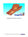
Figure 2.2: Segmentation perspective consisting of the Data Manager view and the Segmentation view
If you wonder what segmentations are good for, we shortly revisit the concept of a segmentation here. A
CT or MR image is made up of volume of physical measurements (volume elements are called voxels). In
CT images, for example, the gray value of each voxel corresponds to the mass absorbtion coefficient for
X-rays in this voxel, which is similar in many parts of the human body. The gray value does not contain
any further information, so the computer does not know whether a given voxel is part of the body or the
background, nor can it tell a brain from a liver. However, the distinction between a foreground and a
background structure is required when:
• you want to know the volume of a given organ (the computer needs to know which parts of the image
belong to this organ)
• you want to create 3D polygon visualizations (the computer needs to know the surfaces of structures
that should be drawn)
• as a necessary pre-processing step for therapy planning, therapy support, and therapy monitoring
Creating this distinction between foreground and background is called segmentation. The Segmentation
perspective of MITKApp uses a voxel based approach to segmentation, i.e. each voxel of an image must
be completely assigned to either foreground or background. This is, in contrast to some other applications
which might use an approach based on contours, where the border of a structure might cut a voxel into two
parts.
Generated on Thu Nov 3 17:31:07 2011 for DI_App_docu by Doxygen
6
The Segmentation Module
The remainder of this document will summarize the features of the Segmentation perspective and how they
are used.
2.2
Technical Issues
The Segmentation perspective makes a number of assumptions. To know what this module can be used for,
it will help you to know that:
• Images must be 2D, 3D, or 3D+t
• Images must be single-values, i.e. CT, MRI or "normal" ultrasound. Images from color doppler or
photographic (RGB) images are not supported
• Segmentations are handled as binary images of the same extent as the original image
2.3
Image Selection
The Segmentation perspective makes use of the Data Manager view to give you an overview of all images
and segmentations.
Generated on Thu Nov 3 17:31:07 2011 for DI_App_docu by Doxygen
2.4 Manual Contouring
7
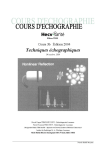
Figure 2.3: Data Manager is used for selecting the current segmentation. The reference image is selected
in the drop down box of the control area.
To select the reference image (e.g. the original CT/MR image) use the drop down box in the control area
of the Segmentation view. The segmentation image selected in the Data Manager is displayed below the
drop down box. If no segmentation image exists or none is selected create a new segmentation image by
using the "New segmentation" button. Some items of the graphical user interface might be disabled when
no image is selected. In any case, the application will give you hints if a selection is needed.
2.4
Manual Contouring
With manual contouring you define which voxels are part of the segmentation and which are not. This
allows you to create segmentations of any structeres that you may find in an image, even if they are not part
of the human body. You might also use manual contouring to correct segmentations that result from suboptimal automatic methods. The drawback of manual contouring is that you might need to define contours
on many 2D slices. However, this is moderated by the interpolation feature, which will make suggestions
for a segmentation.
Generated on Thu Nov 3 17:31:07 2011 for DI_App_docu by Doxygen
8
2.4.1
The Segmentation Module
Creating New Segmentations
Unless you want to edit existing segmentations, you have to create a new, empty segmentation before you
can edit it. To do so, click the "New manual segmentation" button. Input fields will appear where you can
choose a name for the new segmentation and a color for its display. Click the checkmark button to confirm
or the X button to cancel the new segmentation. Notice that the input field suggests names once you start
typing and that it also suggests colors for known organ names. If you use names that are not yet known to
the application, it will automatically remember these names and consider them the next time you create a
new segmentation.
Once you created a new segmentation, you can notice a new item with the "binary mask" icon in the Data
Manager tree view. This item is automatically selected for you, allowing you to start editing the new
segmentation right away.
2.4.2
Selecting Segmentations for Editing
As you might want to have segmentations of multiple structures in a single patient image, the application
needs to know which of them to use for editing. You select a segmenation by clicking it in the tree view of
Data Manager. Note that segmentations are usually displayed as sub-items of "their" patient image. In the
rare case, where you need to edit a segmentation that is not displayed as a a sub-item, you can click both
the original image AND the segmentation while holding down CTRL on the keyboard.
When a selection is made, the Segmentation View will hide all but the selected segmentation and the
corresponding original image. When there are multiple segmentations, the unselected ones will remain
in the Data Manager, you can make them visible at any time by selecting them. If you want to see all
segmenations at the same time, just clear the selection by clicking outside all the tree items in the Data
Manager.
2.4.3
Selecting Editing Tools
If you are familiar with MITKApp, you know that clicking and moving the mouse in any of the 2D render
windows will move around the crosshair that defines what part of the image is displayed. This behavior
is disabled while any of the manual segmentation tools are active -- otherwise you might have a hard time
concentrating on the contour you are drawing.
To start using one of the editing tools, click its button the the displayed toolbox. The selected editing tool
will be active and its corresponding button will stay pressed until you click the button again. Selecting a
different tool also deactivates the previous one.
If you have to delineate a lot of images, you should try using shortcuts to switch tools. Just hit the first
letter of each tool to activate it (A for Add, S for Subtract, etc.).
2.4.4
Using Editing Tools
All of the editing tools work by the same principle: you use the mouse (left button) to click anywhere in
a 2D window (any of the orientations transversal, sagittal, or frontal), move the mouse while holding the
mouse button and release to finish the editing action. All tools work on the original slices of the patient
image, i.e. with some rotated/tilted MR image volumes you need to perform a "reinit" option in the Data
Manger before you are able to use the editing tools.
Multi-step undo and redo is fully supported by all editing tools. Use the application-wide undo button in
the toolbar to revert erroneous actions.
Generated on Thu Nov 3 17:31:07 2011 for DI_App_docu by Doxygen
2.4 Manual Contouring
9
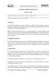
Figure 2.4: Add and Subtract Tools
Use the left mouse button to draw a closed contour. When releasing the mouse button, the contour will be
added (Add tool) to or removed from (Subtract tool) the current segmentation. Hold down the CTRL key
to invert the operation (this will switch tools temporarily to allow for quick corrections).
Figure 2.5: Paint and Wipe Tools
Use the slider below the toolbox to change the radius of these round paintbrush tools. Move the mouse in
any 2D window and press the left button to draw or erase pixels. As the Add/Subtract tools, holding CTRL
while drawing will invert the current tool’s behavior.
Figure 2.6: Region Growing Tool
Click at one point in a 2D slice widget to add an image region to the segmentation with the region growing
tool. Moving up the cursor while holding the left mouse button widens the range for the included grey
values; moving it down narrows it. When working on an image with a high range of grey values, the
selection range can be influenced more strongly by moving the cursor at higher velocity.
Region Growing selects all pixels around the mouse cursor that have a similar gray value as the pixel below
the mouse cursor. This enables you to quickly create segmentations of structures that have a good contrast
to surrounding tissue, e.g. the lungs. The tool will select more or less pixels (corresponding to a changing
gray value interval width) when you move the mouse up or down while holding down the left mouse button.
A common issue with region growing is the so called "leakage" which happens when the structure of
interest is connected to other pixels, of similar gray values, through a narrow "bridge" at the border of the
structure. The Region Growing tool comes with a "leakage detection/removal" feature. If leakage happens,
you can left-click into the leakage region and the tool will try to automatically remove this region (see
illustration below).
Generated on Thu Nov 3 17:31:07 2011 for DI_App_docu by Doxygen
10
The Segmentation Module
Figure 2.7: Leakage correction feature of the Region Growing tool
Figure 2.8: Correction Tool
You do not have to draw a closed contour to use the Correction tool and do not need to switch between the
Add and Substract tool to perform small corrective changes. The following figure shows the usage of this
tool:
• if the user draws a line which starts and ends outside the segmenation a part of it is cut off (left
image)
• if the line is drawn fully inside the segmentation the marked region is added to the segmentation
(right image)
Generated on Thu Nov 3 17:31:07 2011 for DI_App_docu by Doxygen
2.4 Manual Contouring
11
Figure 2.9: Actions of the Correction tool illustrated.
Figure 2.10: Fill Tool
Left-click inside a segmentation with holes to completely fill all holes.
Figure 2.11: Erase Tool
This tool removes a connected part of pixels that form a segmentation. You may use it to remove so called
islands (see picture) or to clear a whole slice at once (hold CTRL while clicking).
2.4.5
Interpolation
Creating segmentations for modern CT volumes is very time-consuming, because strucutres of interest can
easily cover a range of 50 or more slices. The Segmentation view offers a helpful feature for these cases:
Generated on Thu Nov 3 17:31:07 2011 for DI_App_docu by Doxygen
12
The Segmentation Module
"Interpolation" creates suggestions for a segmentation whenever you have a slice that
• has got neighboring slices with segmentations (these do not need to be direct neighbors but could
also be a couple of slices away) AND
• is completely clear of a manual segmentation -- i.e. there will be no suggestion if there is even only
a single pixel of segmentation in the current slice.
Interpolated suggestions are displayed in a different way than manual segmentations are, until you "accept"
them as part of the segmentation. To accept single slices, click the "Accept" button below the toolbox. If
you have segmented a whole organ in every-x-slice, you may also review the interpolations and then accept
all of them at once by clicking "... all slices".
2.5
Organ Segmentation
The manual contouring described above is a fallback option that will work for any kind of images and
structures of interest. However, manual contouring is very time-consuming and tedious. This is why a major part of image analysis research is working towards automatic segmentation methods. The Segmentation
View comprises a number of easy-to-use tools for segmentation of CT images (Liver) and MR image (left
ventricle and wall, left and right lung).
2.5.1
Liver on CT Images
On CT image volumes, preferrably with a contrast agent in the portal venous phase, the Liver tool will fully
automatically analyze and segment the image. All you have to do is to load and select the image, then click
the "Liver" button. During the process, which takes a minute or two, you will get visual progress feedback
by means of a contour that moves closer and closer to the real liver boundaries.
2.5.2
Heart, Lung, and Hippocampus on MRI
While liver segmentation is performed fully automatic, the following tools for segmentation of the heart,
the lungs, and the hippocampus need a minimum amount of guidance. Click one of the buttons on the
"Organ segmentation" page to add an average model of the respective organ to the image. This model can
be dragged to the right position by using the left mouse button while holding down the CTRL key. You can
also use CTRL + middle mouse button to rotate or CTRL + right mouse button to scale the model.
Before starting the automatic segmentation process by clicking the "Start segmentation" button, try placing
the model closely to the organ in the MR image (in most cases, you do not need to rotate or scale the
model). During the segmentation process, a green contour that moves closer and closer to the real liver
boundaries will provide you with visual feedback of the segmentation progress.
The algorithms used for segmentation of the heart and lung are method which need training by a number
of example images. They will not work well with other kind of images, so here is a list of the image types
that were used for training:
• Hippocampus segmentation: T1-weighted MR images, 1.5 Tesla scanner (Magnetom Vision,
Siemens Medical Solutions), 1.0 mm isotropic resolution
• Heart: Left ventricle inner segmentation (LV Model): MRI; velocity encoded cine (VEC-cine) MRI
sequence; trained on systole and diastole
• Heart: Left ventricular wall segmentation (LV Inner Wall, LV Outer Wall): 4D MRI; short axis 12
slice spin lock sequence(SA_12_sl); trained on whole heart cycle
Generated on Thu Nov 3 17:31:07 2011 for DI_App_docu by Doxygen
2.6 Lesion Segmentation
13
• Lung segmentation: 3D and 4D MRI; works best on FLASH3D and TWIST4D sequences
2.5.3
Other Organs
As mentioned in the Heart/Lung section, most of the underlying methods are based on "training". The
basic algorithm is versatile and can be applied on all kinds of segmentation problems where the structure
of interest is topologically like a sphere (and not like a torus etc.). If you are interested in other organs than
those offered by the current version of the Segmentation view, please contact our research team.
2.6
Lesion Segmentation
Lesion segmentation is a little different from organ segmentation. Since lesions are not part of the healthy
body, they sometimes have a diffused border, and are often found in varying places all over the body. The
tools in this section offer efficient ways to create 3D segmentations of such lesions.
The Segmentation View currently offers supoprt for enlarged lymph nodes.
To segment an enlarged lymph node, find a more or less central slice of it, activate the "Lymph Node"
tool and draw a rough contour on the inside of the lymph node. When releaseing the mouse button, a
segmentation algorithm is started in a background task. The result will become visible after a couple of
seconds, but you do not have to wait for it. If you need to segment several lymph nodes, you can continue
to inspect the image right after closing the drawn contour.
If the lymph node segmentation is not to your content, you can select the "Lymph Node Correction" tool
and drag parts of the lymph node surface towards the right position (works in 3D, not slice-by-slice). This
kind of correction helps in many cases. If nothing else helps, you can still use the pure manual tools as a
fallback.
2.7
Things you can do with segmentations
As mentioned in the introduction, segmentations are never an end in themselves. Consequently, the Segmentation view adds a couple of "post-processing" actions to the Data Manager. These actions are accessible through the context-menu of segmentations in Data Manager’s list view
Generated on Thu Nov 3 17:31:07 2011 for DI_App_docu by Doxygen
14
The Segmentation Module
Figure 2.12: Context menu items for segmentations.
• Create polygon model applies the marching cubes algorithms to the segmentation. This polygon
model can be used for visualization in 3D or other things such as stereolithography (3D printing).
• Create smoothed polygon model uses smoothing in addition to the marching cubes algorithms,
which creates models that do not follow the exact outlines of the segmentation, but look smoother.
• Statistics goes through all the voxels in the patient image that are part of the segmentation and calculates some statistical measures (minumum, maximum, median, histogram, etc.). Note that the
statistics are ALWAYS calculated for the parent element of the segmentation as shown in Data Manager.
• Autocrop can save memory. Manual segmentations have the same extent as the patient image, even
if the segmentation comprises only a small sub-volume. This invisible and meaningless margin is
removed by autocropping.
2.8
Surface Masking
You can use the surface masking tool to create binary images from a surface which is used used as a mask
on an image. This task is demonstrated below:
Generated on Thu Nov 3 17:31:07 2011 for DI_App_docu by Doxygen
2.9 Technical Information for Developers
15
Figure 2.13: Load an image and a surface. Select the image and the surface in the corresponding drop-down
boxes (both are selected automatically if there is just one image and one surface)
Figure 2.14: After clicking "Create segmentation from surface" the newly created binary image is inserted
in the DataManager and can be used for further processing
2.9
Technical Information for Developers
For technical specifications see Technical design of QmitkSegmentation and for information on the extensions of the tools system How to extend the Segmentation bundle with external tools .
Generated on Thu Nov 3 17:31:07 2011 for DI_App_docu by Doxygen
16
The Segmentation Module
2.10
Technical design of QmitkSegmentation
• Introduction
• Overview of tasks
• Classes involved
2.10.1
Introduction
QmitkSegmentation was designed for the liver resection planning project "ReLiver". The goal was a stable,
well-documented, extensible, and testable re-implementation of a functionality called "ERIS", which was
used for manual segmentation in 2D slices of 3D or 3D+t images. Re-implementation was chosen because
it seemed to be easier to write documentation and tests for newly developed code. In addition, the old code
had some design weaknesses (e.g. a monolithic class), which would be hard to maintain in the future.
By now Segmentation is a well tested and easily extensible vehicle for all kinds of interactive segmentation
applications. A separate page describes how you can extend Segmentation with new tools in a shared object
(DLL): How to extend the Segmentation bundle with external tools.
2.10.2
Overview of tasks
We identified the following major tasks:
1. Management of images: what is the original patient image, what images are the active segmentations?
2. Management of drawing tools: there is a set of drawing tools, one at a time is active, that is,
someone has to decide which tool will receive mouse (and other) events.
3. Drawing tools: each tool can modify a segmentation in reaction to user interaction. To do so, the
tools have to know about the relevant images.
4. Slice manipulation: drawing tools need to have means to extract a single slice from an image volume
and to write a single slice back into an image volume.
5. Interpolation of unsegmented slices: some class has to keep track of all the segmentations in a
volume and generate suggestions for missing slices. This should be possible in all three orthogonal
slice direction.
6. Undo: Slice manipulations should be undoable, no matter whether a tool or the interpolation mechanism changed something.
7. GUI: Integration of everything.
2.10.3
Classes involved
The above blocks correspond to a number of classes. Here is an overview of all related classes with their
responsibilities and relations:
Generated on Thu Nov 3 17:31:07 2011 for DI_App_docu by Doxygen
2.10 Technical design of QmitkSegmentation
17
1. Management of images: mitk::ToolManager has a set of reference data (original images) and a
second set of working data (segmentations). mitk::Tool objects know a ToolManager and can ask
the manager for the currently relevant images. There are two GUI elements that enable the user to
modify the set of reference and working images (QmitkToolReferenceDataSelectionBox and QmitkToolWorkingDataSelectionBox). GUI and non-GUI classes are coupled by itk::Events (non-GUI to
GUI) and direct method calls (GUI to non-GUI).
2. Management of drawing tools: As a second task, ToolManager manages all available tools and
makes sure that one at a time is able to receive MITK events. The GUI for selecting tools is implemented in QmitkToolSelectionBox.
3. Drawing tools: Drawing tools all inherit from mitk::Tool, which is a mitk::StateMachine. There is
a number of derivations from Tool, each offering some helper methods for specific sub-classes, like
manipulation of 2D slices. Tools are instantiated through the itk::ObjectFactory, which means that
there is also one factory for each tool (e.g. mitk::AddContourToolFactory). For the GUI representation, each tool has an identification, consisting of a name and an icon (XPM). The actual drawing
methods are mainly implemented in mitk::SegTool2D (helper methods) and its sub-classes for region
growing, freehand drawing, etc.
4. Slice manipulation: There are two filters for manipulation of slices inside a 3D image volume.
mitk::ExtractImageFilter retrieves a single 2D slice from a 3D volume.
mitk::OverwriteSliceImageFilter replaces a slice inside a 3D volume with a second slice which is
a parameter to the filter. These classes are used extensively by most of the tools to fulfill their task.
mitk::OverwriteSliceImageFilter cooperates with the interpolation classes to inform them of single
slice modifications.
5. Interpolation of unsegmented slices: There are two classes involved in interpolation:
mitk::SegmentationInterpolationController knows a mitk::Image (the segmentation) and scans its
Generated on Thu Nov 3 17:31:07 2011 for DI_App_docu by Doxygen
18
The Segmentation Module
contents for slices with non-zero pixels. It keeps track of changes in the image and is always able to
tell, which neighbors of a slice (in the three orthogonal slice directions) contain segmentations. The
class also performs this interpolation for single slices on demand. Again, we have a second class
responsible for the GUI: QmitkSlicesInterpolator enables/disables interpolation and offers to accept
interpolations for one or all slices.
6. Undo: Undo functionality is implemented in mitk::OverwriteSliceImageFilter, since this is the central place where all image modifications are made. The filter stores a binary difference image to the
undo stack as a mitk::ApplyDiffImageOperation. When the user requests undo, this ApplyDiffImageOperation will be executed by a singleton class DiffImageApplier. The operation itself observes
the image, which it refers to, for itk::DeleteEvent, so no undo operation will be executed on/for
images that have already been destroyed.
7. GUI: The top-level GUI is the functionality QmitkSegmentation, which is very thin in comparison to
ERIS. There are separate widgets for image and tool selection, for interpolation. Additionaly, there
are some methods to create, delete, crop, load and save segmentations.
2.11
How to extend the Segmentation bundle with external tools
• Introduction
• What might be part of an extension
– Tool classes
– GUI classes for tools
– Additional files
• Writing a CMake file for a tool extension
• Compiling the extension
• Configuring ITK autoload
2.11.1
Introduction
The application for manual segmentation in MITK (Segmentation bundle) comes with a tool class framework that is extensible with new tools (description at Technical design of QmitkSegmentation). The usual
way to create new tools (since it is mostly used inside DKFZ) is to just add new files to the MITK source
code tree. However, this requires to be familiar with the MITK build system and turnaround time during
development might be long (recompiling parts of MITK again and again).
For external users who just want to use MITK as a library and application, there is a way to create new
segmentation tools in an MITK external project, which will compile the new tools into a shared object
(DLL). Such shared objects can be loaded via the ITK object factory and its autoload feature on application
startup. This document describes how to build such external extensions.
Example files can be found in the MITK source code in the directory ${MITK_SOURCE_DIR}/QApplications/ToolExtensionsExample/.
2.11.2
What might be part of an extension
The extension concept assumes that you want to create one or several new interactive segmentation tools
for Segmentation or another MITK functionality that uses the tools infrastructure. In the result you will
create a shared object (DLL), which contains several tools and their GUI counterparts, plus optional code
that your extension requires. The following sections shortly describe each of these parts.
Generated on Thu Nov 3 17:31:07 2011 for DI_App_docu by Doxygen
2.11 How to extend the Segmentation bundle with external tools
2.11.2.1
19
Tool classes
A tool is basically any subclass of mitk::Tool. Tools are created at runtime through the ITK object factory
(so they inherit from itk::Object). Tools should handle the interaction part of a segmentation method,
i.e. create seed points, draw contours, etc., in order to parameterize segmentation algorithms. Simple
algorithms can even be part of a tool. A tools is identified by icon (XPM format), name (short string) and
optionally a group name (e.g. the group name for Segmentation is "default").
There is a naming convention: you should put a tool called mitk::ExternalTool into files called
mitkExternalTool.h and mitkExternalTool.cpp. This is required if you use the convenience macros described below, because there need to be ITK factories, which names are directly derived
from the file names of the tools. For the example of mitk::ExternalTool there would be a factory called
mitk::ExternalToolFactory in a file named mitkExternalToolFactory.cpp.
2.11.2.2
GUI classes for tools
Tools are non-graphical classes that only implement interactions in renderwindows. However, some tools
will need a means to allow the user to set some parameters -- a graphical user interface, GUI. In the Qt3
case, tool GUIs inherit from QmitkToolGUI, which is a mixture of QWidget and itk::Object. Tool GUIs
are also created through the ITK object factory.
Tools inform their GUIs about state changes by messages. Tool GUIs communicate with their associated
tools via direct method calls (they know their tools). See mitk::BinaryThresholdTool for examples.
Again a naming convention:
if the convenience macros for tool extension
jects are used, you have to put a tool GUI called QmitkExternalToolGUI
named QmitkExternalToolGUI.cpp and QmitkExternalToolGUI.h. The
macro will create a factory called QmitkExternalToolGUIFactory into a
QmitkExternalToolGUIFactory.cpp.
2.11.2.3
shared obinto a files
convenience
file named
Additional files
If you are writing tools MITK externally, these tools might depend on additional files, e.g. segmentation
algorithms. These can also be compiled into a tool extension shared object.
2.11.3
Writing a CMake file for a tool extension
Summing up the last section, an example tool extension could comprise the following files:
mitkExternalTool.h
mitkExternalTool.xpm
mitkExternalTool.cpp
\
>--- implementing mitk::ExternalTool (header, icon, implementation)
/
QmitkExternalToolGUI.h
,-- implementing a GUI for mitk::ExternalTool
QmitkExternalToolGUI.cpp /
externalalgorithm.h
\
externalalgorithm.cpp
\
externalalgorithmsolver.h
>-- a couple of files (not related to MITK tools)
externalalgorithmsolver.cpp /
This should all be compiled into one shared object. Just like ITK, VTK and MITK we will use CMake for
this purpose (I assume you either know or are willing to learn about www.cmake.org) A CMake file for
the above example would look like this:
Generated on Thu Nov 3 17:31:07 2011 for DI_App_docu by Doxygen
20
The Segmentation Module
PROJECT ( ExternalTool )
FIND_PACKAGE(ITK)
FIND_PACKAGE(MITK)
FIND_PACKAGE(Qt3)
ADD_DEFINITIONS(${QT_DEFINITIONS})
SET( TOOL_QT3GUI_FILES
QmitkExternalToolGUI.cpp
)
SET( TOOL_FILES
mitkExternalTool.cpp
)
SET( TOOL_ADDITIONAL_CPPS
externalalgorithm.cpp
externalalgorithmsolver.cpp
)
SET( TOOL_ADDITIONAL_MOC_H
)
MITK_GENERATE_TOOLS_LIBRARY(mitkExternalTools)
Basically, you only have to change the definitions of TOOL_FILES and, optionally, TOOL_QT3GUI_FILES, TOOL_ADDITIONAL_CPPS and TOOL_ADDITIONAL_MOC_H. For all .cpp files in TOOL_FILES and TOOL_QT3GUI_FILES there will be factories created assuming the naming conventions
described in the sections above. Files listed in TOOL_ADDITIONAL_CPPS will just be compiled. Files
listed in TOOL_ADDITIONAL_MOC_H will be run through Qts meta object compiler moc -- this is neccessary for all objects that have the Q_OBJECT macro in their declaration. moc will create new files that
will also be compiled into the library.
2.11.4
Compiling the extension
For compiling a tool extension, you will need a compiled version of MITK. We will assume MITK was
compiled into /home/user/mitk/debug. You need to build MITK with BUILD_SHARED_CORE turned
on!
You build the tool extension just like any other CMake based project:
• know where your source code is (e.g. /home/user/mitk/tool-extension-src)
• change into the directory, where you want to compile the shared object (e.g. /home/user/mitk/toolextension-debug)
• invoke cmake: ccmake /home/user/mitk/tool-extension-src
• configure (press c or the "configure" button)
• set the ITK_DIR variable to the directory, where you compiled ITK
• set the MITK_DIR variable
/home/user/mitk/debug
to
the
directory,
where
you
compiled
MITK:
• configure (press "c" or the "configure" button)
• generate (press "g" or the "generate" button)
This should do it and leave you with a or project file or Makefile that you can compile (using make or
VisualStudio).
Generated on Thu Nov 3 17:31:07 2011 for DI_App_docu by Doxygen
2.11 How to extend the Segmentation bundle with external tools
2.11.5
21
Configuring ITK autoload
If the compile succeeds, you will get a library mitkExternalTools.dll or libmitkExternalTools.so. This
library exports a symbol itkLoad which is expected by the ITK object factory.
On application startup the ITK object factory will search a list of directories from the environment variable ITK_AUTOLOAD_PATH. Set this environment variable to your binary directory
(/home/user/mitk/tool-extension-debug).
The ITK object factory will load all shared objects that it finds in the specified directories and will
test if they contain a symbol (function pointer) itkLoad, which is expected to return a pointer to a
itk::ObjectFactoryBase instance. If such a symbol is found, the returned factory will be registered with the
ITK object factory.
If you successfully followed all the steps above, MITK will find your mitk::ExternalTool on application
startup, when the ITK object factory is asked to create all known instances of mitk::Tool. Furthermore, if
your mitk::ExternalTool claims to be part of the "default" group, there will be a new icon in Segmentation,
which activates your tool.
Have fun! (And Windows users: welcome to the world of DLLs)
Generated on Thu Nov 3 17:31:07 2011 for DI_App_docu by Doxygen
22
The Segmentation Module
Generated on Thu Nov 3 17:31:07 2011 for DI_App_docu by Doxygen
Chapter 3
The Brain Network Analysis Module
24
The Brain Network Analysis Module
Figure 3.1: Icon of the Module
3.1
Summary
This module can be used to create a network from a parcellation and a fiber image as well as to calculate
and display network statistics.
This document will tell you how to use this module, but it is assumed that you already know how to use
MITK in general.
Please see Details for more detailed information on usage and supported filters. If you encounter problems
using the module, please have a look at the Troubleshooting page.
3.2
Details
Manual sections:
• Overview
• Usage
• Troubleshooting
3.3
Overview
This module is currently under heavy development and as such the interface as well as the capabilities are
likely to change significantly between different versions.
This documentation describes the features of this current version.
Generated on Thu Nov 3 17:31:07 2011 for DI_App_docu by Doxygen
3.3 Overview
25
Figure 3.2: The interface
Generated on Thu Nov 3 17:31:07 2011 for DI_App_docu by Doxygen
26
The Brain Network Analysis Module
3.4
Usage
To create a network select first a parcellation of the brain (e.g. as provided by freesurfer ) by
CTRL+Leftclick and secondly a fiber image ( as created using tractography module). Then click on the
"Create Network" button.
To calculate network statistics select a network in the datamanager. At this time the following statistics are
calculated for the entire network:
• The number of vertices in the network
• The number of edges in the network
• The number of edges which have the same vertex as beginning and end point
• The average degree of the nodes in the network
• The connection density the network (the number of edges divided by the number of possible edges)
• The unweighted efficiency of the network ( 1 divided by average path length, this is zero for disconnected graphs)
Furthermore some statistics are calculated on a per node basis and displayed as histograms:
• The degree of each node
• The (unweighted) betweenness centrality of each node
• The spread of shortest paths between each pair of nodes (For disconnected graphs the shortest paths
with infinite length are omitted for readability)
3.5
Troubleshooting
No known problems.
All other problems.
Please report to the MITK mailing list. See http://www.mitk.org/wiki/Mailinglist on how
to do this.
Generated on Thu Nov 3 17:31:07 2011 for DI_App_docu by Doxygen
Chapter 4
The DataManager
28
The DataManager
Figure 4.1: Icon of the Module
4.1
Introduction
The Datamanager is the central componenent to manage medical data like images, surfaces, etc.. After
loading one or more data into the Datamanager the data are shown in the four-view window, the so called
Standard View. The user can now start working on the data by just clicking into the standard view or by
using the MITK-modules such as "Segmentation" or "Basic Image Processing".
Available sections:
• Introduction
• Loading Data
• Saving Data
• Working with the Datamanager
– List of Data-Elements
– Visibility of Data-Elements
– Representation of Data-Elements
– Preferences
• Property List
Generated on Thu Nov 3 17:31:07 2011 for DI_App_docu by Doxygen
4.2 Loading Data
29
Figure 4.2: How MITK looks when starting
4.2
Loading Data
There are three ways of loading data into the Datamanager as so called Data-Elements.
The user can just drag and drop data into the Datamanager or directly into one of the four parts of the
Standard View. He can as well use the Open-Button in the right upper corner. Or he can use the standard
"File->Open"-Dialog on the top.
A lot of file-formats can be loaded into MITK, for example
• 2D-images/3D-volumes with or without several timesteps (∗.dcm, ∗.ima, ∗.pic, ...)
• Surfaces (∗.stl, ∗.vtk, ...)
• Pointsets (∗.mps)
• ...
The user can also load a series of 2D images (e.g. image001.bmp, image002.bmp ...) to a MITK 3D
volume. To do this, just drag and drop one of those 2D data files into the Datamanager by holding the ALT
key.
After loading one or more data into the Datamanager they appear as Data-Elements in a sorted list inside
the Datamanager. Data-Elements can also be sorted hierarchically as a parent-child-relation. For example
Generated on Thu Nov 3 17:31:07 2011 for DI_App_docu by Doxygen
30
The DataManager
after using the Segmentation-Module on Data-Element1 the result is created as Data-Element2, which is a
child of Data-Element1 (see Screenshot1). The order can be changed by drag and drop.
Figure 4.3: Screenshot1
The listed Data-Elements are shown in the standard view. Here the user can scale or rotate the medical
objects or he can change the cutting planes of the object by just using the mouse inside this view.
4.3
Saving Data
There are two ways of saving data from the Datamanger. The user can either save the whole project
with all Data-Elements by clicking on "File"->"Save Project" or he can save single Data-Elements by
right-clicking->"Save", directly on a Data-Element. When saving the whole project, the sorting of DataElements is saved as well. By contrast the sorting is lost, when saving a single Data-Element.
4.4
4.4.1
Working with the Datamanager
List of Data-Elements
The Data-Elements are listed in the Datamanager. As described above the elements can be sorted hierarchically as a parent-child-relation. For example after using the Segmentation-Module on Data-Element1
the result is created as Data-Element2, which is a child of Data-Element1 (see Screenshot1). By drag and
drop the sorting of Data-Elements and their hierarchical relation can be changed.
4.4.2
Visibility of Data-Elements
By default all loaded Data-Elements are visible in the standard view. The visibility can be changed by
right-clicking on the Data-Element and then choosing "Toogle visibility". The box in front of the DataElement in the Datamanager shows the visibility. A green-filled box means a visible Data-Element, an
empty box means an invisible Data-Element (see Screenshot1).
Generated on Thu Nov 3 17:31:07 2011 for DI_App_docu by Doxygen
4.4 Working with the Datamanager
4.4.3
31
Representation of Data-Elements
There are different types of representations how to show the Data-Element inside the standard view. By
right-clicking on the Data-Element all options are listed (see Screenshot2 and Screenshot 3).
• An arbitrary color can be chosen
• The opacity can be changed with a slide control
• In case of images a texture interpolation can be switched on or off. The texture interpolation
smoothes the image, so that no single pixels are visible anymore.
• In case of surfaces the surface representation can be changed between points, wireframe or surface.
• Global reinit updates all windows to contain all the current data. Reinit updates a single data item
fits the windows to contain this data item.
Figure 4.4: Screenshot2: Properties for images
Generated on Thu Nov 3 17:31:07 2011 for DI_App_docu by Doxygen
32
The DataManager
Figure 4.5: Screenshot3: Properties for surfaces
4.4.4
Preferences
For the datamanager there are already some default hotkeys like the del-key for deleting a Data-Element.
The whole list is seen in Screenshot4. From here the Hotkeys can also be changed. The preference page is
found in "Window"->"Preferences".
Generated on Thu Nov 3 17:31:07 2011 for DI_App_docu by Doxygen
4.5 Property List
33
Figure 4.6: Screenshot4
4.5
Property List
The Property List displays all the properties the currently selected Data-Element has. Which properties
these are depends on the Data-Element. Examples are opacity, shader, visibility. These properties can be
changed by clicking on the appropriate field in the "value" column.
Generated on Thu Nov 3 17:31:07 2011 for DI_App_docu by Doxygen
34
The DataManager
Figure 4.7: Screenshot5: Property List
Generated on Thu Nov 3 17:31:07 2011 for DI_App_docu by Doxygen
Chapter 5
General MITK Manual
36
General MITK Manual
Welcome to the basic MITK user manual. This document tries to give a concise overview of the basic
functions of MITK and be an comprehensible guide on using them.
Available sections:
• About MITK
• The User Interface
• Perspectives
5.1
About MITK
MITK is an open-source framework that was originally developed as a common framework for Ph.D.
students in the Division of Medical and Biological Informatics (MBI) at the German Cancer Research
Center. MITK aims at supporting the development of leading-edge medical imaging software with a high
degree of interaction.
MITK re-uses virtually anything from VTK and ITK. Thus, it is not at all a competitor to VTK or ITK,
but an extension, which tries to ease the combination of both and to add features not supported by VTK or
ITK.
Research institutes, medical professionals and companies alike can use MITK as a basic framework for
their research and even commercial (thorough code research needed) software due to the BSD-like software
license.
Research institutes will profit from the high level of integration of ITK and VTK enhanced with data
management, advanced visualization and interaction functionality in a single framework that is supported
by a wide variety of researchers and developers. You will not have to reinvent the wheel over and over and
can concentrate on your work.
Medical Professionals will profit from MITK and the MITK applications by using its basic functionalities
for research projects. But nonetheless they will be better off, unless they are programmers themselves, to
cooperate with a research institute developing with MITK to get the functionalitiy they need. MITK and
the MITK applications are not certified medical products and may be used in a research setting only. They
must not be used in patient care.
5.2
The User Interface
The layout of the MITK applications is designed to give a clear distinction between the different work
areas. The following figure gives an overview of the main sections of the user interface.
Generated on Thu Nov 3 17:31:07 2011 for DI_App_docu by Doxygen
5.3 Four Window View
37
Figure 5.1: The Common MITK Application Graphical User Interface
The datamanager and the Perspectives have their own help sections. This document explains the use of:
• The Four Window View
• The Menu
• The Levelwindow
• The System Load Indicator
5.3
5.3.1
Four Window View
Overview
The four window view is the heart of the MITK image viewing. The standard layout is three 2D windows
and one 3D window, with the transversal window in the top left quarter, the sagittal window in the top right
quarter, the coronal window in the lower left quarter and the 3D window in the lower right quarter. The
different planes form a crosshair that can be seen in the 3D window.
Once you select a point within the picture, informations about it are displayed at the bottom of the screen.
5.3.2
Navigation
Left click in any of the 2D windows centers the crosshair on that point. Pressing the right mouse button and
moving the mouse zooms in and out. By scrolling with the mouse wheel you can navigate through the
slices of the active window and pressing the mouse wheel while moving the mouse pans the image section.
Generated on Thu Nov 3 17:31:07 2011 for DI_App_docu by Doxygen
38
General MITK Manual
In the 3D window you can rotate the object by pressing the left mouse button and moving the mouse,
zoom either with the right mouse button as in 2D or with the mouse wheel, and pan the object by moving
the mouse while the mouse wheel is pressed. Placing the cursor within the 3D window and holding the "F"
key allows free flight into the 3D view.
5.3.3
Customizing
By moving the cursor to the upper right corner of any window you can activate the window menu. It
consists of three buttons.
Figure 5.2: Crosshair
The crosshair button allows you toggle the crosshair, reset the view and change the behaviour of the planes.
Generated on Thu Nov 3 17:31:07 2011 for DI_App_docu by Doxygen
5.4 Menu
39
Activating either of the rotation modes allows you to rotate the planes visible in a 2D window by moving
the mouse cursor close to them and click and dragging once it changes to indicate that rotation can be done.
The swivel mode is recommended only for advanced users as the planes can be moved freely by clicking
and dragging anywhere within a 2D window.
The middle button expands the corresponding window to fullscreen within the four window view.
Figure 5.3: Layout Choices
The right button allows you to choose between many different layouts of the four window view to use the
one most suited to your task.
5.4
5.4.1
Menu
File
This dialog allows you to save, load and clear entire projects, this includes any nodes in the data manager.
5.4.2
Edit
This dialog supports undo and redo operations as well as the image navigator, which gives you sliders to
navigate through the data quickly.
The Preferences dialog allows you to adjust and save your custom settings.
Generated on Thu Nov 3 17:31:07 2011 for DI_App_docu by Doxygen
40
5.4.3
General MITK Manual
Help
This dialog contains this help, the welcome screen and information about MITK Diffusion.
5.5
Levelwindow
Once an image is loaded the levelwindow appears to the right hand side of the four window view. With
this tool you can adjust the range of grey values displayed and the gradient between them. Moving the
lower boundary up results in any pixels having a value lower than that boundary to be displayed as black.
Lowering the upper boundary causes all pixels having a value higher than it to be displayed as white.
The pixels with a value between the lower and upper boundary are displayed in different shades of grey.
This way a smaller levelwindow results in higher contrasts while cutting of the information outside its
range whereas a larger levelwindow displays more information at the cost of contrast and detail.
You can pick the levelwindow with the mouse to move it up and down, while moving the mouse cursor to
the left or right to change its size. Picking one of the boundaries with a left click allows you to change the
size symmetrically. Holding CTRL and clicking a boundary adjusts only that value.
5.6
System Load Indicator
The System Load Indicator in the lower right hand corner of the screen gives information about the memory
currently required by the MITK application. Keep in mind that image processing is a highly memory
intensive task and monitor the indicator to avoid your system freezing while constantly swapping to the
hard drive.
5.7
Perspectives
The different tasks that arise in medical imaging need very different approaches. To acknowledge this
circumstance MITK supplies a framework that can be build uppon by very different solutions to those
tasks. These solutions are called perspectives, each of them works independently of others although they
might be used in sequence to achieve the solution of more difficult problems.
It is possible to switch between the perspectives using the "Window"->"Open Perspective" dialog, using
the Welcome Screen or by using the bar on top of the editor area.
See Menu for more information about switching perspectives.
Generated on Thu Nov 3 17:31:07 2011 for DI_App_docu by Doxygen
Chapter 6
MITK Diffusion Imaging (MITK-DI)
42
MITK Diffusion Imaging (MITK-DI)
This module provides means to diffusion weighted image reconstruction, visualization and quantification.
Diffusion tensors as well as different q-ball reconstruction schemes are supported. Q-ball imaging aims
at recovering more detailed information about the orientations of fibers from diffusion MRI measurements
and, in particular, to resolve the orientations of crossing fibers.
Available sections:
• Known Issues
• Preprocessing
• Tensor Reconstruction
• Q-Ball Reconstruction
• Dicom Import
• Quantification
• ODF Visualization Setting
• References
• Technical Information for Developers
Figure 6.1: The MITK Diffusion Imaging Module
Generated on Thu Nov 3 17:31:07 2011 for DI_App_docu by Doxygen
6.1 Known Issues
6.1
43
Known Issues
• Dicom Import: The dicom import has so far only been implemented for Siemens dicom images.
MITK-DI is capable of reading the nrrd format, which is documented elsewhere [1, 2]. These files
can be created by combining the raw image data with a corresponding textual header file. The file
extension should be changed from ∗.nrrd to ∗.dwi or from ∗.nhdr to ∗.hdwi respectively in order to
let MITK-DI recognize the diffusion related header information provided in the files.
6.2
Preprocessing
The preprocessing view gives an overview over the important features of a diffusion weighted image like
the number of gradient directions, b-value and the measurement frame. Additionally it allows the extraction
of the B0 image and the generation of a binary brain mask. The image volume can be modified by applying
a new mesurement frame, which is useful if the measurement frame is not set correctly in the image header,
or by averaging redundant gradient directions.
Generated on Thu Nov 3 17:31:07 2011 for DI_App_docu by Doxygen
44
MITK Diffusion Imaging (MITK-DI)
Figure 6.2: Preprocessing
6.3
Tensor Reconstruction
The tensor reconstruction view allows ITK based tensor reconstruction [3]. The advanced settings for ITK
reconstruction let you configure a manual threshold on the non-diffusion weighted image. All voxels below
this threshold will not be reconstructed and left blank. It is also possible to check for negative eigenvalues.
The according voxels are also left blank.
Generated on Thu Nov 3 17:31:07 2011 for DI_App_docu by Doxygen
6.3 Tensor Reconstruction
45
Figure 6.3: ITK tensor reconstruction
A few seconds (depending on the image size) after the reconstruction button is hit, a colored image should
appear in the main window.
Figure 6.4: Tensor image after reconstruction
The view also allows the generation of artificial diffusion weighted or Q-Ball images from the selected
tensor image. The ODFs of the Q-Ball image are directly initialized from the tensor values and afterwards
normalized. The diffusion weighted image is estimated using the l2-norm image of the tensor image as B0.
Generated on Thu Nov 3 17:31:07 2011 for DI_App_docu by Doxygen
46
MITK Diffusion Imaging (MITK-DI)
The gradient images are afterwards generated using the standard tensor equation.
6.4
Q-Ball Reconstruction
The q-ball reonstruction bundle implements a variety of reconstruction methods. The different reconstruction methods are described in the following:
• Numerical: The original, numerical q-ball reconstruction presented by Tuch et al. [5]
• Standard (SH): Descoteaux’s reconstruction based on spherical harmonic basis functions [6]
• Solid Angle (SH): Aganj’s reconstruction with solid angle consideration [7]
• ADC-profile only: The ADC-profile reconstructed with spherical harmonic basis functions
• Raw signal only: The raw signal reconstructed with spherical harmonic basis functions
Figure 6.5: The q-ball resonstruction view
B0 threshold works the same as in tensor reconstruction. The maximum l-level configures the size of the
spherical harmonics basis. Larger l-values (e.g. l=8) allow higher levels of detail, lower levels are more
stable against noise (e.g. l=4). Lambda is a regularisation parameter. Set it to 0 for no regularisation.
lambda = 0.006 has proven to be a stable choice under various settings.
Figure 6.6: Advanced q-ball reconstruction settings
Generated on Thu Nov 3 17:31:07 2011 for DI_App_docu by Doxygen
6.5 Dicom Import
47
This is how a q-ball image should initially look after reconstruction. Standard q-balls feature a relatively
low GFA and thus appear rather dark. Adjust the level-window to solve this.
Figure 6.7: q-ball image after reconstruction
6.5
Dicom Import
The dicom import does not cover all hardware manufacturers but only Siemens dicom images. MITK-DI
is also capable of reading the nrrd format, which is documented elsewhere [1, 2]. These files can be created
by combining the raw image data with a corresponding textual header file. The file extension should be
changed from ∗.nrrd to ∗.dwi or from ∗.nhdr to ∗.hdwi respectively in order to let MITK-DI recognize the
diffusion related header information provided in the files.
In case your dicom images are readable by MITK-DI, select one or more input dicom folders and click
import. Each input folder must only contain DICOM-images that can be combined into one vector-valued
3D output volume. Different patients must be loaded from different input-folders. The folders must not
contain other acquisitions (e.g. T1,T2,localizer).
In case many imports are performed at once, it is recommended to set the the optional output folder argument. This prevents the images from being kept in memory.
Generated on Thu Nov 3 17:31:07 2011 for DI_App_docu by Doxygen
48
MITK Diffusion Imaging (MITK-DI)
Figure 6.8: Dicom import
The option "Average duplicate gradients" accumulates the information that was acquired with multiple
repetitions for one gradient. Vectors do not have to be precisely equal in order to be merged, if a "blur
radius" > 0 is configured.
6.6
Quantification
The quantification view allows the derivation of different scalar anisotropy measures for the reconstructed
tensors (Fractional Anisotropy, Relative Anisotropy, Axial Diffusivity, Radial Diffusivity) or q-balls (Generalized Fractional Anisotropy).
Generated on Thu Nov 3 17:31:07 2011 for DI_App_docu by Doxygen
6.7 ODF Visualization Setting
49
Figure 6.9: Anisotropy quantification
6.7
ODF Visualization Setting
In this small view, the visualization of ODFs and diffusion images can be configured. Depending on the
selected image in the data storage, different options are shown here.
For tensor or q-ball images, the visibility of glyphs in the different render windows (T)ransversal, (S)agittal,
and (C)oronal can be configured here. The maximal number of glyphs to display can also be configured
here for. This is usefull to keep the system response time during rendering feasible. The other options
configure normalization and scaling of the glyphs.
In diffusion images, a slider lets you choose the desired image channel from the vector of images (each
gradient direction one image) for rendering. Furthermore reinit can be performed and texture interpolation
toggled.
This is how a visualization with activated glyphs should look like:
Generated on Thu Nov 3 17:31:07 2011 for DI_App_docu by Doxygen
50
MITK Diffusion Imaging (MITK-DI)
Figure 6.10: Q-ball image with ODF glyph visibility toggled ON
6.8
References
1. http://teem.sourceforge.net/nrrd/format.html
2. http://www.cmake.org/Wiki/Getting_Started_with_the_NRRD_Format
3. C.F.Westin, S.E.Maier, H.Mamata, A.Nabavi, F.A.Jolesz, R.Kikinis, "Processing and visualization for
Diffusion tensor MRI", Medical image Analysis, 2002, pp 93-108
5. Tuch, D.S., 2004. Q-ball imaging. Magn Reson Med 52, 1358-1372.
6. Descoteaux, M., Angelino, E., Fitzgibbons, S., Deriche, R., 2007. Regularized, fast, and robust analytical Q-ball imaging. Magn Reson Med 58, 497-510.
7. Aganj, I., Lenglet, C., Sapiro, G., 2009. ODF reconstruction in q-ball imaging with solid angle consideration. Proceedings of the Sixth IEEE International Symposium on Biomedical Imaging Boston, MA.
8. Goh, A., Lenglet, C., Thompson, P.M., Vidal, R., 2009. Estimating Orientation Distribution Functions
with Probability Density Constraints and Spatial Regularity. Med Image Comput Comput Assist Interv Int
Conf Med Image Comput Comput Assist Interv LNCS 5761, 877 ff.
Generated on Thu Nov 3 17:31:07 2011 for DI_App_docu by Doxygen
6.9 Technical Information for Developers
6.9
51
Technical Information for Developers
The diffusion imaging module uses additional properties beside the ones in use in other modules, for further
information see DiffusionImagingPropertiesPage .
Generated on Thu Nov 3 17:31:07 2011 for DI_App_docu by Doxygen
52
MITK Diffusion Imaging (MITK-DI)
Generated on Thu Nov 3 17:31:07 2011 for DI_App_docu by Doxygen
Chapter 7
Diffusion Bundles in Development
54
7.1
Diffusion Bundles in Development
Experimental Bundles
The bundles in this section are not yet open source. Usually this is due to the fact, that they are relatively
new and under heavy development, which can lead to significant and sudden changes in the source code
interface. These will be moved open source as soon as a certain degree of code stability can be expected.
Generated on Thu Nov 3 17:31:07 2011 for DI_App_docu by Doxygen
Chapter 8
Fiber Processing View
56
Fiber Processing View
This view provides everything needed to process fiber bundles.
Available sections:
• Fiber Bundle Manipulation
• Generation of additional information from fiber bundles
Figure 8.1: The Fiber Processing View
8.1
Fiber Bundle Manipulation
Fiber extraction: Place ROIs in the 2D render widgets (cricles or polygons) and extract fibers from the
bundle that pass through these ROIs by selecting the according ROI and fiber bundle in the datamanger and
starting the extraction. The ROIs can be combined via logical operations. All fibers that pass through the
thus generated composite ROI are extracted.
Generated on Thu Nov 3 17:31:07 2011 for DI_App_docu by Doxygen
8.2 Generation of additional information from fiber bundles
8.2
Generation of additional information from fiber bundles
• Tract density image: generate a 2D heatmap from a fiber bundle
• Binary envelope: generate a binary image from a fiber bundle
• Fiber bundle image: generate a 2D rgba image representation of the fiber bundle
• Fiber endings image: generate a 2D binary image showing the locations of fiber endpoints
• Fiber endings pointset: generate a poinset containing the locations of fiber endpoints
Generated on Thu Nov 3 17:31:07 2011 for DI_App_docu by Doxygen
57
58
Fiber Processing View
Generated on Thu Nov 3 17:31:07 2011 for DI_App_docu by Doxygen
Chapter 9
Gibbs Tracking View
60
Gibbs Tracking View
This view provides the user interface for the Gibbs Tracking algorithm, a global fiber tracking algorithm,
originally proposed by Reisert et.al. [1].
Available sections:
• Input Data
• Q-Ball Reconstruction
• Surveilance of the tracking process
• References
Generated on Thu Nov 3 17:31:07 2011 for DI_App_docu by Doxygen
9.1 Input Data
61
Figure 9.1: The Gibbs Tracking View
9.1
Input Data
Mandatory Input:
• One Q-Ball image selected in the datamanager
Generated on Thu Nov 3 17:31:07 2011 for DI_App_docu by Doxygen
62
Gibbs Tracking View
Optional Input:
• Mask Image: Float image used as probability mask for the generation of fiber segments. Usually
used as binary brain mask to reduce the searchspace of the algorithm and to avoid fibers resulting
from noise outside of the brain.
• GFA Image: Float image used to automatically determine the "particle weight" parameter.
9.2
Q-Ball Reconstruction
• Number of iterations: More iterations causes the algorithm to be more stable but also to take longer
to finish the tracking. Recommended: 10∧ {7}-10∧ {9} iterations.
• Particle length/width/weight controlling the contribution of each particle to the model M
• Start and end temperature controlling how fast the process reaches a stable state. (usually no change
needed)
• Weighting between the internal (affinity of the model to long and straigt fibers) and external energy
(affinity of the model towards the data). (usually no change needed).
• Minimum fiber length constraint. Fibers containing less segments are discarded after the tracking.
(usually no change needed)
9.3
Surveilance of the tracking process
Once started, the tracking can be monitored via the textual output that informs about the tracking progress
and several stats of the current state of the algorithm. If enabled, the intermediate tracking results are
displayed in the renderwindows each second. This live visualization should usually be disabled for performance reasons. It can be turned on and off during the tracking process via the according checkbox.
9.4
References
[1] Reisert, M., Mader, I., Anastasopoulos, C., Weigel, M., Schnell, S., Kiselev, V.: Global fiber reconstruction becomes practical. Neuroimage 54 (2011) 955-962
Generated on Thu Nov 3 17:31:07 2011 for DI_App_docu by Doxygen
Chapter 10
The Image Statistics Module
64
The Image Statistics Module
Figure 10.1: Icon of the Module
10.1
Summary
This module provides an easy interface to quickly compute some features of a whole image or a region of
interest.
This document will tell you how to use this module, but it is assumed that you already know how to use
MITK in general.
Please see Details for more detailed information on usage and supported filters. If you encounter problems
using the module, please have a look at the Troubleshooting page.
10.2
Details
Manual sections:
• Overview
• Usage
• Troubleshooting
10.3
Overview
This module provides an easy interface to quickly compute some features of a whole image or a region of
interest.
Generated on Thu Nov 3 17:31:07 2011 for DI_App_docu by Doxygen
10.3 Overview
65
Generated on Thu Nov 3 17:31:07 2011 for DI_App_docu by Doxygen
Figure 10.2: The interface
66
10.4
The Image Statistics Module
Usage
After selection of an image or a binary mask of an image in the datamanader, the Image Statistics module
shows some statistical information. If a mask is selected, the name of the mask and the name of the image,
to which the mask is applied, are shown at the top.
Below it is the statistics window which displays the calculated statistical features (such as mean, standard
deviation...) and the histogram.
At the bottom of the module are two buttons. They copy their respective data in csv format to the clipboard.
10.5
Troubleshooting
No known problems.
All other problems.
Please report to the MITK mailing list. See http://www.mitk.org/wiki/Mailinglist on how
to do this.
Generated on Thu Nov 3 17:31:07 2011 for DI_App_docu by Doxygen
Chapter 11
The Measurement Module
68
The Measurement Module
Figure 11.1: Icon of the Module
11.1
Features
The bundle as it is depicted below offers the following features in the order of apperance on the image from
top to bottom:
The first information
is the selected image’s name (here: DICOM-MRI-Image) followed by the measurement figures button
line with the seven measurement figures. From left to right the buttons are connected with the following
functions:
11.1.1
Draw Line
Draws a line between two set points and returns the distance between these points.
11.1.2
Draw Path
Draws a path between several set points (two and more) and calculates the circumference, that is all line’s
length summed up. Add the final point by double left click.
Generated on Thu Nov 3 17:31:07 2011 for DI_App_docu by Doxygen
11.1 Features
11.1.3
69
Draw Angle
Draws two lines from three set points connected in the second set point and returns the inner angle at the
second point.
11.1.4
Draw Four Point Angle
Draws two lines that may but must not intersect from four set points. The returned angle is the one depicted
in the icon.
11.1.5
Draw Circle
Draws a circle by setting two points, whereas the first set point is the center and the second the radius of
the circle. The measured values are the radius and the included area.
11.1.6
Draw Rectangle
Draws a rectangle by setting two points at the opposing edges of the rectangle starting with the upper left
edge. The measured values are the circumference and the included area.
11.1.7
Draw Polygon
Draws a polygon by setting three or more points. The measured values are the circumference and the
included area. Add the final point by double left click.
Below the buttonline the statistics window is situated, it displays the results of the actual measurements
from the selected measurement figures. The content of the statistics window can be copied to the clipboard
with the correspondig button for further use in a table calculation programm (e.g. Open Office Calc etc.).
Generated on Thu Nov 3 17:31:07 2011 for DI_App_docu by Doxygen
70
The Measurement Module
11.2
Usage
11.2.1
Work with measurement figures
The measurement module comes with seven measurement figures(see picture below), that can be applied to the images.
The results of the measurement with
each of these figures is shown in the statistics window and in the lower right corner of the view plane.
Generated on Thu Nov 3 17:31:07 2011 for DI_App_docu by Doxygen
11.2 Usage
71
When applying more then one measurement figure to the image the actual measurement figure is depicted
in red and the displayed values belong to this measurement figure. All measurement figures become part
of the Data Manager as a node of the image tree.
11.2.2
Save the image with measurement information
After applying the wanted measurement figures the entire scene consisting of the image and the measurement figures can be saved for future use. Therefore just click the right mouse button when over the image
item in the Data Manager and choose the item "Save" in the opening item list. Following to that a save
dialog appears where the path to the save folder can be set. Afterwards just accept your choice with the
save button.
11.2.3
Remove measurement figures or image
If the single measurement figures or the image is not needed any longer, it can be removed solely or as an
entire group. The image can’t be removed without simultaneously removing all the dependent measurement
figures that belong to the image tree in the Data Manager. To remove just select the wanted items in the
data manager list by left-click on it or if several items wanted to be removed left click on all wanted by
simultaneously holding the ctrl-button pressed.
For more detailed usage of the save/remove functionality refer to the Data Manager User Manual.
Generated on Thu Nov 3 17:31:07 2011 for DI_App_docu by Doxygen
72
The Measurement Module
Generated on Thu Nov 3 17:31:07 2011 for DI_App_docu by Doxygen
Chapter 12
The Movie Maker Module
74
The Movie Maker Module
Figure 12.1: Icon of the Module
Available sections:
• Overview
• Features
• Usage
12.1
Overview
MovieMaker is a functionality for easily creating fancy movies from scenes displayed in MITK widgets. It
is also possible to slide through your data, automatically rotate 3D scenes and take screenshots of widgets.
12.2
Features
The Movie Maker allows you to create movies and screenshots from within MITK. It can automatically
scroll thorugh timesteps and slices while recording a movie. This way, you can record visualizations like a
beating heart or a rotating skull.
Generated on Thu Nov 3 17:31:07 2011 for DI_App_docu by Doxygen
12.3 Usage
12.3
75
Usage
Figure 12.2: A view of the command area of QmitkMovieMaker
Generated on Thu Nov 3 17:31:07 2011 for DI_App_docu by Doxygen
76
12.3.1
The Movie Maker Module
Window selection
With the first two drop down boxes, you can choose which window you want to step through and which
window you want to record in. Left clicking inside a window will set both drop down boxes to that window,
but you can choose different windows for stepping and recording.
The first drop down box defines the window along which slices will be stepped through if stepping is set to
spatial (see below). The second denotes the window from which the content will be recorded.
12.3.2
Recording Options
The slider can be used to step through the slices manually while not recording. Start and stop control a
preview of what a video would look like.
The buttons in the bottom part of this section can be used to create movies (windows only) or screenshots.
Clicking opens a file dialog where a name can be selected. After confirmation, a screenshot or movie is
created according to the playing options.
12.3.3
Playing Options
The first section controls whether the movie steps through slices (if a 2D view is selected), rotate the shown
scene (if a 3D view is selected), or step through time steps (if set to temporal and a time resolved dataset is
selected). If set to combined, a combination of both above options is used, with their speed relation set via
the S/T Relation Spinbox.
In the second section the direction of stepping can be set. Options are: Forward, backward and Ping-Pong,
which is back-and-forth.The stepping speed can be set via the spinbox(total time in seconds).
Although stepping speed is a total time in sec., this can not always be achieved. As a minimal frame rate of
25 fps is assumed to provide smooth movies, a dataset with only 25 slices will always be stepped through
in 1 sec or faster.
Generated on Thu Nov 3 17:31:07 2011 for DI_App_docu by Doxygen
Chapter 13
ODF Details View
78
ODF Details View
This view provides detailed information about the orentation distribution function at the current crosshair
position (if a Q-Ball image is selected). A visualization of the ODF as well as the ODF values and according
statistical information are displayed.
Figure 13.1: The ODF Details View
13.1
Issues
At the moment this view can opnly process Q-Ball images but not tensor images. Also the normalization
properties etc. of the image as well as the correct rotation of the ODF are currently not incorporated into
the views visualization.
Generated on Thu Nov 3 17:31:07 2011 for DI_App_docu by Doxygen
Chapter 14
The Image Statistics Module
80
The Image Statistics Module
Figure 14.1: Icon of the Module
14.1
Summary
This module provides an easy interface to quickly compute some features of a whole image or a region of
interest.
This document will tell you how to use this module, but it is assumed that you already know how to use
MITK in general.
Please see Details for more detailed information on usage and supported filters. If you encounter problems
using the module, please have a look at the Troubleshooting page.
14.2
Details
Manual sections:
• Overview
• Usage
• Troubleshooting
14.3
Overview
This module provides an easy interface to quickly compute some features of a whole image or a region of
interest.
Generated on Thu Nov 3 17:31:07 2011 for DI_App_docu by Doxygen
14.3 Overview
81
Generated on Thu Nov 3 17:31:07 2011 for DI_App_docu by Doxygen
Figure 14.2: The interface
82
14.4
The Image Statistics Module
Usage
After selection of an image or a binary mask of an image in the datamanader the Image Statistics module
shows some statistical information. If a mask is selected the name of the mask and the name of the image
this mask is applied to are shown at the top.
Below that are the statistics window, which displays the calculated statistical features (such as mean, standard deviation...) and the histogram.
At the bottom of the module are two buttons. They copy their respective data in csv format to the clipboard.
14.5
Troubleshooting
No known problems.
All other problems.
Please report to the MITK mailing list. See http://www.mitk.org/wiki/Mailinglist on how
to do this.
Generated on Thu Nov 3 17:31:07 2011 for DI_App_docu by Doxygen
Chapter 15
Partial Volume Analysis
84
Partial Volume Analysis
The "Partial Volume Analysis" view can be found in the "Quantification" perspective. It allows for robust
quantification of diffusion or other scalar measures in the presents of two classes (e.g. fiber vs. non-fiber)
and partial volume between them. The algorithm estimates a probabilistic segmentation of the three classes
and returns a weighted average of the measure of interest within the each class.
Figure 15.1: The Partial Volume Analysis View
15.1
Export
All measures are automatically written to the clipboard once the estimation is updated. The histogram
export is provided by the button underneath the histogram. The values can be pasted to excel or any text
editor.
15.2
Export
Are not recommended for use yet.
15.3
Export
Diffusion tensor imaging in primary brain tumors: reproducible quantitative analysis of corpus callosum
infiltration and contralateral involvement using a probabilistic mixture model. Stieltjes B, Schlüter M,
Didinger B, Weber MA, Hahn HK, Parzer P, Rexilius J, Konrad-Verse O, Peitgen HO, Essig M. Neuroimage. 2006 Jun;31(2):531-42. Epub 2006 Feb 14. PMID: 16478665
Generated on Thu Nov 3 17:31:07 2011 for DI_App_docu by Doxygen
Chapter 16
The Screenshot Maker
86
The Screenshot Maker
This module provides the functionality to create and save screenshots of the data.
Available sections:
• Usage
Figure 16.1: The Screenshot Maker User Interface
16.1
Usage
The first section offers the option of creating a screenshot of the last activated render window (thus the one,
which was last clicked into). Upon clicking the button, the Screenshot Maker asks for a filename in which
the screenshot is to be stored. The multiplanar Screenshot button asks for a folder, where screenshots of
the three 2D views will be stored with default names.
The high resolution screenshot section works the same as the simple screenshot section, aside from the
fact, that the user can choose a magnification factor.
In the option section one can rotate the camera in the 3D view by using the buttons. Furthermore one can
choose the background colour for the screenshots, default is black.
Generated on Thu Nov 3 17:31:07 2011 for DI_App_docu by Doxygen
Chapter 17
Stochastic Tracking View
88
Stochastic Tracking View
This view provides the user interface for the Stochastic Fibertracking algorithm, proposed by Ngo [1].
Available sections:
• Input Data
• Input Parameters
• References
Generated on Thu Nov 3 17:31:07 2011 for DI_App_docu by Doxygen
89
Figure 17.1: Stochastic Tracking View
Generated on Thu Nov 3 17:31:07 2011 for DI_App_docu by Doxygen
90
Stochastic Tracking View
Figure 17.2: Segmentation View to define ROIs
17.1
Input Data
Mandatory Input:
Generated on Thu Nov 3 17:31:07 2011 for DI_App_docu by Doxygen
17.2 Input Parameters
91
• For a successful execution of the stochastic tractography filter, a DWI input and a binary image
defining the desired ROI are required. The ROI serves as the origin from where on the fibers are
beeing tracked. Both, DWI and ROI data can be imported via drag n drop or via the opening dialog
box provided by MITK. Alternatively, the segmentation view offers tools for generating ROI data.
• One DWI Image image selected in the datamanager
• One or more ROIs selected in the datamanager
17.2
Input Parameters
• Parameters such as max. tract length (Tract_len), number of total tracts per voxel (TotalTracts) and
likelihood cache size in MB (Lkhd chache) are individually set by the user.
• After successfully setting necessary Input and Parameter, pressing the command button executes the
algorithm.
17.3
References
[1] Tri M. Ngo, Polina Golland, and Tri M. Ngo. A stochastic tractography system and applications, 2007
Generated on Thu Nov 3 17:31:07 2011 for DI_App_docu by Doxygen
92
Stochastic Tracking View
Generated on Thu Nov 3 17:31:07 2011 for DI_App_docu by Doxygen
Chapter 18
The Tbss Analysis Module
94
The Tbss Analysis Module
Figure 18.1: Icon of the Module
18.1
Summary
This module can be used to locally explore data resulting from preprocessing with the TBSS module of
FSL
This document will tell you how to use this module, but it is assumed that you already know how to use
MITK in general and how to work with the TBSS module of FSL.
Please see Details for more detailed information on usage and supported filters. If you encounter problems
using the module, please have a look at the QmitkTractbasedSpatialStatisticsUserManualTrouble page.
18.2
Details
Available sections:
• Overview
• FSL Import
• Regions of interest
• Profile plots
• Troubleshooting
• References
Generated on Thu Nov 3 17:31:07 2011 for DI_App_docu by Doxygen
18.3 Overview
18.3
95
Overview
Figure 18.2: Tbss Module
Generated on Thu Nov 3 17:31:07 2011 for DI_App_docu by Doxygen
96
The Tbss Analysis Module
This module is currently under heavy development and as such the interface as well as the capabilities
are likely to change significantly between different versions. Two limited parts of this module have been
selected for inclusion in MITK-DI 1.0.
This documentation describes the features of this current version.
18.4
FSL Import
The FSL import allows to import data that has been preprocessed by FSL. FSL creates output images that
typically have names like all_FA_skeletonized.nii.gz that are 4-dimensional images that contain registered
images of all subjects. By loading this 4D image into the datamanager and listing the groups with the
correct number of subjects, in the order of occurrence in the 4D image, in the TBSS-View using the Add
button and clicking the import subject data a TBSS file is created that contains all the information needed
for tract analysis. The diffusion measure of the image can be set as well.
Generated on Thu Nov 3 17:31:07 2011 for DI_App_docu by Doxygen
18.5 Regions of interest
18.5
97
Regions of interest
To create a ROI the mean FA skeleton (typically called mean_FA_skeleton.nii.gz) that is created by FSL
should be loaded in to the datamanager and selected. By using the Pointlistwidget points should be set on
the skeleton (make sure to select points with relatively high FA values). Points are set by first selecting
the button with the ’+’ and than shift-leftclick in the image. When the correct image is selected in the
datamanager the Create ROI button is enabled. Clicking this will create a region of interest that passes
through the previously selected points. The roi appears in the datamanager. Before doing so, the name of
the roi and the information on the structure on which the ROI lies can be set. This will be saved as extra
information in the roi-image. Before the ROI is calculated, a pop-up window will ask the user to provide a
threshold value. This should be the same threshold that was previously used in FSL to create a binary mask
of the FA skeleton. When this is not done correctly, the region of interest will possible contain zero-valued
voxels.
Generated on Thu Nov 3 17:31:07 2011 for DI_App_docu by Doxygen
98
18.6
The Tbss Analysis Module
Profile plots
By selecting a tbss image with group information and a region of interest image (as was created in a
previous stap). A profile plot is drawn in the plot canvas. By clicking in the graph the crosshairs jump to
the corresponding location in the image.
18.7
Troubleshooting
No known problems.
All other problems.
Please report to the MITK mailing list. See http://www.mitk.org/wiki/Mailinglist on how
to do this.
18.8
References
1. S.M. Smith, M. Jenkinson, H. Johansen-Berg, D. Rueckert, T.E. Nichols, C.E. Mackay, K.E. Watkins,
O. Ciccarelli, M.Z. Cader, P.M. Matthews, and T.E.J. Behrens. Tract-based spatial statistics: Voxelwise
analysis of multi-subject diffusion data. NeuroImage, 31:1487-1505, 2006.
2. S.M. Smith, M. Jenkinson, M.W. Woolrich, C.F. Beckmann, T.E.J. Behrens, H. Johansen-Berg, P.R.
Bannister, M. De Luca, I. Drobnjak, D.E. Flitney, R. Niazy, J. Saunders, J. Vickers, Y. Zhang, N. De
Stefano, J.M. Brady, and P.M. Matthews. Advances in functional and structural MR image analysis and
implementation as FSL. NeuroImage, 23(S1):208-219, 2004.
Generated on Thu Nov 3 17:31:07 2011 for DI_App_docu by Doxygen
Chapter 19
Intra-voxel incoherent motion
estimation (IVIM)
100
Intra-voxel incoherent motion estimation (IVIM)
The required input for the "Intra-voxel incoherent motion estimation" (IVIM) is a diffusion weighted image
(.dwi or .hdwi) that was acquired with several different b-values.
Figure 19.1: The IVIM View
Once an input image is selected in the datamanager, the IVIM view allows for interactive exploration of
the dataset (click around in the image and watch the estimated parameters in the figure of the view) as well
as generation of f-, D-, and D∗-maps (activate the checkmarks and press "Generate Output Images").
The "neglect b<" threshold allows you to ignore b-values smaller then a threshold for the initial fit of f and
D. D∗ is then estimated using all measurements.
The exact values of the current fit are always given in the legend underneath the figure.
19.1
Region of interest analysis
Create region of interest: To create a new segmentatin, open the "quantification" perspective, select the tab
"Segmentation", and create a segmentation of the structure of interest. Alternatively, of course, you may
also load a binary image from file or generate your segmentation in any other possible way.
IVIM in region of interset: Go back to the "IVIM" perspective and select both, the diffusion image and the
segmentation (holding the CTRL key). A red message should appear "Averaging N voxels".
19.2
Region of interest analysis
All model parameters and corresponding curves can be exported to clipboard using the buttons underneath
the figure.
Generated on Thu Nov 3 17:31:07 2011 for DI_App_docu by Doxygen
19.3 Region of interest analysis
19.3
101
Region of interest analysis
Advanced users, that know what they are doing, can change the method for the model-fit under "Advanced
Settings" on the very bottom of the view. 3-param fit, linear fit of f/D, and fix D∗ are among the options.
19.4
Region of interest analysis
Toward an optimal distribution of b values for intravoxel incoherent motion imaging. Lemke A, Stieltjes B,
Schad LR, Laun FB. Magn Reson Imaging. 2011 Jul;29(6):766-76. Epub 2011 May 5. PMID: 21549538
Differentiation of pancreas carcinoma from healthy pancreatic tissue using multiple b-values: comparison
of apparent diffusion coefficient and intravoxel incoherent motion derived parameters. Lemke A, Laun FB,
Klauss M, Re TJ, Simon D, Delorme S, Schad LR, Stieltjes B. Invest Radiol. 2009 Dec;44(12):769-75.
PMID: 19838121
Generated on Thu Nov 3 17:31:07 2011 for DI_App_docu by Doxygen
102
Intra-voxel incoherent motion estimation (IVIM)
Generated on Thu Nov 3 17:31:07 2011 for DI_App_docu by Doxygen
Chapter 20
The Volume Visualization Module
104
The Volume Visualization Module
Figure 20.1: Icon of the Module
Available sections:
• Overview
• Enable Volume Rendering
• Applying premade presets
• Interactively create transferfunctions
• Customize transferfunctions in detail
20.1
Overview
The Volume Visualization Module is a basic tool for visualizing three dimensional medical images.
MITK provides generic transfer function presets for medical CT data. These functions, that map the grayvalue to color and opacity, can be interactively edited. Additionally, there are controls to quickly generate
common used transfer function shapes like the threshold and bell curve to help identify a range of greyvalues.
Generated on Thu Nov 3 17:31:07 2011 for DI_App_docu by Doxygen
20.2 Enable Volume Rendering
20.2
Enable Volume Rendering
20.2.1
Loading an image into the application
105
Load an image into the application by
• dragging a file into the application window.
• selecting file / load from the menu.
Volume Visualization imposes following restrictions on images:
• It has to be a 3D-Image Scalar image, that means a normal CT or MRT.
• 3D+T are supported for rendering, but the histograms are not computed.
• Also be aware that volume visualization requires a huge amount of memory. Very large images may
not work, unless you use the 64bit version.
Generated on Thu Nov 3 17:31:07 2011 for DI_App_docu by Doxygen
106
The Volume Visualization Module
20.2.2
Enable Volumerendering
Select an image in datamanager and click
on the checkbox left of "Volumerendering". Please be patient, while the image is prepared for rendering,
which can take up to a half minute.
20.2.3
The LOD & GPU checkboxes
Volume Rendering requires a lot of computing resources including processor, memory and graphics card.
To run volume rendering on smaller platforms, enable the LOD checkbox (level-of-detail rendering). Levelof-detail first renders a lower quality preview to increase interactivity. If the user stops to interact a normal
quality rendering is issued.
The GPU checkbox tries to use computing resources on the graphics card to accelerate volume rendering.
It requires a powerful graphics card and OpenGL hardware support for shaders, but achieves much higher
frame rates than software-rendering.
20.3
Applying premade presets
20.3.1
Internal presets
There are some internal presets given, that can be used with normal CT data (given in Houndsfield units).
A large set of medical data has been tested with that presets, but it may not suit on some special cases.
Click on the "Preset" tab for using internal or custom presets.
• "CT Generic" is the default transferfunction that is first applied.
• "CT Black&White" does not use any colors, as it may be distracting on some data.
• "CT Cardiac" tries to increase detail on CTs from the heart.
• "CT Bone" emphasizes bones and shows other areas more transparent.
Generated on Thu Nov 3 17:31:07 2011 for DI_App_docu by Doxygen
20.4 Interactively create transferfunctions
107
• "CT Bone (Gradient)" is like "CT Bone", but shows from other organs only the surface by using the
gradient.
• "MR Generic" is the default transferfunction that we use on MRT data (which is not normalized like
CT data).
• "CT Thorax small" tries to increase detail.
• "CT Thorax large" tries to increase detail.
20.3.2
Saving and loading custom presets
After creating or editing a transferfunction (see Customize transferfunctions in detail or Interactively create
transferfunctions), the custom transferfunction can be stored and later retrieved on the filesystem. Click
"Save" (respectively "Load") button to save (load) the threshold-, color- and gradient function combined in
a single .xml file.
20.4
Interactively create transferfunctions
Beside the possibility to directly edit the transferfunctions (Customize transferfunctions in detail), a oneclick generation of two commonly known shapes is given.
Both generators have two parameters, that can be modified by first clicking on the cross and then moving
the mouse up/down and left/right.
The first parameter "center" (controlled by horizontal movement of the mouse) specifies the gravalue where
the center of the shape will be located.
The second parameter "width" (controlled by vertical movement of the mouse) specifies the width (or
steepness) of the shape.
Generated on Thu Nov 3 17:31:07 2011 for DI_App_docu by Doxygen
108
20.4.1
Click
The Volume Visualization Module
Threshold
on
the
"Threshold"
tab
to
active
the
threshold
function
generator.
A threshold shape begins with zero and raises to one across the "center" parameter. Lower widths results
in steeper threshold functions.
Generated on Thu Nov 3 17:31:07 2011 for DI_App_docu by Doxygen
20.5 Customize transferfunctions in detail
20.4.2
Bell
Click
on
the
"Bell"
tab
to
109
active
the
threshold
function
generator.
A threshold shape begins with zero and raises to one at the "center" parameter and the lowers agains to
zero. The "width" parameter correspondens to the width of the bell.
20.5
Customize transferfunctions in detail
20.5.1
Choosing grayvalue interval to edit
To
navigate across the grayvalue range or to zoom in some ranges use the "range"-slider.
Generated on Thu Nov 3 17:31:07 2011 for DI_App_docu by Doxygen
110
The Volume Visualization Module
All three function editors have in common following:
• By left-clicking a new point is added.
• By right-clicking a point is deleted.
• By left-clicking and holding, an exisiting point can be dragged.
• By pressing arrow keys, the currently selected point is moved.
• By pressing the "DELETE" key, the currently selected point is deleted.
• Between points the transferfunctions are linear interpolated.
There are three transferfunctions to customize:
20.5.2
Grayvalue -> Opacity
Figure 20.2: grayvalues will be mapped to opacity.
An opacity of 0 means total transparent, an opacity of 1 means total opaque.
Generated on Thu Nov 3 17:31:07 2011 for DI_App_docu by Doxygen
20.5 Customize transferfunctions in detail
20.5.3
Grayvalue -> Color
Figure 20.3: grayvalues will be mapped to color.
The color transferfunction editor also allows by double-clicking a point to change its color.
20.5.4
Grayvalue and Gradient -> Opacity
Here the influence of the gradient is controllable at specific grayvalues.
Generated on Thu Nov 3 17:31:07 2011 for DI_App_docu by Doxygen
111
112
The Volume Visualization Module
Generated on Thu Nov 3 17:31:07 2011 for DI_App_docu by Doxygen
Chapter 21
The Image Navigator
114
The Image Navigator
Figure 21.1: Icon of the Module
Figure 21.2: Image Navigator
Fast movement through the available data can be achieved by using the Image Navigator. By moving the
sliders around you can scroll quickly through the slides and timesteps. By entering numbers in the relevant
fields you can jump directly to your point of interest.
Generated on Thu Nov 3 17:31:07 2011 for DI_App_docu by Doxygen