Download User manual

«R2200»
Multichannel portable device of registration and signal analysis
of partial discharges in insulation
Manual
Perm
Contents
1. Technical specification R2200 .................................................................................................. 3
1.1. Application ........................................................................................................................ 3
1.2. Technical specifications.................................................................................................... 5
1.3. The disposition of outer slots ........................................................................................... 6
1.4. The R2200 Operation Principles ..................................................................................... 6
1.4.1. The description of the basic algorithms of the R2200 input chains ................... 7
1.4.2. The action of the “sorting out” algorithms for the input signals of the PD
sensors ........................................................................................................................... 8
1.4.3. The information presentation in the device. ....................................................... 11
1.4.4. The registration of the impulse form and reflect grams. .................................. 12
2. General questions of partial discharge measurements ........................................................ 15
2.1 Partial discharge parameters ......................................................................................... 15
2.2. Input Circuits Calibration ............................................................................................. 16
2.2.5 Channel Sensitivity Calculation............................................................................ 19
3. How to work with the R2200 device ...................................................................................... 20
3.1. The Main Functions for the Information Loading and Editing ................................. 20
3.1.1. The use of the functional keys .............................................................................. 20
3.1.2. Choosing of the parameter for editing ................................................................ 20
3.1.3. The value entering................................................................................................. 20
3.1.4. Text entering.......................................................................................................... 20
3.1.5. Choosing the value ................................................................................................ 21
3.2. Switching On the Device ................................................................................................ 21
3.3. The R2200 Device Function Setting by Means of the Inbuilt Menu .......................... 22
3.3.1. Measurement menu............................................................................................... 23
3.3.2. Reflectometer ......................................................................................................... 24
3.3.3. Channel parameters .............................................................................................. 27
3.3.3.1. Registration channel selection .................................................................... 28
3.3.3.2. The input of the main (measuring) channel I parameters ........................... 29
3.3.3.3. Entering the parameters of the reference channels II and III ...................... 31
3.3.3.4. Entering the noise channels IV and V parameters ...................................... 33
3.3.3.5. Viewing and editing of the cross-matrixes and the channels’ sensitivities 34
3.3.3.6. Selecting of the synchronization type ......................................................... 37
3.3.3.7. Entering the name of the plant, object, scheme .......................................... 37
3.3.4. Common registration parameters ....................................................................... 39
3.3.5. Device calibration.................................................................................................. 41
3.3.6. Archiving of data................................................................................................... 42
3.3.7. Parameters on default........................................................................................... 46
3.3.8. Time parameters ................................................................................................... 46
3.3.9 Viewing of measurement. ...................................................................................... 47
3.3.9.1. Imagery of initial signal. ............................................................................. 49
3.3.9.2. Drawing of measurement with automatic distribution on groups by the
build-in system PD Expert. ............................................................................................... 49
3.3.9.3. Installation of measurement viewing. ......................................................... 51
3.3.9.4. Parameters of PD group filtration. .............................................................. 53
3.3.10. Viewing of reflectogram ..................................................................................... 53
3.3.10.1. Installation of Reflectogram viewing. ...................................................... 56
4. Software of device R2200 ........................................................................................................ 57
4.1. Device configuration from IHM software .................................................................... 57
4.1.1. Window of device configuration installation of R2200 ...................................... 57
4.1.2. Insert «Registration parameters» ........................................................................ 58
2
1. Technical specification R2200
1.1. Application
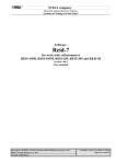
«R2200» multichannel portable device is aimed at registration and analysis of partial discharge distribution in insulation of high voltage equipment.
The presence of the maximum possible hardware and software for pulse noises tuning out
makes the device one of the most effective in the market nowadays.
Figure 1.1.
R2200 outlook
The user can configure the measuring part of the device for the work in real time mode
using the following means:
- the analysis of every pulse waveform;
- the cross matrix for phase to phase comparison, for one measuring channel to another;
- the difference in pulse arrival (the analysis of the «time of arrival» - ToAr), with the
resolution of 2 ns;
- the pulse polarity analysis at several channels simultaneously;
- the inbuilt channels for noise signal control.
The unique feature of «R2200» device which differs it from the products of other firms
is the presence of the inbuilt «PD-Expert» expert system. The «PD-Expert» expert system uses
a set of different means for partial discharge presentation and analysis, including «TF - plane».
There is an inbuilt base of partial discharge images. All the mentioned above gives the opportunity to reveal and differentiate various types of insulation damages and the places they occur.
«R2200» devise should be used by specially trained personnel in scientific centers and laboratories, production shops and in field condition.
3
The devise can be used under the influence of raised electromagnetic fields of power-line
frequency – at distribution substations.
The power supply of the device is universal, which also expands the sphere of its usage. It
could be powered from the supply net or the inbuilt accumulator if high capacity.
The device has metal container housing protecting it from dust and splashes. It has a hermetic membrane keypad.
4
1.2. Technical specifications
The basic technical specifications of the R2200 device are given in table 1.1.
№
Parameter
1 Partial discharge (PD) measuring channels
2 Synchronization channel
3 The time necessary for the whole cycle of all the 9 channel control
4
Frequency range of the registered PD pulse
5
Dynamic range of the registered PD pulse
The phase precision of the definition of the moment of impulse appear6
ance relatively to the sinusoid of power-line frequency
Measurement inaccuracy in definition of the place of PD appearance in
7
cable by means of inbuilt reflectometer*
8 The memory for the storage of the archive of PD measurement in cable
9 The action period of the accumulator
10 Supply voltage of the ac-power adapter
The range of the operating temperatures when working without a thermos11
tat
12 Warranty period of the device and the sensors
13 The device lifetime
14 Dimensions
15 The device weight
Table 1.1.
Value
Up to 9
1
2-30 min
0,5 ÷ 10,0
MHz
70 dB
7,5 degrees
±2 m
256 MB
5 hours
~220 V
-20 ÷ +45
degrees
18 month
not less than
10 years
260х250х80
3,5
Attention!
1) Channel 1 is not isolated from the device container housing.
2) The synchronization channel should be under the voltage in the range of 0.5 up to
48 Volt. For synchronization with the supply net any voltage transformer or AR-1
sensor should be used.
In order to make the data given by the device more precise there is a set of unique diagnostic algorithms for input signal analysis realized in the device.
The most important thing is that all the algorithms work in real time mode,
which makes the insulation condition evaluation on the base of PD level easier.
The basic and the most important algorithms are the following:
- The analysis of frequency characteristics and the waveform* of each input pulse.
- The use of cross matrix for signal comparison that is synchronic comparison of the PD
pulse amplitude in the monitored channel and in other channels.
- The analysis of time delay or advance of PD arrival from the channel under control in
comparison to the impulses coming from other channels. The device is able to differentiate the
PD impulses separated by the length of more than 1 meter of a cable or a bus.
- The analysis and comparison of the polarity of the pulses received from adjacent measuring channels. The specific features of the PD sensors and the schemes of their closed circuit is
that the polarity of the impulse registered in the cable in which the impulse has arisen at, is opposite to the polarity of the impulse in another cable to which this impulse is external.
The use of these algorithms of PD input signals analysis enables to reveal the place of PD
arising in the most precise way, considering the specific features of construction and operation
5
of high voltage equipment of different types. By means of «R2200» the diagnostics of transformers, electric machines, cable lines, switchgears and high-voltage breakers can be carried out.
1.3. The disposition of outer slots
The «R2200» device can be used in two basic regimes – for periodic measurements of PD
level in high-voltage equipment or for continuous monitoring when the device is set at the
equipment for carrying out of stationary measurements. For that purpose the device is provided
with slots which provide operative connection and disconnection of the primary sensors mounted
at the equipment.
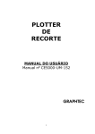
Figure 1.2. The device upper plate
The connection of the cable lines from the measuring sensors to «R2200» device is provided by standard the coaxial BNC slots. At the upper end of the device as it is shown at the picture 1.2 the slots are situated in one row. There are the slots for PD sensors connection, for outer
synchronization connection (Sync), for standard USB cable and net cable connection – for the
work in stationary mode and accumulator charging.
The sensors produced by «Vibro-Center» inc. are isolated from the inner measurement nets
due to their isolating container housing made of ABC with glass fiber addition. The sensors are
connected to the device by means of RG-58U coaxial cables the screens of which are connected
to the body of the sensor and so to the body of the device itself. Therefore the screens of all the
cables are connected to each other but are isolated from the sensors. It helps to minimize the possibility of potential (voltage) presence at the body of the device.
For safety insurance only the sensors supplied with the device should be used together with
the device! If you want to use the sensors of other producers or self-made sensors make sure, that
there is no direct contact between the measurement chains of the sensor (the devise) and the controlled object!
1.4. The R2200 Operation Principles
The R2200 device has 9 input slots for the connection of 9 PD for the registration of electrical PD. All the input channels are equal, independent and have the input resistance of 50 Ohm.
For the means of device reliability each of the input channels has inbuilt protection against incidental pulse noises and the filters which single out DP signals in the range of 1 to 10 MHz.
The operation principle of the R2200 device significantly differs from that of standard oscillographs also used in PD analysis. The basic difference is that R2200 device decides in real
time mode whether the impulse is the result of PD arising in the monitored equipment or whether
it is of other origin. For that special algorithms for input pulse parameters’ evaluation are used.
Thanks to that the user takes part in the analyzing of the impulse distribution only, which optimizes the diagnostics process.
6
The second specific feature of the device is that the impulses of other origin that appear in
the monitored equipment as well as the outer impulses coming along the connection lines are
not taken into consideration by the device. This makes the personnel operation more productive
because there is no need in looking for the place each impulse has arisen at. Finally it lessens the
time of diagnostics caring out and makes the data received more precise.
The device has been designed for PD measurements in different types of high voltage
equipment. The fact that R2200 can be powered by the net and the inbuilt accumulator, small
dimensions and usability make the device well fitting for the use in the laboratory and in the
field.
1.4.1. The description of the basic algorithms of the R2200 input chains
The block-diagram of the input chains of the R2200 device is presented in picture 1.3. The high
frequency input switchboard «Cross point Switches» receives up to 9 signals from the primary
sensors and one test signal from the inbuilt test PD generator. The number of the primary channels is determined by the user in dependence of the specific features of the monitored equipment
and the diagnostic task given. By means of the software operated input switchboard the signals
from the primary sensors in various order can be transmitted to the 9 output channels.
Sensors PD
The Test Generator
signal can be send
Test
Signal
to each of the meaGenerator
Channel
surement channels
by means of the inReference
ner switch board.
Channel
1
Thus the check and
testing of the input
2
Reference
chains is carried out
3
Channel
before each meaCrosspoint
4
surement.
1
Switches
Noise
The registra5
2
tion of the PD sigChannel
6
3
nals incoming from
7
the channels is al1
Noise
ways done sequen8
2
Channel
tially according to
3
9
the user’s choice.
Figure 1.3. Block-diagram of the input chains of the device
The signal from the
channel is sent to
the measurement channel, shown as «Signal Channel» at the block –diagram. Inside the measurement channel the time and amplitude parameters of each impulse are analyzed in real time
mode, and the decision is made whether the incoming impulse is the result of the PD in insulation or whether it is the result of some noise.
The use of the reference channels («Reference Channel» at the block-diagram) play a very
important role in noise resistance. There are a lot of measurement techniques when the validity
of the PD is realized by comparing of the impulse coming from the measurement channel to the
impulse from an additional reference channel. It is a usual practice that the sensor connected to
the reference channel is placed at the object under control and near the basic sensor, or at a certain fixed distance from it. The reference sensor often differs from the basic in inside configuration.
The «Noise Channel» is for realizing the principle of «amplitude sorting out». When an
impulse with the amplitude equal or bigger than that of the impulse of the measurement channel
appear at the noise channel then the impulse blocking the registration of the impulse given ap7
pears at the output of the noise channel. At «synchronous» occurrence on «the noise channel»
the impulse which amplitude is equal or exceeds amplitude of an impulse on «the measuring
channel», on an exit of the noise channel there is an impulse which blocks registration of the impulse.
The specific feature of R2200 devise is that the measurement of DP parameters at every
channel chosen is carried out with the reference to the reference and noise channels. All the
channels work synchronically in real time mode. This is the only way to dejam any noises the
number of which is very high at high voltage equipment.
The user decides by himself the signals of which sensors should be connected to those
“noise” channels. For the channel combination (signal, reference, noise channels) to be chosen
correctly the user should well understand the arrangement of the monitored equipment and the
specific features of the PD impulse arising, spreading and decay in it.
1.4.2. The action of the “sorting out” algorithms for the input signals of the PD sensors
As it was mentioned above the reliability of the high voltage equipment diagnostics depends a lot of the dejam system operation in the device.
It should be understand that tuning out the noises could be done in the most effective way
in real time mode, simultaneously to the measurements being carried out. If the data registered is
analyzed later on, the analysis is much less precise. The fact is that the PD impulses are of high
frequency and the velocity of their spreading inside the equipment is very high. The time gap
between the signals’ of different sensors arriving as small as some nanoseconds could be the
reason for the registered signal screening. All the mentioned above raisers the demands to the
frequency features of the measurement equipment and makes the automatic PD impulse parameter evaluation at registration essential.
A very serious problem connected to the PD impulse recording and “sorting out” is that the
impulse amplitude value often differs as much as in hundreds or even thousand times. Alongside
with that any PD impulse of the smallest amplitude should exceed the amplitude of the measurement device noise. For that the dynamic range of the PD registrator measurement channel
should be not less than 60 ÷ 70 db (the range of the input signal amplitude not less 5000 : 1). Besides the noise level should be low, otherwise the measurement results appear to be much less
precise.
The R2200 device is a modern micro processing unit with a whole set of noise tuning out
functions realized in it. The noise tuning out techniques can be subdivided into three groups:
1 – the simultaneous comparison of the signals received from two sensors of the basic
measurement channel and the reference channel;
2 – the determination of the time gap between the impulses’ coming from the measurement
and the reference channel;
3 – the simultaneous comparison of the amplitude of the impulse coming along the measurement channel and all the other channels.
The first two ways of noise tuning out are realized in the R2200 device thanks to the presence of the «Reference Channel», which determine the reference impulse parameters and compare them to those of the impulse of the PD measurement channel.
The third way of the noise tuning out based on the amplitude comparison is realized in the
R2200 through the use of the «Noise Channel».
1.4.2.1. Let’s look more closely at the PD impulse sorting out technique based on the polarity comparison.
In the device there is a special algorithm of impulse screening out on the base of their polarity comparison with the use of cross matrix controlled by the user. It makes possible to block
the “pulse counting” on the base of the polarity comparison of the impulses coming along the
measurement and the reference channel. The “pulse counting” can be blocked if there is polarity
mismatch between the two impulses. Naturally for such comparison a signal from a PD sensor
(the one according to the user’s choice) should be given to the reference channel. It is important
8
that the sensor is set at the monitored equipment and in correct way. If the signal for the reference channel is chosen incorrectly the effect of this method’s use will be negative.
A
DBT-1
DBT-1
DBT-1
(RFCT-x)
(RFCT-x)
(RFCT-x)
B
C
R2200
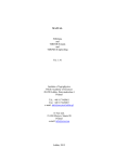
Figure 1.4. The use of the impulse comparison function for the determination of the place of PD arising in transformer or in external
high-voltage equipment
Figure 1.4 illustrates the example of the two impulses’
polarity
comparison algorithm use for the
determination
of
the insulation deterioration in big generators. For that
purpose there are
three sensors set at
the transformer’s
bushings. All the
«DB-2» sensors are
mounted at the test
taps of the bushings.
If the partial
discharge arises in
the basic transformer insulation winding the PD impulse “comes out” through the bushings with
the same sigh. No matter in which direction the impulse goes to, the polarity of the signal outgoing from the «DB-2» sensor will coincide with polarity of the PD impulse, because the bushing is almost ideal coupling capacitor.
If a corona discharge appears at one of the phases if is transferred to the neighboring phases with the other opposite sign.
Thus if the polarity of the signals outgoing from the «DB-2» sensors are opposite we could
say that the PD signal “enters” the transformer, so it is the result of some noises. In case the polarity of the impulses are the same the conclusion can be made that the signals “comes out” of
the transformer, that means that it is the result of the partial discharge which has arisen in the
transformer insulation.
In practice, the cross-matrix is taken experimentally before the PD measurements are carried
\ UA UB UC
out. For that the monitored equipment should be
UA - 82 64
switched off, and the test signals from the generator
– PD imitator are sent to different parts of the
UB 85 - 83
equipment. The amplitude of all the signals outUC 65 84 going the sensors are registered.
An exemplary cross matrix is presented in
Figure 1.5. An exemplary cross matrix
for the PD measurement technique with figure 1.5. The cross matrix has been taken for the
PD measurement in the transformer using tree senthe use of tree sensors in the transforsors. All the tree RFCT-1 sensors are mounted at
mer
the bushings of the HV side of the transformer.
1.4.2.2. The algorithm of noises tuning out on the base of the analysis of the time gap between the arriving of the impulses from different sensors (“time of arrival”) together with the use
of cross matrix is widely used in the monitoring of the spaced equipment, such as electrical generators and motors, cable lines, switchgears.
9
The speed of the electromagnetic wave in the cable lines is a little bit more than half of the
velocity of light. Approximately a PD impulse pusses through one meter of the cable line in 6-7
nanoseconds. It is a very short time but the device is able to control such time gaps thanks to the
use of the modern elemental composition.
Thus we can say that if the distance between two sensors is not less than 1or 2 meters then
it is possible to define the PD pulse direction in the line under control. But it should be kept in
mind that the length of the cables connecting the sensors to the R2200 device should be equal.
Otherwise is the delay in the time of arrival can appear in the cables, which makes the received
data incorrect.
As an illustration of the function of impulse sorting out according to the «time of arrival»,
Figure 1.5. is given. In
the figure an approxCable
imate scheme of PD
Gen
sensors distribution for
the allocation of PD in
generators or external
circuits is presented.
When some PD
CC
CC
signal at the external
terminal of the controlled generator there
always a question apR2200
pears whether the PD
appear inside the generator or are coming
Figure 1.6. The definition of the place of the PD by the method of
from the outside (from
«time of arrival».
the breaker or some
other equipment or even from the input transformer of the plant.
An incorrect answer to the question can lead to significant problems for the high voltage
traffic department. The use of the method of sorting out impulses according to the time of arrival
gives the optimal solvent to the problem.
For example, a generator or an electric motor under control is connected to the supply net
through a short cable by means of high–voltage switchgear. A coupling capacitor in mounted at
each side of the connection cable at each of the phases. The capacitors can be placed in the same
way if a busbar is used in the generator. The minimum distance between the coupling capacitors
(the difference in time of the impulse passing from the PD to the different coupling capacitors) is
1 meter.
If the PD impulse has arisen in the generator then in first will be registered at the coupling
capacitor set at the generator’s terminals. The impulse of the same PD will be registered at the
other end of the cable after a certain time. This delay is the result of the impulse passing along
the cable. For example if the length of the cable is 20 meters the time delay is 6 * 20 = 120 nanoseconds.
For example, if PD appears at the switchgear, then the signal will be first registered at the
capacitor which is situated closer, and in 120 nanoseconds only it will be registered at the coupling capacitor set at the generator.
In the first case the PD impulse is informative for the diagnostic, in the second case it is a
noise and should be excluded from the insulation condition diagnostic procedure.
Here it should be remained once again that the connection cables to all the sensors should
have equal length. It is necessary in order to exclude inaccuracy in the definition of the time of
arrival, as the signal from the sensors also detains in the connection cables. The time of delay is
the same and is 6-7 nanoseconds for one meter of the coaxial cable.
10
1.4.2.3. The algorithm of the noises tuning out by the use of the channel sensibility.
As it was said above this method of noise tuning out is based on the comparison of the amplitudes of the signal coming from the measurement channel and all the rest of the channels.
This method is based on the use of special channels aimed at tuning out on the base of the signal
amplitude, as it is presented on the block-diagram of the input circuits of the device (Figure 1.3).
This way of tuning out the noises is relatively easier than the previous two, as it enables to use
less complicated schemes in the device.
The principle of the impulses’ sorting out on the base of the amplitude comparison is simple. If the amplitude of the signal monitored on the basic measurement channel is less than a
synchronically measured amplitude on any other or a definite channel then the signal doesn’t refer to the controlled object (part of the object). Thus we can say that the impulse is the result of
some PD which has arisen in some other part (of the controlled object) and has induced on the
other put of it.
For the amplitude sorting out algorithm to work correctly it is necessary to pass the signal
to the «Reference Channel» and «Noise Channel». To the output of the channels as much as 1-8
signals can be connected.
Generator
As an example we can say that
the PD current impulse which has
arisen at phase “A”
of the generator, as
it is shown on Figure 1.7., will pass to
the phase winding
CC
“B”
and
“C”
through the internal
R2200
capacitive coupling.
Naturally the amFigure 1.7. Filtering out cross signals by means of the amplitude noise
plitude of the PD
channel.
signal will be less
on “B” phase, and even lesser on phase “C”. So for the method to work correctly it is necessary
to take into account the sensibility of the channels when comparing the signals.
1.4.3. The information presentation in the device.
In the memory of the R2200 device the information on the PD impulses registered in every
channel is presented and stored in the form of amplitude-phase distribution and TF-plane.
Each cell of the amplitude-phase distribution has the following parameters: the phase of
the supply voltage, impulse amplitude, the number of the impulses of the amplitude in the given
phase zone. In the PD impulse distribution matrix one period of the supply voltage sinusoid is
subdivided into 48 zones with the width of 7.5 degrees each (3600 / 48 = 7.50). For the
registration and analysis to be less complicated the impulses with closer amplitudes are taken for
qual. If the amplitudes differ by less than 20 % the impulses are placed in the same cell of the
matrix. The device subdivides the impulses registered into 32 groups according to their
amplitude. The width of every amplitude zone is 2,2 dB. The ratio of the amplitudes of the
maximum and the minimal signals is 5000:1. The general number of the amplitude zones in the
R2200 device is 64 including the zones for the impulses of positive and negative polarity.
11
In each cell of
the PD impulse
tribution
matrix
there is a number in
the range of 0 65535, which is the
number of impulses
of the same parameters, reduced to
one second.
In the Figure
1.9. there is an exFigure 1.8. The example of PD impulses distribution
ample of the PD
impulses distribution in a cable line
of 110 kV. It is evident that the amplitude and the intensity of the PD impulses are maximum
immediately before the supply net voltage becomes maximum. The polarity of the impulses is
opposite to the polarity of the supply voltage. The PD impulse intensity is higher when the
supply voltage passes through 0.
Each cell of
the TF-plane has
the following parameters: the duration
of the impulse first
half-period, the duration of the impulse impulse tinkling sound, the
number of impulses
of the cell.
Figure 1.9. The example of PD impulses distribution.
TF – plate.
Data storage
in the device.
The data registered
can
be
stored in the inter-
nal memory of the device in the form of the distributions.
The measurements stored in the device are structured, the data on each device is stored in a
special directory. The maximum number of the directories stored in the device internal memory
is 32; one directory always exists, as the device never permits to delete the last directory.
1.4.4. The registration of the impulse form and reflect grams.
1.4.4.1. In addition to the registration of the impulse distribution matrix in the device there
is the function of the PD impulse waveform registration, which also enhances the opportunity of
high voltage equipment insulation diagnostics.
As the registration is carried out with very high frequency it is done selectively, during
short periods of time, only when PD impulse is passing. PD impulse registration cannot go on
continuously for a long time. Besides it would demand a lot of working memory the view and
analysis of which would take a lot of time.
The device starts registering the PD impulse form immediately when the leading edge of a
PD impulse comes into the device. The end of the registration of the impulse is defined by the
user and can be chosen in the interval of 2,5 – 80 microseconds.
12
The whole registration period depends of the number of sinusoids chosen. The device internal memory allocated for PD waveform storage can store up to 64 000 reflect grams. After the
registration of all the sinusoids is carried out the user can look through the reflect grams registered.
1.4.4.2. The use of the R2200 device for cable line insulation defects localization.
The method of reflectography is quite widely used in practice for the localization of the
place of insulation defects in cable lines. The method is rather simple and effective, but there are
some shortcomings. The basic are two. First the diagnostics can be carried out off line only. Secondly the defect should be so much developed as to change the wave properties of the cable
line, only in this case the reflection of part of test impulse energy from the defect zone is possible.
The use of R2200 device is also could be used for insulation defects localization, as there
is the module for PD impulse form registration in it. The modified reflectography method used
for it has got some new characteristics in comparison with the standard one. The difference is
that not the impulse of the test generator is used as the test impulse, but a PD impulse arising in
the insulation defect zone.
Figure 1.10 illustrates
the use of PD
Partial
impulses in reflectodischarge
graphy method. In the
Cable
place of the defect in
cable line a PD and as a
result an electromagnetic impulse arises.
Reflectography
From the place of ariby PD pulses
sen the impulse starts
spreading in both the
ways along the cable
line. to trailer cutting of
a cable line. When the
impulse reaches the
Figure 1.10. The use of PD impulses for cable line insulation desensor (in the left part
fect localization.
of the figure) it will be
registered by the R2200
device. On reaching the right end of the cable some part of the impulse energy will be reflected
in the place where the wave resistance has been changed. The reflected impulse with smaller
amplitude will move backwards along the cable. The moment the impulse reaches the left end
of the cable it will be also registered by the R2200 device.
If the registration of the waveform starts the moment the first direct impulse arrives, then
the time chart on the channel will look as it is shown in figure 1.10. For the defect localization
the most interesting is the time gap between the registration of the first direct impulse and the
second (reflected) one. This time has taken the reflected impulse to move from the place of the
arising to the right end of the cable and back to the defect zone. The time of passing from the
defect zone to the left end of the cable takes the same time for both the impulses and so doesn’t
change the time of delay.
In practice the use of the method for defect localization is complicated because of some
reasons.
First the speed of the electromagnetic wave in cable line differs depending on the mark of
the cable. The basic reason of the difference is the difference in the properties of dielectrics and
the constructive difference of cable lines that is the difference in shortening coefficient. Because
13
of that though the time of the second impulse delay is the same, the defect could be situated in
different parts of the cable line.
Secondly a real reflect gram could differ in form from the ideal one, which is presented in
Figure 1.10, as the reflections of the different joints and junction can overlap the “useful” signals
coming from the defect.
Thirdly the measurements of the impulse timing in cable lines under the working voltage is
complicated by the presence of many noises. For the aims of noise rejection the R2200 device
makes a number of measurements (up to some hundreds) and averages the data out. After the
averaging there only the most stable, repeating impulses remain on the time chart.
In the most general case the shortening coefficient is 1.7. If the time of a waveform registration is 80 microseconds, the PD impulse “runs” as much as 14 kilometer along the cable line.
Thus as an impulse “runs” along the cable line twice, so the R2200 device can diagnose a cable
of up to 7 kilometers.
The advantages of the method are the following:
- The possibility the diagnostics of the cable line under the working voltage.
- The revelation of the cable line defects at the very start of their formation.
14
2. General questions of partial discharge measurements
In this part of the manual the general questions of the PD diagnostics as well as the specific
features of PD diagnostic of different types of equipment.
2.1 Partial discharge parameters
Partial discharge is a small spark which appears inside the insulation or on its surface in
high- or middle-voltage equipment. In some time the periodically repeating partial discharges
destroy the insulation which leads to its breakdown in the end. Usually the insulation deterioration can last for month or even years before it fails. Thus the PD registration, localization and the
evaluation of their power and frequency could help to reveal the developing damage and take
measures to prevent the breakdown.
In order to understand the principles of the device operation it is necessary to determine the
basic terms and integrated parameters describing partial discharges in high voltage equipment.
All the standards on partial discharge measurements used in the world define a certain
number of “integral” values which can be calculated or are directly measured while the insulation condition testing is being carried out. The standards of different countries can differ in details but coincide in the basic concepts coincide. In Europe IEC-270 standard is used. The calculated parameters in the R2200 device go by the American standard, as the device has been developed for the joint sales in the Russian and American markets. In Russia its own standard on partial discharge is being developed, but it has not been finished yet.
All PD standards are based on the concept of "pseudo glow discharge". The "pseudo glow
discharge" is the discharge which should be instantly “injected” into the monitored equipment in
order to regain the balance which has been disturbed by the PD impulse. The basic thing in the
definition is that we do not know the real parameters of a partial discharge which arises for example inside the gas occlusion, but measure the reaction of the monitored high-voltage equipment in the partial discharge appearance. The discharge is called “pseudo glow” because we can
only suppose its presence but we do not know its real value. The pseudo glow PD is measured in
pC (picocoulomb). If we summaries all the discharges which has been registered in the equipment in one second it will be the PD current - the current that passes through the circuit controlled by the sensor additionally, as the result of PD arisen.
Historically important is such characteristic as “maximum measured discharge”. Almost all
the high-voltage equipment producers use this value (if any at all) at the commissioning tests. It
is evident that something statistically reliable should be measured. In old devices the statistic is
based on average timing, but in modern ones the problem is decided by excluding from consideration single casual impulses. For example in the definition of the American standard it runs as
follows: "amplitude of the greatest repeating category at supervision of constant categories".
Consequently the term does not include the analysis of single impulses. For the definition to be
more precise let’s take into consideration the partial discharges which repeat as often as 10 times
a second. In this case if the supply net frequency is 50 Hz one impulse should appear not less
than one in 5 periods of the net. For the convenience of the use we’ll define the term as follows:
a PD impulse will be considered to be periodically repeating if it urns as often as 0,2 pulse for
one period of the supply network. Further on in the text the parameter will be indicated as Q02, in
the same way for 50 and 60 Hz.
The value of the parameter is quite high. There are a lot of methods based on it, though
when used separately it is not so reliable, at least for the continues monitoring under the working
voltage. There are lots of equipment where partial discharges of big amplitude are registered and
the equipment runs for years but PD of small amplitude but repeating often indicate a real problem.
15
How to count the losses caused PD? It is quite easy to do physically. At every PD impulse
we additionally inject a pseudo glow discharge from the source of testing voltage into the controlled object. The discharge is injected instantly and depends on the voltage of the supply net.
So the energy that additionally enters the equipment because of the single PD is equal to the
charge multiplied by the instantaneous voltage in the object. By summing up all the impulses we
can get the full PD energy. If we divide the full energy by the whole time of summing up we’ll
get the PD power. The parameter is called “energy loss for partial discharge”.
Formula:
1 m
P
Qi Vi
T 1
where:
P – discharge power, W,
T – time of monitoring, sec,
m – the number of impulses registered during the time T, and
QiVi – the energy of the I impulse
Evidently that on the base of the PD impulse phase distribution it is possible to calculate
instantaneous value of applied voltage, in case the phase bunding of impulses is done correctly
and the power is calculated in the right way. But not all the devises can register impulse phase
distribution, and if the function is realized the sensor can register impulses from two or even
three phases of the object. So it is difficult to understand what voltage from what phase should
be taken into account. In order to solve the question the American standard uses one more diagnostic parameter - PDI - "Partial Discharge Intensity". In this parameter the effective value of
the voltage is taken instead of instantaneous voltage of the moment of a PD passing, that is the
voltage equal for all the impulses but not the personal for each of the impulses. If we compare
the results of the calculation in both the cases we can see that they differ in the range of 20 %. It
is quite enough to estimate the level of PDI correctly and to build a trend. PDI parameter is one
of the basic parameters used for the evaluation of the PD intensity in the controlled object.
2.2. Input Circuits Calibration
One of the important problems that needs to be solved when using the PD control devises
in practice is the problem of the devise calibration.
It is necessary to understand that unlike the measurements of the standard parameters of
electric circuits, such as currents, voltages, a PD measurement devise cannot be calibrated and
adjusted neither at the place of production nor by any metrological service.
The reason is that, as it was mentioned above, those are not the PD parameters that are
measured but the secondary characteristics of the of the partial discharge that is the reaction of
the controlled object on the potential redistribution. Thus one and the same partial discharge in
insulation will be measured by our devise in different ways at different objects. For example an
impulse of 100 pC arising inside different equipment will induce in one and the same sensor a
signal differing in amplitude in tens or even hundred times. It will be so at PD measuring in a
transformer or a small electrical machine. Thus in the second case the PD impulse signal will be
much more.
The real sensitivity of the device, which is the potential metrological parameter, influencing the parameters being measured, is not a constant. It depends much of the conditions under
which the measurements are carried out.
The sensitivity of the device depends on:
- the type and the mark of the controlled high-voltage equipment, as well as transformers,
generators and cable lines;
- the type and the disposition of the PD measurement sensor;
16
- the insulation defect localization: the impulses arising on various distance from the sensor
will induce on the sensor the signals of different amplitude in the sensor;
- the connection cable length etc.
You could never allow for all the perturbing factors which influence the measurement
scheme sensitivity beforehand. It is evident that the only possible way to get the reliable data by
PD measurements in high-voltage equipment is to calibrate the measurement scheme right onsite. Any change of the measurement scheme parameter, or the sensors’ localization, etc. demands recalibration of the measurement scheme.
The calibration procedure preceding PD measurements includes the following:
- An individual measurement scheme is assembled at the switched-off high-voltage equipment need to be monitored
- Artificial partial discharges with the amplitude known are injected into the zone of the
object which is planned for monitoring
- The output signals from all the sensors mounted at the equipment are measured
- Starting from the known level of the test impulse, injected into the equipment, the real
sensitivity index is calculated for each of the measurement channels of the measurement scheme.
- The calculated indexes of the channel sensitivity are used in all the further PD measurements carried out under the working voltage or testing voltage.
It is evident that the only way to make the PD measurements reliable is to include test generator into the measurement complex. The generator should produce impulses corresponding to
the PD impulses. The generator should be rather compact and have accumulator power supply.
Thus all the PD measurement equipment produced by Vibro-Center Ltd. include GKI-2
generator, imitating PD impulses. Thanks to that the users can calibrate the measurement
schemes by themselves at the laboratories and in the field condition.
2.2.1. GKI-2 Impulse Generator
The GKI-2 is intended for PD registration circuits calibration before carrying out
the measurements. It can be used at the laboratory and in the field condition. It can work at
the ambient temperature of up to 20 degrees
below zero.
The device is run with the help of membrane keyboard; all the information is disFigure 2.1. GKI-2 Generator
played at the LCD display.
The generator is powered by two «АА»
batteries, or an accumulator of the same size. One charge of the accumulator is enough for the
generator to work during not less than 10 hours. A charger is also available with the generator, to
feed the generator during the work.
The GKI-2 generator usually injects the charge of 3000 pC into the controlled objects and
the measurement circuits. It gives the opportunity to calibrate measurement circuits before carrying out the measurements in consideration of signal decay in the object. We also produce the generator with the function of injected charge control. In this case the user can choose the injected
charge value in the range of 2000 - 5000 pC.
At the front plate of the devise there are the display and the membrane keyboard. At the
upper left corner there is the name of the device; in the upper right corner there is the VibroCenter emblem.
The keyboard outlook is presented in the Figure 2.2. For the device operation four functional keys are used.
Keys’ function:
"On" – the key for the device switching
On
Set
on/off.
"☼" - display illumination switching on/off.
Figure 2.2.
17
"Set" – the key for stopping the generator and switching over to setting the operation
modes.
"Mod" – the key for choosing the mode of operation.
The device slot is meant for connection of the measurement circuit with the standard resistance of 50 ohm. In case such load resistance is absent the device readings are invalid.
There are two working mode in the device:
- autonomous impulse generation;
- the device parameter setting.
The device switches on at pressing "On" key. After the power supply is applied to the device, after testing and software loading the device switches over to the mode of autonomous impulse generation according to the parameters set during the previous session.
The generator produce impulses of 3000 pC (at 50 ohm) with the frequency of 24 kHz.
Changing the current generator parameters are done in the setting mode. The setting mode
is available at pressing "Set" key. Each pressing of "Set" key results in changing of the current
setting parameter. At the last "Set" pressing the device switches over to the mode of registration.
All in all three parameters are available for setting.
The user can set:
- The operation period before automatic switching off after the last key pressing. The user
can choose the period to be 1, 10, 20 or 60 min, or the mode can be switched off. The following
notice will be displayed: "Switch off Device – 10 min". The function is aimed at the battery saving.
- The time of display illumination. It could be 1, 5 or 10 min. The notice "Switch off light.
– 1 min" will be displayed. The illumination is necessary when generator setting is being carried
out, but in the process of impulse injecting when the user is working with the device there is no
need in it.
- The display contrast. It can be changed from 0 to 100% with the step of 10%. The notice
"CONTRAST – 20 %" is displayed.
In the upper right corner the level of the battery charge is schematically displayed. Each
line of the schematic battery indicate 20 % of the charge. In the main field of the display the
magnitude of the charge injected into the outer circuit is displayed (3000 pC).
In the bottom of the display the time left before the generator automatic switch off is
shown in the form of a moving line. The time is indicated at the slider in arbitrary units of the
maximum value set by the user. If the function is switched off the slider does not move. To the
left of the moving line the remaining time is presented in digital form.
Figure 2.3. The form of the generator outgoing impulse registered
by oscillograph
The form of the
test impulse from the
GKI-2 is presented
in figure 2.3. The duration of the leading
edge of the pulse is
approximately 5ns.
The trailing edge of
pulse is of more duration, but it does not
so much matter for
the scheme calibration procedure. Real
PD impulses are often
of the same form.
The
output
cuit of the generator
18
should always be loaded so that the resistance would not exceed 50 ohm. The short-circuit condition of the output circuit of the generator is not dangerous for the workability of the device. It
can stay in the condition any time long and continue to inject into the object the PD impulses of
the amplitude indicated at its display.
If the monitored object concerning points of connection of the generator, has resistances
much exceeding 50 ohm, the form of the test generator impulse gets distorted. The wave properties of the monitored object change and the calibration procedure will be incorrect.
In order to exclude the possibility it is necessary to connect the “terminator” with the resistance of 50 ohm, available with the generator, in parallel with the monitored object. For that purpose a standard «T-Connector», also available with the generator, is connected to the generator’s output. Loading “terminator” is connected to one side of the «T-Connector». To the second
side the cable is connected for the impulses to pass to the calibrated object. As a result the form
and the amplitude of the test impulse will have standard parameters.
2.2.5 Channel Sensitivity Calculation
The calculation of sensitivity device channel can be made automatically by means of the
built in the R2200 device function "calibration" described in point 3.3.4 of the given instruction,
or in a manual mode.
For manual calculation of the sensitivity factor, after registration of measurement with the
injected charge from the generator, it is necessary to define signal level (MV) which has been
registered by the device on the calibrated channel. It is possible in the device by means of the
measurement viewing, or after downloading of the data of the calibrating measurement into the
computer and analyzing it by means of the "IHM" program, available with the device.
The sensitivity factors are calculated in the following way. It is necessary to load the measurement from device archive into the computer, and look at the signal level (Q02) on the calibrated channel.
At the use of "IHM" software the signal level can be defined at graphic viewing of data in
MV scale.
Further sensitivity of each measuring channel of the device can be calculated easily under
the simple formula:
Qgenerator
CCS
U InputChannel
Where:
CCS - The factor of sensitivity of the measuring channel, for the given partial discharge
measurement scheme is calculated in (no/V);
Qgenerator - the impulse amplitude at the output of the calibrating generator measured in
“Nan coulomb” (no) read out from the generator display, or controlled by an oscillograph;
U InputChannel - the voltage amplitude from the sensor, measured at the measurement channel
input, measured in “volt” (V).
Example. After injecting into the monitored object a test impulse with the amplitude of 3
nC, there was an impulse with the amplitude of 300 mill volts or 0,3 volts registered at the input
of the device measurement channel. So the total calculated sensitivity of the measuring channel
of the device, in the given measuring scheme, is equal to 10 "nanoCoulomb/volt" (nC/V).
Attention: the sensitivity is entered into the device in Nan coulomb/volt, therefore there is
3 nC in the formula, injected by the generator and the signal level is reduced to Volts.
19
3. How to work with the R2200 device
The "R2200" device is incased into the metal case, has liquid crystal color screen with the
resolution 640x480 points and the keyboard blind in the case. Management of device functions is
carried out by means of the keyboard. At the keyboard there are cursor command keys "▲",
"▼", "◄", "►", enter - "Ent", cancel - "Esc", "Mem", "Shift", "Help" functional keys "F1" "F5", keys of switching the device on/off " ".
3.1. The Main Functions for the Information Loading and Editing
3.1.1. The use of the functional keys
In windows of adjustment, archive viewing or measurements the bottom part of the screen
is divided into five parts on which buttons are drawn, and the short help about the action made
by pressing to corresponding button of a function key is written.
3.1.2. Choosing of the parameter for editing
In order to change a parameter in the windows of the device adjustment you should move
the cursor to the necessary parameter (the arrow to the right " ") by means of keys "▲" and
"▼".
3.1.3. The value entering
For value editing press "Ent" key at the corresponding parameter. If the values of the numeric parameter are fixed (such values are underlined, after entering function is activated)
choose the value by "▲" and "▼" keys. In all the other cases you can move along the input line
using "◄" and "►" keys, and change the value of the parameter by "▲" and "▼" by cyclic
search (from 0 to 9). In the input line press "Ent" to finish the entrance and "Esc" for cancelling
– in this case the value will not change.
3.1.4. Text entering
For text editing press "Ent" key at the corresponding line. The window for text entering
will appear.
Figure 3.1. Text entering window
Use "◄" and "►" keys to move along input line; use "▲" and "▼" to choose the parameter value by cyclical search.
If you press "Shift" or "F1" in the name input window the keyboard window will appear
for quick text entering.
20
Figure 3.2. The keyboard for quick text entry
In this window:
The cursor control keys "◄", "►", "▲", "▼" change the character in the input
window;
"Ent" – replaces the edited character in the input line by the chosen in the window
with moving to the next character editing;
"F1" – deletes the current character in the input line and shift the line;
"F2" – deletes the previous character in the line and shifts the line;
"F3" – replaces the current character of the input line by “space”;
"Shift+Left" and "Shift+Right" - does cyclical shift to the editing of the next character in the input line;
"F5" – shifting from English to Russian;
"Esc" – closes the window of the quick entering and shifts to the mode of standard
line entering.
In the input line press "Ent" for input finishing or "Esc" for cancelling – in this case the
value of the line will not change
3.1.5. Choosing the value
The parameters marked with
change by pressing cursor control keys "◄" and "►".
3.2. Switching On the Device
At switching on the device (by pressing "
" key) the visit card window will be displayed:
Figure 3.3. The "R2200" visit card window
21
In the given window the information on firm-manufacturer and the software version is displayed. Simultaneously with switching on the device its testing begins. After testing is finished
the device loads up the data of the last measurement and shifts to standby mode waiting for the
commands from the user and communication interfaces – it is the basic operating mode of the
device.
The user commands to the device by means of pressing of the keyboard keys using the device menu. For entering the device menu press any key except " ".
3.3. The R2200 Device Function Setting by Means of the Inbuilt Menu
The main menu of the device is presenter at the picture:
Figure 3.4. The "R2200" device menu
At the upper left corner of the display the level of the battery charge, the current date and
time are represented.
In the main - central – part of the display the name of the chosen menu and the icons of
the enclosed points are represented.
Shifting from point to point is done by pressing "◄" and "►" keys; choosing of this or
that point – by "Ent" key, choice cancellation – by "Esc". At shifting form point to point by "◄"
and "►" keys, the cursor arrow (
) also moves, specifying the point which will be chosen by
pressing "Ent.
By pressing functional keys "F1" - "F5" the point of the menu corresponding to the icon
located over the key will be chosen.
Structurally the device menu looks as follows:
"ЧР registration" – the menu of PD measurement starting (see point 3.3.1);
"Reflectometer" – calls out PD oscillograph (see point 3.3.2);
"Setting measurement parameters":
o "Channel parameters" – setting measurement parameters different for every
channel (disassembling, sensitivity) (see point 3.3.3);
22
o "General registration parameters" – setting measurement parameters general
for all the channels (the type of synchronization, the number of sinusoids)
(see point 3.3.4);
o "The device calibration" – the calibration of the PD measurement circuits
(see point 3.3.5);
"Working with the archive":
o " Working with the data archive " – directory creating and deleting , measurement view and deleting (see point 3.3.6);
o "Setting the parameters on default” – changing the parameters to default
values with archive cleaning (see point 3.3.7);
o "Renewing wearing" – program loading into the device.
"General settings of the device" - the time parameters of the device: the time and
date specification, the time of the device switching-off, the time of the display illumination switching off (see point 3.3.8);
3.3.1. Measurement menu
The device can carry out the full measurement or the measurement on one of the channels
chosen. The full measurement is carried out on all the switched on channels in accordance with
their settings. The measurement on a single channel is carried out on the channel chosen, no matter whether it is switched on or not.
For entering the measurement menu choose the first point ("F1") in the general menu of the
device. The window will appear as it is shown in figure 3.5.
Figure 3.5. Measurement menu
The device is ready for carrying out the full measurement. For starting measurement on a
single channel, point to the line “single ch.#” by the cursor arrow, using "▲", "▼" keys. By "◄"
and "►" choose the necessary channel (for details see Information Input). Returning to the full
measurement is done by "▲" and"▼" keys.
The following functional keys are available at this window (see point 3.1.1).
o "F1" – «Start» measurement starting, you can also press "Ent" key;
23
o "F2" – «Param.» setting measurement parameters, different for each channel
(disassembling, sensitivity, see point 3.3.2);
o "F3" – «General» setting the measurement parameters, general for all the
channels (the number of sinusoids, the synchronization type) (see point
3.3.3);
o "F5" – «Cancel» exiting the measurement menu; "Esc" key is also available.
After starting up, the device carries out the calibration and starts the data reading, displaying the course of measurement with the states bar.
Figure 3.6. Measurement
For cancelling the reading press "Esc". Cancelling the measurement on the given channel
you will not loose the previously read data (on the previous channels of the device). After the
registration the saved measurement is displayed (see point 3.3.8).
3.3.2. Reflectometer
The window of partial discharge oscillograph, working with inbuilt reflect meter is called
out.
24
Figure 3.7. Reflect meter parameters
The algorithm of the reflect meter work is the following: after a partial discharge comes to
the input, the signal registration begins with the interval of 10 nanoseconds, and lasts for the period chosen. There could be registered up to 64 thousands of such signals. The whole time of
registration depends on the chosen number of sinusoids of the supply net.
For cable analysis there is the function of oscillograph in the R2200 device, which is the
registration and viewing of all the intervals, without averaging.
After choosing the menu point the Reflectometer parameters window will be displayed.
Choosing of the parameter is done by "▲"and "▼"keys. For details see point 3.1.3 and 3.1.5.
In the window that has appeared you can specify the following:
1. The registration channel
2. The number of sinusoid periods
3. The length of the monitored cable line for excluding knowingly false results.
4. Shortening coefficient. If there is the opportunity define the PD spreading velocity in the
cable. It can be calculated with the help of PD generator, if the gap between the impulse
and its reflection is known (for example to the joint or to the end of the cable line).
5. Choosing starting up mode. The starting up mode is necessary for defining of the amplitude threshold and the impulse registration phase windows.
6. The threshold of the reflectometer starting – the impulses surpassing the threshold will
be registered.
7. Gain coefficient
8. Choose the synchronization time and the phase of the power supply voltage.
At free starting up there is the parameter available The reflect meter starting threshold in
mV – that is the starting point of registration. At other starting modes the threshold is chosen in
agreement with the registration zone chosen.
For the reflectogram registration in a definite amplitude-phase window it is necessary to
choose the starting mode.
It is possible to set the amplitude-phase windows after PD measurement on the given
channel so that there was no situation when an attempt is made to register the "oscillogram" of a
PD which are not present. For this purpose it is necessary to establish the «After registration»
starting mode and to press «F1» key - "Next", PD registration will be made. After the registration
the AF - distribution of the registered impulses- will appear in the screen.
25
It is also possible to choose the amplitude- phase windows in the previously registered
measurement, choosing it from the measurement tree. For that choose the registration mode
«Measurement selection» and press «F1» key - «Next». When the tree of measurements will appear, choose the necessary measurement and press «Select». The AF - distribution of the registered impulses - will appear in the screen.
Figure 3.8. Measurement selection
It is also possible to choose a zone in an empty measurement. For that choose the «Zone
selection» starting mode. There will the AF-distribution window appear in the screen, but as the
measurement has not been carried out the window will be empty.
Figure 3.9. Zone selection
In this window you can choose the zone by the 3 cursors. Red and green cursor chooses
scopes of phase for pulses registration. Blue cursor chooses amplitude scope. Search of cursors is
made by “F2”, color square with the color of present cursor is for prompting. Cursors for phase
choosing are moved from 0 to 180 degrees. Registration will be made symmetrically relatively
180 degrees. Active zones for registration are marked by blue color for positive and negative.
The example of zone choosing is on the figure 3.10.
26
Figure 3.10. Zone selecting
After zone selection press «F1» - «Start» for starting reflectogram registration. At the
first registration the device calibration is carried out; for the further registrations the previously
received calibration coefficients are used. The processing of the data registered takes some time
which is indicated by a the corresponding message on the screen. After that the window for the
reflectogam viewing will be displayed (see point 3.3.10 Reflectogram viewing).
The following messages appear if there is an error in the oscillograph operation:
(1)
- "Synchronization error!" – the measurement cannot be registered as the device
could not define the synchronization frequency. Make sure that the synchronization channel is connected and try again.
(2)
– "The signal amplitude surpasses the registration borders". The error can appear
if gain coefficient is too big. When the error occur the automatic decreasing of
the given coefficient will be suggested, till the registration amplitude is optimal
for registration. For the press «Enter»; at pressing «Esc» the measurement will be
displayed in the form it has been registered.
(3)
– "The impulse limit is surpassed!" The error can appear if the PD impulses come
too quickly and the device is unable to register them, especially if the cable is rather long. It often happens if the registration is carried out at the noise level; as a
remedy you should turn up the reflectogram registration threshold. If the error
appears the device automatically suggests to turn up the threshold; then the reflectogram will be made with the new parameters.
(4)
- "The maximum threshold for the given gain coefficient has been achieved" If
this error occurs reduce the gain coefficient.
3.3.3. Channel parameters
For specifying the measurement registration parameter choose point 2 – "Measuring
scheme configuration" in the main menu of the device. For specifying the channel parameters
choose the first point - "Channel parameters".
27
Figure 3.11. Channel parameters
Reading of the data from the device channels is done sequentially, the input channels are
one by one connected to the measurement channel. The rest 8 channels at this time can be used
for noise rejection with the help of two reference and two noise channels. In this window you
can specify the signals from which channels will be read and where will the rest of the channels
be connected to.
For the measurement scheme editing to be more convenient you can use functional keys.
"F1" – «Template» - selecting one of the ready measurement schemes. (see point 3.3.3.8.)
"F2" – «Copy» - copying the channel parameters (see point 3.3.3.9.)
"F3" – «Common» at pressing the key the window with the general registration parameters
will appear (for details see General registration parameters).
"F4" – «Save» - saving the changes of the configuration.
"F5" – «Exit» - exit without saving. For exiting without saving you can also press "Esc"
key.
The «Measurement scheme configuration» window can be subdivided into the following
levels:
The level of registration channel selection (see point 3.3.3.1.)
The level of synchronization type selection (see point 3.3.3.6.)
The level of angle input
The level of the basic (measurement) channel I (see point 3.3.3.2.)
The level of the reference channels II, III (see point 3.3.3.3.)
The level of the noise channels IV,V (see point 3.3.3.4.)
The level of cross matrix (see point 3.3.3.5.)
The level of the plant name input (see point 3.3.3.7.)
The level of the object name input
The level of the scheme name input
At first the level of channel registration selection is active (see Fig. 3.12.). For shifting between the levels use "▲" and "▼" keys.
3.3.3.1. Registration channel selection
For channel registration selection it is necessary to shift to the level of «registration channel selection» and to select the channel with the "◄", "►" keys. You can rundown the channels
28
from any other level by pressing the combination of keys "Shift+◄", "Shift+►". The number of
the active channel will be marked by color. The channels excluded from the registration are displayed in pail color (see Figure 3.12.).
Figure 3.12. The registration channel selection level
3.3.3.2. The input of the main (measuring) channel I parameters
The channel chosen at the level of “registration channel selection” is automatically connected to the main (measuring) channel. The short information of the current parameters of the
channel is displayed: the power net voltage phase, sensor type, channel sensitivity (see Fig.
3.13.).
The channel chosen at level is automatically connected to the basic (measuring) channel of
"a choice of channels of registration». The brief information on current parameters of this channel is deduced also: a phase of pressure of a network, gauge type, sensitivity of the channel (see
Fig. 3.13 ).
29
Figure 3.13. The level of the main (measuring) channel I
You can enter the level of the «measuring channel» with "▲" and "▼" keys or pressing
"Ent" at the level of «channel registration selection». For the measuring channel parameter editing press "Ent" – the pop-up menu of measurement channel parameter editing will be displayed.
(see Fig. 3.14.).
Figure 3.14. The measurement channel parameter editing menu
In this menu it is possible to change the following parameters: switching on/off the registration channel, channel sensitivity (no/V) (the channel sensitivity is specified during the device
calibration and influences the amplitude form mV to pick, and PDI calculation; the sinusoid shift
regarding the sincroimpuls – on how many degrees the matrixes should be shifted on all the
channels of the device. At display of matrixes of PD distribution the device will shift the PD ma30
trix on each of the channels by the value specified at this point and add to the shift for every
channel the value specified during the channel tuning (Figure 3.12). А value – corresponds to 0º,
B – 120º, C – 240º, AB - 60º, BC - 180º, CA - 300º. The shift is done during the displaying, the
matrix remain unchanged. Thus if at the moment of registration the shift has been specified incorrectly you can make the data look correct by changing the value to the correct one.
Shifting from point to point of the menu is done with "▲" and "▼", selecting of the value
is done by "Ent" and "◄", "►", depending of the parameter (for details see point. 3.1). For the
data saving press "Mem" or "F4", for cancelling press "Esc".
3.3.3.3. Entering the parameters of the reference channels II and III
For choosing the necessary reference channel move to the “reference channel” level with
"▲" and "▼" keys. Shifting between the reference channels is done with "◄"and "►" keys. For
each reference channel the number of the channel connected to it is displayed («#» means that no
channel is connected that is the filter is switched off), as well as the short information of the
channel parameters: the filters switched on and the shift regarding to the measurement channel,
in % (see Figure 3.15.).
Figure 3.15. Reference channel level
For the reference channel parameter editing press "Ent" - the pop-up window of the reference channel parameter editing will appear (see Figure 3.16.).
31
Figure 3.16. The menu of the reference channel parameter editing
In this menu you can do the following: choose the number of the channel connected to the
reference channel of disconnect a channel by choosing «#»; switch on/of the polarity filter,
switch on/off tuning on the amplitude; shift with respect of the measurement channel in % (the
necessary parameter when tuning on the amplitude is switched on), switch on/off the time of arrival filter and specify the and also define the condition of signal blocking in case the time of arrival filter in switched on (by advance or by delay). Shifting from point to point is done by "▲"
and "▼"keys, selecting the point by "Ent" and "◄", "►", depending on the parameter (for detail
see point. 3.1). For the parameter saving press "Mem" or "F4", for deleting "Esc". Attention! If a
channel is chosen at least one of the filters should be switched on, otherwise the data will be considered illegal and the corresponding worming will be displayed (see Fig. 3.17.).
32
Figure 3.17. Illegal data entering
3.3.3.4. Entering the noise channels IV and V parameters
For the noise channel selection move to the noise channel level by pressing "▲" and "▼".
Shifting between the noise channels is done with "◄" and "►"keys. To every noise channel up
to three channels can be connected, the numbers of the channels are displayed at the channel
screen («#» symbol means that no channel has been connected). Short information on the current
parameters of the channel is also displayed, such as whether the tuning on the amplitude is
switched on (tuning on the amplitude automatically switches on in case at least one of the channels has been chosen on the noise channel given) and whether the shift in respect of the measurement channel in % is switched on (see Figure 3.18.).
Figure 3.18. Noise channel level
33
For noise channel parameter editing press "Ent" – the pop-up menu of noise channel editing will be displayed (see Figure 3.19.).
Figure 3.19. Noise channel parameter editing menu
In this menu you can change the following parameters: choose the numbers of three channels connected to the noise channel or disconnect by pressing «#», choose the shift in respect of
the measurement channel in %. Shifting from point to point is done by "▲" and "▼"keys, selecting the point by "Ent" and "◄", "►", depending on the parameter (for detail see point. 3.1). For
the parameter saving press "Mem" or "F4", for deleting "Esc".
3.3.3.5. Viewing and editing of the cross-matrixes and the channels’ sensitivities
The channel sensitivity (nC/V) is defined at the device calibration, and influences the amplitude conversion from mV into pC, as well as PDI calculation. Cross talks from channel to
channel in % are also defined during the calibration and influence the registration if the noise
rejection on the polarity basis is switched on.
For cross-matrix editing move to the necessary level with "▲" and "▼" and press "Ent"
(see Fig. 3.20.).
34
Figure 3.20. Cross matrix level
The table with cross talks and channel sensitivities will be displayed (see Figure 3.21.).
Figure 3.21. Cross matrix
Moving through the table is done with "▲", "▼", "◄", and «►". In the table the crass
talks (necessary for the registration in case the polarity filters are switched on) in dependence of
the measuring scheme are marked with dark-blue; the rest if the cells are light blue. In the horizontal line the numbers of the registration channels are listed. The channels which are off the
registration are marked in pail color. The active element is marked out with inversion, for editing
press "Ent" (for detail see point. 3.1.3). For quick editing of the table use functional keys.
"F1" – «All, sens.» the sensitivities of all the channels are the same as that of the active
element (for that you should be in the corresponding cell). Before the measurement is carried
out the warning for the action confirmation will be displayed (see Fig. 3.22).
35
Figure 3.22. Changing all the channels’ sensitivities
"F2" – «All, matrix» - copying the values in the table like that of the active element. At
pressing the key the pop-up menu will appear and you can choose what part of the table should
be filled with the value chosen: the line, the column or the whole of the table. The selection is
done with "▲" and "▼" and "Ent". Before the changes are inserted into the table the pop-up
warning for the action confirmation will be displayed (see figure 3.23.).
Figure 3.23. Quick editing of the cross-matrix
"F3" – «Clear» - setting the values on default. For specifying the sensitivities on default
(the default value is 10 nC/V), the sensitivity cell should be active. For specifying the cross talks
on default (the default value is 100%) the matrix cell should be active. Before the changes are
36
carried out the message for the action confirmation will be displayed (see Figure 3.22., Picture.
3.23.).
"F4"- «Save» - saving the changes entered into the configuration.
"F5"- «Exit» - leaving without saving. For leaving without saving you can also use "Esc"
key.
3.3.3.6. Selecting of the synchronization type
For choosing the synchronization type move to the corresponding level using "▲" and
"▼", then press "Ent". The following pop-up menu will be displayed (see Figure 3.24.).
Figure 3.24. Choosing synchronization type
The synchronization types available:
o External – when PD is being measured the device is synchronized according
to the external input "Sync";
o Channel 1 – when PD is being measured the device is synchronized according to the external input 1;
o No sync. – the device is synchronized according to the inbuilt timer working with the chosen frequency (50 or 60 Hz);
Selecting is done by pressing "▲" and "▼" and "Ent" or "Mem"; for cancelling press
"Esc". When external synchronization is chosen the level of the angle entering becomes active.
For its entering move to the corresponding level by pressing "▲" and "▼" and press "Ent", and
you will get the opportunity of the value entering (for detail see point 3.1.3).
3.3.3.7. Entering the name of the plant, object, scheme
For entering the name of the plant, object, scheme move to the corresponding level by
pressing "▲" and "▼" and press "Ent". The pop-up menu will appear for entering the text (for
detail see point 3.1.4.).
3.3.3.8. Working with the ready templates of the registration schemes
You can store the ready templates of the measurement schemes. For working with the templates press "F1" - "Template" in the window "Measurement scheme tuning".
The pop-up window will appear:
37
- Create template. Before template creating fill in the blank fields in the current configuration. At choosing the point of the menu the window for template name entering will appear; at
pressing "Ent" the current configuration will be saved in this template and the template will be
included into the list of templates.
- Load template. The list of the templates available will be displayed. "F1" – viewing of the
current template, "F2" – deleting the template from the list, "F4" – selection – that is loading the
template in the current configuration; "Exit" – exiting from the current window.
Figure 3.25. Working with templates
3.3.3.9. Channel parameter copying
For quick editing of the channel parameters you can copy the parameters from the channel
chosen to the other channels. For that press «F2» - «Copy» in the window «Measurement
scheme tuning».
38
Figure 3.26. Channel parameter copying
For choosing the channel you want to copy the parameter from place the cursor opposite
the line «Channel’s parameters:» and set the number of the channel you need with "◄", "►"
keys.
For excluding a parameter from copying delete the check mark in the corresponding field.
You can choose the necessary parameter with "▲", "▼", set/delete the check mark with - "Ent".
In this window the following functional keys are available:
«F1» - «All params.» - at choosing the function all the channel parameters are checkmarked, so all the parameters will be copied to the other channels.
«F2» - «All channels» - at choosing the function all the channels will be check marked,
thus the chosen parameters could be copied to all the channels.
«F3» - «Copy» - at choosing the function the chosen parameters will be copied to all the
channels.
«F4» - «Save» saving the changes in the current device configuration and returning to the
previous window.
«F5» - «Exit» returning to the previous window without saving.
3.3.4. Common registration parameters
For setting the common parameters of measurement registration select point 2 “Measurement parameter setting” in the main menu of the device. For setting the channel parameters select point 2 “Common registration parameters” (see Figure 3.27.).
39
Figure 3.27. Selecting the point «Common registration parameters»
The window with common registration parameters will appear.
Figure 3.28. Common registration parameters
Here you should define:
- Working voltage, in kilovolts, influences the impulse intensity PDI;
- Level, to which it is necessary to count PDI (middle of amplitude window in mV is imaged in the informational field for exclusion noises from account PDI meaning. Windows
after that isn’t in the account). Detection of noise level is switching automatically if level
meaning is “auto”;
- Maximal duration of PD and pause after it;
- Quantity of sinusoid periods – averaging for PD measurements (stated quantity of net period will be registered for every amplitude window). Quantity of pulses will be up to 1 second
after registration.
- To make type of timetable for signal registration. Registration of signals can be made in
the manual mode in the menu – “launch of registration” and by the timetable. You have a possibility to place 50 time meanings for registration when you choose type of timetable “by the
time”. If you choose type of timetable “interval”, you have a possibility to place interval meaning, through which signals registration will be made. If you need to switching loss registration by
the timetable or type “never”.
40
3.3.5. Device calibration.
It is necessary to make calibration for correct count PDI, correct detection of pulses amplitude in used units (pC) and also for correct scrapping pulses in the switching on filters by the polarity before measurements on every object. You need to choose in the main menu of device
point 2 – “Installations of measurements” and then point 3 – “Calibration of device”.
Figure 3.29. Calibration of device
In this window:
- to install amplitude of injected pulses by your generator (in nC for GKI-2 amplitude is
3,0 nC – this is meaning on default), press key "▼";
- to install frequency of pulses which are injected by your generator (in kHz for GKI-2 frequency is 24,0 kHz – this is measuring on default), press key "▼";
- choose the channel which you want to calibrate by the keys "◄" and "►", and press key
"▼";
- convince that sensor, cable and PD generator are connected and press "Ent" on the line
«Changing» or press key "F1".
Device will measure PD with switch off sorting by the noise and reference channels.
After measurement device will calculate sensitivity of channel and reset of channel on
channel from the account of this amplitude pf injected pulses). The result of calibration is on this
screen.
41
Figure 3.30. Result of device calibration.
In the calibration window of device the following functional keys are opened:
"F1" – «Start» launch of calibration of channel;
"F2" – «Parameters» - installation of parameters of measurements of every channel (disassembling, sensitivity, see point 3.3.2);
"F3" – «Matrix» imaging and editing matrixes of reset and sensitivities (see point 3.3.2.5);
"F4" – «Writing» - keeping of calibration measurements (for this channel). Keeping is possibility also by the key"Mem";
"F5" – «Exit» exit from calibration window or key "Esc" .
3.3.6. Archiving of data.
Archiving of device data keeps made measurements in the tree type and consists of 3 types
of objects, and you can make different types of operations: root element, directory and measurement. In the lower line is prompting, it shows functional keys and functions. Keys "Esc" and
"F5" – exit from operation window of archiving. This active element is marked by the inverse
print. Movement (changing of active element) by the tree is made by the keys "▲", "▼".
You can displace and unroll directories with measurements by the keys "◄" and "►" in
the active directory (it is marked by signs "+" or "-" subject to condition in the square before
icon). It is for economy of place on the screen and acceleration of movement on the tree of database.
42
Figure 3.31. Archiving
Root element (named "R2200") is used for base of directories. Directory in the program is
corresponded to the observed object, all measurements are in the chosen directory. By the creation of new directory, configuration – registration circuit is automatically attached to it. It is necessary to choose directory by the “F1” key for movement of measurements in other directory
(by the movement to other object of observations). Maximally – up to 32 directories. 1 directory
is always, directory is created on default and has name “base object”, and you can rename it. By
the delete, device didn’t let to delete last directory and gives the notice, but device deletes all
contents.
Figure 3.32. Delete of directory.
You should press the key "F1" for addition of directory in the active root object – you will
see window for introduction of name (see 3.1.4.).
Figure 3.33. Addition of directory.
Names of directories should be unique, because you can receive report about mistake:
- "That name is in the base!"
43
If you will addict 33 the directory you receive the report:
- "Directory can’t be addicted!"
For directories you can make (if you will make it active) the following: "Choose" ("F1"),
"Rename" ("F2") and "Delete" ("F3").
Figure 3.34. Work with directory
If you press the key "F1" active directory will be chosen, next measurements will be
moved in it, it will be automatically activated in the entry in archive window. Every directory in
device has configuration. After directory choosing, its configuration will be active.
If you press "F2" – window for name will be active, you should give new name and press
"Ent" (see point 3.1.4).
If you press "F3" and confirm directory, all data which are written in it will be delete.
Attention: this operation is irreversible.
If you delete chosen directory like present, the first directory from the list will be choose
automatically.
Name of measurement imagines date and time of it. You can view (“F2” key) and delete
(“F3” key) measurements.
44
Figure 3.35. Work with measurement.
If you need to delete measurement, press "F3" key and than press "Ent".
Attention: this operation is irreversible.
For viewing press "F2" key.
In window of measurement viewing are counted parameters by the measurements (see
point 3.3.8).
In the name of configuration are name of circuit, date and time of its creation. You also can
view configuration ("F2" key).
Figure 3.36. Work with configuration.
45
3.3.7. Parameters on default.
Choose this point for delete all data and installations of all parameters on default.
Attention: this operation is irreversible.
Figure 3.37. Fault of parameters in the condition "On default"
Press "Ent" if you really want to delete all data.
3.3.8. Time parameters
This window is need to installation meanings of time and date of device and meanings of
delay in disconnection light and device.
Figure 3.38. Introduction of time, date and delay.
46
In the waiting mode User can automatically disconnect, if he doesn’t press any key in several time. Meanings of delay can have the following:
− 5 minutes,
− 10 minutes,
− 15 minutes,
− 20 minutes,
− never.
Choose “never” for disconnection this function.
Also device can disconnect light (for economy of accumulator charging), if you doesn’t
press any key in several time and switch it, if any key is pressed. Size of chosen time delay can
have the following:
− 10 seconds,
− 30 seconds,
− 60 seconds,
− 90 seconds,
− "never".
If delay is chosen, light will be switched by any pressed keys and switched-off through
chosen seconds after pressing of last key (except " ").
If you choose "never", light won’t switched-off oneself.
You can correct the meaning of date and time.
Place cursor oppositely bring meaning.
3.3.9 Viewing of measurement.
For measurement viewing, choose necessary measurement in the root structure and press
key "Enter" or functional key "F2". On the screen is window of measurement which has count
parameters of this measurement. After registration (in the manual mode) this window is switched
automatically. Registered measurements can be viewed only in the measurements root; they
aren’t on the screen automatically (in the registration from IHM software).
If measurement has data by the several channels, changeover between channels is made by
keys "Shift+Left" and "Shift+Right".
In this window are the following functional keys:
"F1" –«Viewing», viewing of amplitude-frequency distribution and TF – plane,
"F2" – «Circuit», you can viewing circuit and registration parameters of this measurement,
"F5" – exit from viewing measurement. Also you can press key "Esc".
47
Figure 3.39. Viewing of measurement.
Figure 3.40. Viewing of pickup signal PD distribution.
In this window are accessible the following:
"F1" – switching mode of viewing “Initial”/ «PD Expert» . If condition of imagine is “Initial”, there are drawing of initial signal (see point 3.3.9.1), if condition «Auto.distr”
– there are drawing of measurement with automatic distribution on groups by the
build-in system PD Expert (see point 3.3.9.2).
"F2" – “Instal.off view” – installation of function for installation of imagine parameters
(see point 3.3.9.3).
48
"F3" – «Param. PD Exp» - prompt and viewing of PD group filtration parameters for the
PD Expert system.
"F4" - in the automatic distribution mode («Auto.distr.»), search of groups.
"F5" – «Calculation» for returning into the window of integral parameters (see figure 3.39)
Switching between channels is made by the keys "Shift+Left" and "Shift+Right", also like
in the window of integral parameters viewing. Press the key "Esc" if you’d like to enter from the
viewing function.
3.3.9.1. Imagery of initial signal.
Graph TF – distribution is in the left top corner of screen (see figure 3.40). Every cell of
TF-plane has the following parameters: duration of pulse first half-cycle, duration of pulse
bounce, quantity of pulses in this cell. Cell will have a color in accordance with quantity of
pulses in this cell. Color box is to the left from graph.
Graph of amplitude-frequency distribution is lower of TF-plane. Every cell of amplitudefrequency distribution has the following parameters: phase of power supply voltage, pulse amplitude, quantity of pulses in this amplitude in this phase zone. 1 period of sinusoid of supply voltage in the matrix of PD pulses distribution is subdivided on 48 zones with width of 7.5 degrees
of every (3600 / 48 = 7,50). Pulses with similar amplitudes will be identical for pulse distribution
registration and analyze. If there will be a difference few than on 20%, pulses will be in the
common cell of matrix. Device has 32 gradations by the amplitude of registered pulses. Width of
every amplitude zone is 2,2 dB. Ratio of amplitude of maximal and minimal signals which are
registered by the device is 5000:1. Common quantity of amplitude zones in the R2200 device is
64 with the zones for calculation of positive and negative polarities. In every cell of PD pulses
distribution matrix is number from 0 up to 65535 which is corresponded to quantity of registered
pulses with this parameters is reduced to the second.
Graphs of capacity distribution by the amplitude and phase are imagined on the screen in
accordance with drawing installation (see point 3.3.8.3).
Calculation parameters by this measurement are to the right top corner: common quantity
of positive and negative registered pulses, pulses capacity is mW (PDI).
Information about measuring circuit is low right corner (switching filters, channels connects to it and shift relatively А1 in per cents).
3.3.9.2. Drawing of measurement with automatic distribution on groups by the build-in
system PD Expert.
System PD Expert, in accordance with chosen parameters of filtration (see point3.3.9.4.)
makes scrapping of pulses in initial signal and unites pulses in groups of defects diagnostics.
Amplitude-frequency distribution, TF-plane, graphs of capacity distribution by the amplitude and phase, calculation parameters for finding pulses groups and information about measuring circuit is on the screen like by initial signal (see figure 3.41.). Supplementary common assessment of measurement by this group – defect list – is on the screen. Press the keys "▲" and
"▼" for viewing defect list. The following information is for every defect: type of defect, part of
measurement of this defect in %, trustworthiness of diagnostics in %.
49
Figure 3.41. Viewing of PD distribution for group.
If there is more than 1 group in the diagnostics process, you can view all TF-planes for
finding groups (see figure 3.42).
Figure 3.42. Viewing of TF-plane for group.
This window will be automatically after partition on groups. Press the keys "▲" and "▼"
for viewing defect list. If there is more than 1 group, at the left will be pointers and you can use
the keys "◄", "►" for viewing of graphs. You should choose the group for viewing it. Press the
keys "F4" for rewinding groups. If you press the keys "Shift+F4" you will see menu for choosing
of group (see figure 3.43.). Choice of group is made by the keys "▲" and "▼".
50
Figure 3.43. Choice of group.
3.3.9.3. Installation of measurement viewing.
Press the key “F2” for choosing installation (“Instal.view”). There will be window with installation of imagine (see figure 3.44).
Figure 3.44. Installation of imagine.
Here you can choose unit of PD amplitude, switching on and switching off view of capacity distribution by the amplitude and phase, switching on and switching off cropping for TFplane, choose units of pulses amplitude. Press the keys "F1" («Units»), "F2" («Capacity») and
"F3" («scale») for quickly prompt of installation by the keys "▲", "▼" and "Ent". You can
change corner – shift relatively sync pulse and voltage phase of network, if measurement were
51
made by the incorrect parameters and keep new parameters in the measurement. For using parameters press the key "F4", you will show the window for keeping new parameters in the measurement. If you press the key «Enter» - parameters will be kept into the measurement, «Esc» imagine measurement on the screen with new parameters, but they won’t be kept into the measurement. If you’d like to exit from window of viewing parameters, press "F5" or "Esc". Imagine
in the switching off scale and capacity viewing is like on the figure 3.45.
Figure 3.45. Viewing of PD distribution matrix for group without scale and
capacity distribution.
52
3.3.9.4. Parameters of PD group filtration.
Figure 3.46. Parameters of PD group filtration.
3.3.10. Viewing of reflectogram.
After registration and choice reflectogram in the tree of measurements there will be window of reflectogram viewing.
Figure 3.47. Reflectogram viewing.
In this window are 3 graphs – graph of reflectogram distribution in the time (Graph refl.),
graph of chosen reflectogram (Graph choose.) and graph of total reflectogram (graph total).
53
Graph of Reflectogram is lower of the screen; originally graph is active which has sign
“Graph refl” under functional key «F4». Here are pulses like peaks; amplitude of these peaks is
maximal of registered signal. If you’d like to view pulse in more detail, it is necessary to choose
it by red or green cursor (these cursors are moved on abscissa), chosen pulse is imagined in the
window “Chosen pulse” to the right and top.
You can view in the window of reflectogram by the following keys:
«F1» - «cursor», choice of necessary cursor. Color square with color of cursor is imagined
on the screen.
«F2» - «sum» - sum of reflectograms in the chosen area and imagining graph in the window «sum». Sum of reflectogram is used for averaging of signal for noise rejection. There are 2
versions of pulses sum: arithmetic mean and reduced to relative units (1 is maximum). Choice of
sum type is in the imagine parameters («F3», see then). Pop-up menu will be by pressing the
keys «Shift+F2». Menu has the following points:
Add pulse to sum – if you choose this menu, will be adding sum signal and pulse
signal of chosen by cursor.
Move off the last from sum – last pulse will be deleted from sum (device creates
list of addicting in the sum signal of pulses, moving off will be made in accordance
with this list).
Move off all from sum – there will be null of sum signal and list of sum pulses.
Sum between cursors – function is analogue of “Sum” by the pressing «F2» - sum
of pulses from chosen area by the cursor and imaging of graph in the window “Sum
graph”.
In the amplitude-phase window – choose by the cursor the area for sum on one sinusoid, sum will be in this amplitude-phase window for all registered sinusoids.
To add all pulses – averaging of all registered reflectogram.
«F3» - «Install View» - parameters of viewing, there will be window with installation of
imagine: units of pulses amplitude, type of signals sum (see point 3.3.10.1).
«F4» - switching between window with graphs.
«F5» - «recording» - keeping of this reflectogram in the device memory.
«Esc» - exit from window of reflectogram imagine.
Movement of active cursor on the graph is made by keys "◄", "►" or "Shift+◄", "
Shift+►" for quick movement.
Cropping of graph by abscissa relatively this cursor is made by keys "▲" and "▼" (function is active for cursors which moved by abscissa).
The first cursor is active if you open the window. If 2 cursors has identical coordinate, you
will see active from these cursors. There are accessible 4 cursors for reflectogram graph, red and
green – for movement by the abscissa, and blue and yellow – by the ordinate. For cursors in the
abscissa, information about cursor location is imagined like «х=2.00», х – time in ms, if cursor is
on defined pulse, amplitude of this pulse will imagine «у=0.55», у – amplitude in chosen units
(dB, V, Cl). At the bottom of graph is distance between cursors by the time (DT) and difference
in amplitude in 2 pulses (DA). For graph of sum and chosen pulses are accessible 2 cursors
which move by abscissa, crossing of cursor and graph is imagined by the horizontal line. In the
bottom of graph is distance between cursors by the time (DT) and distance to defect place origin,
if cursors are on PD pulse and its reflection from defect place origin. Quantity pulses of sum and
type of sum are on graph of sum signal.
54
Figure 3.48. Viewing of reflectogram.
Device R2200 has set of automatically functions for work with reflectogram.
Algorithm of detection probable defects place finds amplitude IHMpping in sum signal; it
can be like registered PD pulse and its reflection from places of defects and boxes. This data is in
defect table.
For viewing defect table it is necessary to activity it by the pressing “F4” for movement on
graphs.
Figure 3.49. Defect table.
There is information about finding pulses. Time t – time of pulse registration from the
start of registration, L – possible defect place origin, if thinks that the first pulse is PD pulse, and
55
all following pulses are reflection from defect place origin if the length of cable and coefficient
of shortening are correct.
3.3.10.1. Installation of Reflectogram viewing.
There is window with viewing installation in the choice of this point.
Figure 3.50. Installation of Reflectogram viewing.
Device has 2 type of averaging: arithmetical mean and coercion to relative unit for quick
prompt of parameter, keys «F1» «Type sum» is accessible. If you choose averaging “relative
unmet” signals of sum will be reduced to 1 and then will be averaged. You can choose units for
imagining signals amplitude in the window “parameters of viewing”: Volts, Nan coulomb and
decibels («F2» - «Units»). If it is necessary you can prompt parameters of measurement: phase
of net voltage («F3» - «PhaseSens») and shear angle relatively synchropulse.
56
4. Software of device R2200
The software IHM (insulation health monitoring) is used for work with device. It is a part
of device delivery. Software provides swap of measurements and installation of insulation condition monitoring device manufactured by Vibro-Center, into the computer for its keeping, viewing and analyze. Manual is in separate document.
Here is a specifically part for R2200 device, it is device configuration from PC.
4.1. Device configuration from IHM software
All parameters of device can be installed from PC. For it you need:
1. Install and start up the IHM software;
2. Lash device R2200 in the tree of objects in accordance with manual of this software;
3. Connect PC and device;
4. Press right key of mouse on object «R2200» and choose "Configuration import" from
device menu (figure 4.1.). Software will download configuration and open window
for prompting (figure 4.2.);
5. After changing of necessary parameters press key "recording in device". If there
aren’t errors, software writes “configuration was kept” and closes the window.
Installed parameters are analogue to device parameters and are grouped identically (see
point 3).
Figure 4.1. Viewing and prompting of device configuration.
4.1.1. Window of device configuration installation of R2200
Common parameters of registration and imagining are on insert "Device parameters" (figure 4.2.).
57
Figure 4.2. Viewing and prompting of device configuration
"Synchronization" – choice of synchronization source.
"Periods of sinusoids" – quantity of sinusoids periods for reading (averaging).
You should input common shift of synchronic sinusoid relatively phase A in the window
“To shift phase on” enter the general shift of a synchronising sinusoid concerning a phase A.
4.1.2. Insert «Registration parameters»
There are registration parameters by every channel on the insert “Registration parameters”
(figure 4.3).
It is necessary to switching on ticks on channels which can be registered in 9 top windows.
There will be installation of this channel by pressing key with number of channel.
58
Figure 4.3. Insert "Registration parameters"
Group "Common parameters of channel"
"Count PDI to" – shut-off mechanism of low noise amplitude windows form the PDI calculation. It is chosen by the results of measurements.
"Sensitivity" – is defined in the calibration.
"PD duration" and "Delay after PD" – is limitations on pulses, filtration by frequency
and form, for transformers it will be on default; you can increase duration for cables
"Sensor phase" – supplementary shift of phase in this channel relatively phase A.
59
Information about company:
DIMRUS, Ltd. (Perm)
Development and delivery of devices and software for diagnostics in different industry
Suite 403, Kirova street, 70. Perm, 614000, Russia
Phone/fax: +7 (342) 212-84-74
Web-site: www.dimrus.ru
www.dimrus.com
e-mail: [email protected]
60