Download Kepler User Manual

Kepler User Manual
Version 2.4
March 2013
Table of Contents
1.
INTRODUCTION TO KEPLER........................................................................................................ 6
1.1 WHAT IS KEPLER? ............................................................................................................................................6
1.1.1 Features ..................................................................................................................................................9
1.1.2 Architecture........................................................................................................................................ 11
1.2 HISTORY OF THE KEPLER PROJECT ............................................................................................................. 13
1.3 KEPLER CODE CONTRIBUTORS .................................................................................................................... 15
1.4 FUTURE GOALS ............................................................................................................................................... 17
1.5 PARTICIPATING IN KEPLER DEVELOPMENT .............................................................................................. 19
1.5.1 Using Eclipse ...................................................................................................................................... 21
1.5.2 Contributing to Kepler ................................................................................................................... 22
1.6 REPORTING BUGS........................................................................................................................................... 22
1.7 FURTHER READING........................................................................................................................................ 22
2.
INSTALLING AND RUNNING KEPLER ..................................................................................... 24
2.1 SYSTEM REQUIREMENTS .............................................................................................................................. 24
2.2 INSTALLING KEPLER...................................................................................................................................... 24
2.2.1 Installing on Windows ................................................................................................................... 24
2.2.3 Installing on Macintosh ................................................................................................................. 25
2.2.4 Installing on Linux ........................................................................................................................... 26
2.3 STARTING KEPLER ......................................................................................................................................... 26
2.4 THE USER INTERFACE ................................................................................................................................... 28
2.4.1 Menu Bar ............................................................................................................................................. 29
2.4.2 Toolbar ................................................................................................................................................. 33
2.4.3 Components, Data Access, and Outline Areas ...................................................................... 35
2.4.4 Workflow Canvas ............................................................................................................................. 40
2.4.5 Navigation Area ................................................................................................................................ 42
3.
SCIENTIFIC WORKFLOWS.......................................................................................................... 44
3.1 WHAT IS A SCIENTIFIC WORKFLOW? ......................................................................................................... 45
3.2 COMPONENTS OF A WORKFLOW ................................................................................................................. 46
3.2.1 Directors .............................................................................................................................................. 47
3.2.2 Actors .................................................................................................................................................... 48
3.2.3 Composite Actors ............................................................................................................................. 55
3.2.4 Ports ...................................................................................................................................................... 56
3.2.5 Channels and Tokens ...................................................................................................................... 60
3.2.6 Data Types .......................................................................................................................................... 61
3.2.7 Relations .............................................................................................................................................. 63
3.2.8 Parameters.......................................................................................................................................... 64
4.
WORKING WITH EXISTING SCIENTIFIC WORKFLOWS.................................................... 68
4.1 OPENING WORKFLOWS................................................................................................................................. 68
4.1.1 Opening Local Workflows ............................................................................................................ 68
4.2 RUNNING WORKFLOWS ................................................................................................................................ 70
4.2.1 Runtime Window ............................................................................................................................. 70
4.2.2 Run Button .......................................................................................................................................... 72
4.2.3 Running Workflows with Adjusted Parameters ................................................................. 74
4.3 MODIFYING WORKFLOWS ............................................................................................................................ 78
4.3.1 Substituting Data Sets .................................................................................................................... 79
4.3.2 Substituting Analytical Components ........................................................................................ 86
4.4 SAVING WORKFLOWS .................................................................................................................................... 89
4.5 SEARCHING FOR DATA AND COMPONENTS................................................................................................ 89
4.5.1 Searching for Available Data ....................................................................................................... 89
4.5.2 Searching for Standard Components ....................................................................................... 93
4.5.3 Searching for Components in the Kepler Repository ........................................................ 94
5.
BUILDING WORKFLOWS WITH EXISTING ACTORS .......................................................... 97
5.1 PROTOTYPING WORKFLOWS ....................................................................................................................... 98
5.2. CHOOSING A DIRECTOR ............................................................................................................................. 101
5.2.1 Synchronous Dataflow (SDF) ................................................................................................... 104
5.2.2 Process Networks (PN)............................................................................................................... 109
5.2.3 Discrete Events (DE).................................................................................................................... 110
5.2.4 Continuous Time ........................................................................................................................... 112
5.2.5 Dynamic Dataflow (DDF) ........................................................................................................... 115
5.3 USING EXISTING ACTORS ........................................................................................................................... 120
5.3.1 Using Actors from the Standard Component Library .................................................... 120
5.3.2 Instantiating Actors Not Included in the Standard Library ......................................... 121
5.3.3 Using the Kepler Analytical Component Repository ...................................................... 124
5.3.4 Saving Actors to Your Library .................................................................................................. 126
5.3.5 Importing Actors as KAR Files ................................................................................................. 128
5.3.6 Actor Icon Families ....................................................................................................................... 128
5.4 USING COMPOSITE ACTORS....................................................................................................................... 137
5.4.1 Benefits of Composite Actors ................................................................................................... 139
5.4.2 Creating Composite Actors........................................................................................................ 140
5.4.3 Saving Composite Actors ........................................................................................................... 145
5.4.4 Combining Models of Computation ....................................................................................... 146
5.5 USING THE EXTERNALEXECUTION ACTOR TO LAUNCH AN EXTERNAL APPLICATION .................... 146
5.5.1. Opening the HelloWorld Application ................................................................................... 147
5.5.2 Opening a Local Browser ........................................................................................................... 149
5.5.3 Opening the Maxent Application ............................................................................................ 150
5.5.4 Opening R ......................................................................................................................................... 156
5.6 ITERATING AND LOOPING WORKFLOWS ................................................................................................ 158
5.6.1 Iterating with the SDF Director ............................................................................................... 159
5.6.2 Using Ramp and Repeat Actors ............................................................................................... 160
5.6.3 Using Arrays Instead of Iterating ........................................................................................... 163
5.6.4 Iterating with Higher-Order Composites ............................................................................ 166
5.6.5 Creating Feedback Loops ........................................................................................................... 167
5.7 DOCUMENTING WORKFLOWS ................................................................................................................... 168
5.7.1 Annotation Actors ......................................................................................................................... 169
5.7.2 Documentation Menu .................................................................................................................. 169
5.8 DEBUGGING WORKFLOWS ......................................................................................................................... 170
5.8.1 Animating Workflows ................................................................................................................. 170
5.8.2 Exceptions ........................................................................................................................................ 171
5.8.3 Checking System Settings .......................................................................................................... 172
5.8.4 Listening to the Director ............................................................................................................ 173
5.9 SAVING AND SHARING WORKFLOWS ....................................................................................................... 174
5.9.1 Saving and Sharing Your Workflows as KAR or XML Files .......................................... 174
5.9.2 Opening and Running a Shared XML Workflow ............................................................... 174
6.
WORKING WITH DATA SETS .................................................................................................. 177
6.1 DATA ACTORS .............................................................................................................................................. 177
6.2 USING TABULAR DATA SETS WITH METADATA .................................................................................... 179
6.2.1 Viewing Metadata ......................................................................................................................... 188
6.2.2 Outputting Data for Use in a Workflow................................................................................ 188
6.2.3 Querying Metadata ....................................................................................................................... 191
6.3 USING TABULAR DATA WITHOUT METADATA....................................................................................... 193
6.3.1 Comma- Tab-, Text-Delimited Files ....................................................................................... 194
6.3.2 Accessing Data from a Website ............................................................................................... 196
6.4 ACCESSING DATA ACCESS PROTOCOL (DAP) SOURCES ...................................................................... 198
6.5 ACCESSING DATA FROM DATATURBINE SERVERS ................................................................................ 199
6.6 USING FTP ................................................................................................................................................... 201
6.7 USING DATA STORED IN RELATIONAL DATABASES .............................................................................. 202
6.8 USING SPATIAL AND IMAGE DATA ........................................................................................................... 205
6.8.1 Working with Images .................................................................................................................. 206
6.8.2 Working with Spatial Data ........................................................................................................ 210
6.9 USING GENE AND PROTEIN SEQUENCE DATA ........................................................................................ 213
7. USING REMOTE COMPUTING RESOURCES: THE CLUSTER, GRID AND WEB
SERVICES................................................................................................................................................ 215
7.1 DATA MOVEMENT AND MANAGEMENT .................................................................................................. 216
7.1.1 Saving and Sharing Data on the EarthGrid ......................................................................... 216
7.1.2. Secure Copy (scp)......................................................................................................................... 219
7.1.3 GridFTP ............................................................................................................................................. 221
7.1.4 Storage Resource Broker (SRB) .............................................................................................. 224
7.1.5 Integrated Rule-Oriented Data System (iRODS) .............................................................. 229
7.2 REMOTE SERVICE EXECUTION .................................................................................................................. 230
7.2.1 Using Web Services ...................................................................................................................... 231
7.2.2 Using REST Services..................................................................................................................... 235
7.2.2 Using Soaplab Services ............................................................................................................... 236
7.2.3 Using Opal Services ...................................................................................................................... 239
7.3 JOB SUBMISSION .......................................................................................................................................... 241
7.3.1 Cluster Job Submission ............................................................................................................... 241
7.3.2 Grid Job Submission ..................................................................................................................... 244
8.
MATHEMATICAL, DATA ANALYSIS, AND VISUALIZATION PACKAGES..................... 250
8.1 EXPRESSIONS AND THE EXPRESSION ACTOR.......................................................................................... 250
8.1.1 The Expressions Language ........................................................................................................ 250
8.1.2 Expressions and Parameters .................................................................................................... 264
8.1.3 Expressions and Port Parameters .......................................................................................... 265
8.1.4 Expressions and String Parameters ...................................................................................... 266
8.1.5 The Expression Actor .................................................................................................................. 267
8.2 STATISTICAL COMPUTING: KEPLER AND R ............................................................................................ 270
8.2.1 What is R? ......................................................................................................................................... 270
8.2.2 Installing R ....................................................................................................................................... 271
8.2.3 Useful R Actors ............................................................................................................................... 271
8.2.4 Working with R Actors................................................................................................................ 273
8.3 STATISTICAL COMPUTING: MATLAB ..................................................................................................... 285
8.4 IMAGE MANIPULATION: IMAGEJ............................................................................................................... 288
8.4.1 Intro to ImageJ and the ImageJ Actor .................................................................................. 289
8.4.2 The IJMacro Actor ......................................................................................................................... 296
8.5 SPATIAL DATA: GEOGRAPHIC INFORMATION SYSTEMS (GIS) ............................................................ 298
8.5.1 Masking a Geographical Area with the ConvexHull and CVToRaster Actors ....... 299
8.5.2 Geospatial Data Abstraction Library (GDAL) Actors ...................................................... 301
9.
DOMAIN SPECIFIC WORKFLOWS .......................................................................................... 305
9.1 CHEMISTRY .................................................................................................................................................. 305
9.2 ECOLOGY....................................................................................................................................................... 306
9.3 GEOLOGY ...................................................................................................................................................... 308
9.4 MOLECULAR BIOLOGY ................................................................................................................................ 310
9.5 OCEANOGRAPHY.......................................................................................................................................... 311
9.6 PHYLOGENY.................................................................................................................................................. 312
APPENDIX A: CREATING NEW ACTORS ....................................................................................... 314
A.1 BUILDING A CUSTOM ACTOR BASED ON AN EXISTING ACTOR ............................................................ 314
A.2 CREATING A NEW ACTOR BY EXTENDING A JAVA CLASS ..................................................................... 316
A.2.1 Coding a New Actor...................................................................................................................... 317
A.2.2 Compiling a New Actor ............................................................................................................... 328
A.3 SHARING AN ACTOR: CREATING A KAR FILE ........................................................................................ 328
A.3.1 The Manifest File ........................................................................................................................... 328
A.3.2 The MOML File ............................................................................................................................... 329
APPENDIX B: MODULES .................................................................................................................... 331
B.1 THE MODULE MANAGER ........................................................................................................................... 331
B.2 DEVELOPING MODULES ............................................................................................................................. 333
APPENDIX C: USING R IN KEPLER ................................................................................................. 334
C.1 INSTALLING R .............................................................................................................................................. 334
C.2 A BRIEF OVERVIEW OF R .......................................................................................................................... 334
C.2.1 Data Objects..................................................................................................................................... 336
C.2.2 Functions .......................................................................................................................................... 337
C.2.3 Further Resources ........................................................................................................................ 337
C.3 THE REXPRESSION ACTOR ........................................................................................................................ 338
C.3.1 Inputs ................................................................................................................................................. 339
C.3.2 Outputs .............................................................................................................................................. 342
C.4 HANDLING DATA......................................................................................................................................... 346
C.4.1 Inputting Data................................................................................................................................. 346
C.4.2 Outputting Data ............................................................................................................................. 363
C.5 EXAMPLE R SCRIPTS AND FUNCTIONS .................................................................................................... 366
C.5.1 Simple Linear Regression .......................................................................................................... 366
C.5.2 Basic Plotting .................................................................................................................................. 368
C.5.3 Summary Statistics ....................................................................................................................... 370
C.5.4 3D Plotting ....................................................................................................................................... 371
C.5.5 Biodiversity and Ecological Analysis and Modeling (BEAM) ...................................... 372
C.5.6 Random Sampling ......................................................................................................................... 375
C.5.7 Custom RExpression Actors ..................................................................................................... 376
APPENDIX: GLOSSARY....................................................................................................................... 388
Chapter 1
1. Introduction to Kepler
Scientists in a variety of disciplines (e.g., biology, ecology, astronomy) need access to
scientific data and flexible means for executing complex analyses on those data. Such
analyses can be captured as scientific workflows in which the flow of data from one
analytical step to another is captured in a formal workflow language. The Kepler project's
overall goal is to produce an open-source scientific workflow system that allows
scientists to design scientific workflows and execute them efficiently either locally or
through emerging Grid-based approaches to distributed computation.
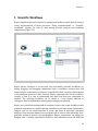
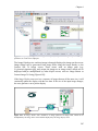
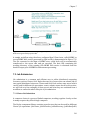
1.1 What is Kepler?
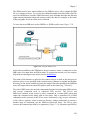
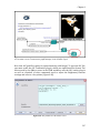
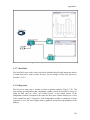
Kepler is a software application for the analysis and modeling of scientific data.
Using Kepler's graphical interface and components, scientists with little background
in computer science can create executable scientific workflows, which are flexible
tools for accessing scientific data (streaming sensor data, medical and satellite
images, simulation output, observational data, etc.) and executing complex analysis
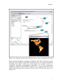
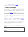
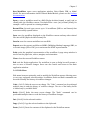
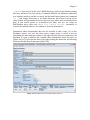
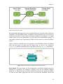
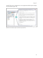
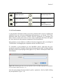
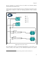
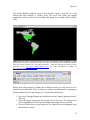
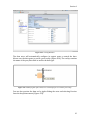
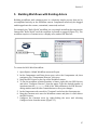
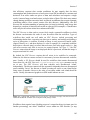
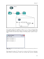
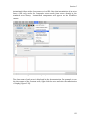
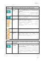
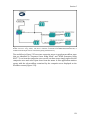
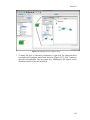
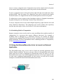
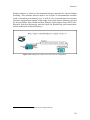
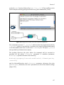
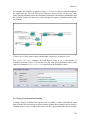
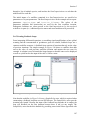
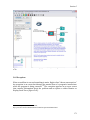
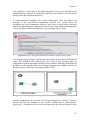
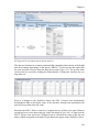
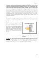
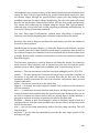
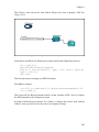
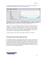
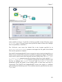
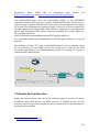
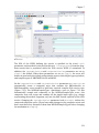
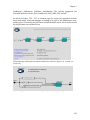
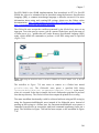
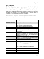
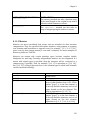
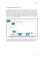
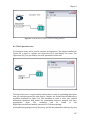
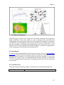
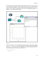
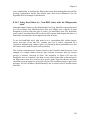
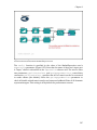
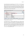
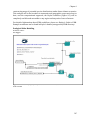
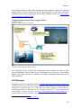
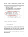
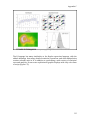
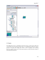
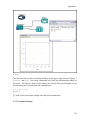
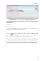
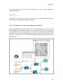
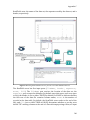
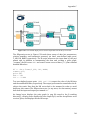
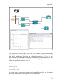
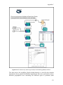
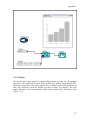
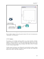
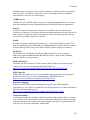
on the retrieved data (Figure 1.1).
6
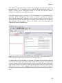
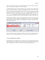
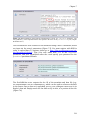
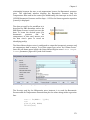
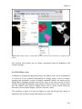
Chapter 1
Figure 1.1 A scientific workflow (GARP_SingleSpecies_BestRuleSet-IV.xml) displayed in the Kepler
interface. This workflow processes species occurrence data to create an ecological niche model.
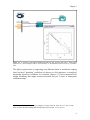
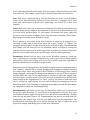
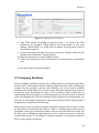
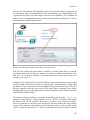
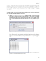
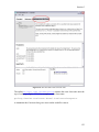
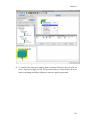
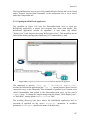
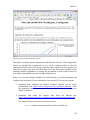
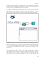
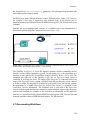
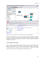
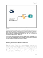
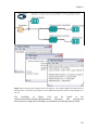
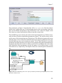
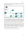
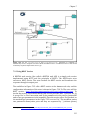
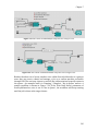
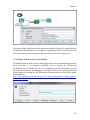
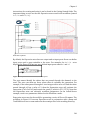
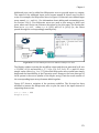
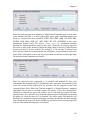
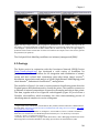
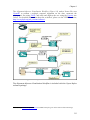
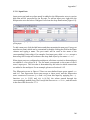
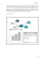
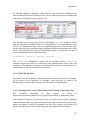
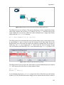
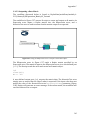
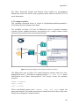
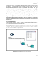
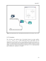
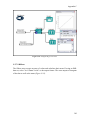
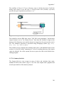
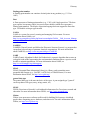
Kepler includes distributed computing technologies that allow scientists to share
their data and workflows with other scientists and to use data and analytical
workflows from others around the world. Kepler also provides access to a
continually expanding, geographically distributed set of data repositories,
computing resources, and workflow libraries (e.g., ecological data from field
stations, specimen data from museum collections, data from the geosciences, etc.)
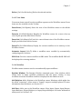
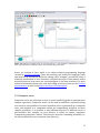
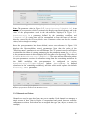
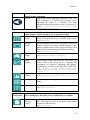
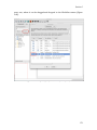
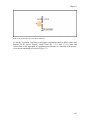
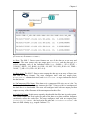
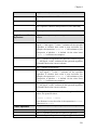
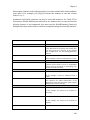
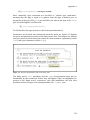
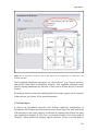
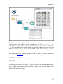
(Figure 1.2).
7
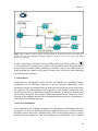
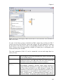
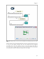
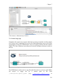
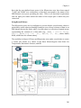
Chapter 1
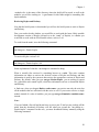
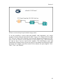
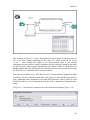
Figure 1.2: A workflow (eml-simple-linearRegression-R.xml) that performs and plots a simple linear
regression on a meteorological data set stored remotely on the EarthGrid and accessed via a workflow
actor.
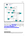
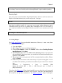
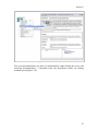
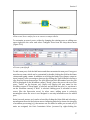
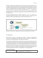
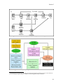
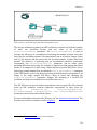
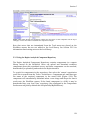
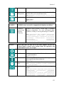
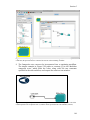
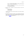
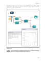
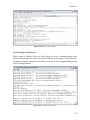
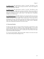
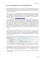
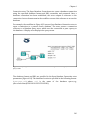
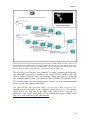
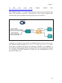
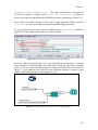
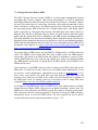
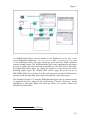
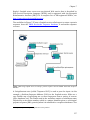
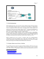
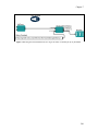
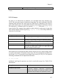
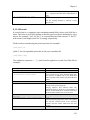
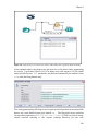
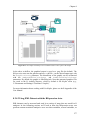
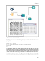
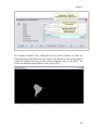
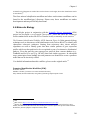
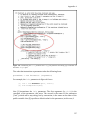
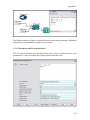
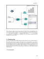
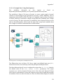
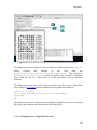
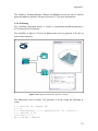
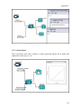
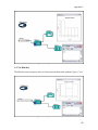
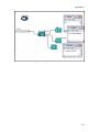
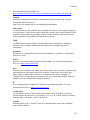
The Kepler system aims at supporting very different kinds of workflows, ranging
from low-level “plumbing” workflows of interest to Grid engineers, to analytical
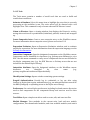
knowledge discovery workflows for scientists (Figure 1.3), and conceptual-level
design workflows that might become executable only as a result of subsequent
refinement steps.1
1
Ludäscher, B., I. Altintas, C. Berkley, D. Higgins, E. Jaeger-Frank, M. Jones, E. Lee, J. Tao, Y. Zhao.
2005. Scientific Workflow Management and the Kepler System, DOI: 10.1002/cpe.994
8
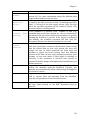
Chapter 1
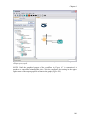
Figure 1.3: The Promoter Identification Workflow, a typical scientific knowledge discovery workflow that
links genomic biology techniques such as microarrays with bioinformatics tools such as BLAST to identify
and characterize eukaryotic promoters.
Kepler builds upon the mature Ptolemy II framework, developed at the University of
California, Berkeley. Other scientific workflow environments include academic
systems such as SCIRun, Triana, Taverna, and commercial systems
(Scitegic/Pipeline-Pilot, Inforsense/Accelrys).2 For a detailed discussion of these
and
other
workflow
systems,
please
see
http://www.gridbus.org/reports/GridWorkflowTaxonomy.pdf.
1.1.1 Features
Altintas, I, C. Berkley, E. Jaeger, M. Jones, B. Ludäscher, S. Mock, Kepler: An Extensible System for
Design and Execution of Scientific Workflows, system demonstration, 16th Intl. Conf. on Scientific
and Statistical Database Management (SSDBM'04), 21-23 June 2004, Santorini Island, Greece.
2
9
Chapter 1
Using Kepler, scientists can capture workflows in a format that can easily be
exchanged, archived, versioned, and executed. Both Kepler’s intuitive GUI (inherited
from Ptolemy) for design and execution, and its actor-oriented modeling paradigm
make it a very versatile tool for scientific workflow design, prototyping, execution,
and reuse for both workflow engineers and end users. Kepler workflows can be
exchanged in XML using Ptolemy’s own Modeling Markup Language (MoML). Kepler
currently provides the following features: 3
Access to Scientific Data: The Kepler component library contains an Ecological
Metadata Language (EML) ingestion actor (EML2Dataset) used to access, download,
and preview EML described data sources. The EML2Dataset actor allows Kepler to
import a multitude of heterogeneous data, making it a very flexible tool for
scientists who often deal with many data and file formats. A similar actor exists for
Darwin Core-described data sets (DarwinCoreDataSource). In addition, Kepler's
ReadTable actor allows users to access and incorporate data stored in Excel files.
Graphical User Interface: Users can build workflows via Kepler's intuitive
graphical interface. Components are dragged and dropped onto a Workflow canvas,
where they can be connected, customized, and then executed.
Distributed Execution (Web and Grid-Services): Kepler’s Web and Grid service
actors allow scientists to utilize computational resources on the net in a distributed
scientific workflow. Kepler’s generic WebService actor provides the user with an
interface to seamlessly plug in and execute any WSDL-defined Web service. In
addition to generic Web services, Kepler also includes specialized actors for
executing jobs on the Grid, e.g., actors for certificate-based authentication (SProxy or
GlobusProxy), Grid job submission (GlobusJob), and Grid-based data access
(GridFTP). Third-party data transfer on the Grid can be established using GridFTP
and SRB (Storage Resource Broker) actors.
Prototyping Workflows: Kepler allows scientists to prototype workflows before
implementing the actual code needed for execution. Kepler’s Composite actor can be
used as a “blank slate” that prompts the scientist for critical information about an
actor, e.g., the actor’s name and port information.
Searchable Libraries: Kepler has a searchable library of actors and data sources
(found under the Components and Data tabs of the application) with numerous
reusable Kepler components and an ever-growing collection of data sets.
Database Access and Querying: Kepler includes database actors, such as the
DBConnect actor, which emits a database connection token (after user login) to be
used by any downstream DBQuery actor that needs it.
3
Ibid.
10
Chapter 1
Other Execution Environments: Supporting foreign language interfaces via the
Java Native Interface (JNI) gives the user flexibility to reuse existing analysis
components and to target appropriate computational tools. For example, Kepler
(through Ptolemy) already includes a Matlab actor. Actors that execute R code
(RExpression, Correlation, RMean, RMedian, and others) are also included in the
standard actor library. Any application that can be executed on the command line
can also be executed by the Kepler CommandLineExec actor.
Data Transformation: Kepler includes a suite of data transformation actors (XSLT,
XQuery, Perl, etc.) for linking semantically compatible but syntactically incompatible
Web services together.
Flexible Execution: The BrowserUI actor is used for injecting user control and
input, as well as output of legacy applications anywhere in a workflow via the user’s
Web browser. Kepler workflows can also be run in batch mode using Ptolemy’s
background execution feature.
Configurable Libraries: Users can configure their own actor libraries via a
semantic type interface, or download (and upload) additional actors from the Kepler
repository. Actors can be created and added to the local library by semantically
annotating them, using a Seman
1.1.2 Architecture
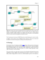
Kepler builds upon the mature Ptolemy II framework, developed at the University of
California, Berkeley. Ptolemy II is a software framework developed as part of the
Ptolemy project, which studies modeling, simulation, and design of concurrent, realtime, embedded systems. Kepler 2.4 is based on Ptolemy II 9.1.
Kepler inherits from Ptolemy the actor-oriented modeling paradigm that separates
workflow components ("actors") from the overall workflow orchestration (conducted by
"directors"), making components more easily reusable. Through the actor-oriented and
hierarchical modeling features built into Ptolemy, Kepler scientific workflows can
operate at very different levels of granularity, from low-level "plumbing workflows" (that
explicitly move data around or start and monitor remote jobs, for example) to high-level
"conceptual workflows" that interlink complex, domain-specific data analysis steps.
Kepler also inherits modeling and design capabilities from Ptolemy, including the Vergil
graphical user interface and workflow scheduling and execution capabilities.
Kepler extensions to Ptolemy include an ever increasing number of components (called
"actors") aimed particularly at scientific applications: remote data and metadata access,
data transformations, data analysis, interfacing with legacy applications, Web service
invocation and deployment, and provenance tracking, among others. Target application
areas include bioinformatics, computational chemistry, ecoinformatics, and
geoinformatics.
11
Chapter 1
Ptolemy/Vergil (A Very Brief Overview)
Ptolemy II, developed at the University of California, Berkeley, is an open-source
software framework developed as part of the Ptolemy project. Ptolemy II is a Java-based
component assembly framework with a graphical user interface called Vergil.
The Ptolemy project studies modeling, simulation, and design of concurrent, realtime, embedded systems. The focus is on embedded systems, particularly those that
mix technologies including, for example, analog and digital electronics, hardware
and software, and electronics and mechanical devices. The focus is also on systems
that are complex in the sense that they mix widely different operations, such as
networking, signal processing, feedback control, mode changes, sequential decision
making, and user interfaces.4
Ptolemy II takes a component view of design, in that models are constructed as a set
of interacting components. A model of computation governs the semantics of the
interaction, and thus imposes a discipline on the interaction of components.5
Ptolemy II offers a unified infrastructure for implementations of a number of models
of computation. The overall architecture consists of a set of packages that provide
generic support for all models of computation and a set of packages that provide
more specialized support for particular models of computation. Examples of the
former include packages that contain math libraries, graph algorithms, an
interpreted expression language, signal plotters, and interfaces to media capabilities
such as audio. Examples of the latter include packages that support clustered graph
representations of models, packages that support executable models, and domains,
which are packages that implement a particular model of computation.6
The Vergil GUI is a visual editor written in Java. Using Vergil, users can graphically
construct and run scientific workflows. For more information about Vergil, see the
Ptolemy documentation.
Modeling Markup Language (MoML)
Modeling Markup Language (MoML), the primary persistent file format for Ptolemy
II models, is an Extensible Markup Language (XML) schema. It is intended
4
Hylands, Christopher, Edward Lee, Jie Liu, Xiaojun Liu, Stephen Neuendorffer, Yuhong Xiong, Yang
Zhao, Haiyang Zheng, Ptolemy Overview,
http://www.ptolemy.eecs.berkeley.edu/publications/papers/03/overview/overview03.pdf
5
Ibid.
6
Ibid.
12
Chapter 1
for specifying interconnections of parameterized components, and is the primary
mechanism for constructing models whose definition and execution is distributed
over the network.7
The key features of MoML include:8
• Web integration. MoML is an XML schema intended for use on the Internet. File
references are via URIs (in practice, URLs), both relative and absolute, so MoML is
equally comfortable working in applets and applications.
• Implementation independence. MoML is designed to work with a variety of
modeling tools.
• Extensibility. Components can be parameterized in two ways. First, they can have
named properties with string values. Second, they can be associated with an
external configuration file that can be in any format understood by the component.
Typically, the configuration will be in some other XML schema, such as PlotML or
SVG (scalable vector graphics).
• Classes and inheritance. Components can be defined in MoML as classes which can
then be instantiated in a model. Components can extend other components through
an object-oriented inheritance mechanism.
• Semantics independence. MoML defines no semantics for an interconnection of
components. It represents only the hierarchical containment relationships between
entities with properties, their ports, and the connections between their ports. In
Ptolemy II, the meaning of a connection (the semantics of the model) is defined by
the director for the model, which is a property of the top level entity. The director
defines the semantics of the interconnection. MoML knows nothing about directors
except that they are instances of classes that can be loaded by the class loader and
assigned as properties.
For detailed information about MOML and its syntax, please see the Ptolemy user
manual, Chapter 7.
1.2 History of the Kepler Project
Kepler was founded in 2002 by researchers at the National Center for Ecological
Analysis and Synthesis (NCEAS) at University of California Santa Barbara, the San
Diego Supercomputer Center (SDSC) at University of California San Diego, and the
University of California Davis as part of the Science Environment for Ecological
Knowledge (SEEK) and Scientific Data Management (SDM) projects. The Kepler
7
8
Ptolemy User Manual, http://www.eecs.berkeley.edu/Pubs/TechRpts/2007/EECS-2007-7.pdf
Ibid.
13
Chapter 1
software extends the Ptolemy II system developed by researchers at the University of
California Berkeley. Although not originally intended for scientific workflows, Ptolemy
II provides a mature platform for building and executing workflows, and supports
multiple models of computation.
An alpha version of the Kepler software was released in April of 2005. Three beta
versions followed: beta1, June 2006; beta2, July 2006; and beta3, January 2007. The first
official release, Version 1, was released on May 2, 2008. Version 2.0.0 was released in
June 2010 with major improvements to the GUI, modular design and KAR handling.
Version 2.1.0 was released Sep 30, 2010, and contained new features and bug-fixes.
Version 2.2.0 was released June 14, 2011, improving memory usage, and fixing many
bugs. Version 2.3.0 was released Jan 20, 2012, improving the GUI and fixing many bugs.
Version 2.4.0 is expected to be released in March 2013.
Kepler is an open collaboration with many contributors from diverse domains of science
and engineering, including ecology, evolutionary biology, molecular biology, geology,
chemistry, computer science, electrical engineering, oceanography, and others. Members
from the following projects are currently contributing to the Kepler project:












SEEK: Science Environment for Ecological Knowledge
SDM Center/SPA: SDM Center/Scientific Process Automation
Ptolemy II: Heterogeneous Modeling and Design
GEON: Cyberinfrastructure for the Geosciences
ROADNet: Real-time Observatories, Applications, and Data Management
Network
EOL: Encyclopedia of Life
Resurgence
CIPRes: CyberInfrastructure for Phylogenetic Research
REAP: Realtime Environment for Analytical Processing
Kepler/CORE: Development of a Comprehensive, Open, Reliable, and
Extensible Scientific Workflow Infrastructure
CAMERA: Community Cyberinfrastructure for Advanced Microbial Ecology
Research & Analysis
bioKepler: A Comprehensive Bioinformatics Scientific Workflow Module for
Distributed Analysis of Large-Scale Biological Data
Contributing members jointly determine the goals for Kepler as well as contribute to the
design and implementation of the software system. We welcome contributions and
encourage other people and projects to join as contributing members. For more
information about contributing to Kepler, please see Section 1.5.
Some Kepler members receive support from various grants, including but not limited to:
the National Science Foundation under awards 0225676 for SEEK, 0225673
(AWSFL008-DS3) for GEON, 0619060 for REAP, 0722079 for Kepler/CORE, 1062565
for bioKepler, and 0941692 for DISCOSci; the Gordon and Betty Moore Foundation
award to Calit2 at UCSD for CAMERA; by the Department of Energy under Contract
14
Chapter 1
No. DE-FC02-01ER25486 for SciDAC/SDM; and by DARPA under Contract No.
F33615-00-C-1703 for Ptolemy.
Work was conducted with logistical support from the National Center for Ecological
Analysis and Synthesis, a Center funded by NSF (Grant #DEB-0553768), the University
of California, Santa Barbara, and the State of California.
Ptolemy receives support in part by the Center for Hybrid and Embedded Software
Systems (CHESS) at UC Berkeley, which receives support from the National Science
Foundation (NSF awards #0720882 (CSR-EHS: PRET), #1035672 (CPS: Medium:
Ptides), and #0931843 (CPS: Large: ActionWebs)), the Naval Research Laboratory
(#NOOI73-12-1-G015), the Multiscale Systems Center (MuSyC), one of six research
centers funded under the Focus Center Research Program, a Semiconductor Research
Corporation program, and the following companies: Bosch, National Instruments, and
Toyota. In the past, CHESS has been sponsored by Agilent, DGIST, General Motors,
Hewlett Packard, Infineon, and Microsoft.
Ptolemy is also supported in part by the TerraSwarm Research Center, one of six centers
supported by the STARnet phase of the Focus Center Research Program (FCRP) a
Semiconductor Research Corporation program sponsored by MARCO and DARPA.
Ptolemy is also supported in part by the Naval Research Laboratory project, "Software
Producibility for System of Systems," and was accomplished under Cooperative
Agreement Number NOOI73-12-1-G015.
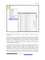
1.3 Kepler Code Contributors
The following people have made contributions to the Kepler code. Contributors are listed
in chronological order of commits to the SVN repository:
Matthew Jones
Chad Berkley
Ilkay Altintas
Zhengang Cheng
Efrat Frank
Bertram Ludaescher
Jing Tao
Steve Mock
Xiaowen Xin
Dan Higgins
Yang Zhao
Christopher Brooks
Tobin Fricke
Rod Spears
15
Chapter 1
Werner Krebs
Shawn Bowers
Laura Downey
Wibke Sudholt
Timothy McPhillips
Bing Zhu
Nandita Mangal
Jagan Kommineni
Jenny Wang
John Harris
Kevin Ruland
Matthew Brooke
Oscar Barney
Vitaliy Zavesov
Zhije Guan
Norbert Podhorszki
Samantha Katz
Tristan King
Josh Madin
Kirsten Menger-Anderson
Edward Lee
Daniel Crawl
Derik Barseghian
Lucas Gilbert
Nathan Potter
Ben Leinfelder
Carlos Rueda
Jim Regetz
Sean Riddle
Aaron Schultz
David Welker
Mark Schildhauer
Debi Staggs
Jianwu Wang
Sven Koehler
Faraaz Sareshwala
Daniel Zinn
Madhusudan
Chandrika Sivaramakrishnan
Lei Dou
Merve Ildeniz
Gongjing Cao
Manish Anand
Marcin Plociennik
Tomasz Zok
Michal Owsiak
16
Chapter 1
Contributions to Kepler are welcome. Please see Section 1.5 for details on how to
contribute. Thanks.
1.4 Future Goals
The Kepler project is an ongoing collaboration, and we will continue to refine,
release, and support the Kepler software. Our aim is to improve and enhance the
Kepler scientific workflow system to yield a comprehensive, open, reliable, and
extensible scientific workflow infrastructure suitable for serving a wide variety of
scientific communities.
The goal of future Kepler development is to (i) enable multiple groups in a number
of distinct disciplines to easily create, support, and make available domain-specific
Kepler extensions; (ii) better support those crucial features that are needed by all
disciplines; and (iii) provide for the wide range of deployment scenarios required by
different disciplines and distinct research settings.
More specifically, future goals include making Kepler:
Independently Extensible. Rather than enforcing conventions that might slow
progress in the various disciplines contributing to Kepler, we plan to further enable
independent extensibility of Kepler while making it easy to package domain-specific
contributions in a way that ensures both the stability of the overall system and
clearly indicates what components are expected to work well together.
With the 2.0 release of Kepler, we have created a module system that allows us to
separate Kepler base system functionality from domain-specific extensions. We
have divided Kepler into a set of mandatory modules (the kepler suite); a set of
extension modules that communicate with the kernel via well-defined and generic
extension interfaces; and a number of actor modules for distinct disciplines. We
developed a configuration management system to support downloading, installing,
and updating the Kepler distribution and a Module Manager for discovering and
installing standard and 3rd-party modules and specifying modules to be employed
during execution. With this architecture, third-parties can now develop alternative
modules with additional capabilities suitable for particular science domains.
Consistently Reliable: Reliability for developers and users alike ensures that
Kepler can be applied confidently as dependable cyberinfrastructure. We are
working to ensure run-time reliability (both for when Kepler is used as a desktop
research application and as middleware that other domain-specific applications can
build upon). Our approach of dividing Kepler into the Kepler kernel and extension
set will enable other development teams to freely develop new modules and actor
17
Chapter 1
packages as needed without endangering the stability of the kernel, and even to
replace standard extensions as needed.
Open Architecture, Open Project. We will disseminate plans, designs, and system
documentation as we develop them and provide mechanisms for suggestions and
feedback throughout the course of the project. We will also actively engage the user
community and gather requirements, advice, and feedback on priorities, both from
those already committed to using Kepler (i.e., the Kepler “stakeholders”), and from
scientists who could benefit.
Comprehensive (End-to-End) System. We plan to widen the scope of Kepler by
providing new, fundamental enhancements that will benefit all user communities:
enhancing Kepler with new and improved generic capabilities for data, service, and
workflow management. More specifically, we are working on new and more
comprehensive systems for:

Data Management. We plan to support data management tasks in a generic
way within the Kepler framework so that all data management tasks (e.g.,
controlling and managing the flow of data into and out of workflows,
comparing and visualizing data and metadata, converting data formats, and
managing data references) are handled transparently by the workflow
execution framework rather than by special-purpose actors.

External Service and Grid Management. Currently, Kepler workflows that
make extensive use of external services generally use actor-oriented
approaches for managing and accessing those services. We are working to
better enable the system to carry out computations on the optimal set of
computing resources at run time, based on resource availability and
preferences; and to make it easier for users to share and redeploy workflows
in different environments. In addition, we are working on integrated support
for managing authentication and authorization information.

Workflow Management. Our goal is for Kepler to provide comprehensive
support for end-to-end workflow management—from initial prototyping to
workflow execution. We are working to make the application aware of the
scientific context in which workflows are being run, the flow of data through
and across successive workflows (as is common in scientific research), and
the origin of workflows. In addition, we will continue to improve support for
common workflow management tasks such as designing, storing, and
validating individual workflows; organizing workflows, data, and results
within the context of a particular project or research study; and capturing
and querying the provenance of workflows and data. The Kepler workflowrun-manager and provenance modules will provide a whole new suite of
functionality for managing workflows.
18
Chapter 1
Please see the Kepler/CORE Web page for detailed information about specific
features that are under development, and/or the Bug base for more features that we
are adding and improving in the coming months.
1.5 Participating in Kepler Development
Kepler is an open source cross-project collaboration, and we welcome contributions
of all types. Participants can get involved by joining a mailing list (either for
developers or users), participating in IRC chat, or getting a Kepler SVN account to
view or contribute to the Kepler source.
Individuals can join the kepler-dev mailing list to interact with the rest of the
development team or the kepler-users mailing list to request and/or exchange user
support. The current list of subscribers is available only to list members and can be
viewed (after subscription) at the mailing list info page.
Many of the Kepler developers use IRC to chat on a daily basis. We use the '#kepler'
channel on irc.ecoinformatics.org:6667 for our discussions. More details on how to
use IRC can be found on the SEEK IRC page.
The code for Kepler is managed in an SVN repository. Read-only access is open for all.
If you need to write to the SVN repository, please visit https://keplerproject.org/developers for instructions. You can use any SVN client to access the Kepler
repository.
To check out and build the Kepler source code, you will need to be running Java 1.6 or
later, Ant 1.7.1, and have installed an SVN client, v1.5. For development with Eclipse
these have been tested with Eclipse Ganymede and SVN 1.6, with Subclipse 1.4.7.
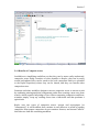
Downloading the Build
To download the latest version of the build from the repository, you will want to create a
new directory and then execute the svn checkout (co) command as in the following
example.
mkdir <modules.dir>
cd <modules.dir>
svn co https://code.kepler-project.org/kepler/trunk/modules/build-area
cd build-area
19
Chapter 1
<modules.dir> is the name of the directory where the build will be stored, as well as the
modules you will be working on. A good name for this folder might be something like
kepler.modules.
Retrieving Kepler and Ptolemy
Now that the build system is downloaded you will use the build system to retrieve Kepler
and Ptolemy.
First, you need to decide whether you would like to work with the latest, likely unstable
development version of Kepler (referred to as the “trunk” of Kepler), or whether you
would like to work with an official stable release, such as 2.4.0.
To work from the trunk, issue the following command:
ant change-to –Dsuite=kepler
To retrieve Kepler version 2.4.0:
ant change-to –Dsuite=kepler-2.4.0
Some explanation of what the “ant change-to command is doing:
What is actually first retrieved is something known as a suite. This suite contains
information on where to retrieve the desired versions of Kepler and Ptolemy and that
information is used by the system to then retrieve the appropriate versions of Kepler and
Ptolemy. By default, when you type ant get -Dsuite=kepler, you are making a request
for a particular suite named kepler, which has information on how to download Kepler
and Ptolemy.
A final note, when you do get -Dsuite=<suite.name> you retrieve not only the suite, but
all the modules that are associated with the suite as well. If you want to retrieve a single
module instead of a suite of modules, you just type ant get -Dmodule=<module.name>
instead.
Note:
If you are behind a firewall and do not have access to port 22 and you are working off the
trunk, then the download of Ptolemy will fail when you execute the "ant change-to Dsuite=kepler" command. In this case, you must download Ptolemy manually using the
following command:
20
Chapter 1
svn co https://source.eecs.berkeley.edu/svn/chess/ptII/trunk <kepler.modules>/ptolemy
Running Kepler
Now that you have downloaded the Kepler Build System and have used it to retrieve the
Kepler version that interests you, you are ready to run. Just type:
ant run
Note that it would be possible for a new user to get started without having to enter a
command between get and run by chaining these commands in ant. So, for example, if
you wanted to download and run Kpler from the trunk all in one command, you could
type:
ant change-to –Dmodule=kepler run
1.5.1 Using Eclipse
See Kepler and Eclipse for more detailed instructions. However, in most cases, these
instructions should be adequate.
1. Type ant eclipse.
2. Open Eclipse in a new or existing workspace.
3. Choose File->Import... Under the General folder, choose Existing Projects
into Workspace. Click Next.
4. Click Browse right next to the Select root directory: field. Go to and select
the <module.dir> directory where you saved the build and downloaded your
modules. Click Choose.
5. The projects that were generated will be automatically detected by Eclipse.
Click on Finish.
6. KarDoclet.java uses doclet code from tools.jar. If you are using Java 1.6 on a
non-Mac OS X machine, you will need to add tools.jar to the list of external
jars:
Windows
->
Preferences
->
Java
->
Installed
JREs
Select the default JRE -> Edit -> Add External Jars -> [Path to
JDK]/lib/tools.jar
If you have the Subversive Eclipse plugin installed you can select the newly generated
projects, right click on them and choose "Share Projects" and follow the instructions in
the wizard to set up the connection to the Kepler repository (https://code.kepler-
21
Chapter 1
project.org/code/kepler/). Repeat the process for the ptolemy project using the Ptolemy
repository (svn://source.eecs.berkeley.edu/chess/ptII/).
If you have the Subversive plugin installed, see Updating the local copy of the Kepler
sources
To run kepler, create a new Java Application Run Configuration: with project: loader,
Main class: org.kepler.Kepler
These instructions and further reference detail, including how to run a workflow from the
command line, and setting system properties, and other details can be found at: Kepler
Build System Instructions and Overview.
1.5.2 Contributing to Kepler
In order to contribute directly to Kepler, one must use a named account to enable you to
make changes to the web site or the SVN repositories. In general, people with write
access should only make changes to modules with which they are directly involved or
that they have discussed with the relevant Infrastructure and Development Teams. Please
be sure you have contacted the appropriate Team(s) before you request an account.
To request a named account, send an email to [email protected] with your name,
association and a brief description of your project needs.
1.6 Reporting Bugs
The Kepler project uses Bugzilla for reporting bugs as well as for sharing future
development plans. Please register yourself by creating a new bugzilla account to
participate in future plans, bug reports, and updates. Note that you need to have an
ecoinformatics.org account to be able to register.
Bugzilla is one example of a class of programs called "Defect Tracking Systems", or,
more commonly, "Bug-Tracking Systems". Defect Tracking Systems allow individual or
groups of developers to keep track of outstanding bugs in their product effectively.
1.7 Further Reading
As part of the outreach effort for Kepler, we have produced a variety of documents and
publications. Publications of interest include:

Scientific Workflow Management and the Kepler System, B. Ludäscher, I.
Altintas, C. Berkley, D. Higgins, E. Jaeger-Frank, M. Jones, E. Lee, J. Tao, Y.
Zhao, Concurrency and Computation: Practice & Experience, 18(10), pp. 10391065, 2006.
22
Chapter 1
Additional publications are listed on the Kepler web site at http://keplerproject.org.
Independent publications of the collaborating projects can be reached at their main
websites: SEEK, SDMCenter-SPA, KBIS-SPA, Ptolemy, GEON, bioKepler, and
CAMERA.
23
2. Installing and Running Kepler
2.1 System Requirements
Recommended system requirements for Kepler:






300 MB of disk space
512 MB of RAM minimum, 1 GB or more recommended
2 GHz CPU minimum
Java 1.6
Network connection (optional). Although a connection is not required to run
Kepler, many workflows require a connection to access networked
resources.
R software (optional). R is a language and environment for statistical
computing and graphics, and it is required for some common Kepler
functionality.
Java
1.6
is
required
and
can
be
obtained
online
at:
http://www.oracle.com/technetwork/java/javase/downloads/index.html or from
your system administrator.
Kepler has many actors that utilize R, so installing R is recommended:
http://www.r-project.org/.
2.2 Installing Kepler
Kepler is an open-source, cross-platform software program that can run on
Windows, Macintosh, or Linux-based platforms. Instructions for each platform are
contained in the following sections.
2.2.1 Installing on Windows
Follow these steps to download and install Kepler for Windows.
Java
1.6
is
required
and
can
be
obtained
online
at:
http://www.oracle.com/technetwork/java/javase/downloads/index.html or from
your system administrator.
24
Chapter 2
Kepler has many actors that utilize R, so installing R is recommended:
http://www.r-project.org/.
1. Click the following link: https://kepler-project.org/users/downloads and
select the Windows installer.
2. Save the install file to your computer.
3. Double-click the install file to open the install wizard. We recommend that
you quit all programs before continuing with the installation. You can cancel
the installation at any point via the Quit button in the lower right corner of
the installer. To proceed with the installation, click the Next button.
4. Click the Next button. An information screen containing notes about the
application appears. Click Next once you have read through the information
to select an installation path. By default, the software will be installed in
C:\Program Files\Kepler-x.y. The installer will create the target directory if it
does not yet exist. If the directory already exists, the installer will confirm the
location before possibly overwriting an existing version.
5. Choose the packs to install. Once you have selected an installation, click the
Next button.
6. The Kepler installer displays a status bar as the installation progresses. If
Kepler has previously been installed on the system, the installer will
overwrite any existing cache files.
Once the installation is complete, a confirmation
screen opens. An uninstaller program is also created in
the installation location. A Kepler shortcut icon will
appear on your desktop.
2.2.3 Installing on Macintosh
The Mac installer will install the Kepler application on your system. Java is included
as part of the Mac OSX operating system, so it need not be installed.
Kepler has many actors that utilize R, so installing R is recommended:
http://www.r-project.org/.
Follow these steps to download and install Kepler for Macintosh systems:
Chapter 2
1 Click the following link: https://kepler-project.org/users/downloads and
select the Mac install file. Save the install file to your computer.
2 Double-click the install icon that appears on your desktop when the
extraction is complete.
3 Follow the steps presented in the install wizard to complete the Kepler
installation process.
A Kepler icon is created under /Applications/Kepler-x.y. The icon can be dragged
and dropped to the desktop or the dock if desired.
2.2.4 Installing on Linux
The Linux installer will install the Kepler application.
Java
1.6
is
required
and
can
be
obtained
online
at:
http://www.oracle.com/technetwork/java/javase/downloads/index.html or from
your system administrator.
Kepler has many actors that utilize R, so installing R is recommended:
http://www.r-project.org/.
Follow these steps to download and install Kepler for Linux:
1. Click the following link: https://kepler-project.org/users/downloads and
select the Linux install file.
2. Save the install file to your computer
3. Double-click the install file to open the install wizard. If double-clicking the
install file doesn’t work on your system, you may run the command java –
jar installer-file-name in a terminal to open the install wizard. We
recommend that you quit all programs before continuing with the
installation.
4. The Kepler installer displays a status bar as the installation progresses. If
Kepler has previously been installed on the system, the installer will
overwrite any existing cache files.
2.3 Starting Kepler
To start Kepler on a PC, double-click the Kepler shortcut icon on the desktop. Kepler
can also be started from the Start menu. Navigate to Start menu > All Programs, and
select "Kepler" to start the application. On a Mac, the Kepler icon is created under
Chapter 2
Applications/Kepler-x.y. The icon can be dragged and dropped to the desktop or the
dock if desired.
To start Kepler on a Linux machine, use the following steps:
1. Open a shell window. On some Linux systems, a shell can be opened by rightclicking anywhere on the desktop and selecting "Open Terminal". Speak to
your system administrator if you need information about your system.
2. Navigate to the directory in which Kepler is installed. To change the
directory, use the cd command (e.g., cd directory_name).
3. Type ./kepler.sh to run the application.
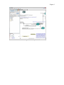
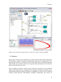
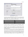
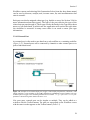
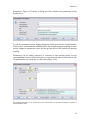
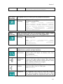
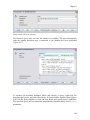
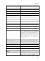
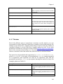
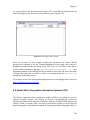
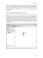
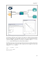
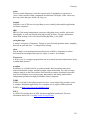
The main Kepler application window opens (Figure 2.1). From this window you can
access and run existing scientific workflows and/or create your own custom
scientific workflow. Each time you open an existing workflow or create a new
workflow, a new application window opens. Multiple windows allow you to work
on several workflows simultaneously and compare, copy, and paste components
between workflows.
To start Kepler from the command line (optionally loading a workflow), use the
following command:
kepler.sh [-nosplash] [workflow.xml | workflow.kar]
-nosplash
start without showing splash screen.
On Windows, the executable is kepler.bat instead of kepler.sh.
To run a workflow XML from the command line:
kepler -runwf [-nogui | -redirectgui dir] [-nocache]
[-noilwc] [-param1 value1 ...] workflow.xml
-nogui
-nocache
-noilwc
-redirectgui dir
run without GUI support.
run without kepler cache.
run without incrementing LSIDs when the
workflow changes.
redirect the contents of GUI actors to
the specified directory.
To run a workflow KAR from the command line:
kepler.sh -runkar [-nogui | -redirectgui dir] [-force]
[-param1 value1 ...] workflow.kar
Chapter 2
-force
-nogui
-redirectgui dir
attempt to run ignoring missing module
dependencies.
run without GUI support.
redirect the contents of GUI actors to
the specified directory.
You can specify the values of workflow parameters:
kepler.sh -runwf -x 4 -y "foo" workflow.xml
The above command runs 'workflow.xml', setting the parameters x = 4 and
y = "foo".
The full command-line usage for the Kepler executable can be found by running:
kepler.sh -h
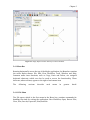
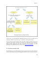
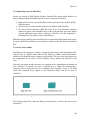
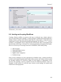
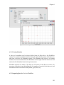
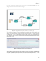
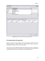
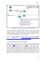
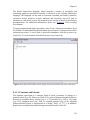
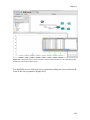
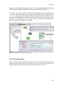
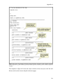
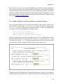
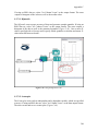
2.4 The User Interface
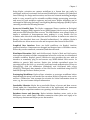
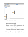
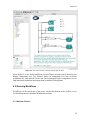
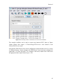
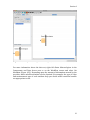
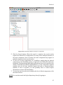
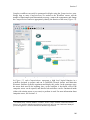
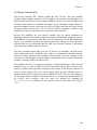
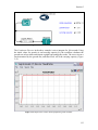
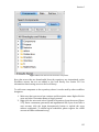
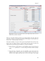
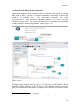
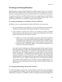
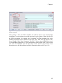
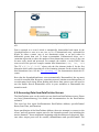
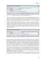
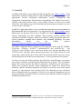
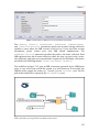
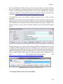
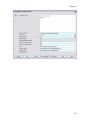
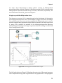
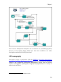
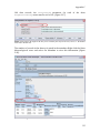
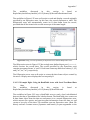
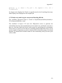
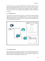
Scientific workflows are edited and built in Kepler’s easily navigated, drag-and-drop
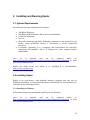
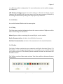
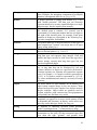
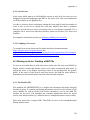
interface. The major sections of the Kepler application window (Figure 2.1) consist
of the following:





Menu bar – provides access to all Kepler functions.
Toolbar – provides access to the most commonly used Kepler functions.
Components, Data Access, and Outline area – consists of a Components tab. ,
a Data tab, and an Outline tab. The Components tab, and the Data tab both
contain a search function and display the library of available components
and/or search results. The Outline tab displays an outline of components that
are in your current workflow.
Workflow canvas – provides space for displaying and creating workflows.
Navigation area – displays the full workflow. Click a section of the workflow
displayed in the Navigation area to select and display that section on the
Workflow canvas.
Each of these interface areas is described in more detail in the following sections.
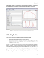
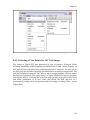
Chapter 2
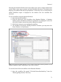
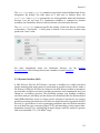
Figure 2.1: Empty Kepler window with major sections annotated.
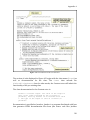
2.4.1 Menu Bar
Running horizontally across the top of the Kepler application, the Menu bar contains
the seven Kepler menus: File, Edit, View, Workflow, Tools, Window, and Help.
Common menu item functions, such as Copy, Paste and Delete, are assigned
keyboard shortcuts, which can also be used to access the functionality. These
shortcuts, when relevant, appear to the right of each menu item.
The
following
sections
describe
each
menu
in
greater
detail.
2.4.1.1 File Menu
The File menu, which is the first menu in the Menu bar, contains commands for
handling files and for exiting the application: New Workflow, Open, Recent Files,
Close, Save, Save As, Export As, Print, and Exit.
Chapter 2
New Workflow: open a new application window. Select Blank, FSM, or Modal
Model. For more information about FSM and Modal Models, please see the Ptolemy
documentation.
Open…: open a workflow saved in a KAR (Kepler Archive format) or xml (.xml or
.moml) onto the Workflow canvas. Text-based files—text (.txt) or html (.html), for
example—will be opened in a viewing window.
Recent Files: list and open recent up to 10 workflows (KAR or xml format) that
were successfully opened before.
Save: save the workflow displayed on the Workflow canvas and any other related
files into a KAR (Kepler Archive format) file.
Save As: save the current workflow to a new KAR.
Export: save the current workflow as MOML (MOdeling Markup Language) XML, or
to a static image (GIF or PNG), or to an interactive HTML representation.
Print: print the graphical representation of the workflow. A page setup window is
used to set the paper size, source, margins, and orientation.
Close: close the current Workflow canvas.
Exit: exit the Kepler application. If a workflow is open, a dialog box will prompt a
user to save or discard changes. Users can also cancel and return to the main
application window.
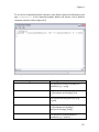
2.4.1.2 Edit Menu
Edit menu items are primarily used to modify the Workflow canvas, allowing users
to cut, copy, and paste selected entities. In addition, Undo and Redo commands can
be used to modify the history of workflow changes.
Undo: (Ctrl+Z) Undo the most recent change. The "Undo" command can be performed
multiple times to undo the history of workflow changes. The size of the history buffer
is limited only by available RAM.
Redo: (Ctrl+Y) Redo the most recent change. The "Redo" command can be
performed multiple times to redo the history of workflow changes.
Cut: (Ctrl+X) Cut the selected entities.
Copy: (Ctrl+C) Copy the selected entities to the clipboard.
Paste: (Ctrl+V) Paste the contents of the clipboard to the Workflow canvas.
Chapter 2
Delete: (Ctrl+X or Delete key) Delete the selected entities.
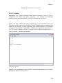
2.4.1.3 View Menu
View menu items control how the workflow appears on the Workflow canvas. Zoom
items are also available via the Toolbar.
Zoom Reset (Ctrl+Equals): Reset the view of the Workflow canvas to the default
settings.
Zoom In (Ctrl+Shift+Equals): Magnify the Workflow canvas for a more close-up
view. Kepler provides fixed levels of zoom.
Zoom Out (Ctrl+Minus): Pull back for a more distant view of the Workflow canvas.
Kepler provides fixed levels of zoom.
Zoom Fit (Ctrl+Shift+Minus): Display the current workflow in its entirety on the
Workflow canvas.
Automate Layout (Ctrl+T): Make a workflow more readable by automatically
configuring actor locations.
XML View: View the current workflow in XML mode. The workflow MoML XML will
be displayed in a viewing window.
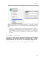
2.4.1.4 Workflow
Workflow menu items are used to run and modify open workflows.
Runtime Window: The Runtime Window command opens a Run window, which
allows users to adjust workflow parameters and run, pause, resume, or stop
workflow execution. Workflow results are displayed in the window as well.
Add Relation: Add a Relation to the Workflow canvas. Relations, which might also
be called “connectors”, allow actors to "branch" output to multiple places. For more
information about Relations, see Section 3.2.7.
Add Port: Add a port to the Workflow canvas. Select Input, Output, Input/Output,
Input Multiport, Output Multiport, or Input/Output Multiport. For more information
about ports, see Section 3.2.4.
Chapter 2
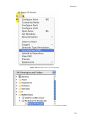
2.4.1.5 Tools
The Tools menu contains a number of useful tools that are used to build and
troubleshoot workflows.
Animate at Runtime: Select this menu item to highlight the actor that is currently
processing as the workflow is run. The active actors will be denoted with a red
highlight. Note: This command is only relevant when an SDF Director is used.
Listen to Director: Open a viewing window that displays the Director's activity,
noting when each actor is preinitialized, initialized, prefired, iterated, and wrapped
up.
Create Composite Actor: Create a new composite actor on the Workflow canvas.
For more information about composite actors, please see Section 3.2.3.
Expression Evaluator: Open an Expression Evaluation window used to evaluate
any Kepler expression. For more information about the expression language, see the
Ptolemy documentation.
Instantiate Component: Open the designated component on the Workflow canvas.
Components can be identified via class name (e.g., ptolemy.actor.lib.Ramp) or via a
URL. Use this menu command to easily access components that are not included in
the Kepler component tree (e.g., the DDF Director or Ptolemy actors that are not
included in the default Kepler library).
Instantiate Attribute: Open the designated attribute on the Workflow canvas.
Attributes
are
identified
by
class
name
(e.g.,
ptolemy.vergil.kernel.attributes.EllipseAttribute).
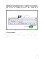
Check System Settings: Open a window containing system settings.
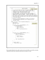
Ecogrid Authentication: Provide log in credentials or log out after using
features in Kepler that require authentication (e.g., an authenticated data search for
the KNB (Earthgrid) or uploading actors to the Kepler actor library).
Preferences: Set various Kepler preferences, including local and remote directories
used to find components for the component library and services used for data
sources.
Text Editor: Open a simple text editor used to create, edit, and save text files.
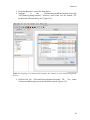
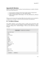
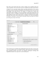
Module Manager: View modules in the current suite, load and save module
configurations, view downloaded modules, and view available modules, and switch
Chapter 2
to a different module configuration. For more information on the module manager,
see Chapter 12.
JVM Memory Settings: Adjust how much memory is allocated to Kepler. If your
computer has available RAM, you may want to allocate more memory to Kepler by
increasing the Max Memory setting. This may improve performance.
2.4.1.6 Window
Access the Runtime Window via the menu option.
2.4.1.7 Help
The Help menu contains information about the current version of Kepler as well as
links to useful help documentation.
About: Open a window containing the current Kepler version number.
Kepler Documentation: An index of useful Kepler documents.
Modules Documentation: An index of documentation for the installed modules.
2.4.2 Toolbar
The Kepler Toolbar contains the most commonly used Kepler functions (Figure 2.2).
The Toolbar can be dragged and dropped to a convenient screen location. Closing
the Toolbar returns it to the default position beneath the Menu bar and above the
Workflow canvas.
The Toolbar consists of three main sections: View, Run, and Ports, discussed in more
detail below.
Figure 2.2: The Kepler Toolbar.
Chapter 2
2.4.2.1 View Tools
View tools (Table 2.1) are used to zoom in, reset, fit, and zoom out of the workflow
on the Workflow canvas:
Zoom In: Magnify the Workflow canvas for a more close-up view. Kepler
provides fixed levels of zoom.
Zoom Reset: Reset the view of the Workflow canvas to the default
settings.
Zoom Fit: Display the current workflow in its entirety on the Workflow
canvas.
Zoom Out: Pull back for a more distant view of the Workflow canvas.
Kepler provides fixed levels of zoom.
Table 2.1 View tools
2.4.2.2 Run Tools
Run tools (Table 2.2) are used to run, pause, and stop the workflow.
Run: Run the workflow. The button will have an orange highlight when
the workflow is running.
Pause: Pause the workflow. The button will have an orange highlight
when the workflow is paused. To resume the workflow, click the Run
button.
Stop: Stops workflow execution. The button will have an orange
highlight when the workflow is stopped To restart the workflow, click
the Run button.
Table 2.2: Run tools
2.4.2.3 Port Tools
Port tools (Table 2.3) are used to add Relations or Ports to workflows:
Chapter 2
Input Port: Add a single input port. A single input port can be
connected to only a single channel of data. Single ports are designated
with a dark triangle on the Workflow canvas.
Output Port: Add a single output port. A single output port can emit
only a single channel of data. Single ports are designated with a dark
triangle on the Workflow canvas
Input/Output Port: Add a bi-directional port, which can receive or send
a single channel of data.
Multiple Input Port: Add a multiple input port. A multiple input port
can be connected to multiple channels of data. Multiple ports are
designated with a hollow triangle on the Workflow canvas.
Multiple Output Port: Add a multiple output port. A multiple output
port can emit multiple channels of data. Multiple ports are designated
with a hollow triangle on the Workflow canvas.
Multiple Input/Output Port: Add a multiple input/output port. A
multiple input/output port can receive or send multiple channels of
data. Multiple ports are designated with a hollow triangle on the
Workflow canvas.
Relation: Add a Relation. Relations “branch” a data flow so that data can
be sent to multiple places in the workflow.
Table 2.3: Port tools
2.4.3 Components, Data Access, and Outline Areas
The Components and Data Access area contains a library of workflow components
(e.g., directors and actors, under the Components tab) and a search mechanism for
locating those components, as well as data sets (under the Data tab). The Outline
area displays an outline tree of the components that are being used in the current
workflow. When the application is first opened, the Components tab is displayed.
2.4.3.1 Components Tab
Kepler comes standard with over 350 components that are stored on the local
machine and can be used to create an innumerable number of workflows with a
variety of analytic functions. The default set of Kepler processing components is
displayed under the Components tab in the Components and Data Access area. Users
can easily add new components or modify existing components as well. See Chapter
5 for more information about adding components to the local library.
Chapter 2
Components in Kepler are arranged in three high-level categorizations:
Components, Projects, and Statistics (Table 2.4). Any given component can be
classified in multiple categories, appearing in multiple places in the component tree.
Category
Components
Description
Contains a standard library of all components,
arranged by function.
Contains a
library of project-specific
components (e.g., SEEK or CIPRes)
Contains a library of components for use with
statistical analysis.
Projects
Statistics
Table 2.4: Component Categories in Kepler
Browse for components by clicking through the component trees, or use the search
function at the top of the Components tab to find a specific component.
To search for components:
1. In the Components and Data Access area to the left of the Workflow canvas,
select the Components tab.
2. Type in the desired search string (e.g., “File Reader”).
3. Click the Search button. The search results are displayed in the Components
and Data Access area, replacing the default list of components. You may
notice multiple instances of the same component. Because components are
arranged by category, the same component may appear in multiple places in
the search results.
4. To use one or more components in a workflow, simply drag the desired
components to the Workflow canvas.
5. To clear the search results and re-display the complete component library,
click the Cancel button.
NOTE: If you know the name of a component and its location in the Component
library, you can navigate to it directly, and then drag it to the Workflow canvas.
2.4.3.2 Data Tab
Via its search capabilities, Kepler provides access to data stored remotely on the
EarthGrid, which contains a wide collection of ecological and geographical
resources. Select the Data Tab (Figure 2.3) in the Components and Data Access area
to find and retrieve remote data sets.
Chapter 2
Figure 2.3: The Data Tab. A search has been performed to locate "Datos Meteorologicos", a data set stored
on the EarthGrid.
To search for data on the EarthGrid through Kepler:
1. In the Components and Data Access area, select the Data tab.
2. Click the Sources button and select the services to search (deselecting
unnecessary sources decreases search time).
3. Type in the desired search string (e.g., Datos Meteorologicos). Make sure that
the search string is spelled correctly. (You can also enter just part of the
entire string – e.g., ‘Datos’). If the search requires authentication (e.g.,
searches on the KNB Authenticated Query source), use the Tools > Ecogrid
Authentication menu option to specify credentials.
4. Click the Search button. The search may take several moments. When the
search is complete, a list of search results (i.e., Data actors) will be displayed
in the Components and Data Access area.
5. To use one or more data actors in a workflow, simply drag the desired actors
to the Workflow canvas.
When a data set is dragged from the Data tab to the Workflow canvas, Kepler
downloads the data from the remote source and stores it in the Kepler cache where
it can be accessed by the workflow or easily previewed. The cache (i.e.., the
Chapter 2
'.kepler' directory) is in the user's HOME directory, which is the default working
directory whenever one first opens a Command Window (on Windows platforms)
or a terminal window (on Mac or Linux). On Mac and Linux systems, the command
'cd ~' will change directories to the home directory. Once data is stored in the
cache, Kepler will automatically access the local copy rather than re-download the
data. If you would prefer to re-download the data, and you are using an
EML2Dataset actor, select the Check for latest version parameter to
override the default behavior. See Chapter 6 for more information.
.
Information about downloaded data can be revealed in three ways: (1) on the
Workflow canvas, roll over the Data actor’s output ports to reveal a tool tip
containing the name and type of data or (2) right-click the Data actor and select Get
Metadata to open a window that contains more information about the data set
(Figure 2.4) or (3) preview the data set by right-clicking the data actor and selecting
Preview from the drop-down menu (Figure 2.6).
Figure 2.4: Metadata for the Datos Meteorologicos data set.
Chapter 2
Figure 2.5: Previewing a data set.
Downloaded data can be output in a variety of formats. See Chapter 6 for more
information.
The EarthGrid currently interfaces with KNB Metacat database. The Knowledge
Network for Biocomplexity (KNB) is a national network intended to facilitate
ecological and environmental research on biocomplexity. It enables the efficient
discovery, access, interpretation, integration, and analysis of many kinds of
ecological data from a highly distributed set of field stations, laboratories, research
sites, and individual researchers. 9
To configure a data search to search a subset of the EarthGrid, click the Sources
button from the Data tab. Select the sources to be searched and the type of
documents to be retrieved (Figure 2.6) Each service requires that at least one
corresponding document type is selected (e.g., the KNB Metacat EcoGrid
QueryInterface service requires that either Ecological Metadata Language 2.0.0,
2.0.1, or 2.1.0 is selected). If you try to 'deselect' all of the relevant document types,
the service is automatically deselected as well. The document types (e.g., Ecological
9
Knowledge Network for Biocomplexity (KNB) website, http://knb.ecoinformatics.org
Chapter 2
Metadata Language 2.0.0) refer to the metadata specification used by the data sets.
For more information about metadata, please see Chapter 6.
Figure 2.6: Configuring the data sources and types.
2.4.4 Workflow Canvas
Scientific workflows are opened, created, and modified on the Workflow canvas.
Components are easily dragged and dropped from the Component and Data Access
area to the desired canvas location, and can then be dragged around on the canvas.
Each component is represented by an icon, which makes identifying the components
simple. Connections between the components (i.e., channels) are also represented
visually so that the flow of data and processing is clear.
Each time you open an existing workflow or create a new workflow, a new
application window opens. Multiple windows allow you to work on several
workflows simultaneously and compare, copy, and paste components between
Workflow canvases.
2.4.4.1 Director Right-Click Menu
The director right-click menu contains several menu items that are specific to the
director: Configure Director and Documentation.
Configure Director: Configure the director parameters. This dialog can also be
opened by double-clicking the director on the Workflow canvas.
Chapter 2
Documentation: Display, customize, or remove director
Customized documentation will replace existing documentation.
documentation.
2.4.4.2 Actor Right-Click Menu
The actor right-click menu contains several menu items that are specific to that
actor: Configure Actor, Customize Name, Configure Ports, Configure Units, Open
Actor, Get Metadata, Documentation, Listen to Actor, Suggest, Semantic Type
Annotation, Save in Library…, Save Archive (KAR)…, and Upload to Repository.
Configure Actor (Ctrl+E): Configure the actor parameters. This dialog can also be
opened by double-clicking the actor on the Workflow canvas.
Customize Name: Customize the label that identifies the actor on the Workflow
canvas.
Configure Ports: Add, remove, hide, show, rename, and customize input and output
ports.
Configure Units: Specify unit constraints for an actor (e.g., $plus=$minus, which
states that an actor's plus and minus ports must have the same units. For more
information,
please
see
the
Ptolemy
documentation,
http://ptolemy.berkeley.edu/ptolemyii/ptIIlatest/ptII/ptolemy/data/unit/demo/S
taticUnits/NonAppletStaticUnits.htm
Open Actor (Ctrl+L): Display the actor's Java source code in a viewing window.
Get Metadata: Display a data set's metadata. (For data actors only.)
Documentation: Display, customize, or remove director documentation.
Customized documentation will replace existing documentation on the local copy of
the actor in the current Kepler version. Note that customized documentation will
not be "transferred" if a new version of Kepler is installed.
Listen to Actor: Open a window that displays various actor events during
execution.
Suggest: Request that the semantic system suggest compatible input, output, or
similar components.
Semantic Type Annotation: Semantic annotations conceptually describe an actor
and/or its "data schema." Annotations provide the means for ontology-based
discovery and integration. Annotations are stored within the component metadata.
Chapter 2
Each port can be annotated with multiple classes from multiple ontologies.
Annotations can be used to find similar components, and to check that workflows
are semantically and structurally well typed.
Save Archive (KAR): Save an archived version of the selected component to a
selected location on the local machine.
Upload to Repository: Upload a component to the Kepler repository, which is a
centralized server where workflow components can be searched and re-used.
Uploaded components should have a unique name. To change the name of a
component, right-click it and select Customize Name from the drop-down menu.
Users will be prompted for a Knowledge Network for Biocomplexity (KNB) user
name and password; if you do not have a KNB user account, click the Login
Anonymously button to upload components without a user name or password.
Alternatively, you can register for a KNB account on the KNB homepage
(knb.ecoinformatics.org).
View LSID: View the unique life sciences identifier for this actor.
Preview: Display a data table. This option is only used by data actors (e.g.,
EML2Dataset) to display data sets represented by Meta data. For more information
about using data sets in Kepler, please see Chapter 6 of the User Manual.
2.4.5 Navigation Area
The navigation area contains a view of the entire workflow (even if only a portion of
the workflow is displayed on the Workflow canvas). Use the red guidelines to
navigate a large workflow and select a portion of the workflow to display (Figure
2.7)
Chapter 2
Figure 2.7: The Navigation are
Section 3
3. Scientific Workflows
Kepler simplifies the effort required to analyze and model scientific data by using a
visual representation of these processes. These representations, or “scientific
workflows,” display the flow of data among discrete analysis and modeling
components (Figure 3.1).
Figure 3.1: A simple scientific workflow developed in Kepler
Kepler allows scientists to create their own executable scientific workflows by
simply dragging and dropping components onto a workflow creation area and
connecting the components to construct a specific data flow, creating a visual model
of the analytical portion of their research. Kepler represents the overall workflow
visually so that it is easy to understand how data flow from one component to
another. The resulting workflow can be saved in a text format, emailed to
colleagues, and/or published for sharing with colleagues worldwide.
Kepler users with little background in computer science can create workflows with
standard components, or modify existing workflows to suit their needs. Quantitative
analysts can use the visual interface to create and share R and other statistical
analyses. Users need not know how to program in R in order to take advantage of its
powerful analytical features; pre-programmed Kepler components can simply be
dragged into a visually represented workflow. Even advanced users will find that
44
Section 3
Kepler offers many advantages, particularly when it comes to presenting complex
programs and analyses in a comprehensible and easily shared way.
Kepler includes distributed computing technologies that allow scientists to share
their data and workflows with other scientists and to use data and analytical
workflows from others around the world. Kepler also provides access to a
continually expanding, geographically distributed set of data repositories,
computing resources, and workflow libraries (e.g., ecological data from field
stations, specimen data from museum collections, data from the geosciences, etc.).
3.1 What is a Scientific Workflow?
Scientific workflows are a flexible tool for accessing scientific data (streaming
sensor data, medical and satellite images, simulation output, observational data,
etc.) and executing complex analysis on the retrieved data.
Each workflow consists of analytical steps that may involve database access and
querying, data analysis and mining, and intensive computations performed on high
performance cluster computers. Each workflow step is represented by an “actor,” a
processing component that can be dragged and dropped into a workflow via
Kepler’s visual interface. Connected actors (and a few other components that we’ll
discuss in later sections) form a workflow, allowing scientists to inspect and display
data on the fly as it is computed, make parameter changes as necessary, and re-run
and reproduce experimental results.10
Workflows can represent theoretical models or observational analyses; they can be
simple and linear, or complex and non-linear. One feature of some scientific
workflow systems is that they can be nested (i.e., hierarchical), meaning that a
workflow can contain “sub-workflows” that perform embedded tasks. A nested
workflow (known in Kepler as a composite actor) is a re-usable component that
performs a potentially complex task.
Scientific workflows in Kepler provide access to the benefits of today’s grid
technologies (providing access to distributed resources such as data and
computational services), while hiding the underlying complexity of these
technologies. Kepler automates low-level data processing tasks so that scientists can
focus instead on the scientific questions of interest.
Workflows also provide the following:


documentation of all aspects of an analysis
visual representation of analytical steps
10
Ludäscher, B., I. Altintas, C. Berkley, D. Higgins, E. Jaeger-Frank, M. Jones, E. Lee, J. Tao, Y. Zhao.
2005. Scientific Workflow Management and the Kepler System, DOI: 10.1002/cpe.994
45
Section 3



ability to work across multiple operating systems
reproducibility of a given project with little effort
reuse of part or all of a workflow in a different project
To date, most scientific workflows have involved a variety of software programs and
sophisticated programming languages. Traditionally, scientists have used STELLA or
Simulink to model systems graphically, and R or MATLAB to perform statistical
analyses. Some users perform calculations in Excel, which is user-friendly, but offers
no record of what steps have been executed. Kepler combines the advantages of all
of these programs, permitting users to model, analyze, and display data in one easyto-use interface.
Kepler builds upon the open-source Ptolemy II visual modeling system
(http://ptolemy.eecs.berkeley.edu/ptolemyII/), creating a single work environment
for scientists. The result is a user-friendly program that allows scientists to create
their own scientific workflows without having to integrate several different
software programs or enlist the assistance of computer programmers.
A number of ready-to-use components come standard with Kepler, including
generic mathematical, statistical, and signal processing components and
components for data input, manipulation, and display. R- or MATLAB-based
statistical analysis, image processing, and GIS functionality are available through
direct links to these external packages. You can also create new components or
wrap existing components from other programs (e.g., C programs) for use within
Kepler.
3.2 Components of a Workflow
Scientific workflows consist of customizable components—directors, actors, and
parameters—as well as relations and ports, which facilitate communication
between the components. Figure 3.2 displays a Kepler workflow with the main
workflow components identified.
The workflow in Figure 3.2, the LotkaVolterraPredatorPrey workflow, is used to
model the relative populations of a predator and its prey over time. For a more
detailed look at how it works, please see Section 4.2.3.
46
Section 3
Figure 3.2: Main window of Kepler with some of the major workflow components highlighted. The
windows on the bottom right are output windows, created by the workflow to display result graphs.
3.2.1 Directors
Kepler uses a director/actor metaphor to visually represent the various components
of a workflow. A director controls (or directs) the execution of a workflow, just as a
film director oversees a cast and crew. The actors take their execution instructions
from the director. In other words, actors specify what processing occurs while the
director specifies when it occurs.
Every workflow must have a director that controls the execution of the workflow
using a particular model of computation. For example, workflow execution can be
synchronous, with processing occurring one component at a time in a pre-calculated
sequence (SDF Director). Alternatively, workflow components can execute in
47
Section 3
parallel, with one or more components running simultaneously (which might be the
case with a PN Director).
A small set of commonly used directors come packaged with Kepler (Table 3.1), but
more are available in the underlying Ptolemy II software that can be accessed as
needed. For a more detailed discussion of workflow models of computation, please
see Section 5.2 Choosing a Director, or refer to the Ptolemy II documentation.
The SDF Director is often used to oversee fairly
simple, sequential workflows. Types of workflows
that run well under an SDF Director include
processing and reformatting data, converting one
data type to another, and reading and plotting a
series of data points.
The PN Director is often used for managing
workflows that require parallel processing on
distributed computing systems.
The Continuous Director is for the “continuous time”
domain, a timed domain that supports continuoustime signals, discrete-event signals, and mixtures of
the two. There is a global notion of time that all the
actors are aware of.
The DE Director is often used for modeling timeoriented systems: queuing systems, communication
networks, and occurrence rates or wait times.
The DDF Director is often used for workflows that
use looping or branching or other control structures,
but that do not require parallel processing (in which
case a PN Director should be used).
Table 3.1: Directors that come in the standard Kepler component library.
3.2.2 Actors
48
Section 3
Actors are the basic building blocks of workflows. Kepler comes packaged with
more than 530 actors, each ready to be used in new and/or existing scientific
workflows. Each actor is designed to perform a specific task: from generating
summary statistics, to mapping data points to a projection of North America, to
translating files from one format to another. Each actor performs a "step" in a
workflow. For example, one actor might be used to read or import data for use in a
workflow, another to transform that data into a format that can be analyzed,
another to analyze or graph the data, and another to output the data to a file or the
screen. Data passes between these actors via channels, which are represented by
solid lines on the Workflow canvas.
The actors are listed in the Components tab of the Kepler interface. Dragging and
dropping an actor will move it to the Workflow canvas, where it can be incorporated
into a workflow. However, simply dragging an actor onto the Workflow canvas will,
by itself, do nothing. Though each actor knows "what" processing should occur, it
does not know "when" to perform that process (or "iterate"). Actors need to be
directed (i.e., they require a Director component) in order to perform.
Separating the "what" from the "when" in actor performance allows actors to act
and interact in many ways. For example, an actor can be instructed to iterate once,
or ten times, or infinitely with a simple Director setting. Similarly, an actor can be
instructed to work in parallel with other actors—which is useful when workflows
require parallel processing on distributed computing systems—or at discrete times
along a time line, or in a number of other ways dictated by the Director. See Section
5.2 for more information about each Director and how to choose the right director
for each workflow.
New actors can be downloaded from the Kepler repository, or created by the user
and added to the Kepler application. User-created actors can also be uploaded to the
Kepler repository, where they can be shared with other workflow developers. The
Kepler repository is covered in more detail in Section 4.5.3. For more information
about creating and using new actors, see the appendix on Creating New Actors.
Kepler actors come in two forms: "individual" actors and "composite" ones.
Composite actors are collections or sets of individual actors bundled together to
perform more complex operations. Composite actors can be used in workflows,
essentially acting as a nested or sub-workflow (Figure 3.3). An entire workflow can
be represented as a composite actor and included as a component within an
encapsulating workflow. Composite actors are designated with a double rectangle
actor icon.
49
Section 3
Figure 3.3: Representation of a nested workflow. "B" is an example of a composite actor, which contains
three nested actors (D, E, and F).
Both individual and composite actors are identified by an icon and a label, which are
rendered on the Workflow canvas. In addition, most actors have one or more ports,
which are used either to input values (a dataset to analyze, for example) or to output
results. Most actors have parameters, as well, which are customizable settings. To
view and/or edit an actor's parameters, double-click the actor icon on the Workflow
canvas.
Figure 3.4 shows a Round actor as it appears on the Workflow canvas. The Round
actor has two ports, an input and an output port, as well as one parameter
(function). Double-click the actor to view and/or edit the function parameter.
Figure 3.4: The Round actor as it appears on the Workflow canvas
Actor Name: The actor name can be customized to specifically identify an actor's
function in a workflow. For example, a Display actor can be renamed "Display
Statistics" or "Display Errors" to better identify its purpose in a specific workflow.
To edit an actor name, right-click the actor icon from the Workflow canvas and
50
Section 3
select Customize Name from the menu. The actor name is displayed above the actor
icon unless the "Show name" option in the Customize Name menu is deselected.
Icon: Each actor is identified by an icon that describes the actor on the Workflow
canvas. Icons help identify the function of each actor. For a complete list of actor
icons and a description of Kepler actor symbology, see Section 5.3.1 Actor Icon
Families.
Ports: Most actors have one or more ports, depicted with either a white (multiport)
or black (single port) triangle at the perimeter of the actor icon. Data flows into and
out of the actor via these ports. To add, remove, or rename actor ports, right-click
the actor icon and select Configure Ports from the menu. Checking "Show Name"
displays the port name on the Workflow canvas.
Data is passed to actor ports in the form of tokens. A token can be thought of as a
container of some kind of data. Each token has a type ("integer" or "matrix," for
example), and this type is usually declared by the port that accepts or broadcasts the
data. Mouse over an actor port on the Workflow canvas to display a tooltip that
contains the port name as well as the type of data it produces or accepts. If the actor
does not receive data tokens of the specified type, an error will be generated.
Parameters: Double-click an actor icon on the Workflow canvas to reveal the
actor's parameters, or settings. Parameters are used to give actors context-specific
instructions, such as the location of a source file to read, a particular algorithm to
perform, and the format in which to output results.
Each time an actor is dragged onto the Workflow canvas from the Components tab, a
new "instance" of that actor is created. Dragging and dropping an ImageJ actor onto
the canvas three times will produce three instances of the ImageJ actor, named
ImageJ, ImageJ2, and ImageJ3. Editing the parameters of any one of these instances
does not affect the values of the other instances, nor does it affect the original actor
stored in Kepler. In other words, every time an actor is instantiated, it will have the
same settings as the original actor (or "class", in Java). The name of each actor class
can be viewed by right-clicking an actor and selecting Documentation from the
drop-down menu. The class name is displayed in parenthesis beside the actor name,
e.g., ImageJActor (Instance of util.ImageJActor).
Documentation: All Kepler actors have documentation, which can be opened via
the actor's right-click menu. To read the actor documentation, drag an actor onto
the Workflow canvas, right-click the actor icon, and select Documentation > Display
from the pop-up menu (Figure 3.5). Documentation can also be accessed from the
Components tab: simply right click an actor and select View Documentation. The
documentation describes each actor and its function, the type of values the actor
inputs and outputs, and the purpose of each actor parameter.
51
Section 3
Figure 3.5: Actor documentation
The actor documentation can also be customized by right-clicking the actor and
selecting Documentation > Customize from the drop-down menu. An editing
window opens (Figure 3.6).
52
Section 3
Figure 3.6 Editing actor documentation.
Documentation content can include links to external web pages (which will open in
a Kepler viewing window) and HTML formatting (<b>, <tt>, <li>, etc). XML-reserved
characters (e.g., '>', '&', '"', etc) must be escaped. The most common reserved
characters and their entity replacement are listed in Table 3.2
XML-reserved Character
&
<
>
"
'
Replace with:
&amp;
&lt;
&gt;
&quot;
&apos;
Table 3.2: Common XML-reserved characters.
To delete the content of a documentation screen, select Documentation > Remove
Customization. Note that this action cannot be undone with the "Undo" Menu bar item.
Actors make it easy to "read" the architecture of a workflow. When an existing
workflow is opened (or a new workflow is created), each actor appears on the
Workflow canvas, allowing users to easily follow the workings of the process that
the workflow performs.
Users can delve even deeper into the details of workflow processing by opening the
actors. To open an actor, right-click the actor icon from the Workflow canvas and
select Open Actor. For most individual actors, Kepler will display the Java source
code (Figure 3.7). The Java source is the code that creates the actor; some actors,
such as the RExpression actor, contain code (e.g., R-scripts), but this type of code is
accessed via actor parameters. In some cases, like the EML2Dataset actor, a
customized display of information about the actor appears when the actor is
53
Section 3
opened. If the actor is a composite actor, a new application window opens to display
the sub-workflow (Figure 3.8).
Figure 3.7: Viewing the source code for an individual actor. To open the source code in a viewing window,
right-click an actor and select Open Actor from the drop-down menu.
54
Section 3
Figure 3.8: Opening a composite actor. To view the nested (i.e., "sub-workflow") contained in a composite
actor, right-click the actor and select Open Actor from the drop-down menu.
Actors are written in Java, which is an object-oriented programming language
created by Sun Microsystems. (Note that existing code written in languages other
than Java can be included in Kepler by writing a Java "wrapper" around the code). A
technical specification of actor structure is beyond the scope of this manual, which
instead focuses on how actors are used and appear in the user interface. For more
technical information about actor code and coding practices, please see the Ptolemy
documentation as well as the Kepler developer documentation.
3.2.3 Composite Actors
Composite actors are collections or sets of actors bundled together to perform more
complex operations. Composite actors can be used in workflows, essentially acting
as a nested or sub-workflow. An entire workflow can be represented as a composite
actor and included as a component within an encapsulating workflow. In more
complex workflows, it is possible to have different directors at different levels. A
sub-workflow that contains its own director is called an opaque composite.
Transparent composites "inherit" their director from the containing workflow (i.e.,
the sub-workflow does not contain its own director).
55
Section 3
Opaque Composite actors are sub-workflows that contain their own director.
Opaque composite actors can be nested inside workflows that use a different type of
director, thereby combining different models of computation in one workflow;
however, not all directors are compatible. An opaque composite actor that uses a PN
director cannot be nested inside a workflow governed by an SDF director, for
example. For an in-depth discussion of directors that can be compatibly nested, see
Composing Models of Computation in Kepler/Ptolemy.
3.2.4 Ports
Each actor in a workflow can contain one or more ports used to consume or produce
data and communicate with other actors in the workflow. Actors are connected in a
workflow via their ports. The link that represents data flow between one actor port
and another actor port is called a channel. Ports are categorized into three types:



input port – for data consumed by the actor;
output port – for data produced by the actor; and
input/output port – for data both consumed and produced by the actor.
Each port is configured to be either a “singular” or “multiple” port. A single input
port can be connected to only a single channel, whereas a multiple input port can be
connected to multiple channels. As depicted in Figure 3.9, each single input port is
shown as black triangle, and each multiple port is shown as white triangle. A third
port color is grey, which means the port is port-parameter (please see Section
3.2.4.3: Port-Parameter). The "width" of the port describes how many channels of
data it accepts; the width of a single port can be 0 (unconnected) or 1, while the
width of a multiple port can be greater than 1. For multiple ports, the first channel is
number 0, the second 1, etc. See Section 3.2.5 for more information about channels.
Several different kinds of ports appear in Kepler: actor ports, external ports, and portparameters. Each is discussed in more detail in the following sections.
3.2.4.1 Actor Ports
Actor ports, also called coupled ports, are coupled with an actor. Actor ports appear
as light or dark triangles on the actor icons when actors are displayed on the
Workflow canvas (Figure 3.9), and can be customized by right-clicking an actor and
selecting Customize Ports from the drop-down menu.
56
Section 3
Figure 3.9: Single and multiple ports of the Bernoulli actor. A single port can be connected to a single
channel of data, while a multiple port can be connected to multiple channels.
To customize an actor's ports—either by changing the existing ports or adding new
ones--right-click the actor and select Configure Ports from the drop-down menu
(Figure 3.10)
Figure 3.10: Configuring the ports of the ConvertURLTo Image actor. Fields that cannot be edited are
noted with a pink highlight.
To add a new port, click the Add button and then customize the new port. Every port
must have a name, which can be customized by double-clicking the field in the Name
column and typing a name. In addition to selecting the kind of port (input, output or
input/output), users can assign a data type by clicking the Type field and selecting a
type from the drop-down menu. The port Direction field determines how the port
will be displayed on the Workflow canvas ("North" places the port at the top of the
actor, "South" on the bottom, etc). Kepler will display the port name on the
Workflow canvas if "Show Name" is selected, and will hide the port (i.e., not show it
on the Workflow canvas) if "Hide" is selected. Adding ports is essential to some
actors (like the Expression actor). In other cases, adding ports is relatively
meaningless since the actor is not designed to use any information on the added
port.
Units (seconds, meters, etc) can be selected by clicking the Units field and selecting a
measurement from the drop-down menu. Assigning units helps insure the integrity
of workflow processing (e.g., that meters are not added to miles per second, etc). If
units are assigned, the Unit Constraints Solver (accessed by right-clicking the
57
Section 3
Workflow canvas and selecting Unit Constraints Solver from the drop-down menu)
can be used to discover, analyze, and, in some cases, fix, unit inconsistencies that
exist in a model.
Each port can also be assigned a data type (e.g., double or array; See Section 3.2.6 for
more information about data types). The type of the port restricts the type of the
token that can pass through it. These types can be declared via the Type drop-down
menu, or left undeclared, in which case the application will resolve the type when
the workflow is executed. In many cases there is no need to enter port type
information.
3.2.4.1 External Port
An external port is often used to pass data from a sub-workflow to a containing workflow
(Figure 3.11). External ports can be connected by channels to other external ports or to
ports of individual actors.
Figure 3.11: Example of an external output port ("trigger") and an input port-parameter ("DirName"). This
simple workflow is a sub-workflow of the GARP_SingleSpecies_BestRuleSet-IV.xml workflow. The subworkflow passes a trigger to the containing workflow via its external trigger port. The DirName portparameter is discussed in greater detail in Section 3.2.4.3.
Like actor ports, external ports can be singular or multiple. They can be added to a
workflow with the Toolbar buttons. The ports are represented on the Workflow canvas
with the same icon that appears on the Toolbar buttons (Table 3.3)
58
Section 3
Icons for external ports
Single input port.
Multiple Input Port
Single output port.
Multiple Output Port
Single
Port
Input/Output
Multiple
Input/Output Port
Table 3.3: Icons that represent the various types of external ports on the Workflow canvas.
3.2.4.3 Port-Parameter
A port-parameter functions as both a port and a parameter that is used to configure the
operation of an actor (for more information about parameters, see Section 3.2.8). Portparameters allow users to specify a "default" value for a parameter (e.g., iterations=4 or
name="mouse"). If the actor receives a value via the coupled port, that value will replace
the value specified by the parameter component of the port-parameter.
Port-parameters can be added to workflows from the Components tab by searching for
"PortParameter" and dragging the component onto the Workflow canvas.
To customize a port-parameter on the Workflow canvas, right-click the portparameter and select Customize Name from the drop-down menu. A dialog window
provides a field for specifying a name (Figure 3.12). Choose a descriptive name and
click Commit.
Figure 3.12: Customizing the name of the port-parameter used in the GARP_SingleSpecies_BestRuleSetIV.xml workflow displayed in Figure 3.11.
Once the port-parameter has been named, specify a parameter value by double-clicking
the port-parameter (Figure 3.13).
59
Section 3
Figure 3.13: Customizing the parameter value of a port-parameter.
Note: The parameter value in Figure 3.13, DataDirectory+"/mephitis", in an
example of an expression, which is written in the Kepler expression language, and is the
value of the port-parameter used in the sub-workflow displayed in Figure 3.11.
DataDirectory is a parameter defined by the containing workflow, and
"/mephitis" is a string that will be concatenated to form the name of the new
directory created by the DirectoryMaker actor. Parameter values can also be constant
values, such as integers or strings.
Once the port-parameter has been defined, actors can reference it. Figure 3.14
displays the DirectoryMaker actor's parameters. Note that the value of the
"Directory name" parameter is set to $DirName. The "$" syntax is used to tell Kepler
to substitute the value of a string parameter for the parameter name (i.e., DirName
is the parameter name in this example, NOT the name of a directory). The value of
DirName is: DataDirectory+”/mephitis”. The actor will use this value unless
the port-parameter receives an alternate string from the containing workflow. In
the GARP workflow, the port-parameter is configured to receive
DataDirectory+"/"+SpeciesName (where SpeciesName is defined
elsewhere in the containing workflow), and this value would replace the default
Directory name parameter.
Figure 3.14: Referencing a port-parameter. The $DirName syntax is used to refer to the value of the
DirName port-parameter defined on the Workflow canvas.
3.2.5 Channels and Tokens
Channels are used to pass data from one port to another. Each channel can transport a
single stream of data. Data in Kepler is encapsulated and passed between workflow
components as tokens. Each token has an assigned data type (int, object, or matrix, for
example).
60
Section 3
Channels are represented as solid lines that "connect" the actors on the Workflow canvas.
To create a channel, left-click an actor's input or output port and drag the cursor to the
destination actor's input/output port. Until the channel is properly connected to both the
source and destination ports, the channel will appear as a thin black line. Once the
channel is connected, it will become a thick black line (Figure 3.15). To disconnect or
re-route one end of a channel, first select the channel by left-clicking somewhere along
the black line, then click-and-drag the appropriate end point to the desired location on the
Workflow canvas.
The simple addition/subtraction workflow displayed in Figure 3.15 contains two
channels of data that are input to an Add or Subtract actor via its multiport. The first
channel is number 0, the second number 1 (a third would be number 2, etc.).
Figure 3.15: Channels on the workflow canvas. When a channel is properly connected, it will be
represented by a thick black line. Channels that are not properly connected appear as thin black lines.
3.2.6 Data Types
Data tokens each have a structural type. "Hello", a string of alpha-numeric
characters, is encapsulated as a string token, while 3, an integer, is encapsulated as
an integer token. String and integer are both structural types.
A data token can only be passed to a port that accepts its structural type. An array of
strings cannot be passed to a port that accepts only integers, and attempting to do
so will generate a type error. Port data types are defined by the actor, and can be
configured by right-clicking an actor and selecting Configure Ports from the dropdown menu. That menu contains common Kepler data types, defined in Table 3.4.
Note that this list is not exhaustive. For example, users can edit the results from the
drop-down type menu to convert ‘ArrayType[int]’ to ‘ArrayType[double]’
Structural Data Types
Boolean
The Boolean token can have one of two values: true or
false (represented by 1 or 0, respectively).
61
Section 3
Complex
Double
Fixed point
General
Int
Long
Matrix
Object
Scalar
String
Unknown
A complex number consists of a real and imaginary
part. In Kepler, the imaginary component of a complex
number is designated with an i or j (e.g., 6+7i).
A double represents a floating point number (e.g., 1.345)
with "double precision". This data type can accurately
represent about twice as many significant digits as a single
precision type, but also requires more memory.
A fixed-point number is a number in which the position of
the decimal point is constant. U.S. currency can be
represented by a fixed-point number that has two digits to
the right of the decimal point, for example. Fixed point
numbers in Kepler are represented in the following way:
fix(value, integerBits, fractionBits).
The general data type is the most inclusive of the types. A
port assigned type "general" can accept data of all types
(array, string, matrix, etc.).
The integer token ("int") represents numerical values that
have no decimal points (e.g., 11 or -17)
Integers followed by an "l" or "L" are of type long. The
long data type can represent large integers. Float and
double data types can also be used: these data types have
greater storage capacity than long data types, but less
precision/significant digits.
A matrix contains boolean, complex, double, fixedpoint,
int, or long data that can be referenced by row and
column. Matrices in Kepler are specified with brackets.
Commas separate row elements and semicolons separate
rows. For example, a 1x3 matrix would be represented as
[1,2,3]. A 2x2 matrix would be represented by [1,2;3,4].
To create multidimensional matrices, use arrays of arrays
of arrays.
An object token is a data container for an arbitrary Java
object (most complex 'things' in Java are objects). These
tokens can be used to pass complex Java objects around a
Kepler workflow. Object tokens are primarily used for
custom workflows with custom actors. Non-programmers
will probably not find them very useful.
The term scalar designates a value that consists only of
magnitude (as opposed to a vector, which consists of both
a magnitude and direction). In Kepler, scalar values may
have any scalar data type: double, int, long, etc.
A sequence of characters specified within quotation
marks. Anything between "" is interpreted as a string.
An unknown data type places no additional type
constraints on the port. All the structured types are
less than the type "general" and greater than
62
Section 3
Unsigned byte
xml token
arrayType(int)
arrayType(int,5)
[Double]
{x=double, y=double}
"unknown."
An unsigned byte represents an integer that does not
include data to specify whether it is positive or negative.
Extensible Markup Language (XML) tokens use markup
language to describe the structure of the data. For more
information about XML, see the World Wide Web
Consortium.
An array is a data structure consisting of elements that can
be identified by a key (or index). The first item in an array
has a key of 0, the second 1, etc. Arrays in Kepler are
denoted
with
curly
braces,
e.g.
{1,2,3,4,5}
arrayType(int) specifies an array of integers. Note
that any type in the drop-down menu can be edited so that
different array types can be specified.
An array is a data structure consisting of elements that can
be identified by a key (or index). arrayType(int,5)
specifies an array of integers with 5 elements in the array
(i.e., the length of the array is specified as part of the type.
Note that any type in the drop-down menu can be edited
so that different array types and lengths can be specified.
A matrix with elements of type double.
A record token consists of named elements and their
values. In Kepler, records are specified between curly
braces. For example, {a=1, b=2} is a record with two
elements, named a and b, with values 1 and 2,
respectively. In this case, both values are of type double.
Table 3.4: Common data types in Kepler.
Kepler will attempt to automatically convert data into the appropriate structure. For
example, if an integer and a double are added, Kepler will determine that the result will
be type double (which is the "greater" of the two data types). For a detailed discussion
about type conversion and resolution see the Ptolemy documentation.
3.2.7 Relations
Relations allow workflows to “branch” a data flow. Branched data can be sent to
multiple places in the workflow. For example, a user might wish to direct the output
of an operational actor to another operational actor for further processing, and to a
display actor to display the data at that specific reference point. By placing a
Relation in the output data channel (Figure 3.16), the user can direct the information
to both places simultaneously.
63
Section 3
Figure 3.16: A relation is used to branch the Result output of the WebService actor to an XML Entry
Display actor and two additional processing components: Sequence Getter Using XPath and HTML
Generator Using XSLT.
To add a relation to a workflow, use the Add Relation button on the Toolbar (
). The relation will be placed in the center of the Workflow canvas. Drag and drop it
to the required location. When connecting a relation to actors, it is often easiest to
begin drawing the channel at the input or output port of the actor and connecting
the channel to the relation.
3.2.8 Parameters
Parameters are configurable values that can be attached to a workflow (model
parameters) or to individual directors or actors (coupled parameters). Actor
parameters specify everything from the directory into which the actor should save
its output, to the name applied to the output file, to the number of items the actor
should process. Director parameters control the number of workflow iterations and
the relevant criteria for each iteration. Model parameters define values that can be
adjusted in the Runtime window. More information about each type of parameter is
contained in the following sections.
3.2.8.1 Actor Parameters
Actor parameters (or "coupled parameters") are parameters that belong to an actor
or director. To view or edit these parameters, right-click the actor or director on the
Workflow canvas and select Configure Actor from the drop-down menu, or simply
double-click the component. This opens dialog box containing all of the relevant
64
Section 3
parameters. Figure 3.17 shows a dialog box that contains the parameters of the
Display actor.
Figure 3.17: Parameters of the Display actor.
To edit the parameter values, simply change the fields and click the Commit button.
In most cases, values must be modified before the workflow begins running; in other
words, changes to parameter values will not go into effect if the workflow is already
running.
Parameters can be added, removed, or restored to their default values via the
corresponding buttons. Click Preferences to customize the type of field used to edit
the parameters: text, fixed, line, or check box (Figure 3.18).
Figure 3.18: The Preferences button is used to manage the types of fields used to edit parameter values.
The pictured parameters are for the Bernoulli actor, which is used to generate and output a sequence of
random Boolean values.
65
Section 3
3.2.8.2 Model Parameters
Model parameters appear directly on the workflow canvas and are used to specify values
for anything from a color, to a file name, to a required version number (Figure 3.19).
Model parameters can be added to a workflow from the Components tab.
To customize the value of a model parameter, double-click the parameter on the
Workflow canvas, type a value into the editable field, and click OK. Alternatively, model
parameters can be adjusted in the Runtime window, which is accessed via the Workflow
menu.
Figure 3.19: Model parameters, which is set on the Workflow canvas. Model parameters can be referenced
by any actor in the workflow and its sub-workflows.
66
Section 3
Parameter values can be referenced by any actor in the workflow or its sub-workflows.
Actors reference model parameters by name. For example, the ClimateFileProcessor
actor in Figure 3.20 references the OutputDir model parameter in its
baseOutputFileName parameter.
Figure 3.20: Referencing a model parameter.
3.2.8.3 Port-Parameters
A port-parameter functions as both a port and a parameter that is used to configure the
operation of an actor. For more information about Port-Parameters, see Section 3.2.4.3.
67
Section 4
4. Working with Existing Scientific Workflows
Kepler comes with a set of documented workflows contained in the "demos"
directory and its subdirectories. The workflows in the "demos/getting-started"
directory are useful examples that can help users familiarize themselves with the
application, and many of the workflows contained in that directory are described in
more detail later in this chapter.
In this chapter, we also cover how to open workflows created and shared by
colleagues, and how to modify and save existing workflows.
4.1 Opening Workflows
Kepler can open both local workflows and workflows stored on a remote Web
server. In both cases, the open workflow will display on the Workflow canvas,
where it can be run and/or modified.
4.1.1 Opening Local Workflows
The
workflows
shipped
with
Kepler
are
installed
into
the
"KeplerData/workflows/module/Module-2.X.Y/demos/getting-started/" directory
(where Module is the name of each Kepler module and X.Y is the current version of
Kepler, and KeplerData/ is inside your Documents and Settings directory on
Windows, and your home directory on Linux and Mac). (In general, workflows can
be stored and opened from any local directory.)
To open an existing local XML (MoML) workflow:
1. From the Menu bar, select File, then Open… . A standard file dialog box will
appear.
2. If the file dialog box does not open to the “KeplerData” directory (the place
where user workflows and data are stored), then navigate to the
“KeplerData” directory (in your home directory).
3. Double-click a workflow file to open it (or single-click to select the file and
then click the Open button). The workflow will appear on the Workflow
canvas.
For example, to open the Lotka-Volterra workflow, the classic predator-prey model
that is shipped with the Kepler application:
68
Section 4
1. From the Menu bar, select File, then Open… .
2. Navigate
to
the
“KeplerData/workflows/module/outreach2.X.Y/demos/getting-started/" directory and locate the file named “02LotkaVolterraPredatorPrey.xml” (Figure 4.1).
Figure 4.1: Navigating to the Lotka-Volterra workflow. The workflow is in the “demos/getting-started"
directory.
3. Double-click the “02-LotkaVolterraPredatorPrey.xml” file.
The LotkaVolterra workflow appears on the Workflow canvas (Figure 4.2).
69
Section 4
Figure 4.2: The Lotka-Volterra workflow in the Kepler interface.
Since Kepler 2.4, the demo workflows in each Kepler module can be found in the
Kepler component tree. The ‘Demos’ folder in component tree lists all demo
workflows for each module. Users can search/navigate Kepler component tree to
find interested workflows and open them by double-clicking them.
4.2 Running Workflows
Workflows can be run in one of two ways: via the Run button in the Toolbar, or via
the Workflow menu's Runtime Window menu item.
4.2.1 Runtime Window
70
Section 4
Selecting the Runtime Window menu item (Figure 4.4) opens a handy window that
can be used to start, pause, resume, and stop workflow execution. The window also
displays all workflow and director parameters so that they can be viewed and/or
edited. Workflow output is displayed in the window once the workflow has
executed.
To run a workflow using the Runtime Window:
1. Open the desired workflow.
2. From the Menu bar, select Workflow, then Runtime Window. A Runtime
window opens. Workflow and director parameters are displayed on the left
side of the window, where they can be adjusted as needed.
3. Click the Go button to start running the workflow.
4. The workflow will execute. During workflow execution, you may select the
Pause, Resume, or Stop buttons.
Figure 4.3: Opening the Runtime Window to run a workflow and/or adjust workflow parameters. In this
example, the Runtime window is displaying the Lotka-Volterra workflow.
To run the Lotka-Volterra workflow via the Runtime Window:
1. Open the workflow file named “02-LotkaVolterraPredatorPrey” from the
“demos/getting-started/” directory.
71
Section 4
2. From the Menu bar, select Runtime Window from the Workflow menu. A
Runtime Window opens.
3. Click the Go button in the Runtime Window.
4. The Lotka-Volterra workflow will execute with the default parameters and
produce two graphs, which are displayed in the window. The graph labeled
TimedPlotter depicts the interaction of predator and prey over time (i.e., the
cyclical changes of the predator and prey populations over time predicted by
the model). The graph labeled XYPlotter depicts a phase portrait of the
population cycle (i.e., the predator population against the prey population).
Together these graphs show how the predator and prey populations are
linked: as prey increases, the number of predators increase. (Figure 4.5)
Figure 4.4: The Runtime Window displaying the results output by the Lotka-Volterra workflow.
4.2.2 Run Button
The Run button in the Toolbar runs a workflow with a single button click. Workflow
and director parameters are not exposed for editing as they are in the Runtime
Window.
To run a workflow using the Run Toolbar button:
1. Open the desired workflow.
72
Section 4
2. From the Toolbar, select the Run button. (
)
3. The workflow will execute and produce the specified output.
To run the Lotka-Volterra workflow via the Run button
5. Open the workflow file named “02-LotkaVolterraPredatorPrey” from the
“demos/getting-started/” directory.
6. On the Toolbar, click the Run button.
7. The Lotka-Volterra workflow will execute with the default parameters and
produce two graphs. The graph labeled TimedPlotter depicts the interaction
of predator and prey over time (i.e., the cyclical changes of the predator and
prey populations over time predicted by the model). The graph labeled
XYPlotter depicts a phase portrait of the population cycle (i.e., the predator
population against the prey population). Together these graphs show how
the predator and prey populations are linked: as prey increases, the number
of predators increase. (Figure 4.6)
73
Section 4
Figure 4.5: Graphs output by the Lotka-Volterra workflow run via the Run button on the Toolbar.
4.2.3 Running Workflows with Adjusted Parameters
Workflow parameters are used to specify anything from the name of a data
directory used by a workflow, to the relationship between items processed by the
workflow, to the name applied to a workflow's output file. Adjusting these
parameters can have a significant effect on the output.
Parameters can be adjusted in one of several ways. Double-click any workflow
parameters that appear on the Workflow canvas (e.g., r, a, b, or d in Figure 4.7) to
edit the parameter value. Director and actor parameters can be modified by doubleclicking the component and editing the values in the dialog window. If the workflow
is run via the Workflow menu's Runtime Window menu item, both workflow and
74
Section 4
director parameters are exposed and can be edited in the Runtime Window
interface before the workflow is run.
In this section, we will step through the process of adjusting the parameters of the
Lotka-Volterra workflow to show how adjusting parameters affects workflow
output.
Figure 4.6: The Lotka-Volterra workflow.
The Lotka-Volterra model was developed independently by Lotka (1925)11 and
Volterra (1926)12 and is made up of two differential equations. One equation
11
Lotka, Alfred J (1925). Elements of physical biology. Baltimore: Williams & Williams Co.
75
Section 4
describes how the prey population changes (dn1/dt = r*n1 - a*n1*n2), and the other
describes how the predator population changes (dn2/dt = -d*n2 + b*n1*n2).
The Lotka-Volterra model is based on certain assumptions:
 the prey has unlimited resources;
 the prey's only threat is the predator;
 the predator is a specialist (i.e., the predator's only food supply is the prey);
and
 the predator's growth depends on the prey it catches
The Lotka-Volterra model is represented in Kepler as a scientific workflow that
contains:
 six actors - two plotters, two equations, and two integral functions;
 one director; and
 four workflow parameters (Table 4.1).
NOTE: The director of the Lotka-Volterra model has several configurable
parameters as do the two plotter actors.
The critical assumptions above provide the basis for the workflow parameters. The
workflow parameters and their defaults are as follows:
Parameter
r
Default
Value
2
a
0.1
b
0.1
d
0.1
Description
The intrinsic rate of growth of prey in the
absence of predation
Capture efficiency of a predator or death rate of
prey due to predation
Proportion of consumed prey biomass
converted into predator biomass (i.e., efficiency
of turning prey into new predators)
Death rate of the predator
Table 4.1: Description of the default parameters for the Lotka-Volterra workflow
In the differential equations used in the workflow, (dn1/dt = r*n1 - a*n1*n2) and
(dn2/dt = -d*n2 + b*n1*n2), the variable n1 represents prey density, and the
variable n2 represents predator density.
When changing parameters in a workflow, the assumptions of the model must be
kept in mind. For example, if creating a Lotka-Volterra model with rabbits as prey
and foxes as predators, the following assumptions can be made with regard to how
the rabbit population changes in response to fox population behavior:
12
Volterra, Vito (1926) Fluctuations in the abundance of a species considered mathematically. Nature 118.
558-560.
76
Section 4





The rabbit population grows exponentially unless it is controlled by a
predator;
Rabbit mortality is determined by fox predation;
Foxes eat rabbits at a rate proportional to the number of encounters;
The fox population growth rate is determined by the number of rabbits they
eat and their efficiency of converting the eaten rabbits into new baby foxes;
and
Fox mortality is determined by natural processes.
If you think of each run of the model in terms of the rates at which these processes
would occur, then you can think of changing the parameters in terms of percent of
change over time.
To run the Lotka-Volterra workflow with adjusted parameters:
1. Open the workflow file named “02-LotkaVolterraPredatorPrey” from the
“demos/getting-started” directory
2. From the Menu bar, select Runtime Window from the Workflow menu. The
Runtime window opens. Notice there are two sets of parameters – one for the
workflow and one for the director. For more detail about the director
parameters, right-click the director and select Documentation > Display from
the drop-down menu. In this example, you will make adjustments to both
workflow and director parameters.
3. Adjust the workflow parameters as suggested in Table 4.2.
Parameter
r
New value
0.04
a
0.0005
b
0.1
d
0.2
Description
The intrinsic rate of growth of prey in the
absence of predation
Capture efficiency of a predator or death
rate of prey due to predation
Proportion of consumed prey biomass
converted into predator biomass (i.e.,
efficiency of turning prey into new
predators)
Death rate of the predator
Table 4.2: Description of the suggested parameters for the Lotka-Volterra workflow taken from
http://www.stolaf.edu/people/mckelvey/envision.dir/lotka-volt.html
4. Adjust the value of the stopTime director parameter to 300.
5. In the Runtime window, click the Go button.
The Lotka-Volterra workflow will execute with the adjusted parameters and
produce two graphs: 1) the TimedPlotter graph and 2) the XYPlotter graph. Note
77
Section 4
that with the changes in the parameters, the relationship between the predator and
prey populations are still linked but the relationship has changed (Figure 4.8).
Figure 4.7: Graphs output by the Lotka-Volterra model with adjusted parameters
4.3 Modifying Workflows
There are two basic ways to modify an existing scientific workflow:


Substitute a different data set for the current data set;
Substitute one or more analytical processes in the workflow with other
analytical processes (e.g., substitute a neural network model actor for a
probabilistic model actor).
In order to be substituted, data sets and processing components must be compatible
with the workflow. Workflow documentation should contain information about the
type of data and processing that occur in the workflow; if not, you may need to do
some investigative research: roll over actor ports to see the name of the port and the
type of data it accepts or broadcasts; right-click individual actors and select
Documentation to read more about the type of processing it does; or open existing
data files used by the workflow to see how they are formatted.
78
Section 4
The basic steps involved in modifying a workflow are:
1. Open the desired workflow.
2. Identify which workflow component is the target for substitution.
3. Select the target component (data actor or processing actor) by clicking it.
The selected component will be highlighted in a thick yellow border.
4. Press the Delete key on your keyboard. The highlighted component will
disappear from the Workflow canvas.
5. From the Components and Data Access area, drag an appropriate data or
processing actor to the Workflow canvas.
6. Connect the appropriate input and output ports and customize the actor
parameters
7. Run the workflow.
4.3.1 Substituting Data Sets
Substituting data sets involves "pointing" the workflow to a new set of data. For local
data, a data set is often specified by an Expression or a StringConstant actor, which use
an expression to generate the location of the data file (see Chapter 8 for more information
about the Expression actor). Other times, the location of the data set is specified as a
workflow or actor parameter. Remote data is often accessed via Kepler data actors that
handle all of the mechanical issues associated with parsing the Ecological Metadata
Language (EML) that describes the data, downloading the data from remote servers if
applicable, understanding the logical structure of the data, and emitting the data for
downstream actors to use when required.
In this section, we'll look at how to substitute a local data set into a workflow as well as
how to substitute remotely stored data sets that use EML. Before substituting data sets
into a workflow, you must ensure that the data are formatted as required by the workflow
(e.g., a tab-separated list or a table with metadata) and that the units and data types are
compatible.
Substituting a Local Data Set
Kepler can read data in many ways and from many formats. For example, the
workflow in Figure 4.9 uses a FileReader actor to access the contents of a data table
saved in a text format. A Display actor then displays the data in a text window.
79
Section 4
Figure 4.8: Using and displaying local data in a workflow.
The FileReader actor opens the local data file specified by the actor's parameters. To
substitute another file, simply double-click the FileReader actor to expose its
parameters, click the Browse button to the right of the actor's fileOrURL
parameter, and navigate to the desired file (Figure 4.10). Select a file and click the
Commit button. The actor is now configured to read the specified file.
Figure 4.9: Configuring the FileReader actor to use data from your local machine.
80
Section 4
NOTE: When creating a workflow, remember that the limitations of the data
determine which processing components are appropriate.
The ReadTable.xml workflow (Figure 4.11), which is included in the
KeplerData/workflows/module/r-2.X.Y/demos/R/ directory, is an example of a
workflow that reads a local text-based data file containing species occurrence data
("mollusc_abundance.txt"). The workflow extracts the species names from the data
set as well as the species count and creates a plot of the data (Figure 4.12). See
Chapter 8 for more information about R and how this workflow operates. For now,
we are only concerned with how the workflow accesses data, and how users can
substitute a new data set.
Figure 4.10: The ReadTable.xml workflow.
81
Section 4
Figure 4.11: Output of the ReadTable.xml workflow. The workflow extracts each species name and
occurrence information from the mollusc_abundance.txt data file, and creates a plot of the data.
The workflow uses an Expression actor labeled Data File Name to reference the data
set. The value:
property("r.workflowdir")+"demos/R/mollusc_abundance.txt"
is an expression written in the Kepler expression language. The expression
'property(“r.workflowdir”)' returns the path to the R module’s workflow
directory in KeplerData. "demos/R/mollusc_abundance.txt" is the rest of
the path to this data file.
In this workflow, the input file is a text file containing data in a 'spreadsheet-like'
tabular format. Each line of the file contains one row of values, separated by a
'separator' delimiter—a tab ("\t"), as specified by the workflow's Separator actor.
By default, the first row of the data file is assumed to contain the column names.
82
Section 4
(Setting the value of the header actor to FALSE will change this default). Saving an
Excel spreadsheet as a text file creates such a data file with a tab separator (Figure
4.13).
Figure 4.12: The mollusc_abundance.txt data set used by the ReadTable.xml workflow. Data is contained
in columns separated by a tab delimiter.
To use another set of data, simply ensure that the data are formatted correctly, and
substitute the name of the new data set into the Data File Name actor.
Substituting Remote Datasets Via the EarthGrid
Substituting data sets that are stored remotely on the EarthGrid is another simple way to
edit a workflow. For example, the workflow displayed in Figure 4.14 reads an
Intergovernmental Panel on Climate Change (IPCC) data set containing cloud cover data
that are stored on the EarthGrid. This dataset uses EML metadata to describe the data,
and can therefore be downloaded and accessed with the EML2Dataset actor (named
IPCC Climate Change Data: 1961-1990, Cloud Cover in the example workflow).
The workflow converts the data to a new format (see the documentation for the
ClimateFileProcessor actor for more information) and saves it.
83
Section 4
Figure 4.13: The example workflow processes an IPCC data set stored and accessed from the EarthGrid.
The data are described using Ecological Metadata Language (EML).
To use the workflow to convert other data (rainfall, wind, temperature, etc), simply
navigate to Kepler's Data tab and search for IPCC (Figure 4.15). Kepler will locate other
IPCC data sets, which will be displayed in the Data tab. Dragging and dropping any EML
data set onto the Workflow canvas instantiates an EML2Dataset actor, which downloads
the data so that it can be used by the workflow. The EML2Dataset actor will
automatically configure itself to provide one port for each attribute described by the EML
description. For example, if the data consist of four columns, the ports might be "Site",
"Date", "Plot", and "Rainfall."
84
Section 4
Figure 4.14: Searching for IPCC climate data sets stored on the EarthGrid.
The example workflow can be used to convert any historical IPCC data set. Future
climate change data require a ClimateChangeFileProcessor actor instead of the
ClimateFileProcessor actor.
Note that the EML2Dataset actor can be configured to output the data in one of a variety
of different formats. In the example, the EML2Dataset actor has been configured to
output data "As Cache File Name." To configure a data actor, double-click it and select
the appropriate data output format (Figure 4.16).
85
Section 4
Figure 4.15: Customizing the data output format of the data actor.
For more information about data output formats, please see Chapter 6.
4.3.2 Substituting Analytical Components
Kepler comes with hundreds of ready-to-use components that can be plugged into
existing workflows to customize the workflow processing. Data can be converted
into a variety of different formats or displayed in different ways. In this section, we
will look at how to change the way a workflow displays its output by substituting
one kind of display actor for another.
The Image Display workflow found under “demos/getting-started/03-ImageDisplay.xml”
(Figure 4.17) converts an image--a bitmapped image representing the species distribution
of the species Mephitis, a skunk, throughout North and South America—and then
displays the image using an ImageJ actor, which uses the ImageJ application to open and
work with a wide variety of images (tiffs, gifs, jpegs, etc.) For more information about
ImageJ, see Chapter 8.
Figure 4.16: The Image Display workflow. The ImageJ actor is highlighted.
86
Section 4
The Image Display workflow converts the specified image, a jpeg file, to a png
format and then displays it (Figure 4.18). The actor also opens the ImageJ
application, which can be used to modify the image via a handy toolbar (Figure
4.19).
Figure 4.17: The output of the ImageJ actor. The image was originally created by GARP, a genetic
algorithm that creates an ecological niche model for a species that represents the environmental conditions
where that species would be able to maintain populations. GARP was originally developed by David
Stockwell, at the San Diego Supercomputer Center. For more information on GARP, see
http://www.lifemapper.org/desktopgarp/.
Figure 4.18: The ImageJ toolbar that permits users to modify the image.
Rather than using ImageJ to display the workflow output, you may wish to use a
simple browser interface. To do so requires a single actor substitution—swapping a
BrowserDisplay actor for the ImageJ one. To make the substitution:
1. Open the 03-Image-Display.xml workflow from the “demos/getting-started/”
directory.
2. Select the target component, the ImageJ actor in this case. The ImageJ actor
will be highlighted in a thick yellow border, indicating that it is selected.
3. Press the Delete key on your keyboard. The ImageJ actor will disappear from
the Workflow canvas.
87
Section 4
4. From the Components and Data Access area, drag the Browser Display actor
to the Workflow canvas. You can find the Browser Display actor in the
Components tab under “Components > Data Output > Workflow Output >
Textual Output.”
5. Connect the output port of the ImageConverter actor to the input port of the
Browser Display actor. To connect the ports, left-click and hold the output
port (black triangle) on the right side of the Image Converter actor, drag the
pointer to the upper input port on the left side of the Browser Display actor,
and then release the mouse. If the connection is made, you will see a thick
black line (Figure 4.20). If the connection is not completely made, the line
will be thin.
6. Run the workflow. Note that the image is now displayed in a browser
window (Figure 4.21).
Figure 4.19: The Image Display workflow with the Browser Display actor substituted for the ImageJ actor.
NOTE: Sometimes the easiest way to connect actors is to go from the output port of
the source to the input port of the destination.
88
Section 4
Figure 4.20: The image displayed by the Browser Display actor.
4.4 Saving Workflows
Workflows are saved in KAR or XML format, which can be easily stored and shared.
To save a workflow, select the Save, Save As, or Export As… menu item from the File
menu, then name the file and select a save location.
For instructions on saving a workflow and sharing it with others, see Section 5.9
Saving and Sharing Workflows.
4.5 Searching for Data and Components
Kepler provides a searching mechanism to locate data (on the EarthGrid) and
analytical processing components (on the local system as well as the remote Kepler
repository).
4.5.1 Searching for Available Data
Via its search capabilities, Kepler provides access to data that is stored on the
EarthGrid. EarthGrid resources are stored in the KNB Metacat and the KU Digir
databases. For more information about the EarthGrid, see Chapter 2.
89
Section 4
To search for data on the EarthGrid:
1. In the Components and Data Access area, select the Data tab (Figure 4.22).
2. Type in the desired search string (e.g., Datos Meteorologicos). Make sure that
the search string is spelled correctly. You can also enter just part of the entire
string – e.g. ‘Datos’.
3. To configure the search, click the Sources button (make sure the Data tab is
selected). Selecting the sources to be searched and the type of documents to
be retrieved can help streamline the search and reduce the amount of time
required to return results. For example, because Datos Meteorologicos is
stored in the KNB Metacat database, the data source for the search can be
limited to just that node on the grid. In the Source dialog window, uncheck
“KNB Metacat Authenticated Query Interface" and click OK.
4. Click the Search button. Results may take 20 seconds to return. A status bar
at the bottom of the Data tab scrolls until the search is complete. When the
search is complete, a list of search results will be displayed in the
Components and Data Access area. The number of returned results is
displayed in the status area.
5. To use one or more data actors in a workflow, simply drag the desired data
set to the Workflow canvas.
90
Section 4
Figure 4.21: Searching for and locating Datos Meteorologicos, a data set that is stored on the EarthGrid.
For more information about the data set, right-click Datos Meteorologicos in the
Components and Data Access area or on the Workflow canvas and select Get
Metadata (Figure 4.23). Depending upon the amount of information entered by the
provider, much valuable metadata can be obtained. For example, the type of value
and measurement type of each attribute help you decide which statistical models
are appropriate to run.
91
Section 4
Figure 4.22: Viewing Metadata
The data actor will automatically configure its output ports to match the data.
Mouse over the data ports to reveal a port tooltip (Figure 4.24). The tooltip contains
the name of the port/data field as well as the data type.
Figure 4.23: Identifying data ports. Mouse-over each output port to reveal the port tooltip.
You can also preview the data set by right-clicking the actor and selecting Preview
from the drop-down menu (Figure 4.25).
92
Section 4
Figure 4.24: Previewing the Datos Meteorologicos data set.
4.5.2 Searching for Standard Components
Kepler comes standard with over 350 workflow components and the ability to
modify and create your own. Users can create an innumerable number of workflows
with a variety of analytic functions. The default set of Kepler processing
components is displayed under the Components tab in the Components and Data
Access area. Components are organized by function (e.g., “Director” or “Filter”). To
search for processing components:
1. In the Components and Data Access area to the left of the Workflow canvas,
select the Components tab.
2. Type in the desired search string (e.g., “File Reader”).
3. Click the Search button. When the search is complete, the search results are
displayed in the Components and Data Access area. The search results
93
Section 4
replace the default list of components. You may notice multiple instances of
the same component; this is because the same component may appear in
multiple categories in the search results.
4. To use one or more components in a workflow, simply drag the desired
components to the Workflow canvas.
5. To clear the search results and re-display the list of default components, click
the Cancel button.
NOTE: If you know which component you want to use and its location in the
Component library, you can navigate to it directly, and then drag it to the Workflow
canvas.
4.5.3 Searching for Components in the Kepler Repository
The Kepler Repository allows users to upload and download workflow components
to and from a centralized server. Users can search for available components via the
Kepler interface. To search for components that are stored remotely in the Kepler
repository in addition to the components contained in the local library:
1. Select the Components tab.
2. Click the Sources button.
3. Check the Search checkbox on any remote repositories you wish to search
and click OK.
4. Type in the desired search string (e.g., “ActorDesignedForWorkflow”).
94
Section 4
Figure 4.25: Searching the Kepler repository for components.
5. Click the Search button. When the search is complete, the search results
replace the default list of components. You may notice multiple instances of
the same component; this is because the same component may appear in
multiple categories in the search results.
6. To use one or more components in a workflow, simply drag the desired
components to the Workflow canvas, or right-click on a KAR result and select
Download. The downloaded KAR will be placed into your local repository (by
default, KeplerData/workflows/MyWorkflows/). If the component requires
modules you do not have installed, Kepler will offer to download those
modules. If this is required, you will probably have to restart Kepler
afterwards to restore full functionality.
7. To clear the search results and re-display the list of default components, click
the Cancel button.
NOTE: You can also search the Kepler Repository directly by going to:
95
Section 4
http://library.kepler-project.org/kepler/
Actors and Workflows can be downloaded from this website and manually imported
into Kepler.
96
Section 5
5. Building Workflows with Existing Actors
Building workflows with existing actors is a relatively simple process that can be
accomplished entirely on the Workflow canvas. Components need only be dragged
and dropped onto the canvas, customized, connected, and run!
For example, the “Hello World” workflow is a very simple workflow that outputs the
famous line "Hello World" until the workflow is paused or stopped (Figure 5.1). The
workflow requires a Constant actor, a Display actor, and an SDF Director.
Figure 5.1: “Hello World” workflow and output.
To create the Hello World workflow:
1. Open Kepler. A blank Workflow canvas will open.
2. In the Components and Data Access area, select the Components tab, then
navigate to the “Components/Director” directory.
3. Drag the SDF Director to the top of the Workflow canvas.
4. To run the workflow a limited number of times, right-click the SDF Director
and select “Configure Director” from the menu. Type the desired number of
iterations into the iterations field of the “Edit parameters for SDF Director”
dialog window and click the Commit button to save your changes.
5. In the Components tab, search for “Constant” and select the Constant actor.
6. Drag the Constant actor onto the Workflow canvas and place it a little below
the SDF Director.
7. Configure the Constant actor by right-clicking the actor and selecting
Configure Actor from the menu. (Figure 5.2)
97
Section 5
Figure 5.2: Configuring the Constant actor.
8. Type “Hello World” (including the quotes) in the value field of the “Edit
parameters for Constant” dialog window and click Commit to save your
changes. “Hello World” is a string value. In Kepler, all string values must be
surrounded by quotes.
9. In the Components and Data Access area, search for “Display” and select the
Display actor found under “Textual Output.”
10. Drag the Display actor to the Workflow canvas.
11. Connect the output port of the Constant actor to the input port of the Display
actor.
You are now ready to run the workflow.
5.1 Prototyping Workflows
Before building a workflow in Kepler, the workflow must be prototyped. Much like a
vacation plan—which might involve booking a flight and hotel room, checking the
weather forecast, packing a suitcase, and catching a cab to the airport--scientific
workflows also break down into a series of steps that often depend on the outcome
of previous steps. Identifying the steps of your workflow, from reading data, to
transforming and processing it, to outputting results in a desired format, is the bulk
of the prototyping work. Once the functions of the workflow have been defined, you
can focus on selecting the appropriate components from the Kepler library (and/or
designing new components as necessary).
Kepler allows users to quickly prototype workflows. Scientists do not have to write
an application; instead they just have to "draw" it, deciding what steps must be
performed, what type of data the workflow will process, and what the output will
be. Each step is ultimately represented by an actor, which uses ports to pass the
required data. Figure 5.3 and Figure 5.4 display examples of conceptual workflows
used to create Kepler workflows.
98
Section 5
Figure 5.3: A conceptual prototype for a Kepler ecological niche modeling workflow13
Figure 5.4: A conceptual prototype of the Promoter Identification workflow. 14
See Pennington, Deana. July, 2005.The EcoGrid and the Kepler Workflow System: a New Platform
for Conducting Ecological Analyses, Bulletin of the Ecological Society of America.
13
99
Section 5
Complex workflows can easily be prototyped in Kepler using the CompositeActor actor.
Simply drag as many CompositeActors as needed to the Workflow canvas, add the
number of input/output ports determined necessary, connect the components, and change
the CompositeActor names to appropriately identify the function of the actor (Figure 5.5).
Figure 5.5: Using composite actors to prototype a workflow in Kepler.
In Figure 5.5, each CompositeActor represents a high level logical function in a
workflow designed to prepare and run a GAMESS (General Atomic and Molecular
Electronic Structure System) experiment and display the results. In the prototype stage,
the actors don't need to do anything; later, as the workflow is developed, each of the
composite actors can be opened, and detailed sub-workflows can be constructed inside
(either with existing actors or new ones) to perform its task. For more information about
composite actors, see Section 5.4.
14
See Altintas, Iklay, Coleman, Matthew, Critchlow, Terence, Gupta, Amarnath, Ludaescher, Bertram,
Peterson, Leif. Promoter Identification Workflow Specification. http://kbi.sdsc.edu/SciDAC-SDM/piwspecification.ppt#256,1, Promoter Identification Workflow Specification.
100
Section 5
5.2. Choosing a Director
Every workflow requires a director, but which one? Each of the directors packaged with
Kepler—Synchronous Dataflow (SDF), Process Networks (PN), Dynamic Dataflow
(DDF), Continuous (ContinuousDirector), and Discrete Events (DE)—has a unique way
of instructing the actors in a workflow. Just as one would not hire David Lynch to direct a
romantic comedy, or Steven Spielberg for a high school reunion flick, one would not, in
general, use the SDF Director for a workflow that involves integrals, or the Continuous
Director for simple data transformation. But, why? And how does one choose an
appropriate director to use?
Which director to use under what circumstances is a question that should be answered
during the initial stages of workflow design. As you sketch out the workflow steps and
think about the types of processes the workflow will perform, keep the following
questions in mind: Does the workflow depend on time? Does the workflow require
multiple threads or distributed execution? Does it perform a simple data transformation
with constant data production and consumption rates? Is the model described by
differential equations? The answer to these questions will often indicate the best director
to use.
In the next section, we will take a closer look at the above questions and how each can
help in the director selection process.
Question 1: Does the workflow explicitly depend on time?
Though every task we perform—from balancing a checkbook to integrating polynomials
and trigonometric functions by hand-- requires time, not every Kepler workflow needs to
understand that time passes. A workflow that reformats one type of static data file into
another type needs to be able to read the input format and know how to translate it, but
does not need to know that three seconds has passed between the time the workflow
began and the time it finished. A workflow that examines a series of molecules and
compares (or models or displays, etc) their structures is another example of a workflow
that has no need for a concept of time. The director of these workflows must know how
to order the events—at what point in the workflow each actor must perform—but it does
not need to schedule the actors' actions at specific times.
Some workflows require a notion of time. A workflow that describes resource-limited
population growth—where population is a function of time and the rate of population
change (i.e., a simple linear extrapolation)—must incorporate time in order to calculate
predicted growth. A workflow that models events that occur at discrete times—the times
at which lightning strikes a particular point and the best way to minimize one's chance of
being struck, for example—also requires a notion of time. Note that "model" time and
"real" time can differ. For example, an analysis may take only seconds of "real" time to
perform, but the "model" time may have advanced by several hours or more.
101
Section 5
Some Kepler directors are best suited for time-dependent workflows and others for timeindependent workflows. In general, if a workflow requires a notion of time, you should
use a Continuous, or DE director. If a workflow does not require a notion of time, use an
SDF, PN or, DDF director. We'll talk more about each of these directors and how they
work later in this chapter.
Question 2: Does the workflow require independent threads and/or distributed
execution?
If the answer to Question 1 is no, skip to Question 4. If you determine that a workflow
does not require a notion of time, the next question to ask is whether or not the workflow
requires multiple threads (i.e., independent workflow processes that run in parallel)
and/or distributed execution (i.e., remote data processing or access). If so, the workflow
should most likely use a PN Director.
In a PN workflow, each actor has its own Java thread, permitting the workflow to
perform multiple tasks simultaneously. A workflow can query a remote database, for
example, and simultaneously process other calculations, even if the query results are
delayed. The PN Director is also well suited for overseeing workflows that require
complex logic.
In DDF and SDF workflows, actors are executed one at a time with a single thread of
execution for the workflow.
Question 3: Does the model perform a simple data transformation with constant
data production and consumption rates?
If you determine that a workflow does not require a notion of time nor multiple threads
and/or distributed execution, the next question to ask is: Does the model perform a simple
data transformation with constant data production and consumption rates?
A simple data transformation is one that does not involve deeply hierarchical or recursive
structures. Examples of simple data transformations include converting one type of token
to another (a series of items to an array, for example), translating one file format to
another (an XML file to an HTML Web page, for example), calculating the average of a
series of values, or reading a file and outputting a specific line or value.
A "constant data rate" means that all actors in the workflow consume and produce a
consistent, pre-determined number of data tokens every time the workflow iterates. A
token can be thought of as a container used to hold data of various types (strings,
integers, objects, arrays, etc.). Note that even though an array may consist of multiple
102
Section 5
items, it is represented by a single token that is passed from the output port of one actor
to the input port of another via channels.
In the simplest constant rate workflow, actors consume one data token on each input port
and produce one token on each output port whenever the workflow executes ('fires'). An
example is a workflow that simulates a coin toss by using the Bernoulli and Display
actors to generate and display a series of random true and false values. This
workflow has a constant data rate because each time it is run, the Bernoulli actor
generates and outputs one token of data, and the Display actor receives and displays
exactly one token as well. Workflows may still have a constant data rate even if they
contain actors that consume and/or produce more than one token each time they execute.
For example, a workflow that uses the TokenDuplicator actor to receive a single token
and output three duplicated tokens has a constant data rate (i.e., the actor consumes one
token and produces three each time it executes) even though the number of tokens
consumed and produced is not equivalent. However, actors that consume and produce a
different number of tokens each time they execute (e.g., a BooleanSwitch actor that
outputs a true value if the input value is true, and produces no output otherwise) do
not have a constant data rate.
If you determine that your workflow performs a simple data transformation and has a
constant data rate, you will most likely use an SDF Director to oversee the workflow.
Because data rates are constant, the SDF Director can pre-calculate a workflow execution
schedule, making the director very efficient. Under a DDF Director, data consumption
and production rates do not have to be constant, allowing for more dynamic execution.
DDF Directors are well suited for control structures (e.g., if/then/else) using
BooleanSwitch and DDFBooleanSelect actors, which consume or produce tokens on
different channels based on the token received from the control port.
Question 4: Is the model described by differential equations?
If you have determined that your workflow depends on time (i.e., the answer to Question
1 is "yes"), the next question you should ask is: Is the model described by differential
equations?
Differential equations are most often used by workflows that describe dynamic systems
(systems that depend upon a continuously varying time parameter, such as the population
growth of a predator and/or its prey over time) or workflows that are used to perform
numerical integration. These workflows should use the Continuous Director, which is
designed to work with ordinary differential equations.
Time-oriented workflows that do not involve differential equations will likely use a DE
Director to execute events at specified times (e.g., to process information--sensor data,
for example--that has a time stamp) or for scheduling simulations (a queuing system, for
example).
103
Section 5
Figure 5.6: Choosing a director.
In most cases, you can determine the appropriate director to use for a workflow just by
answering a handful of questions. Figure 5.6 provides a useful quick-reference.
The five directors included in Kepler: SDF, PN, DDF, Continuous, and DE, are the most
commonly used directors, and each is described in the following sections. However,
Kepler software supports the full range of directors used by Ptolemy. For more
information about additional directors, please see the Ptolemy documentation.
5.2.1 Synchronous Dataflow (SDF)
The SDF Director is very efficient and will not tax system resources with overhead. It
achieves this efficiency by precalculating the schedule for actor execution. However,
104
Section 5
this efficiency requires that certain conditions be met, namely that the data
consumption and production rate of each actor in an SDF workflow be constant and
declared. If an actor reads one piece of data and calculates and outputs a single
result, it must always read and output a single token of data. This data rate cannot
change during workflow execution and, in general, workflows that require dynamic
scheduling and/or flow control cannot use this director. Additionally, the SDF
Director has no understanding of passing time (at least by default), and actors that
depend on a notion of time may not work as expected. For example, a TimedPlotter
actor will plot all values at time zero when used in SDF.
The SDF Director is often used to oversee fairly simple, sequential workflows in which
the director can determine the order of actor invocation from the workflow. Types of
workflows that would run well under an SDF Director include processing and
reformatting tabular data, converting one data type to another, and reading and plotting a
series of data points. A workflow in which an image is read, processed (rotated, scaled,
clipped, filtered, etc.), and then displayed, is also an example of a sequential workflow
that requires a director simply to ensure that each actor fires in the proper order (i.e., that
each actor executes only after it receives its required inputs). In Figure 5.7, the SDF
Director ensures that the image is not displayed until it is processed, and that the image is
not processed until it is read.
By default, the SDF Director requires that all actors in its workflow be connected.
Otherwise, the director cannot account for concurrency between disconnected workflow
parts. Usually, a PN Director should be used for workflows that contain disconnected
actors; however, the SDF Director's allowDisconnectedGraphs parameter can be
set to true. The SDF Director will then schedule each disconnected ‘island’
independently. The director cannot infer the sequential relationship between disconnected
actors--nothing “forces” the director to finish executing all actors on one island before
firing actors on another. However, the order of execution within each island should be
correct. Usually, disconnected graphs in an SDF model indicate an error.
Figure 5.7: A simple SDF workflow used to read, process, and display an image. Note that all actors are
connected and that the workflow does not depend on the passage of time.
Workflows that require loops (feeding an actor's output back into its input port for
further processing) can cause "deadlock" errors under an SDF Director (or any
105
Section 5
director, for that matter). The deadlock errors occur because the actor depends on
its own output value as an initial input. To fix this problem, use a SampleDelay actor
to generate and inject an initial input value into the workflow. The workflow in
Figure 5.8 uses a SampleDelay actor to set an initial population value (n) of 1 that is
used when the workflow first iterates.
Figure 5.8: Using a SampleDelay actor to prevent deadlock errors. The above workflow is found at
outreach/workflows/demos/SEEK/DiscreteLogistic_SDF_Director.xml.
SDF Directors control how many times a workflow is iterated. Most often, a workflow
need be run only once, but there are instances in which a workflow should iterate more
than once: if a workflow contains a loop that should be executed several times, for
example, as in Figure 5.8.
In Figure 5.8, a workflow loop is used to feed the output of an Expression actor called
Discrete Logistic back into its input (as well as into a SequencePlotter, which plots
the data) so that a new result can be calculated using the previous result. The SDF
Director specifies that the loop iterate 100 times before stopping. Note that a
SampleDelay actor is used to generate an initial population value, which is used the
first time the workflow runs.
The number of times a workflow is iterated is controlled by the director's iterations
parameter. Since Kepler 2.4, this parameter is set to "AUTO" by default, which means
the director will run the workflow once when it is placed in the top-level workflow.
When it is placed in a composite actor, the director will keep running the sub-workflow
inside of the composite actor until the top-level director tells it to stop. In other words,
"AUTO" means its value will be "1" when it is placed in the top-level workflow, and will
106
Section 5
be "UNBOUNDED" when it is placed in a composite actor. This default value works for
most cases. You can also select "UNBOUNDED" or specify "0" for this parameter,
which means the workflow will iterate forever. Concrete numbers can be specified here
too for the actual number of times the director should execute the workflow.
The SDF Director also determines the order in which actors execute and how many times
each actor needs to be fired to complete a single iteration of the workflow. This schedule
is calculated BEFORE the director begins to iterate the workflow. Because the SDF
Director calculates a schedule in advance, it is quite efficient. However, SDF workflows
must be static. In other words, the same number of tokens must be consumed/produced at
every iteration of the workflow. Workflows that require dynamic control structures, such
as a BooleanSwitch actor that sends output on one of two ports depending on the value of
a 'control', cannot be used with an SDF Director because the number of tokens on each
output can change for each execution.
Unless otherwise specified, the SDF Director assumes that each actor consumes and
produces exactly one token per channel on each firing. Actors that do not follow the
one-token-per-channel firing convention (e.g., Repeat or Ramp) must declare the
number of tokens they produce or consume via the appropriate parameters. In
Figure 5.9, a Ramp actor is used to generate five tokens, which are passed to a
SequenceToArray actor. The number of tokens the Ramp actor generates is specified
with the actor's firingCountLimit parameter. The SequenceToArray actor must
be told to expect five tokens, not one. The workflow uses a Constant actor that
contains a variable called FiringCountLimit to tell the SequenceToArray actor to
expect five tokens. The SequenceToArray actor reads the input tokens, generates a
single array from them, and outputs a single token containing a five element array.
Because the output of the SequenceToArray actor as well as the input of the Display
actor conform to the one-token-per-channel firing convention, there is no need to
specify a data consumption/production rate.
107
Section 5
Figure 5.9: An example of an SDF workflow. Note that the data consumption rate for the
SequenceToArray actor must be specified before the workflow is run.
The amount of data processed by an SDF workflow is a function of both the number
of times the workflow iterates and the value of the director's
vectorizationFactor parameter. The vectorizationFactor is used to
increase the efficiency of a workflow by increasing the number of times actors fire
each time the workflow iterates. If the parameter is set to a positive integer (other
than 1), the director will fire each actor the specified number of times more than
normal. The default is 1, indicating that no vectorization should be performed.
Customizing the vectorizationFactor parameter can be useful when
modeling block data processing. For example, a signal processing system that filters
blocks of 40 samples at a time using a finite-impulse response (FIR) filter can be
built using a single sample filter, provided the vectorizationFactor parameter
of the SDF Director is set to 40. Here, each firing of the SDF model corresponds to 40
firings of the single sample FIR filter.15 Keep in mind that changing the
vectorizationFactor parameter changes the meaning of a nested SDF
workflow and may cause deadlock in a workflow that uses it.
The SDF Director has several advanced parameters that are generally only relevant
when an SDF workflow contains composite components. In most cases the
period,
timeResolution,
synchronizeToRealTime,
allowRateChanges, timeResolution, and constrainBufferSizes
parameters can be left at their default values.
For more information about the SDF Director, see the Ptolemy documentation. The
Ptolemy site also has a number of useful examples.
15
Please see the Ptolemy documentation for more information
108
Section 5
5.2.2 Process Networks (PN)
The Process Network (PN) Director, unlike the SDF Director, does not statically
calculate firing schedules. Instead, in a PN workflow each actor has an independent Java
thread and the workflow is driven by data availability: tokens are created on output ports
whenever input tokens are available and output can be calculated. Output tokens are
passed to connected actors, where they are held in a buffer until that next actor collects
all required inputs and can fire. The PN Director finishes executing a workflow only
when there are no new data token sources anywhere in the workflow.
Because PN workflows are very loosely coupled, they are natural candidates for
managing workflows that require parallel processing on distributed computing systems.
PN workflows are powerful because they have few restrictions. On the other hand, they
can be very inefficient because the director must keep looking for actors that have
sufficient data to fire. (Remember that for SDF, the execution schedule is determined
once, before the workflow starts to execute.)
The same execution process that gives the PN Director its flexibility can also lead to
some unexpected results: workflows may refuse to automatically terminate because
tokens are always generated and available to downstream actors, for example. If one
actor fires at a much higher rate than another, a downstream actor's memory buffer may
overflow, causing workflow execution to fail.
The workflow in Figure 5.10 appears to generate a constant and display it. However, this
workflow may not work correctly due to the interaction between the Constant actor,
which, by default, always produces an output when "asked" by the director, and the PN
Director, which always asks for an actor's output unless the actor indicates that it is
finished. Because the Constant actor is never "finished", the PN Director will continue to
ask for output, and the workflow will iterate forever--or at least until the input buffer of
the Display actor overflows. One can correct the problem by changing the
firingCountLimit parameter of the Constant actor to some finite value (Figure
5.11).
109
Section 5
Figure 5.10: This workflow will not work under the PN Director unless the Constant actor's
firingCountLimit parameter is set to a finite value.
Figure 5.11: Set the firingCountLimit parameter to an integer to use the Constant actor under a PN
director.
The PN Director has several advanced parameters (initialQueueCapacity and
maximumQueueCapacity) that are only relevant for performance tuning in
special cases. For most workflows, leave these parameters at their default values.
For more information about the PN Director, see the Ptolemy documentation. The
Ptolemy site also has a number of useful examples.
5.2.3 Discrete Events (DE)
The Discrete Event (DE) Director, which oversees workflows where events occur at
discrete times along a time line, is well suited for modeling time-oriented systems,
such as queuing systems, communication networks, and occurrence rates or wait
times. One classic problem that a DE Director can manage well is the bus
station/bus rider problem, where buses and riders arrive at a bus station at random
or fixed rates and the public transit director wishes to calculate (or minimize) the
amount of time that riders must wait.
110
Section 5
In DE workflows, actors send "event tokens," which consist of a data token and a time
stamp. The director reads these tokens, and places each on a global, workflow timeline.
Large event queues or queues that change often are “expensive” in terms of system
resources and may have performance issues.
All actors in a DE workflow must receive input tokens, even if the tokens are solely used
as triggers. Once active, an actor will fire until it has no more tokens in its input ports, or
until it returns false.
Because DE actors only fire only after they receive their inputs, workflows that require
loops (feeding an actor's output back into its input port for further processing) can cause
"deadlock" errors. The deadlock errors occur because the actor depends on its own output
value as an initial input. To fix this problem, use a TimedDelay actor to generate and
inject an initial input token.
The DE Director and each event in its workflow contain a tag that consists of a
timestamp and additional information that helps the director determine when to
process each event. On each iteration, the director will process all events with tags
that are equal to its tag (the “model tag”), and then advance its model tag and
perform a new set of matching events. Note that “model time” is not “real time.”
Model time starts from the time specified by startTime parameter, which has a
default value of 0.0. The stop time is specified by the stopTime parameter, which
has a default value of Infinity, meaning that the execution will run forever.
Execution of a DE model ends when the timestamp of the earliest event exceeds the
stop time. By default, execution also ends when the global event queue becomes
empty. To prevent ending the execution when there are no more events (if your
workflow
relies
on
user
interaction,
for
example),
set
the
stopWhenQueueIsEmpty parameter to false.
If the parameter synchronizeToRealTime is set to true, then the director will not
process events until the real time elapsed since the model started matches the timestamp
of the event. Synchronizing ensures that the director does not get ahead of real time;
however, synchronizing does not ensure that the director keeps up with real time.
The DE Director's timeResolution parameter is an advanced parameter that is only
useful when the DE workflow contains composite components. In general, leave the
parameter set to its default value ("1E-10")
For more information about the DE Director, see the Ptolemy Documentation. The
Ptolemy site also has a number of useful examples.
111
Section 5
5.2.4 Continuous Time
The Continuous Director is designed to oversee workflows that predict how systems
evolve as a function of time (i.e., "dynamic systems"). In Continuous workflows, the
rates of change of parameters are related to the current value or rates of change of other
parameters, often in complex and coupled ways that are described by differential
equations. For example, the change in the population of a predator and its prey over time
(described by the Lotka-Volterra equations), can be calculated using a Continuous
workflow (see Section 4.2.3). In general, Continuous workflows function much like
STELLA, a common commercial software package that calculates dynamic (or
continuous time) responses.
The Continuous Director keeps track of the "time" of each iteration as well as the time
between each iteration (the "time step"). By insuring that the time step is small enough,
the director can use simple extrapolations to estimate new values. The Continuous
Director then iterates the workflow enough times to reach the desired stop time. The
entire process is thus just numerical integration.
Figure 5.12 shows a simple workflow that uses the Continuous Director to calculate
resource-limited population growth. The integrand of the logistic equation that is
commonly used to describe resource-constrained population growth is entered into an
Expression actor. The output of the Expression actor (labeled Logistic Model) is
connected to the input of an Integrator actor, which calculates the population growth rate
at a future time (derived from the current time plus the time step specified by the director)
given the current rate of growth (output by the Expression actor). The output of the
Integrator is then connected back to the input of the Expression actor. This loop is then
iterated a number of times by the Continuous Director, numerically integrating the
differential equation.
112
Section 5
Figure 5.12: A workflow using a Continuous Director.
The Continuous Director in the above example is set to integrate for 100 seconds. Using
the initial values for growth (r) and carrying capacity (k), the workflow calculates the
growth rate at later times and outputs a graph representing the results. The curve rises at a
rate determined by the growth rate, and then levels off at the carrying capacity (Figure
5.13).
Figure 5.13: Output of the resource-limited population growth workflow
113
Section 5
The Continuous Director calculates the size of integration steps in the numerical
integration and can be configured to use different extrapolation algorithms. How the
director performs the integration depends on the ordinary differential equation
(ODE) solver algorithm selected with the ODESolver parameter. By default, the
Continuous Director uses the ExplicitRK23Solver algorithm. The two available ODE
solver algorithms, ExplicitRK23Solver and ExplicitRK45Solver, have different
performance and accuracy characteristics depending on the function being
integrated. They are "variable-step-size" algorithms, which mean that the director
will change step sizes according to error estimation. For a detailed discussion of
these algorithms, see the Ptolemy documentation (Volume 3, Chapter 2).
In general, the relevance of the director's parameters varies depending on the type
of ODE solver algorithm selected. For both ExplicitRK23Solver and
ExplicitRK45Solver, the step-size will change based on the rate of change of the
original function's values (i.e., derivative values). In other words, time-steps within
an integration will change throughout the calculation, and the initStepSize is
used only as an initial suggestion.
Directors with variable-step-size algorithms use the maxStepSize and
minStepSize parameters to set upper and lower bounds for estimated step sizes.
These parameters are used for adjusting tradeoffs between accuracy and
performance. For simple dynamic systems, setting an upper bound with the
maxStepSize parameter helps ensure that the algorithm will use an adequate
number of time points. For more complex systems, the minStepSize ensures that
the algorithm will not gobble too many system resources by using increasingly
minute step sizes. The minStepSize is also used for the first step after
breakpoints.
The timeResolution parameter is also used to adjust the tradeoff between
accuracy and speed. In general, one would not change this parameter unless a
function is known to change substantially in times of less than the parameter's
default value, 1E-10 sec. The parameter helps ensure that variable-step-size
algorithms do not use unnecessarily small time steps that would result is long
execution times. Reducing the parameter's value might produce more accurate
results, but at a performance cost.
The errorTolerance parameter is only relevant to directors that use variablestep-size algorithms. Workflow actors that perform integration error control (e.g.,
the Integrator actor) will compare their estimated error to the value specified by the
errorTolerance parameter. If the estimated error is greater than the
errorTolerance, the director will decide that the step size is inaccurate and will
decrease it. In most cases, the default value of the errorTolerance parameter
(1e-4) does not require change
114
Section 5
The startTime and stopTime parameters specify the initial and final time for the
integration. By default, the time starts at 0 and runs to infinity. Note: the
startTime and stopTime parameters are only applicable when the Continuous
Director is at the top level. If a Continuous workflow is contained in another
workflow, the Continuous Director will use the time of its executive director.
The maxIterations parameter specifies the number of times the director will iterate
to determine a "fixed point." A fixed point is reached if two successive iteration steps
produce the "same" result.
Figure 5.14: The Continuous Director parameters.
For more information about the Continuous Director, see the Ptolemy
documentation. The Ptolemy site also has a number of useful examples.
5.2.5 Dynamic Dataflow (DDF)
A DDF Director, like the SDF Director, executes a workflow in a single execution
thread, meaning that tasks cannot be performed in parallel as they can be under a
PN Director. Unlike the SDF Director, however, the DDF Director makes no attempt to
pre-schedule workflow execution, and data production and consumption rates can
change as a workflow executes. This flexibility permits very dynamic workflow
execution, and you will likely use this director for workflows that use BooleanSwitch
and DDFBooleanSelect actors to create control structures, but that do not require
parallel processing (in which case a PN Director should be used). In general, the DDF
Director is a good choice to use for managing workflows that use Boolean switches
for an if-then-else type constructs (Figure 5.15) and branching, or that require datadependent iteration (e.g., multiplying an input integer until the product is greater
than a set threshold—i.e., a "do while" loop).
115
Section 5
Figure 5.15: Using the DDF Director with a workflow that uses if-then-else type structure.
The workflow in Figure 5.15 uses a BooleanSwitch actor to direct its input to either an
"If" or an "Else" output, depending on the value of a token passed to the actor's
control port. Because the output of the BooleanSwitch ports is not constant
(sometimes the port will have output, sometimes not) the workflow cannot be run under
an SDF Director, which requires constant data rates. Either a DDF or PN Director can
handle variable data rates, and because the workflow does not require parallel processing,
the DDF Director is the better choice for this workflow.
Note that the workflow uses a DDFBooleanSelect actor specifically designed for DDF
workflows. This actor should be used under DDF Directors instead of the BooleanSelect
actor. Additional actors designed to work under DDF Directors, such as DDFSelect and
DDFOrderedMerge, can be instantiated using the Tools > Instantiate Component menu
option.
In Figure 5.15, the director's parameters are left at their default settings (Figure 5.16)
Figure 5.16: The default parameters of the DDF Director.
116
Section 5
The iterations parameter is used to specify the number of times the workflow is iterated.
By default, this parameter is set to "0". Note that "0" does not mean "no iterations."
Rather, "0" means that the workflow will iterate forever. Values greater than zero specify
the actual number of times the director should execute the entire workflow.
By default, the value of the maximumReceiverCapacity parameter is 0, which
means that the queue in each receiver is unbounded. To specify bounded queues, set
this parameter to a positive integer. The DDF Director's third parameter,
runUntilDeadlockInOneIteration,can only be selected if the DDF Director
is running a sub-workflow (i.e., you cannot turn this parameter on if the DDF
director is the workflow's top-level director). In general, when using DDF in
composite actors, it is useful to select this parameter to ensure that the
subworkflow
sends
out
one
token
each
iteration.
When
runUntilDeadlockInOneIteration is selected, the director will repeat the
basic iteration until deadlock is reached. Deadlock occurs when no active actors are
able to fire because their firing rules are not satisfied.
By default, the DDF Director uses a set of firing rules that determine how to execute
actors in a "basic iteration." Unlike the SDF Director, which calculates the order in
which actors execute and how many times each actor needs to be fired BEFORE the
director begins to iterate the workflow, the DDF Director determines how to fire
actors at runtime, and the number of tokens produced and output by each actor can
vary in each basic iteration. Users can ensure that a specified number of tokens are
consumed or produced by either (1) setting a parameter named
requiredFiringsPerIteration in workflow actors so that they are fired the
specified number of times in each iteration (e.g., a Display actor that should display
one token in each workflow iteration, or an actor that must output a single token to
a containing workflow on each iteration) or (2) by selecting the director's
runUntilDeadlockInOneIteration parameter, in which case, in each
iteration, the director will repeat the basic iteration until deadlock is reached.
Deadlock occurs when no active actors are able to fire because their firing rules are
not satisfied.
A simple example of a DDF sub-workflow contained by a PN workflow can be used
to illustrate the usefulness of user-defined requiredFiringsPerIteration
parameters and the DDF Director's runUntilDeadlockInOneIteration
parameter. In the example in Figure 5.17, a Ramp actor outputs the integers from 1
to 8 to a composite DDFActor. Opening the DDFActor reveals a simple DDF subworkflow that uses a relation to branch the input to two Expression actors: one
which simply passes the value true to a BooleanSwitch, the other which outputs a
string such as "This is string no 1" or "This is string no 2", etc. The output of the
DDFActor is then passed to a Display actor.
117
Section 5
Figure 5.17: A DDF sub-workflow contained in a PN workflow.
The expected output of the workflow in Figure 5.17 is a "list" of all eight strings
generated by the DDFActor ("This is string 1", etc). However, when the workflow is run
using the default actor and director settings, the following output is produced (Figure
5.18)
Figure 5.18: Output of the workflow displayed in Figure 5.17 when all actor and director parameters use
default settings
What happened to strings 5-8? The answer lies in how the DDF Director determines
which actors to fire and when. In this case, the input comes from the containing
118
Section 5
workflow, and all eight values are passed to the sub-workflow correctly. Listening to the
DDF Director during execution reveals that the expressions are fired in one iteration and
that the last Boolean Switch is fired only in the next iteration (thus emitting a token every
two iterations). In other words, one iteration is not a "full iteration" of the DDF
subworkflow.
To ensure that the BooleanSwitch actor iterates and that the sub-workflow completes its
task, one of the following techniques can be used:
1) Add a requiredFiringsPerIteration parameter to the BooleanSwitch actor
specifying the number of tokens it must consume at each iteration. To add the
new parameter, right-click the BooleanSwitch actor and select Configure Actor.
Click the Add button and enter the name and value of the new parameter (Figure
5.19)
Figure 5.19: Adding the requiredFiringsPerIteration parameter.
Click OK to save the new parameter and then Commit to save the changes.
When you rerun the workflow, the output should now be as expected (Figure
5.20).
Figure 5.20: The output of the example workflow once a requiredFiringsPerIteration
parameter has been added to the BooleanSwitch actor.
119
Section 5
Alternatively you can
2) Turn on the DDF Director's runUntilDeadlockInOneIteration
parameter. To turn on this parameter, double-click the director and check
the box beside the parameter name (Figure 5.21).
Figure 5.21: Turning on the DDF Director's runUntilDeadlockInOneIteration parameter.
Once this parameter is on, the DDF Director will, for each iteration, repeat the basic
iteration until deadlock is reached. Deadlock occurs when no active actors are able
to fire because their firing rules are not satisfied. Running the workflow again with
the runUntilDeadlockInOneIteration parameter selected will produce the
expected results (Figure 5.20)
For more information about the DDF Director, see the Ptolemy documentation. The
Ptolemy site also has a number of useful examples.
5.3 Using Existing Actors
Kepler comes with a standard library of over 530 actors that can perform tasks such
as connecting to a database, executing a UNIX command, displaying images and
maps, or transforming data from one type to another. Existing actors can be
customized in several ways: via parameters, additional ports, and a user-defined
label. See Chapter 3 for more information about these features.
Users can select and use actors from the standard component library, the Kepler
Repository, or from collaborators who make actors available online or simply email
a component for immediate use. The following sections discuss each of these
options in greater detail.
5.3.1 Using Actors from the Standard Component Library
All actors that are included in the Kepler standard component library appear in the
tree in the Components area. Double-click an actor directory to open it (or doubleclick an open directory to close it) and navigate to the desired component, or use the
120
Section 5
Search field at the top of the library to locate the component directly (see Section
4.5.2 for more information about searching for components). To search only the
local library, make sure no Remote repositories are marked ‘Search’ in the Tools >
Preferences > Components tab.
To use an actor from Kepler's standard component library, simply drag-and-drop
the actor from the library onto the Workflow canvas. All of the actors in the library
have been tested and are ready to be incorporated into workflows.
To read more about an actor before instantiating it on the Workflow canvas, rightclick the actor and then click View Documentation (Figure 5.22). Kepler will open a
documentation screen containing information about the actor.
Figure 5.22: Viewing information about an actor in the Component library.
5.3.2 Instantiating Actors Not Included in the Standard Library
If you cannot locate a component in the standard library, but you know its class
name—which might be the case with a Ptolemy actor that is not included in the
standard library—you can instantiate the actor using the Instantiate Component
item in the Tools menu (Figure 5.23). Instantiating an actor is the same as dragging
an actor from the actor tree to the Workflow canvas. Components can be
121
Section 5
instantiated either with a class name or via a URL. Note that instantiation of an actor
from a URL only works for Composite actors made from actors already in the
standard actor library. Instantiated components will appear on the Workflow
canvas.
Figure 5.23: Instantiating a component via the Tools menu item.
The class name of each actor is displayed in the documentation. For example, to see
the class name of the Constant actor, right-click the actor and select Documentation
> Display (Figure 5.24).
122
Section 5
Figure 5.24: The class name of the Constant actor.
The online Ptolemy code documentation contains the actor class name near the
top of each page (Figure 5.25). For example, use the class name:
ptolemy.domains.continuous.kernel.ContinuousIntegrator
to instantiate the ContinuousIntegrator actor on the workflow canvas.
123
Section 5
Figure 5.25: Online Ptolemy documentation contains the class name of each component near the top of
each page. Use the class name to instantiate the component in Kepler.
Note that actors that are instantiated from the Tools menu are placed on the
Workflow canvas, but are not added to the local library. See Section 5.3.5 for
information about saving actors to the local library.
5.3.3 Using the Kepler Analytical Component Repository
The Kepler Analytical Component Repository contains components in a remote
library hosted on the EarthGrid. Users can upload and download workflow
components from this centralized server, and these components can be searched,
downloaded (or uploaded), and used via the Kepler interface.
To search for components in the repository, first select the ‘remote’ repositories
you’d like to search from the Tools > Preferences > Components tab, and then type
the name of the required component in the search field (Figure 5.26). The
component will automatically download when a user drags and drops the search
result onto the Workflow canvas. If the found component is a KAR, it may be
downloaded into your local ‘Save’ repository (also configured in the Components
Preferences tab), and by default this is KeplerData/MyWorkflows/.
124
Section 5
Figure 5.26: Search field for local and remote components.
Note that actors that are downloaded from the repository are instantiated on the
Workflow canvas, but are not added to the local library. See Section 5.3.5 for
information about saving actors to the local library.
To add a new component to the repository where it can be used by other workflow
designers:
1. Make sure that your actor has a unique and descriptive name. Right-click the
actor and select Customize Name to supply a name.
2. Right-click the actor and select Upload to Repository from the menu (Figure
5.27). Enter a username, password, and organization OR, if you do not have a
user account, click the Login Anonymously button to upload the actor
without credentials. To obtain log-in credentials, please register for a KNB
account at KNB.ecoinformatics.org.
125
Section 5
Figure 5.27: Uploading actors to the Kepler Repository. Right-click the actor and select the Upload to
Repository menu item (left). Log in to the Kepler Repository using the pop-up authentication dialog
(right).
3. Click "Yes" in the dialog box that asks whether the component should be
publicly accessible in the library. Each component must have a unique Life
Science Identifier (LSID), which identifies it. The system will automatically
assign an LSID if necessary. A confirmation screen appears when the upload
is complete.
5.3.4 Saving Actors to Your Library
The local Kepler library, which is accessed in the Components tab can be customized
with additional actors and other components. To add actors to the local library,
simply right-click the new actor and select “Save Archive (KAR)”. If the KAR file is
saved into a configured local repository folder, e.g. the “MyWorkflows” directory, it
will be displayed automatically in the actor library. (Figure 5.28 and 5.29).
126
Section 5
Figure 5.28: Saving an actor to your local library.
Figure 5.29: A modified Binary File Reader actor saved to the local library.
127
Section 5
5.3.5 Importing Actors as KAR Files
Actors are stored as KAR (Kepler Archive Format) files, which allow them to be
easily transported, shared and archived. To save an actor as a KAR file:
1. Right-click the actor on the Workflow canvas and select Save Archive (KAR)…
from the menu.
2. Choose a save location and file name for the KAR file and click Save.
3. The actor will be saved as a KAR file. Note: if the actor has been compiled
from new source code available only on the local machine, you must follow
several additional steps when creating a KAR file. See the Appendix 1,
Creating Your own Actor for more information.
KAR files can be emailed, posted on Web sites, or otherwise shared with other users.
To open a KAR file into Kepler, use the Open… option of the File menu in the Menu
bar.
5.3.6 Actor Icon Families
Each Kepler actor belongs to a family—a group of similar actors, often designated with a
common icon or symbol. Some families, like Display or Math, contain sub-families,
which are also identified with a common visual element. The actor icons, which appear in
the Components area as well as on the Workflow canvas, identify the function of each
actor.
Each icon can represent either an actor or a composite actor, depending on the number of
teal "rectangles." In general, an actor is represented by a single teal rectangle and a
composite actor is represented by two overlapping teal rectangles (Figure 5.32). Both
actors and composite actors appear in the component library and can be used in
workflows.
Figure 5.30: Basic actor and composite actor icons
The following table lists each actor family and sub-family, as well as the icon used to
represent it.
128
Section 5
Array
Array actors are indicated with a curly brace. Actors belonging to
this family are used for general array processing (e.g., array sorting).
Array
Array Accumulator actors read an array and output a
Accumulator
string containing the array elements. Actors:
ArrayAccumulator
Array
Average
Array Average actors read an array of values and output
the average of the values
Actors: ArrayAverage
Array
Contains
Array Contains actors read an array and determine
whether a specified element is contained in it. The actors
output a Boolean value: true if the element is contained
in the array, false if not.
Actors: ArrayContainsElement
Array
Product
Dot Dot Product actors read either two arrays or two
matrices of equal length and compute and output their
dot product.
Actors: DotProduct
Array Length
Array Length actors read an array and output the
length of the array.
Actors: ArrayLength
Array Max
Array Max actors read an array of elements and output
the value and the index of the largest element.
Actors: ArrayMaximum
Array Min
Array Min actors read an array of elements and output
the value and the index of the smallest (i.e., closest to
minus infinity) element.
Actors: ArrayMinimum
Array Sort
Array Sort actors read an array of values and output
them in either ascending or descending order (e.g., from
A to Z or Z to A).
Actors: ArraySort
General Array General Array Processing actors are used to perform a
Processing
wide variety of array manipulations—from extracting a
specified array element, to outputting the indices of peak
array values.
Actors:
ArrayElement,
ArrayExtract,
ArrayLevelCrossing,
ArrayPeakSearch, ArrayRemoveElements, ArrayPermute
Control
Control actors do not have a persistent family symbol. These actors
are used to control workflows (e.g., stop, pause, or repeat).
General
General Workflow Control actors are used to stop,
Workflow
pause, delay, repeat, or branch a workflow.
Actors: Pause, Stop, Repeat, SampleDelay, Case, IterateOverArray,
Control
TokenToSeparateChannelsTransmitter,
ThrowModelError, MessageDigestTest,
TypeTest
ThrowException,
NonstrictTest, Test,
129
Section 5
Data/File
Access
Data/File Access actors do not have a persistent family symbol.
Actors belonging to this family read, write, and query data.
Data Access Data Access Support actors are generally used to open
Support
and close database connections, or to send commands to
a data source.
Actors: CloseDatabaseConnection, OpenDatabaseConnection,
SRBConnect,
SRBCreateQueryConditions,
SRBCreateQueryInterface,
SRBGetPhysicalLocation,
SRBProxyCommands, PhyloDataReader
Data Query
Data Query actors query data sources or metadata.
Actors:
DatabaseQuery,
TransitiveClosureDatabaseQuery
Reads/Gets/
Sources
SRBQueryMetadata,
Reads/Gets/Sources actors read data into a Kepler
workflow: files, images, or data sets.
Actors:
BinaryFileReader,
ExpressionReader,
FileReader,
FileToArrayConverter,
ImageReader,
LineReader,
SimpleFileReader, NexusFileReader,
EML2Dataset,
OrbImageSource,
OrbPacketObjectSource,
SRBGetMetadata, SRBSGet, SRBStreamGet, DataTurbine,
OpendapDataSource
or
Read/Write
Read/Write actors read and write data from host servers.
Actors: FTPClient, EcogridWriter, DataGridTransfer
Write/Put/
Sink
or
Data
Processing
Write/Put/Sink actors write data to output files or sinks,
which
store
data
for
future
use.
Actos: BinaryFileWriter, FileWriter, LineWriter, TextFileWriter,
OrbWaveformSink, OrbWaveformSource
Data Processing actors do not have a persistent family symbol.
Actors belonging to this family assemble, disassemble, extract, and
convert data.
Data
Data Processing actors process data—converting data
Processing
from one format to another or extracting specified
values from a data set.
Actors:
ClimateChangeFileProcessor,
ClimateFileProcessor,
SProxy, ExperimentMonitor, XpathProcessor, XSLTProcessor,
Interpolator, LookupTable, RecordAssembler, RecordDisassembler,
RecordUpdater,
VectorAssembler,
VectorDisassembler,
PolygonDiagramsDataset, PolygonDiagramsTransition, PAUPInfer,
RecIDCM3,
TreeDecomposer, TreeImprover, TreeMerger,
TreeParser
130
Section 5
Director
Stand-alone component that directs the other components (the
actors) in their execution
Director
Each of the directors packaged with Kepler (SDF, PN,
DDF, Continuous, CT, and DE) has a unique way of
instructing the actors in a workflow. For more
information about which director to use, see Section 5.2.
Directors: CT Director, Continuous Director, DE Director, DDF
Director, PN Director, SDF Director
Display
Display actors are indicated by vertical bars. Actors belonging to this
family display workflow output in text or graphical format.
Array/Matrix Array/Matrix Display actors accept matrix and/or array
Display
tokens and display them in a scrollable table format.
Actors: MatrixViewer
Browser
Display
Browser Display actors read a file name or URL and
display the file in the user's default browser. Some
browser display actors allow users to interact with
the displayed content during workflow execution.
Actors: BrowserDisplay, BrowserUI
GIS/Spatial
Display
GIS/Spatial Display actors display geospatial data.
Graph
Display
Graph Display actors plot data sets and display the
results. Some of the actors use R, a language and
environment for statistical computing and graphics.
Graph Display actors that use R indicate so on the icon.
Actors: ESRIShapeFileDisplayer, GMLDisplayer
Actors: ArrayPlotter, BarGraph, ENMPCP, SequencePlotter,
TimedPlotter, TimedScope, XYPlotter, XYScope, Barplot, Boxplot,
Scatterplot
Image
Display
Image Display actors display image files.
Actors: ImageDisplay, ImageJ, ShowLocations, TreeVizForester
Table Display Table Display actors display information in tabular
format.
Text Display Text Display actors display textual output.
Actors: Display, MonitorValue
File
Management
File Management actors do not have a persistent family symbol.
Actors belonging to this family locate or unzip files, for example.
Directory
Listing
Directory Listing actors read a local or remote directory
name, and output an array of file and/or folder names
contained by that directory.
Actors: DirectoryListing
131
Section 5
File
Locator File Locator actors locate files from a file system.
File
Management
File Management actors copy, move, fetch, and put files
and directories on local and remote hosts.
Actors: DirectoryMaker, RandomDirectoryMaker, FileCopier, FileCopy,
GenericFileCopier
Zipped Files
The ZipFiles actor 'zips' multiple files into a single
zipped archive.
Actors: ZipFiles
GAMESS
GAMESS actors are used for computational chemistry workflows.
GAMESS
Actors/Comp
utational
Chemistry
GAMESS actors perform a broad range of quantum
chemical computations. For more information about
GAMESS, see http://www.msg.ameslab.gov/GAMESS/
Actors: QMViewDisplay, Babel, OpenBabel, MoleculeSelector,
GamessInputGenerator, GamessLocalRun, GamessNimrodRun,
DataGroup, EndGamessInput, FormattedGroup, KeywordGroup,
StartGamessInput,
FileExistenceMonitor,
FileListSequencer,
FileLocationChooser,
FileNameChooser,
GamessAtomDataExtractor,
GamessKeywords,
MoleculeArrayProducer, TemporaryScriptCreator
General
Actors that don't fit into one of the other families fall into the
General family. General actors include email, file operation, and
transformation actors, for example.
Computation
Computation actors are used to perform calculations.
Email
Email actors send email notifications from a workflow
to a specified address.
Actors: EmailSender
Filter actors "filter" information, allowing users to
select specific data from a data set.
Filter
Actors: FilterUI
Timers
Time
or Timers or Time actors output the current time.
Transformation
Actors: CurrentTime, TimeStamp, CreateDate, DateDifference,
DateToString, RandomDate
Transformation actors transform data from one type to
another.
Actors: URLToLocalFile, StringToXML, XMLToADNConverter,
BooleanToAnything,
ExpressionToToken,
LongToDouble,
ObjectToRecordConverter,
TokenToExpression,
TokenToStringConverter, UnitConverter, XMLToADNConverter,
ConvertURLToImage, CartesianToComplex, CartesianToPolar,
ComplexToCartesian,
ComplexToPolar,
PolarToCartesian,
132
Section 5
PolarToComplex,
ArrayToElements,
ArrayToSequence,
ElementsToArray, SequenceToArray, StringToN
GIS/Spatial
Processing
GIS/Spatial actors are used to process geospatial information.
GIS/Spatial
Processing
GIS/Spatial Processing actors are used to map and
manipulate geospatial data.
Actors:
AddGrids,
ConvexHull,
CVHullToRaster,
GDALFormatTranslator, GDALWarpAndProjection, Get2DPoint,
GetPoint, GrassBuffer, GrassHull, GrassRaster, GridOverlay,
GridRescaler, MergeGrids, PointInPolygon, PointInPolygonXY,
Rescaler,
StringToPolygonConverter,
Interpolator,
GARPPrediction,
GARPPresampleLayers,
GARPSummary,
GridRescaler, GridReset, Rescaler
Image
Processing
Image Processing actors have no persistent family symbol. Actors
belonging to this family are used to work with graphics files.
Image
Image Processing actors are used to manipulate and
Processing
convert image files.
Actors:
ASCToRaw,
ConvertImageToString,
IJMacro,
ImageContrast,
ImageConverter,
ImageRotate,
StingToImageConverter,
SVGConcatenate,
SVGToPolygonConverter
Logic
Logic actors have no persistent family symbol. Actors in this family
include Boolean switches and logic functions.
Boolean
The BooleanAccumulator actor reads a sequence of
Accumulator
Boolean values and outputs one Boolean value from
their combination.
Actors: BooleanAccumulator
Boolean
Multiplexor/
Switch
Boolean Multiplexor and Switch actors determine which
of two or more input values to output. These actors are
useful when creating workflow control structures, which
allow workflows to branch, for example.
Actors: Boolean Multiplexor, Switch
Boolean
Switches
The BooleanSwitch actor reads a value of any type and
routes it to either a "true" or "false" port.
Actors: BooleanSwitch
Comparator
The Comparator actor reads two values and compares
them. The actor outputs a Boolean value (true or false)
that indicates whether the comparison criteria were met
133
Section 5
or not.
Actors: Comparator
Equals
The Equals actor compares values to see if they are
equal.
Actors: Equals
Is Present?
The IsPresent actor outputs "true" or "false" depending
on whether it has received a data token or not.
Actors: IsPresent
Logic
Function
The Logic Function actor performs a specified logical
operation (e.g., "and" or "xnor").
Actors: LogicFunction
Select
Select actors select and output a token from among
received input tokens.
Actors: Select, DDFBooleanSelect
Math
Math actors have no persistent family symbol. Actors in this family
include add, subtract, integral, and statistical functions.
Absolute
The AbsoluteValue actor reads a scalar value (e.g., an
Value
integer, double, etc) and outputs its absolute value.
Actors: AbsoluteValue
Accumulator
The Accumulator actor outputs the sum of its received
inputs.
Actors: Accumulator
Add
Subtract
or The AddOrSubtract actor adds and/or subtracts received
values.
Actors: AddOrSubtract
Average
The Average actor outputs the average of the values it
receives via its input port.
Actors: Average
Constants
The Constant actor outputs a constant, a string or any
other data type.
Actors: Constant, StringConstant
Counter
Counter actors increment or decrement an internal
counter.
Actors: Counter, TokenCounter
134
Section 5
Differential
Equation
The DifferentialEquation actor reads differential
equations, subtracts the current equation from the
previously received one, and outputs the difference.
Actors: DifferentialEquation
Expression
Stand-alone
white box
The Expression actor evaluates an expression (e.g., an
addition or multiplication operation) specified in the
Ptolemy expression language.
Actors: Expression
Integral
The Integrator actor are used with the CT or Continuous
directors to help solve ordinary differential equations
(ODEs).
Actors: Integrator, ContinuousIntegrator
Limiter
The Limiter actor reads a scalar value and compares it to
the top and bottom value of a specified range.
Actors: Limiter
Maximum
The Maximum actor reads multiple scalar values and
outputs the maximum value.
Actors: Maximum
Minimum
The Minimum actor reads multiple scalar values and
outputs the lowest value.
Actors: Minimum
Multiply
Divide
or The MultiplyOrDivide actor multiplies and/or divides
received values.
Actors: MultiplyOrDivide
Ramp
Function
The Ramp actor is the equivalent of the "for loop" in
many traditional computer languages.
Actors: Ramp
Random
Number
Generators
The Random actors generate or select one or more
random values.
Actors:
Bernouli,
DiscreteRandomNumberGenerator,
GaussianDistributionRandomNumberGenerator,
RicianDistributionRandomNumberGenerator,
UniformDistributionRandomNumberGenerator, RandomNormal,
RandomUniform, RandomDate
Remainder
The Remainder actor receives an input value, divides the
value by a specified divisor, and outputs the remainder.
Actors: Remainder
Round
The Round actor rounds a number using a specified
rounding function.
135
Section 5
Actors: Round
Scale
The Scale actor reads any scalar value that supports
multiplication (e.g., an integer, double, array, matrix,
etc), and outputs a scaled version of the value.
Actors: Scale
Signal
Processing
Signal Processing actors generate or manipulate signals.
Actors: Sinewave
Statistics
Statistics actors organize and analyze data in a variety of
ways.
Actors: Quantizer, ANOVA, Summary, SummaryStatistics,
Correlation, Regression, LinearModel, RMean, RMedian
Trig Function The TrigFunction computes a specified trigonometric
function.
Actors: TrigFunction
Other/Exter
nal Program
Other/External Program actors are indicated by a purple rectangle.
External Program actors include R, SAS, and MATLAB actors.
General
General External Program actors execute UNIX
External
commands or create UNIX shells from a workflow.
Actors: ExternalExecution, InteractiveShell, SSHToExecute,
Program
UserInteractiveShell
R
R actors use R, a language and environment for
statistical computing and graphics.
Actors: ReadTable, Summary, RandomNormal, RandomUniform,
ANOVA, Correlation, LinearModel, Regression, RMean, Rmedian,
Rquantile, Summary, SummaryStatistics, Barplot, Boxplot,
RExpression, Scatterplot
String
String actors have no persistent family symbol.
String
String actors are used to manipulate and work with
strings in a variety of ways.
Actors:
StringAccumulator,
StringCompare,
StringFunction, StringIndexOf, StringMatches,
StringSplitter, StringSubstring, StringToInt,
StringToN, StringToXML,
Units
StringLength,
StringReplace,
StringToLong,
Unit systems are indicated with a blue oval.
Units
Units are parameters that define a unit system that
consists of a set of base and derived units.
Actors: BasicUnits, CGSUnitBase, ElectronicUnitBase, SI
136
Section 5
Utility
Utility actors have no persistent family symbol.
Utility
Utility actors help manage and tune a particular aspect
of an application.
Actors: VariableSetter, ExperimentPreparator, ExperimentStarter,
ForkResourceAdder, TokenDuplicator, Recorder, GUIRunCIPRes,
Initializer, SubsetChooserActor, TreeToString
Web Service
Web Services actors are indicated by a wireframe globe. Actors in
this family execute remote services.
Web Service
Web Service actors are used to invoke a Web service,
allowing users to take advantage of remote
computational resources.
Actors:,
ServerExecute,
SoaplabAnalysis,
SoaplabChooseOperation,
SoaplabChooseResultType,
SoaplabServiceStarter, WebService, WMSDActor
Table 5.1: Actor icons
5.4 Using Composite Actors
Composite actors, or actors that contain sub-workflows, are commonly used in
Kepler. These actors—much like document outlines that can be opened or collapsed
to show or hide increased levels of detail--simplify workflows by concealing some of
the complexity. Composite actors are reusable components that perform a
potentially complex task. The details of the process used to carry out the task are
revealed when a user is interested in the minutia and elects to open the composite
actor to view its inner workings.
Composite actors are easily spotted by the double teal rectangle that represents
them on the Workflow canvas (Figure 5.32).
137
Section 5
Figure 5.31: An example of a workflow that uses two composite actors (Sequence Getter Using XPath and
HTML Generator Using XSLT). The above workflow, 6-WebServicesAndDataTransformation.xml, is
included with the Kepler release in the demos/getting-started directory.
The workflow in Figure 5.32 uses two composite actors to perform workflow steps
that are identified as "Sequence Getter Using XPath" and "HTML Generator Using
XSLT". To see how the composite actor carries out these steps, simply right-click the
composite actor and select Open Actor from the menu. A new application window
opens, with the sub-workflow contained by the composite actor displayed on the
Workflow canvas (Figure 5.33).
138
Section 5
Figure 5.32: The inner workings of the Sequence Getter Using XPath composite actor.
5.4.1 Benefits of Composite Actors
In addition to simplifying workflows so that they can be more easily understood,
composite actors bring a number of other benefits to Kepler: they can be easily
reused and updated, they can be saved to the local component library or uploaded
to the Kepler Repository where they can be shared, and they can contain other
composite actors.
Scientists and other workflow designers can use composite actors to execute a task
by combining existing analytical components rather than creating a new actor from
scratch, which requires knowledge of Java. When composing composite workflows,
scientists simply "wrap up" existing actors into a functional unit that performs a
typical task.
Kepler uses two types of composite actors: opaque and non-opaque (or
"transparent"). A sub-workflow that contains its own director is called an opaque
composite. Non-opaque composites do not contain a director, and instead "inherit"
their director from the containing workflow.
139
Section 5
5.4.2 Creating Composite Actors
A composite actor can be created in one of two ways: either by dragging-anddropping a CompositeActor from the component library onto the Workflow canvas
and then customizing it, or by selecting existing components from the Workflow
canvas and selecting Create Composite Actor from the Tools menu. We will go over
both methods in this section.
To create a composite actor using the CompositeActor:
1. In the Components area, search for CompositeActor. Drag and drop the
CompositeActor to the Workflow canvas.
2. Right-click the CompositeActor and select Open Actor from the menu. A new
application window opens with a blank Workflow canvas (Figure 5.34). Use
this canvas to construct the sub-workflow contained by the CompositeActor.
Figure 5.33: Right-click the CompositeActor and select Open Actor to open a blank Workflow canvas
where the sub-workflow can be composed.
140
Section 5
3. Drag and drop the components needed to compose the sub-workflow onto
the CompositeActor Workflow canvas. Connect the components. The example
in Figure 5.35 contains a sub-workflow that can be used to add two constants
and display the sum in a text window.
Figure 5.34: Adding a sub-workflow to a CompositeActor.
4. Once the sub-workflow has been composed, close the sub-workflow canvas.
The sub-workflow can be accessed again by right-clicking the CompositeActor
and selecting Open Actor from the menu.
5. Right-click the CompositeActor and select Customize Name from the menu.
Select a unique and descriptive name for the Composite actor (e.g.,
MakeSum). Click Commit.
6. To add input and output ports to the CompositeActor, use the Add port
buttons on the Toolbar (Figure 5.36). The port will appear on the Workflow
canvas, where it can be connected to actors in the sub-workflow.
141
Section 5
Figure 5.35: Adding ports to a composite actor.
7. To name the port or otherwise customize it, right-click the CompositeActor
icon and select Configure Ports from the menu (Figure 5.37). Click Commit to
save the customization. The new name (e.g., AddInteger) will appear on the
Workflow canvas of the sub-workflow.
142
Section 5
Figure 5.36: Customizing the ports of a composite actor.
8. To connect the new port, simply draw a channel between the port and an
actor's input port (Figure 5.38). The port must also be connected to an actor
in the containing workflow. Otherwise, an error may be generated.
143
Section 5
Figure 5.37: Connecting a port between a sub-workflow and a containing workflow. To complete the
connection, the port must also be connected to an actor in the containing workflow.
9. The Composite actor can now be incorporated into a containing workflow.
The simple example in Figure 5.39 passes a constant (5) to the MakeSum
composite actor, which adds the value, along with the two constants
specified in the sub-workflow, and outputs the sum in a text window.
Figure 5.38: Using a composite actor in a containing workflow. This workflow outputs the sum of the
constant passed to the composite actor (5) and the values specified in the sub-workflow (2 and 3).
144
Section 5
To create a composite actor using the Create Composite Actor item under the Tools
menu:
1. On the Workflow canvas, select the components you would like to include in
the composite workflow. All selected components will have a yellow
highlight.
2. Select Create Composite Actor from the Tools menu. A composite actor
containing the highlighted components will replace them on the Workflow
canvas (Figure 5.41).
3. Customize the name of the new composite actor and add ports to connect it
to the existing workflow, or save the new composite actor to the local actor
library by right-clicking the actor icon and selecting "Save Archive (KAR) …"
You will be prompted to assign a Semantic Type to the new composite actor.
It will then be available for your use in the Component Library.
Figure 5.39: Creating a composite actor using the Tools > Create Composite Actor menu item.
5.4.3 Saving Composite Actors
Composite actors can be saved and shared just as other types of actors can be. In
fact, saving a workflow as a composite actor is one of the simplest ways to transport
and share workflows with colleagues. Simply paste a workflow into a composite
145
Section 5
actor to create a composite actor. Composite actors can be saved to the local system
or the remote Kepler Repository, where they can be stored and shared.
To save a composite actor to the local system, right-click the actor and select "Save
Archive (KAR)" from the menu. The composite actor will be saved in the Kepler
Archive Format—as a single file that can be stored anywhere on the local system.
To adjust how an actor appears in the Ontologies, adjust its Semantic Annotations
by right-clicking the actor and using "Semantic Type Annotation…".
To save a composite actor to the remote Kepler Repository, right-click the actor and
select "Upload to Repository." The composite actor can be saved to the repository
just like any other type of actor. See Section 5.3.4 for more information.
5.4.4 Combining Models of Computation
Opaque composite actors can be used to create workflows that combine models of
computation (i.e., processes that require different directors). For example, a
workflow that is managed by a Continuous Director can contain an opaque
composite actor managed by a DE Director (such a workflow can be used for mixedsignal modeling). For more information about combining models of computation,
see the Ptolemy documentation.
5.5 Using the ExternalExecution Actor to Launch an External
Application
The ExternalExecution actor can be used to launch an external application from
within a Kepler workflow. The actor can pass values to the application and return
values that can be used or displayed by downstream actors. In order to use the
ExternalExecution actor, the invoked application must be on the local computer and,
in some cases, configured appropriately. In this section, we will look at several
examples of workflows that use the ExternalExecution actor.
146
Section 5
The ExternalExecution actor is part of the standard Kepler library and can be found
under "General Purpose/Unix Command" in the component tree or via a search
under the Components tab.
5.5.1. Opening the HelloWorld Application
The workflow in Figure 5.42 uses the ExternalExecution actor to open the
HelloWorld application, a simple Java program that ships with Kepler. The
HelloWorld application accepts an argument-- a user name (by default
"Kepler_User")--and outputs the string "Hello Kepler-User!". This workflow can be
found in the demos/getting-started directory (07-CommandLine_1.xml).
Figure 5.40: Using the ExternalExecution actor to launch the HelloWorld application.
The command to execute, "java –cp ./ HelloWorld Kepler_User",
invokes the HelloWorld application (the "-cp ./" option instructs Java to use the
current directory in the classpath). This command is specified by a Constant actor
called CommandLine and passed to the ExternalExecution actor via the actor's
command port. To change the output string from the default, "Hello Kepler_User!",
to "Hello Bob!", simply update Kepler_User to "Bob".
The working directory—the place where the HelloWorld application will be
executed—is specified via the actor's directory parameter. A workflow
parameter, WorkingDir, specifies the name of the directory:
147
Section 5
WorkingDir: property("outreach.workflowdir")+"/demos/gettingstarted"
and the ExternalExecution actor's directory parameter references this value
($WorkingDir). Otherwise, the actor's parameters are left at their default settings
(Figure 5.42).
Figure 5.41: The parameters of the ExternalExecution actor.
The ExternalExecution parameters are used to customize the environment and
output of the actor (Table5.1).
Parameter
Purpose
firingCountLimit
Specify a positive integer to limit the maximum number of
times the actor is executed.
command
The command string to execute (e.g., ls or
C:/Program
Files/Internet
Explorer/IEXPLORE.EXE) and, optionally, one or
more arguments. The command can also by input via the
actor's command port.
directory
The directory in which to execute the command. The
default value of this parameter $CWD, which
represents the user's current working or home
directory.
environment
An array of records that name an environmental
variable and a value: {{name = "NAME1", value =
"value1"}...} Where NAME1 is the name of the
148
Section 5
environmental variable, and value1 is the value. For
example {{name = "PTII", value = "c:/ptII"}} sets the
value of PTII to c:/ptII. If the parameter is set to
{{name="", value = ""}}, then the environment from the
parent process is used. If environmental variables are
set with the parameter, the parent values will not be
passed to the process. To view the current
environment, use the "env" command.
prependPlatformDependent
ShellCommand
If this parameter is selected, the actor will preface the
command with a platform-dependent shell command
'cmd.exe \c' (under Windows NT or XP) or Windows
95,
the
arguments
'command.com
/C'
under
Windows 95 or
'/bin/sh –c' (all other
platforms). By default, the parameter is not selected.
NOTE: This parameter must be selected if file redirection
is used in command
NOTE: Under Cygwin, if true, the path environment of
the subprocess is not identical to the path of the calling
process.
throwExceptionOnNon
ZeroReturn
If selected, the actor will generate an error message if
the invoked subprocess returns an error.
waitForProcess
Select to indicate that the command should finish
executing before the actor outputs results. By default,
the actor will stream command results as they are
generated.
Table 5.1: The ExternalExecution actor parameters.
5.5.2 Opening a Local Browser
A very simple example of a workflow that uses the ExternalExecution actor to open a
browser window is shown in Figure 5.43. The location of the browser software, in this
case C:/Program Files/Internet Explorer/IEXPLORE.EXE for a
Windows system (on a Mac, the location would be something like
/Applications/Firefox.app/Contents/MacOS/firefox), is specified as
the value of the ExternalExecution actor's command parameter (Figure 5.44). All other
parameters are left at their default values.
149
Section 5
Figure 5.42: Using the ExternalExecution actor to open a browser window.
Figure 5.43: The location of the browser software is specified as the value of the command parameter.
The other parameters are left at their default values.
5.5.3 Opening the Maxent Application
The workflow in Figure 5.45 uses the ExternalExecution actor to launch the Maxent
software (a Java application) from a workflow and to process a specified set of data.
After the Maxent software has executed, Kepler's BrowserDisplay actor displays the
HTML file that contains the results (Figure 5.46). In order to run the workflow, the
Maxent software must be installed on the local system and properly configured.
Instructions for downloading and customizing the software are included in this
section.
150
Section 5
Maxent software is based on the maximum-entropy approach for species habitat
modeling. This software takes as input a set of layers or environmental variables
(such as elevation, precipitation, etc.), as well as a set of georeferenced occurrence
locations, and produces a model of the range of the given species. Maxent is written
by Steven Phillips, Miro Dudik and Rob Schapire, with support from AT&T LabsResearch, Princeton University, and the Center for Biodiversity and Conservation,
American Museum of Natural History.16
Figure 5.44: Using the ExternalExecution actor to invoke an application.
16
Maxent website, http://www.cs.princeton.edu/~schapire/maxent/
151
Section 5
Figure 5.45: Output of workflow displayed in Figure 5.45. The BrowserDisplay actor displays the HTML
results page generated by the Maxent software.
The Kepler workflow passes arguments to the Maxent software. These arguments,
which are specified by a parameter (args), tell the software where to find the
appropriate data files. In other words, if you run this workflow on your system, you
must either ensure that your local data files are in the directories specified by the
existing workflow arguments (or change the arguments to point to the location of
your source data and match your existing configuration).
Before you can run a Kepler workflow to invoke Maxent, you must download and
configure the software (if it's not already on your system). To set up your system:
1. Download and configure the Maxent software. Maxent can be freely
downloaded from http://www.cs.princeton.edu/~schapire/maxent/. Place
the maxent.jar and the maxent.bat file (if using Windows) in a directory
called: C:/maxent
2. Download and unzip the sample data from the Maxent site:
http://www.cs.princeton.edu/~schapire/maxent/tutorial/tutorial-data.zip
The sample data are contained in four directories:
layers: contains environmental data such as rainfall, etc.
152
Section 5
samples: contains latitude/longitude occurrence location data for
Bradypus variegatus, a three-toed sloth.
outputs: an empty directory that will be used for result files
generated by the application.
swd: (not used in this tutorial)
3. Move the "/layers," "/samples" and "/outputs" directories so that the file
paths are:
C:/maxtent/layers
C:/maxtent/samples
C:/maxtent/output
The Maxent software and the data files needed to run the Kepler workflow
are now in place.
4. Open Maxent and perform an example run by specifying the sample and
environmental layer data as well as an output directory (Figure 5.47). Click
RUN to execute. If you have trouble installing, running, or using Maxent,
please see the tutorials on the Maxent site.
153
Section 5
Figure 5.46: The interface of the Maxent software. Select sample and layer data as well as an
output directory to perform a simple run.
When you click Run, Maxent processes the selected sample and layer data and
generates a number of result files (including an HTML page of results) which are
saved to the "C:/maxent/output" directory.
The Kepler workflow "recreates" all the steps just performed in the previous step:
Kepler opens the Maxent software, specifies sample and layer data, as well as an
output directory, and then runs the software. To create the workflow:
1. Drag and drop an SDF Director to the Workflow canvas. Set the director's
iterations parameter to 1 to avoid calling the Maxent software multiple
times.
2. Drag and drop a Parameter onto the Workflow canvas and specify the
arguments that should be passed to the Maxent software (in this case, the
location of the sample and layer files as well as the name of the output
154
Section 5
directory and the name of the variable that is categorical (ecoreg). Paths are
relative to the location of the invoked software). The parameter value is:
-e layers -s samples/bradypus.csv -o outputs -t ecoreg -r –a
Remember to enclose the parameter value in double quotes.
3. Rename the Parameter args. To rename the parameter, right-click its icon
and select Customize Name from the drop-down menu.
4. Drag and drop a ExternalExecution actor onto the workflow canvas and
customize its parameters (Figure 5.48):
a. Specify the value of the command parameter. The command
parameter contains a command to execute, in this case:
java -mx512m -jar maxent.jar $args
This command runs Java, specifies Java arguments (-mx512m
specifies the megabytes of memory available to the program and –
jar specifies that java is to be run from a Java Archive (JAR) file
format), opens the Maxent software and passes it a string of
arguments. $args references the value of the args parameter
defined on the Workflow canvas.Note: arguments can also be
included in a .bat file that is used as a command.
b. Set the working directory to c:/maxent/
c. Activate the waitForProcess parameter (if it is not already
selected) by checking the box beside it. The actor will not produce
output (i.e., a '1' on the exitCode output port if the execution is
successful) until the Maxent software has completed processing. By
default, the actor outputs results as they are processed.
155
Section 5
Figure 5.47: The parameters of the ExternalExecution actor.
5. Drag and drop a Constant actor onto the Workflow canvas and connect it to
the output port of the CommandLineExec actor. Specify the location of the
Maxent HTML result file as the value of the Constant actor:
"C:/maxent/outputs/bradypus_variegatus.html"
Note: The Constant actor will not output this location until it receives a
trigger from the ExternalExecution actor.
6. Drag and drop a BrowserDisplay actor onto the Workflow canvas and connect
its inputURL port to the output port of the Constant actor.
The workflow is now ready to run! After the Maxent software has executed, the
results are saved to the C:/maxent/output directory and the ExternalExecution
actor outputs a token that alerts downstream actors that it is done. A Constant actor
specifies the location of the HTML file output by Maxent, and a BrowserDisplay actor
opens the file and displays it in the default browser.
The ExternalExecution actor is part of the standard Kepler library and can be found
under "General Purpose/Unix Command" in the component tree or via a search
under the Components tab.
5.5.4 Opening R
The workflow in Figure 5.50 uses the ExternalExecution actor to open the R
application, with the "--no-save option". The workflow passes a string
"q()\n", which
156
Section 5
sends R a 'quit' function followed by a 'new line ('\n'). This workflow can be
found in Kepler's demos/getting-started directory (08-CommandLine_2.xml).
Figure 5.48: Using the ExternalExecution actor to open the R application.
The command to execute, "R –no-save", which invokes the R application with the
"—no-save" option, is specified by a Constant actor named Command and passed
to the ExternalExecution actor via the actor's command port. The input, "q()\n", is
also specified by a Constant actor (Input).
The working directory—the place where the command will be executed—is
specified via the actor's directory parameter. A workflow parameter,
WorkingDir, specifies the name of the directory:
WorkingDir:property("outreach.workflowdir")+"/demos/getting
-started")
and the ExternalExecution actor's directory parameter references this value
($WorkingDir). Otherwise, the actor's parameters are left at their default settings
(Figure 5.51).
157
Section 5
Figure 5.49: The parameters of the ExternalExecution actor, customized for the demos/getting-started/08CommandLine_2.xml workflow.
5.6 Iterating and Looping Workflows
Creating a Kepler workflow to execute a task once is relatively easy: simply connect a
series of actors and run the workflow. Creating a Kepler workflow that repeats that task a
number of times, perhaps with different input data for each iteration, is somewhat more
complicated. In more conventional programming languages like Fortran, C, C++, or Java,
iteration is accomplished using a loop structure with an index that is incremented each
time the body of the loop is executed. In a visual programming environment like Kepler,
there are several ways of carrying out iterative calculations, most notably using:





SDF iterations
Ramp and Repeat actors
Array data objects
Higher-order composites
Feedback loops
Some of these techniques are more appropriate for feedback loops—iterating workflows
in which each iteration depends on the output of the previous one. Others are more suited
for iterating workflows in which the output of each iteration is independent of the
previous one (repeating a process a number of times for different parameter values, for
example). In this section, we will look more closely at each strategy for iteration and
when each is most appropriate.
158
Section 5
5.6.1 Iterating with the SDF Director
The simplest way to iterate a workflow is with the SDF Director's iterations
parameter (Figure 5.52). By default, the iterations parameter is set to "AUTO",
which means that the director will execute the workflow once. If the value is set to "0",
the director will iterate the workflow forever. Values greater than zero specify the actual
number of times the director should execute the entire workflow.
Figure 5.50: The SDF Director's iterations parameter. Set the value to the number of desired iterations.
Setting the workflow iterations with the SDF iterations parameter is useful for
cycling a workflow a number of times, provided that each iteration is independent (i.e.,
that the value of a given iteration does not depend on the output of any previous
iterations). Workflows used to transform a series of values read from a data file are
usually well-suited for this type of iteration. In this case, the iterations parameter
can be set to the number of values in the data set. Choose an actor that can retrieve the
desired input for each iteration (e.g., a LineReader actor).
The portion of a workflow displayed in Figure 5.53 uses a LineReader actor to read a
data table that contains a Species name and the URL of a data file that contains
information about locations in which the species has been found (the complete workflow
can be found under demos/unsupported/ENM/GARP_MultipleSpecies-V.xml). The
LineReader actor outputs one line of data each time the workflow iterates.
159
Section 5
Figure 5.51: A simple workflow that could use SDF iterations parameter to control the number of
workflow iterations.
The workflow uses a sample dataset that contains two records
(KeplerData/workflows/module/outreach-2.X.Y/data/garp/speciesList.txt).
The
original data looks like this:
Mephitis,digir_data_mephitis.dat
Zapus,digir_data_zapus.dat
Each time the workflow iterates, the LineReader actor reads and outputs one line of
data, and the workflow outputs the corresponding species name and data file.
5.6.2 Using Ramp and Repeat Actors
The standard Kepler component library includes several actors that can be useful
when iterating a workflow or a portion of a workflow: the Ramp actor is used much
like a "for loop", which executes a task a set number of times; and the Repeat actor
can be used to repeatedly output a specified value. The Ramp actor is particularly
useful when iterating a PN-directed workflow, as there is no way to set the number
of iterations with a Director parameter.
The Ramp actor controls iterations via its parameters: firingCountLimit,
init and step (Figure 5.53). The firingCountLimit parameter sets the
number of times the actor should iterate. The actor keeps track of the iterations,
incrementing its index every time an iteration is performed. The initial value of the
index, as well as the amount that the index is incremented is set with the int
160
Section 5
parameter and the step parameter, respectively. Each time the actor fires, it
outputs the value of its index (an integer).
Figure 5.52: The parameters of the Ramp actor, which can be used like a "for loop" in a workflow.
The Ramp actor's output can be used as a counter (increasing, or decreasing if the step
is set to a negative integer). The output is also commonly used to generate unique values
as a workflow iterates. For example, the Ramp actor's index value can be used to generate
a unique file name for each iteration (e.g., 'file1', 'file2', etc.) (Figure 5.54).
161
Section 5
Figure 5.53: The Ramp actor used with an Expression actor to generate a unique file name each time the
workflow iterates. The window in the upper-right displays the workflow output (the ten unique names
generated by the workflow).
The simple workflow in Figure 5.54 generates a unique file name each time the
workflow iterates (ten times, as specified by the SDF Director's iteration parameter).
Each time the workflow iterates, the Ramp actor increments its index by the value of its
step parameter and outputs the new value. Note that an input port named count has
been added to the Expression actor. The Expression actor references the value passed to
this port with the specified expression ("file"+count).
One common problem with iterating a workflow multiple times appears when only one
"branch" of a multi-branch workflow changes with each iteration. For example, an actor
in an iterated workflow may require two inputs: one input that changes with every
iteration (a counter or a value to process), and one that remains constant. If the constant
value is a simple integer or string, then repeatedly generating that value adds little
overhead to the workflow; however, if the constant value requires time-intensive
processing to generate, then repeating the calculation each time the workflow iterates will
significantly increase the workflow processing time. Use a Repeat actor, which reads an
input token and duplicates it a specified number of times, to avoid this type of redundant
calculation.
162
Section 5
For example, the workflow fragment in Figure 5.55 uses two Repeat actors to duplicate
the inputs that the Calculate Omission/Commission actor receives. In this case, both
inputs remain constant because the Omission/Commission calculation is probabilistic and
the Calculate Omission/Commission actor is designed to repeat a calculation on the same
set of inputs.
Figure 5.54: A fragment of workflow that uses Repeat actors to avoid redundant calculations. The full
workflow can be found at demos/unsupported/ENM/GARP_SingleSpecies_BestRuleset-IV.xml.
The numberOfTimes parameter for both Repeat actors is set to the number of
workflow iterations (Figure 5.56). In this case, the value of the parameter refers to the
value of a parameter (numIterations) specified on the Workflow canvas.
Figure 5.55: The parameters of the Repeat actor.
5.6.3 Using Arrays Instead of Iterating
Creating a Kepler workflow that repeats a task a number of times with different input
data each time, does not always require iterations. Rather than creating a loop to repeat a
calculation for a series of values, the values can all be passed and processed in a single
163
Section 5
workflow iteration using data arrays. Both the Expression actor and the R actors, which
are used for statistical computing, are designed to process data arrays, making workflows
that use these actors good candidates for this type of solution.
For example, in Kepler expressions and R scripts, the '+' operator works not only with
single numbers but also arrays (aka "vectors"). The workflow in Figure 5.57 uses an
Expression actor to read an array of values, add 10 to each value, and output the result.
Figure 5.56: Passing an array of values to an Expression actor to process in a single workflow iteration.
The Expression actor in Figure 5.57 receives an array through a user-defined port called
input, which is referenced by the Kepler expression input+10. The results are output
as an array, which is dismantled to a sequence of values and then displayed by the
Display actor.
The eml-simple-plot-R workflow (Figure 5.58), included with the Kepler distribution
(KeplerData/workflows/module/r-2.X.Y/demos/R/eml-simple-plot-R.xml) demonstrates
how arrays can be used with an RExpression actor. The workflow uses two
SequenceToArray actors to transform sequences of data (for relative humidity and
164
Section 5
barometric pressure) that are stored on the EarthGrid in the dataset Datos
Meteorologicos. These arrays are passed to an RExpression actor, which plots the data
and outputs a graph of the information.
Figure 5.57: Passing data arrays to an RExpression actor instead of iterating the actor multiple times for
individual values.
NOTE: To run this workflow R, a language and environment for statistical computing,
must be installed on the computer running the Kepler application.
165
Section 5
5.6.4 Iterating with Higher-Order Composites
Higher-order Composite actors, which are actors that operate on the structure of a model
rather than on data,17 provide a convenient mechanism for iterating an entire subworkflow. Of particular use is the higher-order composite actor called
RunCompositeActor, which executes a contained workflow as if it were a top-level
workflow each time it fires. The actor is well suited for use in workflows that repeatedly
run other workflows with varying parameter values (Figure 5.59).
Figure 5.58: The GARP-MultipleSpecies-V.xml workflow uses a higher-order composite actor to iterate a
complete workflow.
The higher-order composite actor in Figure 5.59, Single Species GARP Model, runs the
contained workflow each time it fires. In this case, the contained workflow is used to
create an environmental niche model for a single species; the top-level workflow iterates
17
Lee, Edward A. Steve Neuendorffer, Using Vergil
http://ptolemy.berkeley.edu/ptolemyII/ptII6.0/ptII6.0.2/doc/design/usingVergil/usingVergila9.htm
166
Section 5
through a list of multiple species, and invokes the RunCompositeActor to calculate the
niche model for each one.
The initial inputs of a workflow contained in a RunCompositeActor are specified as
parameters or via port-parameters. The RunCompositeActor in the example uses two portparameters: Species_Name and Location_Filename. The values of the
parameters (mephitis and location.dat) are used for the first workflow iteration.
Subsequent iterations use values passed to the RunCompositeActor by the top-level
workflow via ports (i.e., additional species names and associated data to be processed).
5.6.5 Creating Feedback Loops
From integrating differential equations, to modeling signal amplification or how global
warming and the concentration of greenhouse gases are related, feedback loops are a
common workflow structure. A feedback loop consists of iterations that rely on the value
of previous iterations. The simple example in Figure 5.60 shows a workflow that adds
one to the value of each previous workflow iteration and outputs the new sum, for
example. A relation is used to branch the looped output so that the sums can be displayed
as well as cycled back to the input of the Add or Subtract actor.
Figure 5.59: A simple feedback loop used to add one to the value of the previous iteration.
Note that the workflow in Figure 5.60 uses a SampleDelay actor, which is required when
constructing a feedback loop that uses an SDF director. The SampleDelay actor gets the
iteration loop 'started'. Because the input of the feedback loop depends on its output, the
loop will deadlock on the first iteration because there is not yet any output. The
SampleDelay actor breaks this deadlock by providing some initial values (specified with
167
Section 5
the SampleDelay's initialOutputs parameter). On subsequent loop iterations, the
actor simply passes along its inputs.
Feedback loops under different directors require different actors. Under a PN Director,
for example a Stop actor is required to stop feedback loops, as the director has no
iteration parameter (see $Kepler/demos/SEEK/DiscreteLogistics_PN_Director.xml for an
example).
Probably the most straightforward example of a feedback loop is the integration of a
differential equation using the Continuous Director (Figure 5.61).
Figure 5.60: A workflow that uses a feedback loop to integrate a differential equation. This workflow can
be found under demos/SEEK/LogisticsModel_CT_Director.xml.
The workflow in Figure 5.61 solves the logistics equation, which is commonly used to
describe resource-limited population growth. In this model, n(t) is the population as a
function of time and the rate of population change is given by dn/dt = n*r*(1-n/k). The
integrand (the right side of the equation) is put into an Expression actor, which is
connected to an Integrator actor. The output of the Integrator is connected back to the
input of the Expression actor, creating a feedback loop and providing the current value of
n. In this example, the integrand is evaluated at some point in time and used to estimate
the population at a slightly later time (the desired time interval is specified by the
Continuous Director parameters). The estimated value is sent back to the Expression
actor to evaluate again, and the loop continues to iterate using the output of the Integrator
actor in each iteration. For examples of this workflow executed under an SDF and a PN
director, see outreach/workflows/demos/SEEK/DiscreteLogistics_SDF_Director.xml and
outreach/workflows/demos/SEEK/DiscreteLogistics_PN_Director.xml.
5.7 Documenting Workflows
168
Section 5
Whether a workflow is to be shared with the public or used by only you,
documentation is an important part of its development. Kepler has a number of
documentation features that facilitate the process of annotating workflows. In
general, we recommend that the workflow be annotated on the Workflow canvas
and that in-depth documentation be added to the workflow documentation screen,
which is accessed (both to read and to customize) via the workflow's right-click
menu. Documentation should include the scientific problem that the workflow
solves, how the problem is solved using the Kepler system, and the status of the
workflow (if it is finalized, or what future work is planned). Documentation should
also provide instructions for running the workflow, offering information about the
type and format of data, the number of iterations to run, and any other information
that is needed to understand and use the workflow.
5.7.1 Annotation Actors
The Annotation actor, which is included in the standard Kepler component library,
provides an easy mechanism for adding notes to the Workflow canvas. Simply drag
and drop the actor to the Workflow canvas and double-click the default annotation
("Double click to edit text") to open the parameters for customization. Any text
added to the Annotation actor's text parameter will be rendered on the Workflow
canvas. The other parameters allow basic formatting: size, color, and style (bold or
italic).
A workflow can use any number of Annotation actors to document everything from
an overview of the workflow to the function of an individual actor to the value of a
parameter or format of a data set.
5.7.2 Documentation Menu
Right-click the Workflow canvas and select Documentation from the drop-down
menu to begin using the workflow documentation screens. To add instructions to a
workflow documentation screen, select Documentation > Customization from the
menu. A dialog window with fields for a description, author, version, and date allow
users to input instructional text. Click Commit to save the instructions and close the
customization window. The entered content will appear the next time the
documentation window is displayed.
Documentation content can include links to external web pages (which will open in
a Kepler viewing window) and HTML formatting (<b>, <tt>, <li>, etc). XML-reserved
characters (e.g., '>', '&', '"', etc) must be escaped. The most common reserved
characters and their entity replacement are listed in Table 5.3.
XML-reserved Character
Replace with:
169
Section 5
&
<
>
"
'
&amp;
&lt;
&gt;
&quot;
&apos;
Table 5.2: Common XML-reserved characters.
To delete the content of a documentation screen, select Documentation > Remove
Customization. Note that this action cannot be undone with the "Undo" Menu bar item.
5.8 Debugging Workflows
While Kepler eliminates much of the need to code by providing a library of actors
and a visual way to link them, you may encounter unexpected problems as you
build, test, and execute your own workflows. However, Kepler provides a number of
tools that can help you see how your workflow is executing and get to the bottom of
errors
quickly.
5.8.1 Animating Workflows
Select Animate at Runtime from the Tools menu to follow the execution of the
workflow visually on the Workflow canvas. As each actor is executed, it will be
highlighted with a red outline (Figure 5.62). The actor will remain highlighted for
the number of milliseconds specified when the menu item is selected (e.g., 1000).
To turn off animation, simply select the "Animate at Runtime" menu item again.
Note that the "Animate at Runtime" command only works correctly with workflows
that use the SDF Director or DDF Director.
170
Section 5
Figure 5.61: Select Animate Workflow to highlight the currently executing actor in red when the workflow
is run.
5.8.2 Exceptions
When a workflow is run and something is amiss, Kepler often "throws an exception."
An exception is an event that disrupts the normal flow of a program's instructions
while the program is being executed. 18 The exception appears as an error screen
that contains information about the problem and an option to either Dismiss or
Display Stack Trace (Figure 5.63).
18
Sun Microsystems, The Java Tutorials,
http://java.sun.com/docs/books/tutorial/essential/exceptions/definition.html
171
Section 5
Figure 5.62: An exception message "thrown" when the workflow encounters trouble. Animate at Runtime
is currently active, so the portion of the workflow experiencing the trouble is highlighted.
Click the Dismiss button to close the exception window and allow workflow
execution to continue (if possible). The stack trace provides information about the
workflow's execution history and lists the names of the Java classes and methods
that led up to the error.
5.8.3 Checking System Settings
Select Check System Settings from the Tools menu to open a read-only display of the
Kepler settings (Figure 5.64). System settings include, among other things,
information about the current version of Java installed, the location of the Kepler
installation, and the current operating system and home directory.
172
Section 5
Figure 5.63: Kepler system settings.
5.8.4 Listening to the Director
Select Listen to Director from the Tools menu to open a viewing window that
follows all of the director's activities as the workflow is run (Figure 5.65). Each time
the director invokes a method or iterates an actor, the action is logged and displayed
in the listening window.
Figure 5.64: Listening to the director.
173
Section 5
5.9 Saving and Sharing Workflows
Workflow files can be saved and shared in a number of ways: they can be saved as
KAR or XML files and posted to a Web server, they can be emailed or saved to a
portable storage medium, and then opened with the File > Open File menu option;
or, in instances where a workflow has been saved as a composite actor and all of the
workflow components are contained in the local Kepler library, they can be
instantiated via the Tools > Instantiate Component menu option.
5.9.1 Saving and Sharing Your Workflows as KAR or XML Files
Workflows can be saved and shared as KAR or XML files in a few easy steps:
1. Save the workflow by selecting Save, or Export (for XML) from the File menu.
Workflows sent via email can be opened via the File > Open menu item.
2. If the workflow contains actors that are not included in Kepler's standard
library (or that users may not have on their local machines), those actors
must be shared as well. To share actors either:
a. Upload the actors to the Kepler Repository. The Kepler Repository
allows users to both upload and download workflow components to a
centralized server where they can be searched and re-used. For more
information about uploading actors to the repository, see Section 5.34
b. Save the actors as KAR files, which can be emailed and imported. See
Section 5.3.6 for more information.
Users interested in sharing the workflow must download the required actors
from the repository (or import the emailed KAR files into Kepler) in order for
the workflow to load properly. To search for and download actors from the
repository, select the remote repositories you would like to search from the
Tools > Preferences > Components tab, and then type in the name of the
required component in the Search field. The component will automatically
download when a user drags and drops the search result onto the Workflow
canvas. If the result is a KAR, you may right-click on it and select Download,
and it will be downloaded into your local Save repository (MyWorkflows/ by
default). For more information about opening a shared workflow, please see
Section 5.9.2.
5.9.2 Opening and Running a Shared XML Workflow
If a shared workflow contains only standard Kepler components (ones distributed
in the standard Kepler library), you can open and begin to use a shared workflow
immediately. If, however, a workflow contains components specifically designed for
174
Section 5
that workflow—or that exist in the Kepler Repository, but are not included in the
standard library—then those components will have to be added to the local Kepler
library before the workflow can be run.
A well-documented workflow will contain information about the names and
locations of any non-standard components required. In a perfect world, all
workflows are well documented; however, there may be times when one must
figure out what additional components are necessary, most likely by attempting to
run the workflow, and then studying the error messages (Figure 5.66)
Figure 5.65: An error message that indicates that a workflow component is not available.
The error message in Figure 5.66 indicates that Kepler cannot find the HelloWorld
entity. The workflow that contains this actor will not run properly until the
component is located and made available to the workflow. Although the HelloWorld
workflow can be opened without the missing component, the workflow will not be
drawn correctly and will not run properly (Figure 5.67).
Figure 5.66: Workflows that contain missing actors will not open correctly on the Workflow canvas.
Missing components can be found in the Kepler Repository. Click the “Sources”
button and click the checkbox in the “search” column next to “library.keplerproject.org.” If Kepler finds the actor in the repository, the actor will appear in the
175
Section 5
actor tree, where it can be dragged and dropped to the Workflow canvas (Figure
5.68).
Figure 5.67: Locating missing components in the Kepler Repository.
176
Section 6
6. Working with Data Sets
Kepler workflows can read, parse, and manipulate data that is stored in a variety of
formats. From tabular data, such as local Excel tables saved as comma-delimited text
files, to data contained in remote databases, to streaming sensor data, Kepler can
incorporate a wide assortment of information using actors. For example, actors can
read data files, open database connections and access stored information, and
download and output data stored on the EarthGrid.
The EarthGrid, which is accessible from the Data tab, provides a convenient mechanism
for discovering, accessing, and sharing data. The EarthGrid allows scientists access to
ecological, biodiversity and environmental data and analytic resources (such as data,
metadata, analytic workflows and processors) networked at different sites and at different
organizations via the Internet. Currently, the EarthGrid consists of the KNB Metacat and
KU Digir databases, which can be searched individually or in combination via the search
form at the top of the Data tab.
Metadata, such as EML (Ecological Metadata Language) or ADN
(ADEPT/DLESE/NASA), describes data so that they can be easily understood by
both scientists and actors. Actors use the metadata to automatically configure
themselves with appropriate data output ports. Although not every data set contains
metadata, the benefits of working with metadata-described data sets quickly makes
the utility apparent. See Sections 6.2 and 6.3 for examples of a biomass workflow
constructed with EML data and without EML.
How data are incorporated into a workflow depends to a large extent on how the
data are structured and stored. Are the data locally available? Are the data described
by metadata? Stored in a database? Formatted as a table? In each scenario, different
actors can be combined to access the data and prepare it for use.
6.1 Data Actors
The standard Kepler component library contains a number of actors used to read,
write, and translate data for use in workflows. Whether data sets are stored on a
local machine, the EarthGrid, or another remote server, actors can be used to access
and output the information. Actors used to read and write data are easily recognized
by the peach-colored file or drum icon that represents them on the Workflow
canvas. Other useful data actors are noted in the table below (Table 6.1).
177
Chapter 6
Data/File Access actors do not have a persistent family symbol. Actors
belonging to this family read, write, and query data.
Data/File
Access
Data Access Data Access Support actors are generally used to open
Support
and close database connections, or to send commands to
a data source.
Actors: Close Database Connection, Open Database Connection,
SRB Connect, SRB Create Query Conditions, SRB Create Query
Interface, SRB Get Physical Location, SRB Proxy Commands,
PhyloDataReader
Data Query
Data Query actors query data sources or metadata.
Actors: Database Query, SRB Query Metadata, Transitive Closure
Database Query
Reads/Gets/
Sources
or
Reads/Gets/Sources actors read data into a Kepler
workflow: files, images, or data sets.
Actors: Binary File Reader, Expression Reader, File Reader, File
To Array Converter, Image Reader, Line Reader, Simple File
Reader, NexusFileReader,
EML2Data set, Orb Image Source, Orb Packet Object Source, SRB
Get Metadata, SRB SGet, SRB Stream Get, DataTurbine
Read/Write
Read/Write actors read and write data from host servers.
Actors: FTP Client, Ecogrid Writer
Write/Put/
Sink
Write/Put/Sink actors write data to output files or sinks,
which store data for future use.
or
Actors: Binary File Writer, File Writer, Line Writer, Text File
Writer, Orb Waveform Sink, Orb Waveform Source
Data
Processing
Data Processing actors process data—converting data
from one format to another or extracting specified
values from a data set.
Actors:
ClimateChangeFileProcessor,
ClimateFileProcessor,
SProxy, Experiment Monitor, Xpath Processor, XSLT Processor,
Interpolator, Lookup Table, Record Assembler, Record
Disassembler, RecordUpdater, Vector Assembler, Vector
Disassembler, Polygon Diagrams Dataset, Polygon Diagrams
Transition,
PAUPInfer,
RecIDCM3,
TreeDecomposer,
TreeImprover, TreeMerger, TreeParser
Table 6.1: Useful data actors
178
Chapter 6
6.2 Using Tabular Data Sets with Metadata
Although one might guess that the easiest way to incorporate data into a workflow
is via a simple tab-delimited text file, the most convenient way to access data is
actually with data sets described by metadata, or data that describes the data set.
Ecological Metadata Language (EML) is a broad metadata specification that was
originally developed by the ecology community, but can be easily used by other
domains. It is based on prior work done by the Ecological Society of America and
associated efforts (Michener et al., 1997, Ecological Applications). EML is
implemented as a series of XML document types that can be used in a modular and
extensible manner to document data. Each EML module is designed to describe one
logical part of the total metadata that should be included with any data set.19
Other types of metadata commonly used on the EarthGrid are Darwin Core and ADN
(ADEPT/DLESE/NASA). The purpose of the ADN metadata framework is to describe
resources typically used in learning environments (e.g. classroom activities, lesson
plans, modules, visualizations, some data sets) for discovery by the Earth system
education community.20 The Darwin Core (sometimes abbreviated as DwC) is a
standard designed to facilitate the exchange of information about the existence of
specimens in collections and the geographic location where they were collected.
Extensions to the Darwin Core provide a mechanism to share additional
information, which may be discipline-specific, or beyond the commonly agreed upon
scope of the Darwin Core itself.21
Kepler has several actors designed to automatically download and output EML and
Darwin Core described data: the EML 2 Dataset actor and DarwinCoreDataSource
actor, which automatically download a data set and configure output ports to emit
each field of data.
Kepler's EML 2 Dataset actor understands EML: the actor parses the meta information
when a data set is downloaded (or accessed locally), and emits data to downstream actors.
A sample set of EML-described data ("Vegetation Test Data") for use with this manual is
on the KNB Metacat node of the EarthGrid. To access that data (or any data on the
EarthGrid), select the Data tab. In this case, we know the data are on the KNB Metacat
server, and we can narrow our search (and reduce the search time) by searching only that
data source (under Sources, deselect the KNB Authenticated Query and KU Digir source
(Figure 6.1).
19
KNB Website, http://knb.ecoinformatics.org/software/eml/
DLESE website, http://www.dlese.org/Metadata/adn-item/
21
TDWG Wiki, http://wiki.tdwg.org/DarwinCore
20
179
Chapter 6
The “Refresh” button on the Sources window allows Kepler to immediately synchronize
the application’s list of configured sources with all Earthgrid-registered sources. If
Kepler’s existing sources configuration should be preserved, the optional checkbox
allows the new and old to be merged upon refresh.
The KNB supports public searches as well as searches for access-restricted data
packages. If the Authenticated Query source is selected, a prompt for username,
password and organizational affiliation will be presented. Upon successful login, the
search will be performed, and both public and appropriately configured access-restricted
data packages will be returned. There is no need to search both the public and
authenticated sources simultaneously.
Figure 6.1: Customizing the sources to be searched. In the above example, only the KNB Metacat source
will be searched as KU Digir and the Authenticated Query have been deselected.
To find a data set, type its name or a portion of its name into the Search field and
click Search. The search may take several seconds. When complete, the search will
return a number of data sets that match the search query. Note the peach data drum
icon beside each data set; this icon indicates that the data can be accessed with the
EML 2 Dataset actor. In fact, dragging and dropping any of the data sets onto the
Workflow canvas instantiates an EML 2 Dataset actor that accesses the data (Figure
6. 2).
180
Chapter 6
Figure 6.2: Dragging and dropping an EML-described data set onto the Workflow canvas instantiates an
EML 2 Dataset actor.
To open a local data set that is described by EML, simply drag and drop an EML 2
Dataset actor on to the Workflow canvas and configure the actor parameters to point to
the file name of the data source and its corresponding metadata file (Figure 6.3). The
EML 2 Dataset actor will automatically configure its output ports to correspond to the
fields described by the metadata.
The actor's parameters (Table 6.2) can be customized to access and output data in a
variety of ways:
EML File
Data File
Selected
Entity
The file path of a local EML metadata file used to describe and
access an EML data set.
The path to a local data file described by EML (must be used in
conjunction with a local EML file). The actor will retrieve the
data and automatically configure its ports to output it.
If this EML data package has multiple entities, the
selectedEntity parameter specifies which entity should be
output. When this parameter is unset (the default), data from
the first entity described in an EML package is output. This
parameter is only used if no query statement is specified, or if a
query statement is used and the output format is one of "As
Table", "As Byte Array", "As Uncompressed File Name", and "As
Cache File Name". To specify a query statement, right-click the
181
Chapter 6
actor and select Open Actor.
Data
Output The format in which the actor should output the data. See
Format
section 6.2.2 for more information about the different data
output formats and how they are used.
File
A file extension that is used to limit the array of filenames
Extension
returned by the data source actor when "As UnCompressed File
Filter
Name" is selected as the data output format. Only files that
match the specified extension will be returned. Specify a file
extension without a leading period.
Allow
If this parameter is selected, "extra" columns of data (e.g.,
lenient data comments that people have entered on a line or something of
parsing
that nature) that are not described in the metadata are ignored,
allowing the workflow to execute. If the option is unchecked
(the default), the workflow execution will halt until the
discrepancy between the data and metadata is corrected.
Check
for Select this parameter to check the EarthGrid for updates to the
latest
data. If the actor finds a version of the data that is more recent
version
than the cached data on your local system, the actor will
prompt the user to either download the latest data and
metadata or ignore the newer version. Note that different
versions of the data can have vastly different structures (new
columns, or even new tables of data might be included or
removed). If this parameter is selected, users should be
prepared to handle changes that might arise from differences in
the data structure.
recordid
(appears for downloaded data actors only) An identifier used to
retrieve the metadata from the EarthGrid. Typically, this
identifier is set automatically when a data package is dragged to
the Workflow canvas.
endpoint
(appears for downloaded data actors only) The endpoint is
used to retrieve data and metadata from the EarthGrid.
Typically, this parameter is left at its default value.
namespace
(appears for downloaded data actors only) The namespace sets
the type (and version) of the EML document used by
the actor.
Table 6.2: Parameters of the EML 2 Dataset actor.
182
Chapter 6
Figure 6.3: Configuring an EML 2 Dataset actor to read a local data set described with Ecological
Metadata Language
After parsing a data set's EML metadata, the EML 2 Dataset actor automatically
reconfigures its exposed ports to provide one port for each column of data described by
the EML description. For example, the Vegetation Test Data metadata has twelve
attributes describing twelve columns of data: Date, Site, Web, Plot, QD, Species, Obs,
Cover, Height, Count, Phen, Comments. The EML 2 Dataset actor will therefore create
12 corresponding output ports. To view the metadata, right-click the EML 2 Dataset actor
and select Get Metadata from the drop-down menu. Scroll to the bottom of the
description to see the data attributes and more information about each (Figure 6.4).
183
Chapter 6
Figure 6.4: A portion of the EML metadata for the Vegetation Test Data. The EML 2 Dataset actor creates
one output port for each defined attribute (DATE, SITE, etc).
The data are formatted as a comma-separated table containing observations of the height
and cover (among other things) of the species "ERPU8." To preview the data, right-click
the actor and select Preview from the drop-down menu (Figure 6.5). The preview table
can be resized, or sorted by clicking the column headers. Sorting time increases for very
large data sets.
Figure 6.5: A preview of the Vegetation Test Data data set.
When it is dragged to the Workflow canvas, the EML 2 Dataset actor automatically
downloads the data to the Kepler cache. If the data have already been downloaded, the
actor will access them from the cache.
Each time the EML 2 Dataset actor fires, it outputs one row of data via its ports. Rollover
an output port to see the name and type of the data output (Figure 6.6), or right-click the
EML 2 Dataset actor and select Configure Ports to customize the actor so that the port
names (which correspond to the name of each data item) appear on the Workflow canvas.
184
Chapter 6
Figure 6.6: Roll over any port of the EML 2 Dataset actor with the cursor to open a tooltip containing the
name of the port and the type of the data it broadcasts.
To use the Vegetation Test Data to investigate relationships between plant volume and
biomass for the species "Erpu8," simply locate the cover and height ports and
connect them to the input ports of a graphing actor (biomass is a function of the species'
cover percent and height over time) (Figure 6.7).
185
Chapter 6
Figure 6.7: An example workflow that uses an XY Plotter actor to plot the "cover" and "height" of the
example species, Erpu8.
NOTE: Until the graphical output of the workflow in Figure 6.7 is customized, it
produces a somewhat unintelligible plot. Click the configure plot setting in the upper
right corner of the output graph to customize the graph (Figure 6.8).
186
Chapter 6
Figure 6.8: The output of the workflow displayed in Figure 6.7. Click the configure graph button in the
upper right corner to customize the graph.
In the "Set plot format" dialog window, specify a title and an axis label. Deselect
"Connect" and select "dots" as the type of mark (Figure 6.9). Changes will be applied to
the current graph and to graphs produced in subsequent workflow runs.
187
Chapter 6
Figure 6.9: Customizing the output of the XY Plotter actor.
6.2.1 Viewing Metadata
A data set's metadata can be viewed either from the Data tab or the Workflow
canvas. To view the metadata from the Data tab, right click the name of the data set,
and then click the Get Metadata option. The metadata will open in a viewing
window. To view metadata from the Workflow canvas, right-click the data actor icon
and select Get Metadata from the drop-down menu.
Metadata includes the name of the data set, the name of the data set owner, the
structure of the data (e.g., tab-delimited), the number of records in the data set, and
information about each field of data (name, type, date, etc).
6.2.2 Outputting Data for Use in a Workflow
188
Chapter 6
The EML 2 Dataset actor automatically configures itself with one output port for
each field of data described by the metadata. A data set that has four fields (date,
time, location, and species name) will, by default, "generate" an EML 2 Dataset actor
that has four output ports, each assigned the data type defined in the metadata (the
"location" port will have type "string", for example). The EML 2 Dataset actor can
also be used to unzip compressed data sets, and to output a data set in a number of
useful formats. Instead of outputting each field of data individually, the actor can be
configured to create one port that emits the entire data table at once in commadelimited format, for example. Specifically, the output format choices are: as table,
row, byte array, uncompressed file name, cache file name, column vector, or
column-based record.
To customize the output format of the data set, double-click the EML 2 Dataset actor
and select a format from the drop-down menu next to the Data Output Format
setting.
As Field: (the default) The EML 2 Dataset
actor creates one output port for each field
(aka column/attribute/variable) that is
described in the EML metadata for the data
set (Figure 6.10). If the Query Builder has
been used to subset the data, then only
those fields selected in the SQL statement
will be configured as ports (See Section
6.2.3 for more information about the Query
Builder).
Figure 6.10: An EML 2 Dataset actor customized
to output the Datos Meteorologicos data set as fields
(the default).
As Table: The data set will be output as a string that contains the entire data set (Figure
6.11). The EML 2 Dataset actor will configure itself with three output ports:
DataTable - the data itself, Delimiter – the delimiter used to separate fields (e.g.,
a comma or tab), and NumColumns - the number of fields in the table.
189
Chapter 6
Figure 6.11: Using an EML 2 Dataset actor to format and output a data set as a table via a single output
port. In this case, the delimiter is a comma ",".
As Row: The EML 2 Dataset actor formats one row of the data set as an array and
outputs it. The actor creates only one output port (DataRow) and the data type is a
record containing each of the individual fields. (e.g., {BARO = 953.4, DATE =
"01/01/01", DEW = 14.5, RAIN = 0.0, RH = 99, SOL = 0.0, SOL_SUM = 0.0, TIME =
"00:00", T_AIR = 15.0, WD = 99, WS = 0.8}.
As Byte Array: The EML 2 Dataset actor outputs the data set as an array of bytes (raw
data sent in binary format). The actor configures itself with two output ports:
BinaryData -- contains data itself, and EndOfStream -- a tag to indicate the end of
the data stream.
As UnCompressed File Name: If the data set is a compressed file (zip, tar, etc), the "As
UnCompressed File Name" format instructs the EML 2 Dataset actor to uncompressed
the data after it is downloaded. The actor will configure itself with one output port that
outputs an array of the filenames of the uncompressed archive files.
As Cache File Name: Kepler stores remotely downloaded data files into its cache system.
This format outputs the local cache file path of the data set so that workflow designers
can directly access the cache files. The actor configures itself with two output ports:
CacheLocalFileName - the local cache file path, and CacheResourceName – the
data set's EML identity (e.g., ecogrid://knb/tao.2.1).
190
Chapter 6
As Column Vector: This output format is similar to "As Field". The difference is that
instead of sending out a single value on each port, the EML 2 Dataset actor outputs an
array of all of the data for each field.
As Column Vector: This output format is similar to "As Field". The difference is that
instead of sending out a single value on each port, the EML 2 Dataset actor outputs an
array of all of the data for each field. This format is particularly useful when the output is
directed to an RExpression actor, which creates a vector object that is immediately
available for use in R the script.
As ColumnBased Record: The EML 2 Dataset actor outputs the data set on one port
using a Record structure that encapsulates the entire data object. The Record will
contain one array for each column of data, and the type of that array will be
determined by the type of the field it represents. This format is particularly useful
when the output is directed to an RExpression actor, which creates a dataframe
object that is immediately available for use in the R script.
6.2.3 Querying Metadata
At times, you may wish to use only a portion of the data in a given data set—only
records from May 2006, for example, or only records that relate to one of four
species tracked in a data set for a specific location. The EML 2 Dataset actor has a
built-in query builder that allows users to quickly and easily identify and output
only the desired fields of information.
To access the Query Builder, right-click the EML 2 Dataset actor and select Open
Actor from the drop-down menu (Figure 6.12)
191
Chapter 6
Figure 6.12: The Query Builder for the Datos Meteorologicos data set.
At the top of the Query Builder is a drop-down menu containing the name of each
data table in the data set (the Datos Meteorologicos data set contains only one table,
named Datos Meteorologicos). Beneath the table name is a list of the fields (as
defined in the metadata) in the selected table as well as the data type of each field.
Use the settings at the bottom of the Query Builder to select only the desired tables
and fields from the data set. For example, to select only the rainfall data from the
Datos Meteorologicos data set, select the "Datos Meteorologicos" table and the
"Rain" field and check the "Include in Selection" check box. (Figure 6.13). The EML 2
Dataset actor will reconfigure its ports to match the specified output. In this case,
the actor will configure a single output port for the Rain data. To include all data
fields in the selected table, select "*" from the drop-down Field menu.
192
Chapter 6
Figure 6.13: Configuring the Query Builder to output only Rain data.
The Query Builder can also be used to extract only data records that meet certain
criteria: values greater or less than a specified threshold, for example, or strings that
exactly match the name of a region or species or other value. To return the date and
temperature of all records from the Datos Meteorological data set where the
temperature is greater than 20 degrees, use the Query Builder settings displayed in
Figure 6.14.
Figure 6.14: Configuring the Query Builder to return only records in which the temperature is greater than
20 degrees.
When the Query Builder has been used to select particular fields or to specify
criteria for the records returned, those settings propagate to the Preview table when
it is displayed for the actor. This allows a view of exactly the data that will be used
during workflow execution.
6.3 Using Tabular Data without Metadata
In a perfect world, all tabular data sets would be described with metadata, and the
EML 2 Dataset actor could be used to automatically access and output data fields to
workflows. In the real world, data comes in many formats: Excel spreadsheets, old
tables created in Microsoft Word, or tables grabbed from Web pages. Kepler
workflows can read and process this kind of "raw" data, but because multiple actors
are required to do the work, this type of workflow is more complex.
Some actors that often come in handy are: Binary File Reader, Expression Reader, File
Reader, File To Array Converter, Line Reader, Simple File Reader, NexusFileReader
(Table 6.3).
Note that these actors can be used to open either a local or remote data file. In the
actor parameters, simply specify the URL of a remote file, or use the Browse button
to navigate to the location of a local data set.
193
Chapter 6
Binary File Reader
Expression Reader
File Reader
File To Array Converter
Line Reader
Simple File Reader
NexusFileReader
The Binary File Reader reads a local file path or URL
and outputs an array of bytes. The actor can read both
binary and ASCII file formats.
The Expression Reader reads a file or URL, one line at a
time, and evaluates each line as a Kepler expression.
One evaluated result is output each time the actor
iterates.
The File Reader actor reads a local file or URL and
outputs the contents of the file as a single string.
The File To Array Converter actor reads a file or URL,
evaluates each line, and outputs an array of the
evaluated values. The actor is similar to the Expression
Reader actor, except that the File To Array Converter
actor outputs all of the evaluated expressions as a single
array instead of outputting each value separately.
The Line Reader actor reads a file or URL, one line at a
time, and outputs each line as a string.
The Simple File Reader reads and outputs the contents
of a file as a single string. The actor is similar to the File
Reader, except that the Simple File Reader can only take
its input from another workflow component via an input
port, whereas the File Reader actor can use either a port
or parameter.
The NexusFileReader actor reads a Nexus file from the
local file system and outputs the file content as a string.
Table 6.3: Useful actors for working with tabular data sets with no metadata.
Once the data has been "read" into a workflow via one of the above actors, the data
will likely require parsing and further processing before it can be used. See Section
6.3.1 for an example of opening a local data file and preparing it for use in a
workflow.
6.3.1 Comma- Tab-, Text-Delimited Files
The plant volume workflow discussed in 6.1—which reads a data set, extracts two
columns of data, and plots them--can be recreated to run on data that does not use
metadata. In fact, the workflow displayed in Figure 6.15 is that workflow, recreated
to use a simple comma-delimited data table with no EML.
194
Chapter 6
Note that R actors can also be used to access tab or comma delimited data sets. See
Chapter 8 for more information about using R.
Figure 6.15: Recreating the plant volume workflow to use non-EML data.
The workflow in Figure 6.15 uses a LineReader to read the data file line by line and
output each row as a string. Double-click the Line Reader actor to specify the name
of the data file, as well as the number of lines to skip. In this case, we must skip the
first line of the data set, which contains header information instead of observational
data (Figure 6.16).
Figure 6.16: Setting the parameters of the LineReader actor.
The Line Reader actor outputs each row of data to a String Splitter actor, which splits the
string into segments at points specified by the regular expression parameter ("," in this
195
Chapter 6
case, as each value in the data set is separated from the next with a comma). The String
Splitter actor outputs the segments as an array of strings.
A relation branches the array of string segments to two Expression actors, which use the
Kepler Expression language to identify the appropriate columns of data. Each of the
Expression actors has a user-defined input port named "input". The expression contained
in the actors (specified via the actor's expression parameter) references the value
passed to the input port (the array of strings) using the syntax input(7) or
input(8). The parenthetical value indicates the array index of the string segment to
select (input(0) would reference the first column in the data set, input(1) the second, etc).
Before the selected columns of data can be graphed by the XY Plotter actor, they must be
converted from a string to a double—a data type that the XY Plotter actor understands.
The relevant data types are specified in the Configure Port settings of the Expression To
Token actor (Figure 6.17).
Figure 6.17: Configuring the correct input and output type for the ExpressionToToken actor.
Once the data have been converted to doubles, the XY Plotter can graph them. See
Section 6.2 for more information about how to customize the settings of the XY Plotter.
6.3.2 Accessing Data from a Website
Downloading and accessing data from a website is easily accomplished via Kepler's
URL To Local File actor. This actor receives a URL of a remote file as well as a name
that will be applied to it when it is stored on the local system (Figure 6.18).
196
Chapter 6
Figure 6.18: Using the URL To Local File actor to download a file (the Kepler logo) from a remote
website.
Once the remote file has been downloaded and saved to the specified location, the URL
To Local File actor outputs a Boolean value: true if the operation has been completed
successfully; false, if not. The workflow in Figure 6.18 uses the output of the URL To
Local File actor as a trigger that alerts the next actor that the file has been downloaded
successfully and is ready for further processing, in this case, display.
197
Chapter 6
6.4 Accessing Data Access Protocol (DAP) Sources
Kepler's OpendapDataSource actor can be used to access and output any Data Access
Protocol (DAP) 2.0 compatible data source. The actor retrieves the specified data and
automatically configures its output ports to match the returned variables so that data can
be fed to downstream actors.
DAP 2.0 data sources, much like Web pages, are accessed via a URL that references a
host and data file as well as (optionally) a specific subset of the data to return. The host
server returns the requested data variables as well as information about them: the variable
name and data type, a description, and any associated attributes. For more information
about DAP, please see http://www.opendap.org/.
The OpendapDataSource actor must be configured with the URL of the data source as
well as an optional constraint expression (CE). The constraint expression specifies the
subset of data to return. Using a CE can reduce the system resources required to transmit
data or reduce the number of dimensions of a data variable so that the data can be more
easily processed in Kepler. The number of dimensions of a variable, similar to the
number of dimensions of a matrix, represents the number of rows and columns of data.
Because Kepler cannot efficiently process large volumes of multidimensional data
objects (i.e., n-dimensional arrays, where n>2), reducing the dimensions is sometimes
necessary.
The example parameters displayed in Figure 6.19 use the CE 'lat' to retrieve only
latitude data from a data set collected by the Fleet Numerical Meteorology and
Oceanography Center that contains five variables describing wind patterns: degree north
(lat), vector wind eastward component (u), Vector wind northward component (v), degree
east (lon), and time.
Figure 6.19: Configuring the parameters of the OpendapDataSource actor.
Based on the values of the DAP2 URL parameter and DAP2 Constraint Expression, the
OpendapDataSource actor configures its output ports to match the returned data. In the
above case, the actor creates a single output port for the lat data (Figure 6.20). Note:
You must commit a valid URL before the actor will reconfigure its ports and provide
access to any data.
198
Chapter 6
Figure 6.20: The OpendapDataSource actor automatically configures its output ports to match the returned
data.
Data is returned as a record, which is automatically disassembled and output by the
OpendapDataSource actor as a one, two, or N (>2) dimensional array, represented in
Kepler by either a matrix (one or two dimensions) token, or an array token for
dimensions greater than two. To better accommodate N-dimensional arrays, use a
constraint expression to reduce the number of data dimensions to one or two so they can
be more easily stored and processed. For example, the variable u in the FNOC1 data
source used in the previous example contains three dimensions (time, lat, lon).
The CE 'u[0][0:16][0:20]' selects only the first element (index 0) for the first
dimension (time) while requesting all of the remaining elements for the second (lat) and
third dimensions (lon). See the www.opendap.org for documentation about the CE
syntax.
Note that the OpendapDataSource actor automatically 'disassembles' the top most
record of returned data. However, some data sources contain nested hierarchies of
records many levels deep. When dealing with those data sources you will need to
use the Kepler Record Disassembler actor in your workflow to disassemble the
nested records.
6.5 Accessing Data from DataTurbine Servers
The DataTurbine actor can be used to access data from DataTurbine servers. Please
see http://dataturbine.org/ for details and documentation for the DataTurbine
software.
The actor has four input PortParameters: DataTurbine Address, specificChannel
Name, Start Time, and Duration.
Upon specification of the DataTurbine Address, the actor attempts to connect to the
server, and will generate output ports for the channels present (not including the
metric channels – those with names beginning with the underscore character). Also,
two other output ports will be created, channelNames and specificChannel. The
199
Chapter 6
channelNames port outputs an array of the channel names, and specificChannel will
output the data of the port specified on the specificChannel Name input port. Since
the channel output through the specificChannel output port may change during
workflow execution, the data is always typed String. The rest of the ports will output
data for the DataTurbine channels they reflect, with the data typed appropriately.
The output data format may be changed using the Output Data Type parameter,
either an array of x records (each record containing a timestamp and datapoint), or
a record of 2 arrays (timestamps and data).
The Start Time input PortParameter, utilized when Sink Mode is Request or
Subscribe, specifies the beginning time of the data requested from the server.
Duration, also used by Request and Subscribe sink modes, specifies the number of
seconds of data requested.
Sink Mode may be Request, Monitor, or Subscribe. Request mode initiates a request
for a specific time slice of data. Subscribe mode starts a continuous feed of data for
the connected output port channels. Each block retrieved will be Duration time units
in length. Monitor mode is similar to Subscribe, but allows for continuous frames of
data without gaps.
The Reference parameter is used by Request and Subscribe modes. For Subscribe
mode, newest, oldest, absolute, next, or previous may be used. For Request mode,
absolute, newest, oldest, aligned, after, modified, next, or previous may be used.
absolute — The start parameter is absolute time from midnight, Jan 1st, 1970 UTC.
newest — The start parameter is measured from the most recent data available in
the server at the time this request is received. Note that for this case, the start
parameter actually represents the end of the duration, and positive times proceed
toward oldest data.
oldest — As newest, but relative to the oldest data.
aligned — As newest, but rather than per channel, this is relative to the newest for
all of the channels.
after — A combination between absolute and newest, this flag causes the server to
return the newest data available after the specified start time. Unlike newest, you do
not have to request the data to find out that you already have it. Unlike absolute, a
gap may be inserted in the data to provide you with the freshest data.
modified — Similar to after, but attempts to return a duration's worth of data in a
contiguous block. If the data is not available after the start time, it will be taken from
before the start time.
next — gets the data that immediately follows the time range specified. This will
skip over gaps.
previous — get the data that immediately precedes the time range specified. This
will skip over gaps.
200
Chapter 6
The Block Timeout parameter, specified in milliseconds, is the amount of time to
wait for data to become available. Use 0 for no delay or any negative number for an
infinite delay.
The Pad data gaps with nils parameter controls whether to attempt to identify and
pad gappy data with timestamp, nil pairs. As sample rate is unknown prior to
execution, and must be assumed during execution, at least 2 datapoints must be
retrieved for this function to be able to guess sampling rate, and thus fill in any
missing values. Having gaps filled in, and thus dealing with a static number of
datapoints for requests of different time slices of the same size, can be useful in
certain workflows.
6.6 Using FTP
The Kepler component library contains several actors that can be used to upload or
download files from remote servers: the FTP Client actor puts or gets files from a remote
FTP server (File-Transfer-Protocol is used to copy files from one computer to another
over a network), and the GridFTP, FileFetcher, FileStager, and UpdatedGridFTP actors
upload and/or download files from Globus servers, which use an authorization certificate
generated by the GlobusProxy actor (the GlobusProxy actor passes a proxy certificate
used to connect to the remote host).
The workflow in Figure 6.22 is used to upload a file from the local directory (the one in
which the workflow is stored) using the FTP Client actor. The FTP Client actor can be
used to upload or download a single file, multiple files, or a directory—simply pass the
desired files as a string (e.g., "C:\PleaseUpload\Notes.doc") via the FTP Client actor's
arguments port. If the server requires a username and password, these values must be
specified in the FTP Client actor's parameters as well. The FTP Client actor outputs the
file path of the uploaded or downloaded file.
201
Chapter 6
Figure 6.21: A workflow used to upload two files, specified with String Constant actors, to a remote server
using FTP.
The name of the operation (put or get), the mode (ASC or BIN), the remote host (e.g.,
dotnet.sdsc.edu), and path (/home/mydocs/), as well as username and password,
when relevant, are specified in the parameters of the FTP Client actor. Use "asc" (i.e.,
ASCII) as the mode when transferring plain text files. Use "bin" (i.e., Binary) for
everything else (MS Word files, images, etc).
The FileFetcher and FileStager actors work much like the Get and Put operations of the
FTP Client actor, only these actors upload or download a set of files from a Globus host
For more information about these actors, please see Chapter 7.
6.7 Using Data Stored in Relational Databases
Kepler has a number of actors that are especially designed to open and close
database connections, query databases, and retrieve information. Whether data are
stored in an Oracle database, MySQL, local or remote MS Access, or a number of
other supported database formats, information can be accessed by Kepler and used
in workflows.
To connect to an Oracle, MySQL, local or remote MS Access, DB2, MS SQL Server,
PostgreSQL, MySQL, or Sybase SQL Anywhere database, use an Open Database
202
Chapter 6
Connection actor. The Open Database Connection actor opens a database connection
using the specified database format and URL, username, and password. Once a
database connection has been established, the actor outputs a reference to the
connection. Actors downstream in the workflow can use this reference to access the
database.
For example, the workflow in Figure 6.23 uses an Open Database Connection actor to
open a connection to a remote Oracle database. The actor passes a connection
reference to a Database Query actor, which uses the connection to pass a query to
the database. A Display actor displays the query return.
Figure 6.22: Opening a connection to an Oracle database and using the Database Query actor to return
query results.
The database format and URL are specified in the Open Database Connection actor
parameters (Figure 6.24). The database location is specified in the following format:
host:port:sid,where sid is the name of the database space(e.g.,
jdbc:oracle:thin:@129.108.20.225:1521:PDB1).
203
Chapter 6
Figure 6.23: The parameters of the Open Database Connection actor are used to specify the database
format, location, and log in credentials.
The Database Query actor can view the schemas in a database. The actor automatically
reads the schema definition once a connection to the database has been established
(Figure 6.25).
Figure 6.24: Parameters of the Database Query actor.
To browse the available database tables and specify a query, right-click the
Database Query actor and select Open Actor. A Query Builder window opens (Figure
6.26) Use the Query Builder to view the data tables and specify query conditions.
The specified query will automatically populate the Database Query actor's query
parameter.
204
Chapter 6
Figure 6.25: Browse database tables using the Query Builder.
6.8 Using Spatial and Image Data
Kepler has a number of actors designed to work with image and spatial data. From a
simple jpg image to a high-resolution map of North America, Kepler can process,
manipulate, and display a wide variety of data types.
Actors used to process and display image and spatial data are easily recognized by
the map icon (spatial data) or the mountain icon (image data) that represents them
on the Workflow canvas. A list of useful actors are noted in Table 6.4
205
Chapter 6
GIS/Spatial
Display
GIS/Spatial Display actors display geospatial data.
Actors: ESRI Shape File Displayer, GML Displayer
GIS/Spatial
Processing
GIS/Spatial Processing actors are used to map and
manipulate geospatial data.
Actors: Add Grids, Convex Hull, CV Hull to Raster, GDAL Format
Translator, GDAL Warp and Projection, Grass Buffer, Grass Hull,
Grass Raster, Grid Rescaler, Merge Grids, Rescaler, Interpolate,
GridReset, ShowLocations
Image
Processing
Image Processing actors are used to manipulate and
convert image files.
Actors: ASC To Raw, Convert Image To String, IJMacro, Image
Contrast, Image Converter, Image Rotate, Sting To Image
Converter, SVG Concatenate, SVG To Polygon Converter
Image
Display
Image Display actors display image files.
Actors: Image Display, ImageJ
Table 6.4: Useful image and spatial data actors.
6.8.1 Working with Images
Displaying a locally stored image via a Kepler workflow can be accomplished with
one of several useful actors: ImageJ or Image Display.
The ImageJ actor reads an image file name and opens and displays the image along with
a toolbar of image-processing options, which can be used to process the image (Figure
6.27). The name of the image file can be specified in the actor parameters or via the
actor's input port. The actor uses the ImageJ application to open and work with images.
ImageJ can be used to display and process a wide variety of images (tiffs, gifs, jpegs,
etc.) For more information about ImageJ, see http://rsb.info.nih.gov/ij/ and Chapter 8 of
the User Manual.
206
Chapter 6
Figure 6.26: Opening an image with the ImageJ actor. Specify the path of the image to open in the ImageJ
parameters or via the actor's input port.
The Image Display actor reads an image token and displays the image on the screen.
Image tokens can be generated from image URLs using the Image Reader or the
Convert URL To Image actors. These actors read an image path (e.g.,
C:\pictures\signature.jpg), and output the image as an image token, which can be
displayed and/or manipulated by other Kepler actors, such as Image Rotate or
Convert Image To String (Figure 6.28).
If the Image Display actor receives a sequence of images that are all the same size, it will
continually update the display with the new data. If the size of the input image changes,
the actor generates a new picture display.
Figure 6.27: An Image Reader actor "translates" an image path into an image token, which can be
manipulated by the Image Rotate actor and then displayed by the Image Display actor.
207
Chapter 6
The workflow in Figure 6.27 uses an Image Reader actor to "translate" an image path
into an image token, which can be manipulated by the Image Rotate actor and then
displayed by the Image Display actor. The standard Kepler component library contains
several actors that can be used to process image tokens; the IJMacro actor provides
access to an even wider variety of processing tools.
The workflow in Figure 6.28 uses an ImageJ macro to open an ASCII Grid file, a
Geographic Information System (GIS) format that neither the ImageJ or Image Display
actors support. This file format includes GIS information such as the longitude and
latitude and number of rows and columns of data at the start of the file, followed by pixel
data values in an ascii format. The IJMacro actor ignores the GIS information and
displays the pixel data as an image. The macro code is pasted into the macroString
parameter, and the image to process is either specified with a parameter or passed via the
input port.
Figure 6.28: The IJMacro actor can be customized to execute any ImageJ macros. See
http://rsb.info.nih.gov/ij/ for more information about macros.
208
Chapter 6
The IJMacro actor can also be used with an RExpression actor to display a PDF file
(Figure 6.29).
Figure 6.29: Using the IJMacro actor to display a PDF file.
In the above workflow, the R function or script used by the RExpression actor is:
fn <- pdf_file
pdf(file=fn,width=6,height=6)
plot(x <- sort(rnorm(47)), type = "s", main = "plot(x,
type = \"s\")")
dev.off()
This R script creates an image in a PDF file format.
The IJMacro string is:
call("ij.IJ.runPlugIn","ij.plugin.BrowserLauncher","fi
le://_FILE_");
This script calls the BrowserLauncher which, in turn, launches a PDF viewer to display
the PDF generated by the RExpression script.
See http://rsb.info.nih.gov/ij/macros/ for a library of macros that can be used with the
IJMacro actor (you can even use the actor to run a game of Pong!)
209
Chapter 6
6.8.2 Working with Spatial Data
Spatial data comes in a variety of forms and formats—from ESRI Shape files, which
contain a set of vector coordinates that represent non-topological geographic data, to
ASCII grids (such as the ones used for IPCC climate change data), to GeoTiff, DTED,
USGSDEM, and others. Some geospatial data in automated systems are described with
Geography Markup Language (GML), an XML-based encoding for geographic
information. Geospatial data may also be described using EML. Fortunately, Kepler has
a number of actors that can help open, display, and translate the variety of these formats
so that they can be compared, added, or otherwise manipulated. As with tabular data,
spatial data sets that contain metadata are far easier to work with. We will look at some
examples of both EML and non-EML spatial data sets in this section.
Spatial data files--depending on their extent and resolution—can be very large and may
require notable time to download and process. Most Kepler actors first check to see if a
data set has already been downloaded or if a requested transformation has already been
performed before initiating the download or transformation process. If the spatial data file
already exists in its desired form, the actors will access the data from the Kepler cache
rather than reprocessing the information.
The Ecological Niche Modeling workflows that are shipped with Kepler in the
outreach/resources/demos/ENM directory, contain a number of useful examples of spatial
data actors and manipulations. Many of these use the Geospatial Data Abstraction
Library (GDAL), an open source library of functions for reading and writing geospatial
data formats. For example, the GDAL_h1K_NS.xml workflow (Figure 6.30) converts
two Lambert Azimuthal Equal Area coordinate system projections (one of North America
and one of South America) to a format that uses a latitude/longitude system, and then
changes the file format from GEOTiff to ASC raster grid. The converted files are
rescaled and then stitched together (“added”) to form a single map of the entire Western
Hemisphere. The actors in the workflow can be used to convert a wide variety of spatial
data files and formats.
Note that the data sets, Hydro1k North American –DEM and Hydro 1k South AmericaDEM, are described by EML metadata, and can be downloaded from the EarthGrid and
output by the EML 2 Dataset actor discussed earlier in the chapter.
210
Chapter 6
Figure 6.30: The GDAL-h1K_NS.xml workflow. The first time the workflow is opened, the data source
actors (Hydro1k North America DEM and Hydro1k South America DEM) will show a "Busy" status as they
download data from a remote server. The initial download may take as long as 30 minutes. Once data is
stored in the local cache, the data are more immediately available. Because of the high resolution of the
data, this workflow requires 30-45 minutes to execute once the data are downloaded.
The GDAL Warp And Projection actor "stretches" or "warps" geospatial projections from
one cartographic projection to another (in the GDAL-h1k_NS workflow, the actor
converts Lambert Azimuthal Equal Area coordinate system projections to a format that
uses a latitude/longitude system). The actor uses GDAL to perform this operation. GDAL
is a translator library for raster geospatial data formats. For more information about
GDAL, see http://www.gdal.org/index.html.
The GDAL Warp And Projection actor's inputParams and outputParams
parameters specify the format for the coordinate system (Figure 6.31). The parameter
values must be of a form used by the GDAL Warp utility. See the -s_srs and -t_srs
parameters of the GDAL Warp utility for more information about accepted forms:
http://www.remotesensing.org/gdal/gdalwarp.html.
211
Chapter 6
Figure 6.31: The parameters of the GDALWarpAndProjection actor.
outputParams must be specified in a format used by the GDAL Warp utility.
inputParams
and
The GDAL Format Translator actor also uses the Geospatial Data Abstraction Library to
convert the file format of spatial data (in the GDAL-h1k_NS workflow, the actor
converts a GEOTiff to ASC raster grid). The output type, format, and cache options are
specified with the actor's parameters (Figure 6.32). The Cache options specify
whether the output should be copied to the cache ("Copy files to cache"), copied to the
cache as well as the directory where the input raster is stored ("Cache files but preserve
location"), or not cached ("No caching"). If "No caching" is selected, the actor will not
cache the translated file and will ignore all previously stored cache items. Select this
option to force the actor to perform a translation even if the input file was previously
translated and cached.
Figure 6.32: The parameters of the GDALFormatTranslator actor.
Also of interest are the Grid Rescaler actor and the Merge Grids actors. The Grid
Rescaler actor ensures that spatial data files have a consistent resolution and extent.
Grid Rescaler parameters are used to set the x and y values for the lower left corner
of the output grid, the cell size, and the number of desired rows and columns (Figure
6.33). Either the "Nearest neighbor" or "Inverse distance" weighted algorithms can
be used to calculate output cell values. If the “Use Existing File” checkbox is
selected, the actor will check to see if a file with the output file name already exists.
If so, the actor skips all actions except for returning the existing file name (i.e., the
actor does not "re-translate" the source data). Selecting the "use Existing File"
parameter can help avoid lengthy rescaling calculations that have already been
completed in prior runs. If the checkbox is not selected, any existing output file with
the same name will simply be overwritten.
Note also the ‘use disk storage’ checkbox. If checked, disk files are used for
calculations, allowing the processing of very large data grids. If unchecked, all data
212
Chapter 6
is placed in memory (RAM), Under this option, calculations are much faster, but a
workflow may require more memory than is usually available.
Figure 6.33: Parameters of the Grid Rescaler2 actor. Note that the "use Existing File" parameter has been
selected, instructing the actor to return the file name of an existing output file if one exists.
Merge Grid actors are used to combine two geospatial image files. The actor merges files
according to a specified merge-operation (e.g., average, add, subtract, mask, or
not_mask), and outputs the name of the merged file. The actor can be used to combine
several regions into a large region--combining a grid covering North America with one
for South America to create a raster grid for the western hemisphere, for example, or to
"mask" certain areas of the map that are not relevant for an analyses.
For more information about working with geographic information, see Chapter 8.
6.9 Using Gene and Protein Sequence Data
The workflow in Figure 6.34 demonstrates how to process genetic sequence data
retrieved from the DNA Data Bank of Japan (DDBJ)22. The sequence is saved in the
file sampleEntry.xml. The workflow displays the sequence in three different ways: in
its native format (XML), as a sequence element that has been extracted from the
XML format, and as an HTML document that might be used for display on a web site.
The latter two operations are performed using a composite actor that hides some of
the complexity of the underlying operations.
22
http://www.ddbj.nig.ac.jp/
213
Chapter 6
Figure 6.34: Accessing genetic sequence data in an XML file. The workflow displays the XML format in
which the data is stored, the gene sequence, and an HTML document that could be used for display on a
web site.
The
workflow
in
Figure
6.34
can
be
found
in
the
outreach/workflows/demos/getting-started
directory,
and
step-by-step
instructions for using and recreating it are included in the Getting Started Guide.
214
Chapter 7
7. Using Remote Computing Resources: The Cluster,
Grid and Web Services
Grid computing has emerged as a dominant Internet computing model in the past decade.
The word grid was chosen by analogy with the electric power grid, which provides
pervasive access to power (Foster & Kesselman 1999), and captures the early grid vision
of providing unlimited access to computational power. Sharing is conditional and secured
yet dynamic, and includes peer-to-peer access, where individual nodes are capable of
acting as both client and server. Data grids enable sharing of data and information
resources, while computational grids support data-intensive computing. A service is a
component within the model that provides a particular function through a simple remote
invocation mechanism. Through the introduction of Web and Grid services, many new
resources for different scientific domains are becoming available. 23,24
Grid technologies have captured attention because of their capability of providing
interactive collaboration between widely dispersed individuals and institutions,
global data management services, and sharing of computational resources (Foster et
al. 2001). The Grid provides mechanisms for harnessing computational resources,
databases, high speed networks and scientific instruments, allowing users to build
innovative virtual applications. Such virtual applications are synthesized by
combining different components on multiple computational resources. 25 A very
common scenario is the following: a user needs to copy (or stage) a set of files from
one resource (e.g., the local environment) to a remote resource, run a computational
experiment on that remote resource, and then fetch the results back to the local
environment or copy them to another resource/database. 26
Kepler has a number of actors that allow scientists to access remote resources in
many useful ways—from the Web Service actor, which can execute a remotely
stored application, to the suite of SRB actors that facilitate remote data storage,
search, and access, to the Globus actors that allow users to send a job to a host for
remote processing. In this chapter, we will look at a number of examples of scientific
workflows that use various types of grid actors to take advantage of the increased
processing, storage capacity, and resources provided.
23
24
25
26
Foster, I. and C. Kesselman (1999). The Grid, Blueprint for a New Computing Infrastructure .
Morgan Kaufmann Publishers, Inc.
Foster, I., C. Kesselman and S. Tuecke (2001). The anatomy of the Grid: enabling scalable virtual
organizations. International Journal Supercomputer Applications, 15, 200-222.
Abramson, David, Jagan Kommoneni, and Ilkay Altintas. Flexible IO Services in the Kepler Grid
Workflow System. First International Conference on e-Science and Grid Computing (eScience'05) pp. 255-262.
I. Altintas, A. Birnbaum, K.K. Baldridge, W. Sudholdt, M. Miller, C. Amoreira, Y. Potier, B.
Ludaescher. A Framework for the Design and Reuse of Grid Workflows. in Proceedings of
Scientific Applications of Grid Computing: First International Workshop, SAG 2004, in series
Lecture Notes in Computer Science, pp. 119-132. Springer-Verlag GmbH, 2005. ISBN 3-54025810-8.
215
Chapter 7
Notes: Globus actors introduced in sub-section 7.1.3 and 7.3.2 are not included in
default installation of Kepler 2.0. These actors may also be updated according to
new Globus Toolkit versions. The detailed documentation on the up-to-date status
of these actors and how to add these actors into Kepler 2.0 can be found at
https://kepler-project.org/developers/interest-groups/distributed/technicaldocumentation/enable-globus-actors-in-kepler-2.0.
7.1 Data Movement and Management
Access and management of remote data are basic functions in distributed Grid
computing. There are several methods for moving data from one location to
another, e.g., GridFTP, SRB put/get, scp, and others. GridFTP is a secure data transfer
protocol optimized for wide-area networks. The SDSC Storage Resource Broker
(SRB) is a client-server middleware that provides a uniform interface for connecting
to heterogeneous data resources over a network and for accessing replicated data
sets, e.g., based on metadata attributes. scp is a shell command that allows users to
copy files between systems quickly and securely, without the need for expertise in
Grid systems. Such a tool can be as helpful in some workflows as any of the other file
transfer mechanisms, even for data that will be used by a Grid job.27
In this section, we will look at an example of each of these methods for moving data
around on the grid.
7.1.1 Saving and Sharing Data on the EarthGrid
The EarthGrid is a distributed network providing scientists access to ecological,
biodiversity, and environmental data and analytic resources. The grid can be used to store
data, or to model or analyze it via remote EarthGrid services.
To search the EarthGrid for data sets, type a query into the Search field under Kepler's
Data tab. Kepler will automatically download the dataset and output it in the specified
format when the data set is dragged onto the Workflow canvas. For more information
about downloading EarthGrid data sets, please see Chapter 6.
To upload data to the EarthGrid, use the EcogridWriter actor, which writes a data file and
the EML metadata describing that data file to a remote grid repository. Ecological
Metadata Language (EML) is a standard set of terms and definitions used to describe
ecological data28. For example, EML metadata might contain information about a data
set's units of measurement, date of collection, location, etc. Although an EML schema
document can be quite complex, several easy to use tools have been created specifically
27
28
http://users.sdsc.edu/~ludaesch/Paper/sag04-kepler.pdf
EML specification, http://knb.ecoinformatics.org/software/eml/eml-2.1.0/index.html
216
Chapter 7
to
help
users
create
EML:
http://knb.ecoinformatics.org/software/index.jsp .
Morpho,
available
from
The workflow in Figure 7.1 is used to write a data file (build.xml) to the EarthGrid. The
name of the data file is passed to a MetadataSource actor, which integrates EML
metadata with a data file and then sends the package to the EcoGridWriter.
Figure 7.1: Writing a data file to the EarthGrid
In addition to the name of the data file, the MetadataSource actor can receive up to
two optional strings through its parameter1In and parameter2In ports.
These values, if specified, will replace the substrings '_PARAM1_' and '_PARAM2_' in
the metadata, allowing things like the package title or id to be dynamically changed
in a workflow. The EML metadata is pasted into the MetadataSource actor's
parameters (Figure 7.2)
217
Chapter 7
Figure 7.2: EML metadata is pasted into the MetadataSource actor's XML Metadata parameter. The
text _PARAM1_ will be replaced with the value passed to the actor via the parameter1In port ("Kepler
Workflow Title").
The EcoGridWriter actor connects to the EarthGrid using a user's credentials, which
are input via the actor's parameters (Figure 7.3). You must register with KNB in
order to upload data. To register, please go to http://ldap.ecoinformatics.org/cgibin/ldapweb.cgi?cfg=knb. Type your user name after uid in the userName
parameter, and your organization after the o and specify your password for the
passWord parameter beneath.
Figure 7.3: Enter username and password to access the EarthGrid
The EcoGridWriter actor outputs the doc ID of the metadata and data file (e.g.,
doc.1190394793046.1 and doc.1190394793078.1), which can be used to reference the data
in the future. Once a data set is uploaded, you or your colleagues can access it via
Kepler's data tab. Simply search for the data set by its title, or a portion of the title
(Figure 7.4).
218
Chapter 7
Figure 7.4: Searching for a dataset uploaded to the EarthGrid. In this case, the title of the dataset (specified
in the metadata) is "Minimal Package with Data."
7.1.2. Secure Copy (scp)
Sometimes the easiest way to move data from one place to another is with a simple
scp ("secure copy") command. You can use the ExternalExecution actor to call a local
scp program, or use the SSHFileCopier actor to securely perform the file transfer
(Figure 7.5). Note: Windows users may need to install 3rd party software in order to
use scp.
Figure 7.5: Using the SSHFileCopier actor to securely copy files.
The SSHFileCopier can be used to copy files and directories to or from a path. Either
the source or target can be a remote path in the form
[[user@]host[:port]:]path
(e.g., john@farpc:/tmp/foo.txt or
219
Chapter 7
john@farpc:2222:/tmp/foo.txt). The other path must be a local path in
the form "local:path" or simply "path" (local:foo.txt or foo.txt). Both the
source and target are specified in the SSHFileCopier actor's parameters (Figure 7.6)
Local paths are either relative to the user's home directory (when specified
local:path) or the current directory (when specified simply by a path).
To copy a directory, you must check the SSHFileCopier's recursive parameter
(Figure 7.6). If the target path is empty, it is replaced with "."
Figure 7.6: Check the recursive parameter if copying a directory.
An actor, called GenericFileCopier, is to copy files/directories between a local and
remote machine or between two remote machines, using scp, sftp, bbcp or srmlite
protocol. The actor uses the SSH protocol to connect to remote hosts. As shown in
Figure 7.7, the workflow will copy file from windows machine to remote Linux
machine with setting the protocol parameter as ‘scp’.
Figure 7.7: Using the GenericFileCopier actor to securely copy files.
220
Chapter 7
7.1.3 GridFTP
A leading Grid software is the Globus Toolkit developed by the Globus Alliance, which
addresses the common problems that arise when building distributed-system services and
applications: security, information infrastructure, resource management, data
management, communication, fault detection, and portability. The Toolkit's core services,
interfaces and protocols allow users to access remote resources as if they were located
within their own machine room while simultaneously preserving local control over who
can use resources and when. 29
GridFTP is a high-performance, secure, reliable data transfer protocol optimized for
high-bandwidth wide-area networks. It is developed by the Globus Alliance and is
based upon the Internet FTP protocol. GridFTP uses basic Grid security on both
control (command) and data channels. Other features include multiple data
channels for parallel transfers, partial file transfers, third-party (direct server-toserver) transfers, reusable data channels, and command pipelining. For more
information,
please
see
the
Globus
website,
http://www.globus.org/grid_software/data/gridftp.php.
The Kepler component library contains several actors that can be used for GridFTP:
FileFetcher, FileStager, GridFTP, UpdatedGridFTP and GridFTPCopy.
The
FileFetcher and FileStager actors work much like the Get and Put operations of the
FTPClient actor, only these actors upload or download a set of files between the local
system and a remote Globus host. The GridFTP and UpdatedGridFTP actors are used to
fetch and stage files from and to any Globus host (i.e., not necessarily the local system).
In order to access the Globus machine, the FileFetcher and FileStager actors must
use a proxy certificate provided by the GlobusProxy actor (Figure 7.8). A certificate
allows the actors to access the Grid. To generate a certificate, users must have a
Globus user certificate and key. These credentials are issued by a trusted Grid
authority, called a Certificate Authority (CA) and are stored on your local system
(usually as "usercert.pem" and "userkey.pem"). The GlobusProxy actor references
these credentials with its parameters (as well as an optional passphrase used to
decrypt the key file) and uses them to create a proxy certificate, which is used by all
downstream Globus actors.
29
I. Foster. Globus Toolkit Version 4: Software for Service-Oriented Systems. IFIP International
Conference on Network and Parallel Computing, Springer-Verlag LNCS 3779, pp 2-13, 2006.
221
Chapter 7
Figure 7.8: The FileFetcher actor uses a proxy certificate provided by the GlobusProxy actor to fetch files
from a Globus server.
In the workflow in Figure 7.8, the files to fetch are specified via the FileFetcher actor's
filesToGet port. A StringConstant actor specifies the names of three files. Multiple
files are separated by a semicolon ";"
The FileFetcher actor stores the fetched files in the location specified by its
DestinationDirectoryPath parameter and outputs the file paths of the fetched
files once the operation is complete.
The GridFTP and UpdatedGridFTP actors can also be used to fetch and stage files to a
Globus server, only the files to fetch are specified as parameters (Figure 7.9) and the
actors can be used to move files between any two Globus hosts. The Full path
to source file parameter specifies the name of the file to fetch, and the Full
path to destination file parameter specifies the location in which to put
the file. In addition, the Source hostname and Destination hostname
parameters specify the names of the Globus hosts to fetch from and save to,
respectively. The GridFTP and UpdatedGridFTP actors also require a certificate
generated by the GlobusProxy actor. The certificate must be provided via the actor's
input port.
222
Chapter 7
Figure 7.9: The parameters of the GridFTP actor.
The parameters in Figure 7.9 specify that a file (/etc/passwd) from the remote
Globus host "griddle.sdsc.edu" be fetched and stored on the local system. Note that
files can be fetched and placed on any Globus host—one could, for example, fetch
files from one remote host and place them on another remote host.
The GridFTPCopy actor can also be used to fetch and stage files to a Globus server,
only the files to fetch are specified as parameters (Figure 7.10) and the actors can be
used to move files between any two Globus hosts. The difference between this actor
with the above actors is that the credential needs to be given by MyProxy actor (the
detailed MyProxy actor can be found at section 7.3.2.1). The Full path to source file
parameter specifies the name of the file to fetch, and the Full path to destination file
parameter specifies the location in which to put the file. In addition, the Source Host
and Destination Host parameters specify the names of the Globus hosts to fetch
from and save to, respectively. The output of the actor is the full path to destination
file.
Figure 7.10: The GridFTPCopy actor uses a proxy certificate provided by the MyProxy actor to fetch
files from a Globus server.
223
Chapter 7
7.1.4 Storage Resource Broker (SRB)
The SDSC Storage Resource Broker (SRB) is a Grid storage management system
providing data access, transfer, and search functionality, as well as persistent
archiving (usually for files). Every user has a home directory (or "collection") where
the user can read, write, or create-sub collections; users grant permission to their
home collection to other users. In addition, project-level collections can be shared
by users and groups. SRB collections use a "logical name space" that maps logical
paths consisting of collections (directories) and individual data objects (files) to
physical files stored on different devices. Users see and interact with the logical
paths, and the physical location is handled by the SRB system and administrators.
Files and datasets have associated metadata, which determine where the data are
physically located and who has access to the data, as well as user-defined metadata,
which contains information about the data. For more information about SRB and its
integration with Kepler, see http://www.sdsc.edu/srb/index.php/Main_Page and
http://www.sdsc.edu/srb/index.php/Kepler.
To get data from an SRB system, use the SRBSGet, SRBStreamGet, or SRBGetMetadata
actors. The SRBSGet actor fetches data files from an SRB system, the SRBStreamGet
actor reads a file stored on an SRB system and outputs its contents as a series of bytes,
and the SRBGetMetadata actor retrieves and outputs (as a string) user-defined metadata
for a SRB dataset or collection. To upload data to an SRB system, use the SRBSPut or or
SRBStreamPut actor.
Users must have a valid SRB account in order to connect to the SRB system and use the
SRB actors. To obtain an account, contact your local SRB system administrator. If you
do not have a local administrator, applications can be made to [email protected]. To use
these actors, users usually also need make sure that both the SRB host server and
resource server, which are specified at the srbHost and srbDefaultResource attribute of
the SRBConnect actor, are running. One way to test these servers is using SRB client
commands http://www.sdsc.edu/srb/index.php/Scommands.
All workflows using SRB actors require an SRBConnect actor, which connects to a SDSC
Storage Resource Broker (SRB), where users can upload, download, or query data. The
SRBConnect actor connects to an SRB file system and returns a reference to the system.
This connection reference can be propagated to all actors accessing the SRB workspace,
allowing the actors to access the SRB system. The actor requires the user to specify
account information in the connection parameters (Figure 7.11).
224
Chapter 7
Figure 7.11: Example of SRBConnect actor's parameters and settings.
The srbHost, srbPort, srbUserName, srbPasswd, srbDomainHome,
and srbDefaultResource parameters specify user account settings, which are
emailed to users when the SRB account is first set up. If you need this account
information, please contact your local SRB system administrator. The
srbHomeCollection parameter specifies the path to the home collection. Each
SRB-registered user has a home collection, where the user can read, write, createsub collections, and grant access permissions. In general, the SRB home collection is
specified in the following format: /home/<username>.<domain>.
The workflow in Figure 7.12 uses an SRB connection generated by an SRBConnect
actor to copy a file from an SRB file system to a local directory. If successful, the
SRBSGet actor outputs the status (i.e., "success") via its exitCode port. The file
path of the fetched file is output by the fetchedFiles port.
Figure 7.12: A workflow that copies a file stored on an SRB host to the local system. The path to the file to
fetch is specified by a StringConstant actor labeled "File to fetch".
225
Chapter 7
The SRBStreamGet actor works similarly to the SRBSGet actor, only it outputs the SRB
file as a sequence of bytes. To view the user-defined metadata associated with a data file
stored on an SRB host, used the SRBGetMetadata actor. Metadata describes the data and
might contain information about unit systems used by the data, for example, or the extent
of the geographic area from which it was collected.
To write data to an SRB host, use the SRBSPut or SRBStreamPut actor (Figure 7.13).
Figure 7.13: Using the SRBPut actor.
In the above workflow, the SRBConnect actor is used to create a connection to the
SRB server. You must have an SRB account. To request an account, or if you require
help with an existing account, please see the SRB website.
The name of the dataset to upload to the remote server as well as the directory in
which to place it are specified with constant actors (Dataset to upload and Remote
Directory, in the above workflow). Once the dataset has been uploaded, the SRBSPut
actor will output the new remote file path as well as the status (e.g., "Success").
The suite of SRB actors also includes components designed to help manage SRB systems
and execute commands such as registered Web services. The SProxy and
SRBProxyCommands actors execute a proxy command on a remote SRB system and
output the command result along with an exit status. Only a predefined set of SRB
commands can be executed via the SProxy actor: list directory, copy or move a directory
or file, remove, replicate, create or remove a directory, change permissions (to execute a
broader range of commands, use the SRBProxyCommands actor). The SProxy actor
executes the command specified by its parameters (Figure 7.14). Parameters qualified by
226
Chapter 7
parenthetical comments only apply to specific commands, e.g., Sls (for list directory) or
Srm (for remove).
Figure 7.14: The parameters of the SProxy actor.
Sproxy actor commands include:
List directory: List the contents of a remote directory. The path to the directory
must be input as a string (e.g., /data/2007/). By default, contained file paths are
output as an array. To output each file separately, select the output each path
separately (for Sls) parameter. When this parameter is selected, one file
path will be output with each iteration.
Copy/Move: Copy or move files to a new path. The actor outputs the new file paths
and recursively copies/moves directories. The path to the original file or directory
must be input as a string (e.g., /data/2007/). In addition, the new path must be
specified via the newPath port. To reveal this port, right-click the SProxy actor and
select Configure Ports (Figure 7.15). Check the Show Name checkbox beside the
newPath port. The actor outputs an array of the new file paths.
Figure 7.15: To reveal the newPath port, check the Show Name box beside the port.
Remove/Remove directory: Remove files/directories. To remove directories
recursively, select the –r (for Srm) parameter. Select forward parent
directory (for Srm/Srmdir) to output an array of the removed file and
227
Chapter 7
directory paths. The path to the original file or directory must be input as a string
(e.g., /data/2007/).
Create directory: Create a new directory. The name of the new directory must be
input as a string (e.g., /data/2007/). The actor outputs the new directory path.
Replicate: Replicate a file/directory to a new resource. Replication is the process of
making a replica, or copy, of something. Replication in SRB does not distinguish
between the original and the copy. Therefore it is possible to delete the original and
continue working with the copy (also called Migration). Replication in SRB serves a
number of purposes: disaster protection and recovery, migration to new storage
technologies, and load balancing.30 The path to the original file or directory must be
input as a string (e.g., /data/2007/). In addition, the new path must be specified via
the newPath port. To reveal this port, right-click the SProxy actor and select
Configure Ports (Figure 7.15). Check the Show Name checkbox beside the newPath
port. The actor outputs an array of the new file paths. The actor outputs the path of
the new resource.
Change mode: Change the permissions of a file or a directory. Access permissions
allowed are write (w), read (r), all (a), annotate (t), none (n), give curator (c) permission
or change owner (o).31 The path to the file or directory must be input as a string (e.g.,
/data/2007/). In addition, a new permission string (e,g., rw), user name (of the user being
granted permissions) and mdasDomain (of the person granting the permissions) must be
specified via ports. The mdasDomain (metadata domain) contains password information
(e.g., ~.srb/.MdasAuth). To reveal the relevant actor port, right-click the SProxy actor and
select Configure Ports (Figure 7.15).
The workflow in Figure 7.16 uses an SProxy actor to list the contents of the kepler_dev
home directory on an SRB system. An SRBConnect actor is used to connect to this
system and output a reference to it. The SProxy actor reads the SRB reference as well as
the name of the directory to list ("/pzone/home/kepler_dev.sdsc/"), and outputs an array
of contained files and directories.
30
31
Nirvana website, http://www.nirvanastorage.com/index.php?module=htmlpages&func=display&pid=32
SRB Manual, http://www.sdsc.edu/srb/index.php/Schmod
228
Chapter 7
Figure 7.16: Using SProxy actor to pass a command to an SRB system.
The SRBProxyCommands works much like the SProxy actor, only it can be used to
execute any command that is available on the server side. The actor requires an SRB
connection reference, a command to execute, and command arguments. Multiple
arguments should be separated by a space. In addition, the name of an output file can also
be specified via either an input port or the actor's parameters.
For more information and examples of Kepler and SRB, please see the Kepler/SRB
user
documentation,
https://code.kepler-project.org/code/keplerdocs/trunk/legacy-documents/user/KeplerSRBUserManual.pdf.
7.1.5 Integrated Rule-Oriented Data System (iRODS)
iRODS™, is a data grid software system developed by the Data Intensive Cyber
Environments (DICE) group (developers of the SRB, the Storage Resource Broker),
and collaborators. The iRODS system is based on expertise gained through nearly a
decade of applying the SRB technology in support of Data Grids, Digital Libraries,
Persistent Archives, and Real-time Data Systems. iRODS management policies (sets
of assertions these communities make about their digital collections) are
characterized in iRODS Rules and state information. At the iRODS core, a Rule
Engine interprets the Rules to decide how the system is to respond to various
requests and conditions. iRODS is open source under a BSD license. For more
229
Chapter 7
information about iRODS and its integration with Kepler,
https://www.irods.org/ and https://www.irods.org/index.php/Kepler.
see
The DataGridFileTransfer actor has functionality similar to the SRB/IRODS
commands, namely Sget, Sput, iget, and iput. DataGridFileTransfer allows users to
copy one or more objects from one local/remote file system to another local/remote
file system. The following actor expects as input a reference to local or remote file
systems support by the Jargon API32. This reference connection is created from the
source and destination URL values. Currently available file system URLs are,
file:///myDir/myfile.txt,
irods://username:[email protected]:1247/myDir/myfile.txt,
srb://username.domain:[email protected]:5544/myDir/myfile.txt, or ftp and
http urls.
The workflow in Figure 7.17 uses an DataGridFileTransfer actor to transfer a local
file to a directory at one iRODS server. The SProxy actor reads the file from
sourceURL and transfer it to destinationDirectoryURL. Its outputs is an array of
transferred files, and exitCode.
Figure 7.17: Using a DataGridFileTransfer actor to transfer files between different file system.
7.2 Remote Service Execution
Kepler has several actors that can invoke different types of services for use in
workflows—from Web Services, to REST services, to Soaplab services. In this
section, we will look at a few examples of various remote services and how they are
invoked from a workflow.
32
https://www.irods.org/index.php/Jargon
230
Chapter 7
7.2.1 Using Web Services
The WebService actor executes a Web service-- a computer program that runs on a
remote host and communicates using a standardized protocol. The actor invokes the Web
service and broadcasts the response through its output ports.
Each Web service is described by a Web Service Description Language (WSDL) file.
WSDL is a format for describing network services--from simple eBay watcher
services to complex distributed applications. The WSDL file defines the methods
that the service can execute, as well as the type of data the service requires as input.
Public WSDL files are typically available on the Web site of the organization that
publishes the service. Check the WSDL description (you can open the WSDL URL in a
browser to view it) to see if the service uses complex types (you can recognize
complex types by the <complexType name=xx> tag used to declare them in the WSDL file). If
the service uses complex types, you must use Kepler's WSWithComplexTypes actor;
otherwise, use the WebService actor.
The WebService actor accepts the URL of a WSDL file and the name of an operation
defined by that file (such as "getXMLEntry"). Available operations will automatically
populate a drop-down menu for methodName parameter once the URL of a WSDL
file has been specified and committed in the wsdlUrl parameter and the
parameters. (Figure 7.18).
Figure 7.18: The parameters of the Web Service actor. Method names will automatically populate the dropdown menu once a wsdlUrl has been committed.
Once the user has selected and committed a WSDL and operation, the actor
automatically configures itself to perform that operation by creating the necessary
input and output ports.
The Web Services and Data Transformation workflow (found in the demos/gettingstarted directory) uses the WebService actor to access a genomics database and
return a genetic sequence from it, which is queried using a remote genomics data
231
Chapter 7
service. The name of the returned genetic sequence (i.e., the gene accession
number) is passed to the WebService actor by a StringConstant actor named "Gene
Accession Number" (Figure 7.19).
Figure 7.19: Using the Web Service actor to access a service and return a genetic sequence.
The Web Service actor outputs the gene sequence obtained from the remote server
so that it can be displayed in multiple formats using three different textual Display
actors: one for XML (the format in which the results are returned by default), one
for a sequence of elements extracted from the XML, and one for an HTML document
that can be displayed on a website. A Relation is used to “branch” the data output by
the Web Service actor so that it can be shared by all of the necessary components.
The workflow uses two composite actors: Sequence Getter Using XPath and HTML
Generator Using XSLT to process the returned XML data and convert it into a
sequence of elements and an HTML file, respectively. These actors have been
created for use with this workflow using existing Kepler actors. Sequence Getter
Using XPath and HTML Generator Using XSLT do not appear in the Components tab.
To see the “insides” of the composite actors, right-click the actor icon on the
Workflow canvas and select Open Actor from the menu.
The resulting workflow and output are shown below (Figure 7.20).
232
Chapter 7
Figure 7.20: The Web Services workflow and its output.
WSWithComplexTypes actor is similar to the WebServices actor, only it has
several additional parameters: inputMechanism and outputMechanism, and,
as we mentioned earlier, this actor should be used when the WSDL definition
contains complex types. The WSWithComplexTypes actor automatically specializes
its ports to reflect the input and output parameters of the Web service operation.
For simple Web service types, e.g., string, int, double, etc., the ports are set to the
matching Kepler types. For complex Web service types, the ports are set to
XMLTOKEN. When the actor fires, it reads each input port, invokes the Web service
operation with the input data, and outputs the response to the output ports.
The
The workflow in Figure 7.21 uses the WSWithComplexTypes actor to return an array
of organisms that are supported by ProThesaurus ("Protein Thesaurus", which
implements a Biological Name and Mark-up Service for protein names and
identifiers33) Web service.
33
http://services.bio.ifi.lmu.de:1046/prothesaurus/
233
Chapter 7
Figure 7.21: Using the WSWithComplexTypes actor to return supported organisms at the ProThesaurus
Web service.
The URL of the WSDL defining the service is specified in the actor's wsdl
parameter, and a method is selected (in this case, listOrganisms) from the dropdown menu that is populated when the Web service WSDL is committed. In
addition, the inputMechanism and outputMechanism parameters are set to
simple, the default. When these parameters are set to simple, the actor will
behave as previously described, setting simple-types to their Kepler type equivalent,
and complex-types to XMLTOKEN in the workflow.
Set the inputMechanism and outputMechanism parameters to composite to
automatically create a composite actor that contains the XMLAssembler or
XMLDisassembler actors needed to build any required complex Web service type
(Figure 7.22). The WSWithComplexTypes >parameters actor in Figure 7.18 was
automatically created and connected to the WSWithComplexTypes actor; this
composite actor will accept and combine all the simple input types (e.g., strings
representing the method, organism, etc) into the XML format required by the Web
service. Changing the inputMechanism parameter back to simple deletes the
connected composite actors. (If you have made changes to the composite actors and
don't want them lost, disconnect them from WSWithComplexTypes before changing
the mechanism to simple).
234
Chapter 7
Figure 7.22: Set the inputMechanism and outputMechanism parameters to composite to
automatically create a composite actor that contains the XMLAssembler or XMLDisassembler actors needed
to build any required complex Web service type.
7.2.2 Using REST Services
A RESTful web service (also called a RESTful web API) is a simple web service
implemented using HTTP and the principles of REST34. The RESTService actor
executes a REST service. The actor invokes the REST service and broadcasts the
response through its output port.
The workflow in Figure 7.23 calls a REST service at the Amazon web site, and the
configuration information of the actor is shown in Figure 7.24. To The actor will the
REST service: http://developer.amazonwebservices.com/connect/entry.jspa. To
invoke the service, users should know from service provider that: 1) service Url; 2)
it accept ‘Get’ or ‘Post’ invocation, and 3) the parameters for the service (externalID
and ref are two parameters in the example). Since the service offers ‘Get’ method, so
the methodType parameters in the Figure 7.23 is set as ‘Get’. The workflow passes
two parameters name/value pairs and they are separated by ‘,’ (without quotes)
34
Wikipedia, http://en.wikipedia.org/wiki/Representational_State_Transfer#RESTful_web_services
235
Chapter 7
delimiter that is also defined as a parameter in the dialog box. Its value could be
changed to something else especially when user has a parameter value that contains
‘,’ (without quotes).
Figure 7.23: Using RESTService actor to call a REST service in Amazon web site.
Figure 7.24: The parameters of the RESTService actor.
7.2.2 Using Soaplab Services
Soaplab is a set of Web Services providing programmatic access to command-line
tools available on remote computers. Because such tools usually analyze data,
Soaplab is often referred to as an Analysis (Web) Service. Soaplab services are
defined by an API that is the same for all analysis tools, regardless of the operating
system where they run, the manner in which they consume and produce data (e.g.,
from/to files or from/to standard streams), and the precise syntax of the underlying
command line tools.35
Senger, Martin, Peter Rice, and Tom Oinn. Soaplab –a unified Sesame door to analysis tools. Proc UK eScience programme All Hands Conference, 2003 - nesc.ac.uk
35
236
Chapter 7
Kepler's Soaplab actors can access any derived Web service that is described by
Web Service Description Language (WSDL) and is registered with the European
Bioinformatics Institute (EBI). For a complete list of EBI-registered WSDLs, see
http://www.ebi.ac.uk/soaplab/services .
The workflow in Figure 7.25 uses a Soaplab service called segret to return a protein
sequence from the EMBL Nucleotide Sequence Database, a nucleotide sequence
resource.
Figure 7.25: Using Soaplab actors to lookup a protein sequence from the EMBL Nucleotide Sequence
Database.
A StringConstant actor (called "Sequence USA") is used to pass the input—in this
example, a Uniform Sequence Address (USA)--to the Soaplab service. USAs are a
very flexible way of specifying one or more sequences from a variety of sources
(files, databases, etc). The format used in the workflow consists of a database name
followed by an accession number, which is a unique identifier given to a biological
polymer sequence (DNA, protein) when it is submitted to a sequence database36. For
36
Wikipedia, http://en.wikipedia.org/wiki/Accession_number
237
Chapter 7
more
information
about
USAs,
please
see
http://emboss.sourceforge.net/docs/themes/UniformSequenceAddress.html#usa.
The SoaplabChooseOperation actor receives the USA and "prepares" the input for the
Soaplab service. The actor requires the WSDL of the Soaplab service, which is
specified via parameters (Figure 7.26)
Figure 7.26: The parameters of the SoaplabChooseOperation actor.
Once a wsdlUrl has been specified and the setting has been committed, the
SoaplabChooseOperation actor will automatically populate the inputSetMethods
parameter with a drop-down menu of available "set methods", which are used to identify
the input (Figure 7.27) so that the Soaplab service can recognize and use it.
Figure 7.27: A drop-down menu of input "set methods" that is automatically generated by the
SoaplabChooseOperation actor after a WSDL URL has been specified and committed.
The example workflow uses the set_sequence_usa set method to specify that
the input is a USA. If the input were a fasta formatted sequence instead (an actual
protein
sequence
described
in
a
text-based
format),
use
the
set_sequence_direct_data menu item; other set methods describe additional
types of input that the service accepts: an output sequence format
(set_osformat) or the last position to use in the sequence (set_send), for
example. For more information about the types of input that can be set and passed
to the segret service, see:
http://emboss.sourceforge.net/apps/release/4.1/emboss/apps/seqret.html
238
Chapter 7
The WSDL of the Soaplab service must also be specified in the parameters of the
SoaplabServiceStarter actor, which starts the Soaplab service. The actor starts the
service by creating an empty job used to execute the process before the workflow is
even run.
The two SoaplabAnalysis actors perform standard Soaplab operations: run and
waitFor. Non-standard operations can be specified and performed as well,
provided they are defined in the service's WSDL file. See the documentation for
individual Soaplab services for more information about defined operations.
The SoaplabChooseResultType actor "grabs" the desired service output using "get
methods". The actor generates a list of relevant methods once the WSDL of the
service has been specified and committed (Figure 7.28). In this case, the
get_outseq method is used to return the protein sequence. By default, sequences
are returned in fasta format.
Figure 7.28: Parameters of the SoaplabChooseResultType actor. outputGetMethods are used to "grab" the
desired results output by the service.
If the service executes successfully, the retrieved sequence is displayed by the
Display actor (Figure 7.29).
Figure 7.29: The protein sequence output by the Soaplab workflow.
7.2.3 Using Opal Services
239
Chapter 7
Opal37 is a toolkit for wrapping scientific applications as Web services, providing
features such as scheduling, standards-based Grid security and data management in
an easy-to-use and configurable manner. Opal toolkit is provided by National
Biomedical Computation Resource, University of California, San Diego.
Kepler's Opal Client actors can access any Web services that are generated by Opal
toolkit. For the list of Web services deployed at opal project, see
http://ws.nbcr.net/opal2/services.
Figure 7.30: An Opal Client actor where other parameters are dependent on serviceURL parameter
value.
An Opal Client actor is shown at Figure 7.30, which has service URL and other
parameters to run the service. Other parameters are dependent on serviceURL
parameter value. So users need to firstly fill in the value of serviceURL parameter,
and then click Commit button. After this step, users can double-click the actor again
to get other parameter options.
37
http://www.nbcr.net/software/opal/
240
Chapter 7
Figure 7.31: A sample workflow using configured Opal Client Actor, called MEME, to access MEME
Web service generated by Opal toolkit.
A sample workflow using the above configured Opal Client Actor, called MEME, to
access MEME Web service generated by Opal toolkit is demonstrated at Figure 7.31.
The file connected to the input of MEME actor, called At.fa, will be automatically
transferred to the server side and get executed. The base URL containing the
working directory of the running jobs MEME Web service is obtained from the
baseUrl output port of MEME for downstream processing.
7.3 Job Submission
Job submission is a common and efficient way to utilize distributed computing
resources, such as Cluster, Grid. Kepler has two set of actors that can submit jobs to
two typical distributed resources: Cluster and Grid. Each set has some actors which
can be used for different job operations: create, submit, status check. In this section,
we will look at a few examples of these actors and how they are combined from a
workflow to realize the whole lifecycle of job submission.
7.3.1 Cluster Job Submission
A computer cluster is a group of linked computers, working together closely so that
in many respects they form a single computer.
The Kepler component library contains several actors that can be used for different
Cluster job operations: JobCreator, JobFileFetcher, JobGetDirectory, JobGetRealJobID,
241
Chapter 7
JobManager, JobRemover, JobStatus, JobSubmitter. The current supported job
scheduler includes Condor, Fork, LoadLeveler, NCCS, PBS, SGE, and LSF.
As shown in Figure 7.32 – 7.35, a common logic for cluster job operations include
three main steps: select job manager according to its type by the JobManager actor,
submit job to a cluster by the JobCreator and JobSubmitter actor, check cluster status
by the JobStatus actor within a loop.
Figure 7.32: An example workflow for cluster job operations, whose sub-workflow in
SelectJobManager, SubmitSimJob and WaitForSimFinish are shown in Figure 7.33, 7.34 and 7.35
respectively.
Figure 7.33: The content of SelectJobManager composite actor in Figure 7.32.
242
Chapter 7
Figure 7.34: The content of SubmitSimJob composite actor in Figure 7.32.
Figure 7.35: The content of WaitForSimFinish composite actor in Figure 7.32.
Besides the above set of actors, another actor called GenericJobLauncher is a generic
actor that can create, submit and manage a job on a remote machine accessible
through SSH. The user may choose to wait till the job has attained a specific status in
the queue - for example until it is ‘Running’, ‘Complete’, ‘Not in Queue’ and etc. A
sample workflow is shown in Figure 7.36. If the 'Wait Until Status' parameter of
GenericJobLauncher actor is set as ‘Not in Queue’, the workflow will keep running
until the job is done at the target cluster.
243
Chapter 7
Figure 7.36: An example workflow for cluster job submission using GenericJobLauncher actor.
7.3.2 Grid Job Submission
With Grid infrastructure, users are able to locate, submit, monitor and cancel remote
jobs on Grid-based compute resources. A Grid job is an executable or command that
runs on a (typically remote) Grid resource. Currently, Kepler mainly supports job
submission to Grid resources built by Globus Toolkit38. To support job submission to
Grid resources built by other Grid toolkits, such as Campus Grid Toolkit39 and
gLite40, the corresponding actors need to be implemented.
To initiate, monitor, manage, schedule, and/or coordinate remote computations,
Globus toolkits, supports the Grid Resource Allocation and Management (GRAM)
interface. Usually two different GRAM implementations, namely Pre-WS GRAM and
WS GRAM, are provided by the different versions Globus Toolkit, e.g. GT441.
Kepler provides two sets of actors to support these two implementations
respectively. We will first introduce how to get proxy certificates, which is the
security prerequisite to invoke Globus actors. Then the two sets of actors to submit
Globus jobs using Pre-WS GRAM and WS GRAM will be introduced.
7.3.2.1 Kepler Globus Actors for Proxy Certificate
To use Globus services, end users need two X.509 certificates. The first one is user
certificate, which is issued by a certification authority (CA) and is used to identify
users. This certificate will typically be valid for a year or more and will be stored in a
38
http://www.globus.org/toolkit/
http://www.omii.ac.uk/wiki/CGT
40
http://glite.web.cern.ch/glite/
41
http://www.globus.org/toolkit/docs/4.0/execution/
39
244
Chapter 7
file in the individual's home directory. The second certificate is proxy-certificate,
which is to support the temporary delegation of the user’s privileges to user grid
services. Proxy certificates typically have a much shorter lifetime than end-user
certificates (usually 12 hours). Several ways are provided by Globus Toolkit, which
is listed at. http://globus.org/toolkit/docs/latest-stable/security/.
The GlobusProxy actor uses Globus certificate and key file to create a proxy
certificate.
These files are issued by a trusted Grid authority, called a Certificate Authority (CA)
and are stored on your local system (usually as "usercert.pem" and "userkey.pem").
The GlobusProxy actor references these credentials with its parameters (Figure 7.37)
and uses them to create a proxy certificate, which is used by downstream Globus
actors.
Figure 7.37: Setting the parameters of the GlobusProxy actor.
The MyProxy actor is to create a Globus proxy certificate by ‘MyProxy user account’
or ‘MyProxy X509 Credential file’ way. For ‘MyProxy user account’ way, users need
to specify host info (URL and port) and user info (username and password). For
MyProxy Credential way, which is shown in Figure 7.38, users need to specify the file
path, is /tmp/x509up_u<uid> typically. More information about MyProxy can be
found
at
http://grid.ncsa.uiuc.edu/myproxy/
and
http://globus.org/toolkit/docs/latest-stable/security/myproxy/.
Figure 7.38: Setting the parameters of the MyProxy actor.
7.3.2.2 Kepler Globus Actors for Pre-WS GRAM
245
Chapter 7
Pre-WS GRAM is the GRAM implementation first introduced in GT2. In Pre-WS
GRAM, the jobs to be submitted can be described using the Resource Specification
Language (RSL), a common interchange language to describe resources. For more
information about using and creating RSL strings, please see the Globus online
documentation, http://www.globus.org/toolkit/docs/2.4/gram/rsl_spec1.html, or
http://programaticus.com/anl/globus/RSL.html.
The GlobusJob actor accepts the certificate generated by the GlobusProxy actor via an
input port. To use the actor to execute a job on a remote Globus host, specify the name of
a Globus server (e.g., "griddle.sdsc.edu") and a Resource Specification Language (RSL)
string, which defines the commands to perform. A full RSL string must be specified
(Figure 7.39).
Figure 7.39: Using the GlobusJob actor to execute a command on a remote Globus server by Pre-WS
GRAM way.
The workflow in Figure 7.39 uses actors to connect to a Globus host named
griddle.sdsc.edu. The GlobusJob actor passes a specified RSL String
"&(executable=/bin/cat)(arguments=/tmp/pas.local)" to the server,
where it is executed. In the above example, the host is instructed to print the file pas.local
from the tmp directory. The GlobusJob actor then outputs the printed file as a string.
The same workflow functionality could be achieved without using an RSL string by
using the ParameterizedGlobusJob actor instead of the GlobusJob actor. Instead of
passing an RSL string to a Globus host, the ParameterizedGlobusJob actor passes a
command (specified as an executable path) and command arguments (input via a
port). The workflow in Figure 7.40 has the same output as the workflow in Figure
7.39.
246
Chapter 7
Figure 7.40: Using the ParameterizedGlobusJob actor.
The name of the Globus host and the remote executable (/bin/cat) is specified in the
ParameterizedGlobusJob actor's parameters. Arguments, in this case the path to the
file to open and output (/tmp/pas.local), is passed via the actor's input port.
7.3.2.2 Kepler Globus Actors for WS GRAM
WS GRAM builds on Web services technologies and is the recommended system for
most users due to its superior scalability and its support for WS-Security
mechanisms. In WS GRAM, the jobs to be submitted can be described by the Job
Description Schema, an xml language to describe resources. For more information
about using and creating the Job Description Schema, please see the Globus online
documentation,
http://www.globus.org/toolkit/docs/4.2/4.2.1/execution/gram4/schemas/gram_j
ob_description.html.
Figure 7.41: Setting the parameters of the GlobusWSJob actor.
247
Chapter 7
The GlobusWSJob actor accepts the certificate generated by the MyProxy actor via an
input port. To use the actor to execute a job on a remote Globus host, specify the name of
a Globus server (e.g., "griddle.sdsc.edu") and a Job Description string, which can be
gotten from a Job Description file or defined by GlobusJobDescriptionGenerator actor.
The parameter configuration dialogue is shown in Figure 7.41, where users can specify
whether the job will be executed in batch mode, job scheduler type of the Globus Host
(which is Fork, SGE, PBS, LSF or Condor), the GLOBUS_LOCATION and AXIS
ClientConfigFile Path of the client machine.
Figure 7.42: Using the GlobusWSJob actor to execute a command on a remote Globus server by WS
GRAM way.
The workflow in Figure 7.42 uses actors to connect to a Globus host named
griddle.sdsc.edu. Using GlobusJobDescriptionGenerator actor, this workflow
defines the executable, out file and error file information for the job to be submitted. The
GlobusWSJob actor uses the defined job description and submits to the specified Globus
host, where the job is executed. The output of the GlobusWSJob actor is the job handler
of the submit job which can be used to check status or other operations.
The workflow in Figure 7.43 uses GlobusWSJobStatus actor to check the current
status of a job by its jobhandler. A typical jobhandler is like:
https://griddle.sdsc.edu:8443/wsrf/services/ManagedExecutableJobService?7b431
d30-62a7-11de-bf68-da862a69e457
The string description of the status, which is "UnSubmitted", "Active", "Done",
"Failed" or "Expired", can be gotten from the ‘Job Status’ output of the
GlobusWSJobStatus actor. Using the logic similar in Figure 7.32, it is easy to construct
a workflow which submit a job and monitor its execution until it is done or get
exception by composing the above actors for Globus WS GRAM execution.
248
Chapter 7
Figure 7.43: Using the GlobusWSJobStatus actor to get the status of a Globus job by its job handler.
249
Chapter 8
8. Mathematical,
Packages
Data
Analysis,
and
Visualization
The Kepler library contains a number of useful actors that interface with commonly
used applications and integrate their functionality into workflows. Without ever
leaving the Workflow canvas, workflow designers can access the powerful statistical
and data processing environments of R and/or MATLAB, the image processing
features of ImageJ, and the convenient expression language built into Kepler itself.
8.1 Expressions and the Expression Actor
The Kepler expression language provides a convenient infrastructure for specifying
algebraic expressions textually and for evaluating them. In this section, we will look
at several examples of how the expression language and the Expression actor are
used—from specifying the values of parameters to performing calculations with the
Expression actor. For a complete reference on the Expression language, please see
the Ptolemy user documentation.
Expressions can contain variables, constants--either a symbolic name such as PI or
NaN or a literal (an integer, string, float, etc)--operators (+, -, *, etc), and functions
(either built-in ones such as sin() and cos(), or user-defined functions). The
following are examples of expressions:
1
PI/2
sin(PI/2)
{1,2,4,5,6}
"ImAString"
CWD
An integer
A symbolic constant divided by a literal
A function performed on a symbolic constant divided by a
literal
An array
A string
The current working directory. CWD is a built-in stringvalued constant
Expressions are often used as the values of parameters, port parameters, string
parameters and inside the Expression actor, which evaluates a specified expression
and outputs the value.
For more information about expressions and the expression language, please see the
Ptolemy documentation.
8.1.1 The Expressions Language
250
Chapter 8
The Kepler Expression language, which provides a means of specifying and
evaluating algebraic expression textually, is identical to the Ptolemy Expression
language. The language can be used to represent constants and literals, variables,
operators, arrays, matrices, records, methods and functions, and we'll look at
examples of each in this section. The material in this section is based on the Ptolemy
documentation. For additional information, please see Chapter 3 of the Ptolemy
User Manual.
To begin experimenting with expressions, select Tools > Expression Evaluator from
the Toolbar. A command-shell styled window opens (Figure 8.1). Expressions will be
evaluated on return. To scroll back to previous commands, click the up arrow (or
Control-P). To scroll forward, click the down arrow (or Control-N).
Figure 8.1: The Expression Evaluator. In this example, the system returns the value of the expression pi.
8.1.1.1 Constants and Literals
The simplest expression is a constant, either a literal (a number or string) or a
symbolic name (e.g., PI). Please see Table 8.1 for a list of supported symbolic names.
Numerical constants can be integers (e.g., 1 or 73), doubles (e.g., 33.2 or 1.5), longs
(e.g., 12L), unsigned bytes (e.g., 5ub), or complex numbers (e.g., 2+3i). Anything
between double quotes is interpreted as a string ("hello" or "777"). In addition,
Kepler has several globally defined string constants, noted in Table 8.2.
251
Chapter 8
Numbers of type int, long, or unsignedByte can be specified in decimal, octal, or
hexadecimal. Numbers with a leading “0” are octal numbers. Numbers with a
leading “0x” are hexadecimal numbers. For example, “012” and “0xA”are both equal
to the integer 10.
Symbolic Name
E or e
false
i or j
Infinity
MaxDouble
MaxFloat
MaxInt
MaxLong
MaxShort
MaxUnsignedByte
MinDouble
MinFloat
MinInt
MinLong
MinShort
MinUnsignedByte
NaN
NegativeInfinity
PI or pi
PositiveInfinity
true
Meaning
E = 2.718281828459
False
Imaginary number with value equal to the square root of
Infinity. The result of dividing 1.0/0.0.
Maximum
double
(i.e.,
1.7976931348623E308).
Numerical values with decimal points, such as “10.0” or
“3.14159” are of type double
MaxFloat = 3.4028234663853E38
Maximum integer (i.e., 2147483647)
Maximum
long
(i.e.,
9223372036854775807L).
Numerical values without
decimal points followed by the character “l” (el) or “L”
are of type long.
MaxShort = 32767
Maximum unsigned byte (i.e., 255ub). Unsigned integers
followed by “ub” or “UB” are of type unsignedByte (e.g.,
5ub)
Minimum double (i.e., 4.9E-324). Numerical values with
decimal points, such as “10.0” or “3.14159” are of type
double.
MinFloat = 1.4012984643248E-45
Minimum integer (i.e., -2147483648)
Minimum
long
(i.e.,
-9223372036854775808L).
Numerical values without
decimal points followed by the character “l” (el) or “L”
are of type long.
MinShort = -32768
Minimum unsigned byte (i.e., 0ub). Unsigned integers
followed by “ub” or “UB” are of type unsignedByte (e.g.,
5ub)
"not a number,” e.g., the result of dividing 0.0/0.0
Negative infinity.
PI = 3.1415926535898
Infinity. The result of dividing 1.0/0.0.
True
Table 8.1: Supported symbolic constants and their meaning
252
Chapter 8
To see the list of globally defined constants, open Kepler's Expression Evaluator and
type constants() at the command prompt. Kepler will return a list of defined
constants and their values (Figure 8.2)
Figure 8.2: Use the constants() function to return globally defined constants and their values.
Predefined Strings
PTII
Meaning
The directory in which Ptolemy II is
installed (e.g., c:\tmp).
HOME
The user home directory (e.g.,
c:\Documents and Settings\you).
CWD
The current working directory (e.g.,
c:\ptII).
TMPDIR
The temporary directory (e.g.,
c:\Documents and Settings\
you\Local Settings\Temp).
KEPLER
The directory in which Kepler is
installed (e.g., c:\kepler).
253
Chapter 8
Table 8.2: Predefined String Values in Kepler
8.1.1.2 Variables
Expressions can contain variables—either built-in constants such as PTII or
assignments that have been made previously. For example, the following
expression uses a variable named "x", which is multiplied by the value 2.
2*x
Kepler can only evaluate the above expression (or any expression that uses
variables for that matter) if the variable is defined. Variables must be defined at the
same level of hierarchy or above (if working with nested workflows). For example,
in Figure 8.3, the variable x is defined as 4. Kepler can evaluate the expression 2*x
(i.e., 8) because it knows the value of x. Kepler cannot evaluate the expression 2*y,
however, as the y variable is not defined.
Figure 8.3: Defining a variable. In this example, x is defined as 4. y is not defined and Kepler cannot
evaulate the expression.
Variables are often defined on the Workflow canvas or using parameters. For more
information, please see Section 8.1.3.
254
Chapter 8
8.1.1.3 Operators
The Kepler Expression language supports a number of arithmetic, relational,
bitwise, and logical Boolean operators (Table 8.3). When an operator involves two
distinct types, the expression language decides which type to use to implement the
operation. If one of the two types can be converted without loss into the other, then
it will be. For instance, int can be converted losslessly to double, so 1.0/2 will result
in 2 being first converted to 2.0, so the result will be 0.5. If the types cannot be
converted, an error message will be generated, for example:
Error evaluating expression "2.0/2L" in .Expression.evaluator Because:
divide method not supported between ptolemy.data.DoubleToken '2.0' and
ptolemy.data.LongToken '2L' because the types are incomparable.
Operator
Meaning
Arithmetic Operators
Arithmetic operators operate on most data types, including arrays,
records, and matrices
+
*
/
^
The + operator is an addition operation.
The – operator is a subtraction operation.
The * operator is a multiplication operation.
The / operator is a division operation.
The ^ operator computes “to the power of” or
exponentiation
where the exponent can only be an int or an
unsignedByte.
The % operation is a modulo or remainder operation.
The result is the remainder after division. The sign of the
result is the same as that of the dividend (the left
argument). E.g., 3.0%2.0 is 1.0.
%
Relational Operators
Relational operators check the values when possible, irrespective of
type (e.g., 1 == 1.0 returns true). If you wish to check for equality
of both type and value, use the equals() method.
<
The < operator is LESS THAN
<=
The <+ operator is LESS THAN OR EQUAL
>
The > operator is GREATER THAN
>=
The >= operator is GREATER THAN OR EQUAL
==
The == operator is EQUAL
!=
The != operator is NOT EQUAL
Bitwise Operators
Bitwise operators operate on type boolean, unsignedByte, int and
255
Chapter 8
long (but not fixedpoint, double or complex).
&
The & operator is bitwise AND.
|
The | operator is bitwise OR.
#
The # operator is bitwise XOR (exclusive or, after MATLAB)
~
The ~ operator is bitwise NOT
Logical
Operators
Boolean Logical Boolean operators operate on type boolean and return type
boolean.
&&
The && operator is logical AND. The difference between
logical && and logical & is that & evaluates all the operands
regardless of whether their value is now irrelevant. For
example, the expression “false && x” will evaluate to false
irrespective of whether x is defined. On the other hand,
“false & x” will throw an exception.
||
The || operator is logical OR. The difference between logical
|| and logical |is that |evaluates all the operands regardless
of whether their value is now irrelevant.
!
&
The ! operator is logical NOT
The & operator is logical AND. The difference between logical
&& and logical & is that & evaluates all the operands
regardless of whether their value is now irrelevant. For
example, the expression “false && x” will evaluate to false
irrespective of whether x is defined. On the other hand,
“false & x” will throw an exception.
The | operator is logical OR. The difference between logical
|| and logical |is that |evaluates all the operands regardless
of whether their value is now irrelevant.
|
Boolean-valued expressions can be used to give conditional
values. The syntax for this is
boolean ? value1 : value2
If the Boolean is true, the value of the expression is value1;
otherwise, it is value2.
"Shift" Operators
Shift operators operate on type unsignedByte, int, and long.
<<
The << operator performs an arithmetic left shift.
The >> operator performs an arithmetic right shift.
The >>> operator performs a logical right shift, which
>>
>>>
256
Chapter 8
does not preserve the sign.
Table 8.3: Arithmetic, Relational, Bitwise, and Logical Boolean Operators in the Kepler Expression
language
8.1.1.4 Arrays
An array is an ordered list of elements. It is specified with curly brackets (e.g.,
{1,2,3}. An array can consist of elements of any type. The only constraint is that the
elements must all have the same type (see Table 8.4 for examples). If an array is
given with mixed types, the expression evaluator will attempt to losslessly convert
the elements to a common type. For example, {1, 2.3} has value {1.0, 2.3}
(type double). The common type might be scalar, which is a union type (a type that
can contain multiple distinct types) e.g., (1,2.3, true) is an array with three
elements of scalar type.
Example Arrays
{1, 2, 3}
An array of type int. The type is denoted {int}
{"x","y","z"}
{2*pi, 3*pi}
An array of type string. The type in denoted {string}
An array where the elements are given by
expressions
An array of arrays of integers (a "nested array").
An array of scalar type. Scalar is a type that can
contain multiple distinct types.
{{1, 2}, {3, 4, 5}}
{1, 2.3, true}
Table 8.4: Examples of arrays
Each element in an array has an index, which is used to access it, and a length, which
is equal to the number of elements in the array. The first element has an index of 0,
the second 1, etc. To access the second item in the array {1.0, 2.3} (i.e., 2.3) type the
following command into the Expression Evaluator:
>> {1.0, 2.3}(1)
Arithmetic and Logical operators can also be used with arrays. See Table 8.5 for
illustrations.
Example
Result
Arithmetic Operations
Arithmetic operations on arrays are carried out elementby-element. Addition, subtraction, multiplication,
division, and modulo of arrays by scalars is also
supported. Arrays of length 1 are equivalent to scalars.
257
Chapter 8
{1, 2}*{2, 2}
{2, 4}
{1, 2}+{2, 2}
{1, 2}-{2, 2}
{3, 4}
{-1, 0}
{1, 2}^2
{1, 4}
{1, 2}%{2, 2}
{1, 0}
{1.0, 2.0} / 2.0
{0.5, 1.0}
1.0 / {2.0, 4.0}
{0.5, 0.25}
3 *{2, 3}
{6, 9}
12 / {3, 4}
{4, 3}
{1.0, 2.0} / {2.0}
{0.5, 1.0}
{1.0} / {2.0, 4.0}
{0.5, 0.25}
{3} * {2, 3}
{6, 9}
{12} / {3, 4}
{4, 3}
{{1.0, 2.0},
{0.5, 2.0}
{3.0,
1.0}}
/
{{2.0, 4.0}, {1.5, 0.5}}
Note: A significant subtlety arises when using
nested arrays. In this division example, the left
argument is an array with two elements, and
the right argument is also an array with two
elements. The divide is thus element-wise.
However, each division is the division of an
array by a scalar.
Relational
Operations on Arrays
As with scalars, testing for equality using the == or !=
operators tests the values, independent of type. For other
comparisons of arrays, use the compare() function.
{1, 2}=={2, 2}
false
{1, 2}!={2, 2}
true
{1, 2}=={1.0, 2.0}
true
Extracting Elements from an To extract elements from an array use either the
subarray() or extract() methods.
Array
{1, 2, 3, 4}.subarray(2, 2)
{3, 4}
The first argument is the starting index of the
subarray, and the second argument is the
258
Chapter 8
length.
{"red","green","blue"}.extract({
true,false,true})
{"red", "blue"}
{"red","green","blue"}.extrac
t({2,0,1,1})
{"blue", "red", "green", "green"}
The extract() method can take a boolean array
of the same length as the original array which
indicates which elements to extract.
The extract() method can also take an
array of integers giving the indices to extract.
Table 8.5: Performing operations on arrays
8.1.1.5 Matrices
Matrices are more specialized than arrays and are intended for data intensive
computations. They are specified with square brackets, using commas to separate
row elements and semicolons to separate rows. For example., “[1, 2, 3; 4, 5, 5+1]”
gives a two by three integer matrix (2 rows and 3 columns). For more examples of
matrices, please see Table 8.6.
Matrices can contain only certain primitive types: boolean, complex, double,
fixedpoint, int, and long. Currently unsignedByte matrices are not supported. If a
matrix with mixed types is specified, then the elements will be converted to a
common type, if possible. Thus, for example, “[1.0, 1]” is equivalent to “[1.0, 1.0],”
but “[1.0, 1L]” is illegal (because there is no common type to which both elements
can be converted losslessly).
Example Matrices
[1, 2, 3]
[1; 2; 3]
[1:2:9]
[1:2:9; 2:2:10]
Notes
A row vector
A column vector
A MATLAB-style constructor giving an
array of odd numbers from 1 to 9. In the
syntax “[p:q:r]”, p is the first element, q
is the step between elements, and r is an
upper bound on the last element. The
value is equivalent to [1, 3, 5,7, 9].
A MATLAB-style constructor. In the
syntax “[p:q:r]”, p is the first element, q
is the step between elements, and r is an
upper bound on the last element.
equivalent to [1, 3, 5, 7, 9; 2, 4, 6, 8, 10]
Table 8.6: Examples of matrices.
259
Chapter 8
Each matrix element can be referenced by its row and column index. Index numbers
start with 0. For example, [1,2;3,4](0,0) returns the element at row and column
index 0—i.e., 1.
Arithmetic and logical operators can also be used with matrices. See Table 8.7 for
illustrations. Matrix addition and subtraction are element wise, as expected, but the
division operator is not supported (you must use the divideElements() function).
Multiplication by a matrix inverse can be accomplished using the inverse() function.
Example
Multiplying matrices
[1, 2; 3, 4]*[2, 2; 2, 2]
[3, 0; 0, 3]*3
Results and notes
[6, 6; 14, 14]
If the dimensions of the matrix don’t match, then
you will get an error message. To do element
wise multiplication, use the multipyElements()
function
[9, 0; 0, 9]
In this example, a matrix is multiplied by a scalar.
Raising a matrix by an integer
[3, 0; 0, 3]^3
Subtracting and adding matrices
1-[3, 0; 0, 3]
[1,2;3,5]+[3,5;4,7]
Testing matrices for equality
[3, 0; 0, 3]!=[3, 0; 0, 6]
[27, 0; 0, 27]
A matrix can be raised to an int or unsignedByte
power, which is equivalent to multiplying it by
itself some number of times.
[-2, 1; 1, -2]
In this example, a matrix is subtracted from a
scalar.
[4, 7; 7, 12]
Two matrices are added elementwise. If the
dimensions of the matrices don't match, Kepler
will generate an error message.
True
In this example, two matrices are checked for
inequality.
[3, 0; 0, 3]==[3, 0; 0, 3]
True
In this example, two matrices are checked for
equality.
[1, 2]==[1.0, 2.0]
True
260
Chapter 8
As with scalars, testing for equality using the ==
or != operators tests the values, independent of
type.
False
[1, 2].equals([1.0, 2.0])
Use the equals() method to perform a type
specific test.
Table 8.7: Performing operations on matrices
8.1.1.6 Records
A record token is a composite type containing named fields, where each field has a
value. The value of each field can have a distinct type. Records are delimited by curly
braces. For example, “{a=1, b="foo"}” is a record with two fields, named “a” and “b”,
with values 1 (an integer) and “foo” (a string), respectively.
Fields can be accessed using the period operator. For example:
{a=1,b=2}.a
yields 1. You can optionally write this as if it were a method call:
{a=1,b=2}.a()
The arithmetic operators +, -, *, /, and % can be applied to records. See Table 8.8 for
examples.
Example
Adding records
{foodCost=40,
hotelCost=100}
{foodCost=20, taxiCost=20}
Result and notes
+
Merging records
merge({a=1, b=2}, {a=3, c=3})
Finding the intersection of two
records
intersect({a=1, c=2}, {a=3, b=4})
{foodCost=60}
If the records do not have identical fields, then
the operator is applied only to the fields that
match, and the result contains only the fields that
match.
{a=1, b=2, c=3}.
Records can be joined using the
merge() function. This function takes two
arguments, both of which are record tokens. If
the two record tokens have common fields, then
the field value from the first record is used.
{a=1}
Use the intersect() function to form a record that
has only the common fields of two specified
records, with the values taken from the first
record.
Comparing records
261
Chapter 8
{a=1, b=2}=={b=2, a=1}
True
{a=1, b=2}=={a=1, b=2}
When comparing records, the order of the fields
is irrelevant.
true
{a=1, b=2}!={a=1, c=2}
True
{a=1, b=2}=={a=1.0, b=2.0+0.0i}
True
{a=1,
b=2.0+0.0i})
b=2}.equals({a=1.0,
{a=1, b=2}.equals({b=2, a=1})
Note that two records are equal only if they have
the same field labels and the values match. As
with scalars, the values match irrespective of
type.
false
To perform type-specific equality tests, use the
equals() method
true
Table 8.8: Performing operations on records.
8.1.1.7 Methods
Each of the different types of expressions—constants, records, matrices, etc—are
represented by tokens, and these tokens have a number of associated methods. For
example, array tokens have a length() method that is used to return the number of
contained elements. A record token has a length() method as well. To see what
methods are available for each type of token, see the Ptolemy online documentation.
Most of the relevant tokens belong to a class derived from token, e.g., an integer
token is a subclass of the scalar token class, which in turn is a subclass of token.
The syntax for using methods with expressions is:(token).methodName(args)
where methodName is the name of the method and args is a comma-separated
set of arguments. Each argument can itself be an expression. Note that the
parentheses around the token are not required, but might be useful for clarity. For
examples, please see Table 8. 9.
Example
{1, 2, 3}.length()
{a=1, b=2, c=3}.length()
[1, 2; 3, 4; 5, 6].getRowCount()
Result and notes
3
Using the length() method with an array
token
3
Using the length() method with a record
token
3
262
Chapter 8
Using the getRowCount() method with a
matrix token
[1, 2; 3, 4; 5, 6].getColumnCount() 2
Using the getColumnCount() method
with a matrix token
[1, 2; 3, 4; 5, 6].toArray()
{1, 2, 3, 4, 5, 6}
Using the toArray() method with a
matrix token
[1:1:100].toArray()
The latter function can be particularly useful
for creating arrays using
MATLAB-style syntax. For example, to
obtain an array with the integers from 1 to
100, you can enter:
Table 8.9: Using methods with expression tokens
8.1.1.8 Functions
The expression language supports the definition of functions—sets of instructions
that perform a specific task and return the result. Functions are defined using the
keyword function followed by the arguments to pass to the function and their types,
followed by the function body (i.e., function(arg1:Type, arg2:Type...)
function body). For example:
function(x:double) x*5.0
The above function takes a double argument (x:double), multiplies it by 5.0, and
returns a double. To apply this function to a specified argument, simply type the
function into the Expression Evaluator followed by the argument, which is specified
in parenthesis:
>> (function(x:double) x*5.0) (10.0)
50.0
Alternatively, you can assign the function to a variable, and then use the variable
name to apply the function. For example,
>> f = function(x:double) x*5.0
(function(x:double) (x*5.0))
>> f(10)
50.0
Note: when defining a function, the type of an argument can be left unspecified, in
which case the expression language will attempt to infer it. The return type is
always inferred based on the argument type and the expression.
263
Chapter 8
Functions can be passed as arguments to certain “higher-order functions” that have
been defined. For example, the iterate() function takes three arguments, a function,
an integer representing the length of the array to generate, and an initial value to
which to apply the function. For example, to get an array of five elements whose
values are multiples of 3, you could use the following:
>> iterate(function(x:int) x+3, 5, 0)
{0, 3, 6, 9, 12}
The function given as an argument simply adds three to its argument. The result is
the specified initial value (0) followed by the result of applying the function once to
that initial value, then twice, then three times, etc.
Another useful higher-order function is the map() function. The map() function
takes a function and an array as arguments, and simply applies the function to each
element of the array to construct a result array:
>> map(function(x:int) x+3, {0, 2, 3})
{3, 5, 6}
The map() function is often used in workflows that define a parameter whose value
is a function. Suppose that the parameter named “f” has the value function(x:double)
x*5.0. Then the expression “f(10.0)” will yield result 50.0, providing the parameter is
in scope.
For more information about predefined functions, including tables of supported
functions, please see the Chapter 3, Appendix A of the Ptolemy User Manual.
8.1.2 Expressions and Parameters
The value of parameters is an expression, from a simple integer to a more complex
combination of operations and constants. For example, consider the following
workflow parameter named DataDirectory:
The value of the DataDirectory parameter is an expression "$CWD/lib/testdata".
'$CWD' returns the path to the directory in which Kepler is installed. "/lib/testdata"
is the path to the desired sub-directory. Using an expression of this type allows the
path to be evaluated properly no matter where the Kepler system is installed in the
file system.
264
Chapter 8
8.1.3 Expressions and Port Parameters
A port parameter functions as both a port and a parameter that is used to configure the
operation of an actor (for more information about port parameters, see Chapter 3). Portparameters allow users to specify a value for a parameter (e.g., iterations=4 or
name="mouse"), and to allow that value to be "updated" via a coupled port. If a value is
received via the port component of the port parameter, that value will replace the value
specified by the parameter component. For example, the Sinewave actor, which is a
composite actor found in the standard Kepler component library, has two port parameters,
frequency and phase (Figure 8.4):
Figure 8.4: Inside the Sinewave composite actor, which uses two port parameters.
The port parameters specify the "default" values for these two items. The values
specified on the Workflow canvas are also visible in the Sinewave actor's
parameters, opened when the Sinewave actor is double-clicked (Figure 8.5).
265
Chapter 8
Figure 8.5: The parameters of the Sinewave actor. frequency and phase are port parameters. The
parameter value will be overridden if the corresponding port receives a value.
The Ramp actor found inside the Sinewave composite actor references the port
parameter in its parameters (Figure 8.6):
Figure 8.6: The parameters of the Ramp actor found inside the Sinewave composite actor.
Note how the value of the Ramp actor's step parameter references the frequency
port-parameter by name: (frequency*2*PI/samplingFrequency).
8.1.4 Expressions and String Parameters
Some parameters have values that are always strings of characters. Such parameters
support a simple string substitution mechanism where the value of the string can
reference other parameters in scope by name using the syntax $name, where name
is the name of the parameter in scope.42 The simple workflow in Figure 8.7 uses the
$name syntax to reference the value of the salutation parameter.
42
Ptolemy documentation: http://www.eecs.berkeley.edu/Pubs/TechRpts/2007/EECS-2007-7.html
266
Chapter 8
Figure 8.7: Using the $name syntax to reference a string parameter.
8.1.5 The Expression Actor
To Expression actor can be used to evaluate an expression. The simple workflow in
Figure 8.8 is used to evaluate the expression PI/2 and display the result. The
expression (PI/2) is specified by the actor parameter in this case.
Figure 8.8: The Expression actor used to evaluate an expression specified in its parameters.
The Expression actor is a particularly useful when it comes to evaluating expression
that use variables passed by other actors. Consider the LotkaVolterraPredatorPrey
workflow displayed in Figure 8.9. This workflow is used to solve two coupled
differential equations that model the relationship between predator and prey
populations.
Note:
The
workflow
can
be
found
in
the
KeplerData/workflows/module/outreach-2.X.Y/demos/gettingstarted/demos/getting-started/ directory, and full documentation and step-by-step
267
Chapter 8
instructions for creating and using it can be found in the Getting Started Guide. The
important thing to note are the two Expression actors used in the workflow (named
dn1/dt and dn2/dt).
Figure 8.9: The LotkaVolterraPredatorPrey workflow, which uses two Expression actors to evaluate
differential equations.
By default, the Expression actor has one output and no input ports. Users can define
input ports used to pass variables to the actor. For example, the dn1/dt actor
displayed in Figure 8.10 has two user-defined input ports named n1 and n2.
Figure 8.10: Expression actor with two user-defined ports
The port names identify the values that are passed through the channels to the
actor. The actor can then use those values when it evaluates the expression. For
example, if the token passed through n1 is an integer with a value of 5 and the token
passed through n2 has a value of 2, then the Expression actor will evaluate the
expression (r*n1-a*n1*n2) and output the result (9, which is 2*5-.1*5*2). Note that
the Expression actor can reference workflow parameters (in the LotkaVolterra
example, r and a are parameters defined on the Workflow canvas.
Expression actors can also be useful for generating a series of files or file names. The
workflow in Figure 8.11 uses an Expression actor in conjunction with a Ramp and
TextFileWriter actor to name and write three unique files to the working directory.
268
Chapter 8
Figure 8.11: Using the Expression actor (File Names) with a Ramp actor to generate unique file names.
In the example above, the Ramp actor has been set to fire three times, augmenting
its step by 1 each time (Figure 8.12). The Ramp actor will output 0,1,2 (the initial
value specified by the int parameter, and then incremented by the amount of the
step until the firing limit is met).
Figure 8.12: Parameters of the Ramp actor.
The count generated by the Ramp actor is input into an Expression actor named File
Names via a user-defined input port named cnt. The Expression actor evaluates
the specified expression (CWD+"/file"+cnt+".html"). CWD is a built-in stringvalued constant referring to the current working directory (in this case,
269
Chapter 8
C:\kepler20070813). "/file" and ".html" are strings, which the actor adds to the
current working directory and the count to form three unique file names:
C:\kepler20070813\file0.html
C:\kepler20070813\file1.html
C:\kepler20070813\file2.html
These file names are input to a TextFileWriter actor, which creates and saves the
files in the specified location.
8.2 Statistical Computing: Kepler and R
Kepler users with little background in computer science can create workflows that
execute statistical analyses via Kepler's suite of useful R actors. Users need not know
how to program in R in order to take advantage of its powerful analytical features;
pre-programmed Kepler components can simply be dragged into a visually
represented workflow.
Note: To implement any of the R actors, R must be installed on the computer running
the Kepler application. See Section 8.2.2 for more information about installing R.
8.2.1 What is R?
R is free software for statistical computing, data manipulation, and graphics.
Based on work originally carried out at Bell Labs, R is part of the GNU project.
R provides a wide variety of statistical (linear and nonlinear modeling,
classical statistical tests, time-series analysis, classification, clustering, ...) and
graphical techniques, and is highly extensible (Figure 8.13).43
43
R Project website, http://www.r-project.org/
270
Chapter 8
Figure 8.13: Examples of graphics generated with R
The RExpression actor has been created for inserting R commands and scripts into
Kepler workflows. This actor makes it easy to integrate the powerful data
manipulation and statistical functions of R into workflows. In addition, a number of
customized R actors designed to perform specific functions (creating a Bar or Box
plot, for example) are included in the Kepler library. See Section 8.2.3 for a list of
useful R actors, or the R appendix for detailed examples. A search for "RExpression"
in the Components tab will return all R-related actors.
8.2.2 Installing R
R can be freely downloaded from links on the R Project web site (http://www.rproject.org). Follow the instructions provided for installation. In addition, the R 'bin'
directory must be added to the PATH variable on the host computer. To test if the
installation is correct, open a command/terminal window and type the command
'R'. The command should startup the R environment and alert the user that R has
been started.
8.2.3 Useful R Actors
The Kepler library contains a number of useful R actors, described in Table 8.10.
Useful R Actors
271
Chapter 8
The RExpression actor runs an R script or function.
Input and output ports are created by the user and
correspond to R variables used in the specified R
script. The actor outputs the result of the evaluated
script.
ANOVA
Barplot
Boxplot
Correlation
LinearModel
RandomNormal
RandomUniform
ReadTable
Regression
The ANOVA actor uses R to perform a variance analysis
on input data. The actor outputs a graphical
representation of its calculations.
The Barplot actor creates and saves a simple barplot
graph. The actor outputs the path to the barplot graph
and (optionally) display the graph itself.
The Boxplot actor creates and saves a boxplot. The
actor reads an array of values and, optionally, an array
over which the values are divided (an array of dates,
for example). The actor outputs the path to the saved
boxplot and (optionally) displays the graph.
The Correlation actor uses R to perform parametric
and non-parametric tests of association between two
input variables (e.g., two arrays of equal length). The
actor outputs the level of association (r, rho, or tau,
depending on the analysis) between the two variables,
an estimate of the p-value (if possible), and n.
The LinearModel actor runs a variance or linear
regression analysis on its inputs and outputs the
result.
The RandomNormal actor uses an R-script to generate
and output a set of normally (Gaussian) distributed
numbers with a mean of 0 and a standard deviation of
1. The actor outputs an array of the generated integers
as well as the file path to a graphical representation of
the distribution.
The RandomUniform actor uses an R-script to generate
and output a set of uniformly distributed numbers. The
actor outputs an array of the generated integers as
well as the path to a graphical representation of the
distribution.
The ReadTable actor reads a text-based data file on the
local file system and outputs the data in a format that
can be used by other R actors.
The Regression actor uses R to run a variance or linear
regression analysis. The actor accepts an independent
and a dependent variable. If the independent variable
is categorical, the actor uses R to run a variance
analysis (or a t-test if the variable has only 2
272
Chapter 8
RMean
RMedian
RQuantile
Scatterplot
Summary
SummaryStatistics
categories). If the independent variable is continuous,
a linear regression is run. The actor outputs both a
graphical and textual representation of the analysis.
The RMean actor accepts an array of values and uses R
to calculate their mean. The actor outputs both a
graphical and textual representation of the analysis.
The RMedian actor accepts an array of values and uses
R to calculate their median. The actor outputs both a
graphical and textual representation of the analysis.
The RQuantile actor accepts an array of values and
uses R to produce sample quantiles. The actor outputs
both a graphical and textual representation of the
analysis.
The Scatterplot actor reads an independent and a
dependent variable, which are specified as arrays of
values. The actor creates a simple scatter plot based on
the input, and outputs the path to the generated graph
file.
The Summary actor uses R to calculate a specified
summary statistic. The actor accepts a number of
factors and a variable, and outputs the specified
summary statistic (e.g., presence, mean, standard
deviation, variance, etc).
The SummaryStatistics actor accepts an array of values
and uses R to calculate their mean, standard deviation,
and variance. The actor outputs both a graphical and
textual representation of the summary analysis.
Table 8.10: Useful R actors
For example workflows using the above R actors, please see the R Appendix.
8.2.4 Working with R Actors
Using default and user-defined ports and R-scripts, Kepler's R actors can be used to
perform a wide variety of statistical and analytical calculations. In this section, we
will take a closer look at the RExpression actor as well as several sample R
workflows that demonstrate the power and flexibility of the integrated applications.
8.2.4.1 Using the RExpression Actor
The RExpression actor runs the R script or function specified in its parameters. To
view or change this R script, double-click the actor. By default, the actor creates and
saves a simple plot of an array of values using the script displayed in Figure 8.14.
273
Chapter 8
Figure 8.14: The default parameters of the RExpression actor.
274
Chapter 8
The RExpression actor outputs a graphical representation of its result as well a copy of
the text output that R generates. The text output consists of the actor's communications
with R to run the R function or script and the values and statistical outputs. Figure 8.15
displays a very simple R workflow that shows the text and graphical display of an
RExpression actor with its default settings.
Figure 8.15: The default settings of the RExpression actor. The actor creates a simple plot of the values
(1,2,3,5).
The first two lines in the text display window in the upper right corner of Figure
8.15 (‘setwd…’ and ‘png…’) are setup commands for R that are automatically added
by the actor. The last two lines of the display are exactly what would appear if one
were running the R system from the command line:
> a <-c(1,2,3,5)
> plot(a)
275
Chapter 8
Additional ports can be added the RExpression actor to provide inputs or outputs.
The names of the additional input ports become named R objects used in the R
script. For example, the RExpression actor in Figure 8.16 has two user-defined input
ports named aaa and bbb (for information about adding and customizing ports,
see Section 3.2.4.1). Two Expression actors are used to pass arrays to these new
ports, where an R script can reference the values by the port name. The R script has
been set to aaa+bbb, where aaa is {1,2,3} and bbb is {4,5,6} (i.e., the values
passed through the correspondingly named ports).
Figure 8.16: Two user-defined ports have been added to an RExpression actor.
The Display window contains the workflow output and the text generated by R: aaa
= 123; bbb = 4,5,6; and aaa+bbb = 5, 7, 9 (i.e., 1+4, 2+5, 3+6). If aaa and bbb were
simple scalar values (e.g., 1 or 17.5), then this RExpression actor would have simply
duplicated the functionality of the Expression actor. However, the base data type of
the R system is the vector (similar to the Kepler array). Thus the result consists of
the corresponding input array elements added together.
Figure 8.17 shows a variation of the previous workflow. The R-script has been
modified to instruct the RExpression actor to plot the sum of the inputs instead of
outputting them as text:
ccc <- aaa + bbb
barplot(ccc)
276
Chapter 8
Figure 8.17: An example of an RExpression workflow used to create a plot of the output.
In the above workflow, the graphical output is saved as a .png file (the default). The
RExpression actor can also generate and save a .pdf file—set the desired output type with
the GraphicsFormat parameter. The dimensions of the graphic can be customized
with the NumberOfXPixelsInImage
and NumberOfYPixelsInImage
parameters. By default, the graphic is 480x480 pixels. Note that generated graphics files
are saved to the R working directory, which by default is the Kepler cache (e.g.,
C:\Documents and Settings\<UserName>\.kepler\).
For more information about working with R in Kepler, please see the R Appendix of the
User Manual.
8.2.4.2 Using EML Datasets with the RExpression Actor
EML datasets can be accessed and used in a variety of ways that are useful to R
analyses. In the following section, we'll look at how the RExpression actor can
perform custom statistical analyses--over two data variables, several variables, or
277
Chapter 8
the entire Datos Meteorologicos dataset (which consists of EML-described
meteorological data collected from the La Hechicera station in 2001) using R-scripts
and appropriate input data formats: arrays, records, or data tables, respectively. For
more information about EML, please see Chapter 6.
Using Arrays with the RExpression Actor
The data array, or vector in R, is commonly used as the data format for information
processed by the RExpression actor. The workflow in Figure 8.18 shows an example
of a workflow used to process two data variables (the RExpression actor is used to
perform a simple linear regression analysis) that are passed to the RExpression actor
as arrays. This workflow is included in the demos/getting-started directory
(05LinearRegression.xml), and step-by-step instructions for creating it can be found
in the Getting Started Guide.
Figure 8.18: Linear Regression workflow and its output.
The left-hand window in Figure 8.18 displays the scatter plot of Barometric pressure
to Air Temperature along with a regression line. The graph shows a strong negative
278
Chapter 8
relationship between the two: as air temperature lowers, the Barometric pressure
rises. The right-hand window displays the Barometric Pressure and Air
Temperature data used in the scatter plot. Additionally, the intercept on the Y-axis
(958.38 Barometric Pressure and the slope – 0.32 for the linear regression equation
y=mx+b) is displayed.
The data set used by the workflow in is
described by EML metadata, and so the
EML2Data set actor is used to access the
data. To locate the desired ports (for
barometric
pressure
and
air
temperature, in this case), mouse over
the data actor's ports to reveal an
identifying tooltip.
The Datos Meteorologicos actor is configured to output the barometric pressure and
air temperature data as arrays. To set this output type, select “As Column Vector”
from the pull-down menu beside the Datos Meteorologicos actor's Data Output
Format parameter (Figure 8.19) and click Commit.
Figure 8.19: Configuring Datos Meteorologicos for use with the RExpression actor.
The R-script used by the RExpression actor instructs it to read the Barometric
Pressure and Air Temperature data and then plot the values along with a regression
line.
res <- lm(BARO ~ T_AIR)
res
plot(T_AIR, BARO)
abline(res)
279
Chapter 8
Note that the user-defined input ports of the RExpression actor have been named
“T_AIR” and “BARO” as a convenience so that they correspond to the names of the
EML2Dataset actor ports providing the data. There is no functional requirement
that the input port names match the names of the output port to which they are
connected.
Using Record Tokens
The RExpression actor can be configured to process Kepler record tokens, which is
particularly useful when performing R-analyses over several columns of data in an
EML dataset but not the entire table. A record token is a collection of named arrays
representing the columns of a data table (e.g., {BARO = {953.4, 953.8,
954.0}, RAIN={2.4, 3.8, .01}, RH={99, 27, 99}}, where BARO,
RAIN, and RH are the column names).
The workflow in Figure 8.20 uses an RExpression actor and a record token to create
a scatter plot matrix of a subset of the Datos Meteorologicos data fields: Air
Temperature, Barometric Pressure, and RH.
Figure 8.20: Using the RExpression actor with a record token.
280
Chapter 8
The Datos Meteorologicos actor in Figure 8.20 has been configured to output data as
"Fields" (the default). Each field of data is sent to a SequenceToArray actor that
"limits" the number of fields to 100 via the arrayLength parameter (set to 100).
In order for the RecordAssembler actor, which reads and combines the three arrays
output by the SequenceToArray actors to produce a single record token, all of the
arrays must be the same length (though not the same data type). If the arrays are
not the same length, the input is ignored by the RecordAssembler actor. The
RecordAssembler actor must be configured with three user-defined input ports to
receive the array data.
The RExpression actor reads the record token and displays the scatter plot matrix
and summary statistics for the three variables using the following RExpression
script:
pairs(df)
summary(df)
Using Data Tables
The RExpression actor can be configured to process an entire dataset using a data
table, a format that can be output by the EML2Dataset actor instead of individual
vectors. To output a data set in table format, select "As Cache File Name" as the
Data Output Format. Note that the output ports of the data actor automatically
reconfigure themselves appropriately; the name of the data table is output via the
port named CacheLocalFileName.
The workflow in Figure 8.21 uses a data table and an RExpression actor to create a
scatter plot matrix of the entire Datos Meteorologicos dataset. The data table is also
displayed in the text display window.
281
Chapter 8
Figure 8.21: The RExpression actor using a data table. The data output format of the Datos Meteorologicos
actor has been set to "As cache file name".
The RExpression actor uses the following R-script to read the data table and create a
pairs graph:
datafile <- infile
df <- read.table(datafile,sep=",",header=TRUE)
pairs(df)
df
An alternative method for loading tabular data from the EML actor into the
RExpression actor is to use the “As Column Based Vector” output format for the EML
actor. When the actor is configured with this setting, a single “record” output port is
created. When the record port is connected to an RExpression input port, an Rdataframe structure is created. This approach is advantageous because it can make
use of the built-in data selection mechanism (i.e., the Query Builder) of the EML
282
Chapter 8
actor. Additionally, it insulates the RExpression script from dealing directly with file
parsing configuration details like header lines and record delimiters. See the
Appendix B for an example of this method.
8.2.4.3 Using Excel Data (i.e., Non-EML data) with the RExpression
Actor
Although simple comma- or tab-delimited data sets (e.g., Excel files exported as text)
are less versatile than EML-described data sets, Kepler has a special R actor
designed to process with this type of source: the ReadTable actor. The ReadTable
actor reads a text-based data file on the local file system and outputs the data as a
data frame, a format that can be digested by other R actors.
To use the ReadTable actor, data must be in a 'spreadsheet-like' tabular format,
where each line of the data file contains one row of values, separated by a
'separator' delimiter (tab, comma, space, etc). Saving an Excel spreadsheet as a text
file creates such a data file (with a tab separator).
The "mollusc_abundance.txt" dataset, found in the R module demo directory is an
example of a simple tabular data set that contains occurrence data for several
species of mollusc collected in 2000. The workflow in Figure 8.22 uses the
ReadTable actor to "translate" this data set into a data frame that is then passed to
an RExpression actor that extracts each species name from the dataset and then
calculates count averages for each of the species. The workflow outputs a plot of the
averages. The full workflow (ReadTable.xml) can be found in the R module demo
directory.
283
Chapter 8
Figure 8.22: Using the ReadTable actor to translate a local, tab-delimited data set into a data frame format,
which can be processed by other R actors.
The ReadTable actor is itself an R actor, and double-clicking the actor reveals the Rscript in the actor parameters (Figure 8.23).
284
Chapter 8
Figure 8.23: The ReadTable actor parameters.
By default, the actor assumes that the first row of the data file contains column
names (e.g., "Date", "Occurrence", etc). The default separator is any white space (e.g.,
spaces or tabs). Use the ReadTable actor's header and separator ports to
specify other behaviors (e.g., a comma "," as the separator, or "FALSE" to indicate
that the data set does not contain header information. Often, all input ports other
than the file name can be left unconnected. An additional output port (called
dataframe) has been added to the ReadTable actor to pass the data frame to the
downstream RExpression actor. For more information, please see the R
documentation for read.table.
8.3 Statistical Computing: MATLAB
Kepler's MATLABExpression actor runs a MATLAB function or script and outputs the
result of the evaluated script. MATLAB ("MATrix LABoratory") is a high-level
technical computing language and interactive environment for algorithm
development, data visualization, data analysis, and numeric computation.44 The
application is available through The Mathworks, http://www.mathworks.com. The
MatlabExpression actor will not run unless MATLAB is installed on the local system.
44
Mathworks website, http://www.mathworks.com/products/matlab/description1.html
285
Chapter 8
Please refer to the Mathworks site for information about obtaining and installing
MATLAB.
The MATLABExpression actor works much like the RExpression actor: specify the
desired MATLAB expression and configure the appropriate input and output ports.
The expression may include references to the input port names, current time
(time), and a count of the firing (iteration). To refer to parameters in scope, use
$name or ${name} within the expression.
NOTE: You must set an environment variable to the MATLAB libraries directory
before running Kepler. The following examples are for MATLAB R2007b installed in
a common location:
On Mac, in a terminal window:
export
DYLD_LIBRARY_PATH=/Applications/MATLAB_R2007b/bin/maci
kepler.sh
On Windows, Start->Run:
cmd
set PATH=%PATH%;c:\Program Files\MATLAB\R2007b\bin\win32
kepler.bat
On Linux, in a terminal window:
export LD_LIBRARY_PATH=/usr/local/matlab/bin/glnx86
kepler.sh
Once your system is configured properly, you can begin to build and run workflows
using the MatlabExpression actor. The workflow in Figure 8.24 uses a
MATLABExpression actor to invoke a command in MATLAB: the function "surf"
(which renders a matrix as a surface plot) on the matrix input.
286
Chapter 8
Figure 8.24: Using the MATLABExpression actor. This
outreach/workflows/demos/MATLab/MatlabExpression.xml.
workflow
can
be
found
under
The surf() function is specified in the value of the MatlabExpression actor's
expression parameter (Figure 8.25). Note that the name of the actor's input port
is "input," which is referenced in the expression value as well. The actor's other
two parameters, get1x1asScalars and getIntegerMatrices, control data
conversion. get1x1asScalars specifies that all 1x1 matrix results be converted
to scalar tokens (the default). Select the getIngegerMatrices parameter to
check all double-valued matrix results and return an IntMatrixToken if all elements
represent integers. This setting is off by default for performance reasons.
287
Chapter 8
Figure 8.25: Parameters of the MatlabExpression actor.
To augment the search path used by the MATLAB engine to locate files, set a userdefined parameter named packageDirectories containing a comma-separated
list of paths to be prepended to the MATLAB engine search path. Paths can be
relative to the directory in which Kepler was started, or any directory listed in the
current classpath (in that order, first match wins). After evaluation, the previous
search path is restored. Note: to add a new actor parameter, double-click the
MatlabExpression actor and click the Add button.
Add a _debugging parameter to send debug statements to stdout. An integer value
of 1 will return statements from the MATLAB Engine, a value of 2 returns debug
statements from both the MATLAB Engine and the Kepler JNI, and a value of 0, or
the absence of the parameter, restores the debug behavior to the default setting
(off).
8.4 Image Manipulation: ImageJ
The Kepler library contains two actors (ImageJ and IJMacro) designed to interface
with ImageJ, a public domain Java image processing program inspired by NIH Image
for the Macintosh. ImageJ can display, edit, analyze, process, save and print 8-bit, 16bit and 32-bit images (Figure 8.26). It can read many image formats including TIFF,
GIF, JPEG, BMP, DICOM, FITS and "raw". It supports "stacks", a series of images that
share a single window. It is multithreaded, so time-consuming operations such as
image file reading can be performed in parallel with other operations.45
45
Rasband, W.S., ImageJ, U. S. National Institutes of Health, Bethesda, Maryland, USA,
http://rsb.info.nih.gov/ij/ , 1997-2007.
288
Chapter 8
Figure 8.26: ImageJ toolbar (upper left) and examples of image data. This image is from the ImageJ Web
site, http://rsb.info.nih.gov/ij/index.html
Kepler's ImageJ actor reads an image file name and opens and displays the image
along with the ImageJ toolbar containing image-processing options, which can be
used to process the image. The IJMacro actor runs ImageJ macros, which are used to
display, edit, analyze, process, save, and print a wide variety of image formats. In
this section, we will look more closely at these actors and at how the ImageJ
application can be used to perform some useful processes such as rescaling,
clipping, and adjusting color balance. For an in-depth look into all of the capabilities
of ImageJ, please see the ImageJ documentation.
8.4.1 Intro to ImageJ and the ImageJ Actor
The ImageJ actor is used to display and/or manipulate a wide variety of image
formats: TIFF (uncompressed), PNG, GIF, JPEG, DICOM, BMP, PGM, FITS format, or
289
Chapter 8
ImageJ and NIH Image lookup tables (with ".lut" extension). Additional file formats
are supported via plugins installed in the Import submenu (File > Import…).
The simple (one actor!) workflow in Figure 8.27 demonstrates how the ImageJ actor
is used to open the Kepler logo (a PNG file specified by the ImageJ actor's
fileOrURL parameter) in a display window. The ImageJ toolbar opens as well, and
can be used to manipulate the image in a number of ways. The actor can also receive
the URL of an image via its input port, which is useful when displaying the
graphical output of a workflow, for example.
Figure 8.27: Opening an image with the ImageJ actor. Specify the path of the image to open in the ImageJ
parameters (shown above) or via the actor's input port.
8.4.1.1 Rescaling Images
Once an image has been opened by ImageJ, you can use the ImageJ tools and menu
options to process and save the image as desired. To rescale an image, for example, select
Scale from the drop-down Image menu in the ImageJ toolbar (Figure 8.28).
290
Chapter 8
Figure 8.28: Scaling an image using the ImageJ Scale menu item.
A dialog box allows users to select scaling
settings (Figure 8.29). Images can be scaled
by a factor (.05-25) or using specified
dimensions in the Width and Height fields.
Check Interpolate to scale using
bilinear interpolation. Select Create New
Window to open the scaled image in a new
display window. The Fill
with
Background Color option applies when
the new image is opened in the original
display window.
To rescale multiple images, you may wish to
use the IJMacro actor with an appropriate
macro. We will look at an example of using
the IJMacro actor in Section 8.4.2.
Figure 8.29: ImageJ scaling settings
8.4.1.2 Clipping Images
291
Chapter 8
Another common way to manipulate images is to clip them, i.e., select a fragment of
the image that is of interest. To select only South America from a map of the world,
for example, use one of the seven ImageJ selection tools available in the toolbar
(Figure 8.30). The selection will be highlighted with a yellow border.
Figure 8.30: Using an ImageJ selection tool to select a portion of a displayed image. ImageJ has a number
of selection tools (highlighted with red oval).
Once a selection has been made, copy it to the system clipboard with the Copy to
System menu item (Figure 8.31). This command copies the contents of the current
image selection to the system clipboard. If there is no selection, the command copies
the entire active image.
292
Chapter 8
Figure 8.31: Copying a selection to the system clipboard using the ImageJ toolbar.
Note that the ImageJ toolbar has a context-sensitive status area (Figure 8.32). When
rolling over an image, for example, the x- and y-position of the cursor is displayed
along with other relevant information, such as the cell value (for asc grid files) or
the RGB color value (for jpg files, etc).
293
Chapter 8
Figure 8.32: The ImageJ status area is highlighted with a red oval. The x and y position of the cursor is
displayed along with the cell value (the displayed file is an asc grid file).
8.4.1.3 Adjusting Image Color and Brightness
To adjust the color, brightness, contrast, etc. of an image, use the options in the
ImageJ Image > Adjust… menu (Figure 8.33). The Brightness and Contrast dialog
window that opens when that menu item is selected contains four sliders. Minimum
and Maximum control the lower and upper limits of the display range. Brightness
increases or decreases image brightness by moving the display range. Contrast
increases or decreases contrast by varying the width of the display range. The
narrower the display range, the higher the contrast. Use the Color Balance menu
item to make adjustments to the brightness and contrast of a single color of a
standard RGB image.46
The ImageJ documentation has comprehensive information about all of the many
image adjustments (brightness, contrast, size, threshold, scale, crop, etc) that can be
made with ImageJ. Please see http://rsb.info.nih.gov/ij/ for more information.
46
See http://rsb.info.nih.gov/ij/
294
Chapter 8
Figure 8.33: Adjusting the contrast, brightness, and color of an image.
8.4.1.4 Selecting a Color Palette for ASC Grid Images
The image in Figure 8.32 was generated by one of Kepler's Ecological Niche
Modeling workflows (GARP_SingleSpecies_BestRuleSet-IV.xml), which displays an
ASC grid file that represents the possible distribution of a species. For each cell in
the ASC grid, the workflow calculates the likelihood of a species being present. The
grid file is displayed using the "fire" palette, which assigns brighter colors to higher
pixel values (in general, cells where there is a higher likelihood of species presence
have higher values). To change the look of the map (perhaps to prepare it for a black
and white publication or to find colors that match the look and feel of a
presentation), simply select a new palette under the Image > Lookup Tables… menu
(Figure 8.34).
295
Chapter 8
Figure 8.34: Using the Image > Lookup Table menu to customize the look and feel of a displayed ASC
grid file.
The selected color palette can be further customized using the Brightness and
Contrast settings.
8.4.2 The IJMacro Actor
In addition to opening and displaying images, the IJMacro actor can be programmed
to access all of the powerful functionality of ImageJ using a macro--a simple
program that automates a series of ImageJ commands. Macros are written in the
ImageJ Macro Language, though in most cases users do not have to learn it. This is
because (1) ImageJ already has a large library of Macros that can be cut and pasted
into the IJMacro actor and (2) ImageJ macros can be easily created using the
Recorder, accessed under Plugins > Macros > Record… menu.
The workflow in Figure 8.35 uses an IJMacro to open an ASC grid file, adjust its
brightness and contrast settings, and assign a color palette.
296
Chapter 8
Figure 8.35: An Ecological Niche Modeling workflow (GARP_SingleSpecies_BestRuleSet-IV.xml) that
uses an IJMacro actor to customize the graphical display of the workflow output.
Note that ASC grid files cannot be opened natively with ImageJ. To open an ASC file,
one must evoke the ASC TextReader plug-in, which can understand the format. The
Macro used by the IJMacro actor in the ENM workflow calls the ASC reader plug-in
as well as a number of other commands used to adjust the Brightness/Contrast
settings and select a color palette (Figure 8.36).
Figure 8.36: The parameters of the IJMacro actor.
297
Chapter 8
To create a Macro like the one used in Figure 8.35, select Macros and then Record
from the Plugins menu. A macro record window opens (Figure 8.37).
Figure 8.37: The ImageJ macro recorder.
Once the recorder is open, simply perform the operations the macro should
perform. For example, to set the Contrast/Brightness of an image, select Adjust >
Brightness/Contrast from the Image menu. The action is "recorded" in the macro
record window in Macro Language: run("Brightness/Contrast..."); Any
adjustments made to the settings will be recorded as well. Once the macro has been
"designed by hand" and recorded, it can be cut and pasted into the macroString
parameter of the IJMacro actor.
For a library of over 200 ready-made ImageJ macros, see the ImageJ macro library at
http://rsb.info.nih.gov/ij/macros/.
8.5 Spatial Data: Geographic Information Systems (GIS)
The Kepler component library contains a number of GIS actors, which are used to
capture, manage, analyze, and display all forms of geographically referenced
information. From actors designed to interface with the Geospatial Data Abstraction
Library (GDAL, a translator library for raster geospatial data formats), to actors that can
display geographic information encoded as Geography Markup Language (GML) or
298
Chapter 8
ESRI shape files, Kepler provides support for a wide variety of geographic formats
and systems.
8.5.1 Masking a Geographical Area with the ConvexHull and CVToRaster Actors
Masks, which “black out” areas of a map that are not of interest, can be used to
isolate a specific geographic region (Figure 8.38). Kepler's environmental niche
modeling (ENM) workflows use masks to help generate species' absence points
from a defined area (only the area where species occurrences have been noted), for
example. For more information about Kepler's ENM workflows, including in-depth
instructions for creating a mask file for ENM purposes, please see the Guide to ENM.
The Kepler library contains several actors that are particularly useful for creating
mask files: ConvexHull and CVHullToRaster. The ConvexHull actor constructs a
convex hull (the smallest polygon that contains a given set of geographic points) for
an area of interest. The convex hull is derived from a set of input data points, which
consist
of
a
longitude
and
latitude
value
(see
KeplerData/workflows/module/outreach-2.1/data/garp /DataPoints.txt for an
example). The CVHullToRaster actor receives a convex hull and creates and saves a
mask file from it. Points outside the convex hull are assigned a value of "NO_DATA".
299
Chapter 8
Figure 8.38: Using ConvexHull and CVHulltoRaster actors to generate a mask file ("HullRaster.txt").
The name and location of the convex hull file are passed to the CVHullToRaster actor,
which creates and saves a mask file with the correct resolution and extent. The
resolution (cellsize) and extent (numrows and numcols) are specified by the actor's
parameters (Figure 8.39).
Figure 8.39: The parameters of the CV Hull to Raster actor.
300
Chapter 8
The CVHullToRaster actor writes the mask file to the location specified via the
rasterFileName port and outputs the name of the mask file.
8.5.2 Geospatial Data Abstraction Library (GDAL) Actors
The Geospatial Data Abstraction Library (GDAL) is an open source software package
designed to read, write, and manipulate a wide variety of Geographical Information
System (GIS) raster grid files.47 Kepler has several very useful actors that use the GDAL
library to perform geospatial file transformations: the GDALFormatTranslator actor
reads a geospatial raster file and translates it to a specified format (e.g., JPEG, AAIGrid,
etc); the GDALWarpAndProjection actor "stretches" or "warps" a geospatial raster file
(e.g., a digital elevation model) from one cartographic projection to another.
Because working with high-resolution geospatial raster files can be resource-intensive
and time consuming, Kepler's GDAL actors check the Kepler file cache to see if the
transformed file already exists (from a previous workflow iteration, for example) before
performing a translation.
The workflow (Figure 8.40) is designed to download a set of topographical data for
South America (Hydro1k data, a dataset developed by the U.S. Geological Survey's
EROS Data Center) via the Kepler EarthGrid. If the data have already been
downloaded, the workflow will access them from a local cache. Kepler's GDAL actors
are then used to transform the data: first to change the map projection and then the
format.
Figure 8.40: Using the GDAL actors to transform geospatial data. Note that the initial download of the
Hydro1k data may take as long as 30 minutes with a reasonably fast PC.
47
GDAL website, http://www.gdal.org/index.html
301
Chapter 8
Once the Hydro1k data is downloaded to the cache, the data are extracted from their
zip file. The Hydro1k South America DEM actor's DataOutputFormat parameter
(Figure 8.41) instructs the actor to unzip the downloaded data into the Kepler cache
and output the file name of the dataset (actually an array of file names: the file name
of the raw data as well as the file names of the associated meta data files). An
ArrayElement actor reads the array of file names and extracts the first element,
which is the name of the raw dataset. The name of the raw data is then passed to
downstream actors for further transformations.
Figure 8.41: The parameters for the Hydro1k South American –DEM actor. Selecting "As
UnCompressed File Name" as the value of the Data Output Format parameter instructs the actor
to unzip the dataset into the Kepler cache.
The Hydro1k data use a Lambert Azimuthal Equal Area coordinate system
projection (for information about the projection, see the dataset's meta data: rightclick the data actor and select Get Metadata). The GDALWarpAndProjection actor
converts this projection to one that uses a latitude/longitude system. The input and
output projection formats are specified by the actor's parameters (Figure 8.42). The
formats must be of a form used by the GDAL Warp utility (a Lambert Azimuthal
Equal Area Projection could be specified as +proj=laea+lat_0=45+long_0=100+x_0=0+y_0=0, for example). For more information about supported formats, see
www.remotesensing.org/geotiff/proj_list/.
302
Chapter 8
Figure 8.42: The parameters of the GDALWarpAndProjection actor.
Once the projection has been updated, a GDALFormatTranslator actor converts the
raster format (GeoTiff) to a new format (ASC raster grid). Available formats are
listed in a drop-down menu (AAIGrid, DTED, PNG, JPEG, MEM, GIF, XPM, BMP,
PCIDSK, PNM, ENVI, ESRI, PCI, MFF, MFF2, BT, FIT, USGSDEM) in the actor
parameters (Figure 8.43). The actor's Cache options parameter specifies
whether the output should be copied to the cache ("Copy files to cache"), copied to
the cache as well as the directory where the input raster is stored ("Cache files but
preserve location"), or not cached ("No caching"). If "No caching" is selected, the
actor will not cache the translated file and will ignore all previously stored cache
items. Select this option to force the actor to perform a translation even if the input
file was previously translated and cached.
Figure 8.43: The parameters of the GDALFormatTranslator actor.
After the map has been translated, it is rescaled and masked (so that only
continental data is displayed). The GridRescaler actor sets the x and y values for the
lower left corner of the output grid, the cell size, and the number of rows and
columns (Figure 8.44). Either the "Nearest neighbor" or "Inverse distance" weighted
algorithms can be used to calculate output cell values. If the “Use Existing File”
checkbox is selected, the actor will check to see if a file with the output file name
already exists. If so, then the actor skips all actions except for returning the existing
file name (i.e., the actor does not "re-translate" the source data). Selecting the "use
Existing File" parameter helps avoid lengthy rescaling calculations that have already
been completed in prior runs. If the checkbox is not selected, any existing output file
with the same name will simply be overwritten.
303
Chapter 8
Figure 8.44: Parameters of the GridRescaler actor.
The example workflow uses a MergeGrid actor (called SA_Mask) to mask the
transformed map. The MergeGrid actor receives the map data as well as the name of
a mask file. Masked areas (e.g., oceans) will be assigned a value of "NO_DATA". The
results are displayed with an IJMacro actor (Figure 8.45).
Figure 8.45: A topographical map of South America, output by the example workflow.
304
Chapter 9
9. Domain Specific Workflows
This chapter contains example workflows that have been developed or are currently
under development for specific domains: chemistry, ecology, geology, molecular
biology, oceanography, and phylogeny.
9.1 Chemistry
The Kepler project in conjunction with the RESURGENCE project (RESearch sURGe
ENabled by CyberinfrastructurE) has developed a general workflow infrastructure for
computational chemistry that allows high-throughput calculations distributed on a
computational grid.48 To that end, the Kepler library contains a number of components
designed to interface with commonly used computational chemistry tools such as
GAMESS (General Atomic and Molecular Electronic Structure System), Open Babel,
Babel, and QMView. To use the full suite of computational chemistry actors, these
applications must be installed on the local system.
The workflow in Figure 9.1 demonstrates how Kepler can be used to prepare and
run a GAMESS experiment. All of the required applications necessary for file format
translation, display, and processing are accessed and executed via workflow actors.
Kepler actors also create all of the necessary directories and text files. The workflow
is parameterized to allow for molecule selection, for setting the main scientific
parameters, and for parsing the underlying program codes. Each of the actors in the
workflow in Figure 9.1 is a composite actor containing the individual actors
required to perform the workflow step.
For detailed information about the GAMESS workflow, please
https://code.kepler-project.org/code/kepler-docs/trunk/legacydocuments/user/WFDocumentation/LocalGAMESSPrepareRunDisplay.doc
see
Preparing and running a GAMESS Experiment and displaying the results
visually
Workflow Authors:
Wibke SUDHOLT, Kim BALDRIDGE: University of Zurich
Ilkay ALTINTAS: San Diego Supercomputer Center
48
RESURGENCE project home page, http://ocikbws.uzh.ch/resurgence/index.html
305
Chapter 9
Figure 9.1: Preparing and running a GAMESS Experiment and displaying the results visually. This
workflow runs high-throughput calculations of several molecules using the GAMESS quantum
chemistry application. When completed, this workflow will enable users to obtain physical
properties of all the molecules involved. The workflow will also display the final (optimized)
structures of these molecules using QMView visualization software.
The Preparing and running a GAMESS Experiment and displaying the results visually:
workflow can be found in the workflows/chem/ directory. Please note that these
workflows are under development and may not be fully functional.
9.2 Ecology
The National Science Foundation-funded SEEK (Science Environment for Ecological
Knowledge) project-- the initial contributor to the Kepler project -- chose Ecological
Niche Modeling (ENM) as the prototype Kepler application. SEEK selected this
application because there were clear gains to be made through applying cuttingedge technology to niche modeling.
The project makes use of the data resources of the distributed Mammal Networked
Information System (MaNIS; Stein and Wieczorek, 2004) to carry out a review of
likely climate change effects on the over 2000 mammal species of the Americas,
306
Chapter 9
constructing maps of potential species distributions under future climate scenarios.
This analysis will be the broadest in taxonomic and geographic scope carried out to
date, and the computational approach, the Kepler workflow (Figure 9.2) will be
completely scalable and extensible to any region and any suite of taxa of interest.
For detailed information about ENM workflows, please see Kepler's Guide to ENM.
Example workflows can be found in Kepler's demos/unsupported/ENM directory.
Ecological Niche Modeling
Workflow author:
Dan Higgins
Figure 9.2: The GARP_SingleSpecies_BestRuleSet-IV.xml workflow, discussed in more detail in the
Guide to ENM.
307
Chapter 9
Figure 9.3: Maps output by the GARP_SingleSpecies_BestRuleSet-IV.xml workflow. The map on the far
left displays a predicted distribution of Mephitis mephitis based on historical climate data. The map in the
center displays a prediction based on future climate data for 2020. The map on the far right displays a
prediction based on future climate data for 2050. The workflow also outputs a list of files used to generate
the predictions (not pictured).
The Ecological Niche Modeling workflows are in demos/unsupported/ENM/.
9.3 Geology
The Kepler project in conjunction with the Geosciences Network (GEON) Project
(http://www.geongrid.org) has developed a wide variety of workflows for
geosciences research: a workflow for the integration and visualization of seismic
events and their related fault orientations with other image (map) services49;
distribution, interpolation and analysis of LiDAR (Light Distance And Ranging) point
cloud datasets50; and mineral classification51, among others.
The workflow in Figure 9.4 is used to retrieve mineral classification points from the
Virginia Igneous Rock database and to classify the points. The workflow connects to
a database of mineral compositions of igneous rock samples and selects data points.
This data, together with a set of Igneous rocks diagrams (Figure 9.5) are fed into a
Classifier sub-workflow, which automates the often time-consuming process of
classifying mineral samples via a series of diagrams.
49
Jaeger-Frank, Efrat, Chaitan Baru, Ashraf Memon, Ilkay Altintas, Bertram Ludaescher, Ghulam Memon
& Dogan Seber. Integrati.ng Seismic Events Focal Mechanisms with Image Services in Kepler. 2005 ESRI
User Conference Proceedings
50
Jaeger-Frank E, Crosby C J, Memon A, Nandigam V, Arrowsmith J R, Conner J, Altintas I and Baru C
2006 Three Tier Architecture for LiDAR Interpolation and Analysis 1st Int. Workshop on Workflow
systems in e-Science in conjunction with ICCS
51 Ludscher, B, K. Lin, S. Bowers, E. Jaeger-Frank, B. Brodaric, C. Baru. Managing Scientific Data: From
Data Integration to Scientific Workflows. GSA Today, Special Issue on Geoinformatics, 2005.
308
Chapter 9
Geon mineral classification workflow
Workflow Authors:
Efrat Jaeger, Bertram Ludaescher, Krishna Sinha.
Figure 9.4: The GEON mineral classification workflow, which determines the position of the sample
points in a series of diagrams such as the ones shown in Figure 9.5.
Figure 9.5: Igneous rock classification diagrams. If the location of a sample point in a non-terminal
diagram of order n has been determined (e.g., diorite gabbro anorthosite, left), the corresponding
diagram of order n+1 is consulted and the point is located therein. This process is iterated until the
309
Chapter 9
terminal level of diagrams is reached. The result is shown on the right, where the classification result
is anorthosite)52.
The Geon mineral classification workflow and other earth science workflows can be
found in the workflow/geo/ directory. Please note, these workflows are under
development and may not be fully functional.
9.4 Molecular Biology
The Kepler project in conjunction with the Scientific Process Automation (SPA)
project has developed a set of special "bio-services" actors that allow the scientist to
invoke standard tools such as BLAST or Transfac locally or remotely as web services.53
The Promoter Identification Workflow (PIW) shown in Figure 9.6 links genomic biology
techniques such as microarrays with bioinformatics tools such as BLAST to identify and
characterize eukaryotic promoters. Starting from microarray data, cluster analysis
algorithms are used to identify genes that share similar patterns of gene expression
profiles which are then predicted to be co-regulated as part of an interactive biochemical
pathway. Given the gene-ids, gene sequences are retrieved from a remote database (e.g.,
GenBank) and fed to a tool (e.g., BLAST) that finds similar sequences. In subsequent
steps, transcription factor binding sites and promoters are identified to create a promoter
model that can be iteratively refined.
For detailed information about this workflow, please see the original article.54
Promoter Identification Workflow (PIW)
Workflow Authors:
Matthew Coleman @ Lawrence Livermore National Laboratory
Ilkay Altintas, Bertram Ludaescher, Yang Zhao @ San Diego Supercomputer Center
52
Ibid.
SPA web site, http://www-casc.llnl.gov/sdm/documentation/overview.php
54 Altintas, Ilkay, Oscar Barney, Zhengang Cheng, Terence Critchlow, Bertram Ludaescher, Steve
Parker, Arie Shoshani6, Mladen Vouk. Accelerating the scientific exploration process with scientific
Workflows. Journal of Physics: Conference Series, 2006
53
310
Chapter 9
Figure 9.6: The Promoter Identification Workflow (PIW)
The Promoter Identification Workflow can be found in the /workflow/spa/PIW/
directory of the nightly Kepler build. Note that these workflows are under
development and may not be fully functional.
9.5 Oceanography
The Kepler project in conjunction with the ROADNet (Real-time Observatories,
Applications, and Data Management Network) project has developed an integrated,
seamless, and transparent information management system that will deliver
seismic, oceanographic, hydrological, ecological, and physical data to a variety of
end users in real-time.55
55
ROADNet project website, http://roadnet.ucsd.edu/
311
Chapter 9
The Graphical Display of Real-Time Geophysical Data workflow (Figure 9.7) displays
images taken on the research vessel, the Roger Reville in real time. For more
information about the technologies used in this workflow, please see http://nibotlab.livejournal.com/28612.html.
Graphical Display of Real-Time Geophysical Data
Workflow authors:
Tobin T. Fricke, University of California
Figure 9.7: The Graphical Display of Real-Time Geophysical Data workflow displays images taken on the
research vessel, the Roger Reville in real time.
The Graphical Display of Real-Time Geophysical Data workflow as well as other
related workflows can be found in the /workflows/orb/ directory of the nightly
Kepler build. Note that these workflows are under development and may not be
fully functional.
9.6 Phylogeny
The Kepler project in conjunction with the Cyberinfrastructure for Phylogenetic Research
(CIPRES) project has been developing components and workflows to enable large-scale
phylogenetic reconstructions on a scale that will enable analyses of huge data sets
containing hundreds of thousands of bio molecular sequences.56 Please download the
Cipres-Kepler software package from http://www.phylo.org/sub_sections/software/ to
begin building scientific workflows for phylogenetic data analyses.
56
CIPRES project website, http://www.phylo.org/
312
Chapter 9
The Alignment-Inference-Visualization Workflow (Figure 9.8) reads a Nexus file, uses
ClustalW to perform a multiple sequence alignment on the data, constructs the
phylogenetic tree using PAUP, and reads and displays the tree using the Forester tree
viewer. For detailed information about the workflow, please see the CIPRES website,
http://www.phylo.org/sub_sections/software/ .
Figure 9.8 The Alignment-Inference-Visualization Workflow57
The Alignment-Inference-Visualization Workflow is included with the Cipres-Kepler
software package.
57
Guan, Zhijie PowerPoint presentation of CIPRES in Kepler (given at the 2006 Evolution meetings).
313
Appendix A
Appendix A: Creating New Actors
One of the simplest ways to create a new actor (and a good way to get started
building your own actors immediately) is to customize an existing actor. Actors can
be customized, saved to a KAR file and displayed in the library and/or uploaded to
the repository--all from the Workflow canvas. Users need not know Java or any
other programming language to create powerful new components in this way. Users
who are familiar with Java can also choose to write and compile new actors from
source code. In this chapter, we will look at how to create an actor by customizing
an existing one, as well as how to create an actor "from scratch" by extending
existing Java code, compiling it, and importing the new actor into Kepler.
In Section A.1, we will look at how to create, save, and share a customized Expression
actor. In Section A.2, we will look at the structure of an actor and how actors work:
how the code is structured, how to create ports, parameters, and behaviors (i.e.,
methods) and how to compile custom actors and then import them into the Kepler.
At the end of the chapter, we step through tutorial examples designed to introduce
you to the basics of building and incorporating your own actors into Kepler.
A.1 Building a Custom Actor Based on an Existing Actor
One of the simplest ways to create a new actor is to customize an existing actor-usually either an Expression or RExpression actor, which are easy to modify in useful
ways. Users can add ports, customize parameters (such as an R-script or
expression), and create powerful components that are easily saved and stored in a
Kepler archive (KAR) file, which can be shared with others.
In this section, we will take a look at how to create an actor (the Shannon Index
actor) that evaluates an equation and outputs the result. The Shannon Index actor,
which is used to calculate a measure of biodiversity in categorical data, is based on
an Expression actor included in the standard Kepler library.
The Shannon Biodiversity Index can be calculated using the following equation58:
58
From Statistical Ecology by John A. Ludwig and James F. Reynold, 1988
314
Appendix A
In the above equation, ni is the number of individuals in each species (the
abundance of each species) S represents the number of species in the sample (the
"species richness"); and n is the total number of individuals. 59
Before an Expression actor can evaluate an equation, the equation must be
"translated" into the Kepler expression language. For detailed information about the
expression language, please see the Ptolemy documentation. The Shannon
Biodiversity Index equation is written in the expression languages as follows:
-1.0*sum(map(function(x:double)
(1.0*x/sum(numSp))*(log(1.0*x/sum(numSp))), numSp))
numSp is an array that must be provided to the actor. Each element in the array
represents the species abundance of a species in the sample. In other words, the
number of elements in the array is the number of species in a sample (S), and the
value of each element is the number of individuals of the corresponding species (ni).
For example, the array {10,20,30,40} represents a data set containing four species,
one species having 10 individuals, the next having 20 individuals, etc. Summing the
elements gives the total number of individuals (n), which is equal to 100 in this
example.
To begin using this equation, paste it into the value parameter of an Expression
actor, add an input port named numSp (which will receive the data set array), and
rename the actor "Shannon Index" to better identify its function. This actor can now
be connected to other actors and used in a workflow (Figure A.1).
Figure A.1: A simple workflow that calculates the Shannon Biodiversity Index, used to measure diversity
in categorical data.
59
Wikipedia, http://en.wikipedia.org/wiki/Shannon_index
315
Appendix A
To save the Shannon Index (or any other customized actor) to your library, rightclick the actor and select the Save Archive (KAR)…” menu item. This will save the
actor in a KAR file on your computer’s hard drive. If that KAR file is in a folder that
is designated as a Local Repository for Kepler components it will appear in the
Component Library within Kepler.
A KAR file (Kepler ARchive) is a zipped collection of files that can easily be shared
with others. To examine the contents of a KAR file, open it with a zip file editor (like
WinZip). The ShannonIndex.kar file contains two files: ‘Manifest.MF’ and an xml file.
These files contain information that Kepler uses when building the actor library and
displaying the actor. For more information about the files, see Section A.4.1.
To begin using the actor, make sure the KAR file is saved in a Local Repository
folder. Press the “Sources” button just below the search field in the Component
Library, here you can add, rename, and remove Local Repository folders. To
resynchronize your Component Library with the KAR files in your local repositories
you can press the “Build” button in the Component Preferences dialog that opened
when you pressed the “Sources” button. You can now search for your new actor in
the Component Library.
A.2 Creating a New Actor by Extending a Java Class
Typically new actors are created by extending an existing Java class. A class is the
blueprint from which individual objects (e.g., an instance of an actor displayed on
the Workflow canvas) are created.60 By extending a class, the new actor will inherit
all of the commonly used attributes and behaviors from the parent class—ports and
parameters, for example, or what tasks to perform at different times (i.e., methods).
Only new behaviors and attributes need be programmed. In addition to eliminating
the need to reinvent the wheel each time an actor is created, extending base classes
helps maintain consistent naming conventions, as the port and parameter names are
inherited (eliminating the confusion created when one actor has an input port called
"in" and another "inSystem", etc).
To create a new actor and begin using it, you need install Kepler and the Java
Development Kit (JDK). To see if you have the JDK running (not just the Java
Runtime Environment (JRE)), navigate to the directory in which Java is installed and
then open the "bin" directory (e.g., $JAVA_HOME/bin). If the directory contains a
program called javac.exe, you are ready to get started! If you don't see javac.exe, or
you're
unsure
in
any
way,
go
to
http://www.oracle.com/technetwork/java/javase/downloads/index.html
and
download JDK6.
60
The Java Tutorials, http://java.sun.com/docs/books/tutorial/java/concepts/class.html
316
Appendix A
Note that you can use any application to code actors—from Eclipse, a common codedevelopment environment to a simple text editor. Full instructions for using Eclipse
with Kepler are available on the Kepler wiki, where the build system instructions
are available.
A.2.1 Coding a New Actor
The source code of Kepler actors is divided into several sections with highly visible
delimiters (Figure A.2). The sections consist of: constructors, public variables
(including ports and parameters), public methods, protected methods, protected
variables, private methods, and private variables, in that order.61 The constructor
creates an instance of the class (the actor) and the methods specify the actor
behaviors (such as what to send to an output port). "Public", "protected", and
"private" specify access levels. Please see the Java documentation for more
information.
Because Kepler is a collaborative project, adhering to consistent formatting and
naming conventions is especially important. Please see Sun's Developer Network for
information about best practices.
Each Java source begins with a brief (usually one sentence) description of the actor
that identifies what the actor does and how it is intended to be used. This line
appears at the top of the file, above the copyright notice and the Java import
statements. The copyright is a “BSD” (“Berkeley Standard Distribution”) copyright,
which is more liberal than the GPL (Gnu Public License). To view the copyright
license, right-click any actor in the default Kepler library and select Open Actor.
61
Hylands Brooks, Christopher, and Edward A Lee, Ptolemy II Coding Style
317
Appendix A
Figure A.2: Generic actor template with major sections identified: constructors, public variables (including
ports and parameters), public methods, protected methods, protected variables, private methods, and private
variables.
The template in Figure A.2 shows the major sections of the actor Java code. We will
discuss each section in more depth in the next pages.
318
Appendix A
A.2.1.1 The Constructor
The constructor is the part of the Java code that creates each instance of the class
(i.e., each actor). The class behaviors (methods), ports, and parameters are defined
in other sections of the code. The constructor takes this "blueprint" and builds the
actor.
Each actor must have its own constructor (the constructor is not "inherited"). The
constructor contains documentation—Javadoc comments that are compiled when
the code is compiled—as well as Java code that builds the actor and its ports and
parameters.
The constructor section of code displayed in Figure A.3 contains the constructor
code for the Constant actor. Right-click the Constant actor and select Open Actor to
see the complete Java source code.
319
Appendix A
Figure A.3: The constructor of the Constant actor.
The section of code displayed in Figure A.3 begins with the class name (Const) as
well as documentation for the class. The Const class extends the
LimitedFiringSource class. In other words, the Constant actor will inherit the
functionality of the pre-existing class.
The class documentation for the Constant actor is:
Produce a constant output. The value of the output is
that of the token contained by the <i>value</i>
parameter, which by default is an IntToken with value
1. The type of the output is that of <i>value</i>
parameter.
Documentation is specified as Javadocs. Javadoc is a program distributed with Java
that generates HTML documentation files from Java source code files. Javadoc
320
Appendix A
comments begin with “/**” and end with “*/”, and should always proceed the class
definition, the constructor, and each defined port, parameter, and method to convey
to other users what the code does.62 Note that the description can contain HTML
formatting (e.g., <i>value</i>).
Javadoc tags (e.g., @author …) convey information about the actor's author, code
version, and status (Table 10.1):
@author Yuhong Xiong, Edward A. Lee
@version $Id$
@since Ptolemy II 0.2
@Pt.ProposedRating Green (eal)
@Pt.AcceptedRating Green (bilung)
Javadoc Tag
@author
@version
@since
@Pt.ProposedRating
@Pt.AcceptedRating
Value
The authors and contributors (e.g., Yuhong Xiong, Edward A.
Lee)
Version information. The default value $Id$ is replaced by
actual version information when the code is committed to
CVS (e.g. $Id: Const.java,v 1.52 2007/07/11
19:43:46 eal Exp $)
The release in which the class first appeared. Usually, the
release is one decimal place after the current release. For
example, if the current release is 3.0.2, then the @since tag
would read: @since Ptolemy II 3.1
Proposed code rating. Each tag includes the color (one of
red, yellow, green, or blue) and the cvs login of the person
responsible for the proposed or accepted rating level. See
the Ptolemy documentation for more information.
Accepted code rating. Each tag includes the color (one of
red, yellow, green, or blue) and the cvs login of the person
responsible for the proposed or accepted rating level. See
the Ptolemy documentation for more information.
Table A.1: Javadoc tags used to identify a class
The constructor itself should also be preceded by a Javadoc comment. The Javadoc
comments that describe the constructor begin "Construct a …", and explain what the
constructor is doing: creating an actor parameter called value and assigning it a
default value of 1, and throwing exceptions under certain circumstances. Ports and
parameters, which are defined under the Public Variables section of the actor code,
are instantiated in the constructor. We'll look more closely at how this is done in
Section 10.2.3 Public Variables: Actor Ports and Parameters.
See http://java.sun.com/j2se/javadoc/writingdoccomments/ for guidelines from Sun
Microsystems on writing Javadoc comments.
62
321
Appendix A
A.2.1.2 Public Methods (Action methods and more)
How actors behave (e.g., what they output and when) is described by methods.
Kepler actors have a number of common "action" methods that tell the actor what to
do at various times during workflow execution: preinitialize(),
initialize(), prefire(),fire(), postfire(), and wrapup().
Different types of tasks happen at different points in the workflow. Note that by
convention methods are specified alphabetically in the actor's source code (Table
10.2).
Method
Use
preinitialize()
Set port types and/or scheduling information. The
preinitialize() method is only invoked once per workflow
execution and is invoked before any of the other action
methods.
initialize()
Initialize local variables and begin execution of the actor.
prefire()
Determine whether firing should proceed. This method is
invoked each time the actor is fired, before the actor is fired.
The method can also be used to perform an operation that
will happen exactly once per iteration.
fire()
Read actor inputs and current parameter values, and produce
outputs.
postfire()
Determine if actor execution is complete, schedule the next
firing (if appropriate) and update the actor's persistent state.
wrapUp()
Display final results. The wrapUp() method is only invoked
once per workflow execution.
Table A.2: Common action methods and their use.
The public methods of the AddOrSubtract actor are displayed in Figure A.4. Only the
fire() method is defined--the other methods are inherited unchanged from the
parent actor (the AddOrSubtract actor extends TypedAtomicActor).
322
Appendix A
Figure A.4: The public methods (in this case, just the fire() method) defined for the AddOrSubtract actor.
Each method defined in the public method section should be preceded by a Javadoc
comment that describes what the method does and how it is used.
323
Appendix A
Note that the java code for the fire() method uses a number of other methods to
access and process data: the send() method sends data to a specified port channel;
the get() method retrieves data from ports; the getWidth() method returns the
number of channels of data received; the hasToken() method determines if a port
has available data. For more information about useful methods and syntax, please
refer to the Ptolemy documentation.
A.2.1.3 Public Variables: Actor Ports, Parameters, and Port-Parameters
Actor ports and parameters are created by including the relevant Java classes in the
actor's source code: usually TypedIOPort to create an input or output port,
Parameter to create a parameter, and PortParameter to create a port-parameter.
To use these classes, first add them to the imports list:
import ptolemy.actor.TypedIOPort;
import ptolemy.data.expr.Parameter;
import ptolemy.actor.parameters.PortParameter;
Figure A.5 displays the ports and parameters section of the AddOrSubtract actor,
which has three ports: two input ports, one called minus and the other plus, and
one output port called output) and no parameters. Note that each port declaration
is preceded by a Javadoc comment that describes the port and its use.
Figure A.5: The input and output ports of the AddOrSubtract actor.
Though the ports are defined in the "ports and parameters" section of code, they are
actually created by the constructor. In other words, just declaring the ports will not
324
Appendix A
create them. They must be instantiated, which is accomplished with the
AddOrSubtract actor's constructor code highlighted in Figure A.6.
Figure A.6: Constructing the ports of the AddOrSubtract actor.
The code that instantiates a port takes the following form:
portName = new TypedIOPort (arguments)
For example, the first instantiated port in Figure A.6 is the plus port:
[1] plus = new TypedIOPort(this, "plus", true, false);
[2] plus.setMultiport(true);
Line [1] instantiates the plus port. The first argument (i.e., this) is the container
of the port, this actor. The second is the name of the port ("plus"), which can be any
string, but by convention, is the same as the name of the public variable. The third
argument specifies whether the port is an input (it is in this example), and the
fourth argument specifies whether it is an output (it is not in this example). By
default, ports are single ports. Line [2] "overrides" the default, stating that the plus
port should be a multiport instead of a single port.
The constructor also sets type constraints. For example, if the plus port described
above requires input of type double, the following absolute type constraint could be
added to the constructor:
325
Appendix A
[3] plus.setTypeEquals(BaseType.DOUBLE);
More commonly, type constraints are specified as "relative type constraints,"
meaning that the type is equal to or greater than the type of another port or
parameter. If the type of the plus port should be the same as the type of the minus
port, the following line could be used:
[3] plus.setTypeSameAs(minus);
For full details of the type system, see the Ptolemy documentation.
Parameters are declared and constructed much like ports are. Figure A.7 displays
the ports and parameters section of the Ramp actor code. The Ramp actor inherits
two ports from its parent class, but creates two new members: a parameter (called
init) and a port-parameter (called step).
Figure A.7: The ports and parameters code of the Ramp actor.
The Ramp actor's init parameter and the step port-parameter must also be
instantiated by the constructor before they will appear. Figure A.8 highlights the
portion of the Ramp actor's constructor code that instantiates the new class
members and sets the type of an existing member, the output port.
326
Appendix A
Figure A.8: Constructing the init parameter and step port-parameter and setting type constraints for
the actor's output port.
The code that instantiates a parameter takes the following form:
paramName = new Parameter (arguments)
For example, the init parameter in Figure A.8 uses:
[1] init = new Parameter (this, "init");
[2] init.setExpression("0");
Line [1] instantiates the init parameter. The first argument (i.e., this) is the
container of the parameter, this actor. The second is the name of the parameter
("init"), which can be any string, but by convention, is the same as the name of the
public variable. Line [2] specifies a default value for the parameter, in this case, 0.
327
Appendix A
A.2.1.4 Actor Icons
Actor icons, which appear on the Workflow canvas as well as in the actor tree, are
assigned via external mappings, and NOT in the actor code. The icons themselves
are SVG (scalable vector graphic) files.
In order to achieve visual consistency among the icons and to limit the number of
icons in use, as well as to classify the icons into families that share a common
function, we ask that you select an existing icon or icon family if possible. For a
complete list of actor icons and their function, please see Section 5.3.1 Actor Icon
Families.
For complete instructions, please see Assigning/Adding Icons in Kepler
A.2.2 Compiling a New Actor
To compile new actors please see the online developer documentation at
https://kepler-project.org/developers and
https://kepler-project.org/developers/teams/build/documentation/developing-ahello-world-actor-using-the-kepler-build-system-and-eclipse
A.3 Sharing an Actor: Creating a KAR File
To save an actor and share it with other users, either save the actor as a KAR file (a
Kepler Archive format that allows actors to be easily transported and used), or
upload the actor to the Kepler repository, where it can be shared by the general
public. If the actor is built from a new Java source, the KAR file must include a
dependency on the module where the Java class has been compiled.
A.3.1 The Manifest File
The manifest file (MANIFEST.MF) is a simple text document that helps uniquely
identify an actor. It contains versioning information as well as the location of the
actor's MOML file and its LSIDs (Life Science Identifier)—one for the KAR file,
another for the actor. The manifest also contains information about the actors
source code, when relevant (i.e., when the actor is compiled from new source code).
Each actor must have a unique LSID. The LSIDs of actors in the standard Kepler
library take the form:
328
Appendix A
urn:lsid:kepler-project.org:actor:7:1.
In this case, kepler-project.org is acting as the "authority", actor is acting as the
"namespace", 7 as the "object id", and 1 as the "version". For your own actors, you
might try making up your own namespace to replace "actor" with. For more
information about LSIDs and their syntax, please see:
https://kepler-project.org/developers/teams/framework/kepler-life-scienceidentifiers-keplerlsid.
To view Manifest files for existing KAR files right click on the KAR in the Component
Library and choose the “View Manifest” menu item. More information about KAR
files can be found at:
https://kepler-project.org/developers/teams/framework/kepler-archive-kar
A.3.2 The MOML File
MoML is an XML modeling markup language intended for specifying
interconnections of parameterized, hierarchical components—such as actors and
workflows.63 Each actor has a MOML file that describes it: its ports, parameters,
settings, documentation, semantic type (i.e., where it appears in the actor tree), and
identifier (the LSID).
All MOML files begin with an XML declaration, which specifies the version of XML
being used:
<?xml version="1.0" ?>
The bulk of the MOML file is contained between start and end <entity> tags that
surround a "body" of nested tags describing specific actor properties. People
familiar with XML will recognize the structure. Please note that all tags must be
closed either with an end tag (e.g., <entity>…</entity>) if the tag surrounds
content, or a closing "/>" (e.g., <property…. />) if the tag is empty.
The opening <entity> tag specifies the name and class of the actor's container.
<entity name="SshSession" class="ptolemy.kernel.ComponentEntity">
Inside the <entity> tag are tags that define the specific actor properties and
parameters, such as its LSID, user documentation (which overrides any
Edward A. Lee, Stephen Neuendorffer. "MoML — A Modeling Markup Language in XML — Version
0.4". Technical report, University of California at Berkeley, March, 2000.
63
329
Appendix A
documentation in the Java source code), ports, parameters, and location in the actor
tree.
Please see the Ptolemy documentation for a complete guide the syntax and
components of a MOML file.
330
Appendix B
Appendix B: Modules
Kepler is broken up into units of software functionality known as modules. Modules
have three primary purposes:



Group related core Kepler software functionality together in logical units.
Enable addition functionality to be easily added to Kepler.
Enable existing Kepler functionality to be easily substituted by different
functionality.
What you need to know about modules differs based on whether you are primarily a
scientific user, a developer, or both. We will start with the user perspective.
B.1 The Module Manager
The module manager is the primary means by which users will interact with
modules. It can be accessed from standalone command ‘Module Manager’ or the file
menu by clicking Tools > Module Manager… There are two tabs in the module
manager.
331
Appendix B
First, there is the Current Suite tab. A suite is simply a list of modules where the
order is significant. The current suite is the list of modules that make up the instance
of Kepler you are currently running. Besides providing information on the current
suite, the current suite tab has two functions: (1) saving the current suite to file and
(2) loading a new suite from file. The intent is to enable you to share your
environment with colleagues. If you are working in a particular environment and
you want to allow a colleague to synchronize their environment with yours, you
could simply save your current suite, email it or otherwise transmit the file to them,
and when they load it they would end up working in the same environment,
including the download of any modules if necessary. Please note that if you load a
preexisting suite, Kepler will restart.
The second tab is the Available Suites and Modules panel. Here there are three lists,
a list of all available suites, all available modules, and selected suites and modules.
Only published modules and suites are displayed. Developers working with
unpublished modules are expected to use the build system.
332
Appendix B
The use of this panel is relatively simple. A typical user will simply select one of the
available suites and then click “Apply and Restart”.
Note: With Kepler 2.1 and earlier, you must be running Kepler with administrative
privileges in order to restart.
The capabilities here are more advanced however. For very advanced users, it is
possible to mix and match suites and modules. However, mixing and matching
modules and suites, as opposed to selecting a single suite should not be done by
casual users unless specifically instructed since such mixing and matching can have
unpredictable consequences. For more advanced users and developers, the selected
modules list is essentially like modules.txt, which is described in the developer
documentation on the Kepler website.
B.2 Developing Modules
If you want to add non-actor functionality to Kepler, you will need to develop your
own modules. To learn how to do that, please refer to the Build System Instructions
at the Kepler website (https://dev.kepler-project.org/developers).
Click on the “Build System Instructions” link and then the “Making Your Own
Modules” link in the table of contents.
333
Appendix C
Appendix C: Using R in Kepler
The Kepler library contains a number of useful actors that interface with the R
environment, accessing its powerful statistical and data processing tools and
integrating that functionality into workflows.
Kepler's RExpression actor inserts R commands and
scripts into workflows, making it easy to use the data
manipulation and statistical functions of R. In addition, a
number of customized R actors designed to perform
specific functions (creating a bar or box plot, for
example) are included in the Kepler library. A search for
"RExpression" in the Components tab will return all R- The RExpression actor icon
related actors.
To implement any of the RExpression actors, R must be installed on the computer
running the Kepler application.
C.1 Installing R
R can be freely downloaded from links on the R Project web site (http://www.rproject.org). Follow the instructions provided for installation. In addition (under
the Windows operating system), the R 'bin' directory must be added to the PATH
variable on the host computer. To test if the installation is correct, open a
command/terminal window and type the command 'R'. The command should start
the R environment and alert the user that R has been started.
C.2 A Brief Overview of R
R is open source software for statistical computing, data manipulation, and
graphics. Based on work originally carried out at Bell Labs, R is part of the
GNU project. The software provides a wide variety of statistical (linear and
nonlinear modeling, classical statistical tests, time-series analysis,
classification, clustering, etc) and graphical techniques (Figure C.1), and is
highly extensible.64
64
R Project website, http://www.r-project.org/
334
Appendix C
Figure C.1: Examples of graphics generated with R
The R language has many similarities to the Kepler expression language, with the
added advantage that many detailed statistical operations and data manipulation
routines already exist in R. In addition to performing a wide variety of statistical
tests and analyses, R can create sophisticated graphic displays with only a few lines
of script (Figure C.2).
335
Appendix C
Figure C.2. A three-line R script can read a data table, plot all combinations of column data, and
summarize the data.
The R language emphasizes operations on “whole objects” (e.g., vectors, matrices,
and tables) rather than on individual elements. This emphasis eliminates many
explicit looping statements. We will take a closer look at R data objects in the next
section.
R functions, which are often the building blocks of R-scripts, operate on the contents
of data objects. See Section 2.2 for more information.
C.2.1 Data Objects
R objects are specialized structures that facilitate high-level manipulation of
information. All R objects are derived from several basic types. The most basic kind
of R data object is the vector, which is a collection of elements that all have the same
type (mode). For example, {1,2,3,4,5} is a vector with a length of five and a mode of
"numeric." Other modes are complex, logical, character, or raw. A second basic R
336
Appendix C
data object is the list. A list is also a collection of elements, but its elements may be
of different types (in fact, each element can be any kind of R object, including
another list).
Numerous other types of objects are derived from these basic types. Some examples
of objects commonly used during data analysis include:
Factor
Array
Matrix
Data Frame
A special vector storing discrete categorical values
A vector with a dimension attribute
An array with two or more dimensions
A data table (formally, a list of vectors all of the same length)
Table C.1: R data objects
For more information about R data objects, please see An Introduction to R by W.N.
Venables, D.M. Smith and the R Development Core Team. In Section 4, we will look at
examples of several of these data objects in Kepler/R workflows.
C.2.2 Functions
An R function is a self-contained routine that accepts input arguments and returns a
single R object. The base R system includes many useful functions that can be called
interactively or via scripts. For example, the read.csv() function reads a commadelimited ASCII file and creates a data frame object from it; write.table()
writes a data frame object to an ACSII text file; and the hist() function produces a
histogram. For a useful list of R functions, please see These are a Few of My Favorite
R Things.
A rich set of additional functionality is available via freely available add-on packages
contributed by the R user community. The primary source of such packages is the
Comprehensive R Archive Network. Users can also write new functions and modify
existing functions as needed. For more information about writing new functions,
please see An Introduction to R by W.N. Venables, D.M. Smith and the R
Development Core Team.
C.2.3 Further Resources
Please see the NCEAS R Programming Language Resource Center for a collection of
useful R resources including information describing specific R add-on packages,
advanced geospatial and geostatistical analysis methods that incorporate R, a list of
questions (with answers) to common introductory R questions, information about R
spatial analysis tools and many new R packages, and dozens of R tutorials.
337
Appendix C
For a short reference to R functions see The R Reference Card by Tom Short and for
many tips on R usage, see Paul Johnson’s R tips page.
C.3 The RExpression Actor
To get started using R in Kepler, drag-and-drop the RExpression actor onto the
Workflow canvas (Figure C.3). A search for "RExpression" in the Components tab
will return all R-related actors. The RExpression actor is under the ‘General Purpose’
heading. Note that all R actors are represented by the same icon: a teal rectangle
with a blue square/white R in the bottom left corner. Once the RExpression actor is
on the Workflow canvas, it can be customized with additional ports and a userdefined R-script.
338
Appendix C
Figure C.3: The RExpression actor.
C.3.1 Inputs
The RExpression actor is customized in two basic ways: via new ports, which can
receive data to be processed by the R-script; or via parameters, which are used to
specify an R-script and settings that relate to the R workspace (the working
directory, graphics format, etc). In the next sections, we will look more closely at
both ports and parameters.
339
Appendix C
C.3.1.1 Input Ports
Input ports can (and very often must) be added to the RExpression actor to receive
data that will be processed by the R-script. To add an input port, right-click the
RExpression actor and select Configure Ports from the drop-down menu (Figure C.4).
Figure C.4: Configuring the ports of the RExpression actor. Ports that cannot be modified are noted with a
pink highlight.
To add a new port, click the Add button and then customize the new port. Every port
must have a name, which can be customized by double-clicking the field in the Name
column and typing a name. The port name will be used as the name of the
corresponding R data object. For example, if an input port called values accepts a
data array, the R-script will reference the array data object by the name values.
When input ports are configured as multiports, all tokens received on that multiport
are added to a list object in R. The list name corresponds to the name of the R
actor's input port. The list order is determined by the order in which connections
are added to the multiport. For an example, please see Section 4.1.1.5
The RExpression actor in Figure C.5 has two user-defined input ports named aaa
and bbb. Two Expression actors pass arrays to these ports, and the RExpression
actor constructs R vectors (aaa and bbb) from this input by applying the c()
function: aaa is {1,2,3} and bbb is {4,5,6}, the values passed through the
correspondingly named ports. The R script has been set to aaa+bbb, and the result
is the sum of the R vectors: 5 7 9.
340
Appendix C
Figure C.5: Two user-defined ports (aaa and bbb) have been added to an RExpression actor.
The Display window in Figure 5 contains the text output that R generates. Additional
output ports can be added to output R-script results.
C.3.1.2 Parameters (the R-script and more)
The R script or function that the RExpression actor runs is specified by the actor
parameters. To view or change the R script, double-click the actor.
Figure C.6: The default parameters of the RExpression actor.
341
Appendix C
The default R script, shown in Figure C.6 creates and saves a plot of an array of
values {1,2,3,5}.To use another R-script, simply replace the default script with the
desired one. The additional RExpression parameters are used to customize the
behavior of the actor (Table C.2).
RExpression
parameter
Parameter use
directory
The 'R' working directory (the Kepler cache by default).
Save or not
Specify whether or not to save the R workspace when R is
closed; set to '--save' to retrieve the workspace later in a
workflow with another R actor.
Graphics Format
The graphics output format. Currently the actor supports
either *.pdf or *.png.
Graphics Output
Specify whether or not to send graphics to a graphics
output port. By default, the actor will send data to a
graphics output port.
Automatically
Select to automatically display the plot once the actor has
display graphics generated it. Note that if this option is selected, the output
file will always be in PDF format, regardless of the value
selected as the Graphics Format setting.
Number
of
X The width of the output graphic in pixels.
pixels in image
Number
of
Y The height of the output graphic in pixels.
pixels in image
Table C.2: RExpression actor parameters and their use.
C.3.2 Outputs
By default, the RExpression actor creates an output port for a graphical
representation of results as well a copy of the text output that R generates. Users
can add additional output ports for outputting results generated by the script.
C.3.2.1 R-Text
The R text consists of the actor's communications with R to run the R function or
script as well as the values and statistical outputs. Figure C.7 displays a very simple
R workflow that shows the text and graphical display of an RExpression actor with
its default settings.
342
Appendix C
Figure C.7: The default settings of the RExpression actor. By default, the actor creates a plot of the values
(1,2,3,5).
The first two lines in the text display window in the upper right corner of Figure 7
(‘setwd…’ and ‘png…’) are setup commands for R that are automatically added by
the actor. The last two lines of the display are exactly what would appear if one
were running the R system from the command line:
a <-c(1,2,3,5)
plot(a)
To "hide" the R-text output, simply leave the port unconnected.
C.3.2.2 Graphical Output
343
Appendix C
Some R functions ‘draw’ to a graphical display device. The RExpression actor
automatically creates a display file and sends the name of this file to the
graphicsFileName port for use by a display actor. (If no functions that create
graphics are called this file will be blank.) Figure C.8 shows a workflow that uses an
RExpression actor to read two arrays, add them, and output a bar plot of the result.
The R-script used by the RExpression actor consists of two lines:
ccc <- aaa + bbb
barplot(ccc)
Figure C.8: An example of an RExpression workflow used to create a barplot.
344
Appendix C
In the above workflow, the barplot is saved as a .png file (the default). The RExpression
actor can also generate and save a .pdf file--set the desired output type with the
GraphicsFormat parameter. The dimensions of the graphic can be customized with
the NumberOfXPixelsInImage and NumberOfYPixelsInImage parameters.
By default, the graphic is 480x480 pixels. Generated graphics files are saved to the R
working directory, which by default is the Kepler cache (e.g., C:\Documents and
Settings\<UserName>\.kepler\).
The RExpression actor can also be set to display graphics automatically. Select the
AutomaticallyDisplayGraphics parameter to open graphical results in your
system's default viewing application. If this parameter is selected, the output file will
always be in PDF format, regardless of the value of the GraphicsFormat parameter,
as users are more likely to have a PDF viewing application than a PNG one.
C.3.2.3 User-Defined Output
To output results generated by the R-script (in addition to a graphic and R-text), add
additional output ports to the RExpression actor. The RExpression actor in Figure C.9
has been modified with a user-defined output port to output the sum of two vectors
(ccc). The R-script used by the RExpression actor is:
ccc <- aaa + bbb
barplot(ccc)
345
Appendix C
Figure C.9: Adding an output port (ccc) to the RExpression actor.
The output port name must exactly match the name of the corresponding R data
object. In the workflow in Figure C.9, the R-script defines the sum of the vectors as
ccc. The output port called ccc broadcasts that value ({5,7,9}). Note: When
an output port is configured as a multiport, all of the actors connected to that
multiport are sent the token.
C.4 Handling Data
R can process a number of different types of data objects (vectors, data frames, etc).
How those objects are best input to the RExpression actor depends to some extent
on the format of the data itself. Does the data set use metadata? Is it contained in an
Excel spreadsheet? Or is it a simple array of numbers? In the next sections, we will
look at examples that demonstrate various techniques for inputting data to an
RExpression actor. We will also look at how the RExpression outputs different types
of data objects.
C.4.1 Inputting Data
346
Appendix C
Whether you are working with data arrays, records, R data frames, or local data sets
saved as tab- or comma-delimited text files, data can be input into an RExpression
actor via user-defined input ports. If the data is described by Ecological Metadata
Language (EML), an EML2Dataset actor can be used to format the data
appropriately.
C.4.1.1 EML (Ecological Metadata Language) Data Sets
Datasets that use EML can be read and output in a variety of ways by the
EML2Dataset actor. In the next few examples, we will look at a meteorological data
set (Datos Meteorologicos) described by EML and stored on the EarthGrid. To
download and explore this dataset, select the Data tab and search for "Datos
Meteorologicos" (or a portion of the name, such as 'Datos'). When the data are
dragged onto the Workflow canvas, Kepler will create an EML2Dataset actor (Figure
C.10) named after the dataset and used to access and output the data in a variety of
different formats.
Figure C.10: An EML dataset (Datos Meteorologicos).
347
Appendix C
By default, the EML2Dataset actor downloads the data to the Kepler cache (if the
data is not already available there) and creates an output port for each column of
data. Mouse over each port to see the name and type of the data output.
To learn more about the data set, right-click the actor and select Get Metadata from
the drop-down menu. The metadata contains information about the data (the owner
and structure) as well as the type and measurement of the data included in the set.
The EML2Dataset actor can be customized to output data in a variety of ways: as
field, table, row, byte-array, un-compressed file name, cache file name, column
vector, or column-based record. We'll look at examples of how these different
formats can be used with the RExpression actor in the next few sections.
C.4.1.1.1 Example One: Selecting and Using Columns of Data (Column Vectors)
The
workflow
discussed
in
this
section
is
found
KeplerData/workflows/module/r-2.X.Y/demos/R/eml-pairs-R.xml
at
The workflow in Figure C.11 uses an R-script to create a pairs graph of three
columns of data (air temperature, relative humidity, and barometric pressure) from
a meteorological data set described by EML. The data are input to the RExpression
actor as arrays of column values (column vectors).
348
Appendix C
Figure C.11: Using column vectors with the RExpression actor.
The RExpression actor in Figure C.11 has three user-defined input ports: T_AIR, RH,
and BARO, which receive the temperature, relative humidity, and barometric
pressure data, respectively. These data are passed in the form of column vectors. To
output the data in this format, double-click the Datos Meteorologicos2 actor and
select As Column Vector as the value of the Data Output Format
parameter (Figure C.12).
349
Appendix C
Figure C.12: Setting As Column Vector as the data output format.
The RExpression actor uses a three-line R-script to combine the vectors into a data
frame (a collection of R data objects), summarize the table, and create a pairs-graph
of the values:
df <- data.frame(T_AIR, RH, BARO)
summary(df)
pairs(df)
An ImageJ actor displays the graph (a .png file saved to the R working directory),
and a Display actor displays the text output by R.
C.4.1.1.2 Example Two: Selecting and Using an Entire Data Set (Column-Based
Records)
The workflow discussed in this section is at KeplerData/workflows/module/r2.X.Y/demos/R/eml_Table_as_Record.xml
The workflow in Figure C.13 uses an R-script to create a pairs graph of a columnbased record that contains all columns of data (date, time, air temperature, relative
humidity, dew point, barometric pressure, wind direction, wind speed, rainfall, solar
radiation, and solar radiation accumulation) from a meteorological data set
described by EML. The data are fed to the RExpression actor as a single columnbased record. This data format is specified by the EML2Dataset actor (Datos
Meteorologicos2).
350
Appendix C
Figure C.13: Using column-based records with the RExpression actor.
The RExpression actor in Figure C.13 has a single user-defined input port (df),
which receives an entire data set as a column-based record that is translated into an
R data frame object. Double-click the Datos Meteorologicos2 actor and select As
ColumnBased Record as the value of the Data Output Format parameter
to output the data in the required format (Figure C.14).
A column-based record consists of named elements and their values. In Kepler,
records are specified between curly braces. For example, {BARO = {953.4, 953.8,
954.0}, DATE = {"01/01/01", "01/01/01", "01/01/01"}, DEW = {14.5, 12.8, 12.8 }} is
a record with three elements named BARO, DATE, and DEW.
351
Appendix C
Figure C.14: Setting As ColumnBased Record as the output format for the data.
The RExpression actor uses a two-line R-script to created a pairs graph of the data
and summarize it:
pairs(df)
summary(df)
An ImageJ actor displays the graph (a .png file saved to the R working directory),
and a Display actor displays the text output by R.
C.4.1.1.3 Example Three: Selecting and Using a Cached Dataset (read.table
function)
The
workflow
discussed
in
this
section
is
found
at
KeplerData/workflows/module/r-2.X.Y/demos/R/dataFrame_R.xml
The workflow in Figure C.15 uses an R-script to create a pairs graph of a
meteorological data set described by EML that is saved to the local cache. The
location of the cached data set is fed to an RExpression actor, which reads the file
and uses the read.table function to parse the data before creating the pairs graph.
352
Appendix C
Figure C.15: Using column-based records with the RExpression actor.
The RExpression actor in Figure C.15 has a single user-defined input port (infile),
which receives the location of the cached data set (e.g., C:\Documents and
Settings\username\.kepler\cache\cachedata\urn.lsid.localhost.7a976669.0
.0 ). To output data in this format, double-click the Datos Meteorologicos2 actor and
select As Cache File Name as the value of the Data Output Format
parameter.
The RExpression actor uses an R-script to read the data file, create a data frame
object using R's read.table function, and then create a pairs graph from it.
datafile <- infile
df <- read.table(datafile,sep=",",header=TRUE)
pairs(df)
df
An ImageJ actor displays the graph (a .png file saved to the R working directory),
and a Display actor displays the text output by R. Note that the data frame is also
displayed in the R-text output.
353
Appendix C
C.4.1.1.4 Example Four: Using Data Sequences
The
workflow
discussed
in
this
section
is
found
KeplerData/workflows/module/r-2.X.Y/demos/R/emlToRecord_R.xml
at
The workflow in Figure C.16 uses an R-script to create a pairs graph of several
columns of meteorological data (barometric pressure, relative humidity, and air
temperature) described by EML. The data are originally output as three sequences
of values, which are converted to Kepler arrays and then combined into a single
record of arrays. The data conversion is handled by three SequenceToArray actors
and one RecordAssembler, which reads the three data arrays and combines them
into a single record that is translated into an R data frame.
Figure C.16: A workflow that converts three sequences of data to three arrays, and then combines
the arrays into a record input to the RExpression actor.
The RExpression actor in Figure C.16 has a single user-defined input port (df),
which receives the record of arrays created by the upstream Kepler actors.
The Datos Meteorologicos2 actor is configured to output data As Field (which is
the default value of the Data Output Format parameter). The output
sequences are read by SequenceToArray actors. Note that each SequenceToArray
actor must be customized to create and output an array with a length that matches
the number of data records in the data set. Since the Datos Meteorologicos2 contains
354
Appendix C
100 data records, the arrayLength parameter for each of the three
SequenceToArray actors must be set to 100. (Figure C.17)
Figure C.17: Specify the length of the array to be created by the SequenceToArray actor (i.e., the number
of records in the data set).
The number of records in the data set is noted in the metadata. Right-click the Datos
Meteorologicos2 actor and select Get Metadata to view this information (Figure
C.18).
Figure C.18: The number of data records is noted in the data set metadata.
355
Appendix C
The RExpression actor uses a two-line R-script to create a pairs graph and
summarize the data:
pairs(df)
summary(df)
An ImageJ actor displays the graph (a .png file saved to the R working directory),
and a Display actor displays the text output by R.
C.4.1.1.5 Example Five: Using Ports Configured as Multiports
The UnionAll RExpression actor in Figure C.19 is configured with a multiport input
and output port. All tokens received on the multiport are added to a list object by
the UnionAll R actor and then output to two R actors (Pairs and Summarize) for
further processing. Note that the multiport output port broadcast the R data to all of
the actors it is connected to. The workflow outputs a pairs graph of the data and a
summary table.
Figure C.19: Using an input port configured as a multiport.
356
Appendix C
To add and configure a multiport, right-click the actor and select Configure Ports
from the drop-down menu. Name the port, select its direction (input or output) and
then check the Multiport option (Figure C.20).
Figure C.20: Using an input port configured as a multiport.
The UnionAll actor receives two data sets through its records multiport. These
data are output by two EML actors set to output data in "As column based record"
format. The RExpression actor creates a dataframe from each received token and,
because the data are received through a multiport, adds the dataframes to an R list
object. The UnionAll actor uses the following R-script to concatenate the list of
received dataframes into a single dataframe:
allRecords = do.call( "rbind", records)
The allRecords dataframe is output by the UnionAll actor's allRecords
multiport output port, which is connected to two downstream R actors: Pairs and
Summarize. The multiport output port broadcast the R data to all of the actors it is
connected to, so there is no need to use a relation.
C.4.1.2 Non-EML Data Sets
Data that do not use metadata—Excel spread sheets saved as text files, for example,
or the values of an Expression or Constant actor--can also be used by the
RExpression actor. In the next sections, we will look at several examples.
C.4.1.2.1 Example Six: Local Text-Based Data Sets (Selecting an Entire Data Set)
The
workflow
discussed
in
this
section
is
found
at
KeplerData/workflows/module/r-2.X.Y/demos/R/localFile_to_dataFrame_R.xml
The workflow in Figure C.21 uses an R-script to (1) read a local text file containing
comma-delimited data, (2) create an R data frame with the data, (3) create a pairs
graph of the data set, and (4) summarize the data. The location of the data set is
input to the RExpression actor by an Expression actor named Path to local file.
357
Appendix C
Figure C.21: Using local data sets that do not use metadata with the RExpression actor.
The RExpression actor in Figure C.21 has a single user-defined input port (infile),
which
receives
the
location
of
the
local
data
set:
property("r.workflowdir")+"demos/R/sample.dat". The expression
'property("r.workflowdir")' returns the path to the R module’s workflow
area. Note the use of '/' rather than '\' in the expression, even on Windows
platform.
The RExpression actor uses an R-script to read the data file, create a data frame
object using R's read.table function, and then a pairs graph of the data set:
datafile <- infile
df <- read.table(datafile,sep=",",header=TRUE)
pairs(df)
df
An ImageJ actor is used to display the pairs graph (a .png file saved to the R working
directory), and a Display actor displays the text output by R.
C.4.1.2.2 Example Seven: Using Kepler Records
358
Appendix C
The
workflow
discussed
in
this
section
is
found
KeplerData/workflows/module/r-2.X.Y/demos/R/RecordToDataframe-R.xml
at
The workflow in Figure C.22 uses an R-script to read and display a record originally
specified by an Expression actor. In this case, the record represents a table. The
RExpression actor will automatically create an R data frame from the record,
provided that all the items in the record are arrays of the same length.
Figure C.22: Using a record specified by an Expression actor with the RExpression actor.
The RExpression actor in Figure C.22 has a single user-defined input port (record),
which receives the record data. The record specified by the Expression actor
contains two named items, 'a' and 'b'. Each item is an array with three values, {1,2,5}
and {"aa","aa","xx"}, respectively.
The RExpression actor uses an R-script to return the data frame object created by
the actor. A Display actor displays the text output by R.
C.4.1.2.3 Example Eight: Using the ReadTable Actor with Local Text-Based Data
Sets
The
workflow
discussed
in
this
section
is
found
at
KeplerData/workflows/module/r-2.X.Y/demos/R/ReadTable.xml
The workflow in Figure C.23 uses a ReadTable actor to read a local, tab-delimited
data set that has a 'spreadsheet-like' tabular format. The ReadTable actor creates an
R data frame object from the data set and passes it to a second RExpression actor,
which extracts the species and species-count information from the data set and
creates a box plot of the data. The workflow uses an Expression actor (Data File
Name) and two Constant actors (Separator and header) to pass arguments to the
359
Appendix C
ReadTable actor: the name of the data set, the separator used by the data set, and a
header, respectively.
Figure C.23: Using the ReadTable actor to process a local tab-delimited data set.
The ReadTable actor has five input ports (fileName, header, separator,
nrows, fill). The fileName port receives the location of the data set; the
separator port accepts the delimiter (by default, any white space, such as a space
or tab); the header is set to either TRUE (the default) or FALSE to indicate whether
the first row of the data file contains column names; nrows is the number of
records in the data table (by default, the ReadTable actor reads to the end of the
file); and fill (set to either TRUE or FALSE) determines whether or not the actor
should "fill" missing columns at the end of a line with empty strings. Often, all input
360
Appendix C
ports other than the fileName can be left unconnected. See the R documentation
for read.table for more information.
The default R-script in the ReadTable actor reads a data file and creates an R data
frame object:
if (any(ls() == "header") == FALSE) header= TRUE
if (any(ls() == "separator") == FALSE) separator = ""
if (any(ls() == "nrows") == FALSE) nrows = -1
if (any(ls() == "fill") == FALSE) fill = TRUE
df <- read.table(fileName, sep=separator, header=header,
nrows=nrows, fill=fill)
df
dataframe <- df
pairs(df)
The ReadTable actor saves the data frame object to a text file in the R working
directory and outputs the path to the file via the dataframe output port.
The RExpression actor in Figure C.23 has a single user-defined input port (df1),
which receives the R data frame. The actor's R-script creates a plot of the species
and count data:
species <- df1[,7]
ccnt <- df1[,8]
plot(species,ccnt)
An ImageJ actor displays the plot and a Display actor displays the R-text output.
C.4.1.2.4 Example Nine: Passing DataFrames Between R-Actors
The workflow discussed below is found at KeplerData/workflows/module/r2.X.Y/demos/R/RExpression_Dataframe_Test.xml
The workflow in Figure C.24 uses an RExpression actor to create a simple R data
frame object and save it as a text file to the Kepler cache. The RExpression actor
passes the location of the saved file to a second RExpression actor via a user-defined
output port (df). The RExpression2 actor reads the data file and selects the first row
and column of data, which is output to a Nonstrict Test actor that compares the input
against the value specified by its correctValues parameter. If the input matches the
test criteria, the workflow produces no output. However, if the two do not match,
Kepler will generate an error.
361
Appendix C
Figure C.24: Passing an R data frame object between RExpression actors.
The RExpression actor in Figure C.24 uses an R-script to create a simple data frame
object that contains two vectors {1,2,3} and {4,5,6}. The c() function used by the
script builds the two vectors, which are then combined into a single data frame
object with the data.frame function:
df <- data.frame(c(1,2,3),c(4,5,6))
The RExpression actor automatically saves the data frame object to the Kepler cache.
A user-defined df port is used to pass the location of the data frame file to the
RExpression2 actor. Note that the output port should be named after the R-object it
emits (e.g., the df port outputs the df object from the actor's R-script, in this
case, the location of the data file). The df port must have type string (Figure C.25)
Figure C.25: Creating an output port (df) of type string.
The RExpression2 actor receives the data frame via a user-defined input port named
df1. Its R-script selects the first row and column of data:
df2 <- df1
dframe <- df2[1,1]
A user-defined output port (dframe)outputs the value of the first row and column
of data (1.0). The NonstrictTest actor simply tests to ensure that the value is what is
362
Appendix C
expected. If the value does not match the value of the NonstrictTest actor's
correctValues parameter, Kepler will generate an error message. If the values
match, the workflow will execute without error or output.
Note: even though the
array value was initially specified as an integer (1), it will be returned
as a double (1.0) by the workflow. To force integer storage, use the syntax 1L (or cast
using as.integer).
C.4.2 Outputting Data
In the next sections, we will look at how to customize the RExpression actor to
output results generated by the R-script (an array object in one case and a matrix
object in another).
C.4.2.1 Outputting a Data Array
The workflow discussed below is found at KeplerData/workflows/module/r2.X.Y/demos/R/R_output_example.xml
The workflow in Figure C.26 uses an R-script to create a pairs graph of several
columns of EML-described meteorological data (barometric pressure, relative
humidity, and air temperature). In addition, the workflow plots the relative
humidity data and modified relative humidity data. All data are originally output as
fields by an EML2Dataset actor (Datos Meteorologicos), which are combined into
arrays an input to an RExpression actor. This data conversion is handled by three
SequenceToArray actors. The RExpression actor reads the data arrays and combines
them into a single R data frame.
363
Appendix C
Figure C.26: User-defined output ports are used to output data from an RExpression actor.
The RExpression actor in Figure C.26 reads three arrays of data (air temperature,
relative humidity, and barometric pressure) via three user-defined input ports,
T_AIR, RH, BARO, respectively. The R-script references the input data by the port
names and, in addition to summarizing the data and creating a pairs graph,
"renames" the RH vector XXX and creates a new vector of data (YYY) that contains
doubled RH values.
df <- data.frame(T_AIR, RH, BARO)
summary(df)
pairs(df)
XXX <- RH
YYY <- 2*XXX
Two user-defined output ports (XXX and YYY)output the value of the RH data
and the modified RH data, respectively. The output ports must be named after the Robjects they emit. Note that the RH vector had to be renamed in order to avoid
duplicate port names. The RExpression actor (or any actor, for that matter) cannot
have both an input and output port named RH.
An ImageJ actor displays the pairs graph (a .png file saved to the R working
directory), a Display actor displays the text output by R, and the ArrayPlotter actor
receives, plots, and displays the two RH arrays.
364
Appendix C
C.4.2.2 Outputting a Data Matrix
The workflow discussed below is found at KeplerData/workflows/module/r2.X.Y/demos/R/RExpression_Matrix_IO_Test.xml
The workflow in Figure C.27 uses an R-script to create and output an R matrix. An
Expression actor inputs a Kepler matrix into the RExpression actor, and a
NonstrictTest actor is used to ensure that the matrix output is as expected.
Figure C.27: Using the RExpression actor to output a matrix data object.
The RExpression actor in Figure C.27 reads a Kepler matrix specified by an
Expression actor. The matrix is input to the RExpression actor via a user-defined port
(in1). The R-script reads the value and creates an R matrix object:
in1
class(in1)
ma <- in1
A user-defined output port (ma) outputs the matrix data. The NonstrictTest actor
simply tests to ensure that the value is what is expected. If the input value does not
match the value of the NonstrictTest actor's correctValues parameter (Figure
C.28), Kepler will generate an error message. If the values match, the workflow will
execute without error or output.
365
Appendix C
Figure C.28: The value of the correctValues parameter must match the NonstrictTest actor's input.
C.5 Example R Scripts and Functions
The following section contains examples of R workflows used for a variety of
common statistical tasks, such as linear regression, plotting, statistical summaries,
and sampling.
C.5.1 Simple Linear Regression
The workflow discussed below is found at KeplerData/workflows/module/r2.X.Y/demos/R/R/eml-simple-linearRegression-R.xml
The workflow in Figure C.29 uses an RExpression actor (R_linear_regression) to
perform and display a linear regression of two columns of data (air temperature and
barometric pressure) from a meteorological dataset.
366
Appendix C
Figure C.29: Using the RExpression to perform a linear regression.
The R_linear_regression actor in Figure C.29 reads two columns of meteorological
data (air temperature and barometric pressure) via two user-defined input ports:
T_AIR and BARO, respectively. The data are originally output As Column
Vectors by the EML2Dataset actor (Datos Meteorologicos).
The RExpression actor converts the input data into R vectors, and then performs the
linear regression. The script also adds a regression line through the scatter plot
using the abline() function:
res <- lm(BARO ~ T_AIR)
res
plot(T_AIR, BARO)
abline(res)
367
Appendix C
An ImageJ actor displays the scatter plot (a .png file saved to the R working
directory), and a Display actor displays the text output by R.
The Regression or the LinearModel actors—which are both preconfigured
RExpression actors—can also be used to perform a linear regression. Please see
Section C.5.7 for more information.
.
C.5.2 Basic Plotting
The workflow discussed below is found at KeplerData/workflows/module/r2.X.Y/demos/R/eml-simple-plot-R.xml
The workflow in Figure C.30 uses an RExpression actor to plot two columns of data:
relative humidity (y-axis) and barometric pressure (x-axis) from a meteorological
dataset.
368
Appendix C
Figure C.30: Using the RExpression to plot data.
The RExpression actor in Figure C.30 reads two columns of meteorological data
(relative humidity and barometric pressure) via two user-defined input ports: RH
and BARO, respectively. The data are originally output As fields by the
EML2Dataset actor (Datos Meteorologicos). The fields are joined into arrays by two
SequenceToArray actors. For more information about using SequenceToArray actors
in this way, please see Section C.4.1.1.4.
The R-script summarizes the two data sets and creates a plot of the values:
summary(RH)
summary(BARO)
plot(BARO, RH)
An ImageJ actor displays the scatter plot (a .png file saved to the R working
directory), and a Display actor displays the text output by R.
369
Appendix C
The RPlot, Scatterplot, Boxplot and Barplot actors—which are preconfigured
RExpression actors--can also be used to generate plots. Please see Section C.5.7 for
more information.
C.5.3 Summary Statistics
The workflow discussed below is found at KeplerData/workflows/module/r2.X.Y/demos/R/eml-summary-stats-R.xml
The workflow in Figure C.31 uses an RExpression actor to generate summary
statistics (mean, standard deviation, and variance) for a single column of data
(barometric pressure) from a meteorological dataset.
Figure C.31: Using the RExpression to generate summary statistics.
The RExpression actor in Figure C.31 reads barometric pressure data via a userdefined input port (x). The data are originally output As column vector by the
EML2Dataset actor (Datos Meteorologicos). The R-script creates the summary
statistics:
xmean = mean(x)
xstd = sd(x)
xvar = var(x)
Three user-defined output ports (xmean, xstd, and xvar) output the
generated statistics. The output ports must be named after the R-objects they emit.
Display actors display the output statistics.
370
Appendix C
The Summary, SummaryStatistics, RMean, and RMedian actors can also be used to
generate summary statistics. Please see Section C.5.7 for more information.
C.5.4 3D Plotting
The workflow discussed below is found at KeplerData/workflows/module/r2.X.Y/demos/R/R_3D_Plot.xml
The workflow in Figure C.32 uses an RExpression actor to generate a 3D plot (a
rotated sine function).
Figure C.32: Using the RExpression to generate a 3D plot.
The RExpression actor in Figure C.32 generates a 3D plot using the following Rscript:
x <- seq(-10, 10, length= 30)
y <- x
f <- function(x,y) { r <- sqrt(x^2+y^2); 10 * sin(r)/r }
z <- outer(x, y, f)
z[is.na(z)] <- 1
op <- par(bg = "white")
371
Appendix C
persp(x, y, z, theta = 30, phi = 30, expand = 0.5, col =
"lightblue")
An ImageJ actor displays the 3D plot (a .png file saved to the R working directory),
and a Display actor displays the text output by R.
C.5.5 Biodiversity and Ecological Analysis and Modeling (BEAM)
The workflow discussed below is found at KeplerData/workflows/module/r2.X.Y/demos/R/BEAM_4_1.xml
The workflow in Figure C.33 uses four RExpression actors to generate the
relationship between area sampled and species richness (a rarefaction curve) for a
data set, and then finds the best-fit linear model for predicting this relationship.
These actors (1) convert a local data set containing plant biomass data into a site by
species matrix, (2) generate a species richness/area relationship using a bootstrap
method, (3) find the best-fit linear model for the relationship, and (4) create a plot
of the results.
372
Appendix C
Figure C.33: The Biodiversity and Ecological Analysis and Modeling (BEAM) workflow.
The data used in the workflow (Sapelo_island_data.txt) is a text file that contains
information about parallel fertilization experiments that were performed at three
different geographical sites containing five different types of perennial plant
373
Appendix C
communities found in the salt marsh habitat around Sapelo Island, Georgia. Sixteen
one-meter square plots were placed within each plant community, and alternate
plots were assigned to control and fertilization treatments. The central 0.5m x 0.5m
of each plot was harvested and live plants were sorted to species, dried to a constant
mass, and weighed to measure biomass. The species biomass for the entire one
meter plot was estimated from the sample. The original data table contains nine
columns of data: site code, plant community code, fertilization treatment (N for
fertilized sites, C for control), treatment replicate (1-8), plant species code,
taxonomic serial number, plant mass per .25 square meter quadrant, and plant mass
calculated per square meter.
The workflow's first RExpression actor, Site by Species matrix, reads the data file and
"reorganizes it", dropping fields that are not relevant to the current calculation (e.g.,
the taxonomic serial number as well as the estimate of plant mass per square
meter), and creating a table of the presence (1) or absence (0) of species at each
combination of Site, Community, Treatment, and Replicate. The new data object is
written to a text file (Site_by_Species.txt) that is stored in the R working directory
(the Kepler cache, by default). The R actor is set to save the R workspace so that
other downstream actors can access the data (Figure C.34).
Figure C.34: Save the R workspace by setting the Save or not parameter to --save.
The Bootstrapping actor loads the species data and uses a randomization to estimate
the expected number of species present in increasingly larger sample plot areas.
The actor randomly selects experimental plots until a given area is reached (from 4
374
Appendix C
to 320 square meters, in the example), and then sums the number of species present
in that area. By repeating this process a number of times (in this case 100), a
distribution expected species richness is estimated, and the mean and 95%
confidence intervals are calculated (y-axis) for given sample areas (x-axis). The
actor creates a summary table containing mean species richness and 95%
confidence intervals for each area sampled. The number of iterations to perform for
each estimate, as well as the initial plot area, are specified via Constant actors.
The LinearFit actor loads the R data and fits a linear model (or regression) to the
mean species richness estimates as a function of sampled area (both axes have been
log-transformed). In this case, the linear model does not fit the rarefaction curve
well, and other models should be investigated. The Curve plotter actor creates a plot
of both the rarefaction curve and the linear model, and the ImageJ actor displays this
plot in Kepler.
C.5.6 Random Sampling
The workflow discussed below is found at KeplerData/workflows/module/r2.X.Y/demos/R/sampling_occurrenceData_R.xml
The workflow in Figure C.35 uses an RExpression actor to read a local text file
containing a data set of latitude/longitude species occurrence locations, and divide
the data into two randomly assigned subsets.
Figure C.35: Using the RExpression actor to split a data set.
375
Appendix C
The location of the data set is specified by an Expression actor. The data are input to
the RExpression actor via a user-defined fileName port. The RExpression actor uses
the following R-script to create an R data-frame from the data and randomly assign
each value to one of two subsets:
# read the original data
df <- read.table(fileName)
# get number of rows (i.e. number of lines)
lll <- length(df$V1)
fraction <- 0.5
# create a list of subset indices
sss <- sample(1:lll, size=(fraction*lll))
# create 2 subsets
df1 <- df[sss,]
# write output file
#sink("FirstSubset.txt")
#df1
#sink()
df2 <- df[-(sss),]
# write output file
#sink("SecondSubset.txt")
#df2
#sink()
df1
df2
Note that comments can be added to R-scripts using the # syntax. A Display actor
displays the text output by R.
C.5.7 Custom RExpression Actors
The Kepler library contains a number of useful R actors that are "preconfigured" with Rscripts and ports: Barplot, Box plot, Correlation, LinearModel, RandomNormal,
RandomUniform, ReadTable, Regression, RMean, RMedian, RQuantile, Scatterplot,
Summary, SummaryStatistics.
Many custom RExpression actors are intended to be reused in multiple workflows
and therefore use “generic” port names that will not necessarily correspond to the
data. The Scatterplot actor is a prime example. It has two input ports:
Independent and Dependent that are used to plot the graph.
C.5.7.1 Barplot
The Barplot actor creates and saves a barplot graph. The actor outputs the path to the
saved barplot, which can be displayed by the ImageJ actor (Figure C.36).
376
Appendix C
Figure C.36: Using the Barplot actor.
C.5.7.2 Boxplot
The Boxplot actor creates and saves a boxplot that is based on a data set's "five-number
summaries"--the smallest observation, lower quartile (Q1), median, upper quartile (Q3),
and largest observation. The actor reads an array of values to plot and, optionally, an
array over which the values are divided (an array of dates, for example). The actor
outputs the path to the saved boxplot, which can be displayed by the ImageJ actor
(Figure C.37).
377
Appendix C
Figure C.37: Using the Boxplot actor. The sample data points fall into one of two groups: 11/01 or 11/02.
C.5.7.3 Correlation
The Correlation actor performs tests of association between two input variables:
Variable1 and Variable2, which contain data arrays of equal length. The actor
outputs the level of association (r, rho, or tau, depending on the analysis) between the two
variables, an estimate of the p-value (if possible), and n (the number of items in the array)
(Figure C.38). By default, the actor performs a Pearson's correlation analysis; to specify
another analysis type, connect a Constant actor to the actor's method port and enter the
type of analysis (e.g., "spearmen" or "kendall").
378
Appendix C
Figure C.38: Using the Correlation actor.
C.5.7.4 LinearModel
The LinearModel actor runs a variance or linear regression analysis on its inputs and
outputs the result (Figure C.39).
Figure C.39: Using the LinearModel actor.
379
Appendix C
The LinearModel actor accepts an independent and a dependent variable, which are
specified as arrays (If using an EML data set, select "As Column Vector" as the output
format). If the independent variable is categorical, the actor runs a variance analysis (or a
t-test if the variable has only 2 categories). If the independent variable is continuous, a
linear regression is run. The actor outputs both a graphical and textual representation of
the analysis.
C.5.7.5 RandomNormal
The RandomNormal actor generates and outputs a set of normally (Gaussian) distributed
numbers with a mean of 0 and a standard deviation of 1 (Figure C.40). Specify the
number of random numbers to generate with a Constant actor. The actor outputs an array
of the random numbers as well as the file path to a histogram of the distribution, which
can be displayed with an ImageJ actor.
Figure C.40: Using the RandomNormal actor.
C.5.7.6 RandomUniform
The RandomUniform actor generates and outputs a set of uniformly distributed numbers.
Specify the number of random numbers to generate with a Constant actor (Figure C.41).
The actor outputs an array of random numbers as well as the path to a histogram of the
distribution, which can be displayed with an ImageJ actor.
380
Appendix C
Figure C.41: Using the RandomUniform actor.
C.5.7.7 ReadTable
The ReadTable actor reads a local, text-based, delimited data file and outputs the data in
a format that can be used by other R actors. For an example of this actor, please see
Section C.4.1.2.4.
C.5.7.8 Regression
The Regression actor runs a variance or linear regression analysis (Figure C.42). The
actor accepts an independent and a dependent variable, which are specified as arrays. If
using an EML data set, select "As Column Vector" as the output format. If the
independent variable is categorical, the actor uses R to run a variance analysis (or a t-test
if the variable has only 2 categories). If the independent variable is continuous, a linear
regression is run. The actor outputs both a graphical and textual representation of the
analysis.
381
Appendix C
Figure C.42: Using the Regression actor.
C.5.7.9 RMean
The RMean actor accepts an array of values and calculates their mean. If using an EML
data set, select "As Column Vector" as the output format. The actor outputs a histogram
of the data as well as the mean (Figure C.43).
382
Appendix C
Figure C.43: Using the RMean actor.
C.5.7.10 RMedian
The RMedian actor accepts an array of values and calculates their median (Figure C.44).
Figure C.44: Using the RMedian actor.
383
Appendix C
If using an EML data set, select "As Column Vector" as the output format. The actor
outputs a histogram of the values as well as the median value
C.5.7.11 RQuantile
The RQuantile actor accepts an array of data and generates sample quantiles. If using an
EML data set, select "As Column Vector" as the output format. The actor outputs a
histogram of the data as well as the generated quantiles (Figure C.45). One or more Pvalues, specified with a Constant actor, specify which quantiles to calculate and return. Pvalues must fall between 0 and 1.
Figure C.45: Using the RQuantile actor.
C.5.7.12 Scatterplot
The Scatterplot actor reads an independent and a dependent variable, which are specified
as arrays. If using an EML data set, select "As Column Vector" as the data output format.
The actor creates and saves a scatter plot. (Figure C.46).
384
Appendix C
Figure C.46: Using the Scatterplot actor.
The axis labels in Figure C.46 are the generic names of the actor's two input ports:
"Independent" and "Dependent".
C.5.7.13 Summary
The Summary actor calculates summary statistics (e.g., mean, maximum, minimum,
standard deviation, or median) of a variable (e.g., height) with respect to one or more
factors (e.g., classroom and sex). Up to five factors can be input using the ports on the
left of the actor. Factors are input as arrays (if using an EML data set, select "As Column
Vectors" as the data output format).
On Mac systems, the Summary actor will open the system's default text-editor to display
a table of the calculated statistics. On Windows systems, the results can be found in the
Kepler cache, saved to a file called "summary.txt."
385
Appendix C
The workflow in Figure C.47 uses a Summary actor to calculate the mean of crab hole
density with respect to site and zone. A StringConstant actor (Summary operation)
specifies the type of operation to perform (mean).
Figure C.47: Using the Summary actor to calculate the mean of a variable with respect to several factors.
The workflow uses an EML data source, "Fall 2003 crab population," and the data
output format is set to "As Column Vector." Note that the variable is input at the
bottom of the Summary actor and the factors are input into the ports on the actor's
left. The summary operation is specified using R-language syntax (e.g., mean,
max, min, sd, median, etc.)
The Summary actor performs the summary and saves a tab-delimited table of the
results to a text file called "summary.txt" in the R working directory (the .kepler
cache, by default). On a Mac system, the actor opens the table in the default textediting program.
C.5.7.14 SummaryStatistics
The SummaryStatistics actor accepts an array of values and calculates their mean,
standard deviation, and variance (Figure C.48). The actor outputs both a graphical and
textual representation of the summary analysis.
386
Appendix C
Figure C.48: Using the SummaryStatistics actor.
387
Glossary
Appendix: Glossary
actor
An actor is a workflow component representing a service or data. Actors can be dragged
and dropped from the Components and Data Access area onto the Workflow canvas,
where they can be customized via parameters, and connected to other actors via ports.
Antelope
Antelope is a system, originally developed by Boulder Real-Time Technologies
(http://www.brtt.com/), for archiving and distributing environmental monitoring
information, such as data from a remote camera. Antelope ORBs act as sources (and
sinks) for real-time data, such as waveforms and events.
array token
An array is a data structure consisting of elements that can be identified by a key (or
index). The first item in an array has a key of 0, the second 1, etc. Arrays in Kepler are
denoted with curly braces, e.g. {1,2,3,4,5}
ARC
ARC is an information format for geospatial data.
Babel
Babel is an application designed to convert file formats used in molecular modeling and
computational chemistry. For more information about Babel, see
http://smog.com/chem/babel/.
Boolean token
The Boolean token can have one of two values: true or false (represented by 1 or 0,
respectively)
channel
Data flows between workflow components via channels or "links" between components.
CIPRES
The CIPRES (Cyberinfrastructure for Phylogenetic Research) project works to enable
large-scale phylogenetic reconstructions that facilitate analyses of datasets containing
large numbers of bio molecular sequences. For more information about CIPRES, see
http://www.phylo.org/
complex number
A complex number consists of a real and imaginary part. In Kepler, the imaginary
component of a complex number is designated with an i or j (e.g., 6+7i)
composite actor
A composite actor, also called a nested or sub-workflow, is a collection or set of actors
Glossary
bundled together to perform a more complex operation. Composite actors can contain a
director, or they can "inherit" their director from a containing workflow. Composite
actors that have a director are called opaque.
CORBA service
CORBA services, much like Web services, are computer programs that run on a remote
host and communicate using a standardized protocol that allows them to interoperate.
director
A director controls (or directs) the execution of a workflow, just as a film director
oversees a cast and crew. The actors take their execution instructions from the director. In
other words, actors specify what processing occurs while the director specifies when it
occurs. Every workflow must have a director.
double
A double represents a floating point number (e.g., 1.345) with "double precision." The
data can contain about twice the number of significant digits as a float, which is a singleprecision data type that is less precise than a double, but also requires less memory.
EarthGrid
The EarthGrid is a distributed network providing scientists access to ecological,
biodiversity, and environmental data and analytic resources, such as data, metadata,
analytic workflows, and processors.
ESRI ACSII Grid
The ESRI ASCII Grid format is a raster format used by Kepler to pass data between
various actors. For more information about this format, see
http://docs.codehaus.org/display/GEOTOOLS/ArcInfo+ASCII+Grid+format.
ESRI Shape file
ESRI shape files contain a set of vector coordinates that represent the non-topological
geometry of a data set. For more information about ESRI shape files, see
http://www.esri.com/library/whitepapers/pdfs/shapefile.pdf
Expression language
Kepler uses the Ptolemy expression language to specify and evaluate algebraic
expressions (e.g., the value of a parameter or the Expression actor). For more information
about the expression language, see
http://www.eecs.berkeley.edu/Pubs/TechRpts/2007/EECS-2007-7.html
fixed-point number
A fixed-point number is a number in which the position of the decimal point is constant.
U.S. currency can be represented by a fixed-point number that has two digits to the right
of the decimal point, for example. Fixed point numbers in Kepler are represented in the
following way: fix(value, integerBits, fractionBits).
389
Glossary
floating-point number
A floating-point number can contain a decimal point in any position (e.g., 12.34 or
.0093).
float
A float represents a floating point number (e.g., 1.345) with "single precision." The data
type requires less memory and is less precise than a double (which also represents a
floating point number). The Kepler expression language does not support the float data
type. Use double or integer types instead.
GAMA
GAMA is a system for securely creating and managing Grid accounts. For more
information about GAMA, see:
http://www.geongrid.org/index.php/home/researchpubs/GAMA__Grid_Account_Manage
ment_Architecture/
GAMESS
GAMESS (General Atomic and Molecular Electronic Structure System) is a program that
can perform a broad range of quantum chemical computations. For more information
about GAMESS, see http://www.msg.ameslab.gov/GAMESS/
GARP
GARP (Genetic Algorithm for Rule Set Production) is a genetic algorithm that creates an
ecological niche model representing the environmental conditions where a species would
be able to maintain populations. For more information about GARP, see
http://www.lifemapper.org/desktopgarp/.
GDAL
GDAL (Geospatial Data Abstraction Library) is a library used to translate raster
geospatial data formats (e.g., GeoTIFF, ASCII Grid, or GRASS Raster). For more
information about GDAL, see http://www.gdal.org/.
general data type
The general data type is the most inclusive of the types. A port assigned type "general"
can accept data of all types (array, string, matrix, etc)
GEON
GEON (Geosciences Network) is a distributed infrastructure for Geoscience research and
education. For more information about GEON, see http://www.geongrid.org/.
Globus
Globus is an open source software toolkit used for building Grid systems, which help
people share computing power, databases, and other tools. For more information about
Globus, see http://www.globus.org.
390
Glossary
GML
GML is an XML-based encoding for geographic information. For more information
about GML, see http://www.w3.org/Mobile/posdep/GMLIntroduction.html
GRASS
GRASS is an open source software toolkit used to manage and analyze geospatial data
and produce graphics and maps. For more information about GRASS, see
http://grass.itc.it/.
grid
The Grid consists of geographically distributed resources (computers or scientific
instruments, for example) that can be easily accessed, allowing users to share computing
power, databases, and other tools.
GriddLeS
GriddLeS is a tool used to create Grid workflows that use legacy software, which has not
been designed for distributed use. For more information about GriddLes, see
http://www.csse.monash.edu.au/~davida/griddles/index.htm.
ImageJ
ImageJ is an application that can be used to display and process a wide variety of images
(tiffs, gifs, jpegs, etc.) For more information about ImageJ, see http://rsb.info.nih.gov/ij/.
integer token
The integer token ("int") represents numerical values that have no decimal points (e.g., 11
or -17)
long data type
Integers followed by an "l" or "L" are of type long. The long data type can represent large
integers. Float and double data types can also be used: these data types have greater
storage capacity than long data types, but less precision/significant digits.
MATLAB
MATLAB is "a high-level technical computing language and interactive environment for
algorithm development, data visualization, data analysis, and numeric computation." For
more information about MATLAB, see
http://www.mathworks.com/products/matlab/description1.html.
matrix token
A matrix contains data that can be referenced by row and column. Matrices in Kepler are
specified with brackets. Commas separate row elements and semicolons separate rows.
For example, a 1x3 matrix would be represented as [1,2,3]. A 2x2 matrix would be
represented by [1,2;3,4]
MoML
MoML (Modeling Markup Language) is an XML format used to store workflows. For
391
Glossary
more information about MoML, see
http://ptolemy.eecs.berkeley.edu/papers/05/ptIIdesign1-intro/ptIIdesign1-intro.pdf
Nimrod
Nimrod is an application that allows computations to be run on the Grid. For more
information about Nimrod, see
http://www.csse.monash.edu.au/~davida/nimrod/nimrodg.htm
object token
An object token is a data container for an arbitrary Java object (most complex 'things' in
Java are objects). These tokens can be used to pass complex Java objects around a Kepler
workflow. Object tokens are primarily used for custom workflows with custom actors.
Non-programmers will probably not find them very useful.
ORB
An ORB (Object Resource Broker) permits applications, which may be running on
different servers or under different operating systems, to exchange and process
information.
parameter
Parameters are configurable values that can be attached to a workflow or to individual
directors or actors.
PAUP
PAUP is a tool used to infer phylogenetic relationships. For more information about
PAUP, see http://paup.csit.fsu.edu/
port
Each actor in a workflow can contain one or more ports used to consume or produce data
and communicate with other actors in the workflow. Ports can be one of three types:
input, output, or input/output. Each port is configured to be either a "singular" or
"multiple" port. A single port can be connected to only a single data channel, whereas a
multiple port can be connected to multiple channels.
R
R is a language and environment for statistical computing and graphics. For more
information about R, see http://www.r-project.org/.
record token
A record token consists of named elements and their values. In Kepler, records are
specified between curly braces. For example, {a=1, b=2} is a record with two elements,
named a and b, with values 1 and 2, respectively.
relation
Relations allow users to "branch" a data flow. Branched data can be sent to multiple
places in the workflow.
392
Glossary
scalar
The term scalar designates a value that consists only of magnitude (as opposed to a
vector, which consists of both a magnitude and direction). In Kepler, scalar values may
have any scalar data type: double, int, long, etc.
Soaplab
Soaplab is a set of Web services providing access to (mainly) data analysis applications
on remote computers.
SRB
SRB is a Grid storage management system providing data access, transfer, and search
functionality, as well as persistent archiving (usually for files). For more information
about SRB, see http://www.sdsc.edu/srb/index.php/What_is_the_SRB
string data type
A string is a sequence of characters. Strings are specified with quotation marks. Anything
between an open and close "" is interpreted as a string.
token
Data in Kepler is encapsulated and passed between workflow components as tokens.
Each token has an assigned data type (int, object, or matrix, for example).
Web service
A Web service is a computer program that runs on a remote host and communicates using
a standardized protocol.
workflow
Workflows are a flexible tool for accessing scientific data (streaming sensor data,
medical and satellite images, simulation output, observational data, etc.) and executing
complex analysis on the retrieved data. Each workflow consists of analytical steps that
may involve database access and querying, data analysis and mining, and intensive
computations performed on high performance cluster computers.
WSDL
WSDL is a format for describing network services—from simple eBay watcher services
to complex distributed applications. For a complete list of registered EBI-registered
WSDLs, see http://www.ebi.ac.uk/soaplab/services.
XSLT
An XSLT file specifies how an XML document should be transformed. For more
information about XSLT, see http://www.w3.org/TR/xslt
393