Download A35 - Ortec

ORTEC
®
ScintiVision™-32
for Windows® 2000 Professional
and XP® Professional
MCA Emulation and Analysis Software for
Scintillation Detector Spectra
A35-B32
Software User’s Manual
Software Version 2
Printed in U.S.A.
ORTEC Part No. 777810
Manual Revision F
1209
Advanced Measurement Technology, Inc.
a/k/a/ ORTEC®, a subsidiary of AMETEK®, Inc.
WARRANTY
ORTEC* DISCLAIMS ALL WARRANTIES OF ANY KIND, EITHER EXPRESSED OR
IMPLIED, INCLUDING, BUT NOT LIMITED TO, THE IMPLIED WARRANTIES OF
MERCHANTABILITY AND FITNESS FOR A PARTICULAR PURPOSE, NOT
EXPRESSLY SET FORTH HEREIN. IN NO EVENT WILL ORTEC BE LIABLE FOR
INDIRECT, INCIDENTAL, SPECIAL, OR CONSEQUENTIAL DAMAGES,
INCLUDING LOST PROFITS OR LOST SAVINGS, EVEN IF ORTEC HAS BEEN
ADVISED OF THE POSSIBILITY OF SUCH DAMAGES RESULTING FROM THE
USE OF THESE DATA.
Copyright © 2009, Advanced Measurement Technology, Inc. All rights reserved.
*ORTEC® is a registered trademark of Advanced Measurement Technology, Inc. All other trademarks used herein are the
property of their respective owners.
TABLE OF CONTENTS
1. INTRODUCTION . . . . . . . . . . . . . . . . . . . . . . . . . . . . . . . . . . . . . . . . . . . . . . . . . . . . . . . . . .
1.1. MCA Emulation . . . . . . . . . . . . . . . . . . . . . . . . . . . . . . . . . . . . . . . . . . . . . . . . . . . . . . . .
1.2. PC Requirements . . . . . . . . . . . . . . . . . . . . . . . . . . . . . . . . . . . . . . . . . . . . . . . . . . . . . . .
1.3. Detectors . . . . . . . . . . . . . . . . . . . . . . . . . . . . . . . . . . . . . . . . . . . . . . . . . . . . . . . . . . . . .
1
2
3
3
2. INSTALLING SCINTIVISION-32 . . . . . . . . . . . . . . . . . . . . . . . . . . . . . . . . . . . . . . . . . . . . . 5
2.1. If You Have Windows XP Service Pack 2 and Wish to Share Your Local ORTEC
MCBs Across a Network . . . . . . . . . . . . . . . . . . . . . . . . . . . . . . . . . . . . . . . . . . . . . . . . . 7
2.2. Enabling Additional ORTEC Device Drivers . . . . . . . . . . . . . . . . . . . . . . . . . . . . . . . . . 8
3. GETTING STARTED TUTORIAL . . . . . . . . . . . . . . . . . . . . . . . . . . . . . . . . . . . . . . . . . . . . . 9
3.1. Introduction . . . . . . . . . . . . . . . . . . . . . . . . . . . . . . . . . . . . . . . . . . . . . . . . . . . . . . . . . . . 9
3.2. Starting ScintiVision . . . . . . . . . . . . . . . . . . . . . . . . . . . . . . . . . . . . . . . . . . . . . . . . . . . 10
3.2.1. Recalling a Spectrum . . . . . . . . . . . . . . . . . . . . . . . . . . . . . . . . . . . . . . . . . . . . . 11
3.2.2. The Simplest Way To Do An Analysis . . . . . . . . . . . . . . . . . . . . . . . . . . . . . . . 12
3.2.3. Loading a Library . . . . . . . . . . . . . . . . . . . . . . . . . . . . . . . . . . . . . . . . . . . . . . . . 14
3.2.4. Setting the Analysis Parameters . . . . . . . . . . . . . . . . . . . . . . . . . . . . . . . . . . . . . 14
3.2.5. Energy Calibration . . . . . . . . . . . . . . . . . . . . . . . . . . . . . . . . . . . . . . . . . . . . . . . 18
3.2.6. Efficiency Calibration . . . . . . . . . . . . . . . . . . . . . . . . . . . . . . . . . . . . . . . . . . . . 21
3.2.7. Changing a Library . . . . . . . . . . . . . . . . . . . . . . . . . . . . . . . . . . . . . . . . . . . . . . . 23
3.2.8. Detector Setup . . . . . . . . . . . . . . . . . . . . . . . . . . . . . . . . . . . . . . . . . . . . . . . . . . 25
3.2.8.1. Conversion Gain . . . . . . . . . . . . . . . . . . . . . . . . . . . . . . . . . . . . . . . . . 26
3.2.8.2. Detectors Set Up Manually . . . . . . . . . . . . . . . . . . . . . . . . . . . . . . . . . 26
3.2.8.3. Computer-Controlled Hardware Setup . . . . . . . . . . . . . . . . . . . . . . . . 26
3.2.8.4. Amplifier Settings . . . . . . . . . . . . . . . . . . . . . . . . . . . . . . . . . . . . . . . . 27
Automatic Pole Zero . . . . . . . . . . . . . . . . . . . . . . . . . . . . . . . . . . 27
Adjusting Amplifier Gain . . . . . . . . . . . . . . . . . . . . . . . . . . . . . . 28
4. DISPLAY FEATURES . . . . . . . . . . . . . . . . . . . . . . . . . . . . . . . . . . . . . . . . . . . . . . . . . . . . .
4.1. Spectrum Displays . . . . . . . . . . . . . . . . . . . . . . . . . . . . . . . . . . . . . . . . . . . . . . . . . . . . .
4.2. The Toolbar . . . . . . . . . . . . . . . . . . . . . . . . . . . . . . . . . . . . . . . . . . . . . . . . . . . . . . . . . .
4.3. Using the Mouse . . . . . . . . . . . . . . . . . . . . . . . . . . . . . . . . . . . . . . . . . . . . . . . . . . . . . .
4.3.1. Moving the Marker with the Mouse . . . . . . . . . . . . . . . . . . . . . . . . . . . . . . . . .
4.3.2. The Right-Mouse-Button Menu . . . . . . . . . . . . . . . . . . . . . . . . . . . . . . . . . . . . .
4.3.3. Using the “Rubber Rectangle” . . . . . . . . . . . . . . . . . . . . . . . . . . . . . . . . . . . . . .
4.3.4. Sizing and Moving the Full Spectrum View . . . . . . . . . . . . . . . . . . . . . . . . . . .
4.4. Buttons and Boxes . . . . . . . . . . . . . . . . . . . . . . . . . . . . . . . . . . . . . . . . . . . . . . . . . . . . .
4.5. Using the File Dialogs . . . . . . . . . . . . . . . . . . . . . . . . . . . . . . . . . . . . . . . . . . . . . . . . . .
4.5.1. Changing Drive and Pathname . . . . . . . . . . . . . . . . . . . . . . . . . . . . . . . . . . . . . .
4.6. Help . . . . . . . . . . . . . . . . . . . . . . . . . . . . . . . . . . . . . . . . . . . . . . . . . . . . . . . . . . . . . . . .
4.7. Drag and Drop . . . . . . . . . . . . . . . . . . . . . . . . . . . . . . . . . . . . . . . . . . . . . . . . . . . . . . . .
31
33
34
36
36
37
37
38
39
40
41
41
42
iii
ScintiVision®-32 v2 (A35-B32)
4.8. Associated Files . . . . . . . . . . . . . . . . . . . . . . . . . . . . . . . . . . . . . . . . . . . . . . . . . . . . . . . 43
4.9. Editing . . . . . . . . . . . . . . . . . . . . . . . . . . . . . . . . . . . . . . . . . . . . . . . . . . . . . . . . . . . . . . 43
5. MENU COMMANDS . . . . . . . . . . . . . . . . . . . . . . . . . . . . . . . . . . . . . . . . . . . . . . . . . . . . . .
5.1. File . . . . . . . . . . . . . . . . . . . . . . . . . . . . . . . . . . . . . . . . . . . . . . . . . . . . . . . . . . . . . . . . .
5.1.1. Settings... . . . . . . . . . . . . . . . . . . . . . . . . . . . . . . . . . . . . . . . . . . . . . . . . . . . . . .
5.1.1.1. General . . . . . . . . . . . . . . . . . . . . . . . . . . . . . . . . . . . . . . . . . . . . . . . . .
5.1.1.2. Export . . . . . . . . . . . . . . . . . . . . . . . . . . . . . . . . . . . . . . . . . . . . . . . . . .
Arguments: . . . . . . . . . . . . . . . . . . . . . . . . . . . . . . . . . . . . . . . . .
Initial Directory . . . . . . . . . . . . . . . . . . . . . . . . . . . . . . . . . . . . . .
Run Options . . . . . . . . . . . . . . . . . . . . . . . . . . . . . . . . . . . . . . . .
5.1.1.3. Import . . . . . . . . . . . . . . . . . . . . . . . . . . . . . . . . . . . . . . . . . . . . . . . . . .
Arguments: . . . . . . . . . . . . . . . . . . . . . . . . . . . . . . . . . . . . . . . . .
Initial Directory . . . . . . . . . . . . . . . . . . . . . . . . . . . . . . . . . . . . . .
Default . . . . . . . . . . . . . . . . . . . . . . . . . . . . . . . . . . . . . . . . . . . . .
Run Options . . . . . . . . . . . . . . . . . . . . . . . . . . . . . . . . . . . . . . . .
5.1.1.4. Directories . . . . . . . . . . . . . . . . . . . . . . . . . . . . . . . . . . . . . . . . . . . . . .
5.1.2. Recall... . . . . . . . . . . . . . . . . . . . . . . . . . . . . . . . . . . . . . . . . . . . . . . . . . . . . . . . .
5.1.3. Save/Save As... . . . . . . . . . . . . . . . . . . . . . . . . . . . . . . . . . . . . . . . . . . . . . . . . . .
5.1.4. Export... . . . . . . . . . . . . . . . . . . . . . . . . . . . . . . . . . . . . . . . . . . . . . . . . . . . . . . .
5.1.5. Import... . . . . . . . . . . . . . . . . . . . . . . . . . . . . . . . . . . . . . . . . . . . . . . . . . . . . . . .
5.1.6. Print . . . . . . . . . . . . . . . . . . . . . . . . . . . . . . . . . . . . . . . . . . . . . . . . . . . . . . . . . . .
5.1.7. Compare... . . . . . . . . . . . . . . . . . . . . . . . . . . . . . . . . . . . . . . . . . . . . . . . . . . . . . .
5.1.8. Exit . . . . . . . . . . . . . . . . . . . . . . . . . . . . . . . . . . . . . . . . . . . . . . . . . . . . . . . . . . .
5.1.9. About ScintiVision... . . . . . . . . . . . . . . . . . . . . . . . . . . . . . . . . . . . . . . . . . . . . .
5.2. Acquire . . . . . . . . . . . . . . . . . . . . . . . . . . . . . . . . . . . . . . . . . . . . . . . . . . . . . . . . . . . . . .
5.2.1. Acquisition Settings... . . . . . . . . . . . . . . . . . . . . . . . . . . . . . . . . . . . . . . . . . . . .
5.2.1.1. Start/Save/Report . . . . . . . . . . . . . . . . . . . . . . . . . . . . . . . . . . . . . . . . .
5.2.1.2. Ask on Start Options . . . . . . . . . . . . . . . . . . . . . . . . . . . . . . . . . . . . . .
Sample Type Defaults . . . . . . . . . . . . . . . . . . . . . . . . . . . . . . . . .
Acquisition Presets . . . . . . . . . . . . . . . . . . . . . . . . . . . . . . . . . . .
Sample Description . . . . . . . . . . . . . . . . . . . . . . . . . . . . . . . . . . .
Sample Quantity . . . . . . . . . . . . . . . . . . . . . . . . . . . . . . . . . . . . .
Collection Date and Time . . . . . . . . . . . . . . . . . . . . . . . . . . . . . .
5.2.2. Start . . . . . . . . . . . . . . . . . . . . . . . . . . . . . . . . . . . . . . . . . . . . . . . . . . . . . . . . . . .
5.2.3. Start/Save/Report . . . . . . . . . . . . . . . . . . . . . . . . . . . . . . . . . . . . . . . . . . . . . . . .
5.2.4. Stop . . . . . . . . . . . . . . . . . . . . . . . . . . . . . . . . . . . . . . . . . . . . . . . . . . . . . . . . . . .
5.2.5. Clear . . . . . . . . . . . . . . . . . . . . . . . . . . . . . . . . . . . . . . . . . . . . . . . . . . . . . . . . . .
5.2.6. Copy to Buffer . . . . . . . . . . . . . . . . . . . . . . . . . . . . . . . . . . . . . . . . . . . . . . . . . .
5.2.7. QA . . . . . . . . . . . . . . . . . . . . . . . . . . . . . . . . . . . . . . . . . . . . . . . . . . . . . . . . . . . .
5.2.8. Download Spectra... . . . . . . . . . . . . . . . . . . . . . . . . . . . . . . . . . . . . . . . . . . . . . .
5.2.9. ZDT Display Select . . . . . . . . . . . . . . . . . . . . . . . . . . . . . . . . . . . . . . . . . . . . . .
iv
45
48
48
48
50
50
51
52
52
52
53
54
54
54
54
55
56
57
57
57
59
59
59
60
60
61
61
61
61
61
61
62
62
62
62
62
62
63
63
TABLE OF CONTENTS
5.2.10. MCB Properties... . . . . . . . . . . . . . . . . . . . . . . . . . . . . . . . . . . . . . . . . . . . . . . . 64
5.2.10.1. DSPEC jr 2.0 . . . . . . . . . . . . . . . . . . . . . . . . . . . . . . . . . . . . . . . . . . . 65
Amplifier . . . . . . . . . . . . . . . . . . . . . . . . . . . . . . . . . . . . . . . . . . . 65
Amplifier 2 . . . . . . . . . . . . . . . . . . . . . . . . . . . . . . . . . . . . . . . . . 67
Amplifier PRO . . . . . . . . . . . . . . . . . . . . . . . . . . . . . . . . . . . . . . 68
ADC . . . . . . . . . . . . . . . . . . . . . . . . . . . . . . . . . . . . . . . . . . . . . . . 69
Stabilizer . . . . . . . . . . . . . . . . . . . . . . . . . . . . . . . . . . . . . . . . . . . 70
High Voltage . . . . . . . . . . . . . . . . . . . . . . . . . . . . . . . . . . . . . . . . 70
About . . . . . . . . . . . . . . . . . . . . . . . . . . . . . . . . . . . . . . . . . . . . . . 71
Status . . . . . . . . . . . . . . . . . . . . . . . . . . . . . . . . . . . . . . . . . . . . . . 72
Presets . . . . . . . . . . . . . . . . . . . . . . . . . . . . . . . . . . . . . . . . . . . . . 74
MDA Preset . . . . . . . . . . . . . . . . . . . . . . . . . . . . . . . . . . . . . . . . . 76
5.2.10.2. digiBASE . . . . . . . . . . . . . . . . . . . . . . . . . . . . . . . . . . . . . . . . . . . . . . 77
Amplifier . . . . . . . . . . . . . . . . . . . . . . . . . . . . . . . . . . . . . . . . . . . 77
Amplifier 2 . . . . . . . . . . . . . . . . . . . . . . . . . . . . . . . . . . . . . . . . . 77
ADC . . . . . . . . . . . . . . . . . . . . . . . . . . . . . . . . . . . . . . . . . . . . . . . 78
Stabilizer . . . . . . . . . . . . . . . . . . . . . . . . . . . . . . . . . . . . . . . . . . . 79
High Voltage . . . . . . . . . . . . . . . . . . . . . . . . . . . . . . . . . . . . . . . . 80
About . . . . . . . . . . . . . . . . . . . . . . . . . . . . . . . . . . . . . . . . . . . . . . 80
Status . . . . . . . . . . . . . . . . . . . . . . . . . . . . . . . . . . . . . . . . . . . . . . 81
Presets . . . . . . . . . . . . . . . . . . . . . . . . . . . . . . . . . . . . . . . . . . . . . 81
5.2.10.3. InSight Mode . . . . . . . . . . . . . . . . . . . . . . . . . . . . . . . . . . . . . . . . . . . 82
Mark Types . . . . . . . . . . . . . . . . . . . . . . . . . . . . . . . . . . . . . . . . . 84
5.2.10.4. Gain Stabilization . . . . . . . . . . . . . . . . . . . . . . . . . . . . . . . . . . . . . . . 85
5.2.10.5. Zero Stabilization . . . . . . . . . . . . . . . . . . . . . . . . . . . . . . . . . . . . . . . . 86
5.2.10.6. ZDT (Zero Dead Time) Mode . . . . . . . . . . . . . . . . . . . . . . . . . . . . . . 87
Choosing a ZDT Mode . . . . . . . . . . . . . . . . . . . . . . . . . . . . . . . . 90
The NORM_CORR Diagnostic Mode . . . . . . . . . . . . . . . . . . . . 90
More Information . . . . . . . . . . . . . . . . . . . . . . . . . . . . . . . . . . . . 91
5.2.10.7. Setting the Rise Time in Digital MCBs . . . . . . . . . . . . . . . . . . . . . . . 91
5.3. Calibrate . . . . . . . . . . . . . . . . . . . . . . . . . . . . . . . . . . . . . . . . . . . . . . . . . . . . . . . . . . . . . 93
5.3.1. Energy... . . . . . . . . . . . . . . . . . . . . . . . . . . . . . . . . . . . . . . . . . . . . . . . . . . . . . . . 94
5.3.1.1. Introduction . . . . . . . . . . . . . . . . . . . . . . . . . . . . . . . . . . . . . . . . . . . . . 94
5.3.1.2. Performing the Energy Calibration . . . . . . . . . . . . . . . . . . . . . . . . . . . 95
5.3.1.3. Speeding Up Calibration with a Library . . . . . . . . . . . . . . . . . . . . . . . 97
5.3.1.4. Using Multiple Spectra for a Single Calibration . . . . . . . . . . . . . . . . . 99
5.3.2. Efficiency... . . . . . . . . . . . . . . . . . . . . . . . . . . . . . . . . . . . . . . . . . . . . . . . . . . . . . 99
5.3.2.1. Introduction . . . . . . . . . . . . . . . . . . . . . . . . . . . . . . . . . . . . . . . . . . . . . 99
5.3.2.2. Performing the Efficiency Calibration . . . . . . . . . . . . . . . . . . . . . . . 102
Saving the Efficiency Calibration Table . . . . . . . . . . . . . . . . . 104
Editing the Efficiency Calibration Table . . . . . . . . . . . . . . . . . 104
5.3.2.3. Using The Library in Efficiency Calibrations . . . . . . . . . . . . . . . . . . 105
v
ScintiVision®-32 v2 (A35-B32)
5.3.3. Description... . . . . . . . . . . . . . . . . . . . . . . . . . . . . . . . . . . . . . . . . . . . . . . . . . .
5.3.4. Lower Limit . . . . . . . . . . . . . . . . . . . . . . . . . . . . . . . . . . . . . . . . . . . . . . . . . . .
5.3.5. Learn Calibration Sequence... . . . . . . . . . . . . . . . . . . . . . . . . . . . . . . . . . . . . .
5.3.6. Run Calibration Sequence... . . . . . . . . . . . . . . . . . . . . . . . . . . . . . . . . . . . . . . .
5.3.7. Recall Calibration... . . . . . . . . . . . . . . . . . . . . . . . . . . . . . . . . . . . . . . . . . . . . .
5.3.8. Save Calibration... . . . . . . . . . . . . . . . . . . . . . . . . . . . . . . . . . . . . . . . . . . . . . .
5.3.9. Print Calibration... . . . . . . . . . . . . . . . . . . . . . . . . . . . . . . . . . . . . . . . . . . . . . .
5.4. Calculate . . . . . . . . . . . . . . . . . . . . . . . . . . . . . . . . . . . . . . . . . . . . . . . . . . . . . . . . . . . .
5.4.1. Settings... . . . . . . . . . . . . . . . . . . . . . . . . . . . . . . . . . . . . . . . . . . . . . . . . . . . . .
5.4.2. Peak Info . . . . . . . . . . . . . . . . . . . . . . . . . . . . . . . . . . . . . . . . . . . . . . . . . . . . . .
5.4.3. Input Count Rate . . . . . . . . . . . . . . . . . . . . . . . . . . . . . . . . . . . . . . . . . . . . . . .
5.4.4. Sum . . . . . . . . . . . . . . . . . . . . . . . . . . . . . . . . . . . . . . . . . . . . . . . . . . . . . . . . . .
5.4.5. Smooth . . . . . . . . . . . . . . . . . . . . . . . . . . . . . . . . . . . . . . . . . . . . . . . . . . . . . . .
5.4.6. Strip... . . . . . . . . . . . . . . . . . . . . . . . . . . . . . . . . . . . . . . . . . . . . . . . . . . . . . . . .
5.5. Analyze . . . . . . . . . . . . . . . . . . . . . . . . . . . . . . . . . . . . . . . . . . . . . . . . . . . . . . . . . . . . .
5.5.1. Settings . . . . . . . . . . . . . . . . . . . . . . . . . . . . . . . . . . . . . . . . . . . . . . . . . . . . . . .
5.5.1.1. Sample Type... . . . . . . . . . . . . . . . . . . . . . . . . . . . . . . . . . . . . . . . . . .
Sample Tab . . . . . . . . . . . . . . . . . . . . . . . . . . . . . . . . . . . . . . . .
System Tab . . . . . . . . . . . . . . . . . . . . . . . . . . . . . . . . . . . . . . . .
Report Tab . . . . . . . . . . . . . . . . . . . . . . . . . . . . . . . . . . . . . . . . .
Analysis Tab . . . . . . . . . . . . . . . . . . . . . . . . . . . . . . . . . . . . . . .
Corrections Tab . . . . . . . . . . . . . . . . . . . . . . . . . . . . . . . . . . . . .
5.5.1.2. Attenuation Coefficients . . . . . . . . . . . . . . . . . . . . . . . . . . . . . . . . . .
5.5.1.3. Peak Background Correction . . . . . . . . . . . . . . . . . . . . . . . . . . . . . . .
Select PBC... . . . . . . . . . . . . . . . . . . . . . . . . . . . . . . . . . . . . . . .
Edit PBC... . . . . . . . . . . . . . . . . . . . . . . . . . . . . . . . . . . . . . . . . .
5.5.2. Entire Spectrum in Memory... . . . . . . . . . . . . . . . . . . . . . . . . . . . . . . . . . . . . .
5.5.3. Spectrum on Disk... . . . . . . . . . . . . . . . . . . . . . . . . . . . . . . . . . . . . . . . . . . . . .
5.5.4. Display Analysis Results... . . . . . . . . . . . . . . . . . . . . . . . . . . . . . . . . . . . . . . . .
5.5.5. Interactive in viewed area... . . . . . . . . . . . . . . . . . . . . . . . . . . . . . . . . . . . . . . .
5.6. Library . . . . . . . . . . . . . . . . . . . . . . . . . . . . . . . . . . . . . . . . . . . . . . . . . . . . . . . . . . . . .
5.6.1. Select Peak... . . . . . . . . . . . . . . . . . . . . . . . . . . . . . . . . . . . . . . . . . . . . . . . . . . .
5.6.2. Select File... . . . . . . . . . . . . . . . . . . . . . . . . . . . . . . . . . . . . . . . . . . . . . . . . . . .
5.6.3. Edit... . . . . . . . . . . . . . . . . . . . . . . . . . . . . . . . . . . . . . . . . . . . . . . . . . . . . . . . . .
5.6.3.1. Copying Nuclides From Library to Library . . . . . . . . . . . . . . . . . . .
5.6.3.2. Creating a New Library Manually . . . . . . . . . . . . . . . . . . . . . . . . . . .
5.6.3.3. Editing Library List Nuclides . . . . . . . . . . . . . . . . . . . . . . . . . . . . . .
Manually Adding Nuclides . . . . . . . . . . . . . . . . . . . . . . . . . . . .
Deleting Nuclides from the Library . . . . . . . . . . . . . . . . . . . . .
Rearranging the Library List . . . . . . . . . . . . . . . . . . . . . . . . . . .
Editing Nuclide Peaks . . . . . . . . . . . . . . . . . . . . . . . . . . . . . . . .
Adding Nuclide Peaks . . . . . . . . . . . . . . . . . . . . . . . . . . . . . . . .
vi
106
107
107
110
111
111
112
112
112
113
115
115
116
116
117
117
117
118
119
121
122
124
125
129
130
130
134
135
135
140
142
143
143
144
145
146
146
147
148
148
148
149
TABLE OF CONTENTS
Rearranging the Peak List . . . . . . . . . . . . . . . . . . . . . . . . . . . . .
5.6.3.4. Saving or Canceling Changes and Closing . . . . . . . . . . . . . . . . . . . .
5.6.4. List... . . . . . . . . . . . . . . . . . . . . . . . . . . . . . . . . . . . . . . . . . . . . . . . . . . . . . . . . .
5.7. Services . . . . . . . . . . . . . . . . . . . . . . . . . . . . . . . . . . . . . . . . . . . . . . . . . . . . . . . . . . . .
5.7.1. JOB Control... . . . . . . . . . . . . . . . . . . . . . . . . . . . . . . . . . . . . . . . . . . . . . . . . . .
5.7.2. Sample Description... . . . . . . . . . . . . . . . . . . . . . . . . . . . . . . . . . . . . . . . . . . . .
5.7.3. Menu Passwords... . . . . . . . . . . . . . . . . . . . . . . . . . . . . . . . . . . . . . . . . . . . . . .
5.7.4. Lock/Unlock Detectors... . . . . . . . . . . . . . . . . . . . . . . . . . . . . . . . . . . . . . . . . .
5.7.5. Edit Detector List... . . . . . . . . . . . . . . . . . . . . . . . . . . . . . . . . . . . . . . . . . . . . .
5.8. ROI . . . . . . . . . . . . . . . . . . . . . . . . . . . . . . . . . . . . . . . . . . . . . . . . . . . . . . . . . . . . . . . .
5.8.1. Off . . . . . . . . . . . . . . . . . . . . . . . . . . . . . . . . . . . . . . . . . . . . . . . . . . . . . . . . . . .
5.8.2. Mark . . . . . . . . . . . . . . . . . . . . . . . . . . . . . . . . . . . . . . . . . . . . . . . . . . . . . . . . .
5.8.3. UnMark . . . . . . . . . . . . . . . . . . . . . . . . . . . . . . . . . . . . . . . . . . . . . . . . . . . . . . .
5.8.4. Mark Peak . . . . . . . . . . . . . . . . . . . . . . . . . . . . . . . . . . . . . . . . . . . . . . . . . . . . .
5.8.5. Clear . . . . . . . . . . . . . . . . . . . . . . . . . . . . . . . . . . . . . . . . . . . . . . . . . . . . . . . . .
5.8.6. Clear All . . . . . . . . . . . . . . . . . . . . . . . . . . . . . . . . . . . . . . . . . . . . . . . . . . . . . .
5.8.7. Save File... . . . . . . . . . . . . . . . . . . . . . . . . . . . . . . . . . . . . . . . . . . . . . . . . . . . .
5.8.8. Recall File... . . . . . . . . . . . . . . . . . . . . . . . . . . . . . . . . . . . . . . . . . . . . . . . . . . .
5.9. Display . . . . . . . . . . . . . . . . . . . . . . . . . . . . . . . . . . . . . . . . . . . . . . . . . . . . . . . . . . . . .
5.9.1. Detector... . . . . . . . . . . . . . . . . . . . . . . . . . . . . . . . . . . . . . . . . . . . . . . . . . . . . .
5.9.2. Detector/Buffer . . . . . . . . . . . . . . . . . . . . . . . . . . . . . . . . . . . . . . . . . . . . . . . . .
5.9.3. Zoom In . . . . . . . . . . . . . . . . . . . . . . . . . . . . . . . . . . . . . . . . . . . . . . . . . . . . . .
5.9.4. Zoom Out . . . . . . . . . . . . . . . . . . . . . . . . . . . . . . . . . . . . . . . . . . . . . . . . . . . . .
5.9.5. Logarithmic . . . . . . . . . . . . . . . . . . . . . . . . . . . . . . . . . . . . . . . . . . . . . . . . . . .
5.9.6. Automatic . . . . . . . . . . . . . . . . . . . . . . . . . . . . . . . . . . . . . . . . . . . . . . . . . . . . .
5.9.7. Baseline Zoom . . . . . . . . . . . . . . . . . . . . . . . . . . . . . . . . . . . . . . . . . . . . . . . . .
5.9.8. Center . . . . . . . . . . . . . . . . . . . . . . . . . . . . . . . . . . . . . . . . . . . . . . . . . . . . . . . .
5.9.9. Full View . . . . . . . . . . . . . . . . . . . . . . . . . . . . . . . . . . . . . . . . . . . . . . . . . . . . .
5.9.10. Preferences... . . . . . . . . . . . . . . . . . . . . . . . . . . . . . . . . . . . . . . . . . . . . . . . . . .
5.9.10.1. Points/Fill ROI/Fill All . . . . . . . . . . . . . . . . . . . . . . . . . . . . . . . . . .
5.9.10.2. Fill Singlets/Fill Multiplet Peaks/Fill Multiplet Composites . . . . .
5.9.10.3. Spectrum Colors... . . . . . . . . . . . . . . . . . . . . . . . . . . . . . . . . . . . . . .
5.9.10.4. Peak Info Font/Color . . . . . . . . . . . . . . . . . . . . . . . . . . . . . . . . . . . .
5.10. Right-Mouse-Button Menu . . . . . . . . . . . . . . . . . . . . . . . . . . . . . . . . . . . . . . . . . . . .
5.10.1. Start . . . . . . . . . . . . . . . . . . . . . . . . . . . . . . . . . . . . . . . . . . . . . . . . . . . . . . . . .
5.10.2. Stop . . . . . . . . . . . . . . . . . . . . . . . . . . . . . . . . . . . . . . . . . . . . . . . . . . . . . . . . .
5.10.3. Clear . . . . . . . . . . . . . . . . . . . . . . . . . . . . . . . . . . . . . . . . . . . . . . . . . . . . . . . .
5.10.4. Copy to Buffer . . . . . . . . . . . . . . . . . . . . . . . . . . . . . . . . . . . . . . . . . . . . . . . .
5.10.5. Zoom In . . . . . . . . . . . . . . . . . . . . . . . . . . . . . . . . . . . . . . . . . . . . . . . . . . . . .
5.10.6. Zoom Out . . . . . . . . . . . . . . . . . . . . . . . . . . . . . . . . . . . . . . . . . . . . . . . . . . . .
5.10.7. Undo Zoom In . . . . . . . . . . . . . . . . . . . . . . . . . . . . . . . . . . . . . . . . . . . . . . . .
5.10.8. Mark ROI . . . . . . . . . . . . . . . . . . . . . . . . . . . . . . . . . . . . . . . . . . . . . . . . . . . .
149
149
150
150
150
151
151
153
154
155
155
155
155
156
156
156
156
157
157
157
159
159
159
159
159
160
160
160
160
160
161
161
162
163
163
163
163
163
163
164
164
164
vii
ScintiVision®-32 v2 (A35-B32)
5.10.9. Clear ROI . . . . . . . . . . . . . . . . . . . . . . . . . . . . . . . . . . . . . . . . . . . . . . . . . . . .
5.10.10. Peak Info . . . . . . . . . . . . . . . . . . . . . . . . . . . . . . . . . . . . . . . . . . . . . . . . . . . .
5.10.11. Input Count Rate . . . . . . . . . . . . . . . . . . . . . . . . . . . . . . . . . . . . . . . . . . . . .
5.10.12. Sum . . . . . . . . . . . . . . . . . . . . . . . . . . . . . . . . . . . . . . . . . . . . . . . . . . . . . . . .
5.10.13. MCB Properties... . . . . . . . . . . . . . . . . . . . . . . . . . . . . . . . . . . . . . . . . . . . . .
164
164
165
165
165
6. ANALYSIS METHODS . . . . . . . . . . . . . . . . . . . . . . . . . . . . . . . . . . . . . . . . . . . . . . . . . . .
6.1. Peak Search . . . . . . . . . . . . . . . . . . . . . . . . . . . . . . . . . . . . . . . . . . . . . . . . . . . . . . . . .
6.1.1. Peak Search Algorithm . . . . . . . . . . . . . . . . . . . . . . . . . . . . . . . . . . . . . . . . . . .
6.1.2. Background Method and Initial Peak Estimates . . . . . . . . . . . . . . . . . . . . . . .
6.1.3. Peak Statistics . . . . . . . . . . . . . . . . . . . . . . . . . . . . . . . . . . . . . . . . . . . . . . . . . .
6.1.4. Critical Level/Peak Rejection Criteria . . . . . . . . . . . . . . . . . . . . . . . . . . . . . . .
6.2. Peak Fitting . . . . . . . . . . . . . . . . . . . . . . . . . . . . . . . . . . . . . . . . . . . . . . . . . . . . . . . . .
6.2.1. Background Fit . . . . . . . . . . . . . . . . . . . . . . . . . . . . . . . . . . . . . . . . . . . . . . . . .
6.2.1.1. Linear Backgrounds . . . . . . . . . . . . . . . . . . . . . . . . . . . . . . . . . . . . . .
Singlets . . . . . . . . . . . . . . . . . . . . . . . . . . . . . . . . . . . . . . . . . . .
Multiplets . . . . . . . . . . . . . . . . . . . . . . . . . . . . . . . . . . . . . . . . .
Polynomial backgrounds . . . . . . . . . . . . . . . . . . . . . . . . . . . . . .
Sparse peak regions . . . . . . . . . . . . . . . . . . . . . . . . . . . . . . . . . .
6.2.2. The Peak Fit . . . . . . . . . . . . . . . . . . . . . . . . . . . . . . . . . . . . . . . . . . . . . . . . . . .
6.2.2.1. Adding and Removing Peaks . . . . . . . . . . . . . . . . . . . . . . . . . . . . . .
6.2.2.2. Directed Fit Method . . . . . . . . . . . . . . . . . . . . . . . . . . . . . . . . . . . . . .
6.3. Library-Based Peak Stripping . . . . . . . . . . . . . . . . . . . . . . . . . . . . . . . . . . . . . . . . . . .
6.4. Peak Identification . . . . . . . . . . . . . . . . . . . . . . . . . . . . . . . . . . . . . . . . . . . . . . . . . . . .
6.4.1. Peak Identification . . . . . . . . . . . . . . . . . . . . . . . . . . . . . . . . . . . . . . . . . . . . . .
6.4.2. Fraction Limit Test . . . . . . . . . . . . . . . . . . . . . . . . . . . . . . . . . . . . . . . . . . . . . .
6.4.3. Decay Limit Test . . . . . . . . . . . . . . . . . . . . . . . . . . . . . . . . . . . . . . . . . . . . . . .
6.4.4. Nuclide Activity . . . . . . . . . . . . . . . . . . . . . . . . . . . . . . . . . . . . . . . . . . . . . . . .
6.4.5. Statistical Detection Limits . . . . . . . . . . . . . . . . . . . . . . . . . . . . . . . . . . . . . . .
6.4.5.1. MDA (Minimum Detectable Activity) . . . . . . . . . . . . . . . . . . . . . . .
6.5. Peak Background Correction . . . . . . . . . . . . . . . . . . . . . . . . . . . . . . . . . . . . . . . . . . . .
167
167
168
168
169
169
170
170
170
170
171
172
172
172
173
173
174
175
175
175
176
176
177
177
178
7. THE REPORT . . . . . . . . . . . . . . . . . . . . . . . . . . . . . . . . . . . . . . . . . . . . . . . . . . . . . . . . . . .
7.1. First Page . . . . . . . . . . . . . . . . . . . . . . . . . . . . . . . . . . . . . . . . . . . . . . . . . . . . . . . . . . .
7.2. Unidentified Peak Summary . . . . . . . . . . . . . . . . . . . . . . . . . . . . . . . . . . . . . . . . . . . .
7.3. Identified Peak Summary . . . . . . . . . . . . . . . . . . . . . . . . . . . . . . . . . . . . . . . . . . . . . . .
7.4. Library Peak Usage . . . . . . . . . . . . . . . . . . . . . . . . . . . . . . . . . . . . . . . . . . . . . . . . . . .
7.5. Summary of Nuclides in Sample . . . . . . . . . . . . . . . . . . . . . . . . . . . . . . . . . . . . . . . . .
179
179
182
184
185
187
8. QUALITY ASSURANCE . . . . . . . . . . . . . . . . . . . . . . . . . . . . . . . . . . . . . . . . . . . . . . . . . . 189
8.1. Settings... . . . . . . . . . . . . . . . . . . . . . . . . . . . . . . . . . . . . . . . . . . . . . . . . . . . . . . . . . . . 190
8.1.1. Establishing QA Settings . . . . . . . . . . . . . . . . . . . . . . . . . . . . . . . . . . . . . . . . . 190
viii
TABLE OF CONTENTS
8.1.2. Creating the QA Database . . . . . . . . . . . . . . . . . . . . . . . . . . . . . . . . . . . . . . . .
Measure Background . . . . . . . . . . . . . . . . . . . . . . . . . . . . . . . . . . . . . . . . . . . . . . . . . .
Measure Sample . . . . . . . . . . . . . . . . . . . . . . . . . . . . . . . . . . . . . . . . . . . . . . . . . . . . . .
Status... . . . . . . . . . . . . . . . . . . . . . . . . . . . . . . . . . . . . . . . . . . . . . . . . . . . . . . . . . . . . .
Control Charts... . . . . . . . . . . . . . . . . . . . . . . . . . . . . . . . . . . . . . . . . . . . . . . . . . . . . . .
193
195
196
196
197
9. KEYBOARD FUNCTIONS . . . . . . . . . . . . . . . . . . . . . . . . . . . . . . . . . . . . . . . . . . . . . . . . .
9.1. Introduction . . . . . . . . . . . . . . . . . . . . . . . . . . . . . . . . . . . . . . . . . . . . . . . . . . . . . . . . .
9.2. Marker and Display Function Keys . . . . . . . . . . . . . . . . . . . . . . . . . . . . . . . . . . . . . . .
9.2.1. Next Channel . . . . . . . . . . . . . . . . . . . . . . . . . . . . . . . . . . . . . . . . . . . . . . . . . .
9.2.2. Next ROI . . . . . . . . . . . . . . . . . . . . . . . . . . . . . . . . . . . . . . . . . . . . . . . . . . . . .
9.2.3. Next Peak . . . . . . . . . . . . . . . . . . . . . . . . . . . . . . . . . . . . . . . . . . . . . . . . . . . . .
9.2.4. Next Library Entry . . . . . . . . . . . . . . . . . . . . . . . . . . . . . . . . . . . . . . . . . . . . . .
9.2.5. First/Last Channel . . . . . . . . . . . . . . . . . . . . . . . . . . . . . . . . . . . . . . . . . . . . . .
9.2.6. Jump (Sixteenth Screen Width) . . . . . . . . . . . . . . . . . . . . . . . . . . . . . . . . . . . .
9.2.7. Insert ROI . . . . . . . . . . . . . . . . . . . . . . . . . . . . . . . . . . . . . . . . . . . . . . . . . . . . .
9.2.8. Clear ROI . . . . . . . . . . . . . . . . . . . . . . . . . . . . . . . . . . . . . . . . . . . . . . . . . . . . .
9.2.9. Taller/Shorter . . . . . . . . . . . . . . . . . . . . . . . . . . . . . . . . . . . . . . . . . . . . . . . . . .
9.2.10. Move Rubber Rectangle One Pixel . . . . . . . . . . . . . . . . . . . . . . . . . . . . . . . .
9.2.11. Compare Vertical Separation . . . . . . . . . . . . . . . . . . . . . . . . . . . . . . . . . . . . .
9.2.12. Zoom In/Zoom Out . . . . . . . . . . . . . . . . . . . . . . . . . . . . . . . . . . . . . . . . . . . . .
9.2.13. Fine Gain . . . . . . . . . . . . . . . . . . . . . . . . . . . . . . . . . . . . . . . . . . . . . . . . . . . .
9.2.14. Fine Gain (Large Move) . . . . . . . . . . . . . . . . . . . . . . . . . . . . . . . . . . . . . . . . .
9.2.15. Screen Capture . . . . . . . . . . . . . . . . . . . . . . . . . . . . . . . . . . . . . . . . . . . . . . . .
9.3. Keyboard Number Combinations . . . . . . . . . . . . . . . . . . . . . . . . . . . . . . . . . . . . . . . .
9.3.1. Start . . . . . . . . . . . . . . . . . . . . . . . . . . . . . . . . . . . . . . . . . . . . . . . . . . . . . . . . . .
9.3.2. Stop . . . . . . . . . . . . . . . . . . . . . . . . . . . . . . . . . . . . . . . . . . . . . . . . . . . . . . . . . .
9.3.3. Clear . . . . . . . . . . . . . . . . . . . . . . . . . . . . . . . . . . . . . . . . . . . . . . . . . . . . . . . . .
9.3.4. Copy to Buffer . . . . . . . . . . . . . . . . . . . . . . . . . . . . . . . . . . . . . . . . . . . . . . . . .
9.3.5. Detector/Buffer . . . . . . . . . . . . . . . . . . . . . . . . . . . . . . . . . . . . . . . . . . . . . . . .
9.3.6. Narrower/Wider . . . . . . . . . . . . . . . . . . . . . . . . . . . . . . . . . . . . . . . . . . . . . . . .
9.4. Function Keys . . . . . . . . . . . . . . . . . . . . . . . . . . . . . . . . . . . . . . . . . . . . . . . . . . . . . . .
9.4.1. ROI . . . . . . . . . . . . . . . . . . . . . . . . . . . . . . . . . . . . . . . . . . . . . . . . . . . . . . . . . .
9.4.2. ZDT/Normal . . . . . . . . . . . . . . . . . . . . . . . . . . . . . . . . . . . . . . . . . . . . . . . . . . .
9.4.3. ZDT Compare . . . . . . . . . . . . . . . . . . . . . . . . . . . . . . . . . . . . . . . . . . . . . . . . . .
9.4.4. Detector/Buffer . . . . . . . . . . . . . . . . . . . . . . . . . . . . . . . . . . . . . . . . . . . . . . . .
9.4.5. Taller/Shorter . . . . . . . . . . . . . . . . . . . . . . . . . . . . . . . . . . . . . . . . . . . . . . . . . .
9.4.6. Narrower/Wider . . . . . . . . . . . . . . . . . . . . . . . . . . . . . . . . . . . . . . . . . . . . . . . .
9.4.7. Select Detector . . . . . . . . . . . . . . . . . . . . . . . . . . . . . . . . . . . . . . . . . . . . . . . . .
9.5. Keypad Keys . . . . . . . . . . . . . . . . . . . . . . . . . . . . . . . . . . . . . . . . . . . . . . . . . . . . . . . .
9.5.1. Log/Linear . . . . . . . . . . . . . . . . . . . . . . . . . . . . . . . . . . . . . . . . . . . . . . . . . . . .
9.5.2. Auto/Manual . . . . . . . . . . . . . . . . . . . . . . . . . . . . . . . . . . . . . . . . . . . . . . . . . .
201
201
201
201
204
204
204
204
205
205
205
205
206
206
206
206
206
207
207
207
207
207
208
208
208
208
208
209
209
209
209
209
209
210
210
210
8.2.
8.3.
8.4.
8.5.
ix
ScintiVision®-32 v2 (A35-B32)
9.5.3. Center . . . . . . . . . . . . . . . . . . . . . . . . . . . . . . . . . . . . . . . . . . . . . . . . . . . . . . . . 210
9.5.4. Zoom In/Zoom Out . . . . . . . . . . . . . . . . . . . . . . . . . . . . . . . . . . . . . . . . . . . . . . 210
9.5.5. Fine Gain . . . . . . . . . . . . . . . . . . . . . . . . . . . . . . . . . . . . . . . . . . . . . . . . . . . . . 210
10. JOB FILES . . . . . . . . . . . . . . . . . . . . . . . . . . . . . . . . . . . . . . . . . . . . . . . . . . . . . . . . . . . . .
10.1. Summary of JOB Commands . . . . . . . . . . . . . . . . . . . . . . . . . . . . . . . . . . . . . . . . . . .
10.2. .JOB File Variables . . . . . . . . . . . . . . . . . . . . . . . . . . . . . . . . . . . . . . . . . . . . . . . . . .
10.3. JOB Programming Example . . . . . . . . . . . . . . . . . . . . . . . . . . . . . . . . . . . . . . . . . . .
10.3.1. Improving the JOB . . . . . . . . . . . . . . . . . . . . . . . . . . . . . . . . . . . . . . . . . . . . .
10.4. JOB Command Details . . . . . . . . . . . . . . . . . . . . . . . . . . . . . . . . . . . . . . . . . . . . . . . .
211
212
218
219
221
223
11. UTILITIES . . . . . . . . . . . . . . . . . . . . . . . . . . . . . . . . . . . . . . . . . . . . . . . . . . . . . . . . . . . . .
11.1. WINPLOTS . . . . . . . . . . . . . . . . . . . . . . . . . . . . . . . . . . . . . . . . . . . . . . . . . . . . . . . .
11.1.1. File . . . . . . . . . . . . . . . . . . . . . . . . . . . . . . . . . . . . . . . . . . . . . . . . . . . . . . . . .
11.1.2. Options . . . . . . . . . . . . . . . . . . . . . . . . . . . . . . . . . . . . . . . . . . . . . . . . . . . . . .
11.1.2.1. Plot... . . . . . . . . . . . . . . . . . . . . . . . . . . . . . . . . . . . . . . . . . . . . . . . .
ROI . . . . . . . . . . . . . . . . . . . . . . . . . . . . . . . . . . . . . . . . . . . . . .
Text . . . . . . . . . . . . . . . . . . . . . . . . . . . . . . . . . . . . . . . . . . . . . .
Horizontal . . . . . . . . . . . . . . . . . . . . . . . . . . . . . . . . . . . . . . . . .
Vertical . . . . . . . . . . . . . . . . . . . . . . . . . . . . . . . . . . . . . . . . . . .
11.1.3. Command Line Interface . . . . . . . . . . . . . . . . . . . . . . . . . . . . . . . . . . . . . . . .
11.2. TRANSLT . . . . . . . . . . . . . . . . . . . . . . . . . . . . . . . . . . . . . . . . . . . . . . . . . . . . . . . . .
241
241
242
244
244
245
245
245
246
246
247
APPENDIX A. STARTUP AND CONFIGURATION . . . . . . . . . . . . . . . . . . . . . . . . . . . . . .
A.1. Startup . . . . . . . . . . . . . . . . . . . . . . . . . . . . . . . . . . . . . . . . . . . . . . . . . . . . . . . . . . . . .
A.1.1. Command Line Options . . . . . . . . . . . . . . . . . . . . . . . . . . . . . . . . . . . . . . . . . .
A.2. Analysis Setup . . . . . . . . . . . . . . . . . . . . . . . . . . . . . . . . . . . . . . . . . . . . . . . . . . . . . . .
A.2.1. GSA Program . . . . . . . . . . . . . . . . . . . . . . . . . . . . . . . . . . . . . . . . . . . . . . . . . .
A.2.2. G30WINDS.INI . . . . . . . . . . . . . . . . . . . . . . . . . . . . . . . . . . . . . . . . . . . . . . . .
249
249
249
250
251
251
APPENDIX B. FILE FORMATS . . . . . . . . . . . . . . . . . . . . . . . . . . . . . . . . . . . . . . . . . . . . . .
B.1. ScintiVision File Types . . . . . . . . . . . . . . . . . . . . . . . . . . . . . . . . . . . . . . . . . . . . . . . .
B.1.1. DetectorPATH Files . . . . . . . . . . . . . . . . . . . . . . . . . . . . . . . . . . . . . . . . . . . .
B.1.2. Spectrum Files . . . . . . . . . . . . . . . . . . . . . . . . . . . . . . . . . . . . . . . . . . . . . . . . .
B.1.3. Miscellaneous Analysis, Calibration, Library, and Text Files . . . . . . . . . . . .
B.1.4. QA Database Files . . . . . . . . . . . . . . . . . . . . . . . . . . . . . . . . . . . . . . . . . . . . . .
B.2. Database Tables for ScintiVision QA . . . . . . . . . . . . . . . . . . . . . . . . . . . . . . . . . . . . .
B.2.1. QA Detectors Detector Table . . . . . . . . . . . . . . . . . . . . . . . . . . . . . . . . . . . . .
B.2.2. Application Information Table . . . . . . . . . . . . . . . . . . . . . . . . . . . . . . . . . . . .
B.2.3. M...d Measurements Table(s) . . . . . . . . . . . . . . . . . . . . . . . . . . . . . . . . . . . . .
B.2.4. P...dmmmm Peaks Table(s) . . . . . . . . . . . . . . . . . . . . . . . . . . . . . . . . . . . . . .
B.3. Program Examples . . . . . . . . . . . . . . . . . . . . . . . . . . . . . . . . . . . . . . . . . . . . . . . . . . . .
255
255
255
255
255
256
256
256
257
257
258
258
x
TABLE OF CONTENTS
B.3.1. FORTRAN Language . . . . . . . . . . . . . . . . . . . . . . . . . . . . . . . . . . . . . . . . . . .
B.3.1.1. CHN Files . . . . . . . . . . . . . . . . . . . . . . . . . . . . . . . . . . . . . . . . . . . . .
B.3.1.2. ROI Files . . . . . . . . . . . . . . . . . . . . . . . . . . . . . . . . . . . . . . . . . . . . . .
B.3.2. C Language . . . . . . . . . . . . . . . . . . . . . . . . . . . . . . . . . . . . . . . . . . . . . . . . . . .
258
259
260
261
APPENDIX C. JOB FILE ERROR MESSAGES . . . . . . . . . . . . . . . . . . . . . . . . . . . . . . . . . . 263
INDEX . . . . . . . . . . . . . . . . . . . . . . . . . . . . . . . . . . . . . . . . . . . . . . . . . . . . . . . . . . . . . . . . . . . . 277
xi
NOTE!
We assume that you are thoroughly familiar with 32-bit Microsoft®
Windows® usage and terminology. If you are not fully acquainted
with the Windows environment, including the use of the mouse, we
strongly urge you to read the Microsoft documentation supplied
with your Windows software and familiarize yourself with a few
simple applications before proceeding.
The convention used in this manual to represent actual keys
pressed is to enclose the key label within angle brackets; for
example, <F1>. For key combinations, the key labels are
joined by a + within the angle brackets; for example, <Alt + 2>.
xii
xiii
INSTALLATION
See page 5 for installation and configuration instructions,
including hardware driver activation, network protocol
configuration, and building the master list of instruments for
Scinti-Vision-32.
If you are installing a new multichannel buffer (MCB) in
addition to ScintiVision-32, or if your MCB and/or new
ScintiVision-32 is accompanied by a CONNECTIONS-32
Driver Update Kit (Part No. 797230), be sure to follow the
installation instructions that accompany the Driver Update
Kit, with the exception defined in the NOTE on manual
page 5.
The tutorial begins on page 9.
xiv
1. INTRODUCTION
Welcome to ORTEC’s ScintiVision-32, an integrated multichannel analyzer (MCA) emulator
and gamma-spectrum analysis program for 32-bit Microsoft Windows operating systems. Our
advanced MCA emulation and interactive analysis give you complete control over the collection
and analysis of scintillator (sodium iodide [NaI]) gamma-ray spectra. ScintiVision incorporates
the latest advances in analytical accuracy with user friendliness and the widest range of tools and
corrections available to the spectroscopist. These include absorption correction, commands that
allow you to edit nuclide libraries in either ScintiVision or NuclideNavigator III (Microsoft
Access®) format, and the ability to use NuclideNavigator libraries as master libraries (but not
analysis libraries). In addition, all hardware setup including presets, acquisition settings, and
multichannel buffer (MCB) settings, is now performed in one dialog. The multi-nuclide MDA
preset is available for the DSPEC Plus and other new MCBs. Multiple windows allow you to
view several spectra at once for easy comparison or to monitor the acquisition of several sample
spectra.
ScintiVision has numerous automation features, including powerful automated command
sequences or “job streams.” You can even create a desktop icon for a particular data collection
and analysis job stream — one double-click that runs the entire procedure. All sample analyses
can be controlled from a single screen, even across a network. Remote PC workstations can
control, analyze, and view the data being gathered in the counting room.
ScintiVision is designed to analyze spectra generated by any ORTEC MCB directly from the
spectrum on display or from spectrum files on disk in any of several file formats including the
advanced and archivable .SPC format. In addition, ScintiVision now includes the capability to
directly read and write spectral data files in the .SPE ASCII file format.
This release of ScintiVision offers two analysis engines. In the primary analysis method, a
library-directed peak search delivers lower detection limits than can be achieved by “unguided”
peak searches. This method is ideally suited for the determination of low-level and
ultra-low-level samples (where statistics might be poor) for a specified list of contaminants. The
interactive re-analysis mode lets you repeatedly re-fit the spectrum while monitoring the fit
residuals. This is invaluable for highly complex spectral analyses such as certain neutronactivation and reactor-coolant spectra. A “directed fit” option lets you report negative activity
values if calculated, as required for some effluent analysis requirements.
After analysis, evaluate the results using the flexible, easy-to-read ScintiVision report or a
variety of informative, onscreen graphing routines. For custom-configured reports, we offer the
optional ScintiVision Report Writer (A46-B32), which uses an Access-format database and
Seagate® Crystal Reports®.
1
ScintiVision®-32 v2 (A35-B32)
Regulatory compliance is easy with ScintiVision. The software’s quality assurance (QA)
features monitor system performance and store the results in an Access database. All hardware
and analysis parameters are saved with the spectral data to ensure traceability.
ScintiVision’s extensive menus and toolbar let you operate all aspects of data acquisition and
analysis including calibration, library editing, computer-controlled hardware setup, and analysis
parameter setup; as well as numerous onscreen data manipulation, comparison, and analysis
tools.
Password protection allows you to secure both operator menus and access to hardware controls.
All menu commands can be password-protected.
1.1. MCA Emulation
An MCA, in its most basic form, is an instrument that sorts and counts events in real time. This
sorting is based on some characteristic of these events, and the events are grouped together into
bins for counting purposes called channels. The most common type of multichannel analysis,
and the one of greatest interest to nuclear spectroscopists, is pulse-height analysis (PHA). PHA
events are signal pulses originating from a detector,1 and the characteristic of interest is the pulse
height or voltage, which is proportional to the particle or photon energy. An analog-to-digital
converter (ADC) is used to convert each pulse into a channel number, so that each channel
corresponds to a narrow range of pulse heights or voltages. As pulses arrive over time, the MCA
will collect in memory a distribution of the count of pulses with respect to pulse height (a series
of memory locations, corresponding to ADC channels, will contain the count of pulses of
similar, although not necessarily identical, height). This distribution, arranged in order of
ascending energies, is commonly referred to as a spectrum. To be useful, the acquired spectrum
must be available for storage and/or analysis, and is displayed on a graph whose horizontal axis
represents the height of the pulse and whose vertical axis represents the number of pulses at that
height, also referred to as a histogram.
An important part of ScintiVision emulates an MCA with remarkable power and flexibility when
combined with multichannel buffer (MCB) hardware (Detector interface) and a PC. The MCB
performs the actual pulse-height analysis, while the computer and operating system make
available the display facility and data-archiving hardware and drivers. The ScintiVision software
is the vital link that marries these components to provide meaningful access to the MCB via the
user interface provided by the computer hardware.
1
In this manual “Detector” (capitalized) means the transducer (high-purity germanium, sodium iodide, silicon
surface barrier, or others) plus all the electronics including the analog-to-digital converter and histogram memory.
The transducers are referenced by the complete name; e.g., high-purity germanium (HPGe) detector.
2
1. INTRODUCTION
The ScintiVision MCA emulation continuously shows the currently acquiring spectra, the
current operating conditions, and the available menus. All important operations that need to be
performed on a spectrum, such as peak location, insertion of regions of interest (ROIs), display
scaling, and sizing are implemented with both the keyboard (accelerators) and the mouse (menus
and toolbars). Some menu functions have more than one accelerator so that both new and
experienced users will find the system easy to use.
ScintiVision maintains one or more buffers in the computer memory, to which spectra can be
moved from the Detector memory for display and analysis while another spectrum is collected in
the Detector. As much as possible, a buffer duplicates in memory the functions of the Detector
hardware on which a spectrum was collected. Also, data can be analyzed directly in the Detector
hardware memory, as well as stored directly from the Detector to disk.
1.2. PC Requirements
ScintiVision is designed for use on PCs that run Microsoft Windows 2000 Professional SP4 or
XP SP2 or higher. For PCs with a legacy memory-mapped MCB interface, no other interface can
use memory mapped into page D of the PC memory map. (See the accompanying ORTEC MCB
CONNECTIONS-32 Hardware Property Dialogs Manual, P/N 931001, hereinafter called the MCB
Properties Manual. It is supplied either as hardcopy or on disk.) Data can be saved or retrieved
from any number of removable or fixed drives.
1.3. Detectors
Supported front-end acquisition hardware includes ORTEC MCBs interfaced to the computer
via USB port, Ethernet, Dual-Port Memory (DPM) interface, serial port, or printer-port. An
ORSIM™ II or III can also be used to connect DPM MCBs directly to the Ethernet.
ScintiVision can control and display an almost unlimited number of ORTEC CONNECTION 32
compatible Detectors, either local or networked, in any combination. The limit depends on
system resources. ScintiVision will correctly display and store a mixture of different sizes of
spectra. Multiple ScintiVision windows can be open at one time, displaying Detectors, buffers,
spectrum files from disk, and data analyses. The larger and higher-resolution your monitor, the
more windows you can comfortably view.
Expanding the system for more Detectors (as well as enabling more than one device on a
Model 919) is easy. When the system incorporates a Model 920- or OCTÊTE® Plus-type MCB,
the system can also be expanded using the internal multiplexer/router. In the Model 920 or
OCTÊTE Plus, the MCB memory is divided into segments so that each input has an equal share
of the MCB memory, the size of which matches the conversion gain or maximum channel
number of the ADC. Note that in the multiple-input MCBs like the Model 919 or Model 920, all
3
ScintiVision®-32 v2 (A35-B32)
inputs are treated as different Detectors. Therefore, all CONNECTIONS software will address one
physical 919 unit as four distinct Detectors.
4
2. INSTALLING SCINTIVISION-32
If your ScintiVision-32 CD is accompanied by a CONNECTIONS-32 Driver Update Kit
(P/N 797230), follow the installation instructions that accompany the update kit, which supersede the instructions below, except the following note.
NOTES
If you are installing a new ORTEC MCB in addition to ScintiVision, the MCB is
bundled with the latest version of our MAESTRO®-32 MCA Emulation Software, in
addition to the CONNECTIONS-32 Driver Update Kit. If you will also be installing the
new version of MAESTRO, be sure to install MAESTRO first, followed by
ScintiVision. Install the Driver Update Kit last.
Note also that CONNECTIONS-32 software products are designed to operate correctly
only for users with full Administrator privileges. Limiting user privileges could
cause unexpected results.
1. Insert the ScintiVision-32 CD. If it does not autorun, go to My Computer, navigate to the
CD or DVD drive, and locate and open \Disk 1\Setup.exe. This will start the installation
wizard.
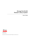
2. On the Instrument Setup page, mark the checkbox(es) that corresponds to the instrument(s)
installed on your PC, as shown in Fig. 1. To see more information on each instrument family,
click on the family name and read the corresponding Item Description on the right side of
the dialog.
If you already have ORTEC CONNECTIONS-32 MCBs attached to your PC, they will be
included on the Local Instrument List at the bottom of the dialog, along with any new
instruments. Existing (previously configured before this upgrade) instruments do not have to
be powered on during this part of the installation procedure.
NOTE You can enable other device drivers later, as described in Section 2.2.
3. If you want other computers in a network to be able to use your MCBs, leave the Allow
other computers to use this computer’s instruments marked so the MCB Server program
will be installed. Most users will leave this box marked for maximum flexibility.
NOTE If your PC uses Windows XP and you wish to use or share ORTEC MCBs across a
network, be sure to read Section 2.1.
4. Click on Done.
5. At the end of the wizard, restart the PC. Upon restart, remove the ScintiVision CD from the
drive.
5
ScintiVision®-32 v2 (A35-B32)
Fig. 1. Choose the Interface for Your Instruments.
6. After all processing for new plug-and-play devices has finished, you will be ready to
configure the MCBs in your system. Connect and power on all local and network ORTEC
instruments that you wish to use, as well as their associated PCs. Otherwise, the software will
not detect them during installation. Any instruments not detected can be configured at a later
time.
7. If any of the components on the network is a DSPEC® Plus, ORSIM II or III, MatchMaker,
DSPEC®, 92X-II, 919E, 920E, 921E, Ethernet-connected OCTÊTE, or other module that
uses an Ethernet connection, the network default protocol must be set to the IPX/SPX
Compatible Transport with NetBIOS selection on all PCs that use CONNECTIONS
hardware. For instructions on making this the default, see the network protocol setup
discussion in the MCB Properties Manual.
8. To start the MCB Configuration program on your PC, go to the Windows Start menu and
click on ScintiVision 32, and MCB Configuration. The MCB Configuration program will
locate all of the (powered-on) ORTEC MCBs attached to the local PC and to (powered-on)
network PCs, display the list of instruments found, allow you to enter customized instrument
numbers and descriptions, and optionally write this configuration to those other network
6
2. INSTALLING SCINTIVISION-32
PCs, as described in detail in the software installation chapter of the MCB Properties
Manual. If this is the first time you have installed ORTEC software on your system, be sure
to refer to the MCB Properties Manual for information on initial system configuration and
customization.
ScintiVision-32 is now ready to use, and its MCB pick list can be tailored to a specific list of
instruments (see Section 5.7.5).
2.1. If You Have Windows XP Service Pack 2 and Wish to Share
Your Local ORTEC MCBs Across a Network
NOTE If you do not have instruments connected directly to your PC or do not wish to share
your instruments, this section does not apply to you.
If you have installed Windows XP Service Pack 2 and have fully enabled the Windows Firewall,
as recommended by Microsoft, the default firewall settings will prevent other computers from
accessing the CONNECTIONS-32 MCBs connected directly to your PC. To share your locally
connected ORTEC instruments across a network, you must enable File and Printer Sharing on
the Windows Firewall Exceptions list. To do this:
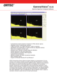
1. From the Windows Control Panel,
access the Windows Firewall entry.
Depending on the appearance of your
Control Panel, there are two ways to
do this. Either open the Windows
Firewall item (if displayed); or open
the Network Connections item then
choose Change Windows Firewall
Settings, as illustrated in Fig. 2. This
will open the Windows Firewall dialog.
Fig. 2. Change the Firewall Settings.
2. Go to the Exceptions tab, then click to mark the File and Printer Sharing checkbox (Fig. 3).
NOTE This affects only the ability of other users on your network to access your MCBs.
You are not required to turn on File and Printer Sharing in order to access
networked MCBs (as long as those PCs are configured to grant remote access).
3. To learn more about exceptions to the Windows Firewall, click on the What are the risks of
allowing exceptions link at the bottom of the dialog.
4. Click on OK to close the dialog. No restart is required.
7
ScintiVision®-32 v2 (A35-B32)
Fig. 3. Turn on File and Printer Sharing.
2.2. Enabling Additional ORTEC Device Drivers
You can enable other device drivers later with the Windows Add/Remove Programs utility on
the Control Panel. Select Connections 32 from the program list, choose Add/Remove, then
elect to Modify the software setup. This will reopen the Instrument Setup dialog so you can
mark or unmark the driver checkboxes as needed, close the dialog, restart the PC when
instructed, then re-run the MCB Configuration program as described in Step 8 on page 6.
8
3. GETTING STARTED TUTORIAL
3.1. Introduction
This chapter provides a series of straightforward examples to help you become familiar with
ScintiVision’s basic operations and move on quickly to full use. We will cover the following
functions:
!
!
!
!
!
!
!
Recalling a spectrum file from disk
Performing a simple analysis of the spectrum
Loading a nuclide library
Using the library editor
Energy calibration
Efficiency calibration
Getting a Detector ready for data acquisition
To display help for any of the dialogs, put the mouse pointer on the item and click the right
mouse button to display the
button. Now click the left mouse button to display the
help message. After reading the help message, click the left mouse button to close the message
box.
To make the discussion easier and more realistic, the sample files supplied on the ScintiVision
CD-ROM will be used in the following examples. Use Windows Explorer to verify that the
following files have been copied to your working directory, c:\User, during installation:
SVDEMO1.SPC
SVDEMO2.SPC
SVDEMO.ENT
SVDEMO.EFT
SVDEMO.LIB
Before we actually begin, here is a short note on the Detector and buffer concept used in
ScintiVision.
A spectrum can exist in three places in ScintiVision:
! In an MCB (which we call a Detector)
! In computer memory (a buffer)
! In a file on disk
The Detector is where the data are gathered from the HPGe detector. Data can be displayed and
manipulated directly in the Detector memory or a buffer. They can be copied from the Detector
to either the buffer or disk. Actions on the data in the buffer or spectrum file windows have no
effect on data acquisition taking place in a Detector — ScintiVision maintains separate
calibrations and viewing settings for each Detector, buffer, and spectrum file window.
9
ScintiVision®-32 v2 (A35-B32)
3.2. Starting ScintiVision
To start ScintiVision, go
to the Windows start menu
and click on ScintiVision 32,
ScintiVision (see Fig. 4).
ScintiVision will check for
Detectors, then display an
opening screen similar to
Fig. 5.
Fig. 4. Starting ScintiVision.
For illustrative purposes, this figure does not show an open spectrum window. However,
ScintiVision will attempt to open the last Detector displayed in the previous work session. If it
cannot find that Detector, no windows will open in the spectrum area.
Fig. 5. The ScintiVision Opening Screen.
10
3. GETTING STARTED TUTORIAL
3.2.1. Recalling a Spectrum
Open SVDEMO1.SPC as follows: On the
Menu Bar, click on File, then click on
Recall. This will open a dialog showing
the list of spectrum files in the current
directory,2 as shown in Fig. 6. From the list
of files, double-click on SVDEMO1.SPC, or
click once on the file name then click on
OK. SVDEMO1.SPC will be displayed in a
window as shown in Fig. 7. The Status
Sidebar on the right of the screen will now
show details about this spectrum. When a
second spectrum is recalled, it will be
displayed in a second window, and so on.
Fig. 6. Recalling a Spectrum File.
The sidebar will show details for the
spectrum in the active window (click on a
portion of an inactive window to activate it).
Note the vertical marker line, which you can move by clicking the left mouse button on a
different part of the spectrum. The Marker Information Line at the bottom of the display reflects
the channel contents at the marker’s location. You can tell that this spectrum is already
calibrated because the information about the marker reads in units of energy, keV. (An
uncalibrated spectrum would instead display the word uncal.)
2
If the spectrum files listed on page 11 are not present, the working directory is probably not set to C:\User. Click
on the Look in droplist and select C:\User as your working directory.
11
ScintiVision®-32 v2 (A35-B32)
Fig. 7. Calibrated Spectrum Recalled from Disk File.
3.2.2. The Simplest Way To Do An Analysis
Select a portion of the SVDEMO1.SPC spectrum for analysis by positioning the mouse on or near
the 1332-keV peak in the Full Spectrum View (Fig. 8), which will be located near the upper left
edge of the window, and clicking the left mouse button. This will move the marker to the mouse
pointer. The Expanded Spectrum View will now show this part of the spectrum.
Now zoom in on this part of the
spectrum by going to the Toolbar and
clicking on the Zoom In button ( )
five or six times. As you click, note that
the Full Spectrum View will show the
portion of the spectrum that you are
Fig. 8. Full Spectrum View.
zooming, and the Expanded Spectrum
View will display this part of the
spectrum (see Fig. 7). If the 1332-keV
region is not on the screen, click on the peaks in the right side of the Full Spectrum View to
reposition the zoomed region.
12
3. GETTING STARTED TUTORIAL
Once you have zoomed in on the 1332-keV peak, go to the
Menu Bar and click on Analyze, then Interactive in viewed
area... (see Fig. 9). ScintiVision will automatically analyze the
selected region and display the results. The Analysis Sidebar
will open (it is shown superimposed on the Status Sidebar in
Fig. 10). The peak fit(s) will be shown graphically, and the
numerical results will be displayed in an Analysis Results
Table window, as shown in Fig. 10.
That’s all it takes to do an analysis!
Fig. 9. Analyze/Interactive in
Viewed Area.
There are several functions you can access at this point, but
first we will load a working nuclide library and check some
parameters. Exit this analysis session by clicking on the Analysis Sidebar’s Close button (
This will close the Analysis Sidebar and the Analysis Results Table.
).
Fig. 10. Completed Analysis, Showing Results Table and Analysis Sidebar.
13
ScintiVision®-32 v2 (A35-B32)
3.2.3. Loading a Library
From the Menu Bar, select Library, then Select File... as shown in
Fig. 11. This will open a list of nuclide libraries in the current directory.
Select the library file SVDEMO.LIB and click on OK to load it. The
following message will appear on the Supplemental Information Line at
the bottom of the ScintiVision window:
SVdemo.lib: 3 Nuclides (13 alloc.); 5 Peaks (20 alloc.)
Fig. 11. Load a
Library from
Menu.
This message describes the library just loaded. SVDEMO.LIB contains 3 nuclides with space for
13, and has 5 peaks with space for 20.
This library, SVDEMO.LIB, is now loaded into the computer memory, and ScintiVision will use it
for all analyses until you choose another library. Until you choose another, SVDEMO.LIB will
automatically be reloaded each time ScintiVision is started.
3.2.4. Setting the Analysis Parameters
Click on Analyze, then Settings. From
the submenu that opens (Fig. 12), select
Sample Type.... This will open the
Analysis Options dialog shown in
Fig. 13. These sample type settings
allow you to specify the various analysis
parameters for analysis of the currently
displayed spectrum. In routine use, these
would not be changed, except for the
Fig. 12. Selecting the Sample Type... Command.
Sample Description. The entry of
Sample Weight and Sample Description
can be automated using the Acquisition Settings... command under the Acquire menu.
The Nuclide Library is the one just loaded in computer memory. The Calibration is the
calibration in computer memory, in this case, the calibration that was stored in SvDemo1.Spc
and recalled along with the spectrum.
Select the Report tab to view the output options (Fig. 14).
To send the output to a printer (as well as a file), go to the Output section of the screen and
click on the Printer radio button to mark it with a dot.
14
3. GETTING STARTED TUTORIAL
To send the output to a file only, click on the File radio button, and leave the asterisk ( * ) as the
filename.
To send the output to a text processing program, such as Windows Notepad (which is the
default), click on the Program radio button.
Click on all four checkboxes in the Reporting Options section of the screen, then click on OK.
Select Analyze and Entire spectrum in memory... to start the analysis. Once the “hourglass”
has disappeared from the screen, you can continue with other system operations while the
analysis runs to completion. The computer will beep when the analysis is complete. Spectra can
be analyzed in a buffer (as we have done here), directly from disk, or in the Detector memory
(when the Detector is not counting). If more than one window is open at one time, the spectrum
in the active window will be the one analyzed.
Fig. 13. Analysis Options Dialog, Sample Tab.
15
ScintiVision®-32 v2 (A35-B32)
Fig. 14. Analysis Options Dialog, Report Tab.
While the analysis is taking place, put the marker on the peak at 136 keV and expand the display
horizontally with Zoom In.
After the analysis is complete, the results will be printed or saved to disk (according to your
selection on the Report tab on the Analysis Options dialog). They can also be graphically
displayed by selecting Analyze and Display Analysis Results..., then clicking on Open to load
the analysis results file, SVDEMO.UFO. This will overlay the peak shapes on the spectrum data,
open the Analysis Results Table for the spectrum, and display the Analysis Sidebar
superimposed over the Status Sidebar, as shown in Fig. 15. Zoom in to see more details.
Put the mouse on the 137Cs (661.6 keV) entry in the peak list table and click. The marker will
move to that peak in the display. You can use the scroll bars on the peak list window to show
other energies, and then when you click on the energy, the display will show that peak.
In this mode, you can also use the buttons on the Analysis Sidebar to move the marker in the
spectrum. For example, click on 137Cs in the peak table, then click on
(the right-hand
Energy button in the Library Peak section of the Analysis Sidebar) to put the marker on the
next-highest-energy library peak, which is the 1173.2-keV line of 60Co. Note that this peak is
now highlighted in the Analysis Results Table.
16
3. GETTING STARTED TUTORIAL
Fig. 15. Display Analysis Results.
Now click on
to go to the next-highest-energy peak in the library for 60Co. The within
Nuclide buttons are useful for checking if other peaks for the nuclide exist so that you can
confirm their identity. The
button moves the marker in reverse order through the peaks
for the selected nuclide.
The
buttons are used to select the spectrum peaks that are not associated with a
library energy. This is useful to see if there are any unidentified spectrum peaks that should be
considered in the complete analysis.
The
buttons are used to select the regions with overlapping peaks. With these, you
can easily check how the analysis of complicated regions was handled.
Now, select Library and Select Peak... to show a list of the peaks in the current library.3 You
can use this list of peaks to move around in the spectrum. Click on the Library List window’s
3
This may be a different library than the one used in the analysis of the spectrum.
17
ScintiVision®-32 v2 (A35-B32)
down arrow to scroll down to 122-keV 57Co. Now click on this entry and the display will update
to this peak.
Exit this analysis session by clicking on the Analysis Sidebar’s Close button ( ). This will
close the Analysis Sidebar and the Analysis Results List window. Leave the Library List
window open.
3.2.5. Energy Calibration
For this example, we will use the spectrum files supplied with
ScintiVision to recalibrate the buffer. The same procedure is
used to calibrate the Detector spectrum.
The display should be showing the SVDEMO1.SPC spectrum
window and Library List window. If the complete library peak
list is not visible, you can click and drag the window edges to
resize it.
From the Calibrate menu (Fig. 16), select Energy.... The
Energy Calibration Sidebar (Fig. 17), will open superimposed
on the Status Sidebar. Note that you can move this sidebar by
clicking and dragging the”Calibr...” title bar. (You can also
move the other windows the same way.)
Fig. 16. Start Energy
Calibration from Menu.
This time, so that we’re starting from the very beginning, we will destroy
the current energy calibration by clicking on the icon to the left of the title
“Calib...”. This will open the control menu shown in Fig. 18. Click on
Destroy. The Marker Information Line now shows the legend uncal.
Move the cursor to channel 401, the location of the upper 60Co peak, at
1332.5 keV. Do this directly in the Full Spectrum View or by using the
buttons until you get there. Click once in the E= field at the
top of the Calibration Sidebar, enter the correct energy for this peak
(1332.5 keV), mark an ROI, and click on Enter. The system will
automatically perform a simple calibration based on this peak and the
assumption that channel zero is energy zero. The graphs of the calibration
and the table of values will be displayed, as shown in Fig. 19.
If the screen becomes too visually crowded, you can move one or more
windows until they are nearly “stacked” atop each other (leave at least an
edge or corner of each window showing); or close one or more windows by
clicking on their Close box ( ). However, do not close the Calibration
18
Fig. 17. Energy
Calibration
Sidebar.
3. GETTING STARTED TUTORIAL
Sidebar or you’ll end the calibration session. Remember, you can bring a window to the front by
clicking on any part of it (if it’s not visible, move one or more of the others until you can see it).
Now we can use the library. Double-click on the 661.62-keV peak of 137Cs
in the library list. The marker will move close to, but not precisely on, that
peak in the spectrum, based on our current “one-point calibration.” Use the
buttons to put the cursor on the peak, then click once on the
661.62-keV entry in the library list. Note that the E= 661.62 keV in the
Calibration Sidebar already has the appropriate energy from the library, and
you need only accept it by marking an ROI and clicking on Enter. The refitted calibration curve is automatically displayed.
Fig. 18. Energy
Calibration Sidebar
Control Menu.
Fig. 19. Energy Calibration Display.
19
ScintiVision®-32 v2 (A35-B32)
Proceed through the library list (see Table 1), adding the following
peaks (in any order) into the calibration. To do this, double-click on
the peak energy in the library list, look at the display to see that the
cursor is on the peak, then click on Enter.
If you decide that you don’t want one of the peaks, just delete it by
clicking on the Delete Energy button on the Calibration Sidebar.
Now bring the Energy Table window to the front, and note that the
Deltas (the differences between data points and the fit to the data
points) are small. Next, bring the Energy plot window to the front
and examine the calibration curve visually. You can, of course,
increase the size of these windows to allow a closer examination of
the graphical fit.
Table 1. Source Energies.
Nuclide
88
Energy (keV)
Y
1836.01
57
Co
122.07
60
Co
1173.2
60
Co
1332.51
88
Y
898.02
137
Cs
661.66
113
Sn
391.69
203
Hg
279.17
109
Cd
88.03
241
Am
59.54
Click on the FWHM (full width at half maximum) radio
button on the lower section of the Calibration Sidebar.
This will change the table and calibration windows so
they now display the table of FWHM results and the
FWHM graph, as in Fig. 20. The FWHM fit uses the
peaks specified in the energy fit. If FWHM of any peak
has a deviation of more than 25% between the actual
and fitted values, a warning message is displayed.
Fig. 20. FWHM Fit Selection.
Save the energy table for later use: click on the Calibration
Sidebar’s Save button, enter a name such as SVDEMO for
the table filename, and click on Save. ScintiVision will append the correct extension, .ENT, to
the filename. To examine the Energy Table, open the Calibration Sidebar’s control menu and
select Edit File. This table is simply a list of the energies of the peaks used for the calibration.
The energy calibration is complete; we shall consider this to be a “good” energy calibration for
the purposes of this demonstration. Close the calibration session by opening the control menu in
the calibration window and selecting Close.
This new energy calibration is now held in memory but is not yet stored on disk.
20
3. GETTING STARTED TUTORIAL
3.2.6. Efficiency Calibration
Select Calibrate from the Menu Bar, then Efficiency. This opens the
Efficiency Calibration Sidebar, shown in Fig. 21 (note its similarity to the
Energy Calibration Sidebar).
We want to start from the beginning of the process, so open the sidebar’s
control menu and click on Destroy.
The Library List window should be visible, but if not, click on Library/
Select Peak... to reopen it.
From the library, double-click on the 1332.5-keV peak of 60Co. When you
double-click, the marker will move to the corresponding peak and
ScintiVision will enter the energy in the top section of the Calibration
Sidebar.
In the upper section of the sidebar, click on the Calc... button to open the
Efficiency Calculation Worksheet (Fig. 22).
Fig. 21.
Efficiency
Calibration
Sidebar.
Fig. 22. Efficiency Worksheet.
21
ScintiVision®-32 v2 (A35-B32)
Enter the date and the time from the calibration
certificate (see Table 2), as 30-Oct-92 and
12:00:00. Enter the gammas per second (19671)
from the calibration certificate for 60Co at
1332.5 keV. Select GPS from the units drop-list.
Note that the from Library box is checked; this
shows that the half-life came from the library.
Table 2. List of Peak Energies.
Reference time 12:00 GMT 30 Oct 1992
Nuclide
57
Co
Cs
60
Co
60
Co
137
Energy (keV)
Gammas/sec
122.1
661.63
1173.2
1332.5
15920
15598
19640
19671
At this point, the Calculate Efficiency= button
at the top of the worksheet should be active
(black rather than gray). If it is gray, one or more of the data inputs is either incorrect or has not
been entered. When you have completed all fields and Calculate Efficiency= is activated, click
on it to obtain the efficiency value at this energy. Click on OK to insert the value in the
efficiency table. You will see that the value appears in the Efficiency Table window.
You could repeat this process for all other peaks in the calibration certificate data, but there is an
easier way. All of the information from the calibration certificate can be stored in an efficiency
calibration (.EFT) file (see “Editing the Efficiency Calibration Table” on page 104 for
instructions on creating and editing this file). Using this file to direct the calibration is easy. On
the Efficiency Calibration Sidebar, just click on the Recall... button, then select the file
SVDEMO.EFT. ScintiVision will use the data in the table to calculate the efficiency at each energy
from the spectrum and fill in the efficiency table. You can see the marker jump from peak to
peak in the spectrum as the peak areas are calculated.
When the data points are all calculated, the fit Mode stored in the file is used to make the fit.
You can select another fit Mode from the Calibration Sidebar. In the list, choose the Polynomial
option. This will automatically produce a quadratic fit of the entire energy range, as shown in
Fig. 23.
The fit will take place automatically. You can then view it by bringing the Efficiency calibration
fit window forward. Click on the window’s control menu to choose scaling and grid display
options (see Fig. 24). The marker line in the efficiency graph window will be at the energy of the
peak selected in the Library List or the Efficiency Table window.
22
3. GETTING STARTED TUTORIAL
Fig. 23. Polynomial Efficiency Fit.
We will accept this calibration and close the calibration session by clicking
on the Calibration Sidebar’s Close button. Now save this calibration to disk
by selecting Calibrate and Save Calibration.... Give the calibration file
the name SVDEMO. ScintiVision will attach the default .CLS extension to
the filename.
3.2.7. Changing a Library
Select Library/Edit/ScintiVision Editor... from the Menu Bar. This will
open the Editing dialog (Fig. 25), which allows you to change, add, or delete
nuclide and gamma-ray values in the currently loaded nuclide library file.
Fig. 24. Efficiency
Fit Window
Control Menu.
Select the nuclide 60Co from the left-hand section of the dialog. All the
gamma-ray energies or peaks for this nuclide will then appear in the Peaks section; select the
23
ScintiVision®-32 v2 (A35-B32)
1332.5-keV peak. Click on Edit... in the Peaks section. This will open the Edit Library Peak
dialog (Fig. 26), which will show the current values and allow you to change the energy and
gammas-per-disintegration of the 1332.5-keV line.
Fig. 25. Edit Nuclide Library with ScintiVision Editor.
Click on the Gammas per 100 disintegrations field
and change the value, then click on OK. You will see
that the Gammas per 100 Disintegrations value for
this peak has been changed to the number you just
entered.
Now click on the Editing dialog’s Close button to
leave the library editor. When asked if you want to
save the modified library, click on No to ignore the
change you just made in the Gammas per 100
Disintegrations field.
The ScintiVision library editor is explained in detail
in Section 5.6. Note that ScintiVision can also use
NuclideNavigator III libraries as master libraries
24
Fig. 26. Edit Nuclide Peak.
3. GETTING STARTED TUTORIAL
(not analysis libraries), and that you can access NuclideNavigator III directly from the
ScintiVision Library/Edit submenu if the NuclideNavigator package is installed on your PC.
3.2.8. Detector Setup
Before starting data collection, make sure the detector, analog electronics (in older systems), and
MCB are connected and powered on according to their respective hardware manuals.
The ScintiVision installation program will have already located the Detectors available to this
PC. Click on the Detector pick list on the right of the Toolbar and select a Detector. The
spectrum displays will update to show the data in this Detector.
In the simplest mode of operation, data acquisition is
started from the Toolbar; simply click on the Start button.
You can use the Acquire menu (Fig. 27) to check the
analysis settings while data is being gathered. After
acquisition stops, the analysis can proceed.
All of ScintiVision’s hardware setup controls are now
in one, MCB-specific dialog. Depending on your Detector,
this might include controls for conversion gain, amplifier,
high voltage, shaping, data acquisition presets, and more.
To access this dialog, click on Acquire/MCB Properties...,
or right-click the mouse to open its menu and select MCB
Properties.
Fig. 27. Acquire Menu.
Some of the Detector’s internal parameters can only be
changed when the Detector is not acquiring data. To see if the Detector is in acquisition mode,
open the Acquire menu look at the menu items. If Stop is black and Start is gray (note that
Fig. 27 shows the opposite case), the Detector is in acquisition mode.4 If this is the case, select
Stop from the menu or Toolbar.
4
We say “acquiring data” when the MCB is in acquisition mode, even if there are no counts accumulating in the
MCB.
25
ScintiVision®-32 v2 (A35-B32)
3.2.8.1. Conversion Gain
If you wish to change the conversion gain, click on Acquire/MCB
Properties..., select the ADC tab
(Fig. 28), then change the Conversion
Gain field. The ADC gain is stored in
the MCB and automatically recalled
from the MCB the next time you
restart ScintiVision. Note that in
this example, we are using a 92X-II,
and that the Properties dialog
automatically displays only data fields
that are applicable to this MCB.
Fig. 28. Setting the 92X-II Conversion Gain.
If you have computer-controlled
hardware, skip to Section 3.2.8.3.
3.2.8.2. Detectors Set Up Manually
Manually adjust the spectroscopy amplifier gain, shaping time, and pole zero according to the
instructions in the amplifier manual. Most commonly, a range of 0!3 MeV is used. If you have a
60
Co source, the 1332-keV peak should be set at approximately channel 1816 for conversion
gain of 4096 and channel 3632 for 8192. A source with only one or two lines (e.g., 137Cs or 60Co)
should be used for the initial test spectrum so you’ll be able to easily see the correct pattern of
the peaks.
3.2.8.3. Computer-Controlled Hardware Setup
In this section, we will use
ScintiVision to enable the 92X-II’s
high voltage and adjust the
spectroscopy amplifier gain,
shaping time, and pole zero.
Select Acquire/MCB Properties...
to open the Properties dialog for this
MCB, and click on the High Voltage
tab (see Fig. 29).
Adjust the bias setting to the correct
voltage on the rear panel of the 92X-II.
Notice, as you adjust the voltage, that
26
Fig. 29. Monitoring the 92X-II Bias Setting on the High
Voltage Tab.
3. GETTING STARTED TUTORIAL
the value showing in the Target field on the High Voltage tab changes. The display setting is
accurate to ±100 V.
When the value of the detector bias matches that shown on the detector’s Quality Assurance data
sheet (also given on the endcap label), click the On button to enable the bias. The HV On light
on the 92X-II will illuminate. If it does not, either the HV shutdown is not connected or the
detector is warm. (The detector might require 3–6 hours after filling before it is cold enough to
take bias.)
3.2.8.4. Amplifier Settings
Click on the Amplifier tab (Fig. 30).
The amplifier shaping time can be set
to either Long or Short. The Long
shaping time is the recommended
choice for low to moderate count rates.
The value of the shaping time (in µs)
is given in the hardware manual.
If you have a transistor-reset preamplifier (Plus Series), select it from
the Preamplifier Type droplist. Skip
the following subsection on polezeroing and go to the discussion on
adjusting amplifier gain.
Fig. 30. The 92X-II Amplifier Tab.
Click on Close to apply the new MCB hardware settings.
Automatic Pole Zero5
Select Acquire, then Start, to start the Detector counting. Next, place a
source such as 60Co, of sufficient strength to produce a few percent dead
time, in the Detector. During data collection, the dead time is shown on the
center right of the display, as in Fig. 31.
Next, return to Acquire/MCB Properties... and click on the Amplifier tab.
Fig. 31.
Go to the Pole Zero section of the dialog and click on Start Auto. This will
Dead Time.
tell the Detector to automatically adjust the pole zero of the amplifier. While
the pole-zero adjustment is in progress, you will hear a periodic beep and see
the message “Auto PZ in progress....” The time needed for the pole zero depends on the activity
5
U.S. Patents 4,866,400 and 5,872,363.
27
ScintiVision®-32 v2 (A35-B32)
of the source and how far the pole zero is out of adjustment. No more than a minute or two
should be required. Remember that if you change the shaping time, you must pole zero the
Detector again.
Click on Close to apply the new MCB hardware settings.
Adjusting Amplifier Gain
Now adjust the amplifier gain to achieve the desired energy range across the Detector display.
Most commonly, a range of 0–3 MeV is used. If you have a 60Co source, the 1332-keV peak
should be set at approximately channel 1816 for conversion gain of 4096, and channel 3632 ofor
8192 (see Fig. 32). A source with only one or two lines (e.g., 137Cs or 60Co) should be used for
the initial test spectrum so you’ll be able to easily see the correct pattern of the peaks. To set the
gain for the 92X-II (as well as the DSPEC Plus, DSPEC, 92X, DART, and NOMAD Plus):
Fig. 32. Spectrum with 60Co.
1. Start data collection by clicking on the Start Toolbar button or by selecting Acquire/Start
from the Menu Bar.
2. Select Acquire/MCB Properties... and click on the Amplifier tab (Fig. 30).
28
3. GETTING STARTED TUTORIAL
3. Select the Coarse Gain setting from the droplist, then move the slider to the fine gain
desired. The spectrum display is not continuously updated while the Properties dialog is
open, but you can force an immediate spectrum update by moving the control dialog over the
spectrum window, releasing it, then moving it away so the spectrum will redraw.
4. Once the gain is approximately correct, click on Close to close the control dialog, then use
<Alt + +> and <Alt + !> to make fine gain adjustments until the peak is in the desired
channel. To make coarser gain adjustments, use <Alt + Shift + +> and <Alt + Shift + !>.
(These keyboard commands are discussed in Chapter 9.)
ScintiVision will retain all of these settings and adjustments on exit, and will reload them from
the MCB on restart. You are now ready to acquire spectral data, calibrate, and analyze your own
sample data.
29
ScintiVision®-32 v2 (A35-B32)
30
4. DISPLAY FEATURES
This chapter addresses ScintiVision’s display features, discusses the role of the mouse and
keyboard, covers the use of the Toolbar and sidebars, and shows how to change to different disk
drives and folders.
Figure 33 shows ScintiVision’s principal screen features.
Fig. 33. Main ScintiVision Screen Features.
1. Title bar, showing the source of the currently displayed spectrum. This is either the Detector
description; the word “Buffer” if the buffer is selected; or a file name, if a file has been
saved or recalled and not yet modified (if a sample description has been entered for the file,
it will accompany the file name). On the far right are the Minimize, Maximize, and Close
buttons.
2. Menu Bar, showing the available menu commands (which can be selected with either the
mouse or keyboard); these functions are discussed in detail in Chapter 5.
31
ScintiVision®-32 v2 (A35-B32)
3. Toolbar, beneath the Menu Bar, contains icons for recalling spectra, saving them to disk,
starting and stopping data acquisition, changing the point/fill characteristics of a spectrum,
and adjusting the spectrum’s vertical and horizontal scale. The name of the last Detector
selected is shown.
4. Drop-down Detector List, on the Toolbar, displaying the currently selected Detector (or the
buffer). Clicking on this field opens a list of all Detectors currently on the PC’s ScintiVision
Detector pick list, from which you can select a Detector or the buffer.
5. Spectrum Area, which can display one or more windows of data from Detectors, buffers, or
spectrum files. These windows can be moved, sized, minimized, maximized, and closed with
the mouse, as well as tiled horizontally or vertically from the Window menu. When more
than one window is open, only one is active — available for data manipulation and analysis
— at a time. The Title Bar on inactive windows will be gray (unless you have changed the
color scheme in Windows Control Panel) while the active window’s title bar will be a
brighter color. To switch windows, click on the window you wish to view, or cycle between
windows by pressing <Ctrl + Tab>.
Each spectrum window contains a Full Spectrum View and an Expanded Spectrum View (see
items 6 and 7 below).
6. The Full Spectrum View shows the full histogram from the file or the Detector memory.
The vertical scale is always logarithmic, and the window can be moved and sized (see
Section 4.3.4). The Full Spectrum View contains a rectangular window that marks the
portion of spectrum now displayed in the Expanded Spectrum View. To quickly move to
different part of the spectrum, just click on that area in the Full Spectrum View and the
expanded display updates immediately at the new position.
7. The Expanded Spectrum View shows all or part of the full histogram; this allows you to
zoom in on a particular part of the spectrum and see it in more detail. You can change the
expanded view’s vertical and horizontal scaling, and perform a number of analytical
operations such as peak information, marking ROIs, or calibrating the spectrum. This
window contains a vertical line called a marker that highlights a particular position in the
spectrum. Information about that position is displayed on the Marker Information Line (see
item 10 below).
8. ROI Status Area, on the right side of the menu bar, indicates whether the ROI marking
mode is currently Mark, UnMark, or Off. This operates in conjunction with the ROI menu
commands and arrow keys (see Section 5.8).
32
4. DISPLAY FEATURES
9. Status Sidebar, on the right side of the screen, providing information on the current
Detector presets and counting times, the time and date, and a set of buttons that allow you to
move easily between peaks, ROIs, and library entries (see Section 4.4).
10. Marker Information Line, beneath the spectrum, showing the marker channel, calibration,
and contents.
11. Supplementary Information Line, below the Marker Information Line, used to show
library contents, the results of certain calculations, warning messages, or instructions.
4.1. Spectrum Displays
The Full and Expanded Spectrum Views show, respectively, a complete histogram of the current
spectrum (whether from a Detector or buffer) and an expanded view of all or part of the
spectrum. These two windows are the central features of the ScintiVision-32 screen. All other
windows and most functions relate to the spectrum windows. The Full Spectrum View shows the
entire data memory of the Detector as defined in the configuration. In addition, it has a marker
box showing which portion of the spectrum is displayed in the Expanded Spectrum View.
The Expanded Spectrum View contains a reverse-color marker line at the horizontal position of
the pixel representing the marker channel. This marker can be moved with the mouse pointer, as
described in Section 4.3.1, and with the <7>/<6> and <PgUp>/<PgDn> keys.
The spectrum display can be expanded to show more detail or contracted to show more data
using the Zoom In and Zoom Out features.6 Zooming in and out can be performed using the
Toolbar buttons, the Display menu commands, or the rubber rectangle (see Section 4.3.3). The
rubber rectangle allows the spectrum to be expanded to any horizontal or vertical scale. The
baseline or “zero level” at the bottom of the display can also be offset with this tool, allowing
the greatest possible flexibility in showing the spectrum in any detail.
The Toolbar and Display menu zoom commands offer a quick way to change the display. These
change both the horizontal and vertical scales at the same time. For Zoom In, the horizontal
width is reduced by about 6% of full width (ADC conversion gain) and the vertical scale is
halved. The Zoom In button and menu item zoom to a minimum horizontal scale of 6% of the
ADC conversion gain. For Zoom Out, the horizontal width is increased by about 6% of full
width (ADC conversion gain) and the vertical scale is doubled.
6
These replace the Narrower/Wider and Shorter/Taller commands in older versions of ScintiVision.
33
ScintiVision®-32 v2 (A35-B32)
The Keypad<+> and Keypad<!> accelerator keys duplicate the Zoom In and Zoom Out
Toolbar buttons and Display menu commands. The <F5>/<F6> and <9>/<8> keys change the
vertical scale by a factor of two without changing the horizontal scale. The <F7>/<F8> and
keyboard <!>/<+> keys change the horizontal scale by a factor of two without changing the
vertical scale.
Depending on the expansion or overall size of the spectrum, all or part of the selected spectrum
can be shown in the expanded view. Therefore, the number of channels could be larger than the
horizontal size of the window, as measured in pixels. In this case, where the number of channels
shown exceeds the window size, all of the channels cannot be represented by exactly one pixel
dot. Instead, the channels are grouped together, and the vertical displacement corresponding to
the maximum channel in each group is displayed. This maintains a meaningful representation of
the relative peak heights in the spectrum. For a more precise representation of the peak shapes
displaying all available data (i.e., where each pixel corresponds to exactly one channel), the
scale should be expanded until the number of channels is less than or equal to the size of the
window.
Note that the marker can be moved by no less than one pixel or one channel (whichever is
greater) at a time. In the scenario described above, where there are many more memory channels
being represented on the display than there are pixels horizontally in the window, the marker
will move by more than one memory channel at a time, even with the smallest possible change
as performed with the <6> and <7> keys. If true single-channel motions are required, the
display must be expanded as described above.
In addition to changing the scaling of the spectrum, the colors of the various spectrum features
(e.g., background, spectrum, ROIs) can be changed using the Display menu.
4.2. The Toolbar
The row of buttons below the Menu Bar provides convenient shortcuts to some of the most
common ScintiVision menu functions.
The Recall button retrieves an existing spectrum file. This is the equivalent of selecting
File/Recall from the menu.
Save copies the currently displayed spectrum to disk. It duplicates the menu functions
File/Save or File/Save As... (depending on whether the spectrum was recalled from disk,
and whether any changes have been made to the spectrum window since the last save).
34
4. DISPLAY FEATURES
Start Acquisition starts data collection in the current Detector. This duplicates
Acquire/Start and <Alt + 1>.
Stop Acquisition stops data collection. This duplicates Acquire/Stop and <Alt + 2>.
Clear Spectrum clears the detector or file spectrum from the window. This duplicates
Acquire/Clear and <Alt + 3>.
Mark ROI automatically marks an ROI in the spectrum at the marker position, according
to the criteria in Section 5.8.4. This duplicates ROI/Mark Peak and <Insert>.
Clear ROI removes the ROI mark from the channels of the peak currently selected with
the marker. This duplicates ROI/Clear and <Delete>.
The next section of the Toolbar (Fig. 34) contains the buttons that control
the spectrum’s vertical scale. These commands are also on the Display
menu. In addition, vertical scale can be adjusted by zooming in with the
mouse (see Fig. 40).
Fig. 34. Vertical
Scaling Section of
Toolbar.
Vertical Log/Lin Scale switches between logarithmic and linear
scaling. When switching from logarithmic to linear, it uses the previous linear scale
setting. Its keyboard duplicate is Keypad</>.
Vertical Auto Scale turns on the autoscale mode, a linear scale that automatically
adjusts until the largest peak shown is at its maximum height without overflowing the
display. Its keyboard duplicate is Keypad<*>.
The field to the left of these two buttons displays LOG if the scale is logarithmic, or indicates
the current vertical full-scale linear value.
The horizontal scaling section (Fig. 35) follows next. It includes
a field that shows the current window width in channels, and the
Fig. 35. Horizontal Scaling
Zoom In, Zoom Out, Center, and Baseline Zero buttons. These
Section of Toolbar.
commands are also on the Display menu. In addition, horizontal
scale can be adjusted by zooming in with the mouse (see Fig. 40).
Zoom In decreases the horizontal full scale of the Expanded Spectrum View according to
the discussion in Section 4.1, so the peaks appear “magnified.” This duplicates
Display/Zoom In and Keypad<+>.
35
ScintiVision®-32 v2 (A35-B32)
Zoom Out increases the horizontal full scale of the Expanded Spectrum View according
to the discussion in Section 4.1, so the peaks appear reduced in size. This duplicates
Display/Zoom Out and Keypad<!>.
Center moves the marker to the center of the screen by shifting the spectrum without
moving the marker from its current channel. This duplicates Display/Center and
Keypad<5>.
Baseline Zero switches to autoscale mode and sets the baseline of the Expanded
Spectrum View to zero. Autoscale is then switched off.
NOTE
In addition to the preceding commands, note the Full View command on the Display
menu (duplicated by <Alt+F7>). This function adjusts the horizontal and vertical
scaling to display the entire spectrum in the Expanded Spectrum View.
The right-most part of the Toolbar is a droplist of the available
Detectors (Fig. 36). To select a Detector or the buffer, click in the
field or on the down-arrow beside it to open the list, then click on
the desired entry. The sidebar will register your selection.
Finally, note that as you pause the mouse pointer over the center of a
Toolbar button, a pop-up tool tip box opens, describing the button’s
function (Fig. 37).
Fig. 36. Drop-Down
Detector List.
4.3. Using the Mouse
The mouse can be used to access the menus, Toolbar, and sidebars; adjust
spectrum scaling; mark and unmark peaks and ROIs; select Detectors; work
in the dialogs — every function in ScintiVision except text entry. For most
people, this might be more efficient than using the keyboard. The following
sections describe specialized mouse functions.
Fig. 37. Tool Tip.
4.3.1. Moving the Marker with the Mouse
To position the marker with the mouse, move the pointer to the desired channel in the Expanded
Spectrum View and click the left mouse button once. This will move the marker to the mouse
position. Click in the Full Spectrum View to move the expanded view to that place. This is
generally a much easier way to move the marker around in the spectrum than using the arrow
keys and accelerators, although you might prefer to mix mouse and keyboard commands.
36
4. DISPLAY FEATURES
4.3.2. The Right-Mouse-Button Menu
Figure 38 shows the right-mouse-button menu. To open it, position the
mouse pointer in the spectrum display, click the right mouse button, then
use the left mouse button to select from its list of commands. Not all of the
commands are available at all times, depending on the spectrum displayed
and whether the rubber rectangle is active. Except for Undo Zoom In, all
of these functions are on the Toolbar and/or the Menu Bar (Peak Info,
Input Count Rate, and Sum are only on the Menu Bar, under Calculate).
See Section 5.10 for more information on the commands.
4.3.3. Using the “Rubber Rectangle”
The rubber rectangle is used for selecting a particular area of interest
within a spectrum. It can be used in conjunction with the right-mousebutton menu in Fig. 38 for many functions. To draw a rubber
rectangle:
Fig. 38. RightMouse-Button
Menu for Spectra.
1. Click and hold the left mouse button; this anchors the starting
corner of the rectangle.
2. Drag the mouse diagonally across the area of interest. As you
do this, the mouse will be drawing a reverse-color rectangle
bisected by the marker line. Note that when drawing a rubber
rectangle, the marker line combines with a horizontal line inside
the rectangle to form crosshairs (Fig. 39). They make it easy to
select the center channel in the area of interest — this might be
the center of an ROI that you wish to mark or unmark, a portion
of the spectrum to be summed, or a peak for which you
want detailed information.
3. Release the mouse button; this anchors the ending corner of the
rectangle.
Fig. 39. The Rubber
Rectangle’s Crosshairs.
4. Click the right mouse button to open its menu, and select one of
the available commands. Once an area is selected, the commands
can also be issued from the Toolbar, Menu Bar, Status Sidebar, or keyboard.
As an example, Fig. 40 illustrates the process of marking a region with a rubber rectangle and
zooming in using the right-mouse-button menu.
37
ScintiVision®-32 v2 (A35-B32)
Fig. 40. Zooming In Using the Rubber Rectangle and
Right-Mouse-Button Menu.
You can move the rectangle using the arrow keys. The
<Shift + 7> and <Shift + 6> keys move the box left
and right, while <Shift + 8> and <Shift + 9> move
the box up and down. This enables you to position the
box more precisely.
4.3.4. Sizing and Moving the Full Spectrum
View
To change the horizontal and vertical size of the Full
Spectrum View, move the mouse pointer onto the side
edge, bottom edge, or corner of the window until the
pointer changes to a double-sided arrow (see Fig. 41).
Click and hold the left mouse button, drag the edge of
the window until it is the size you want, then release
the mouse button.
38
Fig. 41. Two-Sided Pointer for Sizing Full
Spectrum View, and Four-Sided Pointer for
Moving Window.
4. DISPLAY FEATURES
To move the Full Spectrum View to a different part of the screen, move the mouse pointer onto
the top edge of the window until the pointer changes to a four-sided arrow (see Fig. 41). Click
and hold the left mouse button, drag the window to its new location, and release the mouse
button.
4.4. Buttons and Boxes
This section describes ScintiVision’s radio buttons, indexing buttons, and checkboxes. To
activate a button or box, just click on it.
Radio buttons (Fig. 42) appear on many ScintiVision dialogs,
and allow you to select of only one of the choices.
Checkboxes (Fig. 43) are another common feature, allowing
you to select one or more of the options at the same time.
Fig. 42. Radio Buttons.
The ROI, Peak, and Library indexing buttons on the Status
Sidebar are useful for rapidly locating ROIs or peaks, and for
advancing between entries in the library. When the last item in
either direction is reached, the computer beeps and ScintiVision
posts a “no more” message on the Supplementary Information
Line. If a library file has not been loaded or the Detector is not
calibrated, the Library buttons are disabled and shown in gray.
Fig. 43. Checkboxes.
The indexing buttons are displayed in two different ways, depending
on whether ScintiVision is in Detector or buffer mode. This is shown in Fig. 44.
In Detector mode, the buttons appear at the bottom of the Status Sidebar. In buffer mode, the
buttons are overlaid where the Presets and indexing buttons are displayed in Detector mode.
The ROI, Peak, and Library buttons function the same in both modes. In buffer mode, the
additional features are the ability to insert or delete an ROI with the Ins and Del buttons,
respectively (located between the ROI indexing buttons); and to display the peak information
for an ROI with the Info button (located between the Peak indexing arrows).
The Library buttons are useful after a peak has been located to advance forward or backward
through the library to the next closest library entry. Each button click advances to the next
library entry and moves the marker to the corresponding energy.
Instead of using the Peak buttons to index from a previously identified peak, position the marker
anywhere in the spectrum and click on the Library buttons to locate the entries closest in energy
39
ScintiVision®-32 v2 (A35-B32)
to that point. If a warning beep sounds, it means that all library entries have
been exhausted in that direction, or that the spectrum is not calibrated. In any
case, if an appropriate peak is available at the location of the marker, data on
the peak activity are displayed on the Marker Information Line at the bottom
of the screen.
The ROI and Peak indexing buttons are duplicated by <Shift+ 7>/
<Shift+ 6> and <Ctrl+ 7>/<Ctrl+ 6>, respectively. The Library
buttons are duplicated by <Alt+ 7>/<Alt+ 6>. The Del button function is
duplicated by the <Delete> key and Clear ROI on the menus and Toolbar.
The Ins button has the same function as the <Insert> key and Mark ROI
on the menus and Toolbar. The Info button duplicates the Calculate/Peak
Info and the Peak Info command on the right-mouse-button menu.
4.5. Using the File Dialogs
Fig. 44. Indexing
Buttons (Detector
mode, top; buffer
mode, bottom).
ScintiVision provides a consistent user interface for all functions that
involve reading files from or writing files to disk. The standard file
recall/save dialog (see Fig. 45) includes a Look in: or Save in: box that
allows the user to specify the drive and path-name, a list-of-files box, a
File name: box, a Files of type: box, and, on certain dialogs, a Show Description checkbox that
allows you to display a sample description, if available.
Any extension or filename can be entered
in the File name: field. If this entry
contains wildcards (* or ?) and the user
clicks on OK, the list-of-files box will
show the list of all files for the current
drive and path that meet the wildcard
requirements.
The default list of files is set to the
appropriate file type for the function
being performed. For example, in File/
Recall, if the default filename criterion,
Integer SPC, is displayed in the Files
of type: field, the list-of-files box will
display only the files that have the
Fig. 45. Standard File Recall Dialog.
extension .SPC or AN1. Similarly, in File/
Import, if the default filename criterion,
Txt Files, is displayed, the list-of-files box will show only the .TXT files in that directory. In
40
4. DISPLAY FEATURES
addition to typing in a wildcard search, the File of type: field can also be used. Click on it to
open its droplist, then choose one of its file extensions/types.
To recall an existing file, double-click on its filename in the list-of-files box; or enter its
filename in the File name: field, then press <Enter> or click on Open.
When saving new data for which no file yet exists, enter the new filename in the File name:
field and press <Enter> or click on Save.
The Save As dialog also allows the “reuse” of an existing filename by saving new data into an
existing file. Note that this completely overwrites (destroys) the previous data. To do this,
double-click on a filename from the list-of-files box or enter one of those existing filenames into
the File name: field, then press <Enter> or click on Save. The system will display a message
saying, “This file already exists. Replace existing file?” Click on Yes to save the new data or
No to cancel the Save As operation.
4.5.1. Changing Drive and Pathname
There are two ways to change to another directory
and/or drive: click on the Look in:/Save in: field to
open a droplist of all drives and subdirectories on
the PC (see Fig. 46); or click on the Up One Level
button (just right of the Look in:/Save in: field) to
move, one level at a time, to higher-level directories.
In both cases, movement through the drives and
directories is similar to using Windows Explorer.
Fig. 46. Changing Drive and Pathname
with the Droplist.
4.6. Help
ScintiVision provides two kinds of help: What’s This? help on the buttons and features of the
main screen, and Question Mark help on features, fields, and procedures within the dialog
boxes.
To use What’s This? help (Fig. 47), point the cursor at the desired screen feature and click the
right mouse button. If help is available for that feature, a small What’s This? box will open
beside the cursor arrow. Left-click once on What’s This? to open the help message. Press
<Esc> to close help.
41
ScintiVision®-32 v2 (A35-B32)
Fig. 47. “What’s This?” Help.
To use Question Mark help (Fig. 48), locate the question mark ( ? ) box on the various dialogs
and sidebars. Left-click on the ? (a ? appears beside the arrow pointer), point at the feature you
want to know about, and left-click to open the help message. Press <Esc> to close help.
Fig. 48. “Question Mark” Help.
4.7. Drag and Drop
Several types of files can be selected and loaded into ScintiVision using the Windows drag-anddrop feature. The file types are: spectra (.SPC, .AN1, .CHN), calibration (.CLS), library (.LIB),
analysis results (.UFO), peak background correction (.PBC), and region of interest (.ROI).
The drag-and-drop file is handled the same as a read (recall) operation for that type of file. For
spectra, this means the file is loaded into a buffer and displayed. Library and PBC files become
the working library and PBC files, respectively. The ROIs saved in an .ROI file are read and the
regions set.
To drag and drop, open ScintiVision and Windows Explorer, and display both together on the
screen. Locate a file in Explorer such as SVDEMO.ROI. Now click and hold the left mouse button,
42
4. DISPLAY FEATURES
move the mouse (along with the file “ghost”) to the ScintiVision window, and release the mouse
button. The .ROI file will be read and the regions set.
4.8. Associated Files
When ScintiVision is installed, it registers the spectrum files in Windows so they can be opened
from Windows Explorer by double-clicking on the filename. The spectrum files are displayed in
WINPLOTS. These files are marked with a spectrum icon ( ) in the Explorer display. The
.JOB, .EFT, and .ENT files are also registered, and have an ORTEC icon ( ). They open in
Windows Notepad.
4.9. Editing
Many of the text entry fields in the ScintiVision dialogs support the Windows
editing functions on the right-mouse-button menu. Use these functions to copy
text from field to field with ease, as well as from program to program. Position
the mouse pointer in the text field and click the right mouse button to open the
menu shown in Fig. 49. Select a function from the menu with the left mouse
button.
Fig. 49. RightMouse-Button
Menu for
Dialogs.
43
ScintiVision®-32 v2 (A35-B32)
44
5. MENU COMMANDS
This chapter describes all the ScintiVision menu commands and their associated dialogs. As is
customary for Windows menus, the accelerator(s) (if any) are shown to the right of the menu
function they duplicate. Also, the underlined letter in the menu item indicates a key that can be
used together with the <Alt> key for quick access in the menu. (So, for example, the Detector...
dialog under Display can be reached by the following key sequence: <Alt + D>, <Alt + D>.)
The ellipsis (...) following a menu selection indicates that a dialog is displayed to complete the
function. Finally, a small arrow (“<”) following a menu selection means a submenu with more
selections will be shown. The menus and commands are:
File
Settings...
Recall...
Save
Save As...
Export...
Import...
Print....
Compare...
Exit
About ScintiVision...
Acquire
Acquisition Settings...
Start
Start/Save/Report
Stop
Clear
Copy to Buffer
QA
Settings...
Measure Background
Measure Sample
Status...
Control Chart...
Download Spectra
ZDT Display Select
MCB Properties...
<Alt + 1>
<Alt + 2>
<Alt + 3>
<Alt + 5>
<F3>
45
ScintiVision®-32 v2 (A35-B32)
Calibrate
Energy...
Efficiency...
Description...
Lower Limit
Learn Calibration Sequence
Run Calibration Sequence
Recall Calibration...
Save Calibration...
Print Calibration...
Calculate
Settings...
Peak Info
Input Count Rate
Sum
Smooth
Strip...
Analyze
Settings <
Sample Type...
Report Generator...
Attenuation Coefficients
Geometry Correction
Peak Background Correction
Select PBC...
Edit PBC...
Peak Search
ROI Report...
Entire Spectrum in Memory...
Spectrum on Disk...
Display Analysis Results...
Interactive in Viewed Area...
Library
Select Peak...
Select File...
Edit <
ScintiVision Editor...
Nuclide Navigator...
List...
46
<
5. MENU COMMANDS
Services
Job Control...
Sample Description...
Menu Passwords...
Lock/Unlock Detector...
Edit Detector List...
ROI
Off
Mark
UnMark
Mark Peak
Clear
Clear All
Save File...
Recall File...
Display
Detector...
Detector/Buffer
Logarithmic
Automatic
Baseline Zoom
Zoom In
Zoom Out
Center
Full View
Preferences <
Points
Fill ROI
Fill All
Fill Singlets
Fill Multiplet Peaks
Fill Multiplet Composites
Spectrum Colors...
Peak Info Font/Color...
<F2> or <Alt + O>
<F2> or <Alt + M>
<F2> or <Alt + U>
<Insert>
<Delete>
<Ctrl + Fn>
<F4> or <Alt + 6>
Keypad(/)
Keypad(*)
Keypad(+)
Keypad(!)
Keypad(5)
<Alt + F7>
47
ScintiVision®-32 v2 (A35-B32)
Right-Mouse-Button Menu
Start
Stop
Clear
Copy to Buffer
Zoom In
Zoom Out
Undo Zoom In
Mark ROI
Clear ROI
Peak Info
Input Count Rate
Sum
MCB Properties
5.1. File
The File menu gives access to the spectrum file save, recall, printing
and compare functions and is shown in Fig. 50.
5.1.1. Settings...
The File Settings dialog (see Fig. 51) allows you to specify how the
spectrum data are saved, exported, imported, and to set the directories
for all the major file types used by ScintiVision.
5.1.1.1. General
The entries on this tab control the file type and which questions are
automatically asked (or the defaults for these questions).
Fig. 50. File Menu.
The file types are integer .CHN, integer.SPC, floating-point .SPC, and ASCII .SPE. The .CHN
file format is the format used by all versions of MAESTRO. It is the simplest format and,
therefore, the easiest to read with other programs. It does not contain the analysis parameter
data, the complete calibration, or other data needed for the nuclide analysis. The format is
described in the ORTEC Software File Structure Manual for DOS and Windows Systems
(P/N 753800, hereinafter referred to as the File Structure Manual).
The two .SPC formats, integer and floating-point, are identical except for the format of the
spectrum data. The integer .SPC format should be used unless the files are to be used by earlier
versions of ORTEC programs. Both contain all of the analysis parameters (from analysis
settings) and the complete calibration data. They are suitable for archiving, as the analysis can
48
5. MENU COMMANDS
be reproduced from this file. The integer format stores the spectrum as 4-byte integers and the
floating-point format uses the 4-byte exponential format used in the hardware math coprocessor
(e.g., 80387) and most languages for the PC. The analysis and calibration formats are defined in
the File Structure Manual. The .SPE format is used by the Comprehensive Test Ban Treaty
Organization (CTBTO) and is described in the ORTEC file structure manual.
The Sample Description can be entered here. It can also be asked for when the spectrum is
saved. If the Sample Description box is checked, the entry here will be the default presented in
the file-save dialog. This would save time when working with several similar samples — the
common description could be entered on this dialog and the unique descriptors added on this
dialog.
If the output activity is to be
normalized to a volume or weight
(or any other factor), the sample
quantity can be entered here along
with the reporting units. This will
normalize the activity, and the report
will be in normalized units. This
normalization is in addition to the
normalization done by the multiplier
and divisor on the System tab of
the Analysis Options dialog
(Analyze/Settings/ Sample
Type...).
The collection date and time are the
Fig. 51. General Tab.
time used in the decay correction. If
the decay correction is enabled (see
the Sample tab of the Analysis Options dialog), this is the date used in the correction formula.7
Click on OK to use these settings until the next time they are changed. See Acquire/Acquisition
Settings... (Section 5.2.1) and Analyze/Settings/Sample Type... for other adjustable parameters.
7
If the collection date and time is before that of the spectrum acquisition, the spectrum will be activity corrected
back to the sample collection time. While this is the normal use of this input, if the collection date and time is
after the acquisition time, the decay correction will be made forward in time.
49
ScintiVision®-32 v2 (A35-B32)
5.1.1.2. Export
The Export tab (Fig. 52) is used to
specify the program, arguments, and
file directory to be used when the
Export... function is selected.
Choose any program8 that can
accept the spectrum filename as
an argument on the command line.
Click on Browse... to automatically
select the complete proper path for
the program.
Arguments:
The Arguments: to the program
Fig. 52. Export Tab.
can be specified as directly entered
character strings or the user can
select from the list of “macros” shown in Fig. 53. The list is displayed by clicking on the arrow
button to the right of the Arguments: field. Entries (macros or direct) must be separated by
spaces to be read as separate arguments.
File Path Name
This will insert the complete file pathname (e.g., c:\user\
spectrum\test.spc) into the dialog box. The filename is
the name selected in the filename entry dialog.
File Base Name
Fig. 53. Export
Argument Macros.
This will insert the file path name without the extension
(e.g., c:\user\spectrum\test) into the dialog box. The filename
is the name selected in the filename entry dialog. The extension can be entered manually after
the macro (e.g., $(FullBase).Spc) into the dialog box. Note that the “dot” ( . ) must also be
entered. Related filenames can also be made by adding characters before the “dot” (e.g.,
$(FullBase)A.Spc).
8
Any executable program that can be executed from the Windows Run command can be selected, including DOS
batch commands.
50
5. MENU COMMANDS
File Name
This will insert the filename (e.g., test.Spc) into the dialog box. The filename is the name
selected in the filename entry dialog. File Name can be constructed as [file base].
[file extension].
File Base
This will insert the base filename (e.g., test) into the dialog box. The file base name is the name
selected in the filename entry dialog.
File Extension
This will insert the file extension (e.g., Spc) into the dialog box. The file extension is the name
selected in the filename entry dialog. Note that the “dot” is not included.
Any manually inserted input of the macro form ($(xxx)) will be included in the argument list
without changes.
Initial Directory
The initial directory for the program to use can be specified as directly
entered character strings or the user can select from the list of macros
in Fig. 54. The list is displayed by clicking on the arrow button to the
right of the Initial Directory: field.
Fig. 54. The Initial
Directory Macros.
File Directory
This is the directory selected in the filename selection dialog when the export file is selected
(e.g., c:\user\spectrum\).
Program Directory
This is the directory for the conversion program. It is shown in the first entry of this dialog.
ScintiVision Directory
This is the directory where the ScintiVision program is stored. Usually this is c:\Program
Files\ScintiVision.
Current Directory
This is the current default directory for Windows.
51
ScintiVision®-32 v2 (A35-B32)
Run Options
These three radio buttons (Minimized, Maximized, and Normal Window) are used to select the
window for the program. If the program does not have any user dialogs, any option can be
selected. If the program needs user inputs, Normal Window should be selected.
5.1.1.3. Import
Click on the Import tab to display the dialog shown in Fig. 55. The program to be executed and
the default file extension when the Import... function is selected can then be specified. Choose
any program that can accept the spectrum filename on the command line. Click on Browse... to
automatically select the complete proper path for the program.
Fig. 55. Import Tab.
Arguments:
The arguments to the program can be specified as directly entered
character strings or you can select from the list of macros shown
in Fig. 56. The list is displayed by clicking on the arrow button to the
right of the Arguments: field. The entries (macros or direct) must be
separated by spaces to be read as separate arguments.
Fig. 56. Import
Arguments.
File Path Name
This will insert the complete file path name (e.g., c:\user\spectrum\test.txt) into the
dialog box. The filename is the name selected in the filename entry dialog.
52
5. MENU COMMANDS
File Base Name
This will insert the file path name without the extension (e.g., c:\user\spectrum\test) into
the dialog box. The filename is the name selected in the file name entry dialog. The extension
can be entered manually after the macro (e.g., $(FullBase).Spc) into the dialog box. Note that
the “dot” ( . ) must also be entered. Related filenames can also be made by adding characters
before the “dot” (e.g., $(FullBase)A.Spc).
File Name
This will insert the filename (e.g., test.TXT) into the dialog box. The filename is the name
selected in the filename entry dialog. File Name can be constructed as [file base].[file
extension].
File Base
This will insert the base filename (e.g., test) into the dialog box. The file base name is the name
selected in the filename entry dialog.
File Extension
This will insert the file extension (e.g., TXT) into the dialog box. The file extension is the name
selected in the filename entry dialog. Note that the “dot” is not included.
Any manually entered input of the macro form ($(xxx)) will be included in the argument list
without changes.
Initial Directory
Specify the initial directory for the program to use either with directly
entered character strings or by selecting from the list of macros shown
in Fig. 57. The list is displayed by clicking on the arrow button to the
right of the Initial Directory: field.
Fig. 57. Import Macros.
File Directory
This is the directory selected in the filename selection dialog when the import file is selected
(e.g., c:\user\spectrum\).
Program Directory
This is the directory for the conversion program. It is shown in the first entry of this dialog.
53
ScintiVision®-32 v2 (A35-B32)
ScintiVision Directory
This is the directory where the ScintiVision program is stored. Usually this is c:\Program
Files\ScintiVision.
Current Directory
This is the current default directory for Windows.
Default
The default extension entered here is used as the extension for the filename in the filename entry
dialog. For example, if TXT is entered, then the name list in the entry dialog will be *.TXT.
Run Options
These three radio buttons (Minimized, Maximized, and Normal Window) are used to select the
window for the program. If the program does not have any user dialogs, any option can be
selected. If the program needs user inputs, Normal Window should be selected.
5.1.1.4. Directories
Use this tab (Fig. 58) to select the
default file directories for libraries,
calibrations, .JOB files, and other
files.
To change the path (Location) of
a particular File Type, click on the
desired file type to highlight it, then
click on Modify.... This will open
a standard file-recall dialog. Choose
a new path and click on Open (see
Section 4.5.1 for instructions on
changing drives and folders).
When all path changes have been
completed, click on OK to use
them or Cancel to retain the
previous settings.
Fig. 58. Directories Tab.
5.1.2. Recall...
This function reads a spectrum file into a buffer window. The buffer must be selected first. The
spectrum files are created by ScintiVision’s Save and Save As... functions and by any other
54
5. MENU COMMANDS
programs that can produce the .CHN, .SPC, or .SPE format (e.g., MAESTRO-32,
GammaVision®-32). The buffer is resized to the memory size of the recalled spectrum.
The Recall Spectrum File dialog (Fig. 59)
shows a list of files, as described in
Section 4.5.
Note the Show Description: checkbox
on the lower left of the dialog. Use this
to display the sample description, format,
and spectrum size of each file without
having to open it. Spectra up to 16k
(16384) channels can be recalled and
analyzed.
When the spectrum is successfully
recalled, ScintiVision loads its descripFig. 59. Recall a Spectrum File.
tors (start time, live time, real time,
Detector and sample descriptions) and
calibration information (if any), and displays the filename on the Title Bar.
For spectrum files containing multiple spectra (such as ZDT mode in the DSPEC Pro or Plus),
both spectra are automatically recalled.
5.1.3. Save/Save As...
These functions save the current spectrum
to disk. The Save Spectrum File dialog
(Fig. 60) opens when Save As... is
selected, when Save is selected for a
spectrum that has no previous filename
associated with it, or after any operation
is performed that can alter the spectrum.
Enter any valid filename (consisting of an
optional drive and directory, a filename,
and an optional extension) in the File
name: field and click on Save (refer to
Section 4.5 for details on using this
dialog). The recommended and default
extension are shown in the dialog
according to the format chosen. If that file
Fig. 60. Save As.
55
ScintiVision®-32 v2 (A35-B32)
already exists, a message box opens asking you to verify the entry or cancel the operation.
Clicking on OK will completely overwrite the existing file. After the disk file has been saved, its
filename is displayed on the Title Bar.
The format selected is used rather than the type specified on the General tab under
File/Settings... (Section 4.1.1.1.) which is the default here. The file extension should be left
at the default setting to avoid confusion. This is especially true if the spectra are to be used
in non-ORTEC programs.
For hardware with multiple spectra (such as ZDT mode in the DSPEC Plus), both spectra are
automatically saved in the file.
5.1.4. Export...
The Export... function is used to write
spectra in formats other than the usual
formats, or to perform other functions
such as plotting or printing the spectrum
directly. The export program is specified
on the Export tab under File/Settings...,
as discussed in Section 5.1.1.2. The
program can be one of the programs
supplied or can be user-supplied. When
selected, the Export Spectrum File
dialog, shown in Fig. 61, is displayed.
Choose the filename of the spectrum to
be exported.
Fig. 61. The Export Spectrum File Dialog.
The currently displayed spectrum must be
saved to disk before it can be exported. If
the currently displayed spectrum has already been stored to disk, that filename is the default.
Any file can be selected. The file is then read and the output file is written by the program.
The Export... function is not available for a second file until the first file has been exported and
the export program has stopped execution.
Export... can also be used to generate hardcopy plots. To do this, select the WINPLOTS
program (supplied with ScintiVision) as the export program. When Export... has been selected,
the WINPLOTS program will be executed. If the -P switch is specified on the command line
(see Sections 5.1.1.2 and 11.1.3), the program will plot the spectrum and exit automatically.
56
5. MENU COMMANDS
5.1.5. Import...
The Import function is used to read
spectrum files that are not in one of the
usual formats (i.e., .CHN or .SPC). The
import program is specified on the Import
tab under File/Settings..., as discussed in
Section 5.1.1.3. The program can be one
of the programs supplied or can be usersupplied. When selected, the Import File
dialog (see Fig. 62) is displayed and you
select the filename. The file is then read and
a spectrum file is written to the specified
Fig. 62. The Import File Dialog.
directory. ScintiVision attempts to read this
file (in .CHN or .SPC format) and displays
the spectrum. If the Import program does not produce a file that ScintiVision can read, no
spectrum is displayed.
5.1.6. Print
The Print function does one of the following:
! If the marker is in an ROI, the data contents of the ROI channels are printed.
! If the marker is not in an ROI, the contents of the channels in the spectrum window are
printed.
The data are formatted at seven channels per line with the channel number on the left.
Use the Print dialog to print the output or save it in a disk file (click on Print to file to mark it).
Click on Properties to change print options such as paper orientation and resolution.
5.1.7. Compare...
This function displays a spectrum from disk along with the current spectrum so the two can be
visually compared. When Compare Spectra... is selected, a standard file-recall dialog box
opens (see Section 4.5 or 5.1.2). Once the desired spectrum file is selected, the spectrum window
shows both spectra, as illustrated in Fig. 63. Note that the spectra in this illustration are
displayed in Fill All mode, in which all of the area under the peaks is filled with a color different
from the background (see Display/Preferences/Fill All, Section 5.9.10.1).
For the DSPEC-series instruments that have ZDT mode, both spectra (live-time-corrected [LTC]
or uncertainty [ERR] and ZDT) are compared. Normal refers to LTC or ERR; Corrected refers
57
ScintiVision®-32 v2 (A35-B32)
Fig. 63. Compare Mode Screen.
to ZDT. Use <F3> to switch between Normal and Corrected for both spectra, that is, to show
Normal/Normal or Corrected/Corrected. To switch only the comparison between Normal and
Corrected, use <Shift + F3>, that is, to show Normal/Corrected use <Shift + F3>.
The Compare spectrum is offset from the starting spectrum and can be moved up and down
incrementally with the <Shift + 8> and <Shift + 9> accelerators. In addition, the vertical scale
of both spectra can be simultaneously changed with <8> and <9>.
Note that the Compare spectrum’s ROIs (if any were saved with the
file) are not marked in this mode.
Figure 64 is a detailed view of a portion of Fig. 63. In this illustration, the starting spectrum is displayed in color (1), the Compare
spectrum is shown in color (2), the portion of the starting spectrum
that exceeds the Compare spectrum is indicated by color (3), and the
starting spectrum’s ROIs are marked in color (4). These colors (called
Foreground, Compare, Composite, and ROI, respectively) are
chosen on the Color Preferences dialog discussed in Section 5.9.10.3.
Press <Esc> to leave Compare mode.
58
Fig. 64. Spectrum
Colors in Compare
Mode.
5. MENU COMMANDS
5.1.8. Exit
This exits ScintiVision and returns to Windows. If the buffer contains a spectrum that has not
been saved, a warning message is displayed. Any JOBs are terminated. All MCBs continue to
acquire data until the presets are met.
5.1.9. About ScintiVision...
Figure 65 shows the About box for ScintiVision. It provides software version information that
will be useful should you need customer support.
Fig. 65. About ScintiVision.
If you are connected to the Internet, click on the Visit ORTEC OnLine button
to browse our website which, in addition to our product catalog, includes
application notes, technical papers, information on training courses, and access
to our Global Service Center.
5.2. Acquire
The Acquire menu is shown in Fig. 66. Access to the various functions depends on whether the
software is in Detector or buffer mode. Download Spectra is only available for the digiDART
and DART. View ZDT Corrected is only valid for the DSPEC Pro, DSPEC jr 2.0, and DSPEC
Plus.
NOTE In some cases, a Detector option might be grayed because it is disabled for the current
Detector (while it might still be valid for some other Detector in the system, or for this
Detector under different conditions).
59
ScintiVision®-32 v2 (A35-B32)
5.2.1. Acquisition Settings...
This command opens the Acquisition Settings dialog (Fig. 67),
which allows you to control a number of questions that can be
“asked on start” (when a Detector is started) and their default
values.
5.2.1.1. Start/Save/Report
For the Start/Save/Report function, there are two selections to be
made. One is to select the automatic clear of the Detector before
the Detector is started (Clear at Start); and the second is to
specify the base filename of the save file (File Prefix:) and
Fig. 66. Acquire Menu.
whether the filename is to be automatically incremented after each
use (Auto-Increment). The File Prefix can be up to eight
alphanumeric characters. However, if Auto-Increment is
specified, the limit is seven
characters. The first one to seven
characters of the filename are the
file prefix. The remaining characters are the sequence numbers. This
starts with the number entered in
the Save File # field. The number
increments to the number of
allowed characters (e.g., AAAAAA99)
then restarts at zero (e.g., AAAAAA00).
The prefix must be short enough
to accommodate the number of
expected files. The filename is
expanded to eight characters with
zeros. If the Auto-Increment box
is checked, the filename will be
Fig. 67. Acquisition Settings.
incremented by 1 each time the
Start/Save/Report is done. For
example, if 0 were entered for prefix
SVX, the first filename would be SVX00000, the second would be SVX00001, and so on.
If the Auto-Increment box is not checked, the same file is used for every analysis and the
previous data are overwritten with each Start/Save/Report. The analysis uses the settings from
Analyze/Settings/Sample Type... (Section 5.5.1.1).
60
5. MENU COMMANDS
5.2.1.2. Ask on Start Options
Sample Type Defaults
The sample type file, which contains many of the parameters needed for analysis and
acquisition, can be specified here. The file is created in the Analysis Options dialog,
Section 5.5.1.1. When specified, the file is read and the values in it are the defaults for this
dialog. If the Ask on Start box is checked, ScintiVision will ask for the sample type when
Detector acquisition starts, and the values in that file will be used. Click on Browse... to show
the available files.
Acquisition Presets
If the Ask on Start box is checked, the presets are asked when the Detector is started; the dialog
is the same as the Preset tab for this Detector’s MCB Properties dialog. Only the non-zero
presets can be changed during the start.
Sample Description
The sample description can be entered here, and it can also be asked for when the spectrum is
saved. If the Ask on Start box is checked, the description entered here will be presented as the
default at the start of data acquisition. This feature is handy when processing a number of similar
samples; the common part of the description can be entered here, and the unique descriptors can
be added on start.
Sample Quantity
If the output activity is to be normalized to a volume or weight (or any other factor), the sample
quantity can be entered here. The reporting units are entered, according to the sample type, on
the System tab under Analyze/Settings/Sample Type.... This will normalize the activity and the
report will be in normalized units. This normalization is in addition to any normalization done
by the multiplier and divisor on the Analysis Options dialog (Section 5.5.1.1).
Collection Date and Time
If the decay correction is enabled (see the Sample tab under Analyze/Settings/Sample Type...,
Section 5.5.1.1), the collection date and time are used in the correction formula.9
9
If the collection date and time is before that of the spectrum acquisition, the spectrum will be activity-corrected
back to the sample collection time. While this is the normal use of this input, if the collection date and time is
after the acquisition time, the decay correction will be made forward in time.
61
ScintiVision®-32 v2 (A35-B32)
5.2.2. Start
This initiates data collection in the selected Detector. Any warnings arising from problems
detected at the hardware level will appear in a message box or on the Supplemental Information
Line at the bottom of the display. The Detector can also be started with the <Alt + 1>
accelerator, the Start Acquisition button on the Toolbar, or the Start command on the rightmouse-button menu. If the Detector is already started or if ScintiVision is in buffer mode, this
entry is grayed.
5.2.3. Start/Save/Report
This function performs all three functions without user intervention. The Start is the same as the
Start above, Save is the same as File/Save (using the filename in the Acquire/Acquisition
Settings... dialog), and Report is the same as Analyze/Entire spectrum in memory.
5.2.4. Stop
Stop terminates data collection in the selected Detector. The display must be in Detector mode.
If the Detector is not active, the entry is grayed. The Detector can also be stopped with the
accelerator <Alt+ 2>, the Stop Acquisition button on the Toolbar, and the Stop command on
the right-mouse-button menu.
5.2.5. Clear
Clear erases the Detector spectral data and the descriptors (e.g., real time, live time, start time)
for the selected Detector. The presets are not altered. (This function might not operate on some
types of Detectors when they are collecting data.) The data can also be cleared with <Alt+ 3>,
the Clear Spectrum button on the Toolbar, or the Clear command on the right-mouse-button
menu.
5.2.6. Copy to Buffer
The Copy to Buffer function transfers the data and descriptors (e.g., live time, real time), from
the selected Detector to a buffer window. This function can also be performed with <Alt + 5> or
the Copy to Buffer command on the right-mouse-button menu.
5.2.7. QA
This is explained in Chapter 8, “Quality Assurance.”
62
5. MENU COMMANDS
5.2.8. Download Spectra...
This command supports standalone MCBs such as Detective®-family instruments, trans-SPEC®,
digiDART®, and DART®, and is used to download the spectra from the MCB to the computer
disk. Note that downloading the spectra does not erase them from the MCB. The files are stored
in the folder and spectrum file format defined on the Directories tab under File/Settings...
(Section 5.1.1.4). They are named according to the format:
sss iiiiiiii ddddddddd ttttttttt.ext
where:
sss
is the sequence number as shown on the digiDART spectrum list display
or the storage sequence in the DART.
iiiiiiii
is the ID string entered on the digiDART when the spectrum was saved
and shown on the digiDART spectrum list display or the text string from
the barcode reader in the DART.
ddddddddd
is the date the spectrum was collected, as recorded in the MCB.
ttttttttt
is the time the spectrum was collected, as recorded in the MCB.
ext
is the extension for the file type selected.
If any Ask on Save options are set in the file settings dialog, they will be asked for each
spectrum individually. Note that if you cancel an ask-on-save prompt for a particular spectrum,
any remaining ask-on-save prompts for that spectrum are not displayed, and the spectrum is not
saved to disk.
NOTE
Before downloading, make sure the current conversion gain setting for this MCB (see
the ADC tab under Acquire/MCB Properties...) is the same as or greater than the
conversion gain of the stored spectra; otherwise, the downloaded spectra will be
truncated at the current conversion gain setting. For example, if a digiDART was used
to acquire 8k spectra in the field and the current conversion gain setting is 4k, only the
first 4096 channels of data in each spectrum will be downloaded.
5.2.9. ZDT Display Select
This command is active only when the current Detector is a DSPEC Plus and one of the zerodead-time (ZDT) modes has been enabled on the ADC tab under Acquire/MCB Properties....
When the DSPEC Plus is in a ZDT mode, two spectra are collected: either live-time
63
ScintiVision®-32 v2 (A35-B32)
corrected (LTC) and ZDT; or uncertainty (ERR) and ZDT (see Fig. 68 and the discussion in
Section 5.2.10.6).
The spectrum is labeled in the upper-right corner of the Full Spectrum View. When you choose
ZDT Display Select, the ZDT spectrum is displayed, the ZDT label appears in the Full
Spectrum View, and this command has a checkmark beside it on the menu. This function is
duplicated by <F3>.
Fig. 68. Example of Uncertainty and ZDT Spectra Showing Labels in Full
Spectrum View.
5.2.10. MCB Properties...
ORTEC CONNECTIONS-32 applications now use a uniform data-acquisition setup dialog called
Properties. In ScintiVision, the Properties dialog opens when you select the Acquire/MCB
Properties... command. The MCB properties for the DSPEC jr 2.0 and digiBASE are described
here. ScintiVision will operate with any ORTEC CONNECTIONS-32 compliant MCB. To see the
Properties dialogs for other CONNECTIONS-compliant MCBs, refer to the corresponding
hardware manual or to the MCB Properties Manual.
Depending on the currently selected MCB, the Properties dialog displays several tabs of
hardware controls including ADC setup parameters, acquisition presets, high-voltage controls,
amplifier gain adjustments, gain and zero stabilizers, pole-zero and other shaping controls, and
64
5. MENU COMMANDS
access to the InSight™ Virtual Oscilloscope. In addition, the Status tab for certain MCBs
monitors conditions such as alpha chamber pressure, detector status, charge remaining on
batteries, and the number of spectra collected in remote mode. Find your Detector’s setup
section here or in the MCB properties manual, move from tab to tab and set your hardware
parameters, then click on Close. Note that as you enter characters in the data-entry fields, the
characters will be underlined until you move to another field or until 5 seconds have lapsed
since a character was last entered. During the time the entry is underlined, no other program or
PC on the network can modify this value.
If the Detector is locked (see Section 5.7.3), you must know the password before you can modify
its MCB properties. To view a locked Detector’s properties in read-only mode, click on Cancel
when the Unlock Password dialog opens.
5.2.10.1. DSPEC jr 2.0
Amplifier
Figure 69 shows the Amplifier tab. This tab contains the controls for Gain, Baseline Restore,
Preamplifier Type, Input Polarity, and Optimize.
NOTE
Be sure that all of the controls on the tabs have been set before clicking the Start Auto
(optimize) button. The changes you make on most property tabs take place
immediately. There is no cancel or undo for these dialogs.
Gain — Set the amplifier coarse gain
by selecting from the Coarse droplist,
then adjust the Fine gain with the
horizontal slider bar or the edit box,
in the range of 0.45 to 1.00. The
resulting effective gain is shown at
the top of the Gain section. The
two controls used together cover the
entire range of amplification from
0.45 to 32.
Input Polarity — These radio buttons
select the preamplifier input signal
Fig. 69. DSPEC jr 2.0 Amplifier Tab.
polarity for the signal from the detector.
Normally, GEM (p-type) detectors have
a positive signal and GMX (n-type) have a negative signal.
65
ScintiVision®-32 v2 (A35-B32)
Baseline Restore — This is used to return the baseline of the pulses to the true zero between
incoming pulses. This improves the resolution by removing low frequency noise from dc shifts
or mains power ac pickup. The baseline settings control the time constant of the circuit that
returns the baseline to zero. There are three fixed choices (Auto,10 Fast, and Slow). The fast
setting is used for high count rates, the slow for low count rates. Auto adjusts the time
constant as appropriate for the input count rate. The setting is saved in the DSPEC jr 2.0
even when the power is off. The time constant can be manually set on the InSight display (see
Section 5.2.10.3).
You can view the time when the baseline restorer is active on the InSight display as a Mark
region (see the discussion on Marks, p. 83). In the automatic mode, the current value is shown
on the InSight sidebar (Fig. 87). For a low-count-rate system, the value will remain at about 90.
Preamplifier Type — Use the Preamplifier Type section to choose Transistor Reset or
Resistive Feedback preamplifier operation. Your choice will depend on the preamplifier
supplied with the germanium detector being used.
Optimize — The DSPEC jr 2.0 is equipped with both automatic pole-zero logic11 and automatic
flattop logic.12 The Start Auto (optimize) button uses these features to automatically choose the
best pole zero and flattop tilt settings. Note that if you selected Transistor Reset as the
Preamplifier Type for this DSPEC jr 2.0, the optimize button does not perform the pole zero.
As with any system, the DSPEC jr 2.0 should be optimized any time the detector is replaced or if
the flattop width is changed. For optimization to take place, the DSPEC jr 2.0 must be
processing pulses. The detector should be connected in its final configuration before optimizing
is started. There should be a radioactive source near the detector so that the count rate causes a
dead time of ~5%. Dead time is displayed on the DSPEC jr 2.0 front panel and on the Status
Sidebar during data acquisition.
Select either the Resistive Feedback or Transistor Reset option and click on Start Auto. The
optimize command is sent to the DSPEC jr 2.0 at this time and, if the DSPEC jr 2.0 is able to
start the operation, a series of short beeps sounds to indicate that optimization is in progress.
When optimizing is complete, the beeping stops.
During optimization, pole zeroes are performed for several rise-time values and the
DSPEC jr 2.0 is cycled through all the rise time values for the determination of the optimum tilt
10
U.S. Patent 5,212,825.
11
U.S. Patent 5,872,363.
12
U.S. Patent 5,821,533.
66
5. MENU COMMANDS
values. As all of the values for all the combinations are maintained in the DSPEC jr 2.0, the
optimize function does not need to be repeated for each possible rise time. The optimization can
take from 1 to 10 minutes depending on count rate.
You should repeat the optimization if you change the flattop width.
The effect of optimization on the pulse can be seen in the InSight mode, on the Amplifier 2 tab.
Note, however, that if the settings were close to proper adjustment before starting optimization,
the pulse shape may not change enough for you to see. (In this situation, you also may not notice
a change in the shape of the spectrum peaks.) The most visible effect of incorrect settings is
high- or low-side peak tailing or poor resolution.
Amplifier 2
Figure 70 shows the Amplifier 2
tab, which accesses the advanced
DSPEC jr 2.0 shaping controls
including the InSight Virtual
Oscilloscope mode.
The many choices of Rise Time
allow you to precisely control the
tradeoff between resolution and
throughput. The value of the rise
time parameter in the DSPEC jr 2.0
is roughly equivalent to twice the
integration time set on a convenFig. 70. DSPEC jr 2.0 Amplifier 2 Tab.
tional analog spectroscopy amplifier.
Thus, a DSPEC jr 2.0 value of 12
corresponds to 6 in a conventional amplifier. Starting with the nominal value of 12.0, you should
increase values of the rise time for better resolution for expected lower count rates, or when
unusually high count rates are anticipated, reduce the rise time for higher throughput with
somewhat worse resolution.
Use the up/down arrows to adjust the Rise Time within the range of 0.8 to 23.0 µs. After all the
controls have been adjusted, return to the Amplifier tab and click on Start Auto. The most
recent settings are saved in the DSPEC jr 2.0 firmware even when the power is turned off.
For the more advanced user, the InSight mode allows you to directly view all the parameters and
adjust them interactively while collecting live data. To access the InSight mode, go to the
Insight section on the Amplifier 2 tab and click on Start. The InSight mode is covered in
Section 5.2.10.3.
67
ScintiVision®-32 v2 (A35-B32)
The Rise Time value is for both the rise and fall times; thus, changing the rise time has the
effect of spreading or narrowing the quasi-trapezoid symmetrically.
The Flattop controls adjust the top of the quasi-trapezoid. The Width adjusts the extent of the
flattop (from 0.3 to 2.4 µs). The Tilt adjustment varies the “flatness” of this section slightly. The
Tilt can be positive or negative. Choosing a positive value results in a flattop that slopes
downward; choosing a negative value gives an upward slope. Alternatively, the optimize feature
on the Amplifier tab can set the tilt value automatically. This automatic value is normally the
best for resolution, but it can be changed on this dialog and in the InSight mode to accommodate
particular throughput/resolution tradeoffs. The optimize feature also automatically adjusts the
pole-zero setting.
The dead time per pulse is
In the Pole Zero section, the Start button performs a pole zero at the specified rise time and
other shaping values. Unlike the optimize feature, it performs a pole zero for only the one rise
time. The pole-zero Stop button aborts the pole zero, and is normally not used.
When you are satisfied with the settings, Close the Properties dialog and prepare to acquire data.
Once data acquisition is underway, the advanced user may wish to return to MCB Properties...
and click on the Insight section’s Start button to adjust the shaping parameters interactively
with a “live” waveform showing the actual pulse shape, or just to verify that all is well.
Amplifier PRO
This tab (Fig. 71) contains the LFR filter
control, which is discussed in detail in
hardware manual. To enable Low
Frequency Rejector mode, mark the
checkbox. Unmark the checkbox to turn
off the LFR filter.
NOTE You cannot optimize or polezero the DSPEC jr 2.0 while
in LFR mode. The Optimize
feature should be used with
the LFR filter off. Subsequent
measurements can then be
taken with the LFR filter on.
68
Fig. 71. DSPEC jr 2.0 ADC Tab.
5. MENU COMMANDS
ADC
This tab (Fig. 72) contains the Gate,
ZDT Mode, Conversion Gain, Lower
Level Discriminator, and Upper Level
Discriminator controls. In addition, the
current real time, live time, and count
rate are monitored at the bottom of the
dialog.
Gate — The Gate control allows you
to select a logic gating function. With
this function Off, no gating is performed (that is, all detector signals
are processed); with the function in
Fig. 72. DSPEC jr 2.0 ADC Tab.
Coincidence, a gating input signal
must be present at the proper time for
the conversion of the event; in Anticoincidence, the gating input signal must not be present for
the conversion of the detector signal. The gating signal must occur prior to and extend 500 ns
beyond peak detect (peak maximum).
ZDT Mode — Use this droplist to choose the ZDT Mode to be used for collecting the zero dead
time (corrected) spectrum (see Section 5.2.10.6). The three modes are Off (LTC only),
NORM_CORR (LTC and ZDT), and CORR_ERR (ERR and ZDT). If one of the ZDT modes
is selected, both spectra are stored in the same spectrum (.SPC) file. If you do not need the ZDT
spectrum, you should select Off.
In MAESTRO, the display can show either of the two spectra with the Acquire/ZDT Display
Select command.
Conversion Gain — This control sets the maximum channel number in the spectrum. If set to
16384, the energy scale will be divided into 16384 channels. The conversion gain is entered in
powers of 2 (e.g., 8192, 4096, 2048). The up/down arrow buttons step through the valid settings
for the DSPEC jr 2.0.
Upper- and Lower-Level Discriminators — In the DSPEC jr 2.0, the lower- and upper-level
discriminators are under computer control. The Lower Level Discriminator sets the level of
the lowest amplitude pulse that will be stored. This level establishes a lower-level cutoff by
channel number for ADC conversions.
The Upper Level Discriminator sets the level of the highest amplitude pulse that will be stored.
This level establishes an upper-level cutoff by channel number for storage.
69
ScintiVision®-32 v2 (A35-B32)
Stabilizer
The DSPEC jr 2.0 has both a gain
stabilizer and a zero stabilizer.
The Stabilizer tab (Fig. 73) shows
the current values for the stabilizers.
The value in each Adjustment section
shows how much adjustment is currently applied. The Initialize buttons
set the adjustment to 0. If the value
approaches 90% or above, the amplifier
gain should be adjusted so the stabilizer
can continue to function — when the
adjustment value reaches 100%, the
Fig. 73. DSPEC jr 2.0 Stabilizer Tab.
stabilizer cannot make further corrections in that direction. The Center
Channel and Width fields show the peak currently used for stabilization.
To enable the stabilizer, enter the Center Channel and Width values manually or click on the
Suggest Region button. Suggest Region reads the position of the marker and inserts values into
the fields. If the marker is in an ROI, the limits of the ROI are used. If the marker is not in
an ROI, the center channel is the marker channel and the width is 3 times the FWHM at this
energy. Now click on the appropriate Enabled checkbox to turn the stabilizer on. Until changed
in this dialog, the stabilizer will stay enabled even if the power is turned off. When the stabilizer
is enabled, the Center Channel and Width cannot be changed.
High Voltage
Figure 74 shows the High Voltage tab, which allows you to turn the high voltage on or off; set
and monitor the voltage; and choose the Shutdown mode. The polarity is set in the DIM
module.
The high voltage is overridden by the detector bias remote shutdown signal from the detector;
high voltage cannot be enabled if the remote shutdown or overload signals prevent it. The
Overload indicator means there is a bad connection in your system. The Shutdown indicator
means that either the detector is warm or you have chosen the wrong shutdown mode.
Enter the detector high voltage in the Target field, click On, and monitor the voltage in the
Actual field. Click the Off button to turn off the high voltage.
70
5. MENU COMMANDS
The shutdown can be ORTEC, TTL or
SMART. The ORTEC mode is used for
all ORTEC detectors except SMART-1
detectors. Use the SMART option for
those detectors. Check with the detector
manufacturer for other detectors. The
TTL mode is used for most non-ORTEC
detectors.
The high voltage in the DSPEC jr 2.0
is supplied by the SMART-1 module or
in a separate DIM. The recommended
HV for SMART-1 is displayed on the
Fig. 74. DSPEC jr 2.0 High Voltage Tab.
dialog. For other detectors, see the
detector manual or data sheet for the
correct voltage. The polarity is determined by the DIM or SMART-1 module.
To use a Sodium Iodide Detector, mark the checkbox. This changes the gain and zero
stabilizers to operate in a faster mode.” For the DIM-296, the HV is controlled by the adjustment
in the Model 296 and not here.
About
This tab (Fig. 75) displays hardware
and firmware information about the
currently selected DSPEC jr 2.0, as
well as the data Acquisition Start
Time and Sample description. In
addition, the Access field shows
whether the Detector is currently
locked with a password (see the
password discussion in the
MAESTRO user manual), Read/
Write indicates that the Detector
is unlocked; Read Only means it is
locked.
Fig. 75. DSPEC jr 2.0 About Tab.
71
ScintiVision®-32 v2 (A35-B32)
Status
Figure 76 shows the Status tab. There
are 21 values monitored at all times.
You can select any six of these to be
displayed simultaneously on the Status
tab. You would normally pick the six
that are most important to you. The
values you select can be changed at
any time, so you can view any of them
as needed. Two types of values are
presented: OK or ERR, and numeric
value. The state-of-health (SOH) are
all OK or ERR. If the state is OK, the
parameter stayed within the set limits
Fig. 76. DSPEC jr 2.0 Status Tab.
during the spectrum acquisition. If the
parameter varied from the nominal value
by more than the allowed limit, the ERR is set until cleared by the program. The numeric values
are displayed in the units reported by the DSPEC jr 2.0. Security, Detector temperature, and
Live detector temperature are available only for SMART-1 detectors. For non-SMART-1
detectors, they show N/A.
The parameters displayed are:
Detector State of Health
This is OK if all the SOH are OK and ERR if any one is ERR.
DIM +24V State of Health
This is OK if the +24 volt supply in the DIM has stayed within 200 mV of +24 volts since
the last time the SOH was cleared.
DIM +12V State of Health
This is OK if the +12 volt supply in the DIM has stayed within 200 mV of +12 volts since
the last time the SOH was cleared.
DIM -12V State of Health
This is OK if the !12 volt supply in the DIM has stayed within 200 mV of !12 volts since
the last time the SOH was cleared.
DIM -24V State of Health
This is OK if the !24 volt supply in the DIM has stayed within 200 mV of !24 volts since
the last time the SOH was cleared.
72
5. MENU COMMANDS
Temperature State of Health
This is OK if the detector temperature has stayed below the high temperature limit set in the
detector since the last time the SOH was cleared. This is available only for SMART-1
detectors.
High Voltage State of Health
This is OK if the HV supply in the DIM has stayed within 200 V of specified bias voltage
since the last time the SOH was cleared.
Shutdown State of Health
This is OK if the detector shutdown has not activated since the last time the SOH was
cleared.
Preamplifier overload State of Health
This is OK if the preamplifier overload has not activated since the last time the SOH was
cleared.
Security State of Health
This is OK if the security test was passed at the end of the last spectrum acquisition. This is
available only for SMART-1 detectors.
Power State of Health
This is OK if the power to the DIM was constant during the last spectrum acquisition.
+24 volts
This is the current value of the +24 volt supply in the DIM as delivered to the detector.
+12 volts
This is the current value of the +12 volt supply in the DIM as delivered to the detector.
!12 volts
This is the current value of the -12 volt supply in the DIM as delivered to the detector.
!24 volts
This is the current value of the -24 volt supply in the DIM as delivered to the detector.
High Voltage
This is the current value of the high voltage bias supply in the DIM as delivered to the
detector.
73
ScintiVision®-32 v2 (A35-B32)
Detector temperature
This is the detector temperature at the time the current spectrum acquisition stopped. This is
available only for SMART-1 detectors.
Live detector temperature
This is the detector temperature at the current time. This is available only for SMART-1
detectors.
Battery voltage
This is not used in the DSPEC jr 2.0.
Battery % full
This is not used in the DSPEC jr 2.0.
Battery time remaining
This is not used in the DSPEC jr 2.0.
Presets
Figure 77 shows the Presets tab. MDA
presets are shown on a separate tab.
The presets can only be set on a
Detector that is not acquiring data
(during acquisition the preset field
backgrounds are gray indicating that
they are inactive). You can use any
or all of the presets at one time. To
disable a preset, enter a value of zero.
If you disable all of the presets,
data acquisition will continue until
manually stopped.
Fig. 77. DSPEC jr 2.0 Presets Tab.
When more than one preset is enabled
(set to a non-zero value), the first condition met during the acquisition causes the Detector to
stop. This can be useful when you are analyzing samples of widely varying activity and do not
know the general activity before counting. For example, the Live Time preset can be set so that
sufficient counts can be obtained for proper calculation of the activity in the sample with the
least activity. But if the sample contains a large amount of this or another nuclide, the dead time
could be high, resulting in a long counting time for the sample. If you set the ROI Peak preset in
addition to the Live Time preset, the low-level samples will be counted to the desired fixed live
74
5. MENU COMMANDS
time while the very active samples will be counted for the ROI peak count. In this circumstance,
the ROI Peak preset can be viewed as a “safety valve.”
The values of all presets for the currently selected Detector are shown on the Status Sidebar.
These values do not change as new values are entered on the Presets tab; the changes take place
only when you Close the Properties dialog.
Enter the Real Time and Live Time presets in units of seconds and fractions of a second. These
values are stored internally with a resolution of 20 milliseconds (ms) since the Detector clock
increments by 20 ms. Real time means elapsed time or clock time. Live time refers to the amount
of time that the Detector is available to accept another pulse (i.e., is not busy), and is equal to the
real time minus the dead time (the time the Detector is not available).
Enter the ROI Peak count preset value in counts. With this preset condition, the Detector stops
counting when any ROI channel reaches this value unless there are no ROIs marked in the
Detector, in which case that Detector continues counting until the count is manually stopped.
Enter the ROI Integral preset value in counts. With this preset condition, the Detector stops
counting when the sum of all counts in all channels for this Detector marked with an ROI
reaches this value. This has no function if no ROIs are marked in the Detector.
The Uncertainty preset stops acquisition when the statistical or counting uncertainty of a userselected net peak reaches the value you have entered. Enter the Preset in % value as percent
uncertainty at 1 sigma of the net peak area. The range is from 99% to 0.1% in 0.1% steps. You
have complete control over the selected peak region. The region must be at least 7 channels wide
with 3 channels of background on each side of the peak. As the uncertainty is calculated
approximately every 30 seconds, the uncertainty achieved for a high count-rate sample may be
lower than the preset value.
Use the Start Channel and Width fields to enter the channel limits directly, or click on Suggest
Region. If the marker is positioned in an ROI around the peak of interest, Suggest Region reads
the limits of the ROI with the marker and display those limits in the Start Chan and Width
fields. The ROI can be cleared after the preset is entered without affecting the uncertainty
calculation. If the marker is not positioned in an ROI, the start channel is 1.5 times the FWHM
below the marker channel and the width is 3 times the FWHM.
The net peak area and statistical uncertainty are calculated in the same manner as for the
MAESTRO Peak Info command.
Marking the Overflow checkbox terminates acquisition when data in any channel exceeds 231!1
(over 2×109) counts.
75
ScintiVision®-32 v2 (A35-B32)
MDA Preset
The MDA preset (Fig. 78) can monitor up to 20 nuclides at one time, and stops data collection
when the values of the minimum detectable activity (MDA) for all of the user-specified MDA
nuclides reach the needed value. The MDA preset is implemented in the hardware. The formula
for calculating the MDA can be generally represented as follows:
The coefficients a, b, and c are determined by the MDA formula to be used. The Eff (detector
efficiency) is determined from external programs. The Yield (branching ratio) is read from the
working library using the nuclide and energy specified. The MDA value is the one you have
entered in the dialog. Counts is the gross counts in the specified region and Live time is the live
time. The MDA value is calculated in the MCB given the values a, b, c, Live time, and Yield. The
calculated value is compared with the MDA value on the dialog and when it is lower,
acquisition is stopped.
Coefficients A, B, and C can be entered as numbers for the MDA calculation desired.
Select the Nuclide and Energy from
the droplists. The Nuclide list contains
all the nuclides in the working library.
The Energy list shows all the gammaray energies for the selected nuclide in
the library.
The MDA field is labeled Correction
because MAESTRO does not use
efficiency. In this case, the Eff value
is set to 1.0. The Yield value is taken
from the library. If the Correction
value entered is the actual MDA
times the efficiency (known from
other sources), the MDA preset will
function normally.
76
Fig. 78. DSPEC jr 2.0 MDA Preset Tab.
5. MENU COMMANDS
5.2.10.2. digiBASE
Amplifier
Figure 79 shows the Amplifier tab.
This tab contains the controls for
Gain and Shaping Time.
The amplifier coarse gain is set to 1, 3,
or 9 by changing a jumper setting (see
the digiBASE user manual). Once the
coarse gain is set, adjust the Fine gain
with the horizontal slider bar or the
edit box, in the range of 0.4 to 1.2. The
resulting effective gain is shown at the
top of the Gain section. The two controls used together cover the entire
range of amplification from 0.4 to 10.8.
Fig. 79. digiBASE Amplifier Tab.
In almost all cases, the default Shaping
Time, 0.75 µs, is the preferred setting. However, the digiBASE supports shaping times from
0.75 µs to 2 µs in steps of 0.25 µs.
Amplifier 2
Figure 80 shows the Amplifier 2 tab,
which accesses the InSight™ Virtual
Oscilloscope mode. For the more
advanced user, the InSight mode
allows you to directly the digiBASE’s
advanced shaping parameters and
adjust them interactively while collecting live data. To access the
InSight mode, click on Start, then
refer to the discussion in
Section 5.2.10.3.
When you are satisfied with the
Fig. 80. digiBASE Amplifier 2 Tab.
settings, Close the Properties dialog
and prepare to acquire data. Once
data acquisition is underway, the advanced user might wish to return to this tab and switch to the
77
ScintiVision®-32 v2 (A35-B32)
Insight mode to adjust the shaping parameters interactively with a “live” waveform showing the
actual pulse shape, or just to verify that all is well.
ADC
This tab (Fig. 81) contains the Gate,
Lower Level Discriminator, and
Upper Level Discriminator controls.
In addition, the current real time and
live time are monitored at the bottom
of the dialog.
The Gate control allows you to select
a logic gating function. With this function Off, no gating is performed (that
is, all detector signals are processed).
When the Gate is set to Enable, if the
Fig. 81. digiBASE ADC Tab.
ENABLE INPUT is low (<0.8V), real
time, live time, and data acquisition are
stopped. When the ENABLE INPUT is left open or forced high (>2.0V), real time, live time, and
data acquisition are enabled.
If set to Coincidence, when the ENABLE INPUT is low, real time and live time operate
normally, but no counts are stored in memory. If the ENABLE INPUT is high, normal
acquisition occurs.
If set to Event, rising edges are counted by a 32-bit event counter. The contents of this counter
can be monitored in the Enable Counter field on the Status tab (Section 5.2.10.2). The input
impedance is 5 kΩ to +3.3V, protected to ±10 V.
The digiBASE operates at a Conversion Gain of 1024 only.
The Lower Level Discriminator sets the level of the lowest amplitude pulse that will be stored.
This level establishes a lower-level cutoff by channel number for ADC conversions.
The Upper Level Discriminator sets the level of the highest amplitude pulse that will be stored.
This level establishes an upper-level cutoff by channel number for storage.
78
5. MENU COMMANDS
Stabilizer
The digiBASE has both a gain stabilizer and a zero stabilizer; their operation is discussed in
more detail in Sections 5.2.10.4 and 5.2.10.5.
The Stabilizer tab (Fig. 82) shows the
current values for the stabilizers. The
value in each Adjustment section
shows how much adjustment is
currently applied. The Initialize
buttons set the adjustment to 0. If the
value approaches 90% or above, the
amplifier gain should be adjusted so
the stabilizer can continue to function
— when the adjustment value reaches
100%, the stabilizer cannot make
further corrections in that direction.
The Center Channel and Width fields
show the peak currently used for
stabilization.
Fig. 82. digiBASE Stabilizer Tab.
To enable the stabilizer, enter the Center Channel and Width values manually or click on the
Suggest Region button. Suggest Region reads the position of the marker and inserts values into
the fields. If the marker is in an ROI, the limits of the ROI are used. If the marker is not in
an ROI, the center channel is the marker channel and the width is 3 times the FWHM at this
energy. Now click on the appropriate Enabled checkbox to turn the stabilizer on. Until changed
in this dialog, the stabilizer will stay enabled even if the power is turned off. When the stabilizer
is enabled, the Center Channel and Width cannot be changed.
79
ScintiVision®-32 v2 (A35-B32)
High Voltage
Figure 83 shows the High Voltage
tab, which allows you to turn the high
voltage on or off; and set and monitor
the voltage. Enter the detector high
voltage in the Target field, click On,
and monitor the voltage in the Actual
field. Click the Off button to turn off
the high voltage.
Fig. 83. digiBASE High Voltage Tab.
About
This tab (Fig. 84) displays hardware
and firmware information about the
currently selected DSPEC Plus as well
as the data Acquisition Start Time
and Sample description. In addition,
the Access field shows whether the
Detector is currently locked with a
password (see Section 5.7.3), Read/
Write indicates that the Detector is
unlocked; Read Only means it is
locked.
Fig. 84. digiBASE About Tab.
80
5. MENU COMMANDS
Status
Figure 85 shows the Status tab. The
Aux0 and Aux1 counters are reserved
for future use. The Enable Counter
functions when the Gate function on
the ADC tab is set to Event and the
digiBASE is actively acquiring data
in a spectrum. Under these conditions,
the Enable Counter accrues the
number of events at the ENABLE
INPUT since the Start command was
issued. To clear this counter, click on
the Clear Spectrum button on the
toolbar or issue Acquire/ Clear.
Fig. 85. digiBASE Status Tab.
Presets
Figure 86 shows the Presets tab. The presets can only be set on a Detector that is not acquiring
data (during acquisition the preset field backgrounds are gray indicating that they are inactive).
You can use either or both presets at one time. To disable a preset, enter a value of zero. If you
disable both presets, data acquisition will continue until manually stopped.
When more than one preset is
enabled (set to a non-zero value),
the first condition met during the
acquisition causes the Detector to
stop. This can be useful when you
are analyzing samples of widely
varying activity and do not know the
general activity before counting.
The values of all presets for the currently selected Detector are shown
on the Status Sidebar. These values
do not change as new values are
entered on the Presets tab; the changes
take place only when you Close the
Properties dialog.
Fig. 86. digiBASE: The Presets Tab.
Enter the Real Time and Live Time presets in units of seconds and fractions of a second. These
values are stored internally with a resolution of 20 milliseconds (ms) since the Detector clock
81
ScintiVision®-32 v2 (A35-B32)
increments by 20 ms. Real time means elapsed time or clock time. Live time refers to the amount
of time that the Detector is available to accept another pulse (i.e., is not busy), and is equal to the
real time minus the dead time (the time the Detector is not available).
5.2.10.3. InSight Mode
The InSight display (Fig. 87) shows the actual sampled waveform in the digital processing units
on a reference graticule. The Properties dialog remains active and can be used to change settings
while viewing the pulses.
Fig. 87. The InSight Virtual Oscilloscope Mode.
As none of the traditional analog signals are available in digital MCBs, this mode is the only
way to display the equivalent amplifier output pulse. Note that at the bottom of the window the
marker channel is displayed in units of time.
82
5. MENU COMMANDS
To exit the InSight mode and return to the PHA display, press <Esc> or go to the Insight section
on the Amplifier 2 tab and click on the Stop button on the toolbar (or Acquire/Stop). The PHA
mode is set to STOP when in the InSight mode.
The Status Sidebar changes from the PHA mode controls to the InSight controls for adjusting
the peak display (Fig. 87) On the left is a vertical scrollbar for adjusting the vertical offset of the
waveform. The value of the offset is shown on the display. Double-clicking the mouse in the
scrollbar will set the vertical offset to the vertical value of the channel at the marker position.
This is to conveniently zoom in on a particular part of the waveform (such as the tail for polezeroing).
In the Auto trigger mode, the display is updated every time a new pulse exceeds the trigger
level. To keep a single pulse displayed, select Single. Click on Reset to refresh the display to see
the next pulse. There will usually be one or two pulses in the “pipeline” that will be displayed
before any change entered will be seen. If the trigger is turned off, the display will be redrawn
periodically, even if no pulse is there.
The Delay setting is the time delay between the pulse shown on the display and the trigger level
crossing. The value of the time delay is shown on the display.
Just as for the PHA mode display, the vertical scale can be adjusted with the vertical
adjustments. The display can be set to Log mode, but the peak shapes do not have a familiar
shape in this display. The Auto mode will adjust the vertical scale for each pulse. The pulse is
shown before the amplifier gain has been applied, so the relation between channel number and
pulse height is not fixed.
The horizontal scale extends from 16 to 256 channels. The display is expanded around the
marker position which means that in some cases the peak will disappear from the display when it
is expanded.
The display can be switched from the current MCB to another Detector or the buffer. The other
Detector will be shown in its most recent mode (PHA or InSight). The buffer will always be
shown in PHA mode. When you return to the current MCB, the display will return to the InSight
mode. This also holds true if you exit ScintiVision while in InSight mode; on next startup, this
MCB will still be in InSight mode.
The display can include a Mark to indicate one of the other signals shown in Fig. 88. The Mark
is a solid-color region displayed similarly to that of an ROI in the spectrum. This Mark can be
used to set the timing for the gate pulse. It can also be used to set the shaping times and flattop
parameters to get the best performance.
83
ScintiVision®-32 v2 (A35-B32)
For example, suppose it is necessary to get the best resolution at the
highest throughput possible. By viewing the pulses and the pileup reject
marker, the rise time can be increased or decreased to obtain a minimum
of pileup reject pulses.
Mark Types
For the Mark, choose either “points” or “filled” (to the zero line) display.
This is controlled by the selection in the Display/Preferences menu item.
That choice does not affect the PHA mode choice. The colors are the same
as for the PHA mode.
84
Fig. 88. Mark
Display
Selection.
None
No channels are marked in the display.
PileUpReject
The region marked indicates when the PUR circuit has detected pileup and
is rejecting the marked pulses.
NegBLDisc
This shows when the negative baseline discriminator has been triggered.
Typically this signal only marks the TRP reset pulse. The signal is used
internally in the live-time correction, baseline restoration, and pile-up
rejection circuits.
BaseLineR
This shows when the baseline restorer is actively restoring the baseline.
PosBLDisc
This shows when the positive baseline discriminator has been triggered. The
signal is used internally in the live-time correction, baseline restoration, and
pile-up rejection circuits.
Busy
When the busy signal is active, Busy shows in the Mark box. It represents
the dead time.
Gate
This shows when the gate signal is present on the gate input connector. If
the Gate mode on the ADC tab is set to Off, then all regions are marked. If
the mode is set to Coincidence, then the marked region must overlap the
pulse peak (that is, must start before the beginning of the flattop and stop
after the end of the flattop) for the pulse to be counted. If the mode is set to
Anticoincidence, then the marked region will show the pulses that are
accepted. That is, the rejected peaks will not be marked. Simply put, in all
modes the accepted peaks are marked.
5. MENU COMMANDS
Peak
This is the peak detect pulse. It indicates when the peak detect circuit has
detected a valid pulse. The Mark occurs about 1.5 µs after the pulse
maximum on the display.
On the lower right of the InSight display are the shaping parameter controls. The controls are
split into two groups, and the other controls... button switches between them.
One group includes Rise Time, Flattop, Tilt, and the Optimize button. The Rise Time value is
for both the rise and fall times; thus, changing the rise time has the effect of spreading or
narrowing the quasi-trapezoid symmetrically.
The Flattop controls adjust the top of the quasi-trapezoid. The Width adjusts the extent of the
flattop (this varies by instrument). The Tilt adjustment varies the “flatness” of this section
slightly. The Tilt can be positive or negative. Choosing a positive value results in a flattop that
slopes downward; choosing a negative value gives an upward slope. Alternatively, Optimize
can set the tilt value automatically. This value is normally the best for resolution, but it can be
changed on this dialog and in the InSight mode to accommodate particular throughput/resolution
tradeoffs. The Optimize button also automatically adjusts the pole-zero setting.
5.2.10.4. Gain Stabilization
You can control the gain stabilizer on Detectors so equipped. The gain stabilizer requires a peak
in the spectrum to monitor the changes in the gain of the system amplifier. The gain stabilizer
controls the amplification factor of a separate amplifier so that the peak will be maintained in its
original position. The input pulse-height-to-channel-number relationship is:
where:
Intercept = The channel number of the zero-height input pulse
Gain
= The relation between pulse height and channel number (slope of the curve)
Changes in either the intercept or gain can affect the positions of all the peaks in the spectrum.
When used with the zero stabilizer, both the zero intercept and the gain (slope) will be
monitored to keep all the peaks in the spectrum stabilized. The zero stabilization and gain
stabilization are separate functions in the MCB, but both will affect the position of the peaks in
the spectrum.
The stabilization operates by keeping a peak centered in an ROI you have defined. The ROI
should be made symmetrically about the center of a peak with reasonably good count rate in the
higher channels of the spectrum. The ROI should be about twice the FWHM of the peak. If the
85
ScintiVision®-32 v2 (A35-B32)
region is too large, counts not in the peak will have an effect on the stabilization. The ROI can
be cleared after the Peak command so that peak count preset can be used on another peak.
The coarse and fine gains should be set to the desired values, both stabilizers initialized, and the
pole zero triggered before setting either stabilization peak. For example, on the 92X this is done
with the Acquire/MCB Properties... dialog; on the Model 919 it is done externally.
The Initialize dialog button sets the gain on the stabilization amplifier to its midpoint (that is,
halfway between minimum gain and maximum gain). This should be done before selecting the
ROI for the peak because the initialization might move the peak in the spectrum, and because it
ensures that the maximum range is available for the stabilization process. If the peak is moved
by this command, use the amplifier fine gain control (<Alt + !> or <Alt + +>) to move the peak
to the desired channel.
When starting a new system, the zero-initialize command should also be given before starting
the gain stabilization.
The Suggest button is used to set the peak center and peak width of the peak area used by the
stabilizer. Before selecting this command, the ROI must be marked and the marker put in the
region to be used. When operating, the peak will be centered in the ROI. After the region has
been recorded, the stabilization is turned on. If the stabilization is turned on when this command
is executed, the old stabilization region is replaced by the new peak defined by the marker, and
stabilization continues using the new peak.
The Gain Stabilizer Enabled checkbox enables or disables the gain stabilization. It can only be
turned on after the Suggest button has been used to select a working peak.
5.2.10.5. Zero Stabilization
The Zero Stabilizer function enables you to control the zero-level (or offset) stabilizer on
Detectors so equipped. The zero-level stabilizer uses a peak in the spectrum to monitor the
changes in the zero level of the system amplifier. The zero stabilizer controls the offset bias level
so the peak will be maintained in its original position. The input pulse-height-to-channel-number
relationship is:
where:
Intercept = The channel number of the zero-height input pulse
Gain
= The relation between pulse height and channel number (slope of the curve)
86
5. MENU COMMANDS
Changes in either the zero intercept or gain can affect the positions of all the peaks in the
spectrum. When used with the gain stabilizer, both the zero intercept and the gain (slope) are
monitored to keep all the peaks in the spectrum stabilized. The zero stabilization and gain
stabilization are separate functions in the MCB but both will affect the position of the peaks in
the spectrum.
The stabilization operates by keeping a peak centered in an ROI you have defined. The ROI
should be set symmetrically about the center of a peak with reasonably good count rate in the
lower channels of the spectrum. The ROI should be about twice the FWHM of the peak. If the
region is too large, counts not in the peak will have an effect on the stabilization. The ROI can
be cleared after the PEAK command so that peak count preset can be used on another peak.
The zero stabilization dialog Initialize button sets the zero offset to its midpoint (that is, halfway
between minimum offset and maximum offset). This should be done before selecting the ROI for
the peak because the initialization might move the peak in the spectrum, and because it ensures
that the maximum range is available for the stabilization process.
The Suggest button is used to set the peak center and peak width of the peak area used by the
stabilizer. Before selecting this command, the ROI must be marked and the marker put in the
region to be used. When operating, the peak will be centered in the ROI. After the region has
been recorded, the stabilization is turned on. If the stabilization is turned on when this command
is executed, the old stabilization region is replaced by the new peak defined by the marker, and
stabilization continues using the new peak.
The Zero Stabilizer Enabled checkbox enables or disables the zero stabilization. It can only be
turned on after the Suggest button has been used to select a working peak.
5.2.10.6. ZDT (Zero Dead Time) Mode
An extended live-time clock increases the collection time (real time) of the acquisition to correct
for input pulse train losses incurred during acquisition due to system dead time. This corrected
time value, known as the live time, is then used to determine the net peak count rates necessary
to determine nuclide activities.
As an example, consider the case where the spectrometry amplifier and ADC are 60% dead
during the acquisition. the elapsed real time will be:
87
ScintiVision®-32 v2 (A35-B32)
If the N counts in the gamma-ray peak in the spectrum are divided by the elapsed live time, the
resulting counting rate,
is now corrected for dead-time losses. The standard
deviation in that counting rate is
.
Unfortunately, extending the counting time to make up for losses due to system-busy results in
an incorrect result if the gamma-ray flux is changing as a function of time. If an isotope with a
very short half-life is placed in front of the detector, the spectrometer might start out with a very
high dead time, but the isotope will decay during the count and the dead time will be zero by the
end of the count. If the spectrometer extends the counting time to make up for the lost counts, it
will no longer be counting the same source as when the losses occurred. As a result, the number
of counts in the peak will not be correct.
When a DSPEC Pro or other supported ORTEC MCB operates in ZDT13 mode, it adjusts for the
dead-time losses by taking very short acquisitions and applying a correction in real time — that
is, as the data are coming in — to the number of counts in the spectrum. This technique allows
the gamma-ray flux to change while the acquisition is in progress, yet the total counts recorded
in each of the peaks are correct. The resulting spectrum has no dead time at all — in ZDT mode,
the data are corrected, not the acquisition time. Thus, the net counts in a peak are divided by the
real time to determine the count rate.
ZDT mode has a unique feature in that it can store both the corrected spectrum and the
uncorrected spectrum, or the corrected spectrum and the uncertainty spectrum. Therefore,
supported MCBs allow you to choose between three ZDT Mode settings on the ADC tab under
MCB Properties...: Off, NORM_CORR, and CORR_ERR (see page ?).
Off — Uncorrected Spectrum Only
In this mode, only the uncorrected spectrum (live time and real time with dead-time losses)
— also called the live-time-corrected or LTC spectrum — is collected and stored in the .SPC
file. The LTC spectrum can be used to determine exactly how many pulses at any energy
were processed by the spectrometer. The corrected spectrum gives the best estimate of the
total counts that would have been in the peak if the system were free of dead-time effects.
The uncertainty spectrum can be used to calculate the counting uncertainty, channel by
channel, in the corrected spectrum.
NOTE When the spectrometer is placed in ZDT mode, the throughput of the instrument is
reduced somewhat as extra processing must be done on the spectrum; therefore, if
the gamma-ray flux is not changing as a function of time, but absolute highest
throughput is desirable, you may wish to store only the LTC spectrum in the MCB
memory.
13
U.S. Patent 6,327,549.
88
5. MENU COMMANDS
NORM_CORR — ZDT and Uncorrected Spectra Stored
When the ZDT mode is set to NORM_CORR, the two spectra stored are the LTC spectrum
and the ZDT spectrum (corrected for the dead-time losses; real time only). Unfortunately, in
the analysis of the ZDT spectrum, the uncertainty of the measurement cannot be determined
using either spectrum.
NOTE This mode is not useful for quantitative analysis if the counting rate varies
significantly during the measurement time, particularly if the user desires an accurate
counting rate and standard deviation calculation. When you select the NORM_CORR
mode, GammaVision ignores the ZDT spectrum and analyzes the LTC spectrum as it
would for the Off ZDT mode.
CORR_ERR — ZDT and Error Spectra Stored
In the CORR_ERR mode, the estimation of the statistical uncertainty is stored in place of
the LTC spectrum, and is referred to as the error spectrum (ERR). In this mode, the ZDT
spectrum is used to measure the counts in a peak, and the error spectrum is used to determine
the uncertainty of the measurement made in the corrected spectrum.
For example, if the area of a peak is measured in the corrected spectrum by summing
channels 1000 to 1100, the variance of the measurement can be determined by summing the
counts in channels 1000 to 1100 in the error spectrum. Or, shown another way, the counts in
channel i can be expressed as
±
with a 1-sigma confidence limit, where N is the
corrected spectral data and V is the variance (error) spectral data.
The live time is set to the real time within the analysis engine during the analysis of ZDT
spectra.
Table 1 shows which spectra are collected in the three possible ZDT modes.
Table 1. ZDT Modes.
Mode
Uncorrected
Spectrum
ZDT Corrected
Spectrum
ZDT Error
Spectrum
Off (ZDT Disabled)
NORM_CORR (ZDT–LTC Mode)
CORR_ERR (ZDT–ERR Mode)
Yes
Yes
No
No
Yes
Yes
No
No
Yes
89
ScintiVision®-32 v2 (A35-B32)
Choosing a ZDT Mode
When the counting rate is essentially constant during the time required to acquire the spectrum,
the standard mode — ZDT Off — is the preferred mode; only the uncorrected spectrum is
collected and stored in the spectrum file. But, if the counting rate varies significantly during the
measurement time, the standard mode will not yield the proper dead-time-corrected counting
rate. This can be most easily understood by noting that the uncorrected mode compensates for
dead-time losses by extending the real counting time. Hence a sample containing both a
short-lived high-activity isotope and a long-lifetime lower-activity isotope will experience very
high dead-time losses during the first few seconds of the measurement, as the short-lifetime
isotope decays rapidly. This high dead time will cause the counting time to be extended after the
short-lived isotope has decayed to zero activity, and the system will count the low-activity
isotope for the extra time. Consequently, the average activity of the short-lived isotope will be
underestimated.
If you anticipate significantly varying counting rates during the time taken to acquire the
spectrum, the CORR_ERR ZDT mode should be used. The CORR_ERR mode corrects for
dead-time losses over minuscule time intervals by adding counts to the ZDT spectrum in
proportion to the instantaneous ratio of real time to live time. Thus, the dead-time correction can
correctly track rapidly changing counting rates. The CORR_ERR mode should be used
whenever the counting rate may change significantly during the measurement time. In addition
to the rapidly-decaying isotope example above, the CORR_ERR mode should be used when
monitoring cooling water flow from a nuclear reactor. The CORR_ERR mode accommodates
brief bursts of high-activity in the water flowing past the gamma-ray detector. Both the corrected
and error spectra are stored in the resulting spectrum file.
Note that the counts in the ZDT spectrum must be divided by the elapsed REAL time to compute
the dead-time corrected counting rate. It is important to note that the standard deviation in the
NZDT counts in a gamma-ray peak in the ZDT spectrum is not
. Instead the standard
deviation is obtained from the NERR counts in the same peak ROI in the accompanying error
spectrum. The standard deviation in this case is
. And the standard deviation in the
computed counting rate,
, is
.
The NORM_CORR Diagnostic Mode
Why is there a NORM_CORR mode, and why should you avoid using it? This mode
simultaneously collects the ZDT spectrum and the conventional uncorrected spectrum. It is
useful for demonstrating that the counts in the uncorrected spectrum divided by the live time is
the same counting rate as the counts in the ZDT spectrum divided by the real time, in the special
case of constant counting rate. Because the error spectrum is not collected in NORM_CORR
mode, the standard deviation in the ZDT counts cannot be calculated if the counting rate is
90
5. MENU COMMANDS
varying. GammaVision provides some protection for users if the ZDT-LTC mode is
inadvertently selected. In this case, GammaVision v6.06 ignores the ZDT spectrum and
presumes you intended to use the uncorrected spectrum in a constant-counting-rate application.
To summarize:
! Use the ZDT Off mode when the counting rate is expected to be constant during the time
taken to acquire the spectrum.
! Use the ZDT CORR_ERR mode when the counting rate is expected to change or might
change significantly during the time required to acquire the spectrum.
! Avoid using the NORM_CORR mode because GammaVision v6.06 will default to
analyzing the LTC spectrum and will ignore the ZDT spectrum.
More Information
Visit our website or contact your ORTEC representative for more detailed information:
! Application note AN56, “Loss Free Counting with Uncertainty Analysis Using ORTEC’s
Innovative Zero Dead Time Technique,” (http://www.ortec-online.com/pdf/an56.pdf)
! General gamma spectroscopy technical papers (http://www.ortec-online.com/papers/
reprints.htm#General)
5.2.10.7. Setting the Rise Time in Digital MCBs
To achieve the best results for your application, when using a digital spectrometer, such as the
DSPEC Pro, DSPEC jr 2.0, DSPEC jr, digiDART, DSPEC Plus, or DSPEC, we recommend that
you set the rise time of the pulses being processed by the digital filter to the minimum value for
the resolution needed.
The pulse rise time (and also fall time) is based on the time required for each pulse to reach its
peak value. This “peaking time” is about twice that indicated by the conventional time constants
displayed on the front panel of commercial analog amplifiers. For example, germanium detectors
are often specified at a 6-µs time constant; this setting is equivalent to 12-µs peaking (rise) time
in our digital spectrometers.
Up to some value of rise time, one can expect improved resolution with increasing rise time;
there will, however, be a tradeoff in maximum throughput to memory. Figure 89 illustrates an
example of this tradeoff. ORTEC digital spectrometers operate well above the peak of the
throughput curve. Operating there allows these instruments to handle an even higher rate of
91
ScintiVision®-32 v2 (A35-B32)
Fig. 89. An Example of the Tradeoff Between
Throughput and Count Rate.
incoming counts, but with less data into memory and, therefore, longer counting time to the
same detection limit. It is possible to move the peak of the curve to the right (more counts to
memory with higher input count rate) by reducing the pulse rise (and fall) time, thereby trading
off resolution for maximum count rate.
Table 2 is a guide to choosing a count rate that will ensure that the most efficient operation of
your digital spectrometer over the range of anticipated input count rates for your application —
that is, at or below the throughput peak — while achieving the best resolution obtainable from
the detector consistent with that requirement. Enter the rise time that best matches your dynamic
range of count rate (note that the available rise-time settings will vary by instrument; this chart is
a general guide only).
Table 2. Rise Time Selection Guide.
Input Count Rate
Dynamic Range
92
Maximum
Throughput
Rise Time
(µs)
0--->20000
9000
12
0--->50000
12500
8
0--->75000
23500
4
0--->100000
37000
2.4
0--->150000
50000
1.6
0--->200k
70000
0.8
0--->220k
85000
0.6
0--->250k
100000
0.4
0--->300k
120000
0.2
5. MENU COMMANDS
The longest rise time shown in the table is 12 µs, even though some digital instruments can be
set for rise times as long as 23 µs. If throughput is not an issue because all samples are low rate,
increasing the rise time beyond 12 µs might achieve a small improvement in resolution. For
planar detectors, such as ORTEC’s GLP, Si(Li), IGLET, and IGLET-X Series, operating at
longer rise times frequently gives improved resolution.
5.3. Calibrate
The calibration of the system defines three relations:
1. Spectrum channel numbers and energy
2. FWHM of the peak and energy
3. Spectrum count rate and activity in becquerels or other units
The data collected are in counts/unit time/channel; however, to be most useful, these data need
to be converted to activities (i.e., decays/unit time at a given energy). The calibration parameters
do this conversion.
These relationships are calculated from spectra, user inputs, and inputs from libraries and tables.
The calibration data are merged with the spectrum when it is saved as a spectrum file. The
information is used in the analysis section to perform the desired analysis.
NOTE ScintiVision can read spectrum files created by other software products such as
MAESTRO-32 and GammaVision®-32.
It is important that the calibrations, both energy and efficiency, be done correctly because the
calibration results will affect all analyses employing these calibrations. The energy calibration
data is used to define the energies of the peaks in the spectrum. If incorrect, the calculated
energies will not correspond to the correct library entry and the peak might be incorrectly
identified. The shape parameters are used to define the expected shape for a singlet peak. If
incorrect, peaks might be calculated incorrectly yielding poor analysis results.
An incorrect efficiency calibration can cause the nuclide activity to be incorrectly reported. A
poor shape calibration can result in a good fit to poor data, which will yield a poor efficiency
calibration
The energy calibration and the efficiency calibration are separated to make it easy to do these
calibrations. If properly chosen sources and libraries are used, the calibration process is simple,
quick and accurate. The Learn Calibration Sequence... mode makes repeated calibrations with
the same source(s) simple, and will perform both energy and efficiency calibrations together.
93
ScintiVision®-32 v2 (A35-B32)
Figure 90 shows the Calibrate menu. The energy and efficiency
calibration of the spectrum in the Detector are only available if
the Detector is not acquiring data. If there is no energy calibration,
all choices except Energy... and Recall Calibration... are gray.
If the efficiency calibration exists, there is a check mark by the
Efficiency... command.
Graphs of the calculated fits and tables of the input values, fits and
differences are shown for the three relationships in the calibration
mode.
Fig. 90. Calibration Menu.
5.3.1. Energy...
5.3.1.1. Introduction
The Energy... calibration function calculates two sets of parameters: the energy vs. channel
number, and the peak shape or FWHM vs. energy. The inputs to this function are a spectrum or
series of spectra with isolated peaks distributed over the energy range of interest, and either a
library or table of peak energies. The library referred to here is an analysis gamma-ray library.
The creation of a table of peak energies is described in this section.
The formula for energy vs. channel number is:
(2)
where:
E = energy
ai = coefficients
C = channel number
The formula for FWHM vs. energy is:
(3)
where:
F = FWHM
bi = coefficients
C = channel number
94
5. MENU COMMANDS
The same methods used to calculate the peak centroid and width in the Calibrate commands are
used in the Analyze functions. This ensures consistency of results. If fewer than four peaks are
used for the calibration, the quadratic coefficient is zero.
The energy calibration is done using spectra in a Detector, buffer, or disk file window. The
calibration is linked to the spectrum used and is transferred with it when the spectrum is
transferred (e.g., from Detector to buffer or disk file).
5.3.1.2. Performing the Energy Calibration
The first step in the calibration is to collect a spectrum of a known source
with isolated peaks. The spectrum peaks must be well-defined with a small
statistical uncertainty. When the Detector has finished collection (i.e.,
stopped), select Calibrate from the menu bar, then Energy.... At this point,
ScintiVision will expand the active spectrum window and close any inactive
windows.
The Energy Calibration Sidebar (Fig. 91) will automatically be placed over
the Status Sidebar. If you wish, you can drag the Calibration Sidebar by its
Title Bar to another position.
NOTE To use the keyboard on the Energy Calibration Sidebar, press
<Tab> to move from field to field.
Fig. 91.
If there is no energy calibration or the calibration has been destroyed, the box
shown in Fig. 92 opens. If you know the approximate FWHM in channels of a
peak near the center of the spectrum, enter it in the box. Otherwise,
it is strongly recommended that you mark an ROI on a single
isolated peak and click on OK. Select a peak in the high-energy
(high-channel-number) part of the spectrum, and be sure to mark
several channels on either side of the peak, to be used as
background. When the FWHM has been calculated, the centroid of
the peak will be displayed in the upper part of the calibration input
window as, in this example, Channel: 210.01. This is the channel
Fig. 92. Estimate FWHM.
number of the peak centroid. Now use the mouse to select the E=
field and enter the energy of this peak. Press <Enter> or click on the Enter button.
An Energy Table and Energy Calibration Fit graph will appear on the screen (see Fig. 93).
They can be moved around and resized if you wish. The graph and table each have their own
control menus. The table will show one value (the one just entered), and the graph will show a
straight-line fit from (energy = 0, channel = 0) to the energy and channel just entered. This is an
approximate calibration; it should be fairly accurate if the zero offset is small.
95
ScintiVision®-32 v2 (A35-B32)
Fig. 93. Energy Calibration.
On the Calibration Sidebar, the Fit radio buttons allow you to display either the Energy-channel
or FWHM-Energy table and graph. Select FWHM Fit now, and the table will show the one
value entered, while the graph shows a horizontal line. For a single point, the FWHM is assumed
to be a constant.
NOTE
It is very important in the analysis of these spectra that the FWHM be correct!
In the spectrum window (or the library), select a peak in the low-energy part of the spectrum (or
collect another spectrum of a different source) and move the marker to the centroid of the peak.
Again, mark the peak as an ROI, and position the marker at the center of the peak. Click on the
E= field and enter the energy of this peak. Both the energy function and FWHM function will be
updated with the new entry. The graphs and tables are displayed so that progress can be
monitored.
96
5. MENU COMMANDS
At this time, the marker can be positioned using the calibration graphs, calibration table, or the
spectrum window. The marker will show the energy based on the calibration up to this point.
Note that until more than 3 points are included in the calibration, the sidebar’s Linear FWHM
checkbox is marked and gray, and ScintiVision automatically performs a linear fit. You can
refine the calibration by adding as many points as desired. Any point can be deleted by selecting
that point in the table of values (Energy or FWHM) and clicking on the Delete Energy button.
The fit updates when a point is removed. If the quadratic fit to the FWHM does not produce a
good result, the FWHM function can be set to be a linear fit of the points by clicking the Linear
FWHM box in the bottom of the sidebar. This is mainly used when there are only a few points
in the calibration.
If the quadratic fit to the FWHM does not produce a good result, the FWHM function can be set
to be a linear fit of the points by clicking the Linear FWHM box in the bottom of the side bar.
This is mainly used when there are only a few points in the calibration.
Other Energy Calibration Sidebar Features
Note the Save... and Recall... buttons in the Calibration Sidebar’s Table
box. The Save... button stores the energy (keV), the centroid channel, and
the FWHM (channels) in an ASCII table file called an energy table file,
assigned the extension .ENT. The saved tables of values can be used for
future calibrations using the same nuclides, by clicking on the Recall...
button. .ENT files can be edited with Edit File in the sidebar’s control
menu (Fig. 94; click the Title Bar icon on the Calibration Sidebar), or
offline with an ASCII editor such as Windows Notepad.
Fig. 94.
Calibration Sidebar
Control Menu.
Other menu items in the sidebar control menu are Move, Close, Restore,
and Destroy. Destroy clears the internal energy calibration table. Restore
reinstates the internal energy calibration table to the values before Destroy was chosen, but only
if done before exiting the Energy... calibration function. Close exits the Energy... calibration
function and saves the current calibration as the working calibration.
5.3.1.3. Speeding Up Calibration with a Library
A library can be used to speed up the calibration process as follows. Before entering the
calibration process, select Library/Select File... from the menu and choose a library with the
nuclides in the calibration source. Next, click on Library/Select Peak... to display the list of
peaks in the library in energy order. Now select Calibrate/Energy.... When the table and graph
appear, move the table down so the peak list is not covered (see Fig. 95).
97
ScintiVision®-32 v2 (A35-B32)
Fig. 95. Speeding Up Calibration with a Library.
Rather than manually entering the peak energy in the energy entry box, click once on the peak
energy in the library list to automatically enter that library energy value in the E= field.
For a spectrum with an energy calibration, double-clicking on a library peak will cause the
spectrum cursor to jump to the channel which corresponds to that energy. If the calibration as it
now stands is not sufficiently accurate, the channel which corresponds to that energy might be
off by a channel or two. If this is not the correct peak channel, move the cursor to the correct
channel, click once on the library peak, and press <Enter>.
To exit the calibration function, click on the Energy Calibration Sidebar’s Close button (
This will close the calibration function, and the new calibrations will be held in memory,
available for subsequent spectra gathered on this Detector. If a calibration is to be saved
permanently to disk, select Save Calibration... from the Calibrate menu.
98
).
5. MENU COMMANDS
5.3.1.4. Using Multiple Spectra for a Single Calibration
To use more than one source (when simultaneous collection is not possible) to make a single
calibration:
1.
2.
3.
4.
5.
6.
Collect a spectrum with one source.
Calibrate with this spectrum.
Exit the calibration function.
Clear the Detector.
Collect the spectrum of the second source.
Calibrate by adding the new lines to the existing ones (which are retained).
The process can be repeated for additional sources. When completed, the calibration should be
saved on disk. The individual spectra can be saved; used in other application software; and the
calibrations in the spectra updated by recalling each in turn, recalling the complete calibration,
and re-saving the spectrum.
To use more than one stored spectrum to make a single calibration:
1.
2.
3.
4.
5.
Calibrate using one spectrum.
Exit the calibration function.
Save the calibration in a file.
Recall the second spectrum.
Recall the calibration (because recalling the spectrum has replaced the first calibration with
the calibration from the spectrum).
6. Select Calibrate/Energy... and enter the peak energies for the second spectrum.
The process can be repeated for additional spectra.
5.3.2. Efficiency...
5.3.2.1. Introduction
The Efficiency... calibration function calculates the detection efficiency of the NaI Detector
system as a function of energy. The efficiency of the Detector is the relation between the number
of gamma rays emitted from the source to the number of gamma rays collected in the full-energy
peak (see Fig. 96).
The NaI Detector system efficiency includes effects from the Detector itself, the Detector-source
geometry, the materials surrounding the Detector, and absorption in the source material or
matrix. This is shown in Fig. 97.
99
ScintiVision®-32 v2 (A35-B32)
Fig. 96. Detector Efficiency as a Function of Energy.
In general, it is not good practice to use efficiency calibrations from one Detector-source
geometry for other geometries. Different calibration files can be made for all the different
source-Detector combinations to compensate for the differences between the geometries. You
choose the output filename for each of the different calibrations, which can subsequently be
specified, for different sampling geometries, using Recall Calibration....
The efficiency is defined as a function of energy. Therefore, the Energy... calibration must be
done first. The Efficiency... command remains grayed (disabled) until the spectrum has been
energy calibrated.
NOTE
The energy recalibration can be redone (to account for gain changes) without the need
to redo the efficiency calibration.
The efficiency calibration is critically important to the accuracy of the activity results from
ScintiVision. We recommend that you use only calibrated sources traceable to a known standard.
The time between the calibration of the radionuclide source by its manufacturer and the time the
spectrum is collected is important, as this defines the decay correction needed to calculate source
strength for the spectrum.
100
5. MENU COMMANDS
Fig. 97. Detector with Extended Source.
The selected source(s) should contain isolated singlets over the entire energy range of interest. If
desired, the efficiency calibration can be performed using one or more spectra to minimize the
difficulty of obtaining the required number of singlets.
To perform the calibration, you need an energy-calibrated spectrum of the radionuclides and
their source strengths and calibration dates. These data are entered into the program in
convenient menu-type forms, and you can review the results of each step. Questionable points
can be deleted, additional points added, and the fitting process repeated, until you obtain the
desired result.
The NaI analysis package uses a four-term polynomial or cubic fit of the logarithm base 10 of
efficiency to the logarithm base 10 of energy. At least four well-separated peaks are needed for
the polynomial fit. If fewer peaks are provided, a quadratic or linear fit is performed. With the
minimum number of points, the fit will be reported as exact for all data points, but the
calibration could be inaccurate elsewhere.
101
ScintiVision®-32 v2 (A35-B32)
If the input points are not well separated, the best fit to the data points might not be an accurate
representation of the efficiency outside the fitted region.
The efficiency (energy) formula is:
(4)
where:
ε =
a1 =
E =
efficiency at energy E
fitting coefficients
energy
The result of the efficiency calibration calculation is a set of coefficients and a set of energyefficiency pairs. These pairs can be used to recalculate the efficiency and to display the
efficiency plot.
5.3.2.2. Performing the Efficiency Calibration
To efficiency calibrate the system:
Collect an energy-calibrated spectrum of the known standard for a time sufficient to get wellformed peaks with small uncertainty. The certificate supplied with the source will have the
energies, gammas/second, nuclide names, and measurement date needed in the calibration.
Expand the spectrum horizontally to show the peaks completely. Select
Calibrate/Efficiency... from the menu. This will display the Efficiency
Calibration Table and Graph, and the Efficiency Calibration Sidebar
shown in Fig. 98. (As noted above, if the Efficiency... item is gray, the
system must first be energy calibrated.)
Choose a spectrum peak listed in the source data sheet. Put the marker on
the center of the peak; this selects the peak.
Click on the Calc... button on the Efficiency Calibration Sidebar. This will
open the Efficiency Calc. Worksheet dialog for entering the data about the
peak (Fig. 99).
The peak area and count rate are calculated in the same manner as in the
analysis program. In the Assay (from Certificate) section, select the Date
field and enter the calibration date from the source data sheet, as well as
102
Fig. 98.
Efficiency
Calibration
Sidebar.
5. MENU COMMANDS
the calibration Time. Enter the gammas/second from the source in the Activity field, and set the
units to GPS. The Uncertainty is the total uncertainty for the nuclide as given in the source
certificate. This includes the uncertainty for the activity, the half-life, and the yield.
Advance to the Nuclide Half-Life box
and enter the half-life in days for this
nuclide if the value from the library is
not shown. The use of the Library
checkbox is discussed in Section 5.3.2.3.
Note that the peak count-rate value
(Counts/Sec.) in the Peak Measured
(from Spectrum) section is already
filled in, based on the selected peak.
When the values are correct, click on
Fig. 99. Efficiency Calibration Worksheet.
Calculate Efficiency=. The efficiency
will be calculated and displayed in the
field at the top of the worksheet dialog.
Click on OK to close the worksheet. If this value is acceptable, click on the Enter button in the
Efficiency Calibration Sidebar to save the input and efficiency values.
Select the next peak and repeat the process. The date and time will default to the previously
entered values, but the half-life and gammas/second must be entered for each energy unless the
Library and Activity... features are used.
As each peak is entered, the table and graph will update and new fits will be made.
NOTE A linear fit is made for one or two points, a quadratic fit is made for three points, and a
cubic fit is made if four or more points are entered.
Any point can be deleted by selecting the value in the Efficiency Table window and clicking on
the Delete Entry button in the efficiency calibration sidebar. (Delete Entry is normally grayed,
but becomes active when a value is selected from the table.)
Any point can be modified by selecting the value in the table dialog and clicking on Calc....
When the worksheet opens, the previously entered values will be shown.
103
ScintiVision®-32 v2 (A35-B32)
Saving the Efficiency Calibration Table
The table of entries, including the
gammas/second, half-life, and certification
date (i.e., all the information needed to do
the calibration), can be saved by clicking
on the Save... button in the Table section
of the sidebar. This opens the Save
Efficiency Table dialog shown in Fig. 100.
The table is saved as an ASCII file with
the default extension .EFT. The file can
be edited in ScintiVision, as described in
the next paragraph, or offline with an
ASCII-based text editor such as Windows
Notepad.
Fig. 100. Save Efficiency Table.
Editing the Efficiency Calibration Table
To edit the efficiency calibration table file, open the Efficiency Calibration Sidebar’s control
menu and select Edit File. This opens the dialog shown in Fig. 101. Select the .EFT file to be
edited; it will be displayed as shown.
The table contains the following
information (by columns):
1. Gamma-ray energy (keV).
2. Efficiency (used for manual
efficiency inputs, ignored if
remainder of line is valid).
3. Gammas/sec for this energy, at the
specified date and time.
4. Half-life of this nuclide in days.
Fig. 101. Editing Efficiency Table.
5. Calibration date and time for the
gammas/sec calibration. The
gammas/sec are automatically decay
corrected from the date/time in column 5 to the date/time of the spectrum acquisition.
After the energy list in the .EFT files is the following line:
FitType = <iFit>
104
5. MENU COMMANDS
where <iFit> is the fit type above the knee (0–3 or 6). The fit types are:
0
1
2
3
6
no fit and no efficiency
interpolative fit
linear fit
quadratic fit
polynomial fit
When an Efficiency Table is recalled, this line is used to select the fit type to be used.
Following the fit type are the total calculated source uncertainty, the number of nuclides in the
source uncertainty calculation, and the list of nuclides used in the uncertainty calculation. The
total is the individual uncertainties added in quadrature. When finished, click on Save to rewrite
the new file to disk. To discard any changes, click on Cancel; a dialog will verify that you want
to discard.
5.3.2.3. Using The Library in Efficiency Calibrations
The library can be used to assist in the efficiency calibration in two ways: (1) to direct the
marker, and (2) as input for automatic calibration.
To open a library, select Library/Select File.... A list of the library peaks by energy is displayed
by selecting Library/Select Peak.... Now select Calibrate/Efficiency. When the table and
graph appear, move the table down so the peak list is not covered (see Fig. 102).
With the library peak list displayed, the peaks can be selected by double-clicking on the energy
in the library list. This will move the marker to that energy in the spectrum (updating the view, if
necessary), and change the graph and spectrum to reflect the changes.
By clicking on a library peak and then the worksheet, the worksheet is ready for the values for
that peak. The half-life will be copied from the library peak list to the Half-Life field on the
worksheet. You will only have to enter the Gamma/Sec..
105
ScintiVision®-32 v2 (A35-B32)
Fig. 102. Using the Library in an Efficiency Calibration.
5.3.3. Description...
This command lets you enter the calibration description in the dialog shown in Fig. 103. When
finished, click on OK.
Fig. 103. Calibration Description.
106
5. MENU COMMANDS
5.3.4. Lower Limit
This command opens the dialog shown in Fig. 104, which
allows you to set the low-channel limit to be used during
calibration. This is useful when calibrating using 57Co.
5.3.5. Learn Calibration Sequence...
To simplify the calibration process, ScintiVision allows you
to create a calibration sequence with all parameters defined,
and store it in a file with the extension .CAL. Both energy
and efficiency calibrations can be performed in the same
sequence.
Fig. 104. Set Low-Channel Limit.
To do this, select Calibrate/Learn
Calibration Sequence... from the menu. This
will display the Open Calibration Sequence
dialog shown in Fig. 105. In the File Name
field, give the sequence a name with the .CAL
extension. Click on OK to close this dialog
and open the Automatic Calibration dialog
(Fig. 106).
The Detector list selection allows up to three
Fig. 105. Open Calibration Sequence.
lists of Detectors to defined. All of the
Detectors in a list are calibrated at the same
time. Each of the lists can contain one to four of the Detectors on the system. To select the
Detectors to be grouped for calibration, click on Edit List to open the Detector List Editor
dialog (Fig. 107). When this “learn sequence” is run, all the Detectors on the list will be
calibrated.
Fill in the information about the calibration, including the Number of Sources (1–5):, whether
or not to also calibrate the efficiency, and whether or not to save the calibration results to a file
for each Detector.
107
ScintiVision®-32 v2 (A35-B32)
Fig. 106. Calibration Information.
Fig. 107. Select the Detectors for the Calibration List.
Click on OK when the screen is completely filled in. This will open the Calibration Source
Data Sheet dialog, shown in Fig. 108.
108
5. MENU COMMANDS
Enter the name or Label of the source, the
Count Time in Seconds, the Assay Date and
Time, the Source Units, the peak Energy in
keV and Source Strength in gammas/sec.
If you select Becquerels or Microcuries
instead of Gammas/Sec, fill in the activity.
After the Energy and Source Strength for
Peak 1 are filled in, the fields for Peak 2 will
become active, and so on, for all peaks in the
source. After this screen is filled in, click on
OK. If there is more than one source
(ScintiVision can use up to five), this
Calibration Source Information dialog
will be displayed for each one.
Fig. 108. Calibration Source Information.
Once all of the source information has been
entered, the Ready to count source dialog
(Fig. 109) will open for beginning the count on the first calibration source. Place the source on
the Detector and click on OK. When the count is finished, the PC will beep.
A dialog will open, centered in the first spectrum
window. In it, mark the first peak of the first
source at the energy specified earlier, for the first
Detector. Locate the peak in the spectrum
window, expand the display to show the peak
clearly, and mark the peak as an ROI. Click on the Fig. 109. Count Calibration Source.
Marked button after the peak is marked.
Figure 110 shows the Mark Peak dialog. The same dialog appears for marking the same peak
for the other Detectors. This dialog is placed in the window of the spectrum to be marked. Click
on the Marked button after that peak is marked. Continue this sequence until all peaks for the
first source are marked, each one for all Detectors.
If there is a second source, the Ready to count source dialog will open again for beginning the
count on the second calibration source. Place the source on the Detector and click on OK. When
the count is done, the PC will beep.
109
ScintiVision®-32 v2 (A35-B32)
The Mark Peak dialog will again be displayed, this
time for the first peak of the second source at the
energy specified earlier, for the first Detector. Locate
the peak in the spectrum window, expand the display
to show the peak clearly, and mark the peak as an
ROI. Click on Marked after the peak is marked.
Fig. 110. Mark Peak Dialog.
The same screen appears for marking the same peak
for the other Detectors. For each Detector, click on
Marked after the peak is marked. Continue this sequence until all peaks for the second source
are marked, each one for all Detectors. If more than two sources are used, continue this sequence
until all peaks for each source are marked, each one for all Detectors.
This calibration sequence will then be saved, and can accessed later with the Run Calibration
Sequence... menu item.
5.3.6. Run Calibration Sequence...
This command allows you to access
the “learned” calibration sequences
discussed in the previous section, for
quick-and-easy, routine calibrations.
The same source(s) can be used many
times to quickly run the previously
setup calibration sequence.
To do this, use the dialog shown in
Fig. 111 to recall a calibration sequence
file from the list of previously created
calibration sequences. Click on OK to
Fig. 111. Recall Calibration Sequence.
execute the learned calibration sequence.
Place each source on the Detector when
prompted to do so, and click on the Begin Count button. The PC will beep after each count is
finished.
The entire calibration is completed and in place as the working calibration with just a few clicks
of the mouse!
110
5. MENU COMMANDS
5.3.7. Recall Calibration...
This command (see Fig. 112) allows you to recall the calibration fields from the specified .CLS
file to the working calibration for a single Detector. The current working calibration is lost. The
calibration data can be read from any .CLS or .SPC file containing the correct records.
To change the calibration stored in a spectrum file, recall the spectrum file (its calibration is
automatically loaded), recall the desired calibration, and store the spectrum back to disk.
Fig. 112. Recall Calibration File.
5.3.8. Save Calibration...
Save Calibration... allows you to save the
working calibration for a single Detector to a disk
file in the .CLS format (see Fig. 113). All items in
both the energy and efficiency tables are saved.
Fig. 113. Save Calibration.
111
ScintiVision®-32 v2 (A35-B32)
5.3.9. Print Calibration...
This prints all the calibration data in the
working calibration to a printer or disk file (see
Fig. 114). If the calibration tables exist, they
will also be printed.
Fig. 114. Print Calibration to Printer or File.
5.4. Calculate
The Calculate menu (Fig. 115) provides useful analytical tools for
spectrum manipulation. Smooth and Strip... are only available in buffer
mode.
5.4.1. Settings...
This dialog (Fig. 116) displays the “x” factor used by the Peak Info
Fig. 115. Calculate
command to calculate full width at 1/x maximum (FW[1/x]M) for the
Menu.
ROI peak marked by the marker. The background is subtracted
before starting the calculation (see Section 5.4.2). Enter the factor x, an integer from 2 to 99.
This number will be retained and used until changed. (Peak Info always prints the FWHM, so
an x of 2 is not useful.)
Fig. 116. FW(1/x)M Dialog.
112
5. MENU COMMANDS
5.4.2. Peak Info
This command does one of the following:
If the marker is in an ROI:
1. If the spectrum is not calibrated, the channel centroid, FWHM, and FW(1/x)M, in channels,
are displayed.
2. If calibrated, the channel centroid, FWHM, and FW(1/x)M, in channels and energy, the
gross and net area, and the library “best match” and activity are displayed.
If the marker is not in an ROI, the peak limits used are the same as the limits for the ROI Insert
button on the Status Sidebar, and the report is generated according to items 1 and 2 above.
The x-factor is determined in Calculate/Settings.... The peak information is displayed in a popup box at the top of the peak (Fig. 117). It can also be displayed by double-clicking the mouse in
the ROI (or on the peak) or with the right-mouse-button menu. To close the box, press <Esc> or
click in the box.
This calculation is the same as the Peak Info
calculation in MAESTRO, and might not give
results identical to the complete analysis peak
results. If the Detector is acquiring data, the
values displayed are continuously updated with
new values based on the new data.
The background on the low-channel side of the
peak is the average of the first three channels of
the ROI (see Fig. 118). The channel number for
this background point is the middle channel of
the three points. The background on the highchannel side of the peak is the average of the last
three channels of the ROI. The channel number
for this background point is also the middle
channel of the three points. These two points on
each side of the peak form the endpoints of the
straight-line background.
Fig. 117. Peak Info Displayed at Top of Peak.
113
ScintiVision®-32 v2 (A35-B32)
Fig. 118. Background Calculation Details.
The background is given by:
(5)
where:
B
l
h
Ci
6
=
=
=
=
=
the background area
the ROI low limit
the ROI high limit
the contents of channel i
the number of data channels used (three on each end)
The gross area is the sum of all the channels marked by the ROI according to the following:
(6)
where:
Ag
l
h
Ci
=
=
=
=
the gross counts in the ROI
the ROI low limit
the ROI high limit
the contents of channel i
The adjusted gross area is the sum of all the channels marked by the ROI but not used in the
background, calculated as follows:
114
5. MENU COMMANDS
(7)
where:
Aag
l
h
Ci
=
=
=
=
the adjusted gross counts in the ROI
the ROI low limit
the ROI high limit
the contents of channel i
The net area is the adjusted gross area minus the adjusted calculated background, as follows:
(8)
The uncertainty in the net area is the square root of the sum of the squares of the uncertainty in
the adjusted gross area and the weighted error of the adjusted background. The background
uncertainty is weighted by the ratio of the adjusted peak width to the number of channels used to
calculate the adjusted background. Therefore, net peak-area uncertainty is given by:
(9)
where:
Aag
An
B
l
h
=
=
=
=
=
the adjusted gross area
the net area
the background area
the ROI low limit
the ROI high limit
5.4.3. Input Count Rate
The Input count rate is supported by a number of our newer digital MCBs. For these units, the
input count rate can be shown in the upper left corner of the spectrum window. This is input
count rate and not the number of processed pulses.
5.4.4. Sum
The Sum function performs its calculation in one of three ways, depending on the position of the
marker:
115
ScintiVision®-32 v2 (A35-B32)
1. If the marker is not in an ROI and a box is not defined, the sum of the data channels of the
Detector is shown on the display. The complete channel width (e.g., 1 to 16384) is summed.
2. If the marker is not in an ROI and a box is defined, the sum of the data channels in the box is
shown on the display.
3. If the marker is in an ROI, the sum of the data channels in the ROI is shown on the display.
This is the same as the gross counts in the Peak Info display, but can be used on wider
ROIs.
5.4.5. Smooth
The Smooth function transforms the data in the buffer spectrum according to a five-point, areapreserving, binomial smoothing algorithm. That is, the existing data is replaced, channel-bychannel, with the averaged or smoothed data as follows:
(10)
where:
Si = the smoothed data in channel i
Oi = the original data in channel i
5.4.6. Strip...
This function strips the specified disk
spectrum from the spectrum in the
buffer. When Strip... is selected, the
dialog box shown in Fig. 119 opens,
prompting you for a filename and
Stripping Factor.
NOTE The file must be a valid
spectrum data file containing
the same number of channels
as the displayed spectrum.
The Stripping Factor is a real number
that is multiplied channel-by-channel
times the disk spectrum before being
Fig. 119. Strip Dialog.
116
5. MENU COMMANDS
subtracted from the base spectrum. If the Use Ratio of Live Times box is checked, the stripping
factor is calculated as the ratio of the live time of the base spectrum divided by the live time of
the disk spectrum. The factor can be negative, in which case the spectra are added.
NOTE The live times and real times are not altered by any strip operation. The peak
uncertainty (see Chapter 6, “Analysis Methods”) will not include the stripped areas and
might not represent the true uncertainty.
5.5. Analyze
The Analyze menu is shown in Fig. 120. It allows you to define
sample, report, and analysis options; analyze spectra on disk; and
analyze all or part of a spectrum in Detector memory. The
features on this menu, including the command for analyzing a
spectrum on disk, are available only when at least one spectrum
window is open (therefore, recall a disk file or access a Detector).
5.5.1. Settings
This command opens the submenu shown in Fig. 121, which
allows you to define the analysis parameters for different sample
types, add to and maintain the attenuation correction database,
and create and maintain Peak Background Correction (.PBC) files.
Fig. 120. Analyze Menu.
5.5.1.1. Sample Type...
This opens the Analysis Options dialog, which has five tabs, Sample,
System, Report, Options, and Corrections. The fields on this set of
screens define a complete set of ScintiVision analysis settings. Once
defined, they can be saved to a Sample Description (.SVD) file. This
.SVD file can then be used in .JOB files, the Ask on Start dialog, the Fig. 121. The Settings
Submenu.
QA analysis, and other places within ScintiVision.
To create an .SVD file, complete all five screens of the dialog, then
return to the Sample tab. Click on the Save As... button in the upper right of the dialog. This will
open a standard file-save dialog. Enter the path and new filename, then click on OK to return to
the Sample tab. Click again on OK to close Analysis Options.
NOTE
This settings dialog applies to the active Detector only. Each Detector must be
selected and its settings changed individually.
117
ScintiVision®-32 v2 (A35-B32)
Sample Tab
Sample settings (Fig. 122) are those for which values are generally different for each sample
type. When an .SVD file is recalled, the date of Creation and last date the file was updated
(Edition) are displayed.
Fig. 122. The Sample Tab.
The Description is used to identify the sample-type file and can be 64 characters long.
Mark the check boxes in the Decay Correction section to enable or disable decay correction
During Acquisition and decay correction to a given date: and time:. Both of these affect the
report of the analysis of the total spectrum. The Collection date and time can also be entered
under Acquire/Acquisition Settings....
Clicking on the Presets button opens the Presets dialog for the selected Detector (see the
Detector’s corresponding entry in Section 5.2.10 or the ORTEC MCB CONNECTIONS-32
Hardware Property Dialogs Manual) so you can enter the values to be used as defaults in the
Acquire/Acquisition Settings... dialog. (Remember that these presets are used as the defaults if
the appropriate Ask on Start box is checked under Acquire/Acquisition Settings...; see
Section 5.2.1 for more information.)
118
5. MENU COMMANDS
The Analysis Range, in channels, can be entered. This is usually used to eliminate analysis of
the ends of the spectrum that do not contain useful data.
The Background Type can be set to 1-, 3- or 5-point. This is explained in more detail in
Chapter 6.
The filename of the Nuclide Library to be used in the spectrum analysis can be the Internal
(working) library or a library on disk. The working library is the library from Library/Select
File..., and will include any modifications made during the interactive analysis mode.
The Calibration data to be saved with the spectrum or used for online analysis can be the
currently loaded Internal (working) calibration or a calibration File stored on disk. The working
calibration is the calibration just created in the calibration section (see Section 5.3) or the
calibration most recently recalled from disk. When the .SPC file for this spectrum is saved on
disk, the current calibration is saved with it for later analysis. The interactive analysis
(Analyze/Interactive in viewed area) uses the internal calibration.
NOTE
Each Detector and the buffer can have separate calibrations.
System Tab
System settings are those settings that are generally the same from sample to sample (however,
all these entries except the Laboratory and Operator names can be different for each sample
type). The dialog is shown in Fig. 123.
The Laboratory name, composed of any 64 characters, is printed on the report.
The Operator name is the name of the person operating the system. This name will appear on
the analysis report. This field defaults to the user name entered during Windows installation.
In the Library section, Match Width sets the maximum amount (as a fraction of FWHM) by
which a peak centroid can deviate from the nearest library peak energy and still be associated
with that library peak. If the value is too small, some spectrum peaks will be misidentified due to
statistical variation in the centroid, and if it is too large, some library peaks will be incorrectly
identified. The default value is 0.5.
Fraction Limit is one of the parameters used to determine the presence or absence of a nuclide.
The sum of the emission probabilities of the peaks in the spectrum identified with the nuclide is
divided by the sum of the emission probabilities of all peaks of the nuclide in the energy range
being analyzed. If the result is greater than the fraction limit, the nuclide is marked as being
present. See Section 6.4.2.
119
ScintiVision®-32 v2 (A35-B32)
Fig. 123. The System Tab.
The Units section allows you to select either becquerels (Bq) or microcuries (µCi) as the base
units, and a Multiplier and Divisor to scale the numbers up or down. The units label is printed
at the top of the activity columns on the report and should reflect the values chosen; that is, if
µCi is chosen with a multiplier of 1000, then nanocuries should be entered in the Activity field.
If the sample quantity is entered later (see Acquire/Acquisition Settings... or File/Settings...),
the units for quantity (weight or volume) are entered in the Weight field. The combined label
(activity/quantity) is limited to 14 characters.
The PEAK SEARCH SENSITIVITY sets the sensitivity for the peak search used in the
Interactive in viewed area (Section 5.5.5) and Entire spectrum in memory... analyses
(Section 5.5.2). The sensitivity can be set at any integer value from 1 to 5, with 1 being the most
sensitive (that is, “1" finds the most peaks). A value of 1 will find small peaks, but will also
“find” many false peaks. A value of 5 will locate all the large peaks, but could miss some of the
smaller peaks. If the value is too sensitive, many regions will be deconvoluted unnecessarily in
the interactive mode. A starting value of 3 is recommended.
120
5. MENU COMMANDS
Report Tab
This screen (Fig. 124) controls the contents, destination, and some details of the output report.
Fig. 124. Report Tab.
Select one or more Reporting Options. If it is not possible for all the requested options to be
printed because information is lacking, ScintiVision might print another option if there is
enough information for it. For example, suppose a nuclide activity report is the only report
option selected. If the spectrum has not been efficiency calibrated, the activities cannot be
calculated. In this case, ScintiVision will instead print the library peak list because there is
sufficient information to do that.
Next, choose the Uncertainty Reporting options. The Confidence level multiplier shown here
is used on the report only. All internal checks on peak uncertainty are done at the 1-sigma level.
See Chapter 6 for details on the total uncertainty calculation. The uncertainty can be in Activity
(e.g., 200 Bq ± 10 Bq) or Percent (e.g., 200 Bq ± 5%). If Counting is selected, counting
uncertainty will be printed. If Total is selected, both the counting and total uncertainty will be
printed.
When ScintiVision performs an analysis, it simultaneously writes the results to a .UFO file and
an ASCII-format .RPT file, each assigned the spectrum filename. Use the Output section of the
121
ScintiVision®-32 v2 (A35-B32)
Report tab to send the appropriate results file to any Windows-supported Printer available to
the PC, a disk File, a Program, or the optional ScintiVision Report Writer.
When Printer is selected, the .RPT file is spooled to the default Windows printer for this PC.
When File is selected, you can specify a new or existing filename; click on Browse... and select
an existing file to overwrite with the new output data; or leave the default asterisk (*) in the
filename field. In this case, the report filename will remain the spectrum filename with the
extension .RPT.
When Program is selected, you can select any 32-bit Windows program to be run with the
report filename as an argument on the command line. The report filename sent to the program is
the spectrum filename with the extension .RPT. The default program is Windows Notepad,
Notepad.exe. In this case, when the analysis finishes, Notepad automatically starts, and opens
the .RPT file. (You can also use Notepad to save the .RPT file to a different filename if desired
or print the report) The analysis is not complete until you close the selected program.
The Report Writer radio button is only active if the ScintiVision Report Writer (A46-B32) is
installed. The Report Writer uses an Access database and Seagate® Crystal Reports® to produce
the desired report. Click on Browse... to select the report template to be used (see the
ScintiVision Report Writer’s user manual for a complete discussion of templates).
Analysis Tab
Use this screen (Fig. 125) to select the Analysis Method options. The actual analysis is done by
a separate program referred to as an analysis engine. The analysis engine for the normal analysis
is GSA Analysis. ScintiVision also accommodates user-supplied analysis engines. The program
must be able to read the spectrum name from the command line. There are no other restrictions,
but if the program does not produce a results file in the .UFO format, the display results
functions and the ScintiVision Report Writer database will not work. All the analysis options
can be taken from the .SPC file. The analysis program should also produce an ASCII .RPT file
so the report can be printed on Windows-supported devices.
In the Analysis section, the Decay Limit is used to determine the presence or absence of a
nuclide. If a spectrum is being analyzed with the decay correction, nuclides that have decayed
more half lives than the decay limit are marked as absent, whether the peaks are found or not.
The MDA Factor determines the total width of the region to be used to calculate the
background variance if the peak is not detected. The region high and low limits are (0.5 ×
MDA Factor × FWHM) above and below the peak centroid energy.
122
5. MENU COMMANDS
The FWHM Variation applies to the initial uncertainty in the peak FWHM values. Typically, a
setting of 50% will allow the peak widths to vary enough to give a good fit. If a spectrum has
been well calibrated, the FWHM variation can be set to 10%. Setting the variation too small will
sometimes result in single peaks being fitted as doublets.
Fig. 125. Analysis Tab.
For Directed Fit analysis of NaI spectra, we recommend that you use as small a library as
possible. Whenever a directed-fit analysis yields a peak with a large negative area, run
Analyze/Display Analysis Results... and examine the results. See the discussion of directed fit
in Section 6.2.2.2.
The best type of background to use in a fit varies with the type of spectrum. The Linear
Background energy is the value at which the background under a peak changes from a curve to
a straight line. If Auto is selected, the program determines the best fit for the background at all
energies. In the case where a multiplet is spread over a large portion of the spectrum with the
peaks overlapping by only a few channels, the background should be fitted as a polynomial even
if it is very flat. If Energy is selected, enter the energy at which the background flattens out.
Above this energy, the background of a multiplet is fit as a straight line, with a step added under
each peak. Below, the background of both singlets and multiplets is fitted as a polynomial.
123
ScintiVision®-32 v2 (A35-B32)
Error Limits — In ScintiVision, if a peak fails a statistical test, the peak is identified (labeled)
in the report, but its value is not used in determining the amount of that nuclide present. You can
select either the Critical Level or enter a Cutoff (%).
For the Critical Level, the cutoff value is software-calculated at:
and the peak area must be greater than this value in order to be included.
If using Cutoff (%), enter the percent uncertainty for the cutoff. A peak with counting
uncertainty greater than the cutoff will be rejected.
Corrections Tab
The Corrections tab is shown in Fig. 126.
Fig. 126. The Corrections Tab.
The Peaked Background Correction can be turned On or off, and the correction file can be
specified. The filename of the .PBC file to be used for the correction in the spectrum analysis can
124
5. MENU COMMANDS
be the Internal (working) file or a File on disk. If the Internal box is not checked, a filename
must be entered. The working file is the one loaded with Analyze/Settings/Peak Background
Correction/Select PBC... (which is discussed beginning on page 130). The correction is
explained in detail in Chapter 6.
5.5.1.2. Attenuation Coefficients
This command lets you add to, modify, and view the absorption correction database. The
attenuation database supplied with ScintiVision has many common materials already defined.
There are two ways to add new materials to this database:
! Define a new material that is composed of two or more materials already in the database.
ScintiVision will then calculate the new attenuation curve from the existing attenuation data.
! Define a completely new material, that is, one not composed of materials in the database. In
this case, you will enter the attenuation data in the Attenuation Worksheet sidebar, and save
the new material and its attenuation data it to the database.
Selecting Coefficient Table opens the Attenuation Worksheet Sidebar, Attenuation Table, and
Attenuation graph window, as illustrated in Fig. 127.
To select an absorber from the Attenuation Worksheet, click on the down-arrow button in the
Absorber section to display the list of materials in the database, and click on the desired entry.
Selecting a material loads the attenuation values and redisplays the Attenuation Table and graph.
Clicking the mouse on a the table values moves the marker to that energy in both the
Attenuation graph window and spectrum windows. Clicking the mouse in either
spectrum window or the Attenuation graph window moves the marker to that energy in the other
plots. The attenuation value is displayed on the Marker Information Line.
Adding a Material Composed of Substances Already in the Database
ScintiVision makes it easy to add a new absorber made of substances already in the absorber
database. The new absorber can be a chemical compound such as sodium iodide (NaI), or a more
complex mixture, such as sand and lead.
1. In the Attenuation section of the sidebar, click on either the Mass or Linear radio button.
2. Click on Add. This will open the Absorber Definition dialog (Fig. 128).
3. Enter the Name of the new material. As an example, we will use NaI.
125
ScintiVision®-32 v2 (A35-B32)
Fig. 127. Attenuation Worksheet Table for Absorber Coefficient Table.
4. Next, decide whether to describe the ratio of components in the material as a percentage or
a mass ratio; this will determine which radio button should be marked in the Units
section of the Absorber Definition dialog.
! If you know the relative number of atoms (or molecules) of each constituent in the
absorber — for example, NaI — click on %. Amounts entered are multiplied by the
atomic weight of the constituent and normalized to 100%.
! Click on Mass Ratio if you know the relative amounts of constituents by weight — for
example, 90% sand, 10% lead.
5. NaI contains sodium and iodine in a 1-to-1 ratio. Therefore, it should be entered in the
Absorber Definition dialog as two separate Constituents, Na and I, each in the relative
126
5. MENU COMMANDS
Amount of 1. (Similarly, Al203 would be entered as
aluminum in the amount of 2, and oxygen in the amount
of 3.)
! In the Constituent section, enter Na and an amount
of 1, then click on Add. The Constituent droplist
in the upper part of the dialog will now list Na as a
component of NaI (Fig. 129). (Clicking on Add
twice for the same constituent will add it to the list
twice.)
! Return to the Constituent section, enter I and an
amount of 1, then click on Add. The droplist at the
top of the dialog will now show both components.
Fig. 128. The Absorber Definition
Dialog.
! Click on OK to close the Absorber Definition dialog.
The new material’s name will now be displayed in
gray on the sidebar Absorber drop list.
NOTE
If you choose Mass Ratio instead of %,
the ratios of the masses must be entered
and must total 1.00. For example, the
atomic mass of NaI is 149.89, so the Na
mass ratio is 0.153 ( = 22.989/149.89) and
the I mass ratio is 0.847 ( = 126.90/149.89).
If an absorber has only one constituent, the
mass ratio is 1.00.
6. If you clicked on Mass in step (2), the Absorber
Fig. 129. Defining a New Absorber:
Adding the First Component of
section of the sidebar will contain a field labeled
Sodium Iodide.
Density; density values can be found in various
reference books. (For example, the density of NaI
is 3.67 g/cm3.). If you clicked on Linear in step (2), this field will instead be labeled
Mass; enter the atomic mass units for the total compound or element. (The atomic mass for
NaI is 149.89 [ = 22.9897+126.904].) Enter the Density or Mass.
7. Click on Calculate. If the database contains attenuation data for all of the components in the
new material, the Attenuation Table of coefficients will be displayed. Otherwise, a “Check
the mass attenuation data list for missing elements” message will be displayed.
127
ScintiVision®-32 v2 (A35-B32)
8. Click on the Constituents droplist and check spelling and spacing against the Worksheet’s
droplist. To correct an entry, click on it to load it into the bottom section of the Absorber
Definition dialog, make the corrections, click on Enter, then click on OK to close the
dialog. Return to the Attenuation Worksheet and click again on Calculate.
9. Once the new absorber’s attenuation coefficients have been calculated, the final step is to
either save the new absorber to the database (click on Save... at the bottom of the sidebar) or
delete the new entry (Delete Absorber). If you save it, the absorber list at the top of the
Worksheet will become active, and will now list your new material.
10. To close the Attenuation Coefficient feature, including Worksheet, table, and graph, click
on the Worksheet’s × box.
NOTE
The Linear and Mass attenuations are stored separately in the database. If you
wish to use both, each must be added, calculated, and saved.
Editing or Deleting the Constituents in an Absorber
Suppose that in our example we used an incorrect chemical formula for sodium iodide, Na2I
instead of NaI, and now wish to correct the error. To do this:
1. On the Attenuation Worksheet sidebar, select NaI(Tl) from the Absorber drop list, then
click on Edit. This will open the Absorber Definition dialog.
2. Click on the Constituents drop list at the top of the dialog, and select Na. The fields at the
bottom of the dialog will now display Na as the Constituent, in the Amount of 2. Change
the amount to 1 and click on Enter.
3. To delete a component from an absorber, select it from the Constituent drop list and click
on Delete. (This Delete button does not remove an absorber from the database, just changes
the absorber’s composition. To completely remove an absorber, close this dialog, go to the
bottom of the sidebar, and click on Delete Absorber.)
4. Click on OK to close the Absorber Definition dialog.
5. Next, enter the mass or density as shown in the Absorber section at the top of the sidebar
and click on Calculate.
6. Click on Save to store the complete record in the database.
128
5. MENU COMMANDS
Adding a New Element or Single-Constituent Material to the Database
Adding a new material involves (1) defining the absorber name, then (2) using the Attenuation
Worksheet sidebar to create the corresponding table of attenuation coefficients. To do this you
will need enough energy/attenuation pairs to generate a good attenuation function. These values
can be found in reference books.
1. If the attenuation values are in g/cm2, click on the Mass radio button in the Attenuation
section of the sidebar. If the attenuation values are in units of 1/cm, click on Linear. Either
method can be used in simple cases, however, if you expect to use the materials entered here
in creating absorber files for compounds, Mass must be used.
2. On the sidebar, click on Add to open the Absorber Definition dialog.
3. In the Name field, enter the chemical symbol for the element (or substance name) — for
example, Co.
4. In the Constituent section, enter Co and an Amount of 1.0, then click on OK to close the
dialog and return to the sidebar.
5. Now, in the Attenuation section of the sidebar (Fig. 130), enter
the energy/attenuation pairs for as many energies as necessary
to obtain a good attenuation function. When entering the X-ray
edge, use energy values that are close but not equal, e.g.,
13.420 and 13.421 keV.
6. Click on the Save button at the bottom of the sidebar to store the Fig. 130. Adding a New
Constituent to the Database.
table.
7. Next, enter the mass or density as shown in the Absorber section at the top of the sidebar
(Fig. 127), and click on Calculate.
8. Click on Save again to store the complete record in the database.
5.5.1.3. Peak Background Correction
The Peak Background Correction submenu is shown in Fig. 131. Use
these commands to load a new working .PBC file, and to create or edit
.PBC files. The .PBC files are organized by nuclide, then by peaks, for
each nuclide.
Fig. 131. PBC
Menu.
129
ScintiVision®-32 v2 (A35-B32)
The PBC table file is used with the Peak Background Correction in the spectrum analysis. Note
that the PBC correction is related to the detector and the shield, but not to the geometry of the
sample. Any of the correction table nuclide data include the nuclide name, which can be any
combination of eight characters, but must be consistent throughout all files.
At startup, ScintiVision automatically attempts to load the PBC table last loaded. Thereafter, it
can be replaced at any time using Select PBC.... It stays resident in memory after it have been
loaded.
Select PBC...
Use this command to open a standard fileopen dialog (Fig. 132) and select a new
working .PBC file. If a .PBC file is already
loaded, its name will be displayed in the
File name: field; otherwise, the default,
*.PBC, will be shown. Select the desired file
and click on Open.
Edit PBC...
This function is used to create a new .PBC
Fig. 132. Select PBC File.
file or to change the contents of an existing
.PBC file. To create a .PBC file, click on
Edit PBC... to open the Editing: dialog shown in Fig. 133.
Figure 134 shows this dialog’s control menu (click on the Title Bar icon to open it). It contains
several of the commands necessary to create and edit .PBC files.
Manually Creating a New PBC Table
Open the control menu and click on New. This will clear the Edit window so nuclides can be
entered manually. Click on the Insert... button to open the dialog shown in Fig. 135. Enter the
nuclide name exactly as it appears in the library.
Now, in the (right-hand) peak portion of the dialog, click on Insert... to open the dialog in
Fig. 136. Enter the energy of the gamma ray and the counts per second of the background peak.
The energy must be the same as the library value. Peak energies in the PBC Table and not in the
library for this nuclide will not be corrected, and peak energies in the library and not in the PBC
Table for this nuclide will not be corrected.
130
5. MENU COMMANDS
Fig. 133. PBC Table Editing Dialog.
Fig. 134. Edit PBC Dialog Control
Menu.
Automatically Creating a PBC Table
To make a .PBC file from the background spectrum analysis
results (.UFO) file, the background count rates are extracted from
the analysis results file and inserted in a .PBC file. To do this,
open the control menu and click on Show Background
Analysis.... This will open a standard file-open dialog. Select the
correct .UFO file and click on Open. The list of nuclides in the
Fig. 135. Edit or Manually
Add Nuclide Name.
131
ScintiVision®-32 v2 (A35-B32)
analysis will be displayed to the left of the PBC Table (see
Fig. 137). If no peaks are shown, none were in the analysis
file, possibly because they were all outside the energy
analysis range.
Adding Nuclides
Fig. 136. Edit PBC Peak Values.
There are two Insert buttons at the bottom of the PBC nuclide list: Insert..., which is for
manually specifying the nuclide; and the button below it, which will be labeled with the name of
the nuclide selected in the analysis results list (when no nuclide is selected, this button is labeled
Insert Copy).
Fig. 137. The List of Analysis Nuclides (left) and the PBC Table (right).
To automatically add an analysis nuclide to the PBC list: Go to the analysis results list and click
once on the nuclide of interest. This will activate the gray Insert Copy button at the bottom of
the PBC list, and change its label to Insert plus the name of the nuclide. Now, in the PBC list,
locate the nuclide immediately below the desired insertion position, then click on Insert
[nuclide name]. This will insert the nuclide, and display the energies and backgrounds for its
peaks in the analysis.
132
5. MENU COMMANDS
Double-clicking on a nuclide in the analysis results list will insert it into the PBC list
immediately above the highlighted PBC-list nuclide.
To manually add a nuclide to the PBC list, locate the nuclide immediately below the desired
insertion position, and click once to highlight it. Next, click on the manual Insert... button to
open the dialog shown in Fig. 135, then follow the manual nuclide and peak insertion
instructions that begin on page 130.
The entire analysis nuclide list can be copied to the PBC list by
opening the analysis list’s control menu (Fig. 138) and selecting
Copy All to PBC.
To change the name of a nuclide on the PBC list, double-click on it
to open the PBC Nuclide dialog (Fig. 135).
Fig. 138. Analysis Results
List Control Menu.
To remove a nuclide from the PBC list, click on the nuclide, then on
Cut. This will remove the nuclide from the list. In addition, it will activate the gray Paste button
at the bottom of the PBC list, and change its label to include the name of the cut nuclide. This is
illustrated for 152Eu in Fig. 139.
Rearranging a PBC List
Nuclides can be rearranged in the .PBC file list by cutting and
pasting them into a different location. To move a nuclide to a
new position in the list, highlight the nuclide to be moved; Cut
it from the list; locate the nuclide immediately below the desired
new position and click once on that nuclide to highlight it; then
click on the Paste button (which will be labeled with the name
of the Cut nuclide). The Cut nuclide will be inserted in the
space above the highlighted nuclide.
Fig. 139. Cut Nuclide is Ready
to Paste.
Several nuclides can be cut at one time from the list, then pasted back into the list into a different
order. Cut nuclides remain queued up for pasting, last one first, according to the nuclide name
on the Paste button.
To move a nuclide to the end of the PBC list, Cut the nuclide from the list, highlight the --end-entry, and click on the Paste button.
Peak Editing
When a nuclide is selected in the working .PBC file, the right half of the Edit PBC dialog shows
the peak list. Note the column headers, Rank, Energy, and C.P.S.. To sort the peak list by a
particular parameter in the list, click on the appropriate header.
133
ScintiVision®-32 v2 (A35-B32)
To edit a peak, either double-click on the peak in the right-hand list, or click once on it, then
click on the Edit button. This will open the PBC Peak dialog (Fig. 136).
Use the same PBC Peak dialog to add a peak: click on the peak just below the desired insertion
point in the peak list, then click on Insert.... This will open the PBC Peak dialog. Enter the
energy and counts for the peak and click on OK.
Peaks can be deleted with Cut and moved with Cut/Paste. The order of the peaks is not
important and has no effect on the correction.
Several peaks can be cut at one time from the list, then pasted back into the list into a different
order. Cut peaks remain queued up for pasting, last one first. Each relocated peak will be
assigned a Rank number according to its new position. Click on the peak just below the desired
insertion point in the peak list, then click on Paste.
Saving or Canceling Changes and Closing the Edit Session
To save this modified .PBC file and use it as the working file, click on the control menu, then
Save PBC Table As.... Either use the current filename (which will overwrite the previous
values) or assign a new filename, then click on Save. (ScintiVision will assign the default .PBC
extension.) To exit the edit session, click on the control menu, then Close.
To abandon any changes and restore the .PBC file to its condition before editing, click on the
control menu, then Close. A dialog will open asking if you want to save the changes; select No.
5.5.2. Entire Spectrum in Memory...
This selection initiates an analysis of the entire spectrum, generating .RPT, .UFO, and .AN1 files.
When the analysis completes, the report is generated. The drive, path, and .UFO filename are
displayed at the bottom of the screen. The .AN1 file contains the spectrum, acquisition
information, and current calibration and analysis parameters.
If the Program radio button on the Report tab of Analyze/Settings/Sample Type... has been
selected, with Notepad.exe designated as the output program, ScintiVision will open Windows
Notepad and display the analysis report. The software will not do another analysis while the
report display is shown. When you exit Notepad, control will return to ScintiVision.
134
5. MENU COMMANDS
5.5.3. Spectrum on Disk...
This starts the analysis of a spectrum
currently stored on disk. A dialog box of
spectrum names opens (Fig. 140). The
analysis starts as soon as the filename is
selected. The analysis parameters used in
the analysis are the parameters stored in
the spectrum file. The analysis is performed in the background, generating a
.UFO and an .RPT file. When the analysis
is complete a message is displayed on the
information line.
Fig. 140. Choose a Spectrum File to Analyze.
If the Program radio button on the Report tab of Analyze/Settings/Sample Type... has been
selected, with Notepad.exe designated as the output program, ScintiVision will open Windows
Notepad and display the analysis report. Close Notepad to end the analysis session and return to
ScintiVision.
5.5.4. Display Analysis Results...
This command displays the results of an
analysis of the complete spectrum by
reading the analysis results stored in a
.UFO file (the .UFO file selection dialog
is shown in Fig. 141). This differs from
the interactive analysis results in that this
analysis considers all of the spectrum and
all of the library entries. The .UFO files are
created by Analyze/Entire Spectrum in
Memory..., Analyze/Spectrum on Disk...,
and Start/Save/Report.
Fig. 141. Open a .UFO File.
Run Entire Spectrum in Memory..., then
select Display analysis results. The results
of the just-created .UFO file will be displayed immediately.
Figure 142 shows the display for a typical .UFO file, along with its spectrum file. Note the
Analysis Sidebar on the right of the screen. The buttons move the marker up and down through
the results list, library, and spectrum simultaneously.
135
ScintiVision®-32 v2 (A35-B32)
Fig. 142. Display from .UFO File.
! The within Nuclide buttons move up and down the library list for the selected nuclide, in the
order the energies are stored in the library. Since the library energies are not usually stored in
increasing energy order, this will cause the marker to jump about the spectrum. This is useful
in deciding if a nuclide is present or not, by looking for all the lines associated with the
nuclide. If the selected peak has a zero area, it is not displayed.
! The Energy buttons move the cursor up and down through the library peak list in energy
order. Only non-zero-area peaks are shown. Since the library used for the analysis might not
be the same as the working library, this could be a different set of peaks than found with the
Library buttons on the Status Sidebar.
! The Peak buttons move the marker up and down through all the peaks in the spectrum. This
includes non-zero-area library peaks and unknown peaks above the peak-search sensitivity
cutoff.
136
5. MENU COMMANDS
! The Unknown buttons move the marker up and down through the unknown peaks that
satisfy the sensitivity cutoff, in energy order, skipping over any library peaks.
! The Multiplet buttons move up and down through the multiplet or deconvoluted regions in
the spectrum. The multiplet up button goes to the first (lowest-energy) peak of the next
higher multiplet. Similarly, the multiplet down button goes to the last (highest-energy) peak
of the next lower multiplet.
To look at individual peaks in the multiplet, use the Peak, Energy, or Unknown buttons.
Marking the Show Residuals check box adds a line beneath the spectrum that displays the
difference between the actual spectrum and the calculated spectrum based on the analysis and
the calibration peak shape. An example, marked with an arrow, is shown in Fig. 143.
Fig. 143. Spectrum Residuals Display (arrow).
137
ScintiVision®-32 v2 (A35-B32)
Figure 144 shows the Analysis Results Table window.
Fig. 144. Analysis Results Table.
The Analysis Sidebar’s control menu is shown in Fig. 145 (click the
sidebar’s icon to open the menu). Mark/unmark Table to show/hide
the Analysis Results Table. Use Print on the results window’s control
menu to print the table as displayed (note that this is not the same as the
complete report described in Chapter 7).
When the Analysis Results Table is displayed you can see more details
about any peak by double-clicking on its listing in the table. This opens a
Details window, as shown in Fig. 146.
Fig. 145. Analysis
Sidebar Control
Menu.
The Details window shows the following peak information, derived from the .UFO file structure
(which is described in detail in the ORTEC File Structure Manual:
Energy
The library peak energy in keV, or the centroid energy for unknown
peaks.
EnergyUncertainty
The uncertainty in the energy of the peak as calculated from the fit.
Centroid
The peak centroid energy from the spectrum.
Center
The peak centroid channel from the spectrum.
mlo, mhi
The low and high channel numbers for the peak region. These are the
beginning and end channel numbers for the background region around a
single peak. See also multilo, hi.
multilo, hi
The low and high channel numbers for the multiplet region. These are
the beginning and end channel numbers for the background region
around the entire multiplet. All peaks in the multiplet will have the
same multilo, hi values.
138
5. MENU COMMANDS
Fig. 146. .UFO Peak Record Description.
Fwhm
The FWHM of the peak. It is a measured value for single peaks and a
calculated value for peaks in a multiplet region.
FwhmUncertainty
The uncertainty of the FWHM as determined in the fit.
FitHeight
The height of the fitted peak function.
Area
The corrected net area of the peak. For example, the PBC correction
could be applied to this number.
Background
The corrected peak background calculated by the program.
Counts
The uncorrected net area of the peak.
Abundance
The activity for this nuclide based on this peak only. It is zero for
unknown peaks or if there is no efficiency calibration.
Uncertainty
The 1-sigma counting uncertainty in the peak net area, as a fraction.
139
ScintiVision®-32 v2 (A35-B32)
MDA
The minimum detectable activity for this nuclide based on this peak
only. It is zero for unknown peaks or if there is no efficiency
calibration.
fwPeakFlag1,2,3
The peak flags described in the File Structure Manual as hexadecimal
numbers.
BackLo, Hi
The calculated background values used to calculate the background.
SlopeAbove
The slope of the background above the peak.
qfParaBack
The parabolic factors for calculating the background. If the parabolic
background has not been used, these are 0.
Cubic
The cubic background value.
irpNuclide, ...
The pointers to other records in the .UFO file as described in File
Structure Manual. They are only used in debugging.
To step to the next-highest-energy peak, click on >; for the next-lowest-energy peak, click on <.
When finished viewing, click Cancel or press <Esc>.
5.5.5. Interactive in viewed area...
This selection starts an interactive analysis session by analyzing the spectrum section shown in
the active window (note the difference between this command and Entire Spectrum
in Memory..., Section 5.5.2). The working library selected with Library/Select File... is used.
The analysis parameters have been set in the Analyze/Settings/Sample Type... dialogs. When
the analysis is complete, the graphical results and peak area table are displayed as illustrated in
Fig. 147.
Figure 148 shows the interactive Analysis Sidebar. The buttons move the marker up and down
through the results lists, library, and spectrum simultaneously.
! The buttons in the Library Peak section pertain to the results from the analysis; the other
buttons pertain to the spectrum. The peak-found buttons move to the next higher or lower
peak in the analysis results list. This includes non-zero-area library and unknown peaks
above the cutoff. See Peak button below.
! The within Nuclide buttons move up and down the library list for the selected nuclide, in the
order the energies are stored in the library. Since the library energies are not usually stored in
increasing energy order, this will jump the marker around in the spectrum. This is useful in
140
5. MENU COMMANDS
Fig. 147. Results Interactive in Viewed Area.
deciding if a nuclide is present or not, by looking for all the lines associated with the nuclide.
Only non-zero-area peaks are displayed.
! The Energy buttons move the marker up and down through the library
peak list in energy order. Only non-zero-area peaks are shown. Since
the library used for the analysis might not be the same as the working
library, this could be a different set of peaks than found with the
Library buttons on the Status Sidebar.
! The Peak buttons move the marker up and down through all the
peaks in the spectrum. This includes non-zero-area library peaks and
unknown peaks above the cut-off.
! The Unknown buttons move the marker up and down through the
unknown peaks that satisfy the sensitivity cutoff, in energy order,
skipping over any library peaks.
Fig. 148.
Analysis Display
Sidebar.
141
ScintiVision®-32 v2 (A35-B32)
! The Multiplet buttons move up and down through the multiplet or deconvoluted regions in
the spectrum. The next time the multiplet up button is clicked, the marker goes to the first
(lowest-energy) peak of the next-higher multiplet. The next down button goes to the last
(highest-energy) peak of the next-lower multiplet. To look at individual peaks in the
multiplet, use the Peak, Energy, or Unknown buttons.
Use the Analysis Sidebar’s control menu (the same type of menu as shown in Fig. 145) to
show/hide the Analysis Results Table, and the results window’s control menu to print the table.
To add a peak to the analysis library, position the marker at the desired location and click on
Add. This adds a temporary nuclide to the library (assigned the name “Analyze” in the results
table) with a peak at this energy. A new analysis starts immediately and the new results are
displayed. More peaks can be added as needed.
To delete a peak, click on the peak energy in the Analysis Results List. The marker jumps to this
channel in the spectrum. Click on Delete to delete the peak. A new analysis starts immediately
and the new results are displayed.
The energy calibration for all the peaks in the spectrum can be shifted with the Shift (keV) field
and slide bar. Select the amount of shift and click on OK. ScintiVision will perform the new
analysis and display the results.
The residuals are the differences between the calculated spectrum (based on peak shape, peak
area, and background) and the actual raw data. These can be displayed in the spectrum window
by marking the Show Residuals check box. The scaling factor for the residual display is the
same as for the data display. In log mode, the scale of the residuals display is somewhat
exaggerated and the residuals might appear more significant than they actually are.
5.6. Library
The Library menu commands (Fig. 149) allow you to select, display,
create, edit, or print the library files used in the Analyze and Calibrate
sections, using either the ScintiVision library editor discussed here or
the NuclideNavigator III library editor. Library files are organized by
nuclide, then by the nuclide’s peaks.
NOTE
NuclideNavigator (.mdb-format) libraries can be used only as
master libraries, not as analysis libraries.
Fig. 149. Peak List
Dialog Box.
The nuclide library is used with reference to the peak-search or report functions for quantitative
identification of and activity calculations for spectral components according to calibrated peak
142
5. MENU COMMANDS
energy. The nuclide library data include the nuclide name, half-life, and half-life uncertainty.
The nuclide names can be any combination of eight characters, but must be consistent
throughout all files. The library peak data include the energies and yield or gammas/
disintegration for each energy. The default file extension is .LIB.
At startup, ScintiVision automatically attempts to load the library last loaded (the first time you
run ScintiVision, the library DEFAULT.LIB is used). Thereafter, this working library can be
replaced at any time with Library/Select File.... The library stays resident in memory after it has
been loaded.
In the analysis report, the nuclides are listed in the order they are in the library. Libraries by the
analysis program are limited to 200 peaks. Master or reference libraries (e.g., MASTER.LIB from
A53-BI), from which the working libraries are built, can be of any size.
NOTE
Some old libraries might need to be rebuilt by copying the complete library to a new
library with the Library/Edit feature (Section 5.6.3). Do this if you see the “Can’t
read library” error.
5.6.1. Select Peak...
This opens a window containing a list of the library peaks in energy order (Fig. 150). This list
shows the nuclide name, energy, gammas/100 disintegrations, and half life. Clicking on any field
moves the marker line to that energy in the spectrum.
The Library List can be sorted by nuclide, energy, percent, or half life by clicking on the desired
column header.
5.6.2. Select File...
This opens the Load Library File dialog. If a library has already been selected, it is shown in
the File name: field. If File name: contains the default entry, *.LIB, no library is currently
selected. Select the desired disk and filename and click on Open. This library becomes the
working library.
143
ScintiVision®-32 v2 (A35-B32)
Fig. 150. Library Peak List (note that clicking on a nuclide in the list moves the marker line to the
corresponding peak).
5.6.3. Edit...
This submenu contains two commands that allow you to create a new library file or change the
contents of an existing library file. It allows you to select the ScintiVision Editor... or Nuclide
Navigator... (if NuclideNavigator III is installed). The ScintiVision library editor is discussed
here; the Nuclide-Navigator editor is described in the NuclideNavigator III user manual.
Figure 151 shows the ScintiVision library Editing dialog.
The control menu is shown in Fig. 152 (click on the Title Bar icon to open it); it contains several
of the commands necessary to create and edit the .LIB files.
144
5. MENU COMMANDS
Fig. 151. Editing Library Dialog.
5.6.3.1. Copying Nuclides From Library to Library
To copy nuclides from one library to another library — for
example, to make a working library from a master library —
click on the Edit window’s control menu and select Show
Master Library. This will open a file selection dialog. Choose
the desired disk and file and click on Open. Both libraries will
be displayed side by side, as illustrated in Fig. 153.
To copy a nuclide from the master library to the working library:
Go to the master library list and click once on the nuclide of
Fig. 152. Library Edit Dialog
interest. This will activate the gray Insert Copy button at the
Control Menu.
bottom of the Editing dialog’s nuclide list, and change its label
to Insert plus the name of the nuclide. Now, in the Editing
dialog, locate the nuclide immediately below the desired insertion position, click on it once, then
click on Insert [nuclide name]. This will insert the nuclide and display its peak list on the right.
145
ScintiVision®-32 v2 (A35-B32)
Fig. 153. The Master Library (left) and Library Editing Dialog (right).
Double-clicking on a nuclide in the master library will add it to the working library, inserting it
immediately above the currently highlighted nuclide in the list.
5.6.3.2. Creating a New Library Manually
Open the control menu and click on New. This will clear
the Editing dialog so nuclides can be entered manually.
Click on the Insert... button to open the Insert Library
Nuclide dialog, shown in Fig. 154. Enter the Nuclide
Name and Half Life and click on OK.
Now, at the bottom of the (right-hand) peak list, click on
Insert... to open the Edit Library Peak dialog (Fig. 158).
Enter the energy of the gamma ray and the yield of the
peak.
5.6.3.3. Editing Library List Nuclides
To edit the information about a nuclide in the working
library:
146
Fig. 154. Insert a Nuclide into a
Library.
5. MENU COMMANDS
Click on the nuclide to highlight it. The Edit... button (in the upper right
of Fig. 151) will change to Edit plus the name of the nuclide, as shown in
Figure 155.
Fig. 155. Ready to
Edit this Nuclide.
Click on Edit [nuclide].... This will open the Edit Library Nuclide dialog
(Fig. 156). The Nuclide Name, Half Life, Uncertainty, and Nuclide Flags will already be
listed.
The Uncertainty is a single number that represents the
uncertainty (2 sigma or 95% confidence level) in the
values entered for this nuclide. It is added in quadrature
to form the total uncertainty on the final report. The
Uncertainty value should be taken from the nuclear data
sheet for this nuclide. The default is zero, but 2% is a
realistic number.
The first six Nuclide Flags are used to show how the
nuclide was produced. For example, Thermal Neutron
Activation (T) indicates that this nuclide is produced
when the parent nuclide absorbs a slow neutron. This
can be helpful in organizing reports by nuclide category.
More than one flag can be checked. Libraries produced
with Nuclide Navigator II or later versions will already
have these flags set. For other libraries, it will be necessary to consult a reference for the proper settings.
Fig. 156. Edit or Manually Add
Nuclide Name.
The No MDA Calculation flag indicates that the nuclide will not be reported unless present in
the spectrum. If this is not checked, the MDA value will be printed if the nuclide is not present
in the spectrum.
The Activity Not in Total flag indicates that the activity for this nuclide will not be included in
the total activity for this sample.
These flags are listed on the report and saved in the .UFO file.
Manually Adding Nuclides
To manually add a nuclide to the library list, locate the nuclide immediately below the desired
insertion position, and click once to highlight it. Next, click on the manual Insert... button to
open the Edit Library Nuclide dialog. The dialog will be blank. Fill in the name and half life as
well as any other inputs and click on OK.
147
ScintiVision®-32 v2 (A35-B32)
Deleting Nuclides from the Library
To remove a nuclide from the library, click on the nuclide, then
on Cut. This will remove the nuclide from the list. In addition,
it will activate the gray Paste button at the bottom of the
nuclide list, and change its label to include the name of the cut
nuclide. This is illustrated for 152Eu in Fig. 157.
Fig. 157. Cut Nuclide is Ready
to Paste.
Rearranging the Library List
The order of the nuclides in the library is the order in which they are listed on the report.
Nuclides can be rearranged in the .LIB file list by cutting and pasting them into a different
location. To move a nuclide to a new position in the list, highlight the nuclide to be moved; Cut
it from the list; locate the nuclide immediately below the desired new position and click once on
that nuclide to highlight it; then click on the Paste button (which will be labeled with the name
of the Cut nuclide). The Cut nuclide will be inserted in the space above the highlighted nuclide.
Several nuclides can be cut at one time from the list, then pasted back into the list into a different
order. Cut nuclides remain queued up for pasting, last one first, according to the nuclide name
on the Paste button.
To move a nuclide to the end of the library list, Cut the nuclide from the list, highlight the -end-- entry, and click on the Paste button.
Editing Nuclide Peaks
When a nuclide is selected in the working .LIB file,
the right half of the Editing dialog shows the peak list.
Note the column headers, Rank, Energy, and Percent.
To sort the peak list by a particular parameter in the list,
click on the appropriate header.
To edit a peak, either double-click on the peak in the
right-hand list, or click once on it, then click on the Edit
button. This will open the Edit Library Peak dialog
(Fig. 158). The Energy (keV), Gammas per 100
Disintegrations, Photon Flags, and Peak Flags will
already be listed.
The Photon Flags are used to show the origin of the
peak. Only one can be selected at a time. Gamma Ray
(G) and X-Ray (X) mean the peak energy is due to a
148
Fig. 158. Edit or Manually Add
Library Peak Values.
5. MENU COMMANDS
nuclear or atomic transition, respectively. Positron Decay (P) is used for the 511-keV peak.
Single-Escape (S) peaks are peaks for which a single 511-keV photon has escaped the detector.
This can only occur for full-energy peaks above 1.022 MeV. Double-Escape (D) peaks are
peaks for which two 511-keV photons have escaped the detector. Both single- and doubleescape peaks are broader than gamma-ray peaks. Neither can be used for activity calculations
because the intensity of the peak is not related directly to the intensity of the full-energy peak.
Nonetheless, these can be included in the library to account for the peak in the spectrum.
The Not In Average (A) flag in the Peak Flags section of the dialog should be set for these
peaks. All the peaks marked as Key Line (K) must be present before the nuclide will be listed as
present on the report. If no lines are marked as key lines, the nuclide will be listed as present if
the first line is in the spectrum.14
Some old libraries might have these flags set in an unwanted manner. These libraries should be
checked before use.
Adding Nuclide Peaks
To add a peak: Click on the peak just below the desired insertion point in the peak list, then click
on Insert.... This will open the Edit Library Peak dialog; all the fields will be blank. Enter the
necessary information for the peak and click on OK.
Rearranging the Peak List
The entries in the peak list can be rearranged with the Cut and Paste buttons. Several peaks can
be cut at one time from the list, then pasted back into the list into a different order. Cut peaks
remain queued up for pasting, last one first. Each relocated nuclide will retain its energy and
counts/sec values, but will be assigned a Rank number according to its new position. Click on
the peak just below the desired insertion point in the peak list, then click on Paste.
5.6.3.4. Saving or Canceling Changes and Closing
To save this modified .LIB file and use it as the working file, click on the control menu, then
Save Library As.... Either use the current filename (which will overwrite the previous values)
or assign a new filename, then click on Save. (ScintiVision will assign the default .LIB
extension.) To exit the edit session, click on the control menu, then Close.
To abandon any changes and restore the .LIB file to its condition before editing, click on the
control menu, then Close. A dialog will open asking if the changes should be saved; select No.
14
To duplicate the operation of older versions of ScintiVision, mark either no lines or only the first line as a key
line.
149
ScintiVision®-32 v2 (A35-B32)
5.6.4. List...
The List... function prints a list of the library, ordered either by Nuclide or Energy, to either the
printer or a disk file.
5.7. Services
The Services menu (Fig. 159) contains several functions and
utilities.
5.7.1. JOB Control...
Most of the functions under the various ScintiVision menus
can be automated by writing a JOB, which consists of one or more
Fig. 159. Services Menu.
commands written in ASCII text (see Chapter 10 for an in-depth
discussion). JOBs allow you to easily perform repetitive tasks and/or
define initial conditions at Detector startup. These files are given a filename extension of .JOB.
To start a JOB or edit a .JOB file, select Services/Job Control... to display the dialog shown in
Fig. 160.
To create a new .JOB file, use
Windows Notepad or another
ASCII editor; or open an existing
.JOB file, edit it, and save it under
a new name.
Torun a JOB, select a .JOB filename
and click on Open. The contents of
the selected file can be displayed at
the bottom of the dialog by using the
mouse to mark the Show Contents
checkbox. Note that displaying the
file contents will slow down the
accessing of files, especially when
browsing through a long list.
Once a JOB is started, most menu
functions will be disabled (grayed)
to prevent interference with the
running JOB. The .JOB file name
will displayed in the window title.
150
Fig. 160. Run or Edit Job File.
5. MENU COMMANDS
If you try to start another JOB while a JOB is already running, the
dialog shown in Fig. 161 will be displayed, showing the name of the
current JOB. In this case, the only options available are to terminate
execution of the running JOB (click on Terminate Job) or allow
the JOB to continue (click on Close or press <Esc>).
Fig. 161. Terminate Job?
To edit a .JOB file from this dialog (whether or not Show Contents
is activated), select a file from the list and click on the Edit File button. This will open the
Windows Notepad text editor with the .JOB file loaded.
NOTE
When editing is complete, save the file in Notepad (select Save or Save As under
Notepad’s File menu) or any changes made will be lost. When Notepad is closed
(File/Exit), the newly edited file will be shown in the Show Contents list box.
If a JOB terminates prematurely because of some error condition, a message box briefly
explaining the cause of the error will be displayed. More details on the error can be found by
cross-referencing with the error message directory in Appendix C.
5.7.2. Sample Description...
This function opens the dialog shown in Fig. 162 for examining, editing, or entering the Sample
Description of the displayed spectrum. This description can be up to 128 characters in length,
and automatically accompanies the spectrum when it is subsequently copied or saved to a file.
The description also appears in the title bar at the top of the window while the spectrum is
displayed. For files in the .CHN format, only the first 64 characters are saved in the spectrum file.
Fig. 162. Enter or Edit Sample Description.
5.7.3. Menu Passwords...
This feature of ScintiVision (Fig. 163) allows you to protect each of the items on all of the menu
bar pull-down menus by a password. When a menu item is password-protected, that function
cannot be used unless the password is entered. Each menu item can have a different password or
the passwords can all be the same.
151
ScintiVision®-32 v2 (A35-B32)
NOTE
There is no master password, and passwords cannot be determined from the system.
If the password is lost, contact ORTEC Customer Service for assistance.
Passwords are case-sensitive, that is, upper-case and
lowercase letters are not treated the same. This password
protection is valid for all instances of ScintiVision
running on this PC. To prevent the use of passwords,
password-protect the Set Password menu item itself.
If a menu item already has a password, there will be an
asterisk (*) to the left its item name. To set, change, or
clear the password, click on the menu item name to
highlight it, then click on Password... to open the next
dialog.
If there is no password for this item, the Password for
dialog shown in Fig. 164 will appear. Enter the Password.
As the password characters are typed in, they will not be
displayed on the screen; instead, they will be echoed with
asterisks (*), one for each character. Repeat the password
in the Verification field. The two entries must agree. Click
on OK. To leave this dialog without setting or changing a
password, click on Cancel.
If there is a password for the menu item, a dialog will
appear for verifying the old password (Fig. 165). You
cannot change a password without knowing the old
password. Enter the old password and click on OK.
Fig. 163. Menu Passwords.
Fig. 164. Password Dialog.
If the password just entered is not correct, the error
message shown in Fig. 166 will appear. If you do not
know the old password, click on Cancel to exit without
changing the password.
If the password just entered is correct, the Enter New
Password dialog (Fig. 164) will open for entry of the
new password.
Fig. 165. Verify Old Password.
Enter a new password, as described above. To remove the password, leave the box in Fig. 164
blank (not spaces) and click on OK.
152
5. MENU COMMANDS
When finished editing all of the desired passwords, click OK
on the Set Passwords dialog to keep the changes. Clicking on
Cancel will restore all password states to their previous condition.
5.7.4. Lock/Unlock Detectors...
This facility enables you to protect a Detector from destructive
Fig. 166. Wrong Password!
access (e.g., Start, Stop, Clear) by any program on the PC or
network. While any program can view the data and read the
contents on any Detector in the system — locked or unlocked
— the contents of a locked Detector cannot be changed without knowing the password.
NOTE
There is no master password. If the password is lost, contact ORTEC Customer
Service for assistance in unlocking the detector.
If the Detector is currently unlocked, selecting
Lock/Unlock will show the dialog displayed in
Fig. 167. Enter the Owner name. Then enter a password in the Password field, and re-enter it in the
Verify field (the two entries must agree). Click on
OK. The password is not case-sensitive (that is,
upper-case and lowercase letters are treated the
same).
Fig. 167. Entering Name/Password to
Lock a Detector.
If the Detector is currently locked, selecting Lock/
Unlock will display the dialog in Fig. 168. Enter
the correct password to unlock the Detector.
Each time destructive access to a Detector is
attempted while it is locked, the Locked Detector
dialog (see Fig. 169) will ask for the password.
In addition, the owner of the Detector will be
displayed on the Supplemental Information Line
(see Fig. 170).
If the incorrect password is entered in either the
Unlock or Locked Detector dialog, the dialog will
reappear, waiting for the correct password. If you do
not know the password, click on Cancel to abort the
access attempt.
Fig. 168. Unlocking a Detector.
Fig. 169. Password for Accessing Locked
Detector.
Fig. 170. Name of Person Who
Locked Detector.
153
ScintiVision®-32 v2 (A35-B32)
5.7.5. Edit Detector List...
This allows you to select those Detectors on the system that are to be available in ScintiVision
on this PC. Other applications (e.g., GammaVision, MAESTRO) on the same PC can have their
own lists. In this way, the different Detectors on the network can be segregated by function or
type.
Figure 171 shows the Detector List Editor dialog. On the left is the Master Detector List of all
Detectors on the system. This is created by the MCB Configuration program (see Chapter 2).
The default descriptions are derived from the hardware and can be changed by running the
configuration program.
Fig. 171. Detector List Editor Dialog.
On a single-PC system, the ScintiVision installation program initially sets the available Detector
list identical to the master list. On a networked system, the system configuration program sets
the Detector list identical to the master list. The Master Detector List, including the Detector
descriptions, are the same for all ORTEC programs (e.g., ScintiVision, MAESTRO,
ScintiVision) running on all PCs connected to the workgroup.
To add a Detector to the ScintiVision Pick List for this PC, click on the name in the Master list,
then click on Add. To add all the Detectors on the Master Detector List, click on All.
To remove a Detector from this local pick list, click on the name in the Pick List and click on
Remove. To remove all the Detectors, click on New.
154
5. MENU COMMANDS
When Detector selection is complete, click on OK. These selections will be saved to disk and
used by ScintiVision until changed on this screen or until the entire network is reconfigured.
5.8. ROI
An ROI — region of interest — is a way to denote channels or
groups of channels in the spectrum as having special meaning. An
ROI can be used to mark peak areas for the printout or to mark a
peak to stop acquisition when that peak reaches a preset value.
Channels marked as ROI channels are displayed in a different color
than the unmarked channels.
The ROI menu is shown in Fig. 172. Its functions are available for
both the buffer and Detector(s). See Section 4.3.3 for ROI
operations performed with the mouse.
Fig. 172. ROI Menu.
5.8.1. Off
This sets the ROI status to Off. In this state, the ROI bit for the channels will not change as the
cursor moves. This function is duplicated by <Alt + O> and by <F2> (which toggles between
Off, Mark, and UnMark).
The usual ROI status is Off so the marker can be moved on the display without changing any of
the ROI bits.
5.8.2. Mark
This sets the ROI status to the Mark or set condition. In this state, the cursor channels are
marked with the ROI bit as the cursor is moved with <6> or <7> into the channel. Moving the
marker with the mouse does not change the ROI in this mode. This function is duplicated
<Alt + M> and by <F2> (which toggles between Off, Mark, and UnMark).
ROIs can also be marked with the rubber rectangle and right-mouse-button menu (see
Section 4.3.3), and as described in Section 5.8.4.
5.8.3. UnMark
This sets the ROI status to the unmark or reset condition. In this state, the channels are
unmarked with the ROI bit as the cursor is moved with <6> or <7> into the channel. Moving the
marker with the mouse does not alter the ROI in this mode. This function is duplicated by
<Alt + U> and by <F2> (which toggles between Off, Mark, and UnMark).
155
ScintiVision®-32 v2 (A35-B32)
5.8.4. Mark Peak
This function marks an ROI in the spectrum, at the marker position, in one of two ways.
1. If the spectrum is calibrated, the region is centered on the marker with a width of three times
the calibrated FWHM. There does not need to be a peak at the marker position.
2. If the spectrum is not calibrated, the region is centered on the peak located within two
channels of the marker and as wide as the peak. If the peak search fails, or if the peak is not
well-formed, no ROI is marked. There is no limit on the size of a peak or ROI; therefore, in
some uncalibrated spectra, large ROIs could be marked.
ROIs can also be marked this way with the ROI Ins button on the Status Sidebar, the Mark
ROI button on the Toolbar, Keypad<Ins>, and <Insert>.
See also Mark ROI on the right-mouse-button menu, Section 5.10.8.
5.8.5. Clear
This clears the ROI bits of all ROI channels contiguous to the channel containing the marker.
This is duplicated by the ROI Del button on the Status Sidebar, Keypad<Del>, the <Delete>
key, and the Clear ROI Toolbar button.
See also Clear ROI on the right-mouse-button menu, Section 5.10.9.
5.8.6. Clear All
This resets all the ROI bits in the displayed spectrum (i.e., removes all ROI markings from the
spectrum). However, it does not affect the ROI status of Mark/Unmark/Off.
5.8.7. Save File...
This allows you to save to disk a table of the
channel numbers, for the current spectrum,
that have the ROI set. The contents of the
spectrum are not changed.
Selecting Save File... displays the dialog in
Fig. 173. (Refer to Section 4.5 for tips on
using this dialog.) Enter the File name. The
.ROI file extension is recommended, and is
used by default. An invalid or null filename
will abort the Save operation.
156
Fig. 173. Save ROI File Dialog.
5. MENU COMMANDS
If the file already exists, the system will display a warning message asking whether you want to
overwrite the data in the existing file or cancel the save. Click on OK to overwrite the file.
5.8.8. Recall File...
Recall File... sets the ROIs in the buffer or
active Detector to the table in the disk file
created by ROI/Save File... (Section 5.8.7),
from the table stored in an .SPC file, from
the analysis limits in a .UFO file, or from the
energies in a library. This command opens
the dialog shown in Fig. 174, prompting you
to select a filename (refer to Section 4.5 for
tips on using this dialog). When a file is
selected, the ROIs in the buffer or active
Detector are set to conform to the table in
Fig. 174. ROI File Recall Dialog.
the file. The previous ROIs are cleared. The
data contents of the buffer or Detector are
not altered by this operation, only the ROI bits in the buffer or Detector.
In .ROI, spectrum, and .UFO files, the ROIs are saved by channel number. Therefore, if the
spectrum peaks have shifted in position, the ROIs in the file will not correspond exactly to the
spectrum data. For library files, the ROIs are generated using the library energies, and the energy
and FWHM calibrations.
5.9. Display
Two of the most important functions of the ScintiVision program
are to display the spectrum data and to provide an easy and
straightforward way to manipulate the data. This is accomplished
using the Display menu functions, shown in Fig. 175, and their
associated accelerators. The Display functions are available in
both the Detector and buffer modes.
5.9.1. Detector...
Selecting this function opens the Pick Detector list shown in
Fig. 176. Click on a Detector on this list to display its memory
in the Full and Expanded Spectrum Views. The Pick Detector
list shows the available Detectors, listed by Detector number,
and a brief description.
Fig. 175. Display Menu.
157
ScintiVision®-32 v2 (A35-B32)
This is duplicated by the droplist on the Toolbar (see page 36).
In addition, the first 12 Detectors on the list can be selected by
pressing <Ctrl + F1> for the first Detector in the pick list,
<Ctrl + F2> for the second Detector, and so on, through
<Ctrl + F12> (see Section 9.4.7).
The current pick list is selected from the Master Detector List
using Services/Edit Detector List..., as discussed in
Section 5.7.5. Whenever the system is reconfigured, Fig. 177
will be displayed so you can remake the list (Yes), leave it as
is (No), or cancel the Detector selection process (Cancel).
Clicking on Yes will open the Detector List Editor dialog
(Fig. 178), the same dialog accessed through Services/Edit
Detector List.... Follow the instructions in Section 5.7.5.
Fig. 177. Detector List Warning.
Fig. 178. Detector List Selection.
158
Fig. 176. Detector Selection List.
5. MENU COMMANDS
5.9.2. Detector/Buffer
This command switches the source of the spectrum and Status Sidebar displays between the
selected Detector and the buffer. The Full and Expanded Spectrum Views display the data in
histogram form. The source of the displayed spectrum (Detector or buffer) is shown on the
Toolbar and Title Bar. The corresponding descriptors (live time, real time, dead time, and start
time) as well as the presets are shown in the Status Sidebar. The marker remains in the same
channel when switching between Detector and buffer modes unless the Detector and buffer do
not have the same memory size. The horizontal and vertical scales remain the same in both
views. This function is duplicated by the accelerators <F4> and <Alt + 6>. The Toolbar’s
Detector list can also be used.
5.9.3. Zoom In
Zoom In adjusts the horizontal and vertical scales in the Expanded Spectrum View to view a
smaller portion of the spectrum. The vertical scale is divided by two and the horizontal scale is
reduced by about 6% of the full horizontal scale. The current horizontal and vertical full-scale
values are shown on the Toolbar (see Fig. 179).
This command is duplicated by Keypad<+>, the Toolbar’s
Zoom In button, and Zoom In on the right-mouse-button
menu.
Fig. 179. Vertical and Horizontal
Full-Scale Setting on the Toolbar.
5.9.4. Zoom Out
Zoom Out adjusts the horizontal and vertical scales in the Expanded Spectrum View to view a
larger portion of the spectrum. The vertical scale is doubled and the horizontal scale is increased
by about 6% of the full horizontal scale.
This command is duplicated by Keypad<!>, the Toolbar’s Zoom Out button, and Zoom Out
on the right-mouse-button menu.
5.9.5. Logarithmic
Logarithmic toggles the vertical scale of the Expanded Spectrum View between the logarithmic
and linear modes. This function is duplicated by Keypad</> and the Log/Linear Display button
on the Toolbar.
5.9.6. Automatic
Automatic switches the Expanded Spectrum View to a linear scale that is automatically adjusted
until the largest peak shown is at its maximum height without overflowing the display. It also
toggles the vertical scale of the spectrum display between the automatic and manual modes. If
159
ScintiVision®-32 v2 (A35-B32)
the logarithmic scale was enabled, the display is switched to linear. This function is duplicated
by Keypad<*> and the Vertical Auto Scale Toolbar button.
5.9.7. Baseline Zoom
Baseline Zero switches to autoscale mode, then sets and keeps the baseline of the expanded
display at zero counts. Autoscale is then switched off. This function is duplicated by the
Baseline Zoom Toolbar button.
5.9.8. Center
This function forces the marker to the center of the screen by shifting the spectrum without
moving the marker from its current channel. This function is only required when moving the
marker with the mouse; the keyboard functions for moving the marker automatically shift the
spectrum to center the marker when the marker travels past the end of the current expanded
display. Center is duplicated by Keypad<5> and the Center button on the Toolbar.
5.9.9. Full View
Full View adjusts the horizontal and vertical scaling to display the entire spectrum in the
Expanded Spectrum View. This command is duplicated by <Alt + F7>.
5.9.10. Preferences...
This displays the options available for selecting the screen colors
and spectrum display options. The submenu is shown in Fig. 180.
5.9.10.1. Points/Fill ROI/Fill All
Use these functions to select the histogram display mode for both
spectrum windows.
In Points mode, the data are displayed as points or pixels on the
screen, in the colors chosen for Foreground and ROI under
Display/Preferences/Spectrum Colors... (see Section 5.9.10.3).
Fig. 180. Display
Preferences Submenu.
In Fill ROI mode, the unmarked regions of the spectrum are displayed as points, while the ROIs
are filled from the baseline to the data point with the ROI spectrum color.
In Fill All mode, all the data points are filled from the baseline to the data point with the
Foreground and ROI spectrum colors.
160
5. MENU COMMANDS
Figure 181 shows a comparison of the three display modes. Note
that the point/pixel size in the Point- and Fill ROI-mode
illustrations has been exaggerated to make them easier to see.
Users will find that the display update speed is dramatically
affected by the display mode; the more areas filled on the screen,
the slower the screen will update. Therefore, the preferred modes
for normal operation will most likely be Points and Fill ROI
because of their faster update. Fill All might be reserved for
screen captures because of its greater clarity of presentation.
5.9.10.2. Fill Singlets/Fill Multiplet Peaks/Fill Multiplet
Composites
The peaks detected during analysis can be displayed as
contrasting, solid lines superimposed on the spectrum, or can be
filled to background height with a contrasting color.
Choose whether to fill singlets, multiplets, and/or multiplet
composites by clicking on the menu item(s) to mark them with
Fig. 181. Comparison of the
Points, Fill ROI, and Fill All
Display Modes.
a checkmark. Click again to remove a checkmark. The fill color for these peaks can be selected
on the Spectrum Colors... dialog, discussed in the next section.
5.9.10.3. Spectrum Colors...
Use this dialog (see Fig. 182) to select colors for various
features in the two spectrum windows. Each scroll bar
controls the color of a different feature. The vertical
colored stripes behind the scroll bars show the available
colors.
The Background scroll bar controls the background color
of the spectrum window, Foreground determines the
color of the spectrum points or fill, ROI governs the color
of the ROI points or fill.
Fig. 182. Display Color Selections.
The points/fill of a compared spectrum (File/Compare...)
use the Compare color, unless they overlap with the
original spectrum, in which case the Composite color is used.
161
ScintiVision®-32 v2 (A35-B32)
To change a color, click and hold the left mouse button on the scroll bar button and drag it
slowly across the different colors. When the desired color is displayed in the box beside the OK
button, release the mouse button. The spectrum window will immediately change color.
To cancel a color change, return the slider button to its starting color, or close the Spectrum
Colors... palette by clicking on Cancel or pressing <Esc>.
To reset the color values to the original ScintiVision colors, click on Defaults.
To accept the color changes, click on OK. These color changes will be recalled the next time
ScintiVision is started.
NOTE
The Spectrum Colors... affect only the spectrum windows. The colors of the
remaining features on the screen must be changed using the Windows Control Panel
(which will also, of course, affect the appearance of all other Windows applications on
this PC).
5.9.10.4. Peak Info Font/Color
This function opens the Font dialog (see Fig. 183). It allows you to select the font type, size, and
color used to display Peak Info data in the text box in the spectrum windows (see Section 5.4.2,
Fig. 117).
Fig. 183. Peak Info Font Selection.
162
5. MENU COMMANDS
5.10. Right-Mouse-Button Menu
Figure 184 shows the right-mouse-button menu. To open it, position the
mouse pointer in the spectrum display, click the right mouse button, then
use the left mouse button to select from its list of commands.
5.10.1. Start
This initiates data collection in the selected Detector. Any warnings
arising from problems detected at the hardware level will appear in a
message box or on the Supplemental Information Line at the bottom of
the display. The Detector can also be started with the <Alt + 1>
accelerator, the Start Acquisition button on the Toolbar, or the Start
command on the Acquire menu. If the Detector is already started or if
ScintiVision is in buffer mode, this entry is grayed.
5.10.2. Stop
Fig. 184. RightMouse-Button Menu.
Stop terminates data collection in the selected Detector. The display
must be in Detector mode. If the Detector is not active, the entry is
grayed. The Detector can also be stopped with the accelerator <Alt+ 2>, the Stop Acquisition
button on the Toolbar, and the Stop command on the Acquire menu.
5.10.3. Clear
Clear erases the Detector spectral data and the descriptors (e.g., real time, live time, start time)
for the selected Detector. The presets are not altered. (This function might not operate on some
types of Detectors when they are collecting data.) The data can also be cleared with <Alt+ 3>,
the Clear Spectrum button on the Toolbar, or the Clear command on the Acquire menu.
5.10.4. Copy to Buffer
The Copy to Buffer function transfers the data and descriptors (e.g., live time, real time), from
the selected Detector to the buffer. This function can also be performed with <Alt + 5> or the
Copy to Buffer command on the Acquire menu.
5.10.5. Zoom In
Zoom In adjusts the horizontal and vertical scales in the Expanded Spectrum View to view a
smaller portion of the spectrum. If the rubber rectangle is not being used, the vertical scale is
divided by two and the horizontal scale is reduced by about 6% of the full horizontal scale. If the
rubber rectangle is being used, the display shows only the contents of the rectangle. The
163
ScintiVision®-32 v2 (A35-B32)
minimum display is 6% of the horizontal full scale. The current horizontal and vertical full-scale
values are shown on the Toolbar.
This command (not using the rubber rectangle) is duplicated by Keypad<+>, the Toolbar’s
Zoom In button, and Zoom In on the Display menu.
5.10.6. Zoom Out
Zoom Out adjusts the horizontal and vertical scales in the Expanded Spectrum View to view a
larger portion of the spectrum. The vertical scale is doubled and the horizontal scale is increased
by about 6% of the full horizontal scale.
This command is duplicated by Keypad<!>, the Toolbar’s Zoom Out button, and Zoom Out
on the Display menu.
5.10.7. Undo Zoom In
This will undo or reverse the last Zoom In operation done with the rubber rectangle. It restores
the display to the horizontal and vertical expansion before the Zoom In. It is not the same as
Zoom Out.
5.10.8. Mark ROI
This function marks an ROI in the spectrum for the total width of the rubber rectangle. All
channels are marked. See also Sections 4.3.3 and 5.8.4.
5.10.9. Clear ROI
This clears the ROI bits of all channels in the rubber rectangle or all ROI channels contiguous to
the channel containing the marker. See also Section 5.8.5.
5.10.10. Peak Info
If the marker is in an ROI, this displays one of the following:
1. If the spectrum is not calibrated, the channel centroid, FWHM, and FW(1/x)M, in channels,
are displayed.
2. If calibrated, the channel centroid, FWHM, and FW(1/x)M, in channels and energy, the
gross and net area, gross and net peak count rates, activity of isotope (if efficiency
calibrated), and the library “best match” are displayed.
164
5. MENU COMMANDS
If the marker is not in an ROI, the peak limits used are the same as the limits for the ROI Insert
button on the Status Sidebar, and the report is generated according to items 1 and 2 above.
The x-factor is determined in Calculate/Settings.... The peak information is displayed in a popup box at the top of the peak (Fig. 117). This is duplicated by double-clicking the mouse in the
ROI or with Calculate/Peak Info. To close the box, left-click on it or press <Esc>.
If the Detector is acquiring data, the values displayed are continuously updated with new values
based on the new data.
See Section 5.4.2 for peak calculation details.
5.10.11. Input Count Rate
The input count rate feature is supported by a number of our newer digital spectrometers. For
these units, the input count rate can be shown in the upper left corner of the spectrum window.
This is input count rate and not the number of processed pulses.
The buffer shows the input count rate when the spectrum was (1) transferred to the buffer from
the MCB or (2) saved to disk. If the MCB is stopped, the value displayed is the current input
count rate value and not the value when the MCB was stopped.
5.10.12. Sum
The Sum function performs its calculation in one of three ways, depending on the position of the
marker:
1. If the marker is not in an ROI and a box is not defined, the sum of the data channels of the
Detector is shown on the display. The complete channel width (e.g., 1 to 16384) is summed.
2. If the marker is not in an ROI and a box is defined, the sum of the data channels in the box is
shown on the display.
3. If the marker is in an ROI, the sum of the data channels in the ROI is shown on the display.
This is the same as the gross counts in the Peak Info display, but can be used on wider
ROIs.
5.10.13. MCB Properties...
This command access the MCB setup dialogs discussed in Section 5.2.10.
165
ScintiVision®-32 v2 (A35-B32)
166
6. ANALYSIS METHODS
ScintiVision incorporates the analysis engine GSA.DLL. (“GSA” is an acronym for Gamma
Spectrum Analysis.) GSA.DLL provides the kernel of functions necessary for analysis of
gamma-ray spectra acquired with NaI detectors. This chapter describes the calculations
performed and the algorithms employed by this analysis engine.
NaI detector spectra are characterized by significantly poorer resolution (caused by fewer ADC
channels combined with broader peaks) and, therefore, more interference (overlapping peak
areas) along with poorer signal-to-noise ratios than corresponding HPGe spectra. Therefore, NaI
spectra inherently require significantly different algorithms for proper peak extraction and
activity analysis. The GSA.DLL analysis engine was developed with such limitations of NaI
spectra in mind. Its main features include:
! Peak-search algorithms appropriate to NaI spectra.
! Activity-analysis algorithms appropriate to NaI spectra for multiplet decomposition and for
identifying and quantifying the activities of nuclides present.
6.1. Peak Search
Each peak is located in a spectrum using a variable-Gaussian cross-correlation method
(discussed below), whereupon a working model of the background is obtained based on the
endpoints of the peak envelope detected. Estimates for the background-subtracted net area and
centroid are computed based on this model and the counts in the spectrum in that vicinity. The
only inputs required are
! Spectrum data to be searched.
! An estimate of the FWHM of the peaks (this can be a full FWHM calibration or just a singleconstant FWHM value approximating the expected width of peaks to be found).
The peak search provides:
! A list of peak centroids.
! Initial estimates of the background and peak area(s), computed as if these peaks were pure
Gaussian singlets superimposed on a simple linear background.
Note that these centroids are accurate only for pure singlets; therefore, subsequent peak fitting
(see below) is normally recommended for complete peak information in all cases.
167
ScintiVision®-32 v2 (A35-B32)
6.1.1. Peak Search Algorithm
The spectrum is smoothed, then a filtered spectrum F is calculated at channel i from the
smoothed spectrum S:
where FWHM(i) is the calibrated FWHM value at channel i.
Around a Gaussian peak, the filtered spectrum has a maximum when the center point of the
window coincides with the center point of the peak (i.e., when i = center of peak). If the
smoothed spectrum contains a peak, then the filtered spectrum will contain a minimum on each
side of the peak. These minima are negative. The maxima obtained in this filtering process
identify possible peak locations. These “peak candidates” are further processed as discussed
below.
6.1.2. Background Method and Initial Peak Estimates
Peak limits are obtained during the peak search at the point where the filtered spectrum drops
below zero on either side of the peak. We assume that background is defined by three points
above and below these peak limits. An average at each of these endpoints is computed and a
straight-line is “drawn” between these endpoints to model the background across the peak
region.
An initial estimate of the FWHM of the peak can be obtained from the width of the region of the
filtered spectrum that is greater than zero. The peak location is set to the maximum.
Finally, the area is obtained from the background-subtracted data using the formula for a perfect
Gaussian:
(13)
where:
Fit Height = F(i1) ! F(i2)
i1
= channel where F is maximum
i2
= channel where F is minimum
168
6. ANALYSIS METHODS
Fig. 185. Peak Limits and Background Points.
6.1.3. Peak Statistics
The uncertainty (1 sigma) in the net area of the peak is computed as follows:
(14)
where the Background Variance was computed as follows:
(15)
where:
Channels = number of channels in peak
BkLo
= background per channel at low end of peak
BkHi
= background per channel at high end of peak
6.1.4. Critical Level/Peak Rejection Criteria
Peaks can be rejected for use in subsequent analysis steps if they do not meet the minimum
criterion expressed by the Critical Level:
169
ScintiVision®-32 v2 (A35-B32)
(16)
The net area of each peak is tested against this value and marked as “PRESENT” only if it
exceeds this level. In the case of peaks involved in multiplets, the test will be repeated as
necessary after the peaks have been deconvoluted.
6.2. Peak Fitting
After locating the peaks, the FWHM must be more accurately determined, as well as the position
and net area for each peak.
The list of peaks found in the peak search is combined with the library list for further fitting.
Library peaks not located in the peak search are inserted into the peak list positions and
FWHM’s calculated with the calibration coefficients. The first step in peak fitting is to divide
the spectrum into regions containing one or more overlapping peaks. Peaks and background in
these regions are fitted alternately, the appropriate type of background being determined by the
energy and number of peaks in the region. The peak amplitude, width, and position are found by
minimizing χ2.
6.2.1. Background Fit
Two types of backgrounds are used in fitting NaI spectra: polynomial and stepped. At low
energies the background is typically represented by a polynomial with up to 4 coefficients
calculated by a weighted least-squares fit. At higher energies the background is linear, with steps
added at the centroid of each peak in a multiplet. The Analyze/Settings/Sample Type... dialogs
let you choose an automatic determination of the best type of background fit, or to set the energy
at which the background switches from polynomial to linear. In most cases, the automatic setting
will give a better result.
At this time, the peak centroid, height, starting point, and ending point are the values from the
peak fitting routine.
6.2.1.1. Linear Backgrounds
Singlets
Singlets are fitted with a linear background using the spectrum values at the end points of the
peak. The number of values used in the average is set by you in the Analyze/Settings/Sample
Type... dialog to 1, 3, or 5. To calculate the background on the low energy side of the peak with
5 points, the 5-point average of the channel contents is calculated for the region below the start
of the peak. This is the same as smoothing the data with a smoothing width of 5 and coefficients
170
6. ANALYSIS METHODS
of 0.2 for all points. The calculation is repeated in the region above the end of the peak, and the
background is:
(17)
where:
BL
BH
CH
CL
=
=
=
=
low background
high background
high channel
low channel
Multiplets
In high energy regions the background is roughly linear, and the background for peak multiplets
is calculated in an analogous manner to singlets. If the slope above the peak region is less than
the slope below the region, (that is, if the background under the peaks is declining faster than the
background above the peaks), a step is inserted at the centroid of each peak (see Fig. 186).
Fig. 186. Stepped Background.
The total height of the steps is equal to the difference between the background above and below
the peak area. The steps are smoothed over the width of the peak, and the height of each step is
proportional to the height of the peak.
171
ScintiVision®-32 v2 (A35-B32)
Polynomial backgrounds
In low-energy regions, the background is best represented by a polynomial. To obtain the best
background fit in non-peak regions, the fitted peaks are subtracted from the spectrum before the
background fit is performed. If this is not the first time the region has been fitted, a weighted
least-squares fit is used, with data below the current background level weighted more heavily
than data above the current background. This gives a better estimate of the background in the
presence of peaks. Coefficients are calculated for linear, quadratic, and cubic fits, and the
polynomial that gives the smallest value of χ2 is returned.
Sparse peak regions
If the peaks in a multiplet overlap by only a few channels, the background is fitted as a
polynomial. It is also appropriate to fit small peaks at low energies with a polynomial
background. At high energies, if this is a refit, points with a background above the array value
are weighted more heavily than points with background below the array value. In the example
shown below, the background is a parabola:
(18)
where:
B
= background in channel C
C
= channel
CStart = start channel = 111
The constant values are calculated by the program based on the fit to the spectrum data.
6.2.2. The Peak Fit
Before the peaks are fitted, the background is subtracted from the spectrum. The error in the
peak fit can be represented by:
(19)
where Fi is the spectrum data at channel i, b(i) is the fit to the background, p(i) is the fit to the
peak, and wi is the weight. The sum is over the entire fitting region. The peaks are represented by
Gaussians, so
172
6. ANALYSIS METHODS
(20)
where N is the number of peaks in the multiplet. The best values of the constant cj, position xj,
and FWHM (2.53σj) of each peak are those that minimize χ2. The uncertainties of the constant,
position, and FWHM are also calculated.
Starting with the values found in the peak search, the background and peak fit is repeated at
most three times. If the region has been fitted to the noise level, the fit is saved. Otherwise,
peaks are added or removed at the channel with the largest residual.
6.2.2.1. Adding and Removing Peaks
The channel with the largest residual value is found, and if the residual is positive, and if adding
a peak improves the fit, a peak will be added there. If the largest residual is negative, the peak
closest to that channel might be removed. Up to ten peaks can be added to, or subtracted from, a
fitting region. After the region is fitted, χ2 is calculated. If the new fit has not changed χ2 by more
than
, the fit is saved and the program moves to
the next fitting region. The convergence limit is a parameter entered on the Options tab of
Analyze/Settings/Sample Type... (Section 5.5.1.1).
6.2.2.2. Directed Fit Method
Another method of obtaining the peak area for a particular energy is to fit the spectrum region
with a background plus peak shape function. This so-called “directed fit” can be applied to
peaks and has the ability to produce negative peak areas. The negative peak area will produce a
negative activity and this will be reported. Negative activities are required by some reporting
agencies for statistical purposes.
The directed fit to the library peak area is done if the following are true:
1. The option is enabled.
2. The spectrum is energy calibrated.
3. The peak area was zero in the regular analysis.
If all these conditions are met, the spectrum region for 2 times the calibration FWHM, centered
on the peak energy, is fit as above, but with the area allowed to go negative.
173
ScintiVision®-32 v2 (A35-B32)
6.3. Library-Based Peak Stripping
In a few cases, all of the gamma-rays emitted by one isotope are very close in energy to gammarays emitted by other isotopes in the sample. The peaks from the two gamma rays cannot be
separated correctly using conventional analysis, so the activity for one isotope cannot be
correctly determined. ScintiVision can perform library-based peak stripping, as an alternative to
deconvolution, to obtain peak areas of the components of a multiplet. This alternative method
(also referred to as peak-interference correction) uses peak areas from other parts of the
spectrum to determine the areas of some of the components and calculates the remaining areas.
Library-based peak stripping uses the library specified on the Sample tab under
Analyze/Settings/Sample Type....
As the first step, ScintiVision searches the library for isotopes with severely overlapping gamma
rays. The criterion for severe overlap is that the peaks are within two channels of one another
(regardless of the energy per channel). For peaks this close, the peak areas will be more accurate
if they are found indirectly. Any such peaks are automatically marked in the library as being too
close together.
For example, the only useful gamma ray emitted by 226Ra is 185.99 keV. The peak overlaps the
185.72-keV peak of 235U. If these two isotopes are both in the library, 226Ra and the 185.72-keV
235
U peak are flagged when the library is read. Table 5 shows some other common examples.
These energies are from Erdmann and Soyka. Other references might use different energies, but
the overlaps will still occur.
Table 5. Gamma Peak Overlap Examples.
Isotope
99m
Tc
Ra
226
Ra
241
Am
241
Am
241
Am
224
Energy
(keV)
140.99
241.00
185.99
26.35
33.20
59.54
Probability Isotope with
close energy
99
89.3
Mo
92
3.90
Sr
235
3.28
U
237
2.5
U
144
0.11
Ce
237
36.3
U
The spectrum is then analyzed as described with one exception: any peaks that are marked as
too close are not used in the isotope activity calculations. Instead, the activity of one isotope is
based on other gamma rays from that isotope. That activity is then used to calculate the
contribution to the overlapped peak of this isotope. That contribution is subtracted from the total
peak area to obtain the peak area due to the other isotope.
174
6. ANALYSIS METHODS
In the example above, the activity of 235U is calculated from the area of the peak at the next most
probable energy, i.e., 143 keV. Then the area of the 185.72-keV 235U peak is calculated using the
yield (branching ratio) of that gamma ray, the efficiency, and the activity. The 235U area is
subtracted from the area of the peak at 185 keV to give the area due to 226Ra. From this, the
activity of 226Ra in the sample is calculated.
6.4. Peak Identification
After the peaks in a spectrum have been properly located and measured using the searching and
fitting procedures discussed above, the next step is to identify these peaks with the emitting
nuclides, and ultimately to compute the activities of these nuclides.
6.4.1. Peak Identification
Using (1) the energy-calibrated spectrum, (2) a list of peaks from the peak search and fit, and (3)
a nuclide library, each peak can be assigned to a nuclide by finding the best match(es) between
the energies of peaks found in the spectrum and the library energies.
6.4.2. Fraction Limit Test
In order to verify the identification of a particular nuclide to a given peak, the number of located
peaks is compared to the number of possible peaks. This is expressed as the fraction figure:
(21)
where BranchingRatio is the yield for the peak for the given nuclide, l is the sum over the
located peaks, and p is the sum over the possible peaks. This fraction is between 1.00 for all
peaks located and 0 for no peaks located. This value is compared to a limit value to determine
whether this nuclide’s peaks are present in sufficient measure to say this nuclide is present. The
Fraction Limit Test is passed if the fraction (as percent) is above the value entered on the System
tab under Analyze/Settings/Sample Type... (Section 5.5.1.1).
175
ScintiVision®-32 v2 (A35-B32)
6.4.3. Decay Limit Test
Another test for the validity of a nuclide identification is to reject nuclides that have decayed
between the collection time for the sample and the spectrum time. If the time elapsed between
sample and data collection is too large, this nuclide will have decayed away. This determination
is referred to as the Decay Limit Test, and the limit is entered on the Options tab under Analyze/
Settings/Sample Type... (Section 5.5.1.1).
6.4.4. Nuclide Activity
After all the peaks have been properly identified and decomposed, the nuclide activity is
calculated.
The individual peak activities are calculated first, starting with the net area of each peak divided
by the acquisition live time, to give the counts per second detected. This is then adjusted by the
calibrated efficiency supplied to give the disintegrations per second at the source. This is then
divided by the yield (branching ratio) for the peak to give the activity in becquerels. The
attenuation correction is also applied.
The nuclide activity is computed as an average of the individual peak activities, weighted by the
yields of these peaks as follows:
(22)
The uncertainty in this value is computed by adding the peak uncertainties in quadrature as
follows:
(23)
The nuclide activity can also be decay corrected, which is based on the time elapsed between
sample collection and data acquisition and the nuclide half-life.
176
6. ANALYSIS METHODS
6.4.5. Statistical Detection Limits
These are only used in connection with library peaks not found in the spectrum, to provide a
lower limit for activities, based upon the counting statistics of the data detection.15,16
Peaks marked as type MDA will be processed differently in that their peak limits are determined
as a multiple of the expected FWHM rather than being determined by the peak search as
described earlier. Otherwise, the background calculations are the same, only using these
artificially determined peak boundaries.
6.4.5.1. MDA (Minimum Detectable Activity)
The first step in calculating the MDA is to calculate the Minimum Peak Area (MPA) that could
be undetected. The MPA is given by the following formula:
(24)
where Bkg Variance is calculated in Eq. (15) if the peak is located; or is calculated in Eq. (25)
when the peak is too small for Poisson statistics (not located).
(25)
where:
Ci = the channel contents of channel i
l = the peak lower limit
h = the peak higher limit
The peak high and low limits are (MDA factor/2 × FWHM) above and below the centroid
energy, for a total width of (MDA factor × FWHM). The MDA factor is defined on page 122
and entered on the Options tab under Analyze/Settings/Sample Type... (Section 5.5.1.1). The
FWHM is calculated from the calibration FWHM formula.
15
“The Minimum Detectable Activity Concept,” Joseph C. Lochamy, Measurements for the Safe Use of
Radiation, NBS 75th Anniversary Symposium, March 1976.
16
Detection Limits for Radioisotopic Counting Techniques, page 10, J.K. Hartwell, ARH-2537, June 1972.
177
ScintiVision®-32 v2 (A35-B32)
The MDA is then given as the following formula:
(26)
where:
ε = the efficiency at the peak energy
T = the live time of the acquisition
γd = the yield
It should be noted that the MDA value will not always represent the maximum activity of a
particular nuclide that might be present in a sample. Rather, it measures the limit of detection for
that particular nuclide. Theoretically, if a nuclide activity exceeds the detection limit, the peak
will be found by the peak search, and will be matched with a nuclide and/or be reported as an
unknown peak, with an actual activity being reported as much greater than the MDA.
The subtraction of the PBC area and the recalculation of the percent error can result in the new
net peak area being below the sensitivity cutoff and thus eliminating this peak from being used
in the activity calculation. If the first library peak is rejected, the MDA is reported.
6.5. Peak Background Correction
The Peak Background Correction (PBC) is used to correct for the presence of an isotope in the
background spectrum that also occurs in the sample. If the isotope is not of interest in the
analysis results, there is no need to make this correction. The correction subtracts peak counts in
the background spectrum from the peak counts in the sample.
The PBC values in the PBC table are the counts-per-second at each library energy and these
values are subtracted from the counts-per-second values of the sample spectrum before the
above corrections. The PBC value is added to the background and the new error is calculated by
multiplying the percent error by the ratio of the uncorrected area to the corrected area.
This method improves on older PBC methods because the peak count rates are stored in the PBC
table for each energy in the spectrum and not the average rate for an isotope. This removes the
dependence on the efficiency calibration in the PBC table, yielding more accurate results
because the nuclides in the background are not in the same geometry as the sample, meaning that
the efficiency calibration is not the one to be used.
178
7. THE REPORT
A typical ScintiVision report is shown in Figs. 187 through 192. The exact details of the report
depend on the options selected, the spectrum, the calibration, and the libraries.
7.1. First Page
The first page of the report (Fig. 187) shows all the bookkeeping data that are stored with the
spectrum files along with other messages about the analysis.
Fig. 187. ScintiVision Analysis Report, Page 1.
PROGRAM NAME
This is the name of the program that produced this report; it does not change.
LABORATORY NAME
This is the name of the laboratory as entered under Analyze/Settings/Sample Type....
INPUT/REPORT CODE
This number represents the operator input requests and the status on the program’s ability to
fulfill these requests. Normally, this code just confirms that the proper analysis was
performed. In the case where the output report does not appear to be the correct form, this
code can help locate the difficulty.
179
ScintiVision®-32 v2 (A35-B32)
ANALYSIS VERSION NUMBER
As updates to the internal algorithms are made, this number is changed. It is only useful
when requesting assistance for a particular spectrum. The second line of the header is
specified on the System tab under Analyze/Settings/Sample Type.... The top two lines are
repeated on each page of the report.
ANALYSIS DATE
The date the analysis was performed.
SAMPLE DESCRIPTION
The sample description is from the spectrum file. The .SPC file description is 128 characters
(two lines) and the .CHN file description is 63 characters (one line).
SPECTRUM FILENAME
This is the operator input name for the original name of the .SPC file.
SPECTRUM COLLECTION DATE
This is the date the spectrum was collected as recorded in the spectrum file.
SPECTRUM COLLECTION LIVE TIME, REAL TIME
The live time and real time values as stored in the spectrum file.
DETECTOR DESCRIPTION
The detector description are from the spectrum file. The .SPC file descriptions are 128
characters each (two lines) and 63 characters each (one line) for the .CHN files.
CALIBRATION
The calibration filename and description are from the spectrum file if it is an .SPC file. If the
file is a .CHN file, a message is printed that the calibration is from MAESTRO.
CALIBRATION DATE FOR ENERGY AND EFFICIENCY
This is the date the calibration calculation was performed. It is not the collection date of the
calibration spectrum.
ENERGY CALIBRATION FACTORS
The energy factors are the offset and slope from the calibration data in the .SPC or .CHN file.
The quadratic factor is not printed.
The rest of page 1 is shown in Fig. 188.
180
7. THE REPORT
Fig. 188. ScintiVision Report Page 1, continued.
LIBRARY FILENAME
The analysis library filename is printed. If the library was not found, then a “not found”
message is printed here.
MDA FACTOR
This is the factor used in the MDA calculation, as set on the System tab under
Analyze/Settings/Sample Type....
ANALYSIS REGION
This is the start/stop channels as input by the operator. The analysis region in energy is
printed at the end of the report.
NORMALIZATION FACTOR
This is the factor to change the output activities to the requested units from the internal units
of becquerels. It is the quotient of the input multiplier and input divisor. A value of 1.0
leaves the activities in becquerels.
FRACTION LIMIT
This is the value used in the analysis to reject isotopes, as set on the System tab under
Analyze/Settings/Sample Type....
181
ScintiVision®-32 v2 (A35-B32)
HALF-LIFE DECAY LIMIT
This is the decay limit for rejecting isotopes, as set on the System tab under Analyze/
Settings/Sample Type.... .
BACKGROUND METHOD
The background method selected by the operator is shown here.
LIBRARY MATCH WIDTH
This is the peak acceptance width set by the operator in the Analysis Settings dialog.
CORRECTIONS
All of the available corrections are listed along with the on/off status.
DECAY DATE
The decay-corrected activity is corrected to this date. If the decay correction is off, this is
blank.
DECAY DURING ACQUISITION
If the decay during acquisition was enabled, then this is on. The correction could be small
due to the ratio of the half-life to the real time, so the effect might not be seen in the output
activity.
7.2. Unidentified Peak Summary
Figure 189 shows the second page of the report. The first section of this page provides the
peak/energy matrix of the unidentified peak summary. You can suppress this report.
PEAK CHANNEL
The first column is the peak channel as determined by the peak finder (see page 197). It is
reported to two decimal places, but normal variation can be in the tenths of a channel.
CENTROID ENERGY
The second column shows the peak centroid in energy if the spectrum is calibrated, zero
otherwise. This is the first column converted to energy according to the energy coefficients
in the calibration data. This, too, is reported to the nearest hundredth of a channel. Peaks are
included in the unknown list if they are too far from a library peak, so these extra digits
might be of use.
LIST OF PEAK FLAGS
This is a list of the flags that are printed at the far right of this page.
182
7. THE REPORT
Fig. 189. Unidentified Peak Summary on Page 2.
BACKGROUND COUNTS
The third column shows the background under the peak.
NET AREA COUNTS
The fourth column shows the net area which is the gross area minus the background area.
The area is calculated by the summation method for singlets and by the fitting method for
multiplets.
INTENSITY CTS/SEC
The next column shows the net area divided by the live time to yield the counts/second for
the peak — or — the peak area times the efficiency at this energy. To choose which will be
printed, edit G30WINDS.INI (Section A.2.2).
UNCERTAINTY
The next column shows the counting uncertainty for this net peak area, as selected on the
Report tab under Analyze/Settings/Sample Type.... The choice of 1-, 2-, or 3-sigma value is
operator selected.
PEAK WIDTH
The next column shows the FWHM of the net peak area. This is in energy if the spectrum is
calibrated, otherwise it is in channels.
The next column shows a symbol if the peak is too wide or too narrow as compared to the shape
calibration. For acceptable peaks, or if the spectrum is not calibrated, the column is blank.
183
ScintiVision®-32 v2 (A35-B32)
The last column shows a symbol if the peak is within the deconvolution range of a library peak
or peaks. If this occurs, this region of the spectrum should be investigated to see if the line
should be added to the library to ensure that the peak areas are correctly calculated. It can also
mean that the system is not correctly energy calibrated.
7.3. Identified Peak Summary
The next section (Fig. 190) shows the peak/energy matrix for the library peaks. The library name
is printed at the beginning of the list. They are arranged in ascending energy order. The list can
be suppressed. It will not be generated if the library is not found or the spectrum is not
calibrated.
LIBRARY USED
This shows the name of the library used for the peak list shown below.
NUCLIDE
The first column shows the nuclide name as listed in the library.
PEAK CHANNEL
The second column is the peak channel as determined by the peak finder (see page 197). If
the peak centroid cannot be found, then this is set to 0, along with the remaining entries on
this line. It is reported to two decimal places, but normal variation can be in the tenths of a
channel.
CENTROID ENERGY
The third column shows the peak centroid in energy if the spectrum is calibrated, zero
otherwise. This is the first column converted to energy according to the energy coefficients
in the calibration data. This, too, is reported to the nearest hundredth of a channel. Peaks are
included in the unknown list if they are too far from a library peak, so these extra digits
might be of use.
BACKGROUND COUNTS
The fourth column shows the background under the peak. In most cases this is the straightline background, but can be the stepped background in a deconvoluted region.
NET AREA COUNTS
The fifth column shows the net area which is the gross area minus the background area. The
area is calculated by the summation method for singlets and by the fitting method for
multiplets.
184
7. THE REPORT
Fig. 190. Identified (Library) Peak List.
INTENSITY CTS/SEC
The next column shows either the net area divided by the live time to yield the counts/second
for the peak, or the efficiency at this energy times the peak area. See Section B.5.2. for
instructions on selecting one or the other.
UNCERTAINTY
The next column shows the counting uncertainty for this net peak area. All library peaks are
reported, even if their error exceeds the input sensitivity cutoff.
PEAK WIDTH
The next column shows the FWHM of the net peak area.
The last column shows a symbol if the peak is too wide or too narrow as compared to the shape
calibration, or a different symbol if the peak area was deconvoluted. Otherwise it is blank. The
symbol explanations are printed at the bottom of the list.
7.4. Library Peak Usage
Figure 191 shows the isotope/peak matrix or summary of library peak usage. You can suppress
this section. It is not available if the library is not found or the spectrum is not efficiency
calibrated. If library-based peak stripping is enabled, there will be a separate list for the two
analysis libraries. The library name is printed at the beginning of the list.
185
ScintiVision®-32 v2 (A35-B32)
Fig. 191. Library Peak Use Summary.
NUCLIDE
The first column shows the nuclide name. These are arranged in library order. The nuclides
are separated by a blank line.
AVERAGE ACTIVITY
The second column shows the average activity in becquerels or other units. This number has
not been normalized by the scaling factors, but does include the decay during acquisition
correction.
ENERGY keV
The third column shows the peak energies for each nuclide, in the library order. This is the
library energy.
ACTIVITY
The next column shows the activity based only on this peak. For a nuclide with only one
peak, this is the same as the entry in column 2.
MDA FOR THIS PEAK
This is the MDA for this nuclide based on this peak only.
186
7. THE REPORT
HALF LIFE IN DAYS
This is the half-life for this nuclide in days. This and the next column can be suppressed by
modifying G30WINDS.INI (Section A.2.2).
BRANCHING RATIO
This is the yield for this energy for this isotope. See Half-life.
PEAK CODE
The next column might contain a symbol which shows whether or not the peak passed
various tests. These symbols can be used to determine how to change the analysis in order to
obtain better results.
The symbols have the following meanings:
% The 1-sigma counting error was greater than the user-set sensitivity cutoff value.
! The abundance for this peak was lower than the critical level.
P Peak background subtraction was done on this peak.
The next column might contain a symbol, ( , that indicates which peaks were used in the average
activity calculation for this nuclide. There might be a symbol in the previous column indicating
that the peak did not pass a test, but if the ( is present, it was used in the activity calculation.
COMMENTS
This column contains the half-life in days, followed by the yield. This might be overwritten
by other messages.
7.5. Summary of Nuclides in Sample
Figure 192 shows the last page of the report, which lists the activity in the sample. If the
spectrum is not efficiency calibrated or the library is not found, this table is suppressed. The
nuclides are arranged in library order. The activity is the average activity multiplied by the scale
factor. The column label is entered by the operator. If decay correction is requested, the decaycorrected activity is also printed. If the nuclide is not found, the MDA value is printed with a <
symbol after the nuclide name, and no error.
The total activity is the scaled sum of the decay-corrected activity, if present, or the time-ofcount activity. The MDA values are not included in the total.
187
ScintiVision®-32 v2 (A35-B32)
Fig. 192. Final Analysis Summary.
188
8. QUALITY ASSURANCE
The accuracy and reproducibility of results of a data acquisition system should be verified on a
periodic basis. Quality assurance (QA) in ScintiVision supplies a means for doing this in
accordance with ANSI N13.30 and N42.14. The detector-shield background, detector efficiency,
peak shape, and peak drift can be tracked with warning and acceptance limits. The latter use a
check source. These results are stored in a database and can be displayed and charted. The
database can be accessed with commercially available database products, including Microsoft
Access. The information stored in the database for each detector includes:
! Total Background count rate (counts/sec), which is taken without a source. The background
should be monitored to verify that the detector and shield have not been contaminated by
radioactive materials. The value stored is the total count rate which is independent of the
count time and any specific isotopic contamination. A background analysis report is printed
after the analysis completes.
! Total Activity of all nuclide(s) for a given calibration source (decay corrected). The total
activity of a calibration or check source checks the efficiency calibration currently in use and
the general operating parameters of the system, including source positioning, contamination,
library values, and energy calibration. This activity calculation uses the general analysis
program to ensure that the total system is checked.
! Average FWHM ratio (FWHMSpectrum /FWHMCalibration) for a list of peaks present on a
calibration source. The FWHM value checks the electronic noise and pole-zero adjustment of
the amplifier. The peak shift checks to verify that the system gain and zero offset have not
changed.
! Average peak shift (average of the deviation of actual peak centroids from expected library
energies within a specified range.)
! (Optionally:) the Actual centroid energies of all the library peaks.
ORTEC Application Note 55 (see http://www.ortec-online.com/pdf/an55.pdf) contains more
information and help on starting and running QA for gamma spectroscopy.
The three parts of QA in ScintiVision are:
1. Establishing and entering the settings, or “ground rules,” for QA.
2. Measuring background and sample. You perform this periodically, and it is automatically
logged into a database by the program.
189
ScintiVision®-32 v2 (A35-B32)
3. Analyzing the QA database and generating reports. This includes
ScintiVision’s Status and Control Chart features, which allow you
to view the current status of measurements for the Detector and/or
view and print the data stored in the database as a control-chart
display.
Figure 193 shows the QA submenu under the Acquire menu.
Fig. 193. QA Menu.
8.1. Settings...
The QA settings are the limits for the acceptance of the results of the QA data. That is, if the QA
result is outside of these limits, the system is not in correct operation. ScintiVision has warning
and alarm limits, determined respectively by the Low/High and Minimum/Maximum values
you enterin the Quality Assurance Settings dialog. If the QA result is outside the warning limits,
a warning dialog will be displayed. If the QA result is outside the alarm limits, a warning dialog
will be displayed and, if the Lock Acquire on Violation(s) box has been checked, the problem
must be corrected and QA rerun before more data can be collected on that Detector.
Generally, after setup these levels should not be changed without careful consideration. Use the
ScintiVision menu password security mechanism (Services/Menu Passwords...) to protect this
menu from unauthorized access.
The first time the Settings... command is used, a QA
database must be created. Should the dialog shown in
Fig. 194 will open, click on Yes. This will start the easy-touse database-setup wizard discussed in Section 8.1.2.
8.1.1. Establishing QA Settings
Fig. 194. Create QA Database.
Once the QA database has been created, click on
Settings... to open the Quality Assurance Settings dialog shown in Fig. 195.
This dialog contains three main data-entry areas:
! BACKGROUND Acquisition/Count Rate Limits
! SAMPLE Type Analysis Settings File
! SAMPLE Analysis Parameter Limits
190
8. QUALITY ASSURANCE
Fig. 195. QA Settings Dialog.
In order to determine the settings for QA, several preliminary steps must be taken:
1. Backgrounds must be counted to determine reasonable levels.
2. Samples must be counted for total activity to obtain expected values, since total activity is
detector and QA source dependent.
3. A QA library containing only the nuclides in the QA source must be created using the
nuclide library editor (see Section 5.6).
4. A sample type settings file (.SVD) must be created which contains the defaults for the QA
acquisition and analysis (see Section 5.5.1.1).
5. A database to contain the QA results must be created (see Section 8.1).
All the information gathered in preliminary Steps 1–4 can be entered in the Quality Assurance
Settings dialog.
191
ScintiVision®-32 v2 (A35-B32)
The BACKGROUND Acquisition time and Count Rate Limits are entered using the
information gathered in Step 1 above. Enter the Real time or Live time in seconds; for
background spectra, the dead time is near zero, so these are usually equal.
The Minimum and Maximum count-rate limits are the acceptance thresholds for the alarm
limit. Acceptance thresholds are used to indicate that the system is operating far from the
expected conditions, and can be used to prevent data acquisition from being performed at all
until the condition is corrected. If the Lock Acquire on Violation(s) box is checked and an
acceptance threshold is exceeded, the Detector is automatically locked out from use until the
problem is corrected and QA is rerun. The Low and High count-rate limits are the warning
limits, and exceeding them will cause warning messages to be displayed.
The SAMPLE Type Analysis Settings File is the .SVD file created for QA in Step 4 using
Analyze/Settings/Sample Type.... Click on Browse... to select the .SVD file. To edit the .SVD
file, click on Edit.... This will open the dialog for Analyze/Settings/Sample Type...
(Section 5.5.1.1). Especially relevant sample-type settings include:
! Sample type description
! Acquisition presets
! QA nuclide library file (the one created in Step 3)
On the left of the SAMPLE Analysis Parameter Limits section are check boxes for marking
the limits to be tracked. Total Activity (Bq), Average Peak Shift (keV), and Average FWHM
Ratios are the choices. Click on the ones to be tracked. The first time ScintiVision QA is set up,
click on the Suggest button (on the right) to enter factory-set limits. After this, use the Suggest
button with caution, because clicking on it again will reset all the limits to the factory settings.
The actual limits can be determined from the samples counted in Step 2 above.
To write the QA analysis results to disk, mark the Create Background Report checkbox. This
activates the Print on Completion checkbox; mark it to simultaneously print a report hardcopy.
QA background reports are assigned names according to this format:
QAB_[Detector name]_99999.rpt
where QAB indicates a background report, [Detector name] is the Detector name assigned in
the MCB Configuration program, and 99999 indicates a five-digit number. QA sample reports
have a similar name format, except that they begin with QAS instead of QAB. These report names
are assigned by ScintiVision, and users cannot change the name format. The report names are
not captured into the QA database.
192
8. QUALITY ASSURANCE
Click on OK. ScintiVision will check the measurement limits to determine if they are set
consistently. If they are, the dialog will close; if not, a message will be displayed on the Marker
Information Line and the dialog will remain open so the limits can be changed. QA data can now
be collected using Acquire/QA/Measure Background and Acquire/QA/Measure Sample.
8.1.2. Creating the QA Database
Figure 196 shows the first wizard screen. Mark the second radio button, User Data Source
(Applies to this machine only). Click on Next.
Fig. 196. First QA Database Wizard Screen.
The second wizard screen is shown in Fig. 197. Leave the highlight on the first entry, Microsoft
Access Driver (*.mdb), then click on Next.
193
ScintiVision®-32 v2 (A35-B32)
Fig. 197. Second QA Database Wizard Screen.
Figure 198 shows the setup summary on the final wizard screen. Click on Finish.
Fig. 198. Final Wizard Screen.
The last setup screen is shown in Fig. 199. Click on OK; the Quality Assurance Settings dialog
(Fig. 195) will open. At this point, the database is ready and QA setup and measurements can
proceed.
194
8. QUALITY ASSURANCE
Fig. 199. Select Database.
8.2. Measure Background
This command opens the dialog in Fig. 200,
which tells you to remove all sources from the
Detector before proceeding. Confirm that all
sources have been removed for a background
measurement, click on OK–Start. The remaining functions are performed automatically.
Fig. 200. Begin Count for Background QA.
Mark the Overwrite (repeat) previous
background measurement check box (click on it) if the previous measurement was in error.
For example, if a problem was detected and fixed, and this run is to verify the repairs, check the
box so the “bad” value is not kept in the database. Click on OK.
If the background is outside the set limits, a
warning similar to Fig. 201 is displayed.
Fig. 201. Background Warning Message.
195
ScintiVision®-32 v2 (A35-B32)
8.3. Measure Sample
This command opens the Sample QA
Measurement dialog (Fig. 202). It contains
a reminder to place the QA source on the
Detector. Click on Overwrite to replace the
last measurement. Click on OK–Start to
begin the count.
The QA source spectra are collected for the
preset time and analyzed automatically. The
analysis results are compared with the limits.
If the result is outside the limits, a warning
is displayed. The results are also stored in the
QA database.
Fig. 202. Starting Sample Type QA
Measurement.
8.4. Status...
The QA status for the currently selected Detector is displayed as shown in Fig. 203. Click on
OK to close the dialog.
Fig. 203. Showing Status of QA Measurements for a Detector.
196
8. QUALITY ASSURANCE
8.5. Control Charts...
The Control Chart... functions display the
data stored in the QA database as a control
chart. The displayed data can be scrolled
backward or forward across the screen so
that all collected data can be viewed. A
typical chart is shown in Fig. 204. The
short dashed lines represent the warning
limits and the long dashed lines represent
the acceptance threshold limits.
Figure 205 shows the control chart’s File
menu, which contains the Print Graph
command for printing the current graph on
the current printer; a standard Windows
Fig. 204. Control Chart Example.
Print Setup... command that allows you
to select the printer and its setup features,
such as landscape vs. portrait layout, paper size, number of copies, and device control options;
the Exit command for closing the QA Chart Program (this duplicates the dialog’s upper-right
Close box); and an About box providing version information about the chart program.
Choose the chart’s time period (Week, Month, or Quarter) from the Scale menu (Fig. 206).
The Plot Variable menu (Fig. 207) contains functions for selecting Activity, Peak Energy,
Peak Width @ Half Max, or Background.
Fig. 205. QA Chart File
Menu.
Fig. 206. Scale
Menu.
Fig. 207. Plot Variable
Menu.
The Detector menu item opens the list of Detectors for which background and sample
measurements have been made (Fig. 208). Select a Detector for this control chart and click on
OK.
197
ScintiVision®-32 v2 (A35-B32)
You can perform additional off-line processing of the QA database (including detailed trend analyses) outside of ScintiVision.
The database format used is well-documented and compatible
with a number of popular software products including Microsoft
Access.
NOTE
We strongly recommend that you back up any
ScintiVision database files before performing
manipulations on them outside of ScintiVision.
The Options menu (Fig. 209) includes an Always On Top
command, which keeps the QA window on top of all other
windows, no matter which window (in ScintiVision or any
other program) might be active.
Fig. 208. Detector Pick List.
The Fixed Vertical Scale command adds flexibility in displaying
control charts both on-screen and on printouts, for comparison with
other charts.
Fig. 209. QA Chart
File Menu.
! Fixed Vertical Scale Off (no check mark) — In this mode, the
vertical scale of the graph is adjusted so that all points are shown to
scale. All points are black. If one or more data points are substantially out of range, the graph
could be quite compressed vertically.
! Fixed Vertical Scale On (check mark) — In this mode, the vertical scale of the graph is set
to show the upper and lower alarm limits as full scale. The data points within the alarm limits
are colored black. Out-of-range points are displayed in red at the lower or upper limits of the
graph, at the proper horizontal coordinate. The out-of-range points are printed as a question
mark ( ? ).
To switch between the two display modes, click on the menu item to mark it with a checkmark
or unmark it.
Figures 210 through 213 show the screen and printout for a QA data set with Fixed Vertical
Scale on, then off. Compare the location of the points that exceed alarm limits in Figs. 210
and 211 to the location of the question marks in Figs. 212 and 213.
198
8. QUALITY ASSURANCE
Fig. 210. Control Chart On Screen with Fixed Vertical Scale
On.
Fig. 211. Printout of Control Chart with Fixed Vertical Scale
On.
199
ScintiVision®-32 v2 (A35-B32)
Fig. 212. Control Chart On Screen with Fixed Vertical Scale
Off.
Fig. 213. Printout of Control Chart with Fixed Vertical Scale
Off.
200
9. KEYBOARD FUNCTIONS
This chapter describes the ScintiVision accelerator keys. The keys described in this section are
grouped primarily according to location on the keyboard and secondarily by related function.
9.1. Introduction
Table 6 provides a quick reference to all of the ScintiVision keyboard and keypad functions.
These accelerators are also illustrated in Fig. 214, and discussed in more detail in the remainder
of the chapter.
The accelerators are available only in the ScintiVision window. The Title Bar must be
highlighted with the active title bar color (as set up in Windows Control Panel). In addition, the
active cursor — or input focus — must be in the spectrum window. Similar to other Windows
applications, the focus can be switched between ScintiVision and other applications by clicking
on the Windows Taskbar, pressing <Alt + Tab>, or, if the inactive window is visible, pointing
with the mouse at some spot in the inactive window and clicking.
The multi-key functions, such as <Alt + 1> or <Shift + 6>, are executed by holding down the
first key (e.g., <Alt>, <Shift>, or <Ctrl>) while pressing the key that follows the “+” sign in the
brackets, then releasing both keys simultaneously. Functions that use the keypad keys begin with
the word Keypad, e.g., Keypad<5>.
As usual for any Windows application, the menus are accessed by clicking on them with the
mouse, or by using the Alt key plus the key that matches the underlined letter in the menu item
name. For example, the multi-key combination to activate the File menu is <Alt + F>.
Note that the ScintiVision accelerator keys do not interfere with Windows menu operations or
task switching. For example, when a menu is active (i.e., pulled down), the <7>/<6> and
<8>/<9> keys revert to their normal Windows functions of moving across the menu bar and
scrolling up/down within a menu, respectively. As soon as the menu is closed, they behave as
ScintiVision accelerators again.
9.2. Marker and Display Function Keys
9.2.1. Next Channel
<6>/<7>
When not in rubber-rectangle mode, the right and left arrow keys move the marker by one
displayed pixel in the corresponding direction. This can represent a jump of more than one
spectral data memory channel, especially if the horizontal scale in channels is larger than the
width in pixels of the window (see the discussion in Section 4.1).
201
ScintiVision®-32 v2 (A35-B32)
Table 15. Quick Reference to ScintiVision Keyboard Commands.
Key
<9> or <F5>
<8> or <F6>
<9>
<8>
<6>
<7>
<!> or <F7>
<+> or <F8>
<Ctrl + 6>
<Ctrl + 7>
<Shift + 6>
<Shift + 7>
<Alt + 6>
<Alt + 7>
<PageUp>
<PageDown>
<Home>
<End>
<Ctrl + Fi>
<F2>
<F3>
<Shift + F3>
<F4> or <Alt + 6>
<F5> or <9>
<F6> or <8>
<F7> or <!>
<F8> or <+>
<Alt + F7>
Keypad<!>
Keypad<+>
Keypad<5>
Keypad</>
Keypad<*>
Insert<Ins>
Delete<Del>
<Shift + 8>
<Shift + 9>
<Alt + 1>
<Alt + 2>
<Alt + 3>
<Alt + 5>
<Alt + 6> or <F4>
<Alt + !>
<Shift + Alt + !>
<Alt + +>
<Shift + Alt + +>
<PrintScreen>
202
Function
Change vertical scale so spectrum peaks are smaller.
Change vertical scale so spectrum peaks are larger.
In rubber rectangle mode, shift rectangle down (toward baseline) one pixel
In rubber rectangle mode, shift rectangle up (away from baseline) one pixel.
Move marker to higher channel. In rubber rectangle mode, shift rectangle right one pixel.
Move marker to lower channel. In rubber rectangle mode, shift rubber rectangle left one pixel.
Narrow the horizontal scale.
Widen the horizontal scale.
Jump to next higher peak.
Jump to next lower peak.
Jump to next higher ROI.
Jump to next lower ROI.
Advance to next library entry.
Recede to previous library entry.
Jump to higher channel number in 1/16th-screen-width increments.
Jump to lower channel number in 1/16th-screen-width increments.
Jump to first channel of the full spectrum.
Jump to last channel of the full spectrum.
Select Detector i (i = 1 to 12, in pick list order).
Switch ROI bit control from OFF to SET to CLEAR.
In DSPEC Plus, switch between the two spectra stored in ZDT mode.
In DSPEC Plus, switch the disk spectrum to compare normal to disk ZDT spectrum or ZDT spectrum to disk
normal spectrum.
Switch between displaying selected Detector and buffer.
Change vertical scale so that spectrum peaks are smaller.
Change vertical scale so that spectrum peaks are larger.
Narrow the horizontal scale.
Widen the horizontal scale.
Reset both horizontal and vertical scaling to view complete spectrum.
Zoom out.
Zoom in.
Center expanded display on cursor.
Switch to logarithmic vertical scale.
Switch to auto vertical scale.
Mark the peak region around the cursor as an ROI.
Clear the ROI.
Shift the compare spectrum upwards.
Shift the compare spectrum downwards.
Start acquisition in selected Detector.
Stop acquisition in selected Detector.
Clear data in selected Detector.
Copy data in the selected Detector to the buffer.
Switch between displaying selected Detector and buffer.
Decrease amplifier fine gain by smallest increment (where supported).
Decrease amplifier fine gain by several increments.
Increase amplifier fine gain by smallest increment.
Increase amplifier fine gain by several increments.
Capture screen to Windows Clipboard.
9. KEYBOARD FUNCTIONS
Fig. 214. ScintiVision Keyboard and Keypad Accelerators.
203
ScintiVision®-32 v2 (A35-B32)
If the horizontal scale is expanded, when the marker reaches the edge of the spectrum window,
the next key press past the edge shifts the window to the next block of channels in that direction
such that the marker is now in the center of the display.
When the ROI mode is set to Mark, the <6>/<7> keys cause the channels to be marked as the
marker moves. Similarly, they clear the ROI bits while the ROI mode is UnMark. (See
Section 5.8.)
9.2.2. Next ROI
<Shift + 6>/<Shift + 7>
The <Shift + 6> or <Shift + 7> move the marker to the beginning of the next higher channel
ROI, or the end of the preceding ROI, respectively, of the displayed spectrum. These functions
are duplicated by the ROI indexing buttons on the Status Sidebar.
9.2.3. Next Peak
<Ctrl + 6>/<Ctrl + 7>
The <Ctrl+ 6> and <Ctrl+ 7> keys perform a peak search on the spectrum in the higher or
lower channel direction, respectively, and move the marker to the first peak found. If no peak is
found, the program displays the “No More Peaks” message and the marker does not move. If
the spectrum is energy-calibrated and the library loaded, the system displays the best match from
the library within two FWHMs of the peak centroid. If there is no match within this range, the
“No Close Library Match” message is displayed. These functions are duplicated by the Peak
indexing buttons on the Status Sidebar.
9.2.4. Next Library Entry
<Alt + 6>/<Alt + 7>
These keys move forward or backward through the nuclide library to the next closest library
entry. Each button press advances to the next library entry and moves the marker to the
corresponding energy. Also, instead of indexing from a previously identified peak, the marker
can be positioned anywhere in the spectrum and these keys used to locate the entries closest in
energy to that point. If a warning beep sounds, it means that all library entries have been
exhausted in that direction, or that the spectrum is not properly calibrated for reaching the
energy with the marker. In any case, if an appropriate peak is available at the location of the
marker, data on the peak activity are displayed on the Marker Information Line. These functions
are duplicated by the Library indexing buttons on the Status Sidebar.
9.2.5. First/Last Channel
These keys move the marker to the first or last channel of the spectrum.
204
<Home>/<End>
9. KEYBOARD FUNCTIONS
9.2.6. Jump (Sixteenth Screen Width)
<PageDown>/<PageUp>
<PageDown> and <PageUp> jump the marker position to the left (to lower channel numbers) or
right (to higher channel numbers), respectively, 1/16 of the window width, regardless of the
horizontal scale. The status of the ROI bit is not altered when the marker is moved with these
keys, that is, the Mark/UnMark/Off state is ignored. The marker channel contents and Marker
Information Line are continuously updated as the marker jumps, so when the jump is complete,
the marker information is up-to-date for the current channel.
9.2.7. Insert ROI
<Insert> or Keypad<Ins>
These keys mark an ROI in the spectrum, at the marker position, in one of two ways:
6. If the spectrum is calibrated, the region is centered on the marker with a width of three times
the calibrated FWHM. There does not need to be a peak at the marker position.
7. If the spectrum is not calibrated, the region is centered on the peak, if any, located within
two channels of the marker and is as wide as the peak. If the peak search fails, or if the peak
is not well-formed, no ROI is marked. There is no limit on the size of a peak or ROI;
therefore, in some uncalibrated spectra, large ROIs could be marked.
These accelerators duplicate the function of the Mark ROI Toolbar button and the ROI/Mark
Peak menu selection (see Section 5.8).
NOTE
<Insert> and Keypad<Ins> work conveniently in combination with <Ctrl + 7> and
<Ctrl + 6> to rapidly set peak ROIs.
9.2.8. Clear ROI
<Delete> or Keypad<Del>
<Delete> and Keypad<Del> clear the ROI bits of all ROI channels contiguous to the channel
containing the marker. These accelerators duplicate the function of the Clear ROI button on the
Toolbar and the ROI/Clear menu selection (see Section 5.8).
9.2.9. Taller/Shorter
<8>/<9>
When not in rubber-rectangle mode, the <8> and <9> keys decrease or increase the vertical full
scale of the displayed spectrum so the peaks appear taller or shorter, respectively. The minimum
is 16 counts-full-scale; the maximum is 1024 million counts. Each successive key press doubles
or halves the full scale until the maximum or minimum is reached. Whenever the maximum fullscale value is reached, the next <8> key press switches to logarithmic scale. If the display is
already in logarithmic scale, the display switches to linear scale. In either case, the vertical fullscale value is always shown on the Toolbar.
205
ScintiVision®-32 v2 (A35-B32)
Note that if the number of counts exceeds the full-scale value, the data points will be displayed
at the full-scale value.
These keys duplicate the function of the <F6>/<F5> keys.
9.2.10. Move Rubber Rectangle One Pixel
<8>/<9>/<6>/<7>
In rubber-rectangle mode (see Section 4.3.3), the arrow keys move the rubber rectangle one
channel or one pixel at a time.
9.2.11. Compare Vertical Separation
<Shift+8>/<Shift+9>
In Compare mode, the <Shift + 8> or <Shift + 9> keys decrease or increase the vertical
separation between the two spectra. Each successive key press will increase or decrease the
separation by moving the spectrum read from disk. The spectrum from disk can be moved below
the first spectrum if it has fewer counts.
9.2.12. Zoom In/Zoom Out
Keypad<+>/<!>
Keypad<+> increases the scale of both axes in the Expanded Spectrum View so the peaks
appear larger, while Keypad<!> does the opposite, making the peaks look smaller. The scale
value for both axes is always shown on the Toolbar.
These functions are duplicated by the Zoom In/Zoom Out buttons on the Toolbar and Zoom In
and Zoom Out under the Display menu. See Section 4.1 for a more detailed discussion.
9.2.13. Fine Gain
<Alt + +>/<Alt + !>
These accelerators step the internal amplifier up or down by one increment of fine gain on the
selected Detector, if it has a software-controlled amplifier. The new fine gain setting is shown on
the Supplemental Information Line at the bottom of the screen. If the gain stabilizer is active, the
display of the histogram data might not change.
The fine gain can also be set with Acquire/MCB Properties... (Section 5.2.10),
<Shift + Alt + +>/<Shift + Alt + !> on the keyboard, and Keypad<Alt + +>/<Alt + !>.
9.2.14. Fine Gain (Large Move)
<Shift + Alt + +>/<Shift + Alt + !>
<Shift+Alt+ +> and <Shift+Alt+ !> step the internal amplifier of the selected Detector (if it has
a software-controlled amplifier) up or down by a large increment of fine gain. If the gain
stabilizer is active, the display of the histogram data might not change.
206
9. KEYBOARD FUNCTIONS
The fine gain can also be set using Acquire/MCB Properties... (Section 5.2.10), <Alt+ +>/
<Alt+ !> on the keyboard, and Keypad<Alt + +>/ <Alt + !>.
9.2.15. Screen Capture
<PrintScreen>
The <PrintScreen> key captures the entire monitor display to the Windows Clipboard, where it
is available for use in other applications such as word processors, Windows Paint, etc. Some
older keyboards require <Alt + PrintScreen> or <Shift + PrintScreen>.
A typical usage would be to set up the display as desired for the snapshot (you might wish to use
Display/Preferences/Spectrum Colors... to select black or white for all areas rather than colors,
since they produce clearer printouts), then press <PrintScreen>. Start the desired graphics or
word processing application. Copy the image from the Clipboard with <Ctrl + V> or Edit/Paste
(refer to the documentation for the graphics or word processing program). See the FullShot
manual for other screen-capture and screen-printing methods.
9.3. Keyboard Number Combinations
NOTE Only the keyboard numbers will function in the following combinations. The keypad
number keys will not perform these functions.
9.3.1. Start
<Alt + 1>
<Alt + 1> starts the acquisition in the selected Detector. Any presets desired must be entered
before starting acquisition. This accelerator duplicates the Start Toolbar button, the Start
command on the right-mouse-button menu, and Acquire/Start, discussed in Section 5.2.2.
9.3.2. Stop
<Alt + 2>
<Alt + 2> stops acquisition in the selected Detector. This duplicates the Stop Toolbar button,
the Stop command on the right-mouse-button menu, and Acquire/Stop, discussed in
Section 5.2.4.
9.3.3. Clear
<Alt + 3>
<Alt + 3> clears the displayed Detector’s histogram data and its descriptors (e.g., real time, live
time). This accelerator duplicates the Clear Spectrum Toolbar button, the Clear command on
the right-mouse-button menu, and Acquire/Clear, discussed in Section 5.2.5.
207
ScintiVision®-32 v2 (A35-B32)
9.3.4. Copy to Buffer
<Alt + 5>
<Alt + 5> copies the histogram data from the selected Detector to the buffer, along with its
descriptors (e.g., live time, real time), and displays the spectrum in a new window. This
duplicates the Copy to Buffer command on the right-mouse-button menu and Acquire/Copy to
Buffer (Section 5.2.6).
9.3.5. Detector/Buffer
<Alt + 6>
<Alt + 6> switches the display between the histogram of the spectrum in the selected Detector
and the spectrum in the buffer. The buffer will have the memory size of the spectrum that was
last transferred from Detector or disk
file.
The Detector list on the right side of the Toolbar indicates whether the buffer or a particular
Detector is currently displayed, and the Status Sidebar shows the presets for the displayed data.
This duplicates <F4> and Display/Detector/Buffer; see Section 4.6.2.
9.3.6. Narrower/Wider
<+>/<!>
The <+> key increases the horizontal scale of the Expanded Spectrum View so the peaks appear
wider, while the <!> key decreases the horizontal scale, making the peaks look narrower. The
horizontal and vertical scale values are displayed on the Toolbar. These functions are duplicated
by <F7>/<F8>.
9.4. Function Keys
9.4.1. ROI
<F2>
The <F2> key switches the ROI marker status among the Mark, UnMark, and Off conditions,
so you can use the marker to set or clear the ROI bits for particular channels or groups of
channels, or return the marker to normal usage. The current ROI marking status (Marking,
Unmarking) is
shown in at the extreme right of the Menu Bar (Off mode is shown as blank). ROI bits are
changed by using the keyboard to move the marker to a channel, as follows:
! Mark
! UnMark
! Off
208
The channel is marked (set) as an ROI with the marker.
The channel is removed from the ROI (reset) with the marker.
The ROI status is unchanged with the marker.
9. KEYBOARD FUNCTIONS
9.4.2. ZDT/Normal
<F3>
For the DSPEC Plus in ZDT mode, the <F3> key switches between the normal (LTC) or
uncertainty (ERR) spectrum and the ZDT corrected spectrum. It duplicates the Acquire/ZDT
Display Select command.
9.4.3. ZDT Compare
<Shift+F3>
For instruments that support ZDT, in Compare mode, this accelerator switches the compare
spectrum between the ZDT spectrum and its accompanying LTC or ERR spectrum. Used in
combination with <F3> or Acquire/ZDT Display Select, it allows you to display the normal-toZDT, uncertainty-to-ZDT, ZDT-to-normal, or ZDT-to-uncertainty comparisons.
9.4.4. Detector/Buffer
<F4>
The <F4> key switches between the display of the data in the Detector and the data in the buffer.
It duplicates the function of <Alt + 6> and Display/Detector/Buffer; see Section 9.3.5.
9.4.5. Taller/Shorter
<F5>/<F6>
These keys decrease or increase the vertical full scale of the displayed spectrum so the peaks
appear taller or shorter, respectively. They duplicate the function of the <8> and <9> keys. The
vertical scale value is always shown on the Toolbar.
9.4.6. Narrower/Wider
<F7>/<F8>
These keys increase or decrease the horizontal scale of the data display so the peaks appear
narrower or wider, respectively. They duplicate the function of <!> and <+> keys. The
horizontal scale value is always shown on the Toolbar.
9.4.7. Select Detector
<Ctrl + F1> through <Ctrl + F12>
These keys display the spectrum for the specified Detector n (where n = 1 to 12, corresponding
to <Ctrl+ Fn>, in the order that the Detectors are defined in the Detector pick list; see
Section 5.9.1). The selected Detector name (or the buffer) is shown on the Toolbar.
These keys duplicate the function of the Detector pick list on the Toolbar, and the Detector...
dialog under the Display menu. However, you should be aware of which Detector numbers are
available when using the function keys. An error message box will appear if the selected
Detector is invalid. In systems with more than 12 Detectors, use Display/Detector... or the dropdown list on the Toolbar.
209
ScintiVision®-32 v2 (A35-B32)
9.5. Keypad Keys
9.5.1. Log/Linear
Keypad</>
Keypad</> toggles the active spectrum window between logarithmic and linear vertical display.
This is duplicated by the Log Toolbar button. The vertical scale can be controlled with the
Zoom In/Zoom Out Toolbar buttons, Keypad<+>/<!>, the <8> and <9> keys, and <F7/F8>.
9.5.2. Auto/Manual
Keypad<*>
Keypad<*> switches the spectrum window between automatic and manual vertical full scale
(see the discussion in Section 5.9.6). This is duplicated by the Vertical Auto Scale button on the
Toolbar.
9.5.3. Center
Keypad<5>
Keypad<5> forces the marker to the center of the screen by shifting the spectrum without
moving the marker from its current channel. This is duplicated by the Center button on the
Toolbar. For more information, see Section 5.9.8.
9.5.4. Zoom In/Zoom Out
Keypad<+>/<!>
Keypad<+> increases the scale of both axes in the Expanded Spectrum View so the peaks
appear larger, while Keypad<!> does the opposite, making the peaks look smaller. The scale
value for both axes is always shown on the Toolbar. These functions are duplicated by the Zoom
In/Zoom Out Toolbar buttons.
9.5.5. Fine Gain
Keypad<Alt + +>/<Alt + !>
These accelerators step the internal amplifier up or down by one increment of fine gain on the
selected Detector, if it has a software-controlled amplifier. The new fine gain setting is shown on
the Supplemental Information Line at the bottom of the screen. If the gain stabilizer is active, the
display of the histogram data might not change.
The fine gain can also be set with Acquire/Adjust Controls... (Section ?) and
Keypad<Shift + Alt + +>/ <Shift + Alt + !>; and keyboard <Alt + +>/<Alt + !> and
<Shift + Alt + +>/<Shift + Alt + !>.
210
10. JOB FILES
The ScintiVision .JOB file consists of one or more lines of ASCII text representing a series of
commands that can automate most of the functions described earlier in this manual. The details
of the commands and the required syntax are given in this chapter. To create a new .JOB file,
use Windows Notepad or another ASCII editor; or open an existing .JOB file from Services/
Job Control..., edit it, and save it under a new name. A .JOB file can be started from the Job
Control... dialog, or by including the name of the .JOB file (e.g., GVDEMO.JOB) on the command
line when ScintiVision is first started (see Section A.1.1).
.JOB files are used for the following types of functions:
! Performing a repetitive task, such as running a sequence of experiments without user
intervention.
! Defining initial conditions at startup (useful in preloading presets after a power loss for the
916/916A/917/918/918A each time ScintiVision is run).
.JOB files written for previous versions of ScintiVision or MAESTRO can be used. The text
versions of these files will work on new Detectors as well as older models, with the exception of
new commands and deleted commands.
ScintiVision can run repetitive loops. Furthermore, the current loop count can be included as a
variable in any string, including filenames, program parameters, and text. Data can thus be
stored with unique filenames and labeled with unique descriptions.
If an error is encountered in running a .JOB file, the execution of the file stops and control
returns to ScintiVision. An error code appears in the JOB Control.... dialog box; these are
described in Appendix C.
In addition, if the appropriate Ask on Start or Ask on Save fields are checked in the Acquire or
File settings dialog boxes, these questions will be asked when START or SAVE commands are
executed in the .JOB file. This means that execution of the .JOB file will stop until the entry is
made.
The ASK commands will also stop the .JOB file and prompt you to enter the requested
information. The .JOB file will continue when you click on OK or press <Enter> on the dialog.
The input is used or stored immediately, before the next JOB instruction, except for the
ASK_SPECTRUM command.
When .JOB files are used with locked Detectors, the first time a destructive command is used on
the locked Detector, you are prompted for the password. From that point, while the .JOB file is
211
ScintiVision®-32 v2 (A35-B32)
running, the password is retained and you are not prompted. When the .JOB file quits, the
password is forgotten.
In the following descriptions, a variable filename or text is enclosed in “...” and a variable
number is enclosed in <...>; anything enclosed in square brackets [...] is optional.
10.1. Summary of JOB Commands
This section provides a quick reference to the JOB commands; for more detailed information,
see Section 10.4.
ANALYZE [“spectrum filename”]
Analyzes the spectrum in the same manner as the menu commands.
ASK_CALIBRATION
Asks for the internal calibration filename, then reads the file and loads the calibration.
ASK_COLLECTION
Asks for the date and time for the decay correction.
ASK_CONFIRM [“text”]
This displays “text” and waits for the user to click on OK.
ASK_DESCRIPTION
Asks for sample description.
ASK_LIBRARY
Asks for the name of the internal library, then loads it.
ASK_OPERATOR
Asks for the user’s name.
ASK_OPTIONS
Asks for the Sample Description Filename of the analysis options.
ASK_PASSWORD
Asks for password (used to lock Detectors).
ASK_ PBC
Asks for the name of the Peak Background Correction file, then loads it.
212
10. JOB FILES
ASK_PRESET
Asks for the presets to be set in the detector.
ASK_SPECTRUM
Asks for the spectrum filename to be used in following SAVE commands.
ASK_WEIGHT
Asks for the sample size and units.
BEEP <freq>,<duration>
Produces an audible sound of <freq> Hz, lasting <duration> milliseconds.
BEEP ID
A numerical ID is given based on a desired system event.
BEEP “String”
String can be a .WAV file or any event defined in the Registry.
CALIBRATE_AUTO
This command executes the automatic energy calibration.
CALIBRATE_EFFICIENCY “file.eft”
Performs an efficiency calibration using the active spectrum and the data in file.eft.
CALIBRATE_ENERGY “file.ent”
Performs an energy calibration using the active spectrum and the data in file.ent.
CALL “file.job”
Executes another .JOB file as a subroutine.
CHANGE_SAMPLE
Provides sample changer hardware handshake.
CLEAR
Clears the data and descriptors in the active Detector.
DESCRIBE_SAMPLE “text”
Enters the text into the sample description to be saved with the spectrum.
END_LOOP — see LOOP
213
ScintiVision®-32 v2 (A35-B32)
EXPORT “filename”
This command executes the Export function with the filename specified.
FILL_BUFFER
Transfers the data from the active Detector to the buffer.
IMPORT “filename”
This command executes the Import function with the filename specified.
LOAD_LIBRARY “lib.mcb”
Loads a nuclide library.
LOAD_PBC “file.pbc”
Loads a PBC file.
LOCK “Pwd” [,”Name”]
This command locks the current Detector using “Pwd” as the password. If the optional
“Name” parameter is missing, the Locked name defaults to “Job”.
LOOP <reps>...END_LOOP
Executes all the commands between LOOP and END_LOOP, <reps> number of times.
LOOP SPECTRA...END_LOOP
This command executes the commands within the loop once for each spectrum stored in the
Detector hardware.
MARK_PEAKS
Sets ROIs on all peaks in the buffer.
QABACKGROUND
This command executes the background QA test without displaying prompts or violations.
QASAMPLE
This command executes the sample QA test without displaying prompts or violations.
QUIT
Terminates this copy of ScintiVision.
RECALL “file”
Reads the spectrum data file into the buffer.
214
10. JOB FILES
RECALL_CALIB “file”
Loads both the energy and efficiency calibration data from the disk file to the selected
memory calibration parameters. The spectrum is not changed.
RECALL_EFFICIENCY “file”
Loads the efficiency calibration data from the disk file to the selected memory calibration
parameters. The spectrum is not changed.
RECALL_ENERGY “file”
Loads the energy calibration data from the disk file to the selected memory calibration
parameters. The spectrum is not changed.
RECALL_OPTIONS “file.svd”
Sets the analysis options from the table in the file.
RECALL_ROI “file.roi”
Sets the ROIs from the table in the file.
REM [Text]
This line is a comment (remark) and is ignored during command processing.
REPORT “filename”
Writes the ROI-marked peak report (not the analysis report) to the disk filename or to the
printer (PRN:).
RUN “program”
Executes a Windows application program or non-Windows application. See your Microsoft
documentation for more details.
RUN_MINIMIZED “program”
Same as the RUN command above, except that the application is run initially as an icon
(minimized), rather than as a normal window.
SAVE “file.chn” [,n]
Saves the current spectrum to disk in the format specified in the File/Settings menu.
SAVE_CALIBRATION “file.CLS”
Saves the current energy, efficiency, and TCC calibrations to the specified .CLS file.
SAVE_ROI “file.roi”
Saves the table of ROIs in the display to the specified disk file.
215
ScintiVision®-32 v2 (A35-B32)
SEND_MESSAGE “text”
Sends the text as a command to the Detector.
SET_BUFFER
Selects the buffer, same as SET_DETECTOR 0.
SET_DETECTOR <number>
Selects the Detector or buffer (0).
SET_NAME_STRIP “file.chn”
Sets the strip file. See STRIP below.
SET_PRESET_CLEAR
Clears all presets in active spectrum.
SET_PRESET_COUNT <n>
Sets the ROI Count preset to <n> counts.
SET_PRESET_INTEG <n>
Sets the ROI Integral preset to <n> counts.
SET_PRESET_LIVE <t>
Sets the live-time preset to <t> seconds.
SET_PRESET_REAL <t>
Sets the real-time preset to <t> seconds.
SET_PRESET_UNCERTAINTY <limit>,<low chan>,<high chan>
Sets the statistical preset to the uncertainty based on the counts in the region between the low
and high channels. (Not valid on all MCBs.)
SMOOTH
Smooths the spectrum in the buffer.
START
Starts the selected Detector.
START_OPTIMIZE
Starts the optimize function for the Detector (for DSPEC only).
216
10. JOB FILES
START_PZ
Starts the PZ function for the Detector. It is automatically included in the optimize function.
STOP
Stops the selected Detector.
STOP_PZ
Stops the PZ function for the detector.
STRIP <factor>,[“file”]
Strips a spectrum file from the buffer.
UNLOCK “Pwd”
This command unlocks the current Detector using “Pwd” as the password.
VIEW “i”
This command moves the “i”th stored spectrum to position 0.
WAIT [<seconds>]
Waits a fixed number of seconds or until the active detector stops counting (if no seconds
specified).
WAIT “program”
Waits until the named program, e.g., started by the RUN command, stops execution.
WAIT_AUTO
Waits until the optimize function is complete (for DSPEC only).
WAIT_CHANGER
Waits until the sample ready signal on the rear panel is present.
WAIT_PZ
Waits until the PZ function is complete.
WAIT_QA
This command waits until QA is complete.
WAIT_SERIAL
This command is used to control serial devices such as sample changers.
217
ScintiVision®-32 v2 (A35-B32)
ZOOM <i>
Changes the size of the ScintiVision window to icon, normal, or maximum.
ZOOM: <x,y,w,h>
Changes the position and size of the ScintiVision window to the stated values.
10.2. .JOB File Variables
Variables have been added to the .JOB file features to allow more flexibility and control of the
JOBS. These variables are defined by the program or by user entries. They can be used anywhere
in the .JOB file.
For example:
$(FullPath)= D:\USER\SOIL\SAM001.SPC
then:
$(FullBase)
$(FileExt)
$(FileDir)
$(ShortPath)
$(ShortBase)
=
=
=
=
=
D:\USER\SOIL\SAM001
SPC
D:\USER\SOIL
SAM001.SPC
SAM001
The following variables are expanded in .JOB file strings:
$(FullPath)
$(FullBase)
$(FileExt)
$(FileDir)
$(McaDir)
$(CurDir)
$(Loop)
$(Loop1)
$(Bel)
$(CR)
$(FF)
$(LF)
$(ESC)
$(AutoFile)
$(ShortPath)
218
Full pathname of the spectrum file
Full pathname of the spectrum without the “.” and extension
File extension of the spectrum file without the “.”
Directory of the spectrum file without the last backslash (\)
ScintiVision directory without the last backslash
Starting (current) directory of ScintiVision
Current value of the loop counter (zero based)
Loop counter plus 1
ASCII bell character
ASCII carriage return character
ASCII form feed character
ASCII line feed character
ASCII escape character
Create an automatic filename based on the Start/Save/Report
settings
Relative pathname of the spectrum file
10. JOB FILES
$(ShortBase)
$(Password)
$(Owner)
Relative pathname of the spectrum without the “.” and extension
Value entered in ASK_PASSWORD command
Value entered in ASK_PASSWORD command
The filename variables are updated each time a READ operation is performed. The READ
operations are:
ANALYZE “file”
ASK_CALIBRATION
ASK_LIBRARY
ASK_OPTIONS
ASK_PBC
ASK_SPECTRUM
CALIBRATE_EFFICIENCY
CALIBRATE_ENERGY
LOAD
RECALL
RECALL_CALIBRATION
RECALL_EFFICIENCY
RECALL_ENERGY
RECALL_OPTIONS
RECALL_ROI
STRIP
The filename is not updated for WRITE commands.
The following sample .JOB file will produce a set of files in which the last character of the
filename is a digit that increments with each loop.
ASK_SPECTRUM
LOOP 5
SAVE “$(FULLBASE)$(LOOP1).$(FILEEXT)”
END_LOOP
10.3. JOB Programming Example
A common operation that is ideal for a .JOB file is the collection of many consecutive sample
spectra without user intervention. An example of this is the collection of a series of spectra to
show the radioactive decay in a particular sample.
This process can be described as follows:
1.
2.
3.
4.
5.
6.
Set the Detector parameters, such as live time.
Start the acquisition.
Wait for the acquisition to stop.
Integrate the nuclide peak.
Record the peak area.
Repeat this for the required number of samples.
219
ScintiVision®-32 v2 (A35-B32)
By looking at the list of steps above and the explanations below, the necessary commands can be
determined and written down.
The first step in the process is to initialize the Detector to the condition needed of 1000 seconds
live time. These are:
SET_DETECTOR 1
SET_PRESET_CLEAR
SET_PRESET_LIVE 1000
CLEAR
Note that all the presets were cleared before setting the live-time preset. This is to ensure that no
previous presets (left over from other users) will interfere with this analysis.
Now start the acquisition and wait for completion of the live time.
START
WAIT 2
WAIT
During this time the display manipulation keys are active so that the spectrum can be studied
while collection is taking place.
“WAIT 2" is necessary to ensure that the acquisition has started before the wait command is
reached. It is also necessary to add WAIT 2 after the ANALYZE and RUN commands.
Now move the spectrum from the Detector to the buffer. Select the buffer for the computational
step.
FILL_BUFFER
SET_DETECTOR 0
In this step, the nuclide peak of interest is being marked by reading in an .ROI file. This .ROI
file has been previously defined by looking at the spectrum and marking the peak (or the region
around the peak). This ROI data is saved on the disk under the name DECAYPK.ROI. This .JOB
file will work on different peaks or nuclides just by changing the .ROI file.
RECALL_ROI “DECAYPK.ROI”
The peak areas of the marked peak or peaks is printed on the printer by this command.
REPORT “PRN”
220
10. JOB FILES
This gives a list of the peak areas and count rates for the marked peak. If the library (LIB.MCB)
has a peak near this energy then the peak identity will also be printed.
The set of instructions, as written so far, will only collect and report once. There are two ways to
make the process repeat itself for a series of samples. The first and hardest is to write one set of
the above instructions for every sample in the series. A much more efficient way is to use the
LOOP command. To use this, put LOOP before CLEAR and END_LOOP after REPORT. The
whole .JOB file now looks like this:
SET_DETECTOR 1
SET_PRESET_CLEAR
SET_PRESET_LIVE 1000
LOOP 10
CLEAR
START
WAIT 2
WAIT
FILL_BUFFER
SET_DETECTOR 0
RECALL_ROI “DECAYPK.ROI”
REPORT “PRN”
SET_DETECTOR 1
END_LOOP
Note that an additional SET_DETECTOR 1 has been inserted after REPORT, so the loop will
operate on the desired Detector.
Now select Services/Job Control. Click once on an existing .JOB filename then click the Edit
File button. This will display the contents of that file in Windows Notepad. You can then
overwrite the existing instructions with the above set of commands. However, save the new
instructions to a new file named SAMPDATA.JOB using the File/Save As function (do not use
Save or the original file will be lost).
This new .JOB file can then be executed in ScintiVision from the Services menu by selecting
Job Control... to display the Run JOB File dialog. Select SAMPDATA.JOB from the list of files
and click on Open.
10.3.1. Improving the JOB
This .JOB file can be improved by adding a save step for each spectrum collected. This is done
by inserting the SAVE command in the .JOB file. The spectrum sample description is also
entered here. This sample description is saved with the spectrum and is printed by the REPORT
command. Note that the loop counter (the ??? in the .JOB file text) is used in the SAVE and
DESCRIBE_SAMPLE commands.
221
ScintiVision®-32 v2 (A35-B32)
The new .JOB file is:
SET_DETECTOR 1
SET_PRESET_CLEAR
SET_PRESET_LIVE 1000
LOOP 10
CLEAR
START
WAIT 2
WAIT
FILL_BUFFER
SET_DETECTOR 0
DESCRIBE_SAMPLE “This is sample ???.”
SAVE “DECAY???.CHN”
RECALL_ROI “DECAYPK.ROI”
REPORT “PRN”
SET_DETECTOR 1
END_LOOP
Spooling the report could take some time. To overlap the data collection with the analysis, the
logic of the .JOB file needs to be modified to restart the acquisition after the data have been
moved to the buffer. All of the analysis is performed on the buffer spectrum so the Detector
spectrum can be erased and the next one started.
Insert CLEAR and START after FILL_BUFFER, as shown here:
SET_DETECTOR 1
SET_PRESET_CLEAR
SET_PRESET_LIVE 1000
CLEAR
START
LOOP 10
WAIT
FILL_BUFFER
CLEAR
START
SET_DETECTOR 0
DESCRIBE_SAMPLE “This is sample ???”
SAVE “DECAY???.CHN”
RECALL_ROI “DECAYPK.ROI”
REPORT “PRN”
SET_DETECTOR 1
END_LOOP
These few examples have shown some of the possibilities of the JOB language in ScintiVision.
222
10. JOB FILES
10.4. JOB Command Details
ANALYZE [“spectrum filename”]
This analyzes the spectrum in the same manner as the menu commands. With no argument,
the spectrum in the display (either the MCB or the buffer) is analyzed according to the
settings in the Analyze/Settings/ Sample Type... dialog. With a spectrum filename as
argument, thespectrum on disk is analyzed according to the settings in the spectrum file. The
filename can include any of the variables shown in Section 10.2.
To change the settings used in an analysis, load the spectrum into the buffer using the
RECALL command, recall the new settings using the RECALL_SETTINGS command, then
ANALYZE the spectrum in memory (no filename).
The complete entry is passed to WAN32 as the command line, so any of the command line
options of WAN32 can be used.
The .JOB file does not wait until the analysis is complete before proceeding to the next
command, however the results will be automatically output according to the settings
(printed, file or program) when the analysis is complete. To force the JOB to wait until the
analysis is complete, put a WAIT 2, then a WAIT “WAN32.EXE” command after the
ANALYZE command.
The JOB command might exit after the ANALYZE command, but the QUIT command
should not be used, as the results will not be printed if ScintiVision is not running.
ASK_CALIBRATION
This asks for the name of a file containing the calibration to be used as the internal
calibration. After entering the filename, the file is read and the calibration is loaded.
ASK_COLLECTION
This asks for the date and time for the decay correction. It is the same as the date and time
entry in the Acquire/Acquisition Settings... dialog. If any Ask on Start options are
checked, the START command in the .JOB file will also open this dialog.
ASK_CONFIRM <“text”>
This opens a dialog showing the text, and waits until you click on OK.
ASK_DESCRIPTION
This asks for the sample description to be put in the spectrum file and on the report. It is the
same as the sample description entry in the Acquire/Acquisition Settings... dialog and the
sample description entry in the File/Settings... menu. If the Ask on Start option is checked,
223
ScintiVision®-32 v2 (A35-B32)
the START command in the .JOB file will also open this dialog. If the Ask on Start option
is checked, the SAVE command in the .JOB file will also open this dialog.
ASK_LIBRARY
This asks for the name of the library to be used as the internal library. After entering the
filename, the library file is loaded.
ASK_OPERATOR
This asks for the operator’s name to be put in the spectrum file and on the report. It is also
stored in the Registry.
ASK_OPTIONS
This asks for the .SVD (sample defaults file) filename of the analysis options. The .SVD file
is created in the Analyze/Settings/Sample Type... dialog. It is the same as the sample type
entry in the Acquire/Acquisition Settings... dialog. If Ask on Start is checked, the START
command in the .JOB file will also open this dialog.
ASK_PASSWORD
This is used to define the password to be used in the .JOB file. This command can be to lock
an unlocked detector, unlock and use one that is locked, or lock one for the duration of the
job and then unlock it. The actual lock/unlock is done with LOCK and UNLOCK,
respectively.
This command is to set the internal password variable, $(PASSWORD), to the user input so the
password will be available for use in the JOB. The $(OWNER) variable is only used when
locking detectors. Following is an example:
.
.
.
ASK_PASSWORD
LOCK “Pwd”,”Name”
.
.
.
ASK_PBC
This asks for the name of the peak background correction to be used. After entering the
filename, the Peak Background Correction file is loaded.
ASK_PRESET
This asks for the presets to be set in the Detector. It is the same as the preset entry in the
Acquire/Acquisition Settings... dialog. If Ask on Start is checked, the START command in
the .JOB file will also open this dialog.
224
10. JOB FILES
ASK_SPECTRUM
This asks for the spectrum filename to be used in the next and subsequent SAVE commands.
See SAVE command below. This is stored in the variables $(FullPath), $(FullBase),
$(FileExt), and $(FileDir).
ASK_WEIGHT
This asks for the sample size and units to be stored in the spectrum file and used in the
analysis. It is the same as the sample size entry in the Acquire/Acquisition Settings... dialog
and the sample size entry in the File/Settings... menu. If Ask on Start is checked, the
START command in the .JOB file will also open this dialog. If Ask on Save is checked, the
SAVE command in the .JOB file will also open this dialog.
BEEP <freq>,<duration>
This produces an audible tone at a pitch of <freq> Hertz, lasting for <duration>
milliseconds. For example, BEEP 1000,1000 is a suitably annoying alarm, while BEEP
50,50 is a short “burp.”
This command is disabled by Windows if any “sound” software is used. It should be used
with caution if other sound-producing software is running.
BEEP ID
A numerical ID is given based on a desired system event. For example, BEEP 7 will exit
Windows.
ID Event
0
Beep Speaker
1
Default Beep
2
Start Windows
3
Asterisk
4
Exclamation
5
Critical Stop
6
Question
7
Exit Windows
BEEP “String”
String can be a .WAV file or any event defined in the Registry.
CALIBRATE_EFFICIENCY “file.eft”
Performs an efficiency calibration using the active spectrum and the data in file.eft. The
filename can include any of the variables defined in Section 10.2.
225
ScintiVision®-32 v2 (A35-B32)
CALIBRATE_ENERGY “file.ent”
Performs an energy calibration using the active spectrum and the data in file.ent. The
filename can include any of the variables defined in Section 10.2.
CALL “file.job”
Executes another .JOB file as a subroutine. The filename can include any of the variables
defined in Section 10.2.
CHANGE_SAMPLE
This is used to control the CHANGE SAMPLE output and SAMPLE READY input BNC
signals on the rear panel of most MCBs, and is intended to initiate a hardware handshake
sequence for advancing a sample changer. The SET_OUTPUT_HIGH command is sent to
the currently selected Detector, then the sample-ready status is monitored (for at least
120 seconds) until the input is low, then finally the SET_OUTPUT_LOW command is sent
and input is monitored until it returns to the high level again before proceeding.
Note that if the sample changer controls are not able to make the SAMPLE READY input go
high very soon after the CHANGE SAMPLE signal is set (i.e., the normal state of the
SAMPLE READY is low; it is expected to go high immediately after the CHANGE
SAMPLE condition is set and remain high while the sample changer is moving, and returns
to low when the sample changer is at its new position), then it might be necessary to use the
SEND_MESSAGE command to send a SET_OUTPUT_HIGH command, then pause (with
WAIT or some other time-consuming command), and then send the CHANGE_SAMPLE
command. The following example demonstrates this:
SET_DETECTOR 1
LOOP 5
CLEAR
START
WAIT
WAIT 2
FILL_BUFFER
SEND_MESSAGE “SET_OUTPUT_HIGH”
SET_DETECTOR 0
SAVE “MONTE???.CHN”
SET_DETECTOR 1
CHANGE_SAMPLE
END_LOOP
CLEAR
This clears (erases) the data, the real time and the live time for the selected Detector. The
presets are not changed. This command has the same function as the CLEAR function under
the ACQUIRE menu. The command would logically be preceded by the SET_DETECTOR
commands as follows:
226
10. JOB FILES
.
.
.
SET_DETECTOR 1
CLEAR
.
.
.
DESCRIBE_SAMPLE “description”
This accepts a 63-character description of the sample being analyzed. This description is
saved with the spectrum using the SAVE command function, and is included in the REPORT
printout. This performs the same function as the Sample Description function under the
Services menu.
The loop count value can be included in any text by typing three question marks in the text
where the loop count is to be inserted. The loop count replaces “???” with three characters
wherever it appears.
END_LOOP — see LOOP
EXPORT “filename”
This executes the Export function with the filename specified. The remainder of the options
are defined on the Export tab under File/Settings.... The filename can include any of the
variables defined in Section 10.2.
FILL_BUFFER
This transfers the active Detector data to the buffer. This command has the same function as
Copy to Buffer under Acquire.
IMPORT “filename”
This executes the Import function with the filename specified. The remainder of the options
are defined on the Import tab under File/Settings. The filename can include any of the
variables defined in Section 10.2.
LOAD_LIBRARY “name.lib”
This loads the nuclide library specified, and duplicates the function of Select File under the
Library menu. The filename can include any of the variables defined in Section 10.2.
LOAD_PBC “name.pbc”
This loads the Peak Background Correction specified, and duplicates the function of Select
File under the Library menu. The filename can include any of the variables defined in
Section 10.2.
227
ScintiVision®-32 v2 (A35-B32)
LOCK “Pwd” [,”Name”]
This locks the current Detector using “Pwd” as the password. If the optional “Name”
parameter is missing, the Locked name defaults to “Job”. This password is retained in the
.JOB file and used with any .JOB commands so that the user does not need to re-enter the
password.
LOOP <repetitions> ... END_LOOP
This pair executes multiple times all the commands between LOOP and END_LOOP. The
number of execution times is specified by <repetitions>. Each command must be given on a
separate line. A value of 0 executes once. A LOOP with no END_LOOP statement executes
once.
The loop count value can be included in any text by typing three question marks in the text
where the loop count is to be inserted. The loop count replaces “???” with three characters
using leading zeros if necessary.
The loop variables, $(Loop) and $(LOOP1), can be included in any text. The loop count will
be inserted with leading zeros suppressed.
The following is an example:
SET_DETECTOR 1
SET_PRESET_LIVE 20
LOOP 3
SET_DETECTOR 1
CLEAR
START
WAIT 2
WAIT
FILL_BUFFER
SET_DETECTOR 0
SAVE “TEST???.CHN”
END_LOOP
The above commands run three 20-second acquisitions and store the data on a disk in
TEST001.CHN, TEST002.CHN and TEST003.CHN.
If the SAVE command is replaced with SAVE “TEST$(Loop).CHN,” then the following files
will be saved: TEST0.CHN, TEST1.CHN, and TEST2.CHN.
228
10. JOB FILES
LOOP SPECTRA...END_LOOP
This executes the commands within the loop once for each spectrum stored in the Detector
hardware. This command only works for hardware that supports Field Mode.
MARK_PEAKS
This does a Mariscotti-type peak search on the spectrum in the selected data memory. The
peak search sensitivity is selected in the Calculate menu. Each peak found is marked with an
ROI. If the selected data memory is calibrated, the width of the ROI is three times the
calculated FWHM of the peak. If the selected data memory is not calibrated, the width of the
ROI equals the width of the peak as determined by the peak search function. Overlapping or
close peaks could have contiguous ROIs. Existing ROIs are not cleared. This command has
the same function as Peak Search in the Calculate menu.
The following is an example of the MARK_PEAKS command used with REPORT:
.
.
.
MARK_PEAKS
REPORT “TESTDAT.RPT”
.
.
The above procedure does a peak-search-directed report of nuclides found.
QABACKGROUND
This executes the background QA test without displaying prompts or violations.
QASAMPLE
This executes the sample QA test without displaying prompts or violations.
QUIT
This unconditionally terminates the ScintiVision program and returns control to Windows.
RECALL “file.chn” or “file.spc”
This reads a disk filename to the buffer. The disk file must be in the format created by
SAVE. Any DOS filename, including the drive and subdirectory, can be used. The resultant
horizontal size of the buffer is the same as the file. If the spectrum file has calibration
information, the calibration parameters in the spectrum file are used to set the calibration for
the buffer.
This command has the same function as Recall... under the File menu.
229
ScintiVision®-32 v2 (A35-B32)
The loop count value can be included in the above filename, as in any text, by typing three
question marks in the text where the loop count is to be inserted. The loop count replaces
“???” wherever they appear. The filename can include any of the variables defined in
Section 10.2.
RECALL_CALIB “file “
This loads both the energy and efficiency calibration data from the specified file to the
calibration data for the selected Detector. If the file is a pure calibration file (.CLS), then all
the information, including any energy or efficiency tables, are replaced in the selected
spectrum data memory. If the file is a spectrum data type file .CHN, only the calibration
parameters from the calibration data stored with a spectrum are loaded.
The filename can include any of the variables defined in Section 10.2.
This command can be used in generating reports that include library nuclide identification.
The following is an example:
.
.
.
RECALL_CALIB “CALIB001.CLS”
MARK_PEAKS
REPORT “NEWDATA.RPT”
.
.
.
The report NEWDATA.RPT includes nuclide identification using the energy calibration
contained in CALIB001.CLS.
RECALL_EFFICIENCY “file “
This loads the efficiency calibration data from the specified file to the calibration data for the
selected Detector. If the file is a pure calibration file (.CLS), then all the information,
including any efficiency tables, are replaced in the selected spectrum data memory. The
filename can include any of the variables defined in Section 10.2.
RECALL_ENERGY “file “
This loads the energy calibration data from the specified file to the calibration data for the
selected Detector. If the file is a pure calibration file (.CLS), then all the information,
including any energy tables, are replaced in the selected spectrum data memory. If the file is
a spectrum data type file .CHN, only the calibration parameters from the calibration data
stored with a spectrum are loaded. The filename can include any of the variables defined in
Section 10.2.
230
10. JOB FILES
RECALL_OPTIONS “file.svd”
This loads the acquisition and analysis parameters into the working set for the selected
Detector or buffer. This is the same as recalling a .SVD file in the Analyze/Settings/Sample
Type... type dialog. The filename can include any of the variables defined in Section 10.2.
RECALL_ROI “file.roi”
This marks the ROI channels in the selected data memory or Detector to conform to the table
in the disk file, which can be an .ROI, .UFO, .SPC, or .LIB file. The data contents of the
Detector or buffer are not altered by this operation. The previous ROIs are cleared. The
filename can include any of the variables defined in Section 10.2.
This command has the same function as Recall File... under ROI.
This command can be used in generating reports that look for specific nuclides (librarydirected as opposed to peak-search-directed). For example, a calibration spectrum is run
containing 57Co and 137Cs, and ROIs marked on the 122-keV and 662-keV peaks.
The calibration is saved as spectrum file COBCS.CHN and as .ROI file COBCS.ROI. The
command sequence is:
.
.
.
RECALL_CALIB “COBCS.CHN”
RECALL_ROI “COBCS.ROI”
REPORT “COBCS.RPT”
.
.
.
These commands report the values only for the 122-keV and 662-keV peaks. Compare with
the example for MARK_PEAKS.
As usual, the loop count value can be included in any text by typing three question marks in
the text where the loop count is to be inserted.
REM [Text]
This line is a comment (remark) and is ignored during command processing. The REM
command allows entering descriptive comments into script files or disabling commands
during testing of scripts.
REPORT “filename”
This prints the sample and detector descriptions, the Detector number, real time and live
time, and the date of the selected data memory. The format of the report is described in the
231
ScintiVision®-32 v2 (A35-B32)
discussion of the File menu for the Report function. This command has the same function as
Report under Analyze.
The output can be printed on the printer (PRN), or sent to a disk file which can be used by
other programs or printed later. The loop count value can be included in the filename by
typing three question marks in the text where the loop count is to be inserted. The loop count
replaces “???” in the filename. The filename can include any of the variables defined in
Section 10.2.
RUN “program”
This executes an application named “program.” This is typically an .EXE filename. Note that
the program will not run to completion before returning to ScintiVision, unless it is run at
higher priority or the WAIT command is used. The filename can include any of the variables
defined in Section 10.2. Any arguments to the program can be included in the quotation
marks.
RUN_MINIMIZED “program”
Same as the RUN command above, except that the application is run initially as an icon
(minimized), rather than as a normal window.
SAVE “[d:][\path\]file[.spc]” [,n]
This saves the active Detector or the selected data memory in a disk file. It has the same
function as Save As... under the File menu. The file type is determined in the File/Settings...
dialog. The disk filename (in quotation marks) can be any valid DOS filename; the drive
[d:], path [\path\] and extension [.spc] are optional. If an extension is not supplied, the
default extension is automatically determined by the file settings selection. Also, the current
drive and directory are used by default when the optional path specification is not supplied.
The loop count value can be included in the filename by typing three question marks in the
text where the loop count is to be inserted. The loop count replaces “???” wherever it
appears. The filename can include any of the variables defined in Section 10.2.
The optional argument n specifies the spectrum number to save for a .CHN or .SPE file. For
the DSPEC Plus in ZDT mode zero, a value of zero will switch the display to the normal
spectrum before the data is saved and a value of 1 will switch the spectrum to the ZDT
spectrum before the save. For the DSPEC Plus in ZDT mode one, a value of 1 will switch the
display to the ZDT spectrum before the data is saved and a value of zero will switch the
spectrum to the Error spectrum before the save. This parameter is ignored if the DSPEC Plus
is not in ZDT mode. This parameter is not used when saving data to an .SPC file since both
spectra are automatically saved.
232
10. JOB FILES
The Ask on Save questions as defined in File/Settings... will be asked each time a SAVE
command is executed. This will stop execution of the .JOB file until the question is
answered.
As for the Save As function, the real time, live time, start of acquisition, and, if available,
calibration data, detector description, and sample description are stored with the spectrum.
If the ASK_SPECTRUM command has been executed in this .JOB file prior to this SAVE
command, the filename is stored in $(FullPath).
SAVE_CALIBRATION “[d:][\path\]file[.CLS]”
This saves the current working energy and efficiency calibrations to a .CLS file. It has the
same function as Save Calibration... under the Calibrate menu. The contents of the
spectrum are not altered by this operation. The disk filename (in quotation marks) can be any
valid filename, with optional elements as described for the SAVE command, above. The
default extension is .CLS. The loop count value can be included in the filename by typing
three question marks in the text where the loop count is to be inserted. The loop count
replaces “???” wherever it appears. The filename can include any of the variables defined in
Section 10.2.
SAVE_ROI “[d:][\path\]file[.roi]”
This saves a table of channel numbers that have the ROI set for the active Detector or
selected data memory in a disk file. It has the same function as Save File... under the ROI
menu. The contents of the spectrum are not altered by this operation. The disk filename (in
quotation marks) can be any valid filename, with optional elements as described for the
SAVE command, above. The default extension is .ROI. The loop count value can be
included in the filename by typing three question marks in the text where the loop count is to
be inserted. The loop count replaces “???” wherever it appears. The filename can include any
of the variables defined in Section 10.2.
SEND_MESSAGE “command”
This is used to send NIM-488 commands to the active Detector. This can be used to perform
any operations of the Detector that are desired. The text must be in the syntax expected by
the Detector. If the response from the Detector does not end with a command-accepted
message, then this command will exit with error.
Specific Detector commands and syntax are described in the technical manual associated
with each specific Detector.
The following is an example of using this command to set the fine and coarse gain to a total
value of 50 (the product of the fine [= 0.5] and coarse [= 100] gains):
233
ScintiVision®-32 v2 (A35-B32)
.
.
.
SET_DETECTOR 1
STOP
CLEAR
SEND_MESSAGE “SET_GAIN_FINE 2048"
SEND_MESSAGE “SET_GAIN_COARSE 100"
.
.
.
SET_BUFFER
This selects the buffer. It is the same as SET_DETECTOR 0.
SET_DETECTOR <number>
This selects the active Detector or the buffer. The Detector number can be 1 to 999
according to the Detector configuration, or 0 for the buffer. Also, SET_DETECTOR without
an argument is used to switch to the previously selected Detector. If a Detector is selected
that does not exist, no change is made. The Detector number is the number shown on the
Toolbar and the Detector pick list.
This command (for values 1 to 12) has the same function as <Ctrl+ F1> through
<Ctrl+ F12>. For value 0 or no argument at all, it duplicates the Detector/Buffer toggle
under the Display menu, <F4>, and <Alt+ 6>.
SET_NAME_STRIP “file.chn”
This can be used before STRIP to select a disk filename to be used subsequently by the
STRIP command. (It is not necessary to use this command, because the filename can be
supplied as part of the STRIP command itself; however, the command is included for
backward compatibility with MAESTRO II command files.) No other action is taken by this
command. The filename can include any of the variables defined in Section 10.2.
SET_PRESET_CLEAR
This clears the presets for the active Detector. The clearing should be done to ensure that
unwanted presets are not used by the Detector when the Detector is started.
NOTE For the Models 916/17/18 Detectors, the new presets (including CLEAR) can be
loaded at any time, but are not put into effect until the Detector goes from STOP to
START. For most other MCBs, the presets can only be changed when the unit is not
counting.
234
10. JOB FILES
The Detector should be selected by the SET_DETECTOR commands before the
SET_PRESET_CLEAR command is given, as in the following:
.
.
.
SET_DETECTOR 1
STOP
SET_PRESET_CLEAR
START
.
.
.
SET_PRESET_COUNT <counts>
This sets the ROI peak count preset for the active Detector. The preset is set to the entered
value. With this preset condition, the Detector stops counting when any ROI channel’s
content reaches this value. If no ROIs are marked in the Detector, then that Detector never
meets this condition. This command has the same function as the ROI Peak Count field on
the Presets tab under Acquire/MCB Properties... (Section ?); refer to the discussion
describing that dialog for additional information.
SET_PRESET_INTEGRAL <counts>
This sets the ROI Integral Count preset value for the active Detector. The preset is set to the
entered value. With this preset condition, the Detector stops counting when the sum of all
counts in all channels marked with an ROI reaches this limit. If no ROIs are marked in the
Detector, then that Detector never meets this condition. This command has the same function
as the ROI Integral field on the Presets tab under Acquire/MCB Properties... (Section ?);
refer to the discussion describing that dialog for additional information.
SET_PRESET_LIVE <seconds>
This sets the live-time preset for the active Detector. The preset is set to the entered value.
With this condition, the Detector stops counting when the live time reaches this limit. The
live time is the real time minus the dead time. This command has the same function as the
Live Time field on the Presets tab under Acquire/MCB Properties... (Section ?); refer to
the discussion describing that dialog for additional information.
SET_PRESET_REAL <seconds>
This sets the real-time preset for the active Detector. The preset is set to the entered value.
With this preset condition, the Detector stops counting when the real time reaches this limit.
This command has the same function as the Real Time field on the Presets tab under
Acquire/MCB Properties... (Section ?); refer to the discussion describing that dialog for
additional information.
235
ScintiVision®-32 v2 (A35-B32)
SET_PRESET_UNCERTAINTY <limit>,<low chan>,<high chan>
This sets the statistical preset to the uncertainty based on the counts in the region between
the low and high channels. This is only available in some MCBs (e.g., DSPEC, 92X-II). See
Section 4.2.1.1 for details on the calculation. The low channel must be greater than 1 and the
high channel must be greater than the low channel plus 7.
SMOOTH
This smooths the data in the buffer; its function is the same as Smooth under the Calculate
menu. A five-point, area-preserving, binomial smoothing algorithm is used. The original
contents of the buffer are lost.
START
This initiates data collection in the selected Detector. This function is the same as Start
under the Acquire menu.
The Ask on Start questions as defined in Acquire/Acquisition Settings... will be asked
each time a START command is executed. This will stop execution of the .JOB file until the
question is answered.
START_OPTIMIZE
For DSPEC-series instruments that support the Optimize feature, this starts the optimize
function for the Detector.
START_PZ
This starts the PZ function for the detector. It is automatically included in the optimize
function. This command is only available for MCBs with internal amplifiers.
STOP
This stops data collection in the active Detector. If the Detector has already been stopped, no
operation occurs. This command has the same function as Stop under the Acquire menu.
STOP_PZ
This stops the PZ function for the detector. Note that the PZ function is not complete when
this is used. The PZ function should be allowed to complete automatically. This command is
only available for MCBs with internal amplifiers.
236
10. JOB FILES
STRIP <factor>,[“file.chn”]
This strips the disk spectrum specified in the SET_NAME_STRIP command or in the
command itself (either way is acceptable; the filename is optional in this command) from the
spectrum in the buffer and stores the results in the buffer. The disk and selected data memory
spectra must be the same size. The disk spectrum can be scaled up or down by <factor> (a
constant) or, if <factor> is zero, by the ratio of the live times of the two spectra. The
filename can include any of the variables defined in Section 10.2.
UNLOCK “Pwd”
This unlocks the current Detector using “Pwd” as the password.
VIEW “i”
This moves the “i”th stored spectrum to position 0. This command is only valid in MCBs
with Field Mode.
WAIT [<seconds>]
This suspends execution of the JOB to wait until either the active Detector stops counting (in
the case where the <seconds> argument is not included), or for a fixed number of seconds.
WAIT “program”
This suspends execution of the JOB to wait until the named program stops execution. If the
program does not stop, this JOB will not continue. It is good practice to put a WAIT 2
command between the RUN “program” and WAIT “program” commands to give Windows
time to start the program before the status is checked. The “program” name must agree with
the name used in Windows, and must include the .EXE extension.
WAIT_AUTO
For DSPEC only; this waits until the optimize function is complete.
WAIT_CHANGER
This waits until the sample ready signal on the rear panel is present. It is used in conjunction
with the SEND_COMMAND function for more control over the sample changer than is
provided by the CHANGE_SAMPLE command.
WAIT_PZ
This waits until the PZ function is complete.
WAIT_QA
This waits until QA is complete.
237
ScintiVision®-32 v2 (A35-B32)
WAIT_SERIAL “Command”, timeout[,”Response”]
This is used to send and receive commands on the serial port of MCBs. It is designed to be
used to control sample changers with RS-232 controls. “Command” are the characters sent to
the changer to make it operate. Timeout is the maximum time to wait for a response before
error. “Response” is the reply from the changer when it has finished the “Command.”
The first operation is to send “Command” out the serial port for the selected Detector. It then
waits for a response or timeout according to these entries:
1. If a response string is provided, the length of the response string determines the exact
number of characters to wait for.
2. If a response string is not provided, any character input will generate a success.
3. If a response string is provided, and the characters do not match, an Invalid Response
message is generated and the JOB terminates.
4. If a timeout occurs, a Timeout Message is generated and the JOB terminates.
Example:
SET_DETECTOR 1
LOOP 3
WAIT_SERIAL “$(Loop1)L$(CR)”, 300, “$(BEL)”
BEEP 5
END_LOOP
This code does the following:
1. Sends 1L5 and waits 5 minutes for an ASCII Bell Character. Beeps 5 after ASCII bell is
received.
2. Sends 2L5 and waits 5 minutes for an ASCII Bell Character. Beeps 5 on success.
3. Sends 3L5 and waits 5 minutes for an ASCII Bell Character. Beeps 5 on success.
The 5 is the $(CR) (carriage return) character.
ZOOM <i>
Changes the size of the ScintiVision window. Selects one of icon, normal, or maximum
according to the argument. The arguments are:
!1 = minimize (icon)
0 = normal (size determined by last use)
+1 = maximize (full screen)
238
10. JOB FILES
ZOOM: <x,y,w,h>
Changes the position and size of the ScintiVision window. The arguments are:
x
y
w
h
=
=
=
=
x position of upper-left corner of window (0 is left)
y position of upper-left corner of window (0 is top)
width of window in pixels, starting at x and going right
height in pixels, starting at y and going down
Since these arguments are in pixels, experimentation is the best way to determine the desired
size.
239
ScintiVision®-32 v2 (A35-B32)
240
11. UTILITIES
11.1. WINPLOTS
This program makes a hardcopy output of any type of ORTEC spectrum file in a fixed format
with many user-set optional variations (such as grid lines) available. The plotting output devices
include the full range of graphics-capable printing devices supported by Windows (i.e.,
hardcopy is not limited only to plotters). WINPLOTS allows you to select and set up the printer.
In the interactive mode, a preview of the spectrum plot is automatically displayed on the screen
and updated as changes are made to the display parameters. You can select the start and stop
channels or energy range for the plot, the printer to be used, whether the plot will be in logarithm
mode or linear mode, and whether to specify the scale maximum in linear mode or use automatic
scaling. If a color printer is used, the colors of the different parts of the plot can be selected.
The sample, detector, and acquisition descriptions in the file can be plotted or suppressed. ROIs
can be plotted when stored in the spectrum (.SPC) file or in a separate ROI file.
To start WINPLOTS, go to the
Windows Start menu and click
on ScintiVision 32, WinPlots
(see Fig. 215). WINPLOTS can
also be run in command-line mode
for use in .JOB files, or directly
from other Windows programs
(see Section 11.1.3). In this mode,
the settings can be specified or
the defaults can be used.
Fig. 215. Starting WINPLOTS.
The spectrum files are associated
with WINPLOTS by the installation
program, so double-clicking on a spectrum filename within Windows Explorer will start
WINPLOTS and display that spectrum.
The main WINPLOTS display is shown in Fig. 216.
241
ScintiVision®-32 v2 (A35-B32)
Fig. 216. The Main WINPLOTS Display.
11.1.1. File
Figure 217 shows the File menu. These menu items select the
spectrum and ROI to be displayed, read and write the settings file,
and actually make the plot.
Once a file has been selected using the Recall Spectrum...
function (see the file recall dialog shown in Fig. 218, it
is automatically previewed using the current settings. This is the exact
plot that will be printed. There are minor differences between display
Fig. 217. The File Menu.
and printer fonts and colors.
The sample description, format, and number of channels are shown at
the bottom of the dialog to aid in selecting the correct file.
242
11. UTILITIES
Fig. 218. The Recall Spectrum File for Plotting Dialog.
Figure 219 shows the Recall a settings file dialog. All of the settings specified on the Options/
Plot... dialog can be saved in the settings file. The file is saved in the Save Settings menu item.
Various groups of settings can be saved and recalled here to make the desired plots or to be used
in the command line mode.
Fig. 219. The Recall a Settings File Dialog.
The Print Plot... dialog is shown in Fig. 220. The printer can be selected here from the list of
available Windows printers. The Properties button displays a dialog for setting the printer
properties, and is different for each printer. The number of copies can be selected to make
multiple copies. This number is reset to 1 after every print session.
243
ScintiVision®-32 v2 (A35-B32)
Fig. 220. The Print Plot Dialog.
11.1.2. Options
The Options menu is shown in Fig. 221. These menu items control the
plot settings and WINPLOTS operation.
11.1.2.1. Plot...
Fig. 221. The Options
The Plot Options dialog is shown in Fig. 222. These settings are all
Menu.
stored in the default settings file and reloaded when WINPLOTS is next
started. The Title is printed at the top of every plot (just above the
sample description). If no title is specified, a default title is generated which is composed of the
spectrum and ROI file names. The Printer is selected from the list of available printers in
Windows.
Fig. 222. The Plot Options Dialog.
244
11. UTILITIES
If the printer supports color printing, the Colors... button will be
enabled. Clicking on it will display Fig. 223. If monochrome prints
are desired from a color printer, check the Monochrome box. The
five different plot areas can have different colors. Select the desired
color from the drop down list for each area. These are the Windows
colors defined for the selected printer and might not duplicate the
actual colors printed.
ROI
The ROIs can be Boxed, that is, represented as “boxes” drawn
from the start to the stop channel (or energy) and from the baseline
to above the spectrum. The Filled selection will “fill” the region
Fig. 223. The Color Options
under the spectrum data with a cross hatch. It is not completely
Dialog.
filled in and does not extend above the data.
Text
The Axis Labels and the text Description from the file can be printed. The description includes
the sample, detector, and acquisition description.
Horizontal
If the spectrum to be plotted is calibrated, the plot can be either in Energy or Channel numbers.
If the spectrum is not calibrated, this value is set to channel and cannot be altered.
Tic Marks (small lines indicating the scale on the axes) can be included. Including them makes
the plot more readable. Grid Lines can also be included. The grid lines are lines across the
complete width of the plot at the major tic marks.
The plot can either be the complete spectrum or any part
of the spectrum. Unmarking Full Scale will enable
the Range button. Selecting Range will open the dialog
shown in Fig. 224 where the limits for the plot are set.
The range of the plot can be either in Channels or
Energy (independent of the plot labeling). In order to
easily compare spectra, the energy can be set to values
below the first channel in the spectrum. In this case the
data below channel 0 are plotted as 0.
Fig. 224. Horizontal Range Options
Dialog.
245
ScintiVision®-32 v2 (A35-B32)
Vertical
One of the two choices, Log and Linear, can be selected by clicking on the appropriate radio
button. The linear scale is set by clicking on Range....
Tic Marks (small lines indicating the scale on the axes) can be included. Including them makes
the plot more readable. Grid Lines can also be included. The grid lines are lines across the
complete height of the plot at the major tic marks.
When Auto Scale is selected, the plot vertical axis is adjusted so that the largest count in the
spectrum is near the top of the plot region.
When Auto Scale is clicked off, the Range button is
enabled. Clicking on Range will display the dialog
shown in Fig. 225.
The value entered will be the value for the top of the
plotted region. Any counts above this value will be
plotted at this value.
Fig. 225 Vertical Range Options
Dialog.
11.1.3. Command Line Interface
The WINPLOTS Command Line Interface will support options available in the interactive mode
as shown below:
WINPLT32<spectrum> -R <roi_file> -S <set_file> -P
where:
<spectrum>
Specifies the spectral data file (.SPC, .An1, or .CHN). The extension must
be included.
-R <roi_file>
Specifies the .ROI file. The extension must be included.
-S <set_file>
Specifies the settings file. The extension must be included.
-P
Causes the program to print the plot and exit automatically. Used mainly
in .JOB files or the Export function.
246
11. UTILITIES
11.2. TRANSLT
The TRANSLT program (TRANSLT.EXE, located in c:\Program Files\ScintiVision)
translates several different text files to and from .SPC or .CHN files. All operation is controlled
from the command line. The command line is:
TRANSLT [-type] inname [[-type] outname] [-w] [-nc] [-col n] [-ni] [-nh] [-i]
where:
type
chn
spc
txt
The inname file is in CHN format.
The inname file is in SPC format.
The inname file is in ASCII text format.
The default is based on the filename extension and the i switch. Both chn and
spc cannot be used together.
inname
The input spectrum file, no default; default extension is SPC. If the input file is a
.TXT file, it must contain the live and real time in the following format:
Real Time 240
Live Time 120
Both values are in seconds.
The header information in the .TXT file will be converted and stored in the .SPC
file if it is in the correct format. The correct format for the .TXT input file is the
same as the .TXT format created as the output file.
The outname file is in CHN format.
The outname file is in SPC format.
The outname file is in ASCII text format.
type
chn
spc
txt
outname
The output spectrum file. The default is the inname with the extension changed.
If the outname is not given, the spectrum file will not be overwritten by the
default name. The length of the spectrum file converted from text will be the
next higher power of two with the surplus channels set to 0.
w
Set the format output to 128 characters per line; default is 70 characters per line.
247
ScintiVision®-32 v2 (A35-B32)
nc
Do not print channel as first number in line; default is to print the channel
number. The channel number is followed by a colon ( : ) to separate it from the
data.
col n
Number of data columns is n; default is 5. Error returned if line width will
exceed available space.
ni
Do not write acquisition or analysis information in output file; default is to write
this information.
nh
Do not write header information in output file; default is to write this
information.
i
Import a text file and save as .SPC (or .CHN) file. If one filename is given,
default is to convert that file to the other format, i.e., for AAA.SPC; the output
will be AAA.TXT. If two filenames are given, the default is to convert the
spectrum to text. The .TXT file will be overwritten even if the .SPC file is not
located.
An example is:
TRANSLT -SPC GOODSPEC -TXT TEXTSPEC -ni -nh -col1
This will make a text file of one column with no header, no analysis information, and one
channel per line.
For more comprehensive file-translation capabilities, use our DataMaster Spectrum File Format
Translator (B49-B32), which allows you to import 16 spectrum file formats (including .CHN and
.SPC) and translate them into 10 formats.
248
APPENDIX A. STARTUP AND
CONFIGURATION
A.1. Startup
To start ScintiVision, go to the Windows Start menu and click on ScintiVision 32, ScintiVision
(see Fig. 226). You can also start it by clicking on Start, Run..., and entering a command line in
the Run dialog, with or without arguments as described below.
Fig. 226. Starting ScintiVision.
A.1.1. Command Line Options
ScintiVision is run with the following command line properties:
SCV [-B] [-d[n] [-L file.lib] [-l] [-p pick] [-t] [-z] [file.job]
All of the arguments are optional; one or more can be omitted. Thus, at a minimum, ScintiVision
can be executed without any arguments at all, in which case certain defaults apply for the
Detector list and nuclide library, as described below. All of the switches (e.g., -d, -z) can be
uppercase or lowercase (e.g., -d or -D, -z or -Z).
[n]
is an optional parameter for the -d switch to enable debugging output mode at a
specified level (values are 1 or 2; no argument is equivalent to 1). Default is no
debugging. Debug mode is not recommended for general use.
file.lib
is an optional nuclide library (-L option) to be loaded at startup. The default is the
library loaded when ScintiVision exited.
pick
is an optional Detector pick list name (-p option). (The pick list name must be 5
characters or less; if none is specified with the -p option, then “MCA” is used by
default.)
249
ScintiVision®-32 v2 (A35-B32)
-t
Forces ScintiVision to be “Always on Top.” The default is the normal Windows
display.
-l
Allows one and only one instance to run.
-B
Start-up in the buffer.
-z
is the “zoom” switch with several variations:
file.job
-z or -z:
with no arguments, causes the previously stored “Zoom:”
parameters (see page 238) to be used to position and size the
ScintiVision window.
-z:x0 y0 w h
positions the upper left corner of the ScintiVision window to
pixel coordinates (x0,y0) and sizes the window to width w and
height h (these arguments are the same as for the “Zoom:”
profile variables, page 239, 239).
-z0
forces position and size to be determined by Windows tiling
algorithm.
-z+1
forces ScintiVision to be maximized.
-z-1
forces ScintiVision to be minimized (icon).
is an optional .JOB file to be executed at start-up.
Certain defaults apply if any one or more of these arguments is omitted. The initial Detector list
is named MCA.CFG. The nuclide library is assumed to be “DEFAULT.MCB” by default on
MCBPATH or the last library used. And no JOB is automatically executed unless the file.job
argument is included.
A.2. Analysis Setup
The default analysis engine (GSA) has several options that can be specified in a disk file
(G30WINDS.INI). The report output text can also be specified in a disk file (G30WIN.INI). These
files are loaded by SETUP, but if not found or cannot be read, the internal defaults are used. As
supplied, the files are the same as the internal defaults.
These files should only be changed after careful consideration of the impact of the changes.
250
APPENDIX A. STARTUP
A.2.1. GSA Program
The GSA program performs the analysis of a complete spectrum. This analysis engine is run by
ScintiVision and can also be run by other programs.
GSA reads the command line to control the analysis. The command line is:
GSA file.SPC [DEBUG] [file.INI]
file.SPC
This is the spectrum filename and it must be the first argument. For a complete
analysis it must contain all the analysis parameters and calibrations. The output
files are the input file name with the extension of .UFO for the binary output and
the extension of .RPT for the text output.
DEBUG
This optional parameter controls the output of debugging information on the GSA
window. ScintiVision sets this parameter when ScintiVision is run in debug mode.
This produces considerable output and significantly slows the execution. It must be
the second or third argument.
file.INI
This optional file is the .INI file (such as B30WINDS.INI) for controlling the
analysis. It overrides the normal default file. If the file cannot be found or read, the
default file name is used. If the default file cannot be found or read, the internal
options are used. By selecting different .INI files for different spectra, different
analyses can be produced.
A.2.2. G30WINDS.INI
The G30WINDS.INI file contains initial or default values for the analysis done by GSA. It is read
by GSA before the spectrum file is read. The contents are shown below. The filename can be
specified on the command line. If the specified file cannot be found in the default directory (as
defined by Windows) the \MESSAGE directory on the default drive is searched. If it is not found
there or cannot be read, then the internal values are used. Some of these values can only be set in
this file.
G30WIN.TXT
Message file name
This is the name of the file containing all the text and format statements used in the report.
YES NO
Not used in ScintiVision.
spellings
251
ScintiVision®-32 v2 (A35-B32)
JANFEBMARAPRMAYJUNJULAUGSEPOCTNOVDEC
spellings
These are the alternate (to English) spellings of the months. These spellings are used in
addition to English to convert the input dates to fixed format.
D
Deconvol. charact
This is the character on the report denoting that this peak is part of a deconvolution
s
shape character
This character on the report means that the peak had a bad shape flag set to true.
M
Multiplet char.
This is the character on the report denoting that this peak is part of a multiplet.
!
Unknown suspect
Not used in ScintiVision.
D:\A27\EBAR.TBL
Not used in ScintiVision.
Ebar table filename
D:\A27\IEQT.TBL
Not used in ScintiVision.
IEq table filename
F
Ebar on/off
Not used in ScintiVision.
F
IEq on/off
Not used in ScintiVision.
T
T=print eff cor peak area
Unidentified Peak and Library Table Format Flag
T = Print efficiency corrected peak area for unknown peaks instead of net peak count rate
and include the nuclide half-life and peak yields in the Library Peak Usage section.
F = Print net peak count rate for unknown peaks instead of efficiency corrected peak area
and omit the nuclide half-life and peak yields in the Library Peak Usage section.
15
# of pks/eng recal high (5 default)
Not used in ScintiVision.
0
# of pks/eng recal low
Not used in ScintiVision.
252
APPENDIX A. STARTUP
0.0
recal energy dividing
Not used in ScintiVision.
1.0
scaling factor on activity
Additional Scaling Factor. Scaling factor multiplied times nuclide activity in addition to the
Mulitiplier, Divisor, and Weight values specified in the .SVD file.
2.0
range multiplier
Range multiplier for listing suspect nuclides in the unknown peak table. For peaks listed in
the unknown peak table, the suspect nuclide in the unknown peak table is determined by
choosing the closest energy match to the unknown peak that is within the Range Multiplier *
FWHM of each peak.
60
Page length
Page length (in lines) of analysis report.
T
F = erase .UFO file
Save UFO File Flag
T = Do not delete .UFO file after analysis is complete.
F = Erase .UFO file after analysis is complete.
09 T
Not used in ScintiVision.
F
PBCTEST.PBC
MDA type, T=Allow change
PBC F=off and filename
PBC Flag
T = Use the PBC file specified here unless a different PBC file is given in the sample
defaults. The file must include the full path and is limited to 32 characters total.
F = Do not use a PBC file unless one is specified in the sample defaults.
F
d:\a27\MPCTABLE.MPC
MPC F=off and filename
Not used in ScintiVision.
F
T=do directed fit
Directed Fit Flag
T = Perform directed fit regardless of sample defaults setting.
F = Do not perform directed fit unless the option is turned on in the sample defaults.
253
ScintiVision®-32 v2 (A35-B32)
F
T=Halt GSA on error
Halt GSA on error. If false, GSA exits in all cases and the error reporting is in the device
GVD (automatically read by ScintiVision). If true, GSA displays a dialog indicating an error,
and you must close it before another analysis can be performed.
T
T=accept low peaks
Keep or reject small peaks with bad peak shape. This should be set to true to report peaks in
low background systems with few counts.
A
Derived peak area char.
Derived Peak Area Character. Character displayed in the unidentified and identified peak
summaries.
1.3
Multiplet FWHM limit
If two peaks are farther apart than the multiplet FWHM limit * FWHM, the analysis engine
separates the peaks; otherwise, it is left as a multiplet.
T
Adjust peak width and position
Allows the peak fit part of the program to adjust width and position of peaks found during
the peak search. In almost all cases, this should be set as true.
F
Add peaks in peakfit
Allows peak fit part of program to split peaks found in peak search into doublets, and add
small peaks that might have been missed by peak search. In almost all cases, this should be
set as true.
F
Library based peak stripping
Not used in ScintiVision.
254
APPENDIX B. FILE FORMATS
This appendix describes the file structure for the database files. See the File Structure Manual
for complete descriptions of the formats for these files, including .SPC, .CHN, and .UFO files.
This appendix also includes two program examples that show how to access the spectrum files.
Our Analysis Results Programmer's Toolkit (A12-B32) can be used to develop user-written
programs to read the analysis results.
B.1. ScintiVision File Types
B.1.1. DetectorPATH Files
.CFG
“ConFiGuration;” System Detector configuration information used by Detector.DLL;
modified by “Configuration” function; binary format.
.SCX
“ScintiVisionConteXt;” a context file automatically created for each Detector/device to
remember all extra information required for analyses, calibration, etc.; binary format.
.SVD
“Sample type defaults;” Created in the Analyze/Settings/Sample Type... function;
binary format.
.STR
“STaRt;” Start Date/Time for Detector types which cannot store this information
internally; binary format.
B.1.2. Spectrum Files
.CHN
“CHaNnels;” Old MAESTRO-style spectral data file; binary format.
.SPC
“SPeCtrum;” Spectrum with full analysis settings, calibration, descriptions, etc; “Inform”
type binary format.
.AN1
Alternate name for spectrum files used for analysis, when the .SPC name is already in
use; same format as .SPC.
.ROI
“ROI;” channel pairs created by “ROI/Save” function; binary format.
B.1.3. Miscellaneous Analysis, Calibration, Library, and Text Files
.CLS
“CaLibration;” full energy/efficiency calibration; “Inform” style binary format.
.LIB
“LIBrary;” nuclide library; “Inform” style binary format.
255
ScintiVision®-32 v2 (A35-B32)
.UFO
“UnFormatted Output;” analysis results; “Inform” style binary format.
.EFT
“EFficiency Table;” used for efficiency calibration “Recall” function and created by
“Save” function; formatted ASCII text (also, lines that do not begin with numeric values
are ignored).
.ENT
“ENergy Table;” used for energy calibration “Recall” function (and created by “Save”
function); formatted ASCII text (also, lines that do not begin with numeric values are
ignored).
.RPT
“RePorT;” output of “ROI Report” function; ASCII text.
.TXT
“TeXT;” general ASCII text files used by “File/Print” et al.
.JOB
ASCII text providing commands for “Services/JOB” function.
B.1.4. QA Database Files
.MDB
Microsoft Access database file extension.
B.2. Database Tables for ScintiVision QA
B.2.1. QA Detectors Detector Table
(Only one of these tables for entire database; one record for each detector being monitored for
QA, with fields defined as follows.)
Field Name
SQL Data Type
Description
Detector
DetName
DetDesc
Creation
NumMeas
NumBack
SQL_INTEGER
SQL_CHAR (32)
SQL_CHAR (64)
SQL_TIMESTAMP
SQL_INTEGER
SQL_INTEGER
SamFile
SamType
LibFile
Setup
Limits
MinBack
SQL_CHAR (64)
SQL_CHAR (64)
SQL_CHAR (64)
SQL_SMALLINT
SQL_SMALLINT
SQL_REAL
Detector ID number. (Primary Key)
Detector Pick List Name
Detector Description
Date/Time this record created
Measurement counter (all types) for this detector
Background type only Measurement counter for this
detector
Sample Type File Name
Sample Type Description
Nuclide Library File Name
Setup Flagword
Limit Settings Flagword
Min. Background CPS Acceptance Limit
256
APPENDIX B. FILE FORMATS
LowBack
BigBack
MaxBack
MinActivity
LowActivity
SQL_REAL
SQL_REAL
SQL_REAL
SQL_REAL
SQL_REAL
Low Background CPS Excursion Warning Level
High Background CPS Excursion Warning Level
Max. Background CPS Acceptance Limit
Min. Total Activity Acceptance Limit
Low Total Activity Excursion Warning Level
BigActivity
MaxActivity
MinShift
LowShift
BigShift
MaxShift
MinFWHM
LowFWHM
BigFWHM
MaxFWHM
Operator
SQL_REAL
SQL_REAL
SQL_REAL
SQL_REAL
SQL_REAL
SQL_REAL
SQL_REAL
SQL_REAL
SQL_REAL
SQL_REAL
SQL_CHAR(64)
High Total Activity Excursion Warning Level
Max. Total Activity Acceptance Limit
Min. Average Peak Shift Acceptance Limit
Low Average Peak Shift Warning Level
High Average Peak Shift Warning Level
Max. Average Peak Shift Acceptance Limit
Min. Average FWHM Ratio Acceptance Limit
Low Average FWHM Ratio Warning Level
High Average FWHM Ratio Warning Level
Max. Average FWHM Ratio Acceptance Limit
User’s name last entered under ScintiVision’s system
dialog at start of latest measurement
B.2.2. Application Information Table
(One of these tables for entire database; one record for ScintiVision.)
Field Name
SQL Data Type
Description
ModelNumber
SerialNumber
AppName
AppVersion
Laboratory
SQL_LONG
SQL_CHAR(32)
SQL_CHAR(16)
SQL_CHAR(8)
SQL_CHAR(64)
Product Model No.(i.e., 66)
Product Serial No.
Application Name (i.e., “ScintiVision”)
Version/Revision (i.e., “2.22" or greater)
Laboratory name entered under ScintiVision’s system
dialog
B.2.3. M...d Measurements Table(s)
(Where “...d” is the detector number in decimal from the Detectors table above). There is one of
these tables for each detector, covering all measurements, whether background or standard
sample type. The total number of records in this table is denoted by NumMeas in the Detectors
table, which is also the measurement number of the last record in this table. The records are
stored sequentially by measurement number.
257
ScintiVision®-32 v2 (A35-B32)
Field Name
SQL Data Type
Description
Measurement
MeasTime
MeasType
LiveTime
CountRate
Activity
PeakShift
FWHMRatio
SQL_INTEGER
SQL_TIMESTAMP
SQL_SMALLINT
SQL_REAL
SQL_REAL
SQL_REAL
SQL_REAL
SQL_REAL
Measurement Number (Primary key)
Date/Time for this measurement
Activity analysis (1) or Background (0)
Acquisition Live Time in Seconds
Background CPS (only for Background measurement)
Total Activity
Average Peak Shift
Average FWHM Ratio
B.2.4. P...dmmmm Peaks Table(s)
(Where “...d” is the detector number in decimal, “mmmm” is the measurement number to 4
places). There is one of these tables for each measurement in the table above, but only if the
output of actual centroid energies is enabled.
Field Name
SQL Data Type
Description
PeakNumber
Measurement
PeakFlags
Nuclide
Energy
Centroid
CalFWHM
FWHM
Area
Background
SQL_INTEGER
SQL_INTEGER
SQL_INTEGER
SQL_CHAR(8)
SQL_REAL
SQL_REAL
SQL_REAL
SQL_REAL
SQL_REAL
SQL_REAL
Peak No. counter (Primary key)
Analysis Results Flags
Library Nuclide Name this peak belongs to
Library Energy
Actual Centroid Energy
Expected (Calibrated) FWHM at this energy
Actual FWHM
Net counts in peak
Background counts
B.3. Program Examples
The following examples show how to read .CHN data files and .ROI region-of-interest files.
These are simple program segments to illustrate the programming details needed.
B.3.1. FORTRAN Language
This section contains two routines; one to access the .CHN files and one to access the .ROI files.
258
APPENDIX B. FILE FORMATS
B.3.1.1. CHN Files
C This program prints the header data from a ScintiVision data file
C and the contents of a channel.
C
INTEGER*2 TYPE,MCA,SEG,STRTCH,LNGTDT,SPCOUI(64)
INTEGER*2 BEGREC,ENDREC
INTEGER*2 TLRTYP,IS
INTEGER*4 SPCIN(32),LVETME,RLTIME
REAL*4 ENG(2),FW(2),X1
CHARACTER*1 SRTTME(4),SRTSEC(2),SRTDTE(8),OUTPUT(30)
C
C
START
C
WRITE(0,100)
100
FORMAT(29X,’SPECTRUM PRINT ROUTINE’,//)
C Open the spectrum file
OPEN(1,FILE=’ ‘,STATUS=’OLD’,ACCESS=’DIRECT’,RECL=32)
C Read the first 32 bytes (first record) from the file
READ(1,REC=1) TYPE,MCA,SEG,SRTSEC,RLTIME,LVETME,
1 SRTDTE,SRTTME,STRTCH,LNGTDT
C Check to see if the first word is a numeric -1, if not
C
then quit
IF(TYPE.NE.-1) GO TO 1000
C It’s good, so write out all the data from the header,
C note that the start time is split into two parts
WRITE(0,150) TYPE,MCA,SEG,RLTIME/50,
1 LVETME/50,SRTTME,SRTSEC,SRTDTE,STRTCH,LNGTDT
150
FORMAT(‘ TYPE = ‘,I4,’ MCA # ‘,I2,’ SEGMENT # ‘,
1 I3,/,’ REALTIME = ‘,I10,’ SECONDS, LIVETIME = ‘,
2 I10,’ SECONDS’,/,’ DATA COLLECTED AT ‘,2A1,’:’,2A1,
3 ‘:’,2A1,’ ON ‘,2A1,’-‘,3A1,’-‘,3A1,/,
4 ‘ STARTING CHANNEL = ‘,I6,’ NUMBER OF CHANNELS = ‘,
5 I6,//)
C The first trailer record is after the last channel data.
C Divide the length by 8, because there are 8 channels per
C record.
LREC=3+(.CHNLEN-1)/8
C Read the first trailer record. TLRTYP is the record type
C The variables IS and X1 are dummys maintain the position
C in the file.
READ(LUN,REC=LREC,ERR=100)TLRTYP,IS,ENG(1),ENG(2),
1 X1,FW(1),FW(2)
WRITE(0,160) ENG,FW
160
FORMAT(‘ ENERGY ZERO = ‘,E14.8,/,’ ENERGY SLOPE = ‘,
1 E14.8,/,’ FWHM ZERO = ‘,E14.8,/,’ FWHM SLOPE = ‘,E14.8)
C Ask the user for the channel number to print out
WRITE(0,200)
200
FORMAT(‘ Enter channel number: ‘,\)
C Get the channel number
259
ScintiVision®-32 v2 (A35-B32)
READ(0,210) I.CHNNL
210
FORMAT(I5)
C Calculate the block of 8 channels that this one is in.
C There are 8 channels in a record of 32 bytes.
CHANEL=I.CHNNL-1
ENDREC=CHANEL/8.
BEGREC=CHANEL/8.
C This is only one record in this example, but could be any
C number of records. The 2 is the offset past the header
C and the records start at 1. So the first data record is 2.
DO 450 I=BEGREC+2,ENDREC+2
C Read the 8 channels
READ(1,REC=I) (SPCIN(K),K=1,8)
C Print the 8 channels along with the channel number of
C the first channel
WRITE(0,410) 1+8*(I-2),(SPCIN(K),K=1,8)
410
FORMAT(1X,I5,8I9)
450
CONTINUE
CLOSE(1)
1000 STOP
END
B.3.1.2. ROI Files
INTEGER*2 LUNROI,LSTREC,IBEGIN,IEND
C
WRITE(0,100)
100
FORMAT(29X,’ROI PRINT ROUTINE’,//)
C Open the ROI file
OPEN(1,FILE=’ ‘,STATUS=’OLD’,ACCESS=’DIRECT’,RECL=2)
C Read the ROIs
I=0
IROI=1
C Add 2 to skip past the header
200
READ(1,REC=I+2) IBEGIN
C If the entry is 0 then this is the end of the list
IF(IBEGIN.LE.0) GO TO 1000
C If the beginning is there then the end is also
READ(1,REC=I+3) IEND
C But its one too many
IEND=IEND-1
C Write them all out
WRITE(0,220) IROI,IBEGIN,IEND
220
FORMAT(‘ ROI # ‘,I3,’ START ‘,I6,’ STOP ‘,I6,)
C Add 2 to I to advance past the begin and end numbers
I=I+2
IROI=IROI+1
C Keep going until we run out of numbers
GO TO 200
260
APPENDIX B. FILE FORMATS
1000
STOP
END
B.3.2. C Language
***********************************************************/
/* Sample program compatible with Microsoft and Borland C */
/* to read header and channel data from a .CHN data file. */
/************************************************************/
#include <stdio.h>
#define
.CHN
-1
main(argc,argv)
int
argc;
char *argv[];
{
char
acq_time[32];
/* buffer for time, date */
int
f_type;
/* .CHN file type */
unsigned int chan_offset, /* beginning channel number */
count,
/* loop counter */
mca_num,
/* 1-4 are valid */
num_chans,
/* no. of data channels */
num_writ,
/* no. of bytes written out */
segment;
/* segment number */
long int livetime,
/* 20ms tics of livetime */
realtime,
/* 20ms tics of realtime */
chan_data;
/* stores channel data */
FILE
*f_pointer;
if (argc != 2)
{
printf(“USAGE:readchn filename.chn\n”);
exit(1);
}
f_pointer = fopen(argv[1],”rb”);
/**********************************************************/
/*
Header Data
*/
/*
Output header info from .CHN file
*/
/**********************************************************/
/* Read filetype -1 (.CHN) */
fread(&f_type,sizeof(int),1,f_pointer);
if (f_type != .CHN)
{
printf(“Not a valid file\n”);
exit(1);
}
261
ScintiVision®-32 v2 (A35-B32)
fread(&mca_num,sizeof(int),1,f_pointer); /* MCA number */
fread(&segment,sizeof(int),1,f_pointer); /* segment # */
fread(acq_time+12,sizeof(char),2,f_pointer);/*start time */
fread(&realtime,sizeof(long),1,f_pointer);/* 20ms ticks */
fread(&livetime,sizeof(long),1,f_pointer);/* 20ms ticks */
fread(acq_time,sizeof(char),2,f_pointer); /* start date */
fread(acq_time+2,sizeof(char),3,f_pointer);/* start month*/
fread(acq_time+5,sizeof(char),3,f_pointer);/* start year */
fread(acq_time+8,sizeof(char),2,f_pointer);/* start hour */
fread(acq_time+10,sizeof(char),2,f_pointer);/* start mins*/
fread(&chan_offset,sizeof(int),1,f_pointer);/* offset */
fread(&num_chans,sizeof(int),1,f_pointer);/* #channels */
printf(
printf(
printf(
printf(
“TYPE = %4i MCA# %2i\n”, f_type, mca_num );
“SEGMENT # %3i\n”, segment );
“REALTIME = %10li SECONDS\n”, realtime/50 );
“LIVETIME = %10li SECONDS\n”, livetime/50 );
printf( “DATA COLLECTED AT “ );
fwrite( acq_time+8, sizeof(char), 2, stdout );
putchar(‘:’);
fwrite( acq_time+10, sizeof(char), 2, stdout );
putchar(‘:’);
fwrite( acq_time+12, sizeof(char), 2, stdout );
printf(“ ON “);
fwrite( acq_time, sizeof(char), 2, stdout );
putchar(‘-‘);
fwrite( acq_time+2, sizeof(char), 3, stdout );
putchar(‘-‘);
fwrite( acq_time+5, sizeof(char), 2, stdout );
printf(“\nSTARTING CHANNEL = %6in”,chan_offset);
printf(“\nNUMBER OF CHANNELS = %6i\n\n”,num_chans);
/*********************************************************/
/*
Channel Data
*/
/*
Output channel data from .CHN file
*/
/*********************************************************/
printf(“CHANNEL
DATA\n”);
for (count = 0; count < num_chans; count++)
{
if ((count % 6 ) == 0)
/* 6 channels per line */
printf (“\n%7i”,count); /* with channel number */
fread(&chan_data,sizeof(long),1,f_pointer);
printf(“%11i”,chan_data);
}
fcloseall();
}
262
APPENDIX C. JOB FILE ERROR MESSAGES
Errors are displayed in warning boxes, or in some cases in the information line at the bottom of
the window.
Acquisition Failure (JOB Error 11)
For some reason an acquisition function failed from a .JOB file.
Already started.
Detector already active when a Start Acquisition command was issued.
Altering Detector data.
Restoring data to a Detector would destroy the data already there.
Amplifier not pole-zeroed.
Warning from an MCB with automatic pole zero, indicating that the Detector should be
pole-zeroed.
Analysis Completed for ...
GSA.EXE has finished executing.
Analysis Error <n>
A call to GSADLL.DLL has been completed, but an error was encountered. The error code <n>
has the following meaning:
Error
2
3
2
2
1
1
1
1
1
1
2
2
2
Warning
0
0
3
7
202
203
3
4
4
1
1
4
3
Meaning
Illegal character in filename
Illegal date format
Tried to read an invalid file
Error writing header lines of report file
Error reading spectrum file
Invalid spectrum file type
Read error in analysis records of spectrum file
Read error in pbc file
Read error in ufo file
Error reading low energy peak invalid in ufo file
Error writing low energy peak invalid in ufo file
Peaks or nuclides out of order in ufo file
Error writing analysis records to ufo file
263
ScintiVision®-32 v2 (A35-B32)
Error
2
4
5
1
6
6
6
6
7
7
7
7
8
8
7
7
7
7
7
0
Warning
3
3
4
3
1
2
1
2
1
2
3
4
1
2
5
6
7
8
9
0
Meaning
Write error to report file
Spectrum file not found
Spectrum file type not supported
Read error in spectrum file
Invalid nuclide pointer in library
Error reading nuclide in library
Invalid peak pointer in library
Error reading peak in library
“Analysis information not found”
“Array allocation error”
“Invalid analysis parameters”
“Invalid analysis parameters.”
“Library too large”
“UFO file too large”
“Peak search error.”
“No peaks found.”
“Peak ID error”
“Isotope identification error”
“Floating point error”
“No Error”
Analysis Failed!
GSA.EXE has finished executing, but an error was encountered. Refer to the “GSA
completion codes...” message.
Analyzing (Please Wait) ...
Analysis via GSA.EXE is being executed.
Attempt to dynamically link to a task! (WinExec error 5)
Error encountered trying to spawn GSA.EXE or some other application program.
Auto PZ aborted.
The MCB Auto PZ function was aborted (by <Esc>).
264
APPENDIX C. JOB FILE ERROR MESSAGES
Buffer and Detector not same size or segments.
Error when trying to restore data which does not match the Detector configuration.
Calibration per channel wrong.
Error when trying to calibrate spectrum, arising whenever the calibration slope would be 0,
negative or greater than 100 units per channel.
Can’t allocate memory for library.
Attempting to load a library for which there is not enough room in memory. Best dealt with
by trying again or removing some other applications from memory.
Can’t find any more peaks!
A peak could not be found in the direction indicated by the function button pressed.
Can’t Find Any More ROIs.
Attempting to index to the next ROI in a direction for which no more ROIs can be located.
Can’t read library file.
Attempting to open or read the library file resulting in some kind of file I/O error, usually
because the file doesn’t exist, but also possibly because the disk is defective.
Can’t RESTORE to acquiring Detector.
Error preventing the Restore function from altering data in a Detector in which one or more
segment(s) are actively acquiring data.
Can’t Run Protected Mode Application in Real Mode!
(WinExec error 18)
Error encountered trying to spawn GSA.EXE or some other application program.
Can’t Run Second Instance of this .EXE (multiple writeable data segments)! (WinExec
error 16)
Error encountered trying to spawn GSA.EXE or some other application program.
Can’t Run Second Instance of this .EXE (Non-shareable DLL in use)! (WinExec error 17)
Error encountered trying to spawn GSA.EXE or some other application program.
Cannot get valid Spectral Data!
The File/Save function was not presented with valid spectral data; usually the result of
problems obtaining data from a Detector.
265
ScintiVision®-32 v2 (A35-B32)
Comm. Failure!
Detector communication failure, most likely resulting from a timeout (the Detector failed to
respond within a reasonable period of time).
Configuration failed!
Attempted reconfiguration failed, most likely because of some conflict with Detectors
physically installed.
Could not properly fit the peak.
Function requiring a fitted peak could not obtain an acceptable peak, probably because of
too few counts, too narrow, or non-Gaussian peak shape, or bad statistics such as calculated
sigma-squared less than zero.
Couldn’t get background subtracted ROI.
A function requiring a background subtracted ROI couldn’t obtain such, probably because
there was no ROI at the point specified, or maybe because there weren’t statistically
significant counts above background.
Default Printer Failed! Undefined at Control Panel?
The REPORT or PRINT function was aborted because the default system printer has not
been properly set up. Refer to the Control Panel “Printers” function; install the appropriate
printer and select it as outlined in the Microsoft Windows documentation.
Detector #.. ; ......... ; Error ... (Macro) ... (Micro)
An unresolved error originating in the Detector. The offending Detector command is shown,
together with the macro and micro error codes. If the error persists, the error codes should be
recorded and the factory should be contacted. These error codes are explained in the
hardware manual for the Detector.
Detector busy or Segment not responding.
This indicates the Detector was unable to respond within a certain time limit, due to other
activities, such as multiple instances of ScintiVision accessing the Detector at the same time,
or otherwise heavy use of the Detector interface.
Detector Error!
The selected Detector could not be STARTed or STOPped due to some unresolved error
condition.
Detector Not Located.
A Detector could not be located at the configured address.
266
APPENDIX C. JOB FILE ERROR MESSAGES
Do you want to save buffer?
A function that would destroy the buffer (such as COPY or EXIT) queries you unless the
buffer has not been modified since last being saved.
Do you want to save Library?
The nuclide library has been modified by the library editor, but you have not yet saved the
changes.
DOS 4.0 Application! (WinExec error 13)
Error encountered trying to spawn GSA.EXE or some other application program.
Error opening file.
If trying to write a file, this would indicate a disk controller problem such as a full disk. If
trying to read a file, this would indicate that the filename specified could not be found.
Error reading file -- STRIP aborted.
Could not read the file requested for stripping.
Error reading file.
File read error is usually a result of damaged media.
Error writing file.
File write error is usually a result of damaged media or full disk.
.EXE for earlier version of Windows! (WinExec error 15)
Error encountered trying to spawn GSA.EXE or some other application program.
Failure obtaining ROI (or Peak).
A function that requires a defined ROI (or Peak, in the case of the Calibrate function) when
the marker is not placed in a channel with an ROI bit set (and if a Peak is not very close by).
Failure of Detector function (JOB Error 12)
This error arises from a JOB that encounters an error when trying to access a Detector.
File already exists!
If the file output function requested would write a file with the same name as another file
that already exists, you are prompted for confirmation of the operation by this warning. See
also “OK To Overwrite Existing File?”.
267
ScintiVision®-32 v2 (A35-B32)
File is wrong size -- Can’t STRIP.
The STRIP function requires a compatible file for stripping from the spectrum in memory;
i.e., must contain the same number of channels.
File Not Found! (WinExec error 2)
Error encountered trying to spawn GSA.EXE or some other application program.
Fine gain is at limit of ...
This message appears in the Information Line when an attempt is made to change the MCB
gain setting with the keyboard function, but while the MCB cannot be decreased or
increased any further.
FWHM Fit Error Exceeds 25%.
The peaks entered in an energy calibration produced a FWHM fit with an error on at least
one peak greater than 25%.
Hardware failure!
This message appears as the result of a Detector execution error with micro code 137,
indicating a hardware failure.
High voltage not enabled.
START was attempted on a MCB while the High Voltage was not enabled.
Illegal Entry!
Certain values are not permitted in manual dialog entries or tables.
Illegal Detector.
The Detector number for the requested function was not identifiable as part of the active
configuration.
Illegal Segment. (JOB Error 15)
A JOB tried to specify a Segment number which was invalid for the selected Detector or
buffer.
Incorrect Windows Version! (WinExec error 10)
Error encountered trying to spawn GSA.EXE or some other application program.
268
APPENDIX C. JOB FILE ERROR MESSAGES
Insufficient memory.
System memory has been exhausted. Usually, this error arises when the buffer cannot be
created due to insufficient available memory in the system. Sometimes this error can be
eliminated by attempting the buffer operation again, but this is not recommended due to the
marginal state of the system, which might result in other errors.
Invalid Command or Missing Argument. (JOB Error 4)
A syntax error in a JOB, meaning that a command could not be interpreted; usually the result
of misspelling.
Invalid Device or Segment!
This message arises as a result of a Detector execution error with micro code 134, indicating
that an invalid device or Segment was selected.
Invalid .EXE file! (WinExec error 11)
Error encountered trying to spawn GSA.EXE or some other application program.
Invalid File Format!
A function to recall a file could not obtain data in the proper format.
Invalid library format!
An attempt was made to load a nuclide library from a file which was not in the proper
format.
Invalid LOOP count. (JOB Error 7)
The LOOP statement could not be executed properly in a JOB.
Invalid Start Date/Time -- Battery Backup Lost??
A Detector contained an unrecognizable start date. This is usually an indication that the
backup power was lost.
Invalid Start Record.
No valid Start Record file could be found to provide the start date/time for an installed 917
or 918 Detector.
JOB Aborted or Premature EOF (JOB Error 1)
A JOB was aborted by the user, or an End-Of-File was encountered while trying to obtain a
command from the executing .JOB file.
269
ScintiVision®-32 v2 (A35-B32)
JOB Error.
A generic error message indicating that an error was encountered while executing a .JOB
file. Usually some explanatory phrase is given.
Library requires separate data segments for each task!
(WinExec error 6)
Error encountered trying to spawn GSA.EXE or some other application program.
Library too large to load.
Library files larger than 65,000 bytes are not admissible as internally resident libraries.
(However, any size library can be used for Master Library.)
Must have a value greater than zero!
Certain analysis or library table entries require values greater than 0.0.
Must have valid calibration!
Certain analysis functions cannot be performed if the calibration is invalid.
Need an ROI at the desired peak location.
The Stabilizer function requires a valid ROI at the desired peak.
No Buffer to RESTORE from!
The RESTORE function requires a valid spectrum in buffer.
No close library match.
The REPORT function could not obtain a library entry close enough to the located peak.
No File Name.
A file function was requested without specifying the filename adequately.
No more library peak energies!
A peak search was attempted in a direction where no more can be found.
No more multiplets!
The multiplet finding sidebar function in Analysis Results display mode cannot find any
more multiplets in the direction indicated.
No more peaks for this nuclide!
The “peaks within nuclide” sidebar function in Analysis Results mode cannot find any more
peaks within the selected nuclide.
270
APPENDIX C. JOB FILE ERROR MESSAGES
No more unknown peaks!
The unknown peak finding sidebar function in Analysis Results display mode cannot find
any more unknown peaks in the direction indicated.
No peaks found!
The peak search function could not find any valid peaks in the spectrum.
No ROI found to report!
The REPORT function could not find any ROIs in range.
No ROI There To Clear.
The ROI Clear function (DEL key) requires at least one channel at the marker with the ROI
bit set.
No segment selected.
The Detector function could not be performed because no Segment was selected.
No Start Channel Was Defined.
The ROI “End” function was attempted without properly performing the “Begin” function.
Not Allowed During Acquisition!
An execution error (micro 135) arising from the Detector, indicating that the Detector
command is not allowed while acquisition is in progress.
Not Allowed During Current Mode!
An execution error arising from the Detector (micro 136), indicating that the Detector
command attempted is not allowed in the current mode of operation.
Not enough data points for fit.
Efficiency calibration fit for specified type requires a minimum number of table entries for
that type; e.g., for a polynomial fit, six or more points are required.
Not enough memory -- STRIP aborted.
The STRIP function temporarily allocates enough memory to read the file, but the allocation
failed in this case, probably due to insufficient available memory in the system. The STRIP
function is discontinued.
Not enough memory for COMPARE.
The COMPARE mode could not be executed due to insufficient memory for the second
spectrum.
271
ScintiVision®-32 v2 (A35-B32)
OK to overwrite ‘...’ ?
A file output function discovered that the specified filename already exists, and will only
overwrite the file after you confirm that it should be overwritten. See also “File already
exists!”
OK to save changes?
You are being prompted to allow the system to save a modified library file, table file, or
sample type defaults file, etc.
OK to use it anyway?
A new configuration was applied but failed due to some conflict with the Detectors
physically present; it is possible to use the configuration anyway by answering Yes to this
query.
OS/2 Application! (WinExec error 12)
Error encountered trying to spawn GSA.EXE or some other application program.
Out of Memory! (WinExec error 0 )
Error encountered trying to spawn GSA.EXE or some other application program.
Path Not Found! (WinExec error 3)
Error encountered trying to spawn GSA.EXE or some other application program.
Peak rejected for asymmetry.
Peak statistics could not be obtained for the function due the calculated non-Gaussian
asymmetry of the obtained peak.
Preset already reached.
Acquisition START was attempted on a Detector or Segment which had already satisfied the
preset condition(s) in some way.
Presets can’t be changed during acquisition.
Changes in the preset condition(s) are not allowed while the Detector is actively acquiring.
Presets not programmed to Detector correctly!
Usually a failure of the selected Detector to accept the commands from ScintiVision to
program presets. Often the result of improper configuration or faulty interface.
Previous analysis did not run to completion!
Attempt to start an analysis (via GSA.EXE) while a previous analysis has not yet finished, or
had been aborted abnormally. See “OK to attempt another instance?”
272
APPENDIX C. JOB FILE ERROR MESSAGES
Problem with Buffer. (JOB Error 2)
A JOB error resulting from some problem with a buffer, usually indicating insufficient
memory to create or enlarge a buffer as needed.
Problem with Calculation. (JOB Error 13)
A JOB error resulting from a problem with a calculation.
Problem with RECALL. (JOB Error 10)
The RECALL statement could not be executed in a JOB.
Problem with REPORT. (JOB Error 14)
The REPORT function could not be exercised in a JOB.
Problem with SAVE. (JOB Error 9)
The SAVE function could not be executed in a JOB.
Sample Changer Hardware Failure. (JOB Error 16)
The Sample Changer hardware handshake failed in some way; usually the result of too much
time before SAMPLE READY is obtained.
Start/Save/Report sequence aborted!
Start/Save/Report sequence aborted (usually by manual intervention, but also resulting from
certain errors.)
Start/Save/Report waiting for completion of previous analysis...
A status message indicating that the Start/Save/Report sequence has been suspended while
waiting for completion of an ongoing analysis.
Token Error.
A token error in a JOB, meaning that some argument to the command was invalid or out of
context.
Unable to CALL -- Invalid file name. (JOB Error 8)
A JOB error resulting from a problem with the CALL function (usually because the file does
not exist).
Unable to COMPARE files of different sizes.
The COMPARE function requires compatible files.
273
ScintiVision®-32 v2 (A35-B32)
Unable to cut peak or peak not selected!
The Library Editor “Cut” function or Analysis Results “Delete” library peak function is
complaining that it cannot cut or delete a peak from the library for some reason, usually
because a peak is not selected.
Unable to open file -- STRIP aborted.
The STRIP function is aborted if the file cannot be read.
Unable to open file for COMPARE.
The COMPARE function is aborted if the second spectrum cannot be read.
Unable to Read Specified File. (JOB Error 3)
A file input/output error encountered while executing a JOB.
Unable to RUN non-executable program. (JOB Error 6)
The specified program could not be RUN from a JOB.
Unable to strip Detector memory.
The stripping function must be performed in the buffer.
Unknown (misspelled) Command. (JOB Error 5)
A command in a .JOB file could not be executed because it could not be interpreted as a
valid command (usually a result of misspelling).
Warning 128.
Warning 64.
Warning 8.
All three of the above messages are the result of Detector Start or Stop warnings and are
hardware dependent.
Warning: Buffer was modified.
When ScintiVision is being closed, this message will appear if the buffer spectrum has been
modified but not yet saved to disk. This gives you the chance to save the buffer.
Warning: File Changes.
The table editor sensed that modifications were made, but you have not saved the file. See
“OK to save changes?”
Warning: Library was modified.
The library was edited or modified for analysis but not yet written to a file. See “OK to save
changes?”
274
APPENDIX C. JOB FILE ERROR MESSAGES
Warning: Sample Type Defaults changed
Sample type defaults have been modified but not yet written to selected file. See “OK to save
changes?”
WinExec() Error <n>!
Error encountered trying to spawn GSA.EXE or some other application program; refer to
Windows SDK documentation for meaning of code <n>.
275
ScintiVision®-32 v2 (A35-B32)
276
INDEX
.AN1 . . . . . . . . . . . . . . . . . . . . . . . . . . . . . . . . 255
.CFG . . . . . . . . . . . . . . . . . . . . . . . . . . . . . . . . 255
.CHN . . . . . . . . . . . . . . . . . . . . . . . . . . . . . 48, 255
.CLB . . . . . . . . . . . . . . . . . . . . . . . . . . . . . 23, 111
.CLS . . . . . . . . . . . . . . . . . . . . . . . . . . . . 230, 255
.CXT . . . . . . . . . . . . . . . . . . . . . . . . . . . . . . . . 255
.EFT . . . . . . . . . . . . . . . . . . . . . . . . . . . . 104, 256
.ENT . . . . . . . . . . . . . . . . . . . . . . . . . . 20, 97, 256
.JOB . . . . . . . . . . . . . . . . . . . . . . . . . . . . . . . . 256
.LIB . . . . . . . . . . . . . . . . . . . . . . . . . . . . . 142, 255
.PBC . . . . . . . . . . . . . . . . . . . . . . . . . . . . . . . . 129
.ROI . . . . . . . . . . . . . . . . . . . . . . . . . . . . . . . . 255
.RPT . . . . . . . . . . . . . . . . . . . . . . . . . . . . . . . . 256
.SEQ . . . . . . . . . . . . . . . . . . . . . . . . . . . . . 93, 110
.SPC . . . . . . . . . . . . . . . . . . . . . . . . . . . . 111, 255
floating-point . . . . . . . . . . . . . . . . . . . . . . . . 48
integer . . . . . . . . . . . . . . . . . . . . . . . . . . . . . 48
.STR . . . . . . . . . . . . . . . . . . . . . . . . . . . . . . . . 255
.SVD . . . . . . . . . . . . . . . . . . . . . . . . . . . . . . . . 255
.TXT . . . . . . . . . . . . . . . . . . . . . . . . . . . . . . . . 256
.UFO . . . . . . . . . . . . . . . . . . . . . . . . . . . . . . . . 256
??? (Job loop counter) . . . . . . . . . . . . . . . . . . . 227
Accelerator keys . . . . . . . . . . . . . . . . . . . . . . . 201
keyboard map . . . . . . . . . . . . . . . . . . . . . . . 203
quick-reference table . . . . . . . . . . . . . . . . . 202
acceptance thresholds . . . . . . . . . . . . . . . . . . . 192
Acquire menu . . . . . . . . . . . . . . . . . . . . . . . . . . 59
Acquisition presets
ask on start . . . . . . . . . . . . . . . . . . . . . . . . . . 61
live-time . . . . . . . . . . . . . . . . . . . . . . . . . . . . 75
MDA . . . . . . . . . . . . . . . . . . . . . . . . . . . . . . 76
real-time . . . . . . . . . . . . . . . . . . . . . . . . . . . . 75
ROI integral . . . . . . . . . . . . . . . . . . . . . . . . . 75
ROI peak count . . . . . . . . . . . . . . . . . . . . . . 75
uncertainty . . . . . . . . . . . . . . . . . . . . . . . . . . 75
Acquisition settings . . . . . . . . . . . . . . . . . . . . . . 60
Activity . . . . . . . . . . . . . . . . . . . . . . . . . . . . . . 176
ADC . . . . . . . . . . . . . . . . . . . . . . . . . . . . . . . . . . 2
ADC setup . . . . . . . . . . . . . . . . . . . . . . . . . . . . 69
Always on Top . . . . . . . . . . . . . . . . . . . . . . . . 250
Amplifier gain
fine . . . . . . . . . . . . . . . . . . . . . . . . . . . . . . 206
Analog-to-Digital Converter (ADC) . . . . . . . . . . 2
Anticoincidence . . . . . . . . . . . . . . . . . . . . . . 69, 84
Arguments
export . . . . . . . . . . . . . . . . . . . . . . . . . . . . . . 50
import . . . . . . . . . . . . . . . . . . . . . . . . . . . . . 52
Ask on Save . . . . . . . . . . . . . . . . . . . . . . . . . . 211
Ask on Start . . . . . . . . . . . . . . . . . . . . . . . . 61, 211
acquisition presets . . . . . . . . . . . . . . . . . . . . 61
collection date and time . . . . . . . . . . . . . . . . 61
sample description . . . . . . . . . . . . . . . . . . . . 61
sample quantity . . . . . . . . . . . . . . . . . . . . . . 61
sample type defaults . . . . . . . . . . . . . . . . . . . 61
Associated files . . . . . . . . . . . . . . . . . . . . . . . . . 43
Auto mode (in InSight mode) . . . . . . . . . . . . . . 83
Automatic vertical scale . . . . . . . . . . . . . . . 35, 159
B30WIN.INI . . . . . . . . . . . . . . . . . . . . . . . . . . 250
Background . . . . . . . . . . . . . . . . . . . . . . . 167, 168
Background Fit . . . . . . . . . . . . . . . . . . . . . . . . 170
Baseline Restorer . . . . . . . . . . . . . . . . . . . . . . . . 84
Branching ratio (yield) . . . . . . . . . . . . . . . . . . . 176
buffer . . . . . . . . . . . . . . . . . . . . . . . . . . . 3, 62, 163
Detector/Buffer . . . . . . . . . . . . . . . . . . . . . 159
Calculate menu . . . . . . . . . . . . . . . . . . . . . . . . 112
Calibration . . . . . . . . . . . . . . . . 93, 97, 98, 101, 104
Automatic . . . . . . . . . . . . . . . . . . . . . . . . . 105
certificate . . . . . . . . . . . . . . . . . . . . . . . . . . . 22
efficiency . . . . . 21, 99-102, 105, 178, 225, 230
energy . . . . . . . . . . . . . 18, 94, 95, 97, 142, 230
internal . . . . . . . . . . . . . . . . . . . . . . . . . . . . 119
sequence . . . . . . . . . . . . . . . . . . . . . . . . . . 110
working . . . . . . . . . . . . . . . . . . . . . . . 111, 119
Center . . . . . . . . . . . . . . . . . . . . . . . . . . . . 36, 160
Changing drive . . . . . . . . . . . . . . . . . . . . . . . . . 41
Clear ROI . . . . . . . . . . . . . . . . . . . . . . . . . . . . 164
Clear spectrum . . . . . . . . . . . . . . . . . . . . . . 62, 226
Coincidence . . . . . . . . . . . . . . . . . . . . . . . . . 69, 84
Collection date and time . . . . . . . . . . . . . . . . . . 49
ask on start . . . . . . . . . . . . . . . . . . . . . . . . . . 61
COMBINE . . . . . . . . . . . . . . . . . . . . . . . . . . . 161
command line . . . . . . . . . . . . . . . . . . . . . . . . . 249
Compare spectra . . . . . . . . . . . . . . . . 57, 161, 202
Copy to buffer . . . . . . . . . . . . . . . . . . . . . . . . . . 62
Correction . . . . . . . . . . . . . . . . . . . . . . . . . . . . 124
PBC . . . . . . . . . . . . . . . . . . . . . . . . . . . . . . 124
277
ScintiVision®-32 v2 (A35-B32)
Count rates . . . . . . . . . . . . . . . . . . . . . . . . . 66, 67
Critical Level . . . . . . . . . . . . . . . . . . . . . . . . . 169
Cross-Correlation . . . . . . . . . . . . . . . . . . . . . . 168
Cubic fit . . . . . . . . . . . . . . . . . . . . . . . . . . . . . 103
Dead time . . . . . . . . . . . . . . . . . . . . . 27, 66, 75, 84
Decay correction . . . . . . . . . . . . . 49, 100, 118, 176
Decay Limit Test . . . . . . . . . . . . . . . . . . . . . . . 176
Deconvolution . . . . . . . . . . . . . . . . . . . . . . . . . 184
Delay . . . . . . . . . . . . . . . . . . . . . . . . . . . . . . . . . 83
detector . . . . . . . . . . . . . . . . . . . . . . . . . . . . . . . . 3
background, QA . . . . . . . . . . . . . . . . . . . . . 189
database, QA . . . . . . . . . . . . . . . . . . . . . . . 189
detector table . . . . . . . . . . . . . . . . . . . . . . . 256
Detector/Buffer . . . . . . . . . . . . . . . . . . . . . 159
list . . . . . . . . . . . . . . . . . . . . . . . . . . . . . . . 250
lock . . . . . . . . . . . . . . . . . . . . . . . . . . . . . . 153
pick list . . . . . . . . . . . . . . . . . . . . . . . . 32, 157
setup . . . . . . . . . . . . . . . . . . . . . . . . . . . . . . 25
status sidebar . . . . . . . . . . . . . . . . . . . . . . . . 33
unlock . . . . . . . . . . . . . . . . . . . . . . . . . . . . 153
Detector list . . . . . . . . . . . . . . . . . . . . . . . . 32, 157
digiBASE . . . . . . . . . . . . . . . . . . . . . . . . . . . . . 77
ADC setup . . . . . . . . . . . . . . . . . . . . . . . . . . 78
amplifier settings . . . . . . . . . . . . . . . . . . . . . 77
conversion gain . . . . . . . . . . . . . . . . . . . . . . 78
gain . . . . . . . . . . . . . . . . . . . . . . . . . . . . . . . 77
gain stabilizer . . . . . . . . . . . . . . . . . . . . . . . . 79
gating . . . . . . . . . . . . . . . . . . . . . . . . . . . . . . 78
gating - Enable . . . . . . . . . . . . . . . . . . . . . . . 78
gating - Event . . . . . . . . . . . . . . . . . . . . . . . 78
high-voltage setup . . . . . . . . . . . . . . . . . . . . 80
InSight mode . . . . . . . . . . . . . . . . . . . . . . . . 77
lower level discriminator . . . . . . . . . . . . . . . 78
presets . . . . . . . . . . . . . . . . . . . . . . . . . . . . . 81
shaping time . . . . . . . . . . . . . . . . . . . . . . . . . 77
Status tab - Enable Counter . . . . . . . . . . . . . 81
upper level discriminator . . . . . . . . . . . . . . . 78
zero stabilizer . . . . . . . . . . . . . . . . . . . . . . . . 79
Directed fit . . . . . . . . . . . . . . . . . . . . . . . . . . . 173
Directories
file locations . . . . . . . . . . . . . . . . . . . . . . . . 54
Display
mode (points/fill) . . . . . . . . . . . . . . . . 160, 161
spectrum colors . . . . . . . . . . . . . . . . . . . . . 161
Display menu . . . . . . . . . . . . . . . . . . . . . . . . . 157
278
Drag and drop . . . . . . . . . . . . . . . . . . . . . . . . . . 42
DSPEC jr 2.0
ADC setup . . . . . . . . . . . . . . . . . . . . . . . . . . 69
amplifier settings . . . . . . . . . . . . . . . . . . 65, 67
anticoincidence . . . . . . . . . . . . . . . . . . . . . . . 69
coincidence . . . . . . . . . . . . . . . . . . . . . . . . . 69
gating . . . . . . . . . . . . . . . . . . . . . . . . . . . . . . 69
high-voltage setup . . . . . . . . . . . . . . . . . . . . 70
live-time preset . . . . . . . . . . . . . . . . . . . . . . . 75
low-frequency rejector (LFR) . . . . . . . . . . . . 68
lower level discriminator . . . . . . . . . . . . . . . 69
MDA preset . . . . . . . . . . . . . . . . . . . . . . . . . 76
optimize . . . . . . . . . . . . . . . . . . . . . . . . . . . . 66
overflow preset . . . . . . . . . . . . . . . . . . . . . . 75
preamplifier type . . . . . . . . . . . . . . . . . . . . . 66
real-time preset . . . . . . . . . . . . . . . . . . . . . . . 75
ROI integral preset . . . . . . . . . . . . . . . . . . . . 75
ROI peak count preset . . . . . . . . . . . . . . . . . 75
stabilizer setup . . . . . . . . . . . . . . . . . . . . . . . 70
uncertainty preset . . . . . . . . . . . . . . . . . . . . . 75
upper level discriminator . . . . . . . . . . . . . . . 69
zero dead-time (ZDT) mode . . . . . . . . . . . . . 69
Edit detector llist . . . . . . . . . . . . . . . . . . . . . . . 154
Efficiency calibration . . . . . . . . . . . . . . . . . . . . . 93
Enable counter (digiBASE) . . . . . . . . . . . . . . . . 81
Energy calibration . . . . . . . . . . . . . . . . . . . . . . . 93
Energy graph . . . . . . . . . . . . . . . . . . . . . . . . . . . 95
Energy table . . . . . . . . . . . . . . . . . . . . . . . . . 95, 97
Exit . . . . . . . . . . . . . . . . . . . . . . . . . . . . . . . . . . 59
Expanded Spectrum View . . . . . . . . . . . . . . 32, 33
Export
arguments . . . . . . . . . . . . . . . . . . . . . . . . . . . 50
file . . . . . . . . . . . . . . . . . . . . . . . . . . . . . . . . 50
setup . . . . . . . . . . . . . . . . . . . . . . . . . . . . . . 50
spectrum . . . . . . . . . . . . . . . . . . . . . . . . . . . 56
File
export . . . . . . . . . . . . . . . . . . . . . . . . . . . . . . 50
import . . . . . . . . . . . . . . . . . . . . . . . . . . . . . 52
location . . . . . . . . . . . . . . . . . . . . . . . . . . . . 54
recall spectrum . . . . . . . . . . . . . . . . . . . . . . . 54
save spectrum . . . . . . . . . . . . . . . . . . . . . . . . 55
File Dialog . . . . . . . . . . . . . . . . . . . . . . . . . . . . . 40
File menu . . . . . . . . . . . . . . . . . . . . . . . . . . . . . 48
File settings . . . . . . . . . . . . . . . . . . . . . . . . . . . . 48
collection date and time . . . . . . . . . . . . . . . . 49
INDEX
sample description . . . . . . . . . . . . . . . . . . . . 49
sample quantity . . . . . . . . . . . . . . . . . . . . . . 49
Fine gain . . . . . . . . . . . . . . . . . . . . . . . . . . . . . 206
Flattop . . . . . . . . . . . . . . . . . . . . . . . . . . 68, 83, 85
Tilt . . . . . . . . . . . . . . . . . . . . . . . . . . 66, 68, 85
Width . . . . . . . . . . . . . . . . . . . . . . . . 67, 68, 85
Fraction Limit Test . . . . . . . . . . . . . . . . . . . . . 175
Full Spectrum View . . . . . . . . . . . . . . . . . . . . . 33
Sizing and moving . . . . . . . . . . . . . . . . . . . . 38
FW(1/x)M . . . . . . . . . . . . . . . . . . . . . . . . . . . . 112
FWHM . . . . . . . . . . . . . . . . . . . . . . . 20, 170, 183
G30WINDS.INI . . . . . . . . . . . . . . . . . . . 250, 251
Gain
fine . . . . . . . . . . . . . . . . . . . . . . . . . . . . . . 206
Gain stabilization . . . . . . . . . . . . . . . . . . . . . . . . 70
Initialize . . . . . . . . . . . . . . . . . . . . . . . . . . . . 70
Gain Stabilizer . . . . . . . . . . . . . . . . . . . . . . . . . . 85
Gating . . . . . . . . . . . . . . . . . . . . . . . . . . . . . 69, 84
GSA.DLL . . . . . . . . . . . . . . . . . . . . . . . . . . . . 250
Half-life . . . . . . . . . . . . . . . . . . . . . . . . . . . . . 103
Help
Question mark (?) . . . . . . . . . . . . . . . . . . . . 42
What's This? . . . . . . . . . . . . . . . . . . . . . . . . 41
high voltage . . . . . . . . . . . . . . . . . . . . . . . . . 26, 70
Horizontal Scale . . . . . . . . . . . . . . . . . . . . . . . 209
Center . . . . . . . . . . . . . . . . . . . . . . . . . . . . . 36
InSight mode . . . . . . . . . . . . . . . . . . . . . . . . 83
zoom . . . . . . . . . . . . . . . . . . . . . . . . . . . . . . 37
Zoom In . . . . . . . . . . . . . . . . . . . . . . . . . . . . 35
Zoom Out . . . . . . . . . . . . . . . . . . . . . . . . . . 36
Import
arguments . . . . . . . . . . . . . . . . . . . . . . . . . . 52
file . . . . . . . . . . . . . . . . . . . . . . . . . . . . . . . . 52
setup . . . . . . . . . . . . . . . . . . . . . . . . . . . . . . 52
spectrum file . . . . . . . . . . . . . . . . . . . . . . . . 57
Indexing buttons . . . . . . . . . . . . . . . . . . . . . . . . 39
LIB . . . . . . . . . . . . . . . . . . . . . . . . . . . 39, 204
PEAK . . . . . . . . . . . . . . . . . . . . . . . . . 39, 204
ROI . . . . . . . . . . . . . . . . . . . . . . . . . . . 40, 204
InSight Mode . . . . . . . . . . . . . . . . . . . . 67, 68, 85
Mark . . . . . . . . . . . . . . . . . . . . . . . . . . . . . . 83
Mark types . . . . . . . . . . . . . . . . . . . . . . . . . . 84
Integration time . . . . . . . . . . . . . . . . . . . . . . . . . 67
Job
commands; detailed reference . . . . . . . . . . 223
commands; quick reference . . . . . . . . . . . . 212
control . . . . . . . . . . . . . . . . . . . . . . . . . . . . 150
edit . . . . . . . . . . . . . . . . . . . . . . . . . . . . . . . 151
example . . . . . . . . . . . . . . . . . . . . . . . . . . . 219
file . . . . . . . . . . . . . . . . . . . . . . . . . . . . . . . 211
file variables . . . . . . . . . . . . . . . . . . . . . . . . 218
loop counter (???) . . . . . . . . . . . . . . . . . . . 221
programming . . . . . . . . . . . . . . . . . . . . . . . 219
run . . . . . . . . . . . . . . . . . . . . . . . . . . . . . . . 150
subroutine . . . . . . . . . . . . . . . . . . . . . . . . . 226
Keyboard
commands . . . . . . . . . . . . . . . . . . . . . . . . . 201
map . . . . . . . . . . . . . . . . . . . . . . . . . . . . . . 203
quick reference . . . . . . . . . . . . . . . . . . . . . . 202
Library . . . . . . . . . . . . . . . . . . . . . . . . . 96, 97, 105
edit . . . . . . . . . . . . . . . . . . . . . . . . . . . . 23, 144
edit peaks . . . . . . . . . . . . . . . . . . . . . . . . . . 148
load . . . . . . . . . . . . . . . . . . . . . . . . . . . . . . 143
Master . . . . . . . . . . . . . . . . . . . . . . . . . . . . 145
menu . . . . . . . . . . . . . . . . . . . . . . . . . . . . . 142
nuclide flags . . . . . . . . . . . . . . . . . . . . . . . . 147
old . . . . . . . . . . . . . . . . . . . . . . . . . . . 143, 149
photon flags . . . . . . . . . . . . . . . . . . . . . . . . 148
print . . . . . . . . . . . . . . . . . . . . . . . . . . . . . . 150
show peaks . . . . . . . . . . . . . . . . . . . . . . . . . 143
Working . . . . . . . . . . . . . . . . . . . . . . . 143, 145
working library . . . . . . . . . . . . . . . . . . . . . . 119
Linear fit . . . . . . . . . . . . . . . . . . . . . . . . . . . . . 103
Linear scale . . . . . . . . . . . . . . . . . . . . . . . . . . . . 35
Live time . . . . . . . . . . . . . . . . . . . . . . . . . . . . . . 75
Lock detector . . . . . . . . . . . . . . . . . . . . . . . . . . 153
master password . . . . . . . . . . . . . . . . . . . . . 153
Lock/Unlock
Detectors . . . . . . . . . . . . . . . . . . . . . . . . . . 153
Log mode . . . . . . . . . . . . . . . . . . . . . . . . . . . . . 83
Logarithmic scale . . . . . . . . . . . . . . . . . . . . . . . 35
Lower level discriminator (LLD) . . . . . . . . . . . . 69
Mark (InSight mode) . . . . . . . . . . . . . . . 66, 83, 84
Mark ROI . . . . . . . . . . . . . . . . . . . . . 155, 156, 164
MARK_PEAKS (Peak search) . . . . . . . . . . . . 229
Marker . . . . . . . . . . . . . . . . . . . . . . . . . . . . . . . . 33
moving with the mouse . . . . . . . . . . . . . . . . 36
MCA Emulation . . . . . . . . . . . . . . . . . . . . . . . . . 2
MCA.CFG . . . . . . . . . . . . . . . . . . . . . . . . . . . . 250
MCB
279
ScintiVision®-32 v2 (A35-B32)
Select . . . . . . . . . . . . . . . . . . . . . . . . . . . . . 157
MDA . . . . . . . . . . . . . . . . . . . . . . . . . . . . . . . . 177
MDA preset . . . . . . . . . . . . . . . . . . . . . . . . . . . 76
Menu
Acquire . . . . . . . . . . . . . . . . . . . . . . . . . . . . 59
Calculate . . . . . . . . . . . . . . . . . . . . . . . . . . 112
Display . . . . . . . . . . . . . . . . . . . . . . . . . . . . 157
File . . . . . . . . . . . . . . . . . . . . . . . . . . . . . . . 48
Library . . . . . . . . . . . . . . . . . . . . . . . . . . . . 142
master password . . . . . . . . . . . . . . . . . . . . . 152
right-mouse-button . . . . . . . . . . . . . . . . 37, 163
ROI . . . . . . . . . . . . . . . . . . . . . . . . . . . . . . 155
Services . . . . . . . . . . . . . . . . . . . . . . . . . . . 150
Menu bar . . . . . . . . . . . . . . . . . . . . . . . . . . . . . . 31
Minimum Detectable Activity . . . . . . . . . . . . . 177
Mouse . . . . . . . . . . . . . . . . . . . . . . . . . . . . . . . . 36
moving the marker . . . . . . . . . . . . . . . . . . . . 36
Right-mouse-button menu . . . . . . . . . . . 37, 43
rubber rectangle . . . . . . . . . . . . . . . . . . . . . . 37
MultiChannel Analyzer (MCA) . . . . . . . . . . . . . . 2
Multichannel buffer (MCB) . . . . . . . . . . . . . . . . 2
Net Area . . . . . . . . . . . . . . . . . . . . . . . . . . . . . 170
Noise . . . . . . . . . . . . . . . . . . . . . . . . . . . . . . . . . 66
Notepad . . . . . . . . . . . . . . . . . . . . . . . 97, 134, 135
Offset . . . . . . . . . . . . . . . . . . . . . . . . . . . . . . . . 83
Optimize . . . . . . . . . . . . . . . . . . . . . . . 66, 85, 236
Passwords . . . . . . . . . . . . . . . . . . . . . . . . 151, 190
menu . . . . . . . . . . . . . . . . . . . . . . . . . . . . . 151
PBC . . . . . . . . . . . . . . . . . . . . . . . . . . . . 129, 178
Peak
Activities . . . . . . . . . . . . . . . . . . . . . . . . . . 176
Fitting . . . . . . . . . . . . . . . . . . . . . . . . . . . . 170
Identification . . . . . . . . . . . . . . . . . . . . . . . 175
peak centroid . . . . . . . . . . . . . . . . . . . . . . . 184
peak search . . . . . . . . . . . . . . . . . . . . . . . . 229
Search . . . . . . . . . . . . . . . . . . . . . . . . . . . . 167
Statistics . . . . . . . . . . . . . . . . . . . . . . . . . . . 169
Peak area
directed fit . . . . . . . . . . . . . . . . . . . . . . . . . 173
Peak Background Correction (PBC)
turning on the correction . . . . . . . . . . . . . . 124
Peak Info . . . . . . . . . . . . . . . . . . . . . . . . . 113, 164
Peak Rejection Criteria . . . . . . . . . . . . . . . . . . 169
Peak Search . . . . . . . . . . . . . . . . . . . . . . . . . . . 229
Peaked Background Correction (PBC) . . 129, 178
280
create table, automatic . . . . . . . . . . . . . . . . 131
create table, manual . . . . . . . . . . . . . . . . . . 130
select . . . . . . . . . . . . . . . . . . . . . . . . . . . . . 130
PHA . . . . . . . . . . . . . . . . . . . . . . . . . . . . . . . . . . 2
PHA mode . . . . . . . . . . . . . . . . . . . . . . . . . . 83, 84
Pileup reject marker . . . . . . . . . . . . . . . . . . . . . . 84
Poisson Noise Statistics . . . . . . . . . . . . . . . . . . 177
pole zero . . . . . . . . . . . . . . . . . . 27, 66, 68, 85, 236
automatic . . . . . . . . . . . . . . . . . . . . . . . . . . . 27
Preamplifier type . . . . . . . . . . . . . . . . . . . . . . . . 66
Presets - see Acquisition presets . . . . . . . . . . . . 74
Print
library . . . . . . . . . . . . . . . . . . . . . . . . . . . . 150
spectrum . . . . . . . . . . . . . . . . . . . . . . . . . . . 57
QA - see Quality assurance . . . . . . . . . . . . . . . 189
Quadratic fit . . . . . . . . . . . . . . . . . . . . . . . . . . 103
Quality assurance . . . . . . . . . . . . . . . . . . . . . . . 189
activity . . . . . . . . . . . . . . . . . . . . . . . . . . . . 189
ANSI N13.30 and N42.14 . . . . . . . . . . . . . 189
background . . . . . . . . . . . . . . . . . . . . . . . . 189
background measurement . . . . . . . . . . 195, 229
control chart . . . . . . . . . . . . . . . . . . . . . . . . 197
database . . . . . . . . . . . . . . . . . . . . . . . . . . . 193
FWHM ratio . . . . . . . . . . . . . . . . . . . . . . . 189
Lock Acquire on Violation(s) . . . . . . . . . . . 190
peak shift . . . . . . . . . . . . . . . . . . . . . . . . . . 189
sample measurement . . . . . . . . . . . . . 196, 229
settings . . . . . . . . . . . . . . . . . . . . . . . . . . . . 190
status . . . . . . . . . . . . . . . . . . . . . . . . . . . . . 196
Real time . . . . . . . . . . . . . . . . . . . . . . . . . . . . . . 75
Recalibration . . . . . . . . . . . . . . . . . . . . . . . . . . 100
Recall
load library . . . . . . . . . . . . . . . . . . . . . . . . . 143
read spectrum . . . . . . . . . . . . . . . . . . . . . . . . 54
ROI file . . . . . . . . . . . . . . . . . . . . . . . . . . . 157
Region of interest - see ROI . . . . . . . . . . . . . . 155
Resistive Feedback . . . . . . . . . . . . . . . . . . . . . . 66
Resolution . . . . . . . . . . . . . . . . . . . . 67, 68, 84, 85
Right-mouse-button menu . . . . . . . . . . . . . 37, 163
Clear . . . . . . . . . . . . . . . . . . . . . . . . . . . . . 163
Clear ROI . . . . . . . . . . . . . . . . . . . . . . . . . 164
Copy to Buffer . . . . . . . . . . . . . . . . . . . . . . 163
Mark ROI . . . . . . . . . . . . . . . . . . . . . . . . . 164
Peak Info . . . . . . . . . . . . . . . . . . . . . . . . . . 164
Start acquisition . . . . . . . . . . . . . . . . . . . . . 163
INDEX
Stop acquisition . . . . . . . . . . . . . . . . . . . . . 163
Undo Zoom In . . . . . . . . . . . . . . . . . . . . . . 164
Zoom In . . . . . . . . . . . . . . . . . . . . . . . 163, 164
Zoom Out . . . . . . . . . . . . . . . . . . . . . . . . . 164
Rise time . . . . . . . . . . . . . . . . . . . . . . . . 67, 68, 85
ROI . . . . . . . . . . . . . . . . . . . . . . . . . . 40, 155, 204
Clear . . . . . . . . . . . . . . . . . . . . . 156, 164, 205
Clear All . . . . . . . . . . . . . . . . . . . . . . . . . . 156
Mark . . . . . . . . . . . . . . . . . . 155, 156, 164, 205
Mark Peak . . . . . . . . . . . . . . . . . . . . . . . . . 156
Off . . . . . . . . . . . . . . . . . . . . . . . . . . . . . . . 155
Recall File . . . . . . . . . . . . . . . . . . . . . . . . . 157
Save File . . . . . . . . . . . . . . . . . . . . . . . . . . 156
status . . . . . . . . . . . . . . . . . . . . . . . . . . 32, 208
Unmark . . . . . . . . . . . . . . . . . . . . . . . . . . . 155
ROI menu . . . . . . . . . . . . . . . . . . . . . . . . . . . . 155
ROI Status . . . . . . . . . . . . . . . . . . . . . . . . . 32, 208
Rubber rectangle . . . . . . . . . . . . . . . . . . . . 37, 164
Sample changers . . . . . . . . . . . . . . . . . . . . . . . 238
Sample description . . . . . . . . . . . . . . . . . . 49, 151
ask on start . . . . . . . . . . . . . . . . . . . . . . . . . . 61
Sample quantity . . . . . . . . . . . . . . . . . . . . . . . . . 49
ask on start . . . . . . . . . . . . . . . . . . . . . . . . . . 61
Sample Type
corrections . . . . . . . . . . . . . . . . . . . . . . . . . 124
Save
library . . . . . . . . . . . . . . . . . . . . . . . . . . . . 149
ROI file . . . . . . . . . . . . . . . . . . . . . . . . . . . 156
spectrum . . . . . . . . . . . . . . . . . . . . . . . . 55, 57
Scaling
autoscale . . . . . . . . . . . . . . . . . . . . . . . 35, 159
linear . . . . . . . . . . . . . . . . . . . . . . . . . . 35, 159
logarithmic . . . . . . . . . . . . . . . . . . . . . . 35, 159
Screen Capture . . . . . . . . . . . . . . . . . . . . . . . . 207
segments . . . . . . . . . . . . . . . . . . . . . . . . . . . . . . . 3
Select MCB . . . . . . . . . . . . . . . . . . . . . . . . . . . 157
SEND_MESSAGE . . . . . . . . . . . . . . . . . . . . . 233
Serial-port MCBs . . . . . . . . . . . . . . . . . . . . . . 238
Services menu . . . . . . . . . . . . . . . . . . . . . . . . . 150
Settings
acquisition . . . . . . . . . . . . . . . . . . . . . . . . . . 60
Calculate . . . . . . . . . . . . . . . . . . . . . . . . . . 112
File . . . . . . . . . . . . . . . . . . . . . . . . . . . . . . . 48
quality assurance . . . . . . . . . . . . . . . . . . . . 190
setup
analysis setup . . . . . . . . . . . . . . . . . . . . . . . 250
detector . . . . . . . . . . . . . . . . . . . . . . . . . . . . 25
quality assurance . . . . . . . . . . . . . . . . . . . . 190
Start/Save/Report . . . . . . . . . . . . . . . . . . . . . 60
Shaping . . . . . . . . . . . . . . . . . . . . . . . . . . . . . . . 83
Singlets . . . . . . . . . . . . . . . . . . . . . . . . . . . . . . 101
SMART-1 detector . . . . . . . . . . . . . . . . . . . . . . 72
Smooth . . . . . . . . . . . . . . . . . . . . . . . . . . 116, 236
Source . . . . . . . . . . . . . . . . . . . . . . . . . 99-102, 110
Source Strength . . . . . . . . . . . . . . . . . . . . 100, 109
SPC file
floating-point . . . . . . . . . . . . . . . . . . . . . . . . 48
integer . . . . . . . . . . . . . . . . . . . . . . . . . . . . . 48
Spectrum . . . . . . . . . . . . . . . . . . . . . . . . . . . . . . 32
Spectrum translation . . . . . . . . . . . . . . . . . . . . 247
Stabilizer
gain . . . . . . . . . . . . . . . . . . . . . . . . . . . . . . . 85
Start acquisition . . . . . . . . . . . . . . . . . . . . . . . . . 62
Start/Save/Report . . . . . . . . . . . . . . . . . . . . . . . . 62
setup . . . . . . . . . . . . . . . . . . . . . . . . . . . . . . 60
State of health (SOH) . . . . . . . . . . . . . . . . . . . . 72
Status sidebar . . . . . . . . . . . . . . . . . . . . . . . . . . . 33
Stop acquisition . . . . . . . . . . . . . . . . . . . . . . . . . 62
Strip . . . . . . . . . . . . . . . . . . . . . . . . . . . . . . . . . 116
stripping factor . . . . . . . . . . . . . . . . . . . . . . 116
Sum . . . . . . . . . . . . . . . . . . . . . . . . . . . . . 115, 165
Throughput . . . . . . . . . . . . . . . . . . . 67, 68, 84, 85
Time constant . . . . . . . . . . . . . . . . . . . . . . . . . . 66
Title Bar . . . . . . . . . . . . . . . . . . . . . . . . . . . . . . 31
Toolbar . . . . . . . . . . . . . . . . . . . . . . . . . . . . . . . 32
Transistor Reset . . . . . . . . . . . . . . . . . . . . . . . . . 66
Transistor Reset Preamplifier . . . . . . . . . . . . . . . 27
TRANSLT program . . . . . . . . . . . . . . . . . . . . 247
command line . . . . . . . . . . . . . . . . . . . . . . . 247
Uncertainty . . . . . . . . . . . . . . . . . . . . . . . 169, 176
Uncertainty preset . . . . . . . . . . . . . . . . . . . . . . . 75
Undo Zoom In . . . . . . . . . . . . . . . . . . . . . . . . . 164
Unlock detector . . . . . . . . . . . . . . . . . . . . . . . . 153
Upper level discriminator (ULD) . . . . . . . . . . . . 69
Vertical Auto Scale . . . . . . . . . . . . . . . . . . 35, 159
Vertical Scale . . . . . . . . . . . . . . . . . . . . . 205, 206
InSight mode . . . . . . . . . . . . . . . . . . . . . . . . 83
linear . . . . . . . . . . . . . . . . . . . . . . . . . . 35, 159
logarithmic . . . . . . . . . . . . . . . . . . . . . . 35, 159
zoom . . . . . . . . . . . . . . . . . . . . . . . . . . . . . . 37
281
ScintiVision®-32 v2 (A35-B32)
warning limits . . . . . . . . . . . . . . . . . . . . . . . . . 192
Yield . . . . . . . . . . . . . . . . . . . . . . . . . . . . . . . . 176
ZDT mode . . . . . . . . . . . . . . . . . . . . . . . . . . . . 87
view ZDT spectrum . . . . . . . . . . . . . . . . . . . 63
zero dead time - see ZDT mode . . . . . . . . . . . . 69
Zero stabilization . . . . . . . . . . . . . . . . . . . . . 70, 86
Initialize . . . . . . . . . . . . . . . . . . . . . . . . . . . . 70
Zoom . . . . . . . . . . . . . . . . . . . . . . . . . . . . . 33, 37
Zoom In . . . . . . . . . . . . . . . . . . . . . . . . . . 35, 159
Zoom Out . . . . . . . . . . . . . . . . . . . . . . . . . 36, 159
282