1
JSS
Journal of Statistical Software
November 2010, Volume 37, Issue 6.
http://www.jstatsoft.org/
US Census Spatial and Demographic Data in R:
The UScensus2000 Suite of Packages
Zack W. Almquist
University of California, Irvine
Abstract
The US Decennial Census is arguably the most important data set for social science
research in the United States. The UScensus2000 suite of packages allows for convenient
handling of the 2000 US Census spatial and demographic data. The goal of this article
is to showcase the UScensus2000 suite of packages for R, to describe the data contained
within these packages, and to demonstrate the helper functions provided for handling
this data. The UScensus2000 suite is comprised of spatial and demographic data for
the 50 states and Washington DC at four different geographic levels (block, block group,
tract, and census designated place). The UScensus2000 suite also contains a number of
functions for selecting and aggregating specific geographies or demographic information
such as metropolitan statistical areas, counties, etc. These packages rely heavily on the
spatial tools developed by Bivand, Pebesma, and Gómez-Rubio (2008), i.e., the sp and
maptools packages. This article will provide the necessary background for working with
this data set, helper functions, and finish with an applied spatial statistics example.
Keywords: spatial data, spatial analysis, spatial data handling, US Census, demography, R.
1. Introduction
The US Decennial Census is arguably the most important data set for social science research
in the United States. The US conducts a census of the entire population every ten years to determine proper Congressional representation based on the population. Along with population
counts, the US Census Bureau collects thousands of basic demographic characteristics and
aggregates these into various geographical regions (represented as polygons). This paper will
provide an overview of the UScensus2000 suite of packages. The packages contain geographic
representations of the 2000 US Census, a common set of demographic variables, and various
helper functions. These packages also provide easy access to the US Census data for R users,
including: Improved accessibility, polygon/spatial data management, detailed meta-data and
2
UScensus2000: US Census Spatial and Demographic Data in R
conveniently sourced inbuilt documentation.
The UScensus2000 suite of packages integrates seamlessly with the geographical information
system Bivand et al. (2008) built for the R programing language (R Development Core Team
2010). In their book GIS: A Computing Perspective, Worboys and Duckham (2004) explain
that “[a] geographic information system (GIS) is a special type of computer-based information
system tailored to store, process, and manipulate geospatial data.” This type of geospatial data
has proven to be extremely valuable to a diverse range of fields, from geology to economics;
any scientist who wishes to display and analyze spatial data. Worboys and Duckham (2004)
proceeds to write “[a]t the heart of any GIS is the database, which organizes data in a form
that is easy to store and retrieve.” That is to say, managing spatial data is a difficult task
due to the large amount of mathematically complex polygon files and accompanying covariate
information. Consequently, a competently built data management system for handling large
scale geospatial data is an important enterprise, crucial to enabling the analyst to perform
his or her task at optimal efficiency.
These packages represent a template for the managing of spatial and demographic census data, which might be used for other US Censuses, and similar types of data worldwide (e.g., http://2010.census.gov/2010census/, https://international.ipums.org,
http://epp.eurostat.ec.europa.eu/, etc.). Specifically, we take advantage of the rigid
Census hierarchy of geographic scale and data attributes (e.g., administrative borders) to
simplify common tasks in spatial analysis, such as data acquisition, plotting, map overlay
functions, and statistical analysis. The US Census geography maintains a strict hierarchy
such that states contain counties, counties contain tracts, tracts contain block groups, and
block groups contain blocks. Strictly speaking there should be no overlap between each container level. The US Census data files are publicly available, but are maintained in a series
of disparate flat text files which include the actual demographic information, shapefiles, and
relevant accompanying documentation (explaining the organization of the files, definitions of
variables, etc.). The UScensus2000 suite provides an intuitive organization of these separate
entities into a single coherent package that includes inbuilt documentation, help files, examples, and a series of general helper functions for identifying and extracting important and
useful subsets of the spatial and demographic data. These helper functions allow the user to
extract and aggregate geographies, demographic characteristics, and also allow the user to
add demographic data from the US Census Summary File 100 (SF1) percent files (US Census
Bureau 2001).
The US Census Bureau aggregates data at four basic geographic levels: county, tract, block
group, and block. In addition, two other geographic conglomerations, metropolitan statistical
areas (MSA) and census designated places (CDP), are defined. The first four geographic areas
(county, tract, block group, and block) exist in a hierarchical system (US Census Bureau 2001,
Figure 1). This is explained in great detail at either the US Census website (http://www.
census.gov/) or the SF1 technical report (US Census Bureau 2001). MSAs are composed
of counties, and census designated places are political entities defined by states and the US
Census Bureau, e.g., incorporated and unincorporated cities, townships, etc. (US Census
Bureau 2001).
The US Census Bureau provides polygon representations of the geographic data in a format
known as shapefiles (or ESRI shapefiles) through the TIGER/LINE data repository (http://
www.census.gov/geo/www/tiger/) and provides access to demographic data through the US
Census Bureau’s online data extractor, American FactFinder (http://factfinder.census.
Journal of Statistical Software
3
Figure 1: Representation of block, block group, tract, and county hierarchy in US Census
geography. Note that CDPs do not observe boundaries of the other polygons and that MSAs
are composed of counties.
gov/). The shapefiles are meant for use in geographic information systems (GIS) software –
such as GRASS and ArcGIS.
A myriad of reasons exist to want such data readily available in an R based format, including
simulation modeling, spatial statistics, GIS-style plotting and so forth; however, this data has
not been imported into R on a large scale due to the complexity and size of the data set.
Fortunately, a number of the basic tools necessary for this task have been implemented in R
including the maptools and sp packages (Lewin-Koh and Bivand 2009; Pebesma and Bivand
2005). This article will concentrate on covering the relevant information needed to manipulate
the 2000 US Census geographic and demographic data contained within the UScensus2000
suite. This article will introduce functions for acquiring specific conglomerations of census
data: Counties, MSA, and cities (county, MSA and poly.clipper), as well as selecting demographics (demographics); and functions for adding data to these packages’ spatial objects
(demographics.add). In addition to addressing examples of these functions and some standard uses of these functions, a spatial statistics application using the spdp package (Bivand
2009) is demonstrated.
2. Data structure basics
The UScensus2000 suite is composed of six packages – four of which contain spatial and
demographic data – each of which maintains the same basic nomenclature and data struc-
4
UScensus2000: US Census Spatial and Demographic Data in R
Package (e.g., UScensus2000tract)
?
State (e.g., california.tract)
?
data and polygons
(e.g., california.tract@data or california.tract@polygons)
Figure 2: Representation of the data structure and nomenclature of the UScensus2000 suite
of software.
ture. Breaking the UScensus2000 suite into smaller pieces is motivated by organizational
requirements, however, this also has the added benefit of easier download and installation for users. Additionally, this organization may be advantageous to the user in actual
application; for example, this allows the suite to be broken up by the user if, say, they
are interested in only a subset of levels of the US Census data. Each of the packages
which contain spatial and demographic data (UScensus2000blk, UScensus2000blkgrp, UScensus2000tract, and UScensus2000cdp) are composed of 51 SpatialPolygonsDataFrame
objects. Each SpatialPolygonsDataFrame object is named state name (all lower case) dot
(.) Census Bureau designation (e.g., california.blk; Figure 2).
Following this section there will be a more detailed coverage of the sp and maptools packages
(Section 3). However, we will mention here that all demographics are stored as a data.frame
object (e.g., califronia.tract@data) within a slot within each state. The demographics
contained within the data object are stored as numeric vectors.
2.1. Installing the UScensus2000 suite
Installation of the UScensus2000 suite may be performed either directly from the Comprehensive R Archive Network (CRAN, http://CRAN.R-project.org/) or from the command
line using R CMD INSTALL after downloading from either CRAN or the Networks, Computation, and Social Dynamics (NCASD) Lab website (http://www.ncasd.org/census2000/).
Unfortunately, the UScensus2000blk package is not available through CRAN due to its size.
One may, however, download it directly from NCASD website using the install.blk function available in UScensus2000 package. (Note for Windows users: UScensus2000blk requires
R 2.11.0 or greater to install.)
R>
R>
R>
R>
install.packages("UScensus2000", dependencies = TRUE)
install.packages("UScensus2000add", dependencies = TRUE)
library("UScensus2000")
install.blk("osx")
A general warning: The UScensus2000blk is very large and should not be installed if one does
not have a good internet connection. Also, for all systems the install is from source and may
take a great deal of time.
Journal of Statistical Software
5
3. The sp and maptools packages
The sp (Pebesma and Bivand 2005) and maptools (Lewin-Koh and Bivand 2009) packages
provide the backbone of the UScensus2000 suite of packages; to be fully conversant in spatial
analysis and spatial data in R one should read Bivand et al. (2008)’s book Applied Spatial
Data Analysis with R. All spatial data stored in the UScensus2000 suite are of the form
SpatialPolygonsDataFrame (e.g., california.tract is a SpatialPolygonsDataFrame object). SpatialPolygonsDataFrame objects are a so-called S4 class object in R and contain detailed attribute data. In general, each SpatialPolygonsDataFrame object may be
treated like a data.frame object – which means the standard data.frame methods apply,
e.g., oregon.tract$pop2000) – which is characterized by special attributes for spatial information. The two most important of these attributes are the bounding box and the coordinate
reference system (CRS). The bounding box, which is used mostly for plotting, represents the
minimum and maximum values of the spatial polygons. The CRS represents the projection
of the data (commonly this is Longitude and Latitude). The sp and maptools packages also
provide a number of routines so that R knows how to perform many common tasks such as
plot and summary.
There are two basic methods for directly accessing polygon and demographic data in
SpatialPolygonsDataFrame objects. The first is the slot method (accessed by either slot()
or @-symbol). The second is through the standard method calls: [,], [[ ]] and $. Take for
example the SpatialPolygonsDataFrame object oregon.tract:
R> library("UScensus2000tract")
R> data("oregon.tract")
R> slotNames(oregon.tract)
[1] "data"
"polygons"
"plotOrder"
"bbox"
"proj4string"
The function slotNames provides us the names of the five objects which comprise each
SpatialPolygonsDataFrame. Excerpts describing each of these objects, pulled from their
respective help files (Pebesma and Bivand 2005; Lewin-Koh and Bivand 2009), are shown
below:
data: Object of class data.frame; the number of rows in data should equal the number of
Polygons class objects (help("SpatialPolygonsDataFrame")).
polygons: Sets of spatial coordinates to create spatial data, or retrieve spatial coordinates
(help("polygons")).
plotOrder: Object of class integer; integer array giving the order in which objects should
be plotted (help("SpatialPolygons-class")).
bbox: Retrieves spatial bounding box from spatial data (help("bbox")).
proj4string: Sets or retrieves projection attributes on classes extending spatial data
(help("proj4string")).
Each of the four data packages of the UScensus2000 suite is broken down into
6
UScensus2000: US Census Spatial and Demographic Data in R
51 SpatialPolygonsDataFrame objects which are comprised, in part, of polygon and demographic data (see the example above). One may directly access the list of polygon
data through the slot(*, "polygons") and the data.frame object of demographic data
via slot(*, "data"). There are two types of information stored within the "data" slot
of each SpatialPolygonsDataFrame objects in the UScensus2000 suite: ID variables, which
are stored as factors, and demographic variables, which are stored as numeric. All SF1
data is count data and represents X number of the given variable at a given geography (e.g.,
california.tract$white provides all counts of white individuals in each tract in California, and california.tract$hh.units provides all counts of household units in each tract in
California).
Some useful functions provided in the sp package include summary, bbox, proj4string,
plot/spplot, spRbind, unionSpatialPolygons and overlay. The summary function provides a standard summary of the sp objects; proj4string provides for some manipulation of the CRS; the bbox function pulls out the bounding box of the entire object (e.g.,
bbox(california.tract)), where a bounding box is a rectangle of minimum and maximum
coordinates of the sp object. spRbind allows for combining two sp objects of the same type
with the same data.frame columns, and unionSpatialPolygons allows one to combine sp
polygons into larger polygons. These functions are useful for summarizing, plotting and/or
statistical techniques. The overlay function is a particularly useful command and performs
a type of point-in-polygon procedure (i.e. overlay(points, polygons)).
It is always good practice to run a summary on the data; however, users should be aware
that running summary directly on a SpatialPolygonsDataFrame results in both the summary for data.frame information and the SpatialPolygons information. To generate the
SpatialPolygons summary information, one applies the following code:
R> summary(as(oregon.tract, "SpatialPolygons"))
Object of class SpatialPolygons
Coordinates:
min
max
r1 -124.55244 -116.4635
r2
41.99179
46.2710
Is projected: FALSE
proj4string :
[+proj=longlat +datum=NAD83 +ellps=GRS80 +towgs84=0,0,0]
If one wants the bounding box information or the CRS information one may do the following:
R> bbox(oregon.tract)
min
max
r1 -124.55244 -116.4635
r2
41.99179
46.2710
R> proj4string(oregon.tract)
[1] " +proj=longlat +datum=NAD83 +ellps=GRS80 +towgs84=0,0,0"
Journal of Statistical Software
7
Figure 3: A plot of the Pacific Northwest.
Combining data is another common activity and is made straight forward through the sp
package. There are two basic types of data integration: spRbind – for binding spatial data
and unionSpatialPolygons – for aggregating spatial data.
Take for example the case of the Pacific Northwest (Oregon, Washington, and Idaho; Figure 3).
A user might want to have a single data object which contains all the spatial and demographic
data of the Pacific Northwest, or one might want to simply have the border of the Pacific
Northwest. The following example provides the necessary code:
R>
R>
R>
R>
R>
data("washington.tract")
data("idaho.tract")
pacificNW <- spRbind(oregon.tract, washington.tract)
pacificNW <- spRbind(pacificNW, idaho.tract)
summary(as(pacificNW, "SpatialPolygons"))
Object of class SpatialPolygons
Coordinates:
min
max
x -124.73317 -111.04356
y
41.98806
49.00249
Is projected: FALSE
proj4string :
[+proj=longlat +datum=NAD83 +ellps=GRS80 +towgs84=0,0,0]
R> gpclibPermit()
R> pacNWol <- unionSpatialPolygons(pacificNW,
+
rep("x", length(slot(pacificNW, "polygons"))))
R> par(mfrow = c(1, 2), par(mfrow = c(1, 2), mar = c(0, 0, 4, 0) + 0.1)
8
UScensus2000: US Census Spatial and Demographic Data in R
R>
R>
R>
R>
plot(pacificNW)
title("Pacific Northwest \n with Tracts")
plot(pacNWol)
title("Pacific Northwest \n without Tracts")
4. The UScensus2000 packages
The UScensus2000 suite is comprised of six packages, which are organized in a hierarchal
fashion with UScensus2000 and UScensus2000add at the top level and UScensus2000blk,
UScensus2000blkgrp, UScensus2000tract, UScensus2000cdp at the bottom level. The UScensus2000 suite of packages can stand as a general model for how to build large data set
packages for R, especially other US Census data sets and equivalent data sets worldwide.
UScensus2000add is a separate package due to future developments and because it requires a
number of extraneous packages to operate.
UScensus2000: Contains a number of helper functions for managing of these rather large
data sets, including functions to pull out county, MSA, and CDP level data.
UScensus2000add: Contains a function to download, add and attach one or more demographic variables to the sp objects at any of the discussed geographic levels. A warning
for users: This function accesses the US Census FTP site and must download a fair bit
of data to work. This means it is only practical if the user has a lot of bandwidth.
UScensus2000blk: Contains 51 sp objects representing the 50 states and Washington DC at
the block level.
UScensus2000bkgrp: Contains 51 sp objects representing the 50 states and Washington DC
at the block group level.
UScensus2000tract: Contains 51 sp objects representing the 50 states and Washington DC
at the tract level.
UScensus2000cdp: Contains 51 sp objects representing the 50 states and Washington DC as
a collection of CDP polygons.
The data contained within each of the various geographic levels are saved in
51 SpatialPolygonsDataFrame objects. Each state contains all the polygon files necessary
to cover the state at a given level (block, block group, tract, CDP) and the corresponding
demographic data. This data set comes with 86 standard demographic variables (population,
race/ethnicity, age, household information, etc.) attached to each polygon (for more information use the help function on state and level of interest, e.g., help("california.tract")).
5. The UScensus2000 and UScensus2000add packages
The UScensus2000 contains the following functions:
county: Allows the user to pull out one or more counties within a given state for any level
(including CDPs, counties, and MSAs).
Journal of Statistical Software
9
MSA: Allows the user to extract a single MSA from a given state at any level (block, block
group, tract). This function handles three different types of inputs, the MSA FIPS
code, the full MSA name (this must be exact e.g., "Abilene, TX MSA" and the state
argument should be left NULL), or an MSA city and one of the states in which it is
contained (e.g., msaname = "Portland", state = "OR").
city: Allows the user to extract a single CDP from a given state.
poly.clipper: Allows the user to extract all the blocks, block groups, or tracts contained
within a CDP, and compute the intersection of the CDP and any blocks, block groups,
or tracts not fully contained within the CDP, including an estimate of demographic
variables within that intersection using the proportion of the area contained within the
CDP. This function makes use of the gpclib (Peng 2009) for performing the intersection
between polygons.
demographics: Allows the user to select out specific demographic variables at any level.
areaPoly: Selects out the area parameter contained within each SpatialPolygon object
within the SpatialPolygonDataFrame object and outputs a vector.
choropleth: Allows for convenient plotting of choropleth maps of the 2000 US Census.
nameTofips: Allows the user to look an individual county or MSA FIPS code by name.
install.blk: Allows for convenient installation of UScensus2000blk package.
Each of these functions results in the following class:
county: SpatialPolygonsDataFrame object.
MSA : SpatialPolygonsDataFrame object.
city : SpatialPolygonsDataFrame object.
demographics : matrix object.
areaPoly: numeric vector.
choropleth: Graphic.
nameTofips: character.
install.blk: Installs UScensus2000blk.
The UScensus2000add contains the following function:
demographics.add: Allows the user to add arbitrary census demographic variables from the
100 percent Census data (SF1) at any level. This function takes in a list of desired
variables from SF1 tech documentation list (US Census Bureau 2001) and attaches it to
the desired level sp object. This function is based on the XML package (Temple Lang
2009).
10
UScensus2000: US Census Spatial and Demographic Data in R
This function results in a SpatialPolygonsDataFrame object.
6. Examples
This section explores the basics of the demographic data and demonstrates the capabilities
of the UScensus2000 suite of packages. The last example is a statistical example applied to
this data set.
6.1. Example 1: The basics and the county function
Let us first load the UScensus2000 package, which will also bring up the sp, maptools, UScensus2000tract and UScensus2000cdp packages (one will need to load UScensus2000blk and
UScensus2000blkgrp separately, if desired). All examples here will use the tract and CDP
level data. Next, load the data and check and see what demographics are available (names()).
R> library("UScensus2000")
R> data("california.tract")
R> names(california.tract)
[1]
[5]
[9]
[13]
[17]
[21]
[25]
[29]
[33]
[37]
[41]
[45]
[49]
[53]
[57]
[61]
[65]
[69]
[73]
[77]
[81]
[85]
[89]
"state"
"white"
"hawn.pi"
"not.hispanic.t"
"nh.asian"
"h.white"
"h.hawn.pi"
"age.under5"
"age.30.39"
"med.age"
"ave.hh.sz"
"marhh.no.c"
"hh.urban"
"hh.owner"
"hh.3person"
"hh.7person"
"hh.nh.white.4p"
"hh.hisp.1p"
"hh.hisp.5p"
"hh.black.2p"
"hh.black.6p"
"hh.asian.3p"
"hh.asian.7p"
"county"
"black"
"other"
"nh.white"
"nh.hawn.pi"
"h.black"
"h.other"
"age.5.17"
"age.40.49"
"med.age.m"
"hsehld.1.m"
"mhh.child"
"hh.rural"
"hh.renter"
"hh.4person"
"hh.nh.white.1p"
"hh.nh.white.5p"
"hh.hisp.2p"
"hh.hisp.6p"
"hh.black.3p"
"hh.black.7p"
"hh.asian.4p"
"tract"
"ameri.es"
"mult.race"
"nh.black"
"nh.other"
"h.american.es"
"males"
"age.18.21"
"age.50.64"
"med.age.f"
"hsehld.1.f"
"fhh.child"
"hh.occupied"
"hh.1person"
"hh.5person"
"hh.nh.white.2p"
"hh.nh.white.6p"
"hh.hisp.3p"
"hh.hisp.7p"
"hh.black.4p"
"hh.asian.1p"
"hh.asian.5p"
"pop2000"
"asian"
"hispanic"
"nh.ameri.es"
"hispanic.t"
"h.asian"
"females"
"age.22.29"
"age.65.up"
"households"
"marhh.chd"
"hh.units"
"hh.vacant"
"hh.2person"
"hh.6person"
"hh.nh.white.3p"
"hh.nh.white.7p"
"hh.hisp.4p"
"hh.black.1p"
"hh.black.5p"
"hh.asian.2p"
"hh.asian.6p"
One thing to notice is that the first three variables in the above list are used for identification
purposes: state is the two digit state Federal Information Processing Standards (FIPS);
http://www.itl.nist.gov/fipspubs/) code, county is the three digit county FIPS code,
and tract is the four or six digit FIPS code. Each level has its own distinct set of identification
Journal of Statistical Software
11
codes, CDP has a five digit FIPS code, block group has all the identification characteristics
as tracts plus a blkgrp FIPS code and the block level data contain a single identification
variable fips that is a 13 digit FIPS code. Alternatively the user can use the help function
(e.g., help("california.tract")), which will bring up the user manual on that state and
level which includes information on all the demographic and identification codes attached.
A common aggregation used in the United States is that of the county. Counties typically
have stable borders and represent the next lower level of aggregation after the state level. The
county function allows the user to select one or more counties. The county function takes
the following arguments:
fips: Character string, takes a string of three characters (i.e., a county FIPS code; e.g.,
"001").
name: Character string, this must be the name of an actual county in the state (e.g., "Baker"
county Oregon). This variable is insensitive to case.
state: Character string, can either be the full name (e.g., "oregon"), the abbreviation (e.g.,
"or"), or the FIPS code (e.g., "41")– note that if you are using the FIPS code you have
to change statefips to TRUE. This variable is insensitive to case.
level: Character string, takes in one of three values: "tract", "blk", or "blkgrp". This
defines the geographic level of data for the county.
statefips: Logical, by default statefips = FALSE, change to TRUE when providing state
with a FIPS code.
sp.object: SpatialPolygonsDataFrame, default NULL, allows the user to provide an sp
object in which to perform this operation; primarily for use with demographics.add.
proj: CRS class, takes a CRS object (e.g., CRS("+proj=utm +zone=10 +datum=NAD83")).
This is simply a wrapper for the spTransform function in rgdal . (Warning: Requires
rgdal package.)
For example, if one wants to retrieve all the tracts in Orange County, one can apply the
county function as follows:
R> orange.county <- county(name = "orange", state = "ca", level = "tract")
This will return a SpatialPolygonsDataFrame object which contains only the tracts in the
desired county(s). Changing the level will result in all the block groups or blocks in the county.
This might be desired for a number of reasons, for example plotting or statistical analysis.
It is worth taking a moment to go over the basic argument nomenclature in this function, as it
will be similar in nature to functions discussed in following subsections. The user can provide
either a FIPS code for the county (where a FIPS code is the standard identification number
used by the Census and other governmental agencies) in combination with the correct state
(e.g., fips = "001", state = "41", statefips = TRUE or fips = "001", state = "OR",
statefips = FALSE). The state and statefips arguments are to be used in tandem (see
the above example). The sp.object argument (not used in this example) allows the user to
apply this function onto another SpatialPolygonsDataFrame object; this is primarily for use
12
UScensus2000: US Census Spatial and Demographic Data in R
with the demographics.add function discussed in section 6.6 (an example is also provided).
The proj argument (not discussed in this article) allows the user to re-project the data
using the spTransform function provided in the rgdal package (Keitt, Bivand, Pebesma, and
Rowlingson 2009).
6.2. Example 2: The demographics function
While these packages are meant to be primarily for use in spatial analysis, there are times when
the user might want to access demographic information at various levels of aggregation. This
might occur when applying simpler statistical models, analyzing demographic distributions,
and so forth. All the data in the US Census is count data. This example demonstrates the
use of the demographics function. The results obtained in the following examples are the
same as those obtained from from US Census Bureau’s website (American Factfinder: http:
//factfinder.census.gov/). The demographics function takes the following arguments:
dem: Character string, takes one or more demographics (named as discussed in Section 6.1).
state: Character string, can either be the full name of a state (e.g., "oregon"), the abbreviation (e.g., "or"), or the FIPS code (e.g., "41")– note that if you are using the FIPS
code you have to change statefips to TRUE. This variable is insensitive to case.
statefips: Logical, by default statefips = FALSE, set to TRUE if using the state FIPS
codes.
level: Character string, takes levels "tract", "blk", "blkgrp", "cdp", "msa" or "county".
msaname: Logical (optional), if level = "msa", allows the use of the verbose MSA place
name.
R> laDem <- demographics(dem = c("pop2000", "white", "black"), "CA",
+
level = "msa", msaname = "Los Angeles")
R> laDem
pop2000
san bernardino county 1709434
ventura county
753197
los angeles county
9519338
riverside county
1545387
orange county
2846289
white black
1006960 155348
526721 14664
4637062 930957
1013478 96421
1844652 47649
In the subsequent example using the "cdp" level, the reader might notice a CDP with population equal to zero. While there are not many of CDPs with zero population, it is possible.
CDPs are incorporated and unincorporated cities, towns, CDPs, and so forth as defined by the
US Census Bureau and local and state agencies; they are not required to have either a maximum or minimum population size (http://www.census.gov/geo/www/psapage.html#CDP).
A few of the possible reasons why there might be areas with zero population include: Resort
towns and corporate towns.
Journal of Statistical Software
13
R> ca.cdp <- demographics(dem = c("pop2000", "white", "black",
+
"hh.units", "hh.vacant"), "CA", level = "cdp")
R> ca.cdp[order(rownames(ca.cdp))[1:10], ]
pop2000
Acton
2390
Adelanto
18130
Agoura Hills
20537
Alameda
72259
Alamo
15626
Albany
16444
Alhambra
85804
Aliso Viejo
40166
Almanor
0
Alondra Park
8622
white black hh.units hh.vacant
2130
17
873
76
9147 2377
5547
833
17858
272
6993
119
41148 4488
31644
1418
14119
74
5497
91
10078
675
7248
237
25758 1437
30069
958
31395
828
16608
461
0
0
74
74
3584 1088
2933
103
6.3. Example 3: Choropleth maps
A choropleth map, a common method used in GIS style analysis, is typically defined as a
thematic map in which areas (or polygons) are shaded, or patterned, and displayed on a map
in proportion to a measurement or outcome variable of interest; standard examples include
population counts, population density, income, etc. This allows the analyst to perform a
quick visual analysis of the spatial homogeneity or heterogeneity in his or her data set.
Now, one may plot a choropleth map of California’s population. A helper function for performing this task is provided (this can also be done using the plot function, or RColorBrewer,
Neuwirth 2007, see help("california.tract"), or the spplot function; see Section 6.4 for
an example). The helper function choropleth handles the necessary details for matching
the colors to the legend as well as the call to plot for the user. The output can be seen in
Figure 4. choropleth takes the following arguments:
sp: SpatialPolygonsDataFrame, must be a SpatialPolygonsDataFrame object.
dem: Character string, this must be the name of one of the data.frame objects contained
within the SpatialPolygonsDataFrame (e.g. "pop2000").
cuts: List containing quantile and seq object from 0 to 1.
color: List containing a function and list of arguments for the function to produce the
requested color scheme. main a character string, this will be the title of the plot.
sub: Character string, this will be the subtitle on the plot.
border: Character string, this selects the border color of the polygons.
legend: List containing first where to place the legend and second a title for the legend.
type: Character string, can be either "plot" or "spplot".
...: Only arguments available in plot function.
14
UScensus2000: US Census Spatial and Demographic Data in R
Figure 4: A choropleth map of California.
The default choropleth map may be called in the following way:
R> choropleth(california.tract, main = "2000 US Census \n California Tracts",
+
border = "transparent")
and produces the graphic in Figure 4.
6.4. Example 4: The MSA and city functions
Researchers often prefer to analyze standard metropolitan units (e.g., a census designated
place, CDP, or metropolitan statistical area, MSA). Often cities or MSAs are of particular
interest since most of the United States population live in urban centers.
For this example we examine the MSA of Los Angeles at the tract level (we could, of course,
use any of the aforementioned levels); we perform this task by applying the function MSA from
the UScensus2000 package. MSA takes the following inputs:
msafips: Character string, takes a four digit MSA FIPS code (e.g., "0040" of Texas).
Journal of Statistical Software
15
msaname: Character string, this can either be in conjunction with the variable state or not.
Case 1: Full MSA name (state should be left NULL in this case, e.g., "Abilene, TX
MSA"); this must be exact. Case 2: Takes one of the city names of the MSA and the one
of the states which contain the MSA (e.g., msaname = "Albany" and state = "NY").
state: Character string, can either be the full name (e.g., "oregon"), the abbreviation (e.g.,
"or"), or the FIPS code (e.g., "41"). Note that if you are using the FIPS code you
have to change statefips to TRUE. This variable is insensitive to case. This is used in
conjunction with msaname, see above for more details.
statefips: Logical, by default statefips = FALSE, change to TRUE when providing state
with a FIPS code. msaname must also be a FIPS code when using this mode.
level: Character string, takes in one of three values: "tract", "blk", or "blkgrp". This
defines the geographic level of data for the MSA.
proj: CRS class, takes a CRS object (e.g., CRS("+proj=utm +zone=10 +datum=NAD83")).
This is simply a wrapper for the spTransform function in rgdal. (Warning: Requires
rgdal package.)
To plot the boundary of Los Angeles proper on top of this MSA area we will use the following
function: city, also from the UScensus2000 package. The output can be seen in Figure 5.
city takes the following inputs:
name: Character string, takes the value of a string or string vector and has to be the exact
name or names of CDP(s). (If you are unsure of the exact name a quick way to find
it is to load the library("UScensus2000cdp") and pull out the list of names for the
state you are interested in (see example below).
state: Character string, can either be the full name (e.g., "oregon"), the abbreviation (e.g.,
"or"), or the FIPS code (e.g., "41")– note that if you are using the FIPS code you have
to change statefips to TRUE. This variable is insensitive to case.
statefips: Logical, by default statefips = FALSE, change to TRUE when providing state
with a FIPS code. name must also be a FIPS code when using this mode.
sp.object: SpatialPolygonsDataFrame, default NULL, allows the user to provide an sp
object in which to perform this operation; primarily for use with demographics.add
function.
proj: CRS class, takes a CRS object (e.g., CRS("+proj=utm +zone=10 +datum=NAD83")).
This is simply a wrapper for the spTransform function in rgdal. (Warning: Requires
rgdal package.)
Let us breakdown these two functions. MSA has three main ways of extracting a specified MSA:
By using the five digit MSA FIPS code via the variable msafips (not used in this example);
by supplying the full MSA name to msaname (e.g., "Portland-Salem, OR-WA CMSA"); or by
providing the name of one of the cities from the full name of the MSA (e.g., "Portland") and
one of the state abbreviations from the full MSA name or one of the state FIPS codes (e.g.,
"OR") in the state argument. The level argument specifies the geographical level and can
16
UScensus2000: US Census Spatial and Demographic Data in R
Figure 5: A choropleth map of the Los Angeles MSA.
Figure 6: A choropleth map of the Los Angeles MSA.
be set to "tract", "blkgrp", or "blk" (the last two require that the user has installed the
UScensus2000blkgrp and UScensus2000blk packages.
The example for generating the MSA for Los Angeles follows (note that MSA will produce a
SpatialPolygonsDataFrame object):
Journal of Statistical Software
17
R> losangeles.msa <- MSA(msaname = "Los Angeles", state = "CA",
+
level = "tract")
R> losangeles <- city(name = "los angeles", state = "ca")
The city function extracts a specified CDP from the entire list of CDPs for a given state.
The user needs to provide two variables, the city/CDP desired (name) and the state (state).
Now, we plot these two examples in a choropleth map of log population density applying
the spplot mode in the choropleth function (see Figures 5 and 6). First, we calculate the
log density as log (population/area), where we access the information about the area of each
polygon using the function areaPoly. The choropleth function is based off the spplot
function and accepts a number of arguments; for more detailed explanation of spplot please
see Bivand et al. (2008).
R>
+
R>
R>
+
R>
+
+
+
+
R>
+
+
+
+
+
losangeles.msa <- MSA(msaname = "Los Angeles", state = "CA",
level = "tract")
losangeles <- city(name = "los angeles", state = "ca")
losangeles.msa$lnden <- log(losangeles.msa$pop2000 /
areaPoly(losangeles.msa))
choropleth(losangeles.msa, "lnden",
main = "2000 US Census Tracts \n Los Angeles MSA", sub = "Log Density",
type = "spplot", object = list(
list("sp.polygons", losangeles, first = FALSE, col = "blue"),
list("sp.text", c(-119, 33.9), "Los Angeles")))
choropleth(losangeles.msa, "lnden",
main = "2000 US Census Tracts \n Los Angeles MSA", sub = "Log Density",
type = "spplot", object = list(
list("sp.polygons", losangeles, first = FALSE, col = "blue"),
list("sp.text", c(-118, 33.9), "Los Angeles")),
xlim = c(-119, -117), ylim = c(33.5, 34.5))
6.5. Example 5: The poly.clipper function
A common problem in applications of spatial analysis is the lack of a one-to-one mapping
between polygon sets. One case of particular interest for those working with the US Census
data is in identifying polygons which both fall within a boundary of interest (e.g., all the blocks
contained within a given city), and which fail to align perfectly with the assigned boundary.
That is, cases in which a single chosen polygon (e.g., a city boundary, school district border,
zip code) are overlaid onto another level of geography (e.g., block, block group, tract), where
the borders of the chosen polygon fail to line up with the chosen geographic level (for an
example of this problem see Figure 7). For a solution to this problem we perform a boolean
intersection between polygons and eliminate the non-intersecting portion. As the area of
interest is not only in the geographical unit (e.g., the blocks within a given city), but also
the covariates associates with that unit (e.g., population counts, housing unites, etc.), the
question then arises how one should impute the covariate of the “new” resulting polygon?
While there are a number of ways to handle such a problem we have chosen to implement
a very simple approach that should be sufficient for many purposes. We apply a simple
proportion estimator by area, while assuming homogeneous allocation of covariates within
18
UScensus2000: US Census Spatial and Demographic Data in R
Figure 7: Demonstration of the intersection of tracts and a CDP (in this case Bend, OR).
the geography. This is reasonable approach in this particular case, as all covariates are count
data; this would not be a practical approach if the covariates were proportions themselves
(Warning: Assuming a homogenous allocation of covariates is often necessary, however, it is
not always rational and can result in distortions in the data).
1. Given the selected level of geography, limit the possible intersecting units with the
bounding box of the polygon of interest along with an -expansion term.
2. Perform boolean polygon intersection with selected level of geography and the polygon
of interest.
3. Save all the polygons which are fully contained with their original state.
4. Save only the portion of the polygon which falls within the boundary of the polygon of
interest.
5. Drop any polygons with no intersection.
6. Impute the covariates, where necessary, with a proportion estimator based on area:
xk ·
Area(Geographyk ∩ Polygoni )
Area(Geographyk )
(1)
(Note that we take the ceiling of this estimate. We perform this operation because this
is count data and we want to maintain integer numbers.)
Journal of Statistical Software
19
Figure 8: A map of the tracts within Los Angeles city.
7. Recombine all the polygon and
SpatialPolygonsDataFrame object.
covariate
information
into
a
new
Let us now focus on the usage of the poly.clipper function. This function accepts the
following arguments:
name: Character string, this string must be the name of CDP for a given state.
state: Character string, can either be the full name of a state (e.g., "oregon"), the abbreviation (e.g., "or"), or the FIPS code (e.g., "41")– note that if you are using the FIPS
code you have to change statefips to TRUE. This variable is insensitive to case.
statefips: Logical, by default statefips = FALSE, change to TRUE when providing state
with a FIPS code.
20
UScensus2000: US Census Spatial and Demographic Data in R
level: Character string, takes in one of three values: "tract", "blk", or "blkgrp". This
defines the geographic level of data for the county.
bb.epsilon: Numeric, by default bb.epsilon = 0.006, this value controls the number
of blocks/block groups/tracts which are considered for clipping; if the function is not
selecting all blocks/block groups/tracts consider choosing a larger value for bb.epsilon.
sp.object: SpatialPolygonsDataFrame, default NULL, allows the user to provide an sp
object in which to perform this operation; primarily for use with demographics.add
function.
proj: CRS class, takes a CRS object (e.g., CRS("+proj = utm + zone=10 +datum=NAD83")).
This is simply a wrapper for the spTransform function in rgdal. (Warning: Requires
rgdal package.)
Say we are interested in performing analysis on the CDP of Los Angeles, we would then enter
the following R commands. A word of caution, the bb.epsilon is set particularly low, this
works well with large cities such as Los Angeles, however it needs to be enlarged for smaller
cities (e.g., Bend, OR). We recommend playing with this value some to see the different
results, for Figure 7 we used a bb.epsilon = 0.5.
R> losangeles.tract <- poly.clipper(name = "Los Angeles", state = "ca",
+
level = "tract")
R> plot(losangeles.tract)
R> title("2000 US Census Tracts \n Los Angeles")
The output can be seen in Figure 8.
6.6. Example 6: The demographics.add function
While the UScensus2000 suite contains 86 different demographic variables there could be a
situation where the user desires one or more demographic variables which are not readily
available. For this, we have developed a function demographics.add which take in SF1 variable names and add the chosen variables to the desired geography and outputs a sp-object. A
word of caution, the following example requires access to the internet. The demographics.add
function takes the following arguments:
dem: Character string, takes in a vector of one or more census variables as defined in SF1
tech report (US Census Bureau 2001).
state: Character string, can either be the full name of a state (e.g., "oregon"), the abbreviation (e.g., "or"), or the FIPS code (e.g., "41")– note that if you are using the FIPS
code you have to change statefips to TRUE. This variable is insensitive to case.
statefips: Logical, by default statefips = FALSE, set to TRUE if using the state FIPS
codes.
level: Character string, takes in one of three values: "tract", "blk", or "blkgrp". This
defines the geographic level of data for the county.
Journal of Statistical Software
21
This example is chosen so that it takes a relatively minimal amount of bandwidth; however
it is still several megabytes of material to download. The reader may look up what variables
are available with the SF1 technical manual (US Census Bureau 2001). For this example, the
following three variables will be added to the tract level data of rhode_island:
1. College dormitories (PCT016033)
2. Military quarters (PCT016034)
3. Population of two or more races (P005010)
R> library("UScensus2000add")
R> rhode_island <- demographics.add(dem =
+
c("PCT016033", "PCT016034", "P005010"), state = "ri", level = "tract")
R> names(rhode_island)
[1] "state"
"county"
"tract"
[4] "pop2000"
"white"
"black"
[7] "ameri.es"
"asian"
"hawn.pi"
[10] "other"
"mult.race"
"hispanic"
[13] "not.hispanic.t" "nh.white"
"nh.black"
[16] "nh.ameri.es"
"nh.asian"
"nh.hawn.pi"
[19] "nh.other"
"hispanic.t"
"h.white"
[22] "h.black"
"h.american.es" "h.asian"
[25] "h.hawn.pi"
"h.other"
"males"
[28] "females"
"age.under5"
"age.5.17"
[31] "age.18.21"
"age.22.29"
"age.30.39"
[34] "age.40.49"
"age.50.64"
"age.65.up"
[37] "med.age"
"med.age.m"
"med.age.f"
[40] "households"
"ave.hh.sz"
"hsehld.1.m"
[43] "hsehld.1.f"
"marhh.chd"
"marhh.no.c"
[46] "mhh.child"
"fhh.child"
"hh.units"
[49] "hh.urban"
"hh.rural"
"hh.occupied"
[52] "hh.vacant"
"hh.owner"
"hh.renter"
[55] "hh.1person"
"hh.2person"
"hh.3person"
[58] "hh.4person"
"hh.5person"
"hh.6person"
[61] "hh.7person"
"hh.nh.white.1p" "hh.nh.white.2p"
[64] "hh.nh.white.3p" "hh.nh.white.4p" "hh.nh.white.5p"
[67] "hh.nh.white.6p" "hh.nh.white.7p" "hh.hisp.1p"
[70] "hh.hisp.2p"
"hh.hisp.3p"
"hh.hisp.4p"
[73] "hh.hisp.5p"
"hh.hisp.6p"
"hh.hisp.7p"
[76] "hh.black.1p"
"hh.black.2p"
"hh.black.3p"
[79] "hh.black.4p"
"hh.black.5p"
"hh.black.6p"
[82] "hh.black.7p"
"hh.asian.1p"
"hh.asian.2p"
[85] "hh.asian.3p"
"hh.asian.4p"
"hh.asian.5p"
[88] "hh.asian.6p"
"hh.asian.7p"
"PCT016033"
[91] "PCT016034"
"P005010"
22
UScensus2000: US Census Spatial and Demographic Data in R
Now that we have added the demographics: PCT016033, PCT016034, P005010, we can build
an sp object of Providence, RI from this object with the following command
R> providence <- poly.clipper(name = "providence", state = "RI",
+
level = "tract", sp.object = rhode_island)
There is only a small difference between this code and that from Section 6.5; the sp.object
= rhode_island argument. The sp.object tells the poly.clipper function to use the
rhode_island object for the base of the clipping; this has the added benefit of performing the proportion estimator to the newly added demographics. A word of caution if one adds
a covariate to the sp object which is not of a count type variable (e.g., a ratio), the resulting
estimation performed should be ignored.
6.7. Example 7: A statistical application of the UScensus2000 suite
The last example is a statistical example based on the spdep package (Bivand 2009) and
motivated by the example given in Bivand et al. (2008, Section 10.2). It will walk the reader
through using this data in performing a common model based approach for handling spatial
autocorrelation.
There are many different possible models for spatial autocorrelation, however one of the most
used in practice is that of the simultaneous autoregressive (SAR) models (Bivand et al. 2008).
These are models of the form Y = W Y + µ + e, where W is a weight matrix, µ is estimated
with the standard linear model (µ = X > β) and e is assumed to be distributed N (0, σ 2 ). One
way to think about this model is to assume that the observations arise from the equilibrium
of a linear diffusion process with a weight matrix W and initial state vector µ + e.
Say one is interested in modeling the percent of home owners in a given tract in Los Angeles.
There is a long history of the study of segregation and inequality in neighborhoods (Massey
and Fong 1990; Massey and Denton 1988a,b, 1993) much of which suggest the hypothesis
that we will see lower home ownership rates in minority tracts. One might endeavor to model
this hypothesis by adding covariates for race/ethnicity in the form of: Percent non-hispanic
white, non-hispanic black, non-hispanic asian, and hispanic, where we would expect to see
a positive effect for non-hispanic white (i.e., increase in home ownership) and a decrease for
all minorities. Another potential hypothesis is that families with children are more likely to
own houses, so we might propose the hypothesis that the percentage of married households
with children should increase the likelihood of home ownership. We could test this by adding
a covariate for the percent of married families with children. To confirm our hypothesis we
should see a positive effect.
All the necessary data to perform this test is available in the UScensus2000 suite, however a
certain amount of preprocessing needs to occur. Since all the demographic data is stored as
a character string it will be necessary to change the demographic values to numeric values.
Another issue is that all covariates stored in theses packages are in raw counts. In our
hypothesis we stated all variables in terms of percent X in a given tract, so we need to build
the necessary percentage vectors to perform our analysis. In constructing a SAR model the
losangeles.tract object (built in Section 6.5) will cause an error in the weight matrix
function, this is due to a disconnected polygon that will have to be remove to perform this
type of analysis. The code to perform these operations is contained below:
Journal of Statistical Software
R>
R>
R>
R>
R>
R>
R>
R>
R>
R>
+
23
library("spdep")
la.pop.tot <- losangeles.tract$pop2000
la.hh.tot <- losangeles.tract$households
losangeles.tract$pctowner <- losangeles.tract$hh.owner/la.hh.tot
losangeles.tract$pct.nh.white <- losangeles.tract$nh.white/la.pop.tot
losangeles.tract$pct.nh.black <- losangeles.tract$nh.black/la.pop.tot
losangeles.tract$pct.hispanic <- losangeles.tract$hispanic/la.pop.tot
losangeles.tract$pct.nh.asian <- losangeles.tract$asian/la.pop.tot
losangeles.tract$pct.marhh.chd <- losangeles.tract$marhh.chd/la.hh.tot
losangeles.tract <- losangeles.tract[c(1:297,
299:length(losangeles.tract@polygons)),]
To test our hypothesis a reasonable approach is to start by fitting a simple linear regression
model with the aforementioned covariates.
We notice that we can treat the
SpatialPolygonDataFrame objects just like the standard R data.frame object.
R> la.lm <- lm(pctowner ~ pct.nh.white + pct.hispanic + pct.nh.black +
+
pct.nh.asian + pct.marhh.chd, data = losangeles.tract)
R> summary(la.lm)
Call:
lm(formula = pctowner ~ pct.nh.white + pct.hispanic + pct.nh.black +
pct.nh.asian + pct.marhh.chd, data = losangeles.tract)
Residuals:
Min
1Q
Median
-0.795045 -0.115970 -0.009655
3Q
0.106370
Max
0.637660
Coefficients:
Estimate Std. Error t value Pr(>|t|)
(Intercept)
0.33941
0.02598 13.064
<2e-16
pct.nh.white
0.04386
0.03791
1.157
0.248
pct.hispanic -0.80911
0.04686 -17.268
<2e-16
pct.nh.black -0.04052
0.03621 -1.119
0.263
pct.nh.asian -0.46423
0.04723 -9.830
<2e-16
pct.marhh.chd 1.87897
0.07207 26.071
<2e-16
--Signif. codes: 0 *** 0.001 ** 0.01 * 0.05 . 0.1
***
***
***
***
1
Residual standard error: 0.1747 on 881 degrees of freedom
(1 observation deleted due to missingness)
Multiple R-squared: 0.5945,
Adjusted R-squared: 0.5922
F-statistic: 258.3 on 5 and 881 DF, p-value: < 2.2e-16
Looking at this standard linear regression we see that our initial race/ethnicity hypothesis is
partially confirmed (although, percentage non-hispanic white is not significant) and that our
married household with children hypothesis is also confirmed.
24
UScensus2000: US Census Spatial and Demographic Data in R
Figure 9: A map of the tracts within Los Angeles city and queens distance weighting matrix.
However, we might suspect there to be spatial autocorrelation in this data. There are a number of arguments as to why this might be the case; we propose the following: Direct zoning
or development might create dependencies between home ownership in one area and other
nearby areas, with high-ownership areas tending to encourage similar behavior nearby (e.g.,
by resisting efforts to create high-density rental housing in the vicinity) and low-ownership
areas having a similar effect (e.g., by development pressure, erosion of ownership-based neighborhoods via pricing effects, etc.). This leads us to perform one of the omnibus tests for spatial
autocorrelation, which could affect our model in ways that are non-intuitive. One of the most
accepted of these tests for spatial correlation is the so-called Moran’s I test (Bivand et al.
2008). To perform a Moran’s I test on the linear model in R, we first need to build the spatial
weights we will use in the SAR models. We will build our weight matrix based on the concept
of queen weights, which is named for the ways in which a queen can move in chess (e.g., up,
down, left, right and diagonally). spdep package contains functions for building the queens
weight adjacency matrix, in which the polygons represent the nodes, and edges represent any
shared edge by two polygons. We can also plot the the spatial network generated; this can
be seen in Figure 9.
Journal of Statistical Software
R>
R>
R>
R>
+
R>
R>
R>
25
losangeles.nb <- poly2nb(losangeles.tract)
plot(losangeles.tract, border = "gray")
coords <- coordinates(losangeles.tract)
plot.nb(losangeles.nb, coords = coordinates(losangeles.tract),
add = TRUE, cex = 0.5)
title("Tracts of Los Angeles, 2000 \n polygon generated queen weights")
la.nbw <- nb2listw(losangeles.nb, style = "B")
lm.morantest(la.lm, la.nbw)
Global Moran's I for regression residuals
data:
model: lm(formula = pctowner ~ pct.nh.white + pct.hispanic +
pct.nh.black + pct.nh.asian + pct.marhh.chd, data =
losangeles.tract)
weights: la.nbw
Moran I statistic standard deviate = 22.1729, p-value < 2.2e-16
alternative hypothesis: greater
sample estimates:
Observed Moran's I
Expectation
Variance
0.4210120096
-0.0042431905
0.0003678362
The results of the Moran’s I test suggest that a SAR model with spatial autocorrelation will
fit the data better than a linear model without spatial autocorrelation taken into account.
We can fit this model using the function spautolm in the spdep package. The code below
performs this analysis:
R> la.sar <- spautolm(pctowner ~ pct.nh.white + pct.hispanic + pct.nh.black +
+
pct.nh.asian + pct.marhh.chd, data = losangeles.tract, listw = la.nbw)
R> summary(la.sar)
Call:
spautolm(formula = pctowner ~ pct.nh.white + pct.hispanic + pct.nh.black +
pct.nh.asian + pct.marhh.chd, data = losangeles.tract, listw = la.nbw)
Residuals:
Min
1Q
-0.5175469 -0.0681585
Median
0.0059096
3Q
0.0843405
Max
0.4262356
Coefficients:
(Intercept)
pct.nh.white
pct.hispanic
Estimate Std. Error z value Pr(>|z|)
0.292718
0.027362 10.6979 < 2.2e-16
0.284659
0.040294
7.0645 1.612e-12
-0.655038
0.046395 -14.1187 < 2.2e-16
26
UScensus2000: US Census Spatial and Demographic Data in R
pct.nh.black -0.049928
pct.nh.asian -0.276466
pct.marhh.chd 1.320579
0.043829
0.051743
0.071883
-1.1392
0.2546
-5.3430 9.140e-08
18.3712 < 2.2e-16
Lambda: 0.12459 LR test value: 394.72 p-value: < 2.22e-16
Log likelihood: 489.1817
ML residual variance (sigma squared): 0.01688, (sigma: 0.12992)
Number of observations: 887
Number of parameters estimated: 8
AIC: -962.36
Looking at this SAR model we see that our initial race/ethnicity hypothesis is again confirmed
(although, percentage non-hispanic black is not significant) and that our married household
with children hypothesis is confirmed again as well. It is worth noting that there is change in
both what is significant (i.e., non-hispanic white goes from not significant to significant and
non-hispanic black goes from significant to not significant) and there is a magnitude change
(non-hispanic white goes from 0.04 to 0.28). Another aspect of this analysis that is worth
noting is that the size of the effect for the percentage of non-hispanic white increases, and
conversely decreases in the other minority groups and percentage married households with
children.
This last model does not take into account the possibility of heterogeneous population within
tracts. An alternative model we might propose is one which uses the inverse population as
weights. The dependent variable, in this case a population mean, is expected to have an intrinsic variance that scales inversely with population (i.e., we expect systematic heteroskedasticity). Since tracts vary in population, it would seem wise to correct for this issue. Weighting
allows the model to avoid having low-population tracts exert an untoward influence, and/or
to prevent accidental correlation of error variance with covariates from generating spurious
effects. This process will appear very similar to the process outlined above, but will include
the weights variable in lm and spautolm.
R> la.lmw <- lm(pctowner ~ pct.nh.white + pct.hispanic + pct.nh.black +
+
pct.nh.asian + pct.marhh.chd, data = losangeles.tract, weights = pop2000)
R> summary(la.lmw)
Call:
lm(formula = pctowner ~ pct.nh.white + pct.hispanic + pct.nh.black +
pct.nh.asian + pct.marhh.chd, data = losangeles.tract, weights = pop2000)
Residuals:
Min
1Q
-36.437 -6.718
Median
-0.326
3Q
6.422
Max
39.875
Coefficients:
(Intercept)
Estimate Std. Error t value Pr(>|t|)
-2.09347
0.39426 -5.310 1.39e-07 ***
Journal of Statistical Software
pct.nh.white
pct.hispanic
pct.nh.black
pct.nh.asian
pct.marhh.chd
--Signif. codes:
2.51193
1.48667
2.45677
2.03148
2.29162
0.41695
0.40471
0.40878
0.41617
0.07894
6.025
3.673
6.010
4.881
29.028
2.49e-09
0.000254
2.71e-09
1.25e-06
< 2e-16
0 *** 0.001 ** 0.01 * 0.05 . 0.1
27
***
***
***
***
***
1
Residual standard error: 10.62 on 881 degrees of freedom
(1 observation deleted due to missingness)
Multiple R-squared: 0.6107,
Adjusted R-squared: 0.6085
F-statistic: 276.4 on 5 and 881 DF, p-value: < 2.2e-16
The linear model weighted by inverse population results in a very different picture than our
first two regressions. Our race/ethnicity hypothesis is not confirmed (i.e., we see positive
effects for both non-hispanic asian and black). In fact our hypothesis that race/ethnicity has
any effect is brought into question since none of the race covariates are significant; on the
other hand, our married household with children hypothesis is again confirmed.
This model, however does not take into account spatial autocorrelation. Just as before we
can perform a Moran’s I test to see if any such spatial autocorrelation exists.
R> lm.morantest(la.lmw, la.nbw)
Global Moran's I for regression residuals
data:
model: lm(formula = pctowner ~ pct.nh.white + pct.hispanic +
pct.nh.black + pct.nh.asian + pct.marhh.chd, data =
losangeles.tract, weights = pop2000)
weights: la.nbw
Moran I statistic standard deviate = 22.3887, p-value < 2.2e-16
alternative hypothesis: greater
sample estimates:
Observed Moran's I
Expectation
Variance
0.423094032
-0.004956330
0.000365538
Again, we see that the Moran’s I test is significant, and conclude that there is spatial autocorrelation. We can again use the spautolm function, this time also including the weights
parameter.
R> la.sarw <- spautolm(pctowner ~ pct.nh.white + pct.hispanic +
+
pct.nh.black + pct.nh.asian + pct.marhh.chd, data = losangeles.tract,
+
listw = la.nbw, weights = pop2000)
R> summary(la.sarw)
Call:
spautolm(formula = pctowner ~ pct.nh.white + pct.hispanic + pct.nh.black +
28
UScensus2000: US Census Spatial and Demographic Data in R
pct.nh.asian + pct.marhh.chd, data = losangeles.tract, listw = la.nbw,
weights = pop2000)
Residuals:
Min
1Q
-0.846746 -0.063808
Median
0.012976
3Q
0.088940
Max
0.491317
Coefficients:
Estimate Std. Error z value Pr(>|z|)
(Intercept)
0.425640
0.070702
6.0202 1.742e-09
pct.nh.white
0.014744
0.081470
0.1810
0.85639
pct.hispanic -1.068973
0.085979 -12.4330 < 2.2e-16
pct.nh.black -0.164167
0.081185 -2.0221
0.04316
pct.nh.asian -0.580842
0.089983 -6.4550 1.082e-10
pct.marhh.chd 1.976906
0.091879 21.5164 < 2.2e-16
Lambda: 0.12303 LR test value: 347.23 p-value: < 2.22e-16
Log likelihood: 448.7812
ML residual variance (sigma squared): 66.111, (sigma: 8.1309)
Number of observations: 887
Number of parameters estimated: 8
AIC: -881.56
The SAR model with population weights confirms our race/ethnicity hypothesis (i.e., all
the minority coefficients are negative and significant and white is effectively zero and is not
significant) and again our married household with children hypothesis is confirmed.
We now have four different models, none of which have the exact same results, and in fact
some of which have contradictory results. What should we do? A natural approach is to
compare the models using the Akaike information criterion (AIC, Akaike 1974). The AIC is
a common method for comparing models, where we choose the model with the lowest AIC as
the best fitting model. The code to perform this comparison follows:
R>
R>
+
R>
R>
R>
aic.model <- c(AIC(la.lm), AIC(la.sar), AIC(la.lmw), AIC(la.sarw))
coef.model <- cbind(la.lm$coef, la.sar$fit$coef, la.lmw$coef,
la.sarw$fit$coef)
colnames(coef.model) <- c("LM", "SAR", "LMW", "SARW")
model.aic.rank <- rbind(aic.model, coef.model)
model.aic.rank[, order(aic.model)]
aic.model
(Intercept)
pct.nh.white
pct.hispanic
pct.nh.black
SAR
SARW
LM
LMW
-962.36330848 -881.56247395 -569.64381426 -536.330961
0.29271752
0.42564032
0.33940945
-2.093474
0.28465945
0.01474367
0.04386037
2.511933
-0.65503795
-1.06897327
-0.80910523
1.486667
-0.04992822
-0.16416682
-0.04052084
2.456774
Journal of Statistical Software
pct.nh.asian
pct.marhh.chd
-0.27646646
1.32057946
-0.58084221
1.97690601
-0.46422631
1.87896648
29
2.031482
2.291624
We see that the SAR model fits the best based on its AIC score. The SAR model confirms
both our race/ethnicity hypothesis and our married household with children hypothesis.
7. Summary
The UScensus2000 suite of packages represents a modern data management system for a large,
multipurpose data set. The added experience provided by having a single, coherent series of
packages (which the user may download, install and access on any platform) offers useful
tools for both didactic and research-based endeavors within the social and statistical sciences.
These packages bring important and influential data into a single, manageable system for use
in simulation methods and models, statistical models, and statistical analysis.
There are a number of obvious extensions of these R packages either to additional US Censuses, or to similar data from other countries. This model for documenting and handling the
census data can be applied to the 1990 and 1980 US Censuses (US Census Bureau 2010a,b),
as well as the upcoming 2010 US Census (US Census Bureau 2010c). This model can also be
applied to other countries which publicly release census and spatial data, e.g., Europe (European Commission 2010), Mexico (Instituto Nacional De Estadı́stica Y Geografia 2010), China
(CHGIS Data 2010), and the myriad other countries’ basic administrative and demographic
information, directly available on IPUMS (Minnesota Population Center 2010). The helper
functions can be directly applied to past and future US Censuses, and can be generalized to
handle these other countries’ geographies.
Acknowledgments
This material is based on research supported in part by the National Science Foundation
(NSF) under award BCS-0827027 and by the Office of Naval Research (ONR) under award
N00014-08-1-1015. The author would like in particular to thank Carter T. Butts for his
suggestions as well as the input of fellow lab members Ryan Acton, Lorien Jasney, Christopher
Steven Marcum and Emma Spiro; I would also like thank Nicholas Nagle and John Hipp for
their suggestions; and lastly, I would like to thank both of the anonymous reviewers for their
comments and suggestions.
References
Akaike H (1974). “A New Look at the Statistical Model Identification.” IEEE Transactions
on Automatic Control, 19(6), 716–723.
Bivand R (2009). spdep: Spatial Dependence – Weighting Schemes, Statistics and Models.
R package version 0.4-52, URL http://CRAN.R-project.org/package=spdep.
Bivand RS, Pebesma EJ, Gómez-Rubio V (2008). Applied Spatial Data Analysis with R.
Springer-Verlag, New York, NY.
30
UScensus2000: US Census Spatial and Demographic Data in R
CHGIS Data (2010). China DCW GIS Data. Harvard University. URL http://www.fas.
harvard.edu/~chgis/data/dcw/.
European Commission (2010). Eurotat. URL http://epp.eurostat.ec.europa.eu/.
Instituto Nacional De Estadı́stica Y Geografia (2010). Statistical Yearbook of the United
Mexican States. URL http://www.inegi.org.mx/inegi/.
Keitt TH, Bivand R, Pebesma E, Rowlingson B (2009). rgdal: Bindings for the Geospatial
Data Abstraction Library. R package version 0.6-21, URL http://CRAN.R-project.org/
package=rgdal.
Lewin-Koh NJ, Bivand R (2009). maptools: Tools for Reading and Handling Spatial Objects.
R package version 0.7-25, URL http://CRAN.R-project.org/package=maptools.
Massey DS, Denton NA (1988a). “The Dimensions of Residential Segregation.” Social Forces,
67(2), 281–315.
Massey DS, Denton NA (1988b). “Suburbanization and Segregation in US Metropolitan
Areas.” The American Journal of Sociology, 94(3), 592–626.
Massey DS, Denton NA (1993). American Apartheid: Segregation and the Making of the
Underclass. Harvard University Press, Cambridge.
Massey DS, Fong E (1990). “Segregation and Neighborhood Quality: Blacks, Hispanics, and
Asians in the San Francisco Metropolitan Area.” Social Forces, 69(1), 15–32.
Minnesota Population Center (2010). Integrated Public Use Microdata Series, International:
Version 6.0. University of Minnesota. URL https://international.ipums.org/.
Neuwirth E (2007). RColorBrewer: ColorBrewer Palettes. R package version 1.0-2, URL
http://CRAN.R-project.org/package=RColorBrewer.
Pebesma EJ, Bivand RS (2005). “Classes and Methods for Spatial Data in R.” R News, 5(2),
9–13. URL http://CRAN.R-project.org/doc/Rnews/.
Peng RD (2009). gpclib: General Polygon Clipping Library for R. R package version 1.4-4,
URL http://CRAN.R-project.org/package=gpclib.
R Development Core Team (2010). R: A Language and Environment for Statistical Computing.
R Foundation for Statistical Computing, Vienna, Austria. ISBN 3-900051-07-0, URL http:
//www.R-project.org/.
Temple Lang D (2009). XML: Tools for Parsing and Generating XML within R and S-PLUS.
R package version 2.6-0, URL http://CRAN.R-project.org/package=XML.
US Census Bureau (2001). Census 2000 Summary File 1 United States – Prepared by the US
Census Bureau. URL http://www.census.gov/prod/cen2000/doc/sf1.pdf.
US Census Bureau (2010a). United States Census 1980. URL http://www.census.gov/
prod/www/abs/decennial/1980.htm.
Journal of Statistical Software
31
US Census Bureau (2010b). United States Census 1990. URL http://www.census.gov/
main/www/cen1990.html.
US Census Bureau (2010c). United States Census 2010. URL http://2010.census.gov/.
Worboys M, Duckham M (2004). GIS: A Computing Perspective. 2nd edition. CRC Press,
Boca Raton, FL.
Affiliation:
Zack W. Almquist
Department of Sociology
University of California, Irvine
3151 Social Science Plaza A
Irvine, CA 92697, United States of America
E-mail: [email protected]
URL: http://www.socsci.uci.edu/~almquist/
Journal of Statistical Software
published by the American Statistical Association
Volume 37, Issue 6
November 2010
http://www.jstatsoft.org/
http://www.amstat.org/
Submitted: 2010-01-29
Accepted: 2010-10-04