1
GEOSYSTEM Software
SWELL/CONSOLIDATION
Manuals
♦ INSTALLATION AND OVERVIEW
♦ CONFIGURING CONS
♦ TEST DATA ENTRY AND MODIFICATION
♦ PRINTING TEST SUMMARIES AND REPORTS
♦ TECHNICAL SPECIFICATIONS
♦ TUTORIAL
♦ HELP!
♦ CONVERTING DOS CONS DATA FILES
Click on a topic, or click on the icon shown at the right to start at the first chapter
USER MANUAL
GEOSYSTEM Software
SWELL/CONSOLIDATION
Manuals
INSTALLATION AND OVERVIEW
♦ INSTALLATION
♦ HARDWARE AND SOFTWARE REQUIREMENTS
♦ DATA REQUIREMENTS
♦ DATA ACQUISITION SUPPORT
Click on a topic, or click on the icon shown at the right to start at the first chapter
GEOSYSTEM Software
SWELL/CONSOLIDATION
Manuals
CONFIGURING CONS
♦ SETUP DIALOG
♦ DEFLECTION TABLES
♦ CONSOLIDOMETER TABLES
Click on a topic, or click on the icon shown at the right to start at the first chapter
GEOSYSTEM Software
SWELL/CONSOLIDATION
Manuals
TEST DATA ENTRY AND MODIFICATION
♦ TEST PARAMETERS
♦ READINGS DATA ENTRY/CURVE DISPLAY SCREEN
♦ EDITING DATA FOR AN EXISTING SWELL/CONSOLIDATION TEST
Click on a topic, or click on the icon shown at the right to start at the first chapter
GEOSYSTEM Software
SWELL/CONSOLIDATION
Manuals
PRINTING TEST SUMMARIES AND REPORTS
♦ PRINTING TEST SUMMARIES
♦ PRINTING TEST REPORTS
Click on a topic, or click on the icon shown at the right to start at the first chapter
GEOSYSTEM Software
SWELL/CONSOLIDATION
Manuals
TECHNICAL SPECIFICATIONS
♦ CALCULATION OF SPECIMEN PARAMETERS
♦ VOID RATIOS AND PERCENT CHANGE CALCULATION
♦ CONSOLIDATION VS. LOAD CURVE / PARAMETER
CALCULATIONS
♦ TIME-CONSOLIDATION CALCULATIONS
♦ CONVERSION FACTORS
♦ DATA EXPORTED BY THE PROGRAM
Click on a topic, or click on the icon shown at the right to start at the first chapter
GEOSYSTEM Software
SWELL/CONSOLIDATION
Manuals
♦ FREQUENTLY ASKED QUESTIONS
♦ ERROR MESSAGES
Click on a topic, or click on the icon shown at the right to start at the first chapter
HELP!
1. Installation and Overview
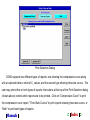
The GEOSYSTEM Swell/Consolidation Test module (CONS) is designed to reduce
laboratory data from a one-dimensional consolidation or swell test. Spreadsheet style screens
simplify the data entry process, while extensive graphics options make checking and correcting
entered data a snap.
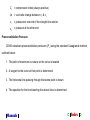
CONS specifically supports the ASTM D 2435 and D 4536 (Methods “A” and
“B”) standards.
CONS features full reduction of time-consolidation data, including both square root and log
of time methods. Coefficient of consolidation, void ratios, compression and recompression
indices, preconsolidation and swell pressures, and swell/collapse percentages are calculated
and reported by the program. For those values which are ordinarily determined using various
tangent line construction rules, the program uses similar interactive graphics constructions.
CONS has the ability to automatically perform unit conversions on all dimensions, stresses and
unit weights.
Manuals
➲ Index ➲
CONS utilizes the GEOSYSTEM Data Manager program (GDM) for all of its file processing
operations. The user should be familiar with the material in the GDM reference manual prior to
starting with this manual.
Manuals
➲ Index ➲
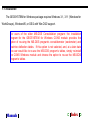
1.1 Installation
The GEOSYSTEM for Windows package requires Windows 3.1, 3.11 (Windows for
WorkGroups), Windows95, or OS/2 with Win-OS/2 support.
For users of the older MS-DOS Consolidation program: the installation
program for the GEOSYSTEM for Windows CONS module provides the
option of re-using the MS-DOS program’s consolidometer (oedometer) and
machine deflection tables. If this option is not selected, and, at a later date
the user would like to re-use the MS-DOS program’s tables, simply re-install
the CONS Windows module and choose the option to re-use the MS-DOS
program’s tables.
Manuals
➲ Index ➲
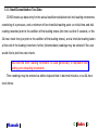
1.1.1 For Users Who Already Have GEOSYSTEM for Windows Installed
During the following installation process you will be asked which directory to install the
CONS module into. Please be sure to install it into the same hard disk subdirectory where your
GEOSYSTEM for Windows base module is already installed. (You can find the name of this
directory by selecting Help, About This Program... from the GEOSYSTEM for Windows’
opening screen and then clicking on the “System Info.” button.)
For Windows 3.1 and 3.11
Load the Windows File Manager. Place the CONS disk in a drive and click on that drive
icon. When the list of files appears, double-click on SETUP.EXE.
For Windows95
From the "Start" menu select “Run”. Place the CONS disk in a drive then select the correct
drive and type SETUP.
Manuals
➲ Index ➲
1.1.2 For Users Who Do Not Have GEOSYSTEM for Windows Installed
See Chapter 2 of the GDM manual for instructions on installing the Data Manager module.
Once the Data Manager is installed the installation program will ask you if there are more
modules to be installed. Select "Yes", place the Swell/Consolidation module disk into the same
drive the GDM disk was in, and click “Ok” to continue.
Manuals
➲ Index ➲
1.2 Hardware and Software Requirements
CONS supports the same range of hardware and software listed in Chapter 1 of the GDM
manual. CONS in particular requires 700,000 bytes of hard disk space.
CONS requires a VGA or SVGA monitor. For better viewing results, it is recommended
that the user’s Windows installation be configured for 800x600 or better resolution.
(Viewing resolution is changed using the “Display Properties” sheet in the Windows95 Control
Panel, or through the “Windows Setup” icon in the Windows 3.1/Windows for WorkGroups
“Main” program group.)
Users who have previously purchased the MS-DOS CONS program may import the older
program’s test files into the GEOSYSTEM for Windows environment. (Instructions on doing
this are given in Chapter 8.)
Manuals
➲ Index ➲
1.3 Data Requirements
CONS requires the dimensions of the consolidometer and its dial and drainage
characteristics, and optionally uses a table of deflections for mechanical loading frames. This
information is entered once during the initial setup discussed in Chapter 2 so the required
values may be retrieved from the tables using a machine or consolidometer number reference:
for each test the program will ask for the consolidometer and, optionally, the machine ID, and
retrieve the correct information from the tables.
CONS also requires Untrimmed Sample data for initial moisture, density, void ratio and
saturation calculations on the whole sample, and Trimmed or Test Specific Sample
information such as the height of the sample at the start of the consolidation test. Optionally,
the program will also utilize the Final Sample Weight.
A brief discussion of the required and optional sample and test data follows:
Manuals
➲ Index ➲
1.3.1 Untrimmed Sample Data
Untrimmed sample data is required for initial moisture, void ratio and saturation
calculations: The untrimmed sample data may be from either the actual trimmed test specimen,
or a larger sample representative of the test specimen.
Initial Moisture Weights: These are the weights for a representative sample moisture content
determination.
Sample Height and Diameter: This is the initial height and diameter of the sample as used to
calculate the soil’s unit weight; these values may be either the trimmed sample as used in the
actual consolidation test, or a larger representative sample.
Weight of Sample: This is the moist weight; as with all weights used by the program, this value
should be recorded in grams.
Manuals
➲ Index ➲
1.3.2 Test Specific Data
Specific Gravity: Entry of a specific gravity for the sample is optional; however, the program is
unable to calculate void ratios unless a specific gravity is supplied by the user.
Deflection Table Id: This is an optional data field for users with mechanical loading frames
who need to apply loading frame deflection corrections to dial readings. The program will
automatically look up the deflections for a given loading pressure. Refer to Chapter 2 for more
information about this option.
Consolidometer Number: This is a number from 1 to 20 that corresponds to an entry in the
program’s consolidometer database. The consolidometer number is required. Refer to
Chapter 2 for more information about the consolidometer data table.
Trimmed Height: Corresponds to the height of the specimen at the beginning of the
consolidation test. This entry defaults to the consolidometer height as stored in the
consolidometer table.
Manuals
➲ Index ➲
Overburden Pressure: This is an optional item that can be used by the program when
calculating the Cr, the recompression index.
Manuals
➲ Index ➲
1.3.3 Swell/Consolidation Test Data
CONS breaks up data entry for the actual swell/consolidation test into loading increments,
consisting of a pressure, and a minimum of two time/dial reading pairs: an initial time and dial
reading recorded prior to the addition of the loading stress (the time is either 0 seconds, or the
24-hour clock time just prior to the addition of the loading stress), and a time/dial reading taken
at the end of the loading increment; further (intermediate) readings may be entered if the user
would like to plot time-rate charts.
Note that the term “loading increment” is used generically to represent both
loading and unloading increments.
Time readings may be entered as either elapsed time in decimal minutes, or as 24-hour
clock times.
Manuals
➲ Index ➲
1.3.4 Post-Test Specimen Data
The post-test wet and dry sample weights may also be entered: these numbers may be
utilized for double-checking the program’s calculated dry sample weight. (If the calculated dry
sample weight, which is derived from the density and volume of the untrimmed sample,
appears incorrect, the user may force the program utilize the post-test dry weight in place of the
derived weight).
Manuals
➲ Index ➲
1.4 Data Acquisition Support
The ability to import data recorded by data acquisition equipment is an optional feature in
CONS - versions of the program customized for data import may be obtained directly from the
makers of consolidation test hardware.
Manuals
➲ Index ➲
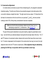
2. Configuring CONS
CONS includes a number of user-configured parameters: when the software is first
installed, the user should begin by setting up the program with the options that most closely
match the test to be run. The following sections detail the various configuration options
available.
Manuals
➲ Index ➲
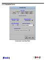
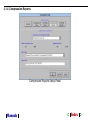
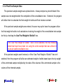
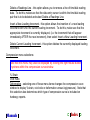
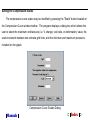
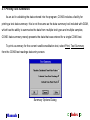
2.1 Setup Dialog
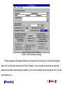
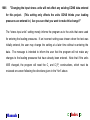
CONS program options are configured from the program's setup dialog (below). The
dialog may be accessed from two places: the first is the Options, CONS Setup menu selection
available within the GEOSYSTEM for Windows program, the second, Setup, is available from
the CONS data entry screen.
Manuals
➲ Index ➲
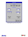
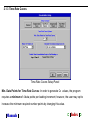
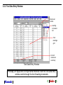
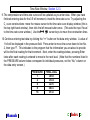
Setup Dialog Showing the General Setup Panel
Manuals
➲ Index ➲
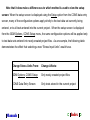
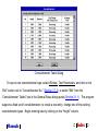
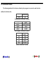
Note that it does make a difference as to which method is used to view the setup
screen: When the setup screen is displayed using the Setup option from the CONS data entry
screen, many of the configuration options apply strictly to the test data set currently being
entered, or to all tests entered into the current project. When the setup screen is displayed
from the GDM Options, CONS Setup menu, the same configuration options will be applied only
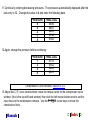
to test data sets entered into newly-created project files. As an example, the following table
demonstrates the effect that selecting a new “Stress Input Units” would have.
Change Stress Units From:
Change Affects:
GDM Options, CONS Setup
Only newly-created project files
CONS Data Entry Screen
Only tests stored in the current project
Manuals
➲ Index ➲
When creating a new project file that will be used to store data that utilize
dimension or stress units that are different than normal, make sure to change
the units (using the Options, Setup General Options... and Options, Cons
Setup menu items available from the GDM opening screen) before creating
the new project file.
The setup dialog is composed of a number of different setup panels which are viewed by
clicking on one of the five buttons grouped under Setup Category. Each panel is described in
a following section.
Manuals
➲ Index ➲
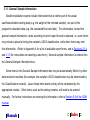
2.1.1 General Setup
Changing any of the following options while entering data for a consolidation
test defines the corresponding option for every consolidation test entered into
the current project.
Stress Units (Input): these are the units in which the loading pressures for the
Swell/Consolidation test were recorded.
If a project file was mistakenly created with the wrong stress units, open a
CONS test stored in the project, then select Setup from the CONS data entry
screen and change the “Stress Units (Input)” to the appropriate selection.
Stress Units (Output): these are the units to be used when reporting or graphing loading
pressures. Note that the output stress units may be different than the input stress units: the
program will automatically perform any necessary conversions.
Dimension Units (Output): Selects the units to be used when reporting or graphing
dimensions. Again, the output dimension units may be different from the input dimension units.
(Refer to Section 3.2 of the GDM manual for information on changing the input dimension
units.)
Manuals
➲ Index ➲
Unit Weight Units (Output): Selects the units to be used when reporting the initial wet and dry
sample densities.
Deflection Tables: Clicking this button allows the user to enter and modify loading frame
deflection tables. These tables are discussed in detail in Section 2.2.
Consolidometer Tables: Clicking this button allows the user to enter and modify
consolidometer tables. These tables are discussed in detail in Section 2.3.
Manuals
➲ Index ➲
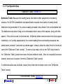
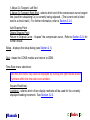
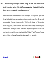
2.1.2 Compression Curves
Compression Curve Setup Panel
Manuals
➲ Index ➲
Compression Curve Starts At: The user has the option of starting the compression curve at
either the first loading stress or at the left edge of the graph. (When starting at the left edge of
the graph, the program plots from a void ratio=to the initial void ratio, a % change of 0, and a
deformation of 0.)
Compression Curve Plots: The compression curve may be plotted as the void
ratio/deformation/% change at either the final dial reading taken at each loading increment, or
at the calculated end of primary consolidation (D100) for each loading increment.
If the D100 option is chosen, loading increments without time-rate readings
will be plotted at the final dial reading for the loading increment minus the
difference between the final dial reading and D100 at the first previous loading
increment where time-rate readings were taken.
Changing this option while entering data for a consolidation test defines the corresponding
option for every consolidation test entered into the current project.
ASTM D 4546 Compatibility: If this option is chosen, hardcopy compression curve charts will
include a right-hand scale indicating % heave. (Refer to the Technical Documentation chapter
for a discussion of how % heave is calculated.)
Manuals
➲ Index ➲
Swell Pressure Calculated As: CONS will calculate swell pressure as either the pressure
required to restore the wetted sample to the void ratio at the time of wetting or the difference
between the restoration pressure and the pressure on the sample when it was wetted.
Recompression Index Is: some references define Cr as the average slope of the rebound
cycle(s), while other references define the value as the average slope of both the rebound and
recompression cycles. The program may be configured to calculate Cr by either method, or to
not or report Cr.
For swell tests, the software will always calculate Cs, the swell index, as the
average slope of the only the rebound cycle(s), and Cs will be reported in
place of Cr.
Manuals
➲ Index ➲
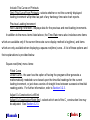
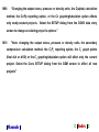
2.1.3 Time-Rate Curves
Time-Rate Curves Setup Panel
Min. Data Points for Time-Rate Curves: In order to generate Cv values, the program
requires a minimum of 4 data points per loading increment; however, the user may opt to
increase the minimum required number points by changing this value.
Manuals
➲ Index ➲
Report Cv Values As: The program supports a number of different units for reporting Cv
values. Note that the selections available depends upon the Output Units chosen from the
General Setup Options panel.
Calculate Secondary Compression As: Standard references list the secondary compression
equation as either the slope of the secondary compression line divided by the sample height, or
as divided by the height of solids. The program supports both methods; in addition, if the user
does not require secondary compression values, selecting do not calculate secondary
compression eliminates the secondary compression value from the program’s hardcopy
reports.
Changing the “Cv units” or “Secondary Compression Calculation Method”
while entering data for a consolidation test defines the corresponding option
for every consolidation test entered into the current project.
Manuals
➲ Index ➲
Default Time-Consolidation Graph is Dial Reading vs.: When a new loading increment is
entered the program displays either a square-root(time) or log(time) time-rate graph - the
setting of this option determines which graph is chosen. (Note that once a loading increment
has been entered, the user may override the default graph selection.)
Manuals
➲ Index ➲
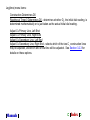
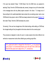
2.1.4 Compression Reports
Compression Reports Setup Panel
Manuals
➲ Index ➲
Compression Curve Report Shows: Underneath the standard consolidation graph on
hardcopy reports, the user may opt to add either a table or a graph of Cv values. Note that
neither the Cv table nor the Cv graph will be plotted unless time-rate data have been
entered for several loading increments (meaning 4 or more time/dial reading pairs per
increment).
Show Construction Lines: Optionally, CONS may be configured to show the Cc/Pc
(compression index/preconsolidation pressure) construction lines on hardcopy compression
curve reports.
Engineering Units: The user may opt to have the program display the %change/ void
ratio/deformation consolidation graph axis in divisions that are directly readable using one of
the ranges on an engineering scale. Note that the program determines whether the 10, 20, 30,
40, 50 or 60 scale is chosen.
Report Form: The program features a number of unique formats for presenting the
consolidation curve in hardcopy form. Examples of each of the report formats listed in the
Report Form box may be found in Appendix A.
Manuals
➲ Index ➲
Report Title: Each hardcopy consolidation report form includes a common title that may be
modified by the user.
Manuals
➲ Index ➲
2.1.5 Time-Rate Reports
Time-Rate Reports Setup Panel
Manuals
➲ Index ➲
Show Full Secondary Consolidation: The primary consolidation portion of many squareroot(time) curves occupies only the left 10 or 20% of the time-rate graph, making an accurate
evaluation of the Cv construction difficult. To avoid this, the user may choose to have the
program drop the linear secondary consolidation portion of the curve and expand the rest of the
curve accordingly. Note that this option is only available when plotting time-rate curves on
hardcopy reports: the on-screen square-root(time) plot instead features a zoom option.
Increment Figure Numbers: This option allows the user to specify increasing figure numbers
on successive pages of time-rate curve reports: if this option is chosen, then the figure number
printed on the consolidation curve report matches the number specified under "Figure No.:" in
the Test Parameters window (see Section 3.1); the figure number used on the first time-rate
curve report is the “Figure No.:” value increased by one; each subsequent page increments this
number by one. (Refer to page 28 of the GDM manual for a discussion of how the figure
number is incremented.)
If the user chooses not to have the program increment the figure number, the consolidation
curve report and all time-rate curve reports will show the same figure number.
Manuals
➲ Index ➲
Show Construction Lines: Optionally, CONS may be configured to show the Cv construction
lines on hardcopy time-rate curve reports.
Report Form: The program features several unique formats for presenting the time-rate curves
in hardcopy form. Examples of each of the report formats listed in the Report Form box may
be found in Appendix A.
Report Title: Each hardcopy time-rate report form includes a common title that may be
modified by the user.
Manuals
➲ Index ➲
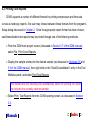
2.2 Deflection Tables
Because the loading frame can deform when subjected to increasing stresses, the ASTM
D 2435 specification requires that a table of loading frame deflections be generated for the
various loading pressures to be utilized in the consolidation test: The deflections are taken
using a non-deformable disk in place of the sample, along with (optionally) filter papers if they
will be used in the actual test. Deflection tables are stored in a database by the program so
that they may be shared between tests that use the same loading frame and loading sequence.
To view or edit the program’s database of deflection tables, select “Edit” from the
"Deflection Tables" box in the General Setup dialog panel (Section 2.1.1), or from the
“Deflection Table” prompt on the Test Parameters dialog (Section 3.1.2).
Manuals
➲ Index ➲
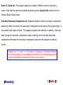
Deflection Table Dialog
Current deflection tables are shown in the Deflection Tables panel. The New button at
the bottom of the panel causes the program to create a new deflection table, and the Remove
button deletes the currently highlighted deflection table.
To view or edit an existing deflection table, click on the table ID in the Deflection Tables
panel.
Manuals
➲ Index ➲
Deflection Table Prompts:
ID: Each deflection table must be associated with a unique ID or description so that the user
may select the table from a list of deflection tables stored in the system. Enter anything into
this field, as long as it is unique from the other ID's shown in the Deflection Tables panel.
When entering pressures into the deflection table, use the stress units that will
be used to enter loading pressures for tests that will utilize the new deflection
table.
Pressure: Enter each loading pressure used in the calibration procedure in order of
application. Note that if an unload and/or reload cycle was included as part of the calibration,
the table will feature multiple entries for the same loading pressure (one for the initial loading,
one for the unload, one for the reload, etc.). This is acceptable: When the table is applied to a
consolidation test, the program will determine which of the calibration entries will be used for a
given loading increment based upon whether or not the increment was in an initial loading
cycle, an unloading cycle, or a reloading cycle.
Manuals
➲ Index ➲
Note that the loading increment immediately prior to a water-added cycle and
the actual water-added cycle share the same loading pressure and deflection:
enter a pressure/deflection line for the loading increment immediately prior to
the water-added cycle; do not enter a line for the actual water-added cycle.
Deflection: Enter the reading on the dial gauge after the given pressure was applied. Note
that the dial gauge must be zeroed prior to starting the calibration procedure. Use the
same measurement units (cms. or inches) that will be used during the actual consolidation tests
utilizing the new deflection table.
NOTE: all deflection readings should be positive.
If the dial gauge
DECREASES with compression, enter the deflection as the (positive) amount
of deflection.
Manuals
➲ Index ➲
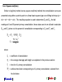
2.3 Consolidometer Tables
Several properties are common to all tests run with a given consolidometer rig, including
the diameter and height of the consolidometer, the drainage path and the direction of change
for the dial gauge. These properties are stored in the consolidometer table, from which the
user must select an entry for each new swell or consolidation test performed. (Multiple
consolidometers featuring the same diameter, height, drainage paths and dial change
directions may be incorporated into a single entry in the table).
Manuals
➲ Index ➲
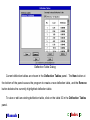
Consolidometer Table Dialog
To input a new consolidometer type, select Window, Test Parameters, and click on the
“Edit” button next to “Consolidometer No.” (Section 3.1.2), or select “Edit” from the
“Consolidometer Tables” box in the General Setup dialog panel (Section 2.1.1). The program
supports a fixed set of consolidometers: to create a new entry, change one of the existing
consolidometer types. Begin entering data by clicking on the “Height” column.
Manuals
➲ Index ➲
Consolidometer Table Columns:
Height, Diameter: Enter the height and inside diameter of the consolidometer ring. (The height
is used only to provide a default value for the Sample Height prompt in the Test Parameters
dialog.)
Note that the measurement units used for the sample height and diameter
must be identical to the measurement units to be utilized in consolidation tests
that will use the consolidometer: e.g. if measurements for the consolidation
tests will be taken in inches, enter the consolidometer height and diameter in
inches. If the same consolidometer will be utilized for tests measured in
inches AND for tests measured in centimeters, two separate consolidometer
types must be created: enter one type using centimeter dimensions and the
second using inches, then select the appropriate consolidometer on a test-bytest basis.
If the consolidation test is to be performed directly within a ring-lined sampler without trimming,
enter 0 as the consolidometer diameter: The program will assume that the diameter of the
sample during the consolidation test is identical to the value entered as the Untrimmed
Sample Diameter in the Test Parameters dialog.
Manuals
➲ Index ➲
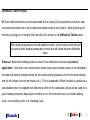
Dial Change With Compression: The program supports dial gauges that read increasing
values as the sample is compressed and gauges that read decreasing values as the sample is
compressed. Select the correct option from the list. If an incorrect selection is made, the
compression vs. log(pressure) curve for tests utilizing the consolidometer will appear
upside-down.
Drainage Path: If a porous stone was utilized on both faces of the test sample select Double;
otherwise, select Single.
Manuals
➲ Index ➲
3. Test Data Entry and Modification
To begin entering data for a swell or consolidation test, start by following the steps outlined
in Section 3.8 or Section 3.9 of the GDM manual for creating and revising a sample. When the
appropriate sample window is displayed, double-click on "Swell/Consolidation" in the Test
Modules panel. (To edit the CONS data already entered for a given sample, follow the steps
outlined in Section 3.9 of the GDM manual to re-edit the sample then click on
“Swell/Consolidation”.)
Manuals
➲ Index ➲
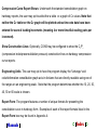
3.1 Test Parameters
If swell/consolidation data for the selected sample have not yet been entered, CONS will
begin the data entry process by displaying the Test Parameters dialog shown below. (When
revising data, the same dialog may be viewed by selecting Window, Test Parameters from the
Test Readings screen discussed in Section 3.2.)
Manuals
➲ Index ➲
CONS Test Parameters Dialog
Three categories of sample test data are entered into the dialog: the Untrimmed Sample
data, the Test Specific data and the Post-Test data. Also included are prompts for entering
general information concerning the sample, such as the sample's liquid and plastic limit, the soil
classification, etc.
Manuals
➲ Index ➲
3.1.1 General Sample Information
Swell/consolidation reports include information that is neither part of the actual
swell/consolidation testing data (e.g. the weight of the trimmed sample), nor part of the
program's calculated data (e.g. the calculated final void ratio). This information, termed the
general sample information, varies according to which report format is selected; i.e. some forms
may include a place for listing the sample's USCS classification, while other forms may omit
this information. (Refer to Appendix A for a list of available report forms, and to Sections 2.1.4
and 2.1.5 for instructions on selecting a new form.) General sample information is entered into
the General Sample Information box.
Some items in the General Sample Information box may be automatically filled in by other
data reduction modules (for example, the sample's USCS classification may be determined by
the Classifications module). Leave these items blank as they will be completed by the
appropriate module. Other items, such as the testing remarks, will need to be entered
manually. For further instructions on entering this information, refer to Section 3.6 of the GDM
manual.
Manuals
➲ Index ➲
3.1.2 Test Specific Data
Deflection Tables, Section 2.2.
Deflection Table: Because the loading frame can deform when subjected to increasing
stresses, the ASTM Consolidation test specification requires that a table of loading frame
deflections be generated for the various loading stresses to be utilized in the consolidation test:
The deflections are taken using a non-deformable disk in place of the sample, along with filter
papers, if they will be used in the actual test. Deflection tables remain entered into the program
indefinitely, so if a table appropriate to the current loading frame and loading sequence has
already been entered, it need not be entered again; instead, select the table from the list shown
next to the “Deflection Table” prompt. To enter a new table, click on the “Edit” button next to
the “Deflection Table” prompt then enter the new deflection table. After the new table has been
entered, make sure to select it from the “Deflection Table” prompt.
If a deflection table was not taken, select (none) from the list shown next to the “Deflection
Table” prompt.
Consolidometer Tables, Section 2.3.
Manuals
➲ Index ➲
Consolidometer No.: Several properties are common to all tests run with a given
consolidometer rig, including the diameter and height of the consolidometer, the drainage path,
and the direction of change for the dial.
For a new consolidometer, click on the “Edit” button next to the “Consolidometer No.” prompt
then enter the consolidometer parameters. Because these tables are permanently stored by
the program, after a table has been entered, for subsequent tests the user may simply enter the
appropriate table number at the “Consolidometer No.” prompt.
Sample Height at Test Start: Enter the trimmed height of the sample at the start of the test.
The trimmed diameter of the sample is assumed to be equal to the diameter
of the consolidometer ring as entered into the consolidometer table selected
for use with the test.
Overburden Pressure: This is an optional parameter used to indicate the pressure exerted by
the overburden material on the sample: If entered, the pressure is used by the program in
recompression index calculations (as discussed in the Technical Documentation chapter).
Leave the prompt blank if the pressure was not recorded.
Manuals
➲ Index ➲
Time Values Entered As: For the entry of loading increments where time-rate data are desired
the program will accept time readings as either the decimal number of minutes elapsed since
the start of the current loading increment (e.g. 1.5 min), or the current clock time in 24-hour
format (e.g. 01:23:24). This selection must be made before data for any loading increments
have been entered - changing the selection after time-rate readings have already been entered
will cause existing readings to be erased.
If time-rate data (D100 and Cv values) are not desired and the user intends to
enter just initial and final time/dial readings for each loading increment, the
"Elapsed Time" option should be selected.
Manuals
➲ Index ➲
3.1.3 Initial (Untrimmed) Sample Data
Enter all weights in grams.
Wet Weight+Tare, Dry Weight+Tare, and Tare Weight: These values are used to determine
an initial (natural) moisture percentage for the sample. Note that the weights are not the
weights of the sample to be used in the consolidation test; rather, they are from additional
material sampled from the same location as the consolidation test sample. If more than one
moisture content test was performed, select the data from the test most representative of the
consolidation sample.
Untrimmed Sample Height, Weight and Diameter: These values may actually be either from
the untrimmed sample, or from the trimmed sample, as long as all three are from the same
source (trimmed or untrimmed). The weight, height and diameter values are used to calculate
the initial (natural) density.
Specific Gravity: This parameter is optional; however, if it is left blank, the program will not
calculate void ratios.
Manuals
➲ Index ➲
3.1.4 Post-Test Sample Data
The post-test sample weights are optional items - these prompts may be left blank if the
sample was not weighted after the completion of the consolidation test. If entered, the program
will utilize them to calculate the final weight of solids and final moisture content.
If the post-test sample weights are entered, the user may opt to have the program utilize
the final weight of solids in all calculations involving the weight of the consolidation test sample:
do this by checking the Use Final Weight of Solids? box.
If the “Use Final Weight of Solids?” box is to be selected, the final moisture
content test must have been run using the entire sample that was utilized in
the actual swell/consolidation test.
If the post-test weights aren't entered, or if the “Use Final Weight of Solids?” box isn't
selected, then the program will utilize an estimated weight of solids based upon the dry weight
of the untrimmed sample multiplied by the ratio of the volume of the untrimmed sample to the
volume of the trimmed sample.
Manuals
➲ Index ➲
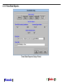
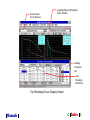
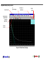
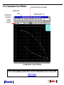
3.2 Readings Data Entry/Curve Display Screen
The readings data entry/curve display screen consists of the compression curve window,
the log(time)/root(time) curve window, and the test readings data entry window. These
windows allow the user to enter data and view graphed results all on the same screen.
Manuals
➲ Index ➲
Compression
Curve Window
Log(time)/Square Root(time)
Curve Window
Loading
Increment
List
Test
Readings
Data Entry
Test Readings/Curve Display Screen
Manuals
➲ Index ➲
Note that only one window at a time may receive input from the keyboard: this window is
called the “focus” window, and has a title bar shown in blue and white (using the default
Windows coloring scheme). Switch focus from one window to another by clicking the left
mouse button once while the mouse pointer is in the title bar of the window you want to
activate, or select the appropriate window from the Window menu.
Each of the windows on the test readings screen can be maximized to the full size of the
screen by clicking on the
(or
in Windows95) button shown in the top right-hand corner of
the window. Reduce the window to its original size by clicking on the lower
(or
in
Windows95 button.
Manuals
➲ Index ➲
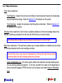
3.2.1 Menu Selections
Print menu selections:
Test Reports - begins the process of printing or previewing test reports by displaying
the print selection dialog. Refer to Section 4.2 for details on this option.
Test Summary - begins the process of printing test summaries. Refer to Section 4.1
for details on this option.
Window menu selections: lists the four available windows on the test readings data entry
screen. Selecting a window from the list will shift the focus to that window.
The window that currently has the focus is listed next to a check mark.
Edit menu selections: The edit menu allows you to make additions or deletions to be made
to the data entered into the test readings window.
Note that this menu may also be displayed by clicking the right mouse button
anywhere within the test readings data entry window.
Insert a Readings Line - this menu option allows the insertion time/dial reading data
into an existing loading increment. To do this, position the cursor at the beginning of
the line that will appear AFTER the line to be inserted, and select Insert a Readings
Line.
Manuals
➲ Index ➲
Delete a Readings Line - this option allows you to remove a line of time/dial reading
data. To do this, make sure that the data entry cursor is within the time/dial reading
pair that is to be deleted and select Delete a Readings Line.
Insert a New Loading Increment - this option allows the insertion of a new loading
increment BEFORE the current loading increment. To do this, make sure that the
appropriate increment is currently displayed, (i.e. the increment that will appear
immediately AFTER the new increment), then select Insert a New Loading Increment.
Delete Current Loading Increment - this option deletes the currently displayed loading
increment.
Compression menu selections:
Note that this menu may also be displayed by clicking the right mouse button
anywhere within the compression curve window.
% Strain
Void Ratio
Deformation - selecting one of these menu items changes the compression curve
window to display %strain, void ratio or deformation versus log(pressure). Note that
this selection also determines which type of compression curve is included on
hardcopy reports.
Manuals
➲ Index ➲
1 Adjust Cc Tangent, Left End
2 Adjust Cc Tangent, Right End - selects which end of the compression curve tangent
line (used for calculating Cc) is currently being adjusted. (The current end is listed
next to a check mark.) For further information, refer to Section 3.2.4.
Add Shaping Point
Delete Shaping Point
Return to Original Curve - “shapes” the compression curve. Refer to Section 3.2.4 for
further details.
Setup - displays the setup dialog (see Section 2.1).
Quit - closes the CONS module and returns to GDM.
Time-Rate menu selections:
Note that this menu may also be displayed by clicking the right mouse button
anywhere within the time-rate curve window.
Square-Root(time) Log(time) - selects which of two display methods will be used for the currently
displayed loading increment. See Section 3.2.3.
Manuals
➲ Index ➲
Include This Curve on Printouts
Omit This Curve From Printouts - selects whether or not the currently displayed
loading increment will printed as part of any hardcopy time-rate chart reports.
Previous Loading Increment
Next Loading Increment - displays data for the previous and next loading increments.
In addition to the menu items listed above, the Time-Rate menu also includes some items
which are available only if the current time-rate curve display method is log(time), and items
which are only available when displaying a square-root(time) curve. A list of these options and
their explanations is provided below.
Square-root(time) menu items:
Fitted Curve
Linear Curve - the user has the option of having the program either generate a
mathematically modeled curve based upon the time/dial readings for the current
loading increment, or just draw a series of straight lines between successive time/dial
reading points. For further information, refer to Section 3.2.3.
Adjust Cv Construction Left End
Adjust Cv Construction Right End - selects which end of the Cv construction line may
be adjusted. See Section 3.2.3.
Manuals
➲ Index ➲
Log(time) menu items:
Construction Determines D0
Reading at Time=0 Determines D0 - determines whether D0, the initial dial reading, is
determined mathematically or is just taken as the actual initial dial reading.
Adjust Cv Primary Line, Left End
Adjust Cv Primary Line, Right End
Adjust Cv Secondary Line, Left End
Adjust Cv Secondary Line, Right End - selects which of the two Cv construction lines
may be adjusted, and which end of that line will be adjusted. See Section 3.2.3 for
details on these options.
Manuals
➲ Index ➲
3.2.2 Test Data Entry Window
Next load
button
Loading
increment
list
Test
readings
grid
Current
increment
summary
Test Data Entry Window
Pressing Ctrl-PgUp and Ctrl-PgDn while the focus is on the Test Data Entry
window scrolls through the list of loading increments.
Manuals
➲ Index ➲
Swell/Consolidation tests are composed of loading increments, which consist of loading
pressures along with at least two time/dial reading pairs - an initial time at 0 minutes and the
dial reading prior to the application of the loading pressure, and the elapsed time (in decimal
minutes or clock time) at the end of the test along with the dial reading at the end of the test.
Intermediate time and dial readings may be entered for some or all loading increments if the
user would like to obtain C values for these increments.
v
The term “loading increment” is used generically to indicate both loading and
unloading increments.
Begin entering data for a loading increment by specifying the loading pressure in response
to the "Pressure:" prompt. Make sure that the correct stress units are displayed next to the
prompt - if they aren't, choose the Setup menu option, then select the appropriate units from the
General Setup panel (Section 2.1.1).
Manuals
➲ Index ➲
Saturation cycles are entered by typing a "w" or "s" in response to the "Pressure:" prompt,
then pressing ENTER. This indicates to the program that the loading pressure has not
changed, but that the current increment consists of readings taken following the addition of
water to the sample.
Manuals
➲ Index ➲
Each test may be set up to accept either 24-hour clock times or elapsed times: the choice
is made from the Test Parameters dialog discussed in Section 3.1. The column headings on
the test readings grid indicate which option was chosen for the current test:
Elapsed Time indicates that the program expects times to be entered as the decimal number
of minutes (e.g. 1 min. 30 seconds should be entered as "1.5") elapsed from the application of
the current loading pressure. Elapsed times may be entered with a precision of .01 minutes.
24 Hr. Clock indicates that times are to be entered as 24 hour clock readings rounded to the
nearest second (e.g. 1:00 PM should be entered as "13:00:00"). After the initial clock reading
for each loading increment, the user must also enter the number of days elapsed since the
application of the current loading pressure. These times are entered as "+DD HH:MM:SS" "DD" is the number of complete days elapsed since the application of the current loading
pressure, "HH:MM:SS" is the current clock time, again, in 24-hour format. Note that the
program will automatically enter the "+", " " and ":" symbols: "+01 13:23:12" should be typed as
"01132312".
Manuals
➲ Index ➲
Note that the program does not recognize daylight-savings time changes.
The user must manually add or subtract an hour from clock times taken after
the time change ONLY during the loading increment being processed during
the time change. Clock times for subsequent loading increments may be
entered as-is.
Dial readings may be entered with a precision of up to .00001 inches or centimeters. The
program includes an automatic dial divisor option designed to save a few keystrokes per
reading: with the selection of the appropriate divisor, the user can enter "2631" instead of
"0.2631". Once each reading is entered, the program divides the number entered by the divisor
to obtain the true dial reading. Select an appropriate divisor from the "Dial Divisor" selection
box shown in the data entry window's toolbar. If "1" is selected as the dial divisor, the program
will expect that actual dial readings will be entered.
The first time/dial reading pair entered in the test readings grid should be at time=0: the
dial reading should be identical to the final dial reading taken on the previous loading
increment; for the first loading increment, enter the initial reading on the dial prior to the
application of any pressure.
Manuals
➲ Index ➲
For tests without time-consolidation data, enter F in the second line of the table for the
elapsed time (the program will display "final" for the time), then enter the final dial reading.
(After doing this once, CONS will assume that subsequent loading increments will only include
the final dial reading, automatically display "final", and jump directly to the readings column.)
Note that this option is valid only when entering elapsed times (as opposed to 24-hour
clock readings).
After the final dial reading has been entered for the loading increment, pressing Enter twice
will begin a new loading increment.
When entering time-rate data for Cv calculations, the user should check the
time-rate curve display window to make sure that the Cv constructions for the
current loading increment have been properly placed prior to starting a new
loading increment.
To create a saturation cycle, enter all of the time/dial reading pairs taken for the loading
increment prior to the addition of water, then start a new loading increment. Enter a “W” or “S”
as the loading pressure for the new increment, then enter the time/dial readings taken between
the time the water was added and the application of the next loading pressure.
Manuals
➲ Index ➲
The Loading Increment List
On the right-hand side of the test data entry window the program maintains a list of the
loading increments entered into the current test file. A symbol is shown to the left of each
increment in the list; the symbol indicates the following:
This indicates that the corresponding time-rate curve will be included on hardcopy reports
that include time-rate curves.
This indicates that the corresponding time-rate curve will NOT be included on hardcopy
reports. There are three possible reasons for this condition:
1. The user manually selected the “DO NOT PRINT” time-rate toolbar button.
Manuals
➲ Index ➲
2. The program was unable to calculate a Cv value for the corresponding loading
increment. If the Cv value shown in the time-rate curve display’s status window reads
“n/a”, then the program could not calculate a valid Cv value--this is usually due to a
problem with the adjustment of the Cv construction lines.
3. The time-rate curve has not been viewed on the screen. If a change is made to the data
in the test’s parameters window, or if the loading increment was acquired from an
external data file (this is an optional feature), then the time-rate curve for the loading
increment must be viewed on the screen prior to printing. (To view the curve, follow the
instructions below.)
To view the data and time-rate curve for a loading increment, click the left mouse button
with the mouse cursor located on the appropriate increment in the loading increment list.
Manuals
➲ Index ➲
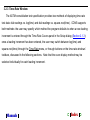
3.2.3 Time-Rate Window
The ASTM consolidation test specification provides two methods of displaying time-rate
test data: dial readings vs. log(time) and dial readings vs. square-root(time). CONS supports
both methods: the user may specify which method the program defaults to when a new loading
increment is entered through the Time-Rate Curves panel in the Setup dialog (Section 2.1.3);
once a loading increment has been entered, the user may switch between log(time) and
square-root(time) through the Time-Rate menu, or through buttons on the time-rate windows’
toolbars, discussed in the following sections. Note that the curve display method may be
selected individually for each loading increment.
Manuals
➲ Index ➲
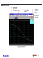
Log(Time) Curve
Construction
adjustment
endpoint selection
D0 calculation
method
Include on
printouts
button
Curve type
selection
Log(time) Window
Manuals
➲ Index ➲
The log(time) window displays a graph of dial reading vs. log10(elapsed time). The purpose
of this window is to allow the user to adjust the construction lines used to determine D0, D100 and
Cv for the current loading increment.
Note that the Cv value is presented in the units selected from the time-rate
curves panel of the setup dialog. All other calculated values and scales are
displayed in the units selected to represent entered data.
Manuals
➲ Index ➲
Cv Construction Adjustment
The log(time) method requires the placement of a line tangent to the steepest portion of
the time-rate curve (called the primary construction line), and a second line tangent to the final
readings which represent a straight-line trend (called the secondary construction line). The
intersection of these two lines represents D100.
Make sure that the time-rate display window has the “focus” prior to
attempting to adjust the Cv constructions. (See Section 3.2.)
These two lines may be moved one end at a time by using the up and down cursor keys.
Use the End key to alternate between moving the left and right ends of each line. The four
buttons labeled "PL", "PR", "SL" and "SR" window's toolbar indicate which end of which line is
currently being adjusted: when the "PL" button is depressed, the left endpoint of the primary
construction line may be moved, "PR" depressed means that the right end of the primary
construction line will be moved, etc. A finer adjustment may be obtained by pressing the
Shift key in conjunction with the up and down cursor keys.
Manuals
➲ Index ➲
The intersections between the construction lines and the curve are shown in
red as an aid to properly placing the tangents.
To determine D0 the program requires an additional construction consisting of two vertical
lines labeled "t0" and "4t0". These lines represent a time ratio of 1 to 4 on the curve: D0 is taken
as the dial reading at time "t" minus the difference between the dial readings at "4t" and "t".
Adjust the location of the interval using the left and right cursor keys - note that the program will
not allow the interval to end at a time corresponding to less than 1/4 of the total deformation for
the loading increment or at a time corresponding to greater than 1/2 of the total deformation.
Again, a finer adjustment may be obtained by pressing the Shift key in conjunction with
the left and right cursor keys.
The time interval construction will only appear if the selection box shown in
the window's toolbar indicates that D0 is "construction".
Manuals
➲ Index ➲
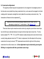
Toolbar Objects
•
These buttons select which end of the Cv construction lines may currently be
adjusted. (Refer to the previous section.)
• The selection box labeled "D0 is" determines whether D0 is determined using the
interval construction discussed above, or taken to be the actual dial reading at the
time the current loading pressure was applied. If the D0 value determined from the
interval construction differs significantly from the actual dial reading at time t=0,
change the selection box to read "initial dial" - the program will use the actual dial
reading at time t=0 as D0
•
The printer button indicates whether or not the current time-rate curve and
calculated Cv value will be included on hardcopy time-rate printouts. If the icon is
shown with a red "X", the curve will not be included as part of the hardcopy time-rate
reports.
Manuals
➲ Index ➲
•
Click on this button to change the time-rate method for the current loading
increment to be dial reading vs. square-root(time).
•
This button merely indicates that the current time-rate display method is dial reading
vs. log(time).
Manuals
➲ Index ➲
Square-Root(Time) Curve
Zoom factor
Cv
percentage
Include on
printouts
Curve
type
Construction
adjustment
endpoint
selection.
Curve
model
Square-Root(time) Display
Manuals
➲ Index ➲
The square-root(time) window displays a graph of dial reading vs. square-root(elapsed
time). The purpose of this window is to allow the user to adjust the construction lines used to
determine D0, D90 and Cv.
Note that the Cv value is presented in the units selected from the time-rate
curves panel of the setup dialog. All other calculated values and scales are
displayed in the units selected for the inputted data.
Manuals
➲ Index ➲
Cv Construction Adjustment
Cv constructions are shown as a pair of lines intersecting at D0, the program's calculated
initial dial reading. The left-most of the two lines should be tangent to the initial points of the
curve which indicate a straight line trend. The right-most line has a slope 1.15 times that of the
left-most; the intersection of this line with the curve provides T90 and D90, the time and dial
reading at which 90% of the primary consolidation has been completed.
Make sure that the time-rate display window has the “focus” prior to
attempting to adjust the Cv constructions. (See Section 3.2.)
The pair of lines used to determine D0 may be moved by using the up and down cursor
keys. Use the End key to alternate between moving the left and right ends of the lines. The "L"
and "R" buttons in the window's toolbar indicate which ends of the lines will be moved: when
the "L" button is depressed, the left endpoint of the construction lines may be moved; the right
endpoints move when the "R" button is depressed. A finer adjustment may be obtained by
pressing the Shift key in conjunction with the up and down cursor keys.
Manuals
➲ Index ➲
The intersection between the Cv construction line and the curve is shown in
red as an aid to properly placing the tangent.
The T90 intersection is indicated by a vertical line which may be moved left or right by
pressing the left or right cursor keys. Again, a finer adjustment may be obtained by pressing
the Shift key in conjunction with the left and right cursor keys.
Manuals
➲ Index ➲
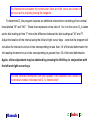
Toolbar Objects
•
These buttons select which end of the Cv construction lines may currently be
adjusted. (Refer to the previous section.)
Note that the selection of the curve drawing method has no effect on the
calculated D0 value, and little overall effect on the calculated D 90 and Cv
values. The choice been the linear and fitted methods is mainly made for
aesthetic reasons.
Manuals
➲ Index ➲
• The selection box listing "Fitted" and "Linear" determines whether the curve is drawn
by using a smoothed, mathematically generated shape (i.e. "Fitted"), or as a series of
straight lines drawn between readings ("Linear"). Each curve drawing option has its
own advantages and drawbacks: The “Fitted” method mathematically smoothes out
any time-rate readings that may not lie on an idealized curve form. For example, if the
sample quit consolidating temporarily due to friction between the sample and the ring,
a couple of data points on the time-rate curve may not accurately follow the actual
consolidation curve for the soil. The fitted curve will minimize the effect of problems
such as this.
However, because the fitted curve is an artificial model for a physical process, there
are curves for which an accurate model cannot be generated. Also, the curve fitting
process is much slower than the process of drawing point-to-point (linear) curves:
because the “Linear” method simply draws straight lines between adjacent time/dial
reading pairs, the time-rate window displays faster. The drawback to the linear method
Manuals
➲ Index ➲
is that because it incorporates no data smoothing, outlying data points will have a
much larger effect over a given section of the curve.
• The "Zoom" scrollbar allows the user to zoom in on the left-hand portion of the curve
as an aid in properly placing the Cv constructions. Note that this does not affect any
hardcopy views of the curve.
• The selection box listing percentages allows the user to calculate a Cv value at a
different percentage of primary consolidation than the default value of 90%.
•
The printer button indicates whether or not the current time-rate curve and
calculated Cv value will be included on hardcopy printouts. If the icon is shown with a
red "X", the curve will not be included as part of the hardcopy time-rate reports.
•
Click on this button to change the time-rate method for the current loading
increment to be dial reading vs. log(time).
•
This button merely indicates that the current time-rate display method is squareroot(time).
Manuals
➲ Index ➲
3.2.4 Compression Curve Window
Construction
adjustment
endpoint
selection
Compresison
Units
Click to select the curve scales
Swell Pressure
Compression Curve Window
If the curve appears upside-down, see the compression curve FAQs in the
Help! chapter.
Manuals
➲ Index ➲
The compression curve window displays a graph of % change, void ratio, or deformation
vs. log (pressure). From this window, the user has the option to adjust the construction lines
10
used to determine the preconsolidation pressure (Pc) and compression index (Cc) values, to
choose the type of compression graph (%change, void ratio or deformation) and to specify the
scales to be used on the graph.
Note that the pressure and deformation scales are shown in the "Output
Stress" and "Output Dimension" units selected from the General Setup dialog
(Section 2.1).
Manuals
➲ Index ➲
Cc and Pc Construction Adjustment
Make sure that the time-rate display window has the “focus” prior to
attempting to adjust the compression curve constructions. (See Section 3.2.)
The compression index (Cc) line, shown in cyan, should be tangent to the steep, linear
portion of the compression curve. The endpoints of the line may be adjusted individually by
using the up and down cursor keys; use the End key to alternate between moving the left and
right ends of the line. The "L" and "R" buttons in the window's toolbar indicate which end of the
line will be moved: when the "L" button is depressed, the left endpoint of the construction line
may be moved; the right endpoint moves when the "R" button is depressed. Note that a finer
adjustment may be obtained by pressing the Shift key in conjunction with the up and
down cursor keys.
As an aid in placing the tangent line, the intersection between the line and the
compression curve turns red.
Manuals
➲ Index ➲
The preconsolidation pressure (Pc) calculation requires the location of the point of
maximum curvature on the consolidation curve - this point is automatically chosen by the
program and marked with a red vertical line. This location may be adjusted by using the left
and right arrow keys; again, note that a finer adjustment may be obtained by pressing the Shift
key.
Manuals
➲ Index ➲
Curve Shaping
Circular markers are plotted on the curve to indicate the calculated
compression points; “shaping” points are indicated by crosses.
Once data have been entered, the program will display the compression curve which may
be shaped by adding or deleting “shaping” points. These additional points are treated the same
as actual test points by the program’s calculation routines. Insert shaping points where there is
not enough natural data to provide the shape required of the curve. The following sections
discuss the available curve shaping options:
Note that the shaping menu discussed in the following sections may be
accessed by clicking the right mouse button anywhere within the curve display
screen.
Manuals
➲ Index ➲
To add a point:
Once started, all shaping procedures may be aborted by selecting the
Compression, Return to Original Curve menu option.
The shape of the compression curve may be modified by forcing it to pass through a new
point. To do this, select the Compression, Add Shaping Point menu item. The program will
respond by highlighting a section of the curve: prior to adding the actual shaping point, the user
must select the curve section to which the point will be added (the program breaks the curve up
into compression, rebound and recompression sections). Move the mouse until the desired
curve segment changes from white to red, then click the left mouse button to select the
segment. Next, position the mouse pointer at the desired location for the new shaping point
and click the left mouse button again. The new shaping point will be marked with a "+" and the
curve will be immediately modified to accommodate the new point.
Manuals
➲ Index ➲
To delete a shaping point:
To remove a shaping point, select the Compression, Delete Shaping Point menu option.
If the curve contains one shaping point, the point will be immediately removed. If more
than a single shaping point has been added to the curve, the shaping point nearest the mouse
pointer will be shown with a box around it. Move the cursor until the desired shaping point is
highlighted then click the left mouse button. A message will appear noting that the shaping
point has been removed.
Manuals
➲ Index ➲
Removing all shaping points
Selecting Compression, Return to Original Curve removes all shaping points.
Manuals
➲ Index ➲
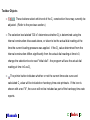
Toolbar Objects
•
These buttons determine which end of the Cc construction line is currently
adjustable. (Refer to the previous section on Cc and Pc adjustment for further
information.)
• The selection box labeled "Type" allows the selection of one of three units for the
deformation scale: % change (in void ratio/sample height), void ratio, or deformation.
All are plotted against log(pressure). Note that this selection does not affect C , P or
c
C.
r
Note that the void ratio vs. log(pressure) graph may not be selected if the
user did not enter a specific gravity for the current sample (See Section
1.3.2.)
• The "Scale" button allows the user to specify the scales to be used on the
compression graph. For further information, refer to the next section.
Manuals
➲ Index ➲
c
Setting the Compression Scales
The compression curve scales may be modified by pressing the "Scale" button located on
the Compression Curve window toolbar. The program displays a dialog box which allows the
user to select the maximum ordinate axis (i.e. % change, void ratio, or deformation) value, the
scale increment between two ordinate grid lines, and the minimum and maximum pressures
included on the graph.
Compression Curve Scales Dialog
Manuals
➲ Index ➲
When entering values, make sure to select values appropriate to the selected output stress
and dimensional units: Keep in mind that these units may be different than the units used to
enter the pressure and dial readings: if so, the changed scale values will not be reflected in the
on-screen compression curve display. (See General Setup Options, Section 2.1.1, for further
information.)
The scale selections may be reset to program-determined default values by either deleting
the contents of each data entry field in the scale dialog and setting the minimum pressure scale
to "(default)", or by clicking on the "Reset" button.
On % strain scales, if the maximum value is a percent compression (as
opposed to a percent swell), enter the value as a negative number.
Manuals
➲ Index ➲
3.3 Editing Data For An Existing Swell/Consolidation Test
To edit swell/consolidation data already entered for a given sample, follow the steps
outlined in Section 3.9 of the GDM manual to re-edit the sample, then click on
“Swell/Consolidation” in the Test Modules panel.
Manuals
➲ Index ➲
4. Printing Test Summaries and Reports
CONS generates both graphical chart reports and text summaries of the data entered for a
single test.
Manuals
➲ Index ➲
4.1 Printing Test Summaries
As an aid in validating the data entered into the program, CONS includes a facility for
printing a test data summary: this is not the same as the data summary tool included with GDM,
which has the ability to summarize the data from multiple test types and multiple samples;
CONS’ data summary merely presents the data that was entered for a single CONS test.
To print a summary for the current swell/consolidation test, select Print, Test Summary
from the CONS test readings data entry screen.
Summary Options Dialog
Manuals
➲ Index ➲
Prior to printing the summary the program displays the Summary Options dialog shown
above - after selecting the appropriate options, select “Ok” to continue. From this dialog, the
following options may be selected:
Tabulate Calculated Time-Rate Values: If this option is selected, then the program will
include the Cv and Cα values as part of the "End-of-Load" summary table.
Tabulate Time-Rate Readings: If this option is selected, the program will print a table of
elapsed time and dial reading for each loading increment where intermediate elapsed time/dial
reading data were taken.
Include Time-Rate Charts: Selecting this option causes a miniature chart of dial reading vs.
time to be included alongside the elapsed time/dial reading table for each loading increment.
Note that this option may only be selected after the "Tabulate Time-Rate Readings" option has
been selected.
Manuals
➲ Index ➲
4.2 Printing Test Reports
CONS supports a number of different formats for printing compression and time-rate
curves as hardcopy reports - the user may choose between these formats from the program’s
Setup dialog discussed in Chapter 2. Once the appropriate report format has been chosen,
swell/consolidation test reports may be printed through one of the following methods:
• From the GDM main project screen (discussed in Section 3.7 of the GDM manual),
select File, Print Cons Reports.
• Display the sample window for the desired sample (as discussed in Sections 3.8 and
3.9 of the GDM manual), then right-click on the "Swell/Consolidation" entry in the Test
Modules panel, and select Print Test Reports.
This method and the following one automatically select for printing the report
that includes the currently selected sample.
• Select Print, Test Reports from the CONS opening screen, as discussed in Section
3.2.
Manuals
➲ Index ➲
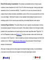
Print Selection Dialog
CONS supports two different types of reports: one showing the compression curve along
with an optional table or chart of Cv values, and the second type showing time-rate curves. The
user may print either or both types of reports: the buttons at the top of the Print Selection dialog
(shown above) control which reports are to be printed. Click on "Compression Curve" to print
the compression curve report, "Time-Rate Curves" to print reports showing time-rate curves, or
"Both" to print both types of reports.
Manuals
➲ Index ➲
The "Existing Sources and Swell/Consolidation Tests" lists the sources and CONS tests
entered into the current project file. Sample sources are listed next to folder icons: click on a
source name to list the swell/consolidation tests associated with the source.
Tests are listed next to CONS icons: click on a test to select that test for printing. Once a
test has been selected for printing, the CONS icon listed next to that test is changed into a
printer icon: clicking on a test shown next to a printer icon changes the test’s status back to “not
selected for printing”. (Note that, if "Print", "Test Reports" was selected from the CONS data
entry screen, the test currently being edited will automatically be selected for printing.)
Clicking on the "Select All" button marks all tests in the currently open source for printing;
likewise, the "Deselect All" button unselects all tests in the currently open source.
Begin the actual report printing process by clicking on the "Print" button, which prints the
reports on the currently selected printer, or by clicking on the "Preview" button, which displays
the reports on-screen.
Examples of the report formats supported by the program are presented in
Appendix A.
Manuals
➲ Index ➲
5. Technical Specifications
The following chapter details the calculations employed by CONS to produce the results
listed on the program's output. Units are omitted from the following sections for simplification.
Manuals
➲ Index ➲
5.1 Calculation of Specimen Parameters
Moisture, density, initial void ratio and saturation values are calculated from the
measurements on the sample. There are some variations among laboratories in the
procedures followed when recording these measurements. Briefly, the different procedures
handled by the program and what effect they have on calculations are as follows:
1. The dimensions and weight of a larger sample, not the actual test specimen, are
recorded. The height of the actual test specimen is also recorded and entered in the
program. In this case, the weight of the test specimen is found by multiplying the weight
of the larger sample by the ratio of test specimen volume to the volume of the larger
sample.
Data for procedures 1 and 2 are entered into the “Initial (Untrimmed)” panel in
the Test Parameters dialog (Section 3.1.3).
Manuals
➲ Index ➲
2. The actual test specimen dimensions and weight are recorded and entered in the
program. This is the simplest case, and the program calculates the moisture, density,
saturation, etc. directly from the measurements. The weight of solids is determined
from the test specimen’s wet weight and moisture content.
This information is entered into the Test Parameters “Post-Test” panel.
3. As an alternative to using the weight of solids calculated by CONS from the initial
specimen, the user may enter a dried post-test specimen weight.
The following sections detail the calculation procedures utilized by the software. Note that
the equations assume that dimensions are given in centimeters and weights are in grams.
(Unit conversion factors are listed in Section 5.5).
Manuals
➲ Index ➲
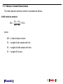
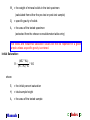
5.1.1 Moisture Content Determination
The initial (natural) moisture content is calculated as follows:
Initial moisture content:
MCi =
W wt − W dt
* 100%
W dt − Wt
where:
MC = initial moisture content
i
W
wt
= weight of wet sample with tare
W
dt
= weight of dried sample with tare
W
t
= weight of the tare
Manuals
➲ Index ➲
5.1.2 Wet and Dry Density Determination
The initial (natural) wet and dry densities are calculated from the untrimmed specimen as
follows:
Wet density:
γwi =
Wt
Vt
where:
γwi
= initial wet density
Wt = specimen weight
Vt
= volume
and:
π* (Dt) 2 * Ht
Vt =
4.0
where:
Manuals
➲ Index ➲
Vt
= volume
Dt
= diameter
Ht
= total height
Dry density:
γ =
di
γwi
2 H
D
*
(1 + MCi / 100) D * H
c
c
t
t
where:
γdi
= total sample dry density
Dc
= the diameter of the consolidometer
Hc
= the height of the sample in the consolidometer
Manuals
➲ Index ➲
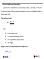
5.1.3 Void Ratio and Saturation Determination
The initial void ratio and saturation are calculated from the actual test specimen size and
weight as follows:
Initial void ratio:
eo =
(Ht − Hs)
Hs
where:
eo
= initial void ratio
Ht
= specimen test height
Hs
= height of solids
and:
Hs =
W d / Gs
At
where:
Manuals
➲ Index ➲
Wd = the weight of mineral solids in the test specimen
(calculated from either the pre-test or post-test sample)
Gs = specific gravity of solids
At
= the area of the tested specimen
(extracted from the chosen consolidometer table entry)
Void ratios and initial/final saturation values will not be reported for a given
sample unless a specific gravity is entered.
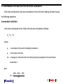
Initial Saturation:
Si =
(MCi * W d)
* 100
(Ht − Hs) * At
where:
Si
= the initial percent saturation
Ht
= total sample height
At
= the area of the tested sample
Manuals
➲ Index ➲
5.1.4 Post-Test Specimen Calculations
A post-test moisture-content test is not mandatory; however, if performed, and the entire
test specimen is used for the moisture content sample, the user may opt to use the resulting
final dry weight as Wd.
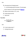
Final moisture content:
MCf =
W wt − W dt
W dt − W t
where:
MCf = final moisture content
Wwt = final weight of wet sample with tare
Wdt = final weight of dried sample with tare
Wt = tare weight
Weight of solids (calculated from post-test sample data):
Wd = Wdt - Wt
Manuals
➲ Index ➲
where:
Wd = weight of solids calculated from the post-test sample
Manuals
➲ Index ➲
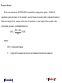
5.2 Intermediate Void Ratio and Percent Strain Calculations
Void ratios and percent strain are calculated at the end of each loading increment using
the following equations:
Intermediate Void Ratio
Void ratios subsequent to the initial void ratio are calculated as follows:
en = eo - δe
where:
en
= void ratio at the end of loading increment n
eo
= the initial void ratio
δe = change in void ratio from the initial (pre-test) sample to the end of load
increment n
and:
(DRn − DRc) − DRo
δe =
Hs
Manuals
➲ Index ➲
where:
DRn = dial reading at the end of the loading increment:
D100, or the final dial reading entered for the increment. (The choice depends
upon the “Compression Curve Plots” option discussed in Section 2.1.2)
DRc = deflection correction (optional), or 0 if D100 is used
DRo = initial dial reading at start of test
Hs
= height of solids
Percent Strain:
%Sn =
(DRn − DRc) − DRo
* 100%
Ho
where:
%Sn = % strain for loading increment “n”
Ho = initial height of test specimen
Manuals
➲ Index ➲
Percent Heave:
If the user selects the ASTM D 4546 compatibility configuration option,. CONS will
calculate a percent heave for the sample - percent heave is percent strain, adjusted relative to
either the height of the sample at the time of inundation, or the height of the sample at the
overburden pressure (modified Method A):
%HVn =
DRn − DRi
* 100%
Hi
where:
%HVn= the percent heave
Hi
= height of the sample at the time of inundation/overburden pressure
Manuals
➲ Index ➲
5.3 Consolidation vs. Log(Pressure) Curve Calculations
Void ratio, percent strain or deformation is plotted against the log(applied pressure) using a
cubic spline curve fitting method. Once data points are fit to a curve, Pc (preconsolidation
pressure), Cc (compression index), Cr (recompression index) and (if applicable) swell pressure,
percent heave/swell and Cs (swell index) values are determined using the equations outlined
below:
Compression Index
The compression index (Cc) is defined as the slope of the straight-line portion of the
consolidation curve. It is expressed as a ratio of the change in void ratio to the change in log of
pressure over the straight-line portion of the compression curve:
Cc =
δe
log(σ 2 / σ1)
where:
Manuals
➲ Index ➲
Cc
= compression index (always positive)
δe = void ratio change between σ1 & σ2
σ1
= pressure at one end of the straight-line section
σ2
= pressure at the other end
Preconsolidation Pressure
CONS calculates preconsolidation pressures (Pc) using the standard Casagrande method,
outlined below:
1. The point of maximum curvature on the curve is located
2. A tangent to the curve at that point is determined
3. The horizontal line passing through that same point is drawn
4. The equation for the line bisecting the above lines is determined
Manuals
➲ Index ➲
5. The point is located where the tangent to the linear portion of the virgin
consolidation curve meets this bisector line (the same tangent is used that
was selected for the Cc): Pc is equal to the pressure corresponding to this point.
Recompression/Swell Indices
CONS will calculate and report a value for either Cr, the recompression index, or Cs, the
swell index, depending upon whether or not a saturation cycle was included as part of the test:
for tests that include a saturation cycle, Cs is calculated; otherwise, the program calculates Cr.
Cs is always the average of the slopes of the unloading cycles. Depending upon the user’s
selection for the “Recompression Index is” option in the “Compression Curves” setup dialog
panel, Cr will be either the average slope of the reload portions of the curve, or the average of
the unload and reload slopes.
If an overburden pressure is entered and the preconsolidation pressure is greater than the
overburden pressure then the slope averaging will only be performed on the portion of the
curve between the overburden and preconsolidation pressure.
Manuals
➲ Index ➲
Saturation Cycles
CONS includes the capability to accept data from saturation cycles and report the
corresponding swell percentage and pressure, defined and calculated as follows:
Swell percentage: The difference between the percent swell/consolidation before and after
sample wetting.
Swell pressure: Depending upon the setting of the “Swell Pressure Calculated As” option in the
“Compression Curves” setup dialog panel, the swell pressure is calculated as either the
additional pressure needed to restore the sample to the percent consolidation attained prior to
wetting, or as simply the pressure needed to restore the sample to the percent consolidation
attained prior to wetting.
Manuals
➲ Index ➲
5.4 Time-Consolidation Calculations
Time-consolidation procedures are dependent upon which test method is selected;
log(time) or square root(time). The following sections detail the calculations involved with each
method.
Manuals
➲ Index ➲
5.4.1 Log(time)
Log(time) method time-consolidation curves are presented using a least-squares type
curve fitting technique (a+bx+cx2+dx3+ex4). The resulting curve equation is used to find D0 and
D100, the dial readings at 0 and 100 percent primary consolidation, as discussed in Chapter 3.
D50 and T50, the dial reading and time at 50 percent primary consolidation, may then be
calculated, and the result used to determine Cv:
0.197 * Hp 2
Cv =
T 50
where:
Cv
= coefficient of consolidation
0.197
= time factor corresponding to 50% consolidation
T50
= time for 50% primary consolidation
Hp
= the average drainage path length during the current loading increment
and:
Manuals
➲ Index ➲
Hp =
(Ho − δHt − (δHn / 2))
DF
where:
Ho = initial height of the specimen
δHt = the total deformation of the specimen up to loading increment n
δHn = the change in specimen height during load n:
this is either D100-D0 or the final dial reading for loading increment n - the last
dial reading of increment (n-1), depending upon the “Compression Curve Plots”
setting of the compression curve panel on the setup dialog
DF = the drainage path factor = 1 for single drainage and 2 for double drainage
Manuals
➲ Index ➲
Cα, the coefficient of secondary compression, is calculated as the slope of the right-hand
Cv construction line divided by either the height of solids (Hs) or the initial sample height (H0):
this choice is based upon the “Calculate Secondary Compression As” setting of the Time Rate
Curves setup dialog panel (see Section 2.1.3).
X (%)
10
20
30
40
50
60
70
80
90
Manuals
TIME
.008
.031
.071
.126
.197
.287
.403
.567
.848
➲ Index ➲
5.4.2 Square-root(time)
Similar to log(time) method curves, square-root(time) method time consolidation curves are
presented using either a point-to-point or a linear least-squares type curve fitting technique (a +
b/x + c/x2 + d/x3 + e/x4). The resulting equation is used to determine D0 and D90, the dial
readings at 0 and 90 percent primary consolidation; these values are in turn utilized to calculate
D100 and Dx (where x is the percent of consolidation corresponding to Cv) and Tx and Cv.
D100 = D0 - 10/9(D0 - D90)
TFx * Hp
Cv =
Tx
2
where:
Cv
= coefficient of consolidation
Hp = the average drainage path length, as explained in the previous section
Tx
= time for x% primary consolidation
TFx = unitless time factor corresponding to x% primary consolidation, selected from
the list below:
Manuals
➲ Index ➲
5.5 Conversion Factors
The following tables list the factors utilized by the program to convert to and from the
software’s internal units.
*
centimeters
inches
2.54
Dimensional Conversion Factors
g/cm3
÷
lbs./ft.3
(30.483)/453.59
kg/m3
1000
3
kN/m
9.8067
Unit Weight Conversion Factors
÷
kg/cm2
tsf
1.024
ksf
2.048
psf
2048.2
kPa
98.0687
Stress Conversion Factors
Manuals
➲ Index ➲
5.6 Data Exported by the Program
For each entered test, CONS calculates a number of different data items that may be used
on data summaries created by the GDM "Data Summary and Export" tool. Additionally, these
items, or "variables", may be referenced in boring logs and data summaries created with the
GEOSYSTEM LOGDRAFT program (version 3.3 or later). The following table lists the name of
all the calculated variables provided by CONS, and provides a short description of each
variable. Note that all data are stored in the output dimension, stress and density units that
were in effect the last time the test file was edited by CONS.
Item Name
SPECGR
Description
This is the specific gravity as entered by the user into the Test
Parameters dialog.
E0
INIT_SAT
Initial saturation.
CSNMI
Natural moisture.
CS_DENS
OVER
Manuals
Initial void ratio - blank if a specific gravity is not specified.
Natural density.
Overburden pressure.
➲ Index ➲
Item Name
OCR
Description
“OverConsolidation Ratio”: this is the ratio of the overburden
pressure to the preconsolidation pressure. This value is blank if
the user does not enter an overburden pressure.
DIDCONS
“Y” for every sample for which a swell or consolidation test was
entered. Use the GDM Data List/Export tool to provide a count of
the number of swell/consolidation tests performed on a project.
DIDSWELL
“Y” for samples where a consolidation test was performed AND the
sample was wetted.
PP
Preconsolidation pressure.
CC
Compression index.
CS
Swell index - only stored for wetted samples.
RECOTYPE
SWELL_PRESS
“Cs “ for un-wetted samples, “Cr ” for wetted samples.
Restoration pressure for a wetted sample - calculated using the
method specified from the program’s “Setup” dialog.
SWELL
Percent swell - calculated using the method specified from the
program’s “Setup” dialog.
CVALL
Contains a list of all calculated coefficients of consolidation and
related loading pressures.
EF
Final void ratio.
FINAL_SAT
Final saturation.
CSMF
Manuals
Final moisture content
➲ Index ➲
6. Tutorial
1. Before starting this tutorial, proceed through the tutorial presented in Chapter 6 of the
GDM manual. If the GDM tutorial was just completed, the sample window for Sample 3, from
Boring B-4 will currently be displayed by GDM.
If the appropriate sample window isn’t currently displayed, do the following:
a) Start the software by double-clicking on the “GEOSYSTEM for Windows” icon in the
“GEOSYSTEM” program group.
b) From the opening screen, select File, Open Project. When the project dialog box is
displayed, select the project called “DEMO” - it will be located in the same directory as the
GEOSYSTEM for Windows software.
c) From the main project screen, click on “Boring B-4”, then double-click on "S-3”.
CONS setup dialog, Section 2.1.
2. Select Options, CONS Setup, then select Compression Report from the Setup Categories
box. Select CSCONS3 as the Report form. Click on the Ok button to continue.
3. From the sample data dialog, double-click on the Swell/Consolidation icon in the Test
Modules box.
Manuals
➲ Index ➲
CONS Test Parameters Screen, Section 3.1.
4. The next screen to appear is the CONS Test Parameters screen. Enter the following general
sample info. in the box at the top of the Test Parameters screen:
Liquid Limit: 32
Plasticity Index: 14
USCS: CL
AASHTO:
Figure No.: 2B
Testing Remarks: Tested by ALV
5. Proceed to the box titled “Test Specific Data”. Enter the following data:
Consolidometer No. 20
Sample Height at Test Start (in.) 1.00
You may leave Deflection Table at “(none)” and Overburden Pressure blank.
Also leave “Time Values Entered As” at “elapsed time”.
6. Enter the following data into the “Initial (Untrimmed) Sample Data” box:
Initial (Untrimmed Sample Data)
Post-Test Sample Data
Wet Weight + Tare: 41.54
Height: 0.80
Wet Weight + Tare:
Dry Weight + Tare: 33.28
Diameter: 2.50
Dry Weight + Tare:
Tare Weight: 17.63
Weight: 109.20
Tare Weight:
Specific Gravity: 2.70
Leave the Post Test Sample Data box blank.
Manuals
➲ Index ➲
7. Select Close to continue. The Test Readings Data Entry Screen will now appear. Choose
“1000” as the dial divisor, then enter 0.25 as the pressure. Next, enter the following data:
Test Readings Screen, Section 3.2.
1
2
3
4
5
6
7
8
9
10
11
12
13
14
15
Manuals
Elapsed
0
.10
.25
.5
1
2
4
8
15
30
60
120
240
480
1407
Dial
2700
2697
2695
2690
2688
2682
2672
2668
2666
2664
2660
2652
2648
2642
2638
➲ Index ➲
8. Once the data above have been entered, press Enter twice (or click on the ">>" button) to
move to the next load increment. CONS will automatically select a loading pressure of 0.5
for the new increment: press Enter to accept this value, then enter the following data:
No.
1
2
3
4
5
6
7
8
9
10
11
12
13
14
15
16
Manuals
Elapsed
0
.10
.25
.5
1
2
4
8
15
30
60
120
240
480
1300
1435
Dial
2638
2505
2485
2467
2438
2397
2360
2318
2305
2298
2292
2282
2274
2264
2257
2253
➲ Index ➲
Time-Rate Window, Section 3.2.3.
9. The compression and time-rate curves will be updated as you enter data. When you have
finished entering data for the 0.5 tsf increment, check the time-rate curve. Try adjusting the
Cv curve constructions: move the mouse cursor to the time-rate curve display window (this is
the top right-hand window), then click the left mouse button once. (This sets the input “focus”
to the time-rate curve window.) Use the
cursor keys to move the construction lines.
çèéê
10.Continue entering test data by clicking the “>>“ button on the data entry window. A value of
1 tsf will be displayed in the pressure field. Press enter to move the cursor down to line No.
2, then type "f". This indicates to the program that the information you are about to provide
will be the final reading for that increment. Next, enter the readings below, pressing Enter
twice after each reading is entered to move to the next load. (Note that the numbers listed in
the PRESSURE column below correspond to individual pressures, not the “No.” column on
the data entry screen.)
PRESSURE
1
2
4
8
16
Manuals
FINAL DIAL
1868
1544
1205
0841
0532
➲ Index ➲
11.Continue by entering decreasing pressures. The pressures automatically displayed after the
last entry is 32. Change this value to 8 and enter the following data:
PRESSURE
8
4
2
1
.5
FINAL DIAL
0538
0597
0663
0732
0782
12.Again, change the pressure before continuing:
PRESSURE
1
2
4
8
FINAL DIAL
0772
0752
0686
0587
Compression Curve Window, Section 3.2.4.
13.Adjust the Cc/Pc curve constructions: move the mouse cursor to the compression curve
window (this is the top left-hand window) then click the left mouse button once to set the
input focus to the compression window. Use the
cursor keys to move the
construction lines.
çèéê
Manuals
➲ Index ➲
Printing Test Summaries, Section 4.1.
14.Print a test summary by selecting Print, Test Summary from the menu. The Summary
Options dialog will appear: select all three options then click on the “Ok” button to continue.
CONS will produce a two page summary similar to the one shown in Section 4.1.
Printing Test Reports, Section 4.2.
15.Next, print a test report for the sample: begin by selecting Print, Test Reports from the
menu. The Print Selection dialog will appear: begin by clicking on the "Both" button so that
reports for both the compression and time-rate curves will be produced.
16.When the “Preview” button is clicked, the entire report as it will be printed by the printer
appears on screen, reduced so that it can be seen in its entirety. Select Continue from the
menu to display the time-rate report, then select Continue to return to the Print Selection
dialog.
17.To reports, select the “Print” button. A printer option box will appear. When all of the
options are correct, select the Ok button to continue with the printout. The printed reports
should look like those shown in Appendix . Select Close to close the window, Quit to exit
CONS (all data will be saved), then File, Save and Exit to leave GEOSYSTEM for Windows.
Manuals
➲ Index ➲
7. Help!
CONS includes on-line, context-sensitive assistance for users with questions. To active it,
simply click on the Help menu item or command button. If you don’t find an answer to your
question in the program’s help, be sure to check the frequently asked questions section in this
chapter. If you’re still stuck, please feel free to contact GEOSYSTEM Software directly. We do
not charge for technical support, but we do ask that you be at your computer when you call,
with your data easily accessible. Also, please know the operating system and computer model
you are using as well as your printer type and network brand (if applicable).
If you have a question regarding the program’s calculations, print out and fax to us a test
summary that includes tabulated time-rate readings. Instructions for producing the test
summary may be found in Section 4.1.
You may contact us at:
Phone 970-223-8788
Fax: 970-223-0668
Email: [email protected]
Manuals
➲ Index ➲
7.1 Frequently Asked Questions
General
Q. CONS produced an error message and terminated. What should I do?
A. Under normal circumstances, the program should never shut itself down. If, for some
unusual reason CONS cannot continue, the program will produce a message indicating what
went wrong, and then terminate itself. If this happens, make a note of the message and call
GEOSYSTEM Software.
Q. How do I copy CONS data files from one machine to another?
Q. Can I use DOS to delete CONS data files?
A. Refer to the Frequently Asked Questions chapter in the GDM manual.
Manuals
➲ Index ➲
Data Entry
Q. Why does the program immediately change the dial reading values that I enter?
A. CONS multiplies all dial readings by the number listed in the “Dial Divisor” box. Make sure
to take this number into account when entering dial readings, or change the divisor to “1” if
you wish to enter true dial readings. Note that CONS does not incorporate a way to
automatically correct dial readings that were entered while an incorrect divisor was
selected: these readings must be re-entered after the correct divisor has been selected.
Q. How do I change the initial test parameters such as the sample height, weight, etc.
A. Select the “Window” menu option, then choose “4. Test Parameters”.
Manuals
➲ Index ➲
Time-Rate Curves
Q. Why does the dial reading axis for the time-rate curve appear incorrect?
A. There are three possible reasons why the dial reading axis for the points plotted on the
time-rate curves does not appear to match the actual entered data: if the test utilized a
deflection table, a deflection is being subtracted from each reading before it is plotted.
Secondly, the dial readings may have been entered using an incorrect dial divisor - refer to
the first question in the “Data Entry” section. Thirdly, the program is capable of plotting dial
readings entered in inches onto a centimeter scale, and vice versa. Check the setting of the
“Dimensional Units (Output)” box on the General Setup panel (see Section 2.1.1). If this
setting is correct, refer to the question regarding incorrect dimension units listed in the
Frequently Asked Questions chapter of the GDM manual.
Q. Why does the program show the complete square-root(time) curve for some loading
increments, even if the “Show Full Secondary Consolidation” setup option was set to “No”?
A. On some curves the secondary consolidation interval begins so close to the end of the
loading increment that chopping off the secondary consolidation interval would not gain
much display space for the primary consolidation portion of the curve; for these loading
increments, CONS displays the entire curve.
Manuals
➲ Index ➲
Q. Why doesn’t my time-rate curve print on hardcopy reports?
A. There are three possible reasons why the time-rate curve is not included in hardcopy
reports:
1) The user manually selected the “DO NOT PRINT” time-rate toolbar button.
2) The program was unable to calculate a C value for the corresponding loading
increment. If the C value shown in the time-rate curve display’s status window reads
“n/a”, then the program could not calculate a valid C value--this is usually due to a
problem with the adjustment of the C construction lines.
v
v
v
v
3) The time-rate curve has not been viewed on the screen. If a change is made to the
data in the test’s parameters window, or if the loading increment was acquired from
an external data file (this is an optional feature), then the time-rate curve for the
loading increment must be viewed on the screen prior to printing. (To view the data
and time-rate curve for a loading increment, click the left mouse button with the
mouse cursor located on the appropriate increment in the loading increment list.)
Q. Why does the C value in the time-rate curve status window show “n/a”?
v
A. An incorrect adjustment of the curve’s C construction lines can result in a situation where
the software cannot calculate a meaningful C value. Additionally, selecting the “DO NOT
PRINT” time-rate toolbar button disables reporting of a C value.
v
v
v
Manuals
➲ Index ➲
Compression Curves
Q. My compression curve appears upside-down. What’s going on?
A. Two general types of dial gauges are available: those that give increasing readings as the
consolidation sample is compressed, and those that give decreasing readings. CONS is
designed to work with both types: as part of the test parameters for the sample, a
consolidometer table entry is chosen - the setting of the “Dial Change with Compression”
option for the chosen entry tells the program what type of gauge was used for the test.
If the compression curve appears upside-down, then the “Dial Change with Compression”
setting is reversed: select Window, Test Parameters, then note the number listed next to the
“Consolidometer No.” prompt. Next, click on the “Edit” button shown next to the prompt. Go
to the consolidometer table row corresponding to the number noted above, then switch the
setting of the “Dial Change with Compression” entry for that row: if the setting is currently
“Increasing”, change it to “Decreasing”; if the setting is “Decreasing”, change it to
“Increasing”. Click on the “Close” button, then select Close from the menu. The
compression curve should appear in the correct orientation.
Manuals
➲ Index ➲
Q. Why does the stress scale for the compression curve appear incorrect?
A. Most likely, an incorrect selection was made for either the “Stress Units (Input)” or “Stress
Units (Output)” options. Select Setup and verify that the correct choice was made for both
options. (Note that if the “Stress Units (Input)” selection differs from the “Stress Units
(Output)” selection, then CONS will convert the loading pressures entered into the units
selected as “Stress Units (Output)”.
Q. After I’ve selected a new scale for my compression curve, why doesn’t the scale shown in
the Compression Curve on-screen window change?
A. The Scale dialog discussed in Section 3.2.4 allows the user to change the scales used to
display the compression curve. However, if the units selected for the “Stress Units (Input)”
differ from the units selected for the “Stress Units (Output)” then the selected curve scales
will only be applied when the curve is printed on a hardcopy report.
Q. Under what circumstances does the program report C instead of C ?
s
r
A. If water was added to the sample during the test, CONS will report C , which is the average
slope of the rebound cycle(s). If water was not added, C , the average of either just the
rebound cycle(s) or both the unload and reload cycles will be reported.
s
r
Manuals
➲ Index ➲
Hardcopy Printouts
Q. Will the software generate reports on A-4 paper?
A. Yes. Make sure that you have selected A-4 paper for the currently defined default printer.
CONS will automatically reformat the report from letter-size to A-4 size.
Q. Can I include my company logo on CONS reports?
A. Yes. Users who have licensed the GEOSYSTEM LOGDRAFT program typically receive a
digitized logo file with their LOGDRAFT package: CONS can utilize this file to include the
logo on all consolidation reports.
Users who have not licensed LOGDRAFT may choose to have GEOSYSTEM Software
digitize their logo for use with CONS; there is a small fee for the work involved. (If your
company logo is already in a machine-readable format, we may be able to use your copy.)
Manuals
➲ Index ➲
Q. The report formats included with CONS do not suit my needs. Can a custom report format
be designed?
A. GEOSYSTEM Software can custom-design a CONS report format to fit the specific
requirements of your organization. Although there is a fee for this service, it will typically be
much smaller than we have charged in the past, due to a change in the way we design the
forms.
If you would like to receive a quote on the costs involved in duplicating your report, mail or
fax us a copy of your format.
Q. On my HP LaserJet, text that is rotated, such as the "Dial Reading" label, is not printed
correctly. What's wrong?
A. Your Windows printer driver has a bug. In some cases GEOSYSTEM Software can supply
a replacement driver.
Manuals
➲ Index ➲
7.2 Error Messages
Major error and warning messages provided by the program are presented with an error
number - these messages are listed and discussed below. Note that the following list only
discusses messages provided by the Swell/Consolidation module.
1000
"The data file for this sample was created with a newer version of CONS. You
will need to use the newer program to read this file."
The CONS data file you are attempting to edit was created by another version of the
CONS program. Usually this means that you have two copies of the software on your
computer: use the “Help”, “About This Program...” menu option, then choose the “System
Info.” button to list the date the program was generated. Compare the dates of the two
copies and erase the older copy.
Manuals
➲ Index ➲
When the program resets the test’s Cv constructions, time-rate data and
curves associated with the sample will not be included on hardcopy reports
until each curve has been previewed on-screen. You can do this by
repeatedly clicking the “>>“ button in the test readings window until the end of
the loading increments list has been reached.
1001
"The specific gravity associated with this test has been changed.
All Cv
constructions will be reset: You must review each time-rate curve on-screen."
This indicates that the specific gravity associated with the sample was changed by another
data reduction module, or through LOGDRAFT.
This change means that CONS must
recalculate all testing information, so the Cv and Cc/Pc constructions will be reset. Note that
the time-rate curves and data associated with the sample will not be included on hardcopy
reports until each curve has been previewed on-screen.
Manuals
➲ Index ➲
1002
"The consolidometer data associated with this test have changed.
All Cv
constructions will be reset: Review each time-rate curve on-screen."
1003
"The deflection table associated with this test has been changed.
All Cv
constructions will be reset: You must review each time-rate curve on-screen."
Modifying consolidometer or deflection information invalidates the calculated test data for
any samples that use the modified consolidometer entry or deflection table. The next time
the sample is loaded, CONS will detect that the sample’s consolidometer or deflection
table has been changed, and will recalculate all testing information based upon the
modified information. All Cv and Cc/Pc constructions will be reset - make sure to review
each time-rate curve on-screen prior to printing a test report.
Manuals
➲ Index ➲
1004
"WARNING. The deflection table selected for use with this test no longer exists.
The table selection will be reset."
The deflection table used for the test was deleted or ID associated with the table was
changed. Because the deflection table could no longer be located, the program has reset
all deflections to 0, and all Cv and Cc/Pc constructions have been reset. Make sure to
review each time-rate curve on-screen prior to printing a test report.
1005
"Note: due to a sample data change, the time-rate constructions have been
reset. Review all time-rate curves on-screen."
Changing a test parameter such as the sample height causes the program to recalculate
all testing information based upon the modified parameter. This resets the Cv and Cc/Pc
constructions, which must be reviewed on-screen prior to printing a test report.
Manuals
➲ Index ➲
1006
"Changing the input stress units will not affect any existing CONS data entered
for this project.
(This setting only affects the units CONS thinks your loading
pressures are entered in.) Are you sure that you want to make this change?"
The “stress input units” setting merely informs the program as to the units that were used
for entering the loading pressures. If an incorrect setting was chosen when the test was
initially entered, the user may change the setting at a later time without re-entering the
data. The message is intended to inform the user that the program will not make any
changes to the loading pressures that have already been entered. Note that if the units
ARE changed, the program will reset the Cv and Cc/Pc constructions, which must be
reviewed on-screen following the directions given in the “hint” above.
Manuals
➲ Index ➲
1007
"Note: selecting a new report form may change the fields listed in the General
Sample Information section of the Test Parameters window. You should check this
window for new prompts prior to printing any reports."
Different report forms print different data items: for example, the compression report form
“A” may list the date the sample was taken, while compression report form “B” may omit
the sample date. If the user changes from form “B” to form “A” (through the “Compression
Report” Setup panel), a new field will be added to the General Sample Information panel
so that a sample date may be entered. When the Compression report form or Time-Rate
report form is changed, the user should select the “Window”, “Test Parameters” menu
option and check the General Sample Information panel for any new fields.
Manuals
➲ Index ➲
1008
“Changing the output stress, pressure or density units, the C(alpha) calculation
method, the Cc/Pp reporting option, or the Cv graphing/tabulation option affects
only newly-created projects. Select the SETUP dialog from the CONS data entry
screen to change an existing project's options."
1010
"Note: changing the output stress, pressure or density units, the secondary
compression calculation method, the Cc/Pp reporting option, the Cc graph points
(final dial or d100) or the Cv graphing/tabulation option will affect only the current
project. Select the Cons SETUP dialog from the GDM screen to affect all new
projects"
Manuals
➲ Index ➲
If the user has selected “Setup”, “CONS Setup” from the GDM menu (as opposed to
selecting “Setup” from the CONS test data entry screen), changes to any of the items listed
in the message above will only affect projects created in the future. To change one of
these settings for the swell/consolidation tests entered into an existing project, start a new
CONS test for the project or edit a CONS test already entered into the project (Section 3.3)
then select “Setup” from the CONS test data entry screen.
Conversely, if the user has changed one of the listed settings while editing a CONS test,
the changed setting will only be applied to the tests entered into the current project.
This procedure is designed to allow the user to create projects that utilize different test
methods or measurement units without affecting any existing project files.
If the Cc graph point option is changed from final dial to D100 (or vice versa) for
a given project, it is recommended that the user edit each of the CONS tests
entered into the project and re-adjust the Cc/ Pc constructions.
Manuals
➲ Index ➲
1012
"A water-added cycle already exists."
CONS supports a single inundation cycle: the message means that an attempt was made
to enter a duplicate loading pressure, indicating an inundation cycle. This message usually
implies a data entry error where the user may have inadvertently entered the same loading
increment twice.
1013
"The void ratio plot is not available due to an invalid initial void ratio. (Probably,
a specific gravity was not selected for the sample.)"
The program cannot calculate void ratios without a valid specific gravity. Check the Test
Parameters dialog (Section 3.1) to make sure a specific gravity has been entered.
Note that CONS does not require a specific gravity for the sample unless the user desires
void ratio values.
Manuals
➲ Index ➲
1014
"Note: changes made to a deflection table will not affect an existing
consolidation tests utilizes that table UNTIL the test is revised."
If a change is made to a deflection table, the testing information calculated for any
swell/consolidation tests already entered that utilize that table will be invalid. Because the
program does not automatically revise the calculations for these tests, the user is
responsible for revising each test file (see Section 3.3). Doing this causes the program to
recalculate any data that may have changed when the deflection table was changed.
1015
"The selected ID is not unique: this ID is used by another deflection table. Enter
a different ID."
The ID used to identify the deflection table must be unique. Select an ID that does not
match one of the table ID’s shown in the “Deflection Tables” panel.
Manuals
➲ Index ➲
1016
"You must enter an ID for the table"
CONS identifies deflection tables by ID’s, which are unique names consisting of any
combination of letters or numbers. Prior to entering deflection information for a new table,
you must enter a unique ID for the table.
1017
"Note: changes made to a consolidometer entry will not affect an existing
consolidation tests utilizes that consolidometer UNTIL the test is revised."
If a change is made to a consolidometer entry, the testing information calculated for any
swell/consolidation tests already entered that utilize that consolidometer will be invalid.
Because the program does not automatically revise the calculations for these tests, the
user is responsible for revising each test file (see Section 3.3). Doing this causes the
program to recalculate any data that may have changed when the consolidometer entry
was changed.
Manuals
➲ Index ➲
1018
"WARNING: you have chosen to switch this test from clock time to elapsed
time. Are you sure that you want to do this?"
1019
"WARNING: changing from elapsed time to clock time - all test readings will be
DELETED! ARE YOU SURE THAT YOU WANT TO PROCEED?"
Once CONS test readings have been entered for a given sample, making a change to the
“Time Values” selection (discussed in Section 3.1.2) will cause the program to erase all
existing test readings. Be absolutely sure that you actually want to make the change there is no way to recover any data lost through making the wrong selection.
1022
"Changing the input stress units affects only projects created in the future."
This message is for informational purposes only: it does not indicate an error.
The
message indicates that the input stress units were changed from GDM’s Options, Cons
Setup menu, and that the current project (if one is being edited) will not be affected by the
change.
Manuals
➲ Index ➲
To change the input stress units for an existing project, use GDM to open the project file
(refer to Section 3.12 in the GDM manual), then open a sample window (GDM manual
Sections
3.8
and
3.9),
and
open
the
CONS
program
by
clicking
on
the
“Swell/Consolidation” entry in the “Test Modules” window. Next, select Setup and choose
the correct stress units. This selection will affect every test entered into the current project
file.
Manuals
➲ Index ➲
8. Converting DOS CONS Data Files
The Swell/Consolidation module includes a tool to convert data from the MS-DOS
GEOSYSTEM CONS program into a format readable by the Windows module. To convert a
MS-DOS CONS data file into a Windows file, first open the GEOSYSTEM for Windows project
file into which the test file is to be placed, then follow the steps for entering a new sample or
revising an existing sample that are detailed in Sections 3.8 and 3.9 in the GDM manual: this is
the sample that will be associated with the MS-DOS CONS test file. Once a sample data
window for the correct sample is displayed, select Tools, DOSCONS File Conversion.
Note that for licensed copies, installation of the file conversion tool is an
option: if DOSCONS File Conversion doesn’t show up under the GDM Tools
menu, you must re-install the CONS module: during the installation, make
sure to select “Yes” when asked about installing the conversion program.
After the menu selection, the file conversion utility will request the complete path to the
MS-DOS CONS program. Make sure to enter a complete path, including the disk drive name,
e.g. “C:\GEOSYS\CONS”.
Manuals
➲ Index ➲
If, after selecting the DOSCONS File Conversion menu item, a warning is
displayed noting that a Swell/Consolidation data file already exists for the
current sample, the program has found a Windows Swell/Consolidation test
data file that has already been created for the sample. Proceeding with the
file conversion process will overwrite the existing Windows data file.
If the conversion program is able to locate a copy of the MS-DOS CONS program at the
specified path, a list of tests stored by the MS-DOS program will be displayed. Double-click on
the appropriate test to perform the conversion.
Once the file has been converted into a GEOSYSTEM for Windows format, it may be
viewed by re-opening the sample data window, then clicking on the “Swell/Consolidation” entry
in the Test Modules panel of the window. Initially, a message will be displayed indicating that
the specific gravity associated with the sample has been changed: ignore this message. The
program will proceed to display the test readings screen for the sample - make sure to open the
Test Parameters window and check the deflection table and consolidometer number for the
test, as these values may not be correct. If desired, an overburden pressure may also be
entered: since the MS-DOS program did not include the option to enter an overburden
pressure, this value will initially be blank.
Manuals
➲ Index ➲